The Journal of Science Extension Research ( b ) H RP Phy i cal Param t r ( 15) TOTPOT ME HR MA GAM F X ... t l 0 t2 ...._,, !Zl 0.. 0 .... !Zl 0 t9 8 . ..... l:--< t lO Data
Targets -----~~!! tt,t.k NSW Department of Education Volume 2, 2023
Samples
Image credit:
Cover - Vincent Ng, James Ruse Agricultural High School
Inside cover - Minalu de Graaf, Lambton High School

NSW Department of Education

Table of Contents The Journal of Science NSW Department of Education Extension Research 2023 i'1k NSW GOVERNMENT 4 Forewords 7 Acknowledgments 8 Introduction 12 In this edition 19 Student reports ···················· ···················· ····················
Foreword
Matthew Scott
Curriculum Secondary Learners
In my role as Coordinator of Science, TAS, Mathematics and STEM secondary curriculum teams, I am well positioned to see how ground breaking the Science Extension course is and the positive impact it has on the students in NSW schools which is evident in the work presented in this volume of the Journal of Science Extension Research.
The Science Extension course really is a game changer in our science classrooms. From its innovative science content such as the history and philosophy of science, data science and ethics, to being the first HSC course to be examined online and also first Stage 6 science course to incorporate a student research project as a substantial part of the course mark. Further innovation in the Science Extension course are the opportunities that students have to work on projects that transcend the syllabus.
In December 2015, the Education Council presented a case for change though its National STEM School Education Strategy 2016 - 2026, where over the next five years, employment was predicted to increase in professional, scientific and technical services by 14 per cent and in health care by almost 20 per cent. The strategy called for a renewed national focus on STEM in school education being critical to ensuring that all young Australians are equipped with the necessary STEM skills and knowledge that they will need to succeed.

Building on this, the office of Australia's Chief Scientist 2020 report 'Australia's STEM Workforce', highlighted that Australians who have studied science, technology, engineering and mathematics (STEM) are helping to solve the problems of the future.
Evidence of how young people in our schools are making their contribution to solving the problems of the present and future can be found in Volume 2 of The Journal of Science Extension Research. Health challenges like the efficacy treatments Crohn's Disease, to environmental challenges such as the impact of microplastics on seafood, technological challenges like the effectiveness of sound absorbing materials
PEO STEM Coordinator -
r :')
Journal
Science
The
of
2023 .t'1k NSW GOVERNMENT
NSW Department of Education Extension Research
Foreword continued

through to disproving misconceptions around black holes, students in NSW public schools are proving that the Science Extension course is preparing them to meet these future workforce needs for STEM professionals.
Equally important to the development of the necessary STEM skills and knowledge in students is the role of the Science Extension teachers and professional mentors. Meeting the needs of the course while preparing to work as researchers, the support they provide our students is critical to their success not only in Science Extension but in their future after school.
I commend the efforts of the student, teacher and mentor teams that have resulted in the selection of the reports in the journal, of which all are of the highest quality. It will be exciting to see the direction taken by future students of Science Extension with the support of their teachers and mentors. Will they investigate how we can meet electricity demand and generation needs, adapt to the changing climate, integrate Al safely and appropriately into society and optimising healthcare for ageing populations? Time will tell, and I look forward to seeing what the following future STEM professionals will discover.
The Journal of Science NSW Department of Education Extension Research 2023 .t'1k NSW GOVERNMENT
James demonstrates the chaotic behaviour of his circuit
Foreword
Dr Steven Goldfarb Honorary Fellow, University of Melbourne Former Chair, International Particle Physics Outreach Group
I am honoured to introduce this 2nd volume of The Journal of Science Extension Research. The NSW Science Extension syllabus is a world-leading program for secondary science education, as the quality of articles in this volume make evident. The content covers a wide range of relevant topics that clearly presented exciting challenges to the students taking part in the research.
The invention of the World-Wide Web at CERN sparked an unprecedented communication revolution around the globe. Everyone everywhere suddenly had access to everything, with instant communication at their fingertips. While the advantages were predictable, its usage by bad actors, seeking fame, financial or political gain blindsided many of us; it can pose an important risk to the mindset of young students, even when they have been raised in this environment. Nobody is immune.
This is why research opportunities, such as the Science Extension syllabus, play such an important role. By pursuing challenging scientific investigation into areas that pique their interest, these young scientists develop skills and learn valuable lessons. This pertains not only to their specific topics, but also the process that brings them their results.
Conversation is prevalent about the need for humanity to find common ground to solve our problems. Yet, science has provided this common ground for thousands of years. When students make a measurement, then remake the measurement, and finally call on others to check the measurement - they learn to throw out their preconceived opinions and to objectively interpret their results. It is through this process that these students learn to separate signal from background. To identify what is true.
It is this relentless pursuit of truth that is common to all of the articles presented in this fascinating volume, and a lesson these students will keep with them for life. I highly commend the journal for giving these bright minds an opportunity to share this lesson with the rest of us. Enjoy.
The Journal of Science
Research 2023 .t'1k NSW GOVERNMENT
NSW Department of Education Extension
Acknowledgements
The Science 7-12 curriculum team acknowledges the incredible efforts of Science Extension teachers in inspiring, guiding and mentoring their students to complete their scientific research projects. Despite the novelty and innovativeness of the syllabus, those teachers spared no effort to nurture their students' scientific curiosity and engage them in conducting authentic scientific inquiry. As a result, their students have experienced new heights of academic and scientific achievements in their research journeys.
We acknowledge the following teachers whose students' reports appear in this publication:

• Seher Aslaner, Lurnea High School
• Ritu Bhamra, Normanhurst Boys High School
• Andrew Corcoran, Boorowa Central School
• Carina Dennis, James Ruse Agricultural High School
• Wade Fairclough, Cherrybrook Technology High School
• Marina Gulline, Willoughby Girls High School
• Ann Hanna, Menai High School
• Scott Hollingsworth, Coffs Harbour Senior College
• Kurt Nicholson, Lambton High School
• Joelle Rodrigues, Blacktown Girls High School
• Tim Smith, St Ives High School
• Joshua Westerway, Ulladulla High School
NSW Department of Education
To all NSW Department of Education schools, we thank you for your sustained efforts in achieving excellence in science education.
2023 i'1k NSW GOVERNMENT
The Journal of Science Extension Research
Introduction
Dr Carina Dennis James Ruse Agricultural High School

The Science Extension syllabus calls upon science teachers to develop students' capacity to 'work scientifically'. But what does it mean to truly work like a scientist? We know what it doesn't mean: it isn't memorising the periodic table and repeating well-trodden textbook practical experiments that work without fail within the time frame of a typical science lesson. Rather, it often means leaping into the unknown, exploring endless angles of investigation to try to make inroads into a challenging line of inquiry, with absolutely no guarantee of 'success' at the end. To quip the everquotable Einstein: 'failure is success in progress'. The Science Extension project helps students to re-frame prior conceptions of failure and challenge as being the nexus where much of the richest learning happens - and certainly where many great scientific insights occur.
While helping students develop resilience throughout working scientifically presents challenges to all Science Extension teachers, it is perhaps felt more acutely by teachers working with high potential and gifted (HPG) students. Many HPG students are drawn to the Science Extension course by virtue of being self-motivated learners who value the independence and choices that the course offers, and they may also be accustomed to achieving consistent success in other science courses and external scientific competitions, and therefore struggle with uncertainty. In my fourth year teaching the course in a specialist school setting for HPG learners, it has been humbling to reflect that some of my students' greatest successes (including those attaining state ranks) are those whose projects ostensibly 'failed', in terms of not generating the 'Eureka' moment they had so keenly hoped for at the outset. The Science Extension course is fortunate to be supported by a syllabus that provides students with a solid foundation to the historical, theoretical and applied conceptual frameworks around uncertainty and error. It's also supported by the emphasis on students being mentored by scientists who have the 'lived experience' of managing uncertainty and bias within their day-to-day careers working scientifically. Many of my students have established strong connections with their
The Journal of Science NSW Department of Education Extension Research 2023 .t'1k NSW GOVERNMENT
Introduction continued
mentors, so much so that some have been inspired to completely re-think their career and tertiary interests. They have spoken of their Science Extension experience in interviews for university and scholarship applications, which not surprisingly have resulted in positive outcomes as their infectious enthusiasm and intellectual commitment to the pursuit of inquiry, as evidenced in their work in Science Extension, is readily recognised across many sectors. This reflects the value of the course as a viable and demonstrable stepping stone to career progression across a range of disciplines, and particularly in STEM-related fields.
Arguably one of the greatest challenges for schools offering Science Extension is resourcing all the opportunities that the course offers. My school is in the fortunate position to have had course enrolments increase, but this has brought its own challenges in terms of managing the intensive demands of student projects, including individualised teacher supervision and feedback, provision of resources and materials, and access to mentors. At a whole-school level, having to think strategically and creatively about how best to resource materials and equipment to support Science Extension investigations has had a 'knock on' effect of benefitting the large cohorts of students enrolled in Stage 6 science courses at the school. However, it is increasingly challenging to be able to resource the teacher time for highly individualised guidance on student projects, particularly those requiring supervision of practical experiments. The finite resource of mentors also means that some students may not be able to access the rich mentoring partnership that is a unique aspect of the course, which distinguishes it from other extension courses and is invaluable in terms of career education linkage. As the course cohort numbers expand with interest, which is testament to the quality of the syllabus assessment of student outcomes, and most importantly to the science teachers who implement the course, there is a risk of equity disparity at both a local and state level in terms of adequate resourcing. The collaborative spirit and creative insights from the Science Extension teaching community is best placed to offer solutions on how to manage resource demands while not limiting the creativity and ingenuity of students who have been inspired through this course to become the next generation of scientists.

The Journal of Science NSW
of
Extension Research 2023 .t'1k NSW GOVERNMENT
Department
Education
Introduction
Ann Hanna Menai High School

As I reflect on the incredible adventure that has been teaching the Science Extension course, it is my immense pleasure and privilege to welcome you to the 2nd volume of The Journal of Science Extension Research, a showcase of our students' scientific research and achievements.
I think back fondly to my first class of seven students in 2019, a bustling hive of excitement and potential that had not yet, in over a decade of schooling, been given the opportunity to be fully unleashed. I remember introducing the course and helping my students brainstorm their first ideas from their areas of passion. First ideas became literature searches, and these further evolved into big questions, and I was so impressed - it's unbelievable what our students will dare to do or ask when given the opportunity. This for me has been the absolute highlight of the Science Extension course. Each year, I am blown away by the diversity of topics that have fascinated my students and by their innovation in designing experiments from rudimentary resources.
I have loved supporting them from the sidelines as they took ownership of their own scientific research, contacting scientists to discuss their papers, mentors to seek out subject-specific advice or access to more equipped research labs. Those who have taught the course will know that our students have continually pushed the boundaries of what we had thought would be possible. Who could have envisaged that public school students would be so adeptly conducting research into cancer? Or the impact of bushfires on frogs? Or the chaotic behaviour in circuits? But this is where we are today, a testament to the power of public education done right. I am so proud of all our students and their individual journeys. I am certain that as at my school, for every piece of finished and polished research, there were many highs and lows - we joke in my class that we've yet to avoid tears each year. But what a way to learn and to experience real science. Our Science Extension students are better equipped for scientific careers, and in fact for life, for having persisted and succeeded.
The Journal of Science NSW
Extension Research 2023 .t'1k NSW GOVERNMENT
Department of Education
Introduction continued
For those teachers considering the dive into Science Extension, I wholeheartedly recommend it - you will never experience a subject as fulfilling or rewarding and you will learn so so much. My advice for you is to start small and build up; your students will lead the way. Our first projects were based on our Year 11 depth study investigations, our students developing their ideas and questions from their piqued interests. With each year, our students have become increasingly sophisticated in their research as they 'stand on the shoulders of the giants' before them. This, in my view, is one of the most significant benefits of the journal we present here, an opportunity to expose students to what is possible. Enjoy!
The Journal of Science NSW Department of Education Extension Research 2023 .t'1k NSW GOVERNMENT
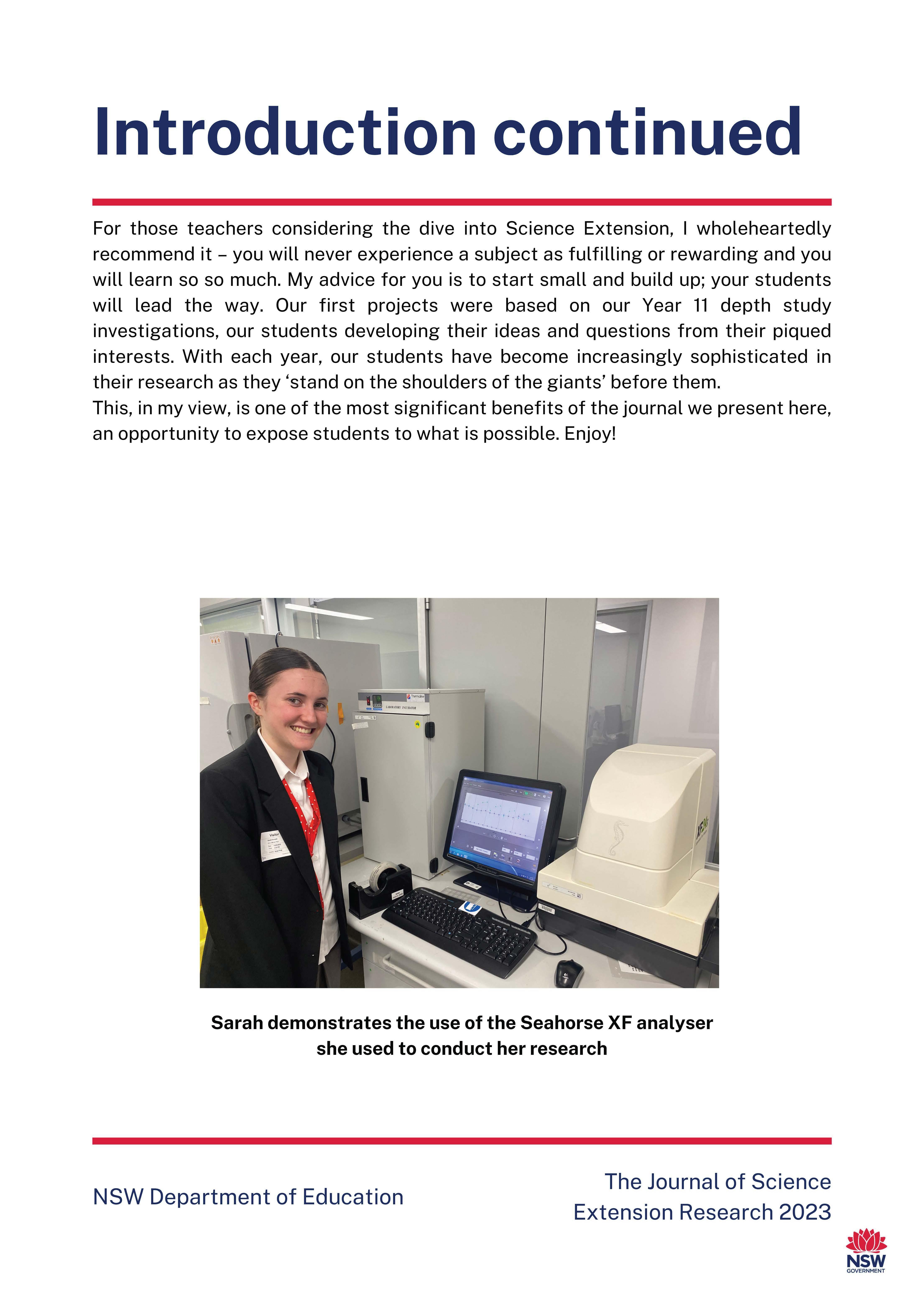
Sarah demonstrates the use of the Seahorse XF analyser she used to conduct her research
In this edition
This edition includes research reports from Science Extension students who completed the course in 2022. All reports are the work of students studying in NSW public schools. They have been supported by their teachers and schools, and in some cases, external mentors.
Running Away from Cancer: An investigation into the dynamic metabolism of cancer cells under an increase in extracellular lactate concentration
This experiment aimed to investigate how a cumulative increase in extracellular lactate affects the ability of a cancer cell line to switch from aerobic glycolysis to oxidative phosphorylation. It was found when the total lactate injected into the cancerous cell line was 15mM and 20mM, there was a significant increase in oxygen consumption rate compared to basal measurements. This suggests that an increase in extracellular lactate does cause cancer cells to shift to an oxidative phenotype in vitro , however further investigations involving a larger sample size and in vivo models are pivotal in assessing the role of lactate, and potentially exercise, in the metabolic processes of cancer.
Bioaccumulation Of Microplastics And Their Respective Chemicals Within Seafood Of Different Trophic Levels: A Meta Study
Secondary data was examined to determine if there is a relationship between the trophic level of ocean species and their bioaccumulation of microplastics. Results show that lower trophic levels are more susceptible to microplastic consumption. This suggests that if humans want to avoid microplastic consumption, they should avoid filter feeders (muscles, oysters, scallops etc.), deposit feeders (bass, eels, crabs etc.) and grazers (lobsters, shrimp etc.).
Flynn Croaker - Coffs Harbour Senior College pp 34-48
Testing The Effect Of Environmental Conditions On Photosynthesis Production
An investigation into the effect of temperature, light availability and chlorophyll concentration on the rate of photosynthesis in plants was undertaken. Higher temperatures, light intensity and chlorophyll concentration were found to increase the rate of photosynthesis.
49-61
Sarah Arnold - Menai High School pp 19-33
Journal of Science
2023 .t'1k NSW GOVERNMENT
Lena Dayil - Lurnea High School pp
The
NSW Department of Education Extension Research
In this edition
Comparing the efficacy of approved TNF-a inhibitors and the emerging field of JAK inhibitors in the treatment of Crohn's Disease
This study investigated and compared the efficacy of TNF-a inhibitors, the standard treatment for Crohn's Disease with JAKinhibitors, an emerging field of biologies. It was found that some JAK inhibitors did not induce a significant difference in clinical or endoscopic remission and the clinical development of one was discontinued, which failed to contend with TNF-a inhibitors which were reliable for safety, clinical and endoscopic remission. This study was significant as it provides CD patients and healthcare professionals with a comparison between the two classes of inhibitors to assist them with their treatment options.
62-84
The impacts of eye drop storage conditions on the microbial growth of eye surfaces

This study aimed to investigate how differing storage conditions of over-the-counter eye lubricants affected the microbial contamination on eye surfaces. It was found that there was a very strong positive correlation between storage conditions and microbial growth on the eye surface. This shows that the correct storage of eye drops is important in preventing or limiting microbial growth on the patient's eye surface.
Effect of 2019-2020 Currowan Bushfires on the Distribution and Populations of Frog Species
This paper investigates the impacts of the Currowan bushfires on the distribution and populations of frog species with reference to both intimate localised sites and the entirety of NSW. The findings concluded that all species' recordings decreased during the fire period, and many increased after the fire period. The impact of fires on frog species is scarcely researched, and it would be highly beneficial for frog conservation and future predications in the light out climate change.
101-113
Chaemin Joseph Kim - James Ruse Agricultural High School pp
Rosie Kerruish - Willoughby Girls High School pp 85-100
night one night two night three
Number of Potential Species -i
11 I.
locations
The Journal of Science NSW Department of Education Extension Research 2023 .t'1k NSW GOVERNMENT
Darcy Kneeshaw- Ulladulla High School pp
In this edition
The Effect of Shrub Layer Composition on Bird Abundance and Species Richness in Revegetation plantings in Hilltops NSW
This study examines how the composition of the shrub layer within revegetation plantings affects species richness and abundance of birds. While areas with high shrub density did not have higher bird abundance, the investigation did show that brid abundance increased with increasing tree dens i ty. It is therefore important to maintain existing areas of established and mature native trees for the benefit of birds.
pp114-124
Investigating the effects of paragraphing and notetaking on memory recall and retention
In this study the effect of paragraphing and note taking format on the recall of information was investigated. The results showed that the presence of notes was significant and the interaction between notes and textual format, varied through paragraphing , was also significant. This holds practical value for the improvement of the study habits of students, could be used in taking down key information from presentations , speeches and interviews and for improving recall driving more informed decision making in workplaces.
Evolutionary Rate Dynamics of SARS-Cov-2 Variants of Concern Throughout the Covid-19 Pandemic
An investigation of how the evolutionary rate of SARS-Cov-2 has varied throughout the pandemic shows that there is long, but temporary, period of rate acceleration around 1.5 times above the mean rate in the Alpha, Gamma and Omicron variants. These results reflect the importance of large genomic datasets built upon global genet i c surveillance efforts in the understanding of the evolutionary dynamics of SARS-Cov-2 which allow for informed public health decisions.

NSW Department of Education
pp 134-144
The Journal of Science
Extension Research 2023
8 • 6 • • 4 ' • 2 • • 0 5000 10000 15000 20000 Shrubs per ha
Hannah Southwell - Boorowa Central School
!= No te tabngfo mat
Blacktown Girls High School
Alexandra Vergel de Dios - pp 125-133
- ~F'i"_ ; -, 11\~· ~ -:.
Owen Yi - James Ruse Agricultural High School
.t'1k NSW GOVERNMENT
In this edition
A Comparison of the Concentration of Lycopene in Australian and Italian Canned Tomatoes
This study aimed to determine if there is a difference in the concentration of lycopene, a powerful antioxidant, in tinned tomatoes from Australia and Italy. The lycopene concentration of canned tomatoes from Italy and Australia was not significantly different. Consuming foods and meals made with tomatoes sourced locally or from Italy will provide the same amount of lycopene and thus the same antioxidant properties and health benefits.
pp 145-155
How The Anomalous Behaviour of Hydrogen Fluoride Provides
Into
The anomaly behind the weak acid nature of hydrofluoric acid has sparked scientific discourse for nearly a century, with the most recent explanation accounting a lack of ionisation to entropic factors. This report extrapolates the theorised principle by establishing causation between hydration entropy of a wide array of monoprotic acid anions and their tendency to ionise in an aqueous system. It was found that an increased hydration entropy of monoprotic anions is directly related to a decreased tendency of the acid to ionise in an aqueous solution.

Plant Power vs the Water World: An Insight into the Detoxifying Properties of Typha Orientalis in Polluted Water
This investigation explored the detoxifying and filtrating properties of Typha Orientalis, a wetland plant, in the removal of Copper (11) Sulfate and Cooking Oil in water - to simulate pollutants found in Sydney Harbour. This experiment provided quantitative and qualitative data to support the application of Typha Orientalis in the filtration of polluted water in the real world, ultimately to reach a safe level of contaminants fit for consumption as deemed by World Health Organisation
pp172-189
Jacob Hill -St. Ives High School
Insight
The
of
• • Mogrnludc of I lydrallon entropy, pKo (, ,o homologom, groups) 10 0 "' 10
Nature
Ionisation
Theo Mortazavi - Normanhurst Boys High School pp 156-171
Elena Mbeya - Menai High School
The Journal of Science NSW Department of Education Extension Research 2023 .t'1k NSW GOVERNMENT
In this edition
Meta-study of the ability of seaweed farms to locally mitigate ocean acidification
This meta-study used secondary sourced data to test whether seaweed farms had the ability to locally mitigate ocean acidification. It was found that the pH of seaweed farms was higher than the control sites without seaweed farms. Ocean acidification causes calcifying organisms' skeletons to become susceptible to dissolution, so any activity that could reduce ocean acidification would be beneficial, however more long term studies need to be undertaken to determine for how long and how widespread the effects of the seaweed farms are.
Characterisation of the Chaotic Behaviour of a Simple Two-Transistor Single-Supply Resistor-Capacitor Circuit
The claims of chaotic behaviour in a circuit were investigated through utilising both in-situ and in-silica solutions. The validity of the simulation was confirmed as chaotic behaviour was observed in the in-situ circuit. The proposed chaotic circuit utilised cheap and readily available parts, hence, there is scope for its implementation in areas such as robotics or encryption, where chaos greatly increases efficiency and effectiveness.
The Effectiveness Of Different Sound Absorbing Materials On The Transmission Of Sound At 3000 Hz
This investigation aimed to determine which sound absorbing material (concrete sheets, plaster sheets, acoustic pinboard and Abel flex Expansion Joint Filler) prevents transmission of sound when tested at a frequency of 3000 Hz. Acoustic pinboard was found to be the most effective in preventing sound transmission. This product would be most useful for controlling sound levels for environments like offices or sound rooms.
1$ 11.ZO ~ II '=-s..oo "' 91 .M$ ,...._ _ - Farm
Leroy Van Schellebeck - Coffs Harbour Senior College pp190-197
James Harrison - Lambton High School pp 198-211
Journal of Science
Department of Education Extension Research 2023 .t'1k NSW GOVERNMENT
Eelan Al Zuhairi -Lurnea High School pp 212-227
The
NSW
In this edit 10n
Disproving The Misconception That Microscopic Black Holes Can Expand
This derivation of Hawkins equations using dimensional analysis and observing the relationship between the variables of mass and time refutes the common misconception that a microscopic black hole produced in a supercollider can expand and absorb matter until it grows to the size of a cosmic black hole. The impact of this area of research can lead to new discoveries and development of technologies that will advance our knowledge and understanding of the universe.
pp 228-239
Data Samples
Predicting Solar Proton Event Magnitudes Using Vector Magnetic Data and a Neural Network
Ta rgets
This study aimed to create and evaluate a neural network using vector magnetic data to predict the maximum proton flux at Earth caused by a future solar proton event (SPE). By analysing the ratio of underestimations to overestimations and comparing the error of the predictions made by these neural networks to the corresponding errors for baseline models with no skill, it was evident that neither neural network would be accurate enough to be used in a real-life scenario to alert authorities to a strong SPE likely to impact technologies and humans
pp 240-256
Analysis of Properties of Transition Disk Post-A GB Binary Systems for Planet Formation
This work aims to analyse if properties such as chemical abundances of the post-Asymptotic Giant Branch star may correlate with planet occurrence established by previous photometric analysis. Planet-containing galactic post-AGB binaries were found to exhibit higher median elemental abundances but lower metallicities ([Fe/HJ) than the population
The post-AGB sample disobeys the PMC that characterises 1stgeneration planet forming stars likely due to the very different mechanisms behind disk and planet formation but further research is needed to determine the exact processes involved.
pp 257-276
} ... • I
I
Surabhi Hebbar - Blacktown Girls High School
Vincent Ng- James Ruse Agricultural High School
... f' I ,oo ... ... ... .. ... ......... ____ -,-_..._.,...- _, _ ...,,
Yi Wei Yang- James Ruse Agricultural High School
The Journal of Science NSW Department of Education Extension Research 2023 .t'1k NSW GOVERNMENT
In this edition
Number of Rising Sequences of the Riffle and Overhand Card Shuffles
An experimental study examined the number of rising sequences of the rifle and overhand shuffling strategies. No significant difference was found between the two strategies. Future directions for experimentation could compare the randomness between the riffile and overhand manual shuffling practices with a mechnical shuffle.
277-288
Segmenting Lungs Under Adverse Conditions Using Multi-Stage Transfer Learning: Preliminary Evidence of the Increased Generalisability when Retraining on Flipped Datasets
This performance of multi-stage transfer learning (MSTL) on a lung segmentation task within adverse conditions was investigated. It was concluded that most of the retrained models likely experienced covariate shifts with the exception of models trained on flipped datasets. This investigation gives insight into the thresholds of models trained on small datasets to perform under adverse conditions, adding to the knowledge base required to successfully integrate deep learning (DL) into the medical workflow.

Rmn a St-Q~ocnofR1ffkandChtrhand Card huffin - Ro nlt "hi l~ ,.,...,..,,."""'k
Leonardo Bruzze - Cherrybrook Technology High School pp
The Journal of Science NSW Department of Education Extension Research 2023 .t'1k NSW GOVERNMENT
Minalu de Graaf- Lambton High School pp 289-302
Running Away from Cancer: An investigation into the dynamic metabolism of cancer cells under an increase in extracellular lactate concentration
Sarah Arnold Menai High School
A distinctive hallmark of cancer cells is a high glucose uptake and lactate production regardless of oxygen availability, known as the Warburg Effect. Emerging studies suggest the Warburg Effect could be counteracted by increasing extracellular lactate concentration, which could occur during anaerobic exercise, however research is scarce. This experiment aimed to investigate how a cumulative increase in extracellular lactate affects the ability of a cancer cell line to switch from aerobic glycolysis to oxidative phosphorylation (OXPHOS) through measuring extracellular acidification rate (ECAR) and oxygen consumption rate (OCR) respectively, using advanced Seahorse XF technology. It was found when the total lactate injected into the cancerous cell line was 15mM and 20mM, there was a significant increase in OCR compared to basal measurements, where P=0.00301 and P=0.000686 respectively. This suggests that an increase in extracellular lactate does cause cancer cells to shift to an oxidative phenotype in vitro, however further investigations involving a larger sample size and in vivo models are pivotal in assessing the role of lactate, and potentially exercise, in the metabolic processes of cancer.
Literature Review
Cancer is the leading cause of death worldwide, responsible for approximately 10 million deaths in 2020 (WHO, 2021). Additionally, it is estimated that ¼ of adults worldwide do not achieve sufficient amounts of physical exercise (Mathewson, 2018). Alarming, emerging studies suggest an intertwine between these global issues, indicating that lactate resulting from single bouts of exercise may have a direct effect on tumour intrinsic factors (Dethlefsen, 2017, Hofmann, 2018).
Cancer cells: An unusual metabolism
Noncancerous cells rely primarily on oxidative phosphorylation (OXPHOS) to generate approximately 70% of their ATP for cellular processes. One fuel for OXPHOS is pyruvate, the end product of the enzymatic breakdown of glucose, known as glycolysis (Ristow, 2006). Under aerobic conditions, pyruvate is transported to the mitochondria where it is oxidised to acetyl-CoA. Acetyl-CoA is further combined with oxaloacetate to initiate the tricarboxylic acid (TCA) cycle, leading to OXPHOS and resulting in the synthesis of ATP energy (Zheng, 2012).
Discovered by Otto Warburg (Warburg et al., 1927), a hallmark of cancerous cells is an accelerated glycolytic metabolism to
The Journal of Science Extension Research – Vol. 2, 2023 education.nsw.edu.au 19
convert glucose to lactate rather than through OXPHOS, even under fully oxygenated conditions (San-Millán and Brooks 2017). This theory has been supported by various studies (Fadaka et al., 2017, Hirschhaeuser et al., 2011, Jose et al., 2010, Ruiz et al., 2009, SanMillán and Brooks, 2017, Zheng, 2012) and is known as the Warburg Effect or aerobic glycolysis. This phenomenon has remained a mystery across scientific literature, as glycolysis appears inefficient to cancer cells, yielding only 2 ATP molecules, compared to 40 ATP molecules generated by OXPHOS (Fadaka et al., 2017). Consequently, cancerous cells demand a high glucose consumption to maintain homeostasis (Hanahan & Weinberg, 2011).
Whilst previous literature accepts the Warburg Effect is a consequence of defects in cellular respiration, oncogenic alterations, and an overexpression of glycolytic enzymes and metabolite transporters (Hirschhaeuser et al., 2011), the underlying mechanisms of Warburg Effect in cancer cells has been unknown for nearly a century. This may be partially due to an unparalleled focus on genomic techniques in cancer research over the recent decades, which has resulted in a neglected understanding of cancer metabolics (Hofmann, 2018). However, it was recently proposed that the purpose of the Warburg Effect is solely lactate production, known as lactagenesis (SanMillán and Brooks, 2017), implying its role beyond a waste product. During lactagenesis, pyruvate is reduced into lactate, catalysed by the enzyme lactate dehydrogenase (LDH) (Xie et al., 2014), and this reaction is reversible (Mishra and Banerjee, 2019). However, limited studies have accounted for the reversible nature of this equilibrium reaction, in regards to
the underlying mechanisms of the Warburg Effect.
Challenging the Warburg paradigm
Building on Warburg’s model, the Reverse Warburg Effect proposes that not all cancer cells undergo aerobic glycolysis, but rather lactate is shuffled and used as an energy source from cancer-associated fibroblasts (CAFS) via monocarboxylate transporters (MCTs) (Wilde et al., 2017). This is supported by the findings that tumours are not exclusively hypoxic, but rather contain aerobic regions which receive shuttled lactate from other glycolytic cancer cells (Semenza, 2008). The Reverse Warburg Effect induces localised lactic acidosis in the tumour microenvironment (TME) causing an accumulation of lactate (Siska, 2020) and due to the high ionisation of lactic acid, a consequent decrease in pH which may favour metastasis, angiogenesis and immunosuppression (de la Cruz- Lopez et al., 2019) and potentially chemoresistance (Brown et al., 2019). However, it is important to note that cancers are extremely heterogeneous with individual metabolic features (Zheng, 2012, Semenza, 2008), potentially limiting the application of Reverse Warburg Effect.
It has also been outlined that the transport of lactate into cancer cells through MCTs is dependent on a concentration gradient (Hofmann 2018, Payen et al., 2019) in order to avoid intracellular acidification (Brown et al., 2019). In 2018, Hofmann further hypothesised if the blood lactate concentration surrounding the tumour can be increased, for example through exercise, this could inhibit the shuttling of
The Journal of Science Extension Research – Vol. 2, 2023 education.nsw.edu.au 20
lactate and hence the process of the Reverse Warburg Effect. However, it was necessitated by Hofmann that there is extremely limited research on the mechanisms of single bouts of exercise on cancer.
Reverting the Warburg Effect?
The shift of energy metabolism from OXPHOS to aerobic glycolysis has now been widely accepted as a quintessential feature of cancer (Hanahan & Weinberg, 2011). In 2016, Wu inquired if cancer cells can revert from the Warburg effect to OXPHOS when induced by TME pressures. Wu’s results concluded without lactic acidosis, glycolysis and OXPHOS provided 23.7% - 52.2% and 47.8% - 76.3% of total ATP generated, respectively; whilst with lactic acidosis, glycolysis and OXPHOS provided 5.7%13.4% and 86.6% - 94.3% of total ATP generated respectively. This suggested lactic acidosis could revert cancer cells from the Warburg to the OXPHOS phenotype. Furthermore, it has been demonstrated, when 4T1 cancer cell lines were induced with lactic acidosis the cells showed a non-glycolytic phenotype characterised by a high oxygen consumption rate over glycolytic rate, negligible lactate production and efficient incorporation of glucose into cellular mass, revealing the dual metabolic nature of cancer cells (Xie et al., 2014).
However, Wu’s study induced the switch between glycolysis and OXPHOS using inhibitors (oligomycin, FCCP, Rotenone/ AntimycinA), and no research appears to stimulate this metabolic switch by increasing extracellular lactate. The study conducted by Wu in 2017 was also the first to quantitatively measure such a metabolic switch and only studied cell
lines in two conditions (lactic acidosis and a control group). Therefore, such metabolic switch has not been investigated under varying concentrations of lactate as a means to model the accumulation of lactate as demonstrated in anaerobic exercise. This metabolic switch was also hypothesised by SanMillán and Brooks in 2017, who suggested that aerobic exercise could contribute to counteracting such switch to a glycolytic metabolism in cancer cells by creating epigenetic responses to restorate oxidative phenotypes, however, experimentations have been conducted.
It has been further suggested, if glycolysis could be inhibited in cancer cells, OXPHOS could be restored (Zheng, 2012). This is supported by the increasing number of studies that reveal lactate released by glycolysis and/or CAFS is not discharged as cellular waste, but rather is taken up by oxygenated tumour cells as energy fuel. It has been proposed that this occurs as lactate is converted to pyruvate by LHD where it enters the mitochondria and undergoes OXPHOS (Zheng, 2012). Limited studies however investigate the implications of adding the product, i.e. lactate, to this equilibrium as a potential mechanism for lactic acidosis causing the apparent shift from glycolysis to OXPHOS. However, it was noted that circulating lactate levels are critical in dictating the status of the LHD equilibrium, and Wu in 2014, concluded no net lactate generation was due to the equal rate of pyruvate generated from glycolysis with the removal into the TCA cycle (Xie et al., 2014). However, these concepts are mechanistic explanations of the Warburg Effect, which have yet to be justified by experiment.
The Journal of Science Extension Research – Vol. 2, 2023 education.nsw.edu.au 21
A potential model for the effects of exercise on cancer
Despite a history of lactate being defined as only a waste product, over the last decade research has revealed lactate produced by exercise is an active metabolite, moving between cells and capable of being oxidised as a fuel (Philp, et al., 2005). Currently, there is limited research on the intrinsic effects of exercise on cancer cell metabolism. Exercise unquestionably has a role in regulating metabolic processes, but how this consequently affects tumour growth and metastatic rate is not currently mechanistically understood (Hojman, 2018). A study by McTiernan suggested physical activity may be linked to cancer production through exercise-dependent reductions in cancer risk factors; including sex hormones, insulin growth factor (IGF), inflammatory markers and improving immune function. The large inconsistencies regarding the exercise dose which is ideal for cancer management in current research with reference to intensity, duration, frequency and type hinders compelling conclusions (Ashcraft, 2016).
Therefore, cancer cell research demands quantitative over qualitative studies to meet the increasing prevalence of disease. Lactate holds promise to play a role in cellular properties beyond purely a waste product (San-Millan, 2017). Therefore, investigations in the role of lactate on cancer cells in vitro, could provide insight into a further understanding of the potential benefits, or risks, of exercising for cancer patients.
Scientific Research Question:
Will increased extracellular lactate concentrations in a cancerous cell line
cause a change in the extracellular acidification rate (ECAR) and oxygen consumption rate (OCR)?
Scientific Hypothesis:
The cancerous cell line exposed to increased lactate concentrations is expected to increase in OCR and decrease in ECAR. This is supported by studies which propose that lactic acidosis can revert glycolytic cancer cells to a dominant oxidative phenotype (Dethlefsen, 2017, Hofmann, 2018, Nijsten & van Dam, 2009, San-Millán & Brooks, 2017, Wu et al., 2016).
Methodology
The investigation consisted of measuring extracellular acidification rate (ECAR) and oxygen consumption rate (OCR) in a cancerous cell line 4T1 (ATCC) at differing concentrations of sodium lactate using the novel Seahorse Extracellular Flux 24 (XF) analyser (Seahorse Bioscience). Sodium lactate was injected to the medium at cumulative increments from 0mM to 20mM (0mM, 5mM, 10mM, 15mM, 20mM) through integrated injection ports. In the control sample, a buffered serum, without lactate, was injected at the same concentrations and increments as the lactate group. This technology was specifically selected due to its dual ability to provide an indication of glycolysis and OXPHOS by measuring ECAR and OCR respectively, through real time measurements of changing pH and oxygen concentrations in the extracellular medium.
Glycolysis will be determined through measurements of the ECAR of the surrounding cell media, caused by the excretion of lactate per unit of time after the conversion from pyruvate in cells,
The Journal of Science Extension Research – Vol. 2, 2023 education.nsw.edu.au 22
altering pH (Wu et al., 2006). However since the lactate injected into the cell line also has acidic properties, this will inevitably reduce the validity of glycolysis measurements by altering pH levels which may not reflect the metabolic measurements of the cells. Therefore this justifies the selection of the Seahorse technology which has the ability to measure oxygen consumption rate, which is calculated by oxygen concentration (Plitzko et al., 2017) and therefore will not be influenced by lactate injections.
Prior to the assay, the cells were stored in a biosafety cabinet II at 37oC and 5% CO2 to effectively replicate conditions of the human body. Both cell lines were cultured in a low glucose Dulbecco’s modified Eagle’s medium (DMEM) containing 10% fetal bovine serum (FBS) as well as other nutrients to control cell growth. 10 wells of the Seahorse XF 24 well microplate were each filled with approximately 10 000 cells of the cancerous 4T1 cell line and 10 remaining wells were likewise filled and allocated as the control. 4 wells were left blank as a control for the machine and the cells were left in the biosafety cabinet (37oC, 5% CO2) overnight. Prior to the assay the next morning, the cancerous cells were examined and observed under the microscope to monitor any abnormalities (Appendices 1).
The microplate was placed into the Seahorse XF and 3 basal measurements of ECAR and OCR were recorded with 0mM lactate. The assay then recorded 15 measurements for each of the 20 wells, recording ECAR and OCR rates at each time increment. Between each measurement the cells were mixed during a 5 minute cycle. Lactate concentration was cumulatively increased and 3
measurements were recorded for each concentration increment in each well. The same procedure was completed for the control, with the buffer solution injected.
Ethical and biosafety considerations have been addressed by the completion of the experiment to be conducted at Garvan Institute of Medical Research, where the hazardous and cancerous cell lines were stored in a Biosafety cabinet II and under appropriate conditions and protocol.
Results and analysis:
Null hypothesis:
As extracellular lactate cumulatively increases, the rates of extracellular acidification rate and oxygen consumption rate will not change as extracellular lactate concentration has no influence on cancer cell metabolism.
Alternative hypothesis H1:
As extracellular lactate cumulatively increases, the rates of extracellular acidification rate and oxygen consumption rate will change as extracellular lactate concentration has an influence on cancer cell metabolism.
The Journal of Science Extension Research – Vol. 2, 2023 education.nsw.edu.au 23
Inferential statistical analysis:
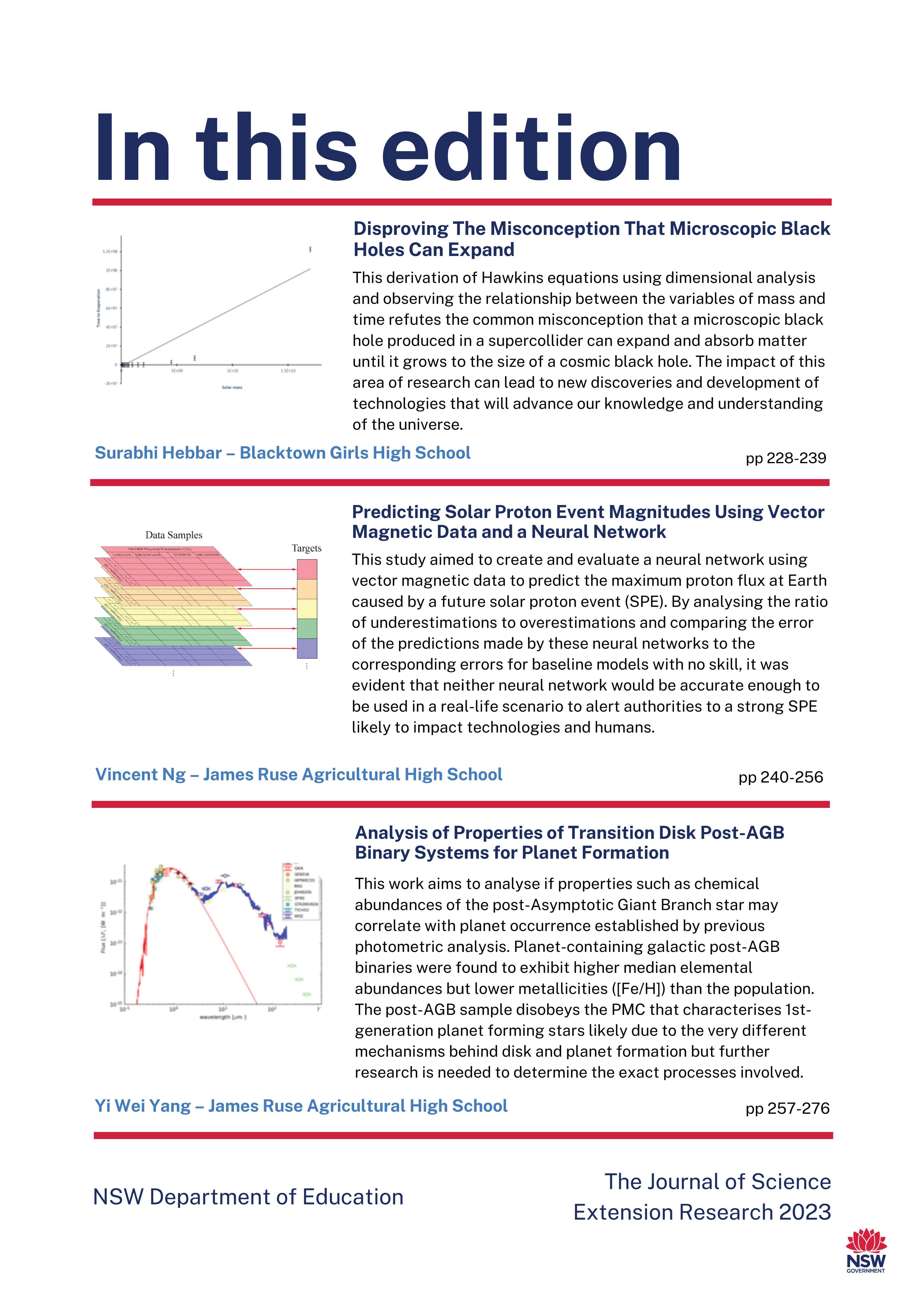
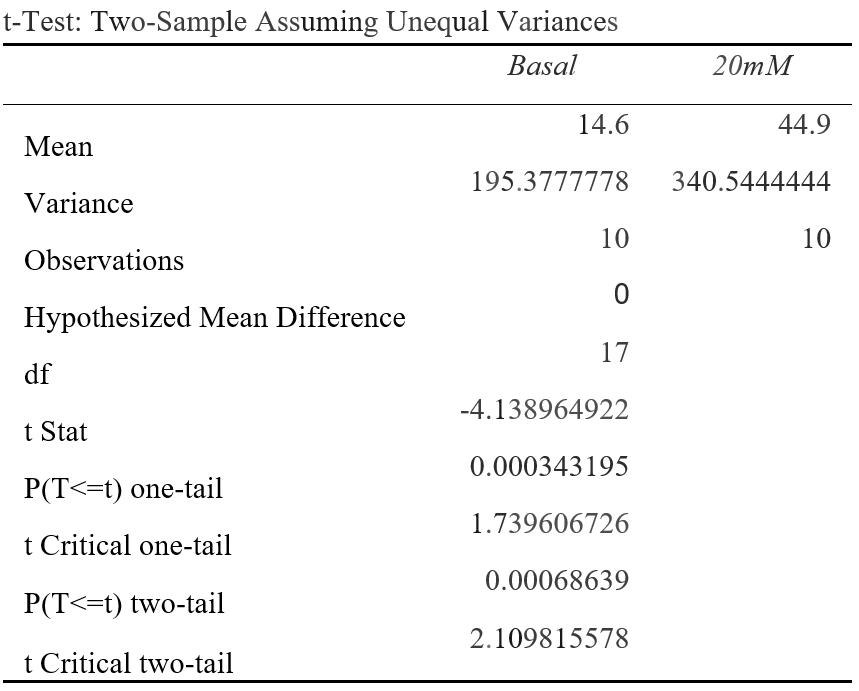
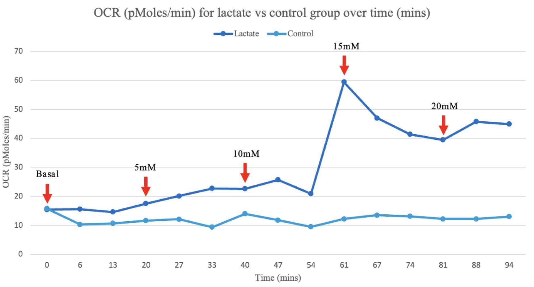
Unpaired, student t-tests were applied to determine if there was a statistical significance for each increment of lactate (5mM, 10mM, 15mM, 20mM) compared to basal measurements for both ECAR and OCR rates. The alpha value was set to p=0.05, meaning any values that were more than 5% due to chance, were deemed insignificant. The same t-tests were conducted for the control with the addition of a buffered solution. All p values for the control were insignificant (p > 0.05) and ranged from p=0.98 to p=0.40. Significant differences were measured at 15mM (Figure 1A) and 20mM for OCR (Figure 1B) and at 5mM (Figure 2A), 10mM (Figure 2B), and 20mM (Figure 2C) for ECAR.

Statistical analysis of lactate group for OCR measurements:
Figure 1B: P(T<=t) two-tail = 0.000686 (P<0.05) OCR (pMoles/min) was measured at a basal rate (13mins) and when 20mM was injected to the cell line (94mins). The difference between the average OCR for cancer cells at basal rates compared to 20mM were statistically significant as the results were 0.00686% due to chance. This suggests that 20mM of lactate could affect OCR.

Statistical analysis of lactate group for ECAR measurements:
Figure 1A: P(T<=t) two-tail = 0.00301 (P<0.05) OCR (pMoles/min) was measured at a basal rate (13mins) and when 15mM was injected to the cell line (74mins). The difference between the average OCR for cancer cells at basal rates compared to 15mM were statistically significant as the results were 0.0301% due to chance. This suggests that 15mM of lactate could affect OCR.
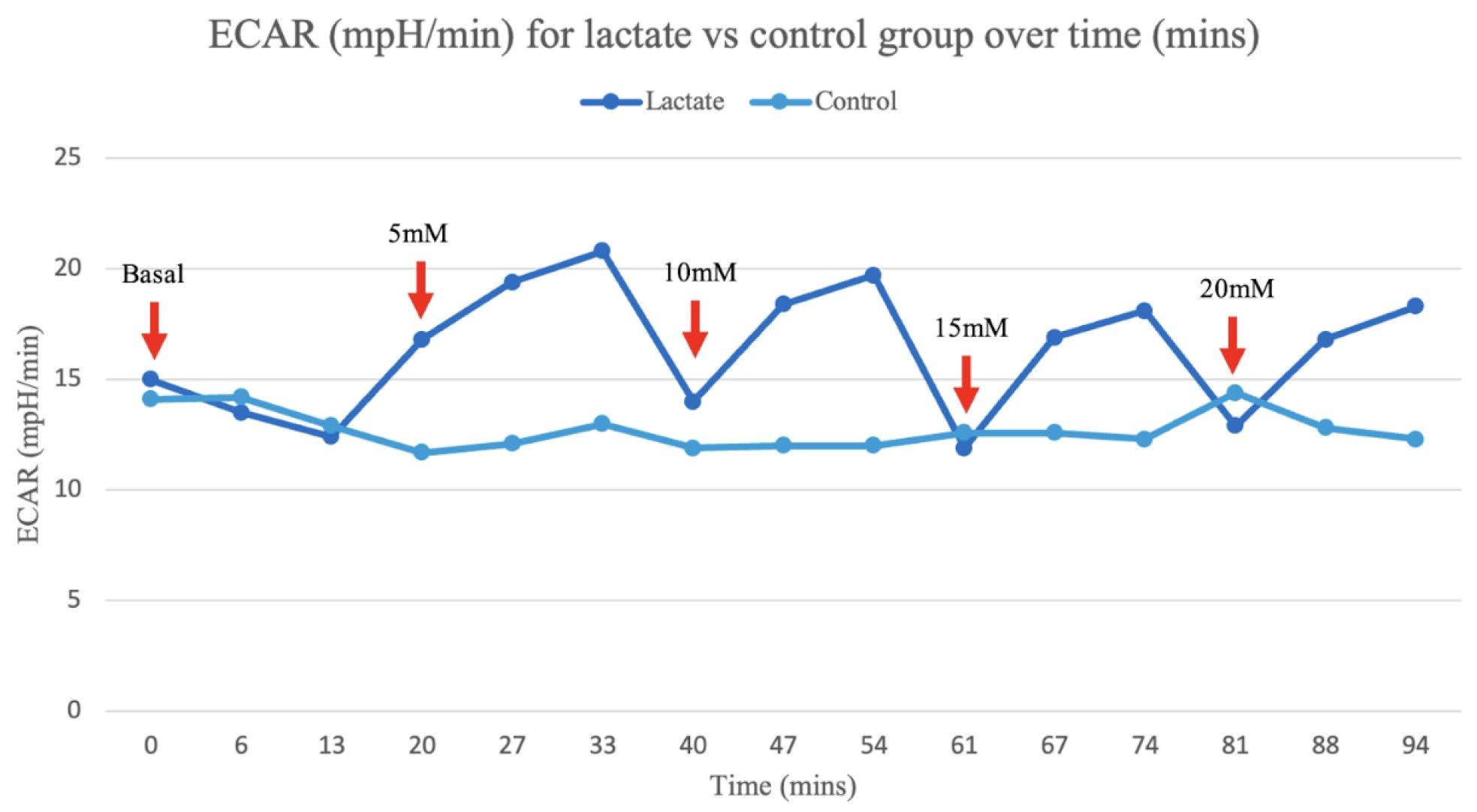
Figure 2A: P(T<=t) two-tail = 0.0128 (P<0.05) ECAR (mpH/min) was measured at a basal rate (13mins) and when 5mM was injected to the cell line (33mins). The difference between the average ECARfor cancer cells at basal rates compared to 5mM were statistically significant as the results were 1.28% due to chance. This suggests that 5mM of lactate could affect ECAR.
The Journal of Science Extension Research – Vol. 2, 2023 education.nsw.edu.au 24
Figure 2B: P(T<=t) two-tail= 0.0294 (P<0.05) ECAR (mpH/min) was measured at a basal rate (13mins) and when 1 0mM was injected to the cell line (54mins). The difference between the average ECAR for cancer cells at basal rates compared to 10mM were statistically significant as the results were 2.94% due to chance. This suggests that 10mM of lactate could affect ECAR.

Descriptive statistical analysis:
Descriptive analysis for OCR measurements:
Figure 2C: P(T<=t) two-tail= 0.0337 (P<0.05) ECAR (mpH/min) was measured at a basal rate (13mins) and when 20mM was injected to the cell line (94mins). The difference between the average ECAR for cancer cells at basal rates compared to 20mM were statistically significant as the results were 3.37% due to chance. This suggests that 20mM of lactate could affect ECAR.
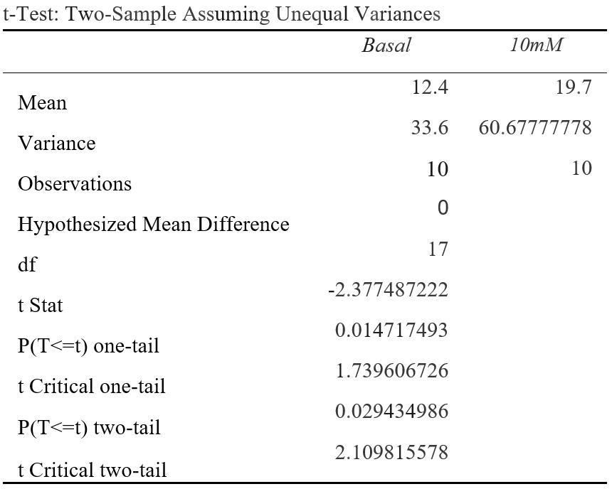
Figure 4A: The average OCR measurements were calculated for the lactate and control group for each time interval during the assay.
The Journal of Science Extension Research – Vol. 2, 2023 education.nsw.edu.au 25
Figure 4B: The average OCR measurements for the lactate and control group were graphed for each recorded time interval. The red arrows signify the point at which 5mM of lactate was cumulatively injected.
Descriptive analysis for ECAR measurements:
Figure 5A: The average ECAR measurements were calculated for the lactate and control group for each time interval during the assay.
The Journal of Science Extension Research – Vol. 2, 2023 education.nsw.edu.au 26
Discussion:
The T-tests conducted reveal lactate has a significant effect on the rates of ECAR and OCR at various concentrations when compared to basal measurements. For the independent group of cancerous cells, significant differences between the means (p<0.05) of the basal rate when compared to the interval at a set concentration (5mM, 10mM, 15mM or 20mM) suggested lactate had a profound effect on either ECAR or OCR measurements as there were a less than 5% likelihood that results were obtained by chance. This occurred at intervals
15mM (p=0.00301) and 20mM (p=0.000686) for OCR measurements
(Figure 1A and B), and at 5mM (p=0.0128), 10mM (p=0.0294) and 20mM (p=0.0337) for ECAR measurements
(Figure 2A, B and C). For the control group of cancerous cells, which were injected with a buffer serum without lactate, all p-values were high ranging
from p=0.404 to p=0.975. This indicates that there were most likely no confounding variables significantly influencing the results, and lactate was the source of change in the experiment. Therefore, the null hypothesis that lactate does not change the ECAR and OCR measurements in a cancerous cell line can be rejected in favour of the alternate hypothesis.
An average of the independent samples indicated ECAR measurements increased over the 5 minute cycle period following an increase in lactate concentration at 13, 40, 61 and 81 minutes, then returned to a similar rate, despite the cumulative increase in extracellular lactate concentration (Figure 5B). This is most likely due to the acidic properties of the sodium lactate added causing anomalous results as ECAR measurements are dependent on pH, evident in the significant increase in ECAR at 5 and 10mM increments (Figure 2A and B).
Figure 5B: The average ECAR measurements for the lactate and control group were graphed for each recorded time interval. The red arrows signify the point at which 5mM of lactate was cumulatively injected.
The Journal of Science Extension Research – Vol. 2, 2023 education.nsw.edu.au 27
However, the OCR measurements, which are calculated from moles rather than pH, suggest that as lactate concentration increases the rate of OCR also increases, evident in the spike in the rate of OCR in the independent group after 54 minutes when compared to the control (Figure 4B).
The evident switch in the cancerous cell line to a more oxidative metabolism when an accumulation of lactate injected was 15mM and greater, corresponds with emerging literature in the field and reitarties the importance of lactate in understanding cancer metabolics (Wu et al., 2016). The significant increase in OCR in the independent group at 15mM (p=0.00301) from 14.6 to 41.4 pMoles/min and at 20mM (p=0.000686) from 14.6 to 44.9 pMoles/min, provides a point at which lactate causes a metabolic switch from aerobic glycolysis to OXPHOS, extending from current scientific literature (Wu et al., 2016).
Current literature proposes that glycolytic cancer cells are able to sustain their metabolism through types of lactate shuttling including the Reverse Warburg Effect, metabolic symbiosis and vascular endothelial growth (Kooshki et al., 2021), as not all cancer cells necessarily produce lactate (Semenza, 2008). The increase in an oxidative metabolism from 15mM of lactate could therefore be due to disruption of the lactate shuttling concentration gradient required to transport lactate through MCTs, causing the cancer cells to rather use lactate as a fuel for oxidation, potentially indicated by the decrease plateau of OCR from 61 minutes onwards (Figure 4B). The increase in OCR at 15mM could also be attributed to an increase in lactate favouring the oxidation of lactate to
pyruvate via LDH, resulting in pyruvate to be used as fuel for OXPHOS (Xie et., 2014). The increase in OCR could also be due to the increase in extracellular lactate decreasing the efficacy at which glucose can diffuse into GLUT transporters in glycolytic cells, creating an environment where glycolytic cancer cells adapt by increasing OCR.
Key limitations and future directions for scientific research:
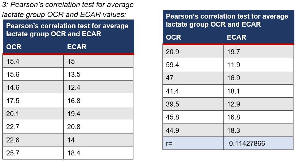
The in vitro nature of the experiment was beneficial for providing quantitative data on a cellular level for the effects of lactate on cell metabolism, however is limited in providing a thorough understanding of the role of lactate in vivo. The variation across each individual assay (Appendices 2), highlights the need for further replications to analyse results with a large variance to mirror the diversity of ways heterogeneous cancer cells may react under experimental conditions. Despite the highly advanced Seahorse XF technology, it is limited as during the mixing phase of each cycle during the assay, as there is potential that cells could have broken off, impacting the cell count and the reliability of the results. The Seahorse XF results also indicated on various occasions 0 values for either ECAR and OCR (Appendices 2) which also limits the validity of the results as it is questionable if the cells are ever at a state of 0. The limitations of using lactate as the independent variable, which affects pH measurements, also impacts findings as no noticeable trend was observed from ECAR measurements, which could further suggest why there was an insignificant Pearson's correlation coefficient (r=-0.114) between the two measurements (Appendices 3).
The Journal of Science Extension Research – Vol. 2, 2023 education.nsw.edu.au 28
Whilst the experiment provided insight to the role of lactate on a cellular level, it cannot be concluded that this directly mirrors the role of exercise, which also produces lactate, on cancer cells. Whilst the concentrations of lactate in the experiment mirror the concentration produced during exercise, further research is required to understand how lactate is transported to tumours from a bodily perspective to assess the accuracy of this experiment as a potential model. Further experimentation should be conducted with a larger sample size over multiple occasions, as well as comparing the results with a noncancerous cell line to further scientific understanding.
Investigations into quantitative, in vivo experiments for the role of lactate on glycolysis and OXPHOS will also be beneficial in order to understand the role of single bouts of exercise on tumour intrinsic factors.
Conclusion:
A clear increase in OCR when lactate injected cumulated to 15mM and 20mM, where P=0.00301 and P=0.000686 respectively, indicates a significant link between the concentration of extracellular lactate and the metabolic profile of cancer cells in vitro. Therefore, despite the lack of validity of ECAR measurements due to the addition of lactate potentially impacting the pH of results, it can still be established that an increase in lactate does result in cancer cells switching to a more oxidative phenotype, and the null hypothesis can be rejected in favour of the alternate hypothesis. Hence, these results suggest that lactate could revert the Warburg Effect in cancer cells by potentially disrupting the concentration gradient required for cells to shuttle lactate intercellularly to sustain such a
highly glycolytic metabolism. It is critical that further investigations explore the effects of lactate on cancer cells from an in vivo perspective, in order to determine the effects of single bouts of lactate on cancer cell metabolics, as a means of providing a foundation of the possible mechanisms of the effects of exercise on cancer.
Acknowledgements
I would like to express my gratitude to Dr Andy Philip and Garvan Institute of Medical Research for conducting the experiment and providing the Seahorse XF experimental data. I would also like to thank my teacher Ann Hanna for guidance with the data analysis, and my mentor Clara Zwack from the University of Sydney for their support with contacting academics. I would also like to extend my appreciation to my peer Emily Cliff and chemistry teacher Zoe Liley for their feedback regarding the scientific report.
References: Ashcraft, K. A., Peace, R. M., Betof, A. S., Dewhirst, M. W., & Jones, L. W. (2016). Efficacy and Mechanisms of Aerobic Exercise on Cancer Initiation, Progression, and Metastasis: A Critical Systematic Review of In Vivo Preclinical Data. Cancer Research, 76(14), 4032–4050. https://doi.org/10.1158/00085472.can-16-0887
Brown, T. P., & Ganapathy, V. (2020). Lactate/GPR81 signaling and proton motive force in cancer: Role in angiogenesis, immune escape, nutrition, and Warburg phenomenon. Pharmacology & Therapeutics, 206, 107451.
The Journal of Science Extension Research – Vol. 2, 2023 education.nsw.edu.au 29
https://doi.org/10.1016/j.pharmthera.2019
.107451
de la Cruz-López, K. G., Castro-Muñoz, L. J., Reyes-Hernández, D. O., GarcíaCarrancá, A., & Manzo-Merino, J. (2019). Lactate in the Regulation of Tumor Microenvironment and Therapeutic Approaches. Frontiers in Oncology, 9.
https://doi.org/10.3389/fonc.2019.01143
Dethlefsen, C., Pedersen, K. S., & Hojman, P. (2017). Every exercise bout matters: linking systemic exercise responses to breast cancer control. Breast Cancer Research and Treatment, 162(3), 399–408.
https://doi.org/10.1007/s10549-017-41294
Fadaka, A., Ajiboye, B., Ojo, O., Adewale, O., Olayide, I., & Emuowhochere, R. (2017). Biology of glucose metabolization in cancer cells. Journal of Oncological Sciences, 3(2), 45–51.
https://doi.org/10.1016/j.jons.2017.06.002
Hanahan, D., & Weinberg, Robert A. (2011). Hallmarks of cancer: the next generation. Cell, 144(5), 646–674.
https://doi.org/10.1016/j.cell.2011.02.013
Hirschhaeuser, F., Sattler, U. G. A., & Mueller-Klieser, W. (2011). Lactate: A Metabolic Key Player in Cancer. Cancer Research, 71(22), 6921–6925.
https://doi.org/10.1158/0008-5472.can11-1457
Hofmann, P. (2018). Cancer and Exercise: Warburg Hypothesis, Tumour Metabolism and High-Intensity Anaerobic Exercise. Sports, 6(1), 10.
https://doi.org/10.3390/sports6010010
Hojman, P., Gehl, J., Christensen, J. F., & Pedersen, B. K. (2018). Molecular
Mechanisms Linking Exercise to Cancer Prevention and Treatment. Cell Metabolism, 27(1), 10–21.
https://doi.org/10.1016/j.cmet.2017.09.01 5
Kooshki, L., Mahdavi, P., Fakhri, S., Akkol, E. K., & Khan, H. (2021). Targeting lactate metabolism and glycolytic pathways in the tumor microenvironment by natural products: A promising strategy in combating cancer. BioFactors.
https://doi.org/10.1002/biof.1799
Mathewson, T. (2018, October 30). More than 1 in 4 people across the world don’t get enough exercise, study says. Global Sports Matters.
https://globalsportmatters.com/health/201 8/10/30/over-1-in-4-people-across-theworld-dont-getenough-exercise-studysays/
Mishra, D., & Banerjee, D. (2019). Lactate Dehydrogenases as Metabolic Links between Tumor and Stroma in the Tumor Microenvironment. Cancers, 11(6), 750.
https://doi.org/10.3390/cancers11060750
Payen, V. L., Mina, E., Van Hée, V. F., Porporato, P. E., & Sonveaux, P. (2020). Monocarboxylate transporters in cancer. Molecular Metabolism, 33, 48–66.
https://doi.org/10.1016/j.molmet.2019.07. 006
Philp, A., Macdonald, A. L., & Watt, P. W. (2005). Lactate – a signal coordinating cell and systemic function. Journal of Experimental Biology, 208(24), 4561–4575. https://doi.org/10.1242/jeb.01961
Plitzko, B., Kaweesa, E. N., & Loesgen, S. (2017). The natural product mensacarcin induces mitochondrial toxicity and apoptosis in melanoma cells.
The Journal of Science Extension Research – Vol. 2, 2023 education.nsw.edu.au 30
Journal of Biological Chemistry, 292(51), 21102–21116.
https://doi.org/10.1074/jbc.m116.774836
Ristow, M. (2006). Oxidative metabolism in cancer growth. Current Opinion in Clinical Nutrition and Metabolic Care, 9(4), 339–345.
https://doi.org/10.1097/01.mco.00002328
92.43921.98
San-Millán, I., & Brooks, G. A. (2016). Reexamining cancer metabolism: lactate production for carcinogenesis could be the purpose and explanation of the Warburg Effect. Carcinogenesis, bgw127.
https://doi.org/10.1093/carcin/bgw127
Semenza, G. L. (2008). Tumor metabolism: cancer cells give and take lactate. Journal of Clinical Investigation
https://doi.org/10.1172/jci37373
Siska, P. J., Singer, K., Evert, K., Renner, K., & Kreutz, M. (2020). The immunological Warburg effect: Can a metabolic‐tumor‐stroma score (MeTS) guide cancer immunotherapy? Immunological Reviews, 295(1), 187–202. https://doi.org/10.1111/imr.12846
Warburg, O. (1927). THE METABOLISM OF TUMORS IN THE BODY. The Journal of General Physiology, 8(6), 519–530.
https://doi.org/10.1085/jgp.8.6.519
Wilde, L., Roche, M., Domingo-Vidal, M., Tanson, K., Philp, N., Curry, J., & Martinez-Outschoorn, U. (2017). Metabolic coupling and the Reverse Warburg Effect in cancer: Implications for novel biomarker and anticancer agent development. Seminars in Oncology, 44(3), 198–203.
https://doi.org/10.1053/j.seminoncol.2017. 10.004
World Health Organization. (2022, February 3). Cancer. World Health Organization. https://www.who.int/newsroom/fact-sheets/detail/cancer
Wu, H., Ying, M., & Hu, X. (2016). Lactic acidosis switches cancer cells from aerobic glycolysis back to dominant oxidative phosphorylation. Oncotarget, 7(26).
https://doi.org/10.18632/oncotarget.9746
Wu, M., Neilson, A., Swift, A. L., Moran, R., Tamagnine, J., Parslow, D., Armistead, S., Lemire, K., Orrell, J., Teich, J., Chomicz, S., & Ferrick, D. A. (2007). Multiparameter metabolic analysis reveals a close link between attenuated mitochondrial bioenergetic function and enhanced glycolysis dependency in human tumor cells. American Journal of Physiology-Cell Physiology, 292(1), C125–C136.
https://doi.org/10.1152/ajpcell.00247.200 6
Xie, J., Wu, H., Dai, C., Pan, Q., Ding, Z., Hu, D., Ji, B., Luo, Y., & Hu, X. (2014). Beyond Warburg effect – dual metabolic nature of cancer cells. Scientific Reports, 4(1). https://doi.org/10.1038/srep04927
Xie, J., Wu, H., Dai, C., Pan, Q., Ding, Z., Hu, D., Ji, B., Luo, Y., & Hu, X. (2014). Beyond Warburg effect – dual metabolic nature of cancer cells. Scientific Reports, 4(1). https://doi.org/10.1038/srep04927
Zheng, J. (2012). Energy metabolism of cancer: Glycolysis versus oxidative phosphorylation (Review). Oncology Letters, 4(6), 1151–1157.
https://doi.org/10.3892/ol.2012.928
The Journal of Science Extension Research – Vol. 2, 2023 education.nsw.edu.au 31
Appendices:
1: The Seahorse Bioscience XF Training Manual states that cells should be examined prior to assay to:
• Confirm cell health, morphology, seeding uniformity and purity (no contamination)
• Ensure cells are adhered, and no gaps present
• Make sure no cells are plated in the background correction wells
2: Experimental data provides by Garvan Research Institute
OCR data:
The Journal of Science Extension Research – Vol. 2, 2023 education.nsw.edu.au 32
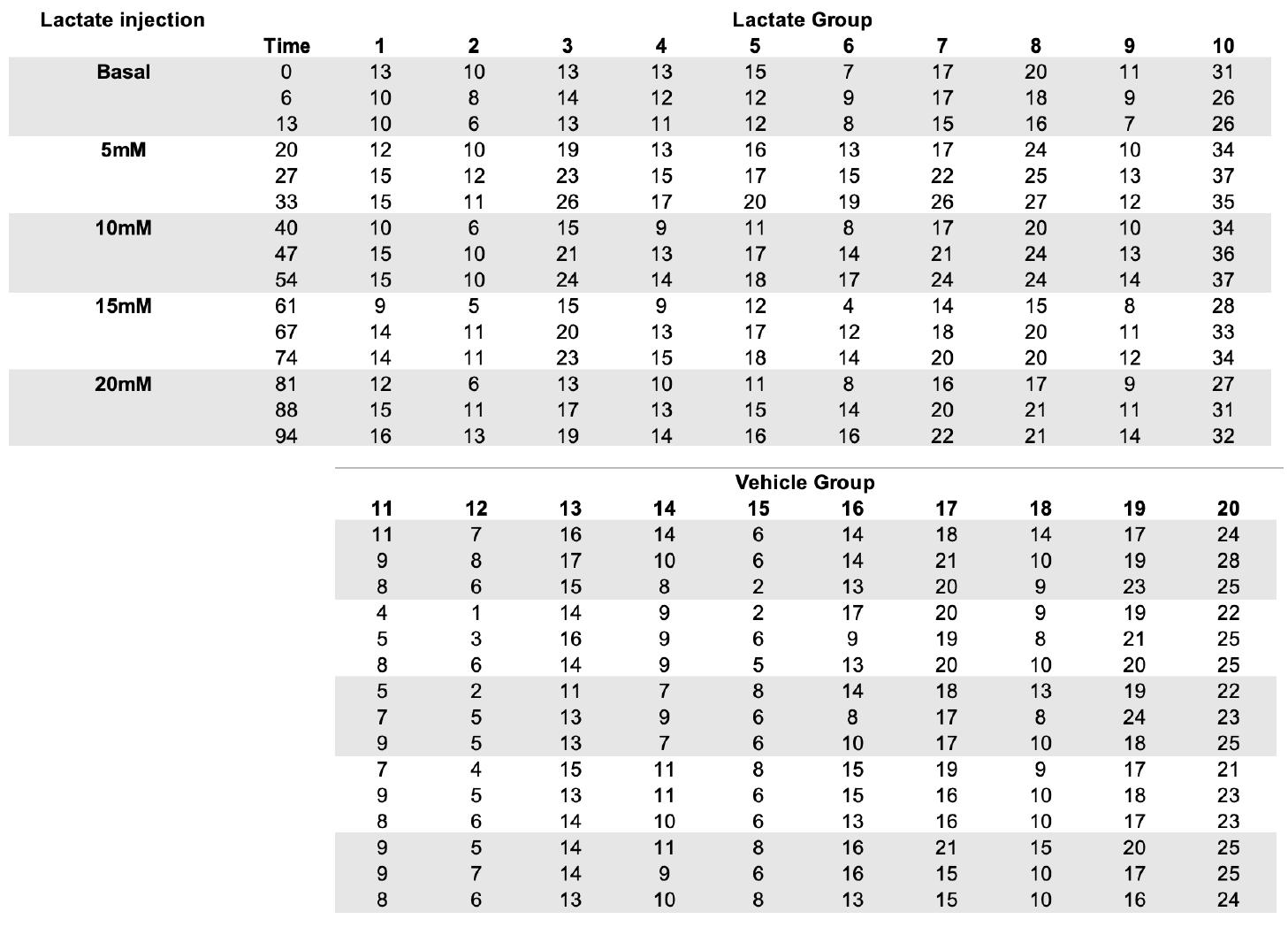
ECAR data The Journal of Science Extension Research – Vol. 2, 2023 education.nsw.edu.au 33
Bioaccumulation Of Microplastics And Their Respective Chemicals Within Seafood Of Different Trophic Levels: A Meta Study
 Flynn Croaker Coffs Harbour Senior College
The increasing amount of microplastics (MPs) in the ocean raises concerns regarding the bioaccumulation of harmful and toxic chemicals which build up in seafood species. This meta looked at current data and surveyed the available information to depict whether different trophic levels make sea creatures that are commonly eaten by humans more susceptible to MPs and their respective chemicals which cause bioaccumulation. The results showed that there are discrepancies in the amount of information available, however, there is a good amount of evidence supporting that lower trophic levels are more susceptible to MP consumption and the toxic chemicals that accumulate. There would need to be an increase in laboratory-based experiments on the topic to have certain results.
LITERATURE REVIEW
Microplastic Identification
Microplastics are microscopic pieces of plastic that are less than 5mm in diameter. These can be either primary or secondary pieces. Primary MPs are small particles created for commercial use, this also encompasses microfibers that have rubbed off clothing and other materials. Secondary MPs are plastic pieces that have broken down from a larger piece of plastic, this decomposing is caused by environmental factors, usually ocean waves and the sun’s radiation waves. Since these foods are small, they are quite frequently mistaken throughout the marine food chain as food. As these MPs break down further, they can give off toxic chemicals which can be harmful to these animals.
Seafood Identification
Any sea creature which is known to be eaten by any general population regardless of the circumstances e.g. a cultural food or a nation's traditional food.
Trophic Level Calculation (Diet Composition)
Trophic levels depend upon what a species eats. It can be obtained from
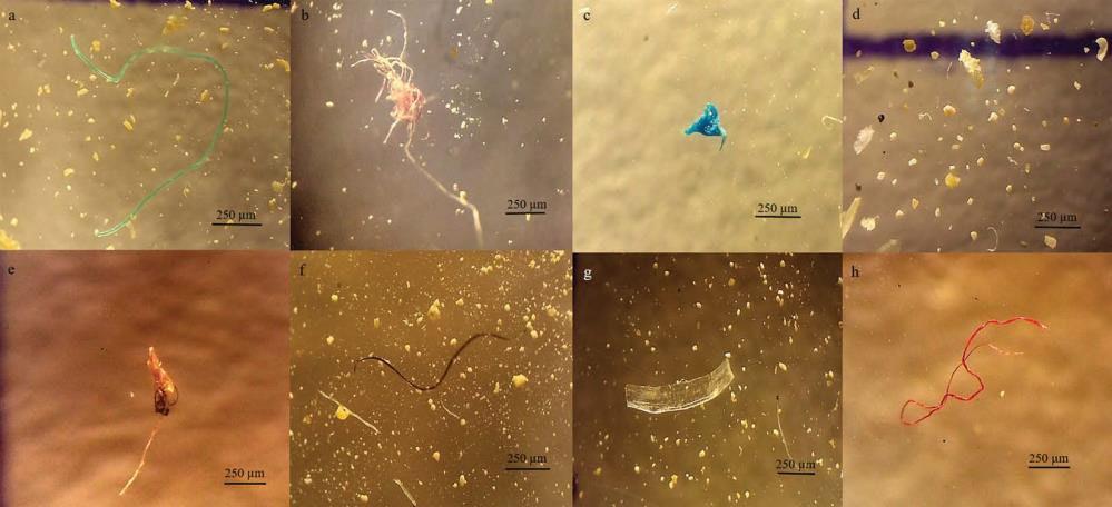
Figure 1. Some detected microplastics (MPs) in seafood species’ muscles from the Persian Gulf. The scale bar represents 250 μm. (Akhbarizadeh, Moore & Keshavarzi 2019)
The Journal of Science Extension Research – Vol. 2, 2023 education.nsw.edu.au 34
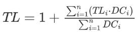
stable isotopes analyses, trophic ecosystem models, or stomach content analyses. As an example, a fish consuming 50% herbivorous-zooplankton (trophic level 2) and 50% zooplanktoneating fish (trophic level 3) would have a trophic level of 3.5. Trophic levels (TL) can be calculated from where n is the number of species or groups of species in the diet, DCi is the proportion of the diet consisting of species i, and TLi is the trophic level of species i. Thus, using dietary data, the trophic level of the predator is determined by adding 1.0 to the average trophic level of all the organisms that it eats. (Yodzi, Reichle & Trites 2017)
Trophic Transfer of Microplastics
The trophic magnification factor (TMF) was calculated mathematically based on the relationship between trophic level (TL) and the concentration of contaminants. TMF was calculated using the following equation:
TMF = eb
Where b is the slope of the equation below:
lnCbiota = a + (b x TL)
If TMF of a contaminant is below 1, the contaminant is not biomagnified (Won et al. 2018) and (Akhbarizadeh, Moore & Keshavarzi 2019)
QUESTION
Research question: Do MPs and their respective chemicals cause
bioaccumulation more within seafood of lower trophic levels?
HYPOTHESES
Alternative Hypothesis: Seafood species of lower trophic levels will be more susceptible to the bioaccumulation of MP chemicals.
Null hypothesis: Seafood species of higher trophic levels will be more susceptible to the bioaccumulation of MP chemicals.
METHOD
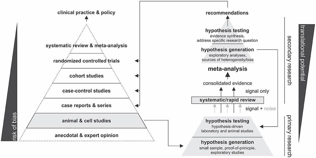
To present a meta-analysis and systematic review of all scientific literature globally, analysing the data on MP contaminants within specific aquatic species. This literature was screened through a rigorous framework [Fig 1]. A thorough search was conducted to find literature regarding the bioaccumulation of MPs within seafood species of different trophic levels. The exploration for literature was not limited to a specific search platform and was finalised in August 2022, covering the years 2012 to 2022. The search included the following terms: Microplastics, bioaccumulation, fish, effects, toxic and impacts. If they fit this model, the data was scrutinised and isolated, allowing the location of relevant information which was study specific. Meta-analysis then took place, and the amount of data would need to be sufficient to support the study. Further, they also had to meet a level of validity. This was calculated through their study level and risk of bias [Fig 2]. Any literature which did not sufficiently satisfy these requirements was not included. These sources had to also uphold a deeper level of conceptual conclusions and analysis within their results and have a clear,
The Journal of Science Extension Research – Vol. 2, 2023 education.nsw.edu.au 35
descriptive research method. Additional resources were acquired through the bibliographies from the literature that was going to be used. Once the relevant resources were acquired, the data was extracted and consolidated, this entailed extracting the relevant data to the specific research area and then making an assessment of the quality of the studies. This collected data was then evaluated to highlight the extent of between-study inconsistency (heterogeneity). Those results were pooled to calculate summary measures and the measure of effect, expanding the analysis on a macro study scale. These summaries created a general overall regression for the data, giving a trend in which the information was heading. These findings were then interpreted and provided recommendations within discussion for future works regarding the bioaccumulation of MPs within seafood species.
Figure 1.
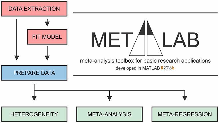
with graphical data extraction from study figures. Fit Model module applies MonteCarlo error propagation approach to fit complex datasets to model of interest. Prior to further analysis, reviewers have opportunity to manually curate and consolidate data from all sources. Prepare Data module imports datasets from a spreadsheet into MATLAB in a standardized format. Heterogeneity, Metaanalysis and Meta-regression modules facilitate meta-analytic synthesis of data. (Mikolajewicz 2019)
RESULTS
[Figure 1] suggests that there is a significant correlation between the
General framework of MetaLab. The Data Extraction module assists
Figure 2. Proposed Framework of the validity through a process of considering both risk of bias and level of research. (Mikolajewicz 2019)
The Journal of Science Extension Research – Vol. 2, 2023 education.nsw.edu.au 36
amount of microplastic intake that occurs as trophic levels change. This graph proposes that seafood of a higher trophic level will be subject to less microplastic intake, making them less susceptible to bioaccumulation. This may be because the higher a sea creature's trophic level, the less likely they are to be directly affected by the lower trophic level’s accidental consumption of MPs mistaking them for food. The Portunus armatus remains an outlier and this may be because of the foods in its diet which are mostly made up of smaller organisms which cannot accumulate a lot of MPs. This puts forward that this diet is a not particularly prevalent occurrence, some organisms throughout all trophic levels which are made an anomaly due to their diets. The results within the trophic magnification factor (TMF) calculation suppose that the contaminants were not biomagnified throughout the food web because the TMF was below 1, causing no development of bioaccumulation within the animals of higher trophic levels (TMF=0.72). This study put forward that biomagnification was not occurring in their studied organisms through their diet as the Biomagnification factor (BMF) < 1.
This data proposes that there are, on average, the most MPs within seafood from trophic levels 2-3 and 5. Level 1 is almost ruled out completely as it is composed of microorganisms that break down the food they consume, making them not as susceptible to bioaccumulation. There is a very significant difference between the results recorded in situ and in the laboratory. The lab has a much higher number of MPs per individual, this is most likely because of the controlled nature of the environment, allowing them to observe the changes in bioaccumulation of MPs, which again in [Fig 2. D] reaffirms that most MP bioaccumulation occurs within seafood around the trophic level of 2.5. Though in situ it is by chance whether species consume a higher number of MPs, however, it is clear to see a distinction between the means [Fig 3. a) and b)] across all the trophic levels, supporting the theory that around levels 2-3 and 5, more bioaccumulation takes place. This random intake in situ is the cause for so many outliers, all of which aren't able to be correlated according to their trophic level, and this randomness is controlled when in the lab, as the results prove there to be fewer outliers except for at trophic level 2, potentially because they are more susceptible to mistaking MPs for food based on their diet.
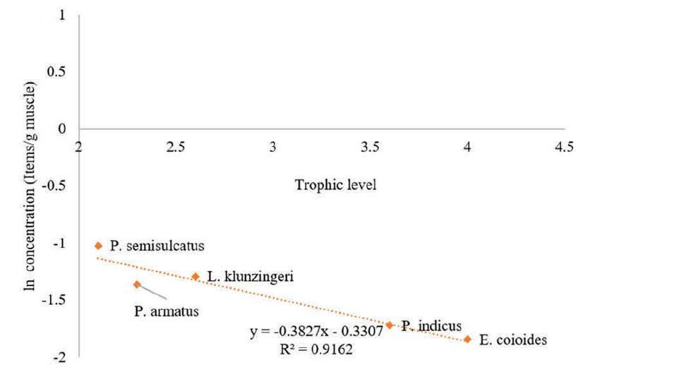 Figure 1. Relationship between MPs and trophic level of studied organisms from the Persian Gulf. (Akhbarizadeh, Moore & Keshavarzi 2019)
The Journal of Science Extension Research – Vol. 2, 2023 education.nsw.edu.au 37
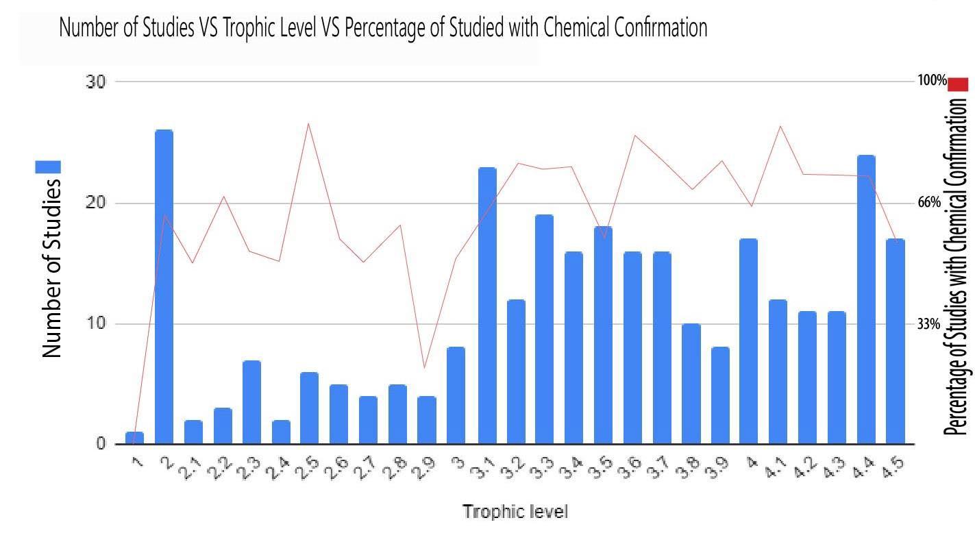
Upon looking at [figure 3] there’s an immediate realisation surrounding the lack of data from levels 2 to 3, even though there is still a large number of studies encountering MP chemical bioaccumulation. The significant difference between 2.8 and 2.9 is most likely due to the lack of results, therefore the data may not be accurate. There doesn’t at first appear to be a specific trend in the chemical confirmations, however, something to note is the spike
at trophic level 2.5, an area which has been of interest in other studies too, being the largest spike in MP intake, bioaccumulation and chemical accumulation as well. If the amount of study being done from 2-3, it would be assumed that there would be similar fluctuating results, however, there would most likely be a slightly lower average due to their trophic level being lower, meaning that they’re more likely to live a shorter life, not allowing for as much
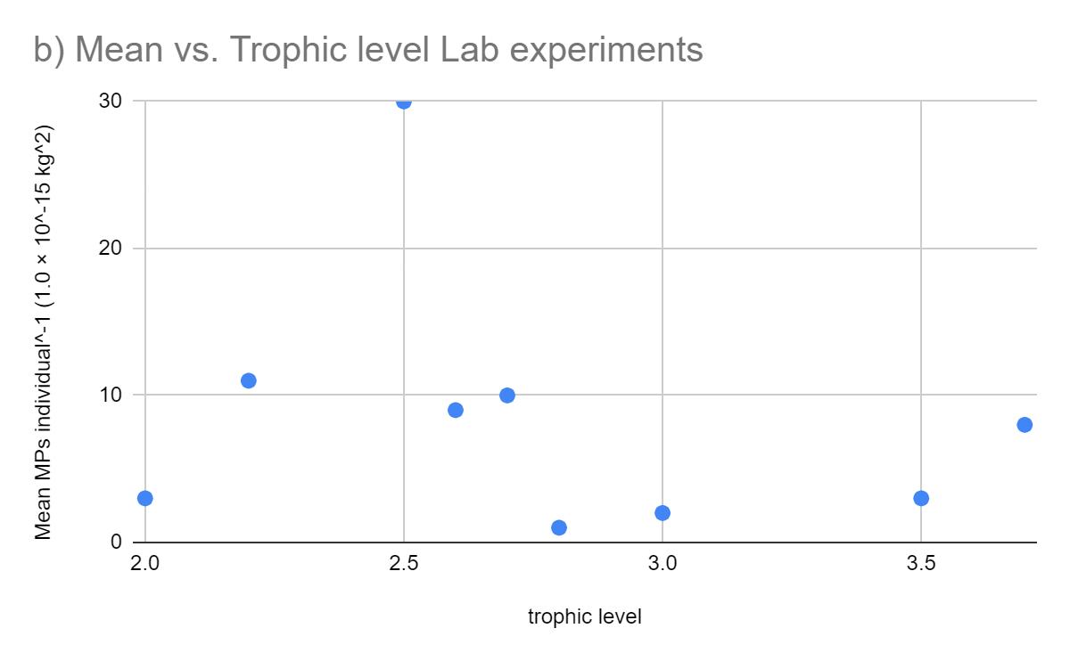
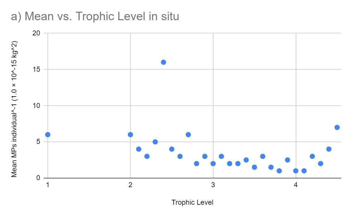 Figure 2. Body burden of bioaccumulated microplastics individual-1 estimated for different trophic levels, based on reports for marine species (a) collected in situ from levels 1 to 4.5 and (b)exposed in laboratory experiments from levels 2 to 3.7. Trophic levels have been grouped into to a single decimal place, e.g. level 4.2 includes 4.21 to 4.29. (Miller, Hamann & Kroon 2020)
The Journal of Science Extension Research – Vol. 2, 2023 education.nsw.edu.au 38
accumulation of toxic chemicals from MPs.
Within low abiotic concentrations, there is a constant downward trend, this infers that the higher the trophic level, the fewer MPs they have. As the simulation goes on, some sea creatures move up the levels system. This increase in the levels lowers the amount of bioaccumulation that takes place, again reaffirming the previous studies of which’s data has shown that there is a substantial increase in bioaccumulation/MP intake at around the level of 2.5. Something interesting about this data is that as time goes on, the trend steepens [fig 5 C-D] and then it flattens out with a lack of correlation, suggesting that in the end, all species will
bioaccumulate the same number of MPs over the long term. In the high abiotic simulation, this trend does not remain [fig. 6]. Proving that at the start of the simulation there was a much stronger correlation than in the longer term, which has no significant direction or correlation, appearing to be quite random. This ending in the data, though over a longer time, with no clear direction in the data, appearing to be flat also suggests that over the long term, the species will have roughly the same amount of MP bioaccumulation. The randomness of this in situ study suggests that the correlation could be stronger if given the right data set.
Fig 3. Frequency of microplastic (MP) chemicals confirmed in comparison to the number of studies done. Reporting on studies with marine species collected in situ. Data has been organised by trophic level, which are grouped into to a single decimal place, i.e. level 4.2 includes 4.21 to 4.29. (Miller, Hamann & Kroon 2020)
The Journal of Science Extension Research – Vol. 2, 2023 education.nsw.edu.au 39
Figure 5. Projections of the apparent trophic magnification factor (TMF) as a function of predicted concentration of microplastics (MPs) versus trophic level (TL) in the cetaceans’ food web of the Northeastern Pacific for simulations under a scenario of low abiotic concentrations (scenario 1: seawater = [0.003 particles/L]; and sediment = [0.266 g/kg dw] at: (A) 5 days (lack of significant relationship); (B) 10 days (regression line indicates a strong negative, significant relationship); (C) 25 days (regression line indicates a moderate and negative, significant relationship); (D) 50 days (regression line indicates a weak and negative, significant relationship); (E) 100 days (lack of significant relationship); (F) 365 days or 1 year (lack of significant relationship); (G) 3650 days or 10 year (lack of significant relationship); and (H) 36500 days or 100 year (the dotted line indicates the slope direction and a negative positive trend, but lack of a significant relationship). (Alava 2020)
The Journal of Science Extension Research – Vol. 2, 2023 education.nsw.edu.au 40
Figure
factor (TMF) as a function of predicted concentration of microplastics (MPs) versus trophic levels (TL) in the cetaceans’ food web of the Northeastern Pacific for simulations under a scenario of high abiotic concentrations (scenario 3: seawater = [0.04 g/L]; and, sediment = [111 g/kg dw] at: (A) 5 days (the regression shows lack of significant relationship); (B) 10 days (regression line indicates a negative, significant relationship); (C) 25 days (dotted line indicates a negative trend but not a significant relationship; (D) 50 days (dotted line indicates a negative trend, but lack of significant relationship); (E) 100 days (dotted line indicates a negative trend, but lack of significant relationship); (F) 365 days or 1 year (lack of significant relationship); (G) 3650 days or 10 years (lack of significant relationship); and (H) 36500 days or 100 year (lack of significant relationship). (Alava 2020)
The Journal of Science Extension Research – Vol. 2, 2023 education.nsw.edu.au 41
6. Projections of the apparent trophic magnification
This logarithmic data set provides insight into the nature of when the most MPs are consumed within different seafood species. Certain species such as the gonatid squid increase their intake of MPs as they get older; in comparison to a Dungeness crab which is very limited in its increase of accumulated MPs over time, has a plateau-like statistic from around 120 days. This may suggest that the Dungeness crab learns how to tell the difference between MPs and real food early on in their lifespan. This is
surprising as they sit around a 2.7 trophic level, placing them near the usually spiking 2.5 trophic level. There isn’t a specific weight of MPs that all species meet at the end of the simulation as potentially suggested in [Figs 5 and 6] however, this graph suggests that there is quite a widespread in the closing MPs weight. Around 30 days it is clear to see that there is a very similar and strong correlation between all the seafood species and their MP weight, all sitting around 0.005 g/kg.
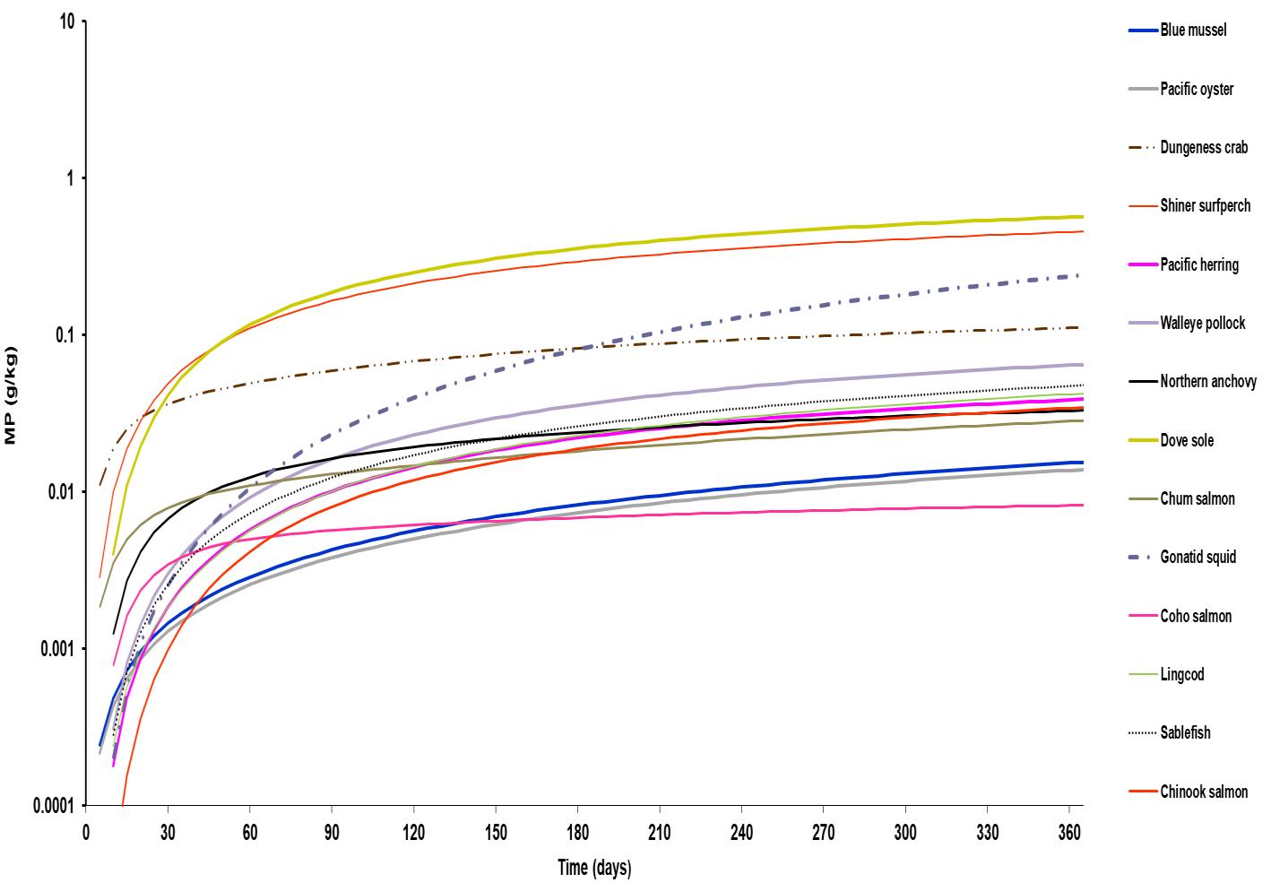
The Journal of Science Extension Research – Vol. 2, 2023 education.nsw.edu.au 42
Figure 7. Simulation presenting the projections of microplastics (MPs) bioaccumulation in seafood organisms derived from Alava's 2020 Mammalian Foodweb model simulation of projected microplastic bioaccumulation.
DISCUSSION
The data ultimately differs quite a lot between studies. This is because of the randomness within situ and the lack of data conducted within laboratories. There are studies that both confirm that more bioaccumulation takes place in levels 2-3, and in converse, there is one study that supports there being more accumulation of MPs within levels 3-4.5; This one study also explores the number of papers that have been done on the different trophic levels and it highlights a discrepant number of studies looking at lower levels, causing their data on the percentage of chemical confirmations to be potentially inaccurate. In summary, the data studied indicates that the seafood species which are around a 2.5 trophic level are the most susceptible to MP accumulation, however, there isn’t enough data in a controlled environment to be certain.
This supports the hypothesis given that the study suggests that fish of lower trophic levels will be more susceptible to the bioaccumulation of MP chemicals. These results suggest that if humans want to take the utmost measures to avoid MP consumption, they should avoid filter feeders (muscles, oysters, scallops etc.), deposit feeders (bass, eels, crabs etc.) and grazers (lobsters, shrimp etc.). The limitations of study are around the lack of research done in specific areas. These areas include lower trophic levels lack of studies done, and a lack of studies done in controlled environments such as labs to eliminate the randomness of data which can give clearer and more concise results, allowing for more accuracy and reliability. For further study, there would need to be a deeper understanding of the nature of MP bioaccumulation within all trophic levels, more studies would need
to be done in a laboratory setting that has more controlled variables. This is the future direction to further this area of research because the number of MPs the species are being exposed to can be limited by the people conducting the research, in comparison to in situ which varies depending on where the species are. However, the effects of doing a study in a lab could affect their eating habits and thus change the outcome of the final data, if this was the case there would just need to be a filling of the data done on lower trophic level seafood species in situ. This study could be implicated to give a deeper insight into the seafood which is the healthiest to eat regarding a lack of MP chemicals and MPs themselves, proving from this research to be food from higher trophic levels as they have appeared to have less MP bioaccumulation.
This report is an important step as it not only highlights the conclusions that can be drawn from existing studies but also proposes where there is a lack of data that can help further develop this area of study. The studies done were majorly targeting marine organisms rather than species that humans eat, meaning their research may have missed more in-depth seafood-specific data as it wasn’t what they were looking for. There is also the limitation that some of the figures used are based on simulations built upon calculations rather than actual real-world data. There is a seemingly larger focus on the biomagnification of MPs within food chains within marine ecosystems rather than bioaccumulation. This data could potentially be used and manipulated to draw further conclusions regarding bioaccumulation rather than biomagnification. A lack of correlation in some results is most likely due to the
The Journal of Science Extension Research – Vol. 2, 2023 education.nsw.edu.au 43
random nature of in situ environments, which may by chance show a lack of correlation between MPs and trophic levels, or in other studies, it may demonstrate a strong correlation, neither would be “wrong” however, this means a vast number of studies are needed to be done to average the data and gain a deeper analysis of the whole study area. This is why a suggested laboratory test would be more efficient as it can collect more specific results which aren’t limited to chance. This study can not only enable people to be aware of the seafood which is the least likely to have MPs, but it can also allow companies to target certain fish markets which are less susceptible to MP bioaccumulation, making their products more appealable.
CONCLUSION
The findings suggest that overall, there is a spike in MP bioaccumulation at trophic level 2.5. Generally, there is a higher number of MP intake from levels 2-3, however, due to the randomness of the in-situ setting, it is a lot harder to measure because of a lack of controllable variables in terms of how many MPs are introduced to different species. This information demonstrates an acceptance of the alternative hypothesis: Seafood species of lower trophic levels will be more susceptible to the bioaccumulation of MP chemicals. A study evaluating the amount of data there already is surrounding the MP consumption regarding the percentage of chemical confirmations within the species demonstrated that there was a significant discrepancy between the amount of research on MP consumption for seafood species in trophic levels 2-2.9, but there was a comfortable amount of study on levels 34.5. This posed the question of whether
the data and analysis were accurate, however, this is hard to judge as it is in a random environment rather than in a laboratory which would have a significant increase in the variables which could be controlled. In situ environments provide a lot less explainable results than if they were to be tested in laboratories, as the experiment conductor can target variables and isolate causes for different effects, however, in situ it could be one of many different unknown factors. Ultimately, there would need to be a lot more research in both situ and laboratories targeting specifically the different trophic levels, not leaving any discrepancies in what levels are tested, and targeting seafood species rather than general marine organisms, as it allows a further development of understanding which can be implemented to improve human health and quality of life.
ACKNOWLEDGMENTS
The author would like to acknowledge and thank all the sources which have contributed to the final conclusions of this study.
REFERENCES
1. Akhbarizadeh, R, Dobaradaran, S, Nabipour, I, Tajbakhsh, S, Darabi, AH & Spitz, J2020, ‘Abundance, composition, and potential intake of microplastics in canned fish’, Marine Pollution Bulletin, vol. 160, p. 111633.
2. Akhbarizadeh, R, Moore, F & Keshavarzi, B 2019, ‘Investigating microplastics bioaccumulation and biomagnification in seafood from the Persian Gulf: a threat to human health?’, Food Additives & Contaminants: Part A, vol. 36, no. 11, pp. 1696–1708.
The Journal of Science Extension Research – Vol. 2, 2023 education.nsw.edu.au 44
3. Alava, JJ 2020, ‘Modeling the Bioaccumulation and Biomagnification Potential of Microplastics in a Cetacean Foodweb of the Northeastern Pacific: a Prospective Tool to Assess the Risk Exposure to Plastic Particles’, Frontiers in Marine Science, vol. 7.
4. Andreas, Hadibarata, T & Sathishkumar, P 2021, ‘Microplastic contamination in the Skipjack Tuna (Euthynnus affinis) collected from Southern Coast of Java, Indonesia’, Chemosphere, vol. 276, p. 130185.
5. Haidich, AB 2010, ‘Meta-analysis in Medical Research’, Hippokratia, vol. 14, LITHOGRAPHIA Antoniadis I.Psarras Th. G.P., no. Suppl 1, pp. 29–37.
6. Hansen, C, Steinmetz, H & Block, J 2021, ‘How to conduct a metaanalysis in eight steps: a practical guide’, Management Review Quarterly.
7. Hussien, NA 2021, ‘Investigating microplastics and potentially toxic elements contamination in canned Tuna, Salmon, and Sardine fishes from Taif markets, KSA’, Open Life Sciences, vol. 16, no. 1, pp. 827–837.
8. Kim, J-H, Yu, Y-B & Choi, J-H 2021, ‘Toxic effects on bioaccumulation, hematological parameters, oxidative stress, immune responses and neurotoxicity in fish exposed to microplastics: A review’, Journal of Hazardous Materials, vol. 413, p. 125423.
9. Mikolajewicz, N 2019, ‘Meta-Analytic Methodology for Basic Research: A Practical Guide’, Frontiers in Physiology, vol. 10, no. 1.
10. Miller, ME, Hamann, M & Kroon, FJ 2020, ‘Bioaccumulation and biomagnification of microplastics in marine organisms: A review and meta-analysis of current data’, in A Mukherjee (ed.), PLOS ONE, vol. 15, no. 10, p. e0240792.
11. Rios-Fuster, B, Alomar, C, Viñas, L, Campillo, JA, Pérez-Fernández, B, Álvarez, E, Compa, M & Deudero, S 2021, ‘Organochlorine pesticides (OCPs) and polychlorinated biphenyls (PCBs) occurrence in Sparus aurata exposed to microplastic enriched diets in aquaculture facilities’, Marine Pollution Bulletin, vol. 173, p. 113030, viewed 10 September 2022
12. Schäfer, S 2015, ‘Bioaccumulation in aquatic systems: methodological approaches, monitoring and assessment’, Environmental Sciences Europe, vol. 27, no. 1.
13. Stanley, M 2022, Microplastics | National Geographic Society, education.nationalgeographic.org, National Geographic Society.
14. Won, E-J, Choi, B, Hong, S, Khim, JS & Shin, K-H 2018, ‘Importance of accurate trophic level determination by nitrogen isotope of amino acids for trophic magnification studies: A review’, Environmental Pollution, vol. 238, pp. 677–690.
15. 15. Yodzi, P, Reichle, DE & Trites, AW 2017, Trophic Level - an overview | ScienceDirect Topics, Sciencedirect.com.
APPENDIX
https://docs.google.com/spreadsheets/d/1 FdGtaQpN8HiI75qMaMzWecu7l1cj1oudy 5ToyJWvLDQ/edit?usp=sharing
The Journal of Science Extension Research – Vol. 2, 2023 education.nsw.edu.au 45
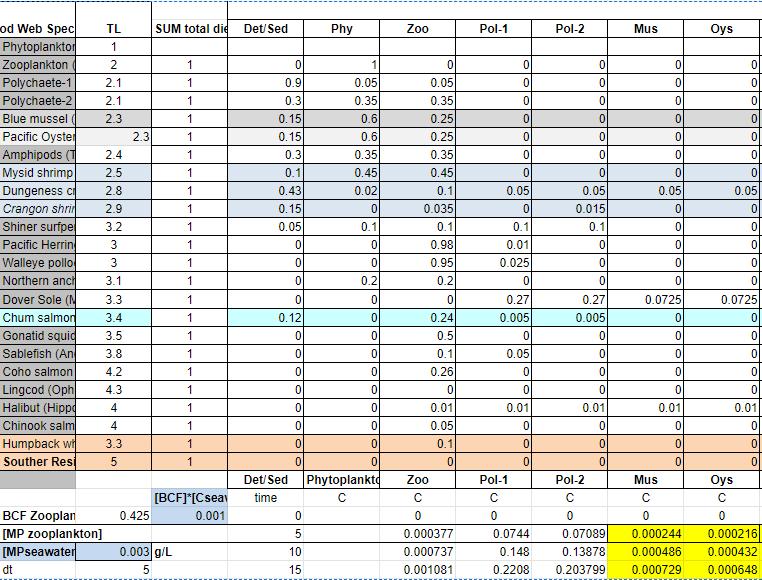
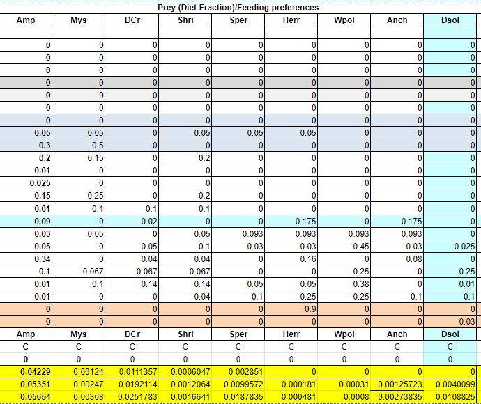
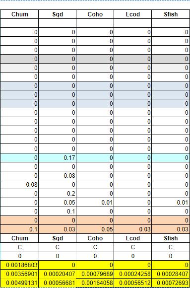
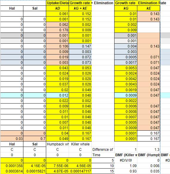
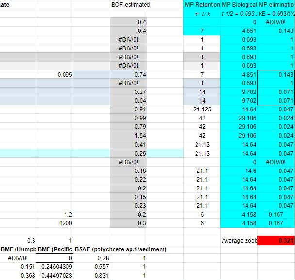
The Journal of Science Extension Research – Vol. 2, 2023 education.nsw.edu.au 46

The Journal of Science Extension Research – Vol. 2, 2023 education.nsw.edu.au 47
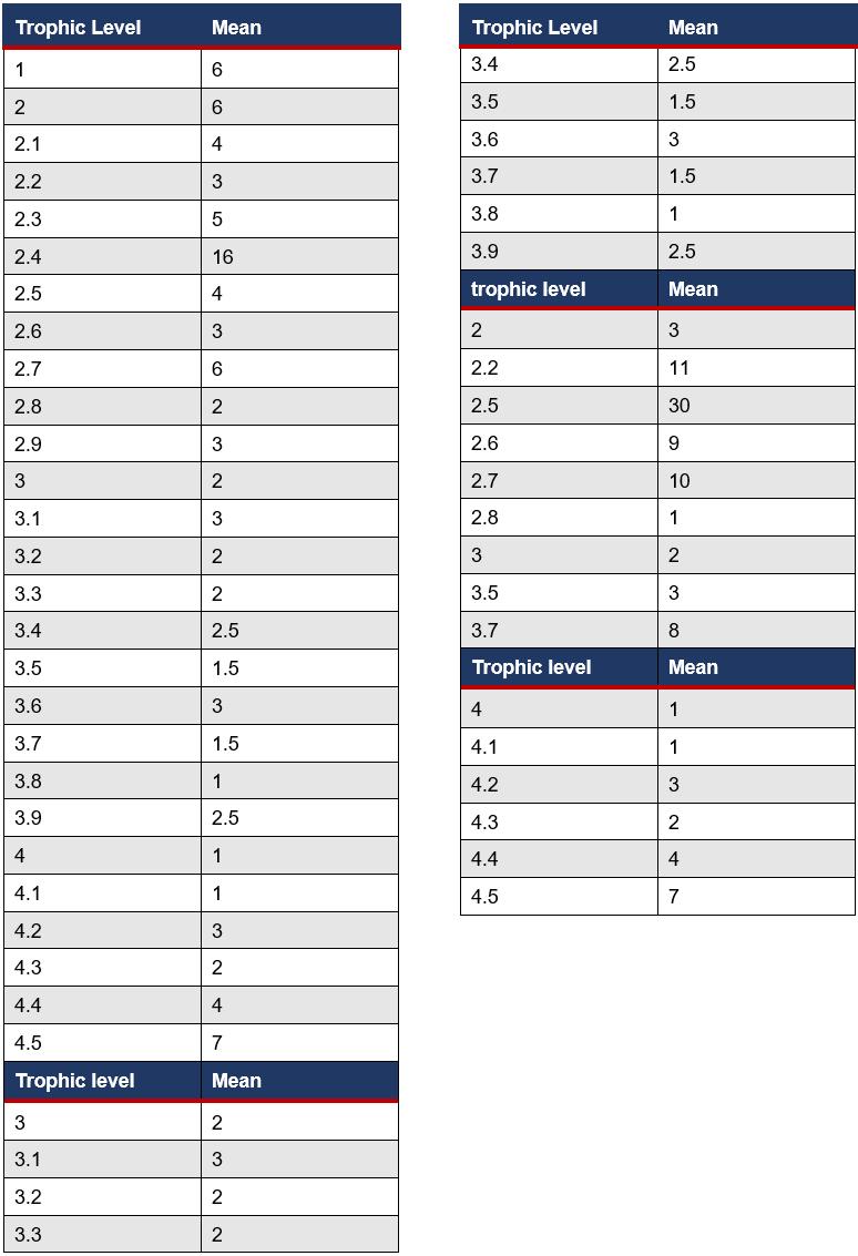
The Journal of Science Extension Research – Vol. 2, 2023 education.nsw.edu.au 48
Testing the effect of environmental conditions on photosynthesis production
Lena Dayil Lurnea High School
Photosynthesis is important as it sustains life by releasing oxygen into the atmosphere and provides energy for food chains which is the reason behind the conduction of this experiment. The investigation focuses on the environmental factors of temperature, sunlight vs shade and the colour of the plants (chlorophyll concentration) and their effect on the rate of photosynthesis when tested through the floating leaf disk assay. The plants were exposed to different environmental conditions in order to obtain accurate and precise results. The results were analysed through using mean, standard deviation and also through the statistical analysis. Main results included that higher temperatures allow for an increased rate of photosynthesis, better sunlight/light intensity also increases photosynthesis rate, while the colour of the plant needs to be a darker green as it has a higher chlorophyll concentration which increases photosynthetic rate. Overall, It allows individuals to know under which environmental conditions plants grow best in order to have a higher photosynthesis rate, however for the results to be comprehensive more environmental results need to be tested. Further investigations need to be carried out in order to confirm the accuracy, reliability and validity of the results.
Literature review
All living organisms need oxygen to grow and reproduce. Plants do not consume food like humans and animals, instead they convert light energy, water and carbon dioxide into oxygen and sugar. Plants make their own energy through a process called photosynthesis. This is important in agriculture as it provides nutrients for the crop and in photosynthesis, plants constantly absorb and release gases in a way which creates sugar for food. Plants convert light energy, water, and carbon dioxide into oxygen and sugar. They can then use the sugar as an energy source to fuel their growth.
Photosynthesis provides energy that drives all the plants metabolic functions, it
is the main source of food on earth which provides us with fibre, medicine and fuel, it releases oxygen which is the most important element for the survival of all life. It is also the most significant part of the food chain as many animals have plants as their only food source.
Photosynthesis takes place in the chloroplasts within the plant's cells. The chloroplasts contain special pigments that react to light. Chlorophyll is one of the pigments that can absorb light in the blue and red spectrum from the visible light spectrum. Chlorophyll does not absorb light in the green spectrum of light but reflects it instead. This is why leaves with chlorophyll usually appear green. During the first part of photosynthesis the lightdependent reaction chlorophyll and other pigments harness the light energy to produce NADPH (nicotinamide adenine
The Journal of Science Extension Research – Vol. 2, 2023 education.nsw.edu.au 49
dinucleotide phosphate) and ATP, (triphosphate) which are two types of energy-carrier molecules. At the same time, water is split into oxygen (O2) and protons (H+). The next stage is lightindependent and is often referred to as the dark reaction. In this step, the two energy-carrier molecules, NADPH and ATP, are utilised in a series of chemical reactions called the Calvin cycle. In the Calvin cycle, the plants take carbon dioxide (CO2) from the air and use it to ultimately make sugars such as glucose or sucrose. These sugars can be stored for later use by the plant as an energy source to fuel its metabolism and growth.
Photosynthesis is beneficial in aquaculture as it supplies fish ponds with oxygen, removes carbon dioxide and removes wastes such as nitrates, ammonia and urea. Photosynthesis is slower underwater as it is difficult for the light to reach underneath the water in places such as oceans. The most
important factor of photosynthesis in agriculture is food production. The world’s demand for food is constantly increasing, this is why it is important for scientists and farmers to understand photosynthesis and explore the potential improvements of photosynthesis that can cause faster plant growth. If farmers find a way to increase the rate of photosynthesis then that will also increase the yield of the crop which is why the rate of photosynthesis and this topic are highly significant.
In the near future the demand for food will be enormous. The rising human population and the changing patterns in land use mean that the world's food production rates will need to be increased by at least 50% by 2050. Most of this extra demand comes from developing countries and grain demand is also expected to increase highly over the next two decades.
The Journal of Science Extension Research – Vol. 2, 2023 education.nsw.edu.au 50
Figure 1: graph representing the increase in food demand within a range of countries
Light intensity
Light intensity impacts the rate of photosynthesis as higher light intensity means more light called "photons" are available to hit the leaves of the plant. The rate of photosynthesis can increase when there is more light available as it will allow the plant to drive all the reactions that are necessary for photosynthesis to occur. Too much light for a plant can also be negative causing dryness meaning that light intensity has a limit.
Literature data
2021. [online] Available at: <http://www.esalq.usp.br/lepse/imgs/cont eudo_thumb/How- does-the-level-of-lightaffect-the-rate-of-photosynthesis.pd>
[Accessed 8 December 2021].
Explains the environmental condition of light intensity and how it is related to the rate of photosynthesis, (the improvements in the conversion of light energy has been the central part of a crop's improvement.)
Temperature
The chemical reactions which allow photosynthesis to occur, and the combining of carbon dioxide and water for the production of glucose are all controlled by enzymes. The rate of photosynthesis is affected by temperature.
Low temperatures cause the rate of photosynthesis to be decreased and leads to a decrease in glucose production causing stunted growth in the plants. Medium temperatures allows the enzymes to work at optimum levels
leading to an increase in photosynthesis rates while High temperatures causes the enzymes to denature, not work efficiently and makes them lose their shape leading to a decline in the photosynthesis rate.
Scientific research question
‘Which type of environmental factors (sunlight vs shade (light intensity), temperature and colour of plant) affect the rate of photosynthesis in different plant seedlings (Chilli, rose apple plant and parsley) when tested through the floating leaf disk assay.’
Scientific hypothesis
‘Without optimal amounts of sunlight, appropriate lighting and optimal temperature, a plant's photosynthesis rate will decrease.’
Methodology
Choosing and growing appropriate plants for investigation.
The plant that was chosen includes chilli which was tested through temperature, light intensity and the colour of the plant/chlorophyll concentration. Species were grown in different conditions over a period of 9 weeks in spring 2022 in sample groups of 10 seedlings per condition. The floating leaf disk assay is found on the sciencebuddies website, (https://www.sciencebuddies.org/) which was reconstructed and adapted in order to create a new experiment. For detailed methods, visit the appendixes.
Floating leaf disk assay
The floating leaf disk assay utilises the rate at which oxygen is produced or consumed as a measure of the processes of photosynthesis. Disks are punched
The Journal of Science Extension Research – Vol. 2, 2023 education.nsw.edu.au 51
from leaf tissue and a vacuum is used to replace air in the spongy mesophyll with liquid, making the disks sink. As photosynthesis takes place in light, oxygen is produced. The accumulating gas makes the disks buoyant and they float. The rate of photosynthesis in the leaf disks is calculated after determining the time required for submerged leaf disks to float.

2. Leaf assay picture Analysis of results
The results were analysed using both descriptive and inferential, using appropriate statistical methods (mean, standard deviation and student's T test) using Microsoft Excel 365.
The results have been analysed by comparing them to the results of other individual’s experiments which have similar qualities and features to this investigation and also using appropriate statistical tests to determine the significance of the results. Figure 2 provides an example of results done by another individual who did a similar experiment to this by using the floating leaf disk assay which is highly useful for the data analysis. A good way to collect data is to count the number of floating disks at the end of a fixed time interval; for example, after every minute until all disks are floating. The time required for 50% of the leaves to float represents the Effective Time (ET50). ET50 can be determined by graphing the number of disks floating over time, as shown in Figure 2. An ET50 of 11.5 minutes, for example, as shown in Figure 2, would mean that after 11.5 minutes, 50% of the leaves (5 out of the 10) floated on top of the baking soda solution. In the context of oxygen production, you could also say that an ET50 value of 11.5 minutes means that it took 11.5 minutes to produce enough oxygen to make 50% of the leaf disks float.
Figure
The Journal of Science Extension Research – Vol. 2, 2023 education.nsw.edu.au 52
Results


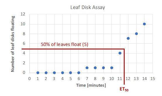 Figure 3: Example results for a different floating leaf disk assay. The graph shows the time on the x-axis and the number of floating leaves on the y-axis. The Effective Time (ET50) represents the time required for 50% of the leaves to float. By extrapolating from the graph, the 50% floating point in this graph is about 11.5 min.
Figure 4: Experimental setup for the sunlight vs shade experiment.
Figure 3: Example results for a different floating leaf disk assay. The graph shows the time on the x-axis and the number of floating leaves on the y-axis. The Effective Time (ET50) represents the time required for 50% of the leaves to float. By extrapolating from the graph, the 50% floating point in this graph is about 11.5 min.
Figure 4: Experimental setup for the sunlight vs shade experiment.
The Journal of Science Extension Research – Vol. 2, 2023 education.nsw.edu.au 53
Figure 5: experimental setup for the first experiment (temperatures of hot, cold and room.)
Figure
9 floating leaf disks are visible/can be counted in this image in the hot water temperature of (37 degrees) which both reduces bias and increases accuracy of results.
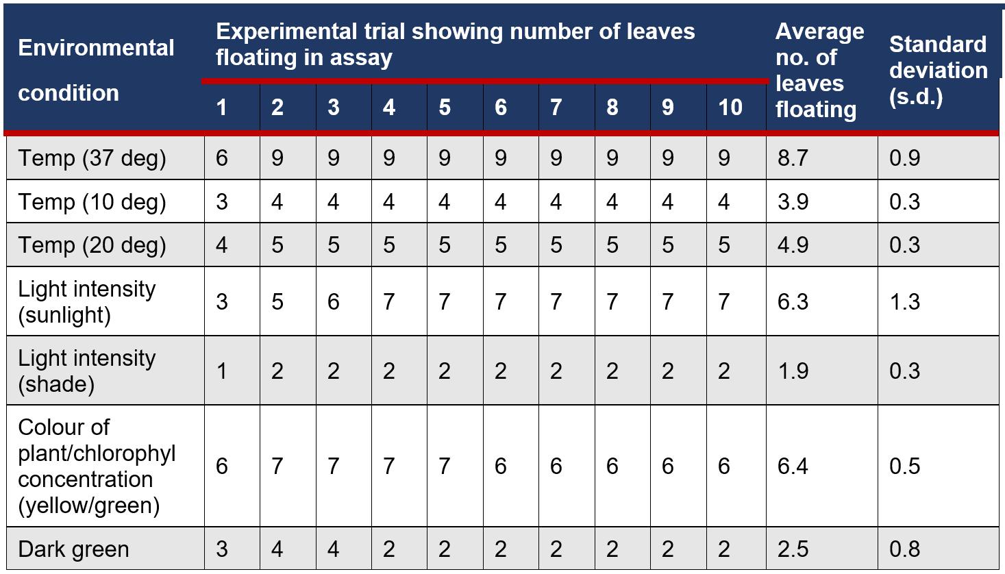

Treatment 1 (left) is hot water (37 deg), Treatment 2 (middle) is cold water (10 deg) and treatment 3 (right) is room temperature (20 deg.) Through analysis of this graph, it is clearly evident that the higher the temperature goes, the higher the rate of photosynthesis is.
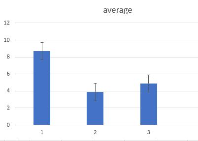 6: The
Figure 7: Graph illustrating all the experimental results (trials for each environmental condition), including the mean/average and standard deviation.
6: The
Figure 7: Graph illustrating all the experimental results (trials for each environmental condition), including the mean/average and standard deviation.
The Journal of Science Extension Research – Vol. 2, 2023 education.nsw.edu.au 54
Figure 8:
evident that plants which are exposed to sunlight produce an increased photosynthesis rate.
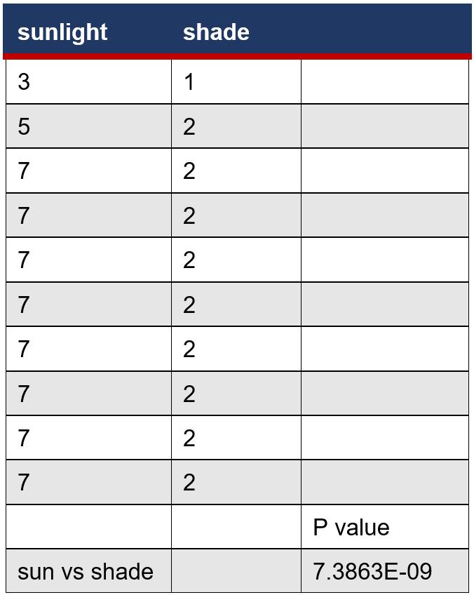
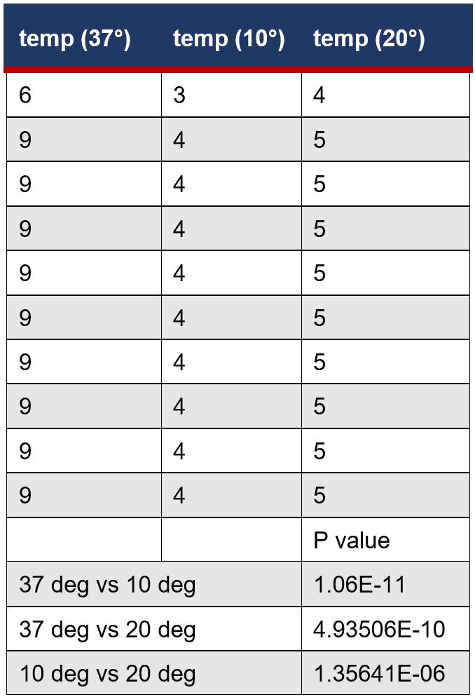
the colour of the plant/chlorophyll concentration and the role it plays in photosynthesis production. The lighter (orange/yellow plant) on the right of the graph highlights decreased photosynthesis rate, while the darker green plant (which has the higher chlorophyll concentration) on the left of the graph, has an increased and higher photosynthesis rate production than the lighter coloured plants.

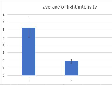 Figure 9: Treatment 1 (left) illustrates the results for sunlight exposure of the plant, while treatment 2 (right) exposes the results for the plant which was in the shade. Through analysing this graph, it is clearly
Figure 10: Demonstrates
Figure 11: Statistical test of the temperatures
Figure 9: Treatment 1 (left) illustrates the results for sunlight exposure of the plant, while treatment 2 (right) exposes the results for the plant which was in the shade. Through analysing this graph, it is clearly
Figure 10: Demonstrates
Figure 11: Statistical test of the temperatures
The Journal of Science Extension Research – Vol. 2, 2023 education.nsw.edu.au 55
Figure 12: Statistical test of results from sun vs shade
Discussion
Through analysing and interpreting the results, it can be seen that environmental factors such as temperature, light intensity and the colour of the plant have an effect on the rate of photosynthesis. Temperature has an effect on the rate of photosynthesis as higher temperatures (hotter) increase photosynthesis, due to the fact that photosynthesis is a chemical reaction which is accelerated with temperature, but at extremely high temperatures, the enzymes that carry out photosynthesis can lose their shape and functionality, and the photosynthetic rate declines rapidly. The graph within figure 8 highlights this as higher temperatures lead to an increased photosynthesis production. This is demonstrated within the results as in the beaker which
contained the hot water (37 degrees celsius) 9 of the floating leaf disks floated to the top, while in the beaker that contained cold water (10 degrees) only 4 had risen to the top. Enzymes are protein molecules used by living organisms to carry out biochemical reactions. The proteins are folded into a particular shape, and this allows them to bind efficiently.
At low/cold temperatures (10 degrees) photosynthesis rate declines, this is illustrated in figure 8 as the cold temperature water had the least amount of floating leaf disk assays floating to the top of the beaker (only 4), the enzymes that carry out photosynthesis did not work efficiently, and this decreased the photosynthetic rate. This leads to a decrease in glucose production and will result in stunted growth within the plant. At medium/room temperatures, (20 degrees) the photosynthetic enzymes work at their optimum levels, so photosynthesis rates are generally high. Within the results, the beaker which contained room/optimal temperature, 5 of the floating leaf disk assays had risen to the top. Highlighting the effect that different temperatures have on photosynthesis rate within plants and that higher temperatures lead to a higher photosynthesis rate.
Light intensity is one of the important factors which affect the rate of photosynthesis. Light intensity directly affects the light-dependent reaction in photosynthesis and indirectly affects the light-independent reaction. Very high light intensities may slow the rate of photosynthesis due to the bleaching of chlorophyll. However, plants exposed to such conditions usually have protective features such as thick, waxy cuticles and
 Figure 13: Statistical test of the colour of plant/chlorophyll concentration
The Journal of Science Extension Research – Vol. 2, 2023 education.nsw.edu.au 56
hairy leaves. Increasing the light intensity increases the rate of photosynthesis, until another factor (limiting factor) becomes in short supply.
This is expressed within the results as in figure 9, the beaker with the plant that was exposed to sunlight had more floating leaf disks (7) rising to the top of the beaker, while treatment 2 which involved the plant being exposed to more shade had less floating leaf disks floating (only 2). This illustrates the powerful effect that higher light intensity has on increasing the rate of photosynthesis as it is clearly evident that plants which are exposed to sunlight produce an increased photosynthesis rate.
If a plant is a darker green, then it should photosynthesize faster as the plant contains more chloroplasts and thus has more chlorophyll (a pigment) which is one of the most important components for photosynthesis to occur. Chlorophyll absorbs the light energy required to convert carbon dioxide and water into glucose. Chlorophyll is green meaning that it absorbs the red and blue parts of the electromagnetic spectrum and reflects the green part of the spectrum. Leaves with more chlorophyll are better able to absorb the light required for photosynthesis. This is reflected within my results as the graph within figure 10 illustrates that the beaker which contained the dark green plant (which has a higher chlorophyll concentration) allowed more photosynthesis to be produced due to more floating leaf disk assays rising to the top (6-7) while the beaker which contained the lighter coloured part of the plant/leaf (yellow/orange) had less floating leaf disk assays (2) at the end of the trials/10 minutes as shown in figure 10. This
demonstrates the effect that chlorophyll has on photosynthesis in increasing it drastically.
Some limitations involved within this experiment include the temperature which could not be kept at a constant throughout the experiment. Experimental results and design need to be further investigated in order to further improve the investigation. Systematic uncertainties/errors and bias are those that occur due to faults in the measuring instrument or in the techniques used within the experiment. The accuracy of measurements subject to systematic errors cannot be improved by repeating those measurements. Systematic errors can be difficult to detect but once they are detected, they can be reduced by refining the methods and techniques. Systematic errors are deviations from the true value by a constant amount and they affect the accuracy. A systematic uncertainty within the experiment is the timer which was used to time how long it takes for the floating leaf disk assays to float to the top of the beaker, this is a uncertainty as it is difficult to start and stop the watch at the exact same points.
Within the investigation, bias is very limited as plants have been selected randomly. The experiment is reliable as there are a large number of trials (10). Repeating the experiment or testing a certain factor multiple times in order to make sure the results are similar is highly important within scientific investigations. The trials involved observing how many floating leaf disks floated to the top of the beaker at the end of each minute, until the time reached 10 minutes. Validity is also important as it determines whether the results/experiment answers the research question. The experiment
The Journal of Science Extension Research – Vol. 2, 2023 education.nsw.edu.au 57
contains validity as it tests the rate of photosynthesis under different environmental conditions through utilising the floating leaf disk assay. The experiment is also accurate as it involved proper planning of the equipment and materials used in the experiment. Mean and standard deviation are also methods used to calculate the results which increase the accuracy.
Qualitative data which was collected increases the validity of this investigation. Photographs were taken during the conduction of the experiment. Figure 4 and 5 provides evidence on how the experiment was set up, and figure 6 illustrates the 9 floating leaf disks which are floating at the top of the beaker which can be clearly seen and counted from the image. This was the hot temperature water of 37 degrees which had the most leaf disks floating to the top.
The statistical test performed was two tailed T test with equal variants in excel (tail=2) and (type=2). When the temperature of 37 degrees was compared with the temperature of 10 degrees, the student's T test revealed that the P value (1.06x10 to the power of -11) was smaller than the alpha value of 0.05 meaning that the photosynthesis rate at 37 degrees and the photosynthesis rate at 10 degrees were statistically and significantly different. This is revealed in the graph of figure 11. If P is less than 0.05 then the mean of the treatments are statistically and significantly different.
Brown and colleagues also support this investigation. Their article also highlights this difference using the leaf disk assay as their findings demonstrate that their results are statistically and significantly different as their P value is below 0.05
which further highlights that our findings are scientifically accurate.
Conclusion
Overall, this investigation tested the rate of photosynthesis within plants under different environmental conditions such as temperature, light intensity and the colour of plant/chlorophyll concentration Through the analysis and interpretation of the results from the experiment, it can be seen that higher temperatures and light intensity are more suitable for the rate of photosynthesis as they increase it, while darker/greener plants with more chlorophyll concentration allow for a higher rate of photosynthesis which is clearly evident within the graphs and figures available. The floating leaf disk assay was utilised throughout the experiment in order to determine the rate of photosynthesis amongst the different environmental conditions listed. The results were analysed through inferential and descriptive appropriate statistical methods and techniques such as mean, standard deviation and student's T test using microsoft excel 365, where it can be concluded that the results from this particular experiment are accurate, reliable and valid and answer the research question and overall hypothesis of this investigation.
The Journal of Science Extension Research – Vol. 2, 2023 education.nsw.edu.au 58
References
Society, N., 2021. Calvin Cycle. [online] National Geographic Society. Available at:
<https://www.nationalgeographic.org/med ia/calvincycle/#:~:text=The%20Calvin%20 cycle%20is%20a%20part%20of%20phot osynthesis%2C%20the%20process,from %20sunlight%20and%20carbon%20dioxi de.&text=Background%20Info%20Vocab ulary-
,The%20Calvin%20cycle%20is%20a%20 process%20that%20plants%20and%20al gae,food%20autotrophs%20need%20to% 20grow.> [Accessed 8 December 2021].
Sciencing. 2021. Why Is Photosynthesis Important for All Organisms?. [online]
Available at:
<https://sciencing.com/photosynthesisimportant-organisms-6389083.html>
[Accessed 8 December 2021].
2021. [online] Available at: <https://study.com/academy/answer/listthree-reasons-why-photosynthesis-isimportant-to-your-life.html> [Accessed 8 December 2021].
Towers, L. and Towers, L., 2021. Water quality: a priority for successful aquaculture. [online] Thefishsite.com.
Available at: < https://thefishsite.com/articles/waterquality-a-priority-for-successfulaquaculture#:~:text=Photosynthesis%20i s%20one%20of%20the,activities%20in% 20standing%20pond%20aquaculture.&te xt=In%20
addition%20to%20supplying%20 oxygen,ammonia%2C%20 nitrates%2C%20and%20urea.>
[Accessed 8 December 2021].
2021. [online] Available at: <https://www.jstor.org/stable/4447960>
[Accessed 8 December 2021]. (This article further developed my interest in the floating leaf disk assay as it is very informative and useful.)
Nature.com. 2021. Photosynthesis, Chloroplast | Learn Science at Scitable. [online] Available at: <https://www.nature.com/scitable/topicpa ge/photosynthetic-cells14025371/#:~:text=In%20 plants%2C%20 photosynthesis%20takes%20place,long% 20failed%20with%20the%20organelle.> [Accessed 8 December 2021].
Kaiser, E., Morales, A., Harbinson, J., Kromdijk, J., Heuvelink, E. and Marcelis, L., 2021. Dynamic photosynthesis in different environmental conditions.
Jstor.org. 2021. Patterns of Photosynthesis under Natural Environmental Conditions on JSTOR. [online] Available at: <https://www.jstor.org/stable/pdf/1933105 .pdf> [Accessed 8 December 2021].
Vu, M., Douëtte, C., Rayner, T., Thoisen, C., Nielsen, S. and Hansen, B., 2021. Optimization of photosynthesis, growth, and biochemical composition of the microalga Rhodomonas salina an established diet for live feed copepods in aquaculture.
Ahmad, P., Ahanger, M., Alyemeni, M. and Alam, P., n.d. Photosynthesis, productivity, and environmental stress.
Rabinowitch, E. and Govindjee, n.d. Photosynthesis
The Journal of Science Extension Research – Vol. 2, 2023 education.nsw.edu.au 59
Patel, B., 2021. Co-Generation of Solar Electricity and Agriculture Produced by Photovoltaic and Photosynthesis Dual Model by Abellon, India.
Gibbs, M. and Akazawa, T., 1979. Photosynthetic carbon metabolism and related processes. Berlin: Springer.
Science Buddies. 2021. Use Floating Leaf Disks to Study Photosynthesis | Science Project. [online] Available at: <https://www.sciencebuddies.org/science -fair-projects/projectideas/PlantBio_p053/plantbiology/photosynthesis-leaf-disk-assay>
[Accessed 8 December 2021].
Wang, Y., Zhang, Y., Han, J., Li, C., Wang, R., Zhang, Y. and Jia, X., 2021. Improve Plant Photosynthesis by a New Slow-Release Carbon Dioxide Gas Fertilizer. [online] Improve Plant Photosynthesis by a New Slow-Release Carbon Dioxide Gas Fertilizer. Available at:
<https://www.ncbi.nlm.nih.gov/pmc/article
s/PMC6648988/#:~:text=The%20use%20 of%20fertilizer%20to,get%20a%20 higher%20 drop%20yield.> [Accessed 8 December 2021].
Comparison of Leaf Disk, Greenhouse, and Field Screening Procedures for Evaluation of Grape Seedlings for Downy Mildew Resistance (Brown, M., Moore, J., Fenn, P. and McNew, R., 1999. Comparison of Leaf Disk, Greenhouse, and Field Screening Procedures for Evaluation of Grape Seedlings for Downy Mildew Resistance. HortScience, 34(2), pp.331-333.)
Appendices
Detailed method:
1. Fill up the first beaker with 300ml of body temperature water and add ⅛ teaspoon of baking soda and a drop of dish soap into the water and gently stir the solution
2. Punch out 10 leaf disks from the first plant (lettuce) using a hole puncher.
3. Remove the plunger of the syringe and place the leaf disks inside
4. Place the plunger back in the syringe and push it down leaving a small gap of air (don’t crush the leaf disks.)
5. Suck up a small amount of the baking soda/dish soap solution into the syringe and hold it vertically
6. Push out the air out of the syringe
7. Close the opening of the syringe using a finger and pull the plunger back creating a vacuum
8. Hold the vacuum for around 15 seconds while shaking the syringe lightly (the vacuum will remove all the air from the leaf disks)
9. Release the plunger and remove your finger from the syringe releasing the vacuum (the leaf disks should sink to the bottom)
10. Repeat steps 7, 8, and 9 if all leaf disks don't sink
11. Pour the leaf disks and solution into an empty beaker
12. Repeat this same procedure two more times and add each set of 10 leaf disks in an empty beaker (you should have 3 beakers with 10 leaf disks in each one)
13. Add cold water into the first beaker, body temperature water into the
The Journal of Science Extension Research – Vol. 2, 2023 education.nsw.edu.au 60
second one and hot water into the third one
14. Start a timer and at the end of each minute, record the number of floating disks in each cup
15. Swirl the disks around slightly, to avoid them getting stuck to the cup.
16. Continue the experiment until all of the leaf disks are floating in one of the cups
17. Repeat this procedure using the different environmental conditions and the different plant types each time.
Collect and record quantitative data using graphs, time charts and tables to note down how long it took for the leaf disks to float in the solution under different environmental conditions. For example making a graph that shows the photosynthesis rate for each tested condition, using a timer and thermometer and recording the exact temperatures and the exact times which will contribute to the reliability and accuracy of my experiment.
The collection of qualitative data also plays a big role in the overall results of this investigation. This includes the observation of what is happening throughout my experiment such as what I can see (using my 5 senses) and describing the different features of the experiment, it can also involve taking pictures and analysing/explaining them further.
Avoiding systematic and random errors and reducing uncertainty within experimental data is significant and involves the repetition of the experiment at least three times, paying attention and constantly editing the data in case of
errors and mistakes, using quality equipment, preparing ALL materials, having a controlled environment and double-checking all observations, recordings and measurements.
Recording and organising the results involved the use of different methods and techniques such as using a logbook, timing/measuring temperatures, tabulating (drawing and completing a table of results), taking photographs throughout the experiment and of the results, using specific apps (to identify trees and plants) and taking videos. For example taking photos of the leaf disk to demonstrate how many are floating at the top. The data and results were also stored on a USB, computer, emails and phone.
The Journal of Science Extension Research – Vol. 2, 2023 education.nsw.edu.au 61
Comparing the efficacy of approved TNF-α inhibitors and the emerging field of JAK inhibitors in the treatment of Crohn’s Disease
Chaemin Joseph Kim
James Ruse Agricultural High School
Crohn’s Disease is a progressive inflammatory bowel disease that is increasing in prevalence around the world. The current standard of care involves TNF-α inhibitors to suppress the expression of TNF, a cytokine responsible for the inflammatory response. However, not all patients respond to this treatment and efficacy wanes in some patients after a period of time. JAK-inhibitors are an emerging field of biologics that target the JAKSTAT pathway, which targets a wider range of cytokines. This study investigated and compared the efficacy of JAK inhibitors and TNF-α inhibitors through a thorough review of the published clinical trial data.12 articles from a controlled search on PubMed were analysed and summarised in a table. Each inhibitor was rated out of 5 using efficacy criteria. It was found that some JAK inhibitors did not induce a significant difference in clinical or endoscopic remission and the clinical development of one was discontinued, which failed to contend with TNF-α inhibitors which were reliable for safety, clinical and endoscopic remission. This study was significant as it provides CD patients and healthcare professionals with a comparison between the two classes of inhibitors to assist them with their treatment options.

Literature review
Crohn’s Disease
Crohn’s Disease (CD) is an inflammatory bowel disease (IBD) that is characterised by the chronic inflammation of the gastrointestinal tract. It can affect any part of the intestines, but most commonly impacts the end of the small intestine and colon. Patients alter between remission status and relapses(flares). Damage to the mucosal intestinal barrier is often observed, but whether this is a cause or consequence of CD is still unknown and is an area for further research (Ahluwalia, B. et al. 2018).
The Journal of Science Extension Research – Vol. 2, 2023 education.nsw.edu.au 62
Figure 1: Inflammation in the gastrointestinal tract of CD patients.
SOURCE: Crohn’s and Colitis Foundation
Role of cytokines
Cytokines are cell signalling molecular proteins that support communication between cells in immune responses and exhibit their effects when they bind to specific cell surface receptors. Cytokines are important in the inflammatory response, as it sends signals to other inflammatory cells which trigger the recruitment and movement of inflammatory cells towards sites of inflammation, infection and trauma. (Sanchez-Munoz, F. et al. 2008). Cytokines involved in CD include interleukin (IL)-6, IL-10, IL-23 and TNF-α.
Cause
While the exact cause behind Crohn’s Disease remains unknown, the consensus in the literature suggests that genetic and environmental factors, gut
microbiota and a dysregulated immune system play an important role in the pathogenesis 1 of CD.
In CD, epithelial barrier dysfunction (resulting from, for example, polymorphisms 2 in NOD2 and nuclear factor- κB (NF- κB) signalling pathway genes) results in the luminal contents entering the lamina propria. This triggers dendritic cells to activate inflammatory T cell types, (e.g. naive T helper (TH0) cells, T helper 1 (TH1) cells, TH17 cells and TH2 cells) which produce proinflammatory cytokines, such as tumour necrosis factor (TNF) [see Figure 2]. Furthermore, macrophages respond to the luminal contents 3 by producing the proinflammatory cytokines IL-12 and IL23, which activate natural killer (NK) cells. This leads to a cycle of intestinal inflammation with the production of more proinflammatory cytokines, which eventuates in chronic tissue injury and epithelial damage (Ahluwalia, B. et al. 2018).
1 Where the disease originates and how it develops
2 presence of two or more variant forms of a specific DNA sequence that can occur among different individuals or populations
3 Luminal contents include dietary components and the gut microbiota
The Journal of Science Extension Research – Vol. 2, 2023 education.nsw.edu.au 63
Figure 2: The working theory behind what causes the inflammation in Crohn’s Disease. Bacteria attack weakened intestinal walls which leads to contents in the intestinal lumen to enter the intestinal lamina propria. This triggers the release of various cytokines such as IL6 and TNF-alpha which causes inflammation. The inflammatory cytokines involved recruit more inflammatory cytokines, leading to a cycle of inflammation that eventuates in chronic tissue injury and epithelial damage, further weakening the intestinal walls. SOURCE: “Crohn’s disease” (2020). Nature Reviews Disease Primers.
Impacts on individuals and the broader society
From 1990 to 2017, the prevalence of IBDs had increased substantially in many regions which poses a substantial social and economic burden on governments and health systems in
the future (GBD 2017 Inflammatory Bowel Disease Collaborators, 2020).
Crohn’s disease also affects the physical, emotional, social and financial well-being of patients, impacting their quality of life. (see figure 3).
The Journal of Science Extension Research – Vol. 2, 2023 education.nsw.edu.au 64
Figure 3: How CD affects patients’ quality of life. Source: “Crohn’s disease”. (2020) Nature Reviews Disease Primers

Current Treatment Methods (Standard of Care)

The Journal of Science Extension Research – Vol. 2, 2023 education.nsw.edu.au 65
Combination treatment (i.e. TNF-α inhibitors are administered alongside MTX is undertaken in most, if not all CD patients. While initially, this was a natural transition from the medication mentioned above, to biologics such as TNF-α inhibitors, there are ongoing investigations into whether the use of both classes of medications together might be superior to one or the other alone. (Sultan, K. S. et al. 2017). While there is a range of treatment options available for CD patients, each treatment
has its own flaws (as seen in Table 1). Therefore, more treatment options are beneficial in empowering patient choice.
What are TNF-α Inhibitors?
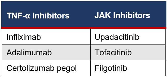 Table 1: Summary of Current Treatment Options for CD patients. Source: “Medical Management of Crohn’s Disease”. (2020) Cureus
Table 2: The specific inhibitors considered for this review.
Table 1: Summary of Current Treatment Options for CD patients. Source: “Medical Management of Crohn’s Disease”. (2020) Cureus
Table 2: The specific inhibitors considered for this review.
The Journal of Science Extension Research – Vol. 2, 2023 education.nsw.edu.au 66
Tumour necrosis factor (TNF) is a highly pro-inflammatory cytokine that induces fever, insulin resistance, bone resorption, anaemia, inflammation in CD and in sepsis. It is mainly produced by monocytes, macrophages and T lymphocytes, but also by mast cells, granulocytes, fibroblasts and several other cell types. (Tracey, D. et al. 2008).
TNF reacts with two distinct receptors (TNF receptor 1 [see figure 4] and TNF receptor 2) which exerts their biological effects, which include the increased production of proinflammatory cytokines and the inhibition of apoptosis of inflammatory cells (Sanchez-Muñoz, F. 2008).
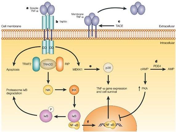
4
TNF-α inhibitors reduce the overexpression of TNF-α, by binding soluble and transmembrane TNF-α and inhibiting binding to its receptors (see figure 4), resulting in the blockage of proinflammatory signals. It also induces apoptosis of activated lamina propria T lymphocytes, countering a proposed pathological mechanism in CD, where mucosal T cell proliferation exceeds T cell apoptosis (Adegbola, S. 2018). TNF-α inhibitors have led to a paradigm shift in CD treatments, allowing rapid, sustained and deep remission. Short and long-term clinical and endoscopic endpoints can now be reached that were previously unachievable. (Rutgeerts, P. et al. 2012).
Figure 4: The basic mechanism of TNF-α inhibition. The binding of TNF to TNFRI and TNFRII (a) activates several signalling pathways. This signalling leads to activation of the target cell leading to the inflammatory and immune response by releasing several cytokines and apoptotic pathway initiation (b). SOURCE: “Nature Reviews Drug Discovery” and “StatPearls - TNF Inhibitors”
The Journal of Science Extension Research – Vol. 2, 2023 education.nsw.edu.au 67
4 Death of cells which occurs as a normal and controlled part of an organism's growth or development.
Examples of TNF-α inhibitors
Infliximab was the first biological response modifier to be used in the treatment of IBD and is a genetically engineered chimeric (mouse/human) immunoglobulin anti-human TNF agent. It can induce the downregulation of the inflammatory mechanisms in the entire mucosal area, by fixing complement and lyse cells that express membrane-bound TNF-α (D’Haens, G. et al. 1999). It is administered intravenously.
Adalimumab is a human immunoglobulin 5 antibody that also fixes complement and lyse cells that express TNF-α and is administered subcutaneously (via autoinjector pen) every two weeks (Rutgeerts, P. et al. 2012).
Certolizumab pegol is a chimeric humanized antibody fragment against TNF. Unlike infliximab and adalimumab, it does not contain the crystallisable fragment (Fc) region of a typical antibody. Its function is also different - it does not induce apoptosis as one of its mechanisms of action. It is thought to have a higher binding affinity 6 for TNF than adalimumab or infliximab (Adegbola, S. et al. 2018). CP is administered subcutaneously and has a longer half-life with maintenance dosing every four weeks (as opposed to adalimumab’s two weeks).
Issues
An issue often faced by clinicians and patients once remission has been achieved is whether to stop the anti-TNF therapy. Despite the multiple studies that have addressed this issue in Crohn’s Disease, no conclusive strategy has yet emerged (Adegbola, S. 2018).
There are up to 30% of primary nonresponders who do not respond to antiTNF therapy and almost half of the patients who experience a benefit with these drugs will lose clinical benefits within the first year, requiring dose escalation or therapy change. (Sandborn, W. 2007). Why this occurs is still discussed in the current literature and is an area for further research.
What are Janus Kinase (JAK) Inhibitors?
Janus Kinase (JAKs) are the enzymes that determine the signal transduction (process by which foreign DNA is introduced into a cell) by interaction with signal transducers and activators of the transcription (STATs) pathway (Dudek, P. 2021). It is named after Janus, the Roman god of doorways, to highlight how JAKs facilitate signals from the cell surface into the cell. JAK inhibitors are biologics, small molecules that prevent the signalling of many of the cytokines implicated in the pathogenesis of Crohn’s Disease, such as IL-6 and IL-23. Due to the different patient-to-patient specific cytokine profiles, widening the target of action to JAK-STAT pathways (see figures 5 and 6) is advantageous
5 A critical part of the immune response that specifically recognises and binds to particular antigens, such as bacteria or viruses, and aids in their destruction.
6 the strength of the binding interaction between a single biomolecule (e.g. protein or DNA) to its ligand/binding partner (e.g. drug or inhibitor).
The Journal of Science Extension Research – Vol. 2, 2023 education.nsw.edu.au 68
compared to selective biologic agents like TNF-α inhibitors. (Dudek, P. 2021).
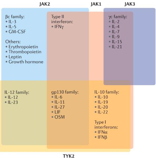
The Journal of Science Extension Research – Vol. 2, 2023 education.nsw.edu.au 69
Figure 5: Cytokine signalling through their respective JAKs. SOURCE: Nature Reviews Rheumatology
Mechanism of action
Figure 6:
1)
(usually a cytokine) binds and cross-links its receptor. 2) The associated JAKs transphosphorylate and activate each other. 3) The activated JAKs phosphorylate the receptor tail (introduce a phosphate group into a molecule or compound). 4) The receptor tail becomes a docking site for recruited STAT proteins, which themselves are phosphorylated by the activated JAKs. 5) The phosphorylated STATs dissociate from the receptor and dimerise. 6) STAT dimers translocate to the nucleus where they regulate gene transcription. SOURCE: “Basic Mechanisms of JAK Inhibition”. (2020). MEDITERRANEAN JOURNAL OF RHEUMATOLOGY
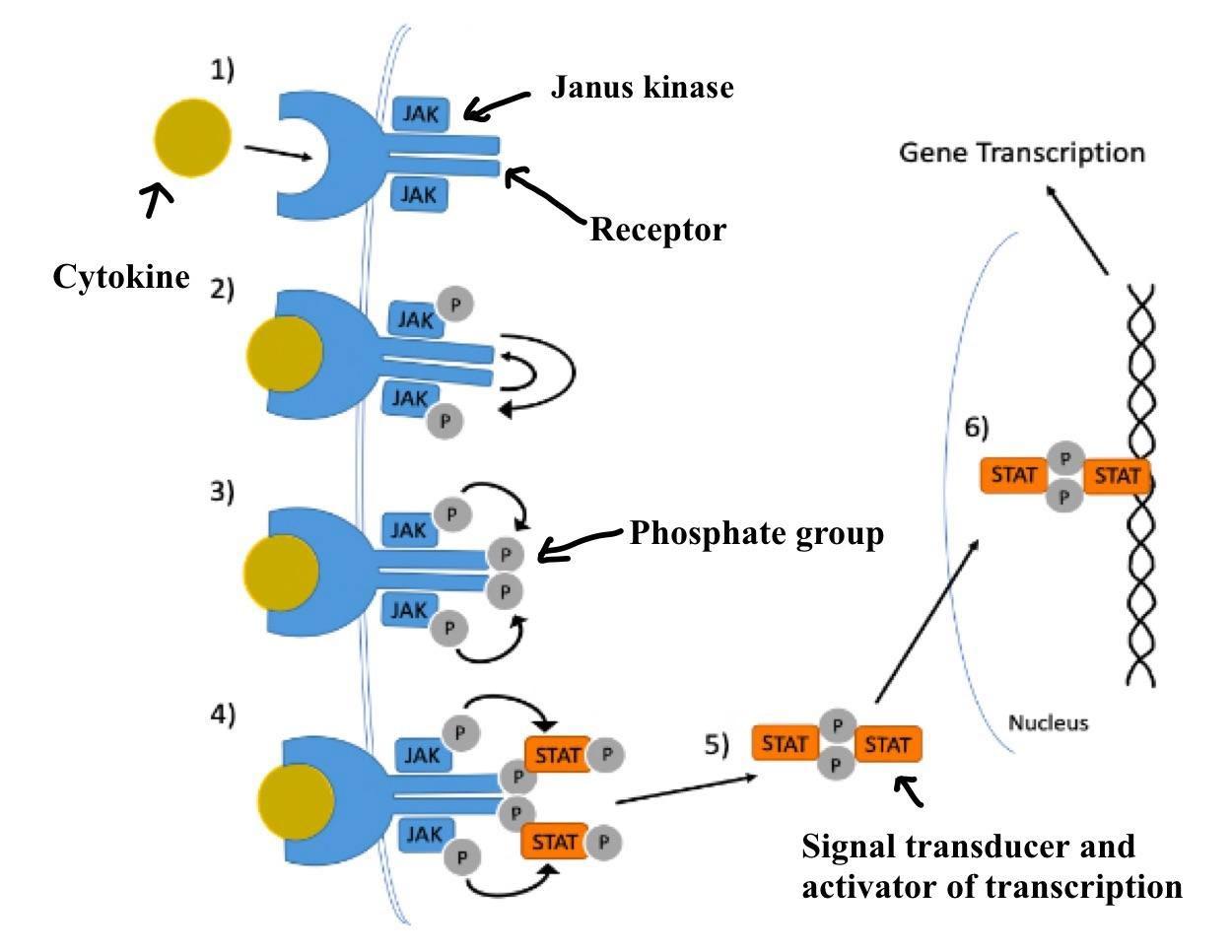
Overexpression of the JAK-STAT pathways is associated with both autoimmune disease and malignancy (Lin, C. et al. 2020). JAK inhibitors block these pathways, which simultaneously allows a blockade of multiple key cytokines associated with CD, thus reducing the severity of disease.
Examples of JAK Inhibitors
Current JAK inhibitors that are undergoing clinical trials for CD include tofacitinib, filgotinib and upadacitinib (table 2). Tofacitinib is a pan-JAK inhibitor that besides having a main activity for JAK1 and JAK3 also inhibits tyrosine kinases outside the JAK family, which
raises questions about whether its action can solely be attributed to JAK inhibition
A simplified diagram of the JAK-STAT Pathway.
Ligand
The Journal of Science Extension Research – Vol. 2, 2023 education.nsw.edu.au 70
(Rogler, G. 2020). Filgotinib is a selective janus kinase (JAK1) inhibitor with about 30 times selectivity for JAK1 over JAK2 in human whole blood (Vermeire, S. et al. 2016). Upadacitinib is a JAK1 inhibitor with increased selectivity for JAK1 compared with JAK2, JAK3, and TYK2, and down-regulates multiple proinflammatory cytokines, including interleukin(IL)-2, IL-4, IL-6 and interferon gamma, that are relevant to the pathogenesis of CD (Sandborn, W. 2020). All three are orally administered.
Issues
However, as JAK inhibitors in CD is an emerging field, there is uncertainty surrounding the ideal dosage to maximise efficacy and minimise adverse effects. Appropriate biomarkers to determine whether a failure to respond to JAK inhibitors is due to inadequate dosing or that the disease is not mediated by JAKdependent cytokines is an area for further research, as the precise tissue-specific roles of JAKs are incompletely understood.(Gadina, M. et al. 2019).
Another significant issue of JAK inhibitors in current clinical practice is the risk of thromboembolic events (i.e. blocking of blood vessel by a particle from blood clots), which is even greater in patients with COVID-19 (Dudek, P. 2021).
Scientific research question
The purpose of this study is to assess and compare the efficacy of three different types of JAK Inhibitors and TNFα inhibitors to determine which class of inhibitor is more favourable in treating adult (age 18+) patients with Crohn’s Disease.
This report aims to provide CD patients and healthcare professionals with a comparison between the two classes of inhibitors to assist them with their treatment options.
Methodology
1. Randomised clinical trials were found using PubMed using the search tags and settings:

The Journal of Science Extension Research – Vol. 2, 2023 education.nsw.edu.au 71
Figure 7: Settings used for the controlled PubMed search. “(Inhibitor drug name) Crohn’s Disease NOT recurrence”. Clinical Trial, Randomised clinical trial in last 15 years (20072022), Language set to English, age set to adults: 18+
Adalimumab, infliximab and certolizumab pegol were the TNF-α inhibitors considered for this report. These drugs are the most commonly used TNF-α inhibitors for CD patients and clinical trial reports for these were the most accessible given the resources available.
Tofacitinib, filgotinib and upadacitinib were the JAK-inhibitors considered for this report as they were the only JAKinhibitors that had investigated in clinical trials for CD patients.
Randomised clinical trial data was used to minimise bias, improving validity.
A time span of 2007 to 2022 inclusive was decided to find more relevant articles for the TNF-α inhibitors. In the case of infliximab, it was first approved by the US Food and Drug Administration (FDA) for treating Crohn’s disease in 1998. As these TNF-α inhibitors have been an aspect of the standard of care for a more extended period of time than the emerging field of JAK inhibitors, research articles for the TNF-α inhibitors within the last decade were scarce. Therefore a wider time span was necessary to acquire the research articles.
2. Articles were removed depending on:
a) Relevance (Crohn’s disease the main focus, not another disease + excluded articles only determining safety profiles)
b) Long term studies
c) Full article accessible through the University of Sydney or is free
d) Had a measure of remission, either by CDAI 7 scores or by endoscopy
e) Duplicate studies
Long term studies for TNF-α inhibitors could not be compared with JAK inhibitors as there was a lack of long term studies in the emerging field of JAK inhibitors, so long term studies were not considered for this study.
Following initial search on PubMed and Step 2, Infliximab - 1 result
Duplicates, irrelevant and inaccessible articles were excluded.
Adalimumab - 3 results
Duplicates, irrelevant and inaccessible articles were excluded.
Certolizumab pegol - 3 results.
19 results removed - duplicates, relevance (different disease, focused on safety profile)
Filgotinib - 1 Results
2 results removed - both for relevance (One focused on pharmacokinetics and the other on drug-drug interactions)
Tofacitinib - 2 Results.
2 results removed - both were duplicates
Upadacitinib - 2 Results.
2 results removed - both for relevance (one focused on Rheumatoid Arthritis and the other on quality of life and work productivity improvements)
7 Crohn’s Disease Activity Index - Determines the current severity (disease activity) of Crohn's disease using a points-based system
The Journal of Science Extension Research – Vol. 2, 2023 education.nsw.edu.au 72
3. Remaining articles were placed into a table (appendix 1) and efficacy was determined using the following criteria: significant clinical remission when compared to placebo, significant endoscopic remission when compared to placebo, safety profile and bioavailability.
Each of these efficacy criterias were then rated out of five for both inhibitor classes (tables 4, 5, 6 and 7) and compared.
4. A thorough review of the current literature is most appropriate given the time constraints and the resources available to a student.
The Journal of Science Extension Research – Vol. 2, 2023 education.nsw.edu.au 73
Figure 8: A flowchart of the methodology
Table 3: Rating and justification for the clinical remission (and clinical response, where mentioned) of JAK and TNF-α inhibitors
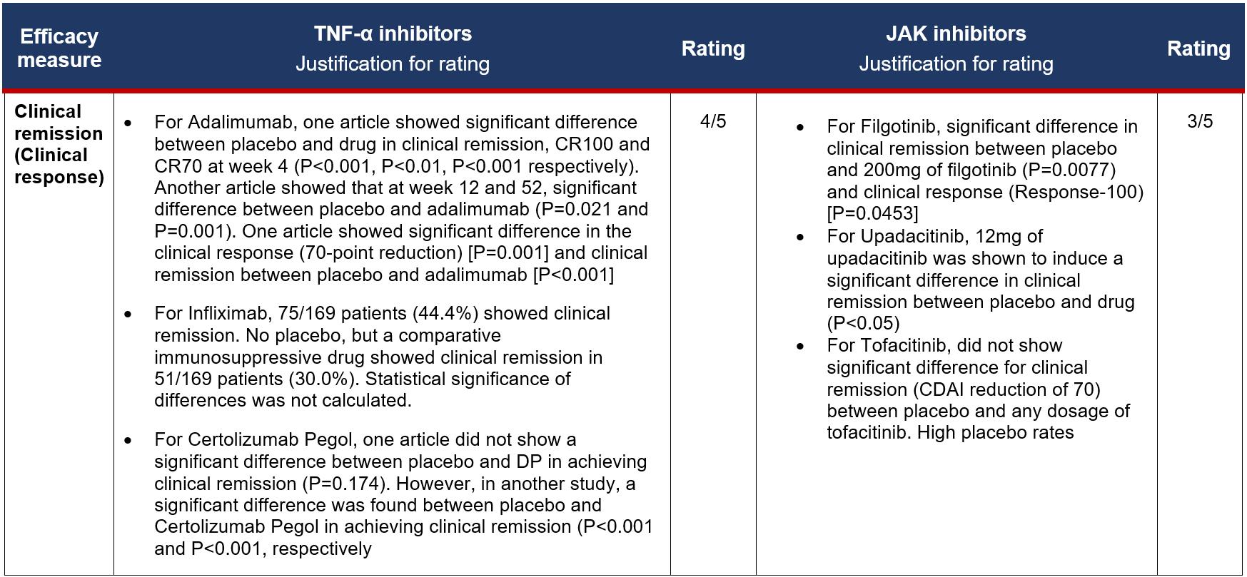
Results
The Journal of Science Extension Research – Vol. 2, 2023 education.nsw.edu.au 74
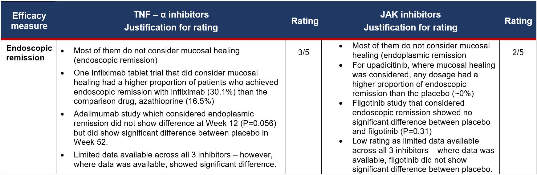
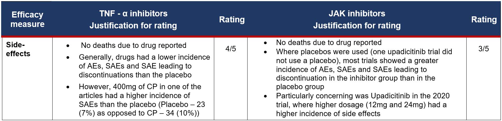 Table 4: Comparison between endoscopic remission in TNF-α inhibitors and JAK inhibitors
The Journal of Science Extension Research – Vol. 2, 2023 education.nsw.edu.au 75
Table 5: Ratings and justification for safety profile of TNF-α and JAK inhibitors
Table
Please refer to Appendix 1 for full results table.
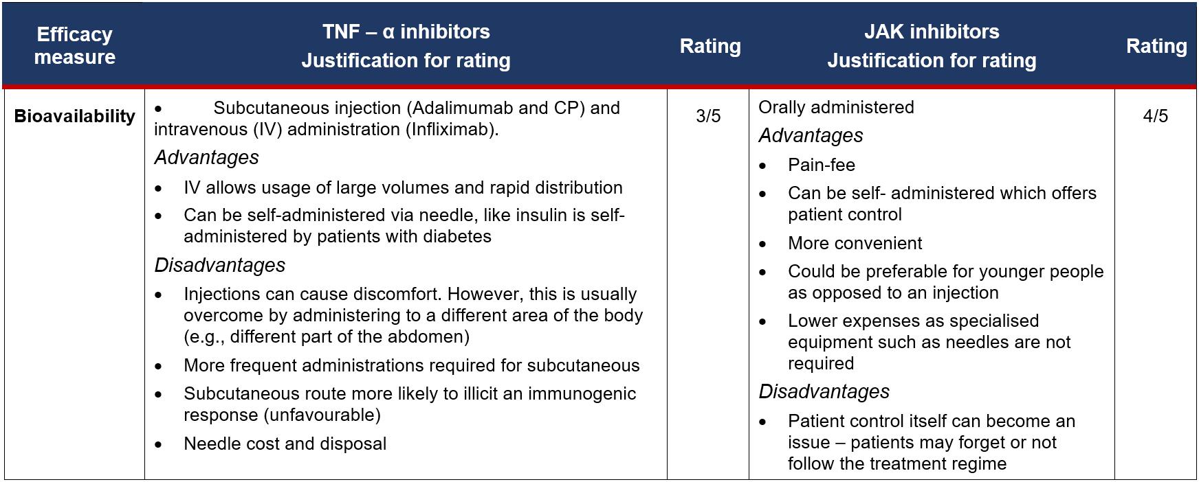 6: Rating and justification for bioavailability of TNF-α inhibitors and JAK inhibitors
The Journal of Science Extension Research – Vol. 2, 2023 education.nsw.edu.au 76
Discussion
Clinical remission
Clinical remission was defined as CDAI<150 for all studies. Not all studies considered clinical response, but the reports that did, considered CDAI-70 8 , CDAI-100 9 or both.
Adalimumab, infliximab and to a lesser extent, CP all showed a significant difference in clinical remission and, where it was included, clinical response. The double-blind, placebo-controlled “GAIN Study” for adalimumab showed a significant difference in clinical remission, CR100 and CR70 between adalimumab and placebo. However, the short 4-week duration 10 limited the study. The article was also very short, with no discussion and a brief explanation of methodology despite being published in the reputable AJG. 11
For JAK inhibitors, only Filgotinib and upadacitinib achieved a significant difference in clinical remission with placebo. The randomised, double-blind, placebo-controlled FITZROY trial for filgotinib showed a significant difference. However, it had a small sample size (n=128) and the data was inclusive i.e. some patients who achieved clinical response also achieved CR100, which may have overrepresented the findings.
However, the randomised, double-blind, placebo-controlled “Phase 2 study of Tofacitinib” did not show significant
differences in CR70, CR100 or clinical remission with placebo, with some P values greater than .999 for CR70 and CR100 due to small sample sizes. The short duration of 4 weeks limited the study, which was chosen to reduce placebo response rates. These rates were still high 12 and may be due to selection bias toward the enrollment of patients with a more benign natural history. (Sandborn, W.J. et al. 2014.). The study also could not determine if the failure of tofacitinib to show efficacy for CD was due to a high placebo response rate or a true negative result.
Subsequently, the clinical development of tofacitinib in CD was discontinuedhowever, it was still included due to the lack of JAK inhibitor trials for CD treatment and as it showed efficacy in ulcerative colitis (UC), another IBD.
Tofacitinib targets multiple JAK pathways while the other two are selective JAK Inhibitors. The pathways targeted and why the inhibition of those pathways worked for UC and did not work for CD is an area of further study. This could reveal why some cytokine pathways may be more responsible for disease activity in CD than others, which can provide further insight into the pathogenesis and pathophysiology of CD. (Rogler, G. 2019).
Endoscopic remission
Across the studies, most articles did not consider endoscopic remission as an endpoint, highlighting a clear limitation. 8
CDAI score
70
CDAI score
100 points
an induction therapy
of Gastroenterology
of placebo group achieved clinical remission The Journal of Science Extension Research – Vol. 2, 2023 education.nsw.edu.au 77
Reduction of
by
points 9 Reduction of
by
10 The trial was
11 American Journal
12 20.6%
Where it was considered, the same standardised measure was not used across all studies.
From the TNF-α inhibitors, adalimumab and infliximab were assessed for endoscopic remission. The randomised, double-blind, placebo-controlled “EXTEND” trial for adalimumab used mucosal healing 13 as a measure of endoscopic remission. At week 12, the difference between the remission rates was considered not statistically significant between placebo and adalimumab groups (P=0.056). However, at week 52, there was a significant difference between the placebo and inhibitor group (P<0.001). A limitation of this study in regards to the research question is its focus on the ileocolon, a specific part of the GI. More studies are needed to confirm endoscopic remission across different areas of the GI.
From the JAK inhibitors, endoscopic remission was measured for filgotinib and upadacitinib. The “FITZROY” filgotinib trial used SES-CD 14 to determine endoscopic remission in the placebo and filgotinib groups. There was no significant difference between the filgotinib and placebo groups after 10 weeks (P=0.31). However, due to the transmural 15 nature of CD, a longer treatment period may be required to achieve endoscopic remission (Vermeire, S. et al. 2016). Extended studies of filgotinib for CD patients are therefore required.
Safety profile
SAEs 16 included CD flares, sepsis and UTIs 17. While the studies determined that all six inhibitors had acceptable safety profiles, upadacitinib was concerning. SAEs were common in the randomised, blinded upadacitinib trial (Sandborn, W. et al. 2020), where all of the four doses displayed a higher incidence of SAEs than the placebo. In the 12 mg group, 25% of patients discontinued the treatment due to SAEs compared to the discontinuation of 13.5% of the placebo group. Two intestinal perforations were observed during the induction period. Intestinal perforations were initially reported with tofacitinib and may be related to an effect on IL-6, confirming its significance in the intestinal barrier. (Sandborn, W.J. et al. 2020). The study also found that intestinal perforation events occurred in areas of active intestinal inflammation of CD in patients treated with upadacitinib and corticosteroids, raising questions on whether combination therapy with upadacitinib is recommended in inducing remission for patients with active CD as opposed to maintaining remission.
Therefore, TNF-α inhibitors are preferable from a safety perspective at this time, although filgotinib is also a good alternative.
Bioavailability
Adalimumab and CP can be selfadministered via a needle, similar to how patients with diabetes inject insulin by
13 Ileocolonoscopy was used to determine if the ileocolon had ulcerations after treatment
14 Simplified Endoscopy Score for Crohn’s Disease
15 Existing or occurring across the entire wall of an organ or blood vessel.
17 Urinary tract infection
16 Severe adverse event
The Journal of Science Extension Research – Vol. 2, 2023 education.nsw.edu.au 78
themselves. However, as it does involve needles, immunogenecity 18 is a concern. (Adegbola, S. et al. 2018). Needle disposal and the costs associated with the equipment required are also other disadvantages to consider. Since the inhibitor is administered over a period of time (e.g. every 2 weeks) to induce or maintain remission, continuous injections can cause discomfort.
JAK inhibitors are orally administered and are pain-free. It can be self-administered which offers patient control and the lack of needles and other equipment make JAK inhibitors more convenient for patients. While this report does not focus on children and adolescents, JAK inhibitors could be preferable for younger people with CD as opposed to regular injections. Also, they were shown to exert no immunogenicity (Dudek, P. et al. 2021), an added benefit over TNF-α inhibitors.
Limitations
A limitation of this report is the lack of other efficacy measures, such as CRP levels and IBDQ which were not assessed. These other factors and biomarkers were not assessed due to time constraints. While this report still compares the efficacy of TNF-α inhibitors and JAK inhibitors, it does not capture the entire complexity of the inhibitor’s effects which limits its usefulness in providing advice for personalised treatment options for CD patients. Further studies into these factors and biomarkers can provide more insights into the inhibitors’ mechanism of action and guide treatment options.
More specificity for induction and maintenance treatments is also needed to narrow down the research question further, as results differed for maintenance and induction treatments. However, due to the lack of clinical trial data available for JAK inhibitors, a limitation of the field itself, this was not considered for the report. More clinical trials of JAK inhibitors in treating CD are therefore needed.
Limitations of the field include the lack of JAK inhibitor studies, small patient sample sizes for both classes of inhibitors, outdated TNF-α 19 studies and the lack of focus on endoscopic remission as a measured endpoint.
Future directions
To overcome the limitations of the field mentioned above, more trials should be conducted with larger patient sample sizes with a focus on endoscopic remission, which will significantly contribute to this field. Understanding why some JAK and TNF-α inhibitors work while others don’t through these clinical trials can reveal further insights into the various mechanisms of cytokines and JAK-STAT pathways, which can provide a greater understanding of the pathogenesis of CD.
Conclusion
While JAK inhibitors show promise in treating CD, TNF-α inhibitors remains as the gold standard for treatment, in terms of clinical remission and response, endoscopic remission and safety. A controlled PubMed search was conducted
18 Occurs when the immune system administered a drug recognises it as foreign and generates a cellular immune response. Can cause loss of response to treatments.
19 majority of studies were over 15 years ago, which could not be considered for this report.
The Journal of Science Extension Research – Vol. 2, 2023 education.nsw.edu.au 79
to gather articles that were analysed and synthesised into tables based on a set of efficacy criteria. The treatments were hen rated out of 5 for each criteria.
The benefits of oral administration of JAK inhibitors and the clinical and endoscopic remission in filgotinib and upadacitinib could not outweigh the discontinuation of tofacitinib due to the lack of clinical remission and the concerning safety profile of upadacitinib, and so failed to contend with the accepted TNF-α inhibitors. Therefore, TNF-α inhibitors are more efficacious than JAK-inhibitors in treating adult patients with CD.
Further investigations into the efficacy of these biologic treatments can improve patient care and lead to a better understanding of the pathology of CD.
Acknowledgements
I would like to thank Dr Dennis for her dedication and tireless support towards my project, without which I would not have been able to complete it.
I also thank Dr Vicki Xie for her valuable guidance and insightful comments in fleshing out the details of this report, for answering my questions and for teaching me the various clinical aspects of science.
I would also like to thank Mr Michael Chen for his valuable support in proofreading this report and for providing me with advice.
Bibliography
Adegbola, S.O. et al. (2018) “Anti-TNF therapy in Crohn’s disease,” International Journal of Molecular Sciences. MDPI AG.
Available at: https://doi.org/10.3390/ijms19082244.
Aguilar, D. et al. (2021) “Randomized controlled trial substudy of cell-specific mechanisms of Janus Kinase 1 inhibition with upadacitinib in the Crohn’s disease intestinal mucosa: Analysis from the CELEST study,” Inflammatory Bowel Diseases, 27(12), pp. 1999–2009.
Available at: https://doi.org/10.1093/ibd/izab116.
Ahluwalia, B. et al. (2018) “Immunopathogenesis of inflammatory bowel disease and mechanisms of biological therapies,” Scandinavian Journal of Gastroenterology. Taylor and Francis Ltd, pp. 379–389. Available at: https://doi.org/10.1080/00365521.2018.14 47597.
“Aliment Pharmacol Ther - 2010MEDDINGS - Review article Intestinal permeability in Crohn s disease” (no date).
Ananthakrishnan, A.N. (2017) “Filgotinib for Crohn’s disease expanding treatment options,” The Lancet. Lancet Publishing Group, pp. 228–229. Available at: https://doi.org/10.1016/S01406736(16)32538-7.
Choy, E.H. et al. (2020) “Translating IL-6 biology into effective treatments,” Nature Reviews Rheumatology. Nature Research, pp. 335–345. Available at:https://doi.org/10.1038/s41584-0200419-z
The Journal of Science Extension Research – Vol. 2, 2023 education.nsw.edu.au 80
Danese, S. et al. (2019) “Randomised trial and open-label extension study of an anti-interleukin-6 antibody in Crohn’s disease (ANDANTE I and II),” Gut, 68(1), pp. 40–48. Available at:
https://doi.org/10.1136/gutjnl-2017314562
D’Haens, G. et al. (2022) “Upadacitinib Was Efficacious and Well-tolerated Over 30 Months in Patients With Crohn’s Disease in the CELEST Extension Study,” Clinical Gastroenterology and Hepatology [Preprint]. Available at:
https://doi.org/10.1016/j.cgh.2021.12.030
Dudek, P. et al. (2021) “Efficacy, safety and future perspectives of jak inhibitors in the ibd treatment,” Journal of Clinical Medicine. MDPI. Available at:
https://doi.org/10.3390/jcm10235660.
Frédéric Colombel, J. et al. (2010) Infliximab, Azathioprine, or Combination Therapy for Crohn’s Disease Abstract.
Gade, A.K., Douthit, N.T. and Townsley, E. (2020) “Medical Management of Crohn’s Disease,” Cureus [Preprint].
Available at:
https://doi.org/10.7759/cureus.8351
Gadina, M. et al. (2019) “Janus kinases to jakinibs: From basic insights to clinical practice,” Rheumatology (United Kingdom), 58, pp. i4–i16. Available at:
https://doi.org/10.1093/rheumatology/key 432
Ito, H. et al. (2004) “A Pilot Randomized Trial of a Human Anti-Interleukin-6 Receptor Monoclonal Antibody in Active Crohn’s Disease,” Gastroenterology, 126(4), pp. 989–996. Available at:
https://doi.org/10.1053/j.gastro.2004.01.0 12.
Kany, S., Vollrath, J.T. and Relja, B. (2019) “Cytokines in inflammatory disease,” International Journal of Molecular Sciences. MDPI AG. Available at: https://doi.org/10.3390/ijms20236008
Lin, C.M., Cooles, F.A. and Isaacs, J.D. (2020) “Basic Mechanisms of JAK Inhibition,” Mediterranean Journal of Rheumatology, 31, pp. 100–1404.
Available at:
https://doi.org/10.31138/MJR.31.1.100.
Ljung, T. et al. (2004) “Infliximab in inflammatory bowel disease: Clinical outcome in a population based cohort from Stockholm County,” Gut, 53(6), pp. 849–853. Available at:
https://doi.org/10.1136/gut.2003.018515
Loftus, E. v. et al. (2016) “Safety of Longterm Treatment With Certolizumab Pegol in Patients With Crohn’s Disease, Based on a Pooled Analysis of Data From Clinical Trials,” Clinical Gastroenterology and Hepatology, 14(12), pp. 1753–1762.
Available at:
https://doi.org/10.1016/j.cgh.2016.07.019
Michielan, A. and D’Incà, R. (2015) “Intestinal Permeability in Inflammatory Bowel Disease: Pathogenesis, Clinical Evaluation, and Therapy of Leaky Gut,” Mediators of Inflammation. Hindawi Publishing Corporation. Available at:
https://doi.org/10.1155/2015/628157
Moon, W. et al. (2015) “Efficacy and safety of certolizumab pegol for Crohn’s disease in clinical practice,” Alimentary Pharmacology and Therapeutics, 42(4), pp. 428–440. Available at: https://doi.org/10.1111/apt.13288.
The Journal of Science Extension Research – Vol. 2, 2023 education.nsw.edu.au 81
Panés, J. et al. (2017) “Tofacitinib for induction and maintenance therapy of Crohn’s disease: Results of two phase IIb randomised placebo-controlled trials,” Gut, 66(6), pp. 1049–1059. Available at:
https://doi.org/10.1136/gutjnl-2016312735
Panés, J. et al. (2019) “Long-term safety and tolerability of oral tofacitinib in patients with Crohn’s disease: results from a phase 2, open-label, 48-week extension study,” Alimentary Pharmacology and Therapeutics, 49(3), pp. 265–276. Available at:
https://doi.org/10.1111/apt.15072
Peyrin-Biroulet, L. et al. (2021) “Quality of Life and Work Productivity Improvements with Upadacitinib: Phase 2b Evidence from Patients with Moderate to Severe Crohn’s Disease,” Advances in Therapy, 38(5), pp. 2339–2352. Available at:
https://doi.org/10.1007/s12325-02101660-7
Regueiro, M. et al. (2016) “Infliximab Reduces Endoscopic, but Not Clinical, Recurrence of Crohn’s Disease after Ileocolonic Resection,” Gastroenterology, 150(7), pp. 1568–1578. Available at:
https://doi.org/10.1053/j.gastro.2016.02.0
Roda, G. et al. (2020) “Crohn’s disease,” Nature Reviews Disease Primers, 6(1). Available at:
https://doi.org/10.1038/s41572-020-01562.
Rogler, G. (2020) “Efficacy of JAK inhibitors in Crohn’s Disease,” Journal of Crohn’s & colitis. NLM (Medline), pp. S746–S754. Available at:
https://doi.org/10.1093/ecco-jcc/jjz186
Rose-John, S., Winthrop, K. and Calabrese, L. (2017) “The role of IL-6 in host defence against infections: Immunobiology and clinical implications,” Nature Reviews Rheumatology Nature Publishing Group, pp. 399–409. Available at:
https://doi.org/10.1038/nrrheum.2017.83
Rutgeerts, P. et al. (2012) “Adalimumab induces and maintains mucosal healing in patients with Crohn’s Disease: Data from the EXTEND trial,” Gastroenterology, 142(5). Available at:
https://doi.org/10.1053/j.gastro.2012.01.0 35
Sanchez-Muñoz, F., Dominguez-Lopez, A. and Yamamoto-Furusho, J.K. (2008) “Role of cytokines in inflammatory bowel disease,” World Journal of Gastroenterology. Baishideng Publishing Group Co, pp. 4280–4288. Available at:
https://doi.org/10.3748/wjg.14.4280
Sandborn, W.J. et al. (2007).
“Adalimumab Rapidly Induces Clinical Remission and Response in Patients with Moderate to Severe Crohn's Disease Who Had Secondary Failure to Infliximab Therapy: Results of the GAIN Study.” American Journal of Gastroenterology.
Sandborn, W.J. et al. (2011)
“Certolizumab Pegol for Active Crohn’s Disease: A Placebo-Controlled, Randomized Trial,” Clinical Gastroenterology and Hepatology, 9(8). Available at:
https://doi.org/10.1016/j.cgh.2011.04.031.
Sandborn, W.J. et al. (2014) “A phase 2 study of Tofacitinib, an oral janus kinase inhibitor, inpatients with crohn’s disease,” Clinical Gastroenterology and Hepatology, 12(9). Available at:
https://doi.org/10.1016/j.cgh.2014.01.029
72
The Journal of Science Extension Research – Vol. 2, 2023 education.nsw.edu.au 82
Sandborn, W. J. et al. (2014) “Long-term safety and efficacy of certolizumab pegol in the treatment of Crohn’s disease: 7year results from the PRECiSE 3 study,” Alimentary Pharmacology and Therapeutics, 40(8), pp. 903–916.
Available at:
https://doi.org/10.1111/apt.12930
Sandborn, W.J. et al. (2020) “Efficacy and Safety of Upadacitinib in a Randomized Trial of Patients With Crohn’s Disease,” Gastroenterology, 158(8), pp. 21232138.e8. Available at:
https://doi.org/10.1053/j.gastro.2020.01.0
47
Sandborn, W.J. et al. (no date) Certolizumab Pegol for the Treatment of Crohn’s Disease Abstract Available at: www.nejm.org.
Schreiber, S. et al. (2021) “Therapeutic Interleukin-6 Trans-signaling Inhibition by Olamkicept (sgp130Fc) in Patients With Active Inflammatory Bowel Disease,” Gastroenterology, 160(7), pp. 23542366.e11. Available at:
https://doi.org/10.1053/j.gastro.2021.02.0
62.
Schreiner, P. et al. (2019) “MechanismBased Treatment Strategies for IBD: Cytokines, Cell Adhesion Molecules, JAK Inhibitors, Gut Flora, and More,” Inflammatory Intestinal Diseases, 4(3), pp. 79–96. Available at:
https://doi.org/10.1159/000500721
Siegmund, B. and Danese
Gastroenterology, S. (1999) Regulatory approval dates a. Tanaka, T., Narazaki, M. and Kishimoto, T. (2014) “Il-6 in inflammation, Immunity, And disease,”
Cold Spring Harbor Perspectives in Biology, 6(10). Available at:
https://doi.org/10.1101/cshperspect.a016 295.
Sultan, K. S., Berkowitz, J. C., & Khan, S. (2017). Combination therapy for inflammatory bowel disease. World journal of gastrointestinal pharmacology and therapeutics, 8(2), 103–113. Available at:
https://doi.org/10.4292/wjgpt.v8.i2.103
Teshima, C.W., Dieleman, L.A. and Meddings, J.B. (2012a) “Abnormal intestinal permeability in Crohn’s disease pathogenesis,” Annals of the New York Academy of Sciences, 1258(1), pp. 159–165. Available at:
https://doi.org/10.1111/j.17496632.2012.06612.x
Tracey, D. et al. (2008). “Tumor necrosis factor antagonist mechanisms of action: A comprehensive review”. Pharmacol. Ther.117, 244–279. Available at: 10.1016/j.pharmthera.2007.10.001
Vermeire, S. et al. (2017) “Clinical remission in patients with moderate-tosevere Crohn’s disease treated with filgotinib (the FITZROY study): results from a phase 2, double-blind, randomised, placebo-controlled trial,” The Lancet, 389(10066), pp. 266–275.
Available at:
https://doi.org/10.1016/S01406736(16)32537-5. Wallace, K.L. et al. (2014) “Immunopathology of inflammatory bowel disease,” World Journal of Gastroenterology, 20(1), pp. 6–21.
Available at:
https://doi.org/10.3748/wjg.v20.i1.6.
The Journal of Science Extension Research – Vol. 2, 2023 education.nsw.edu.au 83

1 The Journal of Science Extension Research – Vol. 2, 2023 education.nsw.edu.au 84
Appendix
The impacts of eye drop storage conditions on the microbial growth of eye surfaces
Rosie Kerruish Willoughby Girls High School
Increasing eye-related concerns in patients has led to a heightened need for treatments in the form of over-the-counter eye lubricants. The misconduct in the storage of these medications is known to increase the microbial contamination of the bottles and solutions, however, the impacts on the eye were yet unknown. This study aimed to investigate how differing storage conditions of eye drop bottles affected the microbial growth on eye surfaces. This was done by manually counting the number of microbial colonies on nutrient agar cultures of normal, open, half-open and expired eye drop bottles and treated cows’ eye surfaces. It was found that moving away from the standardised storage conditions of eye drop bottles produced greater microbial growth on cow’s eyes. Expired eye drops cultured the highest number of colonies, both in the bottle and on the treated eye surface. The averages of all growths were plotted to determine the R2 value, which was found to be 0.938, indicating a very strong, positive correlation between the variables. Thus, the correct storage of eye drops has high importance to prevent or limit microbial growth on patient eye surfaces.
Literature Review
Tetrahydrozoline
Tetrahydrozoline (C13H16N2) is a decongestant drug due to its induction of vasoconstriction, the temporary narrowing of blood vessels, in the nose and conjunctiva. This occurs from an imitation of the sympathetic nervous system on adrenergic transmission, which involves adrenergic nerve tissue using adrenaline, noradrenaline or dopamine neurotransmitters across neuron synapses (Farzam, et al., 2022). Without decongestant drugs, alpha-adrenergic receptors (α1-receptors) found at the postsynaptic target cells naturally bind to these neurotransmitters (Perez, 2020). However, the introduction of α1-receptors agonists, including tetrahydrozoline (THZ), can mimic neurotransmitters to
activate receptors (Hosten and Snyder, 2020), stimulating the same contraction of the inner layer of blood vessels, vascular endothelial cells, causing vasoconstriction. Due to this, THZ is typically found in eye drops treating burning and irritation in eyes in the form of Tetrahydrozoline HCl 0.05%, from such vasoconstriction, narrowing the prominent blood vessels. The disorder of red eyes is most commonly associated with bacterial infections such as conjunctivitis and can result in discharge, prominent red blood vessels, pain, itching and blurry vision. Dry eye is an abnormality in lacrimal gland activity that reduces secretion of lacrimal fluid, the supply of lubricating fluids, to the conjunctival fornix and cornea. Sympathetic nerves in lacrimal glands stimulate the ocular surface for tear production (Conrady, et al., 2016), meaning that THZ can again act as α1-
The Journal of Science Extension Research – Vol. 2, 2023 education.nsw.edu.au 85
receptors agonists, artificially replicating the acetylcholine and norepinephrine neurotransmitters. These send chemical and electrical signals to duct cells to regulate and produce lacrimal gland protein secretion, relieving dry eye symptoms (Bhattacharya, et al., 2018). It was found that the most frequent ocular disorder primary care physicians encounter is red eye and dry eye (Leibowitz, 2000, Wirbelauer, 2006), underlining their significance in medicinal research, particularly in synthesising and understanding treatments, including THZ.
Microbial Contamination in Eye Drop Bottles
The frequency of microbial contamination within eye drop bottles has been assessed from hospital and pharmaceutical company samples, with rates ranging from 5.3% (Teuchner, et al., 2015) to 45.9% (Feghhi, et al., 2008). The 2015 Teuchner study compared different types and brands of eye drops, outside the defined independent variable, which restricts the validity of the experiment due to a lack of controlled variables. Additionally, the study focused on the percentage of contaminated eye drops and did not go into further detail surrounding the specific storage conditions affecting bacterial growth, despite its significant contribution to the results. This inconsistency means that additional research must be conducted to understand the factors that affect microbial growth in eye drop bottles. The shelf life of unopened and opened Autologous Serum Eye Drops (ASEDs) has been found to be between 1 to 6 months and 3 hours to 1 week, respectively, (Lee, et al., 2014). As well as this, a 2001 study found the contamination rate of eye drop bottles to
be 10.2% in unopened bottles and 34.8% in opened bottles, (Taşli and Coşar, 2001). These differing rates highlight the importance of closing eye drop bottles to both preserve eye solutions and potentially decrease microbial contamination, however, both the 2014 and 2001 studies focused on other active ingredient-based eye solutions in place of THZ. Staphylococcus aureus (S. aureus), a natural flora found in the nasal cavity and skin surface, has the highest contamination rate (Tsegaw, et al., 2017, Nisar, et al., 2018) in eye drop bottles than other bacterial colonies, due to accessible transfer from skin to bottles. Kruszewska (2006) exhibited THZ’s ability to inhibit S. aureus growth, in concentrations of 0.05 mg/ml, however, this is significantly below the 5-100 mg/ml concentrations of other non-antibiotic drugs. This is due to THZ’s ineffective prevention of translation as part of bacterial polypeptide synthesis, as it struggles to bind to a ribosomal aminoacyl active site in place of the bacterial amino-acyl tRNA. Kruszewska’s study did not include findings on the likelihood of contamination of THZ, rather it focuses on its general antimicrobial properties, meaning there is limited knowledge surrounding the conditions in which THZ products have increased microbial growth and how this may affect treated eyes. No similar studies have been conducted in relation to any microbial growth virulence in THZ solutions, which leaves an opening for further research, specifically surrounding the introduction of undesirable microbes to such THZ products. The studies suggested THZ’s lesser antibiotic properties, indicating the increased potential for contamination of tetrahydrozoline products.
The Journal of Science Extension Research – Vol. 2, 2023 education.nsw.edu.au 86
Microbial Growth on Eyes
Dry eyes has been shown to increase the prevalence of microbes on eye surfaces due to the lack of antibacterial lacrimal fluid coverage, including S. aureus and other closely related bacterial species. This occurs as a result of a significant decrease in immunoglobulin A (IgA), an antibody produced by plasma b cells in mucous membranes, and an increase in harmful lipase activity and toxins from ocular bacteria, causing cellular damage (Li, et al., 2019). Dry eyes inducing an increased microbial ocular growth, combined with THZ’s limited antimicrobial activity producing contaminated eye drop bottles, significantly increases the chances of disease, such as keratitis, blepharitis and endophthalmitis. Many studies have injected bacteria samples directly into the conjunctival sac or cornea (O’Callaghan, 2018) to determine the effects, however, there are minimal methodologies surrounding surface level contamination, due to time constraints. In relation to other external sources infecting the ocular surface with microbes, contaminated contact lenses’ impact on ocular health has been thoroughly researched. Contact lenses act as vectors for microorganisms to adhere to the cornea and transfer to the internal elements of the eye (Shin, et al., 2016). However, there are few studies within the past two decades that relate to eye drops as vectors for microbes, and minimal information is available regarding the species and number of any such microorganisms.
The incorrect storage conditions of eye drop solutions have been shown to increase the contamination rate of many bottles in specific settings, however, studies lack depth on further applications
of this information. There are many connections yet to be discovered between contaminated THZ eye drop bottles and growth on treated eye surfaces, leaving a gap in scientific research regarding this correlation.
Research Question
How do tetrahydrozoline eye drops held in non-standardized conditions affect the microbial growth on eyes?
Hypothesis
As microbial growth increases inside eye drop bottles with a greater risk of pathogen contamination, microbial growth on treated eye surfaces will increase.
Methodology
Preparation of Eye Drop Bottles:
Four 15mL Visine(R) Red Eye Comfort eye drop bottles were collected for the Tetrahydrozoline HCl 0.05% active ingredient. One eye drop bottle was stored according to all safety instructions on the product box and was labelled “Bt 1” (indicating Bottle 1) with a permanent marker. A second bottle was stored according to all safety instructions on the product box, however, the lid was placed onto the nozzle, not screwed on and labelled “Bt 2”. A third bottle was stored according to all safety instructions on the product box, however, the lid was left off, placed next to the bottle and labelled “Bt 3”. A fourth bottle was stored according to all safety instructions on the product box, however, had expired for five months and labelled “Bt 4”. The four eye drop bottles were stored together for five weeks in a cool, dry cupboard before the study began.
The Journal of Science Extension Research – Vol. 2, 2023 education.nsw.edu.au 87
Preparation of Nutrient Agar plates:
800mL of water was measured at eye level using a 1L measuring cylinder which was poured into a 2L beaker on a hotplate set to maximum heat output. Four solid beef stock cubes were added and stirred using a plastic stirring rod for 3 minutes or until dissolved to make the beef broth. Two sterilised spatulas weighed 50g of salt and 50g of sugar to a watch glass on an electronic balance, to then be added to the broth. This solution was heated until the boiling point where 15g of solid agar, measured by the electronic balance, was added and stirred until dissolved. This solution was transferred to a 750mL autoclave bottle, where any excess not evaporated during boiling was poured down a suitable drain. The solution was sterilised overnight in an Autoclave and was collected the next morning using heat-resistant gloves. Antibacterial dish soap was combined with water to clean and rinse 20 plastic Petri dishes. The agar solution was then poured from the autoclave bottle into each Petri dish until three-quarters of the plate was full. The lids were immediately placed onto the agar plate to prevent air contamination and were left for 10 minutes to solidify, before being placed upside down in a refrigerator. One agar plate was placed in an incubator at 30oC for 72 hours to determine if any contamination occurred during preparation.
Data Collection:
Figure 1. Method of culture swab
Four cotton swabs were dipped in sterile water to dampen. These each swabbed one of the four eye drop bottles; in the lid, around the rim of the nozzle for thirty seconds and a single drop from the eye solution. These were cultured onto separate agar plates using three short zig-zag patterns, decreasing the pressure of the swab each time. Refer to Figure 1. They were then sealed with two layers of masking tape and labelled “1” (indicating bottle 1), “2”, “3” and “4”, respectively, with a permanent marker. These were left in an incubator upside down at 30oC for seventy-two hours. After these plates were stored, five cow eyes were placed into a container, where three drops of each bottle were added to a cow eye, leaving one eye with no additional eye drop solution. Each cow eye was labelled 1 through to 5 using a permanent marker on the side of the container, which was sealed and placed into a refrigerator. The next day the cow eyes were removed from the refrigerator, swabbed again using damp cotton swabs and cultured onto agar plates using the same method (Figure 1), being labelled “Eye 1” through to “Eye 5”. These were left in an incubator at 30oC for seventy-two hours. Three more drops of each bottle were added to the eyes before being stored again in the refrigerator. This was repeated for one more day. After the final swab, the cow
The Journal of Science Extension Research – Vol. 2, 2023 education.nsw.edu.au 88
eyes were placed in a ziplock bag and safely disposed of in a bin.
Data Analysis:
After seventy-two hours, each culture was taken out of the incubator and photographed. The size, shape, colour and number of each type of growth were counted and arranged into qualitative data in a table. The total number of observable colonies was counted for each agar culture, meaning that only the distinct colonies were recorded. A column graph was produced to graphically represent both the averages of the number of colonies in the eye drop bottles as well as the number of colonies on the cow’s eyes. Using excel, a single factor ANOVA test was conducted to find if there was a statistical significance
Results:
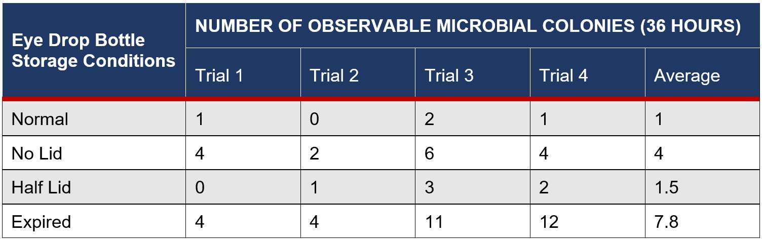
between microbial growth in both the eye drop bottles and the cow’s eyes as well as the variance in each data set. If a statistically significant result was found, individual two-sample unpaired T-tests were run between groups, using ‘assuming equal variances’ or ‘assuming unequal variances’ where applicable. A scatter plot was also generated between the number of colonies in the bottles versus the eyes to produce Pearson’s Correlation Coefficient to determine the strength of the relationship between the variables.
Experimental Repetition:
The whole study was repeated four times to check for reliability, using different eye drop bottles and cow’s eyes in each repetition.
Table 1: Number of Colonies in Eye Drop Bottles after 72 Hours
The Journal of Science Extension Research – Vol. 2, 2023 education.nsw.edu.au 89

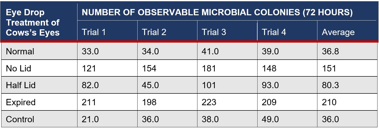
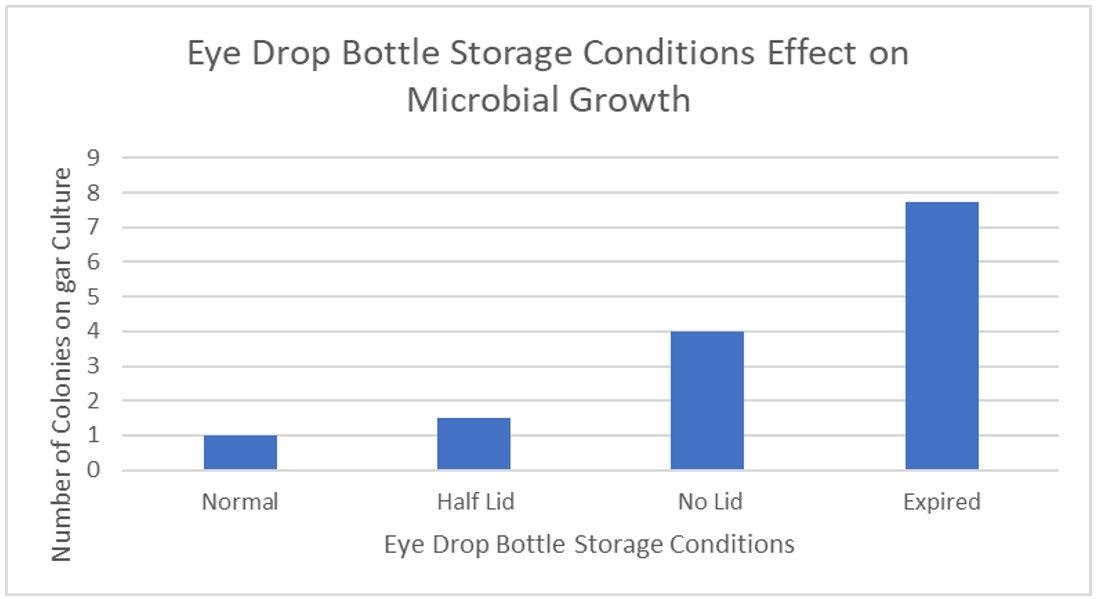 Figure 2: Average Number of Colonies of Microbes For Different Storage Conditions of Eye Drop Bottles
Table 2: Number of Colonies on Cows’ Eyes with Treatment From Eye Drop Bottles after 72 Hours
Figure 2: Average Number of Colonies of Microbes For Different Storage Conditions of Eye Drop Bottles
Table 2: Number of Colonies on Cows’ Eyes with Treatment From Eye Drop Bottles after 72 Hours
The Journal of Science Extension Research – Vol. 2, 2023 education.nsw.edu.au 90
Figure 3: Average Number of Colonies of Microbes For Cows’ Eyes Treated with Differently Stored Eye Drops
Table 3: Average Qualitative Results of Physical Characteristics of Microbes on Cow’s Eyes after 72 Hours
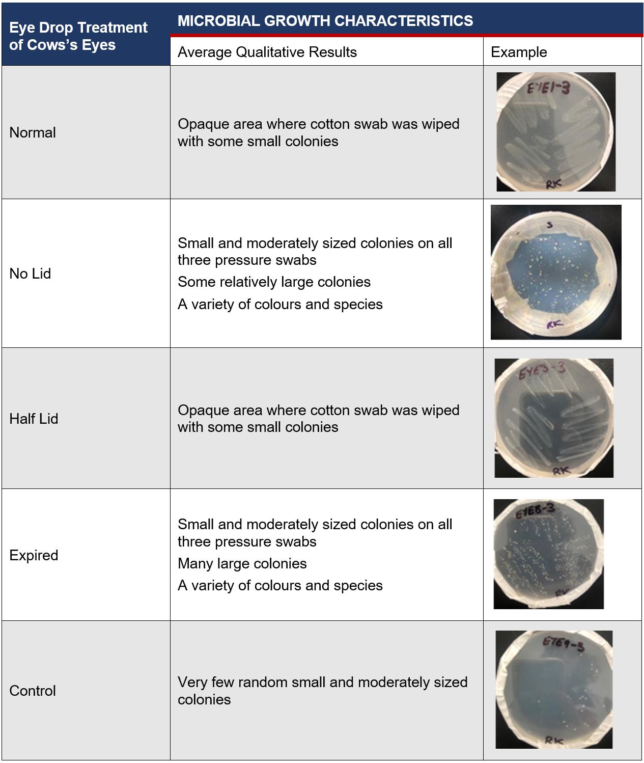
The Journal of Science Extension Research – Vol. 2, 2023 education.nsw.edu.au 91
Statistical Analysis
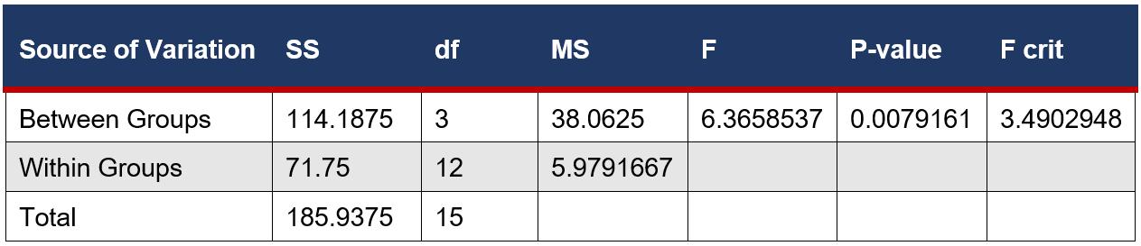
Eye Drop Bottles Test:
Alpha Significance Level = 0.05
H0: There is no statistical significance in the means of the microbial growth of the eye drop bottles across different storage conditions
H1: There is a statistical significance in the means of the microbial growth of the eye drop bottles across different storage conditions
An ANOVA Single factor test was used to determine if there was a significant difference between the means of the number of microbial colonies in eye drop bottles. This is a suitable test as there are more than two samples.
SUMMARY
This was followed by 2 sample, unpaired T-tests between each variable assuming equal variance from the ANOVA Single Factor test. This is a suitable test as it compared the means between individual groups and such groups were not related.
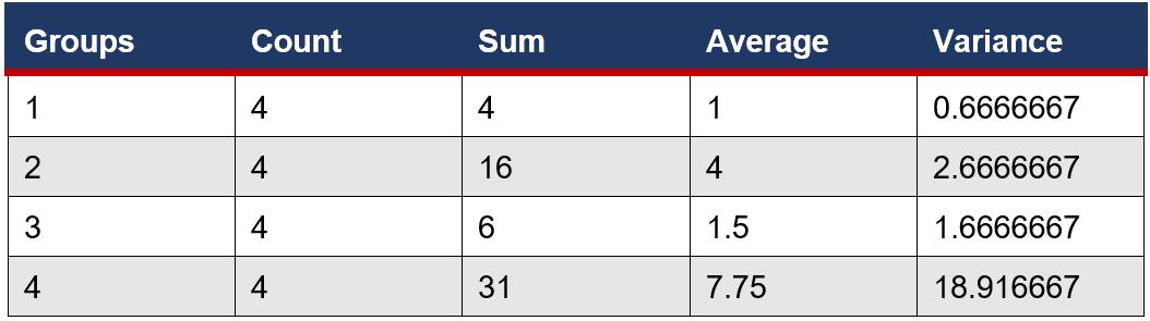 Figure 4: ANOVA single factor test performed on the microbial growth of different eye drop bottles
ANOVA
The Journal of Science Extension Research – Vol. 2, 2023 education.nsw.edu.au 92
Table 4: Summary of the Statistical Difference Between Eye Drop Bottle Storage Conditions and Microbial Growth
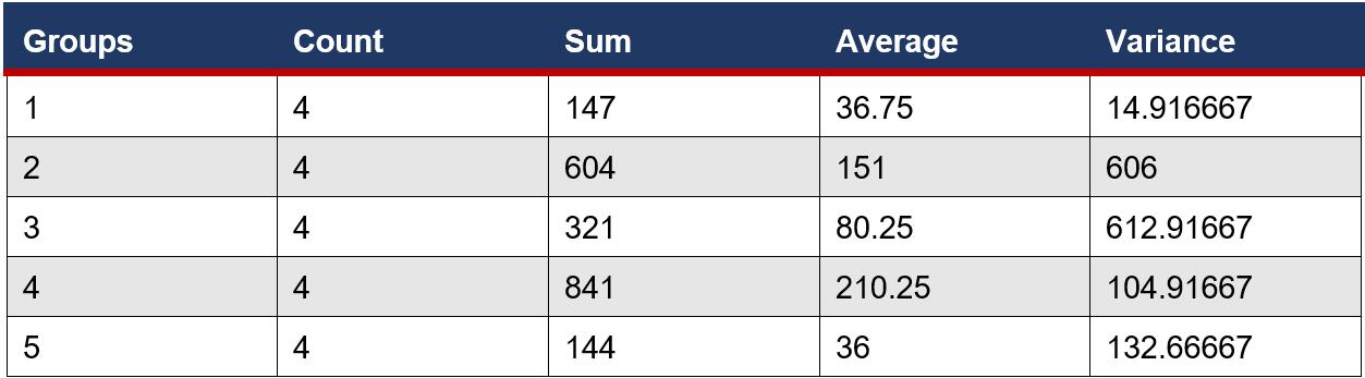
Cows’ Eye Test: Alpha Significance Level = 0.05
H0: There is no statistical significance in the means of the microbial growth on the cow eyes treated with of eye drops in different storage conditions
H1: There is a statistical significance in the means of the microbial growth on the
cow eyes treated with of eye drops in different storage conditions
An ANOVA Single factor test was used to determine if there was a significant difference between the means of the number of microbial colonies on eye surfaces. This is a suitable test as there are more than 2 samples.
SUMMARY
 Figure 5: ANOVA single factor test performed on the microbial growth of on cows’ eyes
The Journal of Science Extension Research – Vol. 2, 2023 education.nsw.edu.au 93
This was followed by 2 sample, unpaired T-tests between each variable assuming equal or unequal variances, depending on the given variance from the ANOVA Single Factor test. This is a suitable test as it compared the means between individual groups and such groups were not related.
Correlation Between Variables:
A Pearson Correlation was used to analyse the relationship between the growth of microbes inside the eye drop bottle and the subsequent growth on cows’ eyes. The averages were plotted against each other to determine the R2 value.

ANOVA
Table 5: Statistical Difference Between Eye Drop Bottle Groups for Microbial Growth on Eyes
The Journal of Science Extension Research – Vol. 2, 2023 education.nsw.edu.au 94
Discussion
This study aimed to show the relationship between microbial growth inside eye drop bottles stored in varying conditions and growth on eye surfaces. Stagnant liquids are ideal conditions for processes of binary fission and spore reproduction, meaning that open eye drop solutions, especially that of THZ with low antimicrobial properties, will produce more growth than bottles stored with the lid both thoroughly and partially closed. Furthermore, exposure to oxygen can accelerate the degeneration of chemical ingredients, causing the weakening of antimicrobial properties, exhausting essential processes, including vasoconstriction, and decreasing expiration dates. The open eye drop bottle versus the normal bottle had the only statistically significant result (Table Figure 6F4), meaning that the microbial growth is directly impacted by the storage conditions, not due to random chance. Eye drops that have already expired have undergone physical and chemical degradation, including oxidation and decarboxylation (Inam and Batool, 2017).
This chemical change alters the properties of THZ, where long periods of time allow multiple stages of oxidation to occur and an increased risk of microbial contamination. This correlated with experimental results, the expired eye drops having the highest microbial growth with an average of 7.8 (Table 1), due to this fundamental deterioration and greater susceptibility to growth. However, as a result of the high variance between trials, 18.9 (Figure 4), there was no statistical significance with other variables, meaning that it has no meaningful impact on microbial growth.
The placement of eye drops onto the surface of cows’ eyes allows microbes inside eye drop solutions to transfer and absorb into the eye, increasing contamination of the cornea. This suggests that increasing the microbial growth inside eye drop bottles will increase the growth in eyes, supported by the found R2 value of 0.938 (Figure 6), indicating that 93.8% of the variance within the growth is explained by the different storage conditions of eye drop bottles. This is seen in the expired eye
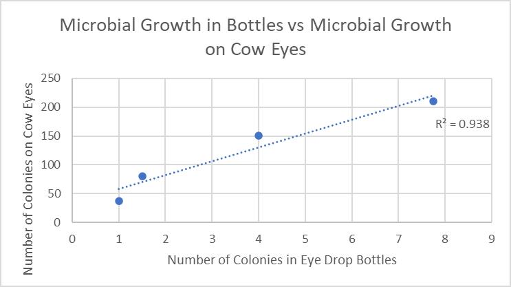 Figure 6: Growth in Eye Drop Bottles Plotted Against Growth on Cows’ Eyes
The Journal of Science Extension Research – Vol. 2, 2023 education.nsw.edu.au 95
drops producing the highest average of 210 colonies on the eye (Table 2), from the transfer of its high growth within the bottle. This value was compared against other bottles’ influence on microbial growth in eyes and a statistically significant outcome was found between each group (Table 5), indicating that there is a correlation between growth in eyes and contamination inside eye drop bottles. Furthermore, the expired eye drops had the greatest variety of colour, size and type of microbial colonies, indicating its high virulence rate. While the control experiment, the eye without solution, did produce microbial growth, this was expected due to the high contamination rate of raw meat in the agricultural industry (Bantawa, et al., 2018). This growth, 36 colonies (Table 2), is notably less than the growth from the no lid, half lid and expired treated eyes, producing a statistically significant difference for each one. However, the control had no statistical significance to the eye treated with eye drops stored under normal conditions, attributable to the lesser growths inside both bottles. The normal bottle had an average of 1 colony (Table 1), indicating low contamination from limited exposure to pathogens in the air, meaning it transfers few microorganisms across to the eye during treatment. Similarly, tetrahydrozoline’s limited antibiotic properties would not prevent nor restrict growth, indicating its similarity to the control experiment.
Accuracy:
The results from this experiment were compared to expected values from secondary resources and the identified trend was found to be very accurate. The linear regression figure between the two
variables, R2 = 0.938 (Figure 6), was exceptionally high indicating a very strong, positive correlation, which reflects expected results that increased exposure to pathogens within bottles increases growth on treated eyes. The equipment was accurate to determine microbial growth, using an electronic balance and a measuring cylinder with small error margins of 0.01g and 5mL, respectively. Parallax error did not affect water volume in the measuring cylinder, as measurements were taken at a flat angle. However, total counts of microorganisms were lower than expected, and this is most likely due to a combination of limited sensitivity of manual counting and the use of cows’ eyes. Despite this decreased value of microbe colonies, this study is concluded to be accurate due to the correct correlation identification and the use of precise equipment and techniques.
Reliability:
Four trials were conducted for each of the eye drop bottles and cow eye samples to check for reliability in the results. Very consistent data was obtained from eye drop bottle storage conditions trials, with the expired eye drops having the highest variance of 18.9. Moderately consistent data was obtained from the cow eyes trials, with the open eye drops having the highest variance at 613 (Figure 5) and a range of 60 (Table 2). However, this is expected due to microbial growth having a known high variability, with multiple factors affecting development of different organisms. An average was taken between the four trials to overcome this high variance, producing an accurate linear relationship. The sample size of this study was moderate, using four storage conditions and five treatments of cow eyes. Due to the consistent results in
The Journal of Science Extension Research – Vol. 2, 2023 education.nsw.edu.au 96
each data range, it can be concluded that this study was reliable.
Validity:
The controlled variables include, but are not limited to, the type of agar plate cultured, the time spent in the incubator, the set temperature of the incubator, location of sourced cows' eyes, and the culturing method. A control experiment was used to see if any contamination had occurred, allowing the plate to incubate normally, and no colonies were identified. A control experiment was utilised for the cow eye trials, with one eye having no eye drops added, to determine that the drops were increasing the microbial growth. The method of this study was valid as the independent variable of the storage conditions of eye drop bottles was changed and the dependent variable of the microbial growth on treated cow eyes was measured appropriately using manual counting of observable microbe colonies. There were some colonies that were too small to be accurately measured, meaning that they were discounted, however, this method was held constant for each plate, meaning that it is valid in its consistency. Due to the accurate results and valid methods, it can be concluded that this study was valid.
Limitations/Errors and Improvements:
Deceased cow eyes are utilised due to ethical and health concerns of human eye experimentation, however, there are a variety of differences between them. The number of microbial colonies found, a maximum of 210 (Table 2), was significantly lower than the predicted 0.06 bacteria per conjunctival cell (Shivaji, 2022), for each of the 50 million cells on
the eye surface. This may be attributed to a lack of sensitive equipment, however, this large range indicates another variable influencing the results, which is likely attributable to the use of cow eyes instead of human eyes. Cow eyes can be more resistant to S.aureus due to the Panton-Valentine Leukocidin (PVL) toxin, a secreted polypeptide that increases the virulence potential in hosts, present in approximately 5% of S.aureus colonies. PVL toxins bind to anaphylatoxin chemoreceptors, which are protein byproduct receptors that mediate acute inflammatory processes, to disrupt such processes, such as neutrophil differentiation into B, T and dendritic cells. Cow neutrophils are resistant to PVL toxins, whereas human cells are not (Astley, et al., 2019), indicating a potential for negatively skewed results, with the total capacity of bacteria not being grown on the cow’s eyes where it would on human eyes.
• The use of animal eyes more closely related to humans, such as monkeys or chimpanzees, should be used to prevent systematic errors in the prevention of microbial growth. If ethical parameters are managed, deceased human eyes could be used to produce the most accurate data.
The measurements of microbial growth were taken by counting the colonies on agar plates, meaning that small or indistinguishable colonies were not recorded.
• Automated microbe counters are machinery that counts microscopic colonies with much greater precision than the naked eye. Smartphone apps are being developed that allow microscopic
The Journal of Science Extension Research – Vol. 2, 2023 education.nsw.edu.au 97
and macroscopic counting of colonies on agar plates, therefore, future research may use cheap and accurate measurement methods
(Austerjost, et al., 2017)
The agar method was changed for trials 3 and 4 due to limited time and inaccessibility to an autoclave, meaning that the solution was not sterilised and there was an increased chance of contamination. This can be seen in the microbial growth of expired eye drop bottles increasing from 4 to 12 (Table 1) and the no lid bottle cow eye increasing from 121 to 181 (Table 2).
• The agar solution was boiled, however, it should have been stored in an airtight container until the autoclave was available
Future Implications:
The results from this study provide various opportunities for further investigation into the effects of other eye drop active ingredients, such as brimonidine tartrate, on microbial growth on eyes. Distinctive microorganisms, such as E. coli or fungal species, could be further identified on each cow eye to determine the impact of tetrahydrozoline eye drops on specific microbes. Another study may involve determining the change in dryness or moisture content levels on cows' eyes with the treatment of eye drop bottle storage conditions to increase understanding of the treatment of dry eyes with tetrahydrozoline.
Conclusion
This study was conducted to investigate how tetrahydrozoline eye drops held in non-standardized conditions affect microbial growth on eye surfaces. It was hypothesised that ‘As microbial growth
increases inside eye drop bottles with a greater risk of pathogen contamination, microbial growth on treated eye surfaces will increase’. It was found that moving away from the standardised storage conditions of eye drop bottles produced greater microbial growth on cow’s eyes. The expired eye drops cultured the highest number of colonies, both in the bottle and on the treated eye surface, followed by the open and half-open bottles. This is most likely a result of a change in the chemical composition of solutions and increased exposure to pathogens in the air causing greater microbial contamination. Statistical tests of single factor ANOVA and 2-sample, unpaired T-tests were performed to confirm that there was a statistically significant difference in the means of the number of microbial colonies. The main issue that arose during this study regarded the use of cows’ eyes in place of human eyes, where differing structures and physiological processes caused a negatively skewed growth of microorganisms. The inquiry question was answered by finding the R2 value when plotting the growth inside bottles versus the growth on eye surfaces, which was found to be 0.938. This indicates there is a very strong, positive correlation between the two variables and that the storage conditions of bottles do directly affect microbial growth on eyes. It can be concluded that the hypothesis was supported by many qualitative and quantitative results.
Reference List
Astley, R, Miller, FC, Mursalin, MH, Coburn, PS & Callegan, MC 2019, ‘An Eye on Staphylococcus aureus Toxins: Roles in Ocular Damage and Inflammation’, Toxins, vol. 11, no. 6.
The Journal of Science Extension Research – Vol. 2, 2023 education.nsw.edu.au 98
Austerjost, J, Marquardt, D, Raddatz, L, Geier, D, Becker, T, Scheper, T, Lindner, P & Beutel, S 2017, ‘A smart device application for the automated determination of E. Coli colonies on agar plates’, Engineering in Life Sciences, vol. 17, no. 8, pp. 959–966.
Bantawa, K, Rai, K, Subba Limbu, D & Khanal, H 2018, ‘Food-borne bacterial pathogens in marketed raw meat of Dharan, eastern Nepal’, BMC Research Notes, vol. 11, no. 1.
Bhattacharya, S, García-Posadas, L, Hodges, RR, Makarenkova, HP, Masli, S & Dartt, DA 2018, ‘Alteration in nerves and neurotransmitter stimulation of lacrimal gland secretion in the TSP-1−/− mouse model of aqueous deficiency dry eye’, Mucosal Immunology, vol. 11, no. 4, pp. 1138–1148.
Conrady, CD, Joos, ZP & Patel, BCK 2016, ‘Review: The Lacrimal Gland and Its Role in Dry Eye’, Journal of Ophthalmology, vol. 2016, pp. 1–11.
Farzam, K & Lakhkar, A 2019, Adrenergic Drugs, in A Kidron (ed.), Nih.gov, StatPearls Publishing.
Feghhi, M, Mahmoudabadi, AZ & Mehdinejad, M 2008, ‘Evaluation of fungal and bacterial contaminations of patient-used ocular drops’, Medical Mycology, vol. 46, no. 1, pp. 17–21.
Hosten, LO & Snyder, C 2020, ‘Over-theCounter Ocular Decongestants in the United States – Mechanisms of Action and Clinical Utility for Management of Ocular Redness’, Clinical Optometry, vol. Volume 12, pp. 95–105.
Inam, R & Batool, H 2017, ‘Bacterial Appraisal in Expired and Unexpired
Pharmaceutical Products’, RADS Journal of Biological Research & Applied Sciences, vol. 8, no. 2, pp. 25–30.
Kruszewska, H, Zaręba, T, Kociszewska, A & Tyski, S 2006, ‘Activity of selected non-antibiotic medicinal preparations against standard microorganisms including bacterial probiotic strains’, Acta Poloniae Pharmaceutica - Drug Research, vol. 78, no. 2, pp. 179–186.
Lee, HR, Hong, YJ, Chung, S, Hwang, SM, Kim, TS, Song, EY, Park, KU, Song, J & Han, KS 2014, ‘Proposal of standardized guidelines for the production and quality control of autologous serum eye drops in Korea: based on a nationwide survey’, Transfusion, vol. 54, no. 7, pp. 1864–1870.
Leibowitz, HM 2000, ‘The Red Eye’, New England Journal of Medicine, vol. 343, no. 5, pp. 345–351.
Li, ZH, Gong, Y, Chen, S, Li, S, Zhang, Y, Zhong, H, Wang, Z, Chen, Y, Deng, Q, Jiang, Y, Li, L, Fu, M & Yi, G 2019, ‘Comparative portrayal of ocular surface microbe with and without dry eye’, Journal of Microbiology, vol. 57, no. 11, pp. 1025–1032.
Nisar, S, Rahim, N & Maqbool, T 2017, ‘Bacterial Contamination of Multi-Dose Ophthalmic Drops’, Hamdard Medicus, vol. Vol. 61, no. 3 & 4.
O’Callaghan, R 2018, ‘The Pathogenesis of Staphylococcus aureus Eye Infections’, Pathogens, vol. 7, no. 1, p. 9.
Perez, DM 2020, ‘α1-Adrenergic Receptors in Neurotransmission, Synaptic Plasticity, and Cognition’, Frontiers in Pharmacology, vol. 11.
The Journal of Science Extension Research – Vol. 2, 2023 education.nsw.edu.au 99
Shin, H, Price, K, Albert, L, Dodick, J, Park, L & Dominguez-Bello, MG 2016, ‘Changes in the Eye Microbiota Associated with Contact Lens Wearing’, mBio, vol. 7, no. 2.
Shivaji, S 2022, Human Ocular Microbiome: Bacteria, Fungi and Viruses in the Human Eye, Google Books, Springer Nature.
Taşli, H & Coşar, G 2001, ‘Microbial contamination of eye drops’, Central European Journal of Public Health, vol. 9, no. 3, pp. 162–164.
Teuchner, B, Wagner, J, Bechrakis, NE, Orth-Höller, D & Nagl, M 2015, ‘Microbial
Contamination of Glaucoma Eyedrops Used by Patients Compared With Ocular Medications Used in the Hospital’, Medicine, vol. 94, no. 8, p. e583.
Tsegaw, A, Tsegaw, A, Abula, T & Assefa, Y 2017, ‘Bacterial Contamination of Multi-dose Eye Drops at Ophthalmology Department, University of Gondar, Northwest Ethiopia’, Middle East African Journal of Ophthalmology, vol. 24, no. 2, pp. 81–86.
Wirbelauer, C 2006, ‘Management of the Red Eye for the Primary Care Physician’, The American Journal of Medicine, vol. 119, no. 4, pp. 302–306.
The Journal of Science Extension Research – Vol. 2, 2023 education.nsw.edu.au 100
Effect of 2019-2020 Currowan Bushfires on the Distribution and Populations of Frog Species
 Darcy Kneeshaw
Ulladulla High School
This paper investigates the impacts of the Currowan bushfires on the distribution and populations of frog species with reference to both intimate localised sites and the entirety of NSW. The hypothesis, being there was an overall decline in species, was disproven by a combination of primary and secondary data. In summary the findings included that all species recordings decreased during the fire period, and many increased after the fire period. These results were concluded to be for numerous reasons, including weather patterns and the environmental destruction caused by the wildfires. The methodology involved using the FrogID app to compare potential species in fire-affected areas and nonfire affected areas across three days. Whilst the secondary investigation was favoured in the conclusion for its validity and involved using the FrogID database to draw relevant data across NSW. The aim was to identify if frog species were impacted by the fires. This area of herpetology is scarcely researched, and it would be highly beneficial for frog conservation and future predications in the light out climate change.
Literature review
Broad information regarding subject
The worlds’ frog population is steadily decreasing, and the development of more effective data gathering is necessary to assist their conservation. In Australia and universally, habitat loss, climate change and pollution are the main causes of declining frog populations, and incidents such as wildfires intensified by climate change, destroy their habitat at a devastating rate. Frogs are important as they play a key role in many food webs, both as predators and as prey. Furthermore because of their intermediate position in food webs, their permeable skin and biphasic lives, frogs are a good ecological indicator of the environmental change (Museum, 2020).
Throughout 2019-2020, NSW saw one of the greatest loss of wildlife in modern history. The Currowan megafire killed or displaced an estimated 1.25 billion animals including: mammals, reptiles, birds and 51 million frogs (Dederer, 2020).
The Journal of Science Extension Research – Vol. 2, 2023 education.nsw.edu.au 101
Figure 1. NSW map indicates the extent of the severity of the bushfires on vegetation
with accuracy of 15 metres (government, 2022).
Annotation and study of scientific articles
A scholarly article Written by ‘Trends in Ecology and Evolution’ investigates the impacts of the megafire on biodiversity and the environment. According to the article, the total area burnt in Eastern Australia from August 2019 to March 2020 was 12.6 million hectares (see Figure 1), almost the area of England. The article estimated 327 plants and 55 animals (including 5 invertebrates) species were significantly culled. Many of which were already endangered. Among the significantly impacted species, 114 have lost at least half of their habitat and 49 have lost over 80%. The report also explains unlike mammals, recovery for creatures such as amphibians was not automatically a priority for the government. Therefore, leading to a lack of data collection on whether these species have recovered or not (Brendan A.Wintle, 2020). The article guided the reports focus of gathering results with a purpose for conservation and reiterated the ‘neglect’ small creatures often face following natural disasters.
A more specific investigation in 2011, monitored the population of Litoria littlejohni in the Shoalhaven region of NSW. The experiment involved thirteen 250m transects located along vegetational diverse perennial creeks. The creeks were surveyed at night once a year for 30 minutes each from 2001 to 2006. The species was detected at 12 of 13 sites so the population was concluded to be relatively dense. A period of below average rainfall overlapped the census period from 2002 to 2006 and a wildfire in January 2002 burnt 12 of the study sites, leading to a decline in the population
detected from 100 to 46. Subsequent surveys found that the population recovered but not to pre-fire environments (Garry Daly, 2011). This investigation informed the prediction of my hypothesis, yet it compares the population of one species, not the distribution of all species.
An article published by the Australian Museum, using the FrogID data draws conclusions to frog species distributions following the Currowan fire detailing both positive and negative impacts. The author explains that there is evidence that many prior threatened species could be pushed to extinction because of the fire. Determining which frog species are the most at risk is challenging due to a lack of available information existing on how frogs respond to fires. The viability of populations through a fire event has several stages, which in aggregate lead to the long-term viability of populations: first is short-term persistence through a fire, the second is successful breeding post-fire, and the third is the survival of the adults and/or juveniles in the postfire environment. Only the short-term recovery was evidenced in the article. Results included a total of 3,387 observations of 69 frog species in the study area (Figure (2a) below).
The Journal of Science Extension Research – Vol. 2, 2023 education.nsw.edu.au 102
Of these, 2,655 observations at 1,091 unique locations and 66 species were made pre-fire and 632 observations at 295 unique locations of 45 species were made post-fire. The most frequently postfire recorded frogs were common species, however rare and threatened species were also documented calling post-fire. There were no ‘missing’ species of those that breed during the summer (between December and March). Some of the priority species not detected are restricted to small areas of remote habitats unlikely to be sampled by citizen scientists, while others breed primarily in months other than those sampled postfire. Some frogs were even recorded at sites that continuously burnt at high temperatures (290-530 oC), including Crinia signifera. Seen in Figure 3, the number of days between the fire and frog calling activity varied. Species detected post-fire were taxonomically diverse, meaning there was no clear correlations in the ecological group or lifestyle of species that were detected post-fire. The article also offers explanations to the survival trends of species which include frogs being able to seek refuge from the heat of the fire in waterbodies, underground, or under rocks or logs
where the thermal inertia of their surrounding keeps the heat from being lethal. Weeks after the fires the study concluded that
Figure 3. shows the number of days after the fires the frogs began to call again. Common species that will studied below in more detail are among the early calling species (Dr
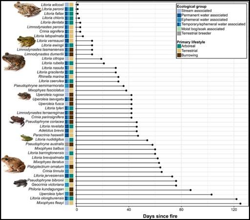
frogs within the fire footprint may have persisted in patches of unburnt habitat of various sizes, which are common, particularly in shelter, wetter microhabitats where fires tend to burn at lower intensity (Rowley, 2020). The method FrogID professionals used in the report is evidence of short-term persistence and attempted breeding activity, but this approach cannot inform estimates of breeding success or recruitment, which is necessary for population dynamics and other areas such as the frog’s environment (e.g., vegetation, water bodies, connectivity). Subtle impacts such as increasing vulnerability to extinction from further effects of the burnt areas are also not immediately evident from the study.
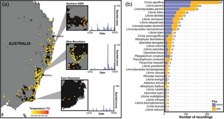 Figure 2. Map of the study area, showing the National Indicative Aggregated Fire Extent Dataset (black), and the temperature of the DEA hotspots with FrogID records (both pre- and postfire) (Dr Jodi Rowley, 2020).
Jodi Rowley, 2020).
Figure 2. Map of the study area, showing the National Indicative Aggregated Fire Extent Dataset (black), and the temperature of the DEA hotspots with FrogID records (both pre- and postfire) (Dr Jodi Rowley, 2020).
Jodi Rowley, 2020).
The Journal of Science Extension Research – Vol. 2, 2023 education.nsw.edu.au 103
Scientific research question
Has the distribution of frog species stayed the same before and after the 2019-2020 bush fires across NSW? If so, why have specific species had dramatic increases or decreases in distribution.
Scientific hypothesis
Following the Currowan bushfires, the distribution of frog species was negatively affected, resulting in a decline after the fires.
Null hypothesis: There is no difference in the distribution of frog species across coastal NSW since the 2019-2020 Currowan wildfires.
Alternate: There is a difference in the distribution of frog species across coastal NSW since the 2019-2020 Currowan wildfires.
Methodology Aim
The aim of the primary and secondary data gathering, and subsequent investigation was to determine if there was a difference in the frog species distribution before and after the megafires in 2019-2020. The use of a ‘blended’ application of investigative technologies is used for validity of results and accurate evidenced based conclusions. Both include quantitative and qualitative data.
Note: The results, discussion and conclusions are drawn extensively from the secondary investigation of data.
Primary investigation method:
Three burnt and three non-burnt frog habitats in Conjola and Milton, NSW were
identified. Sites contained similar sized dams and habitats. Frog calls were recorded between 6:00pm and 8:30pm for one minute using the FrogID app (Museum, 2017) at each site. Potential frog species were identified on the app by comparing pre-recorded calls and submitted to Sydney Museum for clarification. Data collection was repeated in a random order for three nights in April 2022. The temperature, date, time, weather, and number of potential species were recorded at each site. Recordings were analysed and confirmed by Sydney Museum. As seen in Table 1, the identified species at each location was tabulated and compared.
Secondary data investigation:
All of NSW citizen science frog identification was obtained from the FrogID data (Museum, 2017) from 14th November 2017 to 15th July 2022. This data is considered co-owned due to containing this author’s primary sourced data. The FrogID data is sourced from citizens across Australia sending in their recordings of frog calls (recorded on mobile phone via the FrogID app), which are then identified by experts at the museum and entered in the national frog data base. The NSW data set contained 59,694 results including qualitative and quantitative data on recorder ID, type of water body, longitude/latitude, species name, time, and date of recording. Data was sorted by dates before (10th Nov 2017 – 30th June 2019), during (1st July 2019 – 29th Feb 2020), and after (1st Mar 2020 – 9th Nov 2020) the 2019-2020 NSW megafires. A summary of the data set can be found in the Table 2 in the results. The data was graphed showing number of incidences of each species comparing before, during and after the
The Journal of Science Extension Research – Vol. 2, 2023 education.nsw.edu.au 104
fires. From these graphs four species were visually selected due to sharp decreases or increases in numbers for closer investigation. Information was gathered on whether the species was a tree or ground frog, breeding periods and other relevant information using the FrogID information website (Museum, 2017). Using longitude and latitude, the four species distributions were mapped

on a NSW map using a mapping program (Maptive, n.d.), comparing the three periods.
Results
The results follow the order of methodology, including primary data collecting and secondary data assortment.
Table 1. Results of the primary investigation. The brown colour indicates fire affectected and the blue colour indicates non-fire affected area. The average number of species in nonburnt species (A=2.8) is higher than burnt areas (A=2.5). This data was limited due to the time of collection not being preferable in that is was before most species breeding season (meaning the calls were scarce).
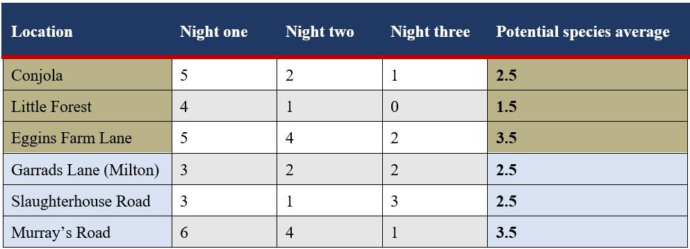 Primary investigation results:
The Journal of Science Extension Research – Vol. 2, 2023 education.nsw.edu.au 105
Figure 4. Graphical representation of the primary results without manipulation.
Figure 5. detailed map
local area indicates the extent of the severity of the bushfires on vegetation with accuracy of 15 metres (government, 2022). The pick dots represent the areas that were burnt and blue for unburnt. Each burnt site was ‘very highly’ affected, as seen on the map key.
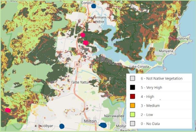
Secondary investigation results:
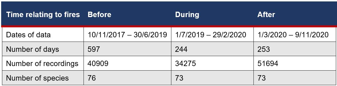
Table 2. The relevant periods in which data was organised. 3 species have not been detected after the fires. The number of recordings is also larger ‘before’ resulting in a possible skew effect of results.
Figure 6. Data of before, during and after the fires of less prevalent species. It can be observed that some species were not recorded calling after the fires, and some species spiked during the fire and most species presence depreciated after the fires.
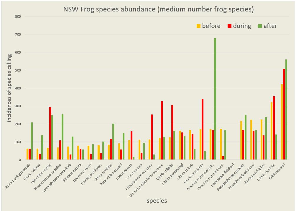
Figure 7. Data of before, during and after the fires of the species that were slightly more prevalent. Disparate results can be compared Figure 4. For instance, many of the species’ incidences dramatically increased following the fires.
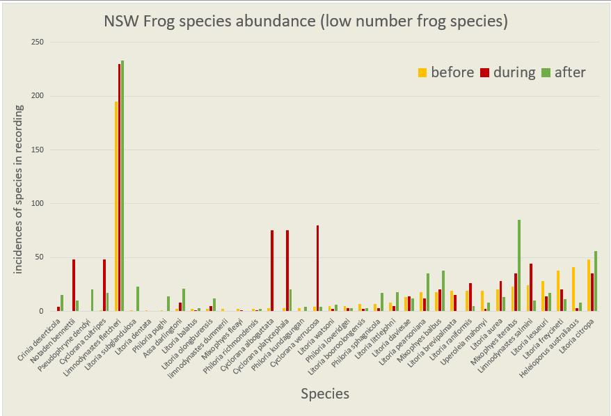 of
of
The Journal of Science Extension Research – Vol. 2, 2023 education.nsw.edu.au 106
Figure 8. Data of species before, during and after the fires of the species with calls that were commonly recorded. The trends include some species increased before the fires and some decreased. The blue circled species had dramatic increases or decreases in calling. The species will be investigated in depth in the discussion.
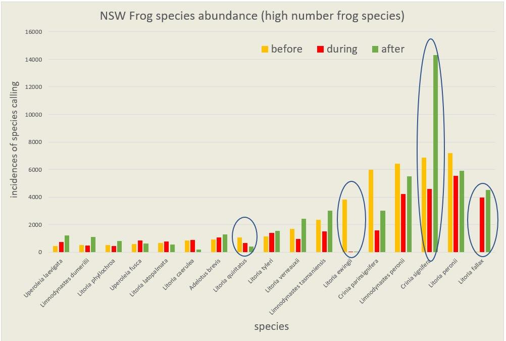
Figures 13 and 14. indicate the location of species Litora ewingii before and after the fires (there is no during due to the species not being calling during this period. Clearly, the species has decreased dramatically, along the coastline, including fire-affected areas. Figure 15. locations of where the species is found (FrogID, 2018).
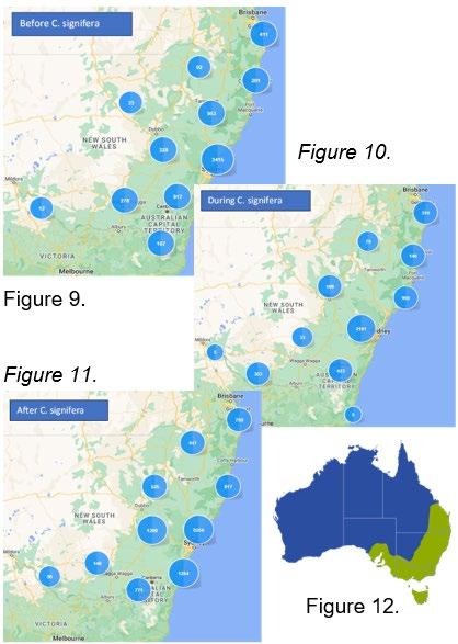
Figure 9., 10. and 11. indicate the number of Crinia signifera calls before during and after the fires on a map of coastal NSW. The species has nearly doubled its prevalence after the fires, including fire affected areas. Figure 12. locations where the species
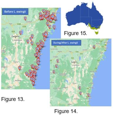
The Journal of Science Extension Research – Vol. 2, 2023 education.nsw.edu.au 107
Figures 16., 17. and 18. Indicate the locations species Litora quiritatus which population numbers also declined throughout each time period. Figure 19. indicates where the species is found a small part of NSW which was heavily fire affected (FrogID, 2018).

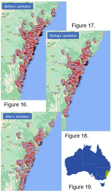
Figures 20., 21. and 22. Indicates the locations of species Litoria fallax. It can be observed that the species presence was sparring before the fires and increased both during and after the fires. Figure 23. indicates the location of where the species was found which is predominantly in Queensland but also throughout the fire zone (FrogID, 2018).
The results show considerably variation in frog population before, during and after the fires. Most frog species are coastal and were therefore within the fire zone (Figure 1). Of the 76 species, 38 species increased in number, 28 species decreased, and 10 species had no notable change before and after the fires. Therefore 50% of the frog species increased in numbers after the fires.
The Journal of Science Extension Research – Vol. 2, 2023 education.nsw.edu.au 108
Discussion
Formation of argument/explanation of results
Primary investigation: The results obtained from the primary investigation offered a small level of evidence in favouring the alternate hypothesis. The average number of potential species in non-burnt areas was 0.3>burnt areas. Explanations towards this result could include: a loss of vegetation in fire affected habitats, frog species struggling to rejuvenate, reduction in available insects/food sources. Alternatively, when considering the minor difference in results, explanations for the null hypothesis could potentially include loss of predatory species in fire-affected areas, although this is unlikely to influence the long-term results (as migration of these species occurs in the short term once vegetation begins to rejuvenate), but rather would have an affect on the species ability to recover short-term. Furthermore, there is sufficient evidence collected from FrogID scientists that some species were detected at sites that continuously burnt at a high temperature, meaning many species and possibly their spawn would have been able to evade the fire/heat in moist environments. (Dr Jodi Rowley, 2020).
Secondary investigation: Overall, the occurrences of frog species did not decrease, but rather increased post-fire. Although, during the fire period, the occurrences of some species dramatically declined. These results would infer that species were able to recover long-term and a combination of factors lead to the most species declines amidst the ‘during’ period. This period ranged for 7 months
between 2019 and 2020, in which weather conditions were humid and continuous bushfires occurred. An article composed by the Australian Bureau of Meteorology, stated in 2019 “total rainfall for New South Wales was the lowest on record, at 55% below average; well below the previous driest year of 1944” (Meteorology, 2020). It also explains that 2019 was the hottest year on record for NSW, surpassing that of the previous record year in 2018 (Meteorology, 2020). These conditions had tremendous impacts on frog species survival in addition to the Currawong fires. The dry and hot weather forced species to compete for sparring habitat and resources or destroyed (dried up) their habitat altogether. With these presumptions, conclusions can be drawn that species distribution increased throughout the post-fire period (7 months in 2020) predominately due to the contrasting change in weather conditions. The Bureau of Mereology described NSW weather in 2020 as “the coolest and wettest for since 2012” (Meteology, 2021). In attempt to extend the investigation of results, the following species were chosen for their outlying increases or decreases in recording for an in-depth analysis:
As evidenced in the results, species Litoria ewingii’s (seen in Figure 24) calling dramatically decreased post-fire, from an estimated 3950 to 10s post-fire. The
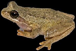 Litoria ewingii:
Figure 24
Litoria ewingii:
Figure 24
The Journal of Science Extension Research – Vol. 2, 2023 education.nsw.edu.au 109
species is more common in South Australia but is still found in NSW fire zone. The species is a hylidae (tree frog), calls throughout the year, has a long breeding season (Jun-Nov). It lays its spawn underneath vegetation in temporary or permanent water bodies (FrogID, 2018). Treefrogs would perish in fires as they are isolated from water bodies and the fires crowned. Eggs in small pools and only protected by vegetation would also be vulnerable to fire. Both situations may have negatively impacted the species.


Litoria quiritatus:
Likewise, species Litoria quiritatus (seen in Figure 25) recordings decreased from an estimated 1000 to 300. The species is located throughout the fire zone along the coastal regions of NSW. Litoria quiritatus is also a hylidae and has a long breeding time (throughout Spring and Summer) although only following heavy rain. The species also lays in water bodies (FrogID, 2018). FrogID scientists collected data which indicated the species continued to call at sights that continuously burnt at a high temperature (290-530 degrees C) (Dr Jodi Rowley, 2020), contrary to these results.
Disparately, species Crinia signifera (seen in Figure 26) recordings dramatically doubled from an estimated 6900 pre-fire to 14400 post-fire. Located throughout most of NSW, heavy throughout the fire zone. The species is a common myobatrachidae (Aus. ground frog), has a long breeding season (FebNov), lays spawn in a variety of water bodies and is very small (3cm max length) (FrogID, 2018). A myobatrachidae species may have found refugee in water bodies in the fires (identified by Dr Rowley, 2020). On inspection of my property, which was severally affected by fires and one of the test sights, unusually large numbers of frogs were observed in the dam a day after the fire had passed (Dr Kneeshaw, personal observations). This species spawns in permanent water bodies which are unlikely to be affected by the fire. Existing tadpoles would therefore be able to repopulate an area.
Litonia fallax:
Likewise, species Litonia fallax (seen in Figure 27) recordings increased dramatically from in the 10s to 4500 postfire. The species is a hylidae, has a short breeding time (Sep-Dec) although is
Figure 25
Crinia signifera:
Figure 26
Figure 27
The Journal of Science Extension Research – Vol. 2, 2023 education.nsw.edu.au 110
known to breed anytime in the year and lays spawn in permanent water bodies. This frogs adaptation to breed at any time may have given this species an advantage with the post-fire rainfall.
Declines in species could also be attributed to a decline in food availability as insects were not able to escape fires. It could be speculated that increase in some species may be due to a lack of competition, predators and/or adaptive breeding in wetter conditions. C. signifera a ground frog, become sexually mature faster than tree frogs (FrogID, 2018).
Female C. signifera can become sexually mature 1 year after metamorphosing (Lauck, 2004). Speed in sexual maturity may have benefited this frog’s recovery and now dominance across NSW.
Female tree frogs can take over 3 years to sexually mature (Government, 2021). If adults were lost due to fires, surviving tadpoles in these species may take 3-4 years to recover as breeding populations.
Evaluation of data-analysis
Overall, with access to the secondary data base, more conclusions were able to be drawn. Ultimately both the null and alternate hypothesis was satisfied and sufficiently evidenced using both primary secondary, therefore data-analysis was strong.
Primary data: Benefits and Limitations
Benefits of the primary data-analysis include that all recordings are verified by professionals from FrogID (FrogID, 2018), data was collected 3 times and the data allowing for statistical analysis that somewhat satisfied answering the hypothesis. Limitations included the time of year was not optimal for frog calling, and the data collection process was not
repeated throughout the year, leading to decreased validity of analysis.
Secondary data: Benefits and Limitations
The validity and reliably of the FrogID data base provided my investigation with a well evidenced report. Limitations include the numbers of recordings being different in each time period and more members recording more often than others, both resulting in potential skewing of results.
Suggestions for further directions
As established there is not much data or evaluable information regarding the longterm recovery of frog species, and the effects of mega-fires on threatened species, meaning this reports hypothesis or area of interest could potentially provide scientists with authentic conclusions and/or ideas. These ideas can also be used for future fire recovery predictions. The report also attempts to decipher why some common species increased or decreased in numbers, although trends continue to appear vague. Once these conclusions are drawn, scientists can implement mechanisms to support the conservation of species that are declining.
Conclusion
The primary investigation offered the unreliable conclusion that there is a higher number of species in non-fire Currawong affected areas around the local area. Whereas the secondary investigation, which was considerably more reliable, evidenced that the number of species was generally low across all species during the fires, and dramatically increased after the fires. Reasoning behind these results were assessed to be
The Journal of Science Extension Research – Vol. 2, 2023 education.nsw.edu.au 111
due to contrasting weather conditions (being hot and dry ‘during’ and cold and wet ‘after’). Other subtle impacts included some species taking advantage of the wet weather post-fire resulting in a fluctuation of offspring throughout the whole year, potential loss of predators and disparate environments. Long-term data (3-5 years following fires) may be required to observe if populations to recover as tadpoles laid during the fires become mature.
References
BBCnews, 2020. Australia fires: A visual guide to the bushfire crisis, s.l.: s.n.
Brendan A.Wintle, S. J. C. W., 2020. After the Megafires: What next for Australian Wildlife?. Trends in Ecology and Evolution, p. 11.
Dederer, A., 2020. AUSTRALIA’S 20192020 BUSHFIRES: THE WILDLIFE TOLL, s.l.: s.n.
Dr Jodi Rowley, D. C. C. D. W. C., 2020. Frogs surviving the flames. FrogID, p. 4. FrogID, 2018. Explore Frog Profiles. [Online] Available at: https://www.frogid.net.au/frogs [Accessed 2022].
Garry Daly, P. C., 2011. Monitoring populations of Health Frog Litoria littlejohni in the shoalhaven region on the South Coast of NSW. AGRIS, p. 2.
Government, A., 2021. Species Profile and Threats Database. [Online] Available at: http://www.environment.gov.au/cgibin/sprat/public/publicspecies.pl?taxon_id =25959 [Accessed 2022].
government, N., 2022. Google Earth Engine Burnt Area Map (GEEBAM)
[Online] Available at: https://datasets.seed.nsw.gov.au/dataset/ google-earth-engine-burnt-area-mapgeebam [Accessed 2022].
Lauck, B., 2004. Life history of the frog Crinia signifera in Tasmania, Australia. Australian Journal of Zoology, 53(1), pp. 21-27.
Lindenmayor, D., 2001. Use of farm dams as frog habitat in an Australian agricultural landscape: factors affecting species richness and distribution. Biological Conversation, p. 5.
Maptive, n.d. Mapping Software for every Professional. [Online] Available at: https://www.maptive.com/ [Accessed 2022].
Meteology, A. B. o., 2021. New South Wales in autumn 2020: wet and cool [Online] Available at:
http://www.bom.gov.au/climate/current/se ason/nsw/archive/202005.summary.shtml #:~:text=Autumn%202020%20in%20New %20South,the%20north%20and%20sout h%20coasts [Accessed 2022].
Meteorology, A. B. o., 2020. New South Wales in 2019: record warm and record dry. [Online] Available at: http://www.bom.gov.au/climate/current/an nual/nsw/archive/2019.summary.shtml [Accessed 2022].
Museum, A., 2017. Australia’s frogs need your help. [Online] Available at: https://www.frogid.net.au/
Museum, A., 2017. Explore frog profiles. [Online] Available at: https://www.frogid.net.au/frogs
Museum, A., 2020. Australia's Native Frogs. [Online] Available at:
The Journal of Science Extension Research – Vol. 2, 2023 education.nsw.edu.au 112
https://australian.museum/learn/animals/fr ogs/#:~:text=Frogs%20are%20the%20onl y%20remaining,both%20terrestrial%20an d%20aquatic%20environments.
[Accessed 2022].
Museum, S., 2017. Explore FrogID records. [Online] Available at: https://www.frogid.net.au/explore
[Accessed July 2022].
Rowley, J. R. L., 2020. Widespread shortterm persistence of frog species after the 2019-2020 bushfires in eastern australia revealed by citizen science. FrogID.
The Journal of Science Extension Research – Vol. 2, 2023 education.nsw.edu.au 113
The Effect of Shrub Layer Composition on Bird Abundance and Species Richness in Revegetation plantings in Hilltops
NSW
Hannah Southwell Boorowa Central School
The intensification of agriculture in the Hilltops region in NSW, has led to the decline in bird populations. Revegetation plantings are one common strategy to deal with this crisis. This study examines how the composition of the shrub layer within revegetation plantings affects species richness and abundance of birds. Vegetation and bird surveys were conducted at 10 revegetation plantings on farms in the Hilltops local government area. The hypothesis that plantings with ahigh shrub density would also have high bird abundance and species richness, was rejected. However, other trends were observed in the data; from these trends, it can be concluded that revegetation plantings in agricultural regions are an indispensable source of habitat for birds and the use of them is highly valuable to conservation efforts. The value of these plantings to birds increases with increasing vegetation density, and more specifically, tree density. It is therefore important to maintain existing areas of established and mature native trees for the benefit of birds.
Literature Review
The Action Plan for Australian Birds 2020 recognises 1 in 6 Australian bird species as nationally threatened in accordance with the IUCN Red List criteria. (Birdlife International,2022). One of the major factors contributing to this is a loss of habitat resulting from the clearing of native vegetation in agricultural areas (Stevens, 2001). Within the Hilltops Local Government area, over 80% of the native vegetation has been cleared for agriculture. (Reid, 2000; NSW National Parks and Wildlife Service, 2002) with the National Parks and Wildlife Service describing the state of the vegetation in the Hilltops region as ‘perilous’. (NSW National Parks and Wildlife Service, 2002, p. v) One of the most common restoration efforts in the Hilltops area is farm revegetation plantings. They can be
seen on properties throughout the region and include areas of managed remnant vegetation as well as planted natives. Research has been conducted to determine the suitability of revegetation plantings for bird habitat. A key focus of this research is the comparative value of remnant native vegetation and revegetation plantings to birds. Cunningham et al. found that “remnant native vegetation on farms is critical for many declining bird species” (Cunningham et al.,2008, p. 750) and that whilst farm plantings may offset the loss of remnant vegetation for some species, overall the existing native vegetation is more important for species increase (Cunningham et al., 2008) .However, whilst it is clear that revegetation plantings on farms are not an adequate substitute for remnant vegetation, further research indicates that in heavily modified
The Journal of Science Extension Research – Vol. 2, 2023 education.nsw.edu.au 114
agricultural landscapes “plantings in general can provide habitat for many species of birds” (Munro et.al., 2011, p. 223). This is further supported by surveys conducted by Greening Australia researchers at a farm in the Hilltops region. Surveys of the native vegetation and birds were conducted several times between 1980 and 2019. They found that as the areas of native vegetation increase due to revegetation, so did the number of birds observed in the surveys. (Hosking and Thackway, 2019). This confirms the importance of revegetation plantings as a strategy for the conservation of bird species in agricultural landscapes. Whilst revegetation plantings are beneficial to birds overall, many factors affect the success of a revegetation planting as bird habitat. Haslem et. al. (2021) found strong evidence that the human management of revegetation plantings strongly influences its suitability as a bird habitat. It is, therefore, crucial that land managers have a well developed understanding of how to best manage factors of plantings that benefit bird species. One such factor is the structure of a revegetation planting, multiple studies (Lindenmayer et al., 2018: Munroet. al., 2011) have found a correlation between the structure of a planting and its suitability for bird habitat. Lindenmayer et al. (2018) found, after conducting bird surveys at 61 sites, that an increase in both the size of a remnant woodland and the amount of understorey within it will positively affect birds. However, they also discovered that increasing the amount of understorey has a negative effect on Noisy Miners (Manorina melanocephala). As Noisy miners are aggressive, their presence often leads to a decrease in other bird species. Munroet. al., 2011 focused on bird species richness and composition in
four different environments: remnant forest, cleared agricultural land, woodlot plantings (containing only native trees) and ecological plantings (containing a wide variety of trees, shrubs and understory plants). The ecological plantings were found to have a larger diversity of bird species than the woodlot plantings (Munro et. al., 2011).
Additionally, birds found in the ecological plantings were “shrub-associated birds” (Munro et. al., 2011, p. 223) compared to the “generalist bird species” (Munro et. al., 2011, p. 223) found in the woodlot plantings.
In relation to the specific types of birds benefitted by revegetation plantings; Lindenmayer et. al. (2018) examined the changes to bird species in old-growth woodland, regrowth woodland and restoration plantings over 13 years. They observed an overall increase in smallbodied species of birds particularly in restoration plantings (Lindenmayer et. al., 2018). A substantial amount of research has demonstrated the extensive value of revegetation plantings for bird abundance and diversity. The characteristics of plantings that benefit birds are still being investigated. However, the general theme of the literature suggests that having more ‘shrub’ species in the understorey of a revegetation planting may lead to increased bird diversity. Although further research is clearly required to confirm these findings.
The Journal of Science Extension Research – Vol. 2, 2023 education.nsw.edu.au 115
Scientific Research Question
How does the composition of the shrub layer in revegetation plantings affect the abundance and species richness of birds in Hilltops NSW?
Scientific Hypothesis
Within revegetation plantings, the density of the shrub layer will have a strong positive correlation with bird abundance and species richness. The literature suggests that a greater percentage of the population will be small-bodied birds because these species rely on native plants for food and shelter from predators
Methodology
Plantings
10 revegetation plantings were located within the Hilltops local government area. To ensure validity, a revegetation planting was defined as; an area of less than 2 hectares consisting primarily of native vegetation, that includes some tree species and has been managed (planted, fenced off or protected in some way) by the land owner or by an organisation on the land owner’s behalf. The area may include existing woodland remnants but is isolated from large areas of scrub. All sites were a minimum distance of 100m from all other sites to ensure independent and valid results.
Vegetation Data
For each revegetation planting two researchers collaborated to collect the vegetation data. The length and width of the planting was measured using a trundle wheel and Google maps. This was practical and accurate to the nearest metre. Then the number of alive and dead shrubs, trees and thickets inside the planting were counted. A shrub was defined as a plant that is between 1 and 3 m tall and at least 50cm wide (with fairly dense foliage). Any plant taller than a shrub was recorded as a tree. A thicket was defined as an area of shrubs that are growing so close together that their individual stems cannot be counted and their leaves form a single canopy. A
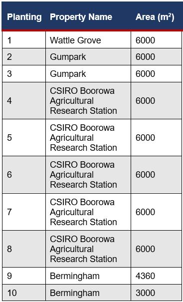 Table 1- The revegetation plantings used in this experiment.
The Journal of Science Extension Research – Vol. 2, 2023 education.nsw.edu.au 116
horticulturalist was consulted to create a list of the most common native plants found in each planting and any introduced plant species.
Bird Survey
At each site a researcher used the Birdata app to record a survey using the 20 minute search method (sensu Loyn, 1986). This method was chosen because of its validity to the objectives of the study. Any bird species that were seen or heard in the 20 minute period were recorded directly into Birdata while in the field. Birds that flew over the area were only counted if they were obviously using the area (eg. Birds of prey, hunting in the planting). Bird’s that could not be identified were listed as unknown species so as not to affect the accuracy. All surveys were conducted during the day and the permission of the landowner was obtained before entering the property. Over the next 2months, 4 surveys were recorded at each site. Surveys were not conducted in high wind, rain or fog as these conditions can affect results (Field et. al, 2002). A safety induction was completed at each property to ensure the safety of the researchers.
Analysis
Following the collection of vegetation data, shrubs per hectare, trees per hectare and plants per hectare. The results of the experiment were analysed by creating scatter plot graphs and calculating the Pearson’s Correlation coefficient. This allowed the correlations between variables to be clearly seen. The Birdata (Birdlife, 2022) website was used to create a polygon of the Hilltops area. The website contained all of the data from bird observations submitted to Birdlife Australia, which is a highly reliable
source. All species were then classified into the following categories: water birds, ground birds, birds of prey, small-bodied birds and large-bodied birds. This was compared to the data from the experiment using a Chi-squared test.
Results
Figure 1- Graph representing the correlation between the average number of individual birds observed in each planting (abundance) and the number of shrubs per hectare. There is a very weak linear correlation between the two variables.
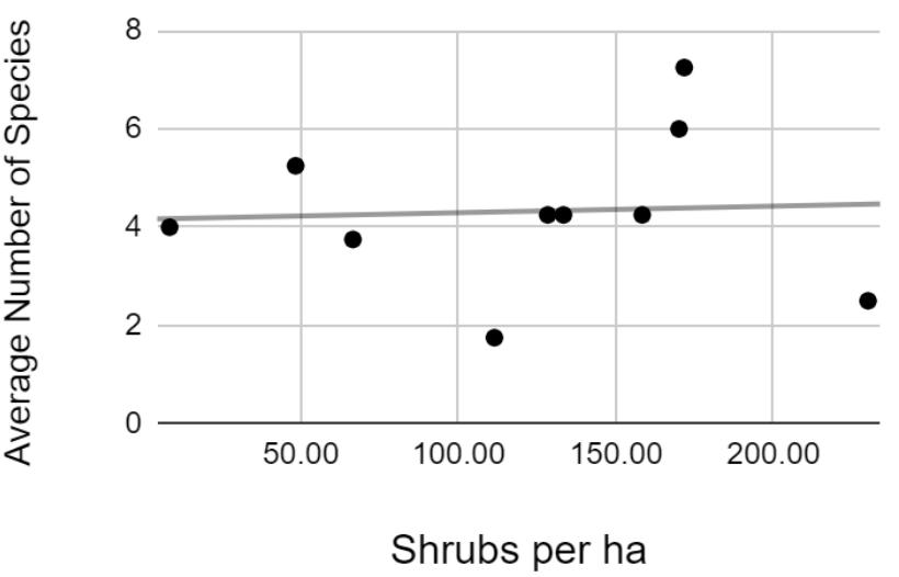
Figure 2- Graph representing the correlation between the average number of bird species observed in each planting (diversity) and the number of shrubs per hectare. There is a very weak linear correlation between the two variables.
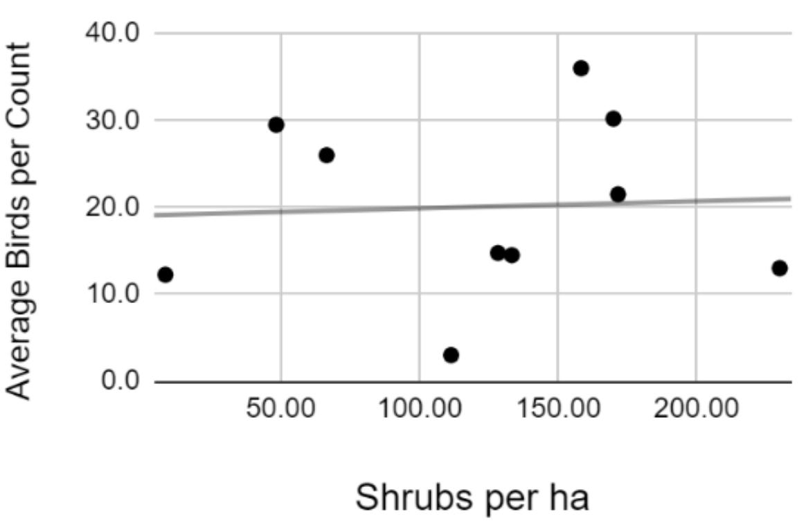
The Journal of Science Extension Research – Vol. 2, 2023 education.nsw.edu.au 117
Figure 3- Graph showing the correlation between the percentage of observations that were small-bodied bird species and the number of shrubs per hectare. There is a very weak linear correlation between the two variables.
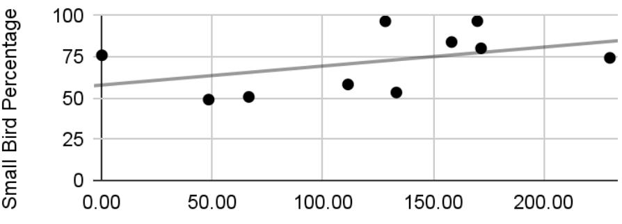
Callistemons, grevilleas and hakeas were also counted in smaller numbers.
Plantings located closer together did not necessarily contain similar vegetation, demonstrating the effect of human management.
Table 2-The statistical results of the experiment, all of the results are very low, indicating that there is only a very weak correlation between variable
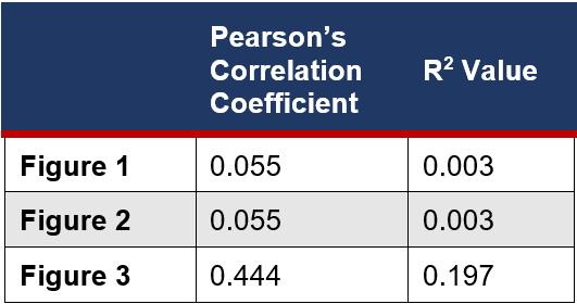
Discussion
This experiment examined the effect of shrub density on bird abundance and species richness in revegetation plantings in the agricultural region of Hilltops, NSW.
The revegetation plantings (appendix 1) chosen represented a wide variety of different planting structures, although some were similar. Planting 6 had the highest total number of plants and also had a comparatively high number of dead trees and shrubs. Only a few of the plantings contained thickets, however those that did tended to have a high number of them. These included plantings3, 6, 7 and 10. Planting 4 consisted of eucalypt trees with only 5 shrubs counted. The most common species across all plantings were eucalyptus and acacia species.
The highest number of birds was observed in planting 7 whilst planting 2 displayed a very low abundance of birds (appendix 2). A very similar number of birds was found in plantings1 and 8. No water birds were seen during the surveys and only 2 ground birds were observed. 3 birds of prey were seen and all other birds were in the small-bodied bird or large-bodied bird categories. The highest number of species observed in one planting over the 4 surveys was 18 in planting 3 (appendix 2). Plantings 2 and 7 both had the lowest species richness of 7 species. Planting 8 had the highest percentage of small-bodied bird species and also the lowest percentage of largebodied bird species.
When bird abundance and species richness were graphed against shrubs per hectare, the correlation was positive but extremely low (Figures 2 and 3). Interestingly the correlation coefficient was the same for both graphs. This may indicate a relationship between bird abundance and species richness. The correlation coefficient for the percentage of small birds and the abundance and species richness of small birds was higher, indicating as lightly stronger correlation, although still not significant. Accordingly, the null hypothesis must be accepted and the alternate hypothesis rejected. It is therefore concluded that there is no statistically significant difference between the density of shrubs in a revegetation planting and the diversity and abundance of birds
The Journal of Science Extension Research – Vol. 2, 2023 education.nsw.edu.au 118
observed there. This contradicts the common findings in the literature.
Limitations
The most significant source of error in this investigation was in the definition and classification of both plants and birds. For this experiment, shrubs were defined as ‘a plant that is between 1 and 3 m tall and at least 50cm wide (with fairly dense foliage)”. Any plant taller than a shrub was recorded as a tree. The purpose of classifying the vegetation in this way was to isolate the different structures within revegetation plantings in order to relate patterns in bird observations to one specific type of plant. However, identifying a plant as either a shrub or a tree was still dependent on the discretion of the observer. This may have impacted the accuracy of this investigation. Furthermore, ‘trees’ encompassed both mature eucalypts and younger trees which have very different ecological functions. In future experiments, different methods of quantifying vegetation density should be explored. For example a habitat complexity score (Tay,2019).
Birds were also classified for this investigation. This was done based roughly on their size, taxonomic group and ecological niche. However this investigation would be more valid if the birds had been grouped using a more systematic approach. For example, if all birds with a wingspan less than 20cm were listed as small-bodied birds. Finally, this investigation would be more reliable if more bird surveys were conducted, although this would be less practical and achievable.
Other Findings
Whilst no correlation was observed between shrub cover and bird abundance and species richness, there were other patterns in the data collected. As can be seen in Figure 5, there was a high correlation between the number of trees per hectare and the abundance of smallbodied birds and an even higher correlation between the number of plants per hectare (including all plants counted) and small-bodied birds. This correlation suggests that tree density and total vegetation is more important for bird species than shrub density.
In this experiment, for a plant to be defined as a ‘tree’ it had to be taller than 3m and therefore well established. The correlation between increased trees per hectare and increased bird observations suggests there may be a connection
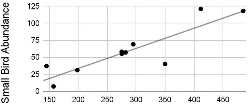
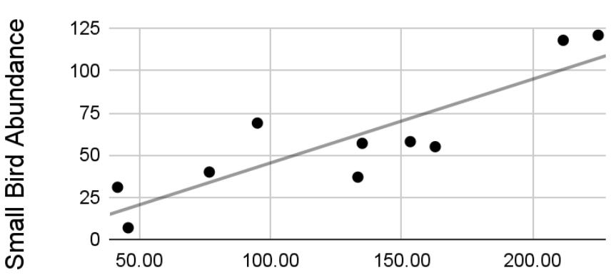 Figure 5- Graph showing a high positive correlation between abundance of smallbodied birds and trees per hectare. This relationship has an R2 value of 0.758.
Figure 6-graph showing a very high positive correlation between abundance of small bodied birds and plants per hectare. This relationship has an R2 value of 0.771.
Figure 5- Graph showing a high positive correlation between abundance of smallbodied birds and trees per hectare. This relationship has an R2 value of 0.758.
Figure 6-graph showing a very high positive correlation between abundance of small bodied birds and plants per hectare. This relationship has an R2 value of 0.771.
The Journal of Science Extension Research – Vol. 2, 2023 education.nsw.edu.au 119
between the age of a planting and bird diversity and abundance. This could confirm the findings of Cunningham et. al.(2008), by supporting the idea that remnant vegetation is more valuable as bird habitat than revegetation plantings.
Further conclusions can be drawn using the Hilltops polygon obtained from Birdlife Australia data. On average, 38.4% of individual birds observed in the Hilltops area were small-bodied birds compared to between 52-97% small-bodied birds observed in this experiment. Additionally, 28.4% of species in the Hilltops polygon were small-bodied birds compared to between 40-85% in the experiment. Chi squared tests were performed to compare the ratio of small-bodied birds to largebodied birds in the Hilltops polygon and the data from this experiment to determine if this difference is statistically significant (appendix 3). This was done for each planting and for both abundance and species richness data. Every planting showed a p value of significantly < 0.05 for both tests with the exception of the abundance test for planting 5 which had a p value of 0.13. This means the ratio of small to medium birds and bird species is significantly different in agricultural revegetation plantings compared to the average ratio found in the Hilltops region. This suggests revegetation plantings are hugely beneficial to small-bodied bird species.
The most common species observed throughout the surveys was the Superb Fairy-wren (Malurus cyaneus) with 258 counted (appendix 4). They made up 32.09% of birds sighted in the surveys compared to 3.4% in the Hilltops region. This indicates that revegetation plantings are valuable habitat for the Superb Fairywren (Malurus cyaneus). The second
most common species was the Yellowrumped Thornbill (Acanthiza chrysorrhoa) followed by the Crested Pigeon (Ocyphaps lophotes)and then the Yellow Thornbill (Acanthiza nana). The high number of crested pigeon sightings is suspected to be due to the repeated sighting of a large flock in the same planting. The presence of 3 small-bodied bird species in the 4 most common species observed further affirms the benefits of revegetation plantings for small birds. Further research could involve developing a better understanding of the value of revegetation planting to these species. Most other species were present in insignificant ratios compared to the polygon.
Conclusion
The results of this experiment refute the hypothesis that revegetation plantings with a higher density of shrubs also support a greater bird abundance and species richness. The correlation between shrub density and both bird abundance and species richness was positive but very weak (R2= 0.003 for both). The correlation between the percentage of birds that were smallbodied and the shrub density was slightly higher (R2= 0.197) but still insignificant. There were limitations to the accuracy of this study including the methods of classifying both birds and vegetation. In future research, alternate methods of measuring vegetation type should be employed. Whilst the hypothesis was rejected, other trends in the results suggest that the vegetation within a revegetation planting is important for bird abundance and species richness. A strong correlation was found between bird abundance and tree density and an even stronger correlation was present between
The Journal of Science Extension Research – Vol. 2, 2023 education.nsw.edu.au 120
bird abundance and plant density. From this it can be concluded that an increase in overall vegetation density does lead to an increase in bird abundance and species richness. Comparing the results of this study to the data from Birdata allows further conclusions to be drawn. As shown by Chi squared tests, there is a statistically significant difference between abundance and species richness in revegetation plantings and the average abundance and species richness in the Hilltops region. Therefore, revegetation plantings are important for birds, particularly small-bodied species such as the Superb Fairy-wren (Malurus cyaneus). Further research is required to establish the reason that plantings are so beneficial to small-bodied birds. Further study in this area of research could include focusing on the plant species in revegetation plantings and the genera that compose plantings that are particularly suitable for bird habitat. Similar studies to this should also be conducted in regions that specialise in different sectors of the agricultural industry such as broad-acre cropping.
In conclusion, within the agriculturally intense region of Hilltops, NSW, revegetation plantings provide valuable habitat for birds. Whilst they cannot replace native vegetation cleared for agriculture, their implementation on farms can increase bird abundance and species richness. No link has been established between shrub density and bird abundance and species richness, although there is evidence to suggest that higher vegetation density supports greater bird abundance.
Acknowledgements
I would like to thank Eleanor Lang from the Australian National University for her advice regarding this study and for providing feedback on it. I would also like to thank Jayden Gunn from Birdlife Australia for his suggestions and assistance with the preliminary surveys. Also thanks to Dr Stuart Browne and the CSIRO Agricultural Research Station Boorowa, for allowing me to use their tree plantings. Finally, I wish to thank Craig Southwell for assisting in completing the vegetation surveys and providing knowledge of plant species.
Reference List
Birdlife International. (2022).The Action Plan forAustralian Birds 2020 reveals that one in sixare nationally threatened. BirdLife Data Zone. Retrieved13 July 2022,
fromhttp://datazone.birdlife.org/sowb/case study/the-action-plan-for-australian-birds2020-reveals-that-one-in-six-arenationally-threatened.
Cunningham, R., Lindenmayer, D., Crane, M., Michael, D., Macgregor, C., Montague-drake, R.,& Fischer, J. (2008). The Combined Effects of Remnant Vegetation and Tree Planting on Farmland Birds. Conservation Biology,22(3), 742-752.doi:
10.1111/j.1523-1739.2008.00924.x
Field, S., Tyre, A., & Possingham, H. (2002). Estimating bird species richness: How should repeat surveys be organized in time?. Austral Ecology,27(6), 624-629. doi:10.1046/j.1442-9993.2002.01223.x
Google Maps
(https://www.google.com/maps/@-
The Journal of Science Extension Research – Vol. 2, 2023 education.nsw.edu.au 121
34.571022,148.9207696,11z) was used for identifying and measuring plantings.
Haslem, A., Clarke, R., Holland, G., Radford, J., Stewart, A., & Bennett, A. (2021). Local management or wider context: What determines the value of farm revegetation plantings forbirds?.Journal Of Applied Ecology,58(11), 25522565.https://doi.org/10.1111/13652664.13988
Hosking, G., & Thackway, R. (2019). Birds, Biodiversity and Agricultural Land. Soils For Life. Retrieved 13 July 2022, fromhttps://soilsforlife.org.au/therelationship-of-habitat-and-biodiversityon-agricultural-land/.
Lindenmayer, D., Blanchard, W., Crane, M., Michael, D., & Florance, D. (2018). Size or quality.What matters in vegetation restoration for bird biodiversity in endangered temperate woodlands?.Austral Ecology,43(7), 798806. https://doi.org/10.1111/aec.12622
Lindenmayer, D., Lane, P., Westgate, M., Scheele, B., Foster, C., & Sato, C. et al. (2018). Tests of predictions associated with temporal changes in Australian bird populations. Biological Conservation,222, 212-221.
https://doi.org/10.1016/j.biocon.2018.04.0
Loyn, R. (1986). The 20 Minute Search –A Simple Method For Counting Forest Birds.Corella,10(2), 58-60. Retrieved fromhttps://absa.asn.au/corella_documen ts/the-20-minute-search-a-simplemethod-for-counting-forest-birds/
Munro, N., Fischer, J., Barrett, G., Wood, J., Leavesley, A., & Lindenmayer, D. (2011). Bird's Response to Revegetation of Different Structure and Floristics-Are “Restoration Plantings” Restoring Bird Communities?. Restoration Ecology,19(201), 223235.https://doi.org/10.1111/j.1526100x.2010.0070.x
NSW National Parks and Wildlife Service. (2002).The Native Vegetation of Boorowa Shire(p.2). Hurstville, NSW.https://www.environment.nsw.gov.a u/resources/nature/sbsnssscopeboorowa. pdf
Reid, J. (2000). Threatened and Declining Birds in The New South Wales SheepWheat Belt (p.1). Canberra: CSIRO.https://www.environment.nsw.gov .au/resources/nature/reportBirdsWheatSh eepBeltComplete.pdf.
Stevens, W. (2001). Declining Biodiversity and Unsustainable Agricultural Production-Common Cause, Common Solution?. Parliamentary Library.
https://www.aph.gov.au/About_Parliamen t/Parliamentary_Departments/Parliament ary_Library/pubs/rp/rp0102/02RP02.
Tay, Y. S. (2019). Bird species richness and abundance: The effects of structural attributes, habitat complexity and tree diameter. ANU Undergraduate Research Journal,9, 123–137. Retrieved from https://studentjournals.anu.edu.au/index.p hp/aurj/article/view/1
07
The Journal of Science Extension Research – Vol. 2, 2023 education.nsw.edu.au 122
Appendices
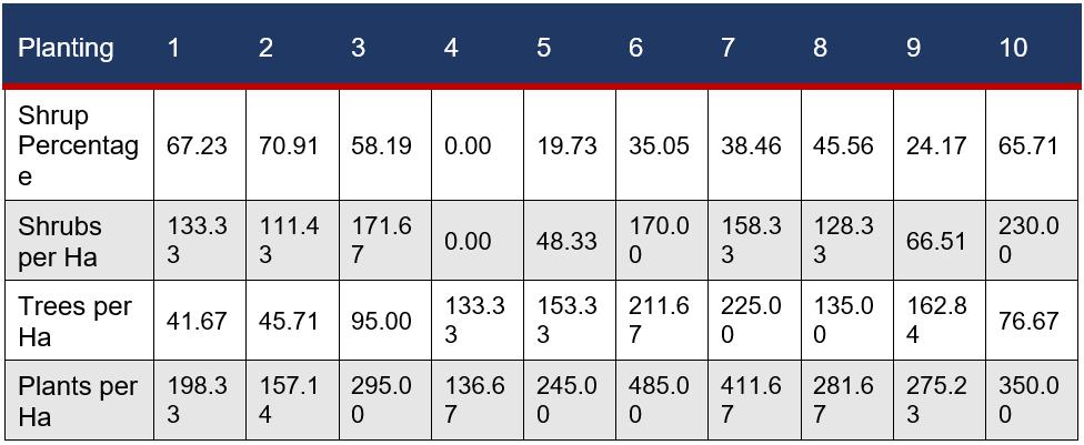
Appendix 1
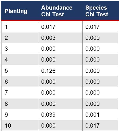
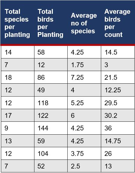
Appendix 2
Appendix 3
The Journal of Science Extension Research – Vol. 2, 2023 education.nsw.edu.au 123
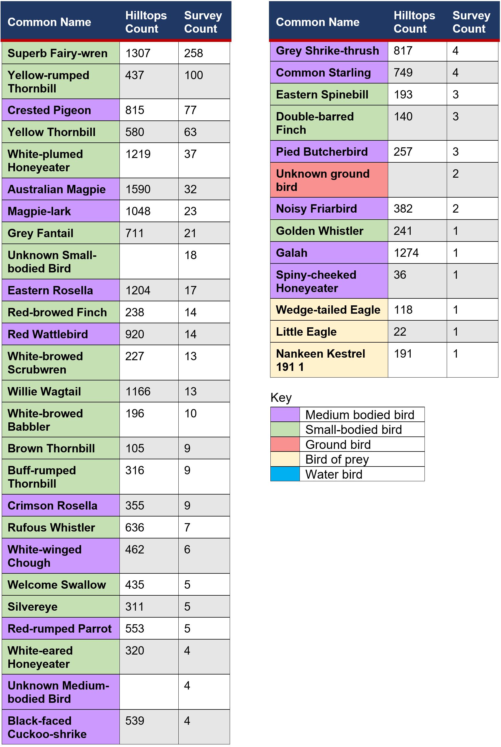
The Journal of Science Extension Research – Vol. 2, 2023 education.nsw.edu.au 124
Appendix 4
Investigating the effects of paragraphing and notetaking on memory recall and retention
Alexandra Vergel de Dios
Blacktown Girls High School
In this study the effect of paragraphing and note taking format on the recall of information was investigated. It extends the current research focused on textual format, typography, fonts and studying and their influence on readability, reading comprehension and observed retention of information. The retention of semantic information was tested in a short study session followed by a short-answer test to determine if a relationship between spaced text, and spaced notes resulted in higher rates of retention. The addition of note taking was added to determine whether there would be an observed effect in mean test scores between different formats of notes. After the data collection and initial data processing, planned contrasts were conducted to additionally test whether the presence of notes (combining both spaced and blocked notes) would also affect memory recall. The results showed that the presence of notes was significant and the interaction between notes and textual format, varied through paragraphing, was also significant.
Keywords: textual format, paragraphing, recall, retention, comprehension, reading, note taking
Literature review
Past studies (Larson and Picard, 2006; Gasser et al., 2005) have focused on typography and its effect on reading comprehension imposing different levels of textual formatting with an emphasis on text design, font type, interword and intraword spacing, text weighting and underlining. The general consensus appears to be that the formatting of texts has been observed to affect the comprehension and thus, the retention and recall of information. Other studies (Udomon et al., 2013; Santa et al., 1979) have addressed studying and note taking. However, few studies have related paragraphing to the retention and recall of textual information and incorporated the aspect of note taking.
Typography has been seen to have a notable effect on relative subjective duration in reading, attributing visual clarity to readability. Larson and Picard (2006) conducted a study testing the effects of poor typography and high quality typography on participants, with those who had the poor typography underestimating their reading time by 24 seconds, while good typography underestimated reading time by over 3 minutes on average. Poor typography was characterised by monospaced fonts (e.g. Courier New) with larger interword spaces, and good typography featured serif fonts (e.g. Times New Roman) with smaller interword spaces. While the study demonstrated the noticeable cognitive impact of typography and the elements of font symmetry and intraword spacing as
The Journal of Science Extension Research – Vol. 2, 2023 education.nsw.edu.au 125
contributing to visual readability, they did not attempt to explain the reason for the results.
Ljungdahl and Adler (2018) conducted a systematic review on relevant studies conducted with an emphasis on text design, focusing on studies that looked at how design and spacing contributes to reading accuracy, reading rate and reading comprehension. They chose studies that emphasised design rather than the content, and how readers were impacted. Their primary findings were that underlining and bolding words increased reading comprehension while other enhancements such as italics did not produce an effect on participants (Simard, 2008, as cited in Ljungdahl & Adler, 2018). In addition, a noticeable effect on legibility was seen through manipulation of fonts but not in font size, pixel height and font smoothing (Sheedy, 2005, as cited in Ljungdahl & Adler, 2018). This systematic review was useful in the development of the method for the current study and places a similar focus on how text format affects students’ learning outcomes. However, in contrast, this study does not consider how paragraphing and note taking affects the immediate recall of information, through the wider effect on reading comprehension.
The influence of font type on information recall was investigated by Gasser et al. (2005) by testing how serif or sans serif markings and proportional or monospacing influences semantic retention. The results from testing 149 college students rendered serif fonts significantly effective on recall. They discussed that earlier research on reading focused on learning disabilities as found also in Ljungdahl and Adler (2018),
while relating their findings to an applied office memo setting rather than on cognitive and neurological effects (Gasser et al., 2005). As much as a 9% increase in recall was found with serif fonts over the other fonts, because their markings make text appear on a line, increasing readability and thus is visually simpler to read, enabling deeper processing of the text (Gasser et al., 2005). Similar to this, the current study considers how the apparent organisation of paragraphing can increase the visibility of the passage compared with blocked text and, as such, aids in better test scores, substantiating greater recall ability and efficient retention. In addition, the appendix of the study provided a useful template for the development of the stimulus passage and short answer questions in the current study as a measure of recall and retention.
Udomon et al. (2013) studied how visual, audio and kinaesthetic stimulation affects memory retention and recall through the use of different stimuli, these were measured through test scores. They also compared the differences between multimodal stimulation with unimodal stimulation, with the added component of writing notes. The study explained that the action of notetaking, as a kinaesthetic stimulation, was more effective than without in aiding retention. Their results found that multimodal stimulation through the pairing of a visual stimulus (e.g. a PowerPoint presentation) and the action of notetaking was more effective in memory retention over the pairing with an auditory stimulus. Similar to this, the study design incorporated the multimodal model, through the combined visual stimulus of a passage and the instructed use of kinaesthetic note taking. From this study, it was hypothesised that the notes
The Journal of Science Extension Research – Vol. 2, 2023 education.nsw.edu.au 126
groups in the current study would have higher test scores overall than the no notes groups.
Furthermore, the effects of note taking and studying on the retention of prose was investigated by Santa et al. (1979). They placed their focus on addressing the study strategy of taking notes on reading material. The design involved grouping college students into three groups where participants either read with no notes, read with restricted notes or read with unlimited notes on a stimulus passage. Immediate recall was tested directly after reading the passage and delayed recall was tested a week after reading the passage. They found, in concurrence with existing studies, that note taking is not necessary for retaining main points of passages. However, they also found that notetaking is beneficial for readers for the recall of details. The results from this study reinforced the hypothesised significant effect of the presence of notes in the current study in aiding greater recall of details of the passage. The design of the study followed a similar design to Gasser et al. (2005), in the grouping of participants into categorical main effects and the interaction of multiple independent variables into the formation of paired conditions. This was incorporated into the assignment of participants into six paired conditions in the current study. Similar to this, the methodology of the current study incorporates the use of restricted notes and control groups with no notes. Furthermore, this study substantiates the incorporation of the second independent variable of note taking format in the current study as well as explains the significance levels of the planned contrasts carried out in isolating the effect of the presence of notes rather than the
individual main effects of the spaced notes and blocked notes. This extended the study of testing both the format of notes coupled with the first independent variable of textual format in concurrence with the focus of determining if paragraphing and note taking affect memory recall.
Scientific research question
Can paragraphing and notetaking affect semantic memory retention and recall?
Scientific hypothesis
• The two groups with spaced text will yield better results than the two groups with block text.
• The two groups with spaced notes will yield better results than the two groups with block notes.
• The conditions of no notes will yield lesser results than the condition of notes.
Methodology Participants
The participants were taken from the Year 12 cohort of a girls school (N = 60). They were between the ages of 17-19. Participation was on a voluntary basis.
The Journal of Science Extension Research – Vol. 2, 2023 education.nsw.edu.au 127
Materials
The materials consisted of the information stimulus paper (spaced text or block text), an instruction sheet on note taking format, and a common test paper with 9 short-answer questions and one ruled A4 paper.
Procedure
The participants were randomly assigned to one of six conditions. These were a mixture of two independent variables, with the first being the type of text (spaced or block), and the second being the type of notes (spaced or block or none).
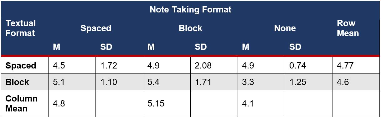
Prior to the in-class examination each participant was asked to sign a consent form in which the ethical considerations were addressed. Individually, the participants were asked to sit in a small study room and were briefed about the
Results
layout of the trial. Then they were handed a passage on a fictional disease, a sheet of instructions for the format of note taking and one ruled A4 paper. They were given 10 minutes to both read the passage and instructions and take notes on the ruled A4 paper. Participants were given the option to move on to the test paper if they wanted to finish the reading section before the 10 minute timer had rung. The two groups with no notes skipped the note taking part and were given the full 10 minutes for reading time. After the reading time, all stimuli and notes were removed and they were handed the test paper that consisted of 9 short answer questions. The participants were given 5 minutes to complete the test paper and were collected at the conclusion of the time limit. The test papers were marked and the results were recorded in a two-way ANOVA for data analysis.
The Journal of Science Extension Research – Vol. 2, 2023 education.nsw.edu.au 128
Table 1 Descriptive statistics of means (M) and standard deviations (SD) for each condition (n=10).
Table 2 Two-way analysis of variance showing the effects of textual format and note taking format on recall. Including sum of squares (SS), degrees of freedom (df), mean square (MS), F-value and p-value.
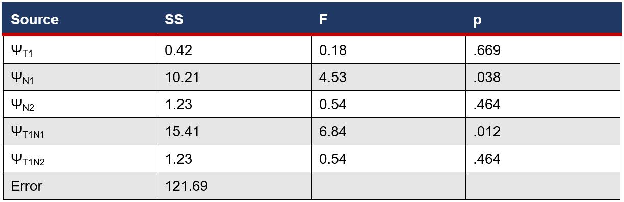
Notes: Subscripts explain main effects of text (T1) and notes (N1, N2), and the interactions between text and notes (T1N1, T1N2).
 Table 3 Sum of squares (SS), observed F-value and p-value results for planned contrasts
The Journal of Science Extension Research – Vol. 2, 2023 education.nsw.edu.au 129
A three level instruction factor was created involving spaced notes, blocked notes and no notes. Table 1 summarises the mean test scores for each formulated condition and their standard deviations. As seen in table 2, it was found that the main effect of paragraph spacing in terms of textual format (F1,54=.18, p=.669).
Table 3 shows that note taking format (F1,54=.54, p=.464) did not yield statistically significant results. There was a significant main effects of notes on test scores, F1, 54=4.53, p=.038. This suggests that an improvement in mean test scores for recalling information resulted by using notes (spaced or block). There were significant interactions between textual format (spaced or block) and notes (notes or no notes), (F1,54= 7.24, p=<.05), this elaborates on the observed significance in interaction seen in Table 2. The mean for blocked text with no notes was 3.3 (SD = 1.25), the mean for blocked text with notes was 5.25 (SD = 1.41), the mean for spaced text with no notes was 4.9 (SD = 0.74), and the mean
for spaced text with notes was 4.7 (SD = 1.87). The interaction effects of textual format and note-taking format were shown to be non-significant, F1,54=.54, p=.464. The mean for blocked text with spaced notes was 5.1 (SD = 1.10), the mean for blocked text with blocked notes was 5.4 (SD = 1.71), the mean for spaced text with spaced notes was 4.5 (SD = 1.72), and the mean for spaced text with blocked notes was 4.9 (SD = 2.08).
Discussion
The results of this study show that in the presence of notes, either block notes or spaced notes, a statistically significant effect was found for recalling information. The improvement in recall was approximately 21% in the notes condition regardless of the type of notes. This holds practical value for the improvement of the study habits of students. It could suggest that the presence of notes in study could improve overall test scores in students, in terms of recalling information. The use of note taking also extends beyond the
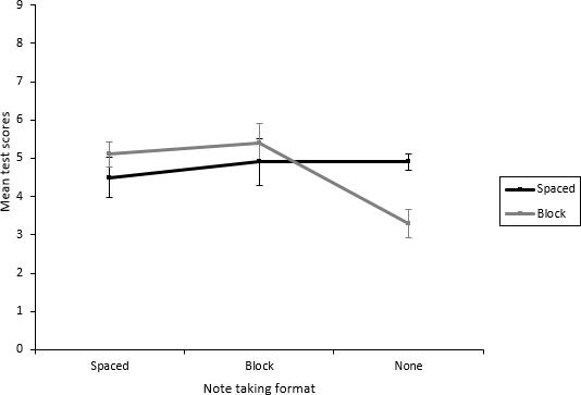 Figure 1. Interaction plot of mean test scores between note taking format and textual format.
The Journal of Science Extension Research – Vol. 2, 2023 education.nsw.edu.au 130
general learning environment and could be used in taking down key information from presentations, speeches and interviews. Recall can drive more informed decision making in workplaces and be applied in any practical situation that involves the application of a set of instructions, such as guidelines for the safe use of equipment in relation to workplace hazards.
Why does the use of notes increase recall? It could be due to the added process of writing and the creation of multimodal stimulation (Udomon et al., 2013), with the pairing of the visual stimulus of the passage. The findings suggest that the absence of the notes creates a setting that yields less cohesion of the given information and translates to lower recall ability of semantic information. As was tested, the results also verify that notetaking is beneficial for the recalling of details of texts (Santa et al., 1979), rather than inferences made from reading between the lines or main points. It could also be suggested that the action of writing notes involves the active organisation of information and requires readers to single out key points, details and filter out unsubstantial details and, thus, contributes to a more efficient retrieval strategy. From this viewpoint, substantiated by the findings, the format of notes (either spaced or blocked) is expendable and can relate to the usefulness of notes overall, regardless of a rigid structure, in the immediate recall of information. However, despite previous findings suggesting the benefit of a rigid note taking structure (Santa et al., 1979), whether the restriction of notes contributes to both cases of textual format is yet to be seen.
The interaction between the presence of notes and textual format suggests that the condition of blocked text with notes yielded the highest recall. An interaction effect was not expected. The single effects of textual format and note-taking format was not significant, however the combined use of textual format in line with the presence of notes was found to have a significant effect on the recall of information. These findings suggest that in the presence of notes, both spaced and blocked text formatting appeared to have no effect on test scores, however blocked text appears to cause a slight increase in test scores. A reason for this could be that blocked text takes up more mental resources to read and interpret as the text is not broken into logical paragraphs and the addition of notes involves rereading the paragraph, and facilitates greater comprehension of the text and reinforces their perception of the text (Millis et al., 1998). In the case of blocked text, note taking facilitates the mental organisation of perceptibly disorganised information, whereas in the case of spaced text with note taking, readers could have used less mental resources in organising the information due to the paragraphing of the passage and could have led to less time spent rereading the text for reinforcement. In turn those with the spaced text might have falsely interpreted their greater grasp of the key details and thus did not engage in the mental task of filtering information, in comparison with those given the blocked text. Thus, the decreased test scores in block text without notes can be explained by the lack of the mentally challenging task of organising the information involved in taking notes. Conversely, the increased test scores in spaced text without notes can be attributed to the perception of
The Journal of Science Extension Research – Vol. 2, 2023 education.nsw.edu.au 131
organised information and perhaps translates to a greater clarity of specific details during the initial reading.
There are points of concern in terms of the methodology of this study. These include the small sample size and the exclusion of the consideration of genders and other ages or literacy levels. The limited range of the participants as a representation of the larger population weighs on the plausibility and the possible generalizability of the results. As such, a conclusive statement cannot be made without considering the possibility of type II errors due to the relatively small number of participants. Despite this, it was observed that there was a small standard deviation across all tested conditions and points to small variability in the study. Also, the lack of access to classrooms, resulted in the use of public areas such as the school library and occupied classrooms persistently throughout the study that could have contributed to the likeliness of systematic errors due to environmental interference. Thus, these methodological limitations open up the consideration for the observed value deviating from the true effects.
There are many other directions to be studied in relation to textual format. The passage used in this study was relatively short, and research can be directed to studying the effect of the length of a piece of information and whether it affects reading comprehension and the retention and ability to recall information immediately. As senior high school students participated in this study, and they were expected to have been more fluent and literate in English, it could be interesting to study the effects of the presence of notes on populations with
lower literacy rates and see if there is a greater effect. The perception of preferred note taking styles could also be explored in concurrence with a similar study to observe whether perceived style correlates with higher rates of recall.
Conclusion
The study focused on the effect of paragraphing and note-taking format on memory recall. The results substantiate the significance of the presence of notes and the significant interaction between the presence of notes and use of paragraphing, in relation to textual format.
Acknowledgement
I would like to acknowledge my mentor, Therese Kanaan, as a major contributor to the development of my project.
References
Gasser, M., Haffeman, J. B. M., & Tan, R. (2005). The Influence of Font Type on Information Recall. North American Journal of Psychology. Retrieved from https://www.researchgate.net/publication/ 237229931_The_Influence_of_Font_Typ e_on_Information_Recall
Larson, K., & Picard, R. (2006). The Aesthetics of Reading. MIT. Retrieved from https://affect.media.mit.edu/pdfs/05.larson -picard.pdf
Ljungdahl, R., & Adler, K. (2018). How Does Text Design Affect Reading
Comprehension Of Learning Materials? Malmo University. Retrieved from https://www.divaportal.org/smash/get/diva2:1534909/FUL LTEXT01.pdf
The Journal of Science Extension Research – Vol. 2, 2023 education.nsw.edu.au 132
Millis, K. K., Simon, S., & TenBroek, N. S. (1998). Resource allocation during the rereading of scientific texts. Memory & Cognition. Retrieved from https://link.springer.com/article/10.3758/B
F03201136
Santa, C., Abrams, L., & Santa, J. (1979). Effects of Notetaking and Studying on the Retention of Prose. Journal of Reading Behavior. Retrieved from https://www.researchgate.net/publication/ 238400613_Effects_of_Notetaking_and_ Studying_on_the_Retention_of_Prose
Udomon, I., Xiong, C., Berns, R., Best, K., & Vike, N. (2013). Visual, Audio, and Kinesthetic Effects on Memory Retention and Recall. (n.p.). Retrieved from https://www.semanticscholar.org/paper/Vi sual-%2C-Audio-%2C-and-KinestheticEffects-on-Memory-UdomonXiong/a188aa5808c6511f71ef81129f7c04
58f8e42e75
The Journal of Science Extension Research – Vol. 2, 2023 education.nsw.edu.au 133
Evolutionary Rate Dynamics of SARS-Cov-2 Variants of Concern Throughout the Covid-19 Pandemic
Owen Yi
James Ruse Agricultural High School
The rapid and widespread transmission of SARS-Cov-2 virus globally has led to substantial molecular evolution in the virus. These mutations have created lineages associated with greater transmissibility among other epidemiological changes and pose a significant global public health threat. In this study, I investigate how the evolutionary rate of SARS-Cov-2 has varied throughout the pandemic. My study included 12 isolates from each of the VOCs to date, 24 non VOC isolates and the Wuhan-Hu-1 reference sequence for a total of 85 sequences. Phylogenetic analysis using a model based on the uncorrelated relaxed clock was performed on these sequences to characterise the evolutionary rate dynamics throughout the pandemic. The results reveal a long but temporary period of rate acceleration around 1.5 times above the mean rate in the Alpha, Gamma and Omicron variants. I suspect that this episodic rate increase is a major factor in the emergence of new VOCs and detail how the “Chronic Infection Hypothesis” could explain the observed rate acceleration. These results reflect the importance of large genomic datasets built upon global genetic surveillance efforts in the understanding of the evolutionary dynamics of SARS-Cov-2 which allow for informed public health decisions.
Literature Review
Severe Acute Respiratory Syndrome
coronavirus 2 (SARS-Cov-2) emerged in late 2019 and is the virus responsible for the coronavirus disease 2019 (Covid-19) pandemic. The Covid-19 pandemic has seen a huge number of SARS-Cov-2 genomes sequenced to understand the virus’s epidemiology. SARS-Cov-2 is an RNA virus with approximately 29000 base pairs. Compared to other RNA viruses, SARS-Cov-2 has a relatively slow mutation rate due to its proof-reading mechanisms e.g. nsp14-ExoN Robson et.al. (2020) which results in a relatively slower substitution rate versus other RNA viruses. Phylogenetic analysis has estimated the pandemic wide substitution rate is between 4.0 × 10⁻⁴ to 1.1 × 10⁻³
Duchene et al. (2020), Ghafari et al. (2022). Despite a relatively slower substitution rate, SARS-Cov-2 has accumulated a large number of mutations throughout the pandemic diverging into multiple different lineages.
Many lineages have developed mutations which affect transmissibility, disease severity, immune escape, diagnostic or therapeutic escape. These lineages which also have established significant transmission are designated as Variants of Interest (VOIs). VOIs that present a significant global health concern are labelled Variants of Concern (VOCs). The only VOCs having existed so far are Alpha, Beta, Gamma, Delta, Omicron. Only Omicron is a currently circulating VOC. New variants are especially a challenge to the global public health
The Journal of Science Extension Research – Vol. 2, 2023 education.nsw.edu.au 134
response and so it is of critical importance to understand the circumstances that give rise to VOCs.
During the pandemic, a huge number of sequenced genomes have been generated as part of a global genomic surveillance effort. These sequences are commonly uploaded to large public databases such as NCBI’s Genbank or GISAID (Global Initiative for Sharing Avian Influenza Data). This genomic data has been leveraged greatly to understand various aspects of SARS-Cov-2 including Covid-19 epidemiology Dellicour et al. (2021), divergence/origin times Pekar et al. (2021), and analyse the impacts of new mutations in the SARS-Cov-2 genome Kraemer et al. (2021) among other phylogenetic analyses. By studying how the evolution of SARS-Cov-2 affects its epidemiology, informed public health decisions can be made in how to respond to the emergence of new variants.
While the large progress has been made in understanding the evolution and epidemiology of SARS-Cov-2, there still remains many open questions. A large gap in our understanding of SARS-Cov-2 is the mechanism by which new variants emerge Tay et. al. (2022). Another relatively underexplored area is the way the evolutionary rate of SARS-Cov-2 has evolved throughout the pandemic. Here, “evolutionary rate” refers to the rate of fixed changes in the virus genome which means I will be measuring the substitution rate (the rate at which mutations become fixed in the genome) rather than purely mutation rate which refers to the frequency that mutations are made during replication. While there are many phylogenetic studies which have yielded estimates for the evolutionary rate of SARS-Cov-2 this only provides a single
rate for the entire pandemic and do not describe in detail the rate variation during the pandemic e.g. if it has accelerated or decelerated. Furthermore, as SARS-Cov2 continues to evolve, new variants have appeared e.g. the Omicron variant and its sub variants Viana et. al. (2022). The Omicron variant is unique in the exceptionally large number of mutations it has compared to the reference sequence even in light of other VOCs. This prompts the question of how the Omicron variant has accumulated so many mutations and so suddenly without detection.
To infer certain parameters describing SARS-Cov-2 e.g. evolutionary rate, divergence times, modern phylogenetic analysis often utilises Bayesian inference. This type of phylogenetic analysis treats parameters in the phylogenetic models as random variables with underlying statistical distributions. These parameters are estimated by sampling using Monte Carlo Markov Chain (MCMC) algorithms to best account for the data e.g. sequences provided. Early phylogenetic analyses assumed a strict molecular clock proposed by Zuckerkandl and Pauling (1962, 1965). These models assumed that the evolutionary rate remained constant across all lineages. This assumption was later shown to be inaccurate in many cases and in the years since, more complex models have been developed to account for rate variation that may be present in a species’ evolution. One such model is the uncorrelated relaxed clock Drummond et.al. (2006). This model gives each branch an independent rate drawn from an underlying distribution e.g. Gamma, Lognormal. Because this model accounts for possible rate variation, it can be used in the phylogenetic analysis to detect rate variation in SARS-Cov-2 throughout the
The Journal of Science Extension Research – Vol. 2, 2023 education.nsw.edu.au 135
pandemic. This allows us to understand how the evolutionary rate has varied in each VOC to better understand the rate dynamics that occur in the emergence of new VOCs.
Scientific Research Question
How has the evolutionary rate of SARSCov-2 varied over the course of the pandemic and what are the possible reasons for the rate variation.
Scientific Research Hypothesis
Due to the quickly changing nature of the SARS-Cov-2 pandemic e.g. accumulation of mutations, changing population dynamics, I hypothesise it is likely that there will be some rate variation in the evolution of SARS-Cov-2.
Methodology
From the NCBI database (https://www.ncbi.nlm.nih.gov/), I looked for all SARS-Cov-2 full genomes that had 0 ambiguous characters throughout the date range of the entire pandemic. From this set, 12 random isolates were sampled for each Variant of Concern (VOC): Alpha, Beta, Gamma, Delta and Omicron. A further 24 isolates which were not of a VOC were randomly sampled. The reference sequence NC_045512 was also included in the dataset. This accounted for 85 genomes sampled for the phylogenetic analysis.
This sampling was preferred over sampling uniformly to ensure sufficient representation of variants less prevalent in the population such as Beta and Gamma. By ensuring there were 12 of each variant in the dataset, the rate characteristics in each variant clade could be explored to a sufficient resolution. The
24 non VOC isolates plus the reference sequence were included to help provide a baseline rate.
The 85 full sequences were aligned using the NCBI multiple alignment tool.
Bayesian phylogenetic inference using Markov Chain Monte Carlo (MCMC) analysis was performed on the 85 sequence dataset using BEAST v.1.10.4. The sequences were divided into taxon sets based on variants. The GTR+Γ4 substitution model was chosen as it leaves all parameters free and accounts for rate heterogeneity. Because the case numbers of Covid-19 fluctuated in waves during the pandemic, the population size model had to be non-parametric and so the GMRF skyride model was chosen. An uncorrelated relaxed clock was used to test for rate variation throughout the evolution of SARS-Cov-2 during the pandemic. MCMC chain length was set to 3 × 10⁷ steps logging every 1 × 10³ steps.
Convergence of all parameters (Effective Sample Size > 200 with burnin of 10%) was verified using Tracer v.1.7.2. A Maximum Clade Credibility Tree was generated using TreeAnnotator v1.10.4 and displayed using FigTree v1.4.4.
To confirm the validity of results and reduce bias, the analysis was rerun using resampled data with the same sampling methodology and BEAST model settings.
Results
According to the results of this phylogenetic analysis, I measured the mean substitution rate for the SARS Cov 2 virus to be 7.64 × 10⁻⁴ substitution per site per year (s/s/y) with a 95% Highest Posterior Density (HPD) interval of (6.77 × 10⁻⁴, 8.52 × 10⁻⁴). The coefficient of
The Journal of Science Extension Research – Vol. 2, 2023 education.nsw.edu.au 136
variation for the substitution rate was 0.35 with a 95% HPD of (0.20, 0.51) revealing moderate rate variation.
Figure 1 shows the Maximum Clade Credibility (MCC) tree. Clades representing Variants of Concern are highlighted. The branches are labelled with the estimated substitution rate for
each branch and are colour coded with red representing a faster rate while blue representing a slower rate. The scale axis represents the time in years since the root of the tree. Table 1 shows the estimated substitution rates for an inferred Most Recent Common Ancestor node
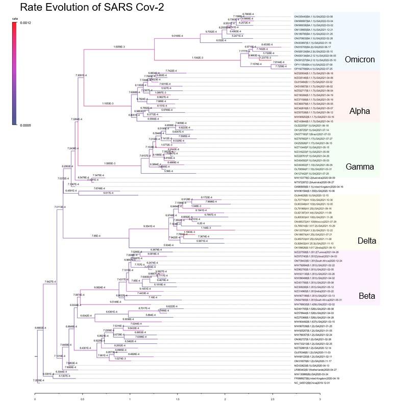
The Journal of Science Extension Research – Vol. 2, 2023 education.nsw.edu.au 137
Figure 1: Maximum Clade CredibilityTree containing 85 isolate genomes. Sequences are labelled by Pango Lineage | Geo location | Collection Date.
Discussion
Evaluation of Phylogenetic Model
Model Strengths
Analysis of the log file in Tracer showed all parameter estimates had reached convergence which helps reduce random error in the MCMC analysis. To test the reliability of this approach, the analysis was rerun with the same phylogenetic model applied to a different dataset of SARS-Cov-2 genomes but resampled using the same sampling procedure for consistency. The parameter estimates were compared with the original model to confirm robustness of the model under similarly sampled but distinct datasets. The parameter estimates had good agreement between the first analysis and rerun analyses indicating robustness of the model and its estimates (Figure 2).
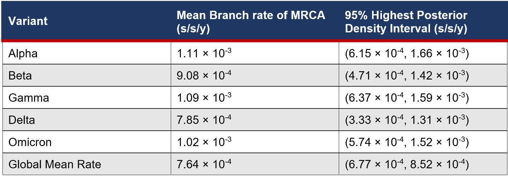
Figure 2: Marginal density plots for the mean rate in both analyses
To confirm the external reliability of these results, I compared the topology of my MCC tree with the NextStrain tree which used the GISAID database. Both trees shared similar topologies for example, the Omicron variant being related to the Alpha variant (being in the same broader clade) but with The Most Recent Common Ancestor (TMRCA) between Alpha and Omicron being very early in the pandemic.
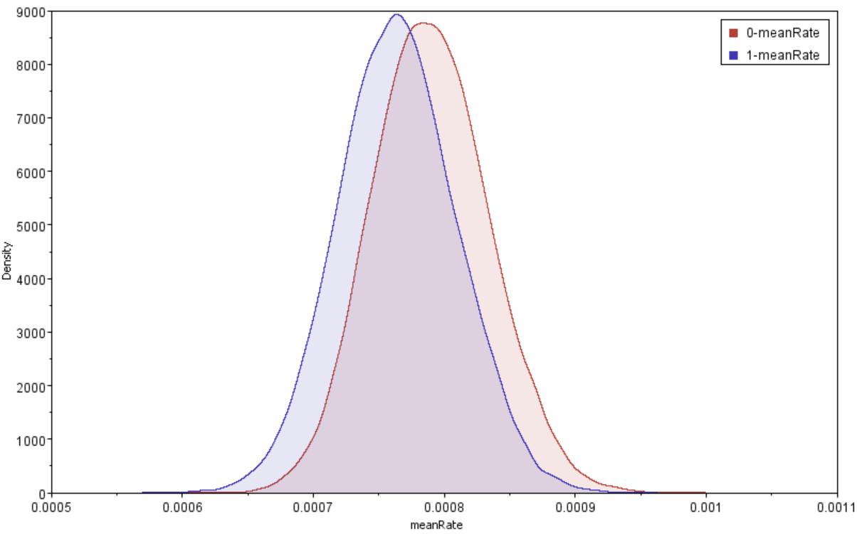 Table 1: Branch substitution rate of the Most Recent Common Ancestor for each variant clade.
The Journal of Science Extension Research – Vol. 2, 2023 education.nsw.edu.au 138
Moreover, the analysis suggests a mean substitution rate of 7.64 × 10⁻⁴ s/s/y (95% HPD: 6.77 × 10⁻⁴, 8.52 × 10⁻⁴. This is consistent with other published results which report rates of 6.7 × 10⁻⁴ to 8.8 × 10⁻⁴ (Duchene et al. 2020) and 4.0 × 10⁻⁴ to 1.1 × 10⁻³. (Ghafari et al. 2022).
Model Limitations
Although the average substitution rate and tree topology agree with external literature, the divergence times are not accurate based on the earliest documented samples for each variant. While the earliest documented sample dates fall within the 95% HPD interval estimates for Alpha, Gamma and Delta, the divergence time estimates for Beta and Omicron are very inaccurate overestimating the divergence time for Beta and underestimating for Omicron.
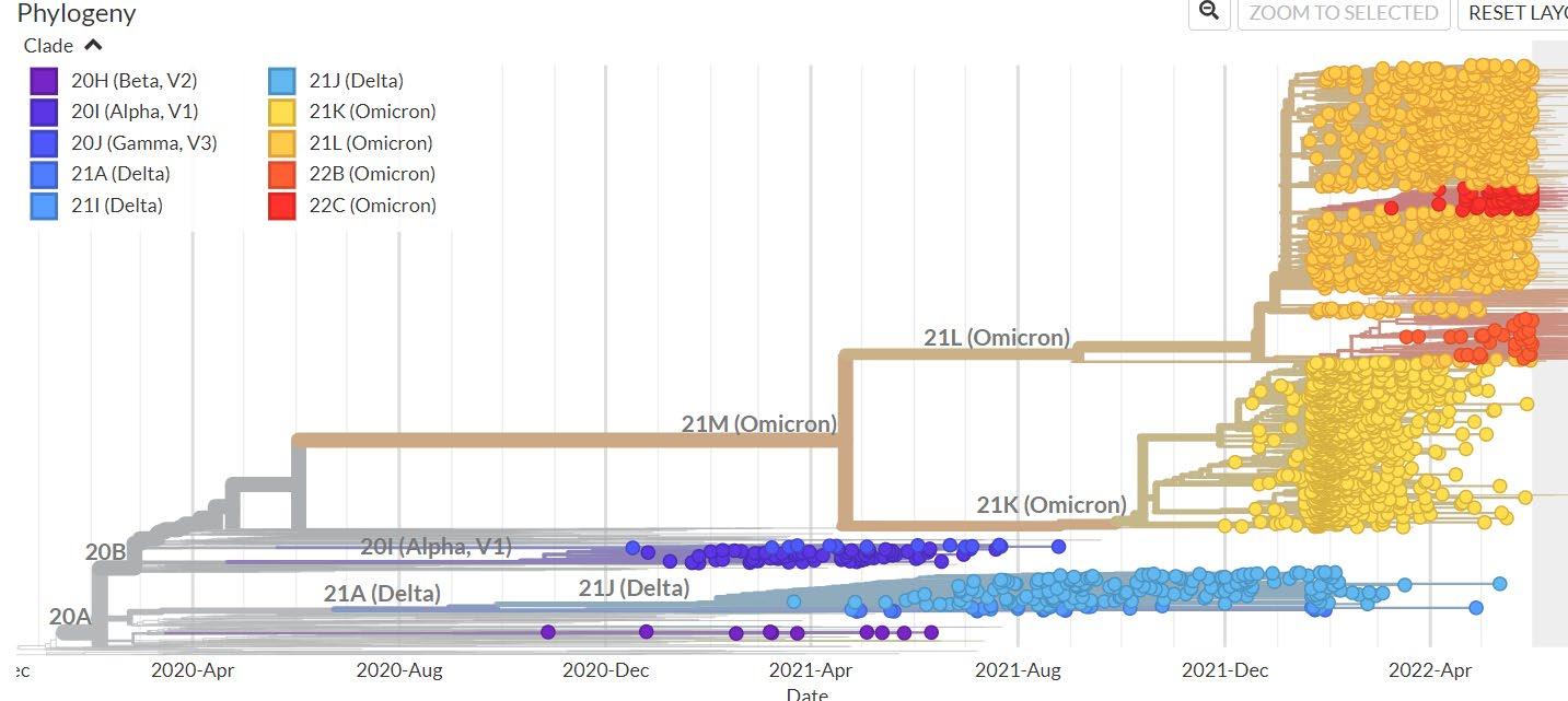
Table 2: Divergence time estimates of variants compared to actual earliest documentation from WHO: https://www.who.int/activities/tracking-SARS-CoV-2-variants
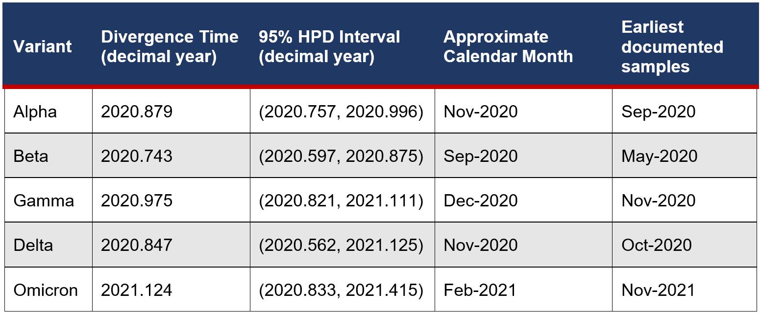 Figure 3: NextStrain SARS-Cov-2 Phylogeny
The Journal of Science Extension Research – Vol. 2, 2023 education.nsw.edu.au 139
The biggest limitation to the results however, is the wide confidence intervals attached to the rate estimates on all the branches. HPD intervals can be narrowed by sampling a larger number of nucleotide sites; however since the analysis used the entire genome length, I am limited by the number of sites on the SARS-Cov-2 genome ~29000 nucleotides. Moreover, the uncorrelated relaxed clock is highly parameter rich which could contribute to more uncertainty in branch rate estimates. Due to the large 95% intervals, there is considerable overlap between the posterior distributions for the branch rates. For most internal branches, the wide uncertainty makes it difficult to determine if the rate variation is noise or if it is reflective of a genuine variation. Thus, my conclusions are based mostly on the clearer extreme cases of rate variation such as the episodic but highly accelerated rates in the TMRCA branches.
Evolutionary Rate Characteristics of SARS-Cov-2
Rate Acceleration in VOCs
From Figure 1, the VOCs Omicron, Alpha and Gamma all appear to have had a long period of faster than normal evolution early on in their respective evolution. The branch rates for the MRCA for each variant is listed in Table 1 revealing that Omicron, Alpha and Gamma, 34%, 45% and 43% increase in substitution rate relative to the global mean rate. Similar to these findings of accelerated rates in VOCs, Rambaut et. al. (2020) found accelerated substitution rate in the Alpha variant. Although the Beta and Delta variants also experienced
a faster substitution rate early on in their evolution, the rate increase is not as extreme compared to the other three VOC. Moreover, the faster mean rate of the Delta MRCA still falls within the 95% HPD of the global mean rate so it is not a substantial increase.
What is also interesting is that these rate increases are episodic and only appear in the internal branches of the variant clades rather than persisting throughout all the tips. This suggests that the increases in the substitution rate are due to temporary environmental factors rather than fixed genetic changes e.g. mutations to the replication or proof-reading machinery. This result is in agreement with Tay et. al. (2022) concluding that “episodic, instead of long term, increases in the substitution rate underpin the emergence of VOCs”. However, unlike the several fold faster rates in VOC compared to the background rate found by Tay et. al. our analysis shows much smaller rate increases (see Table 1). This discrepancy could be explained by purifying selection where there is a time lag for natural selection to remove deleterious mutations Ghafari et al. (2022) and so later analyses may find slower substitution rates.
These episodic accelerated substitution rates help explain how some of these variants for example the Omicron variant (which has accumulated 50 mutations Martin et. al. (2021) before being first identified) could have mutated so much without being detected.
Chronic Infection Hypothesis” Provides a Possible Account for Rate Acceleration in VOCs.
The Journal of Science Extension Research – Vol. 2, 2023 education.nsw.edu.au 140
A plausible theory which accounts for these episodic rate increases explains that “co-infection and subsequent genome recombination” Ou et. al. (2022) is driving the accelerated evolution of Covid-19 variants. Recombination occurs when two different strains co-infect a cell and as a result, genetic material is shuffled around in the virus progeny. Yi et. al. (2020) has indicated that SARSCov-2 has also evolved through recombination as well as simple mutation, proving that recombinant genomes were present in the Covid-19 population.
Together this evidence supports the “chronic infection hypothesis” Chaguza et. al. (2022). The “chronic infection hypothesis” explains the long fast branches in Figure 1. Chronic infection in immunocompromised individuals provides the right environmental conditions for accelerated evolution. This is because lengthy chronic infections provide the virus both more time and a weaker immune system which “may allow an exploration of the SARS-CoV-2 fitness landscape” Harari et. al. (2022) producing the right selective pressures to mutate more. Moreover, patients with chronic infection are also more likely to develop co-infections with multiple Covid-19 strains increasing the likelihood of recombination. This also accounts for how these mutations could remain undetected because genetic sequencing along the transmission chains of acutely infected individuals would fail to detect intrahost evolution.
However, this hypothesis alone is insufficient to explain all the rate variation in the phylogenetic tree. For example, the Delta and Beta variants did not experience substantial rate acceleration and so may have evolved through simple
mutations. Some tip branches scattered across all variant clades also appear to have an accelerated rate although it is unclear if it is genuine rate variation or due to the stochasticity of the MCMC estimation.
Improvements and Further Inquiry Improvements
More non-phylogenetic data could be incorporated into the model to improve the accuracy of rate estimates. For example, the age of the different variants based on the first identified samples could be specified in the model to fix divergence times for different variant clades. Since genetic distance is the product of substitution rate and divergence time, specifying accurate divergence times could lead to more accurate rate estimations.
Additionally, different tree priors e.g. Bayesian skyline, Yule process speciation could be tested to analyse if these results still hold under different models Möller et. al. (2018). The tree prior model with the highest statistical fit could be compared using a Log Bayes Factor to inform which tree prior best represents the evolutionary process of SARS-Cov-2.
Further Inquiry
To better test the “Chronic Infection Hypothesis”, genome sequences stratified by whether or not the infection was chronic. The same evolutionary rate analysis could be used on both data sets and compared to see if there is any difference in rate dynamics from SARSCov-2 in chronically ill patients. This data may be harder to find as infection period may not be labelled to sequences for genome databases.
The Journal of Science Extension Research – Vol. 2, 2023 education.nsw.edu.au 141
Genomic surveillance could be extended to serially sample Covid-19 sequences from chronically infected patients to analyse in real time the evolution of Covid-19. Phylogenetic analysis could be used to explore the specific intrahost evolution of Covid-19.
Specific mutations could be analysed in different isolates to explore if changes in the underlying mutation rate due to genetic factors e.g. replication/proofreading mechanisms is contributing to the observed rate variation. Coronaviruses are able to “proof-read and remove mismatched nucleotides during replication and transcription” Robson et.al. (2020). While most mutation analysis is focused on the spike proteins as these can affect transmissibility and vaccine efficacy, mutations on the SARSCov-2 proof-reading complex could be analysed in tandem with phylogenetic analysis to understand the genetic factors that can lead to rate variation.
Conclusion
In this paper, I found that in the evolution of certain Variants of Concern of the SARS-Cov-2 virus namely the Alpha, Gamma and Omicron variants displayed a noticeable and long period of accelerated substitution rates early on in their emergence before the substitution rate slowed back down towards the mean level upon establishing in the population. The other VOCs Beta and Delta also displayed some rate acceleration early in their evolution however to a much lesser extent. I note that the analysis is limited by the wide HPD intervals attached to the branch rate estimates which makes it harder to discern between genuine rate variation and noise for most internal branches. I point to the “Chronic Infection
Hypothesis” as a possible explanation for the observed rate variation. Under this hypothesis, prolonged infection in immunocompromised patients allows the virus to accumulate mutations faster leading to the emergence of new variants. This model provides a good explanation for the long periods of rate acceleration which occur immediately before the emergence of the Alpha, Gamma and Omicron variants.
More genomic surveillance especially to more densely sample SARS-Cov-2 sequences during prolonged infection is required to further investigate intrahost evolution to test the “Chronic Infection Hypothesis”. To investigate other possible causes of the observed rate evolution, mutational analysis of genes in the SARS-Cov-2 genome associated with viral replication such as proof-reading could be corroborated against changes in substitution rate to test if genetic factors are contributing to the rate variation.
These results reflect the importance of large public genomic datasets built upon global genetic surveillance efforts in the understanding of the evolutionary dynamics of SARS-Cov-2. Further analysis on the exact circumstances under which new Variants of Concern arise will be crucial to the global health response to the Covid-19 pandemic to prepare for the emergence of new variants of epidemiological significance.
Acknowledgements
I thank my research mentors Dr. Carina Dennis, Dr. Jiaojiao Li and Dr. Mathieu Fourment for their invaluable advice during discussions to answer technical questions and provide useful suggestions.
The Journal of Science Extension Research – Vol. 2, 2023 education.nsw.edu.au 142
References
Chaguza, C et. al. 2022. “Accelerated SARS-CoV-2 intrahost evolution leading to distinct genotypes during chronic infection”. MedRxiv, 2022.06.29.22276868; doi: 10.1101/2022.06.29.22276868
Drummond, Alexei J et al. 2002. “Estimating mutation parameters, population history and genealogy simultaneously from temporally spaced sequence data.” Genetics, vol. 161, no. 3. pp, 1307-20.
doi:10.1093/genetics/161.3.1307
Drummond, Alexei J et. al. 2006. “Relaxed phylogenetics and dating with confidence.” The Public Library of Science Biology, vol. 4, no. 5. e88. doi:10.1371/journal.pbio.0040088
Duchene, S. et.al. 2020. “Temporal signal and the phylodynamic threshold of SARSCoV-2”, Virus Evolution, vol. 6, no. 2.
https://doi.org/10.1093/ve/veaa061
Fourment, M. Darling, A.E. (2018). “Local and relaxed clocks: the best of both worlds”. PeerJ, 6:e5140
https://doi.org/10.7717/peerj.5140
Ghafari, M. et. al. 2022. “Purifying Selection Determines the Short-Term Time Dependency of Evolutionary Rates in SARS-CoV-2 and pH1N1 Influenza”, Molecular Biology and Evolution, vol. 39, no. 2. msac009.
https://doi.org/10.1093/molbev/msac009
Harari, S. Tahor, M. Rutsinsky, N. et al. 2022. “Drivers of adaptive evolution during chronic SARS-CoV-2 infections”. Nature Medicine, vol. 28, pp. 1501–1508. https://doi.org/10.1038/s41591-02201882-4
Hu, B et. al. 2021. “Characteristics of SARS-CoV-2 and COVID-19.” Nature Reviews. Microbiology, vol. 19, no. 3, pp. 141-154. doi:10.1038/s41579-020-004597
Kayla, M.P. Lauring, A.S. 2018. “Complexities of Viral Mutation Rates”. Journal of Virology, vol. 29, no. 14, pp. DOI: https://doi.org/10.1128/JVI.01031-17
Lynch, M. 2010. “Evolution of the mutation rate.” Trends in genetics, vol. 26, no. 8, pp. 345-52. doi:10.1016/j.tig.2010.05.003
Martin, D et. al. 2022. “Selection analysis identifies unusual clustered mutational changes in Omicron lineage BA.1 that likely impact Spike function”, BioRxiv.
https://doi.org/10.1101/2022.01.14.47638 2
Minin, V. N. et.al. 2008. “Smooth Skyride through a rough Skyline: Bayesian coalescent-based inference of population dynamics.” Molecular Biology and Evolution, vol. 25, no. 7, pp. 1459-1471. doi:10.1093/molbev/msn090
Möller, S et al. 2018. “Impact of the tree prior on estimating clock rates during epidemic outbreaks” Proceedings of the National Academy of Sciences, vol. 115, no. 16, pp. 4200-4205. doi.org/10.1073/pnas.1713314115
NCBI. 2022. “NCBI Virus”, https://www.ncbi.nlm.nih.gov/labs/virus/vs si/#/virus?SeqType_s=Nucleotide
Nextstrain. 2022. “Genomic epidemiology of SARS-CoV-2 with subsampling focused globally over the past 6 months”, https://nextstrain.org/ncov/gisaid/global/6 m
The Journal of Science Extension Research – Vol. 2, 2023 education.nsw.edu.au 143
Ou, J. Lan, W. Wu, X. et. al. 2020. “Tracking SARS-CoV-2 Omicron diverse spike gene mutations identifies multiple inter-variant recombination events”. Signal Transduction and Targeted Therapy, vol. 7, no. 138.
https://doi.org/10.1038/s41392-02200992-2
Rambaut, A. Loman, N. Pybus, O et. al. 2020 (CoG-UK). “Preliminary genomic characterisation of an emergent SARSCoV-2 lineage in the UK defined by a novel set of spike mutations.”
https://virological.org/t/preliminarygenomic-characterisation-of-anemergent-sars-cov-2-lineage-in-the-ukdefined-by-a-novel-set-of-spikemutations/563
Robson, F et al. 2020. “Coronavirus RNA Proofreading: Molecular Basis and Therapeutic Targeting.” Molecular cell, vol. 79, no. 5, pp. 710-727.
doi:10.1016/j.molcel.2020.07.027
Tavaré, S. 1986. “Some probabilistic and statistical problems in the analysis of DNA sequences.”
Tay, J H et al. 2022. “The Emergence of SARS-CoV-2 Variants of Concern Is Driven by Acceleration of the Substitution Rate.” Molecular biology and evolution vol. 39, no. 2: msac013. doi:10.1093/molbev/msac013
Viana, R., Moyo, S., Amoako, D.G. et al. 2022 “Rapid epidemic expansion of the SARS-CoV-2 Omicron variant in southern Africa”. Nature, vol. 603, pp. 679–686 (2022). https://doi.org/10.1038/s41586022-04411-y
WHO. 2022. “Tracking SARS-Cov-2 variants”
https://www.who.int/activities/trackingSARS-CoV-2-variants
Yang, Z, Rannala, B. 2012 “Molecular phylogenetics: principles and practice” Nature Reviews Genetics, vol. 13, pp. 303–314. https://doi.org/10.1038/nrg3186
Yi, H. 2020. 2020. “2019 Novel Coronavirus Is Undergoing Active Recombination”. Clinical Infectious Diseases, vol. 71, no. 15, pp. 884–887, https://doi.org/10.1093/cid/ciaa219
Yi, K., Kim, S.Y., Bleazard, T. et al. 2021. “Mutational spectrum of SARS-CoV-2 during the global pandemic”. Experimental and Molecular Medicine, vol. 53, pp. 1229–1237.
https://doi.org/10.1038/s12276-02100658-z
Zuckerkandl E, Pauling L. 1962. “Molecular disease, evolution and genetic heterogeneity”. Horizons in biochemistry, pp. 189–225.
Zuckerkandl E, Pauling L. 1965. “Evolutionary divergence and convergence in proteins.” Evolving genes and proteins. New York: Academic Press. p. 97–166.
Appendix
Google Drive Link to Supplementary Data
The Journal of Science Extension Research – Vol. 2, 2023 education.nsw.edu.au 144
A Comparison of the Concentration of Lycopene in Australian
and Italian Canned Tomatoes
Jacob Hill St Ives High School
Lycopene, a carotenoid commonly found in tomatoes and other red fruits has powerful antioxidant properties that combat free radicals in the body. This study aimed to determine if there is a difference in the concentration of lycopene in tinned tomatoes from different regions, namely, Australia and Italy. Lycopene concentration can be measured using colourimetry after it has been dissolved into a solution of hexane:BHT:acetone. This study revealed that the lycopene concentration of canned tomatoes from Italy and Australia was not significantly different with a P value of 0.768. Consuming foods and meals made with tomatoes sourced locally or from Italy will provide the same amount of lycopene and thus the same antioxidant properties and health benefits.
LITERATURE REVIEW
Antioxidants are a group of organic compounds that promote health in the human body by counteracting free radicals. Free radicals are compounds with unpaired valence electrons. Their unpaired valence electrons, give them the ability to either donate or accept a proton making them highly reactive (Martemucci, et al., 2022).
Free Radicals are created in the body from metabolic processes, usually they are beneficial, helping with the destruction of pathogens. However, free radicals also enter the body from external sources such as, smoking, x-rays, air pollutants and ozone. This can cause an excess of free radicals and this imbalance causes oxidative stress resulting in damage to the membranes and contents of cells. The action of free radicals has been linked to heart disease, increased risk of stroke, diabetes, cancer, macular degeneration and general acceleration of
ageing (Lerner & Lerner, 2014 and Ashok, 1999).
Lycopene (C40H56) (Figure 1) is a long chain hydrocarbon molecule classified as a carotenoid. Carotenoids are a class of red pigments with antioxidant properties that are found in many fruits and vegetables. Lycopene has the greatest antioxidant ability of the carotenoids and is one of the major carotenoids found in foods (Zhou, et al., 2016). Consuming lycopene has been linked to reduced risk of cancers, particularly prostate cancer and decreased oxidisation of cholesterol (Górecka, et al., 2020 and NHMRC 2017).
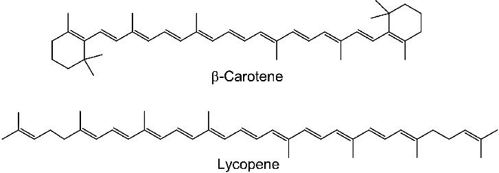
The Journal of Science Extension Research – Vol. 2, 2023 education.nsw.edu.au 145
Figure 1; Chemical structures of Lycopene and β-carotene (Gumus & Turker, 2014)
The National Health and Medical Research Council, (NHMRC, 2017) recognises the antioxidant benefits of lycopene, however, they do not give a level of recommended intake. Other studies suggest that intakes between 8–21mg per day appear to be most beneficial (Petre, 2018). The greatest dietary sources of lycopene include red fruits and vegetables such as tomatoes, watermelon, carrots, pink guava, papaya and dried apricots. Unfortunately, Australian studies reveal that only 3.7% of children from the ages of 14-18 met their dietary requirements for vegetables in 2015 (AIHW, 2022). There is evidence that up to 80% of dietary lycopene comes not from fresh fruit and vegetables but from processed tomato products used in foods such as pizza and pasta (Zhou, et al., 2016 and Górecka, et al., 2020).
With the majority of dietary lycopene coming from processed tomato products it raises questions regarding the lycopene content in processed tomatoes. This study will investigate the difference in concentration of lycopene levels in processed tomato products originating from different areas. Góreka, et al. (2020) states that the concentration of lycopene in tomatoes correlates to the time that the tomatoes spend in the sun. Australian consumers can generally access both Australian and Italian tomatoes which are readily available in Australian supermarkets. Tomatoes are a summer crop, since Italy has comparatively longer days in summer than Australia, this could signify a greater lycopene concentration in Italian tomatoes over Australian. There are many other factors that could affect the lycopene content in addition to sunlight such as the manufacturing processes and time taken to transport to the supermarkets. It is not known if this
creates a significant difference between the lycopene content of these products (Górecka, et al., 2020).
A review of the literature revealed multiple studies with methods for extracting and measuring lycopene from tomato products using colourimetry. Colourimetry studies were very similar across all studies with minor differences regarding mass of product tested, volumes of solution used, and time taken to stir the solution.
A 2:1:1 Hexane:Ethanol:Acetone (solvent solution) mixture is needed to dissolve the lycopene and separate it from the tomato. After stirring, adding water causes the solution to separate into polar and non-polar layers. The top, coloured, layer containing non-polar molecules dissolved in hexane is then analysed using colourimetry at 503nm (Alda, et al., 2009; Adejo, et al., 2015; Fish, 2002; Fish, et al., 2003; Suwanaruang, 2016; Anthon & Barret, 2007; de Montemas, 2020).
To prevent the oxidation of lycopene, some studies dissolved butylated hydroxytoluene (BHT) in ethanol prior to its addition into the solvent solution. BHT is a synthetic antioxidant commonly used as a preservative because it oxidises preferentially to other compounds. This prevents the lycopene in solution from being oxidised (Anthon & Barret, 2007).
Lycopene will oxidise by photo-oxidation in the presence of light (MartínezHernández, et al., 2016). In food products, oxidation of lycopene is undesirable as it reduces the oxidative ability of the food and results in loss of beneficial antioxidant properties. Fish, (2002) states that the absorbance of lycopene in solution decreases at 1% per
The Journal of Science Extension Research – Vol. 2, 2023 education.nsw.edu.au 146
hour when stored in amber vials under fluorescent lighting. This provides evidence of the constant degradation of lycopene in light and provides incentive to use of BHT as a preservative.
Lycopene is not the only red pigmented carotenoid present in tomatoes. βcarotene is a prevalent antioxidant having the same chemical formula of C40H56 and a similar absorbance spectra to lycopene. β-carotene is the second most prevalent carotenoid in fresh tomatoes having a concentration of 15% relative to lycopene (Anthon & Barret, 2007).
Lycopene and β-carotene have slightly differing absorbance spectra. Testing the absorbance at 503nm and then again at 444nm enables the concentration of Lycopene and β-carotene to be calculated using the Beer-Lamberts law. This equation states there is a linear relationship between the concentration and the absorbance of the solution. To calculate absorbance, the extinction coefficient is needed. This is the amount of light absorbed by a compound at a specific wavelength per concentration (MolL-1) per optical path length (cm) (Anthon & Barret, 2007).
When considering both the absorbance of lycopene and β-carotene, the following equations are needed.
wavelengths of light the values correspond to.
These equations are rearranged into equation 2 which will be used to calculate concentration from the absorbance values gathered.
Equation 2. Relating the absorbance values and extinction coefficients to find concentration of lycopene
SCIENTIFIC RESEARCH QUESTION
Do cans of tomatoes from different regions contain similar concentrations of lycopene.
SCIENTIFIC HYPOTHESIS
There is negligible difference in the concentration of lycopene in Italian and Australian canned tomatoes available to Australian consumers.
METHODOLOGY
Preparation of solvent
A solution of 2:1:1 Hexane:BHT:Acetone (solvent solution), was used in the extraction of lycopene. The BHT solution was created as a 0.5%(w/v) BHT in ethanol solution. 20 ml of freshly made solvent solution was added to three 25ml conical flasks.
Preparation of Tomatoes
Equation 1. Where ε is the extinction coefficient, A is the absorbance, C is the concentration and optical path length is omitted because in a colourimeter this is 1. Subscript L is used to signify the concentration and extinction coefficients of lycopene and β for β-carotene. Subscript 444 and 503 to signify the
A tin of pre-chilled diced tomato was opened and half was placed into a beaker and blended using a handheld blender. Approximately one gram of tomato was weighed and placed into each conical flask.
The Journal of Science Extension Research – Vol. 2, 2023 education.nsw.edu.au 147
Extraction of lycopene
Conical flasks were covered with plastic wrap to decrease loss of solvent by evaporation. Each sample was stirred for 15 minutes using magnetic stir bars. carotenoids were dissolved into the solvent solution. 10 mL of water was then added into the solution where two distinct layers formed.
Colourimetry
Colourimetry was conducted using PASCO PS-2600 spectrometer and standardised quartz cuvettes. The colourimeter was calibrated using hexane. The top layer of each solution was tested for absorbance at 444 and 503nm and was tested twice at each wavelength. The concentration of lycopene was calculated using Equation 2.
RESULTS
Ten tins of tomatoes were tested, with three samples were taken from each tin. Each sample was then run through the colorimeter twice to reduce the impact of random error in the data. For each test the concentration of lycopene was
calculated. Outliers were considered as any values 2 standard deviations away from the mean and were removed. Results from each tin were then averaged for statistical testing Table 1.
t-Test: Two-Sample Assuming Equal Variances
t
An f test was performed with α value of 0.05 that gave a p value of 0.1218425 (shown in appendix) showing an insignificant difference in the variance of data sets. Two tailed t-test was preformed to investigate a difference in means of the two data sets. As shown in Table 1 it produced a P value of 0.768 which is an insignificant difference between results
Australian Italian Mean 21.6326138 21.4472161 Variance 2.66230031 1.185041446 Observations 10 10 Pooled Variance 1.92367088 Hypothesized Mean Difference 0 df 18 t Stat 0.29889862 P(T<=t) one-tail 0.38422041
Critical one-tail 1.73406361
two-tail 0.76844082
t
P(T<=t)
Critical two-tail 2.10092204
Table 1. t-test results
The Journal of Science Extension Research – Vol. 2, 2023 education.nsw.edu.au 148
There was an inverse relationship between the calculated concentration of lycopene and the mass of tomato used in testing (Figure 3).
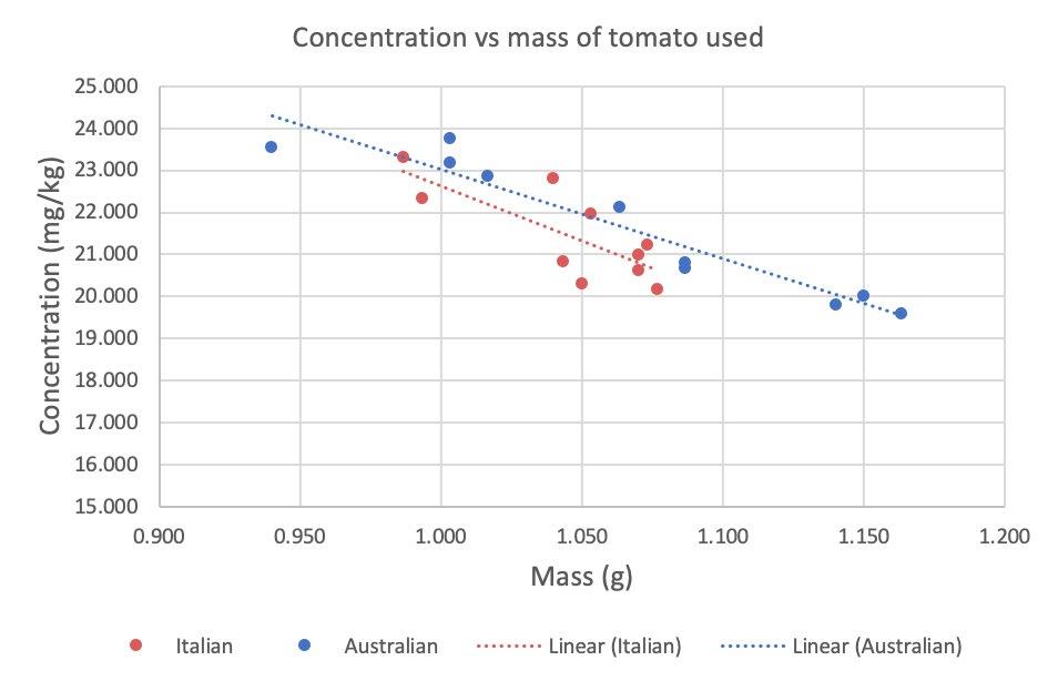
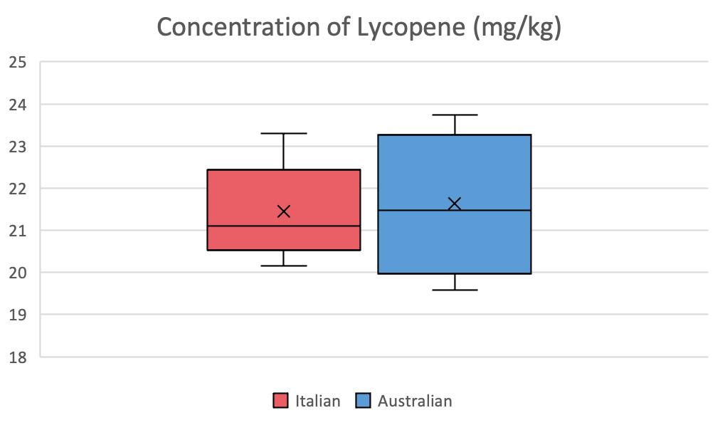 Figure 2. Graphical representation of the five-number summary of concentration of Lycopene in Australian and Italian tins of diced tomatoes. The Average concentration of lycopene in milligrams of lycopene per kilogram of tomato for Australian tomatoes was 21.633 and 21.447 for Italian.
Figure 3. Concentration of lycopene vs mass of tomato mass
Figure 2. Graphical representation of the five-number summary of concentration of Lycopene in Australian and Italian tins of diced tomatoes. The Average concentration of lycopene in milligrams of lycopene per kilogram of tomato for Australian tomatoes was 21.633 and 21.447 for Italian.
Figure 3. Concentration of lycopene vs mass of tomato mass
The Journal of Science Extension Research – Vol. 2, 2023 education.nsw.edu.au 149
DISCUSSION
This report aimed to determine if there is a significant difference in the concentration of lycopene in canned tomatoes from Australia and Italy. This investigation provides insight into the differences, or lack thereof between concentrations of lycopene in Australian and Italian canned tomatoes. Due to its antioxidant abilities, lycopene is an important molecule and diced tomatoes with higher concentration of lycopene are more desirable.
The results revealed that to a confidence interval of 95%, the calculated P value of 0.768 was much greater that the 0.05 needed to indicate a significant difference. This supports the hypothesis that there was no significant difference in the concentration of lycopene in Australian and Italian canned tomatoes.
The results also revealed an inverse relationship between concentration of lycopene and mass of tomato (Figure 3) which was an unexpected trend. Since the mass of the tomato is considered when calculating the concentration of lycopene per kg of tomato, it was anticipated that this gradient would trend near zero. This trend may be a result of time stirring solution, which was kept consistent at 15 minutes or until colouration of tomato was lost. Lycopene from samples of tomato with a higher mass may not have been fully dissolved into solution when stirring was completed.
A number of processes were employed to ensure data validity. Due to the volatility, fresh solvent was used regularly through the experiment to ensure that components were in their required concentrations.
Repetitive testing of the same cans of tomato and averaging of data collected served to remove the impact of random error on the experiment and increase its reliability.
All equipment used in this study was rinsed three times in a dishwasher without the use of detergent which would act as an emulsifying agent, preventing the separation of the solution into layers as is required in the method.
Multiple studies have been conducted on lycopene levels in fresh tomatoes and there is a wide variation in results are as follows; 6.6 – 490 mg/kg (Fish, et al., 2003); 120mg/kg (Alda, et al., 2009); 29.4mg/kg (Górecka, et al., 2020); 104.699mg/kg (Suwanaruang, 2016); 25 – 6700 mg/kg (Martínez-Hernández, et al., 2016). The results that have been collected in this experiment at 21.632 and 21.447 mg/kg are consistently lower than a number of the studies described in literature. This may be worth investigating, to determine if tinned tomatoes have a lower concentration of lycopene than fresh tomatoes. This difference could also be indicative of systematic error present in the method. However, systematic error that may have occurred in the experiment has little bearing on the conclusion as the hypothesis of the experiment was to investigate a difference and as long as random error was removed from the method, then conclusions drawn from the experiment are valid.
Drawbacks were encountered with the software that was used because of its inability to select specific wavelengths. However, this did not impact the overall results of the study and only resulted in
The Journal of Science Extension Research – Vol. 2, 2023 education.nsw.edu.au 150
increasing the time taken for the absorbance to be measured.
An extension of this study could further investigate the trend that arose in the concentration of lycopene and the mass of tomato tested. This would involve testing smaller and larger masses of tomato to investigate if the trend continued. Suwanaruang, (2016) used 0.001g of tomato and 8 mL of solvent solution which is 0.000125 g of tomato per mL of solvent compared to the 0.05g/ml used in this study. Testing with ratios such as this may yield a more consistent result for the concentration of lycopene. However, due to limitations in the accuracy of scales available, a mass of 1g was chosen as to increase the number of significant figures. As lycopene is soluble in hexane to 1g/L (PubChem, 2022), and initial testing with 1g of tomato showed a mass of dissolved lycopene in 20mL of hexane to be 2.187 x10^-5g. or 0.0010935 g/L solubility wasn’t perceived as an issue.
Variations on this study could investigate the concentration of lycopene in different tomato products that are commonly found in a western diet and compare them to the concentration of a fresh tomato. The results of an investigation of this idea would depend of the amount of processing that was done, largely the removal of water which makes up a majority of a tomatoes mass. This would be a further extension of this study and an opportunity to not only study one ingredient but to study whole foods and extrapolate to average quantities consumed by teenagers, and consider which meals would give greater lycopene content and thus greater antioxidant benefits.
CONCLUSION
This report investigated whether there was a difference in lycopene concentration between Australian and Italian diced canned tomatoes. The results of this experiment support the hypothesis stating that there is an insignificant difference in lycopene concentration. There was a low random error in the experiment allowing for the above conclusion to be drawn irrespective of the presence of systematic error because of its equal affect to both Australian and Italian tomato tests.
Irrespective of any systematic error that was present reducing the accuracy, effecting the concentration of lycopene in both the Australiana and Italian tomatoes. the conclusion that has been drawn from the experiment is valid because of the removal of random error from the experimental method. For the average Australian consumer, purchasing either locally grown or Italian tomatoes will provide the same lycopene intake and associated health benefits of reduction in risk of cancer, stroke and diabetes. There may be other factors that influence consumers’ product choice such as supporting locally grown produce, farmers and industry and reducing the environmental impact of transport of tomatoes grown overseas. However, Australian consumers can be reassured that both the Australian and Italian tomatoes on their local supermarket shelves are equal in their lycopene concentrations and thus health benefits.
The Journal of Science Extension Research – Vol. 2, 2023 education.nsw.edu.au 151
REFERENCES
Adejo, G., Agbali, F. & Otokpa, O., 2015. Antioxidant, Total Lycopene, Ascorbic Acid and Microbial Load Estimation in Powdered Tomato Varie. OALib, 02(08), pp. 1-7.
AIHW, 2022. Australia's health 2018, Fruit and vegetable intake - Australian Institute of Health and Welfare. [Online] Available at:
https://www.aihw.gov.au/reports/australia s-health/australias-health2018/contents/indicators-of-australiashealth/fruit-and-vegetable-intake
[Accessed January 2022].
Alda, L. et al., 2009. Lycopene content of tomatoes and tomato products. Journal of Agroalimentary Processes and Technologies, 15(4), pp. 540-542.
Anthon, G. & Barret, D., 2007. Standardization of a Rapid Spectrophotometric Method for Lycopene Analysis. Acta Horticulturae, pp. 111-128.
de Montemas, A., 2020. Storage temperature and its effect on the concentration of Lycopene extracted from tomatoes. Scientific Research in School, 2(1), pp. 61-66.
Fish, W., 2002. A Quantitative Assay for Lycopene That Utilizes Reduced Volumes of Organic Solvents. Journal of Food Composition and Analysis, 3(15), pp. 309-317.
Fish, W., Davis, A. & Perkins-Veazie, P., 2003. A rapid spectrophotometric method for analyzing lycopene content in tomato and tomato products. Postharvest Biology and Technology, 28(3), pp. 425-430.
Gumus, S. & Turker, L., 2014. TG Index, its Graphical Matrix Representation and Application on Polyenes. Bulletin of the Korean Chemical Society, May, 35(5), pp. 1413-1416.
Górecka, D. et al., 2020. Lycopene in tomatoes and tomato products. Open Chemistry, 18(1), pp. 752-756.
Lerner, K. & Lerner, B., 2014. Antioxidants. World of Sports Science.
Martemucci, G. et al., 2022. Free Radical Properties, Source and Targets, Antioxidant Consumption and Health. Oxygen, 12 April, 2(2), pp. 48-78.
Martínez-Hernández, G. B. et al., 2016. Processing, Packaging, and Storage of Tomato Products: Influence on the Lycopene Content. Food Engineering Reviews, 8(1), pp. 52-75.
National Health and Medical Research Council, 2017. Nutrient Reference Values for Australia and New Zealand. [Online]
Available at:
https://www.nhmrc.gov.au/sites/default/fil es/images/nutrient-refererence-dietaryintakes.pdf [Accessed 26 Feb 2022].
Petre, A., 2018. healthline. [Online]
Available at:
https://www.healthline.com/nutrition/lycop ene#:~:text=There%20is%20currently%2 0no%20recommended,appear%20to%20 be%20most%20beneficial.&text=Most%2 0red%20and%20pink%20foods,richest% 20sources%20of%20this%20nutrient [Accessed 26 2 2022].
Porrini, M. & Riso, P., 2005. What Are Typical Lycopene Intakes. The Journal Of Nutrition.
The Journal of Science Extension Research – Vol. 2, 2023 education.nsw.edu.au 152
PubChem, 2022. PubChem. [Online]
Available at:
https://pubchem.ncbi.nlm.nih.gov/compou nd/Lycopene [Accessed 24 August 2022].
Suwanaruang, T., 2016. Analyzing Lycopene Content in Fruits. Agriculture and Agricultural Science Procedia, Volume 11, pp. 46-48.
Zhou, Y. et al., 2016. Plasma Lycopene Is Associated with Pizza and Pasta Consumption in Middle-Aged and Older African American and White Adults in the Southeastern USA in a Cross-Sectional Study. PLOS ONE, 11(9), p. N.A..
APPENDIX
F-Test Two-Sample for Variances
Statistical analysis of variance using an f test
Collection of data collected from each can of tomatoes after averaging of raw data
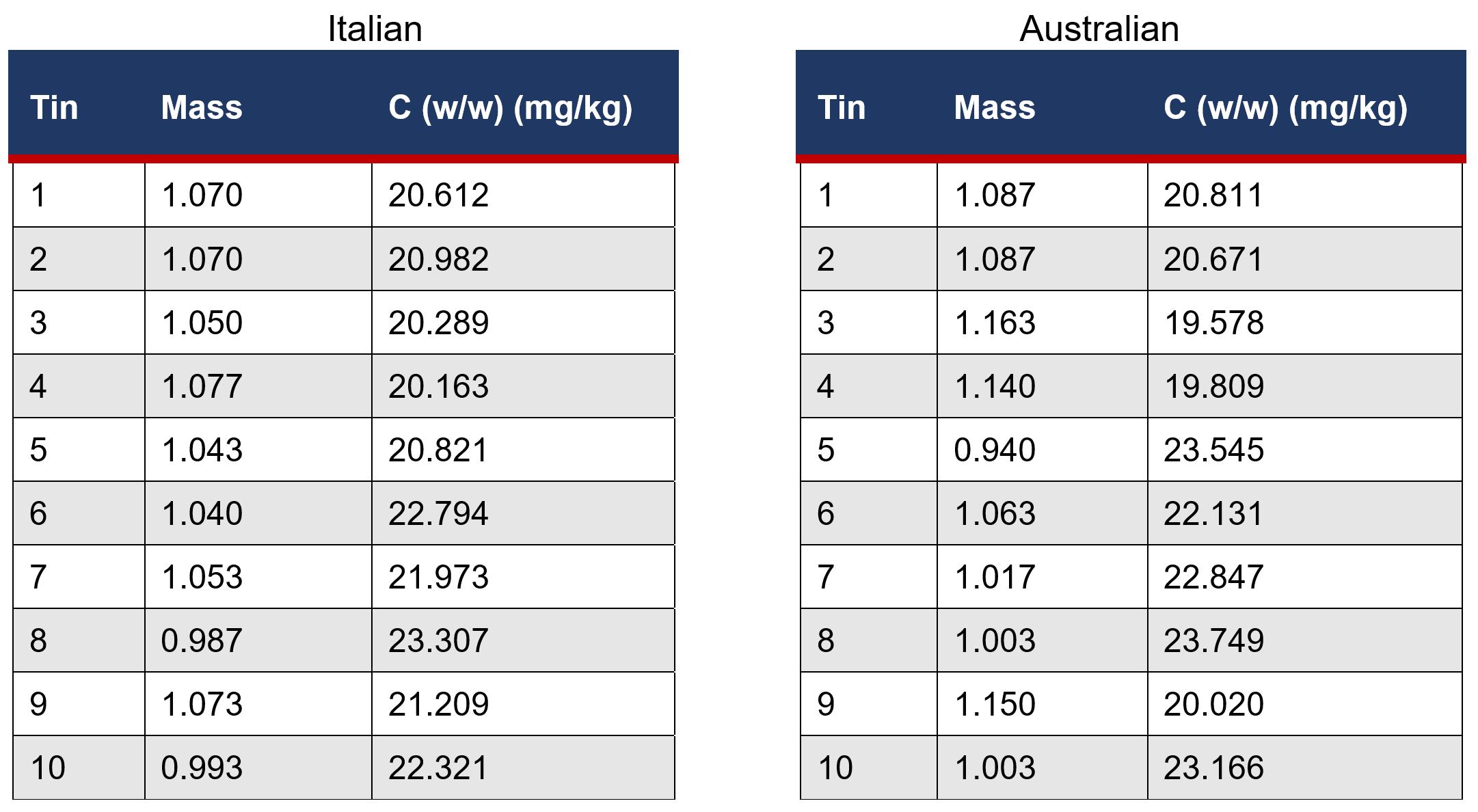
Australian Italian Mean 21.6326138 21.4472161 Variance 2.66230031 1.185041446 Observations 10 10 df 9 9 F 2.24658835 P(F<=f) one-tail 0.12184245 F Critical one-tail 3.1788931
The Journal of Science Extension Research – Vol. 2, 2023 education.nsw.edu.au 153
Data after calculation of concentration and removal of outliers
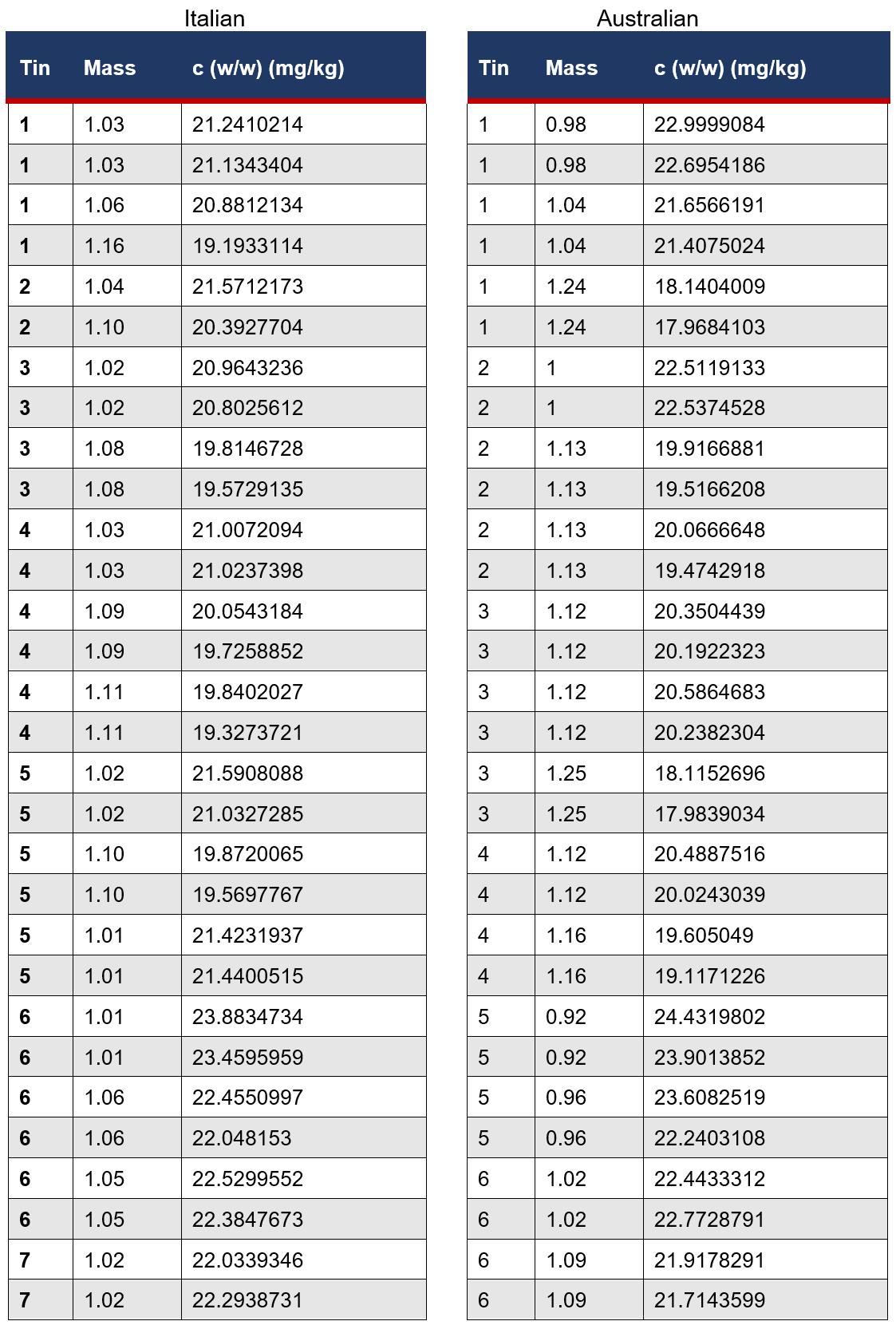
The Journal of Science Extension Research – Vol. 2, 2023 education.nsw.edu.au 154
The Journal of Science Extension Research – Vol. 2, 2023 education.nsw.edu.au 155
Image of absorbance of the top layer of solution showing the slight inaccuracy in the software.
How The Anomalous Behaviour of Hydrogen Fluoride Provides Insight Into The Nature of Ionisation
Theo Mortazavi
Normanhurst Boys High School
The anomaly behind the weak acid nature of hydrofluoric acid has sparked scientific discourse for nearly a century, with the most recent explanation accounting a lack of ionisation to entropic factors. This report extrapolates the theorised principle by establishing causation between hydration entropy of a wide array of monoprotic acid anions and their tendency to ionise in an aqueous system. Entropic data was obtained through the CHSNOZ package of freely available RGUI software, plotted against ionisation tendency compiled by IUPAC handbooks, and regression was tested. Ultimately it was found that an increased hydration entropy of monoprotic anions is directly related to a decreased tendency of the acid to ionise in an aqueous solution
1. Literature Review 1
1.1 Advancement of Hydrofluoric Acid Theory
Despite its relative abundancy, Hydrofluoric acid it remains an anomaly amongst hydrohalic acids given its classification as a Brønsted-Lowry weak acid where, formerly, a weak acid is classified as one with a pKa value greater than a Hydronium ion. (pKa ≥ -1.74)
higher net polarity would increase bond stability and decrease ionisation tendency. While this holds true amongst the Hydrohalic acids, the inverse trend is observed across the period, undermining the validity of Pauling’s conclusions.
1.1.1 Linus Pauling
This superficially simple outlier gained notary after Nobel Prize Laureate Linus Pauling’s paper on the matter. 3 Pauling theorised that electronegativity of the halogen determined the acidity, where a
1 Record of Collaboration included in S.1.2 portfolio.
2 Equation (1) shows the partial ionisation of hydrofluoric acid, indicated by the equilibrium arrow
3 L. Pauling, ‘Why is Hydrogen Fluoride a weak acid? An answer based on a correlation of free energies with electronegativities’ Journal of Chemical Education, vol 33, no. 1, 1956, pg. 16-17
4 Table 1 quantifies the relationships between pKa and electronegative amongst hydrohalic acids
��������(��������) + ����2 ����(���� ) ⇋ ����3 ����(��������) + +����(��������) (1) 2
Table 1 4
The Journal of Science Extension Research – Vol. 2, 2023 education.nsw.edu.au 156
1.1.2 Giguere and Turrel
Giguère and Turrel, instead theorised that HF did in fact completely (or largely) ionise into H3O+(aq) and F-(aq) bound complexes, hence still acting as a weak acid. 6 These complexes would appear as H3O+(aq) band on an infra-red spectrum, however, would account for the low recorded pH of HF, hence explain the apparent lack of ionisation, given;
H3O+ ions as opposed to classically bound HF. Given the absence of repeated trials with appropriate spectroscopic evidence, this report bore largely unreliable conclusions.
1.1.3 Ayotte Herbert and Marchland
Ayotte, Hèrbert and Marchland contradicted these findings through analysis of the Born-Haber cycle, which describes the various enthalpy (H) pathways for the ionisation of HF. 7
For:
Where:
However, this controversial conclusion has been met with criticism given the absence of suitable spectroscopic crossreferencing, where the IR spectra alone insufficiently confirms the presence of

Figure 1 8
As seen in Figure 1, while there is a substantial (+) homolytic bond enthalpy from gaseous HF to H▪ and F▪ radicals, the hydration enthalpy (ΔH) releases almost equal energy, resulting in a net exothermic reaction, which should favour ionisation via Standard state free energy principles. 9 Yet via the Gibb’s Free Energy equation, the ionisation of HF
5 Table 2 quantifies the relationship between pKa and electronegativity across period 2 compounds
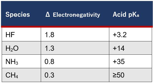
6 P. Giguere and S. Turrell, ‘The Nature of Hydrofluoric Acid. A Spectroscopic Study of the Proton-Transfer Complex H3O+▪F-‘Journal of the American Chemistry Society, vol. 102 no 1, 1980, pg. 5473
7 P. Ayotte, M Herbert and P. Marchland, ‘Why is hydrofluoric acid a weak acid?’, The Journal of Chemical Physics, vol. 123, no. 1, 2005, pg. 2
8 Figure 1 shows the Born-Haber cycle of HF on an energy profile diagram, with data transformed from the report of Ayotte, Hèrbert and Marchland
9 P. Ayotte, M Herbert and P. Marchland, ‘Why is hydrofluoric acid a weak acid?’, The Journal of Chemical Physics, vol. 123, no. 1, 2005, pg. 2
Table 2 5
��������(��������) + ����2 ����(����) ⇋ ����3 ����(��������) + +����(��������) (3)
The Journal of Science Extension Research – Vol. 2, 2023 education.nsw.edu.au 157
yields an endergonic dissolution. (Δ����° = +3.2kJmol-1) 10
The Ka (acid dissociation constant) can be directly related to the entropy ΔS, with respect to ΔH.
of value. Therefore, the most practical and potentially rewarding avenue of research will limit the scope of this report to establishing causation between hydration entropy and ionisation tendency.
2.1.1 Justification
They concluded that the (+) ΔG value must be a direct implication of a larger ΔS value which was due to the larger negative hydration entropy of the fluoride ion, compared to the larger Chloride, Bromide and Iodide ions. According to subsequent works of T.Joutsuka and K. Ando, these larger ions less prominently disrupted hydrogen bonding networks, lessening the change in entropy. 11 Therefore, it was concluded that HF acts as a weak acid in water due largely due to the entropy of hydration.
2.1 Research Gaps and Evaluation of Scope
While there has been a relative consensus reached on the causation of HF as a weak acid, this anomaly poses wider questions towards the generalised relationship between ionisation and hydration entropy for monoprotic acids. Given that substantive literature explaining the relationship between acid strength and concentration, as well as ionisation tendency and nonentropic thermochemical measures, further investigation into these well-established relationships would yield little conclusion
The literature review suggests existing complexities in establishing relationship between ionisation and entropy of HF, hence this report will only cater to monoprotic acids, given that Polyprotonation introduces equilibrium calculations which introduce further variables.
Moreover, pKa will be used as the sole measure of ionisation within this report, given that Ka produces values with greater variance, leading to unnecessary complications in statistical processing. pH is equally rejected given its greater temperature dependence and variation due to experimental conditions, increasing the chance of systematic and random error which could reasonably compromise the internal validity of this report.
3.1 Scientific Research Question
Whether hydration entropy of monoprotic acid anions affect their ionisation tendency within an aqueous solution.
4.1 Null Hypothesis (H0)
That hydration entropy of the monoprotic acid anion in aqueous solution does not affect its ionisation tendency.
10 P. Ayotte, M Herbert and P. Marchland, ‘Why is hydrofluoric acid a weak acid?’, The Journal of Chemical Physics, vol. 123, no. 1, 2005, pg. 1
11 T. Joutsuka and K. Ando, ‘Hydration Structure in Dilute Hydrofluoric Acid’ The Journal of Physical Chemistry, vol. 115, no. 1, pg. 671-67
��������ℎ��������
��������ℎ�������� ∘ =
∘ −������������ℎ�������� ∘ (5)
��������ℎ�������� ∘
��������ℎ�������� ∘ ���� + ���� ln(�������� ) (6)
=
The Journal of Science Extension Research – Vol. 2, 2023 education.nsw.edu.au 158
4.2 Alternate Hypothesis (Ha)
That a lower absolute hydration entropy of monoprotic acid anion in aqueous solution increases its ionisation tendency.
5.1 Evaluation of Experimental Design and Risk Assessment
Data collected for the methodology was purely secondary, given the lack of access to instruments which would give readings of acceptable accuracy, and the inherent risks associated with working with corrosive acids. Therefore, data was instead sourced from reputable secondary sources, conducted in highly controlled conditions, with acutely accurate instrumentations, producing a valid and scrutinised set of results.
To gather these data sources, Google Scholar was used to narrow down reports which may have included a relevant dataset, using keywords such as ‘hydration entropy’ and ‘pKa dataset.’ After a relevant report was identified, the experimental data was crosschecked with theoretical data, to gauge the degree of accuracy. The data source was then further examined, assessing whether the paper and journal are peer-reviewed, as well as how many publications the author(s) had. Finally, citations of this source were checked, where less sources did not necessarily indicate an invalid source, it did infer that the data is less peer-reviewed. However, if citations were found to be of a high quality, even in few, the dataset was considered reliable and
valid enough for the purposes of this report. This process was repeated to increase the size and breadth of the dataset, maintaining a standard of reliability and validity of the results.
Inorganic data collection relied upon publicly available datasets including the National Institute of Standards and Technology (2021) [NIST], which were both used to cross-reference experimental values obtained by research reports. 12Data pertaining to the thermochemistry of anion hydration including ΔS was gathered by the experimental reports where available data was cross-referenced with the NSIT, while data pertaining to the experimentally calculated pKa was collected solely from peer reviewed databases including IUPAC, in doing so, increasing the number of sources and datapoints which optimises reliability and contributes towards internal validity. 13 14
After collecting the inorganic data values, it became apparent there was insufficient homologous data to establish a correlation between pKa and ΔS, hence data was gathered from organic values with extensive aliphatic homologous series. To maintain internal validity within the procedure, only monoprotic carboxylic acid and 2-hydroxycarboxylic acid series were collated, with IUPAC published handbooks used to gather pKa values at 298.15K, cross-referenced with the National Library of Medicine PubChem Database, to ensure reliability. 15
12 National Institute of Standards and Technology, ‘NIST Chemistry Webbook,’ 2022 https://webbook.nist.gov/chemistry/ Accessed 21st August 2022
13 Y. Marcus, ‘The hydration entropies of ions and their effects on the structure of water,’ J. Chem. Soc., Faraday Trans. 1, 1986,82, 233-242
14 A. M. Slater, ‘The IUPAC aqueous and non-aqueous experimental pKa data repositories of organic acids and bases’ Comput Aided Mol Des. 2014 Oct;28(10):1031-4. Pg. 1-4
15 Pubchem
The Journal of Science Extension Research – Vol. 2, 2023 education.nsw.edu.au 159
The CHNOSZ database was accessed via the RGUI software was the only viable database of organic entropy values pertaining to each homologue at 298.15K, within a sophisticated coding framework. (detailed in the appendix) 16 17
Inorganic and Organic data was ultimately tabulated and graphed, with respect to the homologous series, with regression values independently calculated through Microsoft Excel for each dataset, based on a highly valid experimental procedure.
5.2 Considerations of Accuracy
Given the accurate nature of this report, only databases which used highly accurate data were
included. Experimental data pertaining to calculations of pKa creates systematic inaccuracies, given the often insignificant [A-] in solution for weak acids and [HA-] for strong acids.
McTigue, O’Donnell and Verity addressed this accuracy by comparing registered the calculated molarity of HF solutions by both potentiometric and conductometric quantitative analysis technology. 18 They found that for 0.5molal (m) and 1.0m solutions of HF, the above methods were accurate. However, for concentrations approaching 6m, accurate readings required comparison of activity coefficients in the Debye-Huckel Equation.
Extended Debye-Huckel Equation (general form):
Derived Debye-Huckel Equation
19
��������
While for strong acids, an uncontrollable degree of uncertainty exists given the negligible residual [HA], accuracy can be maximised through calculations using the Hammet acidity function.
Similarly, by using RGUI software and NIST database for all thermochemical data, peer-reviewed and highly accurate calculations are used to map entropy values to various stages of the BornHaber cycle. By using these specific entropy values rather than net entropic considerations, this report is able to accurately relate the hydration entropy of the anion to ionisation tendency and optimise accurate data within this report.
16 J. M. Dick, ‘An Introduction into CHNOSZ,’ 2022, https://cran.rproject. org/web/packages/CHNOSZ/vignettes/anintro.html#installing-and-loading-chnosz
17 Specific methodology referenced in the appendix
18 P. McTigue, T. O’Donnell and B. Verity, ‘The determination of Fluoride Ion Activities in Moderately Concentrated Aqueous Hydrogen Fluoride’, The Australian Journal of Chemistry, vol. 38, no. 1, 1985, pg.1798, 1803.
19 ���� = activity constant, A and B are universal constants: A = 0.5085, B = 0.3281, z is the integer charge of the ion, I is the ionic strength on the molal scale and b is the adjustable parameter: bHF = 0.2
(���� )= ����|���� ����+ |√���� 1+��������√���� (7)
������������
(������������ )= −������������ ���� (8)
The Journal of Science Extension Research – Vol. 2, 2023 education.nsw.edu.au 160
6. Results
6.1 Inorganic pKa vs ΔS values
Results table 1 shows the cross referenced pKa values of inorganic anions dependent on their hydration entropy.
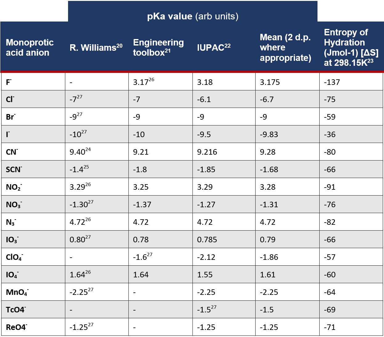
The Journal of Science Extension Research – Vol. 2, 2023 education.nsw.edu.au 161
Results table 3 shows Excel calculated regression confidence testing for all inorganic datapoints
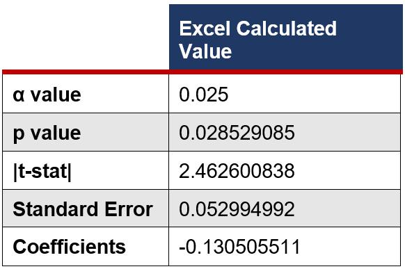
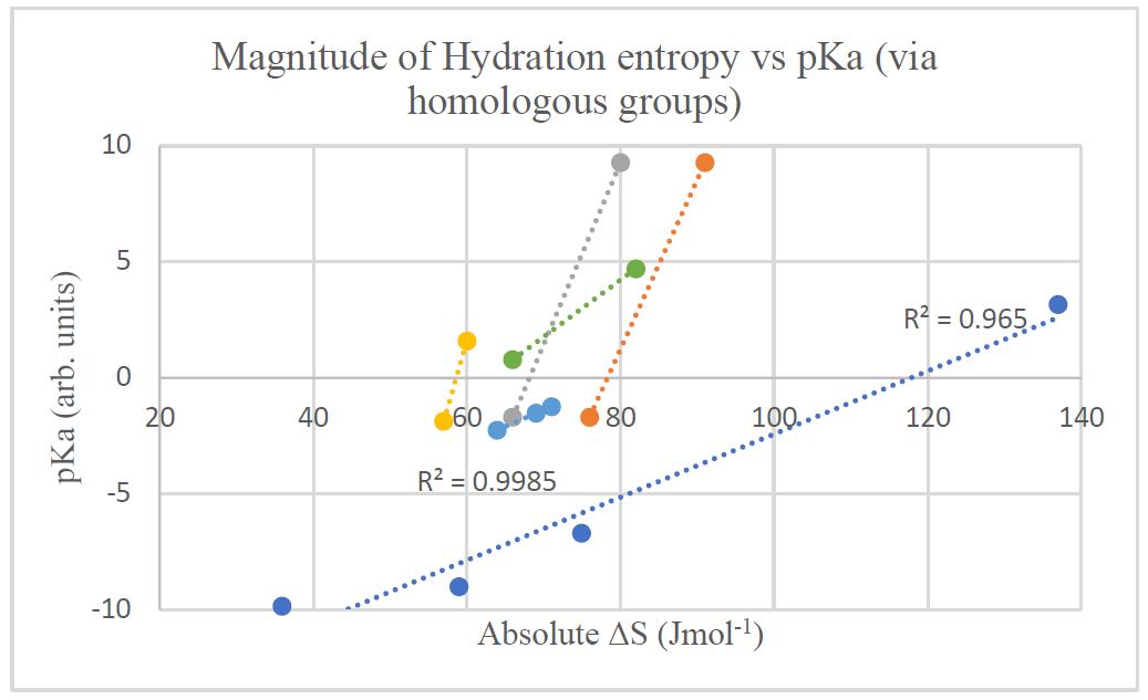
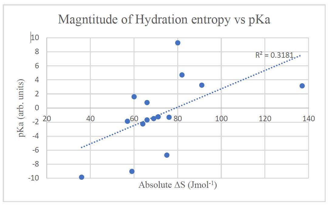 Graph 1 shows ΔS against pKa without respect to homologous series.
Graph 2 shows the correlation between ΔS and pKa within respect to each inorganic homologous series, where only the hydrohalic acids had enough datapoints to draw an informed R2 value.
Graph 1 shows ΔS against pKa without respect to homologous series.
Graph 2 shows the correlation between ΔS and pKa within respect to each inorganic homologous series, where only the hydrohalic acids had enough datapoints to draw an informed R2 value.
The Journal of Science Extension Research – Vol. 2, 2023 education.nsw.edu.au 162
6.2 Organic pKa vs ΔS Results table 4 shows the first sixteen aliphatic, carboxylic acid anions with their pKa gathered from IUPAC/PubChem and entropy values obtained through the CHSNOZ database accessed via the RGUI software. 202122
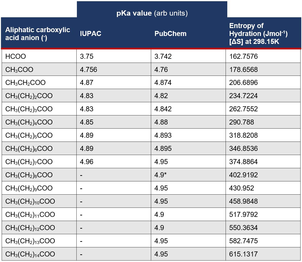
20 A. M. Slater, ‘The IUPAC aqueous and non-aqueous experimental pKa data repositories of organic acids and bases’ Comput Aided Mol Des. 2014 Oct;28(10):1031-4.
21 National Center for Biotechnology Information (2022). PubChem Compound Summary for CID 11005, Myristic acid. Retrieved August 21, 2022 from https://pubchem.ncbi.nlm.nih.gov/compound/Myristic-acid.
22 J. M. Dick, ‘An Introduction into CHNOSZ,’ 2022, https://cran.rproject. org/web/packages/CHNOSZ/vignettes/anintro.html#installing-and-loading-chnosz
The Journal of Science Extension Research – Vol. 2, 2023 education.nsw.edu.au 163
Results table 5 shows the aliphatic, 2-hydroxycarboxllic acid’s, collated an eidetic manner.
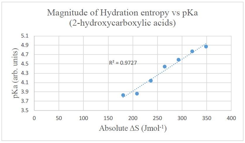
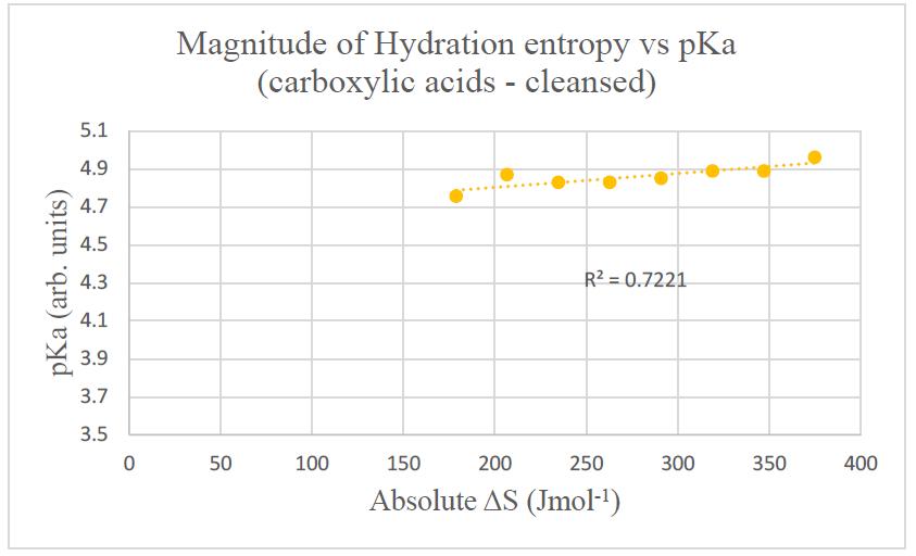
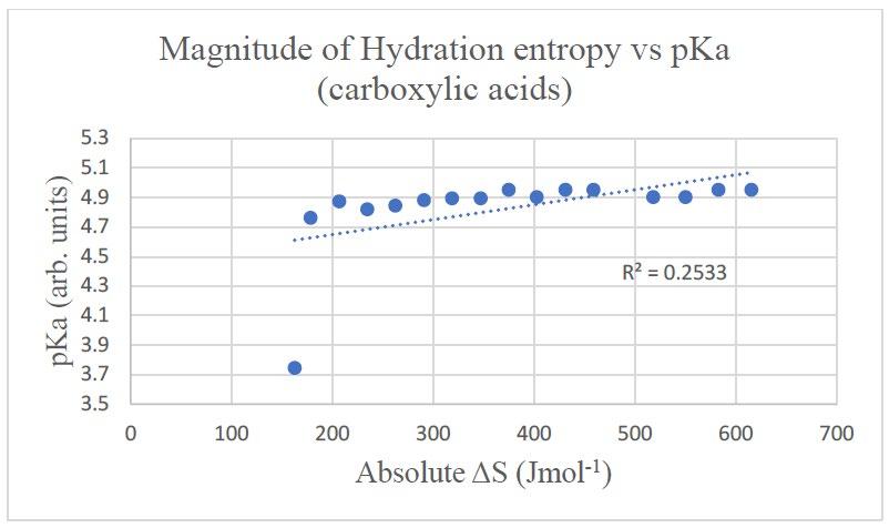
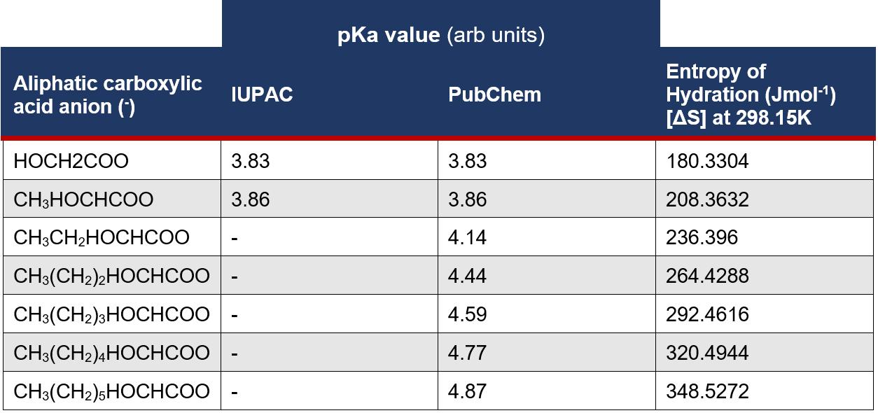
6.2.2 Regression Confidence Testing
Results table 6 shows Excel calculated regression confidence testing for the organic datapoints.
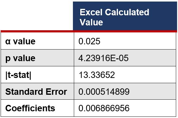 Graphs 3 displays the uncleansed data collected in Results table 4.
Graph 4 displays the cleansed version of data collated in Graph 3 as explained in discussion.
Graph 5 displays the uncleansed data collected in Results table 5
Graphs 3 displays the uncleansed data collected in Results table 4.
Graph 4 displays the cleansed version of data collated in Graph 3 as explained in discussion.
Graph 5 displays the uncleansed data collected in Results table 5
The Journal of Science Extension Research – Vol. 2, 2023 education.nsw.edu.au 164
7.1 Inorganic Correlation
The inorganic data presented several problems which was reflected in the statistical analysis and undoubtedly related to a lack of consistent data, leading to complexities in analysing trends. In plotting all inorganic datapoints within a single scatterplot, the R2 coefficient showed that only 31.18% of data could be explained by the line of best fit, showcasing a moderate (+) Pearson coefficient of 0.564 indicating that an increase in ΔS was only weakly related to a general increase in pKa
However, this result was reasonably expected given the innate difference in chemical properties between homologous series, yet, there was little that could be done to mitigate these limitations.
Namely, there existed a lack of datapoints given an intrinsic lack of homologues within a period or group. For instance, despite gathering conclusive date for the complete homologous series of hydrohalic acids, given that only four homologues exist, there exists a limitation on the strength of causation as opposed to spurious correlation. Therefore, even despite yielding an R2 coefficient where 95.6% of data could be explained by the line of best fit (as seen in graph 2), to consider this limited dataset as a confirmation of my alternate hypothesis would present ethical implications which could reasonably compromise the internal validity of this report. This issue could not simply be rectified by a modification of experimental method, given that the raw values of pKa and ΔS of hydrohalic acids
cannot be accurately, nor validly compared to those of any other homologous series without compromising controlled variables. Namely, differences in atomic radius alter thermochemical properties, while polarity and electronegativity distribution variations between homologous series render raw pKa and ΔS incomparable and such comparison would compromise controls and the validity of the trend. 23
7.2 Inorganic Statistical Analysis
Despite the limited success in establishing a correlation coefficient, the regression confidence statistics found a p-value of 0.0285 (3sf) which despite being above the threshold one-tailed α value of 0.025 still indicates that the chance of the data randomly taking on this distribution is only 2.85%, seen in results table 3. While it is still imperative to reject the alternative hypothesis on this account to maintain an unbiased report, the relatively low standard error value of 5.23% (3sf) indicated that a larger, consistent dataset such as organic homologues would provide statistically supported results.
7.3 Organic Correlation
The use of homologous, carboxylic acids provided substantial and confident correlation between the hydration entropy and pKa. Given that aliphatic carboxylic acids vary between homologues based on the addition of a -CH2- methylene bridge rather than element in a group, the limitations seen in the inorganic dataset,
7 Discussion
23
J.
1991, 87(18), 29952999 The Journal of Science Extension Research – Vol. 2, 2023 education.nsw.edu.au 165
Y. Marcus, ‘Thermodynamics of solvation ions,’
CHEM. SOC. FARADAY TRANS.,
in this respect, were vastly overcome. 24 Aliphatic carboxylic acids are justifiable choices of dataset given they are monoprotic and weak acids, proving substantial chemical similarity to the inorganic acids, moreover, by not directly comparing entropy or pKa values with the inorganic datapoints, any variations are eliminated, where the line of best fit uses the marginal increase of values rather than the absolute value. 25 Furthermore, the substantial size and accuracy of the data available through the RGUI software greatly increased the validity of any trend established, where the CHNOS Z calculations provided entropy values to 7 significant figures with an uncertainty below ±10-4 %.
However, Results table 4 and graph 3 showcase that even despite the increase in the number of data entries, there is still only moderate positive correlation of 0.5032 with only 25.33% of data being explained by the line of best fit. Yet the cleansed data presented in graph 4 provide a high correlation value of 0.8498 with 72.21% of variance data explained. The variation in these values was attributed to the data cleansing process which limited the dataset to decanoic acid and removed only a single data entry of methanoic acid, which has a pKa of 3.83 and a hydration entropy of 180Jmol-1
This was justifiable given that while there is no significant anomaly within the entropy value, the pKa indicated that methanoic acid has a tendency to ionise more than ten times greater than its subsequent ethyl homologue. Given that the IQR of the dataset is 0.104, and the 3.83 value lies 9.79 (3sf) standard deviations below Q1, it can be considered an extreme outlier and validly excluded. 26 In terms of principle, methanoic acid exhibits this significantly higher ionisation tendency given its higher net polarity than subsequent homologues, as well as a lower molar mass, which biases its tendency to form strong hydrogen bonding lattices over dispersion forces seen within the longer carboxylic acids, hence given its anomalous behaviour there are few disadvantages from its exclusion, however, significant improvements in improving correlation. 27 In terms of cleansing carboxylic acids with a chain length greater than decanoic acid are biased so heavily towards dispersion forces that their aqueous solubility is reduced to the degree that pKa results are no longer accurate, explaining the stagnant and illogical fluctuations between 4.9 and 4.95 for these acids that is seen in results table 4 28
24 J. Holmes, T. Jean, ‘The mass spectra of carboxylic acids–II: Fragmentation mechanisms in the homologous series HOOC(CH2)nCOOH’ Journal of Mass Spectrometry Volume 3 Issue 12 1970
25 A, Alwash. ‘Carboxyllic acid: Nomenclature, preparation, physical properties, and chemical reactions,’ 10.13140/RG.2.2.16402.48326. 2022 pg1-6
26 Ref. to appendix item 4
27 G, Torsten, K, Holger, K. Volker, R., Andreas K, Udo. (2018). Carboxylic acids in aqueous solutions: Hydrogen bonds, hydrophobic effects, concentration fluctuations, ionization, and catalysis. The Journal of Chemical Physics. 149. 244503. 10.1063/1.5063877. pg 2
28 G, Torsten, K, Holger, K. Volker, R., Andreas K, Udo. (2018). Carboxylic acids in aqueous solutions: Hydrogen bonds, hydrophobic effects, concentration fluctuations, ionization, and catalysis. The Journal of Chemical Physics. 149. 244503. 10.1063/1.5063877. pg 3
The Journal of Science Extension Research – Vol. 2, 2023 education.nsw.edu.au 166
Ultimately, the most successful correlation came from analysis of the 2hydroxycarboxylic acid homologous series, where the uncleansed dataset provided a Pearson’s correlation coefficient of 0.986, which is a strong, positive correlation, with 97.27% of data explained by the line. Given that these homologues bear similarity to both the aliphatic n-carboxylic acids without the limitation imposed by the low aqueous solubility, accurate measures of pKa were collated against the same highly accurate calculations of hydration entropy, decreasing the uncertainty of the dataset. Notably, the addition of the alcohol functional group at Carbon position 2 led to an average decrease in pKa between the 2-hydroxycarboxyllic acid and its ncarboxylic acid alkyl counterpart, however, an systemically increased ΔS value (results table 5). These two trends can be justifiably attributed to the increased polarity of the OH group, which given a higher atomic radius, equally increases the solvation entropy. 29
7.4 Organic statistical analysis
In considering the regression statistical testing for the organic data, the calculated p value of 4.24E-5 is significantly lower than the alpha value of 0.025, indicating that there is statistical significance to the correlation (results table 6). In such case, the null hypothesis may be rejected and the alternate hypothesis accepted given that the organic data isolates a more valid causal relationship between hydration entropy and pKa than the inorganic data, by controlling more
variables. Perhaps more interestingly is the apparent negligibility of the identified coefficient of 0.00687 (3sf) which suggests that the increase in pKa is low compared to the increase in ΔS. While this could reasonably be construed to suggest that the ΔS is a negligible influence on pKa, this would be an invalid conclusion given that pKa is a logarithmic scale hence is expected to showcase a smaller absolute increase. The extremely lows standard error at approximately 1/13th of the coefficient indicates a lower spread of the data given that the residual of each datapoint is negligible, indicating a higher confidence interval in the sample.
8. Conclusion 30
Ultimately, this study substantiates the relationship between hydration entropy of monoprotic acid anions and the tendency of the acid to ionise in solution. While this study was able to effectively isolate the correlation in this trend in the case of specific homologous series, it lacked the facilities and resources to extend this relationship definitively, or to specifically consolidate a relationship for HF. While it established a direct proportionality between hydration entropy and pKa it failed to quantitively derive this relationship amongst all aqueous systems.
Given the scope of this research and its societal and research implications, there are an array of necessary directions to further the understanding on the relationship between entropy and
29 G, Torsten, K, Holger, K. Volker, R., Andreas K, Udo. (2018). Carboxylic acids in aqueous solutions: Hydrogen bonds, hydrophobic effects, concentration fluctuations, ionization, and catalysis. The Journal of Chemical Physics. 149. 244503. 10.1063/1.5063877. pg 5-6
30 Record of Peer Review in S.3.1 Of Portfolio
The Journal of Science Extension Research – Vol. 2, 2023 education.nsw.edu.au 167
ionisation. Namely, to bias the thermochemical influence on pKa away from enthalpy and towards entropy, experimental data could be gathered in pseudo-aqueous systems at cryogenic temperatures. To calculate the pKa at these temperatures, the highest degree of accuracy could be obtained by using computer models, similar to those used in the RGUI programming for ΔS values. From this, the temperature dependence of pKa on ΔS could be established, which would innately consolidate the proportionality established in this report.
References
1. ACS, ‘Molecule of the week archive: Hydrogen Fluoride’ ACS, 2021, pg. 1 https://www.acs.org/content/acs/en/molec ule-of-theweek/archive/h/hydrogenfluoride.html
2. A, Alwash. ‘Carboxyllic acid: Nomenclature, preparation, physical properties, and chemical reactions,’ 10.13140/RG.2.2.16402.48326. 2022
pg1-6
3. Ayotte, P, Herbert, M. and Marchland, P., ‘Why is hydrofluoric acid a weak acid?’, The Journal of Chemical Physics, vol. 123, no. 1, 2005, pg. 1-8
4. Dick, J. M. ‘An Introduction into CHNOSZ,’ 2022, https://cran.rproject.org/web/packages/C HNOSZ/vignettes/anintro.html#installingand-loadingchnosz
5. Giguere, P. and Turrell, S. ‘The Nature of Hydrofluoric Acid. A Spectroscopic Study of the Proton-Transfer Complex H3O+▪F-‘, Journal of the American Chemistry Society, vol. 102 no 1, 1980, pg. 5473-5477
6. Holmes, J. Jean, T. ‘The mass spectra of carboxylic acids–II: Fragmentation mechanisms in the homologous series HOOC(CH2)nCOOH’ Journal of Mass Spectrometry, 1970 , Volume 3 Issue 12
7. Joutsuka, T. and Ando, K. ‘Hydration Structure in Dilute Hydrofluoric Acid’ The Journal of Physical Chemistry, vol. 115, no. 1, pg. 671-677
8. Marcus, Y. ‘Thermodynamics of solvation ions,’ J. CHEM. SOC.
FARADAY TRANS., 1991, 87(18), 29952999
9. Y. Marcus, ‘The hydration entropies of ions and their effects on the structure of water,’ J. Chem. Soc., Faraday Trans. 1, 1986,82, 233-242
10. McTigue, P. O’Donnell T. and Verity, B. ‘The determination of Fluoride Ion Activities in Moderately Concentrated Aqueous Hydrogen Fluoride’, The Australian Journal of Chemistry, vol. 38, no. 1, 1985, pg.1798-1807
11. National Centre for Biotechnology Information (2022). PubChem Compound Summary for CID 11005, Myristic acid. Retrieved August 21, 2022 from https://pubchem.ncbi.nlm.nih.gov/compou nd/Myristic-acid.
12. National Industrial Chemicals Notification Scheme, ‘Hydrofluoric acid (HF)’ NICNS, 2001, pg. 1-128, https://www.industrialchemicals.gov.au/sit es/default/files/PEC19-Hydrofluoricacid.pdf
13. National Institute of Standards and Technology, ‘NIST Chemistry Webbook,’ 2022 https://webbook.nist.gov/chemistry/ Accessed 21st August 2022
The Journal of Science Extension Research – Vol. 2, 2023 education.nsw.edu.au 168
14. Pauling, L. ‘Why is Hydrogen Fluoride a weak acid? An answer based on a correlation of free energies with electronegativities’ Journal of Chemical Education, vol 33, no. 1, 1956, pg. 16-17
15. Simons, J.H. ‘Hydrogen Fluoride Catalysts’ Advances in Catalysts, vol.2, no.1 pg. 197-232
16. Torsten, G. Holger, K Volker, W. Andreas, R. Udo, K. ‘Carboxylic acids in aqueous solutions: Hydrogen bonds, hydrophobic effects, concentration fluctuations, ionization, and catalysis. The Journal of Chemical Physics.’ 2018, 149. 244503. 10.1063/1.5063877.
17. The Essential Chemical Industry, ‘Hydrogen Fluoride’ The Essential Chemical Industry-Online, 2017 pg. 1 ‘https://essentialchemicalindustry.org/che micals/hydrogen-fluoride.html’
18. Williams, R. ‘pKa data compiled by R. Williams,’ American Chemical Society, Organic Division vol 23, no.1 updated 2022 pg1-5
Acknowledgements
Undertaking this research project was equally difficult and rewarding, often garnering sardonic reactions from my non-scientific peers as they see my countless pages of seemingly nonsensical numbers. However, with the support from various key sources, this report has transformed from a simple assignment to a personal passion, with a bittersweet ending. Without doubt, my teacher supervisor, Ms Ritu Bhamra has been at centre of my support and assistance, whether it was conceptualising my research idea, fleshing it out into a practical methodology and especially answering
my last-minute question, saving me from unwavering deadlines.
Moreover, my peers in the class as whole, especially Babu and Evan, have been foundational in balancing my extreme ideas with reasonable pragmatism and insightful approaches to my problems. Without their contribution I would likely still be pulling my hair out while trying to perform complex solvation calculations on non-aqueous solvents, or singing my fingertips with highly corrosive acids.
Externally, I would like to thank Professor Robbie Girling at the University of Reading for his contributions into the process of writing a scientific report and Jacob Marlow in providing me the theoretical insight into thermochemistry, which I would otherwise be lost without.
Finally, I would like to thank my fellow year 12 student, Alec Peng. Alec is unintentionally responsible for this report as a whole, given that my scientific premise was derived from one of his superficially simple questions in Chemistry class last year that I was simply unable to answer. Until now that is.
What is striking now that I have concluded this 9-month project is the shift in perspective it has offered me. In first endeavouring on this project, I was ambitious in trying to disprove complex particle physics, yet now having gained closure to a far simpler, but personal scientific query, I have found an immense satisfaction.
Appendix:
CHSNOZ coding:
The Journal of Science Extension Research – Vol. 2, 2023 education.nsw.edu.au 169
Acid search was available through the command info(“acid”) from which 20 aliphatic ncarboxylic acids were available and 10 2-hydroxycarboxyllic acids.

31Specific thermochemical data, including ΔS, was gathered by gathering the unique identifier code result from the first
Appendix Item 1:
info(“acid”) display function:
command and performing the subcrt(“”) command 32. From this, tabular ΔS was displayed as a function of temperature, where only the value pertaining to 298.15K was obtained as to control temperature variable with respect to the pKa. 33
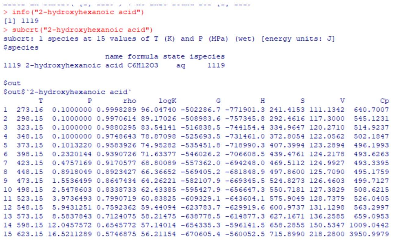
Appendix item 2:
Subcrt(“”) display function
Appendix item 3: units function
31 Ref to appendix item 1
32 Ref to appendix item 2
33 To ensure that this data was gathered in uniform units, the command E.units (“J”) and T.units (“K”) pre-set all calculations to degrees Kelvin and Jmol-1.
The Journal of Science Extension Research – Vol. 2, 2023 education.nsw.edu.au 170
Appendix item 4:

Boxplot pertaining to the data cleansing of methanoic acid as an outlier – note the pKa value of methanoic acid is displayed beyond the 4.5 lower bound of the boxplot at 3.742
Appendix item 5:
The Journal of Science Extension Research – Vol. 2, 2023 education.nsw.edu.au 171
Plant Power vs the Water World: An Insight into the Detoxifying Properties of Typha Orientalis in Polluted Water.
Elena Mbeya
Menai High School
Abstract
This investigation explored the detoxifying and filtrating properties of Typha Orientalis, a wetland plant, in the removal of Copper (II) Sulfate and Cooking Oil in water – to simulate pollutants found in Sydney Harbour. As per data provided by Gavin Birch and the School of Geosciences at the University of Sydney. This experiment, carried out over the course of 43 days (29/06/2022 – 11/08/2022), provided quantitative and qualitative data to support the application of Typha Orientalis in the filtration of polluted water in the real world, ultimately to reach a safe level of contaminants fit for consumption as deemed by World Health Organisation. Although a communication error was encountered with the exact measurements of Copper (II) Sulfate and Cooking Oil, the results showed an average 68.75% decrease of Cooking Oil in a 100mL sample, measured through sedimentation, and an average 15.57% increase in ‘B’ on the RGB scale in 10mL samples, measured through copper test strips and a colour identification app ‘What Colour Is this’, by Nicholas Troia, indicating a 15.57% decrease in Copper (II) Sulfate, supported through data analysis. The descriptive statistics from each sample yielded a Pvalue<0.0001, resulting in >99.99% statistical significance in the difference in data sets, rejecting the null hypothesis and accepting the alternate hypothesis with strong statistical evidence.
Literature Review
Water pollution has become one of our planet’s greatest environmental problems, leading to things such as coral bleaching and ocean warming. (Do, W., & Jamerson, M., 2021). Ingesting contaminated water can lead to diseases such as cholera, dysentery, typhoid, and polio which in most cases lead to death. 850 million people globally don’t have access to clean drinking water, and this subsequently kills one person every 10 seconds. (Cassoobhoy, A. 2020). Due to the inconsistent data surrounding the
treatment of wastewater, there was a need to investigate this issue, driven by social and environmental needs.
Scientists at the College of Forestry, Beijing Forestry University, have extensively researched the capacity of aquatic plants to absorb heavy metals in polluted water. Their analysis aided in identifying the selection of aquatic plants that are suitable for heavy metal absorption from real life polluted waters. They provided quantitative data supporting plants from the Gramineae, Pontederiaceae, Ceratophyllaceae, Typhaceae and Haloragaceae and their
The Journal of Science Extension Research – Vol. 2, 2023 education.nsw.edu.au 172
relatively strong abilities to absorb these metals. However, the absorption abilities varied with the plant organ, with the following trend: roots > stems > leaves, establishing a hierarchy within this set group of plants, meaning the plants that absorb nutrients/water through their roots would be more effective in the detoxification and filtration of polluted water. (Li, J., Yu, H., & Luan, Y., 2015). This selection reduced the large array of aquatic plants that could be used in this investigation, refining the research, but lacked information on specific plants, within the families, that were the most effective.
After a review of aquatic plants that are easily sourced, non-invasive and fit within the 5 families outlined above, bulrushes were the most appropriate (Gardening With Angus Bringing You the Best In Australian Plants And Gardening, n.d.). In an interview conducted by (Sahtouris, E, 1990), Kathe Siedel outlines how she collated different sets of data collected by different scientists and combined them to create one meta-analysis that addressed all areas in bulrushes capabilities,
investigating the phenomenon in a realworld environment, meaning there was minimal control over different variables but showed the extent of the plants capabilities in harsh environments, much like the Scientists at the College of Forestry, Beijing Forestry University. Although she highlights that bulrushes can work all year round (Sahtouris, E,. 1990), in winter the bulrushes prepare to partially die off before producing new life in spring, going dormant (Gardening With Angus Bringing You the Best In Australian Plants And Gardening, n.d.), the extent of Kathe Seidel’s investigation had identified that dead or even harvested bulrushes would still provide sufficient filtration as long as the roots are alive (Sahtouris, E, 1990).
Specific quantitative data regarding the contents of pollutes bodies of water such as Sydney Harbour, Australia, and The River Ganga India, has minimal public access except for studies conducted by (Birch, G., McCready, S., Long, E., Taylor, S., & Spyrakis, G., 2008) and (Khatun, H., & Jamal, D. A, 2018).
The Journal of Science Extension Research – Vol. 2, 2023 education.nsw.edu.au 173
Polycyclic aromatic hydrocarbons (PAH) are a group of naturally occurring pollutants typically found in the environment together in a mixture, are also found as the main component of coal tar, crude oil, and fossil fuels. (Birch, G., McCready, S., Long, E., Taylor, S., & Spyrakis, G., 2008). Long-term health effects of exposure to PAH’s may include cataracts, kidney and liver damage, and jaundice. Repeated skin contact PAH’s can result in redness and inflammation of the skin. Breathing or swallowing large amounts of naphthalene can cause the breakdown of red blood cells, therefore the presence of it in drinking water is detrimental for community health, especially as oil is extremely difficult to remove from bodies of water (Illinois Department of Public Health, n.d.)
 Figure 1: Sydney Harbour. Summary of sediment chemical data for the most prevalent chemicals in 4 classes (Birch, G., McCready, S., Long, E., Taylor, S., & Spyrakis, G., 2008)
The Journal of Science Extension Research – Vol. 2, 2023 education.nsw.edu.au 174
 Table 2: Concentrations of heavy metals (µgL-1) in the river Ganga water at different study sites.
The Journal of Science Extension Research – Vol. 2, 2023 education.nsw.edu.au 175
Figure 2: Concentrations of heavy metals (μg g−1) in the river Ganga sediment at different study sites. (Li, J., Yu, H., & Luan, Y., 2015).
The research article by Dr. Arshad Jamal and Hasnahara Khatun, recorded quantitative data from samples taken from The River Ganga, specifically focussing on heavy metals that are directly correlated with health concerns related to consumption of pollutants. The article doesn’t provide any new information but
instead collates and verifies all relevant data, through repetition of past experiments, in the one article. This was then compared to World Health Organisation’s (WHO) permissible drinking limit to bring awareness to the heavy metal pollution in The River Ganga. (Li, J., Yu, H., & Luan, Y , 2015).
WHO: World Health Organisation, USEPA: United States Environmental Protections Agency, ISI: Indian Standard Institution, ICMR: Indian Council of Medical Research, CPCB: Central Pollution Control Board
Figure 3: Permissible limit of heavy metals in drinking wate as outlined by World Health Organisation (WHO) (Li, J., Yu, H., & Luan, Y., 2015).
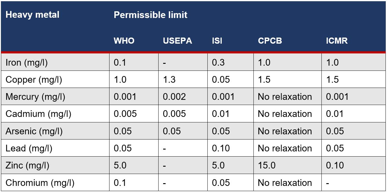
Scientific Research Question
To what extent can the detoxifying and filtrating properties of Typha Orientalis influence the contents of Copper (II) Sulfate and Cooking Oil in 10L of water.
Hypothesis
It is Hypothesised that the filtrating and detoxifying properties of Typha Orientalis reduces the amount Copper (II) Sulfate and Cooking oil in water. Supported by the research conducted by Kathe Seidel, the Typha Orientalis’ absorption of the mixture through its roots will result in a reduction in Cooking Oil and Copper (II) Sulfate (Sahtouris, E, 1990).
Table 1: Permissible limits of heavy metals in drinking water [63]
The Journal of Science Extension Research – Vol. 2, 2023 education.nsw.edu.au 176
Methodology
Materials
• 10x test tubes
• Test tube rack
• Copper testing kit
• Ruler
• 41.6 g of cooking oil
• 23.8 g of Copper (II) Sulfate
• 5L of Horticultural sand
• Latex gloves
• Face mask
• Scientific goggles
• 20L of water
• 2 air pumps
• Extension cord
• 8 bulrushes
• 2 buckets
• Small scales (g)
• Large scales (g)
• Petri dish
• Lab spatula and spoon
• 5L measuring cylinder
• 2 x 400mL beaker
• 100mL measuring cylinder
• 10mL measuring cylinder
All measuring equipment used was selected in proportion to the sample size needed to gain enough qualitative information for analysis.
Preparations
The room that was allocated by Peter Reeve and Brett McKay, was within a scientific lab, disturbed by students throughout the day.
Each bucket was placed on the large (kg) scales (tared) to measure 10kg of tap water (10L). Once equipped with face mask, scientific goggles and latex gloves, as per risk prevention methods [Appendix A, B], equal parts (2.5L or 2.5kg) of the horticultural sand was poured into each bucket, to simulate the environment and conditions needed for the bulrushes to grow. Then the bulrushes roots were buried into the sediment and the buckets were placed the same distance from the glass to ensure neither sample is receiving more/less light than the other.
The Air Pump, placed far enough away from any water, as per risk prevention methods [Appendix table C], was turned on and the air tight tube with the filter was inserted into each bucket.
With a face mask, latex gloves and scientific goggles, as per risk prevention methods [Appendix D,E,F], the small scales (g) and a petri dish (tared), were used to measure 23.8g (to 1 d.p) of Copper (II) Sulfate was measured onto the petri dish using the lab spoon and spatula, then poured into the bucket labelled ‘Copper (II) Sulfate’.
Using the small scales (g) and a 100mL beaker (tared), 41.6 grams of Cooking Oil (to 1 d.p) was measured, then poured into the bucket labelled ‘Oil’.
Method
From the materials extract 10x 10ml of the Copper (II) Sulfate sample and 10x 100mL of the Oil sample. Specifically for the Oil samples, take the measurements straight from the sample, i.e. don’t pour into beaker then measuring cylinder, as the Cooking Oil sits on top of the water and pouring out of the beaker continuously would result in some samples containing significantly more
The Journal of Science Extension Research – Vol. 2, 2023 education.nsw.edu.au 177
than others reducing the reliability. For the 10 Oil samples, leave for 30 minutes to settle as much as possible, then measure and record the level of Cooking Oil above the water (mL)
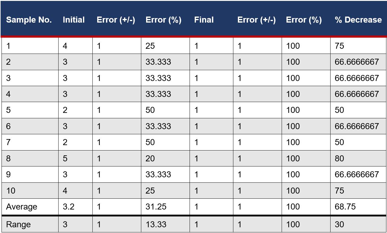

For the 10 Copper (II) Sulfate samples, the copper testing strips were inserted and left to process until dry. Then compared to the chart provided. Further quantitative data was measured using the scanner in the ‘What Colour Is this’ app, made by Nicholas Troia, to find the RGB scale. From this, the ‘B’ value of the copper test strips was recorded.
The same experimental process was repeated at the end of the 43 days to provide quantitative data to compare the change.
Results
Copper (II)
Content (ppm)
Sulfate
Table 1: Copper (II) Sulfate Content in ppm
The Journal of Science Extension Research – Vol. 2, 2023 education.nsw.edu.au 178
Table 2: Data gathered from Oil samples
Descriptive Statistics
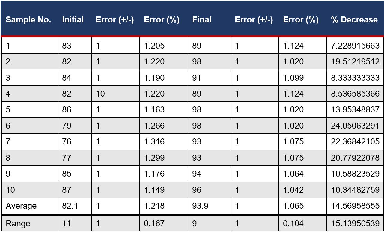
Alternate Hypothesis HA
It is Hypothesised that the filtrating and detoxifying properties of Typha Orientalis reduces the amount Copper (II) Sulfate and Cooking Oil in water.
Null Hypothesis H0
It is Hypothesised that the filtrating and detoxifying properties of Typha Orientalis will have no change in the amount of Copper (II) Sulfate and Cooking Oil in water.
Copper (II) Sulfate
T-Test: Two-sample Assuming Equal Variances
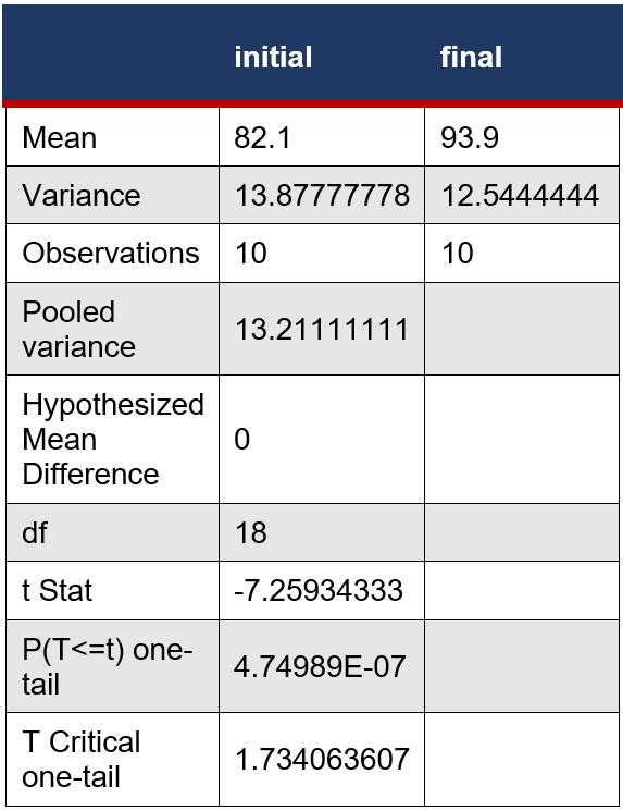 Table 3: Data gathered from Copper (II) Sulfate sample measured on the RGB scale
The Journal of Science Extension Research – Vol. 2, 2023 education.nsw.edu.au 179
Table 4: Descriptive statistics comparing the initial and final RGB scale of the copper test kit, measuring Copper (II) Sulfate
Cooking Oil
T-Test: Two-Sample Assuming Equal Variances
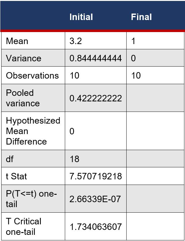
of mg, despite a difference in figures of ×103 the data still provided measurable differences, ultimately showing a greater change than predicted further justifying the use of Typha Orientalis in the filtration and detoxification of polluted bodies of water.
The Oil sample, over the course of 43 days in 10L of water, had reduced from an average of 3.2mL of Cooking Oil in 100mL samples to less than 1 ml in 100mL samples, a 68.75% decrease, measured through sedimentation. The initial samples ranged from 5mL to 2mL then finally decreased to scores of 1mL to <1mL but due to the limit of reading of 100mL measuring cylinders, +/- 1mL, the accuracy of the final assessment was reduced yielding an average percentage error of 31.25%. Alongside this due time constraints from study periods and time of breaks, the oil was only left to separate for 30 minutes reducing the accuracy of the data.
Discussion
The key research question was to explore the extent of Typha Orientalis’ filtration and detoxification properties within a realworld scenario, with materials based off of Sydney Harbour’s Water and The River Ganga samples, data gathered through scientific research conducted by Gavin Birch and the School of Geosciences at the University of Sydney (Birch, G., McCready, S., Long, E., Taylor, S., & Spyrakis, G., 2008) and Hasnahara Khatun and Dr. Arshad jamal (Khatun & Jamal, 2018). The average decrease in both tests demonstrated the success of the investigation, which was supported through descriptive statistics and qualitative data.
Due to a communication error, the substances were measured in g instead
Although the reduction in Cooking Oil after sedimentation was decreased significantly, as per the One-Tailed T-test, further testing with high precision equipment and minimal time constraints would provide a more accurate analysis.
Due to the law of conservation of mass, the outcome of the Cooking Oil sample would either be equal to or less than the initial amount of Cooking Oil, 41.6g, meaning a One-Tailed T-test was needed. The T-test was conducted (assuming equal variances) and according to the descriptive statistics table (table 4) TCrit= 7.570, PValue = 2.663E-07 and α = 0.05. As the PValue is <0.0001, there is >99.99% statistical significance in the difference in data sets, rejecting the null hypothesis and accept
Table 5: Descriptive statistics comparing the initial and final levels in mL of the Oil content
The Journal of Science Extension Research – Vol. 2, 2023 education.nsw.edu.au 180
the alternate hypothesis with strong statistical evidence.
The appearance of the sample initially, was clouded and large amounts of Cooking Oil were present above the water. It also left a thick layer of Cooking Oil on all of the equipment. The final appearance of the water was objectively much clearer with only a small film upon the surface of the water, different in colour to the original colour of the Cooking Oil, it acted in a different way to Cooking Oil, it took less time to complete sedimentation and was within 5 minutes as opposed to 30minutes to an hour

In the Cooking Oil sample, a small amount of frothy residue left upon the surface, meant it was in the emulsification stage of breaking up the oil, towards the end of the process, as outlined by (Ground truth Trekking, 2014). There was a mixture of white and brown foam (figure 2) which looked similar to seafoam that is present at the beach after a storm. This phenomenon was only present on the oil sample.

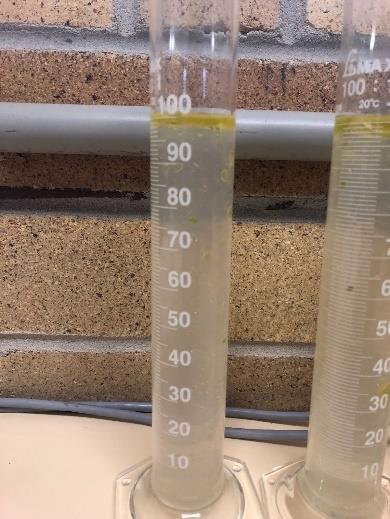 Figure 4: initial and final oil sample for comparison
The Journal of Science Extension Research – Vol. 2, 2023 education.nsw.edu.au 181
Figure 5: Frothy white/brown residue left on top of oil sample
The Copper (II) Sulfate sample, over the course of 43 days in 10L of water had decreased from an average of 2ppm to 1ppm, upon initial inspection of the copper test strip in a 10mL sample. Due to the large error associated with the Copper Testing Kit, each of the copper test strips were measured using a scanner in the ‘What Colour Is this’ app, made by Nicholas Troia, to find the RGB scale. From this, the amount of blue (B) was recorded, providing an increase from an average of 82.1B to 93.9B, a 14.57% increase in B, correlating to a 14.57% decrease in Copper (II) Sulfate. The initial samples (RGB) ranged from 76 to 87 then increased to range of 89 to 98. With a limit of reading of +/- 1B due to the App’s capabilities, the accuracy was decreased yielding an average error of 14.57%, which calls for more precise testing equipment. The use of the RGB scale provided a negative P-Value as there is an increase from the initial to the final results, but this is because an increase in the amount of ‘B’ correlates to the decrease in copper content in ppm, having no effect on the analysis.
Due to the law of conservation of mass, the outcome of the Copper (II) Sulfate sample would either yield the same amount of Copper (II) Sulfate or less, meaning a one-tailed t-test was needed. The t-test was conducted (assuming equal variances) and according to the descriptive statistics table (table 3) TCrit =7.259, PValue = 4.75E-07 and α = 0.05. As the Pvalue is <0.0001, there is >99.99% statistical significance in the difference in data sets, rejecting the null hypothesis and accept the alternate hypothesis with strong statistical evidence.
The Copper (II) Sulfate samples did not have a noticeable difference on camera,
but in person the final samples were much clearer than the initial samples with less blue from the Copper (II) Sulfate.
Note that due to the communication error stated above, the amount of Copper (II) Sulfate present would have been much greater than 2ppm, past the limit of reading of the copper test kit meaning it could not show a darker blue, but this was not discovered until a review of the investigation on 22/08/2022. Although it still decreased in Copper (II) Sulfate from 2382ppm down to approximately 1ppm. The same for the Cooking Oil, it would have decreased from 4164ppm down to approximately <1ppm.
The data gathered from each One-Tailed T-test, when measured comparatively, to show the efficiency of Typha Orientalis is similar in each data set. There was a 0.31137 difference between the TCrit, although the PValue of Copper (II) Sulfate is almost 2x more.
Table 5: Comparison of 2 Data Sets
As per WHO the final amount of copper found in the Copper (II) Sulfate sample was reduced from an unsafe amount of copper to the maximum acceptable amount of copper, 1ppm or 1mg/L (figure 3). The extension of this investigation, through extrapolation, would predict a decrease in copper and increase in water safety. This signified the success of the intention of the project, to detoxify and filtrate polluted water to a safe level.
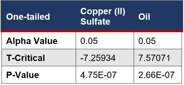
The Journal of Science Extension Research – Vol. 2, 2023 education.nsw.edu.au 182
Although there is no specific figure for the safe amount of PAH in drinking water, the assumption that as the number approaches 0 the safety reaches a maximum. Therefore, the reduction of oil, when extrapolated, would predict the regression of oil to a safe level in the future.
It is worth taking into consideration that this test was conducted throughout winter meaning the bulrushes were preparing to partially die off before producing new life in spring, leaving the potential for better results in spring/summer (Gardening With Angus Bringing You the Best In Australian Plants And Gardening, n.d.). Although, through studies conducted by Kathe Seidel, the dead or removed bulrushes would still provide sufficient filtration as long as the roots are alive (Sahtouris, E, 1990)
These findings can be applied to real world polluted water as the concentrations of Copper (II) Sulfate and Cooking oil were based on the data provided by (Birch, G., McCready, S., Long, E., Taylor, S., & Spyrakis, G., 2008) and (Khatun, H., & Jamal, D. A., 2018).
Conclusion
Typha Orientalis’ filtrating and detoxifying properties were proven to be effective in the reduction of Copper (II) Sulfate and Cooking Oil, as supported through quantitative and qualitative data. The Cooking Oil samples yielded an average decrease of 14.57% over the course of 43 days with a Pvalue that was <0.0001 (2.663E-07), there is >99.99% statistical significance in the difference in data sets, rejecting the null hypothesis and accept the alternate hypothesis with strong statistical evidence. The Copper (II)
Sulfate samples yielded an average decrease of 68.75% decrease over the course of 43 days. With a Pvalue <0.0001 (4.75E-07), there is >99.99% statistical significance in the difference in data sets, rejecting the null hypothesis and accept the alternate hypothesis with strong statistical evidence. The progressive visual clearing of both the Copper (II) Sulfate and Cooking Oil samples further reinforced the success of the investigation. The t-test and statistical analysis support the alternate hypothesis, rejecting the null hypothesis, further supporting the research conducted by Kathe Seidel (Sahtouris, E, 1990). These findings support the real-world application of this phenomenon.
Reference List
Adeel, M., Song, X., Wang, Y., Francis, D., & Yang, Y. (2017). Environmental impact of estrogens on human, animal and plant life: A critical review.
Environment International, 99, 107–119.
https://doi.org/10.1016/j.envint.2016.12.0 10
Australian Government, Fane, S., & Reardon, C. (2013). Wastewater reuse. Wastewater Reuse. Retrieved 16 October 2021, from https://www.yourhome.gov.au/water/wast ewater-reuse
Ben, Y., Hu, M., Zhang, X., Wu, S., Wong, M. H., Wang, M., Andrews, C. B., & Zheng, C. (2020). Efficient detection and assessment of human exposure to trace antibiotic residues in drinking water. Water Research, 175, 115699.
https://doi.org/10.1016/j.watres.2020.115 699
Birch, G., McCready, S., Long, E., Taylor, S., & Spyrakis, G. (2008). Contaminant
The Journal of Science Extension Research – Vol. 2, 2023 education.nsw.edu.au 183
chemistry and toxicity of sediments in Sydney Harbour, Australia: spatial extent and chemistry–toxicity relationships.
Marine Ecology Progress Series, 363, 71–88.
https://doi.org/10.3354/meps07445
Branley, A. (2015, July 7). Drugs including painkillers, anti-depressants found in tests on Sydney Harbour water. ABC News. Retrieved 10 November 2021, from https://www.abc.net.au/news/2015-0707/common-drugs-found-lurking-insydney-harbour-water/6599670
Brittanica. (n.d.). bulrush | plant Encyclopedia Britannica. Retrieved 2 November 2021, from https://www.britannica.com/plant/bulrush
Cassoobhoy, A. (2020). How does water pollution affect human health?.
Medicalnewstoday.com. Retrieved 13 February 2022, from https://www.medicalnewstoday.com/articl es/water-pollution-andhumanhealth#:~:text=Contaminated%20 water%20can%20harbor%20bacteria,hyg iene%2C%20or%20unsafe%20drinking% 20water
Chemical And Physical Information. (n.d.). GASOLINE. Retrieved 17 February 2022, from https://www.atsdr.cdc.gov/toxprofiles/tp72 -c3.pdf
Clinical Leadership and Infection Control. (2015, March 24). Chlorine used in wastewater treatment may boost antibiotic resistance, study finds. Retrieved 10 November 2021, from https://www.beckershospitalreview.com/q uality/chlorine-used-in-wastewatertreatment-may-boost-antibioticresistance-study-
finds.html#:%7E:text=Chlorine%20used% 20in%20wastewater%20treatment%20ma y%20boost%20antibiotic%20resistance% 2C%20study%20finds,-
Staff%20%2D%20Tuesday%2C%20Marc h&text=Recent%20research%20has%20 shown%20that,waste%2C%20contributin g%20to%20antibiotic%20resistance
Department of Primary Industries. (2020). NSW WeedWise. NSW WeedWise. Retrieved 8 June 2022, from https://weeds.dpi.nsw.gov.au/Weeds/Eur asianWaterMilfoil#:%7E:text=Eurasian%2 0water%20milfoil%3A,lakes%2C%20pon ds%20and%20shallow%20reservoirs%20 untitled%20(fluvalaquatics.com)
Doblin, M. (2014, August 29). A scientific understanding of Sydney Harbour University of Technology Sydney. Retrieved 23 November 2021, from https://www.uts.edu.au/research-andteaching/our-research/climate-changecluster/news/scientific-understandingsydney-harbour
Do, W., & Jamerson, M. (2021). Marine pollution. Wwf.org.au. Retrieved 13 February 2022, from https://www.wwf.org.au/what-wedo/oceans/marine-pollution#gs.phz2bc.
Engels, J. (2020, May 11). Collecting Clean Water from Polluted Sources with Natural Filtration Systems. The Permaculture Research Institute. Retrieved 17 June 2022, from https://www.permaculturenews.org/2020/ 05/15/collecting-clean-water-frompolluted-sources-with-natural-filtrationsystems/
Fell Consulting PTY LTD. (2015, May 30). WATER TREATMENT AND SYDNEY CATCHMENT. Discussion Paper for Office of NSW Chief Scientist and
The Journal of Science Extension Research – Vol. 2, 2023 education.nsw.edu.au 184
Engineer. Retrieved 10 November 2021, from
https://www.chiefscientist.nsw.gov.au/__d ata/assets/pdf_file/0020/63335/Finalwater-treatment-report-300514.pdf
FLUVAL. (n.d.). Air Pump Instruction Manual. Fluval Aquatics. Retrieved 14 June 2022, from https://www.fluvalaquatics.com/manuals/ Fluval_A849-A850-A82_QPump_Manual.pdf
Fuji Clean - USA. (2019, May 7). Fuji Clean USA - Wastewater Treatment Product Overview. YouTube. Retrieved 16 October 2021, from https://www.youtube.com/watch?v=LKJA QzeqE_M
FujiClean. (2008). Frequently Asked Questions | FujiClean. FujiClean Wastewater Treatment Systems. Retrieved 16 October 2021, from http://www.fujiclean.com.au/frequentlyasked-questions/
Gardening With Angus Bringing You the Best In Australian Plants And Gardening (n.d.). Gardening With Angus. Retrieved 30 November 2021, from https://www.gardeningwithangus.com.au/t ypha-orientalis-bullrush/
Government of South Australia. (n.d.). Department for Environment and WaterThe Department for Environment. . .. Department for Environment and Water. Retrieved 9 November 2021, from https://www.environment.sa.gov.au/topics /river-murray-new/improving-riverhealth/issues-for-river-health
Ground truth Trekking. (2014, November 5). Oil Degradation in the Sea. Retrieved 11 August 2022, from http://www.groundtruthtrekking.org/Issues
/AlaskaOilandGas/OilDegradation.html#: %7E:text=Biodegradation%20of%20oil% 20by%20microorganisms%20present%20 in%20the,the%20process%20of%20meta bolizing%20it%20to%20generate%20ene rgy
Illinois Department of Public Health. (n.d.). Polycyclic Aromatic Hydrocarbons (PAHs). Cancer in Illinois. Retrieved 10 November 2021, from http://www.idph.state.il.us/cancer/factshe ets/polycyclicaromatichydrocarbons.htm
Jenkins, J. (2019). The Humanure Handbook, 4th Edition: Shit in a Nutshell (4th ed.). Joseph Jenkins, Inc.
Khatun, H., & Jamal, D. A. (2018). Geochemicals Heavy Metal Pollution of River Ganga - Causes and Impacts. International Journal of Trend in Scientific Research and Development, Volume2(Issue-2), 1035–1038.
https://doi.org/10.31142/ijtsrd9576
LaRoche, C. (2019, March 2). Hazards of Copper Sulfate. Sciencing. Retrieved 14 June 2022, from https://sciencing.com/hazards-coppersulfate-7609349.html
Li, J., Yu, H., & Luan, Y. (2015). MetaAnalysis of the Copper, Zinc, and Cadmium Absorption Capacities of Aquatic Plants in Heavy Metal-Polluted Water. International Journal of Environmental Research and Public Health, 12(12), 14958–14973.
https://doi.org/10.3390/ijerph121214959
Millison, A. (2021, October 12). How to Recycle Waste Water Using Plants YouTube. Retrieved 24 October 2021, from https://www.youtube.com/watch?v=fsRcVkZ9yg&feature=youtu.be
The Journal of Science Extension Research – Vol. 2, 2023 education.nsw.edu.au 185
Mollison, B. (1997). Permaculture: A Designers’ Manual. Ten Speed Pr.
National Centre for Biotechnology Information. (n.d.). NCBI. NCBI. Retrieved 10 November 2021, from https://www.ncbi.nlm.nih.gov/pmc/articles/ PMC3945572/
National Herbarium of NSW, Royal Botanic Garden, Sydney, Australia. (n.d.). New South Wales Flora Online PlantNET. Retrieved 30 November 2021, from https://plantnet.rbgsyd.nsw.gov.au/cgibin/NSWfl.pl?page=nswfl&lvl=gn&name= Typha
NSW Department of Planning, Industry and Environment. (n.d.). Sydney Harbour - Beachwatch Daily Bulletins. Sydney Harbour Daily Pollution Forecast. Retrieved 23 November 2021, from https://www.environment.nsw.gov.au/bea chapp/SydneyBulletin.aspx?NoMobile
Oasis Design. (n.d.). Branched Drain Greywater Systems. Retrieved 24 October 2021, from https://oasisdesign.net/greywater/branche ddrain/
Office of Dietary Supplemets. (2021, March 29). Office of Dietary Supplements - Copper. National Institutes of Health. Retrieved 23 January 2022, from https://ods.od.nih.gov/factsheets/CopperHealthProfessional/
Perry, T. (2021, June 12). NASA says these 18 plants are the best at naturally filtering the air in your home. GOOD. Retrieved 23 November 2021, from https://www.good.is/slideshows/nasagets-
terrestrial?rebelltitem=18#rebelltitem18
Raine, R. (2020, November 17). Aquatic Plants That Purify Water. Home Guides | SF Gate. Retrieved 11 October 2021, from
https://homeguides.sfgate.com/aquaticplants-purify-water-43531.html
Rich, N. (2016, July 14). The Lawyer Who Became DuPont’s Worst Nightmare. The New York Times. Retrieved 16 October 2021, from https://www.nytimes.com/2016/01/10/mag azine/the-lawyer-who-became-dupontsworst-nightmare.html
Romano, M. (2019, January 19). Heavy Metal Test Kit. 5 in 1 Test Your Water For Harmful Metals. Retrieved 23 January 2022, from
https://www.alloratestkits.com.au/heavymetal-test-kits/
Sahtouris, E. (1990). Beautiful Bulrushes, Remarkable Reeds. Ratical. Retrieved 8 November 2021, from https://www.ratical.org/LifeWeb/Articles/ru shes.html
Sydney Institute of Marine Science Technical Report. (2014). Sydney Harbour A systematic review of the science 2014. Sydney Harbour Research Program. Retrieved 23 November 2021, from
https://www.sydneycoastalcouncils.com.a u/wp-content/uploads/2019/08/SydneyHarbour-A-systematic-review-of-thescience-2014.pdf
Sydney Water. (2021, July 6). Wastewater Treatment. Wastewater Treatment - Sydney Water. Retrieved 16 October 2021, from https://www.sydneywater.com.au/educati on/wastewater-recycling/wastewatertreatment.html
The Journal of Science Extension Research – Vol. 2, 2023 education.nsw.edu.au 186
The New York Times. (1975, March 9). Bulrushes Being Used in Artificial Marshes to Filter Water. Retrieved 2 November 2021, from https://www.nytimes.com/1975/03/09/arch ives/bulrushes-being-used-in-artificialmarshes-to-filter-water.html
UNSW. (2011, November 17). Sydney harbours deadly diet for sea creatures
UNSW Newsroom. Retrieved 23 January 2022, from https://newsroom.unsw.edu.au/news/scie nce-technology/sydney-harbours-deadlydiet-sea-creatures
UTS. (2020, October 20). Sewage to blame for beach contamination
University of Technology Sydney. Retrieved 10 November 2021, from https://www.uts.edu.au/news/healthscience/sewage-blame-beachcontamination
Victorian Government Department of Sustainability and Environment, & Murphy, A. H. (2006). National recovery plan for the Ridged Water-milfoil (Myriophyllum porcatum). Department of Climate Change, Energy, the Environment and Water. Retrieved 14 June 2022, from https://www.dcceew.gov.au/environment/ biodiversity/threatened/recoveryplans/national-recovery-plan-ridgedwater-milfoil-myriophyllum-porcatum
Water NSW. (n.d.). Our water supply system. WaterNSW. Retrieved 10 November 2021, from https://www.waternsw.com.au/waterquality/education/learn/water-supplysystem#:%7E:text=More%20than%2080 %25%20of%20Sydney’s,Blue%20Mounta ins%20and%20the%20Illawarra
Water Research Centre. (n.d.). pH of Drinking Water Natural Water and Beverages. Know Your H2O. Retrieved 16 November 2021, from https://www.knowyourh2o.com/indoor4/the-ph-of-
water#:%7E:text=The%20pH%20of%20p ure%20water,water%20and%20forms%2 0carbonic%20acid.
Wikipedia contributors. (2022, July 28). Warragamba River. Wikipedia. Retrieved 10 November 2021, from https://en.wikipedia.org/wiki/Warragamba _River
World Health Organisation. (n.d.). Copper. Retrieved 23 January 2022, from https://www.who.int/teams/environmentclimate-change-and-health/watersanitation-and-health/chemical-hazardsin-drinkingwater/copper#:%7E:text=Water%20Sanit ation%20and%20Health%20Our%20visio n%20and%20mission,document%20for% 20the%20development%20of%20the%20 GDWQ%20%282004%29
Writer, S. (2021, November 24). South Africa Faces Water Crisis Warns Rand Water. The Bulrushes. Retrieved 9 November 2021, from https://www.thebulrushes.com/2021/09/2 4/south-africa-faces-water-crisis-warnsrand-water/
YouTube. (2007, December 26). Ecomachine with Dr. John Todd Retrieved 8 November 2021, from https://www.youtube.com/watch?v=2jRek ZJx_-Q
Appendices
The Journal of Science Extension Research – Vol. 2, 2023 education.nsw.edu.au 187
Appendix
Appendix
Appendix
Appendix
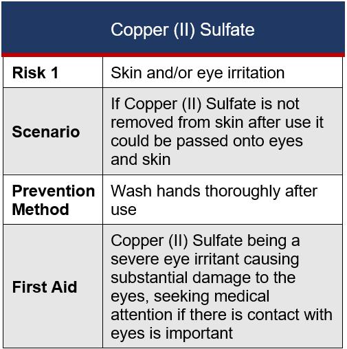
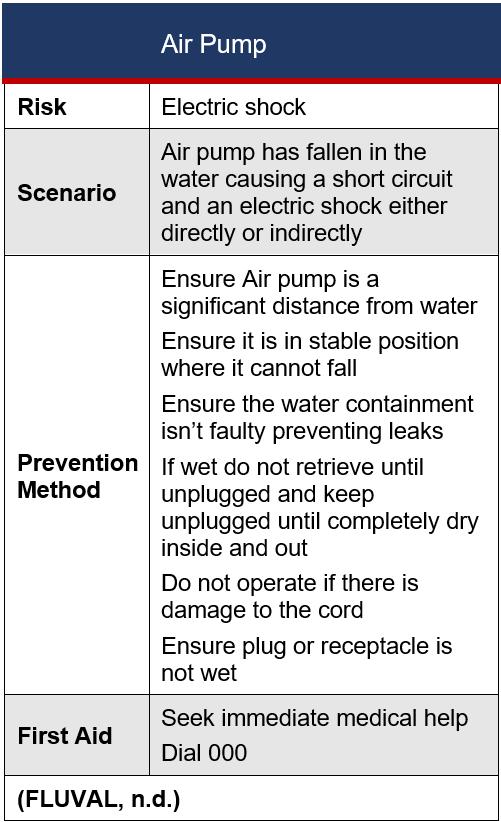
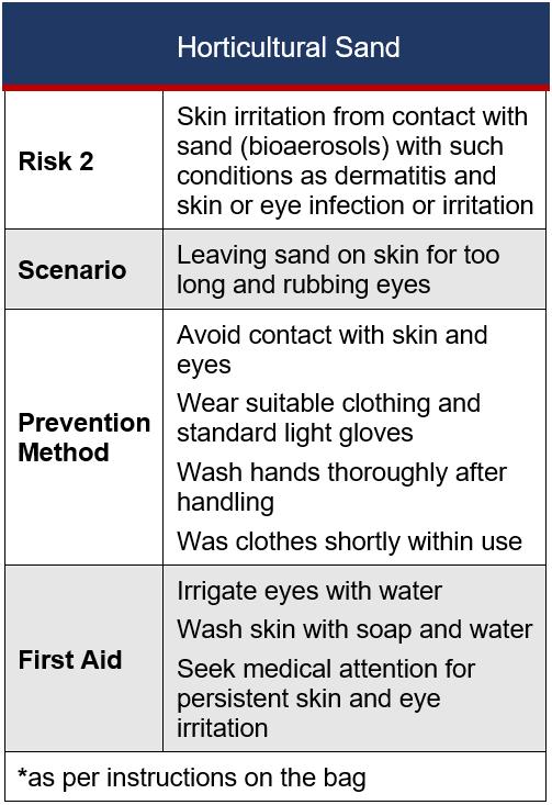
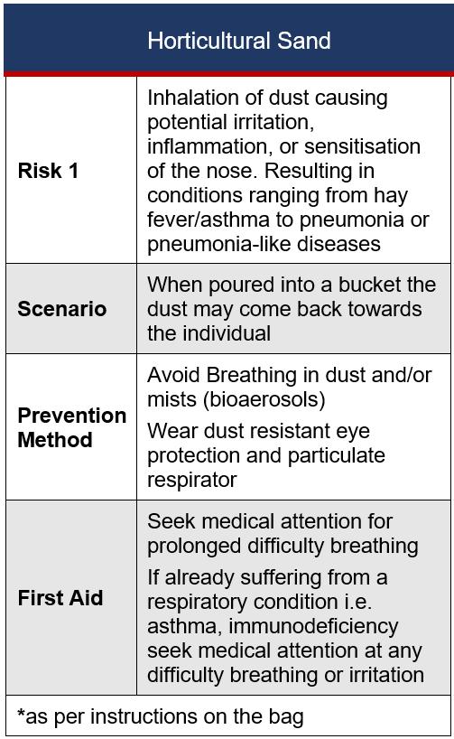 A: Risk Assessment 1 for Horticultural Sand
B: Risk Assessment 2 for Horticultural Sand
C: Risk Assessment for FLUVAL Air Pump
A: Risk Assessment 1 for Horticultural Sand
B: Risk Assessment 2 for Horticultural Sand
C: Risk Assessment for FLUVAL Air Pump
The Journal of Science Extension Research – Vol. 2, 2023 education.nsw.edu.au 188
D: Risk Assessment 1 for Copper (II) Sulfate
Appendix E: Risk Assessment 2 for Copper (II) Sulfate
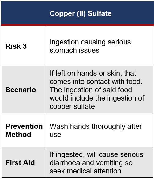
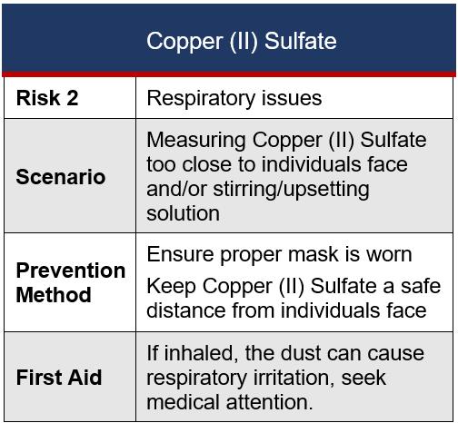
(LaRoche, C 2019)
Appendix F: Risk Assessment 3 for Copper (II) Sulfate
The Journal of Science Extension Research – Vol. 2, 2023 education.nsw.edu.au 189
Meta-study of the ability of seaweed farms to locally mitigate ocean acidification
Leroy Van Schellebeck
Coffs Harbour Senior College
This meta-study tested whether seaweed farms had the ability to locally mitigate ocean acidification using data taken from the report “Seaweed farms provide refugia from ocean acidification”. The report collected data on pH, Ωarag, O2 and CO2 levels in three seaweed farms and control sites outside of the seaweed farms. Out of these variables pH was selected as the best indicator of ocean acidification. It was hypothesised that in all three farms the mean pH will be higher with a significant difference to the control farms. An appropriate statistical test had to be selected to test for a significant different between the mean pH of the seaweed farms and control sites. The statistical test selected was a twosample t-test assuming equal variances with one tail using an alpha value of 5%. All three sites had a P-value lower than 2.225E-308. Similarly, the mean, maximum and minimum pH of the seaweed farms was higher than the control sites, except for Fodu Bays seaweed farms minimum pH, which was 0.01 lower than its control sites minimum pH. The hypothesis that the pH of the seaweed farms should be higher than the control sites was also supported by the mean, maximum and minimum pH levels for each. This resulted in the rejection of the null hypothesis that the pH of the seaweed farms would be lower or equal to the control sites.
Literature review
Ocean acidification
Ocean acidification is the continued decrease of the ocean’s pH due to the sustained increase in atmospheric carbon dioxide, which is absorbed by the oceans
��������2(����) ⇌��������2(��������) (Caldeira & Wickett, 2003). This dissolved carbon dioxide then reacts with water to form carbonic acid
��������2(��������) + ����2����(����) ⇌����2 ��������3(��������) then dissociating to produce hydrogen ions and bicarbonate ions ����2 ��������3 ⇌���� + + �������� ����3 . The increased concentration of hydrogen ions causes a change in pH (Gattuso and Hansson, 2011). This increase in free hydrogen ions shifts the equilibrium of the ocean’s carbonate and
hydrogen ions to form more bicarbonate ions �������� ���� + 3 ⇌���� + ��������2− 3 , resulting in fewer carbonate ions for calcifying organisms to form biogenic calcium carbonate ‘skeletons’, which become susceptible to dissolution (Orr et al., 2005).
Seaweed’s role in pH levels
Macroalgae’s can use photosynthesis, a redox reaction used by photoautotrophs to convert water and carbon dioxide into Trioses (three-carbon sugars) and oxygen using radiant energy from the sun as described by 3��������2�������� +6����2 ����(����) ⟶ ����3 ����6 ����3�������� +6����2 ����(���� ) (Raven et al., 2005; Reece et al., 2012). The decrease in dissolved carbon dioxide shifts the equilibrium, forming less carbonic acid
The Journal of Science Extension Research – Vol. 2, 2023 education.nsw.edu.au 190
and more water and dissolved carbon dioxide ����2 ��������3(��������) ⇌��������2(��������) + ����2 ����(����) . The drop in carbonic acid then changes the equilibrium of the dissociation of bicarbonate to form less hydrogen ions and bicarbonate “����2 ��������3 ⇌���� + + �������� ����3 ”. The decline in the concentration of hydrogen ions then increases the pH.
Evidence of macroalgae’s increasing pH
The effect communities of macroalgae’s and other macrophytes like seagrass have on local pH has been described as a way to protect small areas from deceased pH levels (Gattuso et al., 2018; Mongin, Baird, Hadley, & Lenton, 2016). The use of a seaweed farm near the Heron Island reef could buffer the projected rate of ocean acidification, protecting the majority of the reef for 7-21 years (Mongin, Baird, Hadley, & Lenton, 2016). Natural macroalgae and macrophyte communities in slow flow areas such as wave-sheltered bays or the canopies of seaweed/seagrass beds, are expected to give calcifiers a refugia from ocean acidification (Gattuso et al., 2018).
Conclusion
Ocean acidification has a range of negative effects on marine ecosystems, primarily effecting calcifying organisms (Kroeker et al., 2011). Photosynthetic organisms such as seaweeds increase pH as a by-product of photosynthesis which removes dissolved carbon dioxide from the water. Communities of macrophytes such as seaweeds can locally counter the effects of ocean acidification (Gattuso et al., 2018). Seaweed farms can then be used to mitigate ocean acidification and protect marine habitats (Mongin, Baird, Hadley, & Lenton, 2016).
Scientific research question
Are seaweed farms able to locally mitigate the effects of ocean acidification?
Scientific hypothesis
Hypothesis: The three farms studied will have a mean pH higher than the control site with a significant difference at an alpha value of 5%.
H1: μFarm
Null Hypothesis: The three farms studied will not have a mean pH higher than the control site with no significant difference at an alpha value of 5%.
Methodology
Using google scholar a suitable report to conduct a meta study on was searched for. The report “Seaweed farms provide refugia from ocean acidification” was a relevant, reliable credible and valid report. The report aimed to determine if seaweed farms provided refugia from ocean acidification. They used three different seaweed farms with control sites located at Nan’ao bay, Lidao Island and Fodu Bay (Fig. 1). Sensors were used to record data and water samples were taken at both the seaweed farms and the control sites outside of the farms. The report was chosen because it provided a range of data for the following dependent variables related to ocean acidification: pH, Ωarag, O2 and CO2. The report also recorded the position of the farm to the current and current direction, average current speed (cm s 1), tide type in the region, with maximum tide range, average tidal range, average flood & ebb tide duration, seawater quality (class (Inorganic
> μControl, α=0.05
≤
∴ P
0.05
����0 : �������������������� ≤ �������������������������������� , α=0.05 ∴ P>0.05
The Journal of Science Extension Research – Vol. 2, 2023 education.nsw.edu.au 191
Nitrogen (mg L 1) and Orthophosphate (mg L 1), dates of on-site monitoring and dates of the harvest season, salinity range (‰) and sea surface temperature range (°C). Measurements for positions of monitoring sensors and steps taken to calibrate and deploy, distance from control site and method for the titration of the water samples were also included. As
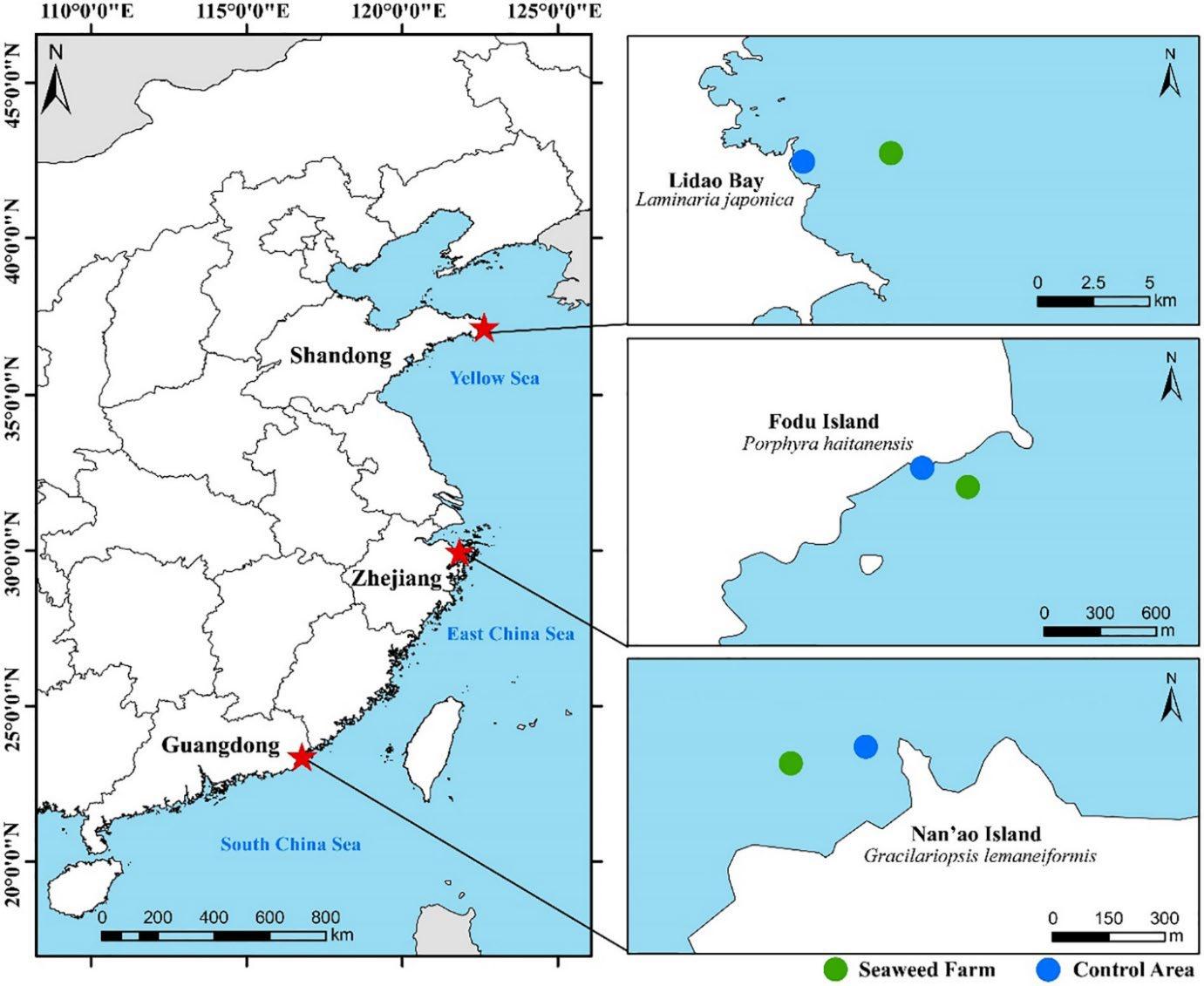
the report effectively accessed all relevant variables that they could not control and collected a wide range of relevant data it was selected to be used for the meta study. The reports recent publication date of 2021 and the authors high credibility furthered the report appeal to be selected for the meta study.
To keep the report simple and only test one relationship in the hypothesis only one dependent variable could be used. The best indicator of ocean acidification is pH level, so only the difference between the pH of the seaweed farm and control site was tested.
As the data used was normally distributed with a need to test for a significant difference; a t-test or ANOVA test could be used. As only two data sets where being tested for a difference, a t-test was
chosen. Some of the data from the control site or seaweed farm had brief gaps for all sites, so a paired sample for two means t-test could not be used as it relied on the count for both sets being equal. The variance for the seaweed farm and control sites pH was calculated to determine whether a two-sample t-test assuming equal variance or unequal variance should be applied. For each site the variance of the seaweed farm was divided by the variance of the control site to give a variance ratio. As the variance
Figure 1. A map of the location of the three sites data is sourced from report ‘Seaweed farms provide refugia from ocean acidification’ (Xiao et al., 2021).
The Journal of Science Extension Research – Vol. 2, 2023 education.nsw.edu.au 192
ratio for each site was less than four a two-sample t-test assuming equal variance was chosen as the appropriate ttest. As we were testing if the seaweed farm’s pH was not only significantly different to the control sites pH but also higher the directional one tailed t-test was selected. This meant the statistical test applied to each site was the two-sample t-test assuming equal variances with one tail. The standard alpha value of 5% or α=0.05 was used.
Results Nan’ao Island
The seaweed farm at Nan’ao Island had a mean pH of 8.15, 0.03 higher than the control sites 8.12 (Fig. 8). The seaweed farms minimum pH of 8.04 was 0.02 higher than the control sites 8.02 (Fig. 8). The maximum pH of 8.31 for the seaweed farm was 0.1 higher than the control sites 8.21 (Fig. 8).
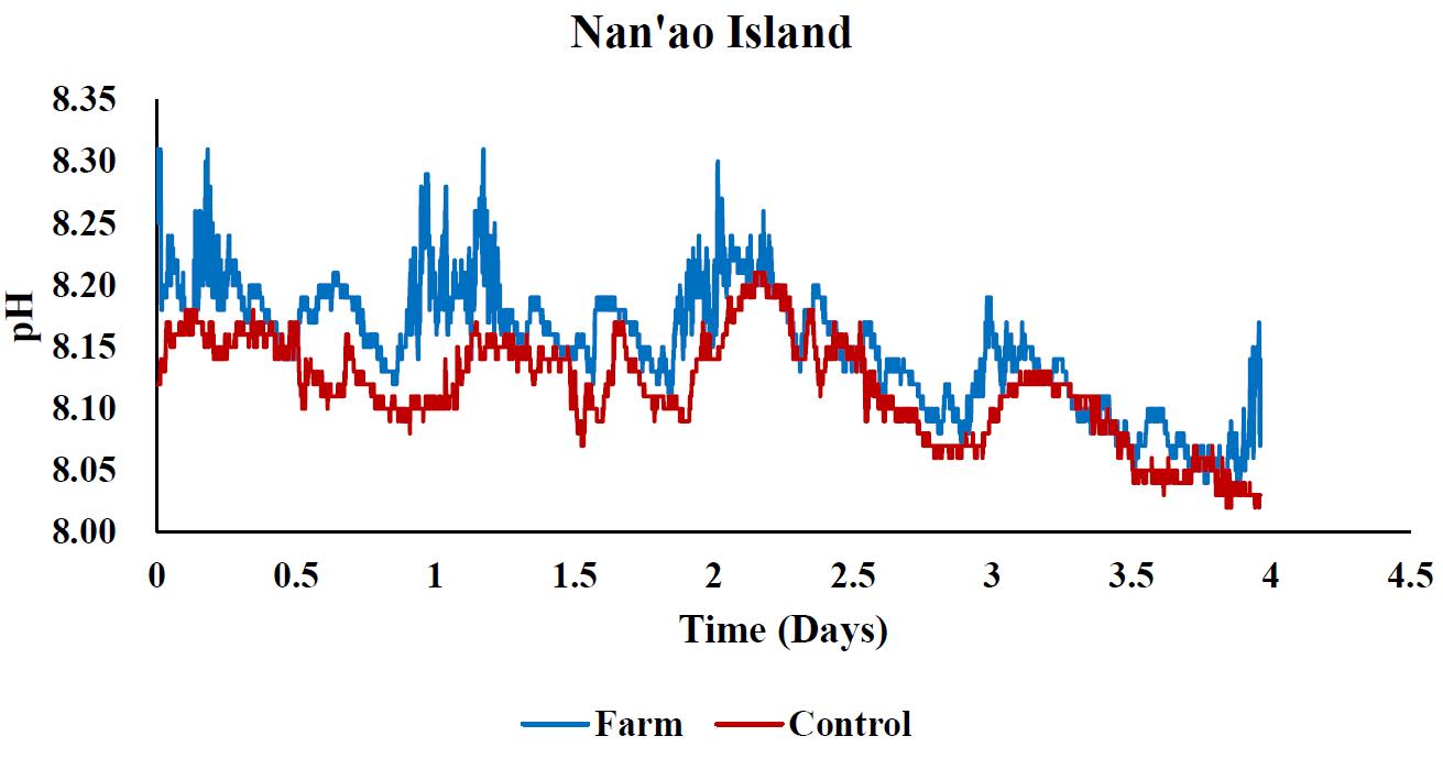
The two-sample t-test assuming equal variances with one tail gave a P-value of less than 2.225E-308, which was lower than the alpha value of 0.05 (Fig. 8). Equal variance is assumed as the variance ratio between the seaweed farm and control site is 1.5, less than the variance ratio of 4 needed for unequal variance to be assumed (Appendix 1).
The seaweed farm has a consistently higher pH with a significant difference between the control site (Fig. 2 and 3).
Figure 2. Line graph of the pH of the seaweed farm and control site at Nan’ao Island over four days from 11:00am on the 10th of May 2017 to 10:50am on the 15th of May 2017. I created the graph in excel using data is sourced from report ‘Seaweed farms provide refugia from ocean acidification’ (Xiao et al., 2021), see appendix for full data set.
Figure 3. Line graph of the moving average every 25 minutes of the pH of the seaweed farm and control site at Nan’ao Island over four days from 11:00am on the 10th of May 2017 to 10:50am on the 15th of May 2017. I created the graph in excel using data is sourced from report ‘Seaweed farms provide refugia from ocean acidification’ (Xiao et al., 2021), see appendix for full data set.
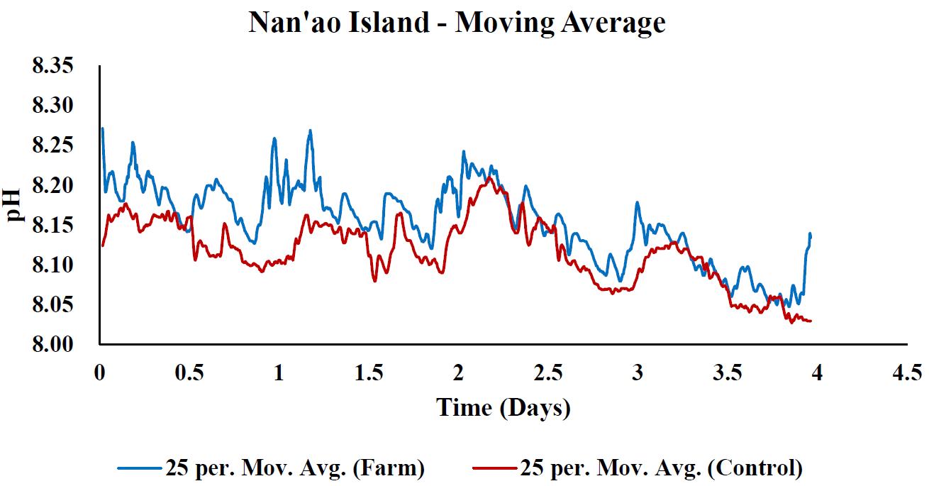
Lidao Bay
The seaweed farm at Lidao Bay had a mean pH of 8.12, 0.1 higher than the control sites 8.02 (Fig. 8). The seaweed farms minimum pH of 8.00 was 0.09 higher than the control sites 7.91 (Fig. 8). The maximum pH of 8.18 for the seaweed farm was 0.06 higher than the control sites 8.12 (Fig. 8).
The two-sample t-test assuming equal variances with one tail gave a P-value of less than 2.225E-308, which was lower than the alpha value of 0.05 (Fig. 8). Equal variance is assumed as the variance ratio between the seaweed farm and control site is 3.9, less than the variance ratio of 4 needed for unequal variance to be assumed (Appendix 2).
The Journal of Science Extension Research – Vol. 2, 2023 education.nsw.edu.au 193
The seaweed farm has a consistently higher pH with a significant difference between the control site (Fig. 4 and 5).
seaweed farm was 0.03 higher than the control sites 8.08 (Fig. 8).
The two-sample t-test assuming equal variances with one tail gave a P-value of less than 2.225E-308, which was lower than the alpha value of 0.05 (Fig. 8). Equal variance is assumed as the variance ratio between the seaweed farm and control site is 3.2, less than the variance ratio of 4 needed for unequal variance to be assumed (Appendix 3).
Figure 4. Line graph of the pH of the seaweed farm and control site at Lidao Bay over nine days from 6:11am on the 3rd of June 2017 to 5:30pm on the 12th of June 2017. I created the graph in excel using data is sourced from report
‘Seaweed farms provide refugia from ocean acidification’ (Xiao et al., 2021), see appendix for full data set.
The seaweed farm has a consistently higher pH with a significant difference between the control site (Fig. 6 and 7).
Figure 5. Line graph of the moving average every 25 minutes of the pH of the seaweed farm and control site at Lidao Bay over nine days from 6:11am on the 3rd of June 2017 to 5:30pm on the 12th of June 2017. I created the graph in excel using data is sourced from report
‘Seaweed farms provide refugia from ocean acidification’ (Xiao et al., 2021), see appendix for full data set.
Fodu Island
The seaweed farm at Fodu Island had a mean pH of 8.05, 0.02 higher than the control sites 8.02 (Fig. 8). The seaweed farms minimum pH of 7.97 was 0.01 lower than the control sites 7.98 (Fig. 8). The maximum pH of 8.11 for the
Figure
over twelve days from 8:53am on the 15th of November 2017 to 7:35pm on the 27th of November 2017. I created the graph in excel using data is sourced from report ‘Seaweed farms provide refugia from ocean acidification’ (Xiao et al., 2021), see appendix for full data set.
15th of November 2017 to 7:35pm on the 27th of November 2017. I created the
6. Line graph of the pH of the seaweed farm and control site at Fodu Island
The Journal of Science Extension Research – Vol. 2, 2023 education.nsw.edu.au 194
Figure 7. Line graph of the moving average every 25 minutes of the pH of the seaweed farm and control site at Fodu Island over twelve days from 8:53am on the
graph in excel using data is sourced from report ‘Seaweed farms provide refugia from ocean acidification’ (Xiao et al., 2021), see appendix for full data set.
The two-sample t-test assuming equal variances with one tail which was applied to each site gave a P-value of less than <2.225E-308 (Fig. 8). This value was lower than the alpha value of 0.05. Equal variance is assumed as the variance ratio between each seaweed farm and control site was less than the variance ratio of 4 needed for unequal variance to be assumed (Appendix 1-3).
Each sites seaweed farms mean pH was higher than the control sites mean pH (Fig. 8). Nan’ao Islands seaweed farm had the highest mean pH of 8.15 but had the second smallest difference in mean pH between the seaweed farm and control site of only 0.03 (Fig. 8). Lidao Bays seaweed farm had the second
highest mean pH of 8.12 and the largest difference in pH of 0.10 (Fig. 8). Fodu Bay had the lowest mean pH of 8.05 and the smallest difference of only 0.02 (Fig. 8).
The Nan’ao Islands seaweed farms minimum pH was 8.04 only 0.02 higher than the control sites minimum pH of 8.02 (Fig. 8). The Lidao Islands seaweed farms had a much higher minimum pH than its control site at 8.00, 0.09 higher than the control sites minimum pH of 7.91 (Fig. 8). Fodu Bay had a minimum pH of 7.97, 0.01 lower than the control sites minimum pH of 7.98 (Fig. 8).
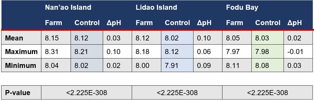
At each site the seaweed farms mean, maximum and minimum pH was higher than the control sites apart from Fodu Bays minimum pH, which was 0.01 lower than its control sites minimum pH ((Fig. 8).
Figure 8. A table of the mean, maximum and minimum pH for the seaweed farm and control sites as well as the difference in pH for each; along with the P-values from a two-sample ttest assuming equal variances with one tail for each site. Data is sourced from report ‘Seaweed farms provide refugia from ocean acidification’ (Xiao et al., 2021), see appendix for full data set.
Discussion
A future meta study on the same data could use different variables to access the relationship between seaweed farms and surrounding waters and test the other variable that are related to ocean
acidification like Ωarag and dissolved CO2. Different software should also be considered as excel did not have the precision to calculate numbers lower than 2.225E-308 resulting P-values of zero being presented. The high count of the data set made P-value very small, giving
The Journal of Science Extension Research – Vol. 2, 2023 education.nsw.edu.au 195
a very high significant difference. The graphs of each data set along with the means, maximums and minimums appear to support the hypothesis that the pH of the seaweed farm should be higher than the control site.
Despite the large amount of data collected by the original study monitoring only occurred for between four to twelve days varying for each site. Data was collected at different times of the year with different sized farms, along with a different species of seaweed being grown at each farm. This means it is hard to draw conclusions for what causes the difference in pH levels between the different seaweed farms. This variety on time, position, species, and sizes does mean that conclusions for the effects of seaweed farming in general are more valid as the conditions are more diverse across the three data sets. The validity makes for better general conclusions about how seaweed farms affect pH.
However, for the same reason any quantitative predictions for future studies on exactly how much a seaweed farm will affect pH cannot be extrapolated from this data. As a result, future studies would have to be completed to determine how best to use seaweed farms to locally ameliorate ocean acidification. These studies could extrapolate the rate of ocean acidification from predications of emissions scenarios based off other reports e.g., ‘Climate Change 2021: The Physical Science Basis’ (IPCC, 2021).
This provides a wide range for future studies that could access where and how seaweed farms would be most effective. Studies could simply determine the locations worst affected by ocean acidification, highlighting the areas in the
most need of seaweed farms. More indepth studies could also be undertaken to determine the best way a seaweed farm could reduce ocean acidification. This would involve modelling and testing the movement of water, different sizes of farms and species used to create optimum conditions to reduce ocean acidification. These studies could use multiple farms of the same species at different sizes or vice versa to achieve this. This could also be achieved using (name for tanks that ocean science experiments are run in) that would allow for a wide range of conditions to be tested, as well as future conditions such as lowered pH and warmer waters. This method would be able to effectively compare different species as all variables such as light, salinity water temp and water flow could be controlled.
Variation on the study accessed could also be undertaken. Measuring the effect on pH over the course of a year would help provide more concrete evidence for the positive long-term effects on local waters seaweed farms could have. Using multiple control sites for each farm at varying distances and positions relative to current and tidal flows would let the affects farms had on a larger area be accessed.
Conclusion
Each sites seaweeds farms mean, maximum and minimum pH was higher than the control sites, except for Fodu Bays minimum pH, which was 0.01 lower than its control sites minimum pH. The trends in (Fig. 2-7) displayed a generally higher pH of the seaweed farm over the control site. Each site had a P-value lower than 2.225E-308 due to limitations with excel more precise values could not
The Journal of Science Extension Research – Vol. 2, 2023 education.nsw.edu.au 196
be calculated. This gave all three farms a significant difference at an alpha value of 5% as the P-value was lower than 0.05 for all three. As the P-value was lower than the alpha value the null hypothesis was rejected as three farms studied did not have a mean pH lower than or equal to their control sites with no significant difference at an alpha value of 5%.
Reference list
Caldeira, K., & Wickett, M. E. (2003). Anthropogenic carbon and ocean ph. Nature, 425(6956), 365-365. doi:10.1038/425365a
Gattuso, J., & Hansson, L. (2011). Acidification: Background and history. Ocean Acidification.
doi:10.1093/oso/9780199591091.003.000 6
Gattuso, J., Magnan, A. K., Bopp, L., Cheung, W. W., Duarte, C. M., Hinkel, J., . . . Rau, G. H. (2018). Ocean solutions to address climate change and its effects on marine ecosystems. Frontiers in Marine Science, 5. doi:10.3389/fmars.2018.00337
Kroeker, K. J., Micheli, F., Gambi, M. C., & Martz, T. R. (2011). Divergent ecosystem responses within a benthic marine community to ocean acidification. Proceedings of the National Academy of Sciences, 108(35), 14515-14520. doi:10.1073/pnas.1107789108
Masson-Delmotte, V., P. Zhai, A. Pirani, S.L. Connors, C. Péan, S. Berger, N. Caud, Y. Chen, L. Goldfarb, M.I. Gomis, M. Huang, K. Leitzell, E. Lonnoy, J.B.R. Matthews, T.K. Maycock, T. Waterfield, O. Yelekçi, R. Yu, and B. Zhou. (2021). IPCC, 2021: Climate Change 2021: The Physical Science Basis. Contribution of
Working Group I to the Sixth Assessment Report of the Intergovernmental Panel on Climate Change. Cambridge University Press, Cambridge, United Kingdom and New York, NY, USA, In press, doi:10.1017/9781009157896.
Mongin, M., Baird, M. E., Hadley, S., & Lenton, A. (2016). Optimising reefscale co 2 removal by seaweed to buffer ocean acidification. Environmental Research Letters, 11(3), 034023. doi:10.1088/1748-9326/11/3/034023
Orr, J. C., Fabry, V. J., Aumont, O., Bopp, L., Doney, S. C., Feely, R. A., . . . Yool, A. (2005). Anthropogenic ocean acidification over the twenty-first century and its impact on calcifying organisms. Nature, 437(7059), 681-686. doi:10.1038/nature04095
Raven, PH, Evert, RF & Eichhorn, SE 2005, Biology of Plants, 6th edn, W.H. Freeman & Company, New York.
Reece, JB, Taylor, MR, Simon, EJ & Dickey, JL 2012, Campbell Biology: Concepts and Connections, 7th edn, Benjamin Cummings Publisher, San Francisco.
Xiao, X., Agustí, S., Yu, Y., Huang, Y., Chen, W., Hu, J., . . . Duarte, C. M. (2021). Seaweed farms provide refugia from ocean acidification. Science of The Total Environment, 776, 145192. doi:10.1016/j.scitotenv.2021.145192
The Journal of Science Extension Research – Vol. 2, 2023 education.nsw.edu.au 197
Characterisation of the Chaotic Behaviour of a Simple TwoTransistor Single-Supply Resistor-Capacitor Circuit
James Harrison Lambton High School
The claims of chaotic behaviour in the circuit proposed by Keuninckx et al. (2015) were investigated through utilising both in-situ and in-silico solutions. The circuit’s behaviour was characterised in two modes, depending on the location of the variable resistor, with the resistance range of chaotic behaviour observed within each mode varying between modes. Chaotic behaviour in both modes of the proposed circuit was found through the calculation of positive Lyapunov exponents across the range of resistances studied from simulation data. The validity of the simulation was confirmed as chaotic behaviour was observed for each mode in the in-situ circuit. Therefore, the claims of Keuninckx et al. (2015) were confirmed. The proposed chaotic circuit utilised cheap and readily available parts, hence, there is scope for its implementation in areas such as robotics or encryption, where chaos greatly increases efficiency and effectiveness.
Literature Review
Chaos theory is a mathematical theory which states that in dynamic systems displaying apparent randomness, there is underlying order within this apparent randomness. The theory involves the idea that chaotic systems are deterministic which means that, in principle, the future state of a system can be predicted mathematically (Oestreicher, 2007). However, this means that these systems are extremely sensitive to initial conditions, making it extremely difficult to predict the long-term state of these systems. The concept of chaos has been observed and articulated throughout human history, as evidenced by attributions to Aristotle, who observed that “the least initial deviation from the truth is multiplied later a thousandfold” (Aristotle, OTH). However, it was not until Edward Lorenz investigated chaotic behaviour in weather patterns when
interest in the study of chaotic systems exploded (Bishop, 2017). In 1961, Lorenz noticed that rounding to 3-digits during a meteorological calculation meant that the result greatly diverged from the results obtained when rounding to 6-digits (Oestreicher, 2007), discovering the idea of deterministic chaos. This laid the groundwork for chaos theory to exist, enabling the subsequent explosion of interest and research into the topic that has allowed for a deeper understanding of how chaos impacts human lives and how it can be used in real-world applications.
When describing chaotic systems, one thing to note is that a complex system does not imply a chaotic system and, likewise, a chaotic system is not always complex (Rickles et al., 2007). Complex systems involve many interactions between subunits whilst simple systems involve only a few interactions between subunits which behave according to
The Journal of Science Extension Research – Vol. 2, 2023 education.nsw.edu.au 198
simple laws. A chaotic system can be simple, with only a few subunits, which interact to create chaotic dynamics, with Sprott (1994), noting that chaos can surprisingly occur in very simple nonlinear equations. The study of chaos in simple systems is of particular significance, as it may have implications in many fields which deal in simple systems and yet experience chaotic behaviour. In the case of this investigation, the electronic circuit is an example of a simple system, as there are a limited number of well-defined components that make it function, however, it still will display chaotic behaviour because of the non-linear dynamics which govern it.
There is a need for flexible, low-cost chaotic systems based around electronic circuits because a variety of applications, such as robotics and encryption, are emerging which can utilise chaos in order to be more effective (Tanougast, 2011). An application which could utilise chaos theory is that of encryption. Chaotic encryption would be significantly harder to decrypt by brute force, and providing the idea of deterministic chaos holds true, would allow for the desired user to easily access the information if they have access to an encryption key outlining the initial conditions of the system. One area of encryption which could utilise chaos theory is image encryption, detailed by Shaukat et al. (2020). Chaotic properties of complex dynamics, deterministic behaviours, ergodicity, pseudorandomness, high sensitivity to initial conditions, etc. allow for the creation of a more secure encryption method. The use of these chaotic properties allows for a highly random sequence to be generated based on a chaotic system, instead of the classical algorithm, which allows for a
more secure and efficient image encryption method over conventional techniques. Shaukat et al. (2020) propose several recommendations for future research and development of image encryption utilising chaos theory; the most notable of these is the need for practical and feasible methods of generating chaotic dynamics, as many proposed methods have extensive hardware requirements due to computational complexities. This could be addressed through continued research and application of chaotic circuits constructed from simple and low-cost components, both in their physical form and simulated software form. Similarly, the use of chaotic circuits in robotics may also greatly improve the functionality of these systems. The current autonomous robotic solutions are limited in their behavioural patterns, however, through the use of a chaotic system, the potential number of behavioural patterns can be increased for these autonomous robots (Steingrube et al., 2011).
The first chaotic circuit proposed and created was by Leon Chua who mathematically determined and designed a circuit which displayed chaotic behaviour. Chua’s circuit (shown in Figure 1) was incredibly simple, consisting of an inductor (L), two capacitors (C1 and C2), a linear resistor (R) and a negative non-linear resistor (NR), and it is simply this non-linear resistor which makes the circuit chaotic, as the other four are linear elements (CHAOTIC CIRCUITS, 2015) This simple design has paved the way for the development of most chaotic circuits, either by adding elements to increase their chaotic behaviour or using similar mathematical ideas to put into circuital implementation. However, many of these
The Journal of Science Extension Research – Vol. 2, 2023 education.nsw.edu.au 199
circuits, including Chua’s circuit, utilise complex components (such as inductors, analogue multipliers, or operational multipliers) in order to display chaotic behaviour, which is not necessarily disadvantageous within itself, but avoiding such elements would be beneficial in terms of cost and circuit complexity. This would also simplify the ability to model such circuits through software simulation which would allow chaotic behaviours to be more easily integrated into applications. Furthermore, there is no correlation between the use of these complex components and the degree to which the circuit displays chaos, therefore, if an effective simple circuit using readily available parts was developed, this would be more desirable from a cost and logistics stand-point (Keuninckx et al., 2015).
(as it is less straightforward to integrate circuits containing elements such as inductors) and it is much more cost effective, as well as easier to construct, due to a low parts count (Keuninckx et al., 2014). The circuit is also described by four relatively simple differential equations (Figure 3), which means that the state of the system at a given point can be easily determined mathematically. Furthermore, neither the values for the components nor the supply voltage are critical, and the frequency range is scalable (Keuninckx et al., 2015); the implications of this circuit design are that it can be utilised and adapted into a variety of applications which could take advantage of chaos, such as image encryption or robotics.
Keuninckx et al. (2015) proposed a simple two-transistor single-supply resistor-capacitor chaotic oscillator where the circuit designed utilises a transistorbased RC-ladder with a small onetransistor subcircuit directly attached to this RC-ladder (represented by the dashed box in Figure 2), adding a new equilibrium to the system in which Q1 also is biased as an active amplifier, enabling chaotic oscillations and behaviour. Therefore, as there are no complex components, the advantage of this circuit lies in its simplicity because it is much easier to model mathematically
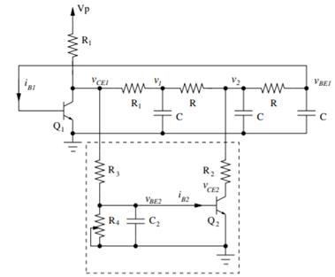
 Figure 1. Chua’s Circuit
The Journal of Science Extension Research – Vol. 2, 2023 education.nsw.edu.au 200
Figure 2. A simple two-transistor singlesupply resistor-capacitor circuit (Keuninckx et al., 2015).
Scientific Research Question
The investigation will model and experimentally confirm the chaotic behaviour in a simple two-transistor single-supply resistor-capacitor chaotic oscillator with the aim of confirming the claims by Keuninckx et al. (2015) that two circuit layouts, where the location of the variable resistor is switched between R3 and R4, of chaotic behaviour can be observed with this circuit design.
Scientific Hypotheses
H0: If the position of the variable resistor (R4) within the circuit is changed, then the circuit will not display chaotic behaviour in this new circuit layout across the range of resistances studied.
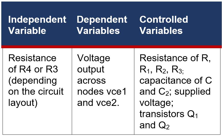
HA: If the claim by Keuninckx et al. (2015) is true, then when the position of the variable resistor R4 within the circuit is changed to the position of R3 (and R4 is replaced by the resistor R3), then the circuit will continue to display chaotic behaviour in this new circuit layout, evidenced by generating positive Lyapunov exponents, across the range of resistances studied.
Variables
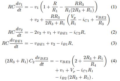
Methodology
Part 1: Circuit Design and Physical Construction
The physical circuit was constructed on a breadboard, shown in Figure 4, based on the circuit design of Keuninckx et al. (2015), shown in Figure 5. Off-the-shelf physical components for the circuit were sourced Core electronics and element14. The resistances of a few resistors were slightly changed as resistors with their exact resistances were not readily available. These differences in resistance were not very significant and are attributed to rounding and generalisation by Keuninckx et al. (2015). Figure 4 shows the completed circuit on the breadboard in Mode 1, the primary design reported by Keuninckx et al. (2015), where the variable resistor is located at R4 and a fixed resistor at R3. While Mode 2 has the variable at R3 and the fixed resistor located at R3.
Part 2: Software experimentation using LTSpice
In order to obtain data which can be analysed using TISEAN software (Hegger et al., 1999), the platform LTSpice was utilised. It is not feasible using the equipment and technology available for this research to collect specific data
Figure 3. Differential equations which describe the circuit in Figure 2 (Keuninckx et al., 2015).
The Journal of Science Extension Research – Vol. 2, 2023 education.nsw.edu.au 201
points in a physical model of the circuit across a 20ms timestamp, hence a LTSpice simulation of the circuit was used. Using LTSpice, the Mode 1 circuit proposed by Keuninckx et al. (2015) was created, shown in Figure 6, and simulations were run for varying resistances of R4. Voltage measurements were taken across the nodes vce1 and vce2 to monitor the chaotic behaviour of the circuit. These graphs can be compared to the output graph of the oscilloscope produced by the physical circuit in order to confirm the validity of the simulation. One output which should display chaos is the voltage across the node vce1, according to Keuninckx et al. (2015), therefore, voltage readings across this node was taken across a 20ms time period (as shown in the in-silico vce1 vs. time data given in in Figures 7 and 8). This data was generated for integer resistances of R4 between 35kΩ and 75kΩ to show the range of resistances where chaos is generated. This was then repeated for the circuit in Mode 2 (with integer resistance between 15kΩ and 70kΩ), with the resistance of R3 being changed and the resistance of R4 kept constant at 40kΩ. The data was then analysed using the TISEAN software to calculate Lyapunov values where chaotic voltages were observed.
30kΩ, C = 1nF, C2 = 360pF, and VP = 5V.

(Keuninckx et al., 2015)
Part 3: Conducting the practical experimentation
The goal of the practical experimentation using a physical circuit on a breadboard was to confirm the results obtained from the software simulation in order to demonstrate the validity of the data obtained from this simulation. An oscilloscope (QC1932 Digitech Digital Oscilloscope) was used to obtain the results of the physical circuit which produced a graph of voltage versus time across vce1 and vce2. Due to limitations of the oscilloscope, traces for the oscillations in voltage across the node vce1 could not be clearly seen so only oscilloscope traces for voltage across the node vce2 versus time were obtained.
Conducting data analysis using TISEAN
The TISEAN analysis package (Hegger et al., 1999) was used to analyse and quantify the non-linear behaviour
Figure 4. The circuit shown is physically made on a breadboard with R4 as the variable resistor (mode 1).
Figure 5. A simple two-transistor singlesupply resistor-capacitor circuit. The components have the following values: R = 10kΩ, R1 = 5kΩ, R2 = 15kΩ, R3 =
The Journal of Science Extension Research – Vol. 2, 2023 education.nsw.edu.au 202
observed in this study; the function of calculating the maximal Lyapunov exponent was used in order to demonstrate whether or not chaos occurs in the circuit at a variety of resistance in both modes of the circuit. The Cygwin platform was utilised to run the TISEAN analysis package. The ‘lyap_k’ function from the package was used to calculate the suite of Lyapunov exponents which uses the Kantz algorithm (Kantz, 1994).
Results
Physical Validation of Simulation:
A comparison of the in-situ experiment with a voltage probe on vce2 measuring voltage and the in-silico experiment with

voltage measured across vce2, shown in Figures 7 and 8, show that chaos is exhibited in both modes in the physical circuit. This chaos is shown by the erratic, inconsistent signal produced which draws similarities to that of the in-silico simulation. While the in-situ graph displays slight discrepancies of spikes in voltage, these are most likely caused by minor variations in component performances and limitations associated with the oscilloscope to measure the small voltage fluctuations observed. An adjustment of the variable resistor in each circuit showed chaos exhibited across a variety of resistances in both in-situ and in-silico circuits.
Visual Analysis of LTSpice Simulation:
Figure 7. Mode 1; right – in-situ oscilloscope display (voltage vs. time); left – in-silico voltage vs. time plot
Figure 8. Mode 2; right – in-situ oscilloscope display (voltage vs. time); left – in-silico voltage vs. time plot
The Journal of Science Extension Research – Vol. 2, 2023 education.nsw.edu.au 203
When voltage across nodes vce1 and vce2 (in Mode 1 and Mode 2) are plotted against each other the graph of the chaotic attractor shown in Figure 9 and 11 is produced, which shows bistable oscillations around two unstable equilibria, indicative of the chaotic behaviour of the circuit. Similarly, when voltage across nodes vce1 and v1 are plotted against each other in Figure 10 and 12, this same chaotic attractor of oscillations around two unstable equilibria can be seen.
Summary of Results:
Figures 13 and 14 show the range of voltage achieved by each circuit as well
as the range of resistances across which chaotic behaviour occurs within the circuit. The gaps in the area map indicate periodic behaviour within the circuit where chaotic behaviour was not observed.
Figure 9. vce1 vs. vce2, for R4 = 40kΩ Figure 10. vce1 vs. v1, for R4 = 40kΩ
Figure 11. vce1 vs. vce2, for R3 = 24kΩ Figure 12. vce1 vs. v1, for R3 = 24kΩ
The Journal of Science Extension Research – Vol. 2, 2023 education.nsw.edu.au 204
Statistical Analysis:
The statistical test carried out utilised the procedure for the testing of chaotic dynamics by Bask & Gençay (1998). The Lyapunov exponents used were
calculated using the TISEAN software (Hegger et al., 1999). The chaotic behaviour of the circuit in Mode 1 characterised by Lyapunov exponents in Table 1 show that there is a distinct range across which chaos occurs. The results
 Figure 13. Area map highlighting upper and lower voltage range at vce1 between which chaotic behaviour was detected as a function of resistance at R in Mode 1.
Figure 14. Area map highlighting upper and lower voltage range at vce1 between which chaotic behaviour was detected as a function of resistance at R in Mode 2.
Figure 13. Area map highlighting upper and lower voltage range at vce1 between which chaotic behaviour was detected as a function of resistance at R in Mode 1.
Figure 14. Area map highlighting upper and lower voltage range at vce1 between which chaotic behaviour was detected as a function of resistance at R in Mode 2.
The Journal of Science Extension Research – Vol. 2, 2023 education.nsw.edu.au 205
found that chaotic behaviour (i.e. the range across which positive Lyapunov exponents were calculated) occurs between 39kΩ and 70kΩ. Similarly, the chaotic behaviour of the circuit in Mode 2 characterised by Lyapunov exponents in Table 2 shows that there is a less distinct range across which chaos occurs. The results found that chaotic behaviour occurs between 17kΩ and 55kΩ, however, there were significantly more and longer periods of non-chaotic behaviour within this range compared to Mode 1. These ranges of resistance are
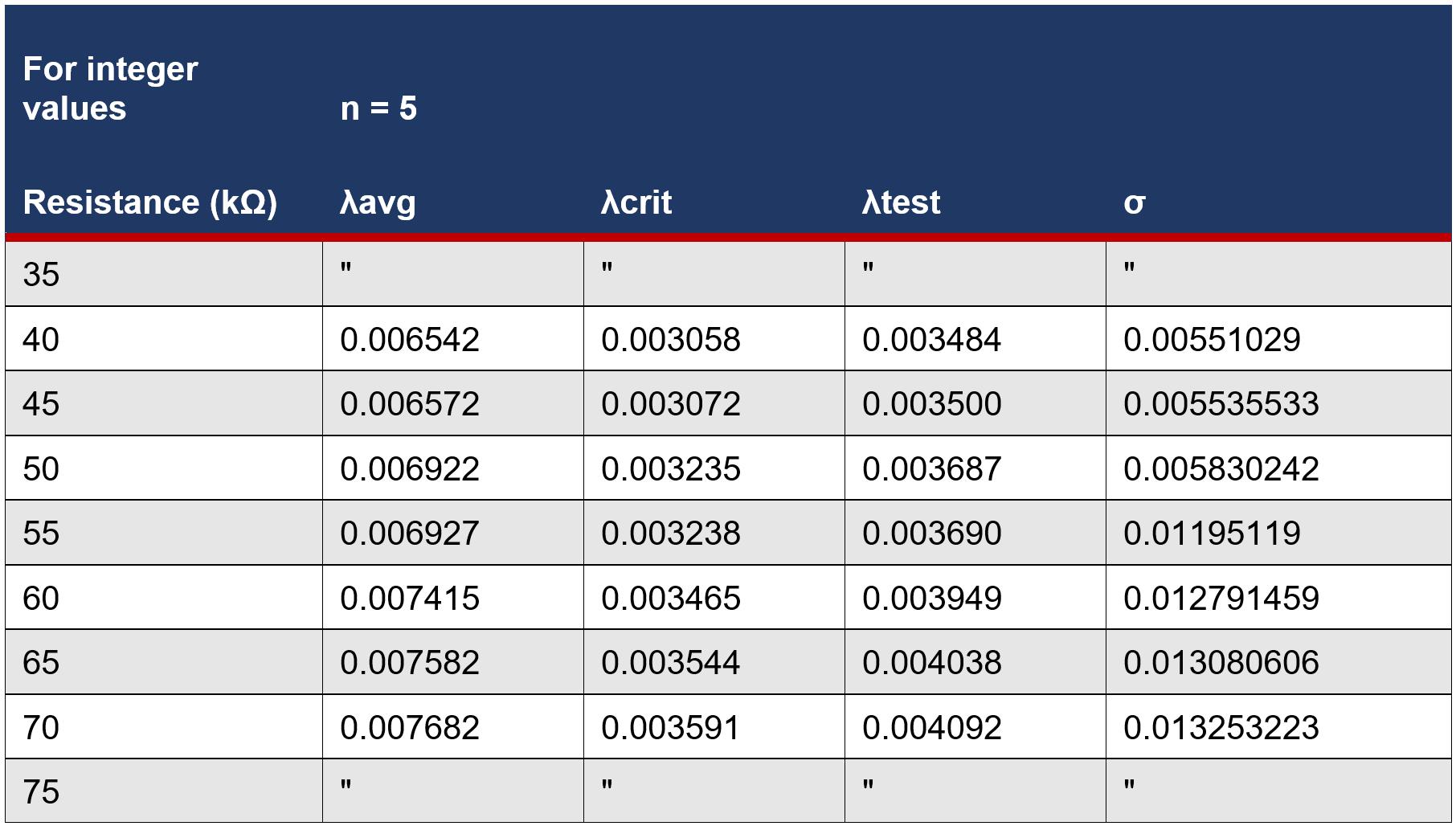
consistent with the graphs in Figure 11 and 12. All Lyapunov exponent values across all resistances in both modes were fairly small (with all λ < 1x10⁻¹), indicating that observed chaotic behaviour in the circuit is weak. The magnitude of the Lyapunov exponents increased with increasing resistance (and thus an increase in chaotic behaviour) in Mode 1, whereas the inverse is true in Mode 2 as the magnitude of Lyapunov exponents decrease with increasing resistance (a weakening in chaotic behaviour)
Mode 1
Table 2. Summary of hypothesis test for Mode 1 of the circuit. α = 0.025. H0: λtest ≤ 0 vs. HA: λtest > 0.
The Journal of Science Extension Research – Vol. 2, 2023 education.nsw.edu.au 206
Mode 2
Discussion
There exists a need for cheap and flexible simple chaotic circuits in fields such as robotics or encryption, (Tanougast, 2011), hence, this study has characterised the chaotic behaviour of the circuit proposed by Keuninckx et al. (2015) in two modes of the circuit. The findings of the study successfully demonstrate that chaotic behaviour occurs within both Mode 1 and Mode 2 of the circuit, both in-situ and insilico across a range of resistances, as positive Lyapunov exponents were obtained, therefore, the null hypothesis can be rejected, confirming the claims of chaotic behaviour by Keuninckx et al. (2015). The chaotic behaviour of the circuit was experimentally confirmed utilising an in-situ physical model of the circuit as expected oscillations in voltage, comparable to that of the LTSpice simulation of the circuit, were observed in both modes. Therefore, the further
analysis done on using the simulated circuit is valid as it has been experimentally confirmed that chaotic behaviour does exist within the circuit.
Positive Lyapunov exponents (λ) were obtained across a range of resistances in both circuit modes, which is a strong indication of chaotic behaviour. This chaotic behaviour occurs in the circuit due to the feedback to the input from the components in the dashed box in Figure 2 (CHAOTIC CIRCUITS, n.d.) which creates a phase shift, inducing chaotic oscillations across the circuit. Interestingly, the range of resistances across which chaotic behaviour occurred in both modes was different as Mode 1 exhibited chaos from resistances between 39kΩ and 70kΩ, while Mode 2 from 17kΩ and 55kΩ, and the chaotic behaviour of Mode 2 was much more erratic and discontinuous with more and longer interspersed periods of periodic behaviour (λ < 0). This may bring into
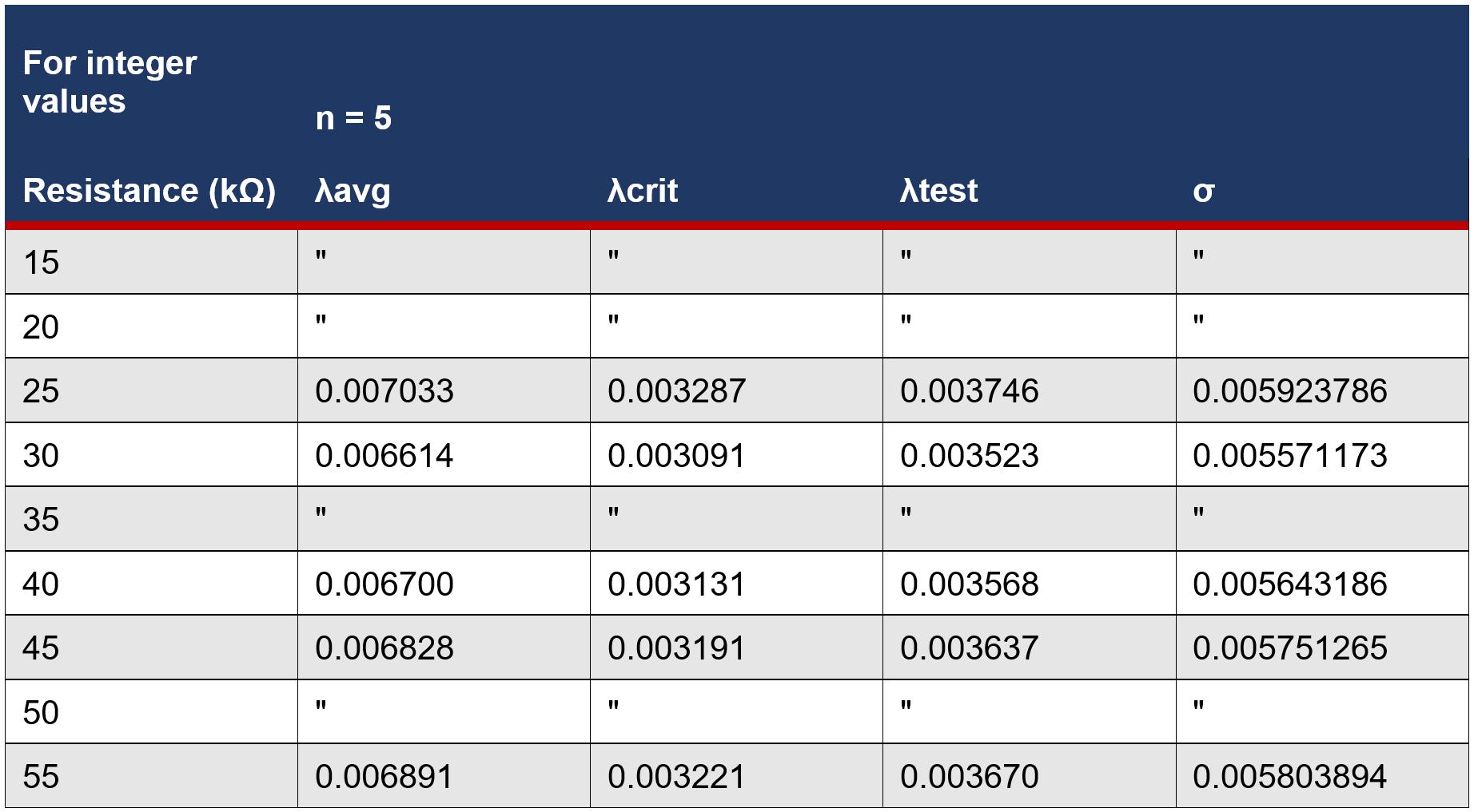 Table 3. Summary of hypothesis test for Mode 2 of the circuit. α = 0.025. H0: λtest ≤ 0 vs. HA: λtest > 0.
The Journal of Science Extension Research – Vol. 2, 2023 education.nsw.edu.au 207
question the effectiveness of using Mode 2 in applications where consistent chaotic behaviour is needed, however, this interspersion of periodic behaviour may suit some applications where a both periodic and chaotic behaviour is needed. The values for the magnitude of the components (and the exact model of the transistor) used in this study differed slightly from the proposed components by Keuninckx et al. (2015), however, chaotic behaviour was still observed, indicating that this circuit design can be flexibly applied for a range of purposes in terms of cost and availability of the components Therefore, the chaotic circuit design characterised in this study is flexible and cheap (through utilising off-the-shelf components), providing the groundwork for future development of arrangements of similar circuit designs. This also increases the potential utility of such circuit designs in a wide variety of applications.
These findings of chaotic behaviour in the circuit are consistent with the findings of Keuninckx et al. (2015), who reported chaotic behaviour within Mode 1 circuit used, along with CHAOTIC CIRCUITS (n.d.) who also reported chaotic behaviour in this same circuit design. Chaotic behaviour in a circuit utilising relatively simplistic components is also consistent with the mathematical modelling by J. C. Sprott (2000) who found that chaos occurred in similar circuits.
The implications of a low-cost, flexible circuit made from off-the-shelf components are that it can be readily applied into physical applications at lowcost such as in image encryption or in robotics as the utilisation of chaos theory will greatly optimise and increase the
efficiency of robotic functions and algorithms, especially when coupled with other technologies such as artificial intelligence or machine learning (Zang et al., 2016). This will allow for a new level of optimisation and productivity in these applications, such as in sensori-motor systems in complex robots (Steingrube et al., 2011), which could not be achieved with current, non-chaotic solutions. Moreover, the straightforward digital implementation of this circuit to create chaos could be useful not only for simulating certain patterns of chaos, but also for a range of software-based applications where chaos can be used to generate encryption keys or noise patterns.
Future research should be done into variations of this chaotic circuit design which utilise the resistor-capacitor feedback loop in order characterise a greater range of circuit designs using offthe-shelf components that display modes of chaotic behaviour. An improvement on the investigation could be through utilising greater quantifiers of chaos (such as fractals) as opposed to the simple maximal Lyapunov exponent calculation that was utilised using TISEAN software (Hegger et al., 1999). Hence, a possible direction for future research could be into quantifying the chaotic behaviour of this circuit (or circuits similar to it) across resistances on a micro-level utilising higher order chaotic quantifiers in order to observe the extent to which the circuit displays chaos.
The Journal of Science Extension Research – Vol. 2, 2023 education.nsw.edu.au 208
Conclusion
This study confirmed the claim by Keuninckx et al. (2015) of chaotic behaviour in the proposed circuit in Mode 2, as well as Mode 1, by demonstrating that chaos occurs in both in-situ and insilico solutions. Through the use of data from the simulated circuit, positive Lyapunov exponents were obtained, rejecting the null hypothesis and indicating the range of resistances where chaotic behaviour occurs within the circuit. The circuit proposed is flexible and cheap, therefore, future research should be directed towards applying this flexible circuit into applications where the implementation of chaos greatly improves their efficiency and effectiveness, such as robotics and encryption.
Acknowledgements
I would like to thank Mr. Nicholson for his valuable guidance and feedback across all stages of developing, conducting, and finalising the report.
Reference List
Aristotle (1985) [OTH], On the Heavens,; in. J. Barnes (ed.), The Complete Works of Aristotle: The Revised Oxford Translation, Vol 1. Princeton: Princeton University Press. (n.d.).
Bask, M., & Gençay, R. (1998). Testing chaotic dynamics via Lyapunov exponents. Physica D: Nonlinear Phenomena, 114(1), 1–2.
https://doi.org/10.1016/S01672789(97)00306-0
Bishop, R. (2017). Chaos. In E. N. Zalta (Ed.), The Stanford Encyclopedia of Philosophy (Spring 2017). Metaphysics Research Lab, Stanford University.
https://plato.stanford.edu/archives/spr201 7/entries/chaos/CHAOTIC CIRCUITS. (n.d.). CHAOTIC CIRCUITS. Retrieved 4 December 2021, from
https://www.chaotic-circuits.com/
Davies, B. (2018). Exploring Chaos: Theory And Experiment. CRC Press.
Guan, K. (n.d.). Important Notes on Lyapunov Exponents. 18.
Hegger, R., Kantz, H., & Schreiber, T. (1999). Practical implementation of nonlinear time series methods: The TISEAN package. Chaos: An Interdisciplinary Journal of Nonlinear Science, 9(2), 413–435.
https://doi.org/10.1063/1.166424
Itoh, M. (2001). Synthesis of electronic circuits for simulating nonlinear dynamics. International Journal of Bifurcation and Chaos, 11.
https://doi.org/10.1142/S0218127401002 341
Kajnjaps. (n.d.). Build a Chaos Generator in 5 Minutes! Instructables. Retrieved 5 November 2021, from
https://www.instructables.com/A-SimpleChaos-Generator/
Kantz, H. (1994). A robust method to estimate the maximal Lyapunov exponent of a time series. Physics Letters A, 185(1), 77–87.
https://doi.org/10.1016/03759601(94)90991-1
Keuninckx, L., Van der Sande, G., & Danckaert, J. (2014). A simple TwoTransistor Chaos Generator Based On A Resistor-Capacitor Phase Shift Oscillator. IEICE Proceedings Series, 46(C2L-A4).
The Journal of Science Extension Research – Vol. 2, 2023 education.nsw.edu.au 209
Keuninckx, L., Van der Sande, G., & Danckaert, J. (2015). Simple TwoTransistor Single-Supply Resistor–Capacitor Chaotic Oscillator. IEEE Transactions on Circuits and Systems II: Express Briefs, 62(9), 891–895.
https://doi.org/10.1109/TCSII.2015.24352
11
Khan, K., Mai, J., & Graham, T. L. (2015). Quantifying Some Simple Chaotic Models Using Lyapunov Exponents. 6(9), 4.
Lorenz, E. (1972). Predictability: Does the flap of a butterfly’s wing in Brazil set off a tornado in Texas? na.
Nazaré, T. E., Nepomuceno, E. G., Martins, S. A. M., & Butusov, D. N. (2020). A Note on the Reproducibility of Chaos Simulation. Entropy, 22(9), 953.
https://doi.org/10.3390/e22090953
O’Connell, R. A. (n.d.). An Exploration of Chaos in Electrical Circuits. 43.
Oestreicher, C. (2007). A history of chaos theory. Dialogues in Clinical Neuroscience, 9(3), 279–289.
Petrzela, J., & Polak, L. (2019). Minimal Realizations of Autonomous Chaotic Oscillators Based on Trans-Immittance Filters. IEEE Access, 7, 17561–17577.
https://doi.org/10.1109/ACCESS.2019.28 96656
Piper, J. R., & Sprott, J. C. (2010). Simple Autonomous Chaotic Circuits. IEEE Transactions on Circuits and Systems II: Express Briefs, 57(9), 730–734.
https://doi.org/10.1109/TCSII.2010.20584
93
Rickles, D., Hawe, P., & Shiell, A. (2007). A simple guide to chaos and complexity. Journal of Epidemiology and Community
Health, 61(11), 933–937.
https://doi.org/10.1136/jech.2006.054254
Shaukat, S., Ali, A., Eleyan, A., Shah, S. A., & Ahmad, J. (2020). Chaos Theory and its Application: An Essential Framework for Image Encryption. 6.
Sprott, J. C. (1994). Some simple chaotic flows. Physical Review E, 50(2), R647.
Sprott, J. C. (2000). A new class of chaotic circuit. Physics Letters A, 266(1), 19–23. https://doi.org/10.1016/S03759601(00)00026-8
Steingrube, S., Timme, M., Woergoetter, F., & Manoonpong, P. (2011). Selforganized adaptation of a simple neural circuit enables complex robot behaviour. Nature Physics, 7(3), 265–270.
https://doi.org/10.1038/nphys1860
Tama evi ius, A., Mykolaitis, G., Pyragas, V., & Pyragas, K. (2005). A simple chaotic oscillator for educational purposes. European Journal of Physics, 26(1), 61–63.
https://doi.org/10.1088/01430807/26/1/007
Tanougast, C. (2011). Hardware Implementation of Chaos Based Cipher: Design of Embedded Systems for Security Applications. In L. Kocarev & S. Lian (Eds.), Chaos-Based Cryptography: Theory,Algorithms and Applications (pp. 297–330). Springer.
https://doi.org/10.1007/978-3-642-205422_9
tseriesChaos: Analysis of Nonlinear Time Series version 0.1-13.1 from CRAN (n.d.). Retrieved 14 June 2022, from https://rdrr.io/cran/tseriesChaos/
The Journal of Science Extension Research – Vol. 2, 2023 education.nsw.edu.au 210
vsiderskiy. (n.d.). Chua’s Chaos Circuit Instructables. Retrieved 5 November 2021, from https://www.instructables.com/ChaosCircuit/
Zang, X., Iqbal, S., Zhu, Y., Liu, X., & Zhao, J. (2016). Applications of Chaotic Dynamics in Robotics. International Journal of Advanced Robotic Systems, 13(2), 60. https://doi.org/10.5772/62796
Zeraoulia, E. (2011). Models and Applications of Chaos Theory in Modern Sciences. Science Publishers.
https://doi.org/10.1201/b11408
The Journal of Science Extension Research – Vol. 2, 2023 education.nsw.edu.au 211
The Effectiveness Of Different Sound Absorbing Materials On The Transmission Of Sound At 3000 Hz
Eelan Al Zuhairi
Lurnea High School
Abstract
This investigation aimed to determine which sound absorbing material (concrete sheets, plaster sheets, acoustic pinboard and Abelflex Expansion Joint Filler) prevents transmission of sound when tested at a frequency of 3000 Hz. The investigation was conducted by using concrete mix, plaster mix, acoustic pinboard and joint filler, gauging trowel was also used to mix the concrete and the plaster mixture, 4x of empty boxes were used to test each different material. Small speak was used and connected to the laptop to examine the frequency on each sound absorbing material. It was revealed that acoustic pinboard results were the best sound absorbing material as it had the best quality of preventing the transmission of sound. It can be concluded that acoustic pinboard was the most efficient material. For these results to be considered accurate and reliable further investigation needs to be carried out with four different materials and more repetition of the pressure.
Literature review
The latest population growth and urbanization have substantially increased use of modern instruments in houses. As an efflux in construction and production noise problems have escalated rapidly. This comes to a conclusion where acoustical soundproofing materials are essential as they are used in two crucial ways; Soundproofing: which basically reduces the sound pressure with respect to a specified sound source and receptor. Sound absorbing: is the amount of energy removed from the sound wave as the wave passes through a given thickness of material. Sound is a wave, a motif or compound. Sound is processed through vibrations of objects. The vibrations push and pull-on air molecules. The exert force generates a certain compression of the air (escalation in pressure), and the pull generates a rarefaction of the air
(lessening in pressure). Since the air particles are already in a constant motion, the rarefactions and compressions established at the starting origin are rapidly imparted by the air as an expanding wave. the frequency range of everyday sound from 250-6000. The sound transformation occurs as a result of flying noises (voices, music, etc). The airborne sound wave hits the wall, and the pressure variations generate the wall to vibrate. This vibrational energy is transferred via the wall and emitted as airborne sound on the other side. Sound is conducted through solid by oscillation, therefore through a wall. How much acoustic power breaks through the wall relies on the thickness of the wall and its material. In the case of the wall, there are more layers of material, meaning more radiation steps, and more energy loss. The sound going through the wall will be more weakened/reduced than the sound going through a single pane of glass.
The Journal of Science Extension Research – Vol. 2, 2023 education.nsw.edu.au 212
Another crucial point is that the wall and the window, being made of different materials, probably have very different natural frequencies. The way each lessened sound will be different for this reason too. In this experiment sound absorbing materials will be used such as Concrete sheets, Plaster sheets, Acoustic Pinboard, Acoustic foam to measure the sound transmission frequency so that it indicates which material is the most effective for absorbing sound. The reason why this experiment was conducted is because Certain sounds are extremely annoying to all of us collectively, however people with autism find it 10x times more annoying than a normal individual as it feels really painful to them and causes unwanted actions or reactions. People with autism may either overreact and exaggerate or totally ignore many ordinary sensations such as smells, sights and sounds. For instance, they might not filter out noises that are irrelevant and unnecessary, or might find that certain sounds can be very uncomfortable and distracting. There are various different types of noise sensitivities autistic people may experience, including: phonophobia is an uncommon and constant fear of either particular or general environmental sounds. People with autism may try to avoid exposing themselves to the sounds they are scared of, and most of them could end up being housebound due to their anxiety. Usually led by tinnitus, hyperacusis is an intolerance of everyday generalized environmental noise. When autistic people suffer from this it’s more likely that they are able to handle most sounds, as long as they’re at a consistent level. Yet, this changes when the noises change frequency, specially when they rise above 70 decibels for e.g., hearing a vacuum cleaner running. And lastly
mysophobia This is specified by an emotional reaction, such as rage or having a temper, to certain sounds. The core trigger for this is mainly a soft sound that’s usually related to breathing or eating, and can be connected to people who are close to them. Sound absorbent materials can be used to make a suitable acoustic environment within a space by lessening the prolongation of a sound. Reverberation affects the way a space 'sounds'. A long reverberation time can make a room sound loud and noisy and causes speech to sound muffled and echoey. The topic was chosen from an online article on “Acoustical properties of particleboards made from betung bamboo (Dendrocalamus asper) as building Construction materials”. The purpose of their study was to determine the acoustical properties of particleboard made from Betung bamboo (Dendrocalamus asper). As the materials used in their experiment were 3 different sizes of betung bamboo (fine, wool and medium) In this investigation it was extended on this article but testing out different types of materials leading to the inspiration to produce his inquiry question on “ Which sound absorbing material…... prevents transmission of sound when…. (low, medium and high)?”. The hypothesis of this experimental research was: When the concrete sheets are tested on the box, they will block more sound transmission than other materials, that’s because concrete works to reflect and absorb sound waves. Hence, it provides a very effective barrier for noise transmission. concrete is also very dense and thick which makes it an excellent insulator against airborne or impact noises. Since concrete is heavier than gypsum, it is harder for sound to move through it. Regardless, the noise might still be heard but with a lower bass sound
The Journal of Science Extension Research – Vol. 2, 2023 education.nsw.edu.au 213
since a heavy wall vibrates like any other. As the concrete sheets were designed to reflect noise towards the source and absorb some of the energy from the sound wave. This experimental research was assigned as a simulation setting of a real life.
Research Question
Which sound absorbing material (concrete sheets, plaster sheets, acoustic pinboard and Abelflex Expansion Joint Filler) prevents transmission of sound when tested at three distinct frequency levels (low, medium and high)?
Hypothesis
Methodology
Diagram of the experiment
When the concrete sheets are tested on the box, they will block more sound transmission than other materials, that’s because concrete works to reflect and absorb sound waves. Hence, it provides a very effective barrier for noise transmission. concrete is also very dense and thick which makes it an excellent insulator against airborne or impact noises. Since concrete is heavier than gypsum, it is harder for sound to move through it. Regardless, the noise might still be heard but with a lower bass sound since a heavy wall vibrates like any other. As the concrete sheets were designed to reflect noise towards the source and absorb some of the energy from the sound wave.
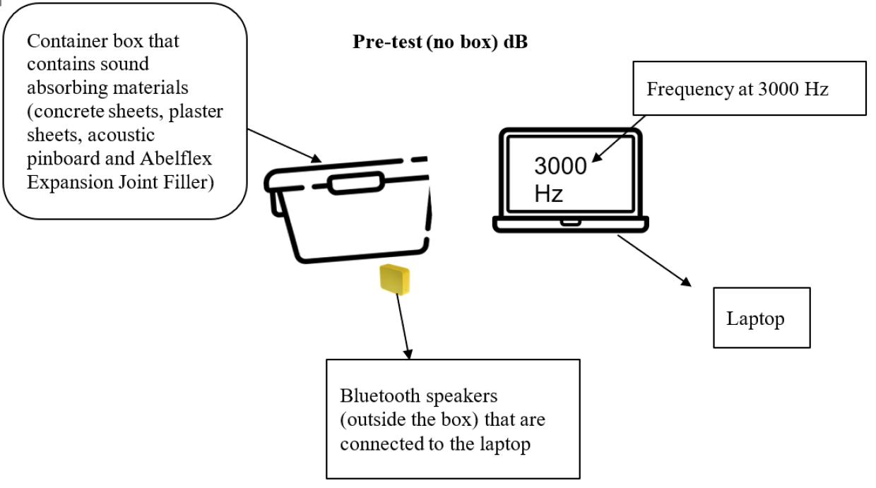
The Journal of Science Extension Research – Vol. 2, 2023 education.nsw.edu.au 214
Preparation of sound – absorbing materials for testing
The following materials and equipment were purchased from Bunnings Australia : x1 Dingo 10kg concrete mix, x2 Dingo 2.5kg Plaster Of Paris, x4 10L Clear Modular Storage Container, x1 Craftright 175mm Gauging Trowel, x1 Small speaker, x1 Computer or laptop, x1 Ormonoid 10 x 150mm 6m Abelflex Expansion Joint Filler, x1 ForestOne 1200 x 800mm 9mm white acoustic pinboard. (note: same thickness is important).
All the statistical analysis was carried out using microsoft excel version 2206. A thorough internet search on tone generator, frequency generator and sound frequency generator was carried out to download. A suitable frequency range of 3000 Hz was selected and downloaded to test. The bluetooth speakers were connected to a laptop. Sound meter app was downloaded from the apple store to measure the frequency of each trial. The selected frequency of 3000 Hz was tested on an empty box container x10 times for reliability then the records were written on a table for the
empty box. Water was added to the cement mixture to turn it into liquid then a trowel was utilized to stick it on each side of the container and let it harden. After the concrete was ready to be tested, bluetooth speakers were placed inside the container. The speaker volume was adjusted to get a constant sound pressure on the sound level meter app at a fixed distance from the speaker. The selected frequency level of 3000 Hz was tested and measured using the “Decibel X” app. The experiment with the concrete sheets was repeated 10x for reliability. Another empty container was out to test the plaster sheets. The plaster mixture was prepared and placed on each side of the container box. Same steps were repeated with the plaster sheets. Third container was also out to examine the acoustic pinboard. The acoustic pinboard was cut out into the same sizes of the container sides, then the same testing steps were repeated with the acoustic pinboard. Finally, the last container was used to examine the Abelflex Expansion Joint Filler and the same steps were also repeated with the Abelflex expansion joint filler. All absorbance data was well processed and organized. an approbating table was made to record the data. Then a column graph was sketched to
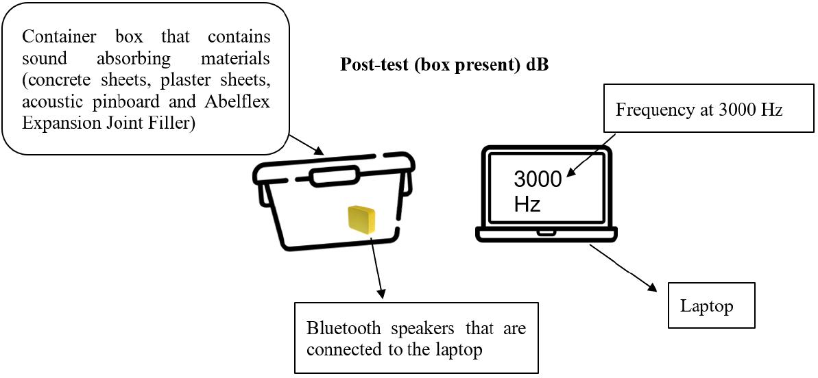
The Journal of Science Extension Research – Vol. 2, 2023 education.nsw.edu.au 215
demonstrate the average results from post and pre tests for each different sound absorbing material was used. A risk analysis was carried out using the RiskAssess software program to find the risks behind conducting this experiment and the risks were such as spill of water, can cause serious injury such as cuts or back, leg injury. In order to prevent this risk, cleaning the area using a mop is required. Loud sounds can cause hearing damage, in order to prevent this issue wear an earplug or keep the speaker volume at a reasonable level.


Results
 Pre-Test (no box) Abelflex Expansion Joint Filter box
Post -Test (Box presence) dB Ablelflex Expansion Joint Filler box
Pre – Test (no box) dB concrete box
Pre-Test (no box) Abelflex Expansion Joint Filter box
Post -Test (Box presence) dB Ablelflex Expansion Joint Filler box
Pre – Test (no box) dB concrete box
The Journal of Science Extension Research – Vol. 2, 2023 education.nsw.edu.au 216
Post – Test (Box presence) dB concrete box
Post

(Box presence) dB concrete


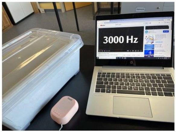

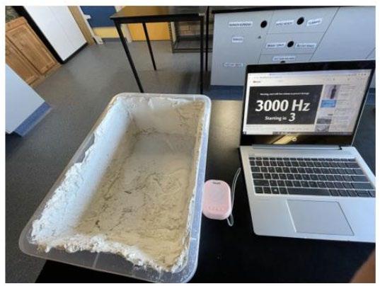
dB
dB
Pre – Test (no box) dB plaster box
– Test
Pre – Test (no box) acoustic pinboard box
Post – Test (Box presence)
acoustic pinboard box
Pre – Test (no box) dB empty box
The Journal of Science Extension Research – Vol. 2, 2023 education.nsw.edu.au 217
Post – Test (Box presence)
acoustic pinboard box
This column graph shows the differences of each sound absorbing materials in order such as ( Acoustic pinboard = blue, Abelflex expansion joint filler = yellow, concrete = red, empty box = purple, and
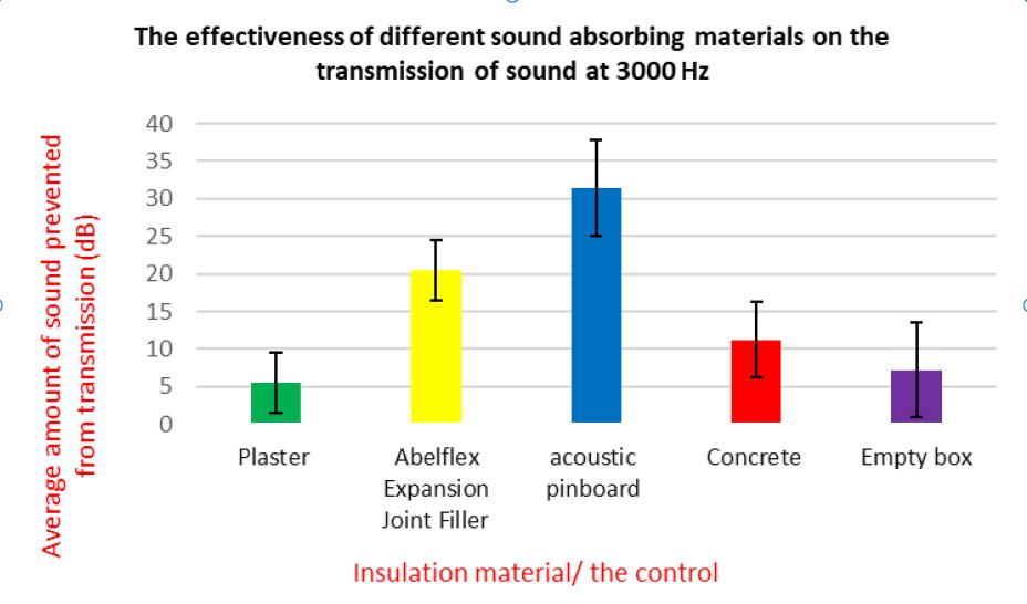
plaster = green). The vertical error bars indicate the standard deviation of each material which was found by the pre-post test averages through using microsoft excel.
The highest standard deviation was 6.431209 with the material acoustic pinboard. Whereas the lowest standard deviation was 3.964509 with the material Abelflex Expansion Joint Filler. As seen in the graph above.
Null hypothesis
For the student's ‘t’ test the null hypothesis stated that there was no difference between the means of the sounds absorption carried out by the materials used. The alternative hypothesis on the other hand stated that the means of the sound absorption carried out by the materials used was not the same. Two sided ‘t’ test was performed with the results shown below:
The Journal of Science Extension Research – Vol. 2, 2023 education.nsw.edu.au 218
This t test table shows the p value difference of each sound absorption material versus empty box to determine the effectiveness of the material. The plaster table shows the P value of 0.4 is greater than the alpha value of 0.05 which means that there is no statistical difference between the exposure of plaster and empty box. The second column table of Abelflex vs empty box shows the P value of 2.7….4E means its highly statistically significant result as alpha value of (0.05) is greater than the p-value. Therefore, the null hypothesis is rejected and hence that homoscedasticity cannot be assumed. Last but not least concrete vs empty box column tables show the P value of 0.1 which is technically greater than the alpha value of 0.05 which means there is no significant difference between the concrete and the empty box. Lastly, acoustic pinboard vs empty box also showed the P value
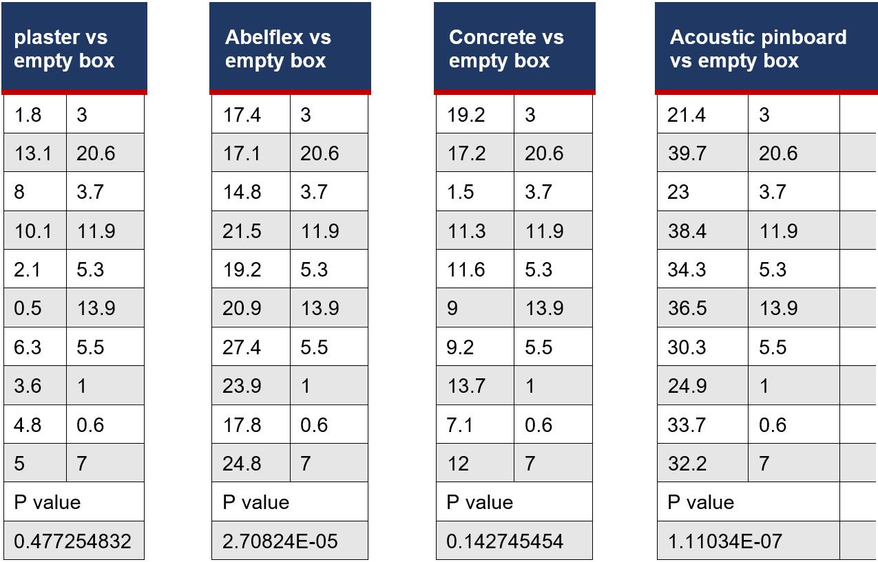
1.1….4E means its highly statistically
significant result as alpha value of (0.05) is greater than the p-value. Therefore, the null hypothesis is rejected and hence that homoscedasticity cannot be assumed.
Table 1-5 demonstrates the sound transmission capabilities of the relevant materials
(concrete sheets, plaster sheets, acoustic pinboard and Abelflex Expansion Joint Filler) at the selected frequency level of 3000 hz. The baseline data of sound transmission was obtained through the absence of the box covered with the relevant material which is shown by the pre test column. The post test column indicates the sound transmission in the presence of the relevant sound absorbing material. The post test data was subtracted from the post test date to find the accurate average transmission capability of the materials used. There were 10 trials carried out with each material and average of the pre test and post test data were taken per material
The Journal of Science Extension Research – Vol. 2, 2023 education.nsw.edu.au 219
used in the investigation. (the higher the average result the better sound absorbing material is).
The order of the best sound absorbing materials was ( acoustic pinboard,
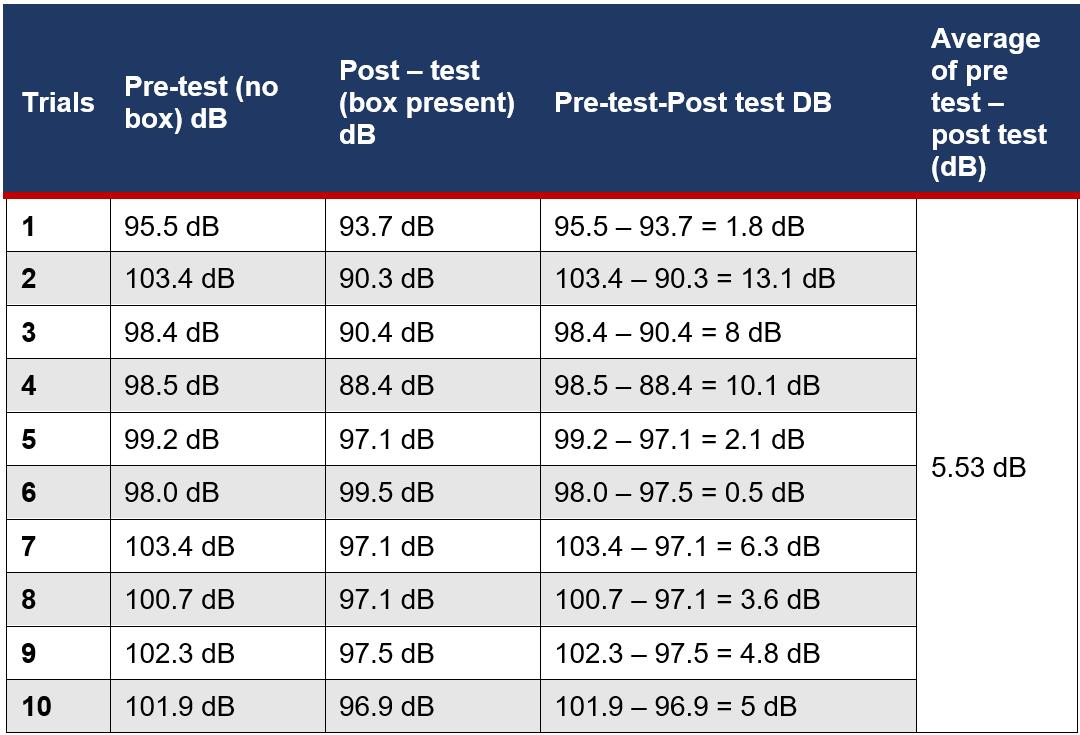 Abelflex Expansion Joint Filler, concrete sheets, empty box, plaster sheets).
The Journal of Science Extension Research – Vol. 2, 2023 education.nsw.edu.au 220
Table 1. Measurement of sound transmittance with the plaster box at 3000 Hz
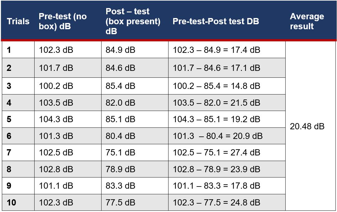
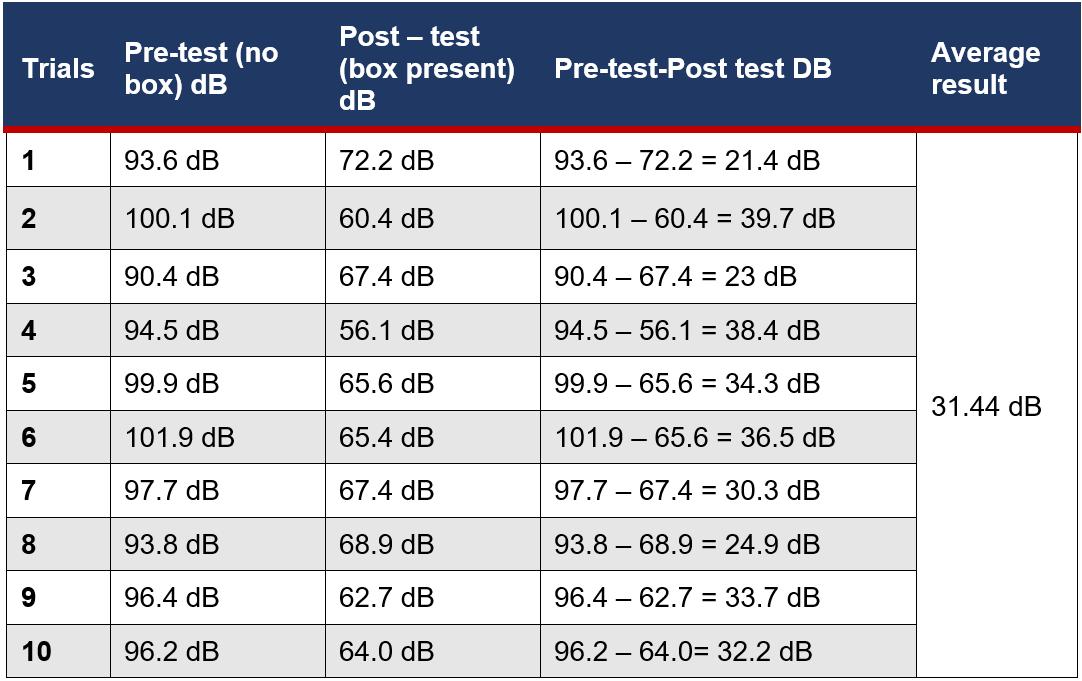 Table 2. Measurement of sound transmittance with the Abelflex Expansion Joint Filler box at 3000 Hz
The Journal of Science Extension Research – Vol. 2, 2023 education.nsw.edu.au 221
Table 3. Measurement of sound transmittance with the white acoustic pinboard box at 3000 Hz

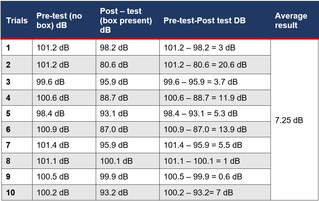 Table 4. Measurement of sound transmittance with the concrete box at 3000 Hz
The Journal of Science Extension Research – Vol. 2, 2023 education.nsw.edu.au 222
Table 5. Measurement of sound transmittance with the empty box at 3000 Hz
Discussion
The following results are presented in the tables to compare the pre test and post test results. The use of the tables and graphs above demonstrates the effectiveness level of each different sound absorption material. The outcome of this experiment reveals that acoustic pinboard was the most effective sound absorption material as it had 31.44 dB average amount of sound prevented from the transmission. Hence the higher result indicates the better sound absorbing material is. The second effective sound absorption material was concrete as it had an average of 20.48 dB. Third highest was Abelflex expansion joint filler as the average was 11.18 dB. Last but not least, the empty box had an average of 7.25 dB and lastly, the plaster had an average of 5.53 dB which means it is the least effective sound transmission material. According to the background research and the literature review the results seemed accurate but the standard deviation shows otherwise. As the acoustic pinboard had a standard deviation of 6.431209 which resulted to be the highest but that means the data is more spread out. Meanwhile the plaster had the lowest standard deviation of 3.949698 and that means the data is
clustered around the mean. As an overall the standard deviation in this experiment was high which indicates that the values are spread out over a wider range. Although the t tests comparing concrete and empty box, plaster and empty box revealed that there was no difference between the high frequency exposed to them. This result needs to be confirmed through further investigations since it is apparent, from literature, that concrete is very dense and thick which makes it an excellent insulator against airborne or impact noises and should work to reflect and absorb sound waves. According to the journal article of “Sound-Absorbing Composites with Rubber Crumb from Used Tires” in their discussion it mentions that “ they have used gypsum and rubber crumb as their sound absorbing material. One can conclude that the most effective in terms of sound absorbing properties is the composition of concrete using only rubber crumb as an aggregate. The result was the composition of concrete using only rubber crumb as an aggregate. The result was achieved due to the addition of the fractioned rubber crumb of fractions from 5 to 2.5 mm in a quantity of 6%; fractions from 2.5 to 1.25 in a quantity of 29%; fractions from 1.25 to 0.63 in a quantity of 29%; fractions from 0.63 from 0.315 to 0.16 mm in a quantity of 7%. The
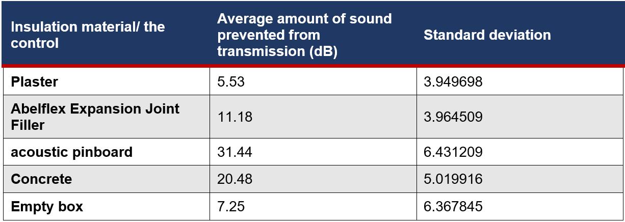 Table 6. The descriptive statistical analysis of the experimental findings
The Journal of Science Extension Research – Vol. 2, 2023 education.nsw.edu.au 223
use of fractioned rubber crumb enables us to obtain the necessary sound absorption since the large specific surface area of open pore walls contributes to the active conversion of sound vibration energy into thermal energy due to friction losses. The use of rubber crumb with larger grains significantly reduces the compressive strength of the developed material. The proposed grain composition of the rubber crumb was stated as a result of evaluating the strength and sound absorption properties of the material. The proposed composite is made from secondary resources, which contributes to the development of resource-and energy-saving technologies. The proposed gypsum–cement–pozzolan composition allows us to increase the sound absorption coefficient, which rises from values of 0.31–0.48 to values of 0.46–0.70 in the studied frequency range in comparison with the composition without rubber crumbs. These results confirm the published data in [43], in which it was shown that the sound absorption coefficient of cement concrete with rubber crumbs increases at high frequencies. Summarizing the results obtained and the previously published data of other authors one can conclude that the sound absorption coefficient of gypsum and cement composites rises significantly with the increase in amount of rubber crumb from used car tires and it depends less on the properties of this rubber crumb. The mechanical properties of gypsum and cement composites significantly depend on both the amount and the properties of the rubber crumb.” Thus in their experimental research the conclusion was “ The use of fractionated rubber crumb allows us to obtain the necessary sound absorption with a less pronounced decrease in strength
characteristics. The proposed grain composition of the rubber crumb was determined as a result of evaluating the strength and sound-absorbing properties of the material. Meanwhile in this experiment the most efficient sound absorption material was the acoustic pinboard. As the acoustic pinboard contains an oven polyester board with a gray finish. It is most likely to be very durable, and absorbs noise with impressive acoustic properties and hence it is an effective pinboard. Therefore the experiment was not accurate nor precise. The experiment requires a lower standard deviation which indicates that the values tend to be close to the mean of the set to be more accurate. This resulted to be one of the limitations in this experiment. The materials used had high SD which affected the precision and consistency of the experiment. When a SD is high, it indicates the precision of the measurement is low which affects the accuracy of the measurement as well. This could be due to the limitation of the methodology used to prevent this more advanced measurement techniques should be used. To improve the low precision it has to be conducted with more trials. For feature direction for scientific research more background research on sound, sound-blocking materials, and sound-blocking construction techniques is required. Then a hypothesis is needed about which materials might be better at attenuating low frequencies, and which materials might be better at attenuating high frequencies. In order to test the hypothesis, it is important to obtain pieces of each of the different materials that are needed to be tested. audio test files also needed and a sound level meter. The audio test files will have a series of pure tones at low, medium, and high
The Journal of Science Extension Research – Vol. 2, 2023 education.nsw.edu.au 224
frequencies. different tones needed to be examined and the sound level meter to test how well the different materials attenuate different frequencies. There were no random mistakes, the results were nearly identical and reflect the true value.
Conclusion
The amount of sound that materials can absorb depends on the frequency of the sound that has been tested. Acoustic pinboard and Abelflex Expansion Joint Filler are lightweight materials and are able to absorb middle and high frequency sounds. As it was hypothesized that when the concrete sheets are tested on the box, they will block more sound transmission than other materials. Hence, acoustic pinboards have polyester which absorbs an impressive amount of sound transmission. Ableflex Expansion Jointing is made from Polyethylene Foam which also absorbs a decent amount of sound. This makes them useful products for controlling sound levels for environments like offices or sound rooms. The use of acoustic pinboard helps to reduce the room’s background sounds, reverberation, echo also it comes in handy on various occasions, including professional recording studios. Soundabsorbing materials are often used in multiple layers to provide compounding effects. The results suggest that these lightweight materials will not work well to control higher energy, low-frequency bass waves. Therefore the performance of the soundproof foam depends on the type of foam used and its efficiency in absorbing and dissipating the sound energy into heat energy. Future investigations need to confirm the findings from this study.
Reference list
Soundproof Cow. 2021. What is Sound? The Science of Sound | Soundproof Cow. [online] Available at: <What is Sound? The Science of Sound | Soundproof Cow> [Accessed 8 December 2021].
Soundproof Cow. 2021. How Noise Affects Individuals with Autism | Soundproof Cow. [online] Available at: < How Noise Affects Individuals with Autism | Soundproof Cow> [Accessed 8 December 2021].
Perfect Acoustic. 2021. AcousticsImportance of acoustic. [online] Available at: < Acoustics - Importance of acoustic (perfectacoustic.co.uk)> [Accessed 8 December 2021].
Google.com. 2021. Before you continue to Google Search. [online] Available at: <https://www.google.com/search?q=why+ is+acoustic+sound+absorbing+material s+importnat&rlz=1C1GCEA_enAU980AU 980&ei=jOinYaj6EtSfseMPlpmJoA4&ve d=0ahUKEwio8JuhxcP0AhXUT2wGHZZ MAuQQ4dUDCA4&uact=5&oq=why+is+ acoustic+sound+absorbing+materials+im portnat&gs_lcp=Cgdnd3Mtd2l6EAMyB wghEAoQoAE6BAgAEEc6BQghEKABOg QIIRAVOggIIRAWEB0QHjoGCAAQFh AeSgQIQRgAUO4KWK64AmCDugJoA3 ADeAGAAdACiAGESpIBCTAuMTYuMj YuMpgBAKABAcgBCMABAQ&sclient=gw s-wiz > [Accessed 8 December 2021].
Science Buddies. 2021. FrequencyDependent Sound Absorption | Science Project. [online] Available at: <https://www.sciencebuddies.org/science -fair-projects/projectideas/Phys_p029/physics/frequencydependent-sound-absorption#background > [Accessed 8 December 2021].
Soundproof Living. 2021. 14 Best Sound Absorbing Materials for Home and Studio
The Journal of Science Extension Research – Vol. 2, 2023 education.nsw.edu.au 225
Acoustics. [online] Available at: <https://soundproofliving.com/list-ofsound-absorbing-materials/ > [Accessed 8 December 2021].
Fields, A., 2021. Best Sound Absorption Materials - www.AcousticFields.com. [video] Available at: https://www.youtube.com/watch?v=nUiwh AmaJME > [Accessed 8 December 2021].
can?, W., Dey, S. and Rennie, J., 2021. Why can't light pass through walls but sound can?. [online] Physics Stack Exchange. Available at: <https://physics.stackexchange.com/ques tions/37823/why-cant-light-pass-throughwalls-but-sound-can > [Accessed 8 December 2021].
Quora. 2021. Why does sound go through walls?. [online] Available at: <https://www.quora.com/Why-doessound-go-through-walls > [Accessed 8 December 2021].
CertainTeed. 2021. How to Reduce Noise in Any Room. [online] Available at: <https://www.certainteed.com/soundadvice-when-where-how-to-reduce-noise/ > [Accessed 8 December 2021].
Akoustix. 2021. Types of Sound Transmission. [online] Available at: <https://www.akoustix.co.uk/blogs/akousti x-university/types-of-sound-transmission > [Accessed 8 December 2021].
Ritzo, M., 2021. How to Soundproof: Acoustic Foam Does Not Block Sound. [online] Acoustical Solutions. Available at: <https://acousticalsolutions.com/how-tosoundproof-acoustic-foam-does-notblock-sound/ > [Accessed 8 December 2021]
Munk, W., O'Reilly, W. and Reid, J., 2021. Australia-Bermuda Sound Transmission Experiment (1960) Revisited. [online] AMETSOC. Available at:
<https://journals.ametsoc.org/view/journal s/phoc/18/12/15200485_1988_018_1876 _abster_2_0_co_2.xml> [Accessed 8 December 2021].
Teach Me Audio. 2021. Audio Spectrum. [online] Available at:
<https://www.teachmeaudio.com/mixing/t echniques/audio-spectrum > [Accessed 8 December 2021].
It's a Noisy Planet. Protect Their Hearing. 2021. How is Sound Measured?. [online]
Available at:
<https://www.noisyplanet.nidcd.nih.gov/h ave-you-heard/how-is-sound-measured> [Accessed 8 December 2021].
Instrument Choice.com.au. 2021. How Do You Measure Noise Levels?. [online]
Available at:
<https://www.instrumentchoice.com.au/ne ws/how-do-you-measure-noise-levels> [Accessed 8 December 2021].
Iancommunity.org. 2021. What Do We Know about Noise Sensitivity in Autism? |Interactive Autism Network. [online]
Available at:
<https://iancommunity.org/ssc/noisesensitivity-autism> [Accessed 8 December 2021].
Autism Speaks. 2021. Autism and Anxiety: Loud Noises | Autism Speaks. [online] Available at:
<https://www.autismspeaks.org/expertopinion/autism-and-anxiety-loud-noises> [Accessed 8 December 2021].
Soundproof Cow. 2021. Sound Absorbing Materials - Premium Sound Absorption |
The Journal of Science Extension Research – Vol. 2, 2023 education.nsw.edu.au 226
Soundproof Cow. [online] Available at: <https://www.soundproofcow.com/produc t-category/sound-absorption-materials/>
[Accessed 8 December 2021].
Snoring Source. 2021. Sound Absorbing Materials: Types and How They Work!Snoring Source. [online] Available at: <https://www.snoringsource.com/soundabsorbing-materials/> [Accessed 8 December 2021]
Iopscience.iop.org. 2022. ShieldSquare Captcha. [online] Available at: <https://iopscience.iop.org/article/10.1088 /1742-6596/908/1/012005/meta >
[Accessed 1 September 2022].
The Journal of Science Extension Research – Vol. 2, 2023 education.nsw.edu.au 227
Disproving the misconception that microscopic black holes can expand
Surabhi Hebbar Blacktown Girls High School
This report disproves the common misconception that microscopic black holes produced in supercolliders would expand and absorb matter until it grew to the size of a cosmic black hole. This is done by deriving Hawking’s equations from his 1975 paper using dimensional analysis and observing the relationship between the variables of mass and time to evaporation. It showed that as mass increases the time to evaporation also greatly increases (�������������������� = 10 16 × ����3 ). This shows that microscopic black holes cannot expand as it releases energy too quickly and evaporates to be able to absorb energy. Therefore, there is no time for microscopic black holes to start accreting matter to the size of a cosmic black hole. The impact of this area of research can lead to new discoveries and development of technologies that will advance our knowledge and understanding of the universe.
Literature review
The nature of microscopic black holes is still under ongoing research, however, basic knowledge about their lifetime and mass-energy properties can be understood. Contrary to common belief, a microscopic black hole cannot expand like a cosmic black hole would, due to its very small mass or energy.
Misunderstandings of the production of a microscopic black hole in the Large Hadron Collider (LHC) caused a legal battle between CERN and critics.
According to Lisa Zyga (2010), in May of 2008 a lawsuit was filed against the operation of the LHC based on the concern that the LHC would produce a black hole that could expand and destroy the Earth. Although this lawsuit concluded that there are no potential adverse effects of the operation of the LHC, many people are concerned with the experiments conducted in the LHC (Johnson, 2009).
Thus, it is required to examine the nature of black holes, cosmic and microscopic to better understand the relationship between their mass and lifetime to disprove that microscopic black holes can expand.
Particle accelerator/collider
A particle accelerator or collider is a machine that uses electromagnetic fields to direct and accelerate charged particles to speeds close to the speed of light (CERN, 2022). The particles are accelerated into beams that travel in opposite directions in the ring, then they collide with one another, and the effect is observed and analysed. A microscopic black hole forms when two particles travelling the same plane as they do in the LHC have almost reached each other. However, observing these phenomena is very difficult due to their volatile nature and the difficulty in producing and containing one (Cavaglià, 2010).
The Journal of Science Extension Research – Vol. 2, 2023 education.nsw.edu.au 228
Microscopic black hole
A microscopic black hole is a very small black hole that can be produced by highenergy collisions of protons in protonproton (p-p) collision. The black hole produced would be smaller than the size of an atom (Khachatryan, 2011). A Schwarzschild black hole is the simplest form of a black hole, as they are only defined by their mass i.e., they have no electric charge or spin (Xiao, 2020). The main issue with trying to observe the nature of microscopic black holes is that they have very small lifetimes, making it difficult to observe any of their properties (CERN, 2022).
The common misconception
The common misconception about the microscopic black hole is that it will continue to expand and consume matter similar to cosmic-sized black holes. However, this is not the case, as once a microscopic black hole is produced it would decay thermally via Hawking radiation (Hawking, 1975). The time taken for black holes to evaporate can be calculated through dimensional analysis and used to understand the relationship between mass and time to evaporation.
Cosmic Black Holes
Cosmic Black holes are categorised based on size. Stellar Black holes are the smallest weighing a few solar masses, these black holes were large stars that collapsed onto themselves. Intermediate black holes were large stars or smaller primordial black holes. Supermassive black holes are primordial black holes that have huge masses (Gebhardt, 2013). Cosmic black holes are used to investigate the relationship between mass and time to evaporation as they can be
better observed and studied as they have a greater lifetime. They are also used to prove using real data that microscopic black holes have a very short lifetime.
Deficiencies in the evidence
Research into the nature of cosmic black holes has been extensively advanced by the work of Stephen Hawking in his 1975 paper Particle Creation by Black Holes, and later extended to the general public in more simple terms in his novel A Brief History of Time. Despite this, there is little published to the public to examine the nature of microscopic black holes. The experiments conducted by CERN (2022) and other research into quantum mechanics and black holes (Xiao, 2020) are still ongoing and uncertain as to the nature and properties of the micro black hole. There is also a lack of observable proof that microscopic black holes cannot expand, this paper attempts to find proof in cosmic black holes to explain the nature of microscopic black holes.
There are many speculations about what we could achieve by harnessing a microscopic black hole, among which are time travel into the past and proving existing theories like string theory. The impact of understanding its nature opens many pathways for study and technological progress in the future. This report also helps improve the understanding of microscopic black holes to the reader by disproving their misconceptions, allowing them to be assured there is no danger in experimenting with microscopic black holes.
The Journal of Science Extension Research – Vol. 2, 2023 education.nsw.edu.au 229
Hawking radiation and temperature
Hawking radiation is thermal radiation that is theorised to be emitted from black holes. It is emitted from the region of space surrounding the event horizon. Although it hasn’t been observed it has been widely accepted in the scientific community (Kováčik, 2021)
Hawking temperature is the temperature of the thermal radiation emitted from a black hole. Since, mass and energy are seen as equivalent according to Einstein’s famous equation, E=mc^2. By that logic when a black hole radiates energy, it also loses mass and should eventually evaporate (Johnson, 2009).
Dimensional analysis of Hawking equations
Dimensional analysis is a problem-solving method that uses the fact that any number or value can be multiplied by one without changing its value. It is used to analyse the relationship between different quantities. This method is used to derive a more simplified version of Hawking’s equations that display the relationship between the variables associated with a black hole, in this case, will be its mass and time to evaporation (LoPresto, 2003). It is not able to derive its product constants, however, this is unnecessary to understand the relationship between mass and time to evaporation.
Scientific research question
To what extent is there a relationship between mass and time to evaporation of black holes?
Aim
The aim of the research is to disprove the misconception that a microscopic black hole of small mass produced in a supercollider can expand its event horizon and gain mass until its gravitational force is enough to grow into a cosmic black hole.
Scientific Hypothesis
There is a significant correlation between the mass and time to evaporation of black holes, such that as the mass of a black hole increases so will the time to evaporation. Therefore, a microscopic black hole will have a very small lifetime as it will evaporate in a very short time due to its extremely small mass/energy. It cannot absorb mass/energy and grow, as it will in fact emit energy in the form of Hawking radiation.
Methodology
The method of dimensional analysis was used to derive an equation with variables of mass and time to evaporation. To simplify the calculations a Schwarzschild black hole is considered. In the case of particle accelerators forming black holes, it cannot produce a Schwarzschild black hole as the collision between two charged particles will inevitably cause the black hole to become electrically charged (a particle accelerator cannot accelerate neutral particles, as it uses the electric and magnetic fields). However, for the purpose of analysing only the mass of black holes and their correlation to
The Journal of Science Extension Research – Vol. 2, 2023 education.nsw.edu.au 230
evaporating time its charge can be disregarded for simplicity. This would have no effect on the analysis between variables, but rather the accuracy of the physical values, as they are not being calculated they can be consciously discarded. A regression/correlation test is then conducted between black hole mass and time to evaporation using a secondary source of cosmic black hole masses (Gebhardt, 2013) to observe if there is a significant correlation between the mass and time to evaporation of black holes. This secondary data was taken from the University of McDonald Texas Observatory.
Materials
The materials required to carry out this experiment are a scientific calculator, secondary data source from the University of McDonald Texas Observatory and Excel spreadsheets.
Design
The experimental design is a regression correlation study to measure the statistical correlation between mass and time to evaporation of black holes. Then the paired t-statistic was used to calculate the p-value, with a confidence level of 95% to determine its significance.
Procedure
Deriving Hawking Equation(s) using Dimensional Analysis.

The Journal of Science Extension Research – Vol. 2, 2023 education.nsw.edu.au 231
Discard 2 3 in dimentional analysis (just a constant),
N is no of atoms (constant, also discard)
Area of Event Horizon:
Black holes are massive, involve speed of light (M,G,C)
The area of Event Horizon increases with mass ����∝����2
The actual Formula for Area of Event Horizon (constant of 16π):
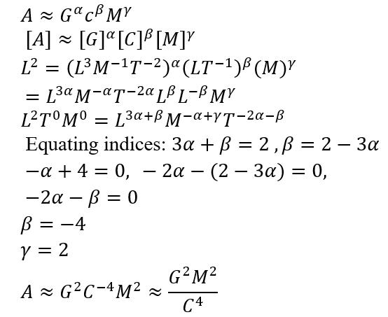

According to classical physics nothing can escape from the event horizon, as a velocity greater than C is needed. Thus, the area of a black hole can only increase (2nd law of thermodynamics).
Black Hole Entropy:
Entropy of an isolated system must increase with time (cannot decrease)
���� = 16�������� 2 ����2 ���� 4
The Journal of Science Extension Research – Vol. 2, 2023 education.nsw.edu.au 232
Exact equation for entropy (with constant
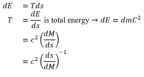
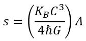
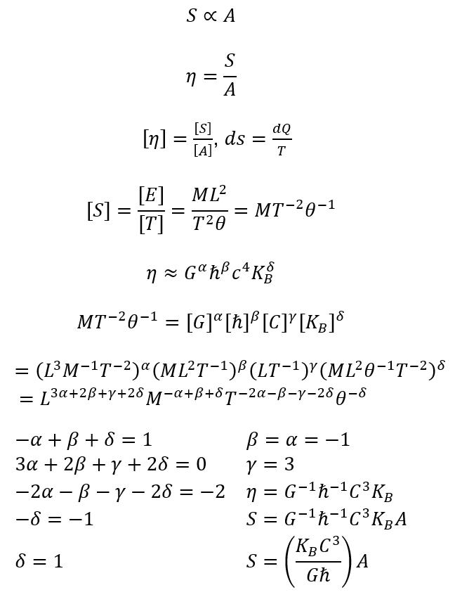
S is very large as ���� 3 is in numerator and ℏ and ���� in denominator.
1 st Law of thermodynamics
�������� = �������� + ��������
2 nd Law of thermodynamics
�������� = �������� ����
Assuming black hole does no work on its surroundings, �������� = 0
1 4)
The Journal of Science Extension Research – Vol. 2, 2023 education.nsw.edu.au 233
Differentiate black hole entropy with respect to mass.
Equate powers
Time taken for a Black Hole to Evaporate:
���� is time
���� is power
���� is energy
���� is area ����
Power emitted per unit area from object of temperature
Real equation (with constant
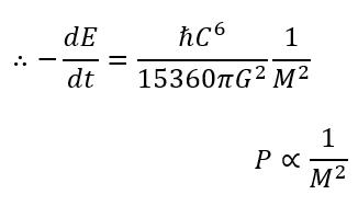
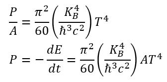
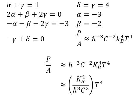
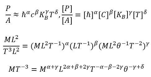
(derived using entropy of black hole)
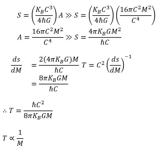
���� ����
= ���� ����
=
����
����
����2 60
���� = 16�������� 2 ����2 ���� 4 ,
���� = ℏ���� 2 8������������ ��������
The Journal of Science Extension Research – Vol. 2, 2023 education.nsw.edu.au 234
): Sub
and entropy equation for temperature
The smaller the mass the greater the Power output or energy released
∴ smaller the mass, smaller the evaporation time.
Consider a microscopic black hole of mass of 2 protons ≈ 3.346 × 10 27
�������������������� = 10 16 × (3.346 × 10 27 )3 =3.746 × 10 96 s.
where ���� = �������������������� → Moment in time where mass of black hole is reduced to 0,
The equation for time to evaporation (�������������������� = 10 16 × ����3 ) was then used to calculate the time to evaporation for various cosmic black holes (stellar, intermediate, and supermassive). The masses of these black holes were then substituted into the derived equation to obtain a value for the time taken for the black hole to evaporate. These values were recorded in a table and a regression/correlation test was run to determine the r-value, t-score, and pvalue between the dependent variables of mass and time to evaporation.
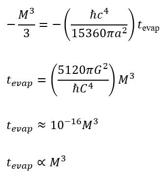
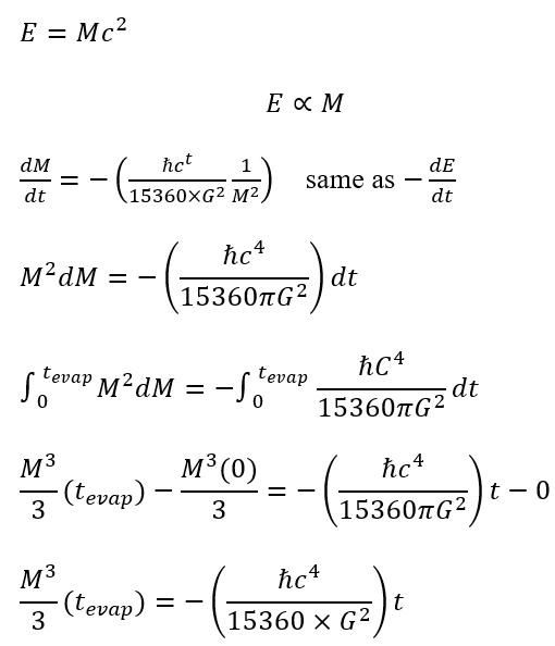
The Journal of Science Extension Research – Vol. 2, 2023 education.nsw.edu.au 235
The trend line is linear with ���� 2 value of 0.847 and correlation coefficient (r) is 0.9205. The error bars show standard error of data. T-statistic of 16.99 was calculated and P-value of 0.0174 (less than 0.05) was obtained. Therefore, data is statistically significant.
Discussion
The data shown in figure one shows an exponential relationship where, as the mass of black holes increases, the time to evaporation also increases exponentially. This trend is confirmed through dimensional analysis, it is shown that the time to evaporation is proportional to the mass cubed, which explains that as the mass increases slightly the time to evaporation increases much greatly. The correlation coefficient (r) is 0.9205 which shows that the graph has a strong and positive correlation between variables.
Thus, there is a clear correlation between the mass of black holes and their time to evaporation. There is also a causation between them, as proved through dimensional analysis, the relationship between mass and temperature showed that the smaller the black hole the greater the temperature. In addition, the time to evaporation is related to the temperature of the black hole, where the higher the temperature the shorter the time to evaporation. The results from the experiment confirmed the hypothesis, as there was a relationship between black hole mass and time to evaporation that
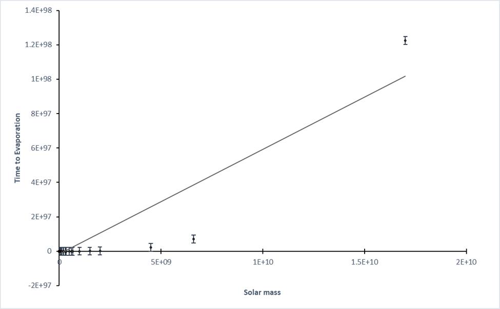
Results
Figure 1: Graph of the relationship between mass and time to evaporation of black holes.
Note: This figure demonstrates the relationship between the variables of mass and time to evaporation of black holes using 54 data points.
The Journal of Science Extension Research – Vol. 2, 2023 education.nsw.edu.au 236
was statistically significant as the p-value is less than 0.05.
Since energy and mass are essentially equivalent as Einstein showed in his famous equation ���� = �������� 2 , then a black hole emitting Hawking radiation is a black hole that is losing mass. Black holes have a temperature that varies inversely with their mass and so large black holes would be extremely cold and would radiate energy extremely slowly. Conversely, the smaller the black hole, the greater the temperature and the faster it would radiate energy. The faster that energy is radiated the faster its evaporation rate becomes. Thus, microscopic black holes of a mass of approximately two protons (3.346×10 27 kg), will have an evaporation time proportional to its mass cubed, which is extremely fast (3.746× 10 96 ����) shown through dimensional analysis. Therefore, a microscopic black hole would be unable to absorb mass, as its evaporation time is too fast. Therefore, microscopic black holes cannot be compared to a cosmic black hole and will evaporate very quickly. These findings are verified by various literature published by CERN 2022 on their website and previous research conducted on microscopic black holes (LoPresto, 2003). In addition, Stephen Hawking’s published work in 1975 confirms equations derived through dimensional analysis. This further verifies the validity and accuracy of the experiment conducted and the results obtained from the investigation.
Figure 1 mainly shows that larger supermassive black holes, and the smaller mass black holes have very close data points at the bottom. This shows the large range of the time to evaporation of these black holes, indicating that a change in mass had a great effect on the
time to evaporation of black holes. However, due to the large range of values the graph cannot display all the values accurately and is forced to increase with larger increments on the y-axis. This reduced the accuracy of the graph when viewed and made it more difficult to observe the linear relationship without referring to the correlation coefficient. Despite this, the systematic errors are minimised as results received from investigation are confirmed with existing data from a Hawking radiation calculator (Toth, 2016). Validity and accuracy were maintained as there was a sufficient number of data points (n=54), the systematic errors were minimised, statistical tests used were appropriate and results were confirmed. Random errors have been accounted for in error bars on the graph, however, the experimental procedure conducted would have minimised the extent of the errors, as the calculations were conducted through Excel Spreadsheets and data taken from a reputable secondary source (Gebhardt, 2013), improving the precision of the data. The experiment was reliable as a correlation was found between the variables over multiple data points and this relationship was consistent across the data points.
This research report was able to successfully accept the hypothesis and conclude that microscopic black holes cannot expand by deriving and providing both theoretical and experimental proof to support the hypothesis. However, the limitation of the experiment was the method of derivation used. Dimensional analysis is not completely accurate and requires the constants derived using quantum physics to complete the process, however, it was reasonably close. The report was able to disprove the
The Journal of Science Extension Research – Vol. 2, 2023 education.nsw.edu.au 237
misconception that microscopic black holes can expand to the public audience and combined areas of research in quantum theory, particle physics, and astronomy by comparing the nature of cosmic black holes with microscopic black holes. This comparison provided a unique understanding of why microscopic black holes do not expand but cosmic black holes do, disproving the danger of creating microscopic black holes. The future directions of this research are analysing microscopic black hole signatures to uncover further qualities of microscopic black holes. Methods such as mathematical simulations and energy readings from the LHC can further build upon the research into microscopic black holes. Research into this area is beneficial for the technological advancement and study of black holes in space.
Conclusion
In summation, this report disproved the common misconception that microscopic black holes produced in supercolliders would expand and absorb matter until it grew to the size of a cosmic black hole. This was done by deriving Hawking’s equations from his 1975 paper using dimensional analysis and observing the relationship between the variables of mass and time to evaporation. Furthermore, the mass of cosmic black holes was used to demonstrate the relationship between mass and time to evaporation and showed that as mass increases that time to evaporation also greatly increases. This unique comparison between cosmic black holes to microscopic black holes showed the differences in their properties, as microscopic black holes have a very short lifetime compared to cosmic black holes to cause any macroscopic effects. The limitation of the report is the accuracy of dimensional analysis, as without the knowledge of quantum physics the derived equations do not have accurate constants. The future of research into black holes can be built upon our understanding of microscopic black holes and their properties can be used in technologies that could revolutionise our society.
References
Cavaglià, M. (2010). Particle accelerators as black hole factories? « EinsteinOnline. Einstein-online.info. Retrieved 24 August 2022, from https://www.einsteinonline.info/en/spotlight/accelerators_bh/
The Journal of Science Extension Research – Vol. 2, 2023 education.nsw.edu.au 238
Gebhardt, K. (2013). Supermassive black holes directory - StarDate's Black Hole Encyclopedia. Blackholes.stardate.org. Retrieved 24 August 2022, from http://blackholes.stardate.org/objects/type -supermassive.html
Hawking, S. (1975). Particle creation by black holes. Communications In Mathematical Physics, 43(3), 199-220.
https://doi.org/10.1007/bf02345020
Johnson, Eric.E. (2009). The Black Hole Case: The Injunction Against the End of the World. Vol. 67, Pg. 820-849.
https://doi.org/10.48550/arXiv.0912.5480.
Khachatryan, Vardan & Sirunyan, Albert & Tumasyan, Armen & Adam, Wolfgang & Bergauer, Thomas & Dragicevic, Marko & Erö, Janos & Fabjan, Christian & Friedl, Markus & Frühwirth, Rudolf & Ghete, Vasile & Hammer, Josef & Haensel, Stephan & Hartl, Christian & Hoch, Michael & Hörmann, Natascha & Hrubec, Josef & Jeitler, Manfred & Kasieczka, Gregor & Weinberg, Marc. (2011). Search for Microscopic Black Hole Signatures at the Large Hadron Collider. Physics Letters B. 697. 434. 10.1016/j.physletb.2011.02.032.
Kováčik, S. (2021). Hawking-radiation recoil of microscopic black holes. Vol 34, Pg. 1.
https://doi.org/10.1016/j.dark.2021.10090
6
LoPresto, M. (2003). Some Simple Black Hole Thermodynamics. The Physics Teacher, 41(5), 299-301.
https://doi.org/10.1119/1.1571268.
The Safety of the LHC | CERN. Home.cern. (2022). Retrieved 24 August 2022, from
https://home.cern/science/accelerators/lar ge-hadron-collider/safety-lhc
Toth, V. (2016). Viktor T. Toth - Hawking radiation calculator. Vttoth.com. Retrieved 24 August 2022, from https://www.vttoth.com/CMS/physicsnotes/311-Hawking-radiation-calculator.
Xiao, Y. (2020). Microscopic derivation of the Bekenstein-Hawking entropy for Schwarzschild black holes. Physical Review D, 101(4).
46 020.
Zyga, L. (2010). LHC lawsuit case dismissed by US court. Phys.org. Retrieved 24 August 2022, from https://phys.org/news/2010-09-lhclawsuit-case-dismissed-court.html
https://doi.org/10.1103/physrevd.101.0
The Journal of Science Extension Research – Vol. 2, 2023 education.nsw.edu.au 239
Predicting Solar Proton Event Magnitudes Using Vector Magnetic Data and a Neural Network Title of article
Vincent Ng
James Ruse Agricultural High School
This study aimed to create and evaluate a neural network using vector magnetic data to predict the maximum proton flux at Earth caused by a future solar proton event (SPE), in which protons are accelerated to near-relativistic energies by solar eruptions. Two bidirectional long short-term memory (biLSTM) neural networks were developed to investigate the SPEs in the NASA/NOAA Solar Energetic Proton List. Both networks used data samples obtained from the Spaceweather HMI Active Region Patches (SHARPs) as input, however, the maximum proton flux of SPEs outputted was linearly scaled in one network and logarithmically scaled in the other. By analysing the ratio of underestimations to overestimations and comparing the error of the predictions made by these neural networks to the corresponding errors for baseline models with no skill, it was evident that the neural networks created in this study were not sufficiently accurate to be used for realworld applications.
Introduction
Solar proton events (SPEs) occur when protons are accelerated to nearrelativistic energies by solar eruptions. These events generate a flux of protons, measured in proton flux units (pfu), which may be directed at the Earth. The SWPC (Space Weather Prediction Centre) defines the start time of an SPE as the first of three consecutive data points where the flux of protons with energies greater than 10 MeV as measured by the Geostationary Operational Environmental Satellites (GOES), which orbit the Earth, is at least 10 pfu (National Oceanic and Atmospheric Administration [NOAA] 2022). SPEs can cause damage to the technical systems of space probes outside Earth’s magnetosphere and produce radiation which may be lethal to astronauts and affect passengers and flight crews on polar airline routes.
Additionally, large SPEs can ionise, excite, and dissociate atoms and molecules in the atmosphere, which can lead to ozone depletions in the polar upper stratosphere (Schwenn 2006).
Researchers have approached the problem of SPE prediction by developing empirical models with varying inputs. SPEs correlate with coronal mass ejections (clouds of ionised gas ejected from the Sun) and solar flares (sudden bursts of electromagnetic radiation emitted by the Sun) (Anastasiadis et al. 2019), so empirical prediction models have been developed using solar flare and coronal mass ejection data. For example, the ESPERTA model uses the flare location and soft x-ray and radio fluence (total amount of radiation flowing through an area) data, up to 10 minutes after the soft x-ray flux peak corresponding to a solar flare, to predict the probability of an SPE (Laurenza et al.
The Journal of Science Extension Research – Vol. 2, 2023 education.nsw.edu.au 240
2018). Núñez et al. (2019) found that the UMASEP scheme, which predicts SPEs using the correlation between the intensity of soft x-rays emitted by the Sun and the differential proton fluxes (rate of proton flow through an area) measured near the Earth, could be adapted to take the intensity of extreme ultraviolet radiation as input. Núñez et al. (2020) built the UMASOD model, a decision tree model using flare and radio burst observational data to make a binary prediction on whether an SPE is expected. The most important attributes for this model were the soft x-ray fluence, the flare’s heliolatitude, and the maximum frequency of the type III radio bursts (radio emissions from the Sun associated with solar flares)
SPEs are affected by the Sun’s vector magnetic field because they occur when protons are accelerated by the energy release processes associated with the evolution of the Sun’s three-dimensional magnetic structure. Furthermore, these accelerated protons tend to move along the magnetic field lines emanating from the Sun because they are subject to the magnetic component of the Lorentz force, which acts on charged particles with a component of velocity directed perpendicularly to the local magnetic field (Vlahos 2019). Abduallah et al. (2022) developed a bidirectional long short-term memory (biLSTM) neural network to make a binary prediction of whether a solar Active Region (AR) would produce a SPE using data from the Spaceweather HMI Active Region Patches (SHARPs).
SHARPs contain physical parameters describing the nature of the vector magnetic field within the Sun’s Ars
Whilst there have been predictive models developed to make binary or probabilistic
predictions of whether an SPE will occur, there are fewer models designed to predict the maximum proton flux associated with a future SPE, and none using vector magnetic data. It would be useful to predict the maximum proton flux experienced at Earth because this determines the impact of an SPE on Earth, as outlined by the NOAA S-Scale (Appendix 1). For example, an S1 (minor) SPE is unlikely to have any biological or technological impacts, however, an S5 (extreme) SPE will expose astronauts outside space vehicles to high doses of radiation and may render satellites useless (NOAA n.d.). Therefore, the aim of this study is to create a neural network using vector magnetic data to predict the maximum proton flux experienced at Earth as a consequence of a future SPE. In practice, this predictive model would be used after another model has made a binary or probabilistic prediction indicating that an SPE is likely to occur
Scientific Research Question
Can vector magnetic data from the Sun’s ARs be used to predict the maximum solar proton flux that could be experienced at Earth as a consequence of a future SPE that will occur within the subsequent 24 hours?
The Journal of Science Extension Research – Vol. 2, 2023 education.nsw.edu.au 241
Methodology
Constructing the Dataset
The NASA/NOAA Solar Energetic Proton List was used to create a database of SPEs that occurred from 1 May 2010 onwards, the date that the Helioseismic and Magnetic Imager (HMI) began collecting vector magnetic data. This database contained the start and maximum time, maximum proton flux, and NOAA AR for each SPE.
Vector magnetic data was obtained from the Spaceweather HMI Active Region Patches (SHARPs) created by Bobra et al. (2014), which is a data time series that documents 15 physical parameters of ARs with a 12-minute cadence (Figure 1, Appendix 2). These parameters are derived from the vector magnetograms taken by the HMI.
SPEs were omitted from the database of events if they were missing values for the start or maximum time, the maximum proton flux, or the NOAA AR. Additionally,
SPEs were omitted if SHARP physical parameters could not be collected for at least 10 consecutive timesteps (points in time with data recorded). This reduced the number of events in the period 1 May 2010 to 30 June 2022 from 42 to 35 (Figure 4).
SHARP physical parameters from the AR associated with each SPE were collected for the 24 hours leading up to the event (Figure 2a). Given that the SHARP physical parameters have a 12-minute cadence, it was expected that there would be 120 timesteps for a 24-hour period, and thus 4200 timesteps for the 35 events investigated. However, because some ARs did not have data available for the entire 24-hour period preceding the event, there was only data for 3961 timesteps. This simulates how a neural network operating in real-life conditions may not have access to data for the full 24-hour period preceding a future SPE whose magnitude is to be predicted (Figure 2b).
The Journal of Science Extension Research – Vol. 2, 2023 education.nsw.edu.au 242
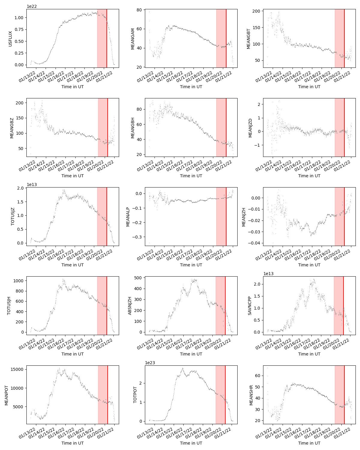
The Journal of Science Extension Research – Vol. 2, 2023 education.nsw.edu.au 243
Figure 1: Plot of the fifteen SHARP physical parameters over time for the NOAA AR 2929 from 12 January 2022 10:36 UTC to 21 January 2022 00:36 UTC. The start time of the SPE (20 January 2022 08:00 UTC) (red line) and the 24-hour period leading up to it (red shaded area) have been added, using data from the NASA/NOAA Solar Energetic Proton List.
Figure 2: For each SPE, the neural network used the SHARP physical parameters from the associated AR for the 24 hours leading up to it. (a) When data was available beyond the 24 hours before the SPE, only the data from the 24 hours leading up to the SPE were considered. (b) When data was not available for the entire 24 hours leading up to the SPE, all data from timesteps preceding the start time of the SPE were considered.
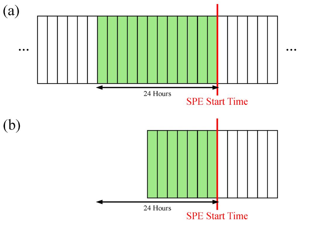
Data samples were created from the SHARP physical parameters from 10 consecutive timesteps (Figure 3a), following the methodology used by Abduallah et al. (2022). These data samples were stored as 10×15 arrays (Figure 3b) to ensure that the inputs to the neural network had consistent data dimensions. The data samples overlapped with each other, meaning that each timestep formed part of multiple data samples. This ensured that the neural network could learn the relationships between consecutive timesteps, given that neural networks can only learn the relationships between the timesteps contained within a single data sample.
All data samples were stored in a single array to be inputted into the neural network. Each data sample was paired with its corresponding target value, the actual maximum proton flux measured for each SPE, which occupied the same
index as the data sample in a second array containing the target values (Figure 3c).
Figure 3: (a) The data samples were created from the 15 SHARP physical parameters from 10 consecutive timesteps and overlapped with each other, so each timestep formed part of multiple data samples. (b) Each data sample was stored as a 10×15 array, with the first dimension corresponding to the 10 timesteps, and the second dimension corresponding to the 15 SHARP physical parameters. (c) The data samples and the target maximum proton flux values were each stored in an array. The data sample and target value for each SPE were paired by storing them in the same index in the respective array.
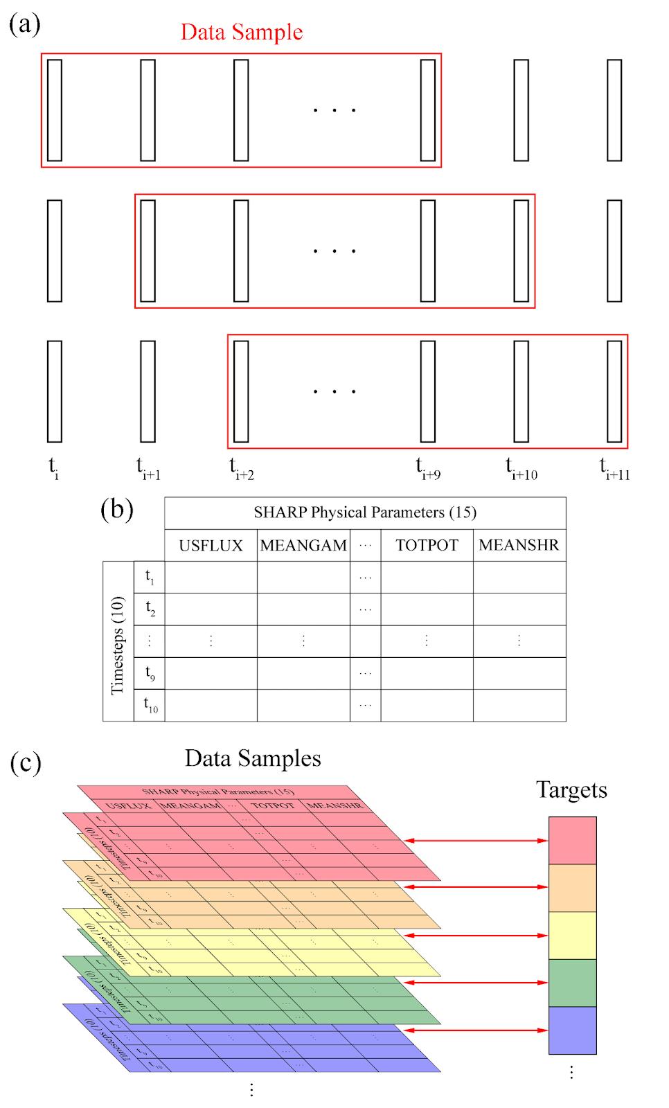
The Journal of Science Extension Research – Vol. 2, 2023 education.nsw.edu.au 244
Training the Neural Network
The array of targets was duplicated and the target values in the duplicate array were rescaled by computing the logarithm (base 10) of the original target values, creating two arrays of target values: “linear targets” and “logarithmic targets”. Consequently, two neural networks were trained and compared: a “linear neural network” and a “logarithmic neural network”. The relationship between the maximum proton flux of an SPE and the impact of that SPE is logarithmic according to the NOAA S-Scale (Appendix 1). This means that the same magnitude of error in the predicted maximum proton flux will correspond to a greater difference in the impact of a weaker SPE (e.g. S1 (minor) SPE) compared to a stronger SPE (e.g. S5 (extreme) SPE). Thus, logarithmic scaling was chosen as a possible alternative to linear scaling because it was used by Boucheron et al. (2015) to predict the magnitude of solar flares, which exhibit similar logarithmic behaviour to SPEs.
The data samples were split into a training set and validation set. As there were relatively few data samples available for this study, a leave-one-out methodology, modified from the methodology used by AminalragiaGiamani et al. (2021), was used to validate the neural networks. In this “modified leave-one-out methodology”, the neural network was trained using the data from all but one of the SPEs in the event database, and validated using the data from the remaining SPE to estimate the accuracy of the neural network. This simulates real-life conditions where data samples from the SPE whose maximum proton flux is to be predicted would not be used to train the neural network. The
arrays containing the data samples, linear targets, and logarithmic targets were each split into two arrays corresponding to the training and validation sets, creating six arrays in total: “training data samples”, “validation data samples”, “linear training targets”, “linear validation targets”, “logarithmic training targets”, and “logarithmic validation targets”.
Since the 15 SHARP physical parameters have different units and scales, the training and validation data samples were normalised using the min-max normalisation procedure used by Abduallah et al. (2022) (Appendix 3).
Bidirectional long short-term memory (biLSTM) networks were used because Abduallah et al. (2022) reported them to be the best machine learning method for the binary prediction and probabilistic forecasting of SPEs. The settings of the neural networks were chosen empirically (Appendix 4).
The accuracy was determined by training the neural network using the training data samples and targets and then calculating the validation loss as the mean average error (Equation 1) of the predictions made using the validation data samples.
The Journal of Science Extension Research – Vol. 2, 2023 education.nsw.edu.au 245
���� = number of predictions
�������� = target maximum proton flux value for the jth SPE
predicted maximum proton flux value for the jth SPE
Equation 1: Mean Average Error, MAE
The linear and logarithmic neural networks were each compiled for 50 “epochs” (iterations over the training data samples and training targets) according to the modified leave-one-out methodology. The validation loss was calculated after each epoch. This was repeated ten times to reduce the impact of random errors. The optimal number of epochs to minimise the validation loss was found for both the linear and logarithmic neural networks.
The linear and logarithmic neural networks were each compiled for their optimal number of epochs according to the modified leave-one-out methodology. This was repeated ten times to reduce the impact of random errors. The predictions made using the validation data samples were stored in a database with the corresponding validation targets.
Baseline models were created to establish benchmarks for the neural networks. The linear baseline model predicted the maximum proton flux as the median of the linear training targets. The median linear baseline loss, the validation loss of this model, was calculated as the median of the mean average errors of the model predictions made by applying the
modified leave-one-out methodology. The median was chosen as the measure of central tendency because there are obvious outliers in the baseline loss (Figure 6). A similar process was used to calculate the median baseline loss for the logarithmic neural network, using the logarithmic baseline model which predicted the log10(maximum proton flux) as the median of the logarithmic training targets.
Baseline models were created to establish benchmarks for the neural networks. The linear baseline model predicted the maximum proton flux as the median of the linear training targets. The median linear baseline loss, the validation loss of this model, was calculated as the median of the mean average errors of the model predictions made by applying the modified leave-one-out methodology. The median was chosen as the measure of central tendency because there are obvious outliers in the baseline loss (Figure 6). A similar process was used to calculate the median baseline loss for the logarithmic neural network, using the logarithmic baseline model which predicted the log10(maximum proton flux) as the median of the logarithmic training targets. ���� = ���� ����
���� = number of predictions with error less than the corresponding median baseline loss
���� = total number of predictions
Equation 2: Proportion of predictions with error less than the median baseline loss of the corresponding baseline model, p
The Journal of Science Extension Research – Vol. 2, 2023 education.nsw.edu.au 246
�������� = number of predictions that overestimated the maximum proton flux
�������� = number of predictions that underestimated the maximum proton flux
Equation 1: Ratio of predictions that overestimated the maximum proton flux to predictions that underestimated the maximum proton flux, η
Results
Figure 4: Frequency distribution of the maximum proton flux of the 35 SPEs in the database of events. The maximum proton flux has been plotted on a logarithmic scale to match the NOAA SScale (Appendix 1), which is used to classify the impact of solar radiation storms, such as SPEs. Of the 35 SPEs included in the database of events, 24 lay in the 101-102 pfu range corresponding to a S1 (minor) event, 7 lay in the 102-103 pfu range corresponding to a S2 (moderate) event, and 4 lay in the 103-104 pfu range corresponding to a S3 (strong) event.
Figure 5: Learning curves for the linear neural network (top) and logarithmic neural network (bottom) over 50 epochs. The median training (orange) and validation (blue) losses were obtained for each epoch by repeating the modified leave-one-out methodology ten times.
A neural network is most accurate when the validation loss is minimised. Therefore, the linear neural network was most accurate when trained for 1 epoch, and the logarithmic neural network was most accurate when trained for 8 epochs (Figure 5).

���� = �������� ��������
The Journal of Science Extension Research – Vol. 2, 2023 education.nsw.edu.au 247
Figure 6: Histogram of the baseline losses obtained by applying the modified leaveone-out methodology to the linear baseline model (top) and logarithmic baseline model (bottom). The red line denotes the median baseline loss.
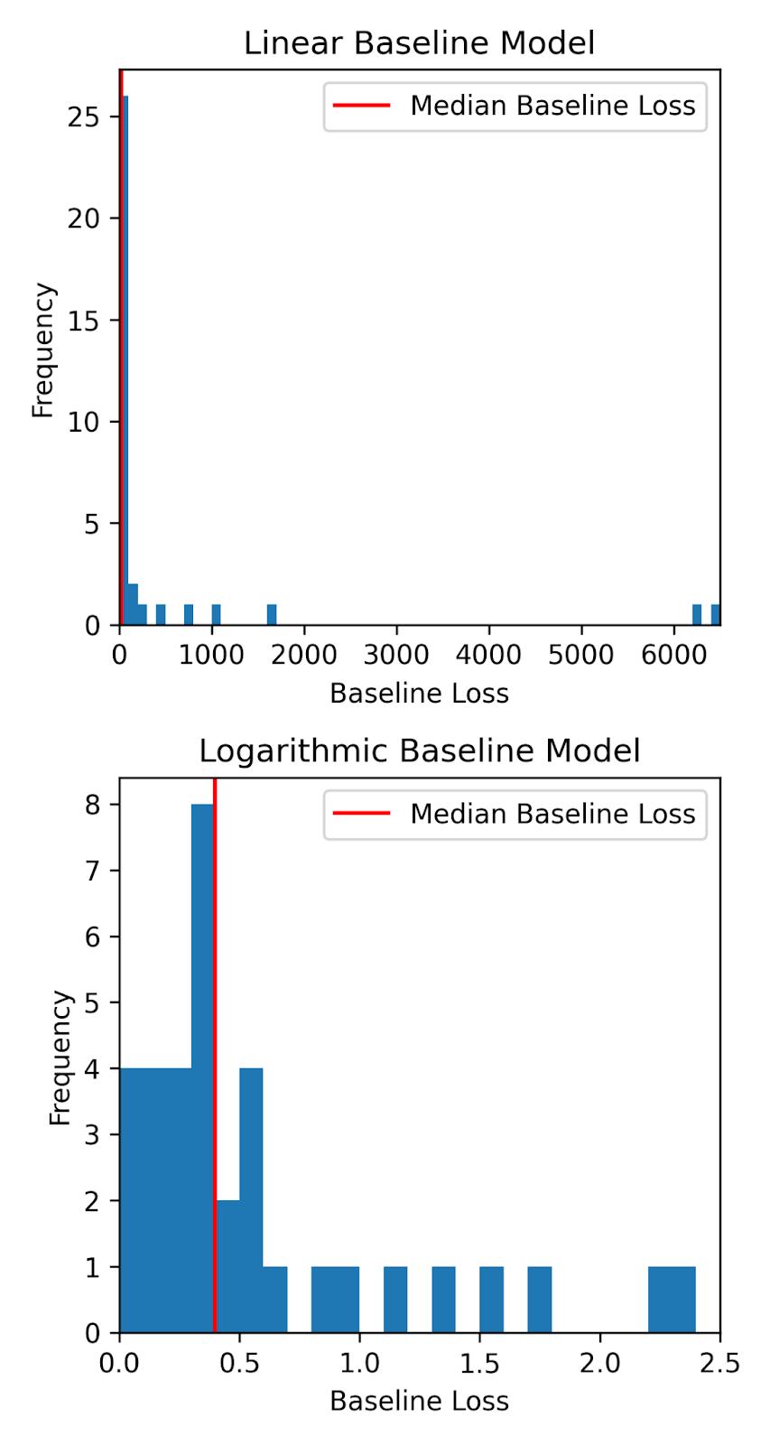
The median baseline loss was 21 for the linear baseline model and 0.40 for the logarithmic baseline model (Figure 6).
Figure 7: Histogram of the error of the predictions of the maximum proton flux made by the linear (top) and logarithmic (bottom) neural network. A negative error indicates that the neural network underestimated the actual value, and a positive error indicates that the neural network overestimated the actual value. The green area corresponds to the region where the neural network’s predictions are more accurate than the corresponding baseline model.
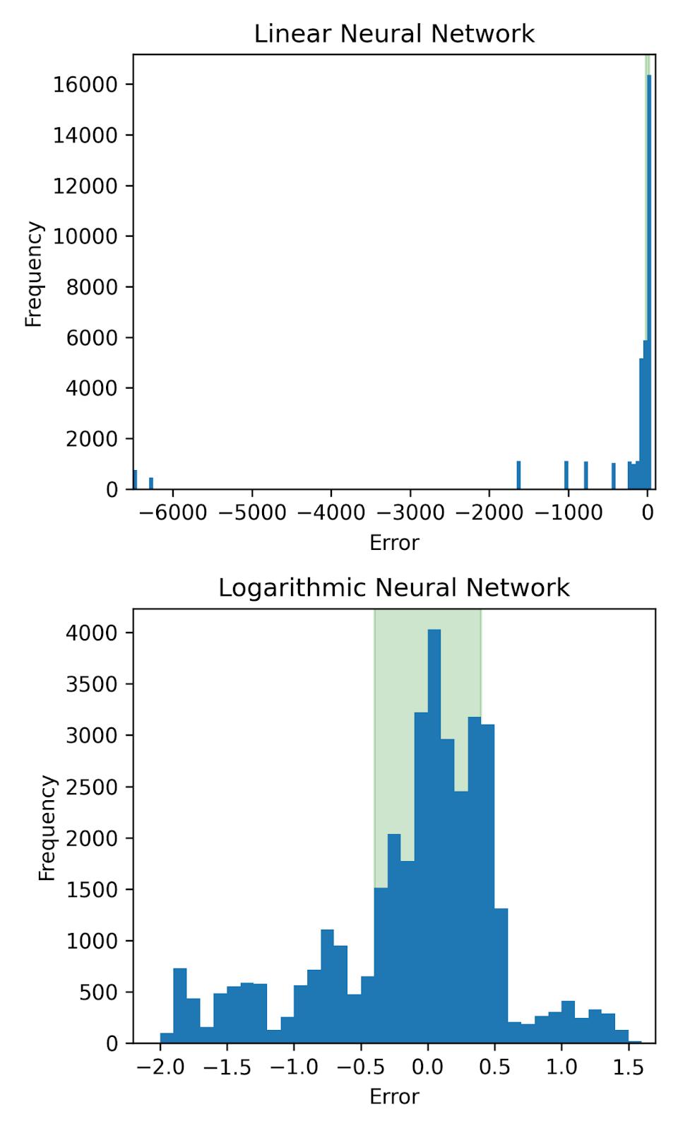
The Journal of Science Extension Research – Vol. 2, 2023 education.nsw.edu.au 248
Figure 8: Histogram of the error of the linear neural network’s predictions of the maximum proton flux caused by actual S1 (minor) SPEs (top), actual S2 (moderate) SPEs (centre), and actual S3 (strong) SPEs (bottom). A negative error indicates that the linear neural network underestimated the actual value, and a positive error indicates that the linear neural network overestimated the actual value. The green area corresponds to the region where the predictions are more accurate than the linear baseline model.
Figure 9: Histogram of the error of the logarithmic neural network’s predictions of the maximum proton flux caused by actual S1 (minor) SPEs (top), actual S2 (moderate) SPEs (centre), and actual S3 (strong) SPEs (bottom). A negative error indicates that the logarithmic neural network underestimated the actual value, and a positive error indicates that the logarithmic neural network overestimated the actual value. The green area corresponds to the region where the predictions are more accurate than the logarithmic baseline model.
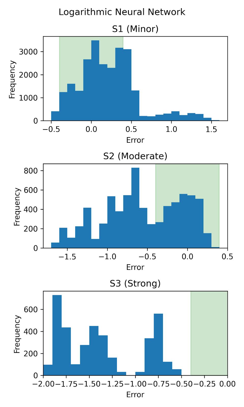
The Journal of Science Extension Research – Vol. 2, 2023 education.nsw.edu.au 249
Figure 10: (Top) Plot of the target values of maximum proton flux against the predictions made by the linear neural network. (Bottom) Plot of the target values of log10(maximum proton flux) against the predictions made by the logarithmic neural network. For both plots, values closer to the line are more accurate, because the line represents an equality between the predicted and target values.
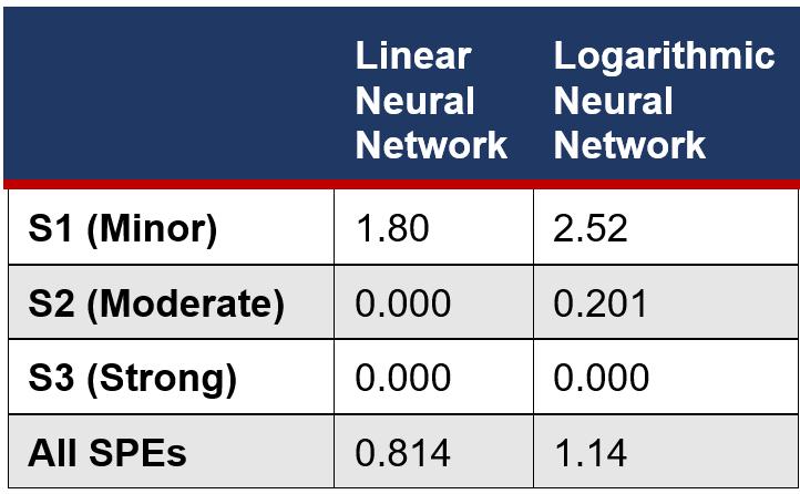
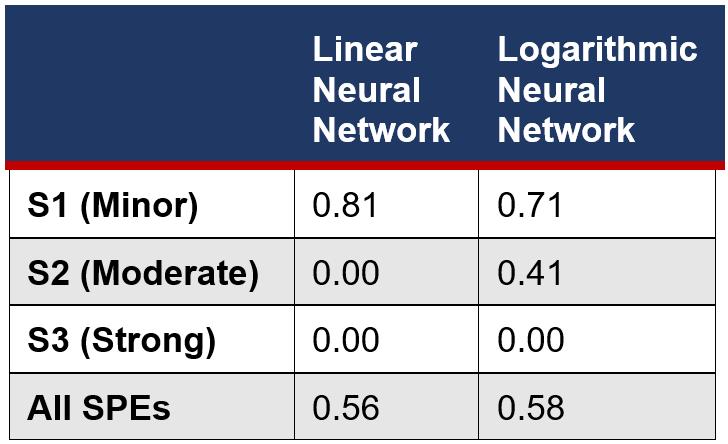
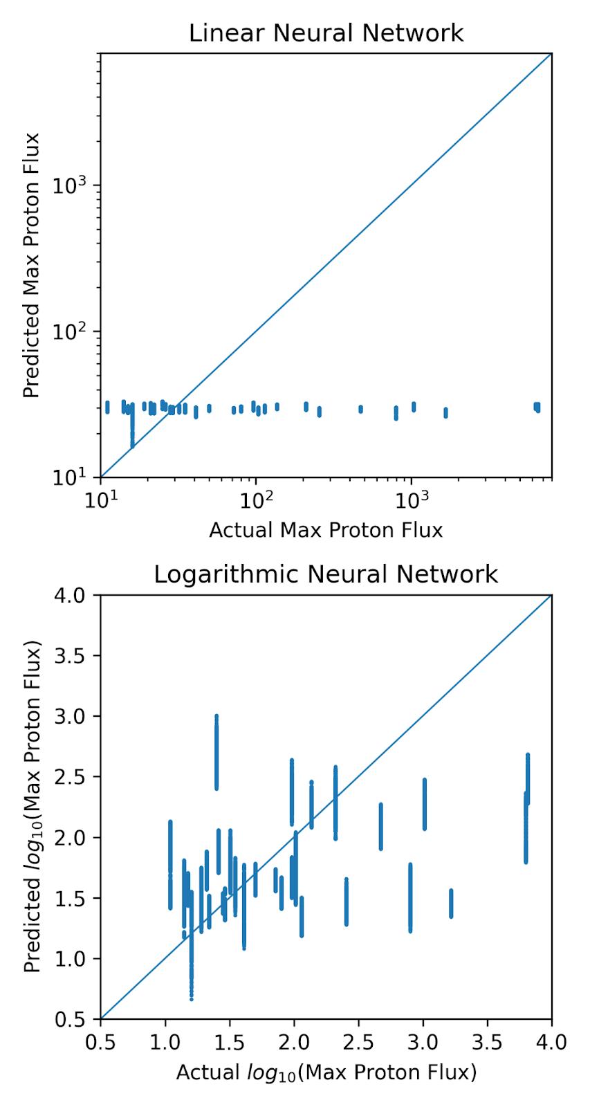
Table 1: Proportion of predictions with error less than the median baseline loss of the corresponding baseline model, p (Equation 2), reported for the predictions of each class of SPE. All values have been reported to two decimal places.
Table 2: Ratio of predictions that overestimated the maximum proton flux to predictions that underestimated the maximum proton flux, η (Equation 3), reported for the predictions of each class of SPE. Values greater than 1 indicate that overestimations were more common than underestimations, and values less than 1 indicate that underestimations were more common than overestimations. All values have been reported to three significant figures.
The Journal of Science Extension Research – Vol. 2, 2023 education.nsw.edu.au 250
Table 3: Sample variance of the target values inputted into, and the predicted values outputted from the linear and logarithmic neural networks. All values have been reported to three significant figures.
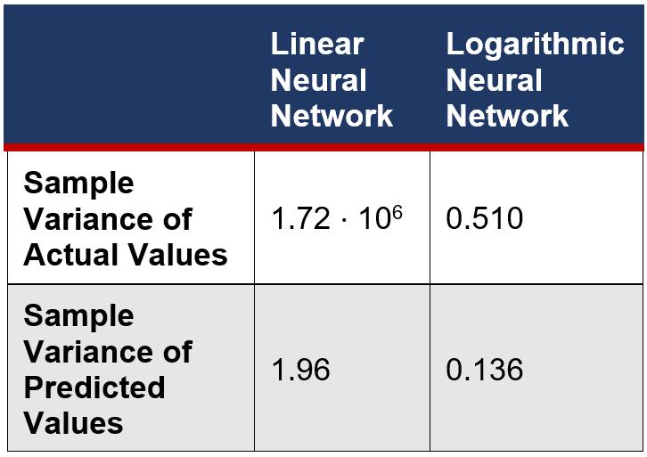
Discussion
A neural network’s performance is quantified by its training and validation loss, the error of its predictions made using the data samples for training and validation respectively. Generally, the training and validation loss decrease as a neural network is compiled for more epochs, however, the validation loss will reach a minimum value where the neural network has been compiled for the optimal number of epochs. After this point, the neural network will overfit to the training data, meaning that it has become too specific to the training data to make accurate predictions using other input data (Figure 11). This trend was observed for the logarithmic neural network, which performed optimally when compiled for 8 epochs (Figure 5). Whilst the training loss for the linear neural network decreased as the epoch number increased, the validation loss did not decrease to a minimum value (Figure 5). It is unlikely that the linear neural network overfitted from the first epoch because this was not observed for the logarithmic neural
network which was trained with the same volume of data. Instead, since the error of the predictions (especially the linear neural network) was negatively skewed (Figure 7), it is likely that the loss function chosen (mean average error) was not appropriate for quantifying the accuracy of the neural network (Pernot et al. 2020).
Figure 11: Typical learning curve for a neural network. The validation (blue) and training (orange) loss are plotted against the epoch number, and the optimal number of epochs is indicated by the dotted line. Figure is adapted from Vogl (2018).
Stronger SPEs, which cause higher maximum proton fluxes at Earth, occur less frequently than weaker SPEs, which cause lower maximum proton fluxes at Earth, because they are produced by rarer, more energetic solar eruptions. Additionally, solar activity varies according to solar cycles which have a periodicity of 11 years, and most SPEs used in this study occurred during Solar Cycle 24 (2008-2019), which was the weakest cycle of the past century (Nandy 2021). Therefore, the distribution of the maximum proton flux of the 35 SPEs in the database of events was positively skewed (Figure 4). This explains why the neural networks were more accurate when predicting weaker SPEs, with both neural networks predicting most S1 (minor) SPEs but no S3 (strong) SPEs with better accuracy than the baseline
The Journal of Science Extension Research – Vol. 2, 2023 education.nsw.edu.au 251
model, which simulated a model with no skill (Table 1). The lack of data for stronger SPEs also accounts for how the neural networks tended to underestimate the maximum proton flux for S2 (moderate) and S3 (strong) SPEs (Figures 7-9, Table 2). Additionally, the variance of the predicted maximum proton flux values was far less than the variance of the target values (Figure 10, Table 3), especially for the linear neural network, implying that the neural networks were unable to differentiate between stronger and weaker SPEs. Therefore, as the neural networks are intended to predict the impact of a SPE on Earth, neither would be useful in a real-life scenario because they would consistently underestimate the magnitude of stronger SPEs. Consequently, authorities would be unable to implement measures to mitigate the greater impact of these stronger SPEs on technologies and humans.
Clearly, the neural networks created in this study require more training data to accurately predict the maximum proton flux corresponding to an SPE. As SPEs rarely impact the Earth, with only 42 events recorded by NASA/NOAA since 2010, it is not feasible to wait until there is a sufficient volume of data to train and validate a neural network which can accurately predict SPEs. Additional vector magnetic data could be sourced using the Spaceweather MDI Active Region Patches (SMARPs) which is a data time series containing three of the SHARP physical parameters with a larger, 96minute cadence for the period January 1996 to October 2010. The SMARP data is derived from the line-of-sight magnetograms taken by the Michelson Doppler Imager (MDI) (Bobra et al. 2021b). Furthermore, additional SPEs
could be sourced using the Space Weather Database Of Notifications, Knowledge, Information (DONKI), which includes SPEs detected by the Solar and Heliospheric Observatory (SOHO) and the Solar Terrestrial Relations Observatory (STEREO) in addition to those detected by the Geostationary Operational Environmental Satellites (GOES) that were used in this study. However, SOHO and STEREO do not orbit the Earth (Figure 12), so SPEs detected by these satellites may not be valid for creating a neural network designed to predict the proton flux at Earth. Alternatively, the neural network could be enhanced using an error penalisation method in which errors when making predictions for SPEs with higher maximum proton fluxes are weighted more than for SPEs with lower maximum proton fluxes, which are overrepresented in the data used in this study (Aminalragia-Giamani et al. 2021).
The Journal of Science Extension Research – Vol. 2, 2023 education.nsw.edu.au 252
Figure
orbit the Sun along the Earth’s orbit path, with STEREO-A (labelled “Ahead”) orbiting ahead of the Earth and STEREO-B (labelled “Behind”) orbiting behind the Earth. SOHO is located at Lagrange Point L1, which lies 1.6 million kilometres towards the Sun from Earth, and orbits the Sun with the same orbital period as Earth. Figure is reproduced from de Sadeleer (2013).
Conclusion
This study investigated the use of vector magnetic data to predict the maximum proton flux experienced at Earth due to an SPE. The SHARP physical parameters describing the magnetic structure in each of the Sun’s ARs were collected for the 24 hours prior to each SPE in the NASA/NOAA Solar Energetic Proton List and collated into data samples which were paired with their corresponding target maximum proton flux values. This dataset was used to train and validate a linear and logarithmic neural network, in which the target values were linearly and logarithmically scaled respectively, using a modified leave-one-
out methodology where the neural networks were trained using the data from all but one of the SPEs, and validated using the data from the remaining SPE. The linear and logarithmic neural networks were benchmarked against the linear and logarithmic baseline models which predicted the maximum proton flux value with no skill.
The accuracies of the linear and logarithmic neural networks were maximised when they were compiled for 1 and 8 epochs respectively. Whilst the neural networks could predict the maximum proton flux for weaker SPEs (e.g. S1 (minor)) more accurately than the corresponding baseline models most of the time, they failed to generate accurate predictions for stronger events (e.g. S3 (strong)). Both neural networks generally underestimated the maximum proton flux caused by SPEs. In conclusion, neither neural network would be accurate enough to be used in a real-life scenario to alert authorities to a strong SPE likely to impact technologies and humans.
References
Abduallah, Y, Jordanova, VK, Liu, H, Li, Q, Wang, JTL & Wang, H 2022, ‘Predicting Solar Energetic Particles
Using SDO/HMI Vector Magnetic Data Products and a Bidirectional LSTM Network’, The Astrophysical Journal Supplement Series, vol. 260, no. 1, viewed 15 May 2022, DOI 10.3847/15384365/ac5f56.
Aminalragia-Giamini, S, Raptis, S, Anastasiadis, A, Tsigkanos, A, Sandberg, I, Papaioannou, A, Papadimitriou, C, Jiggens, P, Aran, A & Daglis, I 2021, ‘Solar Energetic Particle Event occurrence prediction using Solar Flare
12: Positions of the Solar and Heliospheric Observatory (SOHO) and both Solar Terrestrial Relations Observatory (STEREO) spacecraft relative to Earth. The two STEREO spacecraft
The Journal of Science Extension Research – Vol. 2, 2023 education.nsw.edu.au 253
Soft X-ray measurements and Machine Learning’, Journal of Space Weather and Space Climate, vol. 11, viewed 7 February 2022, DOI
10.1051/swsc/2021043.
Anastasiadis, A, Lario, D, Papaioannou, A, Kouloumvakos, A & Vourlidas, A 2019, ‘Solar energetic particles in the inner heliosphere: status and open questions’, Philosophical Transactions of the Royal Society A: Mathematical, Physical and Engineering Sciences, vol. 377, viewed 7 February 2022, DOI
10.1098/rsta.2018.0100.
Bobra, MG, Sun, X, Hoeksema, JT, Turmon, M, Liu, Y, Hayashi, K, Barnes, G & Leka, KD 2014, ‘The Helioseismic and Magnetic Imager (HMI) Vector Magnetic Field Pipeline: SHARPs - Space-Weather
HMI Active Region Patches’, Solar Physics, vol. 289, no. 9, pp. 3549–3578, viewed 27 March 2022, DOI
10.1007/s11207-014-0529-3.
Bobra, MG, Sun, X & Turmon, MJ 2021a, mbobra/SHARPs: SHARPs 0.1.0 (202107-23), Zenodo, viewed 18 June 2022, DOI 10.5281/zenodo.5131292.
Bobra, MG, Wright, PJ, Sun, X & Turmon, MJ 2021b, ‘SMARPs and SHARPs: Two Solar Cycles of Active Region Data’, The Astrophysical Journal Supplement Series, vol. 256, no. 2, viewed 27 March 2022, DOI 10.3847/1538-4365/ac1f1d.
Boucheron, LE, Al-Ghraibah, A & McAteer, RTJ 2015, ‘Prediction of Solar Flare Size and Time-to-Flare Using Support Vector Machine Regression’, Astrophysical Journal, vol. 812, no. 1, viewed 15 July 2022, DOI 10.1088/0004637X/812/1/51.
Chen, Y, Manchester, WB, Hero, AO, Toth, G, DuFumier, B, Zhou, T, Wang, X, Zhu, H, Sun, Z & Gombosi, TI 2019, ‘Identifying Solar Flare Precursors Using Time Series of SDO/HMI Images and SHARP Parameters’, Space Weather, vol. 17, no. 10, pp. 1404–1426, viewed 15 July 2022, DOI 10.1029/2019SW002214.
Chollet, F 2018, Deep Learning with Python, Manning Publications Co., Shelter Island, NY, viewed 16 May 2022, https://tanthiamhuat.files.wordpress.com/ 2018/03/deeplearningwithpython.pdf
de Sadeleer, A 2013, ‘Power, Progress & Prestige: International Relations in Outer Space. A Study in Global Astropolitics, 1940s - 2030s’, Master’s thesis, Université catholique de Louvain, viewed 24 August 2022, https://www.researchgate.net/publication/ 315800396_Power_Progress_Prestige_In ternational_Relations_in_Outer_Space_A _Study_in_Global_Astropolitics_1940s__2030s
Kahler, SW & Ling, AG 2018, ‘Forecasting Solar Energetic Particle (SEP) events with Flare X-ray peak ratios’, Journal of Space Weather and Space Climate, vol. 8, viewed 11 April 2022, DOI 10.1051/swsc/2018033.
Laurenza, M, Alberti, T & Cliver, EW 2018, ‘A Short-term ESPERTA-based Forecast Tool for Moderate-to-extreme Solar Proton Events’, The Astrophysical Journal, vol. 857, no. 2, viewed 8 February 2022, DOI 10.3847/15384357/aab712.
Liu, C, Deng, N, Wang, JTL & Wang, H 2017, ‘Predicting Solar Flares Using SDO /HMI Vector Magnetic Data Products and the Random Forest Algorithm’, The Astrophysical Journal, vol. 843, no. 2,
The Journal of Science Extension Research – Vol. 2, 2023 education.nsw.edu.au 254
viewed 15 May 2022, DOI 10.3847/15384357/aa789b.
Liu, H, Liu, C, Wang, JTL & Wang, H 2019, ‘Predicting Solar Flares Using a Long Short-term Memory Network’, The Astrophysical Journal, vol. 877, no. 2, viewed 15 May 2022, DOI 10.3847/15384357/ab1b3c.
Liu, H, Liu, C, Wang, JTL & Wang, H 2020, ‘Predicting Coronal Mass Ejections Using SDO/HMI Vector Magnetic Data Products and Recurrent Neural Networks’, The Astrophysical Journal, vol. 890, no. 1, viewed 15 May 2022, DOI 10.3847/1538-4357/ab6850.
Murray, SA 2018, ‘The Importance of Ensemble Techniques for Operational Space Weather Forecasting’, Space Weather, vol. 16, no. 7, pp. 777–783, viewed 5 February 2022, DOI 10.1029/2018SW001861.
Nandy, D 2021, ‘Progress in Solar Cycle Predictions: Sunspot Cycles 24-25 in Perspective’, Solar Physics, vol. 296, no. 3, viewed 12 August 2022, DOI 10.1007/s11207-021-01797-2.
National Oceanic and Atmospheric Administration n.d., NOAA Space Weather Scales, viewed 31 July 2022, https://www.swpc.noaa.gov/noaa-scalesexplanation
National Oceanic and Atmospheric Administration 2022, Solar Proton Events Affecting the Earth Environment, viewed 12 August 2022, ftp://ftp.swpc.noaa.gov/pub/indices/SPE.t
of solar EUVs and energetic protons’, Journal of Space Weather and Space Climate, vol. 9, viewed 7 February 2022, DOI 10.1051/swsc/2019025.
Núñez, M & Paul-Pena, D 2020, ‘Predicting >10 MeV SEP Events from Solar Flare and Radio Burst Data’, Universe, vol. 6, no. 10, viewed 7 February 2022, DOI
10.3390/universe6100161.
Papaioannou, A, Sandberg, I, Anastasiadis, A, Kouloumvakos, A, Georgoulis, MK, Tziotziou, K, Tsiropoula, G, Jiggens, P & Hilgers, A 2016, ‘Solar flares, coronal mass ejections and solar energetic particle event characteristics’, Journal of Space Weather and Space Climate, vol. 6, viewed 29 March 2022, DOI 10.1051/swsc/2016035.
Papaioannou, A, Anastasiadis, A, Kouloumvakos, A, Paassilta, M, Vainio, R, Valtonen, E, Belov, A, Eroshenko, E, Abunina, M & Abunin, A 2018, ‘Nowcasting Solar Energetic Particle Events Using Principal Component Analysis’, Solar Physics, vol. 293, no. 7, viewed 16 February 2022, DOI 10.1007/s11207-018-1320-7.
Pernot, P, Huang, B & Savin, A 2020, ‘Impact of non-normal error distributions on the benchmarking and ranking of quantum machine learning models’, Machine Learning: Science and Technology, vol. 2, no. 1, viewed 10 August 2022, DOI 10.1088/26322153/abc350.
Núñez, M, Nieves-Chinchilla, T & Pulkkinen, A 2019, ‘Predicting wellconnected SEP events from observations
Pulkkinen, T 2007, ‘Space Weather: Terrestrial Perspective’, Living Reviews in Solar Physics, vol. 4, viewed 1 February 2022, DOI 10.12942/lrsp-2007-1.
xt
The Journal of Science Extension Research – Vol. 2, 2023 education.nsw.edu.au 255
Schwenn, R 2006, ‘Space Weather: The Solar Perspective’, Living Reviews in Solar Physics, vol. 3, viewed 1 February 2022, DOI 10.12942/lrsp-2006-2.
Stumpo, M, Benella, S, Laurenza, M, Alberti, T, Consolini, G & Marcucci, M 2021, ‘Open Issues in Statistical Forecasting of Solar Proton Events: A Machine Learning Perspective’, Space Weather, vol. 19, no. 10, viewed 8 February 2022, DOI
10.1029/2021SW002794.
Vlahos, L, Anastasiadis, A, Papaioannou, A, Kouloumvakos, A, & Isliker, H 2019, ‘Sources of solar energetic particles’, Philosophical Transactions of the Royal Society A: Mathematical, Physical and Engineering Sciences, vol. 377, viewed 9 February 2022, DOI
10.1098/rsta.2018.0095.
Vogl, R 2018, ‘Deep Learning Methods for Drum Transcription and Drum Pattern Generation’, PhD thesis, Johannes Kepler University Linz, viewed 24 August 2022, DOI
10.13140/RG.2.2.34638.51529.
Wang, J, Liu, S, Ao, X, Zhang, Y, Wang, T & Liu, Y 2019, ‘Parameters Derived from the SDO/HMI Vector Magnetic Field Data: Potential to Improve Machinelearning-based Solar Flare Prediction Models’, The Astrophysical Journal, vol. 884, no. 2, viewed 19 February 2022, DOI 10.3847/1538-4357/ab441b.
Zhong, Q, Wang, J, Meng, X, Liu, S & Gong, J 2019, ‘Prediction Model for Solar Energetic Proton Events: Analysis and Verification’, Space Weather, vol. 17, no. 5, viewed 27 March 2022, DOI
10.1029/2018SW001915.
The Journal of Science Extension Research – Vol. 2, 2023 education.nsw.edu.au 256
Analysis of Properties of Transition Disk Post-AGB Binary Systems for Planet Formation
Yi Wei Yang
James Ruse Agricultural High School
Post-Asymptotic Giant Branch binaries are surrounded by large disks of dust and gas that exhibit conditions reminiscent of young protoplanetary systems conducive to planet formation. This work aims to analyse if properties such as chemical abundances of the post-AGB star may correlate with planet occurrence established by previous photometric analysis. The spectroscopic data for the sample of all known Galactic transition disk postAGB binaries was assembled by mining various abundance studies. Cross-correlation analysis for stars categorised to contain planets was undertaken, and compared to the patterns and signatures of planet-containing stars within the Kepler survey. Planetcontaining galactic post-AGB binaries were found to exhibit higher median elemental abundances but lower metallicities ([Fe/H]) than the population, contrasting with the wellestablished Planet-Metallicity Correlation - where higher metallicities correlated with planet formation. Furthermore, elevated abundances of elements such as carbon, silicon, sulfur, and manganese has also been observed within the planet-containing sample.
1. LITERATURE REVIEW
1.1. Background & Motivations
Understanding planet formation and the role of chemical elements within this process is an integral aspect of astronomy, providing insight into the evolution of our universe. This study will analyse all properties, such as the temperature, metallicity, and chemical abundance, of the post-AGB binary stars in the galactic sample presented by Kluska et al. (2022) to understand planet formation within these systems. This study will not only consider the post-AGB binary sample as a whole, but will also give special focus to each category of disk type to identify similarities and
differences within the sample to find potential chemical and physical anomalies.
1.1.1. Stellar Evolution
Stars are born in areas of particularly dense gravitationally collapsing clouds of dust and gas (nebulae) 1, beginning their lives on the Main Sequence (see Figure 1), fusing hydrogen into helium as the dominant energy production process. The collapse of this cloud of dust and gas will also result in the formation of an accretion disk 2 around the protostar, with further gravitational accumulation and accretion of particles within the disk leading to 1stgeneration planet formation.
1 which are largely composed of molecular hydrogen within a very sparse interstellar medium (10
4 to 106 particles per cm3)
2 composed of leftover material from the initial gravitational collapse
The Journal of Science Extension Research – Vol. 2, 2023 education.nsw.edu.au 257
The composition and mass of the protostellar material will greatly affect the life-cycle of the resultant star. Generally, for a 1 M⊙ (one solar mass) star, as it consumes most of the hydrogen within its core, it will expand and cool, evolving into a red giant as it fuses heavier elements such as helium for energy production; this is characterised by the Red Giant Branch (RGB) of the H-R diagram in Figure 1. As the star continues to consume its fusion products, its temperature and luminosity evolves within this region, cooling and expanding. Near the end of this giant branch evolution is the Asymptotic Giant Branch (AGB), where the star expands to several hundred times it previous volume and generates approximately half of the elements heavier than iron (e.g.
zirconium, barium, cerium, lead) via the slow-neutron capture process (sprocess). As the star approaches the end of the AGB phase, it will shed its cooler outer layer, exposing the chemically enriched surface of the star; this is known as the post-AGB phase (van Winckel 2003; Kamath 2020). The post-AGB star will continuously increase in temperature, ionising its ejected outer layers of gas to form a planetary nebula (PN), expelling the heavy elements produced by nucleosynthesis back into the interstellar medium (Sloan et al. 2008). Finally, as the PN cools, what remains is an extremely dense stellar remnant (a white dwarf) that will continue to cool for billions of years to come.
Figure
evolutionary track of a Sunlike star. The diagram plots a star’s luminosity against its surface temperature and is an extremely useful tool in astronomy to characterise a star’s properties. Note that neither time nor position in space is an axis within this diagram, so as a star evolves along an evolutionary track, it is not physically travelling anywhere, nor is the rate at which it is progressing along the track constant. Credit: Adapted from Pearson Education 2004
1.1.2.
Evolutionary theory predicts that lowintermediate mass (0.6 M⊙ to 8 M⊙) post-
AGB stars form in the transition between the AGB and a PN phases (see Figure 1). They appear as very luminous red giant stars with unique characteristics, having ejected their outer layers to reveal the
 1. Hertzsprung-Russell diagram (H-R diagram) with an
Post-Asymptotic Giant Branch Stars
1. Hertzsprung-Russell diagram (H-R diagram) with an
Post-Asymptotic Giant Branch Stars
The Journal of Science Extension Research – Vol. 2, 2023 education.nsw.edu.au 258
star’s inner core for an astronomically short time period of 103 − 104 years 3 (van Winckel 2003). This inner core is composed of largely inert carbon and oxygen enriched with heavy elements formed from the s-process nucleosynthesis reactions. They exhibit a unique Spectral Energy Distribution (SED) which is characterised by two distinct curves, one in the shorter wavelengths generated by the inner star itself and the curve in the longer wavelengths due to the cooler shell of dust surrounding the star.
1.1.3. Binary Post-Asymptotic Giant Branch Stars
In a binary system, as one of the stars evolves and expands, material from one star can spill towards its partner, forming an accretion disk, also termed a transition disk 4 (Strom et al. 1989; Calvet et al. 2002, 2005; Kluska et al. 2022). These transition disks exhibit very similar properties to the protoplanetary disk around young stars(de Ruyter et al. 2006) described in Section 1.1.2, displaying potential to form second generation planets (Ertel et al. 2019). Post-AGB stars in a binary system (with a main sequence partner) also exhibit a characteristic depletion of refractory elements 5, not due to nucleosynthetic processes (Maas et al. 2003; Oomen et al. 2019), but rather, due to the rapid early condensation of these refractory elements as the post-AGB star expels its outer gaseous shells into the dusty disks, which are then blown away by radiation
pressure whilst the volatile gaseous elements remain to be re-accreted into the post-AGB star.
In the spectral energy distribution (Figure 3), two blackbody curves are also similarly present 6 compared to the single post-AGB SED. However, this secondary curve is noticeably different from that of a single post-AGB star, appearing as a less distinct infrared excess.
Figure 2. Adapted from van Aarle et al. (2011). The spectral energy distribution for HD 56126, a carbon-rich single postAGB star, in the infrared region. The black curve represents the core star and the red curve represents the secondary blackbody spectrum due to the ejected dust shell.
3 comparatively, main sequence stars like the Sun can survive for 106 − 109 years
4 as they can be thought to be transitioning between full dusty disks and gas-less debris disks
5 elements that have relatively higher condensation temperatures, such as titanium
6 a curve within the shorter wavelengths is the core star’s blackbody distribution, and a curve in the longer wavelengths represents the scattering of light in the dusty transition disk, again shifted due to the dust’s temperature being cooler than the star itself.
The Journal of Science Extension Research – Vol. 2, 2023 education.nsw.edu.au 259
Figure 3. Adapted from Kluska et al. (2022). The spectral energy distribution for IRAS19291+2149, a post-AGB binary, in the infrared region. The red is the best fit photospheric model for the core star, and the blue represents the Spitzer spectrum, highlighting the secondary blackbody spectrum due to the transition disk.
1.1.4. Target Sample
Binary post-AGB stars are potential sites of second generation planet formation so the sample from Kluska et al. (2022) was chosen as our target. This sample contains a list of all galactic post-AGB binaries characterised by their photometric properties by comparing the intensities of different wavelengths of emitted light (photometric bands) to identify larger scale properties such as stellar temperature, and disk structures by comparing the two unique blackbody curves within the SED (e.g. Figure 3);
these disk structures within each category is displayed in Figure 4.
The Two Micron All-Sky Survey (2MASS) provided photometry in the near-IR wavelengths (conducted by various ground-based observatories) (Skrutskie et al. 2006), and the WISE surveys (conducted by the Wide-field Infrared Survey Explorer spacecraft) (Wright et al. 2010) provided mid- to far-infrared photometric data. Extremely highresolution spectra to provide chemical and kinematic information for target stars were generated by the APOGEE surveys (Apache Point Observatory Galactic Evolution Experiment) (Majewski et al. 2017) that characterised over half a million stars through near-infrared observation by measuring the intensity of certain spectral lines to determine chemical abundance; this is commonly notated as the logarithmic ratio of the desired element and hydrogen or iron compared to the Sun (i.e. [���� /���� ] = ������������10 (�������� /�������� )���������������� ������������10 (�������� /�������� )������������ , where N denotes no. of particles and X denotes the element studied). A notable ratio is [Fe/H], known as metallicity, and is used as a measure of the abundance of elements heavier than helium (note all elements heavier than hydrogen and helium are termed a ‘metal’ within astronomy) 7
The Journal of Science Extension Research – Vol. 2, 2023 education.nsw.edu.au 260
7 Other properties such as temperature and surface gravity are modelled via methods such as the Boltzmann excitation equation and Saha ionisation equation respectively, but is outside of the scope of this work.
1.1.5. Planet Metallicity Correlation
A Planet-Metallicity Correlation (PMC) has been found in many spectroscopic surveys, first recognised in exoplanet searches (Gonzalez 1997), which has lead to more detailed, larger scale investigations of this trend, producing a well-established correlation between planetary architecture and metallicity: higher metallicities of the host star correlated with increased planet formation. This is due to how the star’s chemistry is reflective of its homogeneous protostellar environment (Spina et al. 2021) - planets largely accrete from the heavier elements (metals) rather than hydrogen and helium.
Wilson et al. (2022) also expanded this work to the Kepler spectroscopic surveys (the Kepler space telescope targeted most G-type stars on/near the main sequence, see Figure 1) and found that a general increase in elemental abundance (C, Mg, Al, Si, S, K, Ca, Mn, Fe, and Ni) was correlated with an increase in planet occurrence, particularly larger planets with wider orbits. This was accomplished by assembling (from the Kepler survey) a
sample of planet-containing stars and a control sample of stars chosen with properties (e.g. temperature, mass, photometric magnitudes) that reflect the bulk properties of the Kepler survey sample.
2. SCIENTIFIC FOCUS
Data from a variety of surveys (described in Section 1.1.4) is utilised to construct a comprehensive profile of transition disk properties, including the temperature, metallicity, and chemical abundance, of post-AGB binaries to extend a study by Wilson et al. (2022) which identified chemical anomalies in the composition of planet-containing stars from the Kepler survey that targeted younger, main sequence stars.
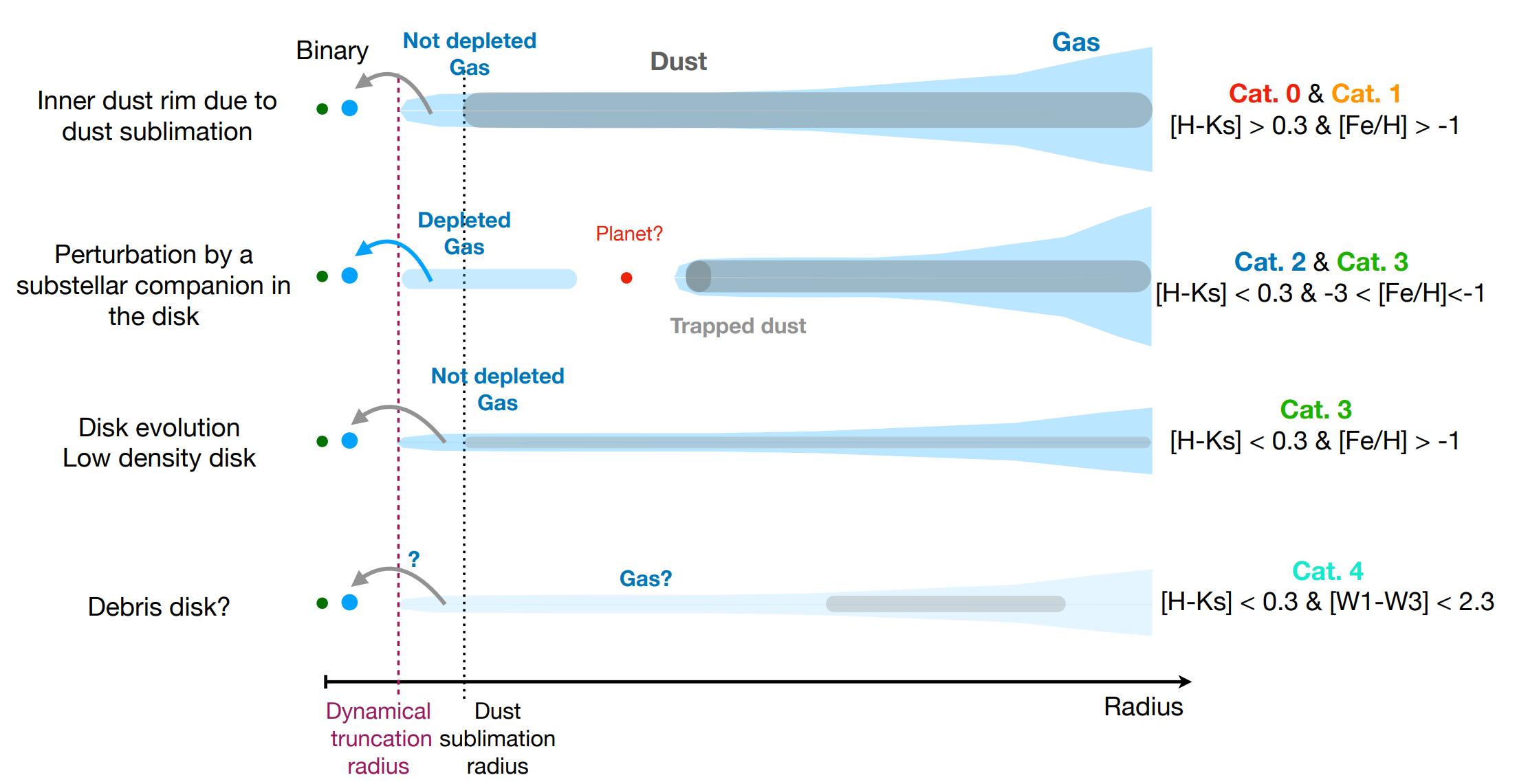
Thus, the scientific research question is: Do planet hosting Post-AGB binaries show trends between stellar properties and second generation planet formation that are valid proxies for planet identification?
3. METHODOLOGY
3.1. Data Collection
Figure 4. Theorised scenarios for each category (Kluska et al. 2022) .
The Journal of Science Extension Research – Vol. 2, 2023 education.nsw.edu.au 261
This study applied data from very recent papers (Kluska et al. 2022; Wilson et al. 2022) to search for planet-containing post-AGB binaries. I attempted to characterise stellar properties through stellar chemistry and other photometric properties by comparing trends found within this paper with the properties characterised by their SEDs by (Kluska et al. 2022). The target sample (Table 1) is a thorough list of post-AGB binaries that exhibit transition disks - the focus of this study. The chemical abundances for the elements studied by Wilson et al. (2022) (C, Mg, Al, Si, S, K, Ca, Mn, Fe, and Ni) expressed as [X/H] or [X/Fe]) were obtained by mining data from relevant abundance studies listed in Kluska et al. (2022). These elements allowed for a more direct cross-correlation comparisons and were also most commonly present within all the abundance studies (i.e. abundance studies did not always provide chemical abundances for every element). The respective temperature models and their stellar abundances models for each star were compiled into a single large spreadsheet. The categorisation by Kluska et al. (2022) was extended to include an additional category, ‘Cat. 3p’, to isolate the planet-containing stars in
Cat. 3. Overall, these categories range from 0 to 4, with Cat. 2 and Cat. 3p’s transition disks exhibiting properties that are indicative of planet presence.
3.1.1. Cleansing
A significant amount of data cleansing was not required as the target sample was very definitive in containing all galactic post-AGB binaries. Stars where abundance values could not be found (i.e. the references did not lead to full abundance studies and no abundance data could be found) were omitted from the sample. This removed 25 stars from the original sample of 85, leaving 60 stars - this should still be noted to be a significant, large sample of post-AGB stars due to their rarity from their extremely short lifespans detailed in Section 1.1.1, so should still generate valid and significant results.
3.2. Data Processing
All abundances were converted to the abundance ratio of [X/Fe] using the formula [X/Fe] = [X/H] + [Fe/H] (noting that [Fe/H] is metallicity, which was one of the attributes collated by Kluska et al. (2022) within his star sample).
The Journal of Science Extension Research – Vol. 2, 2023 education.nsw.edu.au 262
A Python program utilising Matplotlib was developed to produce various plots to process the data for analysis, with a unique marker used to denote each category of transition disk type across all plots:
• Abundance ratio of each element was plotted against effective temperature (stellar surface temperature), with a colourmap applied to show metallicity. Median lines were added, similarly to Wilson et al. (2022), to display potential trends between abundance and temperature which would invalidate trends observed in other graphs as a result of this spurious correlation; ideally, the crosses, representing the medians with bins of 500K, should remain close to the median without any significant correlation. Standard deviation intervals of 0.5σ, 1σ, and 2σ of the entire sample are also represented with grey lines to display the spread of data.
• Metallicity [Fe/H] was plotted against effective temperature. Medians for the planet-containing sample and the entire star sample was also plotted to allow for comparison between the two populations. Standard deviation intervals of 0.5σ, 1σ, and 2σ of the entire sample are also represented with grey lines to display the spread of data.
• Metallicity [Fe/H] was plotted against the orbital period of the
binary system (note: this is not orbital period of potential planets). Medians for the planet-containing sample and the star sample was also plotted to allow for comparison between the two populations. Standard deviation intervals of 0.5σ, 1σ, and 2σ of the entire sample are also represented with grey lines to display the spread of data.
• Abundance ratio of each element was plotted against metallicity [Fe/H] with a linear regression model fitted to the planet-containing sample (green) and to the star sample (black). Standard deviation intervals of 0.5σ, 1σ, and 2σ of the entire sample are also represented with grey lines to display the spread of data.
• Abundance ratio of each element was plotted against metallicity [Fe/H], with the respective planet and control medians of the Kepler sample from Wilson et al. (2022).
This methodology has provided a comprehensive overview of the relationships between many different stellar properties to most effectively display differences within planetcontaining sample. Additionally, negligible risks and safety issues were present in this project due to its digital nature - all astrophysical data was obtainable from online databases and literature.
The Journal of Science Extension Research – Vol. 2, 2023 education.nsw.edu.au 263
4. RESULTS
The graphs and plots outlined within Section 3.2 are displayed in the following figures:
Figure 5. Abundance ratio vs effective temperature with a colourmap of metallicity. The horizontal red dashed lines represents the median of the sample. The solid black vertical and horizontal lines indicate the means of effective temperature and abundance ratio respectively. The white crosses represent the medians of bins of 500K. The grey grid represents standard deviation intervals of 0.5σ, 1σ, and 2σ for each axis.
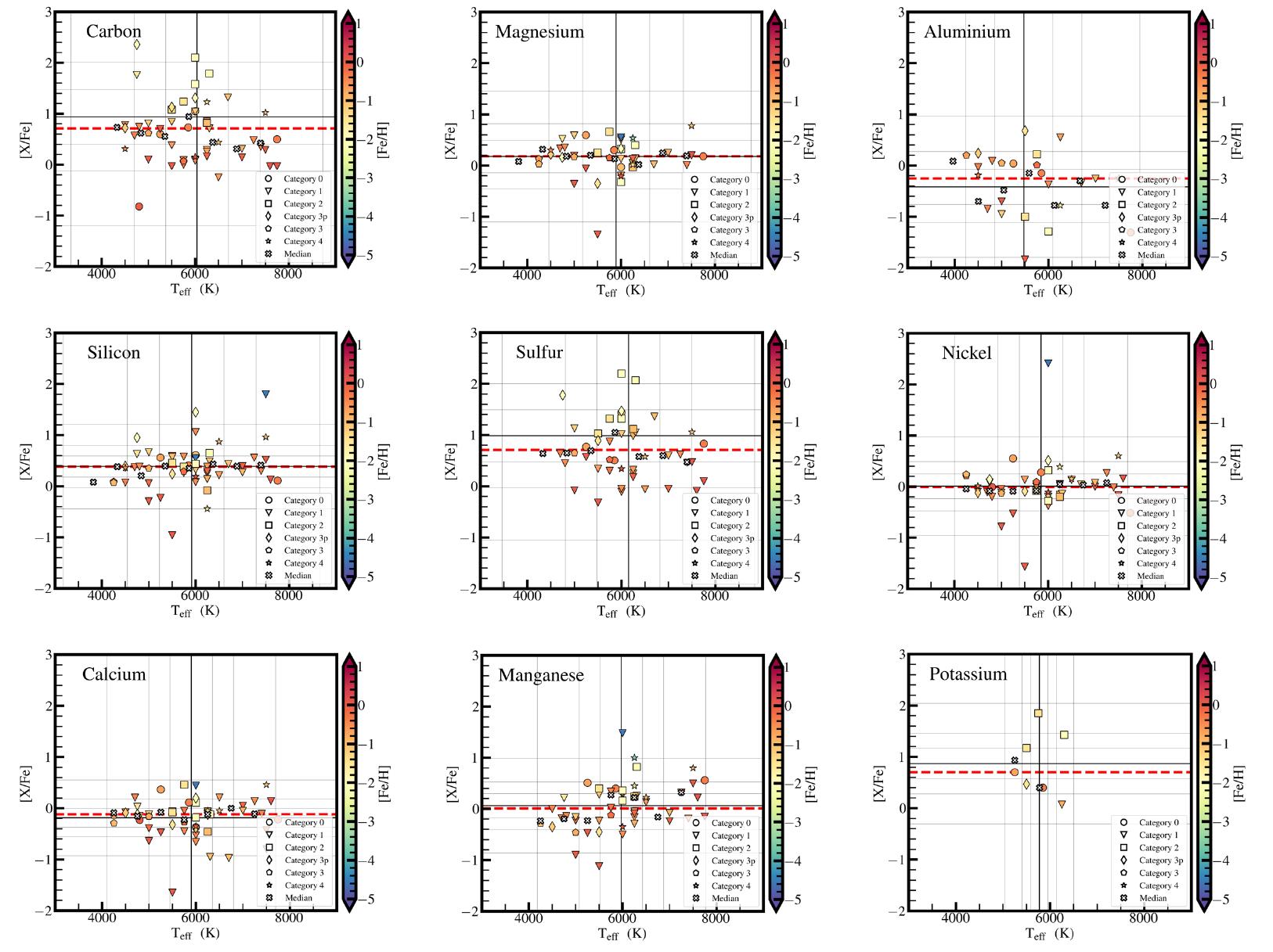
The Journal of Science Extension Research – Vol. 2, 2023 education.nsw.edu.au 264
Figure 6. Metallicity vs effective temperature. Lime represents the planet-containing sample, cyan represents the non-planet-containing sample. The green dashed horizontal line indicates the median of metallicity of the planet-containing sample. The green dashed vertical line represents the median temperature of the planet-containing sample. The black dashed horizontal line indicates the median of metallicity of the entire target sample. The black dashed vertical line represents the median temperature of the entire target sample. The solid black vertical and horizontal lines indicate the means of effective temperature and metallicity respectively of the entire target sample. The grey grid represents standard deviation intervals of 0.5σ, 1σ, and 2σ for each axis.
Figure 7. Metallicity vs orbital period of the binary system. Lime represents the planetcontaining sample, cyan represents the non-planet-containing sample. The green dashed vertical and horizontal lines represents the median values of orbital period and metallicity respectively for the planet-containing sample. The black dashed vertical and horizontal lines represents the median values of orbital period and metallicity respectively of the entire target sample. The solid black vertical and horizontal lines indicate the means of orbital period and metallicity respectively. The grey grid represents standard deviation intervals of 0.5σ, 1σ, and 2σ for each axis.
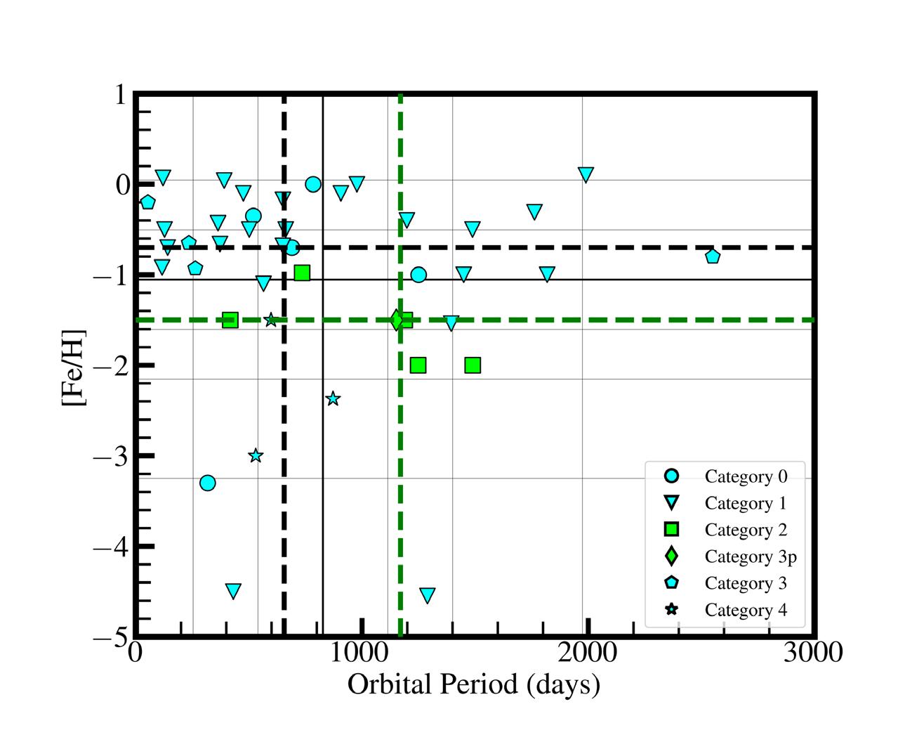
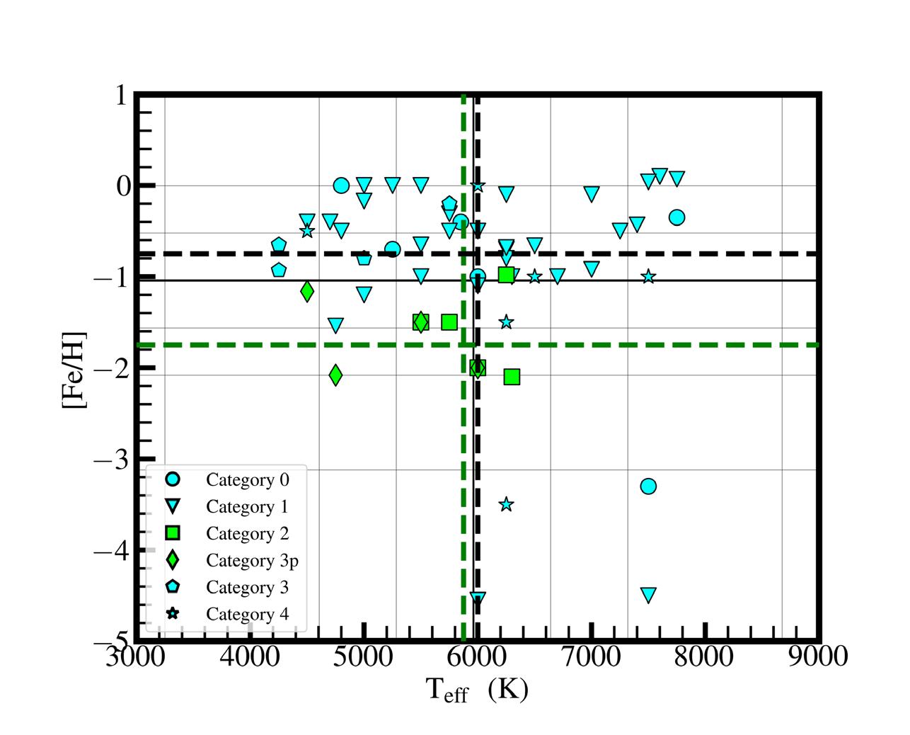
The Journal of Science Extension Research – Vol. 2, 2023 education.nsw.edu.au 265
Figure 8. Plots of abundance vs metallicity. Lime represents the planet-containing sample, cyan represents the non-planet-containing sample. Regression lines are in green and black representing the planet-containing sample and entire target sample respectively. The solid black vertical and horizontal lines indicate the means of metallicity and abundance ratio respectively. The grey grid represents standard deviation intervals of 0.5σ, 1σ, and 2σ for each axis. Note the strongest regression lines for the entire target sample have Pearson’s correlation coefficients and p-values of:
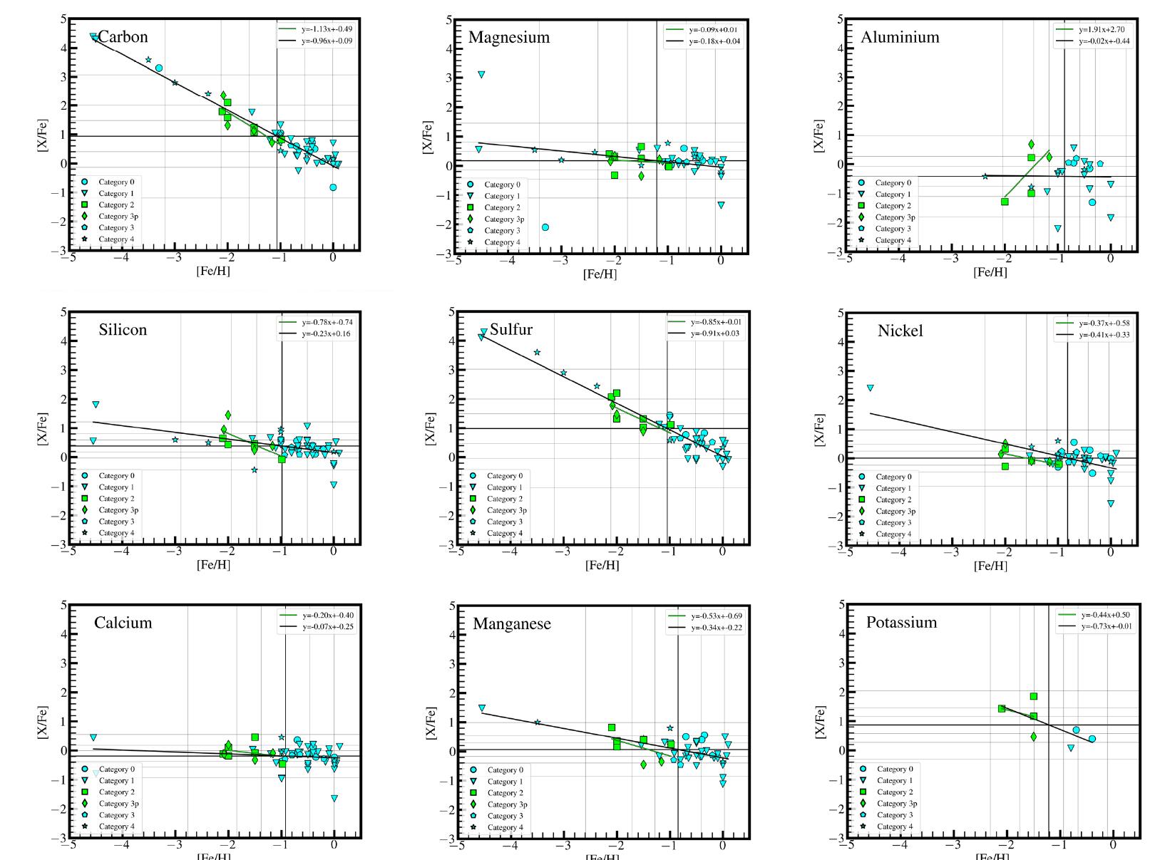
����������������������������
−����. ��������, ���������������������������� = ����. ���� × �������� �������� ; ���������������������������� = −���� ��������, ���������������������������� = ���� ���� × �������� �������� ; �������������������������������� = −���� ��������, �������������������������������� = ���� ���� × �������� ���� ; ���������������������������� = −���� ��������, ���������������������������� = ����. ���� × �������� ���� . The Journal of Science Extension Research – Vol. 2, 2023 education.nsw.edu.au 266
=
Figure 9. Plots of abundance vs metallicity. Lime represents the planet-containing sample, cyan represents the non-planet-containing sample. The green dashed vertical and horizontal lines represent the median values of metallicity and abundance ratio for the planet-containing sample. The black dashed vertical and horizontal lines represent the median values of metallicity and abundance ratio for the star sample. The red and purple dashed lines similarly represent the medians from Wilson et al. (2022) (also see Figure 10); purple is the planet-containing sample, tan is the control sample (refer to Section 1.1.5) .
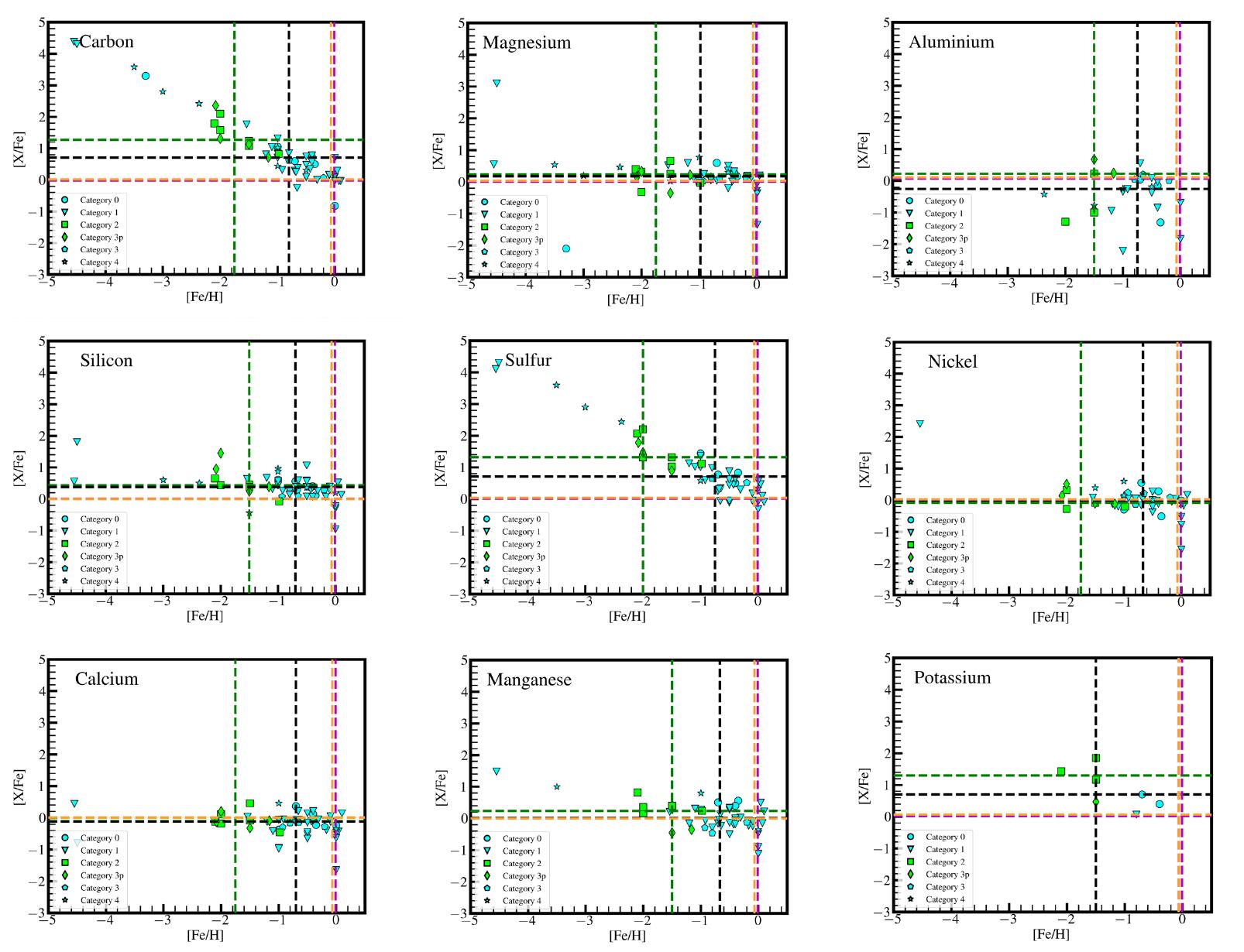
5. DISCUSSION
5.1. Overview
5.1.1. Temperature Relations
Figure 5 displays chemical abundance against temperature with a colourmap displaying metallicity to show potential unwanted trends between temperature and chemical abundance which would lead to spurious correlations within other variables in the following graphs. PostAGB stars can have a large range in temperature depending on their age, so
should not display any particular correlations between these properties:
• The magnesium, silicon, sulfur, nickel, calcium bin medians (the crosses) largely lie very close to this desired range.
• Even though the carbon, aluminum, and manganese bin medians do not all lie close to the desired median range, they effectively display no correlation between chemical abundance and temperature.
• The data sample available for potassium is much smaller than the
The Journal of Science Extension Research – Vol. 2, 2023 education.nsw.edu.au 267
other elements due to a lack of measurement from most abundance analyses (only 7 data points).
Thus, all chemical elements with the exception of potassium are valid for analysis 8; they have sufficiently large sample sizes which display no trends between temperature and chemical abundance. It is also noted that the planet-containing sample (Category 2 and Category 3p) has elevated chemical abundances for the α-elements carbon, silicon, sulfur, manganese, consistently lying above the median, elements that arise from similar nucleosynthetic origins of helium fusion (alpha process).
Within Figure 6, there is little offset in temperature between the medians of the planet-containing and population samples (125K) and the data displays little correlation with a Pearson’s correlation coefficient ���� = 0.14 (note it is slightly skewed by the extreme low metallicity stars, see Section 5.2) which is consistent with Figure 5 and general astronomical literature that no correlation between temperature and chemical properties should be present in post-AGB stars (Wilson et al. 2022).
5.1.2. Orbital Period Relations
An offset to longer stellar orbital periods and lower metallicities is present in the medians of the planet-containing stars compared against the entire sample median is evident within Figure 7, disagreeing with the PMC that higher metallicity stars are more likely to form planets (Osborn & Bayliss 2020). This reveals the need for new planetary
formation models as the PMC only models 1st-generation planet formation; the materials that form 2nd-generation planets within these post-AGB binaries arise from drastically different origins: it is the metal-rich refractory dust expelled by the post-AGB star that forms planets rather than a homogeneous protostellar dust cloud, potentially indicating that planet forming post-AGB stars should be even more depleted in metals as these have left into the disk, which is supported by this data. The exact mechanism behind the offset to longer orbital periods is also unknown, with further researched needed.
5.1.3. Abundance Relations
Strong statistically significant correlations are present in Figure 8 between abundance and metallicity, particularly in the α-elements of carbon, sulfur, and silicon
This result is not present in the Wilson et al. (2022) study of the Kepler stars (see their results in Figure 10, consistent with the aforementioned theory because the younger, main sequence Kepler stars would not have undergone shell ejection processes associated with the post-AGB phase.
Furthermore, despite the slight lack of independence between the variables (i.e. an increase in carbon should result in an increase in metallicity due to the definition of ‘metals’ as elements heavier than helium - and carbon is one such element that is heavier than helium), this
(����������������������������
, ���������������������������� =2.3× 10 31 ; ���������������������������� = 0.95, ���������������������������� =2.6× 10 26 ; �������������������������������� = 0.53, �������������������������������� =2.9× 10⁻⁵ ; ���������������������������� = 0.67, ���������������������������� =1.1× 10⁻⁷ ).
= 0.96
8
for the sake of completeness The Journal of Science Extension Research – Vol. 2, 2023 education.nsw.edu.au 268
the potassium graphs have still been kept, simply
relationship also contradicts this proposition, also indicating further research is required to uncover the exact mechanism behind this trend.
In Figure 9, the medians of the planetcontaining stars are noticeably offset from the sample medians with much lower metallicities, consistent with Figure 7 that 2nd-generation planet formation is associated with extra depleted stars. Additionally, if the extreme depleted stars ([Fe/H] ≤ 3) are disregarded, the planetcontaining stars lie clearly within a separate ‘cluster’ in Figure 9 at much lower metallicities. This offset is not consistent with the results of Wilson et al. (2022), where planet-containing stars have slightly lower metallicities, indicating differences in the process of planet formation that will require further modelling and study.
5.2. Extreme Stars
There are a number of ‘extreme’ stars (HD 52961, HR 4049, CC Lyr, HD 44179, HD 137569) with extremely low metallicities ([Fe/H] ≤ 3). These stars are found to show no obvious links with transition disk formation, suggesting an unknown depletion mechanism is present within the stellar system, and it is unknown if this depletion mechanism is the same as the rest of the target sample population (Kluska et al. 2022). This factor has motivated the use of medians rather than means to provide a more accurate depiction of the data’s central tendency.
5.3. Limitations
Due to the exploratory nature of this study, more information is required on the dust formation and processing within the disks themselves. Current literature does
not fully understand the physics behind the planet formation process within these transition disks such as inhomogeneities within disk material, nor the morphology and true structure of the transitions disks - we only have photospheric parameters from which we attempt to infer properties.
Omitting the stars for which abundance could not be found should not introduce bias, as this was likely due to random chance that the omitted stars did not have accessible chemical abundances. This work has aimed to avoid spurious correlations, such as temperatureabundance relations, but notes many confounding variables that may be present such as relative trends with stellar age, and stellar mass which could not be accounted for due to a lack of data.
5.4. Future Scope
As this project is the first study analysing the chemical composition of different categories of binary post-AGB stars with a special focus on stars with transition disks, significantly more study into the sample is needed, such as developing and comparing these results with stellar models to fully understand the mechanism behind these trends and address the gaps within our knowledge, such as the many peculiar metallicity and abundance relationships. The population of extreme stars also warrants further study into their depletion mechanisms, i.e. what has caused them to become so extremely metal poor.
Another immediate continuation of this work is to extend the sample of analysed post-AGB binaries to increase the statistical significance of results by extending this sample to extra-galactic stars, such as the Magellanic Clouds. In
The Journal of Science Extension Research – Vol. 2, 2023 education.nsw.edu.au 269
addition, explorations on the applicability of the patterns found within this study to other stars, such as single post-AGB systems, can be conducted to produce a more holistic set of parameters defining planet occurrence via stars’ chemical properties.
6. CONCLUSION
This project has characterised how the properties of 2nd-generation planetcontaining post-AGB binaries differ from the galactic population; they have higher orbital periods, and higher median elemental abundances (with particular elevations in the abundances of αelements such as carbon, silicon, sulfur, and manganese) but with lower metallicities. The post-AGB sample disobeys the PMC that characterises 1stgeneration planet forming stars likely due to the very different mechanisms behind disk and planet formation but further research is needed to determine the exact processes involved. The comparison of this study’s results with the Kepler stars in Wilson et al. (2022) have also reflected this theory, where the postAGB sample had much lower metallicities whilst the planet-containing Kepler sample of main sequence stars had higher metallicities that followed the PMC.
ACKNOWLEDGEMENTS
I would like to thank my science extension teacher, Dr Dennis, for her tireless support of this project, by providing constant guidance, putting me in touch with my Macquarie University mentor, Dr Kamath, and help in proofreading and editing this report.
I would also like to thank Dr Kamath and her group of PhD students for teaching me so much about astronomy and post-
AGB stars, and her patience in guiding me until its completion, allowing me to gain the wide range of astrophysical knowledge and skills required for this project, including how to utilise the NASA ADS system to effectively find literature, and the use of LATEX to typeset my report, not to mention her assistance in also proofreading and editing this report to point me in the right direction in this project.
I would also like to extend my thanks to my friends, Michael Chen and Kerui Yang, who have supported me in proofreading my work and helped troubleshoot issues when things went wrong within my Python scripts and project.
REFERENCES
Calvet, N., D’Alessio, P., Hartmann, L., et al. 2002, ApJ, 568, 1008, doi: 10.1086/339061
Calvet, N., D’Alessio, P., Watson, D. M., et al. 2005, ApJL, 630, L185, doi: 10.1086/491652
de Ruyter, S., van Winckel, H., Maas, T., et al. 2006, A&A, 448, 641, doi: 10.1051/0004-6361:20054062
Ertel, S., Kamath, D., Hillen, M., et al. 2019, AJ, 157, 110, doi: 10.3847/15383881/aafe04
Gezer, I., Van Winckel, H., Bozkurt, Z., et al. 2015, MNRAS, 453, 133, doi: 10.1093/mnras/stv1627
Gezer, I., Van Winckel, H., Manick, R., & Kamath, D. 2019, MNRAS, 488, 4033, doi: 10.1093/mnras/stz1967
The Journal of Science Extension Research – Vol. 2, 2023 education.nsw.edu.au 270
Giridhar, S., & Arellano Ferro, A. 2005, A&A, 443, 297, doi: 10.1051/00046361:20041495
Giridhar, S., Molina, R., Arellano Ferro, A., & Selvakumar, G. 2010, MNRAS, 406, 290, doi: 10.1111/j.13652966.2010.16696.x
Gonzalez, G. 1997, MNRAS, 285, 403, doi: 10.1093/mnras/285.2.403
Gorlova, N., Van Winckel, H., Gielen, C., et al. 2012, A&A, 542, A27, doi: 10.1051/0004-6361/201118727
Gorlova, N., Van Winckel, H., Ikonnikova, N.P., et al. 2015, MNRAS, 451, 2462, doi: 10.1093/mnras/stv1111
Kamath, D. 2020, Journal of Astrophysics and Astronomy, 41, 42, doi: 10.1007/s12036-020-09665-4
Klochkova, V. G., & Panchuk, V. E. 1996, Bulletin of the Special Astrophysics Observatory, 41, 5
Kluska, J., Van Winckel, H., Copp´ee, Q., et al. 2022, A&A, 658, A36, doi: 10.1051/0004-6361/202141690
Maas, T., Giridhar, S., & Lambert, D. L. 2007, ApJ, 666, 378, doi: 10.1086/520081
Maas, T., Van Winckel, H., Lloyd Evans, T., et al. 2003, A&A, 405, 271, doi: 10.1051/0004-6361:20030613
Majewski, S. R., Schiavon, R. P., Frinchaboy, P. M., et al. 2017, AJ, 154, 94, doi: 10.3847/1538-3881/aa784d
Manick, R., Miszalski, B., Kamath, D., et al. 2021, MNRAS, 508, 2226, doi: 10.1093/mnras/stab2428
Olofsson, H., Vlemmings, W. H. T., Maercker, M., et al. 2015, A&A, 576, L15, doi: 10.1051/0004-6361/201526026
Oomen, G.-M., Van Winckel, H., Pols, O., & Nelemans, G. 2019, A&A, 629, A49, doi: 10.1051/0004-6361/201935853
Oomen, G.-M., Van Winckel, H., Pols, O., et al. 2018, A&A, 620, A85, doi: 10.1051/0004-6361/201833816
Osborn, A., & Bayliss, D. 2020, MNRAS, 491, 4481, doi: 10.1093/mnras/stz3207
Skrutskie, M. F., Cutri, R. M., Stiening, R., et al. 2006, AJ, 131, 1163, doi: 10.1086/498708
Sloan, G. C., Kraemer, K. E., Wood, P. R., et al. 2008, ApJ, 686, 1056, doi: 10.1086/591437
Spina, L., Sharma, P., Mel´endez, J., et al. 2021, Nature Astronomy, 5, 1163, doi: 10.1038/s41550-021-01451-8
Strom, K. M., Strom, S. E., Edwards, S., Cabrit, S., & Skrutskie, M. F. 1989, AJ, 97, 1451, doi: 10.1086/115085
van Aarle, E., van Winckel, H., Lloyd Evans, T., et al. 2011, A&A, 530, A90, doi: 10.1051/0004-6361/201015834
van Winckel, H. 2003, ARA&A, 41, 391, doi: 10.1146/annurev.astro.41.071601.17001 8
Wilson, R. F., Ca˜nas, C. I., Majewski, S. R., et al. 2022, AJ, 163, 128, doi: 10.3847/1538-3881/ac3a06
Wright, E. L., Eisenhardt, P. R. M., Mainzer, A. K., et al. 2010, AJ, 140, 1868, doi: 10.1088/0004-6256/140/6/1868
The Journal of Science Extension Research – Vol. 2, 2023 education.nsw.edu.au 271
APPENDIX
A. FULL TARGET SAMPLE PROPERTIES
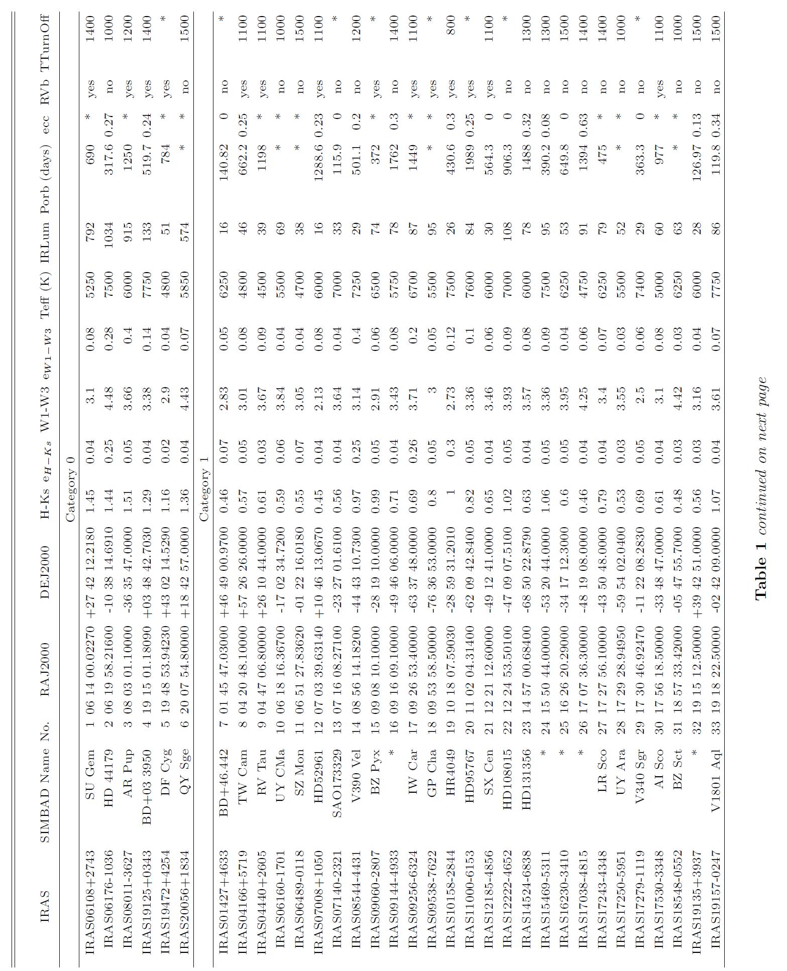
The Journal of Science Extension Research – Vol. 2, 2023 education.nsw.edu.au 272
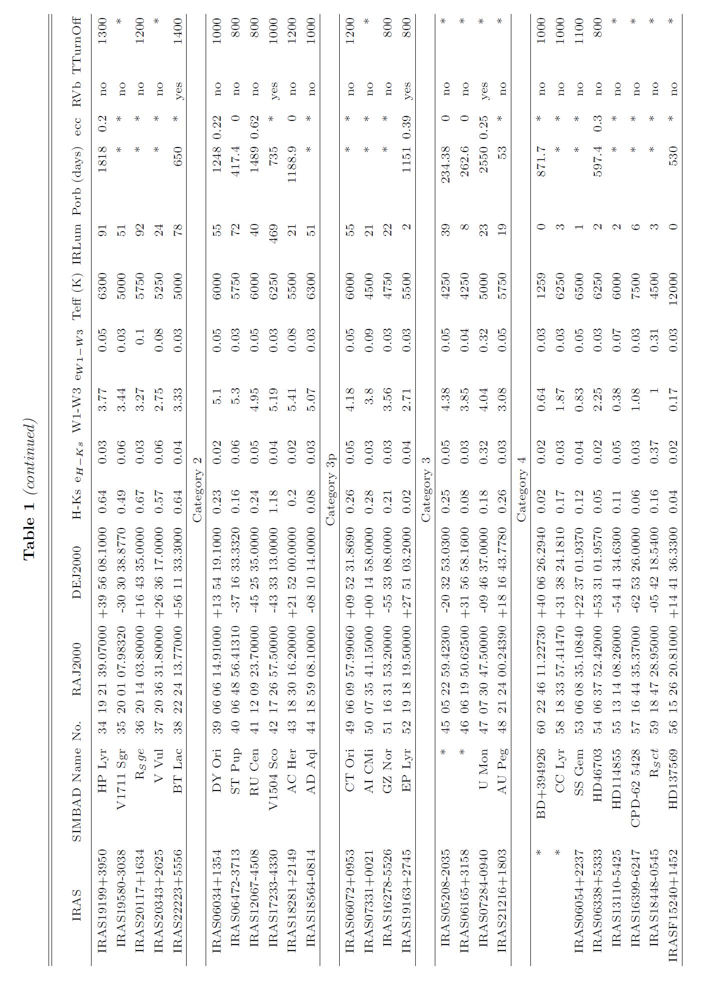
The Journal of Science Extension Research – Vol. 2, 2023 education.nsw.edu.au 273
B. FULL TARGET SAMPLE ABUNDANCES
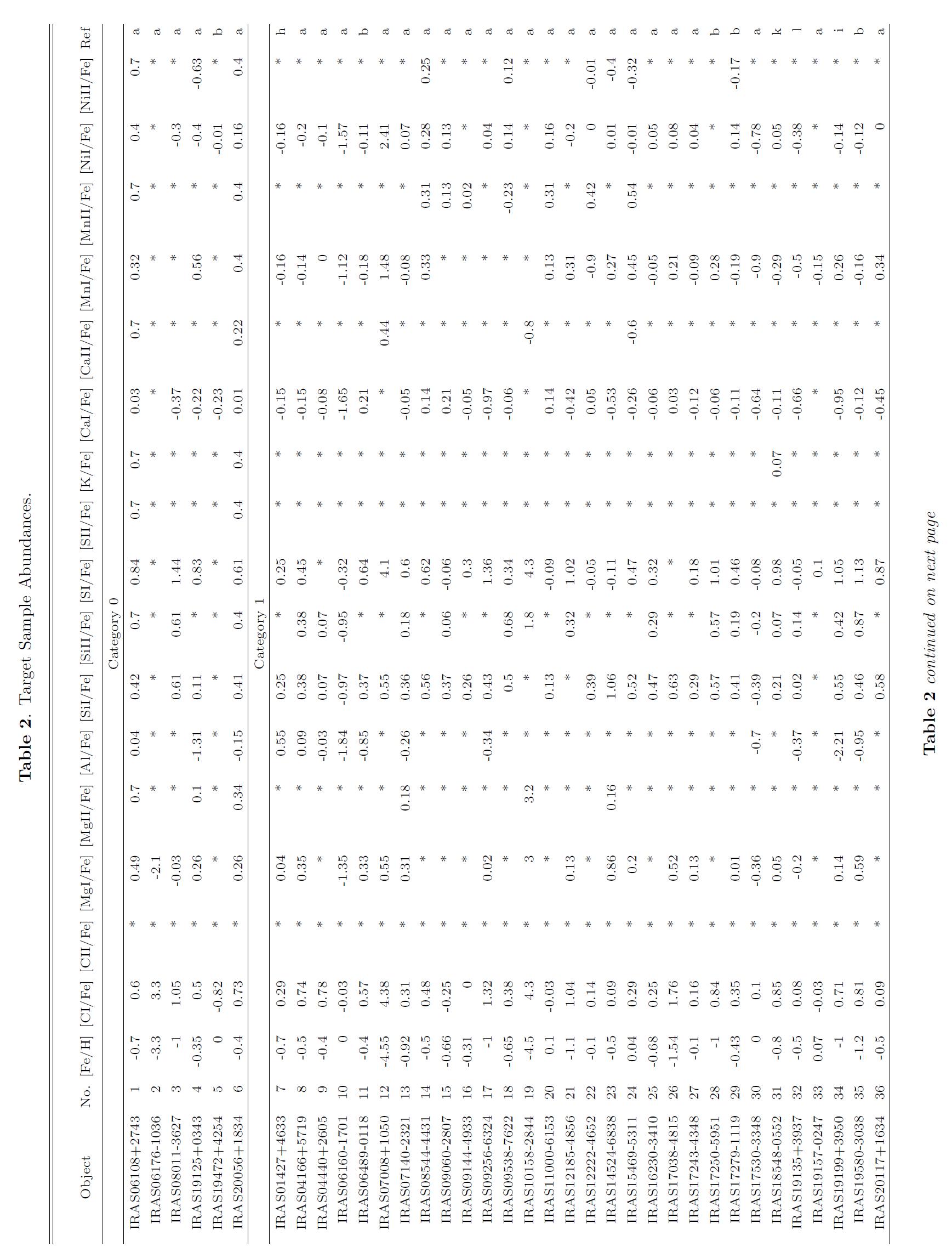
The Journal of Science Extension Research – Vol. 2, 2023 education.nsw.edu.au 274
The Journal of Science Extension Research – Vol. 2, 2023 education.nsw.edu.au 275
Figure 10. Adapted results from Wilson et al. (2022). Chemical abundances for the planet host (purple) and control (tan) samples. The chemical abundance displayed is shown in the upper left corner of each panel. The median error (±1σ) for each abundance is shown by the black error bar in the top right corner of each panel, and the dashed lines indicate the median abundances for the planet host sample (purple) and the control sample (tan).
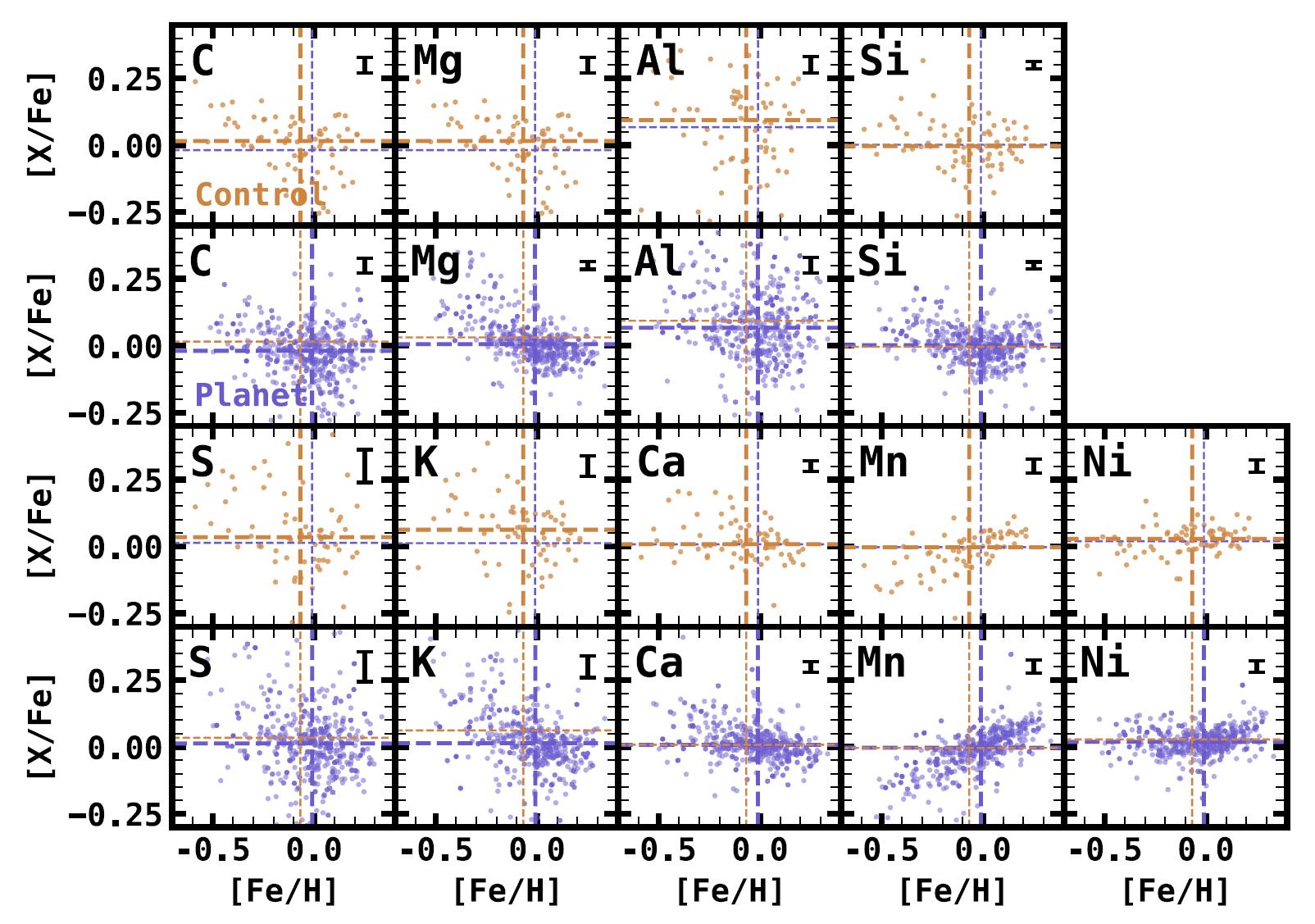
The Journal of Science Extension Research – Vol. 2, 2023 education.nsw.edu.au 276
Number of Rising Sequences of the Riffle and Overhand Card Shuffles
Leonardo Bruzze
Cherrybrook
Technology High School
This experimental study examined the number of rising sequences of the riffle and overhand card shuffles, intending to compare the two card shuffling strategies for use in casinos and social settings. By starting with two decks of 52 playing cards in their natural order, 40 riffle and 40 overhand shuffles were completed using separate decks, before recording the positions of the cards following each shuffle. The number of rising sequences was then determined by manually counting the number of sets of 3 or more cards that follow their natural order within the deck. While the mean value of the riffle shuffle was higher than the overhand shuffle, after performing a t-Test: Paired Two Sample for Means it was concluded that there was no statistically significant difference between the rising sequences of both card strategies. Thus, the null hypothesis was accepted, and the alternative hypothesis was rejected.
Literature Review
The process of randomising a deck of cards is essential to reduce predictability in the arrangement of the cards, with this issue being recognised by mathematicians, scientists and the general public alike. By ensuring the positions of the cards vary following each shuffle, the deck of cards can be dealt with fairly, minimising the chance of capitalisation by casinos. Furthermore, card cheats have taken advantage of predictable patterns in the arrangement of cards after being shuffled, calling attention to the need of mixing cards to a satisfactory extent (Aldous and Diaconis 1986, p. 345).
Randomisation of a deck of cards can be regarded as inducing a non-predictable permutation on the cards following a shuffle (Pemantle 1989, p. 38). This requires a shuffle technique and a shuffle count to be identified which contribute to
achieving the greatest variations in the card positions. This issue has been widely recognised by literature, including the study by Diaconis et al. (2013, p. 1693) whereby the variations of cards as a result of self-shuffling machines are analysed to draw practical application for games including poker and blackjack in casinos. Such paper identified the number of valleys in the permutation produced by the self-shuffler to be an indicator of the randomness of the cards, with no valleys being a uniform distribution (Diaconis et al. 2013, p. 1698). Their result of using a 10-shelf shuffler was found to be insufficiently random, recommending a 200-shelf machine to achieve total variation (Diaconis et al. 2013, p. 1717).
As demonstrated by the results of Diaconis et al., the problem of determining the number of shuffles to achieve total variation concerning automatic shufflers or computer modelling
The Journal of Science Extension Research – Vol. 2, 2023 education.nsw.edu.au 277
is comprehensively examined. The randomisation of cards from manual shuffling methods, however, has been minimally investigated. Since shuffling relies on the skill of the shuffler, the distribution of cards via the same shuffle will differ between different shufflers, pointing toward the importance of examining the effect of human shuffle practices on the arrangement of cards (Aldous and Diaconis 1986, p. 343). This is apparent due to the flaws involved with manual shuffling since single cards are dropped 50% of the time and pairs of cards are dropped 25% of the time while shuffling (Aldous and Diaconis 1986, p. 345). Thereby, the study conducted by Diaconis et al. was limited in its scope and application by disregarding the inconsistent and imperfect shuffle practices of humans despite the continued use of manual shuffling in casinos and other card-playing settings.
Pivotal research surpasses this method by comparing mechanical shuffling with the manual riffle shuffle, whereby 19 riffle shuffles were conducted to an initially ordered deck of cards (Silverman 2019, pp. 272-273). This study involved 5 randomness tests for both the manual and mechanical shuffles including rank correlation and the theory of rising sequences to determine the number of shuffles required to produce a random deck of cards. Whilst 12 automatic shuffles were required to mix a deck of cards to a satisfactory extent, only 8 hand shuffles were required for satisfactory mixing when comparing the statistical results of rising sequences (Silverman 2019, p. 295). Thereby, this study points towards the need to investigate the randomness of human shuffling practices, whilst is conversely limited in scope by directly focusing on just the riffle shuffle,
despite both the overhand and riffle shuffles being widely practised in society as the most popular shuffling methods (Pemantle 1989, p. 37).
This leads to the central question of whether card players should use the riffle or overhand shuffle when shuffling a deck of cards. The riffle shuffle involves separating the deck into two roughly equal parts and interlacing the cards as per the Gilbert-Shannon-Reeds model of shuffling, which can be mathematically defined as a permutation with 1 or 2 rising sequences (Aldous and Diaconis 1986, pp. 342-343). The overhand shuffle, on the other hand, requires the shuffler to slide small packets of cards out of the deck before successively depositing them back onto the top of the deck. A visual representation detailing how both the riffle and overhand card strategies can be performed is displayed below (Griffiths 2015).
Pemantle (1989, p. 49) suggested that between 1000 to 3000 overhand shuffles are required to randomise an ordered deck of cards as opposed to 7 riffle shuffles, thus highlighting that the riffle shuffle leads to the greater variation of the cards in a reduced number of shuffles as opposed to the overhand shuffle. The broad bounds of the recommended overhand shuffle count highlight the poor internal reliability of this study since the exact shuffle count to achieve
 Figure 1 Visual Representation of Riffle and Overhand Card Shuffles
The Journal of Science Extension Research – Vol. 2, 2023 education.nsw.edu.au 278
randomness was not determined. This 2000 shuffle range reduces the statistical significance of the study and thus causes it to stand as an unsatisfactory representation of the imperfect nature of human shuffling. Further, the results from Silverman’s (2019, p. 295) investigation reported imprecise results for a riffle shuffle after conducting various tests of randomness. He concluded that while 6 shuffles were required to achieve randomness when utilising the statistical test of rank-ordering, 10 shuffles were needed to achieve randomness when using the measure of runs relative to the mean (Silverman 2019, p. 295).
Thus, both Pemantle’s and Silverman’s studies are unreliable due to their inconsistent results when being compared. This possibly arises from the adopted measure of variation affecting the number of shuffles in achieving randomness, causing disparities to exist when identifying the precise shuffle count to achieve a random arrangement of cards. The key implication drawn from this research is the requirement to find a measure of randomness which best corresponds to unpredictability in the arrangement of cards. This may include the theory of rising sequences, which involves the identification of subsets of cards that are consecutively increasing following a shuffle. The number of such sequences between the two shuffle strategies can be compared to determine which strategy produces a more predictable arrangement of cards, hence holding critical importance in the card randomisation problem within society (Silverman 2019, p. 280).
Existing literature largely focuses on the randomisation of cards from the riffle shuffle or as a result of automatic
shuffling devices. The investigation into both the manual riffle and overhand shuffles, however, is critical due to their continued use in casinos and cardplaying settings. Literature also utilises different methods of determining randomness contributing to overall unreliable results, further pointing towards the necessity of completing further experimentation to gain an improved understanding of card randomisation. Consequently, by completing a designated shuffle count of both the riffle and overhand shuffles and utilising rising sequences as a measure of their variation, the randomisation of the initially ordered deck of 52 cards can be compared to determine the best strategy of card shuffling.
Scientific Research Question
Does the riffle shuffle or overhand shuffle produce the greater number of rising sequences of a deck of cards following the same shuffle count?
Scientific Hypothesis
Null Hypothesis: There is no statistically significant difference in the number of rising sequences produced by the riffle shuffle and overhand shuffle following the same shuffle count.
Alternative Hypothesis: There is a statistically significant difference in the number of rising sequences produced by the riffle shuffle and overhand shuffle following the same shuffle count.
The Journal of Science Extension Research – Vol. 2, 2023 education.nsw.edu.au 279
Methodology
The independent variable for this experiment was the shuffle number while the dependent variable was the number of rising sequences for each shuffling method.
There were no significant risks involved with the experiment, but regular breaks between shuffling and recording card positions were taken to reduce fatigue and eye strain.
Two identical decks of 52 playing cards in their natural order were used, starting with the Ace of clubs, Ace of spades, Ace of diamonds and Ace of hearts, and finishing with the King of clubs, King of spades, King of diamonds and King of hearts. The jokers or any instructional cards present were removed from the deck, as these cards are generally not used in casinos and many card games. These two decks were both new and of the same brand to ensure this variable was controlled, as different decks of cards would be made from different materials and of a different quality which could affect the shuffling of the cards.
The card shuffler started with one deck of cards, with a list from Ace of clubs to King of hearts from 1-52, forming a table with the numbers 1-40 as column headings to indicate the shuffle number. A single riffle shuffle was performed, before the positions of each card were recorded in the table (i.e. If the first card was a three of diamonds, a number ‘1’ would be recorded in the row corresponding to the card's initial position of ‘11’). This was completed for all 52 cards of the deck. Using the same deck of cards and the current rearranged order, the shuffler completed another riffle shuffle before recording the positions in the table. For
this shuffle and all subsequent shuffles, the halves of the deck were split into the same hands to ensure consistency in the shuffling. The same card shuffler completed this another 38 times, for a total of 40 card shuffles in the same environment.
After 40 riffle shuffles were completed, the card shuffler progressed to completing the overhand shuffle. The second deck of cards (new deck) was used, ensuring this variable was controlled as the previous deck underwent 40 shuffles which affect the quality of the deck of cards and could influence the results. The card shuffler constructed another table identical to the first to record the positions of the cards after each overhand shuffle. After a single overhand shuffle was performed, the positions of the 52 cards were recorded in the table.
Using the same deck of cards, the current rearranged order and starting with the deck of cards in the same hand, the same card shuffler completed another 39 overhand shuffles, for a total of 40 times in the same environment.
Once a total of 80 shuffles were completed (40 overhand shuffles and 40 riffle shuffles), and the positions of the cards after each shuffle were recorded, the number of rising sequences was determined. This estimator of randomness was chosen as it has decreased variability when compared to other randomness tests such as Kendall’s tau, enabling a statistical difference to be more aptly determined if one existed (Caudle 2018, p. 103). This required the shuffler to manually count the number of times in which a minimum of 3 cards are ascending within each shuffle.
The Journal of Science Extension Research – Vol. 2, 2023 education.nsw.edu.au 280
This is shown in Table 1, whereby the positions of cards are displayed after the 0th and 19th shuffle with each highlighted colour indicating a separate rising sequence. For example, the number ‘2’ under the heading ‘0th shuffle’ is indicative of the Ace of spades, and thus after the 19th shuffle, the Ace of spades has moved to position 6 in the deck.
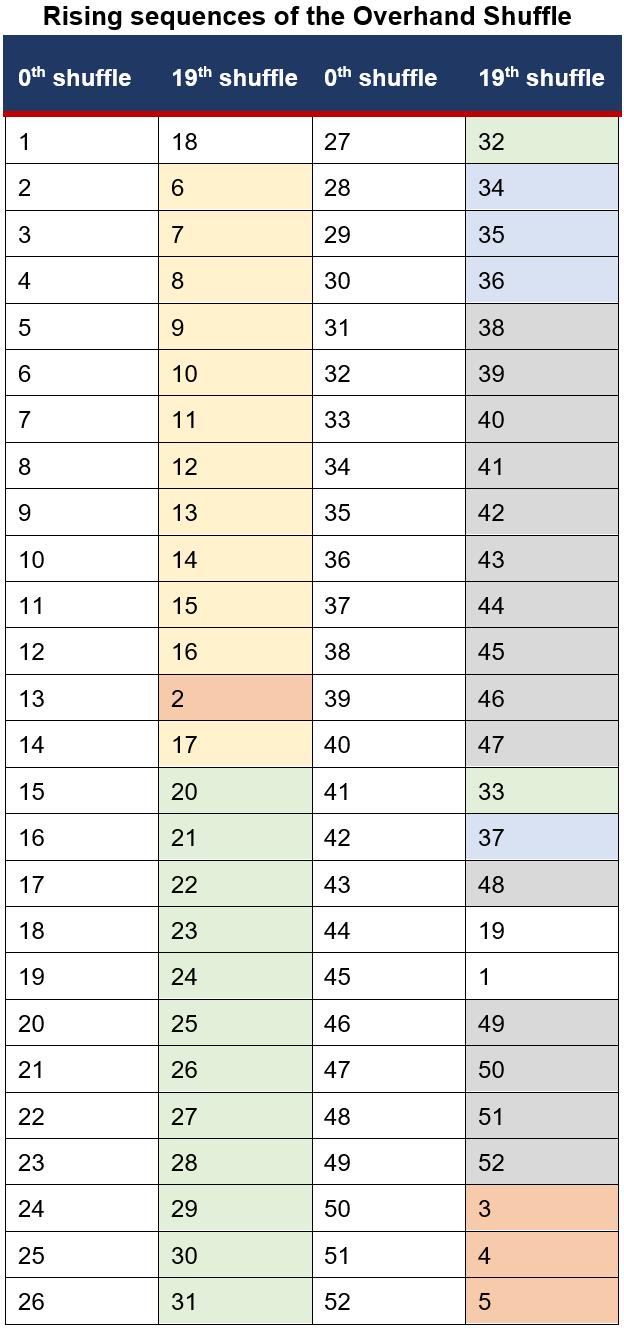
Thereby the 5 sets of rising sequences are:
1. 2-5 in orange
2. 6-17 in yellow
3. 20-33 in green
4. 34-37 in blue
5. 38-52 in grey
While the position numbers must be in ascending order, they do not need to be successive in the deck, so elements of a rising sequence can be separated by other elements (Silverman 2019, p. 280).
The mean number of rising sequences for both the riffle and overhand shuffles was calculated, before measures of variability such as variance and standard deviation were calculated, followed by a t-Test: Paired Two Sample for Means with significance determined at an alpha value of 0.05.
Table 1 Visual Representation of Rising Sequences of the Overhand Shuffle
The Journal of Science Extension Research – Vol. 2, 2023 education.nsw.edu.au 281
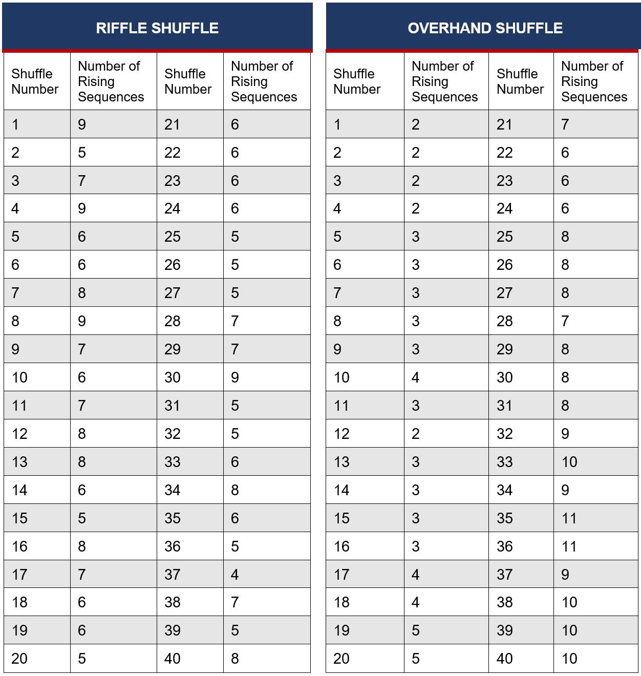
Results
Table 2 Rising Sequences of the Riffle Shuffle
The Journal of Science Extension Research – Vol. 2, 2023 education.nsw.edu.au 282
Table 3 Rising Sequences of the Overhand Shuffle
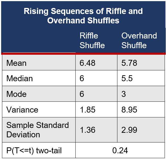
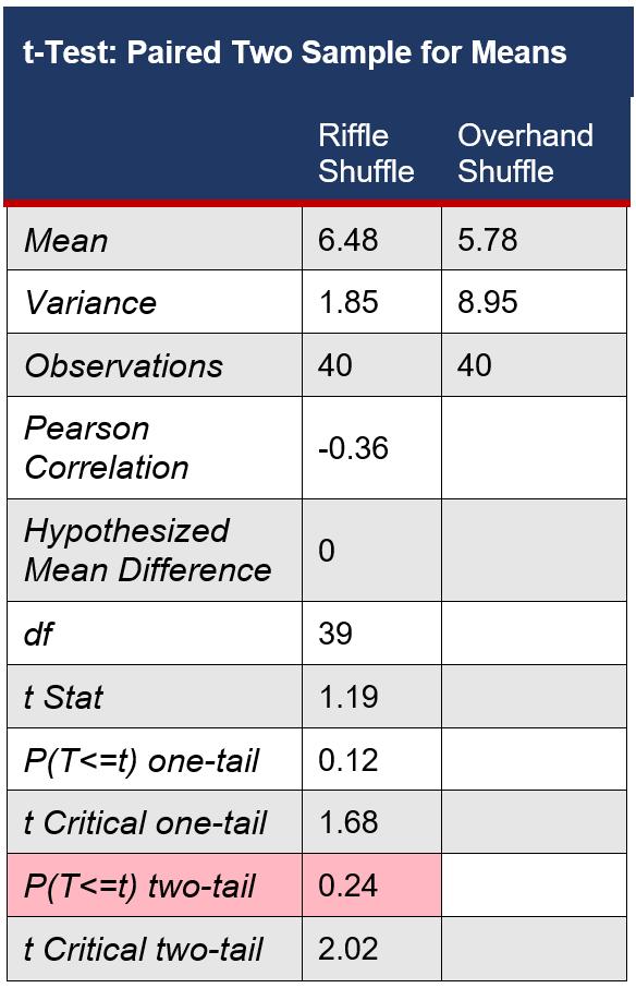
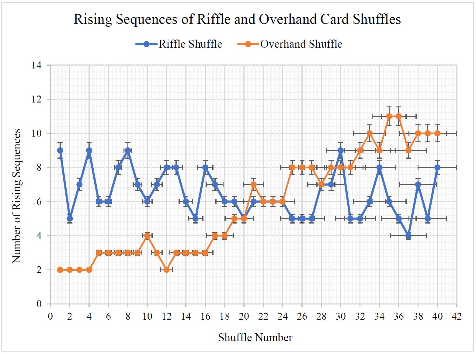 Table 4 Statistical Analysis of the Rising Sequences of Riffle and Overhand Shuffles
Table 5 t-Test: Paired Two Sample for Means
Table 4 Statistical Analysis of the Rising Sequences of Riffle and Overhand Shuffles
Table 5 t-Test: Paired Two Sample for Means
The Journal of Science Extension Research – Vol. 2, 2023 education.nsw.edu.au 283
Figure 2 Line Graph of the Rising Sequences of the Riffle and Overhand Shuffle
As demonstrated in Table 4, the mean value of rising sequences for the riffle shuffle (6.48) was higher than the mean value for the overhand shuffle (5.78) suggesting that the riffle shuffle produced a greater number of rising sequences than the overhand shuffle. Further, the overhand shuffle had a significantly higher variance (8.95) and sample standard deviation (2.99) as opposed to the riffle shuffle (variance of 1.85 and sample standard deviation of 1.36), demonstrating that the rising sequences of the overhand shuffle had a greater spread.
As displayed in Table 5, a ‘t-Test Paired Two Sample for Means’ was performed with a set alpha value of 0.05, thus it had a confidence interval of 95%. Since the P(T<=t) two-tail value of 0.24 was significantly higher than the alpha value of 0.05, it was concluded that the result was statistically insignificant. This had a confidence interval of only 76%, which was too low to be generally accepted within the scientific community as an accurate result.
Further, since the t Stat of 1.19 was less than the t Critical two-tail of 2.02, the null hypothesis was accepted, and the alternative hypothesis was rejected Therefore, there was no statistically significant difference in the number of rising sequences produced by the riffle shuffle and overhand shuffle following the same shuffle count.
Discussion
There are no credible studies that compare the rising sequences of the manual riffle and overhand card shuffles. While the study conducted by Silverman (2019, p. 295) suggested that 8 hand
shuffles using the riffle strategy are required for satisfactory mixing, this result was only compared to automatic shuffling rather than another manual shuffling strategy.
Neither this paper nor other credible sources which investigate shuffling practices draw comparisons between these manual shuffling methods. Thereby, the lack of scientific papers available causes this study to have poor reliability, and as such the statistically insignificant result drawn in this experiment is unreliable, requiring further similar studies to be conducted for it to be deemed a reliable result. This provides a route for future studies to explore, allowing contemporary scientific research to delve further into this card shuffling issue which has vast relevance to society.
In addition, previous studies such as the experiment conducted by Bayer and Diaconis (1992, p. 297) suggest that successive riffle shuffles should double the number of rising sequences, and as such after a third shuffle a deck should have 8 rising sequences. This experiment, however, demonstrates that after the first shuffle there were 9 rising sequences, followed by 5 after the second shuffle and 7 after the third shuffle, which is inconsistent with previous studies hence further reiterating the unreliable nature of this study.
Further, rising sequences are just one measure of randomness, and even if it was found that one shuffling method had more rising sequences based on a statistically significant result, one could not conclude that the strategy with more
The Journal of Science Extension Research – Vol. 2, 2023 education.nsw.edu.au 284
rising sequences leads to greater randomness in the arrangement of cards. This is because while the cards may not ascend in large portions, they may remain in a similar or unchanged position from the previous shuffle. As such, a variety of methods to determine the randomness should be used to achieve a more accurate result that aligns with the true value, yet the time constraints involved with this experiment limited the study’s ability to test multiple randomness indicators. As such, this study is limited in its practical application as it doesn’t suggest which shuffling method should be used in casinos and social settings.
Human shuffling practices wield a variety of random errors which affect the results achieved and reduce the accuracy of the experiment. This is because of the imperfect nature of human shuffling whereby each shuffle isn’t identical in nature even if it is performed by the same shuffler. This includes errors from dropping cards or mistakenly rearranging a part or whole of the deck, with inexperienced card shufflers dropping cards about 60% of the time while shuffling (Aldous and Diaconis 1986, p. 345). Further, the riffle shuffle requires the shuffler to divide the deck into roughly two equal parts before interleaving them, and this division would differ between shuffles resulting in different card placements. In addition, with each successive shuffle, the shuffler’s ability to perform the shuffling technique will become more fluent and efficient, which would skew the results and may cause a greater number of rising sequences.
Further, a larger sample size would also cause the result to have a greater level of internal reliability. Since only 40 riffle shuffles and 40 overhand shuffles were
completed due to time restraints, bias exists as the results are not truly representative of the number of rising sequences produced for each shuffling method. Thereby, to increase the reliability of this study a greater number of shuffles must be performed.
This is demonstrated in Figure 2. The line graph of the rising sequences of both the riffle and overhand shuffles shows inconsistencies in the result with many fluctuations across both shuffling methods. While the overhand shuffle demonstrates a positive relationship, the riffle
shuffle fluctuates across a similar number of rising sequences as the shuffle number increases. The length of the error bars also increased as the shuffle number increased which demonstrates the increasing number of errors in the results with a greater number of shuffles.
Conclusion
It is difficult to draw a definitive conclusion as many factors beyond the control of the shuffler, such as unintentionally dropping cards while shuffling, can cause the results to be inaccurate due to random errors. Furthermore, the time constraints associated with this study have resulted in a small sample size of data, requiring further experimentation under similar conditions which compares the riffle and overhand shuffles to achieve a more reliable result.
The mean value of the number of rising sequences of the riffle shuffle (6.48) is higher than that of the overhand shuffle (5.78), however, the result of the difference in the number of rising sequences between the two shuffling practices has proved to be statistically
The Journal of Science Extension Research – Vol. 2, 2023 education.nsw.edu.au 285
insignificant. This is because the P(T<=t) two-tail of 0.24 is higher than the defined alpha value of 0.05, causing the null hypothesis to be accepted and the alternative hypothesis to be rejected.
Future research can be influenced by this experiment, however, as it demonstrates the need to compare the rising sequences and other measures of randomness of the riffle and overhand shuffles. Further, technological advancements have resulted in the increased use of mechanical shuffling devices in casinos, pointing towards further direction for experimentation to compare the randomness between the riffle and overhand manual shuffling practices with a mechanical shuffle. This would allow for reduced predictability in card arrangements in casinos and social settings, thus being imperative in both the scientific community and amongst the general public.
References
Aldous, D. and Diaconis, P. 1986, ‘Shuffling Cards and Stopping Times’, The American Mathematical Monthly, vol. 93, no. 5, pp. 333-348, accessed 30 January 2022 from Taylor and Francis Online, ISSN; 0002-9890, <https://doi.org/10.1080/00029890.1986. 11971821>.
Bayer, D. and Diaconis, P. 1992, ‘Trailing the Dovetail Shuffle to its Lair’, The Annals of Applied Probability, vol. 2, no. 2, pp. 294-313, accessed 4 April 2022 from Institute of Mathematical Statistics, <http://www.jstor.org/stable/2959752>.
Caudle, K.A. 2018, ‘You betcha it’s random: riffle shuffling in card games –when is enough, enough?’, Teaching Statistics, vol. 40, no. 3, pp. 98-107,
accessed 29 May 2022 from Wiley Online Library, <https://doi.org/10.1111/test.12163>.
Diaconis, P., Fulman, J. and Holmes, S. 2013, ‘Analysis of Casino Shelf Shuffling Machines’, The Annals of Applied Probability, vol. 23, no. 4, pp. 1692-1720, accessed 23 January 2022 from Institute of Mathematical Statistics, <https://doi.org/10.1214/12- AAP884>.
Griffiths, S. 2015, ‘How to shuffle cards like a pro: Mathematician shows why the ‘riffle’ technique is more effective than the flashy ‘overhand’’, Daily Mail Australia, accessed 25 May 2022, <https://www.dailymail.co.uk/sciencetech/ article-3011046/How-shuffle-cards- likepro-Mathematician-shows-riffletechnique-effective-flashyoverhand.html>.
Pemantle, R. 1989, ‘Randomisation Time for the Overhand Shuffle’, Journal of Theoretical Probability, vol. 2, no. 1, pp. 37-49, accessed 5 February 2022 from SpringerLink, <https://doi.org/10.1007/BF01048267>.
Silverman, M.P. 2019, ‘Progressive Randomisation of a Deck of Playing Cards: Experimental Tests and Statistical Analysis of the Riffle Shuffle’, Open Journal of Statistics, vol. 9, no. 2, pp. 268-298, accessed 22 January 2022 from Scientific Research Publishing, ISSN; 2161-7198, <https://doi.org/10.4236/ojs.2019.92020>.
The Journal of Science Extension Research – Vol. 2, 2023 education.nsw.edu.au 286
Appendices

The Journal of Science Extension Research – Vol. 2, 2023 education.nsw.edu.au 287
Table 1 Positions of cards after 40 successive riffle shuffles

The Journal of Science Extension Research – Vol. 2, 2023 education.nsw.edu.au 288
Table 2 Positions of cards after 40 successive overhand shuffles
Segmenting Lungs Under Adverse Conditions Using MultiStage Transfer Learning: Preliminary Evidence of the Increased Generalisability when Retraining on Flipped Datasets
Minalu de Graaf Lambton High School
This investigation is a pilot study of performance of multi-stage transfer learning (MSTL) on a lung segmentation task within adverse conditions. Copies of a segmentation model were re-trained on different datasets of lung X-rays (rotated, flipped, 12.5% and 5% noise) and cross-evaluated on every dataset. It was concluded that most of the retrained models likely experienced covariate shifts with the exception of models trained on flipped datasets which show promising accuracy improvements that may indicate a route towards a retraining regime to increase generalisability. Additionally, noise as an adverse condition challenged the models the most due to the inconsistent scattering present on the object masks generated from the 12.5% noise test. Thus, this investigation gives insight into the thresholds of models trained on small datasets to perform under adverse conditions, adding to the knowledge base required to successfully integrate deep learning (DL) into the medical workflow.
Literature Review
The issue being addressed in this research is the occurrence of covariate shifts between the training and testing stages and live environment of DL models in radiology; MSTL will be utilised to minimise this issue. A model which detects lung areas for real world medical diagnostic applications must produce highly accurate results, which require significantly sized datasets. This is an issue in DL models’ development for medical image analysis as it requires expertise to create correct masks, greatly reducing the availability of accurate and sizable X-ray datasets (Quan et al., 2021). The rising importance of these issues resulted in studies on MSTL, which allows for the use of smaller
datasets to develop models of similar accuracy (Ausawalaithong et al., 2018), aiming to minimise the occurrence and effect of covariate shifts (Wang & Schneider, 2014). MSTL has a limited number of studies which analyse the application of this approach and its accuracy as a result of only recently being applied to medical imaging. However, transfer learning (TL) has ample research surrounding it within this field, which will be evaluated alongside studies focused on MSTL due to their similar methodologies.
Raghu and coworkers (2019) claim that knowledge surrounding the effect and application of TL is vital for the changing nature of the clinical workflow as the computational strain of complex models is too strong. When studying the literature,
The Journal of Science Extension Research – Vol. 2, 2023 education.nsw.edu.au 289
clashing results and conclusions were drawn between journals regarding the performance of TL models in clinical settings, for instance Alzubaidi and coworkers (2020) confidently note that TL significantly increases the performance of models by 2.8-11% (depending on the methodology employed), whereas Raghu and coworkers (2019) claim that there was no substantial improvement in performance due to TL, as the difference was under 1% for most of their results. The specified nature of DL models is likely the cause of this disparity between these published performances.
Investigations on Transfer Learning:
An investigation published in 2019 by Raghu and coworkers studied the effect of TL on a multitude of models and found that model training set size is a large factor in the effectiveness of TL. The initial methodology tested large ImageNet models against smaller custom-made CNN models, however, it branched out to explore the hidden representation unveiled by TL in the smaller models, depicting a change while training, similar in nature to a covariate shift.
In Figure 1, a distinct shift can be observed between (e) and (f) which correspond to the models with the smaller training set; Raghu and coworkers (2019) claim that this may be due to overparameterisation. Hence, the performance of these models were slightly improved as this phenomenon increased accuracy along with the time taken to train the given models (Godasu et al., 2020). As suggested by Godasu and coworkers (2020), MSTL is a possible solution for this issue, claiming that it allows models to shorten the
traditionally long training time, extended epochs and expensive computations. Ultimately, the study found that models trained on >200 000 images were largely unaffected by TL, whereas models trained on <5000 images depicted an accuracy increase of a few percent due to the occurrence of overparameterization as a result of changes similar to covariate shifts, highlighting a potential opportunity to investigate the impact of this effect on model training methodology.
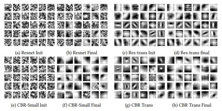 Figure 1: the visualisation of filters at initialisation and after training (Raghu et al., 2019)
The Journal of Science Extension Research – Vol. 2, 2023 education.nsw.edu.au 290
Investigations on Multi-Stage Transfer Learning:
Ausawalaithong and coworkers (2018) tested the performance of MSTL models against a TL base model. Within their methodology, three different datasets were utilised to re-train four models in varied ways. One of these datasets was the JSRT Dataset, which will be used in this investigation as well. To increase the reliability of each model’s performance, Ausawalaithong and coworkers (2018) performed a 10-fold cross-validation, which splits up the dataset to testing and training sets to estimate the classification ability of learning models. This procedure will be incorporated into the methodology of this investigation as it is an effective measure taken to minimise the difference between larger and smaller datasets.
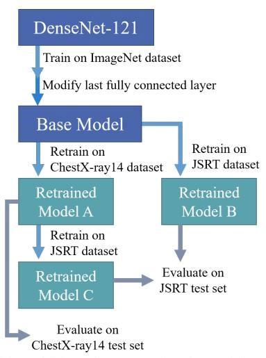
Within Ausawalaithong and coworkers' (2018) methodology, it states that the training images were randomly flipped horizontally for Model A, randomly rotated by 30 degrees for Model B and randomly flipped horizontally and rotated 30 degrees for Model C. This method of data augmentation is performed to increase the size of the datasets and simulate the adverse conditions of a live environment. However, this randomness may skew the performance of the models in unpredictable ways, hence, this investigation will control these variables by investigating the effect of individual adverse conditions. Ausawalaithong and coworkers (2018) claim that re-training a model to fit around specific conditions results in better performance. However, a notable issue encountered was overfitting in Model C, which resulted in the model’s lower accuracy in detecting the exact position of the cancer.
A similar investigation conducted by Samala and coworkers (2018) used MSTL to successfully train an algorithm using datasets in a similar auxiliary domain to the target of breast cancer detection. This yielded complementary results to Ausawalaithong and coworkers’ investigation (2018). In their two-stage approach, the model was trained using non-target data, followed by fine-tuning using the target dataset. The performance of this MSTL model was compared to a TL model. The TL model’s performance had 0.85±0.05 accuracy and the MSTL model outperformed this with 0.91±0.03 accuracy, alongside reducing the standard deviation of the results. Supporting the results from Ausawalaithong and coworkers (2018) by depicting the ability of MSTLs to generalise more effectively than standard DLs and TLs.
Ultimately, the literature demonstrates that MSTL has the potential to be used as a source of computationally smaller CADx in the clinical environment. However, the results of some studies are inconsistent
Figure 2 Schematic representation of methodology (Ausawalaithong et al., 2018)
The Journal of Science Extension Research – Vol. 2, 2023 education.nsw.edu.au 291
due to covariate shifts and the subsequent poor generalisation; hence, this investigation will aim to develop four models which are retrained and tested on small datasets to examine the effect of covariate shifts on model performance
Scientific Research Question
To what extent can multi-stage transfer learning increase the performance of lung area-detecting models under adverse
Variables
conditions (i.e., rotated, noisy and flipped images) when analysing X-ray images of chests?
Scientific Hypotheses
H0: The ability of the base and restrained models to generalise will not be significantly different.
HA: The retrained models will be able to generalise better than the base model.
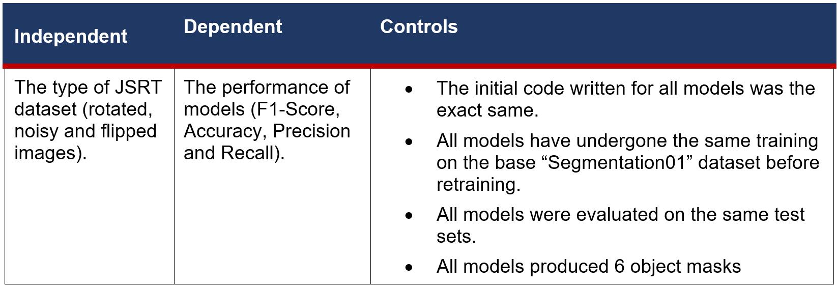
Table 1: Investigation variables examined during model training, testing and evaluation.
Methodology
Dataset Creation and Processing:
The set of 60 lung X-rays and corresponding segmentation masks used in this study were sourced from JSRT (Japanese Society of Radiological Technology & Japanese Radiology Society, 1998), which has a collection of open source datasets of lung X-rays. A small dataset was required to be able to test the effect of MSTL on model performance, therefore, the “Segmentation01” dataset was used from the miniJSRT set. Manual augmentation was performed using Adobe Photoshop’s filter tool and Free Transform tool to create additional rotated(90, 180 and 270
degrees), noisy (12.5% and 5%) and flipped datasets. All images were randomly partitioned into train (80%), test (10%) and validation (10%) sets across all 5 datasets.
CNN Architecture:
To create an efficient, small model, the Unet architecture and its number of fully connected layers and kernel size (Shallue & vanderburg, 2018) was most appropriate for this task. The primary alteration made to this architecture is the addition of padding on both the contracting and expansive paths to ensure that no border pixels are lost when passing through convolutions. The images were down-sampled, with maximum pooling between each
The Journal of Science Extension Research – Vol. 2, 2023 education.nsw.edu.au 292
convolutional layer, followed by upsampling paired with up-convolutions between each of these layers. ReLU (rectified linear unit) activation was used for all input and output layers, in addition, the output layer utilised sigmoid activation. The predicted mask and performance metrics were output by the models.
Implementation, Training & Testing:
The models were programmed in the Jupyter Notebook integrated development environment (IDE), and the models were trained on a school-provided device with an i7 CPU and a NVIDIA GPU to train the models in a feasible time frame. The environment installed onto the IDE was sourced from Portilla and coworkers (2021) which included the following libraries:
The Base model was trained on the untouched dataset; this was used as the starting point to retrain each of the other 4 models. The Rotated, Flipped, 12.5% and 5% Noise models were retrained on their respective datasets from copies of the Base model. As shown in Figure 3 all models were evaluated against every test set to measure their performances on each under each condition using a methodology inspired by Ausawalaithong and coworkers (2018); model performance was assessed by performing a right-tailed T-test with the performance of the Base model as the global control.
 Table 2: Machine Learning and Python Libraries used to build each model.
The Journal of Science Extension Research – Vol. 2, 2023 education.nsw.edu.au 293
Results
The four most effective measures of model performance are Accuracy, F1score, Recall and Precision; the mean and standard deviation was recorded to summarise the results. F1-score and Accuracy are the most representative
metrics due to the F1-Score punishing large differences in Precision and Recall, thus, they were the only two metrics used in the statistical tests to evaluate model performance. These metrics of all models examined are shown in Table 3 and the trends apparent are summarised in Table 4.
 Figure 3: Schematic representation of the training, testing and evaluating process
The Journal of Science Extension Research – Vol. 2, 2023 education.nsw.edu.au 294
Table 3: The mean and standard deviation of the Accuracy, F1-Score, Recall and Precision of all model performances.
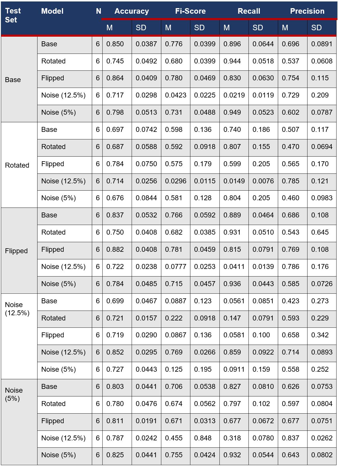
The Journal of Science Extension Research – Vol. 2, 2023 education.nsw.edu.au 295
Hypothesis Testing:
Right tailed t-tests assuming equal variances with an alpha value of 0.05 were performed between the Base model performance and all others individually for each test set. These compared the F1Scores (Table 5) and the Accuracy (Table 6).
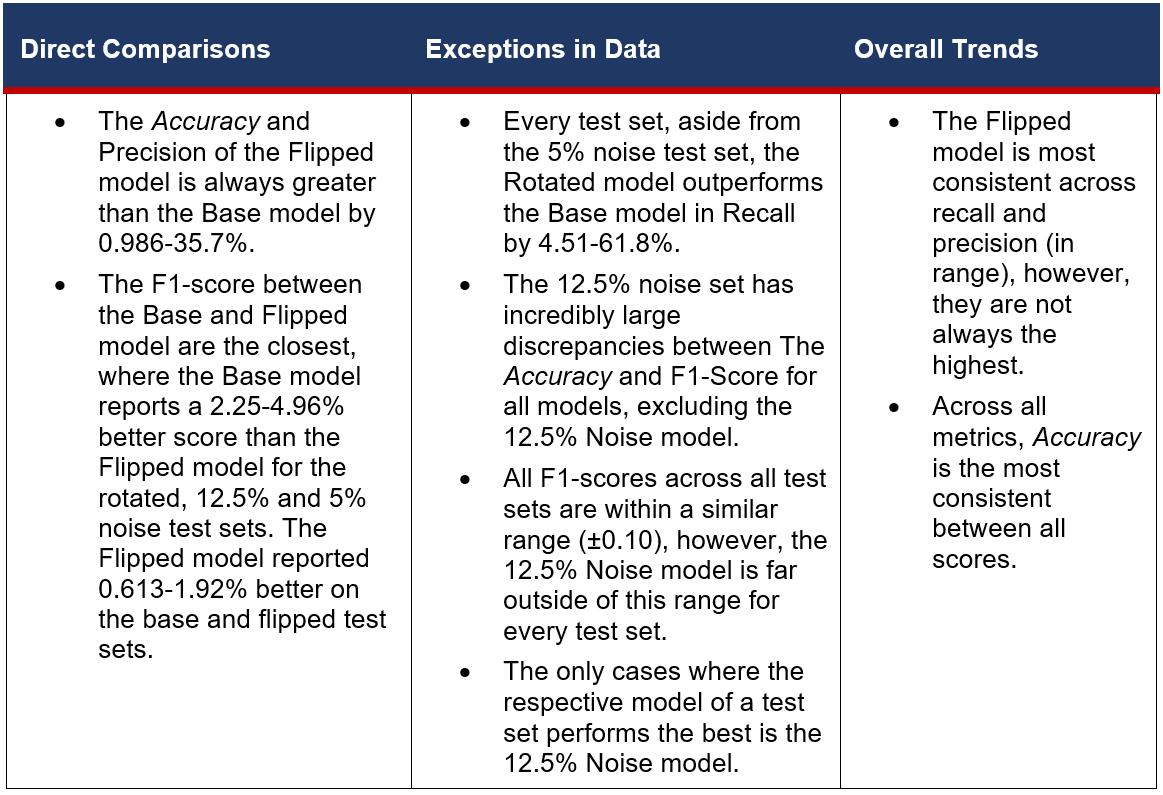
The Flipped model performed statistically significantly better than the Base model on the base (Flipped: M = 0.864, SD = 0.0409, Base: M = 0.850, SD = 0.0387) and rotated (Flipped: M = 0.784, SD = 0.0750, Base: M = 0.697, SD = 0.0742) test sets (Flipped on base test set: t(6) = 2.26, p = .0238 and Flipped on rotated test set: t(6) = 1.85, p = .0467) when evaluated for Accuracy. However, when
evaluated for the F1-score, the Base model outperformed most of the other models. For F1-Score, the Rotated model (t(6) = 1.95, p = .0402) and 12.5% Noise model (t(6) = 0.353, p = 1.39E-07) had a statistically significant improvement in the 12.5% noise test set (Base: M = 0.0887, SD = 0.123, Rotated: M = 0.222, SD = 0.0918, 12.5% Noise: M = 0.769, SD =0.0266). The mean F1-score and the mean Accuracy of the retrained models in 14 out of 16 cases were found to not be significantly improved over the Base model’s performance. This suggests that the retrained models as a whole had poor ability to generalise, leading to the null hypothesis being accepted. However, there are some notable anomalies which defy this trend that will be further discussed in the discussion.
Table 4: Trends found from the Accuracy, F1-Score, Recall and Precision of all model performances data reported in Table 4.
The Journal of Science Extension Research – Vol. 2, 2023 education.nsw.edu.au 296
*Underlined values indicate the p-values which were under the alpha value.
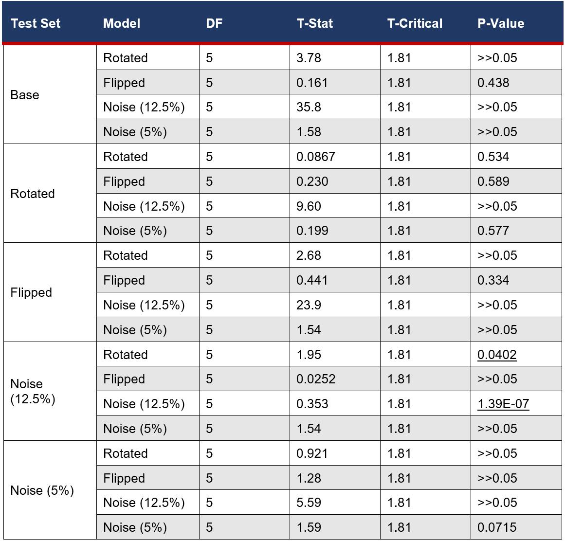 Table 5: The results of the statistical right-tailed T-test, evaluating the F1-Score for each model on each test set. Alpha = 0.05.
The Journal of Science Extension Research – Vol. 2, 2023 education.nsw.edu.au 297
*Underlined values indicate the p-values which were under the alpha value.
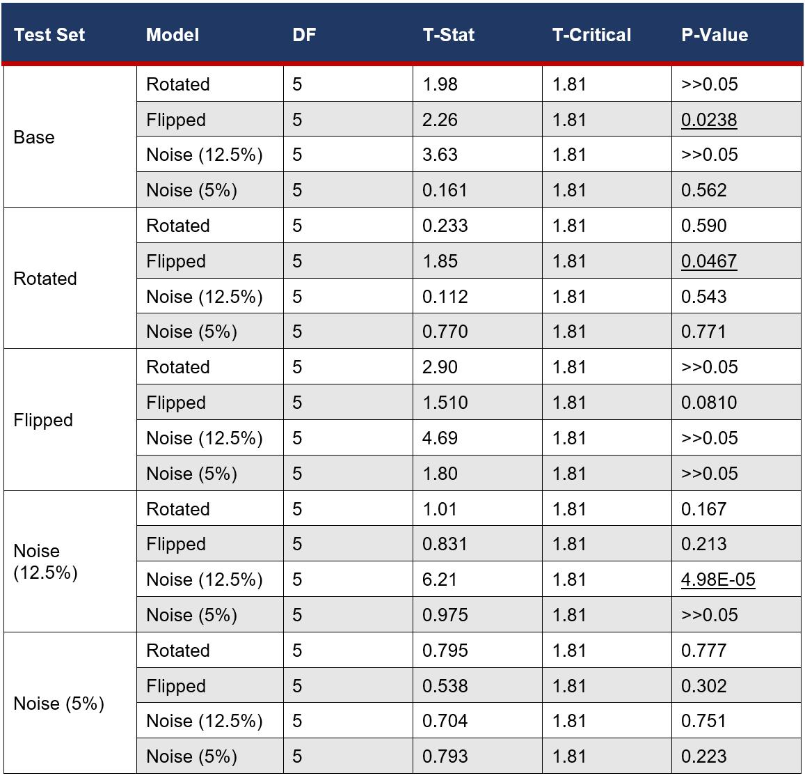
Visualisations:
In total, 150 images were produced by the models, therefore the most appropriate images from each test were randomly selected. These include the primary statistically significant evaluations and the overall best performing evaluation, providing a clear view of the visual correlations to the data. Each image contains the original X-ray (left),
the correct mask (middle) and the predicted mask (right).
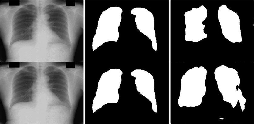 Table 6: The results of the statistical right-tailed T-test, evaluating the Accuracy for each model on each test set. Alpha = 0.05.
The Journal of Science Extension Research – Vol. 2, 2023 education.nsw.edu.au 298
Figure 4: Flipped model on base test set (top) vs Base model on base test set (bottom)
In Figures 4 and 5, the Flipped model outperformed the Base model in a statistically significant manner. Rather than exact precision and coverage, the Flipped model contains a significantly smaller amount of false positives (identification of lung tissue where there is none) compared to the Base model, thus creating a more accurate overlap with the correct mask. Additionally, there
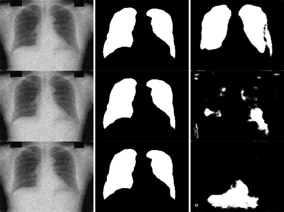
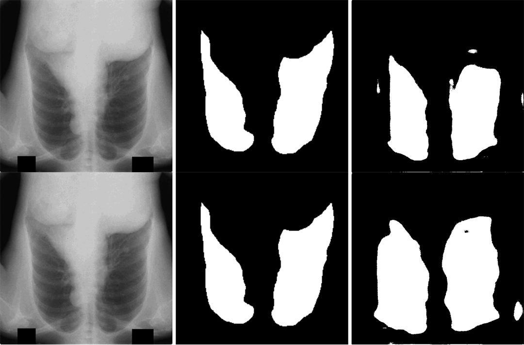
is less “random” scattering around the primary lung mask.

The overall best performance in both F1score (M = 0.781, SD = 0.0459) and Accuracy (M = 0.882, SD = 0.0408) is depicted in Figure 7 which shows the Flipped model evaluated on the flipped test set. Compared to the other models, Figure 7, depicts minimal false positives, however, it does contain one separate formation beside the left lung. From Figures 4, 5 and 7, it can be suggested that higher performing evaluations present minimised false positives and the object masks are more representative of the true shape of the lungs.
Discussion
The use of DL in medical environments provides an important addition to the toolset physicians use to analyse X-rays by introducing unbiased analysis. However, the inability for most models to effectively generalise is a major barrier for its implementation into the medical workflow (Lundervold & Lundervold, 2019). Therefore, understanding the interactions between models and adverse conditions (modelling real life) is important to increase their generalisability for its use in the clinical environment.
The retrained models did not perform better than the Base model on their respective sets aside from the 12.5% Noise model. This is a likely example of covariate shifts resulting in poor generalisation in a testing environment akin to a live environment. A vast majority of the models did not exceed the Base model’s performance in a statistically significant manner, however, the Flipped model had a statistically significantly better Accuracy than the Base model when tested against the base and rotated
Figure 5: Flipped model on rotated test set (top) vs Base model on rotated test set (bottom)
Figure 6: 12.5% Noise model on 12.5% noise test set (top) vs Rotated model on 12.5% noise test set (middle) vs Base model on 12.5% noise test set (bottom)
Figure 7: Flipped model on flipped test set (overall best performance in F1-Score and Accuracy)
The Journal of Science Extension Research – Vol. 2, 2023 education.nsw.edu.au 299
sets, additionally, it performed similarly to the Base model on all of the other tests. This may indicate that retraining a model on a flipped dataset can improve its generalisability. While promising, this must be investigated further to confirm this claim confidently.
With the chosen dataset, the “fine-tuning” of the models was performed by retraining on images with simulated adverse conditions instead of another task (e.g., classifying nodules). This can model MSTL to a certain extent, however, there are numerous limitations with this approach, evident in the varied data which does not entirely align with Godasu and coworker’s (2020) claims and Ausawalaithong and coworker’s (2018) findings. However, this data gives insight into the thresholds of models trained on small datasets to perform under adverse conditions. In future investigations, expanding the size of the training and test sets may allow for better generalisation by the retrained models. Despite this study’s altered scale of the MSTL, the methodology was valid and reliable because the widely cited and trusted Unet architecture was used to structure the models (Ronneberger et al., 2015). When each model generates object masks, the images are sampled over 512 times as the filters strides over each individual pixel to extract its features (transforming raw data into a numerical scale). This process is repeated at every convolutional layer where the image is down-sampled by systematically evolving filters, increasing its accuracy as no sampling errors are carried through the entire process. This process reduces the amount of parameters, and dropout layers randomly turn off neurons to regulate overfitting. Every convolutional layer extracts more information to
compare against the model’s knowledge base, thus, ensuring a reliable object mask is created. The metrics represent the extent to which the model succeeded at a correct segmentation. The standard deviation across all metrics averaged from 6 images is below 0.3, indicating that the generation of the object masks was consistent across each image.
The visualisations and the metrics give a unique insight into the relationship between these two mediums of evaluation, leading to the formation of numerous research questions about the obscure reaction of the models to a large amount of noise. The 12.5% noise dataset challenged all but the 12.5% Noise model the most, which is reflected in Figure 6 and the corresponding metrics. Some of the masks generated by these models did not have a single pixel of overlap with the true mask, whereas the other object masks consisted of random scattering, hardly ever representing the typical shape of lungs. It would be valuable to investigate if a threshold is evident in the ability of DL models to tolerate noise in a future study which focuses solely on retraining against increasingly noisy datasets. Expanding upon this, models could be retrained to classify nodules to determine if this effect translates into a model more akin to true MSTL models.
Ongoing investigation into numeric visualisation (weights) of the filters for each layer of the models has given preliminary indications that overparametisation is unlikely due to the similar weight values in each model. Therefore, to determine whether a covariate shift occurred, the models should be trained on larger datasets and tested on randomly augmented data. This
The Journal of Science Extension Research – Vol. 2, 2023 education.nsw.edu.au 300
process was beyond the timeframe and scope of this investigation, however, adding this process would allow for greater understanding of the commonly non-transparent internal mechanisms of DL models.
Conclusion
This investigation has revealed the potential for retraining models on a flipped dataset to improve their ability to generalise. A Base model and 4 other retrained models (on flipped, rotated, 12.5% or 5% noise datasets) were cross evaluated on base, flipped, rotated, 12.5% and 5% noise test sets to compare their performances. Statistical evaluations found that the 12.5% Noise model outperformed the Base model’s accuracy and F1-Score on the 12.5% noise test set. Further, the Flipped model outperformed the Base model’s accuracy on the base and rotated test sets. As only the 12.5% Noise model outperformed the Base model on its respective test set, the null hypothesis was accepted, however, there is evidence supporting the claim that retraining models on purposefully flipped datasets can be advantageous by increasing generalisation. This finding provides strong evidence for further research into MSTL model retraining and testing involving larger datasets. Future investigation into the effect of noisy datasets on a true MSTL model which classifies lung nodules would unpack the abnormally large influence which noise had on this investigation’s models.
Acknowledgements
Thank you Mr. Nicholson for your continued support and advice in the creation of this investigation and solving programming problems, and Mr. Redding for providing the device to train the models and for the devoted help with programming problems.
Source Code Access
The repository containing the source code is accessed through the QR code below:

Reference List
Alzubaidi, L., Fadhel, M. A., Al-Shamma, O., Zhang, J., Santamaría, J., Duan, Y., & R Oleiwi, S. (2020). Towards a better understanding of transfer learning for medical imaging: A case study. Applied Sciences, 10(13), 4523.
Ausawalaithong, W., Thirach, A., Marukatat, S., & Wilaiprasitporn, T. (2018). Automatic lung cancer prediction from chest X-ray images using the deep learning approach. 2018 11th Biomedical Engineering International Conference (BMEICON), 1–5.
Cohen, J. P., Viviano, J. D., Bertin, P., Morrison, P., Torabian, P., Guarrera, M., Lungren, M. P., Chaudhari, A., Brooks, R., Hashir, M., & others. (2021). TorchXRayVision: A library of chest X-ray datasets and models. ArXiv Preprint ArXiv:2111.00595.
Godasu, R., Zeng, D., & Sutrave, K. (2020). Transfer learning in medical
The Journal of Science Extension Research – Vol. 2, 2023 education.nsw.edu.au 301
image classification: Challenges and opportunities. Transfer, 5, 28–2020.
Hosny, A., Parmar, C., Quackenbush, J., Schwartz, L. H., & Aerts, H. J. (2018). Artificial intelligence in radiology. Nature Reviews Cancer, 18(8), 500–510.
Lundervold, A. S., & Lundervold, A. (2019). An overview of deep learning in medical imaging focusing on MRI.
Zeitschrift Für Medizinische Physik, 29(2), 102–127.
Prevedello, L. M., Halabi, S. S., Shih, G., Wu, C. C., Kohli, M. D., Chokshi, F. H., Erickson, B. J., Kalpathy-Cramer, J., Andriole, K. P., & Flanders, A. E. (2019). Challenges related to artificial intelligence research in medical imaging and the importance of image analysis competitions. Radiology: Artificial Intelligence, 1(1), e180031.
Quan, H., Xu, X., Zheng, T., Li, Z., Zhao, M., & Cui, X. (2021). DenseCapsNet: Detection of COVID-19 from X-ray images using a capsule neural network. Computers in Biology and Medicine, 133, 104399.
Raghu, M., Zhang, C., Kleinberg, J., & Bengio, S. (2019). Transfusion: Understanding transfer learning for medical imaging. ArXiv Preprint ArXiv:1902.07208.
Ronneberger, O., Fischer, P., & Brox, T. (2015). U-net: Convolutional networks for biomedical image segmentation. International Conference on Medical Image Computing and ComputerAssisted Intervention, 234–241.
Samala, R. K., Chan, H.-P., Hadjiiski, L., Helvie, M. A., Richter, C. D., & Cha, K. H. (2018). Breast cancer diagnosis in digital
breast tomosynthesis: Effects of training sample size on multi-stage transfer learning using deep neural nets. IEEE Transactions on Medical Imaging, 38(3), 686–696.
Schneider, S., Rusak, E., Eck, L., Bringmann, O., Brendel, W., & Bethge, M. (2020). Improving robustness against common corruptions by covariate shift adaptation. Advances in Neural Information Processing Systems, 33.
Shallue, C. J., & Vanderburg, A. (2018). Identifying exoplanets with deep learning: A five-planet resonant chain around kepler-80 and an eighth planet around kepler-90. The Astronomical Journal, 155(2), 94.
Wang, X., & Schneider, J. (2014)
Flexible transfer learning under support and model shift. Advances in Neural Information Processing Systems, 1898–1906.
Appendix 1 - Ethical Report
A large array of chest X-rays will be analysed by a CNN within this investigation to test the previously established hypothesis. The initial X-ray images contain confidential information regarding the patients (full name, age, condition etc.), thus, they are protected under the Privacy Act 1988. However, as all of the confidential information has been removed by JSRT (Japanese Society of Radiological Technology & Japanese Radiology Society, 1998) prior to its use in this investigation, thus, all of the patients’ confidential information was protected as it was never accessible at any stage of this investigation.
The Journal of Science Extension Research – Vol. 2, 2023 education.nsw.edu.au 302
Call for submissions
For the opportunity to have your students' research reports showcased in the next edition of the Science Extension journal, contact the Science 7-12 curriculum team.

Contact Science 7-12 curriculum team Science7-12@det.nsw.edu.au
NSW Department of Education