Predicting Solar Proton Event Magnitudes Using Vector Magnetic Data and a Neural Network Title of article

Predicting Solar Proton Event Magnitudes Using Vector Magnetic Data and a Neural Network Title of article

Vincent Ng – James Ruse Agricultural High School

Abstract

This study aimed to create and evaluate a neural network using vector magnetic data to predict the maximum proton flux at Earth caused by a future solar proton event (SPE), in which protons are accelerated to near-relativistic energies by solar eruptions. Two bidirectional long short-term memory (biLSTM) neural networks were developed to investigate the SPEs in the NASA/NOAA Solar Energetic Proton List. Both networks used data samples obtained from the Spaceweather HMI Active Region Patches (SHARPs) as input, however, the maximum proton flux of SPEs outputted was linearly scaled in one network and logarithmically scaled in the other. By analysing the ratio of underestimations to overestimations and comparing the error of the predictions made by these neural networks to the corresponding errors for baseline models with no skill, it was evident that the neural networks created in this study were not sufficiently accurate to be used for realworld applications.

Introduction

Solar proton events (SPEs) occur when protons are accelerated to nearrelativistic energies by solar eruptions. These events generate a flux of protons, measured in proton flux units (pfu), which may be directed at the Earth. The SWPC (Space Weather Prediction Centre) defines the start time of an SPE as the first of three consecutive data points where the flux of protons with energies greater than 10 MeV as measured by the Geostationary Operational Environmental Satellites (GOES), which orbit the Earth, is at least 10 pfu (National Oceanic and Atmospheric Administration [NOAA] 2022). SPEs can cause damage to the technical systems of space probes outside Earth’s magnetosphere and produce radiation which may be lethal to astronauts and affect passengers and flight crews on polar airline routes.

Additionally, large SPEs can ionise, excite, and dissociate atoms and molecules in the atmosphere, which can lead to ozone depletions in the polar upper stratosphere (Schwenn 2006).

Researchers have approached the problem of SPE prediction by developing empirical models with varying inputs. SPEs correlate with coronal mass ejections (clouds of ionised gas ejected from the Sun) and solar flares (sudden bursts of electromagnetic radiation emitted by the Sun) (Anastasiadis et al. 2019), so empirical prediction models have been developed using solar flare and coronal mass ejection data. For example, the ESPERTA model uses the flare location and soft x-ray and radio fluence (total amount of radiation flowing through an area) data, up to 10 minutes after the soft x-ray flux peak corresponding to a solar flare, to predict the probability of an SPE (Laurenza et al. 2018). Núñez et al. (2019) found that the UMASEP scheme, which predicts SPEs using the correlation between the intensity of soft x-rays emitted by the Sun and the differential proton fluxes (rate of proton flow through an area) measured near the Earth, could be adapted to take the intensity of extreme ultraviolet radiation as input. Núñez et al. (2020) built the UMASOD model, a decision tree model using flare and radio burst observational data to make a binary prediction on whether an SPE is expected. The most important attributes for this model were the soft x-ray fluence, the flare’s heliolatitude, and the maximum frequency of the type III radio bursts (radio emissions from the Sun associated with solar flares)

SPEs are affected by the Sun’s vector magnetic field because they occur when protons are accelerated by the energy release processes associated with the evolution of the Sun’s three-dimensional magnetic structure. Furthermore, these accelerated protons tend to move along the magnetic field lines emanating from the Sun because they are subject to the magnetic component of the Lorentz force, which acts on charged particles with a component of velocity directed perpendicularly to the local magnetic field (Vlahos 2019). Abduallah et al. (2022) developed a bidirectional long short-term memory (biLSTM) neural network to make a binary prediction of whether a solar Active Region (AR) would produce a SPE using data from the Spaceweather HMI Active Region Patches (SHARPs). SHARPs contain physical parameters describing the nature of the vector magnetic field within the Sun’s Ars

Whilst there have been predictive models developed to make binary or probabilistic predictions of whether an SPE will occur, there are fewer models designed to predict the maximum proton flux associated with a future SPE, and none using vector magnetic data. It would be useful to predict the maximum proton flux experienced at Earth because this determines the impact of an SPE on Earth, as outlined by the NOAA S-Scale (Appendix 1). For example, an S1 (minor) SPE is unlikely to have any biological or technological impacts, however, an S5 (extreme) SPE will expose astronauts outside space vehicles to high doses of radiation and may render satellites useless (NOAA n.d.). Therefore, the aim of this study is to create a neural network using vector magnetic data to predict the maximum proton flux experienced at Earth as a consequence of a future SPE. In practice, this predictive model would be used after another model has made a binary or probabilistic prediction indicating that an SPE is likely to occur

Scientific Research Question

Can vector magnetic data from the Sun’s ARs be used to predict the maximum solar proton flux that could be experienced at Earth as a consequence of a future SPE that will occur within the subsequent 24 hours?

Methodology

Constructing the Dataset

The NASA/NOAA Solar Energetic Proton List was used to create a database of SPEs that occurred from 1 May 2010 onwards, the date that the Helioseismic and Magnetic Imager (HMI) began collecting vector magnetic data. This database contained the start and maximum time, maximum proton flux, and NOAA AR for each SPE.

Vector magnetic data was obtained from the Spaceweather HMI Active Region Patches (SHARPs) created by Bobra et al. (2014), which is a data time series that documents 15 physical parameters of ARs with a 12-minute cadence (Figure 1, Appendix 2). These parameters are derived from the vector magnetograms taken by the HMI.

SPEs were omitted from the database of events if they were missing values for the start or maximum time, the maximum proton flux, or the NOAA AR. Additionally, SPEs were omitted if SHARP physical parameters could not be collected for at least 10 consecutive timesteps (points in time with data recorded). This reduced the number of events in the period 1 May 2010 to 30 June 2022 from 42 to 35 (Figure 4).

SHARP physical parameters from the AR associated with each SPE were collected for the 24 hours leading up to the event (Figure 2a). Given that the SHARP physical parameters have a 12-minute cadence, it was expected that there would be 120 timesteps for a 24-hour period, and thus 4200 timesteps for the 35 events investigated. However, because some ARs did not have data available for the entire 24-hour period preceding the event, there was only data for 3961 timesteps. This simulates how a neural network operating in real-life conditions may not have access to data for the full 24-hour period preceding a future SPE whose magnitude is to be predicted (Figure 2b).

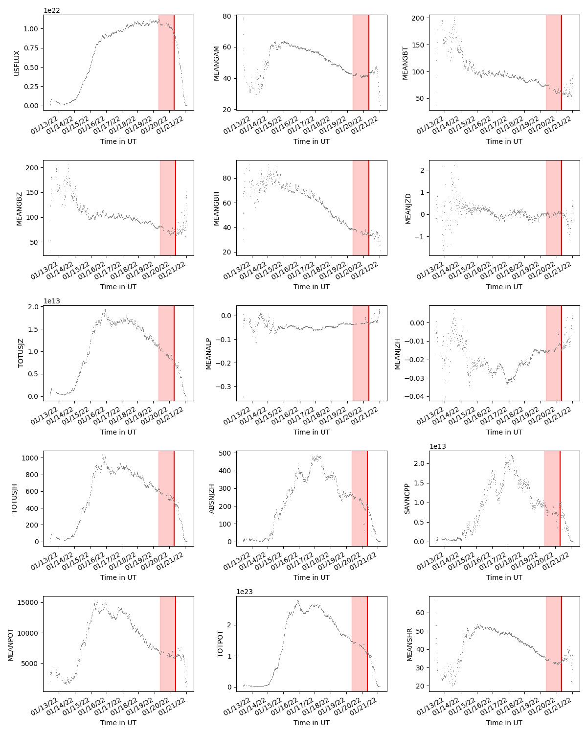
Figure 1: Plot of the fifteen SHARP physical parameters over time for the NOAA AR 2929 from 12 January 2022 10:36 UTC to 21 January 2022 00:36 UTC. The start time of the SPE (20 January 2022 08:00 UTC) (red line) and the 24-hour period leading up to it (red shaded area) have been added, using data from the NASA/NOAA Solar Energetic Proton List.

Figure 2: For each SPE, the neural network used the SHARP physical parameters from the associated AR for the 24 hours leading up to it. (a) When data was available beyond the 24 hours before the SPE, only the data from the 24 hours leading up to the SPE were considered. (b) When data was not available for the entire 24 hours leading up to the SPE, all data from timesteps preceding the start time of the SPE were considered.

Data samples were created from the SHARP physical parameters from 10 consecutive timesteps (Figure 3a), following the methodology used by Abduallah et al. (2022). These data samples were stored as 10×15 arrays (Figure 3b) to ensure that the inputs to the neural network had consistent data dimensions. The data samples overlapped with each other, meaning that each timestep formed part of multiple data samples. This ensured that the neural network could learn the relationships between consecutive timesteps, given that neural networks can only learn the relationships between the timesteps contained within a single data sample.

All data samples were stored in a single array to be inputted into the neural network. Each data sample was paired with its corresponding target value, the actual maximum proton flux measured for each SPE, which occupied the same index as the data sample in a second array containing the target values (Figure 3c).

Figure 3: (a) The data samples were created from the 15 SHARP physical parameters from 10 consecutive timesteps and overlapped with each other, so each timestep formed part of multiple data samples. (b) Each data sample was stored as a 10×15 array, with the first dimension corresponding to the 10 timesteps, and the second dimension corresponding to the 15 SHARP physical parameters. (c) The data samples and the target maximum proton flux values were each stored in an array. The data sample and target value for each SPE were paired by storing them in the same index in the respective array.

Training the Neural Network

The array of targets was duplicated and the target values in the duplicate array were rescaled by computing the logarithm (base 10) of the original target values, creating two arrays of target values: “linear targets” and “logarithmic targets”. Consequently, two neural networks were trained and compared: a “linear neural network” and a “logarithmic neural network”. The relationship between the maximum proton flux of an SPE and the impact of that SPE is logarithmic according to the NOAA S-Scale (Appendix 1). This means that the same magnitude of error in the predicted maximum proton flux will correspond to a greater difference in the impact of a weaker SPE (e.g. S1 (minor) SPE) compared to a stronger SPE (e.g. S5 (extreme) SPE). Thus, logarithmic scaling was chosen as a possible alternative to linear scaling because it was used by Boucheron et al. (2015) to predict the magnitude of solar flares, which exhibit similar logarithmic behaviour to SPEs.

The data samples were split into a training set and validation set. As there were relatively few data samples available for this study, a leave-one-out methodology, modified from the methodology used by AminalragiaGiamani et al. (2021), was used to validate the neural networks. In this “modified leave-one-out methodology”, the neural network was trained using the data from all but one of the SPEs in the event database, and validated using the data from the remaining SPE to estimate the accuracy of the neural network. This simulates real-life conditions where data samples from the SPE whose maximum proton flux is to be predicted would not be used to train the neural network. The arrays containing the data samples, linear targets, and logarithmic targets were each split into two arrays corresponding to the training and validation sets, creating six arrays in total: “training data samples”, “validation data samples”, “linear training targets”, “linear validation targets”, “logarithmic training targets”, and “logarithmic validation targets”.

Since the 15 SHARP physical parameters have different units and scales, the training and validation data samples were normalised using the min-max normalisation procedure used by Abduallah et al. (2022) (Appendix 3).

Bidirectional long short-term memory (biLSTM) networks were used because Abduallah et al. (2022) reported them to be the best machine learning method for the binary prediction and probabilistic forecasting of SPEs. The settings of the neural networks were chosen empirically (Appendix 4).

The accuracy was determined by training the neural network using the training data samples and targets and then calculating the validation loss as the mean average error (Equation 1) of the predictions made using the validation data samples.

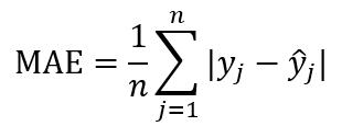
Equation 1: Mean Average Error, MAE

n = number of predictions

y_i = target maximum proton flux value for the jth SPE

predicted maximum proton flux value for the jth SPE

The linear and logarithmic neural networks were each compiled for 50 “epochs” (iterations over the training data samples and training targets) according to the modified leave-one-out methodology. The validation loss was calculated after each epoch. This was repeated ten times to reduce the impact of random errors. The optimal number of epochs to minimise the validation loss was found for both the linear and logarithmic neural networks.

The linear and logarithmic neural networks were each compiled for their optimal number of epochs according to the modified leave-one-out methodology. This was repeated ten times to reduce the impact of random errors. The predictions made using the validation data samples were stored in a database with the corresponding validation targets.

Baseline models were created to establish benchmarks for the neural networks. The linear baseline model predicted the maximum proton flux as the median of the linear training targets. The median linear baseline loss, the validation loss of this model, was calculated as the median of the mean average errors of the model predictions made by applying the modified leave-one-out methodology. The median was chosen as the measure of central tendency because there are obvious outliers in the baseline loss (Figure 6). A similar process was used to calculate the median baseline loss for the logarithmic neural network, using the logarithmic baseline model which predicted the log10(maximum proton flux) as the median of the logarithmic training targets.

Baseline models were created to establish benchmarks for the neural networks. The linear baseline model predicted the maximum proton flux as the median of the linear training targets. The median linear baseline loss, the validation loss of this model, was calculated as the median of the mean average errors of the model predictions made by applying the modified leave-one-out methodology. The median was chosen as the measure of central tendency because there are obvious outliers in the baseline loss (Figure 6). A similar process was used to calculate the median baseline loss for the logarithmic neural network, using the logarithmic baseline model which predicted the log10(maximum proton flux) as the median of the logarithmic training targets.

p=n/N

n = number of predictions with error less than the corresponding median baseline loss

N = total number of predictions

Equation 2: Proportion of predictions with error less than the median baseline loss of the corresponding baseline model, p

η=n_o/n_u

n_o = number of predictions that overestimated the maximum proton flux

n_u = number of predictions that underestimated the maximum proton flux

Equation 1: Ratio of predictions that overestimated the maximum proton flux to predictions that underestimated the maximum proton flux, η

Results

Figure 4: Frequency distribution of the maximum proton flux of the 35 SPEs in the database of events. The maximum proton flux has been plotted on a logarithmic scale to match the NOAA SScale (Appendix 1), which is used to classify the impact of solar radiation storms, such as SPEs. Of the 35 SPEs included in the database of events, 24 lay in the 10^1-10^2 pfu range corresponding to a S1 (minor) event, 7 lay in the 10^2-10^3 pfu range corresponding to a S2 (moderate) event, and 4 lay in the 10^3-10^4 pfu range corresponding to a S3 (strong) event.

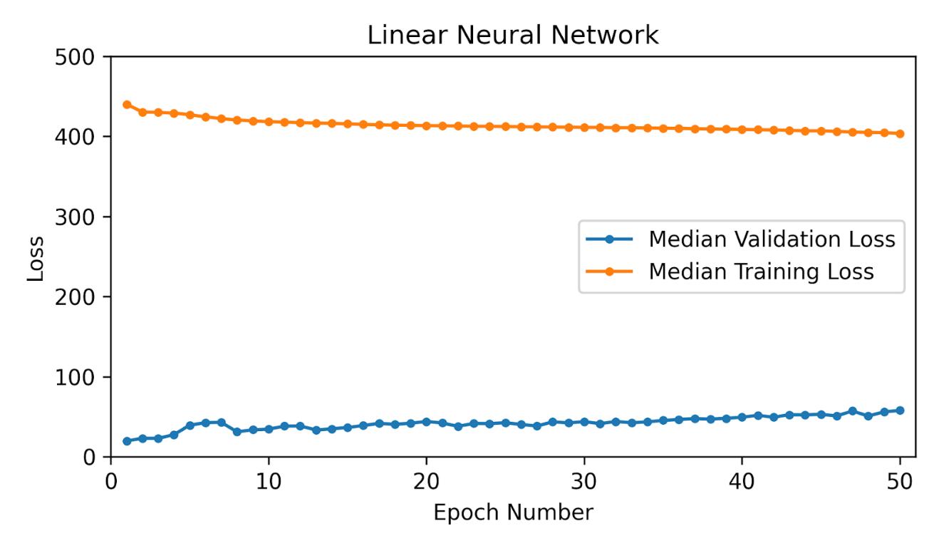
Figure 5: Learning curves for the linear neural network (top) and logarithmic neural network (bottom) over 50 epochs. The median training (orange) and validation (blue) losses were obtained for each epoch by repeating the modified leave-one-out methodology ten times.

A neural network is most accurate when the validation loss is minimised. Therefore, the linear neural network was most accurate when trained for 1 epoch, and the logarithmic neural network was most accurate when trained for 8 epochs (Figure 5).

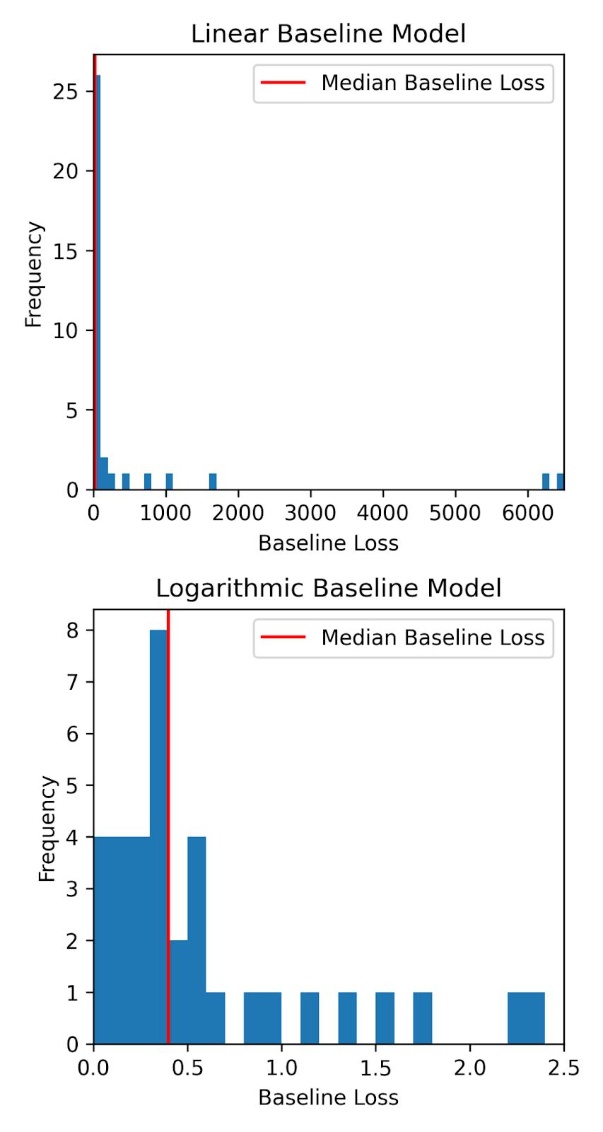
Figure 6: Histogram of the baseline losses obtained by applying the modified leaveone-out methodology to the linear baseline model (top) and logarithmic baseline model (bottom). The red line denotes the median baseline loss.

The median baseline loss was 21 for the linear baseline model and 0.40 for the logarithmic baseline model (Figure 6).

Figure 7: Histogram of the error of the predictions of the maximum proton flux made by the linear (top) and logarithmic (bottom) neural network. A negative error indicates that the neural network underestimated the actual value, and a positive error indicates that the neural network overestimated the actual value. The green area corresponds to the region where the neural network’s predictions are more accurate than the corresponding baseline model.

Figure 8: Histogram of the error of the linear neural network’s predictions of the maximum proton flux caused by actual S1 (minor) SPEs (top), actual S2 (moderate) SPEs (centre), and actual S3 (strong) SPEs (bottom). A negative error indicates that the linear neural network underestimated the actual value, and a positive error indicates that the linear neural network overestimated the actual value. The green area corresponds to the region where the predictions are more accurate than the linear baseline model.

Figure 9: Histogram of the error of the logarithmic neural network’s predictions of the maximum proton flux caused by actual S1 (minor) SPEs (top), actual S2 (moderate) SPEs (centre), and actual S3 (strong) SPEs (bottom). A negative error indicates that the logarithmic neural network underestimated the actual value, and a positive error indicates that the logarithmic neural network overestimated the actual value. The green area corresponds to the region where the predictions are more accurate than the logarithmic baseline model.

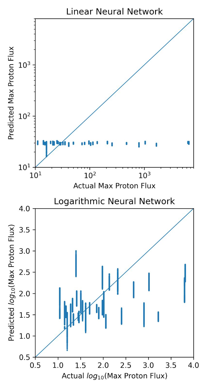
Figure 10: (Top) Plot of the target values of maximum proton flux against the predictions made by the linear neural network. (Bottom) Plot of the target values of log10(maximum proton flux) against the predictions made by the logarithmic neural network. For both plots, values closer to the line are more accurate, because the line represents an equality between the predicted and target values.

Table 1: Proportion of predictions with error less than the median baseline loss of the corresponding baseline model, p (Equation 2), reported for the predictions of each class of SPE. All values have been reported to two decimal places.

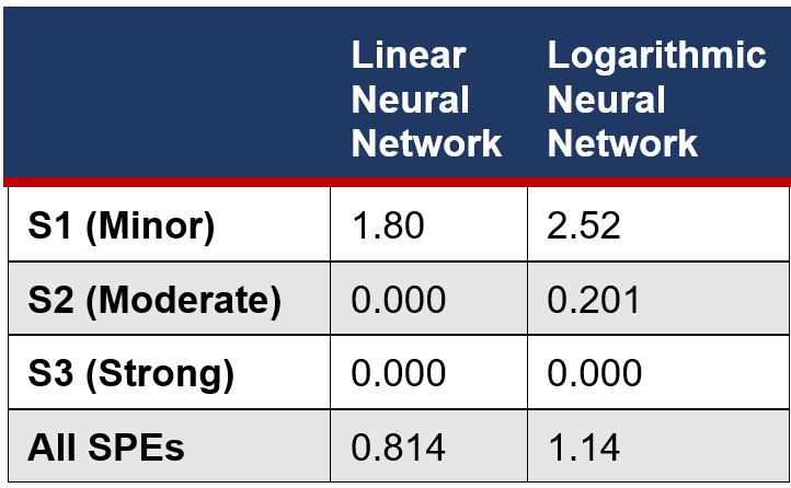
Table 2: Ratio of predictions that overestimated the maximum proton flux to predictions that underestimated the maximum proton flux, η (Equation 3), reported for the predictions of each class of SPE. Values greater than 1 indicate that overestimations were more common than underestimations, and values less than 1 indicate that underestimations were more common than overestimations. All values have been reported to three significant figures.

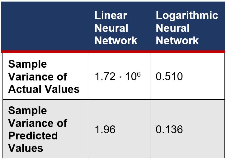
Table 3: Sample variance of the target values inputted into, and the predicted values outputted from the linear and logarithmic neural networks. All values have been reported to three significant figures.

Discussion

A neural network’s performance is quantified by its training and validation loss, the error of its predictions made using the data samples for training and validation respectively. Generally, the training and validation loss decrease as a neural network is compiled for more epochs, however, the validation loss will reach a minimum value where the neural network has been compiled for the optimal number of epochs. After this point, the neural network will overfit to the training data, meaning that it has become too specific to the training data to make accurate predictions using other input data (Figure 11). This trend was observed for the logarithmic neural network, which performed optimally when compiled for 8 epochs (Figure 5). Whilst the training loss for the linear neural network decreased as the epoch number increased, the validation loss did not decrease to a minimum value (Figure 5). It is unlikely that the linear neural network overfitted from the first epoch because this was not observed for the logarithmic neural network which was trained with the same volume of data. Instead, since the error of the predictions (especially the linear neural network) was negatively skewed (Figure 7), it is likely that the loss function chosen (mean average error) was not appropriate for quantifying the accuracy of the neural network (Pernot et al. 2020).

Figure 11: Typical learning curve for a neural network. The validation (blue) and training (orange) loss are plotted against the epoch number, and the optimal number of epochs is indicated by the dotted line. Figure is adapted from Vogl (2018).

Stronger SPEs, which cause higher maximum proton fluxes at Earth, occur less frequently than weaker SPEs, which cause lower maximum proton fluxes at Earth, because they are produced by rarer, more energetic solar eruptions. Additionally, solar activity varies according to solar cycles which have a periodicity of 11 years, and most SPEs used in this study occurred during Solar Cycle 24 (2008-2019), which was the weakest cycle of the past century (Nandy 2021). Therefore, the distribution of the maximum proton flux of the 35 SPEs in the database of events was positively skewed (Figure 4). This explains why the neural networks were more accurate when predicting weaker SPEs, with both neural networks predicting most S1 (minor) SPEs but no S3 (strong) SPEs with better accuracy than the baseline model, which simulated a model with no skill (Table 1). The lack of data for stronger SPEs also accounts for how the neural networks tended to underestimate the maximum proton flux for S2 (moderate) and S3 (strong) SPEs (Figures 7-9, Table 2). Additionally, the variance of the predicted maximum proton flux values was far less than the variance of the target values (Figure 10, Table 3), especially for the linear neural network, implying that the neural networks were unable to differentiate between stronger and weaker SPEs. Therefore, as the neural networks are intended to predict the impact of a SPE on Earth, neither would be useful in a real-life scenario because they would consistently underestimate the magnitude of stronger SPEs. Consequently, authorities would be unable to implement measures to mitigate the greater impact of these stronger SPEs on technologies and humans.

Clearly, the neural networks created in this study require more training data to accurately predict the maximum proton flux corresponding to an SPE. As SPEs rarely impact the Earth, with only 42 events recorded by NASA/NOAA since 2010, it is not feasible to wait until there is a sufficient volume of data to train and validate a neural network which can accurately predict SPEs. Additional vector magnetic data could be sourced using the Spaceweather MDI Active Region Patches (SMARPs) which is a data time series containing three of the SHARP physical parameters with a larger, 96minute cadence for the period January 1996 to October 2010. The SMARP data is derived from the line-of-sight magnetograms taken by the Michelson Doppler Imager (MDI) (Bobra et al. 2021b). Furthermore, additional SPEs could be sourced using the Space Weather Database Of Notifications, Knowledge, Information (DONKI), which includes SPEs detected by the Solar and Heliospheric Observatory (SOHO) and the Solar Terrestrial Relations Observatory (STEREO) in addition to those detected by the Geostationary Operational Environmental Satellites (GOES) that were used in this study. However, SOHO and STEREO do not orbit the Earth (Figure 12), so SPEs detected by these satellites may not be valid for creating a neural network designed to predict the proton flux at Earth. Alternatively, the neural network could be enhanced using an error penalisation method in which errors when making predictions for SPEs with higher maximum proton fluxes are weighted more than for SPEs with lower maximum proton fluxes, which are overrepresented in the data used in this study (Aminalragia-Giamani et al. 2021).

Figure 12: Positions of the Solar and Heliospheric Observatory (SOHO) and both Solar Terrestrial Relations Observatory (STEREO) spacecraft relative to Earth. The two STEREO spacecraft orbit the Sun along the Earth’s orbit path, with STEREO-A (labelled “Ahead”) orbiting ahead of the Earth and STEREO-B (labelled “Behind”) orbiting behind the Earth. SOHO is located at Lagrange Point L1, which lies 1.6 million kilometres towards the Sun from Earth, and orbits the Sun with the same orbital period as Earth.

Figure is reproduced from de Sadeleer (2013).

Conclusion

This study investigated the use of vector magnetic data to predict the maximum proton flux experienced at Earth due to an SPE. The SHARP physical parameters describing the magnetic structure in each of the Sun’s ARs were collected for the 24 hours prior to each SPE in the NASA/NOAA Solar Energetic Proton List and collated into data samples which were paired with their corresponding target maximum proton flux values. This dataset was used to train and validate a linear and logarithmic neural network, in which the target values were linearly and logarithmically scaled respectively, using a modified leave-one- out methodology where the neural networks were trained using the data from all but one of the SPEs, and validated using the data from the remaining SPE. The linear and logarithmic neural networks were benchmarked against the linear and logarithmic baseline models which predicted the maximum proton flux value with no skill.

The accuracies of the linear and logarithmic neural networks were maximised when they were compiled for 1 and 8 epochs respectively. Whilst the neural networks could predict the maximum proton flux for weaker SPEs (e.g. S1 (minor)) more accurately than the corresponding baseline models most of the time, they failed to generate accurate predictions for stronger events (e.g. S3 (strong)). Both neural networks generally underestimated the maximum proton flux caused by SPEs. In conclusion, neither neural network would be accurate enough to be used in a real-life scenario to alert authorities to a strong SPE likely to impact technologies and humans.

References

Abduallah, Y, Jordanova, VK, Liu, H, Li, Q, Wang, JTL & Wang, H 2022, ‘Predicting Solar Energetic Particles Using SDO/HMI Vector Magnetic Data Products and a Bidirectional LSTM Network’, The Astrophysical Journal Supplement Series, vol. 260, no. 1, viewed 15 May 2022, DOI 10.3847/15384365/ac5f56.

Aminalragia-Giamini, S, Raptis, S, Anastasiadis, A, Tsigkanos, A, Sandberg, I, Papaioannou, A, Papadimitriou, C, Jiggens, P, Aran, A & Daglis, I 2021, ‘Solar Energetic Particle Event occurrence prediction using Solar Flare Soft X-ray measurements and Machine Learning’, Journal of Space Weather and Space Climate, vol. 11, viewed 7 February 2022, DOI 10.1051/swsc/2021043.

Anastasiadis, A, Lario, D, Papaioannou, A, Kouloumvakos, A & Vourlidas, A 2019, ‘Solar energetic particles in the inner heliosphere: status and open questions’, Philosophical Transactions of the Royal Society A: Mathematical, Physical and Engineering Sciences, vol. 377, viewed 7 February 2022, DOI 10.1098/rsta.2018.0100.

Bobra, MG, Sun, X, Hoeksema, JT, Turmon, M, Liu, Y, Hayashi, K, Barnes, G & Leka, KD 2014, ‘The Helioseismic and Magnetic Imager (HMI) Vector Magnetic Field Pipeline: SHARPs - Space-Weather HMI Active Region Patches’, Solar Physics, vol. 289, no. 9, pp. 3549–3578, viewed 27 March 2022, DOI 10.1007/s11207-014-0529-3.

Bobra, MG, Sun, X & Turmon, MJ 2021a, mbobra/SHARPs: SHARPs 0.1.0 (202107-23), Zenodo, viewed 18 June 2022, DOI 10.5281/zenodo.5131292.

Bobra, MG, Wright, PJ, Sun, X & Turmon, MJ 2021b, ‘SMARPs and SHARPs: Two Solar Cycles of Active Region Data’, The Astrophysical Journal Supplement Series, vol. 256, no. 2, viewed 27 March 2022, DOI 10.3847/1538-4365/ac1f1d.

Boucheron, LE, Al-Ghraibah, A & McAteer, RTJ 2015, ‘Prediction of Solar Flare Size and Time-to-Flare Using Support Vector Machine Regression’, Astrophysical Journal, vol. 812, no. 1, viewed 15 July 2022, DOI 10.1088/0004637X/812/1/51.

Chen, Y, Manchester, WB, Hero, AO, Toth, G, DuFumier, B, Zhou, T, Wang, X, Zhu, H, Sun, Z & Gombosi, TI 2019, ‘Identifying Solar Flare Precursors Using Time Series of SDO/HMI Images and SHARP Parameters’, Space Weather, vol. 17, no. 10, pp. 1404–1426, viewed 15 July 2022, DOI 10.1029/2019SW002214.

Chollet, F 2018, Deep Learning with Python, Manning Publications Co., Shelter Island, NY, viewed 16 May 2022, https://tanthiamhuat.files.wordpress.com/ 2018/03/deeplearningwithpython.pdf

de Sadeleer, A 2013, ‘Power, Progress & Prestige: International Relations in Outer Space. A Study in Global Astropolitics, 1940s - 2030s’, Master’s thesis, Université catholique de Louvain, viewed 24 August 2022, https://www.researchgate.net/publication/ 315800396_Power_Progress_Prestige_In ternational_Relations_in_Outer_Space_A _Study_in_Global_Astropolitics_1940s__2030s

Kahler, SW & Ling, AG 2018, ‘Forecasting Solar Energetic Particle (SEP) events with Flare X-ray peak ratios’, Journal of Space Weather and Space Climate, vol. 8, viewed 11 April 2022, DOI 10.1051/swsc/2018033.

Laurenza, M, Alberti, T & Cliver, EW 2018, ‘A Short-term ESPERTA-based Forecast Tool for Moderate-to-extreme Solar Proton Events’, The Astrophysical Journal, vol. 857, no. 2, viewed 8 February 2022, DOI 10.3847/15384357/aab712.

Liu, C, Deng, N, Wang, JTL & Wang, H 2017, ‘Predicting Solar Flares Using SDO /HMI Vector Magnetic Data Products and the Random Forest Algorithm’, The Astrophysical Journal, vol. 843, no. 2, viewed 15 May 2022, DOI 10.3847/15384357/aa789b.

Liu, H, Liu, C, Wang, JTL & Wang, H 2019, ‘Predicting Solar Flares Using a Long Short-term Memory Network’, The Astrophysical Journal, vol. 877, no. 2, viewed 15 May 2022, DOI 10.3847/15384357/ab1b3c.

Liu, H, Liu, C, Wang, JTL & Wang, H 2020, ‘Predicting Coronal Mass Ejections Using SDO/HMI Vector Magnetic Data Products and Recurrent Neural Networks’, The Astrophysical Journal, vol. 890, no. 1, viewed 15 May 2022, DOI 10.3847/1538-4357/ab6850.

Murray, SA 2018, ‘The Importance of Ensemble Techniques for Operational Space Weather Forecasting’, Space Weather, vol. 16, no. 7, pp. 777–783, viewed 5 February 2022, DOI 10.1029/2018SW001861.xt

Nandy, D 2021, ‘Progress in Solar Cycle Predictions: Sunspot Cycles 24-25 in Perspective’, Solar Physics, vol. 296, no. 3, viewed 12 August 2022, DOI 10.1007/s11207-021-01797-2.

National Oceanic and Atmospheric Administration n.d., NOAA Space Weather Scales, viewed 31 July 2022, https://www.swpc.noaa.gov/noaa-scalesexplanation

National Oceanic and Atmospheric Administration 2022, Solar Proton Events Affecting the Earth Environment, viewed 12 August 2022, ftp://ftp.swpc.noaa.gov/pub/indices/SPE.t

Núñez, M, Nieves-Chinchilla, T & Pulkkinen, A 2019, ‘Predicting wellconnected SEP events from observations of solar EUVs and energetic protons’, Journal of Space Weather and Space Climate, vol. 9, viewed 7 February 2022, DOI 10.1051/swsc/2019025.

Núñez, M & Paul-Pena, D 2020, ‘Predicting >10 MeV SEP Events from Solar Flare and Radio Burst Data’, Universe, vol. 6, no. 10, viewed 7 February 2022, DOI 10.3390/universe6100161.

Papaioannou, A, Sandberg, I, Anastasiadis, A, Kouloumvakos, A, Georgoulis, MK, Tziotziou, K, Tsiropoula, G, Jiggens, P & Hilgers, A 2016, ‘Solar flares, coronal mass ejections and solar energetic particle event characteristics’, Journal of Space Weather and Space Climate, vol. 6, viewed 29 March 2022, DOI 10.1051/swsc/2016035.

Papaioannou, A, Anastasiadis, A, Kouloumvakos, A, Paassilta, M, Vainio, R, Valtonen, E, Belov, A, Eroshenko, E, Abunina, M & Abunin, A 2018, ‘Nowcasting Solar Energetic Particle Events Using Principal Component Analysis’, Solar Physics, vol. 293, no. 7, viewed 16 February 2022, DOI 10.1007/s11207-018-1320-7.

Pernot, P, Huang, B & Savin, A 2020, ‘Impact of non-normal error distributions on the benchmarking and ranking of quantum machine learning models’, Machine Learning: Science and Technology, vol. 2, no. 1, viewed 10 August 2022, DOI 10.1088/26322153/abc350.

Pulkkinen, T 2007, ‘Space Weather: Terrestrial Perspective’, Living Reviews in Solar Physics, vol. 4, viewed 1 February 2022, DOI 10.12942/lrsp-2007-1.

Schwenn, R 2006, ‘Space Weather: The Solar Perspective’, Living Reviews in Solar Physics, vol. 3, viewed 1 February 2022, DOI 10.12942/lrsp-2006-2.

Stumpo, M, Benella, S, Laurenza, M, Alberti, T, Consolini, G & Marcucci, M 2021, ‘Open Issues in Statistical Forecasting of Solar Proton Events: A Machine Learning Perspective’, Space Weather, vol. 19, no. 10, viewed 8 February 2022, DOI 10.1029/2021SW002794.

Vlahos, L, Anastasiadis, A, Papaioannou, A, Kouloumvakos, A, & Isliker, H 2019, ‘Sources of solar energetic particles’, Philosophical Transactions of the Royal Society A: Mathematical, Physical and Engineering Sciences, vol. 377, viewed 9 February 2022, DOI 10.1098/rsta.2018.0095.

Vogl, R 2018, ‘Deep Learning Methods for Drum Transcription and Drum Pattern Generation’, PhD thesis, Johannes Kepler University Linz, viewed 24 August 2022, DOI 10.13140/RG.2.2.34638.51529.

Wang, J, Liu, S, Ao, X, Zhang, Y, Wang, T & Liu, Y 2019, ‘Parameters Derived from the SDO/HMI Vector Magnetic Field Data: Potential to Improve Machinelearning-based Solar Flare Prediction Models’, The Astrophysical Journal, vol. 884, no. 2, viewed 19 February 2022, DOI 10.3847/1538-4357/ab441b.

Zhong, Q, Wang, J, Meng, X, Liu, S & Gong, J 2019, ‘Prediction Model for Solar Energetic Proton Events: Analysis and Verification’, Space Weather, vol. 17, no. 5, viewed 27 March 2022, DOI 10.1029/2018SW001915.