Analysis of Properties of Transition Disk Post-AGB Binary Systems for Planet Formation

Analysis of Properties of Transition Disk Post-AGB Binary Systems for Planet Formation

Yi Wei Yang – James Ruse Agricultural High School

Abstract

Post-Asymptotic Giant Branch binaries are surrounded by large disks of dust and gas that exhibit conditions reminiscent of young protoplanetary systems conducive to planet formation. This work aims to analyse if properties such as chemical abundances of the post-AGB star may correlate with planet occurrence established by previous photometric analysis. The spectroscopic data for the sample of all known Galactic transition disk postAGB binaries was assembled by mining various abundance studies. Cross-correlation analysis for stars categorised to contain planets was undertaken, and compared to the patterns and signatures of planet-containing stars within the Kepler survey. Planetcontaining galactic post-AGB binaries were found to exhibit higher median elemental abundances but lower metallicities ([Fe/H]) than the population, contrasting with the wellestablished Planet-Metallicity Correlation - where higher metallicities correlated with planet formation. Furthermore, elevated abundances of elements such as carbon, silicon, sulfur, and manganese has also been observed within the planet-containing sample.

1. LITERATURE REVIEW

1.1. Background & Motivations

Understanding planet formation and the role of chemical elements within this process is an integral aspect of astronomy, providing insight into the evolution of our universe. This study will analyse all properties, such as the temperature, metallicity, and chemical abundance, of the post-AGB binary stars in the galactic sample presented by Kluska et al. (2022) to understand planet formation within these systems. This study will not only consider the post-AGB binary sample as a whole, but will also give special focus to each category of disk type to identify similarities and differences within the sample to find potential chemical and physical anomalies.

1.1.1. Stellar Evolution

Stars are born in areas of particularly dense gravitationally collapsing clouds of dust and gas (nebulae) 1, beginning their lives on the Main Sequence (see Figure 1), fusing hydrogen into helium as the dominant energy production process. The collapse of this cloud of dust and gas will also result in the formation of an accretion disk 2 around the protostar, with further gravitational accumulation and accretion of particles within the disk leading to 1stgeneration planet formation.

1 which are largely composed of molecular hydrogen within a very sparse insterstellar medium (10^-4 to 10^-6 particles per cm^3)

2 composed of leftover material from the initial gravitational collapse

The composition and mass of the protostellar material will greatly affect the life-cycle of the resultant star. Generally, for a 1 M⊙ (one solar mass) star, as it consumes most of the hydrogen within its core, it will expand and cool, evolving into a red giant as it fuses heavier elements such as helium for energy production; this is characterised by the Red Giant Branch (RGB) of the H-R diagram in Figure 1. As the star continues to consume its fusion products, its temperature and luminosity evolves within this region, cooling and expanding. Near the end of this giant branch evolution is the Asymptotic Giant Branch (AGB), where the star expands to several hundred times it previous volume and generates approximately half of the elements heavier than iron (e.g. zirconium, barium, cerium, lead) via the slow-neutron capture process (sprocess). As the star approaches the end of the AGB phase, it will shed its cooler outer layer, exposing the chemically enriched surface of the star; this is known as the post-AGB phase (van Winckel 2003; Kamath 2020). The post-AGB star will continuously increase in temperature, ionising its ejected outer layers of gas to form a planetary nebula (PN), expelling the heavy elements produced by nucleosynthesis back into the interstellar medium (Sloan et al. 2008). Finally, as the PN cools, what remains is an extremely dense stellar remnant (a white dwarf) that will continue to cool for billions of years to come.

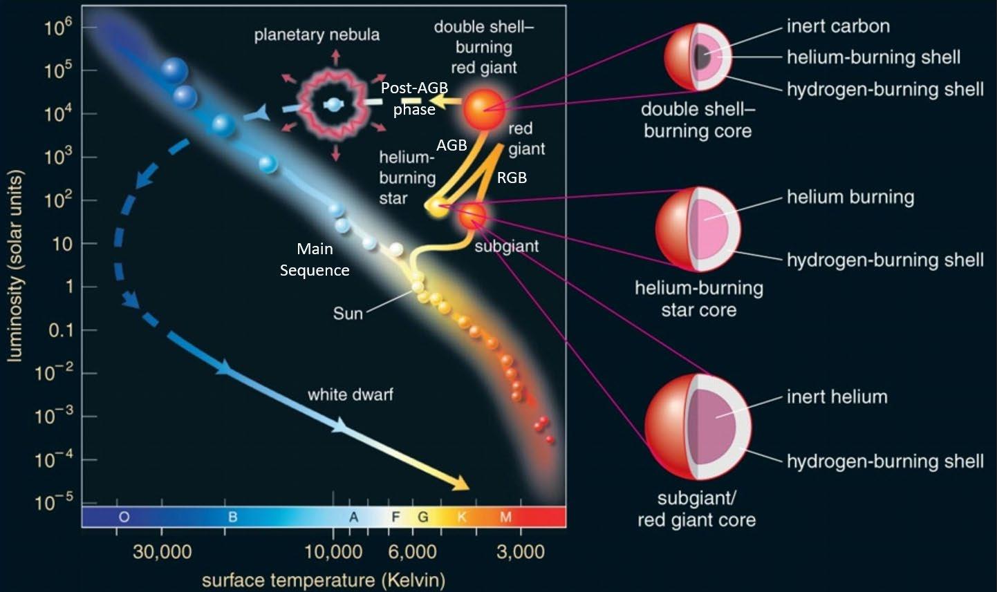
Figure 1. Hertzsprung-Russell diagram (H-R diagram) with an evolutionary track of a Sunlike star. The diagram plots a star’s luminosity against its surface temperature and is an extremely useful tool in astronomy to characterise a star’s properties. Note that neither time nor position in space is an axis within this diagram, so as a star evolves along an evolutionary track, it is not physically travelling anywhere, nor is the rate at which it is progressing along the track constant.

Credit: Adapted from Pearson Education 2004

1.1.2 Post-Asymptotic Giant Branch Stars

Evolutionary theory predicts that lowintermediate mass (0.6 M⊙ to 8 M⊙) post- AGB stars form in the transition between the AGB and a PN phases (see Figure 1). They appear as very luminous red giant stars with unique characteristics, having ejected their outer layers to reveal the star’s inner core for an astronomically short time period of 103 − 104 years 3 (van Winckel 2003). This inner core is composed of largely inert carbon and oxygen enriched with heavy elements formed from the s-process nucleosynthesis reactions. They exhibit a unique Spectral Energy Distribution (SED) which is characterised by two distinct curves, one in the shorter wavelengths generated by the inner star itself and the curve in the longer wavelengths due to the cooler shell of dust surrounding the star.

1.1.3. Binary Post-Asymptotic Giant Branch Stars

In a binary system, as one of the stars evolves and expands, material from one star can spill towards its partner, forming an accretion disk, also termed a transition disk 4 (Strom et al. 1989; Calvet et al. 2002, 2005; Kluska et al. 2022). These transition disks exhibit very similar properties to the protoplanetary disk around young stars(de Ruyter et al. 2006) described in Section 1.1.2, displaying potential to form second generation planets (Ertel et al. 2019). Post-AGB stars in a binary system (with a main sequence partner) also exhibit a characteristic depletion of refractory elements 5, not due to nucleosynthetic processes (Maas et al. 2003; Oomen et al. 2019), but rather, due to the rapid early condensation of these refractory elements as the post-AGB star expels its outer gaseous shells into the dusty disks, which are then blown away by radiation pressure whilst the volatile gaseous elements remain to be re-accreted into the post-AGB star.

In the spectral energy distribution (Figure 3), two blackbody curves are also similarly present 6 compared to the single post-AGB SED. However, this secondary curve is noticeably different from that of a single post-AGB star, appearing as a less distinct infrared excess.

Figure 2. Adapted from van Aarle et al. (2011). The spectral energy distribution for HD 56126, a carbon-rich single postAGB star, in the infrared region. The black curve represents the core star and the red curve represents the secondary blackbody spectrum due to the ejected dust shell.

3 comparatively, main sequence stars like the Sun can survive for 10^6 − 10^9 years

4 as they can be thought to be transitioning between full dusty disks and gas-less debris disks

5 elements that have relatively higher condensation temperatures, such as titanium

6 a curve within the shorter wavelengths is the core star’s blackbody distribution, and a curve in the longer wavelengths represents the scattering of light in the dusty transition disk, again shifted due to the dust’s temperature being cooler than the star itself.

Figure 3. Adapted from Kluska et al. (2022). The spectral energy distribution for IRAS19291+2149, a post-AGB binary, in the infrared region. The red is the best fit photospheric model for the core star, and the blue represents the Spitzer spectrum, highlighting the secondary blackbody spectrum due to the transition disk.

1.1.4. Target Sample

Binary post-AGB stars are potential sites of second generation planet formation so the sample from Kluska et al. (2022) was chosen as our target. This sample contains a list of all galactic post-AGB binaries characterised by their photometric properties by comparing the intensities of different wavelengths of emitted light (photometric bands) to identify larger scale properties such as stellar temperature, and disk structures by comparing the two unique blackbody curves within the SED (e.g. Figure 3); these disk structures within each category is displayed in Figure 4.

The Two Micron All-Sky Survey (2MASS) provided photometry in the near-IR wavelengths (conducted by various ground-based observatories) (Skrutskie et al. 2006), and the WISE surveys (conducted by the Wide-field Infrared Survey Explorer spacecraft) (Wright et al. 2010) provided mid- to far-infrared photometric data. Extremely highresolution spectra to provide chemical and kinematic information for target stars were generated by the APOGEE surveys (Apache Point Observatory Galactic Evolution Experiment) (Majewski et al. 2017) that characterised over half a million stars through near-infrared observation by measuring the intensity of certain spectral lines to determine chemical abundance; this is commonly notated as the logarithmic ratio of the desired element and hydrogen or iron compared to the Sun (i.e. [X/H] = log_10(NX/NH)_star-log_10(NX/NH)_Sun , where N denotes no. of particles and X denotes the element studied). A notable ratio is [Fe/H], known as metallicity, and is used as a measure of the abundance of elements heavier than helium (note all elements heavier than hydrogen and helium are termed a ‘metal’ within astronomy) 7

7 Other properties such as temperature and surface gravity are modelled via methods such as the Boltzmann excitation equation and Saha ionisation equation respectively, but is outside of the scope of this work.

Figure 4. Theorised scenarios for each category

(Kluska et al. 2022) .

1.1.5. Planet Metallicity Correlation

A Planet-Metallicity Correlation (PMC) has been found in many spectroscopic surveys, first recognised in exoplanet searches (Gonzalez 1997), which has lead to more detailed, larger scale investigations of this trend, producing a well-established correlation between planetary architecture and metallicity: higher metallicities of the host star correlated with increased planet formation. This is due to how the star’s chemistry is reflective of its homogeneous protostellar environment (Spina et al. 2021) - planets largely accrete from the heavier elements (metals) rather than hydrogen and helium.

Wilson et al. (2022) also expanded this work to the Kepler spectroscopic surveys (the Kepler space telescope targeted most G-type stars on/near the main sequence, see Figure 1) and found that a general increase in elemental abundance (C, Mg, Al, Si, S, K, Ca, Mn, Fe, and Ni) was correlated with an increase in planet occurrence, particularly larger planets with wider orbits. This was accomplished by assembling (from the Kepler survey) a sample of planet-containing stars and a control sample of stars chosen with properties (e.g. temperature, mass, photometric magnitudes) that reflect the bulk properties of the Kepler survey sample.

2. SCIENTIFIC FOCUS

Data from a variety of surveys (described in Section 1.1.4) is utilised to construct a comprehensive profile of transition disk properties, including the temperature, metallicity, and chemical abundance, of post-AGB binaries to extend a study by Wilson et al. (2022) which identified chemical anomalies in the composition of planet-containing stars from the Kepler survey that targeted younger, main sequence stars.

Thus, the scientific research question is: Do planet hosting Post-AGB binaries show trends between stellar properties and second generation planet formation that are valid proxies for planet identification?

3. METHODOLOGY

3.1. Data Collection

This study applied data from very recent papers (Kluska et al. 2022; Wilson et al. 2022) to search for planet-containing post-AGB binaries. I attempted to characterise stellar properties through stellar chemistry and other photometric properties by comparing trends found within this paper with the properties characterised by their SEDs by (Kluska et al. 2022). The target sample (Table 1) is a thorough list of post-AGB binaries that exhibit transition disks - the focus of this study. The chemical abundances for the elements studied by Wilson et al. (2022) (C, Mg, Al, Si, S, K, Ca, Mn, Fe, and Ni) expressed as [X/H] or [X/Fe]) were obtained by mining data from relevant abundance studies listed in Kluska et al. (2022). These elements allowed for a more direct cross-correlation comparisons and were also most commonly present within all the abundance studies (i.e. abundance studies did not always provide chemical abundances for every element). The respective temperature models and their stellar abundances models for each star were compiled into a single large spreadsheet. The categorisation by Kluska et al. (2022) was extended to include an additional category, ‘Cat. 3p’, to isolate the planet-containing stars in Cat. 3. Overall, these categories range from 0 to 4, with Cat. 2 and Cat. 3p’s transition disks exhibiting properties that are indicative of planet presence.

3.1.1. Cleansing

A significant amount of data cleansing was not required as the target sample was very definitive in containing all galactic post-AGB binaries. Stars where abundance values could not be found (i.e. the references did not lead to full abundance studies and no abundance data could be found) were omitted from the sample. This removed 25 stars from the original sample of 85, leaving 60 stars - this should still be noted to be a significant, large sample of post-AGB stars due to their rarity from their extremely short lifespans detailed in Section 1.1.1, so should still generate valid and significant results.

3.2. Data Processing

All abundances were converted to the abundance ratio of [X/Fe] using the formula [X/Fe] = [X/H] + [Fe/H] (noting that [Fe/H] is metallicity, which was one of the attributes collated by Kluska et al. (2022) within his star sample).

A Python program utilising Matplotlib was developed to produce various plots to process the data for analysis, with a unique marker used to denote each category of transition disk type across all plots:

• Abundance ratio of each element was plotted against effective temperature (stellar surface temperature), with a colourmap applied to show metallicity. Median lines were added, similarly to Wilson et al. (2022), to display potential trends between abundance and temperature which would invalidate trends observed in other graphs as a result of this spurious correlation; ideally, the crosses, representing the medians with bins of 500K, should remain close to the median without any significant correlation. Standard deviation intervals of 0.5σ, 1σ, and 2σ of the entire sample are also represented with grey lines to display the spread of data.

• Metallicity [Fe/H] was plotted against effective temperature. Medians for the planet-containing sample and the entire star sample was also plotted to allow for comparison between the two populations. Standard deviation intervals of 0.5σ, 1σ, and 2σ of the entire sample are also represented with grey lines to display the spread of data.

• Metallicity [Fe/H] was plotted against the orbital period of the binary system (note: this is not orbital period of potential planets). Medians for the planet-containing sample and the star sample was also plotted to allow for comparison between the two populations. Standard deviation intervals of 0.5σ, 1σ, and 2σ of the entire sample are also represented with grey lines to display the spread of data.

• Abundance ratio of each element was plotted against metallicity [Fe/H] with a linear regression model fitted to the planet-containing sample (green) and to the star sample (black). Standard deviation intervals of 0.5σ, 1σ, and 2σ of the entire sample are also represented with grey lines to display the spread of data.

• Abundance ratio of each element was plotted against metallicity [Fe/H], with the respective planet and control medians of the Kepler sample from Wilson et al. (2022).

This methodology has provided a comprehensive overview of the relationships between many different stellar properties to most effectively display differences within planetcontaining sample. Additionally, negligible risks and safety issues were present in this project due to its digital nature - all astrophysical data was obtainable from online databases and literature.

4. RESULTS

The graphs and plots outlined within Section 3.2 are displayed in the following figures:

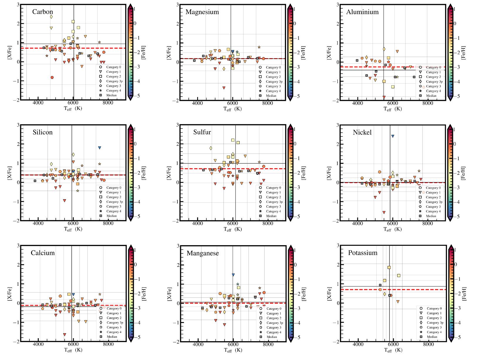
Figure 5. Abundance ratio vs effective temperature with a colourmap of metallicity. The horizontal red dashed lines represents the median of the sample. The solid black vertical and horizontal lines indicate the means of effective temperature and abundance ratio respectively. The white crosses represent the medians of bins of 500K. The grey grid represents standard deviation intervals of 0.5σ, 1σ, and 2σ for each axis.

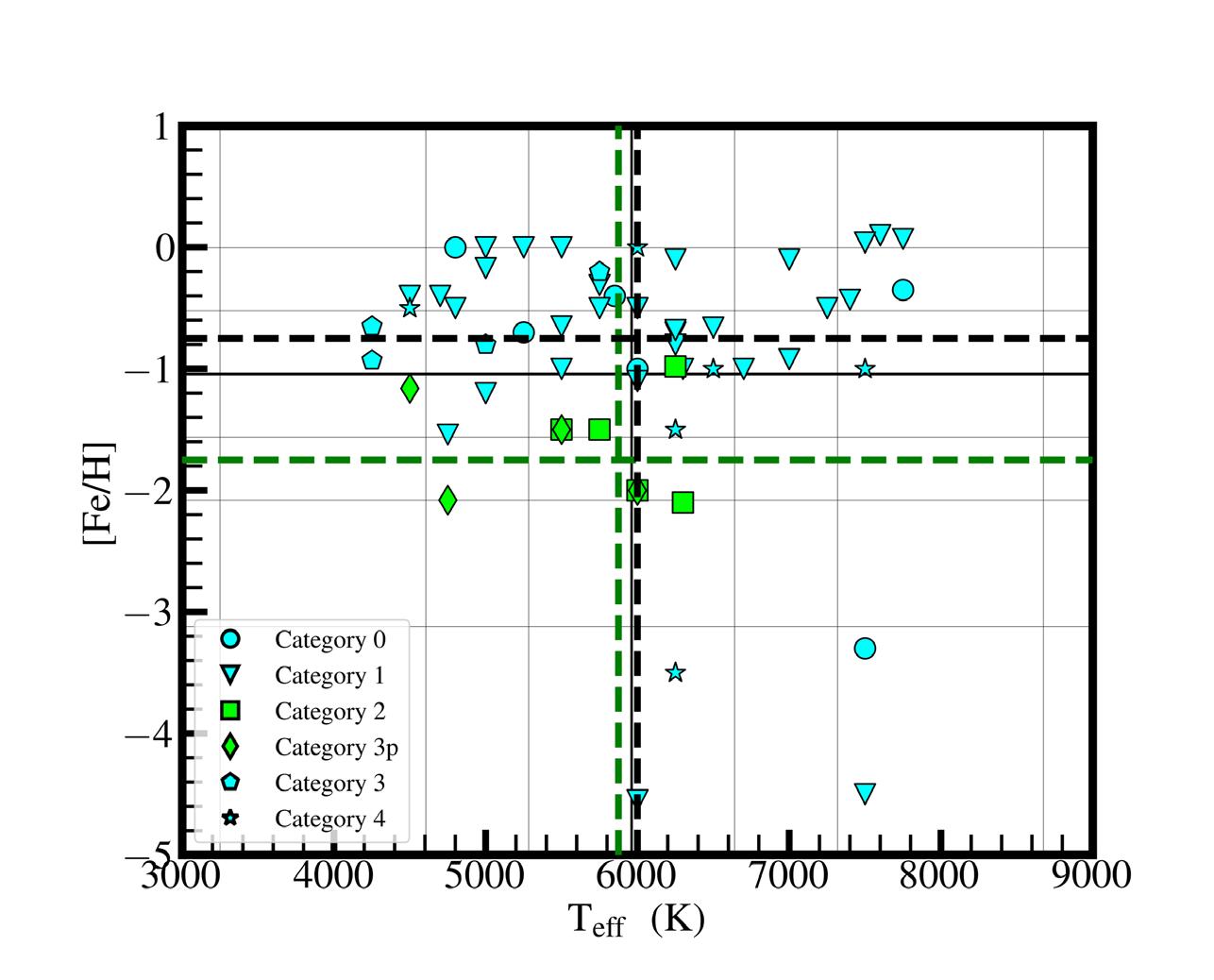
Figure 6. Metallicity vs effective temperature. Lime represents the planet-containing sample, cyan represents the non-planet-containing sample. The green dashed horizontal line indicates the median of metallicity of the planet-containing sample. The green dashed vertical line represents the median temperature of the planet-containing sample. The black dashed horizontal line indicates the median of metallicity of the entire target sample. The black dashed vertical line represents the median temperature of the entire target sample. The solid black vertical and horizontal lines indicate the means of effective temperature and metallicity respectively of the entire target sample. The grey grid represents standard deviation intervals of 0.5σ, 1σ, and 2σ for each axis.

Figure 7. Metallicity vs orbital period of the binary system. Lime represents the planetcontaining sample, cyan represents the non-planet-containing sample. The green dashed vertical and horizontal lines represents the median values of orbital period and metallicity respectively for the planet-containing sample. The black dashed vertical and horizontal lines represents the median values of orbital period and metallicity respectively of the entire target sample. The solid black vertical and horizontal lines indicate the means of orbital period and metallicity respectively. The grey grid represents standard deviation intervals of 0.5σ, 1σ, and 2σ for each axis.

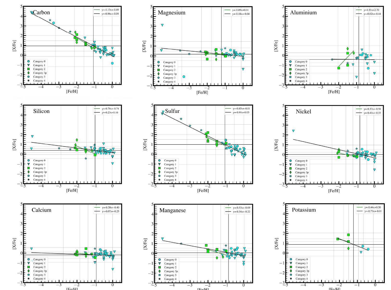
Figure 8. Plots of abundance vs metallicity. Lime represents the planet-containing sample, cyan represents the non-planet-containing sample. Regression lines are in green and black representing the planet-containing sample and entire target sample respectively. The solid black vertical and horizontal lines indicate the means of metallicity and abundance ratio respectively. The grey grid represents standard deviation intervals of 0.5σ, 1σ, and 2σ for each axis. Note the strongest regression lines for the entire target sample have Pearson’s correlation coefficients and p-values of: r_carbon=-0.96, p_carbon=2.3×10^-31; r_sulfur=-0.95, p_sulfur=2.6×10^-26; r_silicon=-0.53, p_silicon=2.9×10-5; r_nickel=-0.67, p_nickel=1.1×10-7.

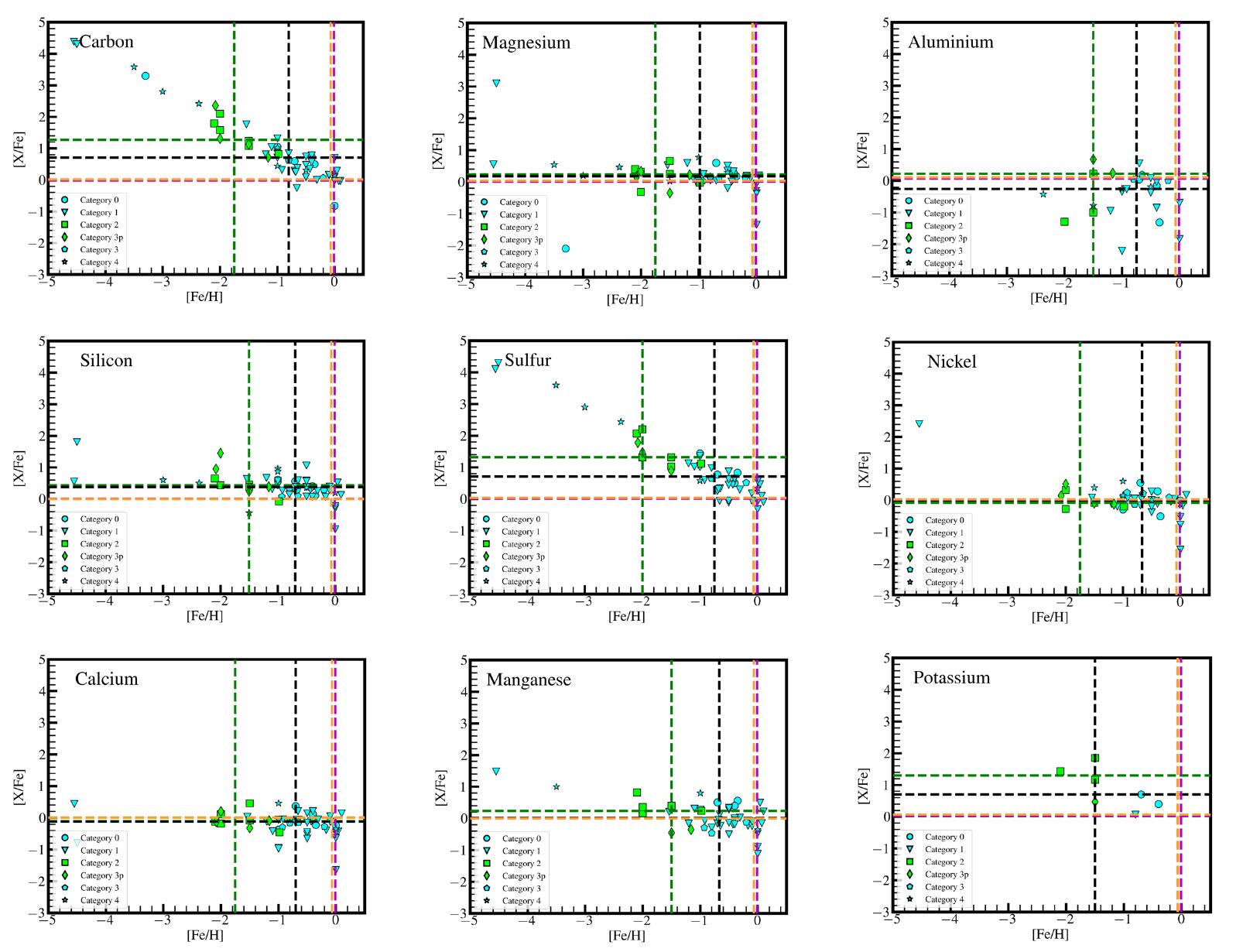
Figure 9. Plots of abundance vs metallicity. Lime represents the planet-containing sample, cyan represents the non-planet-containing sample. The green dashed vertical and horizontal lines represent the median values of metallicity and abundance ratio for the planet-containing sample. The black dashed vertical and horizontal lines represent the median values of metallicity and abundance ratio for the star sample. The red and purple dashed lines similarly represent the medians from Wilson et al. (2022) (also see Figure 10); purple is the planet-containing sample, tan is the control sample (refer to Section 1.1.5) .

5. DISCUSSION

5.1. Overview

5.1.1. Temperature Relations

Figure 5 displays chemical abundance against temperature with a colourmap displaying metallicity to show potential unwanted trends between temperature and chemical abundance which would lead to spurious correlations within other variables in the following graphs. PostAGB stars can have a large range in temperature depending on their age, so should not display any particular correlations between these properties:

• The magnesium, silicon, sulfur, nickel, calcium bin medians (the crosses) largely lie very close to this desired range.

• Even though the carbon, aluminum, and manganese bin medians do not all lie close to the desired median range, they effectively display no correlation between chemical abundance and temperature.

• The data sample available for potassium is much smaller than the other elements due to a lack of measurement from most abundance analyses (only 7 data points).

Thus, all chemical elements with the exception of potassium are valid for analysis 8; they have sufficiently large sample sizes which display no trends between temperature and chemical abundance. It is also noted that the planet-containing sample (Category 2 and Category 3p) has elevated chemical abundances for the α-elements carbon, silicon, sulfur, manganese, consistently lying above the median, elements that arise from similar nucleosynthetic origins of helium fusion (alpha process).

Within Figure 6, there is little offset in temperature between the medians of the planet-containing and population samples (125K) and the data displays little correlation with a Pearson’s correlation coefficient r = -0.14 (note it is slightly skewed by the extreme low metallicity stars, see Section 5.2) which is consistent with Figure 5 and general astronomical literature that no correlation between temperature and chemical properties should be present in post-AGB stars (Wilson et al. 2022).

5.1.2. Orbital Period Relations

An offset to longer stellar orbital periods and lower metallicities is present in the medians of the planet-containing stars compared against the entire sample median is evident within Figure 7, disagreeing with the PMC that higher metallicity stars are more likely to form planets (Osborn & Bayliss 2020). This reveals the need for new planetary formation models as the PMC only models 1st-generation planet formation; the materials that form 2nd-generation planets within these post-AGB binaries arise from drastically different origins: it is the metal-rich refractory dust expelled by the post-AGB star that forms planets rather than a homogeneous protostellar dust cloud, potentially indicating that planet forming post-AGB stars should be even more depleted in metals as these have left into the disk, which is supported by this data. The exact mechanism behind the offset to longer orbital periods is also unknown, with further researched needed.

5.1.3. Abundance Relations

Strong statistically significant correlations are present in Figure 8 between abundance and metallicity, particularly in the α-elements of carbon, sulfur, and silicon (r_carbon=-0.96, p_carbon=2.3×10^-31; r_sulfur=-0.95, p_sulfur=2.6×10^-26; r_silicon=-0.53, p_silicon=2.9×10-5; r_nickel=-0.67, p_nickel=1.1×10-7). This result is not present in the Wilson et al. (2022) study of the Kepler stars (see their results in Figure 10, consistent with the aforementioned theory because the younger, main sequence Kepler stars would not have undergone shell ejection processes associated with the post-AGB phase.

Furthermore, despite the slight lack of independence between the variables (i.e. an increase in carbon should result in an increase in metallicity due to the definition of ‘metals’ as elements heavier than helium - and carbon is one such element that is heavier than helium), this relationship also contradicts this proposition, also indicating further research is required to uncover the exact mechanism behind this trend.

In Figure 9, the medians of the planetcontaining stars are noticeably offset from the sample medians with much lower metallicities, consistent with Figure 7 that 2nd-generation planet formation is associated with extra depleted stars. Additionally, if the extreme depleted stars ([Fe/H] ≤ 3) are disregarded, the planetcontaining stars lie clearly within a separate ‘cluster’ in Figure 9 at much lower metallicities. This offset is not consistent with the results of Wilson et al. (2022), where planet-containing stars have slightly lower metallicities, indicating differences in the process of planet formation that will require further modelling and study.

5.2. Extreme Stars

There are a number of ‘extreme’ stars (HD 52961, HR 4049, CC Lyr, HD 44179, HD 137569) with extremely low metallicities ([Fe/H] ≤ 3). These stars are found to show no obvious links with transition disk formation, suggesting an unknown depletion mechanism is present within the stellar system, and it is unknown if this depletion mechanism is the same as the rest of the target sample population (Kluska et al. 2022). This factor has motivated the use of medians rather than means to provide a more accurate depiction of the data’s central tendency.

5.3. Limitations

Due to the exploratory nature of this study, more information is required on the dust formation and processing within the disks themselves. Current literature does not fully understand the physics behind the planet formation process within these transition disks such as inhomogeneities within disk material, nor the morphology and true structure of the transitions disks - we only have photospheric parameters from which we attempt to infer properties.

Omitting the stars for which abundance could not be found should not introduce bias, as this was likely due to random chance that the omitted stars did not have accessible chemical abundances. This work has aimed to avoid spurious correlations, such as temperatureabundance relations, but notes many confounding variables that may be present such as relative trends with stellar age, and stellar mass which could not be accounted for due to a lack of data.

5.4. Future Scope

As this project is the first study analysing the chemical composition of different categories of binary post-AGB stars with a special focus on stars with transition disks, significantly more study into the sample is needed, such as developing and comparing these results with stellar models to fully understand the mechanism behind these trends and address the gaps within our knowledge, such as the many peculiar metallicity and abundance relationships. The population of extreme stars also warrants further study into their depletion mechanisms, i.e. what has caused them to become so extremely metal poor.

Another immediate continuation of this work is to extend the sample of analysed post-AGB binaries to increase the statistical significance of results by extending this sample to extra-galactic stars, such as the Magellanic Clouds. In addition, explorations on the applicability of the patterns found within this study to other stars, such as single post-AGB systems, can be conducted to produce a more holistic set of parameters defining planet occurrence via stars’ chemical properties.

6. CONCLUSION

This project has characterised how the properties of 2nd-generation planetcontaining post-AGB binaries differ from the galactic population; they have higher orbital periods, and higher median elemental abundances (with particular elevations in the abundances of αelements such as carbon, silicon, sulfur, and manganese) but with lower metallicities. The post-AGB sample disobeys the PMC that characterises 1stgeneration planet forming stars likely due to the very different mechanisms behind disk and planet formation but further research is needed to determine the exact processes involved. The comparison of this study’s results with the Kepler stars in Wilson et al. (2022) have also reflected this theory, where the postAGB sample had much lower metallicities whilst the planet-containing Kepler sample of main sequence stars had higher metallicities that followed the PMC.

ACKNOWLEDGEMENTS

I would like to thank my science extension teacher, Dr Dennis, for her tireless support of this project, by providing constant guidance, putting me in touch with my Macquarie University mentor, Dr Kamath, and help in proofreading and editing this report.

I would also like to thank Dr Kamath and her group of PhD students for teaching me so much about astronomy and post- AGB stars, and her patience in guiding me until its completion, allowing me to gain the wide range of astrophysical knowledge and skills required for this project, including how to utilise the NASA ADS system to effectively find literature, and the use of LATEX to typeset my report, not to mention her assistance in also proofreading and editing this report to point me in the right direction in this project.

I would also like to extend my thanks to my friends, Michael Chen and Kerui Yang, who have supported me in proofreading my work and helped troubleshoot issues when things went wrong within my Python scripts and project.

REFERENCES

Calvet, N., D’Alessio, P., Hartmann, L., et al. 2002, ApJ, 568, 1008, doi: 10.1086/339061

Calvet, N., D’Alessio, P., Watson, D. M., et al. 2005, ApJL, 630, L185, doi: 10.1086/491652

de Ruyter, S., van Winckel, H., Maas, T., et al. 2006, A&A, 448, 641, doi: 10.1051/0004-6361:20054062

Ertel, S., Kamath, D., Hillen, M., et al. 2019, AJ, 157, 110, doi: 10.3847/15383881/aafe04

Gezer, I., Van Winckel, H., Bozkurt, Z., et al. 2015, MNRAS, 453, 133, doi: 10.1093/mnras/stv1627

Gezer, I., Van Winckel, H., Manick, R., & Kamath, D. 2019, MNRAS, 488, 4033, doi: 10.1093/mnras/stz1967

Giridhar, S., & Arellano Ferro, A. 2005, A&A, 443, 297, doi: 10.1051/00046361:20041495

Giridhar, S., Molina, R., Arellano Ferro, A., & Selvakumar, G. 2010, MNRAS, 406, 290, doi: 10.1111/j.13652966.2010.16696.x

Gonzalez, G. 1997, MNRAS, 285, 403, doi: 10.1093/mnras/285.2.403

Gorlova, N., Van Winckel, H., Gielen, C., et al. 2012, A&A, 542, A27, doi: 10.1051/0004-6361/201118727

Gorlova, N., Van Winckel, H., Ikonnikova, N.P., et al. 2015, MNRAS, 451, 2462, doi: 10.1093/mnras/stv1111

Kamath, D. 2020, Journal of Astrophysics and Astronomy, 41, 42, doi: 10.1007/s12036-020-09665-4

Klochkova, V. G., & Panchuk, V. E. 1996, Bulletin of the Special Astrophysics Observatory, 41, 5

Kluska, J., Van Winckel, H., Copp´ee, Q., et al. 2022, A&A, 658, A36, doi: 10.1051/0004-6361/202141690

Maas, T., Giridhar, S., & Lambert, D. L. 2007, ApJ, 666, 378, doi: 10.1086/520081

Maas, T., Van Winckel, H., Lloyd Evans, T., et al. 2003, A&A, 405, 271, doi: 10.1051/0004-6361:20030613

Majewski, S. R., Schiavon, R. P., Frinchaboy, P. M., et al. 2017, AJ, 154, 94, doi: 10.3847/1538-3881/aa784d

Manick, R., Miszalski, B., Kamath, D., et al. 2021, MNRAS, 508, 2226, doi: 10.1093/mnras/stab2428

Olofsson, H., Vlemmings, W. H. T., Maercker, M., et al. 2015, A&A, 576, L15, doi: 10.1051/0004-6361/201526026

Oomen, G.-M., Van Winckel, H., Pols, O., & Nelemans, G. 2019, A&A, 629, A49, doi: 10.1051/0004-6361/201935853

Oomen, G.-M., Van Winckel, H., Pols, O., et al. 2018, A&A, 620, A85, doi: 10.1051/0004-6361/201833816

Osborn, A., & Bayliss, D. 2020, MNRAS, 491, 4481, doi: 10.1093/mnras/stz3207

Skrutskie, M. F., Cutri, R. M., Stiening, R., et al. 2006, AJ, 131, 1163, doi: 10.1086/498708

Sloan, G. C., Kraemer, K. E., Wood, P. R., et al. 2008, ApJ, 686, 1056, doi: 10.1086/591437

Spina, L., Sharma, P., Mel´endez, J., et al. 2021, Nature Astronomy, 5, 1163, doi: 10.1038/s41550-021-01451-8

Strom, K. M., Strom, S. E., Edwards, S., Cabrit, S., & Skrutskie, M. F. 1989, AJ, 97, 1451, doi: 10.1086/115085

van Aarle, E., van Winckel, H., Lloyd Evans, T., et al. 2011, A&A, 530, A90, doi: 10.1051/0004-6361/201015834

van Winckel, H. 2003, ARA&A, 41, 391, doi: 10.1146/annurev.astro.41.071601.17001 8

Wilson, R. F., Ca˜nas, C. I., Majewski, S. R., et al. 2022, AJ, 163, 128, doi: 10.3847/1538-3881/ac3a06

Wright, E. L., Eisenhardt, P. R. M., Mainzer, A. K., et al. 2010, AJ, 140, 1868, doi: 10.1088/0004-6256/140/6/1868

APPENDIX

A. FULL TARGET SAMPLE PROPERTIES

B. FULL TARGET SAMPLE ABUNDANCES

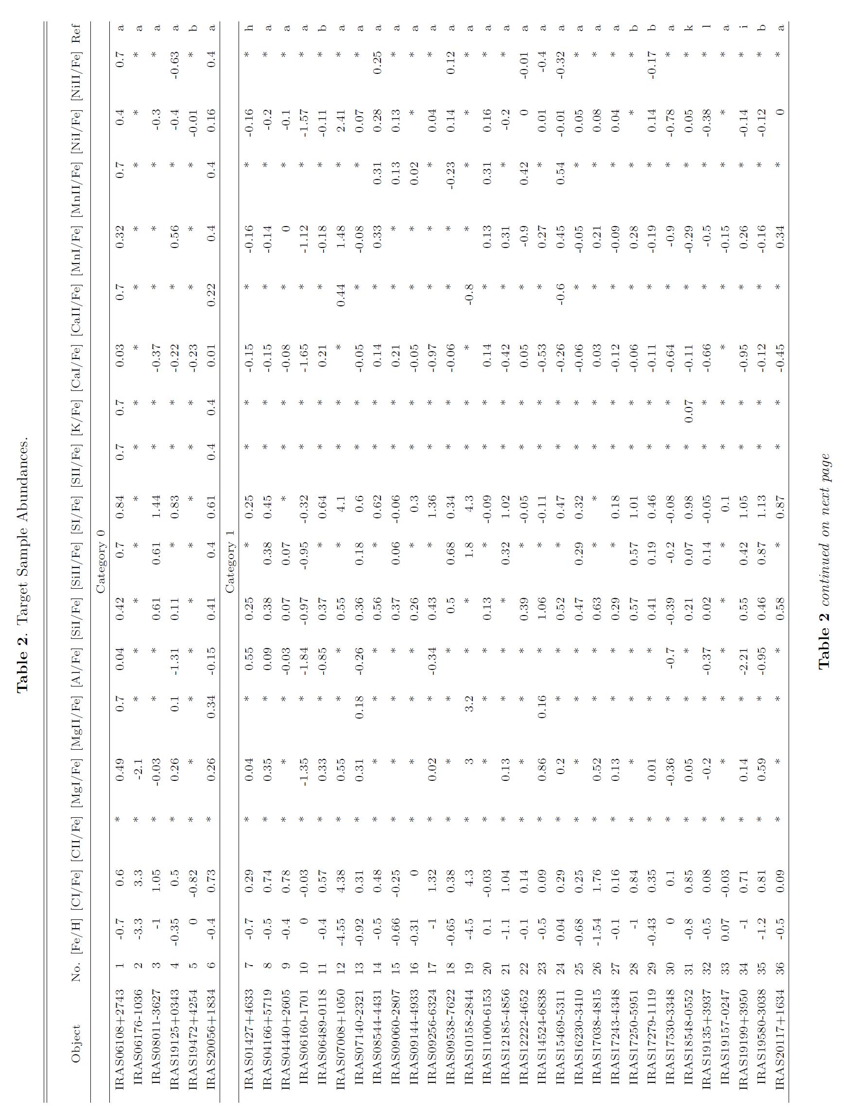
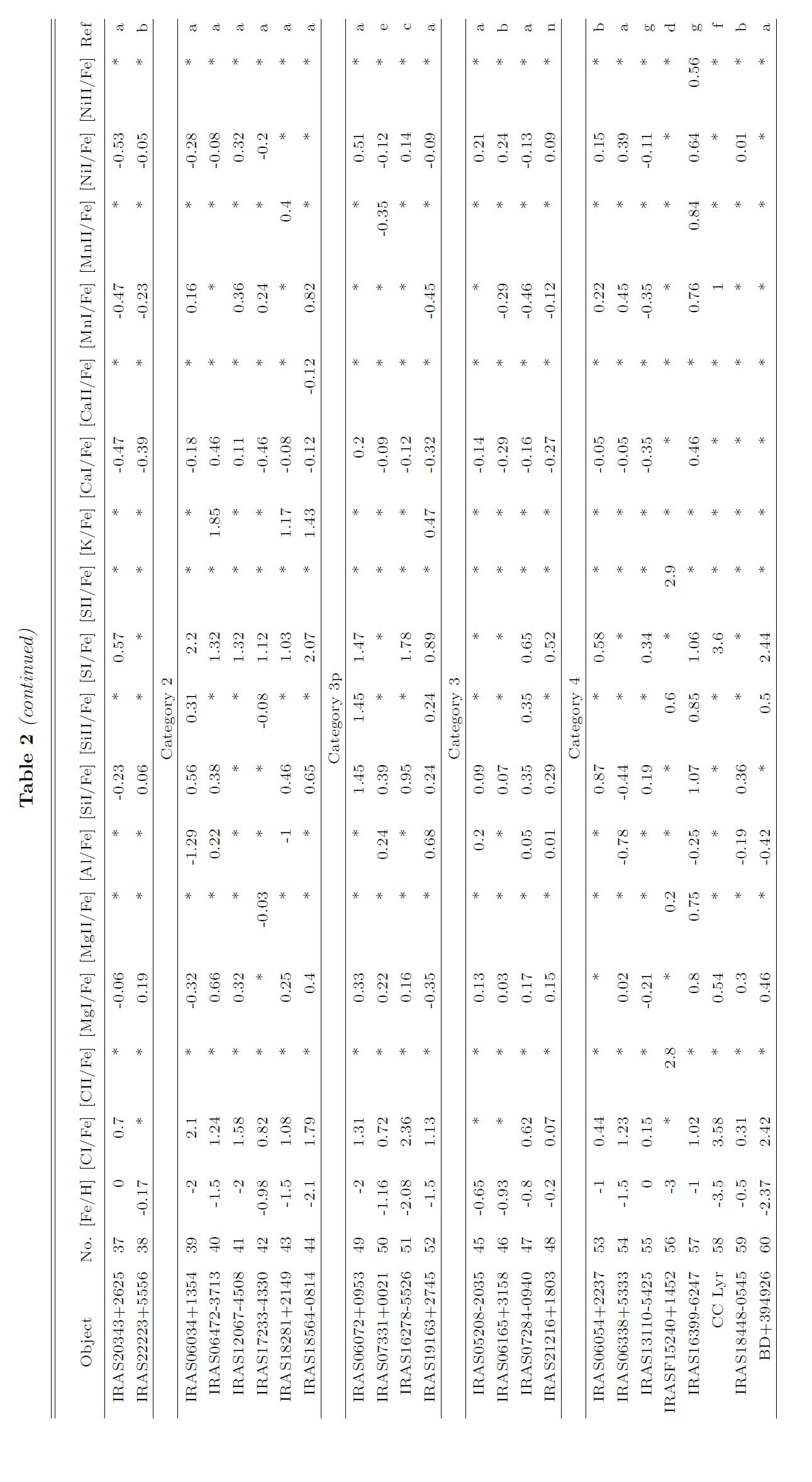
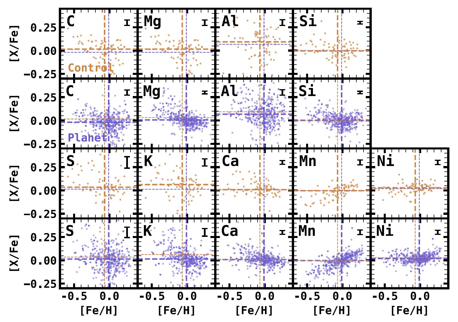
Figure 10. Adapted results from Wilson et al. (2022). Chemical abundances for the planet host (purple) and control (tan) samples. The chemical abundance displayed is shown in the upper left corner of each panel. The median error (±1σ) for each abundance is shown by the black error bar in the top right corner of each panel, and the dashed lines indicate the median abundances for the planet host sample (purple) and the control sample (tan).