The Journal of l\l.k -----~§yt Science Extension Research NSW Department of Education Volume 1, 2022
Image credit:
Cover - Megan Jeffers, Ulladulla High School

Inside cover - Keetan Southwell, St. Ives High School
NSW Department of Education
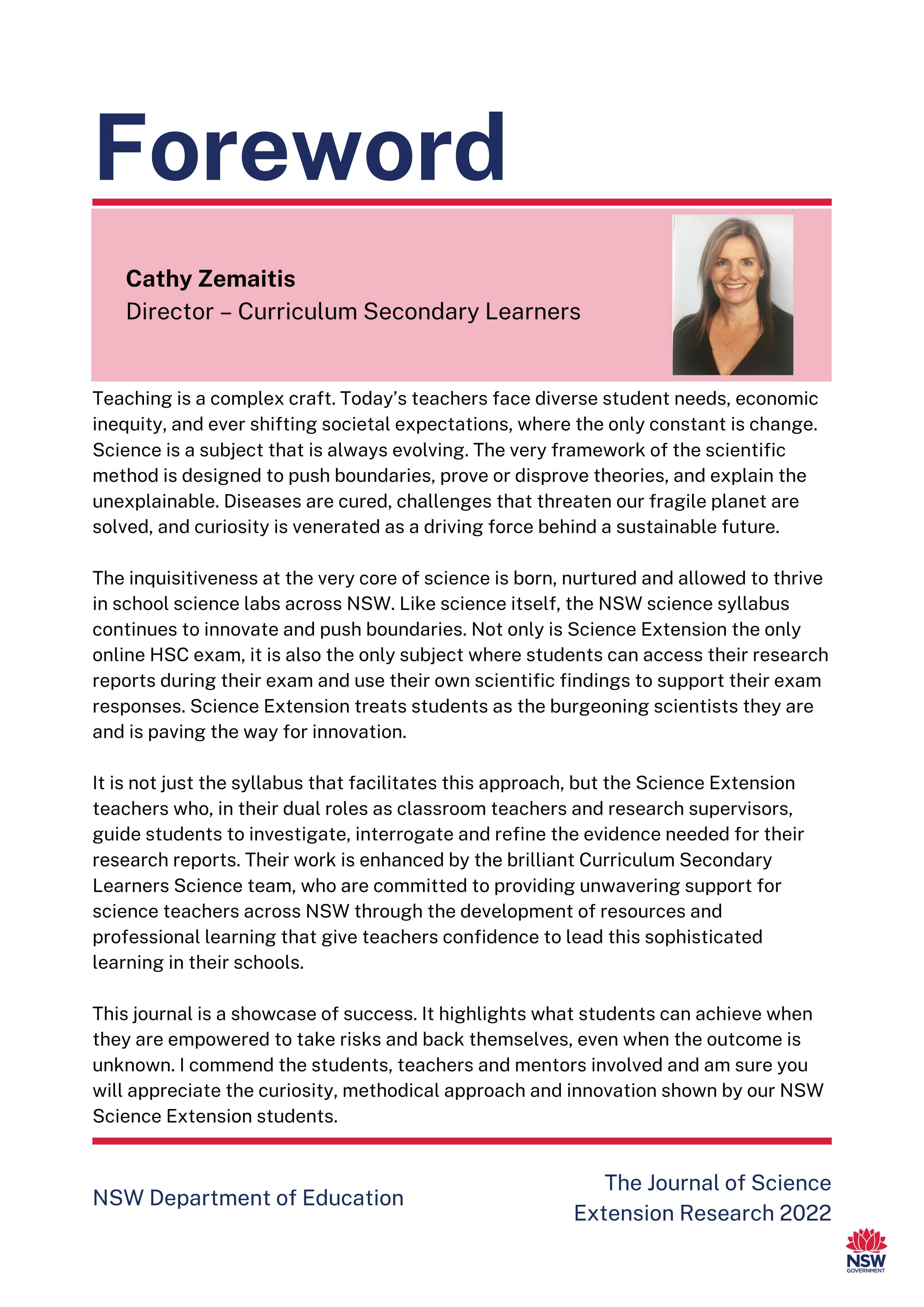
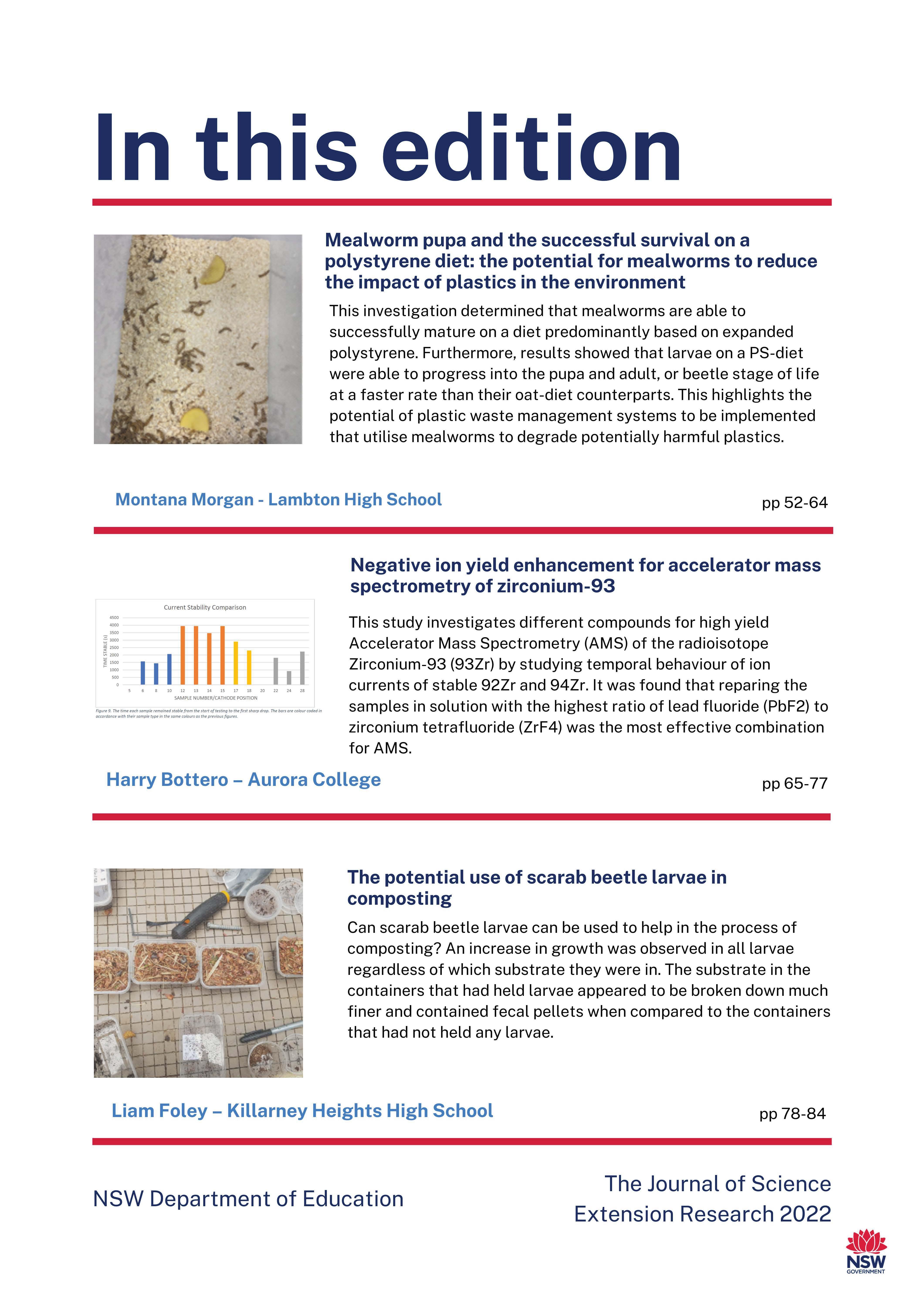
Image 1: Testing rig loaded with a test strip.

Table of Contents 4 ···················· Forewords 7 Acknowledgments 8 ···················· Introduction 9 ···················· In this edition 12 ···················· Student reports The Journal of Science NSW Department of Education Extension Research 2022
Foreword
Cathy Zemaitis Director - Curriculum Secondary Learners
Teaching is a complex craft. Today's teachers face diverse student needs, economic inequity, and ever shifting societal expectations, where the only constant is change. Science is a subject that is always evolving. The very framework of the scientific method is designed to push boundaries, prove or disprove theories, and explain the unexplainable. Diseases are cured, challenges that threaten our fragile planet are solved, and curiosity is venerated as a driving force behind a sustainable future.
The inquisitiveness at the very core of science is born, nurtured and allowed to thrive in school science labs across NSW. Like science itself, the NSW science syllabus continues to innovate and push boundaries. Not only is Science Extension the only online HSC exam, it is also the only subject where students can access their research reports during their exam and use their own scientific findings to support their exam responses. Science Extension treats students as the burgeoning scientists they are and is paving the way for innovation.
It is not just the syllabus that facilitates this approach, but the Science Extension teachers who, in their dual roles as classroom teachers and research supervisors, guide students to investigate, interrogate and refine the evidence needed for their research reports. Their work is enhanced by the brilliant Curriculum Secondary Learners Science team, who are committed to providing unwavering support for science teachers across NSW through the development of resources and professional learning that give teachers confidence to lead this sophisticated learning in their schools.
This journal is a showcase of success. It highlights what students can achieve when they are empowered to take risks and back themselves, even when the outcome is unknown. I commend the students, teachers and mentors involved and am sure you will appreciate the curiosity, methodical approach and innovation shown by our NSW Science Extension students.
The Journal of Science
NSW Department of Education Extension Research 2022
Foreword
Kerry Sheehan, Inspector, Science NESA
The Science Extension syllabus, developed by New South Wales Education Standards Authority (NESA), allows our senior NSW science students to investigate issues and phenomena close to their hearts. Its intrinsically motivating, challenging and inherently exciting. The course allows students to go beyond the expected and to tangibly demonstrate excellence. The student research examples provided in this journal pay testament to this and to the students who have completed the course and who remain on our starship continuing, as Captain James T. Kirk explained, 'to go where no one has ever gone before'.
The NSW Department of Education has given me this opportunity to introduce this Science Extension journal. I will also take this opportunity to congratulate the Department staff who have embraced the course and have been instrumental in providing ongoing support to our NSW science students, their teachers, and the many academics and student mentors. For this I am grateful.
I have always had a love for science and have long understood that the scientific method is humankind's greatest tool. The application of the method enables our continued human adventure. The scientific method, when applied authentically, reveals to us the unknown. Scientific research changes our science fictions into our lived realities and allows us to decide our destiny.
The starship we inhabit is full of people working for the common good and striving to make our world a better place. What are the common characteristics of these people? I believe, they maintain a belief that things can and will be better, that problems are there to be solved and that learning provides them with the opportunity and wherewithal to go and do something about the things that are of concern.
As have all generations, our young people have significant issues to overcome. The examples in this journal of the skill and intellect of our young people shows that they are well able to re-write the future. Many of them, I believe, are destined to be our greatest problem solvers and household names. This journal demonstrates that our young are aware of many of the issues and opportunities confronting them. Within this journal they demonstrate, through their research, they have the tools to, 'seize the day' where opportunity knocks, and to fix the things, we are leaving them to fix. It is only through the application of the scientific method drawing on our bank of scientific knowledge that this will occur.
I commend this journal to you and wish all past, present and future Science Extension students Godspeed in their future quests upon Starship Earth
The Journal of Science NSW Department of Education Extension Research 2022
Foreword
Professor Hugh Durrant-Whyte, NSW Chief Scientist & Engineer

It's a pleasure to introduce the inaugural Journal of Science Extension Research, which showcases some of the incredible independent research being undertaken by students as part of the HSC Science Extension course.
Although not often thought of in this way, science is an artform requiring passion, creativity and freedom of ideas. That's what is so important about the Science Extension course - it allows students to pursue a line of research outside of the constraints of a curriculum. This is the kind of experience that bridges the gap between simply studying science and becoming a scientist
I am truly impressed by the calibre of work in this journal, which is a testament to the exceptional young scientific minds we have in NSW. I am hopeful that many of you will translate your interest in science into a science, technology, engineering or mathematics (STEM) career, as we need more STEM professionals to tackle our state's most pressing problems.
A STEM career provides almost endless opportunities - personally, it has allowed me to travel the world and be involved in exciting projects delivering real-world impact in areas including robotics, mining, and defence.
Promoting STEM careers is something I am passionate about. Indeed, encouraging the next generation of scientists to realise their potential is a focus of the Office of the NSW Chief Scientist & Engineer. We support many programs including the Science and Engineering Challenge, National Youth Science Forum and the Supporting Young Scientists Program, which I encourage students to explore.
I would like to thank the teachers who produced this journal for supporting and inspiring students to embrace their passion for science and pursue it as a career. Congratulations to those published - no doubt I may meet you down the track. I'm excited to see where your scientific journey takes you from here.
The Journal of Science
Extension Research 2022
NSW Department of Education
Acknowledgements
The Science 7-12 curriculum team acknowledges the incredible efforts of Science Extension teachers in inspiring, guiding and mentoring their students to complete their scientific research projects. Despite the novelty and innovativeness of the syllabus, those teachers spared no effort to nurture their students' scientific curiosity and engage them in conducting authentic scientific inquiry. As a result, their students have experienced new heights of academic and scientific achievements in their research Journeys.
We acknowledge the following teachers whose students' reports appear in this publication:
• Tim Smith, St. Ives High School
• Ann Hannah, Menai High School
• Sylvia Rudmann, Aurora College
• Joshua Westerway, Ulladulla High School

• Suzanne Wilson, Killarney Heights High School
• Kurt Nicholson, Lambton High School
Journal of Science Extension Research 2022
The

To all NSW Department of Education schools, we thank you for your sustained efforts to achieve excellence in science education.
NSW Department of Education
Introduction
The Science Extension course
The course enables students to engage in authentic scientific research. They experience the approaches used by professional scientists to construct explanations of natural phenomena. Students document their research experiences in a Research Portfolio and produce a Scientific Research Report that bears the hallmarks of scientific publications.
This scientific journal is a celebration of students' achievements in scientific research in the Science Extension course. It illustrates the depth and quality of scientific output that our inspired high school science students can produce when unfettered by content-driven investigations.
The Journal of Science NSW Department of Education Extension Research 2022
In this edition
In this inaugural edition, research reports from Science Extension students who completed the course in 2020 and 2021 are included. All reports are the work of students studying in NSW public schools. They have been supported by their teachers and schools, and in some cases, external mentors.
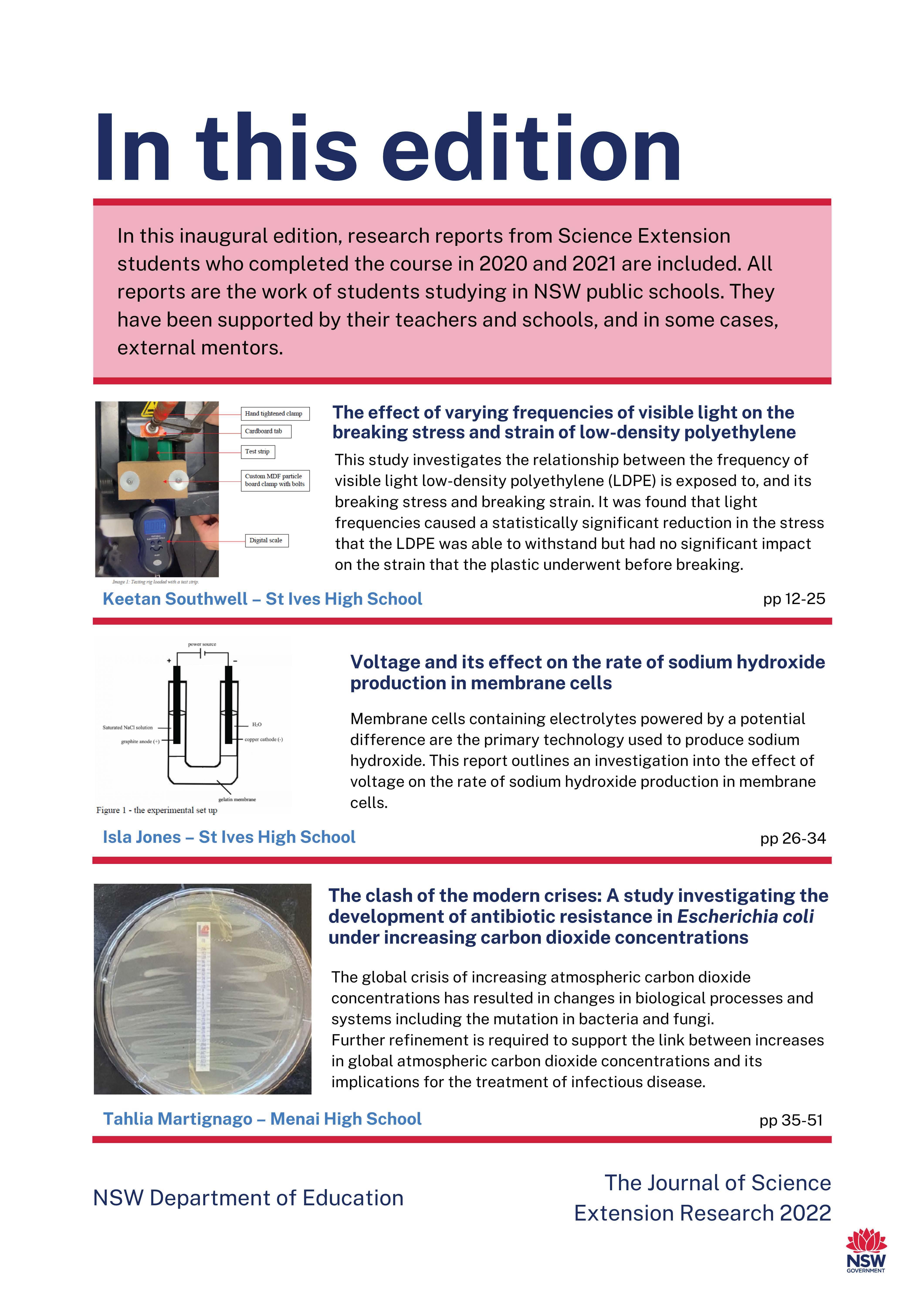
The effect of varying frequencies of visible light on the breaking stress and strain of low-density polyethylene
This study investigates the relationship between the frequency of visible light low-density polyethylene (LDPE) is exposed to, and its breaking stress and breaking strain. It was found that light frequencies caused a statistically significant reduction in the stress that the LDPE was able to withstand but had no significant impact on the strain that the plastic underwent before breaking.
Voltage and its effect on the rate of sodium hydroxide production in membrane cells
Membrane cells containing electrolytes powered by a potential difference are the primary technology used to produce sodium hydroxide. This report outlines an investigation into the effect of voltage on the rate of sodium hydroxide production in membrane cells.
The clash of the modern crises: A study investigating the development of antibiotic resistance in Escherichia coli under increasing carbon dioxide concentrations
The global crisis of increasing atmospheric carbon dioxide concentrations has resulted in changes in biological processes and systems including the mutation in bacteria and fungi. Further refinement is required to support the link between increases in global atmospheric carbon dioxide concentrations and its implications for the treatment of infectious disease.
School pp 35-51
Keetan Southwell - St Ives High School pp 12-25
"" eoppcrcalhodc(-) pphitcanode(+) ,clarin mcmbrmc F igme l - the expe rimental set up
Isla Jones - St Ives High School pp 26-34
Tahlia Martignago - Menai High
The Journal of Science NSW Department of Education Extension Research 2022
In this edition
Mealworm pupa and the successful survival on a polystyrene diet: the potential for mealworms to reduce the impact of plastics in the environment
This investigation determined that mealworms are able to successfully mature on a diet predominantly based on expanded polystyrene. Furthermore, results showed that larvae on a PS-diet were able to progress into the pupa and adult, or beetle stage of life at a faster rate than their oat-diet counterparts. This highlights the potential of plastic waste management systems to be implemented that utilise mealworms to degrade potentially harmful plastics.
52-64
Negative ion yield enhancement for accelerator mass spectrometry of zirconium-93
This study investigates different compounds for high yield Accelerator Mass Spectrometry (AMS) of the radioisotope Zirconium-93 (93Zr) by studying temporal behaviour of ion currents of stable 92Zr and 94Zr. It was found that reparing the samples in solution with the highest ratio of lead fluoride (PbF2) to zirconium tetrafluoride (ZrF4) was the most effective combination for AMS.
65-77
The potential use of scarab beetle larvae in composting
Can scarab beetle larvae can be used to help in the process of composting? An increase in growth was observed in all larvae regardless of which substrate they were in. The substrate in the containers that had held larvae appeared to be broken down much finer and contained fecal pellets when compared to the containers that had not held any larvae.
Montana Morgan - Lambton High School pp
current Stabili y Comparison I
"" o n, " ach ,a lo rcmo.-, d ,to!k '. ",,,. ,tort.oft<,M1 ,o 111 ·,t,no"' arop. 71>< OOr<a.< co!ourcod d,n ""'-"""'"°'"'""'''m,,,.., * """'Cf'"&l>'"''--n ,
I I IIIII I I I
Harry Bottero - Aurora College pp
The Journal of Science NSW Department of Education Extension Research 2022
Liam Foley - Killarney Heights High School pp 78-84
In this edition
Microplastic contamination of urban and bushland dominated beaches of the Shoalhaven
Microplastics in the marine environment represent a form of pollution of increasing concern. This investigation examined two beaches in the Shoalhaven for microplastic abundance. The results suggest that urban dominated beaches, as represented by Ulladulla Harbour, have a higher risk of microplastic occurrence.
Megan Jeffers - Ulladulla High School
pp 85-95
Succession of Diptera and Coleoptera taxa of plastic wrapped and unwrapped carcasses in coastal New South Wales
This study investigated if plastic wrapping of carcasses delay the insect succession in coastal New South Wales. Piglet carcasses were used and focus was placed on Coleoptera and Diptera taxa. Delays of wrapped carcasses were also observed on the other species recorded with a few notable exceptions. C. rufifacies and P. lacrymosa colonised the wrapped carcasses three and eleven days before the unwrapped.
Meirah Patterson - Ulladulla High School
Bugs on Drugs
pp 96-105
This study investigates the impact of caffeine and antihistimine on the conglobation behaviour of the Armadillidium Vulgare (pill bugs). Both drug classes impacted upon the conglobation behaviour of the pill bug which suggests that drugs polluting water sources in pill bug habitats could be placing stresses on the species and threaten their survival.
Sidney Breth Petersen - Killarney Heights High School
pp 106-115
)j
oa-,,aa.,_i 0 " I Oi,t,NaC..li.,.....id•<a....,..,......l<Mi,..olioiFigure S-Coleoptera and D ptera Succession
of Wrapped Carcasses
The Journal of Science NSW Department of Education Extension Research 2022
The effect of varying frequencies of visible light on the breaking stress and strain of low-density polyethylene
Keetan Southwell
St. Ives High School
The degradation of a polymer can be indirectly measured through the change in its breaking stress and strain before and after the degradative process. The purpose of this study is to investigate the relationship between the frequency of visible light low-density polyethylene (LDPE) is exposed to, and its breaking stress and breaking strain. LDPE test strips were exposed to three different frequencies of visible light. The stress-strain relationship of each test strip was then investigated to measure the effect that the light had on the plastic. It was found that light frequencies of 4.79*10¹⁴ Hz (red), 5.86*10¹⁴ Hz (green) and 6.43*10¹⁴ Hz (blue) caused a statistically significant reduction in the stress that the LDPE was able to withstand but had no significant impact on the strain that the plastic underwent before breaking when compared to a control group. This indicates that visible light can cause photodegradation.
1.LITERATURE REVIEW
Polymers are desired for their resistance to degradation under environmental pressures, such as temperature, acidity, and light. Polymers are also desirable for their mechanical properties, such as their strength and elasticity. Because of this durability, plastics accumulate in the environment (Ojeda 2013).
Polyethylene accounts for 37.2% of all plastic manufactured (PlasticsEurope 2018) and polyethylene, particularly LDPE is the main component in plastic bags (PlasticsEurope 2018). These two factors combined are why LDPE was chosen for this investigation over other polymers.
It is understood that ultraviolet light causes a reduction in the mechanical integrity of LDPE (Kelly & White 1996), however, an existing study relating visible
light frequency to degradation in stress and strain could not be found. Visible frequencies of light were shown to reduce the mechanical integrity of LDPE when catalysed by metal oxides (Venkataramana et al. 2020). There is no significant weight loss of LDPE under shorter-term exposure (128 h) to visible light (Liu et al. 2013), in agreeance with the degradation curve provided by Schnabel (2014), showing that the degradation rate of polymers was reduced significantly after 100 h of exposure to electromagnetic radiation.
The tensile strength and strain of LDPE has not been examined following the short-term exposure to visible light (128 hours) and so this is the chosen time for this investigation.
The purpose of this investigation is to analyse how different light frequencies of blue light (���� =6.43 ∗ 1014 Hz), red light
The Journal of Science Extension Research – Vol. 1, 2022 education.nsw.edu.au 12
(���� =4.79 ∗ 1014 Hz) and green light (���� = 5.86 ∗ 1014 Hz) change the breaking stress and breaking strain of the plastic under an exposure time of 128 hours. It is hypothesised that under exposure to visible light, all frequencies will cause a significant reduction in the breaking stress and strain of LDPE. The defined α for this investigation is 0.05.
There are several key structural differences between LDPE and other polyethylene (PE), variants. LDPE has shorter alkyl chained molecules with a greater number of branches compared to the longer chains of linear LDPE (LLDPE), or the even longer chains and reduced number of branches in highdensity PE (HDPE). (Khanam & AlMaadeed 2015). This gives LDPE a lower rigidity because of the more random packing of its polymer chains compared to HDPE (Khanam & AlMaadeed 2015)
Polymer degradation is a multi-step process in which a polymer undergoes a series of chemical changes. In photodegradation, the process is initiated by photons being absorbed into reactive areas of the polymer causing molecular excitement (Yousif & Haddad 2013) These more reactive groups are any functional groups that may be included in the polymer. These can include hydroperoxide groups, carbonyl groups, unsaturated carbon bonds or metal oxide imperfections in the polymer (Schnabel 2014). In theory, because polyethylene does not contain any of these active groups in its structure (CH2 CH2)n it should be stable, however, commercial LDPE such as the product used in this investigation has imperfections that occur in the manufacturing process (Rabek 1995). This allows it to be affected by
visible and ultraviolet light photons (Rabek 1995) During photodegradation, photons cause the radicalisation of certain parts of the polymer chain in which carbons lose their hydrogens (Yousif & Haddad, 2013). This free carbon radical is allowed to oxidise, forming a peroxide and then a hydroperoxide. With the input of more energy in the form of photons, the radicals and the hydroperoxide splits into a hydroxyl group and a C-O* radical, allowing for chain scission to occur (Yousif & Haddad, 2013). This causes the break in the polymer chain (Reusch 2015) and in the case of polyethylene, a dicarboxylic acid is formed (Gewert et al. 2018) Generally, the length of a radical that is released during the degradation can have an alkyl chain of a length between 8 and 12, and 14 and 20 carbons with octanedioic acid, decanedioic acid and tetradecanedioic acid always forming when degraded by UV light (Gewert et al. 2018) These compounds were detected via leeching into water by Gewert et al. (2018).
Mechanical degradation occurs as the polymer chain is physically pulled apart, allowing the formation of two separate polymer radicals which can then form peroxyl radicals when they are oxidised (Yousif & Haddad 2013), similar to those formed under photodegradative processes. This then follows the same breakdown structure as photodegradation (Yousif & Haddad 2013).
Materials will be experimented on using tensile testing methods. Tensile testing involves the observation of the stress acting on a material (pressure on the material’s cross section) and the strain (change in length as a ratio between final length and original length) which can be
The Journal of Science Extension Research – Vol. 1, 2022 education.nsw.edu.au 13
plotted against each other to form a graph known as a stress-strain curve which is unique to each material (University of Arizona 2013).
2.SCIENTIFIC RESEARCH QUESTION
What is the relationship between the frequency of visible light that LDPE is exposed to and the breaking stress and breaking strain that the material is able to withstand?
3.SCIENTIFIC HYPOTHESIS
Under exposure to visible light, all frequencies will cause a significant reduction in the breaking stress and strain of LDPE.
4.METHODOLOGY
4.1 Preparation of Test Strips
Polyethylene test strips were cut out of a black plastic garbage bag with a width of 16 mm and an arbitrary length. The test
strips were cut into dumbbell shapes to minimise areas of higher stress as per the findings from Feng & Jasiuk (2010) by using a razor blade and cookie-cutter for consistency. Each test strip out of 100 samples was assigned a random number and then using this number was placed into a random sample group. Test strips were then placed into completely dark boxes with LED light strips over the top. There were 25 strips per sample group: a dark control group, red light (���� =4.79 ∗ 1014 Hz), green light (���� =5.86 ∗ 1014 Hz), and blue light (���� =6.43 ∗ 1014 ). The test strips were irradiated for 128 hours in a dark room with a temperature between 14.5°C and 17.5°C.
4.2 Other Materials
A Gardenline 6.5-ton hydraulic log splitter with a 2200 W motor was used to break the plastic to maintain a constant strain rate. Each strip was placed inside a custom clamp designed for this experiment.
The Journal of Science Extension Research – Vol. 1, 2022 education.nsw.edu.au 14
4.3 Testing of plastic
Each test strip was placed individually inside of the testing rig (Image 1) in a random order based on the system used to number each test strip. The machine was then activated, and the test strips were pulled apart at a constant rate of 25.57 mms-1 (strain rate 1.17 s-1). When the strip broke, the machine was switched off and the clamps were reset with a new test piece. During the experiment,
individual videos were taken of each test strip for later analysis.
4.4 Analysis of results
Measurements of the stress and strain acting on the plastic were taken every 1 3 of a second. At each time, the force read from the digital scale and the change in its length was recorded. To measure the strain, the built-in positional indicator on Adobe Premiere Pro (see appendix) was placed exactly on the inside edge of a dot
 Image 1: Testing rig loaded with a test strip.
The Journal of Science Extension Research – Vol. 1, 2022 education.nsw.edu.au 15
drawn on each piece of plastic with one dot at either end to obtain the initial length and the final length of the piece of plastic.
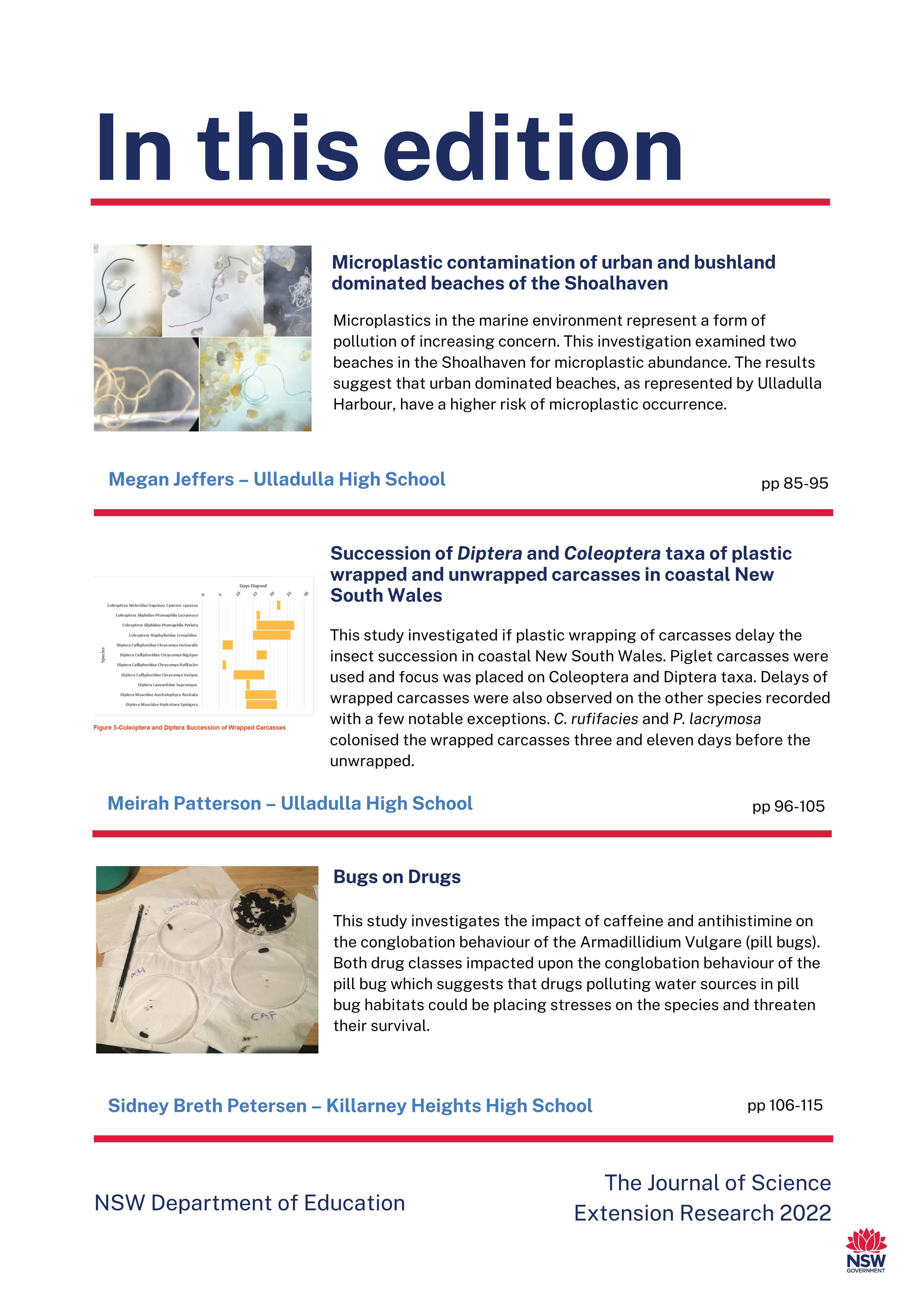
Figure 1: Stress-strain curves for LDPE irradiated with 3 different frequencies and one control group. A: No light exposure, B: Green, C: Red, D: Blue. Obtained through the analysis of recorded videos by taking a point of stress and pairing it with a point of strain. The shape of each curve is due to the relationship between the stress and strain as a material deforms. As the graph increases linearly at the beginning, stress and strain are directly proportional, however, the material later begins to stretch and deform proportionally more than the stress on it increases. This is due to the amount that the material stretches. Finally, the small inflection at the end occurs as the material reaches its breaking point and snaps, with the upwards inflection being caused by a sudden increase in the stress on the material as it is unable to stretch any further. Stress was measured to an accuracy of 4 significant figures and strain to an accuracy of 5 significant figures.
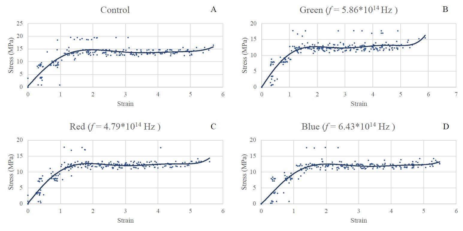
Figures 2 and 3 shown below demonstrate the statistical significance of measurements taken. For the strain data in figure 1, it has been concluded that there is no relationship between the exposure to any frequency of light and
the strain on the material (p > α). For the stress on the test strips, there was a proven link between the stress that the material was able to withstand before breaking and the frequency of the light that it was exposed to (p < α).
5.RESULTS
The Journal of Science Extension Research – Vol. 1, 2022 education.nsw.edu.au 16
6.DISCUSSION
6.1 Significance of results
LDPE was irradiated with three different frequencies of light: 4.79 ∗ 1014 Hz (red), 5.86 ∗ 1014 Hz (green) and 6.43 ∗ 1014 Hz (blue). After 128h of exposure, the LDPE was tested for its breaking stress and strain to determine if the frequency of
light that LDPE is exposed to affects its mechanical properties. Outliers were excluded at a boundary of 2 standard deviations from the mean. After outlier exclusion, a one-tailed t-test was conducted comparing the coloured sample mean to the control group mean in both the stress and strain relationships (see Figure 2 and Figure 3 descriptions for confidence intervals).
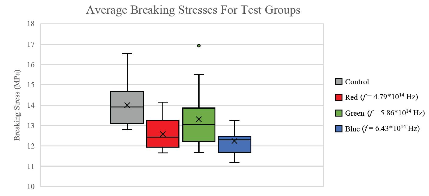
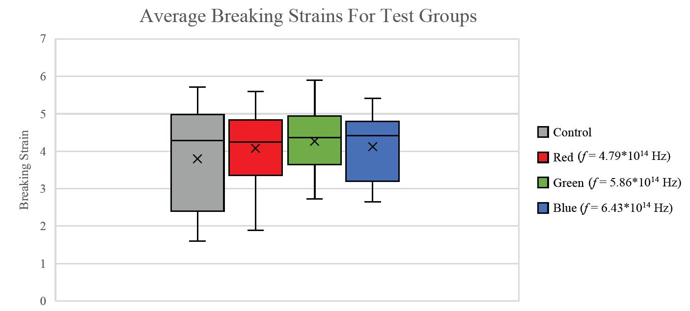 Figure 2: Average breaking strain for three different light frequencies. P-values for difference from the control mean: Red: 0.21; Green: 0.094; Blue: 0.18.
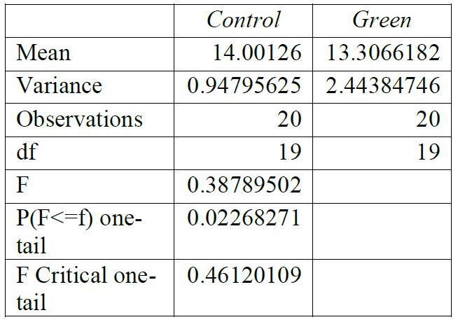
Figure 3: Average breaking stress for three different light frequencies. P-values for the difference from the control mean: Red: 2.7*10-6; Green: 0.050; Blue: 9.6*10-9.
Figure 2: Average breaking strain for three different light frequencies. P-values for difference from the control mean: Red: 0.21; Green: 0.094; Blue: 0.18.
Figure 3: Average breaking stress for three different light frequencies. P-values for the difference from the control mean: Red: 2.7*10-6; Green: 0.050; Blue: 9.6*10-9.
The Journal of Science Extension Research – Vol. 1, 2022 education.nsw.edu.au 17
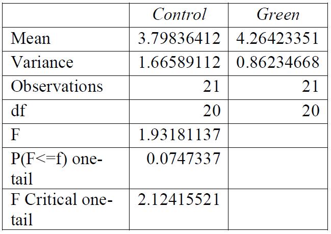
For all breaking stresses, there was a significant reduction in the tensile strength of the material leading to the on average lower breaking stresses of 12.6 MPa, 13.3 MPa and 12.2 MPa for red, green, and blue, respectively compared to the initial 14.0 MPa from the control group (p < 0.05). For the breaking strains, there was no significant reduction by any colour of light (p > 0.05).
6.2 Comparing to the literature
Based on a study of the mechanical properties of LDPE conducted by Jordan et al. (2016), the true stress, acting on LDPE upon breaking was 19 MPa. However, this data uses true stress which considers the change in the thickness of the material, whereas the data collected her measures nominal stress, which does not consider the change in the width of the material (since ������������������������ =
) and so achieves the control value of 14.0 MPa. It also uses a slightly different strain rate of 0.2 s-1 , compared to 1.17s-1, although this variation should not make a large impact. Since the strain rate used in this investigation was higher than that used by Jordan et al. 2016, the results should have shown a higher breaking stress. This can be accounted for by several factors including the aforementioned slight difference in measuring the true stress versus nominal stress. There is a potential for a difference in crystallinity to impact the results (Jordan et al. 2016) and a difference in molecular weight to impact the results (Balani et al. 2015)
Crystallinity is the degree of ordered packing in the polymer molecules (Balani et al. 2015). Tighter molecule packing creates a stronger material since intermolecular forces are stronger.
Molecular weight also has the potential to slightly impact the results, but only if the molecular weight of the polymer used in this investigation was exceptionally low or the one used by Jordan et al. (2016) was exceptionally high (Balani et al. 2015) Since both these factors can impact the strength of the polymer, this limits the ability to compare the data gathered in this experiment to other studies.
6.3 Experimental Design
During the irradiation process, the temperature was kept relatively constant at between 14.5°C and 17.5°C with an average temperature of 16°C. This temperature was kept cooler to minimise the impact of thermal degradation, although degradation generally occurs at much higher temperatures, beginning significantly at roughly 700 K depending on the rate of heating (Das & Tiwari 2017). For the same reasons, testing was conducted at 20°C to limit the effect of temperature on the results, since according to Kelly and White (1996), the temperature at which the test is conducted does matter.
Stress was measured to 4 significant figures using a digital force meter and strain was measured to 5 significant figures using Adobe Premiere Pro’s position indicator (see appendix for more detail) so there is a high degree of precision in the measurements.
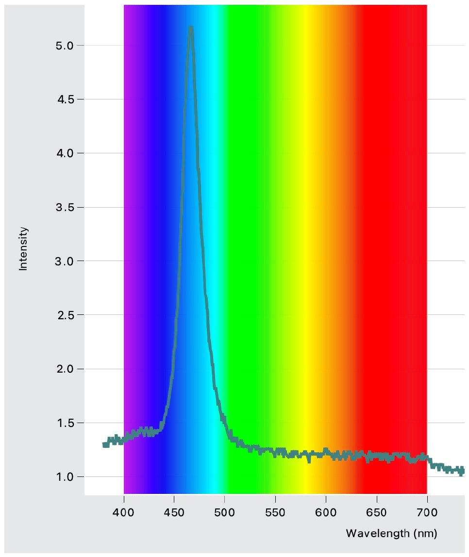
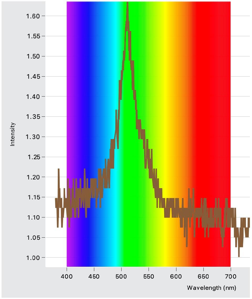
Each light colour had a small variation in its intensity (see appendix for intensity graphs). This means that exposure to each colour can only be compared independently to the control group and not between colours.
Certain tests were deemed invalid for several reasons. Primarily a test was
�������������������� �������������������� ������������������������������������ ����������������
The Journal of Science Extension Research – Vol. 1, 2022 education.nsw.edu.au 18
deemed invalid if the digital scale tipped too far to the side, making the display unreadable. Tests could also be deemed invalid if the digital scale locked itself on a specific force reading, however, this only happened once.
6.4 Sources of error
The greatest potential for random error occurs from how each test strip was cut. During preliminary investigation, it was found that slightly compromising the plastic with a cut that was perpendicular to the direction of the applied force significantly decreased the tensile strength of the material. Because of this, when the plastic was cut out of the original sheet it was ensured that the razor knife did not create any cuts in the sides of the plastic, although, it should be noted that there is still the potential for this factor to affect the results. This was compensated for by the large sample size of 25 tests for each colour, including any outliers and tests deemed invalid. The sample size remained large enough to compensate for these random errors.
There is a slight capacity for systematic error in this investigation. The clamp that held the test strips applied a slight weight force to the test strips and so may have increased the observed stress on the material. It is also not discernible if this had any bearing on the results since as discussed under section 5.2, the values cannot reasonably be compared to other studies.
6.5 Future testing
For future testing directions, the molecular weight and the degree of crystallinity should be determined so the results can be compared to other studies. Given that Jordan et al. (2016) uses true
stress, the true stress of the material should be calculated alongside the nominal stress of the material.
Since red light was shown to have a significant impact on the breaking stress of LDPE, future experimentation should extend this to lower frequencies including infrared light. Conversely, to investigate if photodegradation will, at any point, impact the breaking strain of LDPE. In future investigations, a lighter clamp should also be used as the weight of the clamp could increase the reading on the scale which would increase the observed stress on the material.
Future testing should also investigate the effect of visible light intensity of a specific frequency on the breaking stress and strain of LDPE as each light colour had a different intensity.
7.CONCLUSION
The relationship between the frequency of light that LDPE is exposed to compared to the breaking stress and strain was investigated. It was found that all three frequencies of light (red: 4.79 ∗ 1014 Hz; green: 5.86 ∗ 1014 Hz; blue: 6.43 ∗ 1014 Hz) made a significant impact on the breaking stress of LDPE, however, there was no relationship between the breaking strain and the exposure to visible light for short time frames of 128 hours. Thus, the hypothesised result for this experiment that as the frequency of light increases, there will be a reduction in breaking stress and strain, is only partially correct.
The result serves as a measurement device to quantitatively track the photodegradation of LDPE under visible light.
The Journal of Science Extension Research – Vol. 1, 2022 education.nsw.edu.au 19
This result is not reflective of a similar test conducted by Liu et al. (2013), which used the lack of mass reduction in the polymer to show that there was no degradation under short term visible light exposure. Similarly, Venkataramana et al. (2020) showed that photodegradation by visible light would occur when catalysed. Despite this divergence from the existing literature, tests were conducted validly, therefore, it is reasonable to conclude that breaking stress is affected by exposure to visible light frequencies while breaking strain is not.
8.REFERENCES
1. Balani, K, Verma, V, Agarwal, A & Narayan, R 2015, Physical, thermal and mechanical properties of polymers, John Wiley & Sons, Inc, viewed 5 August 2021, https://onlinelibrary.wiley.com/doi/10.1002 /9781118950623.app1
2.Das, P & Tiwari, P 2017, ‘Thermal degradation kinetics of plastics and model selection’, Thermochimica Acta, vol. 654, pp. 191-202
3.Feng,L & Jasiuk, I 2010, ‘Effect of specimen geometry on tensile strength of cortical bone’, Journal of Biomedical Materials Research Part A, vol. 95A, no. 2, pp. 580-587
4.Gewert, B, Plassmann, M, Sandblom, O & MacLeod, M 2018, ‘Identification of chain scission products released to water by plastic exposed to ultraviolet light’, Environmental Science and Technology Letters, vol. 5, pp. 272-276
5.Jordan, J.L, Casem, D.T, Bradley, J.M, Dwivedi, A.K, Brown, E.N & Jordan, C.W 2016, ‘Mechanical properties of lowdensity polyethylene’, Journal of Dynamic Behaviour of Materials, vol.2, 411-420
6.Kelly, C.T & White, J.R 1996 ‘ Photodegradation of polyethylene and polypropylene at slow-strain rate’, Polymer Degradation and Stability, vol. 56, pp. 367-383
7.Khanam, P.N, AlMaadeed, M.A.A 2015, ‘Processing and characterization of polyethylene-based composites’, Advanced Manufacturing: Polymer & Composites Science, vol. 1, no. 2, pp. 6379
8.Liu, G, Liao, S, Zhu, D, Hua, Y & Zhou, W 2012, ‘Innovative photocatalytic degradation of polyethylene film with boron-doped cryptomelane under UV light irradiation’, Chemical Engineering Journal, vol. 213, pp. 286-294
9.Ojeda, T 2013, Polymers and the environment, InTech, viewed 2 February 2021, <https://www.intechopen.com/chapters/4 2104>
10. Plastics – the facts 2018 2018, PlasticsEurope, Brussels, Belgium
11.Schnabel, W 2014, Polymers and Electromagnetic Radiation, Wiley-VCH Verlag GmbH & Co. KGaA, Boschstr, Weinheim, Germany
12. Stress-strain relationships 2013, University of Arizona, viewed on 1 March 2021, http://www.docdatabase.net/morestress-strainrelationships-the-universityof-arizona--1114894.html
13.Rabek, J.F 1995, Polymer photodegradation: Mechanism and experimental methods, Chapman and Hall, London, Uk, viewed 5 July 2021, https://books.google.com.au/books?hl=en &lr=&id=dXwbS128lXoC&oi=fnd&pg=PR1 5&dq=rabek+1994&ots=V_9OokzrbV&sig
The Journal of Science Extension Research – Vol. 1, 2022 education.nsw.edu.au 20
=nmtNYkZVetk8o12OAJLIS1qTj5mU&red ir_esc=y#v=onepage&q=rabek%201994& f=false
14.Reusch, W 2015, Free radical polymerization,Chemistry LibreTexts, viewed 18 June 2021, https://chem.libretexts.org/Courses/Purdu e/Purdue_Chem_26100%3A_Organic_C hemistry_I_(Wenthold)/Chapter_08%3A_ Reactions_of_Alkenes/8.7.%09Polymeriz ation/Free_Radical_Polymerization
9.APPENDIX
15.Venkataramana, C, Botsa, S.M, Shyamala, P & Muralikrishna, R 2020, ‘Photocatalytic degradation of polyethylene plastics by NiAl2O4 spinelssynthesis and characterization’, Chemosphere, https://doi.org/10.1016/j.chemosphere.20 20.129021
16.Yousif, E, Haddad, R 2013, ‘Photodegradation and photostabalization of polymers, especially polystyrene: review’, SpringerPlus, vol. 2, no. 398
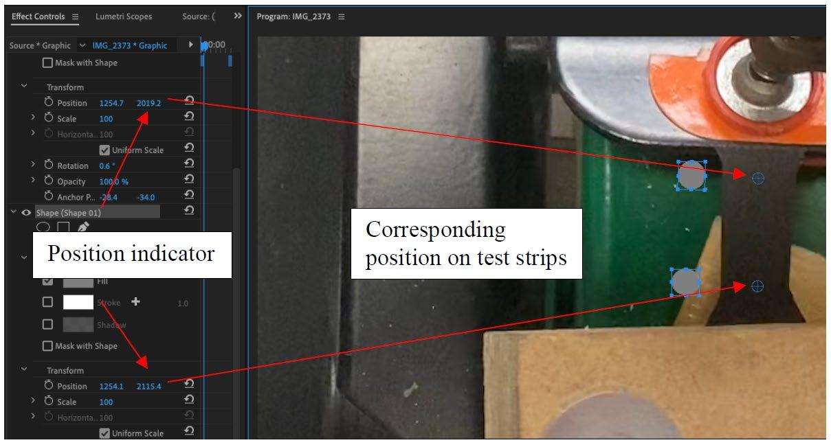
Image 2: Demonstration of how the Adobe Premiere Pro position indicator is used to determine strain to 5 significant figures. The position indicator changes with the position of the corresponding crosshair. The crosshair is positioned on the inside edge of the marking during analysis and the displacement between the two crosshairs is measured through the use of the position indicator. This is then compared to the initial length of the test strip, measured by the same method.
The Journal of Science Extension Research – Vol. 1, 2022 education.nsw.edu.au 21
Table 1: F-test for control group compared to red light exposure. Conclusions: variance was unequal.
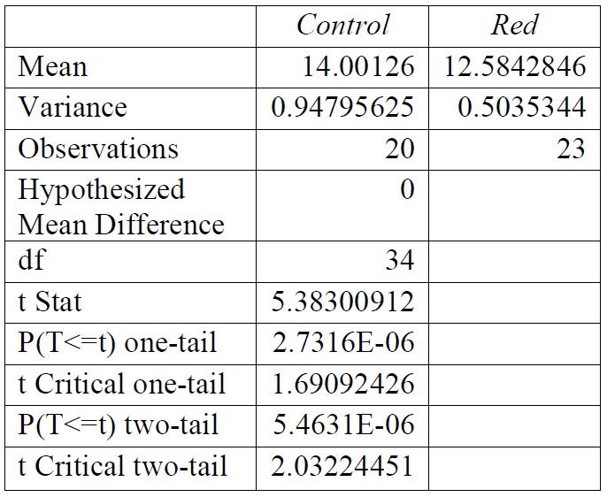
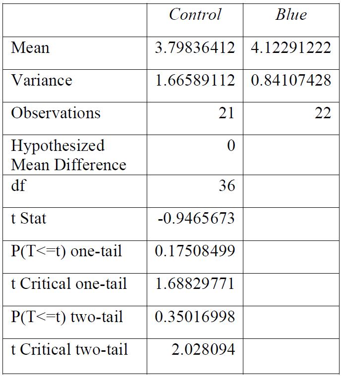
Table 3: F-test for control group compared to blue light exposure. Conclusions: variance was equal.
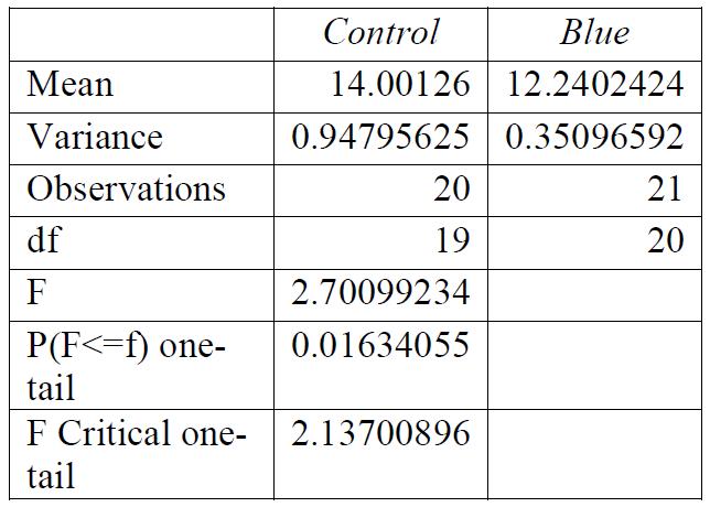
Table 2: F-test for control group compared to green light exposure. Conclusions: variance was equal.
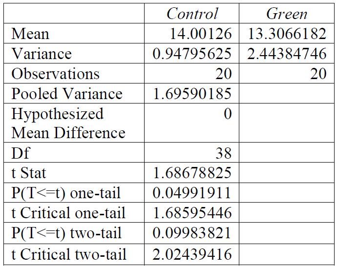
Table 4: T-test for control group compared to red light exposure. Conclusions: there was a significant relationship between the light exposure and the breaking stress.
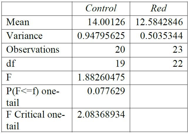
Table 5: T-test for control group compared to green light exposure. Conclusions: there was a significant relationship between the light exposure and the breaking stress.
(Tables 1 – 6)
Stress Statistical Analysis Tables
The Journal of Science Extension Research – Vol. 1, 2022 education.nsw.edu.au 22
Strain Statistical Analysis Tables (Tables 7 – 12)
Table 6: T-test for control group compared to blue light exposure. Conclusions: there was a significant relationship between the light exposure and the breaking stress.
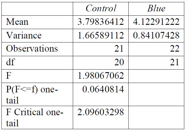
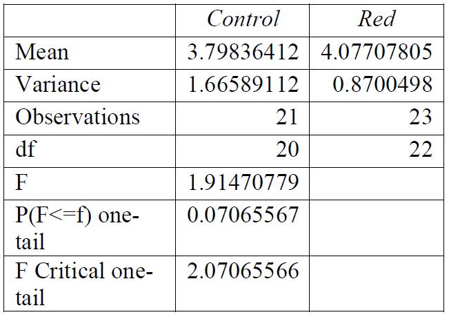
Table 7: F-test for control group compared to red light exposure. Conclusions: variance was unequal.

Table 9: F-test for control group compared to blue light exposure. Conclusions: variance was unequal.
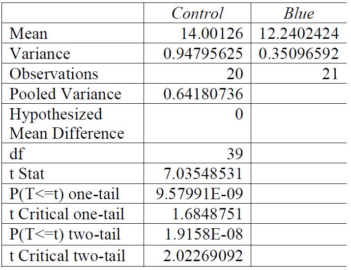
Table 8: F-test for control group compared to green light exposure. Conclusions: variance was unequal.
Table 10: T-test for control group compared to red light exposure. Conclusions: light exposure made no significant impact to the breaking stress.
The Journal of Science Extension Research – Vol. 1, 2022 education.nsw.edu.au 23
Conclusions: light exposure made no significant impact to the breaking stress.
Light Intensity Graphs (Figures 4 – 6)
Conclusions: light exposure made no significant impact to the breaking stress.
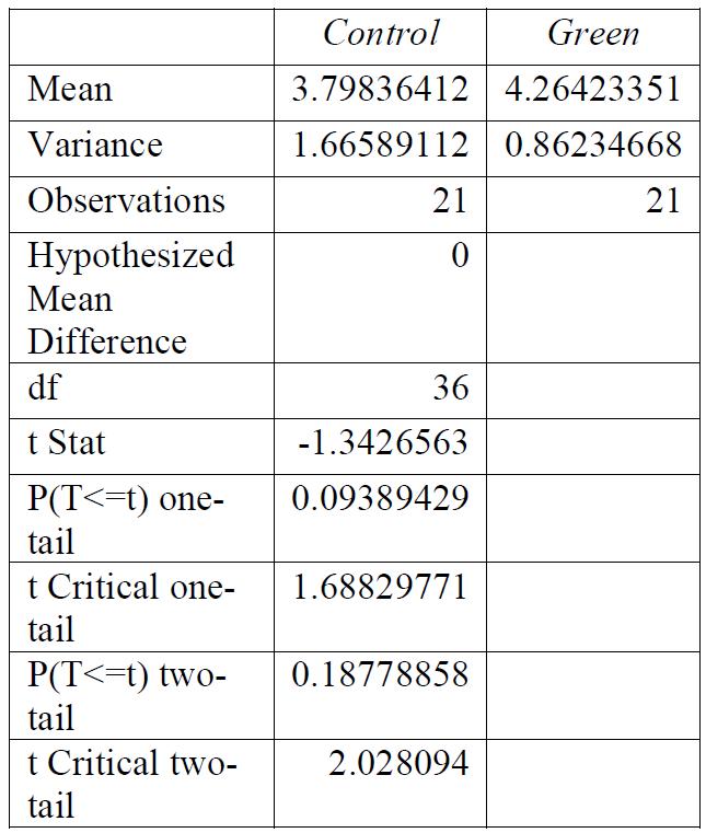 Table 11: T-test for control group compared to green light exposure.
Table 12: T-test for control group compared to blue light exposure.
Figure 4: Intensity and wavelength graph for the green LED lights used
Table 11: T-test for control group compared to green light exposure.
Table 12: T-test for control group compared to blue light exposure.
Figure 4: Intensity and wavelength graph for the green LED lights used
The Journal of Science Extension Research – Vol. 1, 2022 education.nsw.edu.au 24
Figure 5: Intensity and wavelength graph for the blue LED lights used.
Processed Breaking Stress Data
Processed Breaking Strain Data
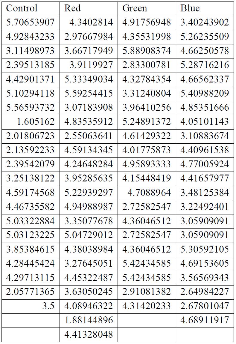
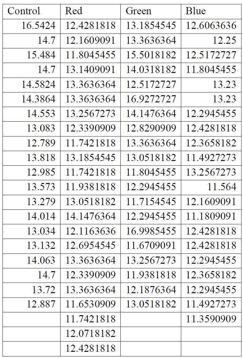
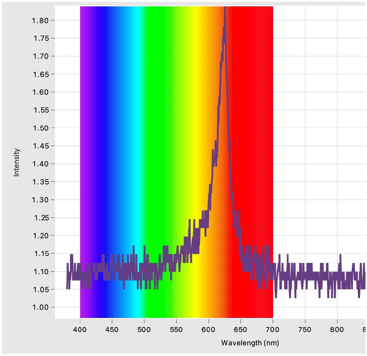 Figure 6: Intensity and wavelength graph for the red LED lights used.
Table 13: Processed breaking stress data following outlier exclusion. All values in MPa.
Figure 6: Intensity and wavelength graph for the red LED lights used.
Table 13: Processed breaking stress data following outlier exclusion. All values in MPa.
The Journal of Science Extension Research – Vol. 1, 2022 education.nsw.edu.au 25
Table 14: Processed breaking strain data following outlier exclusion.
Voltage and its effect on the rate of Sodium Hydroxide production in Membrane Cells
Isla Jones St Ives High School
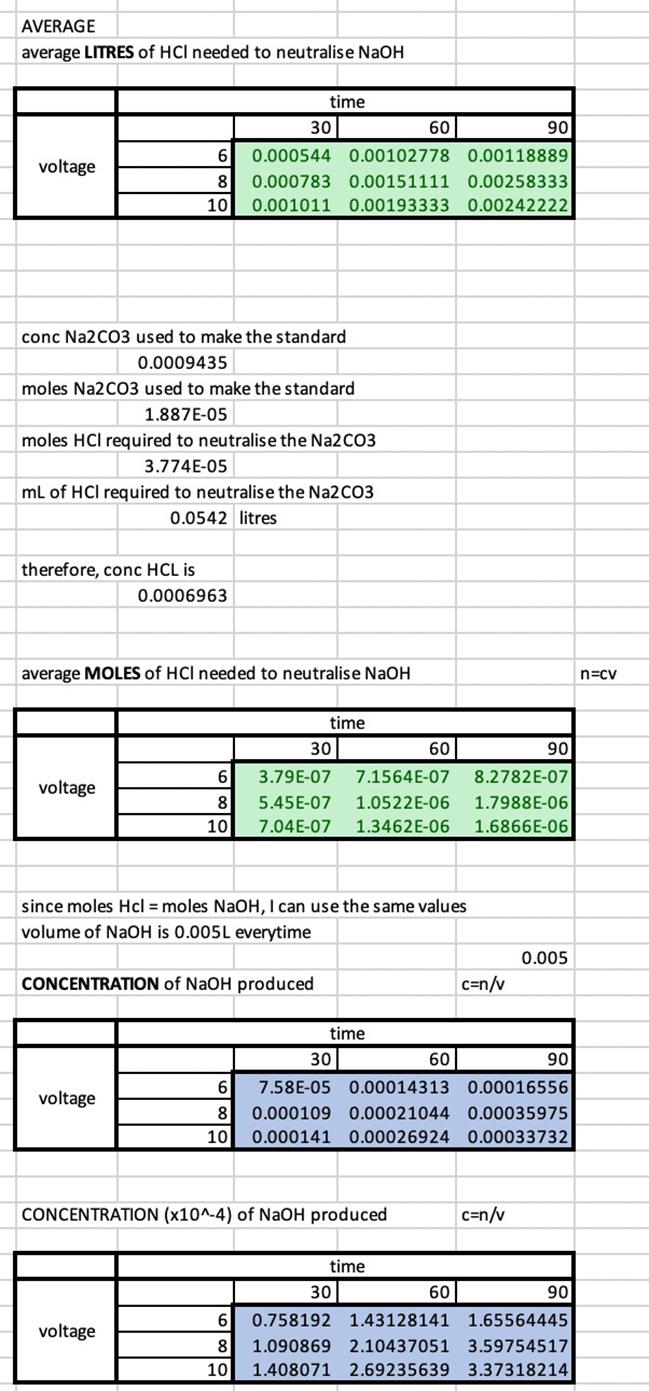
Membrane cells containing electrolytes powered by a potential difference are the primary technology used to produce sodium hydroxide. The optimal conditions of membrane cells have been the subject of multiple investigations. This report outlines an investigation into the effect of voltage on the rate of sodium hydroxide production in membrane cells. Sodium hydroxide was produced by a means of electrolysis in a membrane cell from a saturated solution of sodium chloride. Experiments were carried out at voltages of 6V, 8V and 10V for various periods of time. The sodium hydroxide solutions produced were titrated against a standard solution of hydrochloric acid and their concentrations were calculated. Limitations in this experiment meant that the data collected was unable to show a statistically significant difference in the rate of sodium hydroxide production at different voltages for a confidence interval of 95%. However, there is a positive correlation between increased voltage and rate of reaction to a confidence interval of 80%
LITERATURE REVIEW
Sodium hydroxide (NaOH) is a highly basic, inorganic compound used in the manufacture of products such as detergents, pharmaceuticals, paper and the food industry (Chlor-alkali industry review 2019-2020, 2020). Sodium hydroxide is produced in conjunction with chlorine and hydrogen gas as a part of the chlor-alkali industry. This industry accounts for 55% of all chemical manufacture in EU-27 and EFTA countries (Brinkmann et al., 2014). As such, the electrochemical processes used in manufacture are designed to maximise the rate of production at the lowest possible cost to corporations (Brinkmann et al., 2014).
There are three primary types of electrolytic cell used in the chlor-alkali industry; mercury cells, diaphragm cells
and membrane cells (Cardarelli, 2008). Of these technologies, both mercury and diaphragm cells pose serious environmental concerns due to their reliance on mercury and asbestos respectively (Crook and Mousavi, 2016). Concerns regarding mercury waste include the accumulation of mercury in aquatic ecosystems and the human health risks associated with consuming affected seafood (Sanborn and Brodberg, 2006). Similarly, the use of asbestos in diaphragm cells induces irreversible health conditions in workers (Crook and Mousavi, 2016). Due to these environmental concerns and recent environmental protection laws, membrane cells are the preferred technology accounting for 83% of the chlor-alkali industry’s production in Europe (Chloralkali industry review 2019-2020, 2020).
The industrial shift towards membrane technology is the reason why this
The Journal of Science Extension Research – Vol. 1, 2022 education.nsw.edu.au 26
investigation was specifically conducted on membrane cells. However, it is understood that this investigation is merely a model of an industrial process to investigate relationships and that any results are not necessarily applicable on an industry scale.
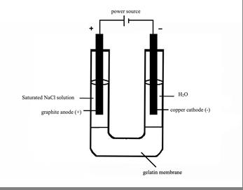
Membrane cells consist of two inert electrodes separated by a semipermeable membrane which acts as an ion exchanger (Domga et al., 2017). In membrane cells, a potential difference is applied over the electrodes to initiate the electrochemical reaction (Cardarelli, 2008). Due to this potential difference and flow of electrons, the anode and cathode are oppositely charged and attract chlorine and sodium ions respectively. It is the negatively charged cathode that provides attractive force to the positively charged sodium ions, enabling them to pass through the membrane (Domga et al., 2017). The membrane is usually made from polytetrafluoroethylene (PTFE) (Crook and Mousavi, 2016). However, due to limitations in equipment, this investigation was conducted using gelatin as a substitute for the semipermeable membrane. Gelatin was chosen as it creates a seal with the sides of the test tube, restricting the flow of solutions and only allowing ions to migrate between compartments. However, in pilot studies it was observed that the membrane began to break or separate from the test tube at around 120 minutes. As such, gelatin is by no means a perfect substitute for an ion exchange membrane due to its lack of longevity.
This study aims to investigate the effect of different voltages on the rate of sodium hydroxide in membrane cells. To inform initial experimental design and the alternate hypothesis, other investigations
in this field of study have been subject to review.
The minimum cell voltage for electrolysis is calculated using reduction potentials and experimentally determined to be 2.83V by Domga et al. in their 2017 study on electrolysis parameters in membrane cells. Their results indicate that when the distance between electrodes is increased, the cell voltage also increases proportionally to maintain a constant conductivity of the solution (Domga et al., 2017)(Rosales- Huamani et al., 2021.). As such, it was hypothesised that if voltage was increased and distance was controlled, the conductivity of the cell would increase. An increase in electrical conductivity of a cell is directly proportional to the flow of electrons through the circuit. As such, if an increase in voltage increases the flow of electrons, the rate of reaction will be increased for the production of NaOH.
SCIENTIFIC RESEARCH QUESTION
How does voltage affect the rate of sodium hydroxide production in membrane cells?
SCIENTIFIC HYPOTHESIS
An increase in the input voltage of a membrane cell will increase the rate of sodium hydroxide production.
METHODOLOGY
Preparation of Solutions and Membranes
A 12.5% w/v solution of gelatin was prepared by dissolving gelatin powder in room temperature water. The solution was brought to boiling point and 15mL of liquid was pipetted into each u-tube. The
The Journal of Science Extension Research – Vol. 1, 2022 education.nsw.edu.au 27
membranes were placed into a fridge left to set for a minimum of 12 hours.
To prepare the sodium chloride solution, NaCl was dissolved in distilled water until the solution was saturated. Blue food dye was also added to this solution to visually monitor defects in the membrane.
Preparation of Electrodes and Assembly
The electrodes used for this experiment were a graphite anode and a copper cathode. Before each trial, both electrodes were rinsed with distilled water and sanded down with steel wool. They were then weighed, attached to alligator clips and suspended at a controlled height above the membrane.
(left) side of the membrane and 20mL of distilled water (H2O) was added to the cathode (right) side of the membrane.
Production of Sodium Hydroxide
The membrane cell’s DC power supply was turned on and run at one of three different voltages (6V, 8V or 10V) for a given time period (30, 60 & 90 mins). Once the power was turned on, the initial current running through the set-up was recorded. At the end of the time period, the change in current was noted down and the power was turned off. Both electrodes were removed from the solution, dried and weighed. The NaOH sample was extracted from the cell and transferred into conical flasks for titrations.
Titrations
Immediately after collecting a NaOH sample, a drop of phenolphthalein was added to 5mL of the sample and titrated against a standard solution of hydrochloric acid (HCl). The volume of HCl required to neutralise the NaOH was recorded and the process was repeated twice for the sample. The volume of HCl required to neutralise the samples was then used to calculate the concentration of each sample.
Figure 1 – the experimental set up
As seen in Figure 1 (above), 20mL of NaCl solution was added to the anode
The Journal of Science Extension Research – Vol. 1, 2022 education.nsw.edu.au 28
RESULTS
Analysis was performed using a combination of linear regression and t-tests.
Each point is an average of three NaOH samples, all of which have been titrated three times. The R² values for each voltages’ trend is high (between 0.9 and 1), indicating a strong, positive correlation between time and the concentration of NaOH at the respective voltage. The difference in the coefficient of x between the equations of the trendlines indicates that there is a difference in the gradient, as visually depicted in the graph. This difference in gradient shows that there is a difference of the rate of sodium hydroxide production. To investigate the significance of this difference, a series of t-tests were required.
Whilst the none of differences between voltages at each time have been shown to be significant for a p-value of 0.05, there are some significant differences for a p-value of 0.20. The difference between 6V and 10V has been shown to be
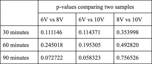
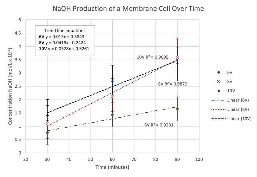 Figure 2 A concentration vs time graph depicting the rate of NaOH production at different voltages.
Figure 3: Table of p-values depicting the significance of a difference in the NaOH concentration.
Figure 2 A concentration vs time graph depicting the rate of NaOH production at different voltages.
Figure 3: Table of p-values depicting the significance of a difference in the NaOH concentration.
The Journal of Science Extension Research – Vol. 1, 2022 education.nsw.edu.au 29
significant at all times with an 80% confidence interval. Similarly, the difference between 6V and 8V at times of 30 and 90 minutes are shown to be statistically significant for a p-value of 0.20, indicating a confidence interval of 80%. However, at a p value of 0.20, there is still no statistically significant difference in the rate of NaOH production between 6V and 8V at a time of 60 minutes and between 8V and 10V at all times.
The difference in initial and final weight of both electrodes was negligible for every trial. On the other hand, the change in current during each trial was unpredictable and there appears to be no real relationship.
DISCUSSION
The results of this experiment yielded several trends worthy of discussion. Both the R² values and the respective gradients of each voltage series provide insights into the relationships between voltage and NaOH production.
From the high R² values and positive correlation for each voltage trend, it can be determined that an increase in time results in an increased concentration of NaOH at all voltages.
A similar trend has been observed in comparable experiments, including an experiment on the factors influencing sodium hydroxide production conducted by Rosales-Huamani et al., 2021. As longer exposure to the power supply continued to increase the concentration of NaOH, further experimentation and analysis of the cell efficiency would be required to determine the optimum time frame of operation.
The difference in gradients of voltage series and thus the rate of reaction is not considered statistically significant at a 95% confidence interval, however, some differences are statistically significant at a confidence interval of 80%. The greatest difference in rate of reaction is between the 6V series and the 10V series. This supports results found by Domga et al., 2017 and Rosales-Huamani et al, 2021; a greater potential difference between the electrodes results in a solution with increased conductivity. This increased conductivity is indicated by the increased rate of production of NaOH.
Sources of Error
The greatest potential for random error in this experiment was the positioning of the electrodes above the membrane. As confirmed in a study on the relationship between resistance and conductivity of electrodes, an increased distance between electrodes reduces their conductivity (Cosoli et al., 2020). Despite efforts to control the distance between electrodes, there is potential for this factor to affect the results.
There was a complication with one of the alligator clips several trials into data collection. This clip was replaced within a new wire of the same length, however, there is a potential random error as result of a difference in conductivity of the two wires. Due to time constraints the trials conducted with the first wire were unable to be revised.
Another potential source of error for this experiment was the low concentrations and small volumes of the NaOH solutions. Due to limitations of equipment, the concentration of NaOH produced was relatively low. To titrate each sample multiple times, only small volumes of
The Journal of Science Extension Research – Vol. 1, 2022 education.nsw.edu.au 30
solution were available. These small volumes led to high relative uncertainty for each titration and consequently reduced the reliability of the investigation.
Limitations and Further Research
This investigation and the conclusions that can be drawn from its data are fairly limited. The combined nature of the small data set and high variance between trials means that it was difficult to identify and remove outliers. In further research, the size of this study could be expanded to provide more data and reduce the margin of error, increasing reliability.
Another limitation of this investigation was the nature of the gelatin membrane. Whilst it held up well for the time frames proposed in this study, in initial tests defects were observed in the membrane from times onwards of 120 minutes. This indicates that the reliability of a gelatin membrane decreases over time and as such, to expand the scope of the investigation to longer time frames, the use of a different type of membrane would be necessary.
CONCLUSION
This report investigated the effects of voltage on the rate of sodium hydroxide production in membrane cells. It was found that an increase in time resulted in an increased concentration of sodium hydroxide at all voltages. However, the results indicate that there was not a statistically significant difference between the rate of sodium hydroxide production at these voltages for a confidence interval of 95%. While this does not provide a conclusive relationship between voltage and rate of sodium hydroxide production, the data does suggest a relationship between the variables at a confidence
interval of 80%. The reduced confidence in the relationship is due to the potential for error in this investigation. Further study will include obtaining a larger data set to increase the reliability of the data, thus reducing the margin of error.
REFERENCES
2020. Chlor-alkali industry review 20192020. [ebook] EuroChlor. Available at: <https://www.chlorineindustryreview.com/ wp- content/uploads/2020/09/IndustryReview-2019_2020.pdf> [Accessed 16 September 2021].
Brinkmann, T., Santonja, G., Schorcht, F., Roudier, S. and Delgado Sancho, L., 2014. Best Available Techniques (BAT) Reference Document for the Production of Chlor-alkali
Cardarelli, F., 2008. Materials Handbook. A Concise Desktop Reference 2nd ed. Springer.
Cosoli, G., Mobili, A., Tittarelli, F., Revel, G. and Chiariotti, P., 2020. Electrical Resistivity and Electrical Impedance Measurement in Mortar and Concrete Elements: A Systematic Review. Applied Sciences, 10(24), p.9152.
Crook, J. and Mousavi, A., 2016. The chlor- alkali process: A review of history and pollution. Environmental Forensics, 17(3), pp.211-217.
Domga, R., Noumi, G. and Tchatchueng, J., 2017. Study of Some Electrolysis Parameters for Chlorine and Hydrogen Production Using a New Membrane Electrolyzer. International Journal of Chemical Engineering and Analytical Science, 2(1), pp.1-8.
The Journal of Science Extension Research – Vol. 1, 2022 education.nsw.edu.au 31
Rosales-Huamani, J., Medina-Collana, J., Diaz-Cordova, Z. and Montaño-Pisfil, J., 2021. Factors Influencing the Formation of Sodium Hydroxide by an Ion Exchange Membrane Cell. Batteries, 7(2), p.34.
Sanborn, J. and Brodberg, R., 2006. EVALUATION OF BIOACCUMULATION FACTORS AND TRANSLATORS FOR METHYLMERCURY. California: State of California.
APPENDIX
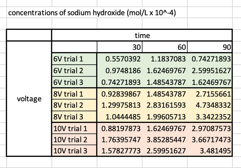
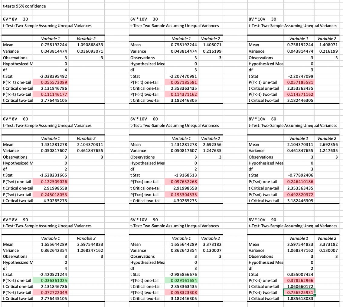 Figure 4: Concentrations of sodium hydroxide for each trial
The Journal of Science Extension Research – Vol. 1, 2022 education.nsw.edu.au 32
Figure 5: T-test calculations for 95% confidence

The Journal of Science Extension Research – Vol. 1, 2022 education.nsw.edu.au 33
Figure 6: T-test calculations for 80% confidence.
The Journal of Science Extension Research – Vol. 1, 2022 education.nsw.edu.au 34
Figure 7: Additional calculations
The clash of the modern crises: A study investigating the development of antibiotic resistance in Escherichia coli under increasing carbon dioxide concentrations
Tahlia Martignago Menai High School
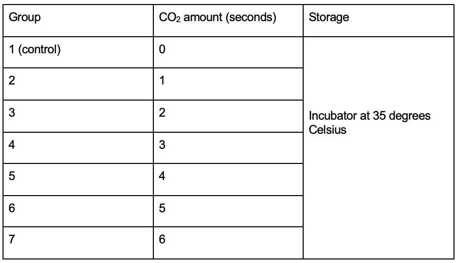
The global crisis of increasing atmospheric carbon dioxide concentrations has resulted in changes in biological processes and systems, whereby carbon dioxide has been shown to affect mutation in organisms such as bacteria and fungi. In the context of the increasing prevalence of antibiotic resistance, it is unclear whether carbon dioxide may impact the development of antibiotic resistance in bacteria. This primary study aimed to investigate if differing concentrations of carbon dioxide affected the rate and extent of antibiotic resistance developed by Escherichia coli over 4 generations using the Kirby Bauer disk diffusion method and MIC test strips. It was found that increased carbon dioxide exposure resulted in significant increases in both the extent and rate of antibiotic resistance acquired by E.coli, where P=0.04 and P=0.008 respectively. Further investigation through refining and replicating the method is required to support the link between increases in global atmospheric carbon dioxide concentrations and increases in antibiotic resistance of bacteria, which may pose a major public health issue in terms of the treatment of infectious disease.
LITERATURE REVIEW
Carbon dioxide is a large factor in the climate emergency due to its contribution to the greenhouse effect, responsible for approximately ¾ of emissions of GHG. In November 2020, global atmospheric CO2 concentrations were at 415ppm, approximately 47% greater than preindustrial levels in 1850 (NASA, 2021). Increases in CO2 concentrations have been shown to increase mutation frequency (H. P. Charles & Gillian A. Roberts, 1967; Ezraty, B et al., 2011), cell membrane permeability (Endeward, V. et al., 2017) and promote the dissemination of antibiotic resistance genes in bacteria (Liao, J., Chen, Y., & Huang, H., 2019). Worst-case projections predict an
increase from current concentrations by 1000 - 2100ppm (Nakicenovic et al, 2000), which would result in greater impacts than already seen in biological systems. Antibiotic resistance is one of the largest growing public health issues globally and is a result of bacterial mutation. The increase in both atmospheric CO2 concentrations and prevalence of antibiotic resistance alongside the known mutagenic effect of CO2 on biological systems, has attracted the investigation of the effects of carbon dioxide on the development of antibiotic resistance.
Carbon dioxide has been shown to act as a growth factor for some mutations of the fungi Neurospora (Reissig & Nazario, 1962; Charles & Broadbent, 1964). A
The Journal of Science Extension Research – Vol. 1, 2022 education.nsw.edu.au 35
study conducted by Charles & Roberts (1968) investigated whether the effects observed are limited to Neurospora, testing on E.coli. The study found that mutations of E.coli were largely seen in gas phases containing 20% CO2. It also found that the same mutations occur in E.coli as in Neurospora, which could suggest an impact on a wider variety of microorganisms due to increased CO2 involvement. However, the way in which CO2 stimulates mutations was not established, and the investigation failed to mention the rate or quantity of overall mutations over the range of CO2 concentrations tested, thus reducing the validity of the investigation.
These findings were supported in an investigation of mutation frequencies of E.coli in the presence of CO2 and hydrogen peroxide (Ezraty, B. et al., 2011). Higher concentrations of CO2 increased mutation rates significantly, and was shown to be linked to increased reactive oxygen species (ROS). This study suggests a link between CO2 increases and bacterial mutation, and a mechanism for how CO2 increases can result in increased mutation, however it investigated a multitude of independent variables that convoluted the aim of this investigation.
Supporting findings by Ezraty, B. et al. (2011), a 2019 study also showed that samples treated with CO2 produced more reactive oxygen species (ROS) compared to controls, indicating that CO2 promoted ROS production in E.coli (Liao, J., Chen, Y., & Huang, H. 2019). The increase of ROS production, induced by CO2 exposure, resulted in DNA and cell membrane damage, which affected the structure of the cells and increased cell membrane permeability, and promoted
the transformation of antibiotic resistant genes (ARG) by 1.5 - 5.5 and 1.4 - 4.5 fold in two strains of E.coli respectively after being treated with CO2 (Liao, J., Chen, Y., & Huang, H. 2019). Since ROS can be attributed to DNA damage and mutation, this study provided a mechanism for the development and transfer of ARGs between bacteria, thus suggesting that exposure to CO2 would increase how many bacteria obtain these genes through horizontal gene transfer. Although this study consistently referred to antibiotic resistant genes, and acknowledged that further study was required to explore the effect of increased ARG transformation, it failed to show the resulting change in the extent of antibiotic resistance.
Considering the increases in mutation frequency shown in these studies, it can be inferred that carbon dioxide exposure could result in increased antibiotic resistance, however research generally focuses on the factors that could lead to antibiotic resistance particularly the effect of carbon dioxide on mutation, as well as cell damage and membrane permeability rather than the specific degree of developed antibiotic resistance. Thus, this primary investigation aims to investigate how increasing carbon dioxide concentrations affect the extent of antibiotic resistance in Escherichia coli over 4 generations to quantify the impact of mutation and other processes that occur in organisms as a result of increases in CO2 exposure outlined in these studies.
RESEARCH QUESTION
Will increased concentrations of carbon dioxide affect the extent of antibiotic
The Journal of Science Extension Research – Vol. 1, 2022 education.nsw.edu.au 36
resistance acquired by Escherichia coli over 4 generations?
SCIENTIFIC HYPOTHESIS
The cultures of E.coli exposed to increased carbon dioxide concentration are expected to develop more resistance to the antibiotic in comparison to E.coli cultures incubated in lower carbon dioxide concentrations, in accordance with studies that found increased carbon dioxide resulted in higher transformation efficiencies of antibiotic resistant genes (Liao, J., Chen, Y., & Huang, H., 2019).
VARIABLES
Independent variable: Concentration of carbon dioxide (see appendix B and E).
Dependent variable: Extent of antibiotic resistance acquired over 4 bacterial generations (diameters of zones of inhibition and MIC values).
Controlled variables:
• Type + strain of bacteria (Escherichia coli, K-12 strain)
• Antibiotic (tetracycline)
• Agar plates (Mueller Hinton, 100mm)
• Incubation temperature (35 degrees Celsius)
• Time in between inoculation and measurement (24 hours)
• Amount of initial bacteria (100 μL)
• Generations of bacteria (4 generations)
Control: Mueller Hinton agar plate inoculated with bacteria and tetracycline susceptibility disc, incubated at 35 degrees Celsius with no additional exposure to carbon dioxide.
METHODOLOGY
All methods were undertaken in a lab environment, following aseptic techniques throughout (see appendix A). Equipment setup is pictured in appendix C.
Generation 1
28 Mueller Hinton agar plates were each inoculated with 100 μL of Escherichia coli and spread to create a bacterial lawn. A tetracycline antibiotic susceptibility disc was placed in the centre of each plate (see appendix D). The 28 plates were split into 7 groups of 4 cultures. All agar plates of each group were placed in a container (7 containers in total). Carbon dioxide was pumped into each container for the required time interval detailed below before closing valves to seal the environment (see appendix B). All containers were stored in the same incubator set to 35 degrees Celsius. After 24 hours, the diameters of the zones of inhibition were recorded with a ruler and tabulated.
Generation 2 & 3
Swabs were taken of the edges of the zones of inhibition from each of the generation 1 control cultures and inoculated onto a control Mueller Hinton agar plate (see appendix F). This was
Table A – CO2 setup for bacterial groups
The Journal of Science Extension Research – Vol. 1, 2022 education.nsw.edu.au 37
repeated for each plate within each experimental group (see appendix C).
Tetracycline antibiotic susceptibility discs were placed into the centre of all plates. Each group was placed into the same carbon dioxide environments as in generation 1 and incubated at 35 degrees Celsius for 24 hours. The diameters of the zones of inhibition were recorded with a ruler and tabulated. This was repeated to create generation 3.
Generation 4
RISK ASSESSMENT
Risk Precautions
Contamination of surfaces with pathogenic bacteria
Burns to user due to open flame of bunsen burner
Growth of hazardous anaerobic bacteria
Combustion of carbon dioxide canister
RESULTS
Swabs were taken of the edges of the zones of inhibition for the generation 3 cultures and inoculated onto a corresponding agar plate as performed in generation 2 & 3. This was repeated for each experimental group. Tetracycline MIC e-test strips were placed into the centre of all plates (see appendix G). Each group was placed into the corresponding carbon dioxide environments as done in generation 1 and incubated at 35 degrees Celsius for 24 hours. The MIC values of each culture were recorded and tabulated.
All surfaces and equipment were santised before and after use and hands were washed before and after undertaking the experiment.
The flame was not left unattended. When not directly in use it was ensured that the flame was set to the “safety” setting.
Cultures were not completely sealed before or during incubation. Small amounts of tape were used to secure the lid however gaps were left to encourage airflow.
The canister was kept out of sunlight and in a well ventilated cupboard.
Zones of inhibition of all cultures were measured for generations 1-3 with a centimetre ruler 24 hours after inoculation, and generation 4 was measured through recording the MIC of each culture 24 hours after inoculation (see appendix G).
T-tests were conducted in order to compare the 2 averages of the control and the experimental groups to determine the presence of a statistically significant link between CO2 and antibiotic resistance, however the test was limited by the lack of data provided. The alpha
value chosen was 0.05, thus results that are statistically significant have at least a 95% confidence interval (see appendix H). Two-tailed P-values were used to determine if the experimental mean was significantly less or greater than the control mean.
Table B – Risk assessment
The Journal of Science Extension Research – Vol. 1, 2022 education.nsw.edu.au 38
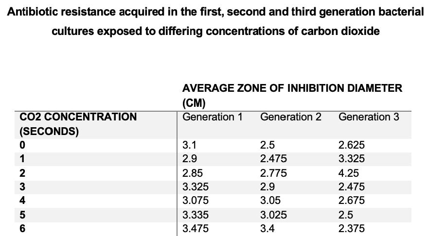
It was found that zones of inhibition of all groups generally decreased as generations progressed, whereby generation 1 had the largest zones of inhibition. The first and second bacterial generations possessed larger zones of inhibition as CO2 concentration increased. The third generation had the largest zones of inhibition at lower CO2 concentrations of 1 and 2 seconds in comparison to third generation controls. After 3 seconds, the zones of inhibition then stabilised and decreased as CO2 concentration increased in groups 4, 5, and 6 seconds. Bacterial cultures exposed to 3, 4, 5, and 6 seconds of CO2 had decreased zones of inhibition compared to controls. Third generation bacterial cultures expressed the most antibiotic resistance when they were exposed to 6 seconds of CO2.
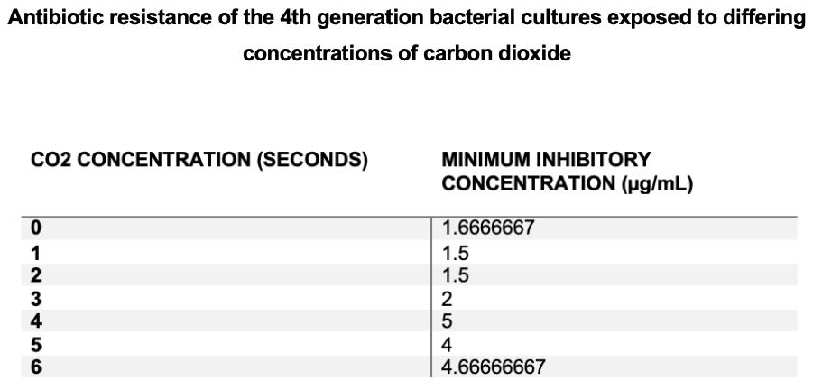
Minimum inhibitory concentration initially decreased in experimental groups exposed to 1 and 2 seconds of CO2 compared to controls, then increased as CO2 concentrations increased. Increased minimum inhibitory concentrations were seen at higher CO2 concentrations (4, 5 and 6 seconds) in comparison to that of control cultures, indicating that bacterial cultures exposed to increased CO2 concentrations possessed more antibiotic resistance. Highest Minimum inhibitory concentrations were expressed in 4 second cultures indicating that this group was the most resistant.
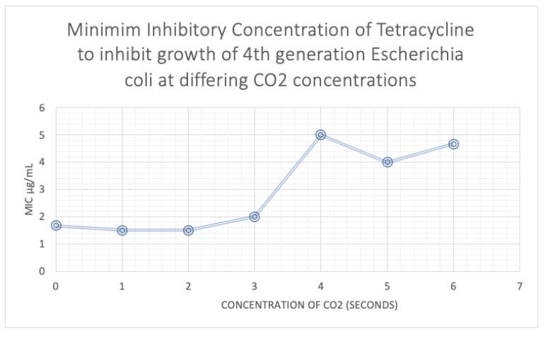
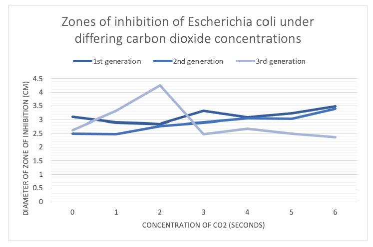 Figure 1a) – Average zones of inhibition of each experimental group were measured at bacterial generation 1, 2, and 3.
Figure 1b) – Average zones of inhibition of each experimental group were graphed at bacterial generation 1, 2, and 3.
Figure 2a) – Average minimum inhibitory concentration of each experimental group was measured at bacterial generation 4 through e-test strips.
Figure 2b) – Average MICs of each experimental group at bacterial generation 4 were tabulated.
Figure 1a) – Average zones of inhibition of each experimental group were measured at bacterial generation 1, 2, and 3.
Figure 1b) – Average zones of inhibition of each experimental group were graphed at bacterial generation 1, 2, and 3.
Figure 2a) – Average minimum inhibitory concentration of each experimental group was measured at bacterial generation 4 through e-test strips.
Figure 2b) – Average MICs of each experimental group at bacterial generation 4 were tabulated.
The Journal of Science Extension Research – Vol. 1, 2022 education.nsw.edu.au 39
Figure 3a) – Rate of change between the 1st and 3rd bacterial generation was calculated through subtracting zones of inhibition of the 3rd generation from the 1st generation zones of inhibition.
Statistical analysis of the 3rd generation minimum inhibitory concentrations between the control and the 6 second CO2 experimental groups (see appendix I)
Figure 3b) – Rate of change of antibiotic resistance of each experimental group between the 1st and 3rd bacterial generation was tabulated
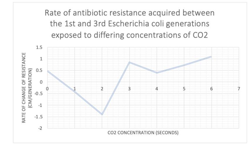
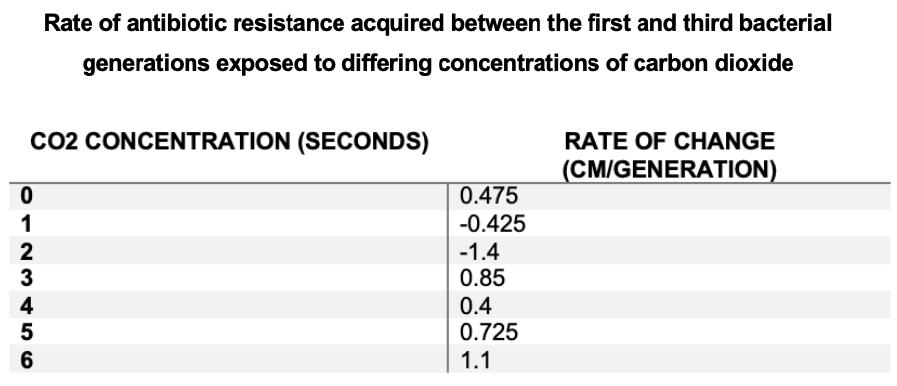
The rate of antibiotic resistance initially decreased, whereby both 1 and 2 second experimental groups possessed negative rates of change between the first and the third generations, whereby the first generations of these 2 experimental groups possessed smaller zones of inhibition and were more resistant than the third generation of these same groups as shown in Figure 1a) and 1b). The rate then increased as concentration increased, whereby the 6 second experimental group had the greatest rate of resistance acquired between the 1st and 3rd bacterial generations.
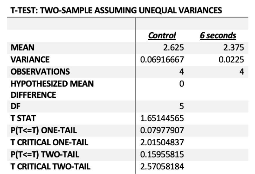
The relationship between the average zones of inhibition of the control and 6 second experimental groups in the third generation was not statistically significant as P=0.16, whereby there is more than a 5% chance that the results were due to chance. Therefore, carbon dioxide had no significant effect on the degree of antibiotic resistance acquired by the third generation bacteria.
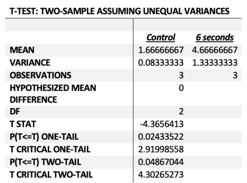
Statistical analysis of the 4th generation minimum inhibitory concentrations between the control and the 6 second CO2 experimental groups
Figure 4 - P(T<=t) two-tail = 0.16 (P> 0.05)
The Journal of Science Extension Research – Vol. 1, 2022 education.nsw.edu.au 40
Figure 5 - P(T<=t) two-tail = 0.04 (P< 0.05)
The relationship between the average zones of inhibition of the control and 6 second experimental groups in the fourth generation was statistically significant as P=0.04, thus there is a less than 5% chance that the results were due to chance. Therefore, carbon dioxide affected the degree of antibiotic resistance acquired by the fourth generation, whereby Figure 2a) and 2b) indicate that increased carbon dioxide increased the degree of antibiotic resistance.
Statistical analysis of the rate of resistance between the control and 6 second CO2 experimental groups acquired between the 1st and 3rd bacterial generations
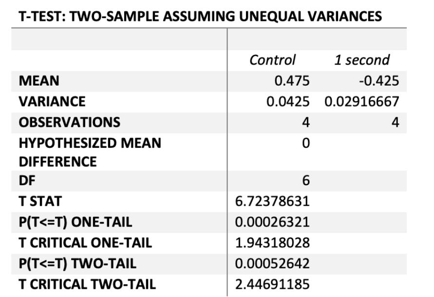
Statistical analysis of the rate of resistance between the control and 1 second and 2 second CO2 groups acquired from the 1st to the 3rd bacterial generation
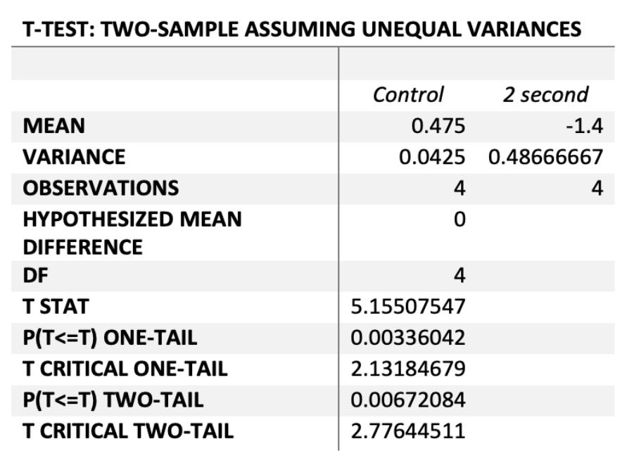
The relationship between the average rate of resistance of the control and 6 second group acquired between the 1st and 3rd generation was statistically significant at P=0.0079, thus there is a less than 1% chance that the results were due to chance. Therefore, increased carbon dioxide significantly increased the rate that antibiotic resistance was acquired between the 1st and 3rd bacterial generations.
The rate of resistance between the control and the low concentrations of CO2 were statistically significant, whereby both the 1 and 2 second experimental groups had significantly lower rates of change than control cultures at P=0.0005 and P=0.007 respectively. Thus the rate of antibiotic resistance in these 2 experimental groups was significantly decreased due to low CO2 concentrations compared to the controls.
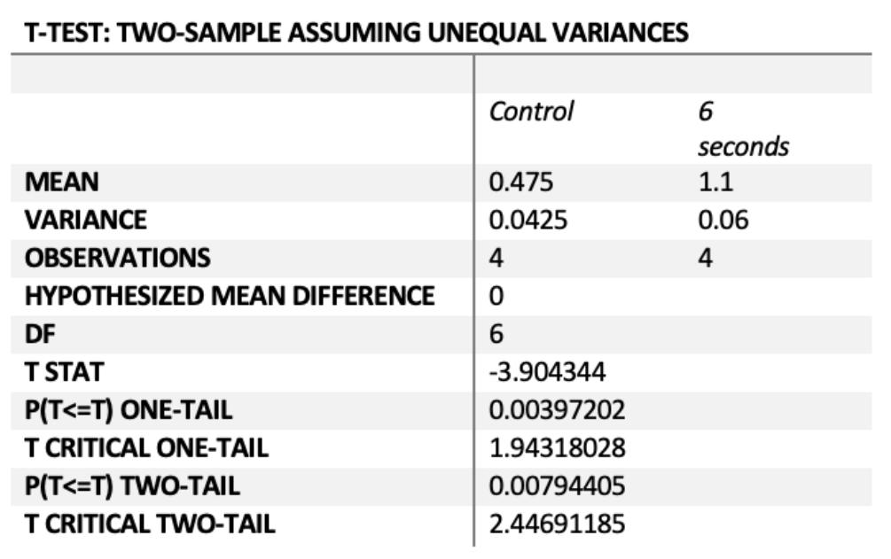 Figure 6 - P(T<=t) two-tail = 0.0079 (P< 0.05)
Figure 7a) – P(T<=t) two-tail = 0.0005 (P<0.05)
Figure 7b) – P(T<=t) two-tail = 0.0067 (P<0.05)
Figure 6 - P(T<=t) two-tail = 0.0079 (P< 0.05)
Figure 7a) – P(T<=t) two-tail = 0.0005 (P<0.05)
Figure 7b) – P(T<=t) two-tail = 0.0067 (P<0.05)
The Journal of Science Extension Research – Vol. 1, 2022 education.nsw.edu.au 41
DISCUSSION
The T-tests conducted between controls and the 6 second CO2 group (see Figure 5) found significantly increased resistance of fourth generation Escherichia coli as P<0.05 and in addition found that the rate of resistance acquired by the 6 second CO2 group between the 1st and 3rd generation was significantly affected by increased CO2 concentrations as P<0.05 (see figure 6). Therefore, the null hypothesis that increasing concentrations of carbon dioxide will have no effect on the extent of antibiotic resistance acquired by E.coli will be rejected in favour of the alternate hypothesis. The P values found suggest that there is less than a 5% chance that the null was incorrectly rejected in a type 1 error.
In both the first and second bacterial generations, zones of inhibition increased as CO2 concentration increased, whereby it was deduced that increased carbon dioxide exposure in the first and second bacterial generations resulted in decreased antibiotic resistance of E.coli in comparison to the control group (see figure 1a and 1b).
Third generation zones of inhibition decreased in increased CO2 concentrations compared to the control, however this was not statistically significant, as P>0.05 for experimental groups in comparison to the control group (see figure 4). Third generation zones of inhibition increased initially in the 1 and 2 second groups in comparison to the control group before decreasing over the 3, 4, 5 and 6 second experimental groups (see figure 1a and 1b). This supports studies relating to the ability for E.coli to become adapted to CO2, initiating CO2 mutations that are dependent on high
concentrations of CO2 and cannot be initiated effectively under ambient air (Charles & Roberts, 1968; Ueda et al., 2008). The lower concentrations of CO2 in the 1 and 2 second groups may not be high enough to induce these mutations, however warrants further investigation to investigate the reliability of the results and a link between CO2 mutations and antibiotic resistance. The bacterial cultures exposed to 6 seconds of CO2 expressed the largest degree of resistance in the third generation with 2.375cm diameter zones of inhibition on average compared to 2.625cm of the controls (see figure 1a), which was not statistically significant, however the trend shown in figure 1b) suggests that increased CO2 may result in increased antibiotic resistance.
In the fourth generation, antibiotic resistance was quantified through minimum inhibitory concentrations (MICs). MIC increased as CO2 concentration increased, which validated the generation 3 results (see figure 2a and 2b). The MICs of the 6 second CO2 acterial cultures were significantly higher than the control group, where P=0.04 (see figure 5) thus suggesting that increased CO2 concentration may result in increased antibiotic resistance.
Considering that the resistance of the third generation 6 second CO2 bacteria was not statistically significant in comparison to controls at P=0.16, (see figure 4) the significance of the fourth generation suggests that the effect of CO2 on antibiotic resistance may increase with each generation due to the phenotypic changes of biological variation, requiring further investigation with additional bacterial generations.
The Journal of Science Extension Research – Vol. 1, 2022 education.nsw.edu.au 42
The contrasting decrease in antibiotic resistance as CO2 concentrations increased in generations 1 and 2 (see figure 1a and 1b) raises questions about whether CO2 initially acts as a negative selection pressure for the bacteria’s survival, enabling a faster rate of resistance in future generations due to adaptation. This is supported by Santillan et al. (2015) in the isolation of a CO2 tolerant Lactobacillus strain, whereby high aqueous CO2 concentrations initially stressed the population before creating a niche for adapted CO2 tolerant bacteria. Further investigation is therefore required pertaining to the nature of the continued rate of survival of Escherichia coli exposed to CO2 without antibiotics.
It’s also worth noting that although the fourth generation bacteria exposed to 6 seconds of CO2 were significantly more resistant in comparison to the fourth generation control group (see figure 5), the MIC of the 6 second group (with the greatest extent of resistance within the study) indicated that the bacteria were not clinically resistant in conjunction with the CLSI guidelines (see appendix J), whereby the MIC must be greater than or equal to 16 μg/mL for the bacteria to be considered resistant (Weinstein et al., 2020). Since the average MIC of the 6 second experimental group was 4.67 μg/mL (see Figure 2a), these bacteria are considered to be between clinically susceptible and intermediate (Weinstein et al., 2020). Thus, in this study, CO2 had a significant impact on the resistance acquired by the bacteria in comparison to the controls, but it would not indicate major problems with the effectiveness of antibiotic treatments. Further research is required to determine if this would change with additional bacterial generations or a larger sample size.
It was also found that increased CO2 concentrations resulted in an increased rate of resistance acquired between the first and third generation of the 6 second experimental group compared to the controls where P=0.08 (see figure 6). This increased rate of resistance (see figure 3a and 3b)may be a result of the increased dissemination of antibiotic resistance genes when exposed to high concentrations of CO2 (Liao et al., 2019). It was also found that bacteria in the 1 and 2 second groups had significant negative rates of change in comparison to the controls where P=0.0005 and P=0.006 respectively, whereby the antibiotic resistance decreased from the 1st to the 3rd generation (see figure 7a and 7b). This may be a result of the CO2 concentrations being too low to induce CO2 mutations of bacteria (Charles & Roberts, 1968), however a larger sample size and further investigation of a link between CO2 mutations and antibiotic resistance is required
The significant increase in extent of resistance of the 6 second CO2 cultures compared to the controls in the 4th generation suggests that projected increases in atmospheric carbon dioxide concentration may potentially result in widespread increases in antibiotic resistance. Furthermore, the significance of the increased rate of resistance between the control and the 6 second groups supports research by Liao et al. (2019) pertaining to an increase in the dissemination of ARGs when exposed to increased CO2 concentrations that result in faster acquisition of antibiotic resistance. Despite the fact that no bacteria in this study were classified as being clinically resistant by CLSI guidelines, the trends model the potential contribution of CO2 to the development of
The Journal of Science Extension Research – Vol. 1, 2022 education.nsw.edu.au 43
antibiotic resistance, which may increase burdens on public health as CO2 emissions continue to increase. Replication is required to verify this relationship on a larger scale, with further bacterial generations as well as supporting investigations to determine thresholds for CO2 tolerance, CO2 as a negative selection pressure for bacteria and the occurrence of this phenomenon in other bacteria such as Staphylococcus aureus, which is known to become readily resistant to a wide variety of antibiotics (Chambers & DeLeo, 2009).
LIMITATIONS
The small sample size of each group (n=4 cultures), limits the reliability of the trends relating to the exposure of CO2 and antibiotic resistance. A larger sample size would be beneficial in drawing more reliable relationships between carbon dioxide and antibiotic resistance in each experimental group through the ability to assess consistency of results. The Ttests, although able to compare the average resistance of the controls and each experimental group, was limited by the sample size, so the statistical significance of the data may be less accurate and reliable, therefore the statistical significance in this study may not apply to a larger population. Furthermore, the lack of repetition due to time and resource constraints means that the results of this investigation are not reliable. Future investigations should be repeated to obtain multiple results, to ensure the results are consistent and thus reliable.
The validity of the investigation may have been impacted through the utilisation of e-test strips to obtain MIC values in the fourth generation, as compared to
measuring zones of inhibition to quantify antibiotic resistance in the first to third bacterial generations. MIC values were used in the 4th generation to validate the results of the 3rd generation and determine if the bacteria were clinically resistant, however the ability to compare the third and fourth generations is limited due to different measurement methods and further investigation examining the progression of antibiotic resistance through additional bacterial generations is necessary with the use of consistent measurement methods.
The lack of appropriate equipment may have hindered the validity and accuracy of the investigation, particularly the lack of a carbon dioxide incubator and the inability to incubate cultures in known and sustained carbon dioxide environments, whereby a CO2 incubator was used to ensure a constant environment of 5% CO2 in a study conducted by Ueda et al. (2008). Despite constructed airtight seals, it is possible that the environment was not able to be kept constant, limiting the controlled variables and thus the validity and accuracy of the results in each experimental group (see appendix B). Furthermore, the inability to quantify the concentration of CO2 inhibits comparison of results against current and projected atmospheric concentrations.
CONCLUSION
Findings indicate a link between carbon dioxide exposure and antibiotic resistance acquired by Escherichia coli over 4 generations, as it was found that increased carbon dioxide exposure resulted in significantly increased antibiotic resistance of 4th generation
E.coli. Thus the null hypothesis was rejected in favour of the alternate
The Journal of Science Extension Research – Vol. 1, 2022 education.nsw.edu.au 44
hypothesis, through the significant increase in resistance of the 6 second group compared to the control in the 4th generation (P=0.04), and an increased rate of resistance of this group acquired throughout the 1st to 3rd generations (P=0.008). This suggests that projected increases in global atmospheric carbon dioxide concentrations could potentially contribute to increases in the rate and extent of antibiotic resistance which could have large consequences on public health in the ability to treat infectious disease. Further investigation is required to ensure the reliability of this link through repetition of this experimental method, and could be further extended to test other bacterial species, for example Staphylococcus aureus, which is known to become readily resistant to a wide variety of antibiotics (Chambers & DeLeo, 2009).
ACKNOWLEDGEMENTS
I would like to thank my teacher Ms. Ann Hanna for obtaining equipment, supervising and assisting with logistics, as well as my mentor Amy Sarker from the University of Sydney for helping with alternate solutions for equipment and data collection. I would also like to express my appreciation to my classmate Rebekah Wood for helping with data collection and for suggestions and feedback regarding the methodology of the investigation, and the Industrial Technology faculty for assisting with equipment.
REFERENCE LIST
Aryal, S. (2018, October 26). Mueller Hinton Agar (MHA) – Composition, Principle, Uses and Preparation.
Microbiology Info.com.
https://microbiologyinfo.com/muellerhintonagar-mha-composition-principleuses-and-preparation/
Bidell, M. R., Opraseuth, M. P., Yoon, M., Mohr, J., & Lodise, T. P. (2017). Effect of prior receipt of antibiotics on the pathogen distribution and antibiotic resistance profile of key Gram-negative pathogens among patients with hospitalonset urinary tract infections. BMC Infectious Diseases, 17(1).
https://doi.org/10.1186/s12879-017-22707
Chambers, H. F., & DeLeo, F. R. (2009). Waves of resistance: Staphylococcus aureus in the antibiotic era. Nature Reviews Microbiology, 7(9), 629–641.
https://doi.org/10.1038/nrmicro2200
Charles, H. P., & Roberts, G. A. (1968). Carbon Dioxide as a Growth Factor for Mutants of Escherichia coli. Journal of General Microbiology, 51(2), 211–224.
https://doi.org/10.1099/00221287-51-2211
Endeward, V., Arias-Hidalgo, M., AlSamir, S., & Gros, G. (2017). CO2 Permeability of Biological Membranes and Role of CO2 Channels. Membranes, 7(4), 61.
https://doi.org/10.3390/membranes70400 61
Ezraty, B., Chabalier, M., Ducret, A., Maisonneuve, E., & Dukan, S. (2011). CO 2 exacerbates oxygen toxicity. EMBO Reports, 12(4), 321–326.
https://doi.org/10.1038/embor.2011.7
Glen, S. (n.d.). Alpha Level (Significance Level): What is it? Statistics How To. Retrieved July 20, 2021, from https://www.statisticshowto.com/probabilit
The Journal of Science Extension Research – Vol. 1, 2022 education.nsw.edu.au 45
y-andstatistics/statistics-definitions/whatis-an-alpha-level/#:~:text=3.-
Hudzicki, J. (2009). Kirby-Bauer Disk Diffusion Susceptibility Test Protocol.
https://asm.org/getattachment/2594ce26bd44-47f6-8287-0657aa9185ad/KirbyBauer-Disk-Diffusion-Susceptibility-TestProtocol-pdf.pdf
Ingham, H. R., Selkon, J. B., Codd, A. A., & Hale, J. H. (1970). The effect of carbon dioxide on the sensitivity of Bacteroides fragilis to certain antibiotics in vitro. Journal of Clinical Pathology, 23(3), 254–258. https://doi.org/10.1136/jcp.23.3.254
Krysan, D. J., Zhai, B., Beattie, S. R., Misel, K. M., Wellington, M., & Lin, X. (2019). Host Carbon Dioxide Concentration Is an Independent Stress for Cryptococcus Neoformans That Affects Virulence and Antifungal Susceptibility. MBio, 10(4).
https://doi.org/10.1128/mbio.01410-19
Latest Cape Grim greenhouse gas data. (2018). Csiro.au; CSIRO.
https://www.csiro.au/en/Research/OandA/ Areas/Assessing-ourclimate/Latestgreenhouse-gas-data
Liao, J., Chen, Y., & Huang, H. (2019). Effects of CO2 on the transformation of antibiotic resistance genes via increasing cell membrane channels. Environmental Pollution, 254, 113045.
https://doi.org/10.1016/j.envpol.2019.113 045
Lindsey, R. (2020, August 14). Climate Change: Atmospheric Carbon Dioxide. Climate.gov; NOAA.
https://www.climate.gov/newsfeatures/understandingclimate/climatechange-atmospheric-carbon-dioxide
Martinez, J. L., & Baquero, F. (2000). Mutation Frequencies and Antibiotic Resistance. Antimicrobial Agents and Chemotherapy, 44(7), 1771–1777.
https://doi.org/10.1128/aac.44.7.17711777.2000
Nunez, C. (2019, May 13). Carbon dioxide levels are at a record high. Here’s what you need to know. National Geographic.
https://www.nationalgeographic.com/envir onment/global-
warming/greenhousegases/#:~:text=Gree nhouse%20gases%20have%20far%2Dra nging
Parker, M. (2009). How to Grow E. Coli in a Petri Dish. Sciencing.
https://sciencing.com/grow-ecoli-petridish-5534225.html
Santillan, E.-F. U., Shanahan, T. M., Omelon, C. R., Major, J. R., & Bennett, P. C. (2015). Isolation and characterization of a CO2-tolerant Lactobacillus strain from Crystal Geyser, Utah, U.S.A. Frontiers in Earth Science, 3.
https://doi.org/10.3389/feart.2015.00041
Ueda, K., Tagami, Y., Kamihara, Y., Shiratori, H., Takano, H., & Beppu, T. (2008). Isolation of Bacteria Whose Growth Is Dependent on High Levels of CO2 and Implications of Their Potential Diversity. Applied and Environmental Microbiology, 74(14), 4535–4538.
https://doi.org/10.1128/AEM.00491-08
Weinstein, M. P., Lewis II, J. S., Bobenchik, A. M., Campeau, S., Cullen, S.K., Galas, M. F., Gold, H., Humphries, R.M., Kirn, Jr, T. J., Limbago, B., Mathers, A. J., Mazzulli, T., Satlin, M., Schuetz, A. N., Simner, P. J., & Tamma, P.D. (2020). M100 Performance Standards for Antimicrobial Susceptibility
The Journal of Science Extension Research – Vol. 1, 2022 education.nsw.edu.au 46
Testing A CLSI supplement for global application. 30th Edition.
https://www.nih.org.pk/wpcontent/uploads/2021/02/CLSI-2020.pdf
Wellington, E. M., Boxall, A. B., Cross, P., Feil, E. J., Gaze, W. H., Hawkey, P. M., Johnson-Rollings, A. S., Jones, D. L., Lee, N. M., Otten, W., Thomas, C. M., & Williams, A. P. (2013). The role of the natural environment in the emergence of antibiotic resistance in Gram-negative bacteria. The Lancet Infectious Diseases, 13(2), 155–165.
https://doi.org/10.1016/S14733099(12)70317-1
APPENDICES APPENDIX A
Aseptic techniques were undertaken throughout the investigation in order to minimise the risk of spreading pathogenic bacteria. This was enabled through the sanitising of all surfaces and equipment before experimentation, between each inoculation, and following completion.
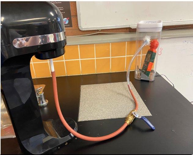
APPENDIX B
Experimental set up as shown with agar plates inside the clear container. This setup was replicated 7 times for each experimental group. A SodaStream with a pressurised CO2 canister was connected to a hose with an on/off tap connected to a hose leading to the airtight container. For each experimental group, agar plates were placed into the corresponding sealed container with the tap on. The SodaStream was turned on for an amount of time denoted by the experimental group, which controlled the amount of CO2 that was pumped into the container.
APPENDIX C
The 7 taps were then turned off and disconnected from the SodaStream at point A. All 7 containers were placed into the same incubator set to 35 degrees Celsius.
A hole was required to be drilled into each container and sealed with silicone. It is possible that this seal did not adequately contain the CO2, limiting the reliability and validity of the data.
turned off and disconnected at point
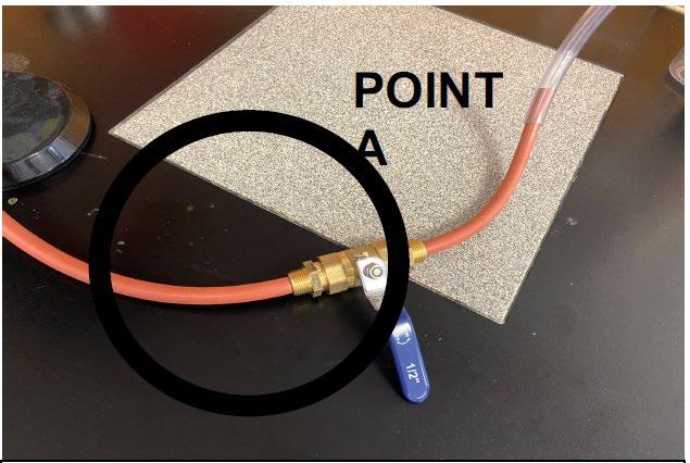
A
Figure B1 – connection point between the SodaStream and the on/off tap. After the gas was pumped into the container the tap was
The Journal of Science Extension Research – Vol. 1, 2022 education.nsw.edu.au 47
Figure B2 – set up for pumping the CO2 into the container. Agar plates were stacked inside the container.
Streptomycin, Sulphatriad and APPENDIX D Tetracycline) was placed into the centre of 4 agar plates. The antibiotic disc with An initial investigation was undertaken in the largest average zone of inhibition was order to determine the appropriate used in this experiment in order to model antibiotic for use throughout the the use of last resort antibiotics that will investigation. 6 Mueller Hinton agar be the most effective in fighting bacterial plates were inoculated with 100 growth. Therefore, the results of the microlitres of Escherichia coli and spread complete investigation represent the to create a bacterial lawn. A mastring, potential public health problem that will containing 5 different antibiotic occur if atmospheric CO2 continues to susceptibility discs (Ampicillin, rise with the most effective antibiotics.
Chloramphenicol, Penicillin G,
Zones of inhibition of E.coli in the presence of differing antibiotics
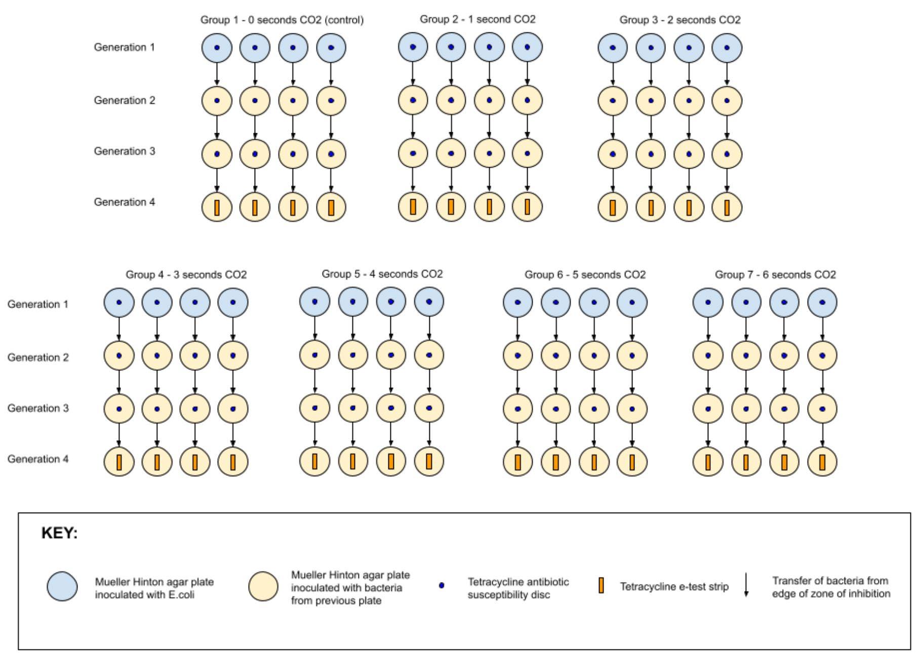 Figure C1 – experiment outline, detailing the transfer of bacteria between each generation within each group.
The Journal of Science Extension Research – Vol. 1, 2022 education.nsw.edu.au 48
Tetracycline was used as the antibiotic with the largest average zone of inhibition as discussed above.
APPENDIX E
Carbon dioxide concentration in each container was quantified through the amount of carbon dioxide pumped into the container using a gas canister with a valve. This measurement was expressed in seconds. Thus, the CO2 was pumped out at a constant rate for each container and pumping was stopped after reaching specific time intervals. The control group was not exposed to additional CO2, however for the group 2 container, CO2 was pumped in for 1 second. CO2 was pumped in for 2 seconds for the group 3 container, 3 seconds for the group 4 container, 4 seconds for the group 5 container, 5 seconds for the group 6 container and 6 seconds for the group 7 container.
APPENDIX F
An inoculating loop was utilised to swab the bacteria at the edges of the zones of inhibition for each culture for each group. Referring to the right image, the bacteria inside the red circle was swabbed and transferred to the corresponding plate.
For example, an inoculating loop swabbed the bacteria that had grown at the edge of the zone of inhibition of a plate from the control group, and this was inoculated onto a plate that would then be part of the control group for this generation.
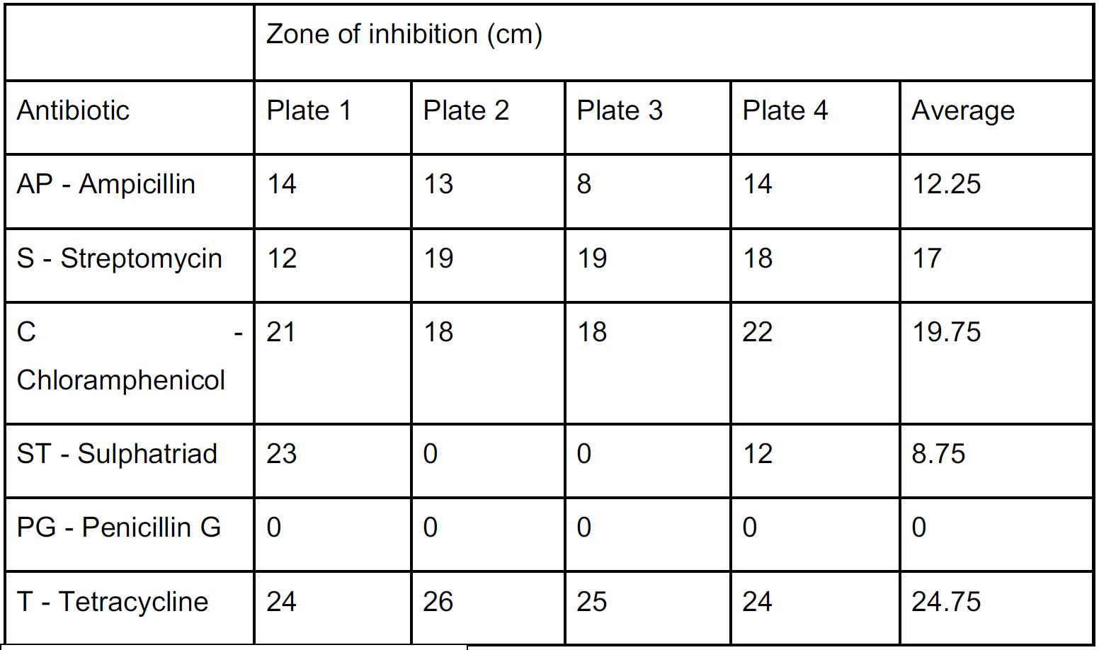 Table D1 – Preliminary investigation results that were used to determine the most suitable antibiotic
The Journal of Science Extension Research – Vol. 1, 2022 education.nsw.edu.au 49
Figure
APPENDIX G
E-test strips (pictured to the right) were used to validate the findings from generation 3, and provide a quantitative value recognised by CLSI guidelines. Larger MICs indicate increased antibiotic resistance.
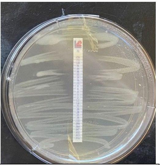
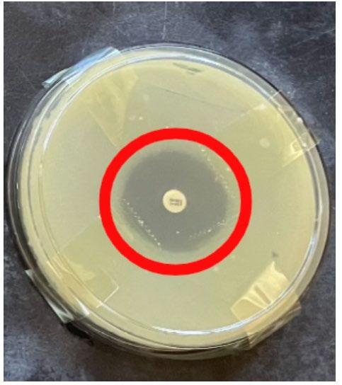
Figure G1 – E-test strips were used in generation 4 to validate generation 3 results and determine the clinical level of resistance through referring to CLSI guidelines
APPENDIX H
T-tests were conducted with an alpha value of 0.05 as a commonly accepted value by scientists to minimise type I and type II errors (Glen, n.d.). Thus obtaining a P value of less than or equal to the alpha is statistically significant.
APPENDIX I
The results of the 3rd generation were statistically analysed due to the validation of their trend in the 4th generation MIC values, and in conjunction with a study conducted by Bidell et al. (2017) that found “two or more prior antibiotic exposures were associated with slightly higher fluoroquinolone nonsusceptibility, multidrug resistance… compared with 0 or 1 exposure”, thus this study required 3 generations at least in order to ensure the bacteria had acquired resistance through 2 previous antibiotic exposures in the 1st and 2nd generations.
APPENDIX J
CLSI guidelines:
F1 – The edges of each zone of inhibition were taken and swabbed onto a new agar plate.
The Journal of Science Extension Research – Vol. 1, 2022 education.nsw.edu.au 50
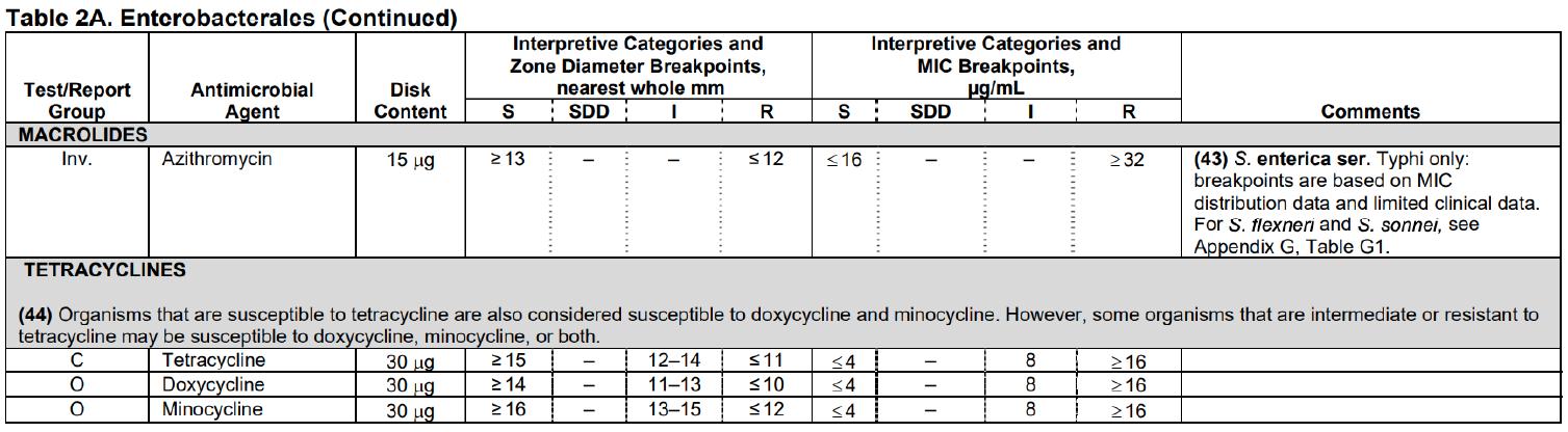
The Journal of Science Extension Research – Vol. 1, 2022 education.nsw.edu.au 51
Table J1 – MIC (μg/mL) of the 4th generation were obtained and connected to the CLSI guidelines to determine if the bacteria were clinically resistant.
Mealworm pupa and the successful survival on a polystyrene diet: the potential for mealworms to reduce the impact of plastics in the environment
Montana Morgan Lambton High School
Observations have been made surrounding the ability of mealworms to successfully digest and break down the polymer polystyrene (PS). Two colonies were established in order to compare the progression of darkling beetle larvae; or mealworms, on a usual oat-diet to a PS-diet. This investigation determined that mealworms are able to successfully mature on a diet predominantly based on expanded polystyrene. Furthermore, results showed that larvae on a PS-diet were able to progress into the pupa and adult, or beetle stage of life at a faster rate than their oat-diet counterparts. This highlights the potential of plastic waste management systems to be implemented that utilise mealworms to degrade potentially harmful plastics.
Literature review:
Polystyrene is a synthetic hydrocarbon polymer discovered by Eduard Simon in 1839 (“Polystyrene,” 2020), which poses significant threats to natural ecosystems due to its ability to withstand biodegradation. The main research area of this investigation was to explore new methods of using invertebrates in the form of mealworms in order to provide a solution to the overwhelming volume of PS waste that reaches natural environments. Despite this research area being relatively new, there are several previous studies which explore different aspects of the topic, allowing for this investigation to produce new data that fills current gaps. The work of Yang and coworkers (2020) suggests that “mealworm[s] (Tenebrio molitor) [where] capable of degrading and mineralizing Styrofoam (PS foam)” (Yang et al., 2020). The 28-day investigation found that
mealworms which were fed styrofoam as a sole diet were able to live just as well as those fed on a usual diet of oat bran. The study also concluded that the average PS foam consumption rate was 0.14 mg/d, suggeting that this method may be feasible to introduce on a larger scale. Another investigation led by Hughes (“Teens Use Science to Worm through Plastic Waste,” 2016), aimed to discover which type of plastic mealworms could most efficiently digest. The investigation involved feeding mealworms small amounts of Polyethylene terephthalate (PET), polyethylene (PE), Polystyrene (PS) and Polypropylene (PP) sourced from conventional plastic waste. The experiment concluded that the mealworms consumed 64% of the PS, 50% of the PET, 40% of the PP and 29% of the PE. Hughes' experiment is beneficial as it identifies PS as the polymer that mealworms most readily consume, and provided a basis for this
The Journal of Science Extension Research – Vol. 1, 2022 education.nsw.edu.au 52
investigation to focus on a single plastic type, although the article may have reduced reliability as it is not from a peerreviewed academic source. A third article by Siva (2020), furthered the research area through identifying the types of microbes present within the mealworm's gut that are able to digest PS. The article acknowledges the severity of PS pollution within the environment, stating that an “An estimated 359 million tons of plastic [was] produced globally in 2018, including 33 million tons of polystyrene” (Beetle Larvae Can Survive on Polystyrene Alone, n.d.). It is also speculated that the mealworm's ability to biodegrade plastics is evolutionary-based. This is due to scavengers, such as mealworms, consuming lignin (wood-based substances) for food, which is highly difficult to break down as lignin is a complex biopolymer that is both hydrophilic and insoluble to most solvents (Lignin - an Overview | ScienceDirect Topics, n.d.). The researchers stated that they were beginning to isolate certain gut bacteria within the mealworms to test their ability to degrade plastic (Beetle Larvae Can Survive on Polystyrene Alone, n.d.). However, this study did not investigate the effectiveness of a PS diet in terms of the mealworm's ability to develop past larvae stage, highlighting the gap that was explored in this investigation.
The ability of invertebrates to successfully digest plastics is not limited to mealworms, with other insect larvae being capable of surviving on a PS diet. For example, Billen and coworkers (2020) observed larvae of the greater wax moth (Galleria mellonella), which seemed to chew and digest polyethylene; although whether they successfully degraded the polyethylene was unknown. This
investigation aimed at understanding the mechanisms behind the wax moth’s gut microbes and how it can be applied to technology in order to replicate it in a more efficient manner. This is due to 4-10 tonnes of greater wax moth larvae being needed to digest 1 tonne of plastic (Billen et al., 2020). Such research showed the need for an invertebrate that will be more efficient in digesting plastic, in comparison to wax moths, to make a large-scale replication feasible. This notion leads to Rodrigues’ investigation (2016), which compared the plasticdigesting ability of mealworms to superworms (Zophobas morio). The three week comparative experiment concluded that mealworms largely outperform superworms; with 5 mealworms consuming 1 gram of plastic in two days, which is more than what the superworms could consume in a week (“Teens Use Science to Worm through Plastic Waste,” 2016). Another benefit for the use of mealworms as a method for polystyrene waste control is their existing use as a common food source for other species including a range of birds, reptiles and fish in the agricultural and pet industries. The investigation highlighted the ability of mealworms to consume relatively high quantities of PS in comparison to other invertebrates, indicating that along with their availability, they were the ideal choice for an invertebrate in this investigation.
The possible implications of these findings has also been acknowledged, with the prospect to create a zero-waste sustainable bioremediation cycle. Another study from 2020 highlights the possibility of using mealworms as a source to degrade PS, while also utilising the frass to assist in the growth of plants, specifically dragon fruit cacti (Koh et al.,
The Journal of Science Extension Research – Vol. 1, 2022 education.nsw.edu.au 53
2020). The study also researched which supplement was best for promoting PS consumption. Three different supplements were studied: bran, cinnamon and table sucrose, with the mealworms mass being calculated after 4 days. Results; shown in figure 2, determined that table sucrose and bran almost doubled the PS consumption from the control, with the consumption rate rising from 1.035 and 1.397 mg / g of worm per day to 1.787 and 2.142, respectively (Koh et al., 2020). The study demonstrated the possibility of a practical application to reduce PS waste entering the natural environment. The question of the possible risk of biomagnification arose, as PS commonly contains pollutants and additives including UV stabilisers, antioxidants and flame
retardants (Smith & Taylor, 2002). Furthermore, Browne and coworkers (2013) demonstrated the minimal influence of microplastics on the transfer of pollutants into the tissue of lugworms, a close relative of mealworms. The study found that biochemically clean sand transfers more pollutants into the worm’s tissue than microplastics (Browne et al., 2013). Thus, the potential of mealworms to become an efficient method of PS control, alongside the minimal risk of biomagnification showed strong merit in further research being completed within this area as well as prototype methods being constructed to determine the viability of mealworms being used as a means of polystyrene control.
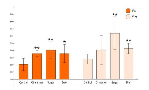
The Journal of Science Extension Research – Vol. 1, 2022 education.nsw.edu.au 54
Figure 1: Average rate of PS consumption (mg / g of worm per day) by superworms (Sw) and mealworms (Mw) with and without food additives (cinnamon, sugar and bran(Koh et al., 2020)
Scientific research question:
To what extent are mealworms able to consume and successfully develop on a diet predominantly based on polystyrene, examining the effect of altered diet on:
• Mean larvae body mass
• Mortality during larvae and pupa stage
• Number of successful maturing adults
Hypothesis:
Null Hypothesis: mealworms on a diet predominantly consisting of polystyrene will be unable to maintain their body mass and therefore not successfully develop into the pupa or eventual adult stage of their life cycle.
Alternative hypothesis: mealworms on a diet predominantly consisting of polystyrene will be able to maintain their body mass and successfully develop into the pupa and eventual adult stage of their life cycle.
Methodology:
Prior to the commencement of the methodology, an ethical report (see Appendix 1) was prepared in order to ensure all considerations including sourcing mealworms and their disposal are successfully met.
Required materials:
Consumables:
• 2000 Mealworms - sourced from Petstock
• Potato - sourced from Coles
• Oatbran (ground rolled oats)sources from Coles
• Polystyrene (disposable cups ground styrofoam) - sourced from Coles.
Non-consumables:
• 3x four draw storage cabinetssourced from Office Works
• 8x small plastic containers (chinese take away containers)
• Scales
• Ruler
• Blender
• Sieve
• Knife
• Metal tweezers
• Beakers
Colony establishment:
The Methodology accepted to investigate the hypothesis involves creating two colonies of mealworms to compare data. One colony acted as a control, consisting of four sets of approximately 250 mealworms being fed a diet of ground oats (oat-diet) alongside a slice of potato for moisture and trace nutrients. The other colony will consist of the same number of mealworms and slices of potato, but were fed shredded polystyrene (PS-diet) in replacement of an oat-diet. These colonies were maintained within storage draws (as shown in figure 2) with holes drilled along the top to ensure airflow. Each draw was filled with 3-4cm of ground oats or shredded PS for the control and experimental colony respectively.
The Journal of Science Extension Research – Vol. 1, 2022 education.nsw.edu.au 55
Data collection methodology:
At the beginning of the investigation, the mass of a random sample of 20 larvae was recorded. The colonies were maintained and monitored for 28 days; which is the approximate time mealworms are in larvae stage(Instructions on Breeding Mealworms, n.d.), by regularly measuring the mass of a random sample of 20 larvae and recording any larvae that progressed to the pupae stage. Throughout the experiment, any larvae or pupa deaths were recorded to provide a measure of the survival of the mealworms. Any surviving mealworms that made it to the adult stage of their life cycle were tallied and separated into 8 small plastic containers (4 PS-diet and 4 Oat-diet) with the intention of establishing additional colonies for potential future research into the impact of a PS-diet on subsequent mealworm generations. The decision to have four sets of approximately 250 mealworms within each colony was chosen to have a
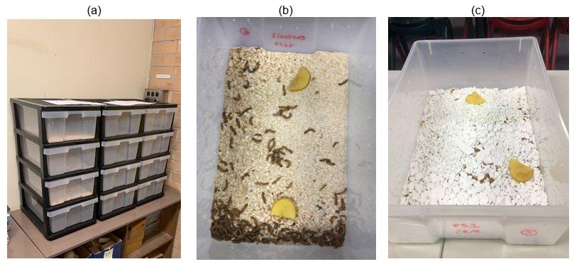
sufficiently large colony population to reduce the impact of environmental and observational random error when only sampling a relatively small portion of the population.
Data analysis methodology:
Once this data was collected, a range of techniques were utilised in order to complete a statistical analysis. As the data being collected is primary and quantitative, descriptive statistics such as mean, median and standard deviation were calculated. These measurements are represented graphically in order to highlight trends and patterns present within the data. This statistical data was found for both the control and experimental colony, allowing for a comparison between the two data sets via a two tailed t-test to examine whether the observed differences in the mean body mass of the colonies were statistically significant.
Figure 2: colony set up of (a) 3 sets of draws for 2 colonies and spares for adults & trials (b) oat-diet draw and (c) PS-diet draw
The Journal of Science Extension Research – Vol. 1, 2022 education.nsw.edu.au 56
Results:
Effect of altered diet on mean larvae body mass:
The observed body mass of the control (oat-diet) and test (PS-diet) colony tracked over the 28-day period of the study is shown in Table 1. Figure 3 shows the observed trend in the mean sampled body mass throughout the 28-day trial. The lines of best fit for each colony clearly show that the mean sampled body mass of the PS-diet colony is comparable across the period of the study with a slight decline in body mass becoming evident after day 10. A two tailed t-test
assuming equal variances with an alpha value of 0.05 (Table 2) showed that the test colony on the PS-diet (M= 52, SD= 3.5) compared to the control colony on the oat-diet (M= 54 , SD= 3.1) was observed to have a statistically significantly different mean body mass across the 28-day study period, t(2.7)= 2.0, p= 0.009. As the p value is smaller than the alpha value, the null working hypothesis was able to be rejected, stating that the mean body mass of the control colony is equal to the test colony. This presents strong evidence that the observed differences in the mean body mass between each mealworm colony is considerable.
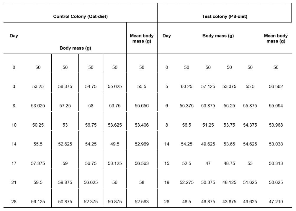
The Journal of Science Extension Research – Vol. 1, 2022 education.nsw.edu.au 57
Table 1: observed body mass over 28 days based on a random sample of 20 mealworms.
Figure 3: approximate change of mass of mealworm larvae over a 28-day period based on a sample size of 20
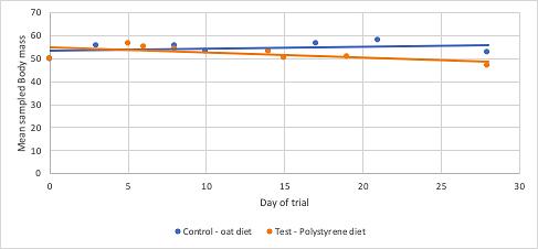
Table 2: Summary statistics for the two tailed t-test assuming equal variances with an alpha value of 0.05 comparing mean body mass of the test colony on the PS-diet to the control colony on the oat-diet. (Null hypothesis: mean mass of PS MW = mean mass of oatm
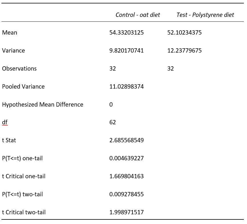
The Journal of Science Extension Research – Vol. 1, 2022 education.nsw.edu.au 58
Effect of altered diet on mortality during larvae stage:
Throughout the investigation, the number of mealworm larvae was collected, with the cumulative mortality for the combined 4 trials of the oat-diet and PS-diet colonies being displayed in figure 4. In relation to the control colony, there is a strong positive correlation between the cumulative mortality and time throughout the 28-day trial. This determines that the number of larvae mortality was consistent and above zero during the investigation.
In contrast, the PS-diet colony is shown to have a smaller cumulative larvae mortality in comparison to the control colony, alongside increasing in cumulative mortality past the 15th day of the investigation. As well as this, the first larvae found dead within the polystyrene colony was earlier than the first found dead within the control colony. The control colony has a mortality rate of 5.6 deaths per 100 larvae, in comparison to a mortality rate of only 0.5 deaths per 100 larvae for the polystyrene colony. This poses strong evidence for mealworms to successfully mature on a PS-based diet.
Effect of altered diet on number of successful maturing adults:
Figure 5 shows the cumulative number of successful pupa formed from larvae throughout the 28 day trial. A significant trend shown within figure 5 is that the Polystyrene colony began to form into pupa two days prior to when the control colony first progressed into pupa. As a
result of this, at day 28 of the trial, the PS-diet colony had 696 larvae that had become pupa, whereas only 603 pupa were formed during this time within the oat-diet colony. Furthermore, Table 3 depicts the cumulative number of beetles formed within each colony, collating the data from the four replicates of each colony. It is shown that throughout the 28 days, the polystyrene colony produced
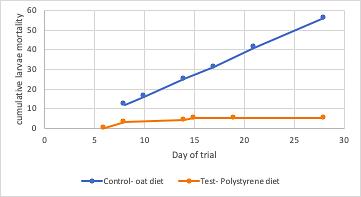 Figure 4: graph showing cumulative larvae mortality of both control and test colony over 28 day period
The Journal of Science Extension Research – Vol. 1, 2022 education.nsw.edu.au 59
more beetles, or adult mealworms, in comparison to the control. This shows that under a polystyrene diet, mealworms
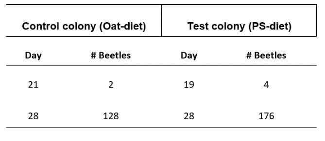
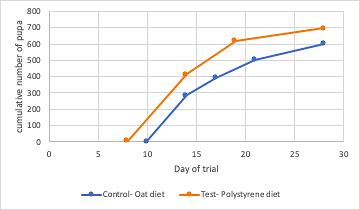
may be able to more efficiently mature into successful adults in comparison to the control, oat-diet.
Discussion:
The impacts of plastic waste on the natural environment are becoming increasingly apparent; with a significant proportion of this waste being polystyrene. Manufacturing and households produced 38.4 and 14.5 thousand tonnes of PS waste respectively within Australia over 2016-17 (Waste Account, Australia, Experimental Estimates, 2016-17 Financial Year |
Australian Bureau of Statistics, 2019). This has resulted in an increasing amount of PS entering waste streams each year, ultimately leading to a high risk of PS entering the natural environment. PS waste that enters the environment has been linked to numerous detrimental effects, including chemical leaching, bioaccumulation, alongside a potential choking hazard for wildlife if broken down (Kik et al., 2020). The significant impact of PS on the natural environment is a driving force for this research.
Figure 5: graph showing cumulative pupa of control and test colony over 28 day period
Table 3: cumulative number of beetles observed over the 28 day study period.
The Journal of Science Extension Research – Vol. 1, 2022 education.nsw.edu.au 60
The findings of this investigation successfully indicates the potential for mealworms to break down polystyrene while surviving to maturity; thus reducing the negative impacts of plastics on the environment. This confirms the claim that mealworms are capable of consuming polystyrene posed by Hughes (“Teens Use Science to Worm through Plastic Waste,” 2016). The small amount of potato used for moisture and trace nutrients within this investigation was unlikely to provide a significant source of nutrition for the mealworms on the PSdiet, meaning that they are consuming the polystyrene to maintain their body mass and progress through their lifecycle. This could be confirmed within future investigations by using a damp cotton ball in place of potato slices to avoid providing a secondary food source. Although this aspect of the methodology may reduce the confidence of the conclusions, the results still provide strong evidence that the larvae are capable of maturing on this altered diet. These findings are also consistent with the work of Yang and coworkers (Yang et al., 2020), which similarly determined that mealworm larvae are able to survive on a diet of PS. The same 28-day period trial and control material leading to similar results within both experiments highlights the reliability and validity of this investigation. However, this investigation also raises several new research questions surrounding the apparent increased rate of progression through the life cycle of mealworms in the colony on a PS-diet in comparison to the colony on an Oat-diet. This is consistent with the qualitative observations of the PS-colony larvae being more physically active in comparison to larvae in the oatdiet colony. This may also be a potential selection pressure that could be used to
explore the effect of the PS-diet on the microbes within the larvaes GI tract in a future investigation, possibly expanding on the work presented by Siva (2020)(Beetle Larvae Can Survive on Polystyrene Alone, n.d.). Another aspect of the methodology that may impact the results of the investigation is the size of the PS used within the PS-diet colony. The styrofoam cups used in the PS colony are significantly less dense than the mealworms, leading to most larvae settling to the bottom of the containers. This made the process of counting individuals that had moved onto the pupa stage or any mortalities much harder to complete compared to the oat-diet, which remained on the surface of the bedding. This aspect may impede on an accurate reflection of the mortality experienced in the PS-diet colony. However, altering materials to use polystyrene blended more thoroughly into a finer particle size may help avoid this.
Future directions of study available for this investigation include a multigenerational approach, by which the offspring of the PS-diet are raised under the same conditions to determine the long-term implications of the altered diet. This leads to investigations surrounding the functionality of the colony, to determine if the offspring can also live off PS or if a new batch of mealworms has to be introduced in place of each new generation. As well as this, additional research could be placed on the impact of certain additives on the consumption rate of PS, first explored by Koh and coworkers (Koh et al., 2020). A wide variety of additives can be investigated, including cinnamon and table sucrose used within the previous study. This information will be of high value if waste
The Journal of Science Extension Research – Vol. 1, 2022 education.nsw.edu.au 61
management strategies were to be put in place in order to ensure the efficiency of polystyrene consumption. Furthermore, a real-world simulation could be constructed using waste PS as a food source; instead of an artificial trial, to provide insight into the possibility of mealworms being implemented into areas such as landfills in order to control the plastic waste that may end up in surrounding ecosystems.
Conclusion:
This investigation confidently shows the potential for mealworms to reduce the impact of plastics on the environment. The investigation involved the establishment of two colonies; PS-diet and oat-diet, to compare their ability to successfully mature into adults. It was found that there was a significant statistical difference between the mean body mass of the PS-diet and oat-diet colonies, alongside the establishment of the trend that the PS-diet colony progressed to the pupa and beetle life stages before the control colony. This allowed for the null hypothesis to be rejected, and provides strong evidence in support of the alternative hypothesis. The investigation's findings also highlight several opportunities for further research to be conducted surrounding both multigenerational colonies and the conformation of life stages occurring quicker; alongside the completion of a real-world investigation to determine the plausibility of using mealworms as part of a waste management scheme. Overall, this investigation provided clear evidence that mealworms have the ability to successfully live off a PS-based diet, giving value to the notion that invertebrates could be employed as part of a waste management system in order
to combat plastic waste entering natural environments.
Acknowledgements:
I would like to thank Mr Nicholson for his valuable assistance and guidance throughout all stages of the investigation and report.
Reference List:
Beetle Larvae Can Survive on Polystyrene Alone. (n.d.). The Scientist Magazine®. Retrieved November 26, 2020, from https://www.thescientist.com/news-opinion/beetle-larvaecan-survive-on-polystyrene-alone-67251
Billen, P., Khalifa, L., Van Gerven, F., Tavernier, S., & Spatari, S. (2020). Technological application potential of polyethylene and polystyrene biodegradation by macro-organisms such as mealworms and wax moth larvae. Science of The Total Environment, 735, 139521.
https://doi.org/10.1016/j.scitotenv.2020.13 9521
Browne, M. A., Niven, S. J., Galloway, T. S., Rowland, S. J., & Thompson, R. C. (2013). Microplastic Moves Pollutants and Additives to Worms, Reducing Functions Linked to Health and Biodiversity. Current Biology, 23(23), 2388–2392.
https://doi.org/10.1016/j.cub.2013.10.012
Instructions on Breeding Mealworms (n.d.). Exotic Nutrition. Retrieved August 18, 2021, from https://www.exoticnutrition.com/how-toraise-mealworms.aspx
Kik, K., Bukowska, B., & Sicińska, P. (2020). Polystyrene nanoparticles: Sources, occurrence in the environment,
The Journal of Science Extension Research – Vol. 1, 2022 education.nsw.edu.au 62
distribution in tissues, accumulation and toxicity to various organisms.
Environmental Pollution, 262, 114297.
https://doi.org/10.1016/j.envpol.2020.114 297
Koh, D. W.-S., Ang, B. Y.-X., Yeo, J. Y., Xing, Z., & Gan, S. K.-E. (2020). Plastic agriculture using worms: Augmenting polystyrene consumption and using frass for plant growth towards a zero-waste circular economy. BioRxiv, 2020.05.29.123521.
https://doi.org/10.1101/2020.05.29.12352
Lignin An overview | ScienceDirect Topics. (n.d.). Retrieved June 26, 2021, from
https://www.sciencedirect.com/topics/mat erials-science/lignin
Polystyrene. (2020). In Wikipedia
https://en.wikipedia.org/w/index.php?title= Polystyrene&oldid=990125404
Smith, S. H., & Taylor, L. T. (2002). Extraction of various additives from polystyrene and their subsequent analysis. Chromatographia, 56(3), 165–169. https://doi.org/10.1007/BF02493206
Teens use science to worm through plastic waste. (2016, June 21). Science News for Students.
https://www.sciencenewsforstudents.org/ article/teens-use-science-worm-throughplastic-waste
Waste Account, Australia, Experimental Estimates, 2016-17 financial year | Australian Bureau of Statistics. (2019, September 18).
https://www.abs.gov.au/statistics/environ ment/environmental-management/waste-
account-australia-experimentalestimates/2016-17
Yang, Y., Wang, J., & Xia, M. (2020). Biodegradation and mineralization of polystyrene by plastic-eating superworms Zophobas atratus. Science of The Total Environment, 708, 135233.
https://doi.org/10.1016/j.scitotenv.2019.13 5233
Appendix 1- ETHICAL REPORT:
• Ethical report written prior to the commencement of the investigation, approved by the classroom teacher:
As part of my science extension investigation, which focuses on exploring new methods of plastic waste control, mealworms will be used throughout the investigation in hopes to prove or disprove the predetermined hypothesis. As mealworms; which are the larvae of Darkling beetles, are classified as invertebrates, the restrictions placed within the Animal Research Act of 1985 and Prevention of Cruelty to Animals Act 1979 do not apply. This is due to the definition of an animal within the acts being “a vertebrate animal, and includes a mammal, bird, reptile, amphibian and fish, but does not include a human being.”(Animal Research Act 1985 No 123 - NSW Legislation, n.d.)
The first batch of mealworms was purchased from a petstore, which is allowed under animals in school- NSW department of education (Animals in Schools, n.d.) after the first batch has matured into beetles, the offspring will be kept in an appropriate enclosure until they have reached the larvae stage. Once the mealworms have reached the larvae
1
education.nsw.edu.au 63
stage, it is intended that they will be used within the investigation. The original colony of Darkling beetles will be kept for approximately two terms, or until the experiments for the investigation have concluded. As part of the experiments, some of the mealworms will be exposed to a diet of exclusively Polystyrene(PS), instead of the regular diet of oat bran. Although the PS colony will be supplied with moisture in the form of potato slices or damp cotton balls, if an excessive amount of larvae, pupa or beetles were to die, immediate alterations to their diet will be made in order to keep the remaining specimens alive. It is to be expected that there may be an increased mortality rate within the PS colony in comparison to the control colony, however if this were to increase significantly, the remaining PS colony will be moved into an enclosure containing a normal diet of oat bran.
Once the experiment has concluded, it is intended that any Darkling beetle larvae, pupa or beetles will be either given to a pet owner who eats mealworms, given to a petshop, frozen or given to native wildlife. This will depend on how many mealworms remain after the experiments, alongside if pet shops or pet owners will be willing to take them. Regarding freezing the mealworms to death, due to them being invertebrates they do not possess the ability to register drastic changes in temperature. This means that freezing them for around 48 hours (Disposing of Mealworms, n.d.) would be an ethical alternative to disposing of live mealworm specimens. In terms of disposing of dead larvae, pupa or beetles throughout the experiment, they will be placed into bin liners to be disposed of in the garbage.
Reference list:
Animal Research Act 1985 No 123 NSW Legislation. (n.d.). Retrieved February 3, 2021, from https://www.legislation.nsw.gov.au/view/h tml/inforce/current/act-1985-123#sec.3
Animals in Schools. (n.d.). Animals in Schools. Retrieved August 14, 2021, from http://nswschoolanimals.com/
Disposing of mealworms. (n.d.). Chameleon Forums. Retrieved February 3, 2021, from https://www.chameleonforums.com/threa ds/disposing-of-mealworms.3119/
The Journal of Science Extension Research – Vol. 1, 2022 education.nsw.edu.au 64
Negative Ion Yield Enhancement for Accelerator Mass Spectrometry of Zirconium-93
Harry Bottero Aurora College
This study investigates different compounds for high yield Accelerator Mass Spectrometry (AMS) of the radioisotope Zirconium-93 (93Zr) by studying temporal behaviour of ion currents of stable 92Zr and 94Zr. The samples were preparedin the AMS laboratory at the Australian National University. Type 1 by mixing powderstogether as solids and types 2 through 4 by dissolving and combining constituent chemicals in concentrated hydrofluoric acid (HF). Silver powder was added to all samples except 10, 15, 20, and 28. The ion current output was monitored in a Faradaycup, and three to four samples of each type were measured. Sample type 2 demonstrated the most efficacious results. There was no correlation between the presence of silver powder (Ag) and the stability and magnitude of the anion beam, northe stability of the isotopic ratio. In conclusion, preparing the samples in solution with the highest ratio of lead fluoride (PbF2) to zirconium tetrafluoride (ZrF4) was the most effective combination for AMS.
Literature Review
AMS is an extremely sensitive scientific analytical technique combining high poweredion accelerators with a mass spectrometer to quantify ratios of a radionuclide to a stable nuclide of the same element. AMS is used to count individual particles with a higher sensitivity by ‘many orders of magnitude’ (Kutschera, 2016) than conventionalmass spectrometry. It involves a rare nuclide being separated from all possible background elements with the manipulation of electromagnetic fields after ionization.
Applications of AMS include quantifying minute traces of radioisotopes for astrophysical purposes, ‘past climate studies, ensuring nuclear safeguards’ (Accelerator mass spectrometry, 2021), and organic sample dating by analyzing ratiosof Carbon-14 to Carbon-12.
The future of 93Zr analysis by AMS involves two main ideas, progressing nuclear wastemanagement areas and astrophysical models.
The radioisotope 93Zr has a half-life of 1.61 million years (Baglin, 2011). Knowledge on the relative abundance of 93Zr is applicable to nuclear waste
management. The radioisotope is an abundant high yield fission product of uranium- 235 (Marks, 2021). Since its halflife is so lengthy, the potency of long-lived radioactivewaste can be quantified with the remaining levels of 93Zr in the decommissioning of nuclear reactors.
A central goal of astrophysics is to model elemental and isotopic abundances in stellarenvironments. The main input parameters for these models are nuclear reaction probabilities. AMS measurements in general and AMS of
The Journal of Science Extension Research – Vol. 1, 2022 education.nsw.edu.au 65
93Zr specifically can contribute to determine some reaction probabilities in the lab to improve these models.
However, 93Zr has a stable isobar, Niobium-93, which has virtually the same mass andso acts in the same way in AMS. Being stable means its abundance is many orders ofmagnitude higher than the abundance of 93Zr in any sample material. It poses the mainchallenge for AMS of 93Zr.
The 14UD accelerator at the Australian National University (ANU) is suitable for suppressing background levels of the stable isobar, as the large tandem accelerator terminal operates at up to 14.5MV, the high energies allow for some suppression of the interfering isobar. The 14UD tandem accelerator has been extensively used in theAMS of Iron-60 (Wallner et al., 2020) and Chlorine-36 (Fifield et al., 2013). The hardware of the accelerator is highly tuned for sensitive AMS measurements, thoughis not a dedicated AMS instrument.
The AMS of 93Zr is relatively new and has yet to reach the highest possible sensitivities, due to incursions from background by the 93Nb. The 93Nb background must be further suppressed for more sensitive measurements.
Therefore, at the ANU,the purpose of developing methods of 93Zr AMS is to 'achieve the required sensitivity’for its applications. (Pavetich et al., 2019).
Chemical element separation techniques inthe preparation of the samples as well as using ‘the right’ chemical compound as sample material can suppress interfering isobars. In 2019, the team were able to lowerthe limit of detection to the order of 1×10-12 by using ZrF4 as sample material and extracting ZrF5- ions to suppress
NbF5, which does not readily form negative ions (Carey, 2015).
The drawback is that the negative ion output (ZrF5 ) is not particularly stable, which has a significant negative impact on the accuracy of AMS measurements of Zr. Addition of lead fluoride (PbF2) and silver (Ag) to the ZrF4 samples increases the negative ion output. To increase stability of the current, stable conditions in the ion source must be reached. To achieve this, more effective chemical mixing methods must be employed for the sample preparation. The optimum mixing ratio of ZrF4, PbF2 and Ag is largely unknown. This investigation aims to draw general conclusions in a trial to determine an indication of trends of the more effective mixing method and mixing ratio.
For future more precise and sensitive AMS measurements of 93Zr, stable ion source output on the timescale of 1 hour per sample is desirable.
Scientific Research Question
What is the optimum mixing ratio of chemical constituents to enhance ion source performance, what is the best way to mix the constituents together, and does it have any effect on performance?
Scientific Hypothesis
Samples produced by mixing Zirconium and Lead compounds in an aqueous chemical synthesis process eventually forming ZrF4 and PbF2 will produce a more stable and prolific anion output than samples prepared by mixing ZrF4 and PbF2 powder. Addition of Ag-powder will enhance output and performance.
Methodology
The Journal of Science Extension Research – Vol. 1, 2022 education.nsw.edu.au 66
Experimental Design
The ANU staff prepared the four sample types for the study (Table 1). Four samples were mixed as powders. The rest were mixed in acidic aqueous solution to ensure greater homogeneity of the chemicals. The three aqueous sample types were each individually produced from a single solution. The samples from type 1 were produced individually. Silver was also added individually, and the ratio varies within a sample type. The second preparation method was split into three sample types, with differing ratios of ZrF4:PbF2 (Table 1). Given time constraints, only the samples in Table 1 were able to be tested from the total 31 prepared.
The experimental setup is detailed below in figure one. The samples were placed into the Cathode, and cesium gas, thermally ionized at 1500°C, is accelerated by an electric potential onto each sample. The bombardment of cations 'sputters' material out of the cathode. The material ejected includes many different polyatomic ions, such as ZrF5-. The anions are repelled by the cathode into the pre-acceleration section, which accelerates the ions with an electric potential of 150kV. Then the injection magnet selects the desired mass-to-charge-ratio. The anion beam is then quantified by a Faraday cup.
Figure 1. Schematic of the AMS setup at the ANU. For this study it was used up to the first Faraday cup after the injection magnet. Credits to the AMS group at the ANU for producing the image.
The negative ion output was determined by quantifying the 92ZrF5- and 94ZrF5beam currents in the Faraday cup after the injection magnet. The stable isotopes 92Zr and 94Zr both have roughly 17% natural abundance. When determining the 93Zr content of samples, which will typically be 109 -1012 less abundant than the stable Zr isotopes the accelerator, additional electromagnetic filters and a particle detector need to be utilized (Pavetich et al., 2019). This is not required nor practical for the presented tests. Using the tandem accelerator was not beneficial for these tests since variations in the accelerating voltage could mimic an erratic ion source behaviour
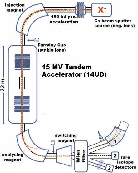
The Journal of Science Extension Research – Vol. 1, 2022 education.nsw.edu.au 67
Data Collection
Each test took approximately 65 minutes corresponding to 120 loops. Here, a loop is defined measuring the 92ZrF5- current for 10 seconds, switch the magnet to 94ZrF5- andmeasure this current for 10 seconds and then switch back to 92ZrF5(total of 32.8 seconds). The inclusion of two stable isotopes gives an additional metric, the ratio between the two isotopes aids in indicating sample stability. Due to the sample
physically changing when being sputtered, readjustments of beam
focusing is neededoccasionally. ‘Tuning loops’ where this adjustment was performed were excluded. Sample 6 was stopped after 91 loops, because the output was insignificant.
The raw data was retrieved from the system and included into an excel document foranalysis.
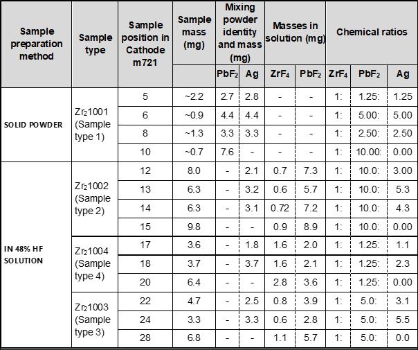
The Journal of Science Extension Research – Vol. 1, 2022
Table 1. Sample Preparation Method and Type Chemical Composition of Each Sample. Details of the samples including their types, the sample preparation method used, the relevant sample masses and the powder mass, as well as the chemical ratios adjusted to ZrF4.
education.nsw.edu.au 68
Data Analysis
The accelerator’s outputted data was the collected ion current for both isotopes, as well as the isotopic ratio for each loop. From there, the total charge and hence total number of particles were calculated in accordance with the quantification of time generated from the initial ten tuning loops.
To compare between samples and sample types, three factors are used to describe the sample output and stability:
The total number of particles, which is the current integrated over time. A highertotal number of particles for the radioisotope tests reduces the margins of errorand increases the sensitivity.
The time that the sample outputs a constant current from the beginning of the test reflects stability of the ion source. Low values indicate the current droppedor was too unstable.
Finally, the average standard deviation of the mean of the isotopic ratioindicates how the ratios between isotopes varied within the test, which also indicates stability at the ion source.
Performing a statistical test was inappropriate for the data collected, as the continuousvariable tests assume the dependent variable fits a normal distribution, which this datadoes not. Also, the number of repetitions of samples was low, as no two samples wereidentical, and no statistical test is valid to run based on the small population size. This
investigation is hence regarded as a trial, from which a general indication of trends isto be derived.
Risk assessment
The possible risks of using the AMS setup were discussed. The tandem accelerator was not used in the test, hence the only threat to health was x-ray emissions from theion source, though while the ion source was in operation, all participants were safe in the control room, which is a great distance away from the ion source. Also, evacuation procedures wherein all involved participants are evacuated to an outdoor meeting point were prepared for.
Ethics Statement
This research was conducted under the direct supervision of Postdoctoral Fellow Dr Stefan Pavetich and PhD Student Dominik Koll from the Australian National University(ANU). It was conducted at the Heavy Ion Accelerator Facility (HIAF) at the ANU, andhence was enacted in accordance with their governmentally mandated safety regulations. Permission from the ANU staff was granted before the data was given foranalysis.
Results
The samples prepared as powder (type 1) generally have lower stable times, lower total output, and greater overall isotopic ratio variance. The samples prepared in solution demonstrated higher stable times, higher mean total particles, and smaller isotopic ratio variance. The summary statistics are displayed in Table 2.
The Journal of Science Extension Research – Vol. 1, 2022
education.nsw.edu.au 69
Table 2. Results Summary of Data. Includes the three indicators of sample efficacy, along with the mean isotopic ratio and detector current details, which support quantification of the stability of both outcomes, as well as the strength of maintained current. Both the total particles and detector current is an average of the two isotopes, to illustrate the general current tendencies.
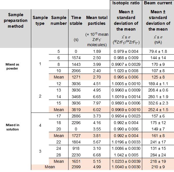
The aqueous samples, specifically type 2 and individual sample 15, displayed the most constant current and isotopic ratio, outputted the highest total amount of
particles, and remained stable for the entire time. Therefore, the total number of molecules plot is virtually linear, and the current fluctuates minimally in Figure 2.
The Journal of Science Extension Research – Vol. 1, 2022
education.nsw.edu.au 70
The solid samples, specifically type 1, and individual sample 6, displayed the least constant current and isotopic ratio, outputted the second least total amount of particles, and remained stable for the 5th least amount of time. The sample was
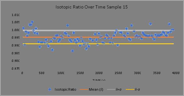
stopped after 91 loops, as previously discussed. The total number of molecules only grows insignificantly after the first approximately 1800 seconds, given the negligible beam current. The current fluctuates greatly (Figure 3 & 4)
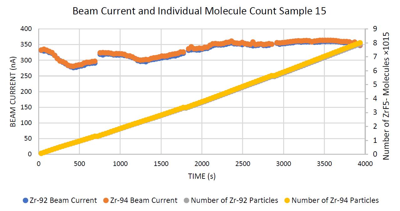 Figure 2. Sample 15, demonstrating an example of a stable sample with a stable current output, in terms of current and molecular count. This sample was the most stable and outputted the highest number of particles. The interruptions in the current curves are the loops where the beam focusing was retuned.
The Journal of Science Extension Research – Vol. 1, 2022 education.nsw.edu.au 71
Figure 3. Sample 15, demonstrating an example of a stable sample with a stable current output, in terms of isotopic ratio variance. This sample was the most stable and demonstrated the lowest ratio variance.
Figure 4. Sample 6, demonstrating an example of an unstable sample, in terms of current and molecular count. This sample was the least stable and outputted the lowest number of particles
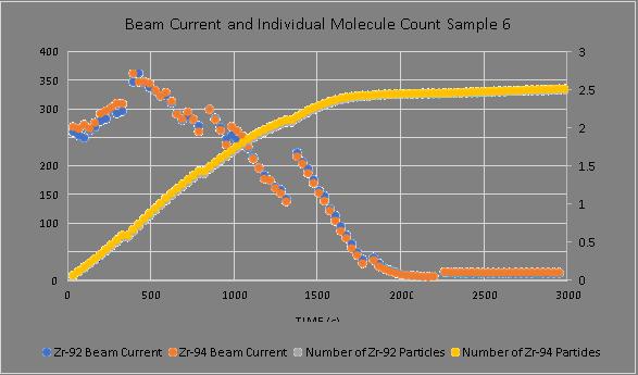
Figure 6 shows sample type 2 remained the most constant of the three sample types, beginning with a similar current to types 1 and 4, though sustaining the
current for the entire 120 loops. Sample type 3 began with a large output of current, though quickly decreased in magnitude. Sample type 1 decreased the most expeditiously.
Figure 6. Contrasting the sample types' mean ability to maintain a constant current, taking the mean of all constituent samples of a sample type, and removing all tuning loops. Shows the relative inconsistencies of sample 1, 4, and 3 to sample 2
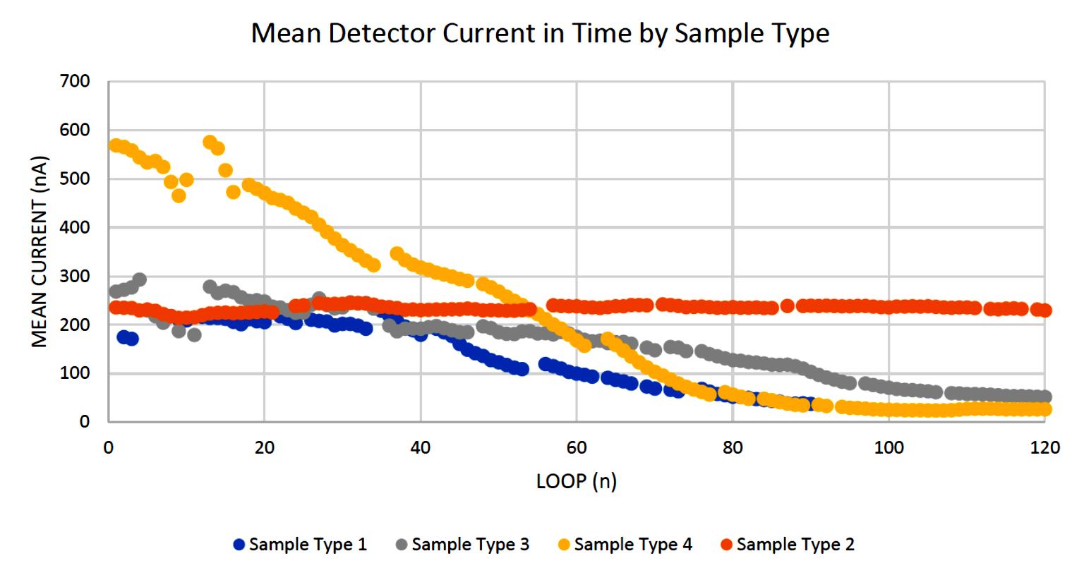
The Journal of Science Extension Research – Vol. 1, 2022 education.nsw.edu.au 72
Figure 7 shows the 92Zr/94Zr ratio for sample type 1 varied the most throughout the loops. The ratio for sample type 2 remained the most constant and was
closest to 1. For sample types 3 and 4 there was a similar large variance, and sample type 4 demonstrated an isotopic ratio furthest from 1.
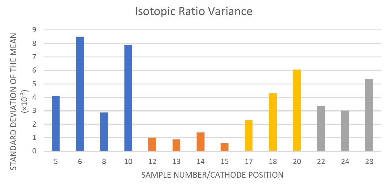
Figure 7. Contrasting the sample types' mean ability to maintain a constant isotopic ratio, taking the mean of all constituent samples of a sample type, and removing all tuning loops. This process introduced many inconsistencies in the smoothness of the data, as illustrated with large variance of data points.
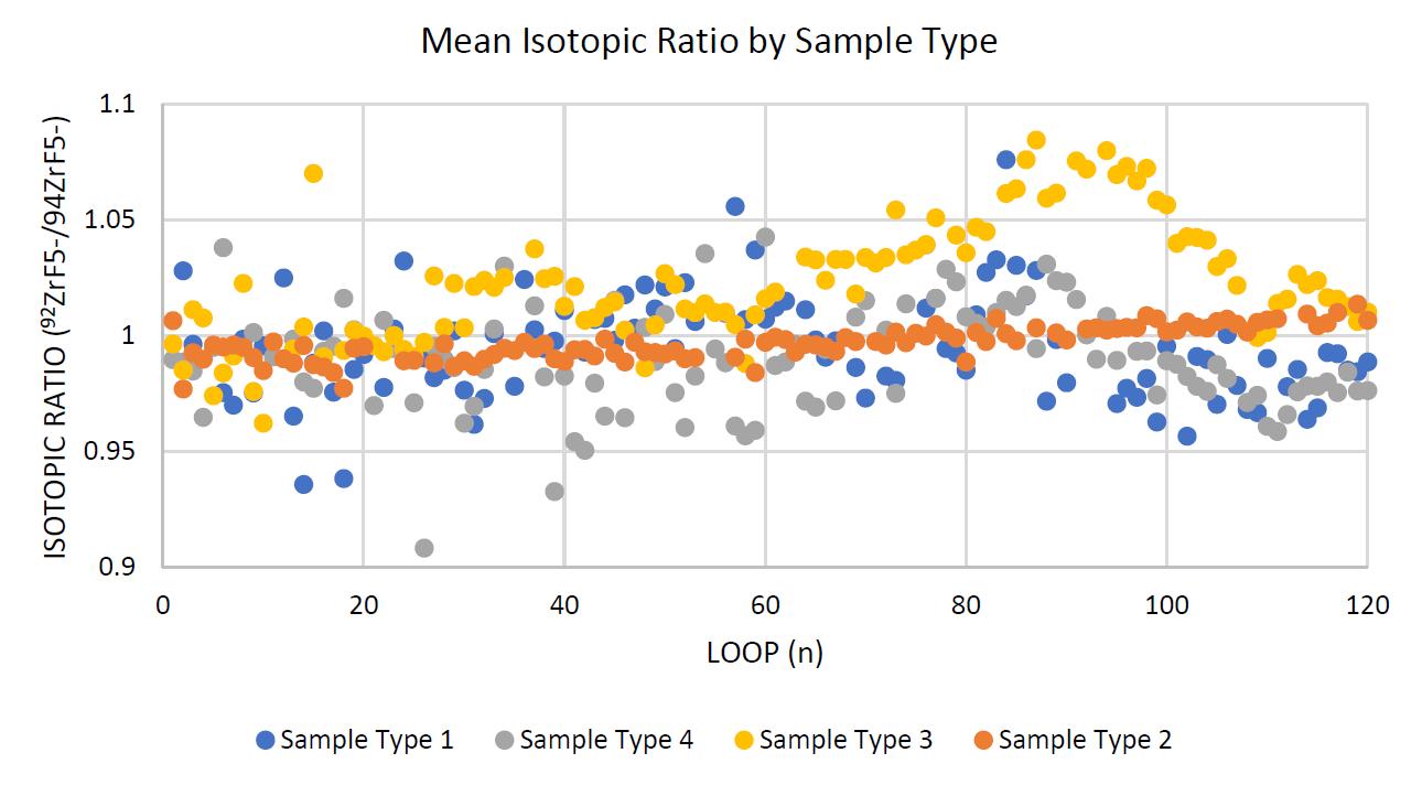
The standard deviation of the mean of each sample ratio is represented in Figure 8. This shows that sample type 1
varied greatly, and sample type 2 consistently varied the least
The Journal of Science Extension Research – Vol. 1, 2022 education.nsw.edu.au 73
The time each sample outputted a stable current for is shown in Figure 9. Sample 1 and 3 each had a sample that was never
stable, and sample type 2 clearly was consistently stable the entire time for almost all samples
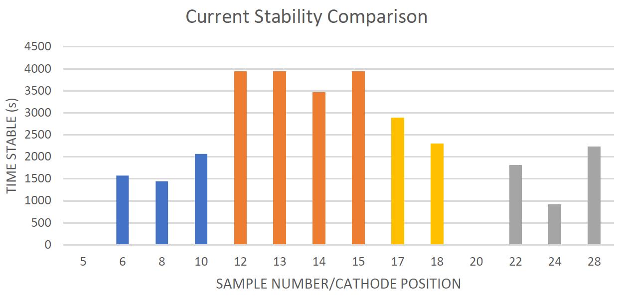 Figure 8. Showing the variances of the isotopic ratio per sample, colour coded for sample types. The bars are colour coded in accordance with their sample type in the same colours as the previous figures.
The Journal of Science Extension Research – Vol. 1, 2022 education.nsw.edu.au 74
Figure 9. The time each sample remained stable from the start of testing to the first sharp drop. The bars are colour coded in accordance with their sample type in the same colours as the previous figures
Discussion
The aim of this project was to investigate different compounds for high yield AMS 93Zrby studying temporal behaviour of ion currents of stable 92Zr and 94Zr, and to draw conclusions on the general trends of sample composition ratios used in sample synthesis.
As explained in the data analysis section, for a sample to be considered efficacious itmust maintain for the longest time possible a stable and large current and a stable isotopic ratio, as these factors are indicative of sample types which will create the highest possible sensitivity, precision, and accuracy for AMS of 93Zr.
As predicted, the sample types mixed in solution with hydrofluoric acid demonstrateda more desirable, stable, and higher output over a longer procession of loops than those mixed as solid powders. The samples mixed as powder in sample type 1 demonstrated lower and lesser desirable results. This is likely because as the constituent chemicals were combined as solids, the ionic lattices were not dissociatedand hence a less integrated synthesis of molecules within the samples was achieved.
This is reflected in the current output fluctuations (Figure 8) as the sputtering encountered different layers of chemicals with higher or lower abundances of constituent chemicals. The chemicals combined in solution dissociated, which alloweda greater miscibility within solution and hence greater homogeneity of chemical constituents within the samples.
Of the sample types mixed in solution; sample type 2 clearly demonstrated the
highest mean total particles (Table 2) by sustaining a moderate current for the entirety of the loops tested (Figure 7) with exceedingly high time stable values (Figure 9), and an especially stable mean current (Figure 6). In addition, the isotopic ratio of the sample type was very consistent (Figures 3 and 7) with the variance being the lowest of all samples (Table 2). These results are the most ideal of the sample types, and the mean isotopic ratio ZrF4:PbF2 was approximately 1:10.
Sample type 3 started with an exceptionally large current and quickly decreased (Figure 6). This meant while the mean total particle count was high for the sample type (Table 2), it had large variances. The instability was also evident in the isotopic ratio metrics, wherein the mean variance was close to sample type 4, which performed markedly worse. The sample type was composed of samples with a mean isotopic ratio ZrF4:PbF2 approximately 1:5.
Of the aqueous samples, sample type 4 demonstrated the lowest mean total particles (Table 2) by the current quickly falling and not returning for the entirety of the loops tested (Figure 7) with exceptionally low time stable values (Figure 9), and an especially instable mean current (Figure 6). In addition, the isotopic ratio of the sample type was very inconsistent (Figures 3 and 7) with the variance being the highest of all aqueous samples (Table 2). These results are the least ideal of the sample types, and the mean isotopic ratio ZrF4:PbF2 was approximately 1:1.25.
The significance of sample 15 outperforming the other samples in sample type 2 with remarkably similar
The Journal of Science Extension Research – Vol. 1, 2022 education.nsw.edu.au 75
chemical ratios is likely due to uncontrolled variables, such as the total amount of sample material, the geometry of the cathode, and sputtering crater inconsistencies. Therefore, variations are expected. The investigation remains valid, as the tests were conducted in a controlled environment with all random errors possibly eliminated and a strict methodology was followed, in accordance with the safety and scientific efficacy policies of ANU.
There was no significant correlation found between any of the variables detailed in the results table to the ratio of silver powder to ZrF5- molecules, nor the masses of silver powder themselves. However more testing outside the scope of this study must be undertaken to determine the extent of correlation more conclusively.
There is a clear positive correlation between the parts of PbF2 to every part ZrF4 in the sample and the ratio’s success in being stable and having a high current output. The relationship is causal, as the controlled environment of the 14UD eliminated all other variables. It is also clear the mixing method and chemical ratios of Sample 2 was the most indicative of sample success.
This project applies to the future of AMS by aiding to improve analysis of the radioisotope 93Zr, the ANU AMS team is currently working on. They can use the conclusions drawn in this paper to help inform the next step they take in achieving the ‘required sensitivities’ of the 14UD’s AMS of 93Zr capabilities for ‘applications in nuclear astrophysics’ and nuclear waste management (Pavetich et al., 2019).
Conclusion
The present study aimed to determine which of the four sample types prepared for AMS of 93Zr would perform most effectively, by maintaining a stable current for the longest time possible, sputtering the maximum number of individual molecules of ZrF5- and showing the least variance in the isotope ratio and current output. It was found that sample type 2 clearly performed most desirably, which was mixed in solution and had a mean ratio of approximately 1:10 of ZrF4 to PbF2. Generally, the samples mixed in solution performed better, and increasing the amount of PbF2 relative to ZrF4 gave a higher and more consistent anion beam output. Therefore, there is a positive correlation between the parts of PbF2 to every part ZrF4 in the sample and the ratio’s success in outputting a high and stable anion beam.
References
Accelerator mass spectrometry. (2021). Retrieved from ANSTO: https://www.ansto.gov.au/acceleratormass-spectrometry
Baglin, M. C. (2011). Nuclear Data Sheets for A = 93. Nuclear Data Sheets, 112, 1163-1389. doi:https://doi.org/10.1016/j.nds.2011.04. 001
Carey, A. (2015). Refining Methods for Ultra-Sensitive Detection of Zirtconium93.Honours Thesis, The Australian National University.
Fifield, L. K., Tims, S. G., Stone, J. O., Argento, D. C., & De Cesare, M. (2010). Ultra-sensitive measurements of 36Cl
The Journal of Science Extension Research – Vol. 1, 2022 education.nsw.edu.au 76
and 236U at the Australian National University. Nuclear Instruments and Methods in Physics Research B, 268, 858-862. Retrieved from https://doi.org/10.1016/j.nimb.2012.04.02
Kutschera, W. (2016). Accelerator mass spectrometry: state of the art and perspectives. Advances in Physics, 1(4). Retrieved from https://www.tandfonline.com/doi/full/10.10 80/23746149.2016.1224603
Leckenby, G. (2017). Remodelling a multi-anode ionisation chamber detector for accelerator mass spectrometry of 53Mn. Canberra: Honours Thesis, The Australian National University. Retrieved from
https://doi.org/10.25911/5d69077cdccd8
Lu, W., Anderson, T., Bowers, M., Bauder, W., Collon, P., Kutschera, W., . . . Steier, P. (2015). Zr/Nb isobar separation experiment for future 93Zr AMS measurement. Nuclear Instruments and Methods in Physics Research B, 361, 491-495. Retrieved from https://doi.org/10.1016/j.nimb.2015.01.07
Marks, A. (2021). Physics of Uranium and Nuclear Energy. (ANSTO, Editor) Retrieved from World Nuclear Association
website: https://worldnuclear.org/information-library/nuclearfuel-cycle/introduction/physics-of-nuclearenergy.aspx
Pavetich, S., Carey, A., Fifield, L., Froehlich, M. B., Halfon, S., Kinast, A., . . . Weissman, L. (2019). 93Zr developments at the Heavy Ion Accelerator Facility at ANU. Nuclear Inst. and Methods in Physics Research B, 438, 77-83. Retrieved from https://openresearchrepository.anu.edu.au/handle/1885/20321 8
Wallner, A., Feige, J., Fifeild, L. K., Froehlich, M. B., Golser, R., Hotchkins, M.A., . . . Tims, S. G. (2020, August 24). 60Fe deposition during the late Pleistocene and the Holocene echoes past supernova activity. Proceedings of the National Academy of Sciences of the United States of America, 36(117), 21873-21879. Retrieved from
https://doi.org/10.1073/pnas.1916769117
Winter, M. (2021). Zirconium: isotope data. (U. The University of Sheffield and WebElements Ltd, Editor) Retrieved from WebElements:
https://www.webelements.com/zirconium/i sotopes.htm
8
1
The Journal of Science Extension Research – Vol. 1, 2022 education.nsw.edu.au 77
The Potential Use of Scarab Beetle Larvae in Composting
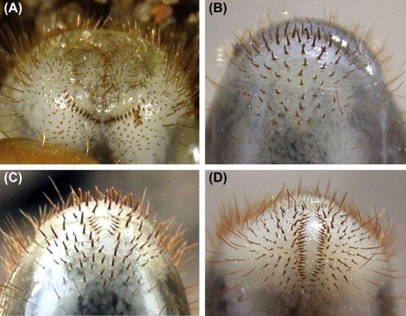 Liam Foley
Killarney Heights High School
Liam Foley
Killarney Heights High School
The aim of this paper is to determine whether scarab beetle larvae can be used to help in the process of composting. The experiment was conducted over the course of seven weeks in which varying amounts of Xylotrupes australicus larvae were placed into containers containing either composted or uncomposted substrate. It was found that there was no statistical difference between the growth rate of the larvae in composted and uncomposted substrate. An increase in growth was observed in all larvae regardless of which substrate they were in. Visually, the substrate in the containers that had held larvae appeared to be broken down much finer and contained fecal pellets when compared to the containers that had not held any larvae.
Literature review
The Scarabaeidae family, commonly known as the scarab beetle family is a diverse family consisting of approximately 30,000 species of beetle of which there are over 2,000 species described in Australia (CSIRO). The larvae of scarab beetles have three stages which are known as instars (DPI), and the larvae are usually very difficult to distinguish. Species identification often relies on differences in the pattern of the hairs, called setae, present on the underside of the terminal abdominal segment, called the raster (Timothy Gibb, 2015).
Examples of setae patterns can be seen in figure 1.
The immature stages of many species feed solely on decaying organic matter and animal faeces. However, other species feed on decaying organic matter and living plants; generally roots and/or basal stem tissue (GreenLifeIndustry, 2017). Such species are pests that can cause serious damage. In natural ecosystems, beetles and their associated microorganisms perform important functions as prime contributors to the degradation of organic matter (K. RojasJiménez, M. Hernández. 2015). Due to
Figure 1. Rastral setae patterns of four common agricultural pests (Timothy Gibb, 2015)
The Journal of Science Extension Research – Vol. 1, 2022 education.nsw.edu.au 78
the difficulty in distinguishing the larvae of pest species from other species, this often leads to the indiscriminate killing of native species. This is further exacerbated in the gardening community where misinformation often leads to the recommendation that any beetle larvae should be eradicated. I have frequently observed this advice being given in the Facebook group, “Gardening Australia”, as well as several other gardening related groups. Through conducting my experiment I want to explore a potential alternative to indiscriminately killing scarab beetle larvae. There are several species of scarab pest species in Australia, one of the most well known ones being Heteronychus arator, commonly known as the African black beetle. H. arator is a common agricultural pest, Larvae prune or completely sever roots of perennial grasses and in severe cases where larval populations are high, pasture becomes patchy and can be rolled back like a carpet. (Cesar, 2015). Several studies have been conducted on these agricultural pests in order to gain a better understanding of their feeding habits and preferences. In a 1977 study titled, “Effect of plant species and organic matter on feeding behaviour and weight gain of larval black beetle, Heteronychus arator (Coleoptera: Scarabaeidae)” conducted by P. D. King looked at the effect of several plant species on the movement and feeding behaviour of H. arator and the influence of organic matter on those responses. The results of the experiment were determined using choice chamber testing over a 21 day trial period, repeating the test until fifty larvae had been tested. They monitored weight gain, movement and the number of fecal pellets produced by each larva. In his results he highlighted that organic matter
stimulated feeding and increased weight gain (P.D. King, 1977).
Household compost includes several organisms bringing about the whole process of composting. It has its own micro flora-fauna and macro flora-fauna which include scavengers, predators and decomposers. Although the role of other organisms is noticed, there is a lot of emphasis on either microorganisms or earthworms, not much attention is given to other macro organisms often present in compost (Gayatri. A et Al, 2009).
Scientific Research Question
Will Xylotrupes australicus larvae grow more in composted material or uncomposted material?
Scientific Hypothesis
The larvae will grow more as a result of feeding on the composted substrate.
Materials and Methodology
Two types of substrate were used in the experiment. The first substrate was homemade compost from a garden compost bin as shown in Figure 2.

The Journal of Science Extension Research – Vol. 1, 2022 education.nsw.edu.au 79
Figure 2: Homemade compost
The second substrate was a mixture of finely chopped uncomposted organic matter. The carbon rich components of this substrate were dried leaves, sugar cane mulch, cocopeat and were mixed in a ratio 2:3:1, and the nitrogen rich components were a random mixture of finely diced household vegetable scraps (such as leafy greens, potato peels, and carrot tops). The carbon-rich and nitrogen-rich components were mixed in a ratio of 25:1 as recommended by the Plant Natural Research Centre website, as shown in Figure 3. 1 part store bought compost was also added to the mixture in order to aid in the composting process by adding the appropriate microorganisms.
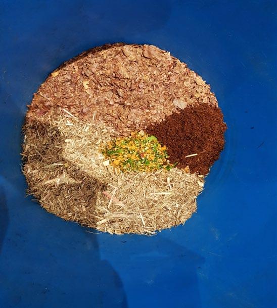
The experiment was conducted using 8 300ml plastic containers with ventilation holes added to the lids. Half of the containers were filled with the compost, while the other half were filled with the uncomposted mixture. 75ml of water was added to each of the containers containing the uncomposted substrate. Varying numbers of small Xylotrupes australicus larvae were weighed and then added to the containers, as shown in Figure 4 below, which were labeled with a reference indicating composted or uncomposted and the number of larvae.
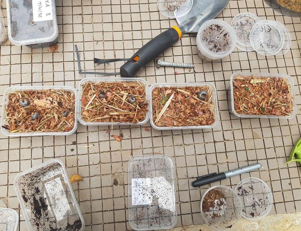
These combinations are represented in Table 1 below.
0 Larvae C0 U0
1 Larva C1 U1
2 Larvae C2 U2
3 Larvae C3 U3
All containers were placed in a cupboard to remain undisturbed for the duration of the experiment with the exception of weekly weigh-ins.
On a weekly basis the containers were removed from the cupboard and the larvae in each container were weighed individually using a I-2000 digital platform scale provided by KHHS, with a stated accuracy of ±0.01g.
Results
All measurements were taken in grams and recorded to two decimal places, presented in Table 2 below. Note the reference to “random” is to highlight the fact that the weights recorded in a column
Figure 3: Uncomposted substrate prior to being mixed
Composted Uncomposted
Figure 4: Containers with varying numbers of larvae
Table 1: Container Labeling
The Journal of Science Extension Research – Vol. 1, 2022 education.nsw.edu.au 80
are not necessarily for the same larva cells in the table. The deceased larvae with each sample. Additionally some were not included in the calculations for larvae died and this is indicated by grey averages.
An analysis was generated on the raw data, to calculate the average weight of the larvae in each container, this is shown in Table 3
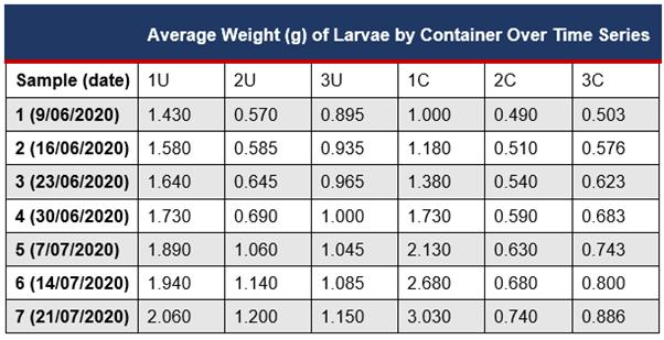
Table 3: The average weight of larvae by container over time
This data was then used to calculate the average weight of all the larvae each week, based on substrate type as shown in Table 4. This data is represented in Figure 5.
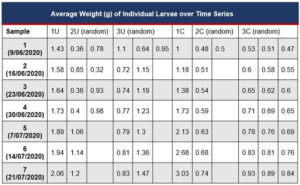 Table 2: Raw data.
education.nsw.edu.au 81
A T-test was conducted to see if the difference between the two means of weight of the larvae in uncomposted and composted substrate was significant at ����<0.05, refer to Table 5.
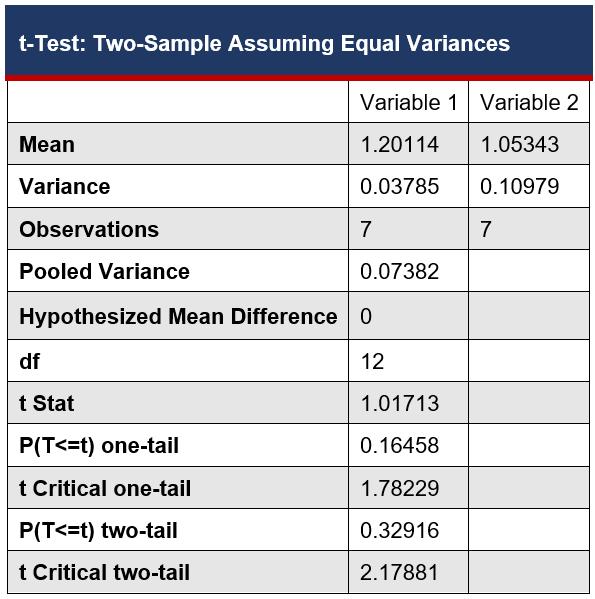
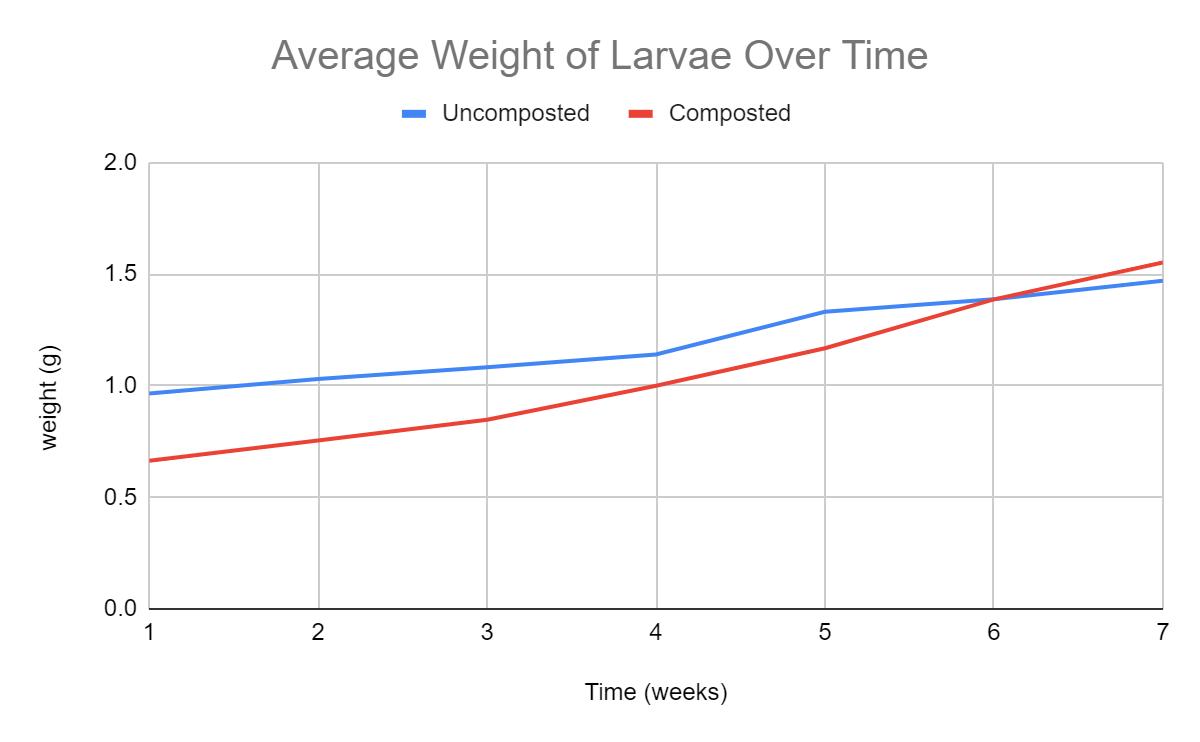
Average Weight (g) of Larvae by Substrate Over Time Series 1 2 3 4 5 6 7 Uncomposted 0.965 1.030 1.083 1.140 1.332 1.388 1.470 Composted 0.664 0.755 0.848 1.000 1.168 1.387 1.552
Table 4: The average weight of larvae by substrate over time
Figure 5: Average weight of larvae over time
education.nsw.edu.au 82
Table 5: T- Test
Discussion
While all larvae gained weight, and the graph in Figure 5 appears to indicate an increased growth rate for the larvae in the compost substrate, by doing a t-test I determined that I could not reject the null as my p-value was greater than 0.05. This meant that there was no statistical difference between the growth rate of larvae in the composted and uncomposted substrate. My null hypothesis was that the larvae will not grow more as a result of feeding on the composted substrate. Upon visual comparison of the containers containing larvae with those that did not house any larvae (U0 and C0), the matter appeared to be broken down much finer and contained fecal pellets. Although there is no statistical difference between the growth rates, it is clear that there is a general increase in the weight of the larvae in both substrates over time. There was a 52% increase in the average weight of larvae in uncomposted versus a 134% increase for larvae in the composted substrate. This indicates that there is potential for scarab beetle larvae as composting organisms as they grew even when feeding and therefore, by implication, helped break down material in substrates at two drastically different stages of decomposition. There were a number of factors that affected the results of my experiment, the main one being temperature. As X. australicus is a tropical/subtropical species mainly found in NE NSW and QLD, they are not suited to Sydney's temperate climate, especially in winter which is where and when the experiment was conducted. As they received no artificial warmth, their metabolism would have been much
slower and therefore they would have consumed less and as a result grown less than if the experiment had been conducted in summer when the temperatures are warmer. The cold temperatures may have also been the cause of death of the three larvae that died during the experiment. This is likely because first instar larvae are much less tolerant of cold temperatures. The limitations of my experiment also included the limited range of species, the size of the containers, and the quality of the substrate. If I were to repeat the experiment I would use a local species of scarab beetle and I would conduct the experiment in summer when it is warm, I would also use third instar larvae as they are more hardy than first instar larvae, they consume more food than previous stages and gain more weight (GreenLifeIndustry, 2014). Further experiments could be conducted to test the fertility of compost broken down by scarab beetle larvae versus that that hasn't. This could be done by measuring the growth of plants grown in compost which has been broken down by scarab beetle larvae versus compost which has not been broken down by scarab beetle larvae. Future research should be done on the diets and feeding habits of native scarab species in order to determine which species may act well as potential composters.
Conclusion
After conducting a t-Test it was determined that there was no statistical difference between the growth rate of larvae in the composted and uncomposted substrate, this is because the p-value was over 0.05. It was demonstrated that X. australicus larvae
The Journal of Science Extension Research – Vol. 1, 2022 education.nsw.edu.au 83
will consume and grow in either substrate. A visual comparison of the containers containing larvae with those that did not house any larvae (U0 and C0), revealed that the matter appeared to be broken down much finer and contained fecal pellets. I determined that there is potential for scarab beetle larvae to be used as composting organisms as
Reference List Britannica. (2011). Scarab Beetle.
Retrieved June 26 from https://www.britannica.com/animal/scarab -beetle
Cesar. (2017). African Black Beetle. Retrieved June 26 from http://cesaraustralia.com/sustainableagriculture/pestnotes/insect/african-blackbeetle
CSIRO.(2020). SCARABAEIDAE Scarab
Beetles or Cockchafers or Dung Beetles. Retrieved June 26, 2020, from https://www.ento.csiro.au/education/insec ts/coleoptera_families/scarabaeidae.html
Gibb, T. (2015). Contemporary Insect Diagnostics, Retrieved June 26, 2020, from https://www.sciencedirect.com/topics/agri cultural-and-biologicalsciences/scarabaeidae
Goodyer, G. Nicholas, A. Scarab grubs in northern tableland pastures. Retrieved June 26 from
https://www.dpi.nsw.gov.au/__data/asset s/pdf_file/0008/110213/scarab-grubs-innorthern-tableland-pastures.pdf
GreenLifeIndustry.(2014). Managing
Scarab Beetles in Production Nurseries. Retrieved June 26 from
they grew even when feeding and therefore, by implication, helped break down material in substrates at two drastically different stages of decomposition. If the experiment is to be repeated, there are several factors that should be taken into consideration such as species and temperature in order to produce more accurate results.
https://www.greenlifeindustry.com.au/Atta chment?Action=Download&Attachment_i d=2068
Hernández, M. Rojas-Jiménez, K. Isolation of Fungi and Bacteria
Associated with the Guts of Tropical Wood-Feeding Coleoptera and Determination of Their Lignocellulolytic Activities. Retrieved June 26 from https://www.hindawi.com/journals/ijmicro/ 2015/285018/
P.D. King (1977) Effect of plant species and organic matter on feeding behaviour and weight gain of larval black beetle, Heteronychus arator (Coleoptera: Sacrabaeidae). Retrieved June 6 from https://www.tandfonline.com/doi/abs/10.1 080/03014223.1977.9517968
PlanetNatural. (2020). Carbon-toNitrogen Ratio. Retrieved June 26, 2020, from
https://www.planetnatural.com/compostin g-101/making/c-n-ratio/
Sagade, G. Pejaver, K. (2009). Study of diversity of insect fauna from the household biocompost. Retrieved June 26, 2020, from
http://dspace.vpmthane.org:8080/jspui/bit stream/123456789/4648/1/MKP_32.pdf
The Journal of Science Extension Research – Vol. 1, 2022 education.nsw.edu.au 84
Microplastic Contamination of Urban and Bushland
Dominated Beaches of the Shoalhaven
Megan Jeffers
Ulladulla High School
Microplastics in the marine environment represent a form of pollution of increasing concern. This investigation examined two beaches in the Shoalhaven for microplastic abundance. A total of eight samples, four from Ulladulla Harbour and four from Termeil Beach, were collected and analysed using visual microscopy. Microplastic occurrence was detected in all samples, with Ulladulla harbour having an average of 66.75 plastic pieces per sample and Termeil Beach having and average 21.25 plastic pieces per sample. The results suggest that urban dominated beaches, as represented by Ulladulla Harbour, have a higher risk of microplastic occurrence. The most common items were fibres <630μm.
Key words: microplastic; urban; bushland; marine pollution.
Introduction
Marine anthropogenic litter is recognized as an emerging global pollutant. Plastic production is increasing each year, with 348 million tonnes being produced in 2017 worldwide (Garside, 2019). This plastic is dispersed by currents and winds, and persistent plastics rarely degrade, but instead become fragmented over time (Löder & Gerdts, 2015). Much of this plastic ends up in the oceans, with an estimated 5 trillion pieces weighing roughly 250 million tonnes in the global seas (Glaser, 2015). The distribution of microplastics in the ocean has effects, both direct and indirect, on marine fauna and local economies. The most abundant and problematic form of anthropogenic litter are buoyant and persistent plastics (Frias, et al., 2018). These most often occur in the form of microplastics, being defined as between 1μm and 5mm
(Masura, et al., 2015). They can be either primary (produced to be of microscopic size) or secondary (resulting from fragmentation) (Löder & Gerdts, 2015). Microplastics tend to present themselves as beach litter, floating litter, seafloor litter or biota litter (Joint Research Centre of the European Commission, 2013). The distribution of microplastics is largely dependent on density, and as most plastics have densities lower than seawater, they float on the water surface. However, some plastics can be suspended in the water column or sink into the sediment. Beaches, as intermediate environments, can accumulate floating, buoyant and sinking plastics (Löder & Gerdts, 2015).
Microplastics can have effects on marine life when ingested, by causing blockages throughout the digestive system (Löder & Gerdts, 2015). In addition, microplastics contain a mixture of chemicals added
The Journal of Science Extension Research – Vol. 1, 2022 education.nsw.edu.au 85
during manufacture and efficiently absorb Persistent, Bioaccumulative and Toxic contaminants (PBTs) from the environment. The ingestion of microplastics by aquatic organisms and the accumulation of PBTs have been central to the perceived hazard and risk of microplastics in the marine environment (Lusher, et al., 2017). This can also pose risks as toxic chemicals are propagated throughout the food web, with potential for entering human food sources.
While the risk of microplastics being consumed from fish by humans is minimal (as the gastrointestinal track is most often removed), microplastic pollution continues to increase thus, increasing the risk of microplastic ingestion and increasing the risk of negative effects from exposure to PBTs in humans (Cheung, et al., 2018). As there are no standardised methods for monitoring microplastic occurrence, there are significant gaps in knowledge, particularly with smaller sized microplastics (<150μm) (Löder & Gerdts, 2015). This research assesses microplastic contamination (occurrence and physical qualities) on urban and bushland dominated beaches in the Shoalhaven.
Literature review
Increased environmental awareness has led to a large amount of research into plastics in the environment. It is estimated that plastic pollution is composed of more than 5 trillion plastics pieces equal to roughly 250,000 tons in the global seas (Glaser, 2015). An increasing number of reports have been published concerning micro-plastic pollution in aquatic environments, however, these studies
continue to be updated and lack standardisation (Mai, et al., 2018). In an effort to standardise the methods for researching micro-plastic pollution, several papers have also been published reviewing common methods. These include methods for sampling, separation, identification and quantitation. Microplastics are commonly researched within water samples, sand samples, sediment and biota within the literature. For the purpose of this review, sand samples will be focussed upon. While the definition for microplastics is still under debate, the majority agree that microplastics are plastics from 1μm to 5mm (Löder & Gerdts, 2015) (Frias, et al., 2018) (Masura, et al., 2015).
Microplastics contain a mixture of chemicals, and also effectively absorb persistent, bio-accumulative toxic contaminants (PBTs) from the environment (Lusher, et al., 2017). Microplastic contamination within the environment will continue to increase as plastic production increases and ineffective methods are used for rubbish disposal. Currently, there are no standardised methods (Löder & Gerdts, 2015) and significant gaps in knowledge when it comes to smaller plastics and nanoplastics, and their possible effects on seafood safety (Lusher, et al., 2017).
Methods are broken up into three main sections, sampling, extraction and identification. The methods for sampling beach sediment is similar throughout the literature, however details differ between papers. Generally, sampling beach sediments requires non-plastics sampling and storage tools (Löder & Gerdts, 2015). However, the amount and nature of the samples differs. Sample amounts range from less than 500g to 10kg (Löder & Gerdts, 2015). Sampling tools include
The Journal of Science Extension Research – Vol. 1, 2022 education.nsw.edu.au 86
grab samplers, core samplers, dredge samplers, remotely operated vehicles (Frias, et al., 2018) and manual collection (spoon, trowel, shovel) (Löder & Gerdts, 2015). Generally the high tide line is sampled (Löder & Gerdts, 2015) (Sul, et al., 2017), from depths of 2cm (Sul, et al., 2017) to 30cm (Löder & Gerdts, 2015). The units of microplastic abundance depends on sampling approach, thus abundance is normalised to sampling area, sediment weight or volume (Löder & Gerdts, 2015).
Once sampled, extraction of the microplastics is then conducted. Once again, there is no standard protocol for the extraction of microplastics from samples, although two main methods are used, density separation (Löder & Gerdts, 2015) (Masura, et al., 2015) (Frias, et al., 2018) and dry sieving (Sul, et al., 2017). The density separation method uses sediment purification using hydrogen peroxide(H2O2) at 6-10% (Frias, et al., 2018) up to 30% (Löder & Gerdts, 2015) (Masura, et al., 2015). This can be carried out prior to separation (Frias, et al., 2018) or afterwards (Löder & Gerdts, 2015) (Masura, et al., 2015). Other ways to purify include rinsing with pure water or ultrasonic cleaning (Löder & Gerdts, 2015). However, purification should be carefully considered as brittle plastics can be degraded (Löder & Gerdts, 2015). Density separation includes adding a saturated salt solution of high density and agitating (by stirring, shaking, aeration etc.) for a certain amount of time, before allowing plastic particles to float to the surface or stay in suspension whilst the heavier sediments settle (Löder & Gerdts, 2015) (Masura, et al., 2015) (Frias, et al., 2018). The supernatant is then decanted and filtered to remove microplastics (Frias, et al., 2018) (Löder & Gerdts,
2015) (Masura, et al., 2015). The alternative method is dry sieving. Sand samples are dried and sieved through a series of sieves (Sul, et al., 2017) (Löder & Gerdts, 2015), and then sorted into size class before microplastics are identified (Sul, et al., 2017). Alternatively, plastics >500μm can be sorted manually under a microscope, with the smaller samples being purified and filtered (Löder & Gerdts, 2015).
Once extracted, the next step is identification of microplastics. This section is the most standardised section, with plastics being sorted into size and colour (Frias, et al., 2018) (Löder & Gerdts, 2015) (Masura, et al., 2015) as well as source, shape and degradation stage (Löder & Gerdts, 2015). As well as this, type (Frias, et al., 2018) (Löder & Gerdts, 2015) (Sul, et al., 2017) and chemical analysis can also be carried out (Frias, et al., 2018) (Löder & Gerdts, 2015). Once identified, results can be expressed as: no. Microplastics per area, no. Microplastics per volume, no. Microplastics per mass, mass of Microplastics per area or mass of Microplastics per volume (Frias, et al., 2018).
Most of the literature analysed are reviews of the various methods used by research papers. These have advantages as they mention a variety of methods, however, they do not review the results from these various methods. This means that there is a limited ability to compare results to other published papers. In addition, the majority of literature is based in Europe, including summaries of methods which are produced by European institutions. While the results from this research can give implications into microplastic pollution, further
The Journal of Science Extension Research – Vol. 1, 2022 education.nsw.edu.au 87
research is required to examine the extent of microplastic pollution in Australia.
Research question and hypothesis
The research question that will be investigated in this report is ‘Is there a higher rate of microplastic occurrence on urban dominated beaches than bushland dominated beaches in the Shoalhaven?’
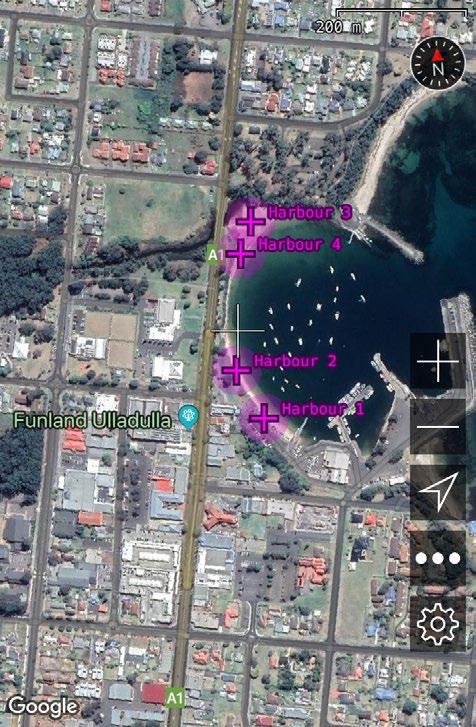
The Hypothesis states ‘Bushland dominated beaches will have a lower rate of microplastic occurrence than urban dominated beaches in the Shoalhaven’.
Therefore, the null hypothesis states that ‘There is no difference in microplastic occurrence between bushland dominated and urban dominated beaches in the Shoalhaven.’ The alternate hypothesis states ‘There is a difference in microplastic occurrence between urban dominated and bushland dominated beaches in the Shoalhaven.’
Method
Sampling
Sand was collected from two beaches in the Shoalhaven, the urban dominated beach being Ulladulla Harbour and the bushland dominated beach being Termeil beach.
in the middle (See figure 1) whilst practicing caution towards any hazards on the beach. The sand was sampled by excavating the top two centimeters of sand from 250cm2 quadrants. Non-plastic collection and storage tools were used to prevent plastic contamination.
A total of eight samples were collected, four samples from each beach, spaced in equal increments so that there was one sample collected from each end and two

Statistical Analysis
The collected data was analysed using Microsoft Excel. Because this data has a difference in variance, a one-tailed unpaired and un-equal variance t-test was used to demonstrate the difference in bushland and urban dominated beaches in the Shoalhaven in terms of number of microplastic pieces that occurred. Data collected was also demonstrated by number of plastic items per weight. In addition, descriptive statistics were also displayed in this study, including mean values alongside median values and standard deviation. A 0.05 level of significance was adopted.
Length Grain Size Dire ction Slope Ulladulla Harbour 1500m Fine East 6° Termeil Beach 600m Medium -fine East 7°
Figure 1: Sample sites from Ulladulla
The Journal of Science Extension Research – Vol. 1, 2022 education.nsw.edu.au 88
Results
Abundance of particles
The physical characteristics of each beach sampled are shown in tables. In this study, the presence of microplastics on beaches in the Shoalhaven was confirmed. A total of 352 microplastic pieces were identified with 75.85% being from Ulladulla Harbour Beach and 24.15% being from Termeil beach. Each of the four samples from both beaches were contaminated. The recorded results were adjusted using the number of microplastics that occurred on blank petri dishes that were analysed parallel to each sand sample.
dominated beach than the bushland dominated beach (p=0.0039, a=0.05). On average, 66.75 microplastic pieces were found in each 500g sample from Ulladulla Harbour, while only an average of 21.25 was found in each 500g sample from Termeil beach.
Types, colours and sizes of plastics
Key: U=Ulladulla; T= Termeil
a.) >850; b.) 850-630; c.) 630-315; d.) 315180; e.) 180-75; f.) <75
The mean number of microplastic items was significantly higher in the urban
A total of 204 fibres were observed in Ulladulla samples, which accounted for 76.4% of the plastics from Ulladulla Harbour. A further 56 fragments were found making up 20.97%, and 7 beads which constituted the last 2.62% of plastics from Ulladulla Harbour. Fibres were also the most common microplastic from Termeil beach, which constituted 62 fibres which made up 72.94% of the plastic pieces found at Termeil, followed by 23 fragments which made up the last 27.06%. Overall, fibres were the most common microplastic (75.57%), followed by fragments (22.44%) and beads (1.44%). Ten different colours of plastics were observed, with the most common colour being clear, making up 35.51% of the total microplastic pieces. Other plastic items were black, pink, blue, purple, white, orange, green, brown and yellow. There was a higher variety of colours on Ulladulla Harbour beach than Termeil Beach, in which only seven colours were observed.
U 1 U 2 U 3 U4 T 1 T 2 T 3 T 4 a.) 5 1 - 7 - 0 0 0 B.) 16 1 9 18 0 0 1 0 c.) 12 11 26 34 5 4 14 2 d.) 15 3 14 16 9 2 6 6 e.) 8 8 8 13 3 2 3 2 f.) 15 7 6 14 15 4 3 4 Tota l 71 31 63 10 2 32 12 27 14
The Journal of Science Extension Research – Vol. 1, 2022 education.nsw.edu.au 89
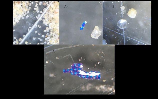
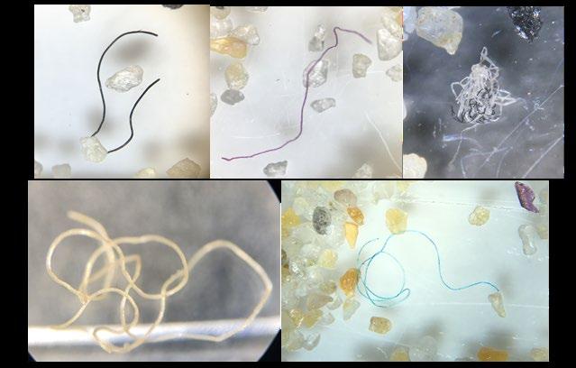 Figure 2: a) Examples of fragments b) Example of bead
The Journal of Science Extension Research – Vol. 1, 2022 education.nsw.edu.au 90
Figure 3: Examples of fibres
Occurrence of Microplastics

90 0 10 20 30 40 50 60 70 80 Number of Plastic Pieces >850 850-630 630-315 315-180 180-75 <75 Size(μm) Ulladulla Termeil Identification Category Variable Ulladulla Harbour 267 Termeil Beach85 Types of Plastic Fibre Fragment Bead 204(76%) 56(21%) 7(3%) 62(73%) 23(27%) 0 Colours of Plastic Green Blue Black White Clear Pink Purple Orange Brown Yellow 6(2%) 43(16%) 61(23%) 18(7%) 97(36%) 34(13%) 3(1%) 1(0.5%) 3(1%) 1(0.5%) 1(1%) 25(29%) 20(24%) 4(5%) 28(33%) 5(6%) 2(2%) 0 0 0 Size of Plastic >850 850-630 630-315 315-180 180-75 <75 13(5%) 44(16%) 83(31%) 48(18%) 37(14%) 42(16%) 0 1(1%) 25(29%) 23(27%) 10(12%) 26(31%) The Journal of Science Extension Research – Vol. 1, 2022 education.nsw.edu.au 91
The mean number of microplastic items was significantly higher in the urban dominated beach than the bushland dominated beach (p=0.0039, a=0.05). On average, 66.75 microplastic pieces were found in each 500g sample from Ulladulla Harbour, while only an average of 21.25 was found in each 500g sample from Termeil beach.
Discussion
This study aimed to determine whether or not there is a significant difference in the abundance of microplastics on urban dominated or bushland dominated beaches in the Shoalhaven. Visual identification was used to determine the rate of occurrence of microplastics in four 500g samples from two beaches, Ulladulla Harbour representing an urban dominated beach and Termeil Beach representing a bushland dominated beach. Ulladulla Harbour was chosen as the urban dominated beach in this study as it is situated in the most populated local area, as well as being influenced by industrial fishing and having Millards creek empty into the harbour, acting as storm water runoff. Termeil Beach was chosen to represent the bushland dominated beach as it is surrounded by bushland, having the nearest settlement 3km away. In addition, it is only accessible by 4wd, meaning it experiences a low level of human interaction.
In this study, it was found that the mean number of plastic particles was significantly higher in Ulladulla harbour (urban) than Termeil Beach (bushland). On average, 66.75 microplastic pieces were found in each 500g sample from
Ulladulla Harbour, while only an average of 21.25 was found in each 500g sample from Termeil beach.
The higher abundance of microplastics on Ulladulla Harbour beach may be related to the difference in environment, and the different uses of the areas. Microplastics can be introduced into the environment through land-based sources including sewage discharge, illegal dumping, storm-water runoff, industrial activities and accidental spillage during transportation (Cheung, et al., 2018)
In this study, fibres were found to be the most common type of microplastic for both sample sites. Fibres were also the most common microplastic in previous studies of microplastics in the marine environment (Cheung, et al., 2018). Other studies did not find any fibres (Sul, et al., 2017). However, this study only analysed samples >1mm, meaning that fibres may have been present in smaller size categories.
In this study, the two beaches that were examined had fine sand, with Ulladulla Harbour also having some medium grain sand, as well as some pebbles. The microplastics observed were most predominant in size categories that had the largest mass of the sand sample. Due to this, data cannot be accurately compared to studies such as conducted by (Sul et al). that only examine samples of in larger size categories. In the above mentioned study, the majority of beaches examined had fine grain size, meaning that analysing only categories of >1mm reduces the accuracy of their results as it is likely that the majority of microplastics reside in the smaller size categories that match the grain size of the beaches.
The Journal of Science Extension Research – Vol. 1, 2022 education.nsw.edu.au 92
Currently, the reliability and comparability of the literature surrounding microplastics in the marine environment is hampered by the huge variety of methodologies applied. Thus, one basic aim must be the standardization of methodologies for identification and quantification of microplastics in the marine environment, and the subsequent formulation of standard operating procedures (SOPs) (Löder & Gerdts, 2015). This should include the whole cycle of the assessment of microplastics in the marine environment, including sampling procedures, purification, and microplastic identification. Due to variety of methodologies used in the literature, there are complications when comparing data from this study with others.
In this study, the method of visual identification was employed. While this method has benefits, it also has limitations. If identifying by first using a density separation, some microplastics may not be counted depending of the density of the salt solution used. This can be impractical as salts of higher densities often have high costs and therefore are not economically efficient. The method of visual microscopy eliminates most costs, however, it relies heavily on the ability of the researcher to identify plastics. In this study, if there was any doubt about the nature of a particle, it was not counted as a plastic particle (Munno, n.d.). This means that the rate of microplastic occurrence may be lower than the actual abundance. However, while criteria for identifying plastic pieces was followed, without a chemical analysis, there is still the possibility that some particles identified as plastic pieces were misidentified, and were in actuality pieces of organic matter.
Another limitation with this method is that there is risk of contamination from airborne microplastic. To limit the risk of contamination, all materials used were not made of plastics. In addition, analysis was conducted in a low-dust room with minimal movements being made by the researcher to limit the movement of plastic fibres which may become airborne from clothing or other items in the room. Further actions taken to limit this risk include keeping samples covered for the maximum amount of time possible and running blanks parallel to the sand samples. These blanks were empty petri dishes that were treated the same as sand samples and analysed by visual microscopy. Blank petri dishes returned abundances of microplastics between 0 and 3, creating a degree of uncertainty.
In addition, 500g samples were analysed due to time restrictions. However, while the results from these samples give a reliable indication into the abundance of microplastics from their respective beaches, a larger sample size is required.
Recent research shows that the commonly applied method of visual inspection of samples alone is insufficient to identify microplastic particles in environmental samples, especially for particle sizes <500μm (Löder & Gerdts, 2015). It is suggested that micro-Ramen or micro-STIR spectroscopy is essential to accurately identify microplastic pieces, and has been successfully applied to analyzing marine samples. Spectroscopic techniques would also add value to research as it provides data on polymer composition. A future standardised method for Spectroscopic techniques would allow a generation of valid data that includes concentration, particle size distribution, involved polymers and
The Journal of Science Extension Research – Vol. 1, 2022 education.nsw.edu.au 93
distribution among different environments and marine biota (Löder & Gerdts, 2015) This will essentially lead to accurate comparability of different data sets. Furthermore, this data is crucial for a reliable evaluation and assessment of potential impacts and risks of microplastics in the world’s oceans (Löder & Gerdts, 2015).
This study provided evidence that microplastics exist on sandy beaches in the Shoalhaven, indicating the presence of microplastics in the oceans of the east coast of Australia. While this researcher provides indication of microplastics in the ocean, the effect of these plastics on human life and the risks they provide requires further research into the presence of microplastics in fish (Cheung, et al., 2018) and other foods such as sea salt (Thiele & Hudson, 2018). Although there is still uncertainty about the safety of microplastic ingestion by humans, it is known that microplastics are subject to the bioaccumulation of marine pollutants (Löder & Gerdts, 2015).
Conclusion
This study highlights the occurrence of microplastics in the marine environment. It aimed to investigate the question ‘Is there a higher rate of microplastic occurrence on urban dominated beaches than bushland dominated beaches in the Shoalhaven?’ A p-value of 0.0039 was returned, thus, rejecting the null hypothesis.
The results indicate that urban dominated beaches are more likely to have a higher rate of microplastic contamination than bushland dominated beaches. This may be due to the Urban dominated beach (Ulladulla Harbour) having a large amount of microplastics introduced from land-
based sources, compared to the bushland dominated beach (Termeil Beach) which has minimal influence from obvious plastic debris sources. However, other factors must also be considered such as current patterns, waves action and wind exposure of the beaches.
Beyond effects of ingestion, chemical leaching and contaminant absorption; microplastics may also change the physical properties of beaches by increasing permeability and lowering subsurface temperatures, having subsequent impacts of marine life (Sul, et al., 2017)
International government and academic efforts are needed to establish universal protocols to further investigate microplastic contamination, both in sediment types and biota, and assess the risks of microplastics on human and wildlife health.
Acknowledgements
The author would like to thank their mentor, Dr. Scott Wilson (Senior Lecturer in Environmental Science, Department of Environmental Sciences, Macquarie University, Sydney, Australia) for his invaluable advice and assistance with method development, the supply of literature and guidance throughout the development of this research.
References
Cheung, L., Lui, C. Y. & Fok, L., 2018. Microplastic Contamination of Wild and Captive Flathead Grey Mullet. Environmental Research and Public Health, 26 March.
Frias, J., Pagter, E., Nash, R. & O'Connor, I., 2018. Standarised Protocol
The Journal of Science Extension Research – Vol. 1, 2022 education.nsw.edu.au 94
for Monitoring Microplastics in Sediments, s.l.: s.n.
Garside, m., 2019. Global plastic production from 1950 to 2017 (in million metric tons)*. [Online] Available at: https://www.statista.com/statistics/282732 /global-production-of-plastics-since-1950/ [Accessed 2019].
Glaser, J. A., 2015. Microplastics in the Environment. Clean Technologies and Environmental Policy
Joint Research Centre of the European Commission, 2013. Guidance on Monitoring of Marine Litter in European Seas, Luxembourg: Publications O ce of the European Union.
Löder, M. G. & Gerdts, G., 2015. Methodology Used for the Detection and Identification of Microplastics A Critical Appraisal. Marine Anthropogenic Litter
Lusher, A., Hollman, P. & Mendoza-Hill, J., 2017. Microplastics in Fisheries and Aquaculture, Rome: s.n.
Mai, M. et al., 2018. A review of methods for measuring microplastics in aquatic environments. Environmental Science and Pollution Research.
Masura, J., Baker, J., Foster, G. & Arthur, C., 2015. Laboratory methods for the analysis of microplastics in the marine environment: recommendations for quantifying synthetic particles in waters and sediments, s.l.: s.n.
Munno, K., n.d. Techniques for Identifying and Quantifying Microplastics Prior to or in Lieu of Spectroscopy, s.l.: s.n.
Sul, J. A. I. D., Costa, M. F. & Fillmann, G., 2017. Occurrence and characteristics of microplastics on insular beaches in the
Western Tropical Atlantic Ocean, s.l.: PeerJ Preprints.
Thiele, C. & Hudson, M. D., 2018. You’re eating microplastics in ways you don’t even realise. [Online] Available at: https://theconversation.com/youre-eatingmicroplastics-in-ways-you-dont-evenrealise-97649 [Accessed 2019].
The Journal of Science Extension Research – Vol. 1, 2022 education.nsw.edu.au 95
Succession of Diptera and Coleoptera taxa of plastic wrapped and unwrapped carcasses in coastal New South Wales.
Meirah Patterson Ulladulla High
School
This study investigated if plastic wrapping of carcasses delay the insect succession in coastal New South Wales. Piglet carcasses were used and focus was placed on Coleoptera and Diptera taxa. The succession of the taxa differed between the wrapped and unwrapped carcasses. The predominant species observed were C. Varipes and P. Perlata which experienced an insect succession delay of three and six days respectively. Delays of wrapped carcasses were also observed on the other species recorded with a few notable exceptions. C. rufifacies and P. lacrymosa colonised the wrapped carcasses three and eleven days before the unwrapped. Statistical analysis concluded that there was no significantly significant delay of insect succession on wrapped carcasses (p=0.53).
Literature review
Decomposition is a complex process that can be divided into four stages: autolysis, putrefaction, decay and diagenesis or fresh, bloat, wet and dry. Autolysis is the process by which cellular enzymes found in the body, begin to break down the cells of the organism from the inside out. The process of putrefaction is the second stage and involves the breakdown of soft tissues by micro-organisms (fungi, protozoa and bacteria) which produces gases that cause the corpse to bloat (Vass, 2001). The decay stage involves the purging of decomposition fluids and gases into the surrounding environment, as well as the saponification of the flesh of the corpse. (Australian Museum, 2018) The corpse is mummified and then the last stage, diagenesis, the altering of bone components occurs. These four stages result in a fresh corpse turning ultimately to a pile of bones (Vass, 2001).
Schoenly (1987) and Davies (1990) found that forensic entomology is of vital importance in assisting criminal investigations. Studies into forensic entomology have provided knowledge and tools which can assist in determining time of death (Post Mortem Interval or PMI) as well as determine whether or not a body has been moved from the original location of death, based on the examination of species variation found on the body (Joseph, et al., 2011). Recent studies have found that Dipteran species are the most commonly found in forensic investigations. Within this order the main species are Calliphoridae (blow flies), Muscidae (house flies) and Sacrophagidae (flesh flies). Insects from the Coleoptera order are also common colonisers of carcasses. (Joseph, et al., 2011) Coleopteran and Dipteran taxa are consequently the most significant to forensic entomology.
The Journal of Science Extension Research – Vol. 1, 2022 education.nsw.edu.au 96
Voss et al. (2011) investigated the succession patterns of nineteen different species from the Diptera and Coleoptera orders onto clothed and unclothed pig carcasses during decomposition. They found that Diptera Calliphoridae
Calliphora dubia colonised all of both clothed and unclothed carcasses consistently within the first twenty-four hours. A number of other species also colonised the carcasses in the early stages of decomposition: Calliphora Albifrontalis, Chrysomya Magacephala, Chrysomya Rufifacies and Lucilia
Sericata (Diptera: Calliphoridae). Voss et al. (2011) noted that Musca Domestica and Musca Vetustissima (Diptera: Muscidae) were regularly observed throughout the decomposition process on all carcasses. It was also observed that Australophyra rostrata, Chrysomya varipes, Piophila casei and different species from the Sarcophagidae family colonised later. After carcasses had progressed onto the dry remains stage, Trogidae Omorgus tatei, Tenebionidae
Helea castor, Silphidae Ptomaphilia lacrymosa and Scarabaeidae
Onthophagus binodis (Coleoptera) were observed. Voss et al. (2011) conducted an investigation into the decomposition and insect succession of clothed and unclothed carcasses in Western Australia. Carcasses of 10 pigs were used to model human decomposition. The domestic pig is universally considered to be the preferred animal model for human decomposition due to similar internal anatomy, fat distribution, chest cavity, omnivorous diet and lack of heavy fur. (Schoenly, et al. 2007)
Study site included a wildlife reserve, 23km south of Perth in Western Australia. Trials lasted 98 days and two were run separately in autumn of 2001 and 2003.
(Voss, et al., 2011) The investigation provided results which showed that the ‘progression of decomposition differed between clothed and unclothed carcasses. However, this article did not give any clear indication that there was a significant difference between the insect succession of clothed and unclothed carcasses. (Voss, et al., 2011).
Another recently published article, Dautartas (2009) detailed the effect of various coverings on the rate of human decomposition. Investigations were conducted at the University of Tennessee, Knoxville, USA and human cadavers were used. They found that there were not any statistically significant differences in rates of decomposition between the bodies that were subject to different treatments (plastic tarp covering, cotton thermal blanket covering and uncovered). However, there were differences in the visual analysis of the corpses (Dautartas, 2009). This article considered the insect activity surrounding decomposing corpses and the affects that it may have. However, the main focus was rate of decomposition rather than insect succession and how it is affected by certain coverings.
Both of these articles are very informative; however, they were conducted in environments that are very different to that of coastal NSW. Perth experiences a significantly different climate compared to Ulladulla (town close to study site). Perth’s mean maximum temperature (℃) in Autumn is 25.9, mean minimum temperature is 13.7 and the mean rainfall (mm) is 48.3 (Bureau of Meteorology A, 2019). Compared to 21.3℃, 14.1 ℃ and 102.9 mm in Ulladulla on the south coast of NSW (Bureau of Meterology, 2019). These major
The Journal of Science Extension Research – Vol. 1, 2022 education.nsw.edu.au 97
differences in climate can significantly affect insect species populations and reproduction (Khaliq, et al., 2014). Thus, there is a great need for investigations similar to those conducted by Voss et al. (2011) and Dautartas (2009) to be conducted in the coastal area of NSW, in order to have information and findings that are relevant to professionals and forensic investigations in that area.
Scientific research question
Does the wrapping of a body delay the insect succession of Coleoptera and Diptera taxa?
Hypothesis
Hypothesis: Plastic wrapping of carcasses will delay Diptera and Coleoptera taxa succession.
Null Hypothesis: Plastic wrapping of carcasses will not have an effect on Coleoptera and Diptera taxa succession.
Methodology Study site

A study of the succession of Diptera and Coleoptera taxa on decomposing piglet carcasses was conducted on land situated 16km north of Ulladulla, New South Wales (35°14'07.5"S 150°25'53.6"E) The study site included coastal bushland with carcasses positioned in a small clearing (~12m²) and had an exclusion zone of 50m. Site was privately owned, manage by the owner and secured with fencing.
Animal model
Six piglet carcasses were used in the study as models for human decomposition. Due to availability and institutional restrictions, piglets which had died from natural causes such as stillbirth were used. Following death, piglets were frozen and remained so until the study began. Three piglets were wrapped separately in 1m x 0.3m of Low Density Polyethylene (LDPE) (piglets 1, 2, 3) and the other three were left unwrapped (piglets 4, 5, 6) acting as controls. Piglets were each placed in a PVC rainwater pit bucket and arranged within study site. Buckets contained a small amount of dirt and leaf litter. Six 10mm holes were drilled into sides of buckets to allow insects access to carcasses. Buckets were sealed with a concrete paver. Piglets were protected from scavenging animals by the thick buckets and pavers which were secured to the ground using strapping. Appropriate PPE was used when handling carcasses as protection from biohazards
Figure 1. Satellite image indicating study site.
The Journal of Science Extension Research – Vol. 1, 2022 education.nsw.edu.au 98
Sampling procedure
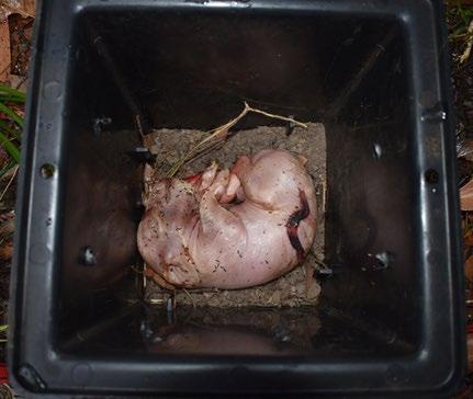
The study was conducted during autumn, it commenced on the 11th March 2019 and ran for 30 days. During the sampling procedure, replicates were observed and photographed. Sampling of adult insect fauna was conducted between 1300 and 1800 h on alternating days. Diptera were collected using an insect net and Coleoptera were collected with tweezers. All specimens were kept in sampling jars labelled with the day and replicate number. Specimens were killed at -17℃ and kept at this temperature for preservation. Gloves, goggles and organic vapour mask were used during sampling. Photographs of samples were sent to Blake Dawson, PhD Candidate University of Wollongong, for identification
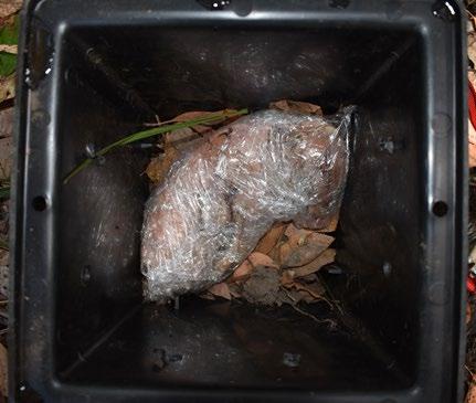 Figure 2. Wrapped piglet 1, Day 4
Figure 3. Unwrapped piglet 6, Day 4
Figure 2. Wrapped piglet 1, Day 4
Figure 3. Unwrapped piglet 6, Day 4
The Journal of Science Extension Research – Vol. 1, 2022 education.nsw.edu.au 99
Results
Table 1. DIptera and Coleoptera species succession (days) of wrapped and unwrapped carcasses
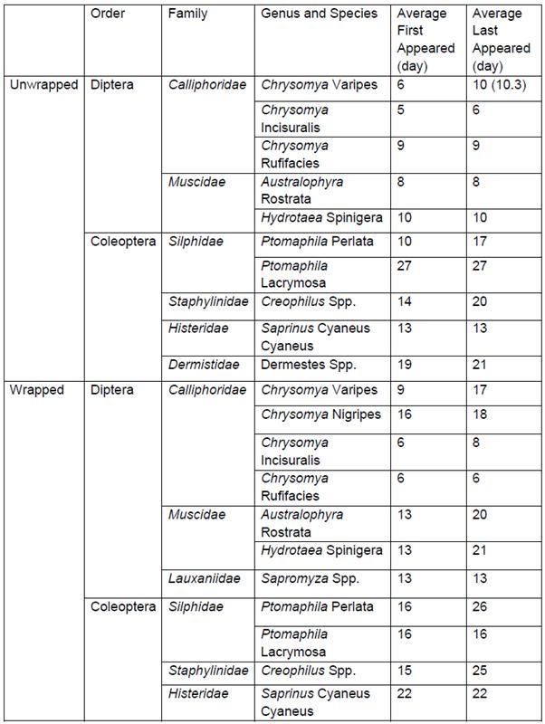
The Journal of Science Extension Research – Vol. 1, 2022
education.nsw.edu.au 100
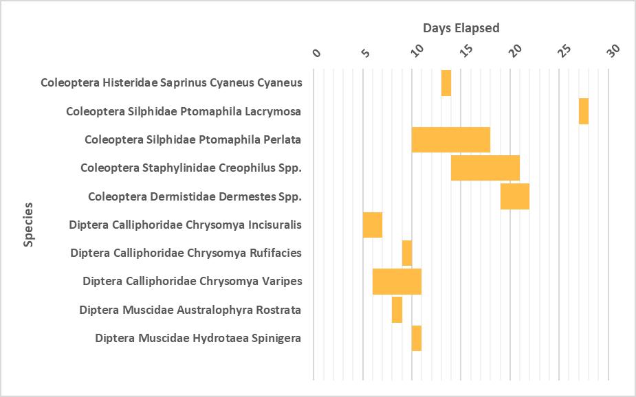
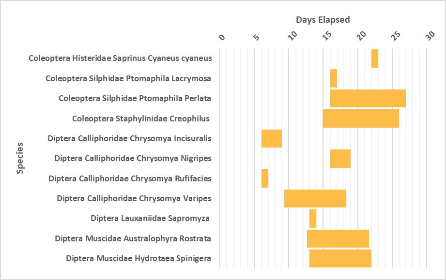 Figure 4. Coleoptera and Diptera succession of unwrapped carcasses
The Journal of Science Extension Research – Vol. 1, 2022 education.nsw.edu.au 101
Figure 5. Coleoptera and Diptera succession of wrapped carcasses
Succession
The succession patterns of Coleoptera and Diptera taxa of wrapped and unwrapped carcasses are presented above in Figures 1-2 and Table 1. Throughout this study, a total of twelve species were collected including seven of the Diptera taxa and five of the Coleoptera taxa. Specimens collected were adults; eggs, larvae and pupae were not included in this study.
Diptera Calliphoridae Chrysomya Incisuralis was the first insect to colonise both the unwrapped and wrapped carcasses. Its arrival was recorded on days 5 and 6 respectively. However, C. Incisuralis did not consistently colonise all piglets, only replicates 3 and 4. Other calliphorid colonisers included Chrysomya Varipes and Chrysomya Rufifacies, which arrived before day 10 for both unwrapped and wrapped carcasses. Diptera Muscidae
Australophyra Rostrata first colonised unwrapped replicates on day 8 and wrapped replicates on day 13. Of the Diptera taxa, Muscidae Hydrotaea Spinigera, Calliphoridae Chrysomya Nigripes (only on piglet 2) and Lauxaniidae Sapromyza Spp. (only on piget 3) were first recorded between days 9 and 16. H. Spinigera was latest Dipteran species and was last recorded on day 21 (wrapped piglet 2).
Coleoptera taxa began colonising the replicates in the later stages of the study, after the Diptera taxa, from day 9 onwards. Coleopteran colonisers included Silphidae Ptomaphila Perlata, Silphidae
Ptomaphila Lacrymosa, Histeridae
Saprinus Cyaneus Cyaneus,
Staphylinidae Creophilus Spp. and Dermistidae Dermestes Spp. These species colonised the carcasses between days 10 and 27.
Of all the species recorded, only two consistently colonised all carcasses, C. Varipes and P. Perlata. Remaining species colonised at least one wrapped and one unwrapped replicate with the exception of C. Nigripes, Sapromyza Spp. and Dermestes Spp. which only colonised piglets 2, 3 and 4 respectively.
Discussion
This study observed the impact of plastic wrapping on the succession of Diptera and Coleoptera taxa of piglet carcasses. It was evident that there were differences in the insect succession of the wrapped and unwrapped carcasses. Of the species collected, ten were observed to colonise the unwrapped carcasses before the wrapped carcasses. The length of this delay ranged from one day to nine days with an average of four days. S. cyaneus cyaneus experienced the longest delay of nine days and C. incisuralis and Creophilus Spp. experienced the shortest of one day. H. spinigera and A. rostrata experienced delays of three and five days respectively. The two predominant colonisers, C. varipes and P. perlata experienced delays of three and six days respectively. To test the hypothesis and to determine whether these differences were statistically significant, an f-test and then t-test was conducted for a number of the species. It was concluded that the delay of the above species was not significant (C. varipes: df=2, α=0.05, P=0.53). It was also observed that two of the species recorded, C. rufifacies and P. lacrymosa, colonised the wrapped
The Journal of Science Extension Research – Vol. 1, 2022 education.nsw.edu.au 102
carcasses before the unwrapped. They had a delay of -3 and -11 days respectively. Additionally, species C. nigripes, Dermestes Spp. and Sapromyza Spp. did not colonise both wrapped and unwrapped carcasses and thus did not have a period of delay.
While piglets are easily available, due to their smaller size and weight, they are not the optimal analogue for investigating human forensic entomology. Therefore, in order to better understand the effect of plastic wrapping on insect succession in relation to forensic investigations of human remains, a study must be replicated with adult pigs which are more similar to the human body, or with cadavers. It would also be beneficial to use carcasses which are the same size and weight and which have a known time and cause of death. This more controlled use of carcass is necessary for obtaining results with a higher certainty.
In this study, collection and identification of Coleoptera and Diptera taxa was limited to adults. If the collection and identification of species eggs, larvae and pupae could be performed, a more detailed view of the entomology present on wrapped and unwrapped carcasses during the stages of decomposition would be produced. Additionally, to better understand the succession of insects, specimens need to be collected daily and over a longer period of time, depending on the size of the carcasses; for example, 98 days for adult pig carcasses. The identification of specimens collected by an entomologist in person rather than through photographs would ensure the correct identification.
While it was concluded that the plastic wrapping did not significantly delay insect
succession, differences were observed between wrapped and unwrapped replicates. This may have been the result of the wrapping effecting the stages of the carcass decomposition which then had an effect on insect succession or vice versa. Other coverings such as blankets, clothes and tarps may also affect decomposition or insect succession directly. Comparing the impact of different coverings would also be beneficial to forensic entomology investigations.
The containers used in this study did not closely mimic a true crime scene and may have delayed the time that the Diptera taxa first colonised the carcasses. In the study conducted by Voss et al. (2011), it was found that Calliphora dubia Macquart (Diptera: Calliphoridae) colonised pig carcasses within the first 24 hours. In this NSW study, C. Incisuralis was the first coloniser and arrived on day 5. In order to successfully mimic a crime scene and to reduce the prevention of insect species, metal cages should be used to enclose and protect carcasses. If adult pigs or human are to be used, the bio exclusion zone should also be modified to at least 500m to meet these changes in carcass.
As the climate significantly varies throughout Australia, the results obtained from this study conducted in coastal NSW may not be entirely relevant to other parts of the country. In the investigation conducted by Voss et al. (2011), the arrival of C. dubia was significant to the study. However, in this NSW study, C. dubia was not recorded to colonise any of the carcasses at any time.
During this study, it was observed that a number of species including C. incisuralis, C. varipes, A. rostrata and Creophilus Spp. were present for longer
The Journal of Science Extension Research – Vol. 1, 2022 education.nsw.edu.au 103
periods on the wrapped carcasses compared to the unwrapped carcasses. This may be the result of the plastic limiting the evaporation of decomposition fluids which then attract the insects for a longer amount of time. It was also noted that there was an overlap of the succession of the Coleoptera taxa and Diptera taxa on the wrapped carcasses, but not on the unwrapped carcasses. This difference may be due to the wrapping prolonging the decay stage of decomposition and thus effecting the length of species succession.
Conclusion
This study aimed to answer the research question, “does the wrapping of a body delay the insect succession of Coleoptera and Diptera taxa?” Piglet carcasses were used as an analogue for human cadavers and were wrapped in plastic. C. Varipes and P. Perlata were the predominant species observed to colonise all of the carcasses. A delay of three and six days was observed for both species respectively. C. rufifacies and P. lacrymosa suggested that the wrapping did not result in a delay of the wrapped carcasses, as these species experienced delays of 3 and -11 days respectively. While the majority of the results demonstrate that there was a delay in the succession of the wrapped carcasses, it was concluded that this difference is not statistically significant (p=0.53). Thus, the null hypothesis is accepted, “Plastic wrapping of carcasses will not have an effect on Coleoptera and Diptera taxa succession.”
Acknowledgements
I thank Dr Maiken Ueland, Blake Dawson and Professor James Wallman for their advice and expertise during this study. I also thank Dr Samantha Kneeshaw and Australian Pork Ltd. for their invaluable assistance.
Reference List
Anon., n.d. [Online] Available at:
https://en.oxforddictionaries.com/definitio n/entomology
Australian Museum. 2018. Stages of Decomposition. 12 November. Accessed January 25, 2019.
https://australianmuseum.net.au/learn/sci ence/stages-of-decomposition/.
Bureau of Meteorology A. 2019. Climate Statistics for Australia locations. Accessed January 30, 2019.
http://www.bom.gov.au/climate/averages/t ables/cw_009225.shtml
Bureau of Meterology B. 2019. Climate Statistics for Australian locations
Accessed January 30, 2019.
http://www.bom.gov.au/climate/averages/t ables/cw_069138.shtml.
Cook, David, and Ian Dadour. n.d. Collecting Insects for Forensic Investigations. University of Western Australia.
Dautartas, Angela. 2009. “e E ect of Various Coverings on the Rate of Human Decomposition.” (Trace: Tennessee Research and Creative Exchange).
Joseph, Isaac, Deepu G Mathew, Pradeesh Sathyan, and Geetha Vargheese. 2011. “The use of insects in forensic investigations: An overview on the scope of forensic entomology.”
The Journal of Science Extension Research – Vol. 1, 2022 education.nsw.edu.au 104
Journal of Forensic Dental Sciences 3 (2): 89-91.
Khaliq, A., M. Javed, M. Sohail, and Muhammad Sagheer. 2014. “Environmental effects on insects and their population dynamics .” Journal of Entomology and Zoology Studies 2 (2): 17.
Oxford University Press. n.d. Entomology definition. Oxford University Press. Accessed January 7, 2019. https://en.oxforddictionaries.com/definitio n/entomology.
Schoenly, Kenneth G., Neal H. Haskell, Robert D. Hall, and Robert J. Gbur. 2007. “Comparative Performance and Complementarity of Four Sampling Methods and Arthropod Preference Tests from Human and Porcine Remains at the Forensic Anthropology Center in Knoxville, Tennessee.” Journal of Medical Entomology 44 (5): 881-894.
Vass, Arpad A. 2001. “Beyond the grave – understanding human decomposition.” MICROBIOLOGY TODAY 28: 190-192.
Voss, Sasha, Ian Dadour, and David Cook. 2011. “Decomposition and insect succession of clothed and unclothed carcasses in Western Australia.” Forensic Science International 67-75.
Zaidi, Farrah. 2017. “Use of Insect Evidence in Criminal Investigations: Developing a Framework for Strengthening of the Justice System.” Pakistan Journal of Criminology 9 (4): 111.
The Journal of Science Extension Research – Vol. 1, 2022 education.nsw.edu.au 105
Bugs on Drugs
Sidney Breth Petersen
Killarney Heights High School
This study investigates the impact of pharmaceutical drugs on the conglobation behaviour of the Armadillidium Vulgare (pill bugs). Currently, there are several studies which examine the mechanisms of this defensive behaviour, however, there are limited studies about the effects which specific drugs, such as caffeine and antihistamine, could have on this mechanism. This study compares the conglobation time of pill bugs who consumed purely water, to ones which consumed diluted solutions of pharmaceutical drugs. Results revealed that pill bugs which were exposed to the caffeine solution had significantly higher conglobation times. This proposes that caffeine induced water loss in pill bugs which caused them to conglobate. Similarly, the antihistamine group also had an increased conglobation time, but the increase was to a lesser extent. This increase may be impacting the defensive aspect of the conglobation mechanism, as central nervous system activity could have been slowed due to the sedative behaviour of antihistamines. Both drug classes impacted upon the conglobation behaviour of the pill bug which suggests that drugs polluting water sources in pill bug habitats could be placing stresses on the species and threaten their survival.
Literature Review
Worldwide, pharmaceutical compounds are traced in the aquatic environment. This exposure to pharmaceuticals has led to ecotoxicological effects on various species. Previous experiments have aimed to explore the effect of various drug classes on animals to examine the ways in which they affect the nervous system. By examining the effect of these drugs, the harmful impact of drugs in grey water can be examined and potentially limited if they pose harmful effects to species. Different drug classes affect the central nervous system (CNS) in various ways (NIDA, 2020). Typical pharmaceutical compounds which have an effect on the CNS are antihistamines and caffeine. Pill bugs are terrestrial arthropods which are sensitive to the
amount of water present in their environment.
The effects of these two different drug classes have been closely examined in humans and other animals, but research is lacking on their effects on pill bug activity. In humans, antihistamines are a CNS depressant, whereas caffeine is a stimulant. Neither are harmful to humans in small doses but their effect on pill bug activity has not been examined extensively. A lack of evidence exists regarding isopod metabolism, particularly the physiological mechanisms of drug metabolism in the pill bug. Whilst a large body of literature exists regarding the cytochrome P450 enzyme in mammalian metabolism, there is a lack of knowledge on isopod metabolism.
The Journal of Science Extension Research – Vol. 1, 2022 education.nsw.edu.au 106
It is crucial to understand how these drugs work in order to understand how they would affect the functionality of pill bugs. Caffeine, besides influencing cognitive performance, increases the perception of alertness, wakefulness and can induce anxiety (Cappelletti, 2015). Caffeine stimulates antagonists against adenosine receptors within the CNS (Ribeiro, J. A., & Sebastião, A. M., 2010) which prohibits cells from identifying adenosine, an indicator of fatigue. This means the brain becomes non-perceptive of fatigue. In addition, caffeine promotes diuresis, the excretion and loss of water from the body. These two effects have been thoroughly studied, yet there is a lack of literature which investigates the dangers this poses to pill bugs which are dependent on water for survival.
Histamine is a CNS neurotransmitter which is necessary in maintaining wakefulness, alertness, and reaction time (Lieberman P., 2009). This wakefulness can be impaired by antagonists, known as antihistamines. In addition to their potent activity in histaminergic pathways, first generation antihistamines also demonstrate a significant degree of pharmacologic activity in α-adrenergic pathways. Most commonly, the cognitive impairment associated with diphenhydramine is due to the αadrenergic blockade. This means, in comparison to caffeine, the drug may cause physiological changes such as decreased movement speed and activity, if they have similar effects in pill bugs.
Pill bugs are relatively poorly adapted to land, and can only survive habitats where temperatures are moderate and damp surfaces are available (Jacob T. Smigel and Allen G. Gibbs, 2009). Evaporation from the outer surface is the most
important physiological factor affecting their survival. However, pill bugs are capable of conglobation which is the process of rolling into a ball. This behavior, other than acting as protection from predators, also protects the more delicate ventral surface, allowing pill bugs to survive in harsh conditions by reducing water loss.
A journal article published in 2008, (Jacob T. Smigel and Allen G. Gibbs)
‘Conglobation in the Pill Bug, Armadillidium vulgare, as a Water Conservation Mechanism’ examined the conglobative behavior of pill bugs as a possible water conservation mechanism. Evidence found, demonstrated that pill bugs spontaneously conglobate at 40°C, with a resulting decrease in their rates of water loss. Pill bugs were found conglobated in dry soil, and unconglobated in visibly moist soil, suggestive of water conservation methods. To test this hypothesis, the water loss rate of unconglobated and conglobated isopods were measured. The data showed that conglobation significantly reduced water loss by 34.8%, suggesting that conglobation behavior may help to conserve water.
Previous studies have reported findings that certain drugs, such as caffeine, can have harmful effects on both humans and animals (P. N. Witt, 1948), such as examining the effects of psychoactive drugs on spiders. The study conducted by Witt (1948) concluded that relatively small doses of many different drugs affect the pattern of a spider web. In support of these findings, it was also examined that caffeine may function as a natural insecticide and hence may be useful in insect control (J. A. Nathanson).
Subsequently, research by the National
The Journal of Science Extension Research – Vol. 1, 2022 education.nsw.edu.au 107
Aeronautics and Space Administration
(NASA) in 1995 tested the effect of various other drugs in order to build on previous findings. The study allowed NASA to conclude that several drugs can impact spider activity by affecting the CNS.
Although we cannot link drug effects on pill bugs to drug effects on humans, we can examine through primary research, how pharmaceuticals such as caffeine and antihistamines in pill bug habitats, can cause severe impacts. This is due to the nature of caffeine and antihistamines influencing central nervous system activity.
Scientific Research Question
What are the effects of different drug classes on conglobation behaviour of the pill bug, Armadillidium vulgare?
Scientific Hypothesis
Caffeine will act as a diuretic on the pill bug, causing water loss, and will therefore increase conglobation time. Antihistamines will not have a significant effect on the conglobation period of pill bugs, but may still cause slight increase in conglobation time.
Methodology Drugs
The antihistamine, Dexychloropheniraminemaleate
(50mg/1ml, 1g of Dexchlorpheniramine in 20ml of water) and caffeine solution
(50mg/1ml, 1g of Caffeine Anhydrous in 20ml of water) were purchased from Pittwater Pharmacy & Compounding
Chemist and kept in small spray dispensers.
Pill bugs
100 pill bugs were collected from their natural environment and stored in containers. These containers had controlled environments, with the same type of soil, food and light availability and temperature, in each container. Hence, variables such as amount of water present, which had inevitable variations, could be controlled.
Filter paper and petri dishes
The soaked filter paper was prepared by spraying the filter paper five times each with the drug solutions. Each spray with the drug solution dispenses 0.1mL of liquid, meaning that each filter paper was soaked in 0.5mL of the selected solution. Each time a petri dish was lined with the soaked filter paper, a label was attached clearly indicating which drug was being used (Figure 1).
Drug administration
When conducting the experiment, pill bugs were placed into three groups: a petri dish environment with either water, caffeine or antihistamine. 10 specimens were placed in each group. The time the pill bugs were placed on the petri dish was clearly recorded. The pill bugs were then left in the petri dishes for 30 minutes before being removed.
Recording the effects of various drug classes on conglobation rates
As soon as the pill bugs were removed, they were kept in their groups and placed on separate dry pieces of paper. A new timer was then started to record the time taken for the pill bugs to open up and start moving around, and these results were recorded in a table which was then
The Journal of Science Extension Research – Vol. 1, 2022 education.nsw.edu.au 108
analysed based on the differences between the conglobation rates of each drug class. Statistical T-test was then conducted to compare the means between each group, comparing the two different drugs to water, allowing us to reject or accept hypotheses and evaluate whether or not there is statistical difference between the two selected data sets.
The length of the conglobation time post drug administration was recorded for each individual pill bug and the average time of the test group was taken. Table 1 indicates the length of conglobation time post drug administration for each individual pill bug in the first two study groups, as well as the average time of each test group. The mean conglobation time for study groups 1 and 2 were 220.4 and 262.6, respectively.
The averages for each drug class were recorded (table 2, figure 2). For the conglobation time, note that caffeine administration results significantly increased time under conglobation. That is, there was an increase of 223.22 seconds between the caffeine and water group.
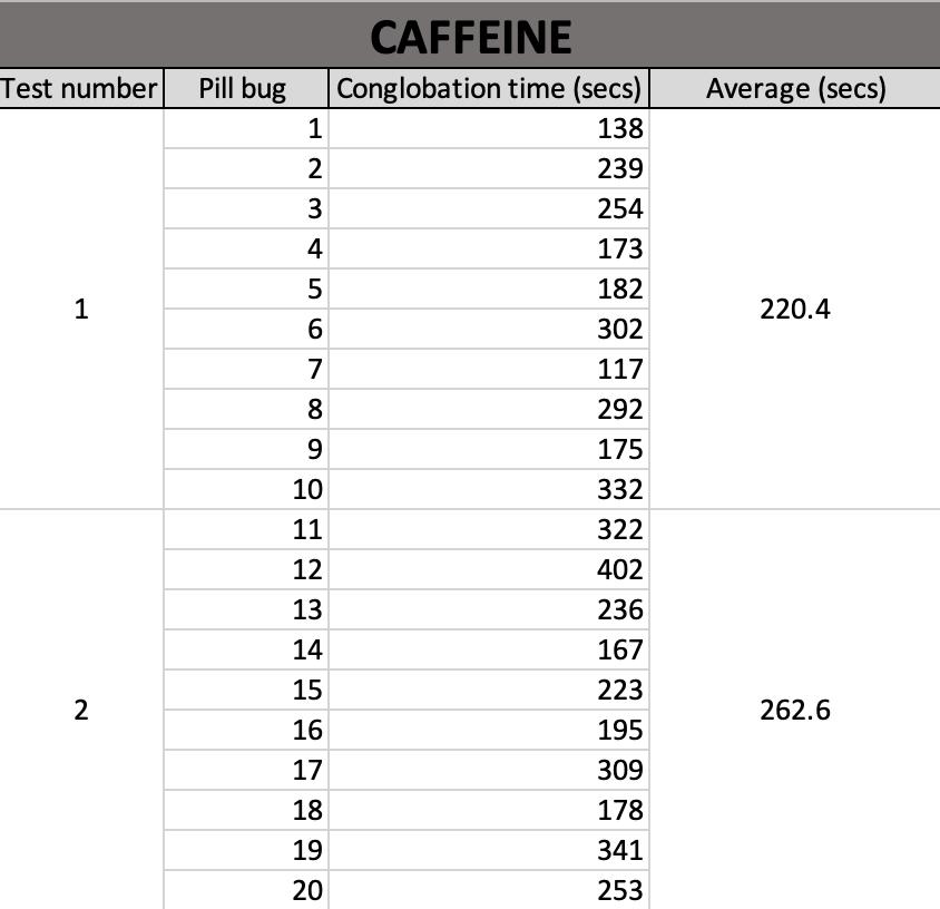
An increase in conglobation time was also observed in the antihistamine group (table 2) which shows an increase of 15 seconds between the respective antihistamine and water group.
Results
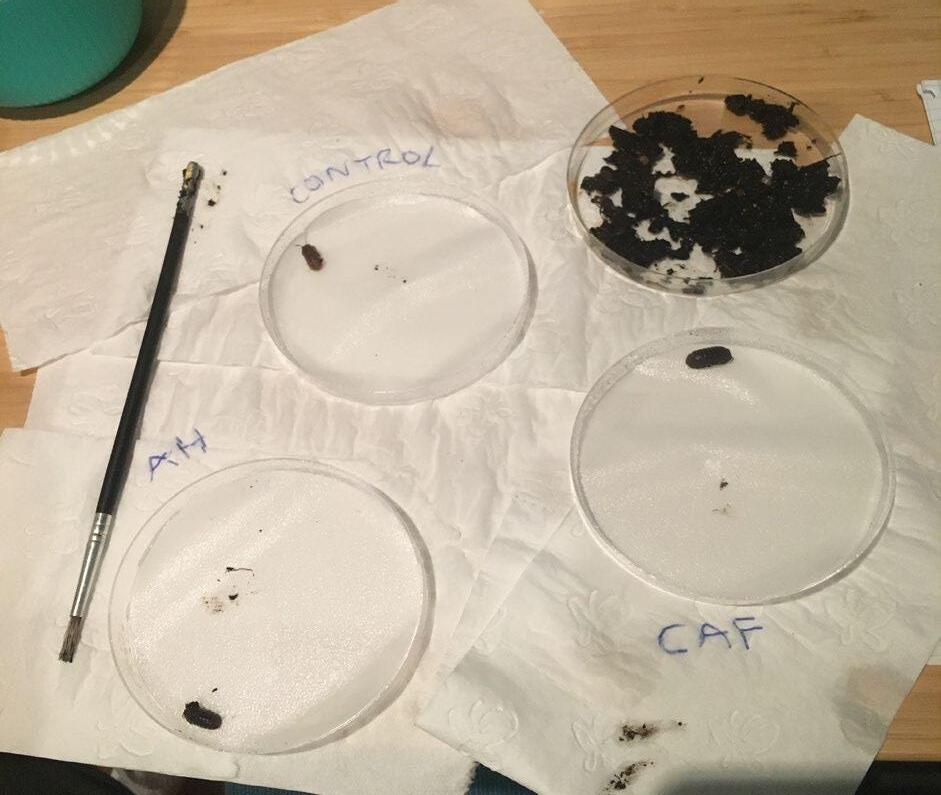 Figure 1) Example petri dishes with soaked filter paper
Table 1) Results of the first two caffeine groups
Figure 1) Example petri dishes with soaked filter paper
Table 1) Results of the first two caffeine groups
Drug class Average conglobation time over all tests Caffeine 244.97 Antihistamine 36.75 water 21.75 The Journal of Science Extension Research – Vol. 1, 2022 education.nsw.edu.au 109
Table 2) Average conglobation time of each drug class administered.
A two-tailed t-test was conducted with an alpha value of 0.05 (table 6). The results showed that the water conglobation time was less than the caffeine conglobation time, and found a significant difference between the two means as the P-value was less than 0.05. This indicated that there is a statistical difference between the two means, and allows us to reject the null hypothesis that there was no
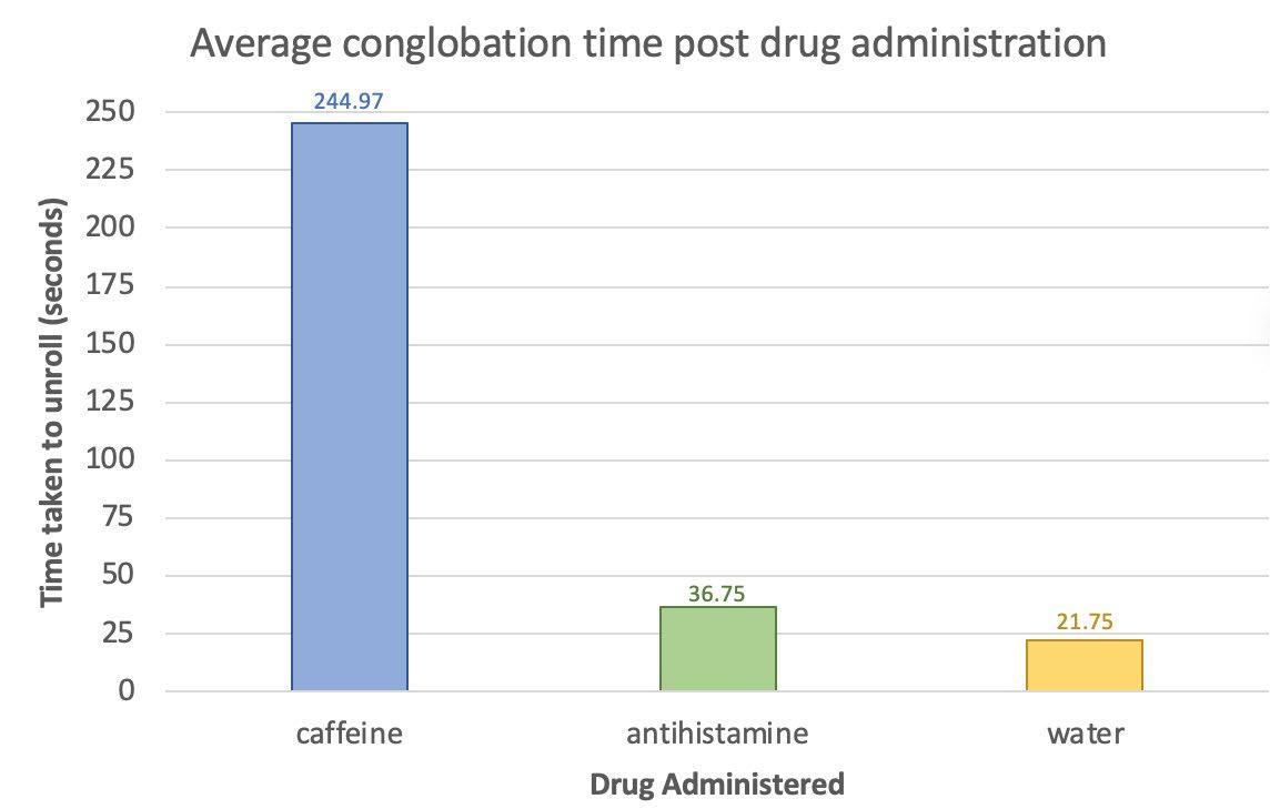
statistical difference between the caffeine group and the water group.
An identical test was conducted between the mean of the antihistamine group and the water group with a P-value less than 0.05, suggesting there is significance in the results and allows us to reject the null hypothesis that there was no statistical difference between the antihistamine group and the water group.
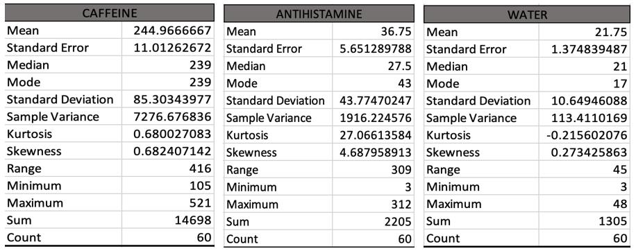 Figure 2) Average conglobation time of each drug class administered
Table 3) descriptive statistics of results
Figure 2) Average conglobation time of each drug class administered
Table 3) descriptive statistics of results
The Journal of Science Extension Research – Vol. 1, 2022 education.nsw.edu.au 110
There is a large difference between the two t-tests result, with the P value of the caffeine group being significantly smaller than the antihistamine group. This is due to the time increase of conglobation which was observed, as the antihistamine group did not have as large of an increase as that of caffeine.
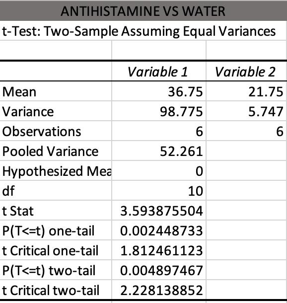
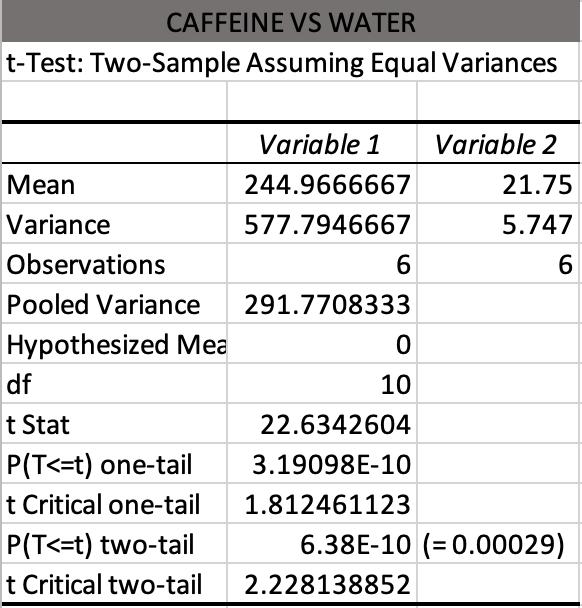
Discussion
Administration of caffeine in pill bugs significantly increased the conglobation time of pill bugs (table 2). In comparison, antihistamines had very little effect on the conglobation time, however still saw an increase.
Both tests have been able to find significant differences in conglobation time after caffeine and antihistamine were administered, and suggest that the test hypothesis can be accepted.
The caffeine group results (seen in table 2), suggests that caffeine increased the conglobation time of pill bugs, which may be related to the diuretic nature of caffeine. This demonstrates the correlation between the nature of caffeine as an inducer of water loss (Stookey, J.), and the conglobation behaviour of pill bugs as a means of water conservation (Jacob T. Smigel and Allen G. Gibbs ), suggesting that caffeine acts as a diuretic in pill bugs, as it does in humans.
Water loss is important to protect pill bugs. If caffeine causes loss of H+ ions and acts as a diuretic (Maughan, R. J., & Griffin, J.), it would pose a threat to the survival of a species, which is exposed to caffeine, as they cannot survive without a sufficient amount of water. This highlights the severe effects which caffeine entering pillbug environments could have on pill bug colonies. These findings could help to examine the dangers of grey water in pill bug habitats, as pill bugs survive from the moisture in the soil, including any grey water that has entered the habitat.
The slight increase in conglobation time seen in the antihistamine group may result from the sedative effect of antihistamine. This effect could have
Table 6) T-Test results, comparing the means between the caffeine and water results
Table 7) T-test results, comparing the means between the antihistamine and water results
The Journal of Science Extension Research – Vol. 1, 2022 education.nsw.edu.au 111
slowed down the pill bug response times to stress and cause the increased mean conglobation time (graph 1). It is possible that the antihistamine group had a longer conglobation time than the water group, as the drug caused physiological changes such as decreased movement speed and central nervous system activity.
Each pill bug was obtained from their natural habitats but from various locations. They were all of different sizes and some even of different colour. This could be due to age or the environmental conditions, which were not taken into account when observing the effects of the drugs. If the pill bugs obtained were of the same size, this would increase the amount of controlled variables as the experiment does not observe whether or not the variance within the drug groups were due to size differences. Changes in size could increase the surface area of the bug, exposed to evaporation and hence increasing the rate of water loss. These variables were partially controlled by using a large sample size. Other variables which had inevitable variations that could have affected the rate of water loss and the effect of the drug also includes the amount of food and water they were obtaining prior to the drug administration. To minimise the effects of these factors, each pill bug habitat was sprayed with the same amount of water daily and ensured each enclosure has the same level of food availability.
There were also ethical concerns with testing on the pill bugs which need to be considered through all areas of study. Within this study, five pill bugs were tested prior to the thorough experiment conducted, to ensure that the effects observed were only temporary and did not affect survival.
The measurement of drug responses also needed to be carefully considered. A journal article (Jacob T. Smigel and Allen G.Gibbs) on conglobation measured changes in metabolic rate and water-loss rate using a flow-through respirometry chamber, which if able to be utilised in a similar investigation, could accurately measure how drug administration changes metabolic and water-loss rate. This equipment measures respiration rates of living organisms, which allows investigation into how factors such as age, or chemicals affect the rate of respiration. The major route for water loss in pill bugs is evaporation from the body surface, particularly the respiratory organs. By having a respirometry chamber, it would limit experimenter bias as to whether the drug itself is causing certain effects or other factors. Instead, the experiment conducted utilised a visual analysis and time to record changes to conglobation behaviour, which could be backed up by quantitative evidence of the changes in water loss that caffeine causes. Access to this technical equipment would be able to certify that the changes are due to the diuretic nature of caffeine and not the psychological effects that it presents to the consumer.
Further suggestions
Coffee grounds are often used in gardens to promote plant growth, which is another way that caffeine can enter habitats. Further research could include investigating the variety of organisms in soils where coffee grounds have been added, in comparison to areas where there were no coffee grounds used.
If the drug contamination levels currently present in various pill bugs habitat were obtained, these amounts of caffeine and
The Journal of Science Extension Research – Vol. 1, 2022 education.nsw.edu.au 112
antihistamine could be used in the experiment as this will be a more accurate indicator of the threat which soil contamination presents to pill bugs. This experiment assumes that the levels of pharmaceuticals in the soil are directly impacting the pill bugs as they are exposed to similar levels, however levels may be significantly lower or higher. In addition, if the amount present in soil is in fact higher than what was used in the experiment, this could pose an additional threat to pill bugs, as it has now been discovered that naturally occurring amounts of caffeine kill several animals, including pill bugs (Nathanson J. A.). Further studies should also investigate whether increasing moisture would mitigate the harmful effects of caffeine.
It should also be identified that we cannot assume from this paper that there is a correlation between what a drug does to the conglobation mechanisms in the pill bugs brain, and what they do to human brains. Rather, we should use it as an indication as to where similarities in drug behaviour lie and how they may affect species differently.
Conclusion
Pill bugs are sensitive to the amount of water present in their environment and have therefore adapted mechanisms such as conglobation to reduce water loss. The results of this study suggest that there was a statistically significant difference in the conglobation time of the caffeine group and antihistamine group in comparison to the pill bugs who were only exposed to water. The investigation specifically revealed that the increase in conglobation time for the caffeine group was much higher than the antihistamine group, although as hypothesised, both
drugs affected the conglobation mechanism.
Further research should be conducted which examines the specific amount of water lost due to caffeine administration and consider the effects of varying caffeine concentrations. Utilising the concentration of caffeine that can be found in grey water, near pill bugs, should also be examined on its effects as this would allow for more detailed analysis of the severity of grey water effects. By conducting further research on how pill bugs metabolise drugs it could be examined whether they have a compound that may limit or enhance the efficacy of certain drug types.
Reference List
Cappelletti, S., Piacentino, D., Sani, G., & Aromatario, M. (2015). Caffeine: cognitive and physical performance enhancer or psychoactive drug? Current neuropharmacology, 13(1), 71–88.
Church, M. K., & Church, D. S. (2013). Pharmacology of antihistamines. Indian journal of dermatology, 58(3), 219–224.
Fran M. Gengo, PharmD, (DECEMBER 01, 1996) Reduction of the central nervous system adverse effects associated with antihistamines in the management of allergic disorders: Strategies and progress, FCP VOLUME 98, ISSUE 6, PS319-S325
Hansen, L.L., Westh, P. Wright, J.C., and Ramløv, H. 2006. Metabolic changes associated with water vapour absorption in the mealworm Tenebrio molitor L. (Coleoptera: Tenebrionidae): a microcalorimetric study. Journal of Insect Physiology 52, 291-299.
The Journal of Science Extension Research – Vol. 1, 2022 education.nsw.edu.au 113
Hindmarch, I. (2002), CNS effects of antihistamines: is there a third generation of non‐sedative drugs? Clinical & Experimental Allergy Reviews, 2: 26-31.
Koh, H. and Wright, J.C. 2011. Cation regulation by the terrestrial isopod Armadillidium vulgare (Crustacea: Isopoda: Oniscidea) during dehydration in air. Comparative Biochemistry and Physiology A, 159(2), 134-140.
Lieberman P. (2009). Histamine, antihistamines, and the central nervous system. Allergy and asthma proceedings, 30(5), 482–486.
Maughan, R. J., & Griffin, J. (2003). Caffeine ingestion and fluid balance: a review. Journal of human nutrition and dietetics : the official journal of the British Dietetic Association, 16(6), 411–420.
Matsuno, H., & Moriyama, T. (2012). Behavioural evidence for internal factors affecting duration of conglobation in pill bugs (Armadillidium vulgare, Isopoda, Crustacea). Short communication. Acta biologica Hungarica, 63 Suppl 2, 80–82.
Meltzer E. O. (1990). Performance effects of antihistamines. The Journal of allergy and clinical immunology, 86(4 Pt 2), 613–619.
Moriyama, Tohru (2004) Problem Solving and Autonomous Behavior in Pill Bugs (Armadillidium vulgare), Ecological Psychology, 16:4, 287-302.
Moriyama, T. (1999). Decision-Making and Turn Alternation in Pill Bugs ().
Nathanson J. A. (1984). Caffeine and related methylxanthines: possible naturally occurring pesticides. Science (New York, N.Y.), 226(4671), 184–187.
NIDA. 2020, July 10. Drugs and the Brain. Retrieved on 2020, July 26
Ribeiro, J. A., & Sebastião, A. M. (2010). Caffeine and adenosine. Journal of Alzheimer's disease : JAD, 20 Suppl 1, S3–S15.
Schlüter, U., & Seifert, G.D. (1985). Functional morphology of the hindgutMalpighian tubules complex in Polyxenus lagurus (Diplopoda; Penicillata).
Smigel, J. T., & Gibbs, A. G. (2008). Conglobation in the pill bug, Armadillidium vulgare, as a water conservation mechanism. Journal of insect science (Online), 8, 1–9.
Stookey, J. (1999). The Diuretic Effects of Alcohol and Caffeine and Total Water Intake Misclassification. European Journal of Epidemiology, 15(2), 181-188. Retrieved July 8, 2020
Sturman G. (1996). Histaminergic drugs as modulators of CNS function. Pflugers Archiv : European journal of physiology, 431(6 Suppl 2), R223–R224.
Toru Moriyama, Masao Migita, Meiji Mitsuishi, Self-corrective behavior for turn alternation in pill bugs (Armadillidium vulgare), Behavioural Processes, Volume 122, 2016, Pages 98-103, ISSN 03766357.
Welch W. J. (2015). Adenosine, type 1 receptors: role in proximal tubule Na+ reabsorption. Acta physiologica (Oxford, England), 213(1), 242–248.
Witt, P.N. (1971), Drugs alter web‐building of spiders: A review and evaluation. Syst. Res., 16: 98-113
The Journal of Science Extension Research – Vol. 1, 2022 education.nsw.edu.au 114
Witt, P., & Reed, C. (1965). Spider-Web Building. Science, 149(3689), 1190-1197.
Retrieved July 8, 2020
Wright, J.C., and Machin, J. 1993. Atmospheric water vapour absorption and the water budget of terrestrial isopods. Biological Bulletin 184, 243-253.
Wright, J.C., and O’Donnell, M.J. 1995. Water vapour absorption and ammonia volatilization: adaptations for terrestriality in isopods. pp 25-45 in M.A. Alikhan (Ed.) Terrestrial Isopod Biology (Crustacean Issues 9). A.A. Balkema, Rotterdam.
The Journal of Science Extension Research – Vol. 1, 2022 education.nsw.edu.au 115
Call for submissions
For the opportunity to have your students' research reports showcased in the next edition of the Science Extension journal, contact the Science 7-12 curriculum team.

Contact Science 7-12 curriculum team Science7-12@det.nsw.edu.au
NSW Department of Education