Characterisation of the Chaotic Behaviour of a Simple TwoTransistor Single-Supply Resistor-Capacitor Circuit

Characterisation of the Chaotic Behaviour of a Simple TwoTransistor Single-Supply Resistor-Capacitor Circuit

James Harrison – Lambton High School

Abstract

The claims of chaotic behaviour in the circuit proposed by Keuninckx et al. (2015) were investigated through utilising both in-situ and in-silico solutions. The circuit’s behaviour was characterised in two modes, depending on the location of the variable resistor, with the resistance range of chaotic behaviour observed within each mode varying between modes. Chaotic behaviour in both modes of the proposed circuit was found through the calculation of positive Lyapunov exponents across the range of resistances studied from simulation data. The validity of the simulation was confirmed as chaotic behaviour was observed for each mode in the in-situ circuit. Therefore, the claims of Keuninckx et al. (2015) were confirmed. The proposed chaotic circuit utilised cheap and readily available parts, hence, there is scope for its implementation in areas such as robotics or encryption, where chaos greatly increases efficiency and effectiveness.

Literature Review

Chaos theory is a mathematical theory which states that in dynamic systems displaying apparent randomness, there is underlying order within this apparent randomness. The theory involves the idea that chaotic systems are deterministic which means that, in principle, the future state of a system can be predicted mathematically (Oestreicher, 2007). However, this means that these systems are extremely sensitive to initial conditions, making it extremely difficult to predict the long-term state of these systems. The concept of chaos has been observed and articulated throughout human history, as evidenced by attributions to Aristotle, who observed that “the least initial deviation from the truth is multiplied later a thousandfold” (Aristotle, OTH). However, it was not until Edward Lorenz investigated chaotic behaviour in weather patterns when interest in the study of chaotic systems exploded (Bishop, 2017). In 1961, Lorenz noticed that rounding to 3-digits during a meteorological calculation meant that the result greatly diverged from the results obtained when rounding to 6-digits (Oestreicher, 2007), discovering the idea of deterministic chaos. This laid the groundwork for chaos theory to exist, enabling the subsequent explosion of interest and research into the topic that has allowed for a deeper understanding of how chaos impacts human lives and how it can be used in real-world applications.

When describing chaotic systems, one thing to note is that a complex system does not imply a chaotic system and, likewise, a chaotic system is not always complex (Rickles et al., 2007). Complex systems involve many interactions between subunits whilst simple systems involve only a few interactions between subunits which behave according to simple laws. A chaotic system can be simple, with only a few subunits, which interact to create chaotic dynamics, with Sprott (1994), noting that chaos can surprisingly occur in very simple nonlinear equations. The study of chaos in simple systems is of particular significance, as it may have implications in many fields which deal in simple systems and yet experience chaotic behaviour. In the case of this investigation, the electronic circuit is an example of a simple system, as there are a limited number of well-defined components that make it function, however, it still will display chaotic behaviour because of the non-linear dynamics which govern it.

There is a need for flexible, low-cost chaotic systems based around electronic circuits because a variety of applications, such as robotics and encryption, are emerging which can utilise chaos in order to be more effective (Tanougast, 2011). An application which could utilise chaos theory is that of encryption. Chaotic encryption would be significantly harder to decrypt by brute force, and providing the idea of deterministic chaos holds true, would allow for the desired user to easily access the information if they have access to an encryption key outlining the initial conditions of the system. One area of encryption which could utilise chaos theory is image encryption, detailed by Shaukat et al. (2020). Chaotic properties of complex dynamics, deterministic behaviours, ergodicity, pseudorandomness, high sensitivity to initial conditions, etc. allow for the creation of a more secure encryption method. The use of these chaotic properties allows for a highly random sequence to be generated based on a chaotic system, instead of the classical algorithm, which allows for a more secure and efficient image encryption method over conventional techniques. Shaukat et al. (2020) propose several recommendations for future research and development of image encryption utilising chaos theory; the most notable of these is the need for practical and feasible methods of generating chaotic dynamics, as many proposed methods have extensive hardware requirements due to computational complexities. This could be addressed through continued research and application of chaotic circuits constructed from simple and low-cost components, both in their physical form and simulated software form. Similarly, the use of chaotic circuits in robotics may also greatly improve the functionality of these systems. The current autonomous robotic solutions are limited in their behavioural patterns, however, through the use of a chaotic system, the potential number of behavioural patterns can be increased for these autonomous robots (Steingrube et al., 2011).

The first chaotic circuit proposed and created was by Leon Chua who mathematically determined and designed a circuit which displayed chaotic behaviour. Chua’s circuit (shown in Figure 1) was incredibly simple, consisting of an inductor (L), two capacitors (C1 and C2), a linear resistor (R) and a negative non-linear resistor (NR), and it is simply this non-linear resistor which makes the circuit chaotic, as the other four are linear elements (CHAOTIC CIRCUITS, 2015) This simple design has paved the way for the development of most chaotic circuits, either by adding elements to increase their chaotic behaviour or using similar mathematical ideas to put into circuital implementation. However, many of these circuits, including Chua’s circuit, utilise complex components (such as inductors, analogue multipliers, or operational multipliers) in order to display chaotic behaviour, which is not necessarily disadvantageous within itself, but avoiding such elements would be beneficial in terms of cost and circuit complexity. This would also simplify the ability to model such circuits through software simulation which would allow chaotic behaviours to be more easily integrated into applications. Furthermore, there is no correlation between the use of these complex components and the degree to which the circuit displays chaos, therefore, if an effective simple circuit using readily available parts was developed, this would be more desirable from a cost and logistics stand-point (Keuninckx et al., 2015).

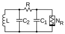
Figure 1. Chua’s Circuit

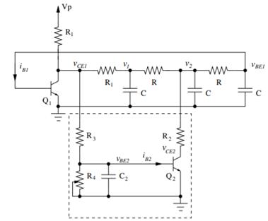
Keuninckx et al. (2015) proposed a simple two-transistor single-supply resistor-capacitor chaotic oscillator where the circuit designed utilises a transistorbased RC-ladder with a small onetransistor subcircuit directly attached to this RC-ladder (represented by the dashed box in Figure 2), adding a new equilibrium to the system in which Q1 also is biased as an active amplifier, enabling chaotic oscillations and behaviour. Therefore, as there are no complex components, the advantage of this circuit lies in its simplicity because it is much easier to model mathematically (as it is less straightforward to integrate circuits containing elements such as inductors) and it is much more cost effective, as well as easier to construct, due to a low parts count (Keuninckx et al., 2014). The circuit is also described by four relatively simple differential equations (Figure 3), which means that the state of the system at a given point can be easily determined mathematically. Furthermore, neither the values for the components nor the supply voltage are critical, and the frequency range is scalable (Keuninckx et al., 2015); the implications of this circuit design are that it can be utilised and adapted into a variety of applications which could take advantage of chaos, such as image encryption or robotics.

Figure 2. A simple two-transistor singlesupply resistor-capacitor circuit

(Keuninckx et al., 2015).

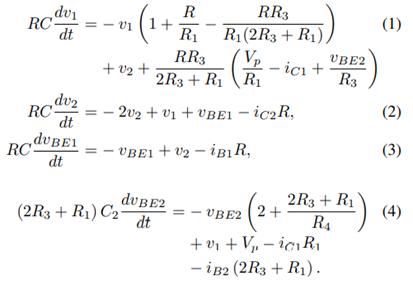
Figure 3. Differential equations which describe the circuit in Figure 2

(Keuninckx et al., 2015).

Scientific Research Question

The investigation will model and experimentally confirm the chaotic behaviour in a simple two-transistor single-supply resistor-capacitor chaotic oscillator with the aim of confirming the claims by Keuninckx et al. (2015) that two circuit layouts, where the location of the variable resistor is switched between R3 and R4, of chaotic behaviour can be observed with this circuit design.

Scientific Hypotheses

H0: If the position of the variable resistor (R4) within the circuit is changed, then the circuit will not display chaotic behaviour in this new circuit layout across the range of resistances studied.

HA: If the claim by Keuninckx et al. (2015) is true, then when the position of the variable resistor R4 within the circuit is changed to the position of R3 (and R4 is replaced by the resistor R3), then the circuit will continue to display chaotic behaviour in this new circuit layout, evidenced by generating positive Lyapunov exponents, across the range of resistances studied.

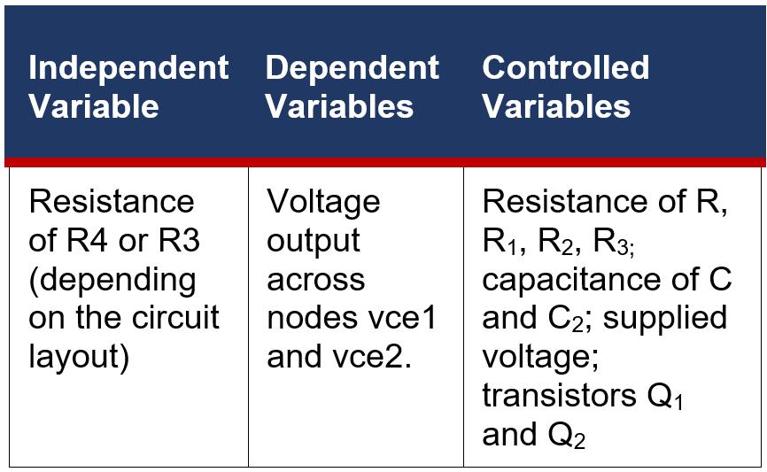
Variables

Methodology

Part 1: Circuit Design and Physical Construction

The physical circuit was constructed on a breadboard, shown in Figure 4, based on the circuit design of Keuninckx et al. (2015), shown in Figure 5. Off-the-shelf physical components for the circuit were sourced Core electronics and element14. The resistances of a few resistors were slightly changed as resistors with their exact resistances were not readily available. These differences in resistance were not very significant and are attributed to rounding and generalisation by Keuninckx et al. (2015). Figure 4 shows the completed circuit on the breadboard in Mode 1, the primary design reported by Keuninckx et al. (2015), where the variable resistor is located at R4 and a fixed resistor at R3. While Mode 2 has the variable at R3 and the fixed resistor located at R3.

Part 2: Software experimentation using LTSpice

In order to obtain data which can be analysed using TISEAN software (Hegger et al., 1999), the platform LTSpice was utilised. It is not feasible using the equipment and technology available for this research to collect specific data points in a physical model of the circuit across a 20ms timestamp, hence a LTSpice simulation of the circuit was used. Using LTSpice, the Mode 1 circuit proposed by Keuninckx et al. (2015) was created, shown in Figure 6, and simulations were run for varying resistances of R4. Voltage measurements were taken across the nodes vce1 and vce2 to monitor the chaotic behaviour of the circuit. These graphs can be compared to the output graph of the oscilloscope produced by the physical circuit in order to confirm the validity of the simulation. One output which should display chaos is the voltage across the node vce1, according to Keuninckx et al. (2015), therefore, voltage readings across this node was taken across a 20ms time period (as shown in the in-silico vce1 vs. time data given in in Figures 7 and 8). This data was generated for integer resistances of R4 between 35kΩ and 75kΩ to show the range of resistances where chaos is generated. This was then repeated for the circuit in Mode 2 (with integer resistance between 15kΩ and 70kΩ), with the resistance of R3 being changed and the resistance of R4 kept constant at 40kΩ. The data was then analysed using the TISEAN software to calculate Lyapunov values where chaotic voltages were observed.

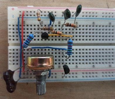
Figure 4. The circuit shown is physically made on a breadboard with R4 as the variable resistor (mode 1).

Figure 5. A simple two-transistor singlesupply resistor-capacitor circuit. The components have the following values: R = 10kΩ, R1 = 5kΩ, R2 = 15kΩ, R3 = 30kΩ, C = 1nF, C2 = 360pF, and VP = 5V.

(Keuninckx et al., 2015)

Part 3: Conducting the practical experimentation

The goal of the practical experimentation using a physical circuit on a breadboard was to confirm the results obtained from the software simulation in order to demonstrate the validity of the data obtained from this simulation. An oscilloscope (QC1932 Digitech Digital Oscilloscope) was used to obtain the results of the physical circuit which produced a graph of voltage versus time across vce1 and vce2. Due to limitations of the oscilloscope, traces for the oscillations in voltage across the node vce1 could not be clearly seen so only oscilloscope traces for voltage across the node vce2 versus time were obtained.

Conducting data analysis using TISEAN

The TISEAN analysis package (Hegger et al., 1999) was used to analyse and quantify the non-linear behaviour observed in this study; the function of calculating the maximal Lyapunov exponent was used in order to demonstrate whether or not chaos occurs in the circuit at a variety of resistance in both modes of the circuit. The Cygwin platform was utilised to run the TISEAN analysis package. The ‘lyap_k’ function from the package was used to calculate the suite of Lyapunov exponents which uses the Kantz algorithm (Kantz, 1994).

Results

Physical Validation of Simulation:

A comparison of the in-situ experiment with a voltage probe on vce2 measuring voltage and the in-silico experiment with voltage measured across vce2, shown in Figures 7 and 8, show that chaos is exhibited in both modes in the physical circuit. This chaos is shown by the erratic, inconsistent signal produced which draws similarities to that of the in-silico simulation. While the in-situ graph displays slight discrepancies of spikes in voltage, these are most likely caused by minor variations in component performances and limitations associated with the oscilloscope to measure the small voltage fluctuations observed. An adjustment of the variable resistor in each circuit showed chaos exhibited across a variety of resistances in both in-situ and in-silico circuits.

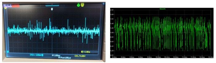
Figure 7. Mode 1; right – in-situ oscilloscope display (voltage vs. time); left – in-silico voltage vs. time plot

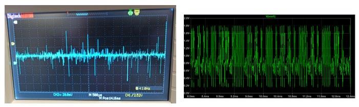
Figure 8. Mode 2; right – in-situ oscilloscope display (voltage vs. time); left – in-silico voltage vs. time plot

Visual Analysis of LTSpice Simulation:

When voltage across nodes vce1 and vce2 (in Mode 1 and Mode 2) are plotted against each other the graph of the chaotic attractor shown in Figure 9 and 11 is produced, which shows bistable oscillations around two unstable equilibria, indicative of the chaotic behaviour of the circuit. Similarly, when voltage across nodes vce1 and v1 are plotted against each other in Figure 10 and 12, this same chaotic attractor of oscillations around two unstable equilibria can be seen.

Figure 9. vce1 vs. vce2, for R4 = 40kΩ Figure 10. vce1 vs. v1, for R4 = 40kΩ

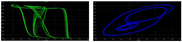
Figure 11. vce1 vs. vce2, for R3 = 24kΩ Figure 12. vce1 vs. v1, for R3 = 24kΩ

Summary of Results:

Figures 13 and 14 show the range of voltage achieved by each circuit as well as the range of resistances across which chaotic behaviour occurs within the circuit. The gaps in the area map indicate periodic behaviour within the circuit where chaotic behaviour was not observed.

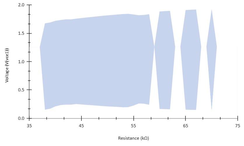
Figure 13. Area map highlighting upper and lower voltage range at vce1 between which chaotic behaviour was detected as a function of resistance at R in Mode 1.

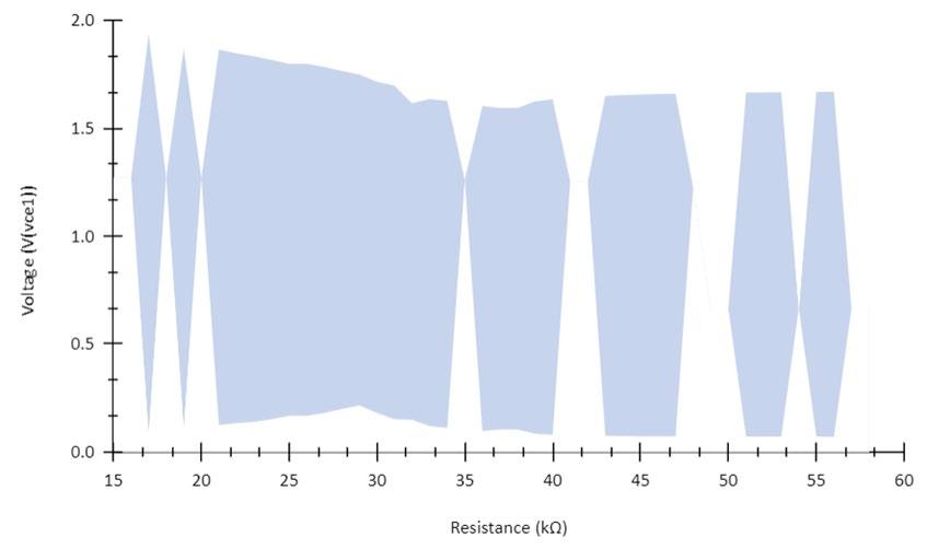
Figure 14. Area map highlighting upper and lower voltage range at vce1 between which chaotic behaviour was detected as a function of resistance at R in Mode 2.

Statistical Analysis:

The statistical test carried out utilised the procedure for the testing of chaotic dynamics by Bask & Gençay (1998). The Lyapunov exponents used were calculated using the TISEAN software (Hegger et al., 1999). The chaotic behaviour of the circuit in Mode 1 characterised by Lyapunov exponents in Table 1 show that there is a distinct range across which chaos occurs. The results found that chaotic behaviour (i.e. the range across which positive Lyapunov exponents were calculated) occurs between 39kΩ and 70kΩ. Similarly, the chaotic behaviour of the circuit in Mode 2 characterised by Lyapunov exponents in Table 2 shows that there is a less distinct range across which chaos occurs. The results found that chaotic behaviour occurs between 17kΩ and 55kΩ, however, there were significantly more and longer periods of non-chaotic behaviour within this range compared to Mode 1. These ranges of resistance are consistent with the graphs in Figure 11 and 12. All Lyapunov exponent values across all resistances in both modes were fairly small (with all λ < 1x10-1), indicating that observed chaotic behaviour in the circuit is weak. The magnitude of the Lyapunov exponents increased with increasing resistance (and thus an increase in chaotic behaviour) in Mode 1, whereas the inverse is true in Mode 2 as the magnitude of Lyapunov exponents decrease with increasing resistance (a weakening in chaotic behaviour)

Table 2. Summary of hypothesis test for Mode 1 of the circuit. α = 0.025. H0: λtest ≤ 0 vs. HA: λtest > 0. Mode 1

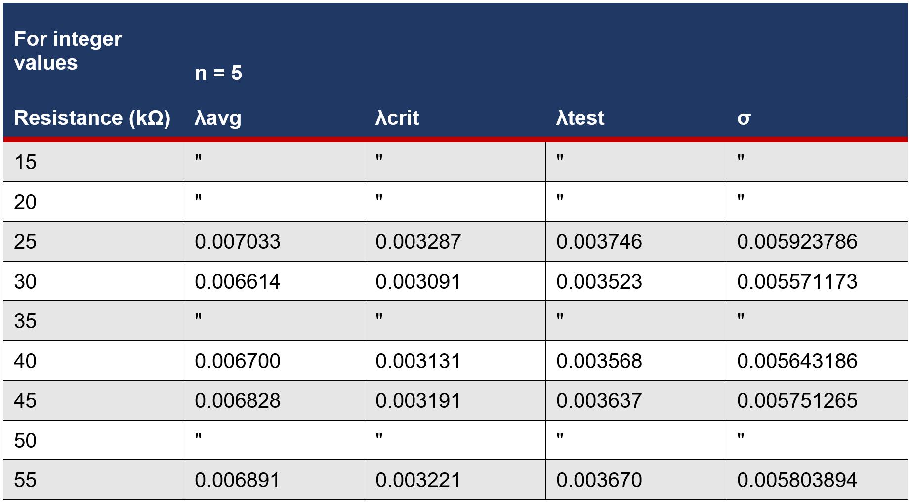
Table 3. Summary of hypothesis test for Mode 2 of the circuit. α = 0.025. H0: λtest ≤ 0 vs. HA: λtest > 0. Mode 2

Discussion

There exists a need for cheap and flexible simple chaotic circuits in fields such as robotics or encryption, (Tanougast, 2011), hence, this study has characterised the chaotic behaviour of the circuit proposed by Keuninckx et al. (2015) in two modes of the circuit. The findings of the study successfully demonstrate that chaotic behaviour occurs within both Mode 1 and Mode 2 of the circuit, both in-situ and insilico across a range of resistances, as positive Lyapunov exponents were obtained, therefore, the null hypothesis can be rejected, confirming the claims of chaotic behaviour by Keuninckx et al. (2015). The chaotic behaviour of the circuit was experimentally confirmed utilising an in-situ physical model of the circuit as expected oscillations in voltage, comparable to that of the LTSpice simulation of the circuit, were observed in both modes. Therefore, the further analysis done on using the simulated circuit is valid as it has been experimentally confirmed that chaotic behaviour does exist within the circuit.

Positive Lyapunov exponents (λ) were obtained across a range of resistances in both circuit modes, which is a strong indication of chaotic behaviour. This chaotic behaviour occurs in the circuit due to the feedback to the input from the components in the dashed box in Figure 2 (CHAOTIC CIRCUITS, n.d.) which creates a phase shift, inducing chaotic oscillations across the circuit. Interestingly, the range of resistances across which chaotic behaviour occurred in both modes was different as Mode 1 exhibited chaos from resistances between 39kΩ and 70kΩ, while Mode 2 from 17kΩ and 55kΩ, and the chaotic behaviour of Mode 2 was much more erratic and discontinuous with more and longer interspersed periods of periodic behaviour (λ < 0). This may bring into question the effectiveness of using Mode 2 in applications where consistent chaotic behaviour is needed, however, this interspersion of periodic behaviour may suit some applications where a both periodic and chaotic behaviour is needed. The values for the magnitude of the components (and the exact model of the transistor) used in this study differed slightly from the proposed components by Keuninckx et al. (2015), however, chaotic behaviour was still observed, indicating that this circuit design can be flexibly applied for a range of purposes in terms of cost and availability of the components Therefore, the chaotic circuit design characterised in this study is flexible and cheap (through utilising off-the-shelf components), providing the groundwork for future development of arrangements of similar circuit designs. This also increases the potential utility of such circuit designs in a wide variety of applications.

These findings of chaotic behaviour in the circuit are consistent with the findings of Keuninckx et al. (2015), who reported chaotic behaviour within Mode 1 circuit used, along with CHAOTIC CIRCUITS (n.d.) who also reported chaotic behaviour in this same circuit design. Chaotic behaviour in a circuit utilising relatively simplistic components is also consistent with the mathematical modelling by J. C. Sprott (2000) who found that chaos occurred in similar circuits.

The implications of a low-cost, flexible circuit made from off-the-shelf components are that it can be readily applied into physical applications at lowcost such as in image encryption or in robotics as the utilisation of chaos theory will greatly optimise and increase the efficiency of robotic functions and algorithms, especially when coupled with other technologies such as artificial intelligence or machine learning (Zang et al., 2016). This will allow for a new level of optimisation and productivity in these applications, such as in sensori-motor systems in complex robots (Steingrube et al., 2011), which could not be achieved with current, non-chaotic solutions. Moreover, the straightforward digital implementation of this circuit to create chaos could be useful not only for simulating certain patterns of chaos, but also for a range of software-based applications where chaos can be used to generate encryption keys or noise patterns.

Future research should be done into variations of this chaotic circuit design which utilise the resistor-capacitor feedback loop in order characterise a greater range of circuit designs using offthe-shelf components that display modes of chaotic behaviour. An improvement on the investigation could be through utilising greater quantifiers of chaos (such as fractals) as opposed to the simple maximal Lyapunov exponent calculation that was utilised using TISEAN software (Hegger et al., 1999). Hence, a possible direction for future research could be into quantifying the chaotic behaviour of this circuit (or circuits similar to it) across resistances on a micro-level utilising higher order chaotic quantifiers in order to observe the extent to which the circuit displays chaos.

Conclusion

This study confirmed the claim by Keuninckx et al. (2015) of chaotic behaviour in the proposed circuit in Mode 2, as well as Mode 1, by demonstrating that chaos occurs in both in-situ and insilico solutions. Through the use of data from the simulated circuit, positive Lyapunov exponents were obtained, rejecting the null hypothesis and indicating the range of resistances where chaotic behaviour occurs within the circuit. The circuit proposed is flexible and cheap, therefore, future research should be directed towards applying this flexible circuit into applications where the implementation of chaos greatly improves their efficiency and effectiveness, such as robotics and encryption.

Acknowledgements

I would like to thank Mr. Nicholson for his valuable guidance and feedback across all stages of developing, conducting, and finalising the report.

Reference List

Aristotle (1985) [OTH], On the Heavens,; in. J. Barnes (ed.), The Complete Works of Aristotle: The Revised Oxford Translation, Vol 1. Princeton: Princeton University Press. (n.d.).

Bask, M., & Gençay, R. (1998). Testing chaotic dynamics via Lyapunov exponents. Physica D: Nonlinear Phenomena, 114(1), 1–2. https://doi.org/10.1016/S01672789(97)00306-0

Bishop, R. (2017). Chaos. In E. N. Zalta (Ed.), The Stanford Encyclopedia of Philosophy (Spring 2017). Metaphysics Research Lab, Stanford University. https://plato.stanford.edu/archives/spr201 7/entries/chaos/CHAOTIC CIRCUITS. (n.d.). CHAOTIC CIRCUITS. Retrieved 4 December 2021, from https://www.chaotic-circuits.com/

Davies, B. (2018). Exploring Chaos: Theory And Experiment. CRC Press.

Guan, K. (n.d.). Important Notes on Lyapunov Exponents. 18.

Hegger, R., Kantz, H., & Schreiber, T. (1999). Practical implementation of nonlinear time series methods: The TISEAN package. Chaos: An Interdisciplinary Journal of Nonlinear Science, 9(2), 413–435. https://doi.org/10.1063/1.166424

Itoh, M. (2001). Synthesis of electronic circuits for simulating nonlinear dynamics. International Journal of Bifurcation and Chaos, 11. https://doi.org/10.1142/S0218127401002 341

Kajnjaps. (n.d.). Build a Chaos Generator in 5 Minutes! Instructables. Retrieved 5 November 2021, from https://www.instructables.com/A-SimpleChaos-Generator/

Kantz, H. (1994). A robust method to estimate the maximal Lyapunov exponent of a time series. Physics Letters A, 185(1), 77–87. https://doi.org/10.1016/03759601(94)90991-1

Keuninckx, L., Van der Sande, G., & Danckaert, J. (2014). A simple TwoTransistor Chaos Generator Based On A Resistor-Capacitor Phase Shift Oscillator. IEICE Proceedings Series, 46(C2L-A4).

Keuninckx, L., Van der Sande, G., & Danckaert, J. (2015). Simple TwoTransistor Single-Supply Resistor–Capacitor Chaotic Oscillator. IEEE Transactions on Circuits and Systems II: Express Briefs, 62(9), 891–895. https://doi.org/10.1109/TCSII.2015.24352

Khan, K., Mai, J., & Graham, T. L. (2015). Quantifying Some Simple Chaotic Models Using Lyapunov Exponents. 6(9), 4.

Lorenz, E. (1972). Predictability: Does the flap of a butterfly’s wing in Brazil set off a tornado in Texas? na.

Nazaré, T. E., Nepomuceno, E. G., Martins, S. A. M., & Butusov, D. N. (2020). A Note on the Reproducibility of Chaos Simulation. Entropy, 22(9), 953. https://doi.org/10.3390/e22090953

O’Connell, R. A. (n.d.). An Exploration of Chaos in Electrical Circuits. 43.

Oestreicher, C. (2007). A history of chaos theory. Dialogues in Clinical Neuroscience, 9(3), 279–289.

Petrzela, J., & Polak, L. (2019). Minimal Realizations of Autonomous Chaotic Oscillators Based on Trans-Immittance Filters. IEEE Access, 7, 17561–17577. https://doi.org/10.1109/ACCESS.2019.28 96656

Piper, J. R., & Sprott, J. C. (2010). Simple Autonomous Chaotic Circuits. IEEE Transactions on Circuits and Systems II: Express Briefs, 57(9), 730–734. https://doi.org/10.1109/TCSII.2010.20584

Rickles, D., Hawe, P., & Shiell, A. (2007). A simple guide to chaos and complexity. Journal of Epidemiology and Community Health, 61(11), 933–937. https://doi.org/10.1136/jech.2006.054254

Shaukat, S., Ali, A., Eleyan, A., Shah, S. A., & Ahmad, J. (2020). Chaos Theory and its Application: An Essential Framework for Image Encryption. 6.

Sprott, J. C. (1994). Some simple chaotic flows. Physical Review E, 50(2), R647.

Sprott, J. C. (2000). A new class of chaotic circuit. Physics Letters A, 266(1), 19–23. https://doi.org/10.1016/S03759601(00)00026-8

Steingrube, S., Timme, M., Woergoetter, F., & Manoonpong, P. (2011). Selforganized adaptation of a simple neural circuit enables complex robot behaviour. Nature Physics, 7(3), 265–270. https://doi.org/10.1038/nphys1860

Tama evi ius, A., Mykolaitis, G., Pyragas, V., & Pyragas, K. (2005). A simple chaotic oscillator for educational purposes. European Journal of Physics, 26(1), 61–63. https://doi.org/10.1088/01430807/26/1/007

Tanougast, C. (2011). Hardware Implementation of Chaos Based Cipher: Design of Embedded Systems for Security Applications. In L. Kocarev & S. Lian (Eds.), Chaos-Based Cryptography: Theory,Algorithms and Applications (pp. 297–330). Springer. https://doi.org/10.1007/978-3-642-205422_9

tseriesChaos: Analysis of Nonlinear Time Series version 0.1-13.1 from CRAN (n.d.). Retrieved 14 June 2022, from https://rdrr.io/cran/tseriesChaos/

vsiderskiy. (n.d.). Chua’s Chaos Circuit Instructables. Retrieved 5 November 2021, from https://www.instructables.com/ChaosCircuit/

Zang, X., Iqbal, S., Zhu, Y., Liu, X., & Zhao, J. (2016). Applications of Chaotic Dynamics in Robotics. International Journal of Advanced Robotic Systems, 13(2), 60. https://doi.org/10.5772/62796

Zeraoulia, E. (2011). Models and Applications of Chaos Theory in Modern Sciences. Science Publishers. https://doi.org/10.1201/b11408