THE TECHNIQUE OF DETERMINATION OF STRUCTURAL PARAMETERS FROM FORCED VIBRATION TESTING
TSANG, WAI FAN
http://hdl.handle.net/10026.1/2820
http://dx.doi.org/10.24382/3439
University of Plymouth
All content in PEARL is protected by copyright law. Author manuscripts are made available in accordance with publisher policies. Please cite only the published version using the details provided on the item record or document. In the absence of an open licence (e.g. Creative Commons), permissions for further reuse of content should be sought from the publisher or author.
PEARL https://pearl.plymouth.ac.uk 04 University of Plymouth Research Theses 01 Research Theses Main Collection 1994
University of Plymouth
THE TECHNIQUE OF DETERMINATION OF STRUCTURAL PARAMETERS
FROM FORCED VIBRATION TESTING
BY WAI FAN TSANG B.Sc. (Hons.)
A thesis submitted to the University of Plymouth in partial fulfilment for the degree of
DOCTOR OF PHILOSOPHY
SCHOOL OF CIVIL AND STRUCTURAL ENGINEERING
November 1994
i i

.......... -··. ..... ,. UNIVERSITY Of PL "MOUTH LIBRARY SERVICES Item Reo 222906 o No. Class T ( 1 o.g z -rsrr No. Contl. S""'S' No. I
ONLY
REFERENCE
THE TECHNIQUE OF DETERMINATION OF STRUCTURAL PARAMETERS FROM FORCED VIBRATION TESTING
Wai Fan Tsang
ABSTRACT
This thesis details the results of an investigation into a technique for determination of "useful" structural parameters from forced vibration testing. The implementation of this technique to full scale civil engineering structures was achieved by several developments in the experimental and computational fronts: a vibration generator and a computer-aided-testing system for the former and two computational algorithms for the latter.

The experimental developments are instrumental to exciting large structures and acquisition of large quantities of useful data in digital format. These data serve as inputs to the computational algorithms whose outputs are structural parameters. These parameters are in either modal or spatial forms which cannot be measured directly but have to be extracted from the raw data.
The modal-parameter-extraction method is based on direct Least-Square fitting technique and is simple to implement. The technique can yield good accuracy if the residual effects from out-of-range modes are removed from the raw data before fitting. The spatialparameter-extraction method distinguishes itself from other conventional methods in the way that the orthogona/ity property is not explicitly used. This method is applicable to situations where conventional methods are not; i.e. in cases if modal matrices are not square. Some success was achieved in cases in which computer synthesized or good quality laboratory test data were used.
Full scale field tests of a tall office block and a slender tower were carried out and their modal models obtained. Attempts to obtain spatial models of these structures were not carried out, however, as this task can be a separate research topic in its own right. Further research in such application is still required.
iii

Copyright Statement Title page Abstract List of Contents List of figures List of tables Nomenclature Acknowledgement Author's declaration I Introduction CONTENTS 1.0 Aims of this research 2 1.1 1.2 1.3 1.4 Background to this research An overview of the process of modelling Strategies and methodologies The scope of this research Forced vibration tests on civil engineering structures 2.0 Introduction 2.1 Review of previous works 2.1.1 Test methods 2.1. 1.1 Ambient excitation technique 2.1.1. I.l Wind 2.1.1. 1.2 Earthquake 2.1.1.2 Artificially induced excitation 2.1.1.2.1 Eccentric rotating mass (ERM) exciter 2.1.1.2.2 2.1.2 Historical Acco\lllt Rectilinear motion exciter 2.1.2.1 2.1.2.2 2.1.2.3 2.1.2.4 The pioneers in full scale testing The Earthquake Engineering Research Laboratory (USA) The Building Research Establishment (UK) Other investigations iv Page 11 Ul IV IX XVI XIX XXVUI XXIX 3 4 6 9 9 10 10 I I ]I 12 12 14 15 15 16 17 19
3 2.2 Contribution of previous works 2.2.1 Information feed back 2.2.2 Justification of the use of simple models 2.2.3 Empirical relationships 2.3 Limitation of previous works 2.3.1 Quantity of measurements 2.3.2 Quality of measurements 2.3.3 Test methods 2.4 Conclusions Theory 3.0 3.1 3.2 Introduction Concepts and approaches 3.1.1 Mathematical modelling 3.1.2 Structural modelling Theoretical approaches of modelling 3.2.1 3.2.2 Continuous systems 3.2.1.1 Formulation of problems 3.2.1.2 Methods of solution Discrete or Lumped systems 3.2.2.1 3.2.2.2 Formulation of problems Solutions using Finite Element Method 3.2.2.2.1 3.2.2.2.2 3.2.2.2.3 3.2.2.2.4 3.2.2.2.5 Construction of structural matrices Eigenvalue solutions Modes of Vibration Orthogonality of modes Application of Modal Analysis to 21 21 22 23 23 24 24 25 26 27 28 28 30 30 31 34 35 35 37 38 46 49 50 non-proportionally damped system 53 3.3 Experimental approaches of modelling 3.3.1 System identification 3.3.1.1 3.3.1.2 Black box approach Grey box approach 3.3.2 Implementation 3.3.2.1 3.3.2.2 Experimentation Frequency response function measurements V 59 60 61 61 62 62
3.3.2.3 Data analysis 65 3.3.2.3.1 Modal methods 65 3.3.2.3.2 Non-modal methods 66 3.4 Conclusions 68 4 Instrumentation 4.0 Introduction 70 4.1 The instrumentation system 70 4.2 The new excitation mechanism 72 4.2.1 Brief descriptions 73 4.2.2 Technical developments 75 4.2.3 Performance tests 77 4.2.4 Calibrations 80 4.3 Sensors and transducers 80 4.3.1 Stroke measurement 80 4.3.2 Accelerometers 81 4.3.2.1 Descriptions 81 4.3.2.2 Calibrations 81 4.4 Signal conditioning and processing 82 4.4.1 General signal conditioning 82 4.4.2 Signal recording 83 4.4.2.1 Analogue tape recording 83 4.4.2.2 Digital data recording 83 4.4.3 Excitation signal generation 83 4.4.3.1 Sinusoidal signals 83 4.4.3.2 Periodic random signals 84 4.4.4 Spectral analysis 84 4.5 Computer-Aided-Testing (CAT) 85 4.5.1 The hardware configuration 86 4.5.2 Control programs 87 4.6 Summary 88 5 Extraction of modal structural parameters from forced vibration data 5.0 Introduction 89 5.1 Conventional methods 91 5.1.1 SDOF-FIT methods 94 5.l.l.1 Circle-fit method 95 vi
5.1.1.2 Straight-line-fit method 97 5.1.2 MDOF-FIT methods 99 5.1.2.1 Partial fraction methods lOO 5.1.2.2 Gleeson's methods 101 5.1.2.3 Rational fraction Polynomial methods 101 5.1.2.4 Maia-Ewins's method 102 5.1.2.5 State space method 102 5.1.2.6 Frequency domain poly-reference method 103 5.1.3 Summary 104 5.2 The method used in this investigation 105 5.2.1 Backgro\Uld 105 5.2.2 Development of the algorithm 106 5.3 Implementation and Verification 114 5.4 Comparisons of the proposed with some conventional methods 125 5.5 Conclusions 128 6 Extraction of spatial structural parameters from forced vibration data 6.0 Introduction 129 6.1 Conventional modal methods 131 6.1.1 An overview of the Historical development 131 6.1.2 Methods requiring priori assumptions 133 6.1.3 Methods using ortbogonality properties 134 6.1.4 Methods using Optimization techniques 135 6.1.5 Summary of modal methods 136 6.2 The proposed non-modal method 137 6.2.1 Backgro\Uld 137 6.2.2 Development of the algorithm 139 6.2.3 Implementation and Verification of the algorithm 150 6.2.3.1 Computer simulations 150 6.2.3.2 Quality-of-fit factor 153 6.2.3.3 Results 155 6.2.4 Practical applications 160 6.3 Discussions 175 6.4 Conclusions 177 7 Full scale forced vibration tests on the British Rail (BR) building 7.0 Introduction 178 vii
8 9 7.1 Description of the structure 179 7.2 The test programme 181 7.2.1 Test environment 181 7.2.2 Test techniques 181 7.2.2.1 Ambient vibration tests 187 7.2.2.2 Steady state step-sine tests 188 7.2.2.3 Periodic random tests 190 7.3 Data recording and reductions 191 7.4 Test results 191 7.5 Analytical model of the BR building 206 7.6 Comparisons of experimental and analytical results 211 7.7 Summary 212 Full scale forced vibration tests on a fire drill tower 8.1 Introduction 213 8.2 Description of the structure 213 8.3 Test arrangements and procedures 214 8.4 Test results 216 8.5 Discussion of results 246 8.6 Summary 247 Conclusions and Recommendations 253 Appendices Listing of the CONTROL program Appendix 4.5.2 Appendix 5.3 Appendix 5.4 Listing of the modal parameter extraction program Comparison of errors in the modal parameters determined by the three methods Appendix 6.3 Appendix 8.3 References Listing of the spatial parameter extraction program A schedule of test identifications viii
LIST OF FIGURES
Figure 2.1.1.2-1
Figure 3.2.2.2-1
Figure 3.3.2.3.2-1
Figure 4.1-1
Figure 4. 2. 1-1
Figure 4.2.2-1
Figure 4.2.2-2
Figure 4.2.3-1
Figure 4.2.3-2
Figure 4.2.3-3
Figure 4.4.3.2-1
Figure 5.1.1.1-1
Figure 5.3-1
Figure 5.3-2
A photograph featuring the BRE's ERM exciter in the field
A simple bending beam subjected to shear and bending.
A schematic drawing showing the design, analysis, testing and redesign cycle
Schematic presentation of the configuration of the instrumentation system
A photograph showing the dismantled DARTEC hydraulic power system
A schematic drawing showing the hardware configuration of the excitation system. A photograph showing the excitation system. Acceleration responses of the loaded ram of the actuator over a range of input voltages and frequencies. Stroke responses of the loaded ram of the actuator over a range of input voltages and frequencies. Load generation capability of the exciter over a range of input voltages and frequencies.
The Hewlett Packard HP 3582A spectrum analyzer
A modal circle traced by consecutive FRF data points
Marking of resonant peaks with vertical lines on the modulus and imaginary lnertance FRF plots
Overlaid plots of original and regenerated Inertance FRF for the fictitious system with frequency resolution of 0.1 Hz and damping factor of 0.1 % of critical damping
Figure 5.3-3
Overlaid plots of original and regenerated Inertance FRF for the fictitious system with frequency resolution of 0.1 Hz and damping factor of 1 % of critical damping
Figure 5.3-4
Overlaid plots of original and regenerated Inertance FRF for the fictitious system with frequency resolution of I Hz and damping factor of 0.00 I % of critical damping
PAGE NUMBER 14
ix 38 67 72 74 75 76 78 78 79 84 96 121 121 I22 I22
Overlaid plots of original and regenerated Inertance FRF for the fictitious system with frequency resolution of I Hz and damping factor of 0.01 % of critical damping Overlaid plots of original and regenerated Inertance FRF for the fictitious system with frequency resolution of I Hz and damping factor of 0.1 % of critical damping Overlaid plots of original and regenerated Inertance FRF for the fictitious system with frequency resolution of 2.5 Hz and damping factor of 0.001 % of critical damping Overlaid plots of original and regenerated Inertance FRF for the fictitious system with frequency resolution of 2.5 Hz and damping factor of I 0 % of critical damping A schematic showing how the proposed method bypasses the conventional modal procedures to obtain the spatial matrices
Receptance spectrum for the 3 DOF fictitious system at spatial point No. I
Receptance spectrum for the 3 DOF fictitious system at spatial point No. 2
Receptance spectrum for the 3 DOF fictitious system at spatial point No. 3
Overlaid plots of original and regenerated Receptance spectra for spatial point I from a reduced model of order 6
Overlaid plots of original and regenerated Receptance spectra for spatial point 2 from a reduced model of order 6
Overlaid plots of original and regenerated Receptance spectra for spatial point 3 from a reduced model of order 6
Overlaid plots of original and regenerated Receptance spectra for spatial point 4
from a reduced model of order 6
Figure 5.3-5
Figure 5.3-6
Figure 5.3-7
Figure 5.3-8
Figure 6.2-1
Figure 6.2.3.3-1
Figure 6.2.3.3-2
Figure 6.2.3.3-3
Figure 6.2.3.3-4
Figure 6.2.3.3-5
Figure 6.2.3.3-6
Figure 6.2.3.3-7
Figure 6.2.4-1
the test set up and equipment used X 123 123 124 124 138 156 156 157 158 159 159 160 161
A schematic drawing showing
Figure 6.2.4-2 A schematic drawing of the four-mass torsional system 162 Figure 6.2.4-3 Correlation between the measured and the regenerated 162 FRF curves for the mass m 1 Figure 6.2.4-4 Correlation between the measured and the regenerated 163 FRF curves for the mass Figure 6.2.4-5 A schematic drawing showing the beam test arrangement 165 Figure 6.2.4-6a Overlaid plots of original and regenerated 171 to 6.2.4-6f Receptance FRF at all 6 spatial points on the beam (model A) Figure 6.2.4-7a Overlaid plots of original and regenerated 172 to 6.2.4-7f Receptance FRF at all 6 spatial points on the beam (model B) Figure 6.2.4-8a Overlaid plots of original and regenerated 173 to 6.2.4-8f Receptance FRF at all 6 spatial points on the beam (model C) Figure 6.2.4-9a Overlaid plots of original and regenerated 174 to 6.2.4-9f Receptance FRF at all 6 spatial points on the beam (model D) Figure 7.1-1 A photographic view of the BR Building. 179 Figure 7.1-2 A typical floor plan of the BR Building. 180 Figure 7.2.2-2 A time response record of the structure's amplitude response 183 Figure 7.2.2-3 Locations of the travelling and the reference 184 accelerometers in the BR building. Figure 7.2.2-4 Locations of the exciter in the BR building. 185 Figure 7.2.2-5a A photograph featuring the setting up of equipment 186 in the field Figure 7.2.2-5b A photograph featuring the fully assembled hydraulic 187 power supply unit in the field Figure 7.2.2.2-l A sample of typical time response recorded 189 Figure 7.2.2.2-2 A typical load spectrum when excitation frequency 190 was set at 1 Hz. Figure 7.2.2.2-3 The resulting acceleration response spectrum. 190 xi
Figure 7.4-1 a
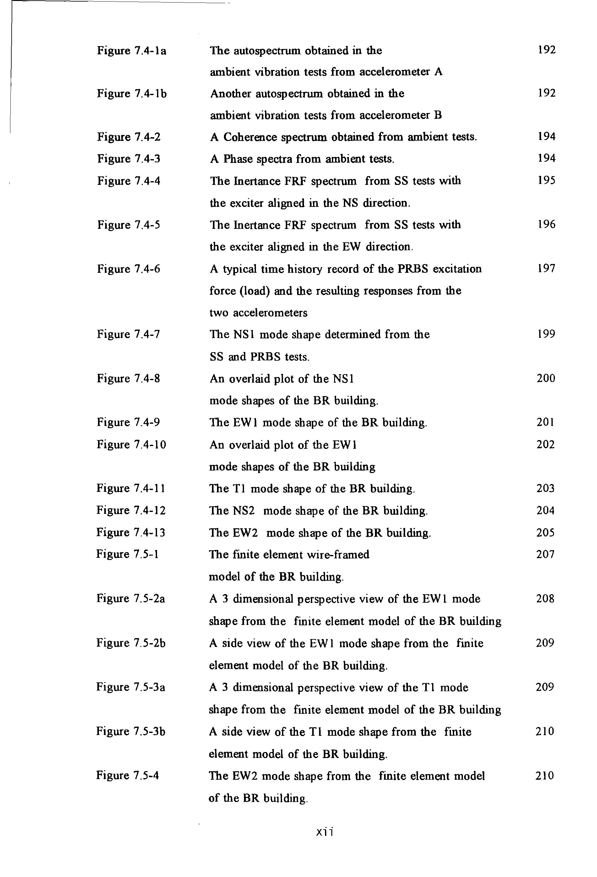
Figure 7.4-1 b
The autospectrum obtained in the ambient vibration tests from accelerometer A Another autospectrum obtained in the ambient vibration tests from accelerometer B
A Coherence spectrum obtained from ambient tests.
A Phase spectra from ambient tests.
The Inertance FRF spectrum from SS tests with the exciter aligned in the NS direction. The Inertance FRF spectrum from SS tests with the exciter aligned in the EW direction.
A typical time history record of the PRBS excitation force (load) and the resulting responses from the two accelerometers
The NS 1 mode shape determined from the SS and PRBS tests.
An overlaid plot of the NS 1 mode shapes of the BR building.
The EW 1 mode shape of the BR building.
An overlaid plot of the EW 1 mode shapes of the BR building
The T1 mode shape of the BR building. The NS2 mode shape of the BR building.
The EW2 mode shape of the BR building. The finite element wire-framed model of the BR building.
A 3 dimensional perspective view of the EW 1 mode shape from the finite element model of the BR building
A side view of the EW l mode shape from the finite element model of the BR building.
A 3 dimensional perspective view of the T1 mode shape from the finite element model of the BR building
A side view of the Tl mode shape from the frnite element model of the BR building.
Figure 7.5-4
The EW2 mode shape from the finite element model of the BR building.
Figure 7.4-2 Figure 7.4-3
Figure 7.4-4
Figure 7.4-5
Figure 7.4-6 Figure 7.4-7
Figure 7.4-8
Figure 7.4-9
Figure 7.4-10
Figure 7.4-11
Figure 7.4-12
Figure 7.4-13
Figure 7.5-1
Figure 7.5-2a
Figure 7.5-2b
Figure 7.5-3a
Figure 7.5-Jb
xii 192 192 194 194 195 196 197 199 200 201 202 203 204 205 207 208 209 209 210 210
A photographic view of the Camel's Head fire drill tower.
Locations of the exciter and designation of the grid points
Modulus inertance FRF spectrum using SS tests
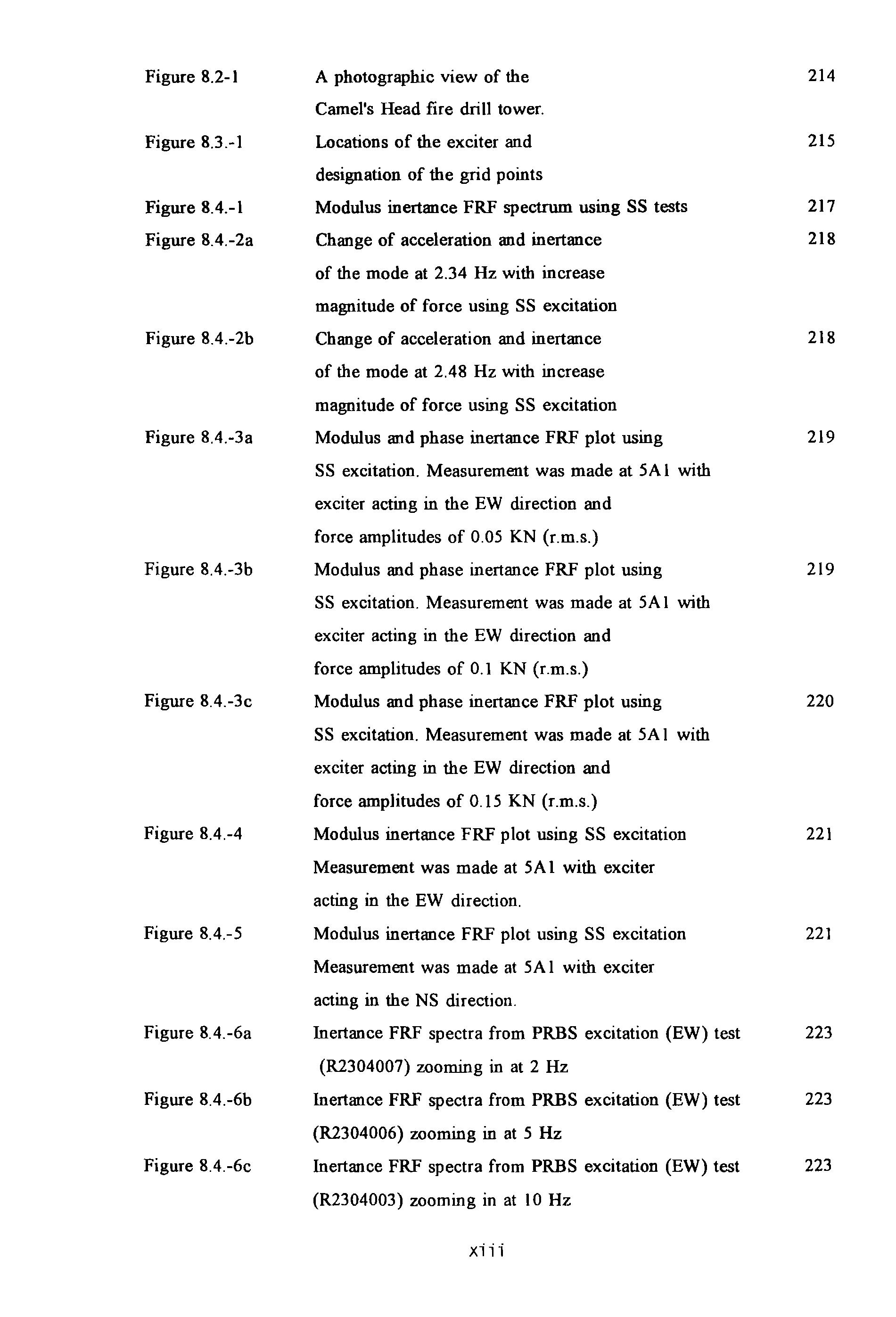
Change of acceleration and inertance of the mode at 2.34 Hz with increase magnitude of force using SS excitation
Change of acceleration and inertance of the mode at 2.48 Hz with increase magnitude of force using SS excitation
Modulus and phase inertance FRF plot using SS excitation. Measurement was made at 5A I with exciter acting in the EW direction and force amplitudes of 0.05 KN (r.m.s.)
Modulus and phase inertance FRF plot using SS excitation. Measurement was made at 5A I with exciter acting in the EW direction and force amplitudes of 0.1 KN (r.m.s.)
Modulus and phase inertance FRF plot using SS excitation. Measurement was made at 5A I with exciter acting in the EW direction and force amplitudes of 0.15 KN (r.m.s.)
Modulus inertance FRF plot using SS excitation
Measurement was made at 5A 1 with exciter acting in the EW direction.
Modulus inertance FRF plot using SS excitation
Measurement was made at 5A I with exciter acting in the NS direction.
Inertance FRF spectra from PRBS excitation (EW) test (R2304007) zooming in at 2 Hz
lnertance FRF spectra from PRBS excitation (EW) test (R2304006) zooming in at 5 Hz
Inertance FRF spectra from PRBS excitation (EW) test (R2304003) zooming in at 10Hz
Figure 8.2-1
Figure 8.3.-1
Figure 8.4.-1
Figure 8.4.-2a
Figure 8.4.-2b
Figure 8.4.-3a
Figure 8.4.-3b
Figure 8.4.-3c
Figure 8.4.-4
Figure 8.4.-5
Figure 8.4.-6a
Figure 8.4.-6b
Figure 8.4.-6c
xiii 214 215 217 218 218 219 219 220 221 221 223 223 223

Figure 8.4.-7a Inertance FRF spectra from PRBS excitation (NS) test 22S (R2S04001) zooming in at 2 Hz
8.4.-7b Inertance FRF spectra from PRBS excitation (NS) test 22S (R2S04002) zooming in at 5 Hz Figure 8.4.-7c Inertance FRF spectra from PRBS excitation (NS) test 226 (R2S04003) zooming in at 10Hz Figure 8.4.-7d Inertance FRF spectra from PRBS excitation (NS) test 226 (R2S04004) zooming in at 17Hz Figure 8.4.-7e Inertance FRF spectra from PRBS excitation (NS) test 226 (R2S04003) zooming in at 2S Hz Figure 8.4.-8a The modulus spectra obtained from the 228 grid point at SA 1 whilst the shaker was aligned along the EW direction Figure 8.4.-8b The phase spectra obtained from the 228 grid point at SA 1 whilst the shaker was aligned along the EW direction Figure 8.4.-9 Marking resonant mode positions at the peaks 229 in the modulus or imaginary Inertance spectra Figure 8.4.-10 Inertance FRF spectra from PRBS test (R2SX021X) 230 Figure 8.4.-11 Inertance FRF spectra from PRBS test (R2SY021 Y) 230 Figure 8.4.-12 Inertance FRF spectra from PRBS test (R2SY021 X) 23I Figure 8.4.-I3 Inertance FRF spectra from PRBS test (R2SY017Y) 231 Figure 8.4.-14 Inertance FRF spectra from PRBS test (R2SYOOIZ) 232 Figure 8.4.-ISa A view of the swaying EW I mode 234 Figure 8.4.-ISb Another view of the swaying EW I mode 234 Figure 8.4.-16a A view of the torsional Tl mode 23S Figure 8.4.-I6b Another view of the torsional Tl mode 23S Figure 8.4.-17 A view of the swaying EW2 mode 236 Figure 8.4.-I8a A view of the mode with natural frequency around 17 Hz 236 Figure 8.4.-18b Another view of the torsional T2 mode 237 Figure 8.4.-18c The mode with natural frequency around 18 Hz 238 Figure 8.4.-19 The mode with natural frequency around 24 Hz 238 Figure 8.4.-20 The swaying NSI mode 239 Figure 8.4.-2I The torsional Tl mode 240 xiv
Figure

Figure 8.4.-22 The NS2 mode 240 Figure 8.4.-23 The mode with natural frequency around 16 Hz 241 Figure 8.4.-24 The mode with natural frequency around 18 Hz 241 Figure 8.4.-25 The mode with natural frequency around 25 Hz 242 Figure 8.4.-26a The operating mode shapes at frequency 2.36, 10.2, to 8.4-26d 11.4 and 16.7 Hz with the exciter 244 acting along the EW direction Figure 8.4.-27a The operating mode shapes at frequency 2.36, 5.3, 10.2, to 8.4-27d 11.4 and 16.7 Hz with the exciter 245 acting along the NS direction XV
Table 4.3.2.2-1
Table 5.3-1
Table 5.3-2
Table 5.3-3
LIST OF TABLES
Comparison of the experimental and the manufacturer's calibration of the accelerometers
Table illustrating the mechanics of the calculation using the proposed algorithm
Assumed modal parameters for a four-modes fictitious system
Results of modal parameters determined using iterative mode subtraction for the four-modes fictitious system
Table 5.3-4
Table 5.4-1
Table 6.2.3 .1-1
Table 6.2.3.1-2
Table 6.2.3.1-3
Table 6.2.3.3-1
Table 6.2.3.3-2
Effects on QF Factors by using various mode combinations
Percentage errors in the modal parameters determined using author's method
Specified spatial parameters of the 3 DOF system used in the computer simulation studies
The specified mass matrix of the I 0 DOF system used in the computer simulation studies
The specified stiffness matrix of the I 0 DOF system used in the computer simulation studies
The reduced order 6 x 6 mass matrix of the l 0 DOF fictitious system determined by the algorithm
The reduced order 6 x 6 stiffness matrix of the l 0 DOF fictitious system determined by the algorithm
Table 6.2.4-l
Table 6.2.4-2
Table 6.2.4-3
Table 6.2.4-4
The derived spatial matrices of the torsional system (undamped model)
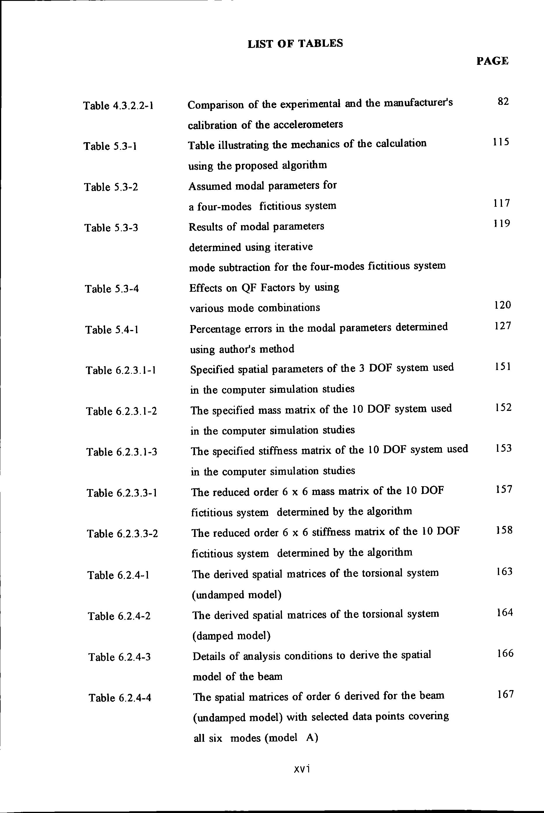
The derived spatial matrices of the torsional system (damped model)
Details of analysis conditions to derive the spatial model of the beam
The spatial matrices of order 6 derived for the beam (undamped model) with selected data points covering all six modes (model A)
xvi PAGE 82 115 117 119 120 127 151 152 153 157 158 163 164 166 167

Table 6.2.4-5 The spatial matrices of order 6 derived for the beam 168 (undamped model) with selected data points covering only four modes (model B) Table 6.2.4-6 The spatial matrices of order 6 derived for the beam 169 (undamped model) with selected data points covering only three modes (model C) Table 6.2.4-7 The spatial matrices of order 6 derived for the beam 170 (undamped model) with selected data points covering only two modes (model D) Table 6.3-1 The derived spatial matrices of the torsional system 175 (undamped model) using conventional modal approach. Table 7.4-1 The table of exemplary values of 198 the resonance frequencies of the various modes of the BR Building Table 7.6-1 The table of comaprison of the values of 211 the resonance frequencies of the various modes from experiments and the undamped natural frequencies from the finite element model Table 8.4-1 Zoom analysis with a resolution 224 of 0.04 Hz (EW excitation) Table 8.4-2 Zoom analysis with a resolution 227 of 0.04 Hz (NS excitation) Table 8.4-3 Modal parameters set determined from test data 220487001R (from 25 Hz PRBS tests with exciter 248 acting EW and measurements made at grid point 5A 1 in the EW direction) Table 8.4-4 Modal parameters set determined from test data 248 230487009R (from 25 Hz PRBS tests with exciter acting NS and measurements made at grid point 5 A 1 in the NS direction) Table 8.4-5 Modal parameters set determined from test data 249 2504870 17R (from 25 Hz PRBS tests with exciter acting NS and measurements made at grid point 5B2 in the NS direction) Table 8.4-6 Modal parameters set determined from test data 249 XVll
260487008R (from 25 Hz PRBS tests with exciter acting NS and measurements made at grid point 4A2 in the NS direction)
Modal parameters set determined from test data
R25X021X (from 25 Hz PRBS tests with exciter acting EW and measurements made at grid point 5A2 in the EW direction)
Modal parameters set determined from test data
R25Y023Y (from 25 Hz PRBS tests with exciter acting NS and measurements made at grid point 5B2 in the NS direction)
Modal parameters set determined from test data
R 25Y021X (from 25 Hz PRBS tests with exciter acting NS and measurements made at grid point 5A2 in the EW direction)
Modal parameters set determined from test data
R 25YO 17Y (from 25 Hz PRBS tests with exciter acting NS and measurements made at grid point 4A 1 in the NS direction)
Modal parameters set determined from test data
R 25Y001Z (from 25 Hz PRBS tests with exciter acting NS and measurements made at grid point OA 1 in the Vertical direction)
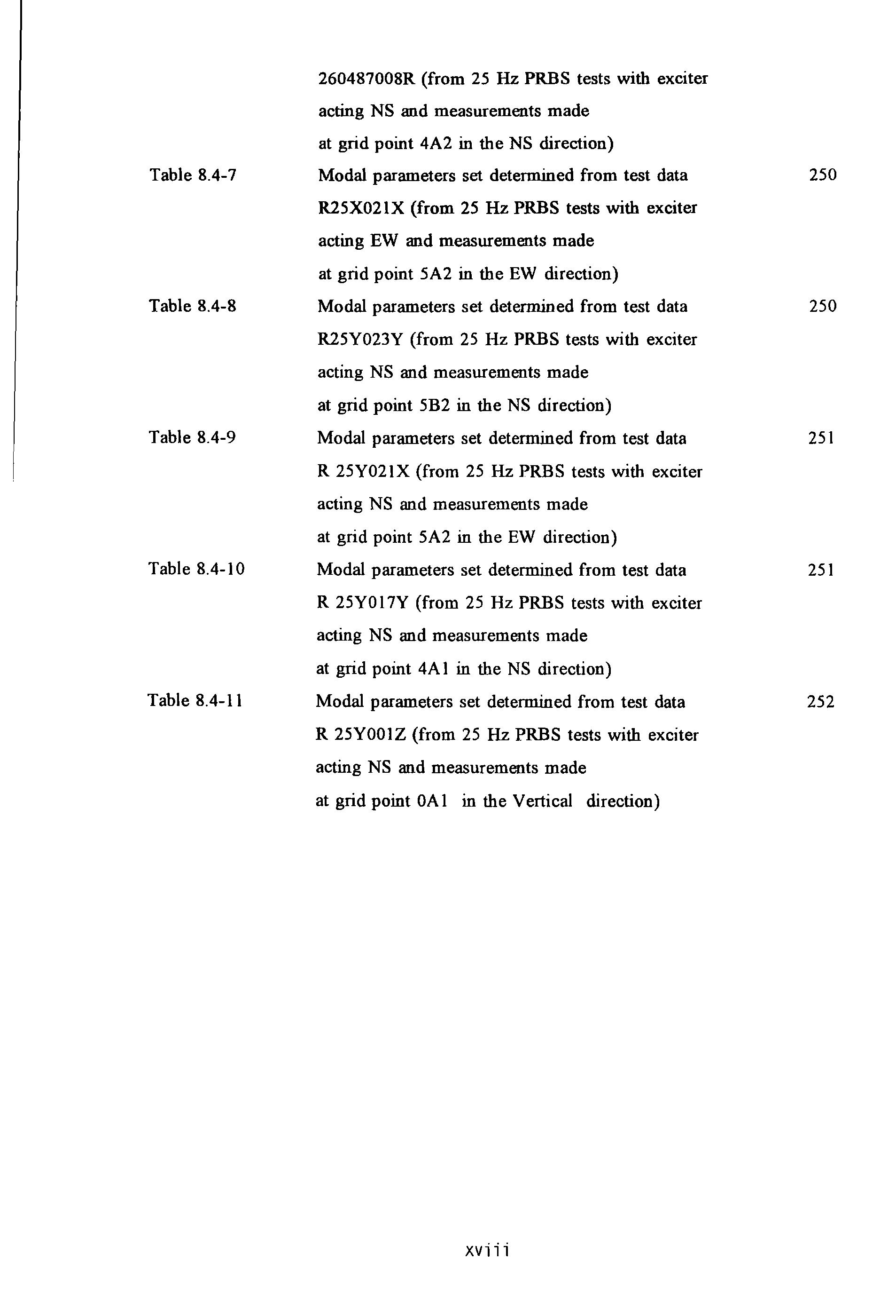 Table 8.4-7
Table 8.4-8
Table 8.4-9
Table 8.4-10
Table 8.4-11
Table 8.4-7
Table 8.4-8
Table 8.4-9
Table 8.4-10
Table 8.4-11
xviii 250 250 251 251 252
DEFINITION OF TERMS AND ABBREVIATIONS
Modal parameters
Computer-Aided-Testing
Finite Element Modelling
Boundary Element Modelling
Experimental Modal Analysis
Frequency Response Function
A set of parameters (natural frequencies, modal damping factors and modal constants) which characterise the modes of vibration of a physical structure
Spatial parameters
A set of parameters (mass, damping and stiffness)
which characterise the inertial, energy dissipation and elastic properties of a physical structure
Impulse Response Functions
Rectilinear motion hydraulic inertial exciter Eccentric rotating mass exciter
Step-sine excitation
Pseudo-Random-Binary-Sequence technique to generate random wave
Earthquake Engineering Research Laboratory in USA
California Institute of Technology, USA.
Building Research Establishment in UK
Earthquake Engineering Research Centre in USA
Central Electricity Generating Board
three dimensional xix
NOMENCLATURE
CAT FEM BEM EMA FRF
Chapter 1
IRF RMID ERM ss PRBS Chapter 2 EERL CIT BRE EERC CEGB 3D
Finite Element
wall ratio (the total length of all walls divided by the sum of the floor areas of all floors).
the natural frequency of vibration (in Hz)
natural period of vibration (in seconds)
number of storey of a building
height of a building width of a building
Engineering Science Data Unit
Degree of freedom
Strain and stress tensors respectively in indicia) notation spatial displacement vector in rectangular Cartesian coordinates
the internal body forces the surface traction
a function of differential operators
a fourth order elastic constants tensor the Young's modulus and Shear modulus respectively the two Lame constants mass density of material
dilatation
Laplacian operator
Finite Element Methods
Boundary Element Methods
a true solution of displacement u
a symbol denoting the domain an expression denoting the essential boundary conditions
an expression denoting the natural boundary conditions denoting the total boundary
a set of linear independent functions to approximate
FE r f ••• T N H B ESDU DOF Chapter 3 [ Eii ]and [crii] {u;} p E and G A. and 11 p A '\f2 FEM BEM n r. and rl Yk(x)
XX
a set of oodetermined parameters used to approximate Uo
residual error
a set of weighting fooctions
displacement in the y-direction along the length of the beam x arbitrary constants used to specify the deformation field of a beam
a polynomial matrix as a function of x used to specify the deformation fteld of a beam nodal displacements
strain energy
kinetic energy
Yooog's Modulus of a material

moment of inertia of a beam section axial and torsional displacement respectively
mass density of materials
angular frequency of vibration
Volume
length of a beam
mass matrix
stiffness matrix
damping matrix
displacement, velocity, acceleration vectors respectively in arbitrary Cartesian coordinates displacementt, velocity, acceleration vectors respectively in natural coordinates the modal matrix and is a matrix whose columns are eigenvectors is the transpose of modal matrix
are the diagonal Generalised mass, stiffness and damping matrices respectively are the rtb row stb column elements of the matrices [K*] and [M*] respectively
are the two proportional parameters used in the Rayleigh's damping model
£ 'I'; and w 11y or 11y(x) [POLY] u. S.E K.E. E I U,(x) and q(x) p V L [M) [K] [C) . .. {x}, {x}, {x} {1"]}, {il}, {i;} [ <I> ] [ <J> ]T [M*],[K*],[C*] K* and M* n n a and 13
xxi
the forcing vector is a diagonal matrix of modal damping factors is the spectral matrix and is a diagonal matrix of the eigenvalues ro,1 is the undamped natural frequency denotes the rlh mode when used in conjunction with modal parameters modal damping factor is eigenvectors (or natural mode shape) of the rlh mode is the diagonal matrix of modal damping factors are the amplitude and phase angle respectively used in defming the manifestation of a mode shape is a vector of phase angles c:p, the characteristic detenninant equals ro,( l - 1;1 , and is the damped natural frequency a damping matrix where the subscript nd denotes non-diagonal a damping matrix where the subscript re denotes it is a reconstruction a diagonal damping matrix which is obtained by retaining only the diagonal terms of the matrix [C.d] is a diagonal matrix constructed from known modal damping factors !;, and undamped natural frequencies ro, a proportional constant independent of frequency of harmonic oscillation used in describing energy dissipated by hysteretic damping is the amplitude of displacement oscillation is the frequency of harmonic oscillation is the viscous damping coefficient the coefficients of structural damping hysteretic damping matrix complex stiffness
a superscript denotes complex quantities are complex eigenvectors a complex modal matrix
{f} [I;] [ ro, 1 ] or [ro 2 ) ro, subscript r !;, <P, or {<)l,} [I; ] c, • Ql, { Ql, } A.d [C" ] [21;, ro, ] a c [yk] or [H)) ( l+ j y) [K]
xxii
denotes a complex conjugate of a vector
Single-Input-Single-Output
Single-Input-Multiple-Output
Multiple-Input-Single-Output
Multiple-Input -Multiple-Output
Frequency Response Function
receptance defined as a ratio of the spectral displacement response at coordinate i and the force applied at another coordinate j of a structure
Transfer Function
Discrete Fourier Transformation
denotes the Fourier Transform operator
Power Spectral Density function
a complex valued PSD function the Cross PSD functions of response x and force f the Auto PSD functions of force f and response x respectively a coherence spectral function
receptance defmed as a ratio of the spectral displacement response at coordinate i and the force applied at another coordinate j of a structure mobility defmed as a ratio of the spectral velocity response at coordinate i and the force applied at another coordinate j of a structure accelerance or inertance defmed as a ratio of the spectral acceleration response at coordinate i and the force applied at another coordinate j of a structure
{}* SISO SIMO MISO MIMO FRF or H(ro) TF DFT .'T( ) PSD G(ro) G,Jro) Grr(ro), G""(ro) COH,u,( ro) H,u(ro) or aij Hjro)
xxiii
Manufacturer of the hydraulic actuator
Manufacturer of the load cell used in calibration
Manufacturer of the accelerometers
Signal with constant amplitude and zero frequency
Frequency Modulation
Discrete Fourier Transform
Fast Fourier Transform
Analogue-to-digital converter
Time Domain methods
Frequency Domain methods is a hysteretic damping loss factor denotes the ilh mode of vibration when used in conjunction with modal parameters bysteretic damping matrix is the undamped natural frequency are the real and complex modal constants respectively magnitude of the complex modal constant is the total number of degree of freedom
(or modes) of the system denotes response at coordinate s and force at coordinate r
is the imaginary unit ./-1
single-degree-of-freedom multi-degree-of-freedom are quantities corresponding to any two neighbouring points (one on each side of the data point corresponds to ro; ) on a modal circle as shown in Figure 5 .1.1.1 -1.
SCHAEVITZ DC FM OFT FFT ADC Chapter 5 TD FD Y; subscript i [H] subscript sr J SDOF MDOF el , (J)I , e2 and (J)2
Chapter 4 DARTEC INSTRON
xxiv
is the diameter of a modal circle unknown parameters used in the rational fraction polynomial method receptance FRF and is a function of angular frequency ro ktb pole and its conjugate residue of the ktb pole and its conjugate damped natural frequencies (the imaginary part of a complex eigenvalue) damping coefficients (the real part of a complex eigenvalue) angular frequency are respectively the Fourier Transforms of displacement {x(t)} and force vectors {f(t)} and are functions of angular frequency ro.
undamped modal matrix
natural (or modal) coordinates is the diagonal modal or generalised mass matrix. is the diagonal modal or generalised stiffness matrix. is the diagonal modal or generalised damping matrix. the element of the stb row, itb column of the Wldamped modal matrix effective mass effective stiffness
effective damping is receptance (a complex quantity) and is a function of angular frequency ro reciprocal of receptance (or dynamic stiffness) the real and imaginary part of receptance respectively accelerance or inertance and is a function of angular frequency ro are the real and imaginary part of dynamic stiffness respectively
A'., (ro) and B'.,(ro) are the real and imaginary parts of the inverse of accelerance respectively
the modal damping factor of the ilh mode
n.ri H(ro) (J) {X} and {F} [ <I> ] 11 [M*] [K*] [C*] 41,j M.'· I K'. I C'. I a or a( ro ) 1/a 9'l and 3 y,.( ro ) A.,( ro) and B..( ro)
!;i
XXV
an indicial notation devised and defined to illustrated the mode subtraction operations where r is the mode number s is the number of iterative cycles performed quality-of-fit factor which quantifies the degree of correlation between two sets of data
Deriving Spatial Parameters from Experimental Data
US National Astronautical and Space Administration
Laplace Transformation operator
Laplace Transformation variable
Transfer Matrix
the real part of the vector {X( ro )}
the imaginary part of the vector {X( ro )}
the real part of the vector {F( ro ) }
the imaginary part of the vector {F( ro )}
the real part of a( ro )
the imaginary part of a( ro )
M(r,s) QF Chapter 6 DSPED NASA Sf() s [T) {XR( ro )} {XI( ro )} {FR( ro )} {FI( ro )} Ra( ro ) la( ro )
xxvi
the British Rail building
East West direction
North South direction
Root-Mean-Square
Name of a commercially available fmite element analysis software
Name of a powerful network computer manufactured by IBM
one-dimensional
root-mean-square
Test Identification used to encode different tests carried out attenuator dial reading
Motion Transmissibility
Name of a generally available graphics plotting software

Chapter 7 BR EW NS RMS PAFEC PRIME ID Chapter
r.m.s. TI %C MT GINO
8
xxvii
ACKNOWLEDGEMENT
The author would like to thank the University of Plymouth (formerly Plymouth Polytechnic) for providing financial support and the Science and Engineering Research Council for a grant (Grant No. GR/D/02119) which was instrumental in the purchase of the actuator. My next thanks go to my supervisors Dr. Clive Williams and Mr Peter Hewson (both Principal Lecturers of the University) for their foresight in the inception of the project.

I thank my past colleagues in the Polytechnic in general, those in the Department of Civil and Structural Engineering in particular. Special thanks go to Dr. Mike Foulkes (Lecturer) and Gregory Reagan (Research Assistant) who have helped in many ways.
Thanks also go to the teams in the University of Bristol and the Building Research Establishment for their invitation to join in as an observer when they carried out tests on the Humber Bridge and the Hume Point tower block in London.
TI1anks are also due to the British Rail and the Devon Fire Brigade for granting permission for me to carry out tests on the Plymouth British Rail Building and the Camel's Head Fire Station Tower respectively.
Thanks go to the Royal Naval Engineering College for allowing me to use college facilities during off-working hours for fmalizing this work. Thanks are due to past and present colleagues in the Department of Mechanics and Power with whom I have worked.
I would also like to thank my wife and my children for bearing a lot of the emotional aggravation and long periods of desertion which are, inevitably, part-and-parcel of research work.
Space limitation does not allow me to name each individual who helped in various ways, as I am sure the list would run to several pages.
xxviii
AUTHOR'S DECLARATION
At no time during the registration for the degree of Doctor of Philosophy has the author been registered for any other University award.
This study was financed with the aid of a position of research assistant from the former Plymouth Polytechnic and a grant from the Science and Engineering Research Council towards the equipment.
During this research, the author attended a course on Fundamentals of Structural Dynamics run by the Institute of Computational Mechanics, Southampton.
International Conferences and Seminars on Experimental Modal Analysis, Structural Dynamics, Identification and Smart Structures were attended at which work was often presented. Visits to laboratories of other institutions were made and discussions with other researchers undertaken.
Publications :
I. C Williams and W F Tsang. "Dynamic characteristics of reinforced concrete structures". Paper presented and published in the Proceedings of the Research Seminar on The Behaviour of Concrete Structures, Cement and Concrete Association, Fulmer Grange, 30 June - 2 July, 1986.
2. C Williams and W F Tsang. "Deterntination of structural parameters from full scale vibration tests". Paper presented and published in the Proceedings of the Conference On Civil Engineering Dynamics, University of Bristol, 24-25 March 1988.
3. W F Tsang, C Williams. "Application of Experimental Modal Analysis to full scale civil engineering structures". Paper presented and published in the Proceedings of the 3n1 International Conference On Recent Advances In Structural Dynamics, July 1988, University of Southampton, Paper 88.
XXIX
4. W F ·Tsang and E Rider. "Modelling of structures usmg experimental forced vibration data with a particular application in force prediction". Paper presented at the 4'h SAS-World Conference FEMCAD-88, Paris 17-19 October, 1988 and published 111 RNEC research report RNEC-RP-88023, Royal Naval Engineering College, Plymouth.
5. W F Tsang and E Rider. "The technique of extraction of structural parameters from experimental forced vibration data". Paper presented and published 111 the Proceedings of the 7'" lntemational Modal Analysis Conference, Las Vegas, 30 Jan- 2 Feb 1989.
6. W F Tsang , E Rider and P George. "Application of acceleration and strain measurements in forced vibration testing". Paper presented and published in the Proceedings of the Conference of Modem Practice In Stress And Vibration Analysis, University of Liverpool, 3-5 April 1989.
7. W F Tsang. "Use of dynamic strain measurements for the modelling of structures". Paper presented and published in the Proceedings of the 8'" lntemational Modal Analysis Conference, Orlando, Florida, 29 Jan- I Feb 1990.
8. W F Tsang, C Williams. "A comparison of some methods of modal parameters extraction". Paper presented and published in the Proceedings of the 8'h lntemational Modal Analysis Conference, Orlando, Florida, 29 Jan- I Feb 1990.
9. W F Tsang, R 1 Randal. "Identification of Rheological models of elasto-viscoplastic Electro-rheological Fluids". Paper presented and published in the Proceeding of the Intemational Symposium On Identification of Non linear Mechanical Systems from Dynamic Tests- EUROMECH 280. Ecully, France, 29-31 October 1991.
I 0. W F Tsang, R J Randal. "Use of Electro-rheological Fluids for Adaptive Vibration Isolation". Paper published in the Proceeding of the First European Conference On Smart Structures and Materials. Glasgow, UK, 12-14 May, 1992.

J. cr./.£ ..... . :XXX
Signed Date
CHAPTER 1 INTRODUCTION
1.0 AIMS OF THIS RESEARCH
The main aim of this research is to investigate the transfer of technology, developed in the so-called Experimental Modal Analysis field, to civil engineering applications: in particular, the technology of performing forced vibration testing to obtain useful structural parameters of full-scale civil engineering structures. The second aim is to improve or devise alternative testing methodology to the existing full-scale forced vibration testing methods adopted in civil engineering in the UK, by making use of an alternative excitation mechanism, a computer-aided-testing (CAT) system and computational algorithms to obtain the structural parameters.
1.1 BACKGROUND TO THIS RESEARCH
This research project was initiated in late 1984 as an extension of the work conducted by Williams JUJ in the mid 1970s. The objective of his work was to determine the real dynamic performance of some full scale civil engineering structures through in-situ vibration measurements. The initiative then, as it is now, was driven by the need for an experimental tool which could provide some information feed back for engineers to evaluate how a structure really behaved as a contrast to what was intended in the design.

Vibration can be a nuisance if it is not intended but can be very useful if it is skilfully induced to a structure. To most people, vibration is often perceived as something undesirable or as an early tell-tale sign of trouble in machinery. Perhaps this psychological effect can partly explain why most people show a negative feeling about vibration and very little tolerance to it in certain circumstances.
Excessive vibration not only causes physiological and psychological distress to the
inhabitants of a vibrating structure, it also causes structural 'distress' such as fatigue and failure of the materials of the structure itself. Hence, most engineers are taught how to avoid or eliminate vibration during their education. Very little emphasis is placed on the advantages of vibration.
Structural dynamicists have for many years, used controlled vibration as an interrogation tool in the same way as stethoscopes are used by doctors. This technology is branched into several subsidiaries. One branch is called dynamic testing which is widely used in the aircraft and automobile industries. As vibration tests can often be carried out non-intrusively and non-destructively, it is a very useful structural diagnostic tool.
Another branch is called condition monitoring which utilizes the detection of undue vibration as an indication of the 'health condition' or otherwise of machineries. Condition monitoring is widely practised in the field of power generation and propulsion industries involving high speed rotational machinery. Knowing the true state of health of machines means a saving of expenditure on unnecessary re-fits and early detection of faults can prevent an expensive repair bill because further and more serious damage can be avoided. Without this technique, actions taken are either too prudent or too complacent but both actions produce the same expensive outcome.
Traditionally, civil/structural engineers have little training on vibration. Unlike structural statics which is taught in all civil/structural engineering courses, structural dynamics is often reserved only for the specialists. Given this background, it is not difficult to imagine that a dynamic problem is often transformed to a quasi-static problem for design and analysis. In Britain, wind loading design is covered by the British Standard Code of Practice CP3 ll.ll.
Early civil engineering structures, especially those constructed in Telford's and Brunei's times, were less prone to ambient induced vibration. Structures built today are, however, increasingly lighter in weight, more slender in shape and more flexible as a result of the use of lighter but stronger construction materials. Such structures are more vulnerable to vibration from natural causes such as wind and/or seismic activities.
Misunderstanding of the effects of vibration can sometimes be fatal. The static behaviour of a structure cannot and must not be used to extrapolate to the dynamic

2
regime. A structure which is adequately designed for static loadings may not be adequate for dynamic loadings. The collapse of the Tacoma bridge was a typical example of such a tragedy. Critics often point their fingers at engineers for badly designed structures as the major promoter of misadventure. So a better understanding of the dynamics of structures is vital for the advancement of design and construction methods.
The following Sections introduce the theory and concept of forced vibration testing and explain how this technique can be applied.
1.2 AN OVERVIEW OF THE PROCESS OF MODELLING
Most investigative techniques, be they analytical or experimental in nature, can often be collectively described as modelling. Physical modelling which, often first springs to mind, is another modelling technique but is not of concern here. What is concerned here is mathematical modelling. Mathematical modelling is a prevalent task mutual to almost all analysis techniques. This exercise results in the realization of a complex system to a simplified conceptual model amenable to mathematical analysis.
Currently there are two mam approaches available in the field of structural dynamic modelling. One is theoretical, based on Finite Element Modelling (FEM) or Boundary Element Modelling (BEM) and the other is experimental, based on Experimental Modal Analysis (EMA ). FEM and BEM are instrumental in the modem practice of theoretical engineering analysis. However, recent advancement in instrumentation and signal processing technology is set to correct this imbalance. The dominance of analytical over experimental techniques is beginning to change.
FEM and BEM theories are based on a set of assumptions and idealizations upon which the feasibility and credibility of these methods depend entirely. The results of this analysis should never be accepted at their face values without the proper exercise of scrutiny. Otherwise, it is merely reduced to an unproductive "number crunching" exercise. Theoretical analysis alone cannot provide the sole solution to the need of a reliable engineering analysis tool. Other methods have to be sought to complement but not to substitute these theoretical techniques.
Experimental Modal Analysis which has been developing rapidly in another discipline,

3
is a very promising technique. The experimental technique advocated in this research is based partly on EMA (modal approach) and partly on another alternative called spatial approach. Modal approach relies on the determination of the modal parameters (undamped natural frequencies, modal damping factors and modal constants for each of the modes of vibration of a structure) to construct a modal model. Whereas spatial approach determines the spatial parameters (mass, damping and stiffness matrices) to construct a spatial model. The two approaches share some similarities in methodology but differ in the ways that data analysis or parameter extraction is carried out. Further explanation of these two methods will be given in chapters 3, 5 and 6 accordingly.

1.3 STRATEGIES AND METHODOLOGIES
The basic underlying methodology is called system identification and parameter estimation which originates from Control Engineering. In essence, system identification is a process of determining a mathematical relationship between the input and output of a system. Since its inception, its application to other disciplines such as Robotics, Aerospace and Mechanical Engineering has become increasingly popular. However, so far, Civil/Structural engineering is slow to exploit this technique.
In structural dynamics, characterization of a structural system is based on a set of simultaneous 'cause-effect' type measurements regarding the imposed forces (inputs) and the resulting responses (outputs) of a tested structure. This input-output relationship can be obtained in various forms such as Impulse Response Functions (IRF) or Frequency Response Functions (FRF). These two functions constitute a time-domain and a frequency-domain descriptions of a system respectively
IRF and FRF are regarded as secondary characteristics as they themselves are dependent on other more fundamental ones, called primary characteristics. Theory shows that the dynamics of a structural system can be characterised in terms of either a modal or a spatial model. In a modal model, the primary characteristics refer to the modal parameters (as defmed earlier). Modal theory stipulates that a structure's dynamics can be approximated by a scaled superposition of a sufficient number of vibration modes which are influential within the frequency band of analysis. Whereas in a spatial model, the primary characteristics refer to the spatial parameters (also defined earlier) which depict the inertial, elastic and energy dissipating properties of a system.
4
However, most of these parameters are 'latent' properties, usually not directly measurable quantities, and a computational algorithm is required to extract these parameters from the raw experimental FRF or IRF data. This extraction process is called parameter estimation. It enables a system's behaviour to be characterized based on only a handful of these parameters.
Having established a valid mathematical model, it enables either the imparted forces or the responses to be determined if the other one is known. Force detennination or response prediction are typical applications using this methodology.
Results and fmdings of a particular tested structure are more-or-less pertinent to that structure only and generalisation to other structures may not be allowed unless they are similar or identical in many respects. However civil engineering structures are rarely identical. Incurring research and development costs on a one-off product, rather than spreading them over millions of identical products such as cars, is often considered as uneconomical. A concerted and structured strategy is needed so that the individual test results can benefit the understanding of different forms of structures at large.
A so-called building block approach is fruitful to this end. Most structures are often built with simple and repetitive structural elements as building blocks. The understanding of the dynamics of these building blocks will help one to understand those of the structure as a whole.
The lack of understanding of some integral components of a structure has close bearing to some lapses in design philosophy and practice. Current practice often chooses to ignore the structural actions of the so-called non-structural elements believing that discounting their added strength is a prudent measure. With the cost of these elements often occupying a good proportion of the total construction costs, it make economic sense to find out if these discounted in-situ structural properties can be utilised in order to achieve optimum structural efficiency. In buildings, the structural actions of partition walls and exterior cladding have, for a long time, attracted strong interests. A number of investigations into the behaviour of cladding in tall buildings were undertaken by Oppenheim ll.Jl, Palsson ,._.., and Freeman IUI. But so far, the fmdings from these investigations are not comprehensive enough to warrant change in design practice.

5
Similar efforts were reported by a number of earlier investigators such as Honda 1u 1 , Blume and Binder 11 •71 in the early 1960s. They studied the changes in stiffness of a number of structures by measuring the corresponding changes in the global modal characteristics following different construction stages. This approach is obviously limited by the impracticality of performing tests within a hectic construction schedule. It is also difficult to obtain good quality data when disturbance of the sort expected to be found in a construction site is so prominent.
Computational methods were also undertaken such as an investigation carried out by Mirtaheri. IUJ This investigation was based primarily on numerical parametric studies. By performing numerous iterative computations, he attempted to construct some feasible analytical models which could be reconciled with measured modal characteristics. This approach, inevitably by its very nature, is largely a 'hit-and-miss' exercise and it does not always guarantee success. Again, alternative strategies and methods are still required.
1.4 THE SCOPE OF THIS RESEARCH
The scope of this research covers both experimental and theoretical work. The task was tackled by research and development in a number of key areas. These key areas covered vibration generation, measurement and analysis which were all considered to be essential to achieve the following stated objectives :

a. to develop an exciter which can excite large structures with random, sinusoidal or periodic forcing
b. to incorporate computer control in full-scale tests in the field
c. to develop algorithms which can extract useful information from forced vibration test data
d. to use the developed system/technique to determine the real characteristics and performance of a full scale structure
A special rectilinear motion hydraulic inertial (RMHI) exciter was developed for exciting large structure. This exciter was capable of generating excitation which conventional eccentric rotating mass (ERM) exciters could not do. According to the literature surveyed, the application of such an exciter to excite large structure was not well
6
documented. This research used this exciter on two civil engineering structures using both periodic random as well as step-sine (SS) excitation methods. The periodic random control signal is based on Pseudo-Random-Binary-Sequence (PRBS) technique. The two structures tested cover different types of building and structural systems: an eleven-storey reinforced concrete (RC) frame-shear-wall office building, and a slender RC frame tower used for fire fighting training.
In accordance with the stated objectives, a so-called computer-aided-testing (CAT) system was also developed. This system was formed by integrating a number of experimental facilities with a desk top computer which provided centralised automatic control of equipment and fast digital data processing and recording. With this system, the required test sequences could be pre-programmed and the correct setting of various testing instruments be 'switched' remotely and precisely by the computer under the control of a program. This system not only reduced testing time tremendously but also allowed better quality data to be obtained because the error-prone task of manual operation was alleviated. The CAT system was an essential and indispensable part of this research srnce the requirement of a large amount of useful data could not be satisfied without it .

Two computational algorithms were developed by the author during the course of this research. The first algorithm carried out the task of extracting modal parameters from measured forced vibration data. The method is similar to the dynamic stiffness method but is in direct least-square formulation. Although it is based on a single-mode assumption, with proper pre-treatment of data, this algorithm can yield good accuracy. A comparison of the algorithm and two conventional methods was also undertaken for comparison purpose.
The second algorithm extracts the spatial parameters which are a set of spatial matrices (mass, damping and stiffness matrices) which characterize an equivalent or 'reduced' structural model of a structure. The procedure is a "direct" approach which distinguishes itself in some ways from other conventional modal methods. The procedure was validated using computer synthesized as well as experimentally collected data. Promising results were obtained in most cases as the determined spatial matrices do provide a good model description of the tested structures especially simple ones ..
7
By following much the same principle, this research found that similar matrices can be derived using Strain Frequency Response data instead of Motion Frequency Response data. These matrices were also shown to be capable of providing a good model at least for the simple beam specimen tested. However, only the works using the "Motion" data are presented.
This investigation was intended to lay the ground work by solving much of the fundamental hardware and software requirements for full scale forced vibration tests. It was intended that the system developed could be used as a 'work-horse' for further investigations in the future. Results of the tests on the two structures are presented as test cases for the advocate technique.

8
CHAPTER 2 FORCED VIBRATIONS TESTS ON CIVIL ENGINEERING STRUCTURES
2.0 INTRODUCTION
This chapter is a review of some of the more notable works on forced vibration testing of full scale civil engineering structures. In general, these structures are usually so massive and complex that special considerations on excitation and measurement methods are required. Therefore methods applicable to tests in conventional laboratories are usually quite different from those used in the field on full scale ones. Although this review concerns civil engineering structures in general, buildings are emphasized more because a great number of tests were carried out on them.

This review begins with a summary of the test methods with a particular reference to the means of generating excitation. This 1s followed by a brief description of the fundamentals of the ambient and artificial means of excitation and a few examples of their applications. A more detailed historical account of the pioneering works on artificial forced vibration tests is also given. Finally, the various contributions and limitations of these works are discussed and conclusions drawn.
2.1 REVIEW OF PREVIOUS WORKS
This review 1s not intended as an exhaustive account of all previOus efforts but is only a highlight of those orthodox test techniques and procedures practised. In fact, a majority of these procedures is still being used today.
The literature study reveals that while forced vibration tests to other engineering structures
9
are reported quite extensively, only a few studies are concerned with full scale tests on civil engineering ones. The maJor impetus to the latter was attributed to only a few organisations notably : the Earthquake Engineering Research Laboratory (EERL) in the USA during the 50s and 60s, the Building Research Establishment (BRE) in the UK during the 70s and 80s and others in countries such as Japan and New Zealand .. Because of the strong influence from these organisations, the historical account of this development as detailed in Section 2.1.2 are naturally divided under these headings.

2.1.1 TEST METHODS
Before the invention of mechanical exciters, massive civil engmeenng structures could only be excited by natural means e.g. by winds and earthquakes. These means were by their very nature, not amenable to human control as regards to when and where they would occur. As a result, strictly limited information could only be obtained. Many artificial excitation methods were tried. From the one extreme where novelty methods such as explosives, gas turbine aero-engines and propulsion rockets to the other extreme where very primitive means were used. An interesting example could be found from a simple means of excitation using synchronized human body motion suggested by Hudson et al 12"1 ' 19641 back in 1964. It was primitive but nevertheless useful. So simple was this technique that its use was reported in other investigations. (Czarnecki tu. 19741 and Williams 11.1. 19791) Whatever the forms these various excitation methods might have taken, they served the same purpose i.e. to impart force/energy to a structure and set it into vibratory motion.
2.1.1.1 AMBIENT EXCITATION TECHNIQUE
Ambient excitation sources are those disturbances originated from the environment of a structure. For civil engineering structures, these disturbances are usually due to the ground, the hydro- and atmosphere: i.e. earthquake, wave and wind. Because these sources were uncontrollable, the quality of measurements obtained from these means was inferior to those from controlled excitation. However these methods offered a viable alternative in situations where expensive artificial excitation system were not available.
10
2.1.1.1.1 WIND
Wind was and still is one of the most commonly used technique in the field of civil engineering for exciting large scale building and bridge structures. The physics of wind is a complex subject and is beyond the scope of this short review to give a full description. In brief, wind is a result of the movement of atmospheric air due to difference in atmospheric pressure. The characteristics of wind is governed by the so-called short-term or long-term meteorological events. Apart from mean wind speed, another important physical characteristics is the temporal variation of wind speed called gust. The latter is particularly important for dynamic consideration and the former for quasi-static one.
In 1966, Ward and Crawford 12 4 • 1966 1 used this technique on a number of buildings. With some relatively simple equipment they demonstrated the feasibility of determining the dynamic characteristics of these buildings in this way. Since then, the interests m this technique grew and numerous researchers reported similar trials on a variety of structures : Trifunac 12'5' 19701 , Lam and Lam
2.1.1.1.2 EARTHQUAKE
Earthquake is a natural phenomenon which occurs as a result of the internal magmatic activities of the earth. However, small scale man-made earthquake can also be created for instance by underground nuclear explosion. Natural earthquake can occur with low to extremely high intensity which can produce catastrophic effects and cause damages and even destruction to structures.
As early as 1950s, Hudson 11'9' 19521 and Housner 12 ' 10 ' 19591 reported the use of explosives to generate ground motions. During 1960s, URS/ John A. Blume & Associates Engineers conducted an extensive structural response research programme which was sponsored by the US Energy Research And Development Administration. This programme lasted for more than I 0 years during which behaviours of a number of tall buildings resulting from nuclear underground explosions at the Nevada Test Site were monitored. In 1968, Jennings 11 11 • 1963 ; 1 ' 11 ' 19681 also reported a study on the response of yielding structures to earthquake excitation. His work improved the understanding of the failure and collapse modes of those structures due to strong ground motion.

1 2 6 • 19731 , Dalgliesh and Rainer 1 2 7 • 1978 1.
I I
In Japan, where seisiDJc activity is fairly active, similar investigations were also undertaken. One such work was reported by Hiroyoshi and Kobayashi '2 • 13 ' 19611 in 1960. However, very few publications were published in English and the extent of the works in this country cannot be ascertained.

1.1.1.2 ARTIFICIALLY INDUCED EXCITATION
Artificial excitation offers many desirable benefits over ambient ones. Indeed, the invention of artificial exciters added a new dimension to the ways vibration tests were carried out. With purpose-built, sophisticated exciters, controllable forces with sufficient magnitudes can be imparted to very big structures. The spectral characteristics of these forces can be tailored to the most meticulous requirements using modem electronics and signal processmg techniques. Artificial exciters have facilitated the development of many more powerful testing techniques. They came about in various shapes and forms: mechanical, hydraulic or electromagnetic etc. However, only works using the following two particular types of exciters are focused and discussed.
2.1.1.2.1 ECCENTRIC ROTATING MASS (ERM) EXCITER
The force generation mechanism m this type of exciter was based on utilizing the reactionary force due to the inertia from masses rotating at certain speeds. These masses were bolted to carriers at some eccentricity from the axis of rotation. Hence by varying masses and rotating speeds, forces of different amplitudes and frequencies were generated. With suitable arrangements of a number of these exciters, uni-directional harmonic forces or torques were produced. Such exciters are believed to have been first designed and built by Blume in 1934. These exciters were capable of producing 1.5 tonnes of force at about I Hz.
Later in 1961, Hudson tz.u, 1961 1 developed another one which, in many ways, was similar to the one built by Blurne but was different in the novel use of synchronization Synchronization of as many as four exciters was attempted. This system was able to generate a maximum force of 3.56 KN at I Hz.
Around the same period, another exciter was reported to have been developed in Japan by Takeuchi 12.Js, 19611 This was a 3-wheeled eccentric rotating mass exciter and was
12
capable of rotating at a maximum speed of 7 revolutions per second and generating 2.4 tonnes forces. Each wheel carried a mass of 20 Kg and a total mass of 60 Kg was required to produce this force.
Unfortunately, the attempts of synchronisation of a number of ERM exciters were unsuccessful because of the formidable problems in upholding the accuracy in speed control. Very accurate and stable speeds were required to provide a fme frequency resolution. It was not until significant improvements were achieved, by using modem electronics and control techniques, that the problem of accurate synchronization was solved. The improvements required were later adopted in the design of BRE's ERM exciters: a work undertaken by the University of Bristol. The prototype system was completed in December 1977 and the full system was operational by August 1978. A brief description of the few important characteristics of this system is given below.
The whole system comprised four separate exciters. Each one was driven by its own 'slave' control which were, in turn, under an overall control of a 'master' unit. This control was servo-driven which permitted a precision as fine as 0.001 Hz. Using crystal oscillator, the frequency of the control signals was maintained accurately to a precision of one part in 10 million. The maximum usable frequency of this exciter was about 20 Hz. The system produced harmonic forces, which were precise to within 3% of a maximum amplitude of around l tonne (at 1 Hz peak-to-peak). It also allowed each unit to be run either at 0 or 180 degree relative phase difference which was accurate to 0.01 radians. The exciters were mounted on heavy steel rings and designed as turnable to any desired orientation in the horizontal plane. Figures 2.1.1.2.1-l shows one such exciter mounted in the field.

13
2.1.1.2.2 RECTILINEAR MOTION EXCrTER
As a distinct contrast to ERM exciters, a rectilinear motion exciter operates in reciprocal and rectilinear motions . Hence it is able to generate a Wlidirectional force with just one Wlit. There is no need for delicate balancing as required in the case of ERM exciters Most rectilinear motion exciters belong to the electromagnetic, magnetostrictive or piezoelectric types However the drawbacks common to these exciters are very smaJJ force and stroke capacities and therefore are not app li cab l e to massive structures
Another type of rectilinear motion exciters is hydraulically operated and is branded as rectilinear motion hydraulic inertial (RMHI) exciters . As far as the author is aware, there is only a handful of literature reporting any attempt in the design, construction and application of such exciters . According to the literature s urveyed , one of the first of these attempts was reported to have been undertaken by Burrough et al 12 16 ' 19701 of the Central Electricity Generating Board , UK. in 1970 . Thi s exciter was reported as capable of generating a maximum of 11 tonnes force when operating at 0.46 Hz. This development marked a significant departure in the means of generating excitation force at low frequencies Another att empt was reported by Stephen, Hollings and Bouwkam p 12 17 ' 19731 in 1973 but th e outcome of thi s dev e lopment was not reported In

.·
Figures 2.1.1.2.1-1 A photograph featuring the BRE's ERM exciter mounted
14
1979, Galambos and Mayes 11.11• 19791 also reported using this type of exciter on an apartment block due to be demolished. However further details about this work was unable to be obtained.
2.1.2 A HISTORICAL ACCOUNT
A brief historical account of the developments in the early days in USA, UK, Japan and other places is given.
2.1.2.1 THE PIONEERS
The subject of resonance of a complete structure was first noted by Omori 11.19' 19911 in 1901. Later in the 1930s, a programme to investigate buildings' dynamic response was commissioned by the U S Coast And Geodetic Survey Jl.lo, 19361 after a string of disastrous earthquakes in California which caused a lot of damage to buildings and people. As a consequence of this programme, In 1934 Blume designed and built the first ERM exciter and used it to characterize the periods of vibration of some 212 buildings.
Later in 1958, Hudson, 11 .2 1 • 19611 of EERL, developed this type of exciter further to produce a new system capable of synchronizing several exciters. Around the same time, there was a similar development in Japan. Between 1960 and 1965, Takeuchi 11.15, 19611 and Karapetian ll.l2. 196s1 tried out their own designed ERM exciters on a large number of buildings in Japan. One of their major achievements was the successful compilation of the experimental results to produce a set of very useful empirical formulae describing the relationships between certain building characteristics in relation to their natural frequencies. These empirical formulae are widely adopted in various building design codes in a number of countries. They are valued as a very simple but useful guide for the initial stages of building design. (further details on these formulae can be found in Section 2.2.3)
Literature on the subject during these periods are in general very patchy. However it is reasonable to believe that these people are the pioneers in the practice of artificially induced forced vibration tests on civil engineering structures. Hudson Jl.ll, 19 .w1 and more recently Jeary 11.24• 1981 1 have summarized these early developments.

15
Research at EERL was started as early as 1950s by a number of eminent and internationally renowned academics in the field of earthquake engineering : Hudson, Housner, Keightley and Caughey etc. EERL was based at the Dynamic laboratory, Disasters Research Centre, California Institute of Technology in USA. In addition to the role as a leading research establishment in this field, EERL also served as an information centre administrating the publication and distribution of research reports and earthquake accelerograms to the earthquake engineering communities.
A programme of research was initiated at EERL under the sponsorship of the California State Division of Architecture and Constmction. This research was marked by the development of Hudson's ERM exciters in 1958. This work sta1ted a 'chain-of-reaction' later and as a result, a series of research programmes on buildings were carried out by various EERL researchers:

Nielsen used Hudson's exciters on two multi-storey buildings. Among his vanous achievements was the formulation of a series of equations from which the stiffness and damping matrices could be detennined using known information about the mass matrix and the experimentally determined modal properties of a tested structure. These equations were developed specifically for buildings which fitted the 'shear building' models and had infinitely rigid floors. He noted that because these equations were ill-conditioned, large errors often occurred in obtaining these matrices.
Jennings and Kuroiwa 12 32 • 1968 1 used the EERL's exciters on a library building with an objective to study the damping characteristics of this building. From the field measurements taken from this building, he discovered that the energy dissipation characteristics (measured as damping factors) of this structure tended to vary markedly with the amplitude of vibration and its loading history. The damping factors were found to vary somewhere between 0.006 and 0.02 during small and large amplitude vibrations. Larger amplitude vibrations were indicative of the energy dissipation levels to be expected in really strong earthquake conditions. They undertook another research project on another building with an objective of characterizing the interactions of the motion of the structure with its surrounding soil. During the course of this study, they discovered that the
2.1.2.2 THE EARTHQUAKE
(USA)
ENGINEERING RESEARCH LABORATORY
Hudson· 1 2 25 • l96-ll Keightley et al, 1 2 26 • 1961 1 Keightley, 1 2 27 • 1963 1 Nielsen,I2.2S,I96-II Bouwkamp and Blohm, 12 29' 1966 1 Kuroiwa 1230 • 19671 and Jennings 1 2 31 • 1071 1.
16
building acted as a 'force amplifier' (i.e. a force transmissibility larger than unity). This capability of amplifying the forces produced by a small excitation equipment to bigger forces imparting on the surrounding soil was perceived as a novelty at the time. It was regarded as such because without this technique, equipments of much larger scale would be required to produce such magnitudes of force on the soil directly.
Over a period of forty years, their works covered tests on a range of structures : dams, buildings and bridges etc. Further details on their works can be found in the cited publications by the EERL or the Earthquake Engineering Research Centre (EERC). The latter was a new organisation set up jointly by EERL and the University of California, USA. The EERC now performs much of the previous roles of the EERL. Their recent research activities include forced vibration tests on a number of concrete dams as reported by : Oougb and Cbang ll.JJ, 19841 of EERC and HaD and Duron Jl.l4J

2.1.2.3 THE BUILDING RESEARCH ESTABLISHMENT (UK)
In the UK, a long-term research programme was also initiated in the 1970's by the Building Research Establishment. The BRE is a government owned research establishment under the auspice of the Department of Environment, and is responsible for promoting research on subjects appropriate to the building and construction industries. The programme of work during this period was conducted in collaboration with a number of other organisations. The thrust behind these developments was the needs to provide real information regarding the dynamics of civil engineering structures, especially tall buildings. As a result of these works, the BRE has carried out one of the most extensive full scale dynamic test programme on civil engineering structures in this country. The structures investigated ranged from tall buildings, bridges, chimneys off-shore platforms to dams. Both wind and artificial forced vibration test techniques were used. A short extract from this wide spectrum of works are briefly described below.
Tests on several large multi-flue chimneys were carried out by Jeary and Winney
J2.3s,tmJ and Jeary (2.36, 1974 1 in the early 1970s using wind excitation technique. This work was a collaboration between the BRE and the CEGB. The results from field measurements reinforced a view that dissipation of most of the vibrational energy in these structures was due to the fundamental bending mode and that the damping values for this mode were
17
within the range from 0.03 to 0.05. These results justified the usual assumption of a value of 0.06 for damping in the design of these structures. This is a good example to show how experimental fmdings interact with design practices.
A rockfill dam and a buttress dam were also tested by Severn et al 1:z.:s7,t 979 ; 2.38, 191 ' 1 in late 1970s using the BRE exciters. This work was a collaboration between BRE and the University of Bristol. Amongst other things, this work discovered that the resonance frequencies of these dams had reduced as water level rose and that the experimental results were m good agreement with those from the corresponding three dimensional (3D) Finite Element (FE) models. This is yet another example illustrating the value of testing for validating analytical models. The results also demonstrated that forced vibration tests using artificial excitation on massive structures such as dams was plausible. Such application was considered unthinkable before.

Later, more research on more buildings continued covering a wide variety of building types and heights. They ranged from a 177 m high concrete communication tower to a 21m high office block. The programme of works during this period was marked by the collaborative efforts between the BRE and other organisations and by the proliferation of this technology to a wider sphere. The various organizations which had a formal involvement in this work included the Centre Experimental de Recherches et d'Etudes du Batiment et des Trauvaux Publics (France), Plymouth Polytechnic (now University of Plymouth) (UK) and University of Sheffield {UK). The results concerning the dynamic swaying characteristics of these buildings were reported by Jeary and Sparks 1139' 19771, A short extract of these findings are reproduced below :
a. Buildings which possessed shear walls and cores on the whole were found to have better sway resistance than those of similar dimensions that did not.
b. Cladding and partitions added additional stiffness against swaying : a structural action not quantifiable in design but measurable from experiment.
c. Torsional movements in buildings were a significant component of building's response to wind in addition to swaying.
d. Asymmetry in the distribution of mass and stiffening elements could lead to severe coupling between modes and produced complicated mode shapes.
e. A well designed building possessing reasonable amounts of shear and
18
bending resistance would normally have a fundamental ·mode shape of a straight line. Any deficiency in shear resistance would have made a building to take up a shear deformation mode which, for a gtven mass distribution, would have a higher associated modal mass than a straight line mode.
f. The modal damping factors for reinforced concrete buildings were found to be less than 0.0 IS in the normal circumstances. By implication, those buildings possessing damping factors in excess of this level could be suspect of suffering damages or considered as inadequately designed.
Their more recent research efforts include testing the Humber suspension Bridge in Humberside and Hume Point (the sister block of the infamous Ronan Point tower block) in London. Full details of their works are obtainable from the BRE publications. In summary, the contributions by BRE and others during the early periods were instrumental in consolidating the state-of-the-art of full scale forced vibration tests on tall buildings. The ERM exciter provided a good 'work horse' and established the position of artificial forced vibration testing as a useful structural diagnostic tool.
2.1.2.4 OTHER INVESTIGATIONS
This section samples and summarises research efforts by other individuals not already described above. Significant contributions were due to those in Japan : Kawasumi et al
J1.4o, 1956 1, Hisada et al 1 1 41 ' 19561 and Takeuchi 11' 15 ' 19601 whose works mirrored closely those of the EERL during the 1950s. As their works have already been described in other sections of this report, it is not to be repeated here.

Englekirk and Matthiesen 11.41 , 19671 reported tests on an eight storey reinforced concrete building using mechanical exciters to determine both translational and torsional responses of this building. They used two ERM exciters to generate excitation torques by running the two exciters at 180 degree out of phase. By doing so, they could excite large torsional response allowing a more accurate measurement of the centre of torsion of this building. This work is noted as one of the earliest attempts to excite a structure with a torque .
Much concern m the earlier days was focused on the interaction between cladding and
19
the main frame structure and recognized that full scale dynamic testing could provide an answer. A number of attempts tried to determine the effects on stiffness of structures from these non-structural elements. Some of these attempts were based on a methodology of detecting changes in modal characteristics at different stages of construction. Blume and Binder 11.43, 19"1 used this method on a 15 storey high steel frame building. Honda 12M. 19761 followed a similar line of thinking and his tests on three buildings revealed that reduction of some 60 to 70% of the periods of vibration could result from the addition of partitions.
More recent efforts along this line were also noted. Palsson 1:us, 191111 reported an investigation on the influence of heavily contoured precast concrete cladding panels on the overall dynamic behaviour of a 25 storey building. The building was symmetrical in the two principal directions and was of shear core construction. This study was both experimental and analytical. Huang ll.461 reported tests on two buildings to determine the changes in behaviour at different levels of excitation. His investigation showed that floor slabs did not behave as rigid diaphragms as normally assumed and that base movements were found to be too significant to be ignored. Such an assumption are still widely taken in the usual analysis of this type of structures.
Oppenheim 1 :u 7 • 19711 carried out similar studies on several buildings including a 20 storey reinforced masonry apartment block. His work led to the discovery of a behaviour mechanism between lintels and reinforced masonry walls which most analysis did not anticipate.
In summary, all the investigations reviewed here provide useful but fragmented information on the real behaviours of a range of civil engineering structures. Very few of these discoveries or fmdings have filtered through to be incorporated accordingly in design practice. The method of carrying out tests at different stages of construction was not entirely feasible both on teclmical or practical grounds. All these lead to a common conclusion i.e. much research effort is still needed to circumvent difficulties in the practice of full scale forced vibration tests on civil engineering structures.

20
2.2.1 INFORMATION FEED BACK
To. date, a wealth of knowledge about the real dynamic behaviours of tall building structures has been obtained. These fmdings help to substantiate certain facts which cannot have otherwise been found. Such information is invaluable in providing feed back to civil/structural designers to appraise their design i.e. to evaluate the assumptions and suggestions provided in design literature rather than accepting them without question.

Various subject areas necessary for further research are also highlighted after these works. They include :
the behaviour of tall buildings at various amplitudes of vibration i.e. non-linearity, the interactions of structures and soils, the interactions of structural and non-structural elements and finally, the significance and effects of torsional responses of building structures.
These continue to be subjects of great interest in civil /structural engineering.
2.2.2 JUSTIFICATION OF THE USE OF SIMPLE MODELS
For tall building structures of slight structural and geometrical complexities, simple lumped mass model are deemed acceptable in providing a first approximations of the natural periods of these structures. A multistorey building structure, of the sway-frame or central-core type construction, can be modelled as a 'shear building'. In formulating such a model, the masses of each floor level are lumped together at the floor level and the inter-storey lateral stiffness lumped together as a shear beam between the floors. Such idealization is found to be appropriate and more economical than formulating a full FE model. This modelling approach is adopted in a British design guide published by the Engineering Science Data Unit (ESDU a commercial establishment which provides authoritative and validated design methods and data for design).
Recommendations are provided in the forms of design data sheets or computer software programs (see ESDU (us, u 9 , :uo1 ).
2.2 CONTRIBUTIONS OF PREVIOUS WORKS
21
2.2.3 EMPIRICAL RELATIONSHIPS
The results of these full-scale tests on building structures are compiled to obtain a set of empirical formulae using statistical analysis techniques. These empirical relationships provide a means of estimating the natural frequencies f.at (or natural periods, T which are the inverse of natural frequencies) and the levels of damping of a building structure by simply considering a building's architectural characteristics such as the type, height H, number of storeys N, width B.
Taniguchi (:Ut( proposed the formula to calculate the fundamental natural period T of translational vibration of a building:

T = N * ( 0.07 to 0.09 )
Takeuchi ll.UI derived similar formulae based on the tests results of some 60 buildings carried out in the 1960s. His formulae modified Taniguchi's formula by the inclusion of a new parameter r : the wall ratio of a building (the total length of all walls divided by the sum of the floor areas of all floors). It is noted that other characteristics of the walls such as thickness and the positions of the walls were not considered. His results indicated that most experimental data on T were bounded by the values calculated by the following two equations :
T= (4+H*(l-4r)}
50
and T= (4+H*(l-4r)} 80
Other empirical relationships were also derived to determine the natural period of higher modes, such as :
( T of the 2nd mode ) = 3 * ( T of fundmnelllDI mode )
More recently, Ellis l:Z.Sll has also derived similar empirical formulae based on the field test results of a total of 163 buildings. Again these formulae utilize the overall dimensional characteristics of buildings as inputs parameters: The formulae are expressed as:
22
the natural frequency of the lowest translational mode: !1141 46
the natural frequency of the next lowest orthogonal translational mode:
f. = 58 1141 H
the natural frequency of the lowest torsional mode:
Most of these formulae are accepted in various British, Japanese and American Building Design Regulations and Codes of Practice (1.53, 2"54' 2.5S(. Although large errors are likely to occur in using these formulae, the simplicity of calculation is still an invaluable asset. These formulae are particularly useful because they permit an early estimation of the fundamental natural frequencies of a building long before any structural details are known. Any potential problem in terms of structural vibration can be spotted as earlier as when the overall architectural or dimensional details are finalised.

Like natural frequencies, damping factors of a building structure can also be estimated using similar empirical relationships. For instance, ESDU 12 -' 61 compiled the results of damping measurements from full-scale tests on a range of concrete and steel buildings to produce a series of design monographs. Except for some unusual structures, the estimates are generally acceptable_
1.3 LIMITATIONS OF PREVIOUS WORKS
Due to the lack of sophisticated instrumentation and computer equipment in the past, the results obtained are still somewhat scant and inconclusive_
1.3.1 QUANTITY OF MEASUREMENTS
Most civil engineering structures are complex in terms of sizes and structural complexities. For these structures, a large number of Degrees of freedom (DOFs) (hence the quantities
H
72 H
23
of measurement) are necessary to produce better models. Most pieces of equipment used in these studies were bulky and slow to operate. For instance, a modest computer was a bulky cabinet in those days rather than a small lap-top of today. To bring a computer to the field was unimaginable. As a result, only a very limited amount of data could be obtained within a short time. To gain any benefit from modern system identification methods, more measurements are required.
2.3.2 QUALITY OF MEASUREMENTS

The primitive testing equipment and inefficient procedures produced inferior results as judged by today's technology standard. Most equipments used in those days were not only laborious to use but also very troublesome to calibrate and to set up. Often, measurement records were analog and not digital in form. As a result, data retrieval and transfer were difficult and inaccurate. The quality of these measurements was also generally undermined because the tested structures were situated in their natural and uncontrollable environment. Extraneous sources of disturbance due to wind, traffic and human activities could not be eliminated. Noisy, spurious and incoherent measurements caused formidable problems to these investigations and limited their potentials
2.3.3 TEST METHODS
Ambient excitation techniques lack the sophistication and controllability that artificial excitation techniques have. Furthermore, they do not allow the direct measurement of the excitation forces. Hence the causality relationship, in terms of both amplitudes and phases, between the excitations and the responses cannot be determined. Consequently, these shortcomings render the aforementioned methods inappropriate and incomplete within the context of system identification.
ERM exciters offer some improvements but because they can only generate harmonic forces of a fixed frequency at any one time, they are both laborious and very time intensive to use. In fact, man-power and time are often the most precious resources in any field. test programme. Therefore wide band random test techniques can have greater potentials in this respect.
24
2.4 CONCLUSIONS
In conclusion, this literature study has highlighted the difficulties and shortcomings of the traditional methods used and suggested certain areas in need of improvement. Learning from these experiences, the priority in this research must be to device new test and data analysis methods to circumvent some or all these difficulties.

25
CHAPTER 3 THEORY
3.0 INTRODUCTION
Although this project is civil engineering oriented, much of the theories are not nonnally found in civil engineering. So instead of going straight into the theories on experimental modal analysis (introduced in Section 1.2), for the benefits of the readers from the civil engineering background, this chapter is presented under the main theme of mathematical modelling. Under this theme, this research is identified as an experimental modelling approach as a contrast to a theoretical modelling approach such as fmite element method which most civil engineers are familiar with. The bulk of the theories concerning experimental modal or spatial analysis are saved for deliberation in much greater depth later in chapters 5 and 6.

Much of the background theories underpinning this research come mainly from vibration and control engineering. The two disciplines share a lot of common ground. In fact, the mathematical foundations governing systems in control and structural vibration are strikingly similar. Nevertheless, fonnulation of equations and terminology differs a great deal. This chapter is not meant to be an exhaustive account of these theories but only an introduction to the ideas described in the following chapters.
There is no shortage of literature which deals with these theories in great depth. Some literature deal with very fundamental mathematical concepts such as existence and uniqueness of solutions to a fonnulated vibration problem. Others deal with highly complicated theoretical issues such as non-linearity etc. However, few practical engineers would find these theories interesting to read. A simplified approach is therefore presented here.
26
The concept of mathematical modelling in a wider context is introduced first. The more specific application of modeUing to structural dynamics is then explained. It is considered convenient and conceptually important to describe the conventional theoretical methods under the two categories: continuous (Section 3.2.1) and discrete approaches (Section 3.2.2) applicable to distributive and lumped systems respectively.
The steps leading to the derivation of the governing system equations are described: partial differential equations in the case of a continuous system or a set of linear ordinary differential equations in the case of a lumped system. The methods of solution of these equations are also briefly discussed.
In particular, Eigenvalue solution (Section 3.2.2.2.2), interpretation of Modes of Vibration (Section 3.2.2.2.3) and Orthogonality properties between different modes of vibration (Section 3.2.2.2.4) are introduced in this Chapter. Because these are important theoretical issues which need to be explained and are necessary pre-requisites before deliberating further theories in Chapter 5 and 6. The coverage in these Sections is intended to explain the concept of modal decomposition which forms the whole basis of theoretical and experimental modal analysis. The theories dealing with real modes (associated with undamped or proportionally damped systems) and complex modes (associated with generally or nonproportionally damped systems) are explained in much greater depth in Section 3.2.2.2.5.
The theoretical basis of the experimental approach of modelling, upon which this project is based, is reviewed in Section 3.3. The concept of system identification is introduced in Section 3.3.1 followed by the implementation of this methodology as given in Section 3.3.2. Data measurement and analysis methods are briefly explained in Section 3.3.2.3. Modal methods which derive models in terms of a system's modal parameters are briefly explained in Section 3.3.2.3.1. Non-modal (or spatial) methods which derive models in terms of a system's spatial parameters are also briefly explained in Section 3.3.2.3.2.

3.1 CONCEPTS AND APPROACHES
In essence, the basis of the approach of this investigation can be summarised as an exercise of mathematical modelling. The term mathematical is important here because it distinguishes itself from physical modelling which is the one usually perceived. Physical
27
modelling is a technique based on the Law of Similitude. By studying a reduced scale replica of the original structure, results are then extrapolated to those of the full scale structure. However the latter is not a subject of concern within the scope of this investigation.

3.1.1 MATHEMATICAL MODELLING
Mathematical modelling IS a process m which a complex physical system IS conceptualized and simplified so that it can be expressed in mathematical terms i.e. a series of so called GoverninJ!. Equalions. These equations are equivalent statements of some Laws of Physics, such as the Law of Conservation of Energy and the Newtonian Laws of Motion etc to name a few which are commonly used in the field of mechanics. Having fonnulated the governing equations in an appropriate form, a closed-form analytical solution can often be sought in the case of a simple model or an approximated solution in the case of a complex model, using available analytical or numerical methods.
The derived mathematical representation IS called a model whose major function is to characterize and predict the behaviour of the system studied. A useful model should be one which can make correct prediction in some if not in all situations. Most physical systems in the 'real world' are often too complex for any one model to take into account every single conceivable aspect affecting the system. Important factors have to be correctly chosen and less significant ones be discarded. This process is called conceptual idea/i:::alion. The well established fundamental Laws of Physics which most models are built upon are themselves products of conceptual idealization of nature.
Because idealized assumptions are introduced, the subsequent established model can only be treated as an approximation rather than an exact representation. Mathematical modelling is an art which requires both skill and good judgement rather than sheer manipulations of arithmetic. In most situations, this is carried out iteratively until arriving at an optimal model. This is particularly true for unfamiliar systems whose behaviour is not well understood.
3.1.2 STRUCTURAL MODELLING
Within the scope of structural mechanics, mathematical modelling is an essential and an
28
integral process in analysing structural/mechanical systems: from modelling of behaviours of structural materials, of simple structural elements such as beams and plates to those of complex integral structures in various shapes and forms.
In structural dynamics, structural resonance phenomena can be modelled quite successfully using Eigenvalue theories. Briefly speaking, the natural frequencies and mode shapes of a structure are analogous to the eigenvalues and eigenvectors of the corresponding system equations formulated for the structure (Sections 3.2.2.2.2 will give more details on this). Because mathematical modelling can provide a far-reaching insight into the dynamic characteristics of a structure, even before the structure is built, it is a very useful design and analysis tool.
In essence, the formulated governing equations furnish a relationship between the state of the system (or state variables) and the system parameters. In fluid mechanics, these variables are kinematic quantities such as flow velocity; thermodynamic quantities such as pressure, temperature, enthalpy or entropy. In structural dynamics, the state variables are force (or stress), displacement and its derivatives (or strain/deformation) at a spatial point (or coordinate) of a structure.
The system parameters refer to those quantities, usually constants in the temporal (time) domain, which depend on the geometric, configurational and the constitutive properties of materials of a system. At the microscopic (or material) level, these parameters refer to the Young's modulus, Shear modulus or Lame constants in the case of homogeneous and isotropic structural materials. Whereas at the macroscopic (or structural) level, these parameters are the inertial, stiffness and damping characteristics of an integral structure. It is the method of determining structural parameters (at the structural level) which is the principal concern of this investigation.
Structural models can have varymg degrees of sophistication. In many cases, simple methods are more preferential to use (especially for initial design purposes) than sophisticated ones as the latter often require considerable computational efforts. With the advances of computer technology and methods, models derived from finite elements or boundary elements theories are becoming increasingly popular and sophisticated.
Apart from theoretical means, the advances of computer and instrumentation technology

29
also allow structural modelling to be pursued by experimental means as well.
3.2 THEORETICAL APPROACHES OF MODELLING
The various approaches are explained according to the logical division of continuous and lumped systems. It can be shown that the equations of motion for both systems can be derived using the same set of principles. Among these principles, the Principle of Virtual Work (for static equilibrium cases) can be applied. This principle states: If a system of forces is in equilibrium, the work done by the externally applied forces through virtual displacements (compatible with the constraints of the system) is zero. For dynamic cases, the Virtual Work Principle can be extended to cover dynamic equilibrium using D'Alembert's principle which states that the resultant force must be in equilibrium with the inertia force in a system. Using Variational principle such as the Hamilton's principle, which reduces the problems of dynamics to the investigation of a scalar integral that does not depend on the coordinates system used. The Equations of Motions are obtained from the condition rendering the value of the integral stationary and this is the basis of the Lagrange's Equation.

3.2.1 CONTINUOUS SYSTEMS
A continuous system (or a continuum) is an assemblage of an infinite number of infinitesimally sized particles. All structures, apart from molecular or atomic structures, are continua by nature. By applying the Principles of Equilibrium for each individual particle, the differential equations of motion can be obtained. Alternatively, by integrating these equations within the boundary and domain of a continuum, the integral equations of motion can be obtained. The solution of these differential and integral equations m turn describes the distribution and the gross effects of the state of a system respectively.
A complete theory can be obtained from the mathematical theory of elasticity of solid bodies in general, and elastodynamics in particular. These theories deal with the determination of the state of infinitesimal strain within a solid body which is being subjected to the actions of an equilibrating system of forces. The restriction of infinitesimal strain is important to ensure the validity of linearization of the governing equations to be given below. Nonlinear equations are known to be notorious for presenting
30
difficulties in numerical treatment. Once the equations are linearized, complete solutions can be obtained by superposition of simpler solutions. Other simplified theories based on elementary theory of engineering mechanics are, in fact, derivatives or special cases of these theories. An excellent historical account of the development of the theories of structural modelling is given by Love Jl.tJ
3.2.1.1 FORMULATION OF PROBLEMS

In 1827, Navier derived a set of general governing equations of vibration of elastic bodies based on infinitesimal strain (geo metrical compatibility) and stress (force equilibrium) analyses These equations are now widely known as the Navier Equations which are fundamental to almost all continuum mechanics analysis. Full coverage of this theory is prohibitively long, therefore readers should find the missing details in other standard text books on this subject such as the one written by Love Jl tJ
The state of strain and stress in the body of a material is usually repr esented b y tensor s eu and cru respectively (using indicial notation) as given below :
The spatial displacement of each particle of the continuum is represented by a vector {u} (or u; for i = 1, 2 , 3 according to the convention of indicial notation which denotes x 1
€21 €31 €32 €33 a 11 a 12 a 13 a 2 1 a22 a 23 a 31 a 32 a33 3 .2.1. 1-la 3 .2. 1.1 - lb
3 1
, , x3 or x, y, z m the rectangular Cartesian coordinates) and the vanous strain components can be determined by pure consideration of geometry of small deformation .
The stress and strain tensors are both symmetric,
There are stx independent stress and strain components which occupy the upper triangles of the respective tensors . The condition of the equilibrium of forces m an infinitesimal particle allows the derivation of the equilibrium equations.
where F; p
j , j + F; = P * u is the internal body forces is the surface traction
or these differential equations can be written in symbolic form as (a 1i ) - P = 0
(3 2 1.1-4a) (3 2 1.1-4b)
Where is a function of differential operators .
The equations depicted above hold generally regardless of the materials involved However, the relationship between stress and strain is a function of the properties of a material known as the constitutive relations . In mathematical terms, this means that the stress and strain tensors are linked together by fourth order elastic constants tensor cijkl :
1 €; j 2 * ( u ; 'j + u j ' i ) (3 2 1.1-2a) where (3 .2
1.1-2b)
.
(3.2 1.1-3)
a;
3 2
Each coefficient cijkl of this tensor is an elastic constant. For isotropic and homogenous materials, these coefficients are functions of only two independent material constants called the Lame constants It can also be shown that the usual material constants : the Young's modulus E and Shear modulus G , can be expressed in terms of the two Lame constants A. and ll · Using indicia] notation , this relationship can be written as :
2 1 1-6)
In the absence of internal body forces F; , the following Navier's equations can be obtained :
.2 . 1.1-7)
where p is mass density of material and A , Y' 2 are given in extenso :
A = au 1 at.
called the dilatation
+
called the Laplacian Operator
After some manipulations , these equations can be reduced to the well known Wave Equations which describe the propagation of dilatational and shear waves in solids or the vibratory motions in an elastic continuum . Detail discussions on this subject are given by Clark ll.JI _

A closed-form solution can only be obtained if the compatibility (or integrability) requirements are also satisfied in addition to the equilibrium and constitutive requirements .
This is because the condition of a stress distribution in equilibrium with the given imposed
(3
.2 . 1.1-5)
(3
+
{3
33
loads does not necessarily imp ly a compatible strain fiel d and VICe versa. The compatibility equations are given below:
Equation (3 2.1.1-7) formulates the problem entirely in terms of displacements u;. The true solution would also require u; to satisfy the prescribed boundary disp lacement condition as well However since the problem is posed entirely in terms of displacements, compatibility Equation {3 .2. 1.1 - 8) will be satisfied automatically.

3.2.1.2 METHODS OF SOLUTION
Having derived the partial differential governing equations, it remains to find a solution when traction and disp lacements on the boundary of a continuum are prescribed.
(3 .2.
(3 2 1 1-Sb) (3 .2.1.
2 (3 .2.1.1-Sd) 2 (3.2.1. 1-Se) 2 (3 .2. 1.1 - Sf)
1.1-Sa)
1-Sc)
34
Under suitable conditions, a unique closed-form solution depicting the stress and strain state of each particle can be determined .
There are a variety of methods available to solve these equations : series, singularities, difference, collocation and variational methods to name a few . However it is beyond the scope of this thesis to fully explain these methods. Further details can be found in Love 13"11 and Ricbards 13•41·
3.2.2 DISCRETE OR LUMPED SYSTEMS
A closed-form solution to the governing differential equations shown in Section 3 .2. 1 can be very difficult to obtain except for simple cases only An alternative approach can be applied using approximations This approach performs a conceptual subdivision of the continuous domain into discrete elements of simpler forms . This process 1s often known as discretization There are two different techniques available in this respect i e a domain discretization method typified by Finite Element Methods (FEM) and a boundary discretization method typified by Boundary Element Methods (BEM). In domain methods , the governing equations of the problem are approximated over the region by functions which fully , or partially, satisfy the boundary conditions However in boundary methods, approximating functions are used which satisfy the domain but not the boundary conditions Though BEM are claimed to have certain advantages over FEM in some ways , such as :
a. a smaller problem size in term of data storage and computation ,
b . more efficient in handling problems with an infinite domain or small surface to volume ratio and
c . quicker to converge to a solution etc,
FEM are more popular with many commercial software available such as PAFEC , NASTRAN and ANSYS etc In contrast, very few commercial BEM software are availabl e
3.2.2.1 FORMULATION OF PROBLEM
FEM and BEM can be derived from the Weighted Residual, Variational or Functional principles Furthermore, it can be shown that the Weighted-Residue theory can provide

35
a unified description of both methods (see Brebbia ) The Weighted-Residual methods are numerical procedures for approximating the true solution Uo of a set of differential equations of the form :
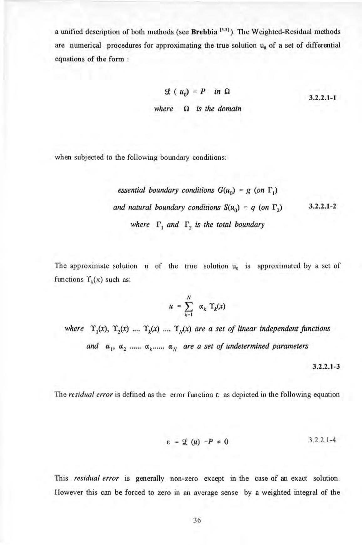
( uJ = P in 0 where 0 is the domain when subjected to the following boundary conditions :
essential boundary conditions G(uo) = g (on r 1) and natural boundary conditions S(uo) = q (on r :J where rl and r 2 is the total boundary
3.2.2.1-1
3.2.2.1-2
The approximate solution u of the true solution u0 I S approximated by a set of functi on s Yk(x) such as :
N
u = L at iix) A:=l
where i 1(x), i 2 (x) .... iix) .... iJ..x) are a set of linear independent fimctions and a l' a 2 at """ aN are a set of undetermined parameters
3.2.2.1-3
The residual error is defined as the error function t as depicted in the following equation e = (u) - P * 0
3 2.2. 1-4
This residual error is generally non-zero except in the case of an exact solution However thjs can be forced to zero in an average sense by a weighted integral of the
36
Convergence towards the exact solution is achieved as the number of terms increase. A variety of methods are available: the Galerkin's and the Rayleigh-Ritz methods to mention a few. However, a unified description of these methods can be obtained using the ideas of weighting functions w In its simplest description , the governing equation 3 2 2 1-1 can be re-written by the introduction of weighting functions :

where w is the weighting functions .
It can be shown that methods such as Galerkin's, Rayleigh's and Virtual Work only differ in the ways in which the weighting function s are cho s en . In the case of Galerkin's method , the weighting functions are chosen in the same way as the trial functions
Equation 3 .2 .2 . 1-8 produce a system of equations from which the unknown parameters ak can be solved
following form : J e '1' 1 dx = 0 for i = 1, 2,......... , N 3.2.2 1-5
'I'1 is a set of weighting junctions
where
J( (u) - P) * w * dO = 0 3.2.2.1-6
N J ( L at ik(x) ) - P) * 1'; * dQ = 0 k =l 3.2.2.1-7 where i = 1, 2, 3 ... ..... , N 3.2.2.1-8 where k= 1, 2, 3, ...... , N and i = 1, 2 , 3 ........ , N
37
3.2.2.2 SOLUTION USING FINITE ELEMENT METHODS
In essence, the analysis of an integral structure is broken down into one of an assemb lage of a large number of elements (called finite elements) which are of various shapes and sizes. Most structures can be idealized as an assemblage of b eams, membranes , plates etc. The results of discretization are manyfold. Firstly, a structure is replaced conceptually by elements forming a mesh : the lin es occur where element boundari es come together and the nodes where the element corners meet. Secondly , the governing equation s of the continuum are replaced by a set of simultaneous algebraic linear equations . Further theories on FEM can be found in some authoritative text books such as those written by Robinson 13 • 6 1 and Zienkiewicz 13 7 1
3.2.2.2.1 CONSTRUCTION OF STRUCTURAL MATRICES
The construction of the mass and stiffness matri ces of an integral structure is no different to assembling these matrices of the individual finite elements As an illustration , the con s truction of the structural matrices of a s impl e beam element i s shown. Figure
3 2 2 2 1-1 shows a beam bending in one of its principal planes Subjected to the usual assumption s as adopted in simpl e beam bending theories, th e displacement in the y-direction lly along the length of the beam x i s given by the following polynomial as a first approximation .

D D y L X
u uy 1 y 2
38
Figure 3.2 2 2 1-1 A simple bending beam with shear and bending moment at each node
where the a's are arbitrary constants. If expressed in matrix notation :
where {a} IS a vector of the constants a's and [POLY] is a polynomial matrix :

The constants a's can be solved if the nodal displacement boundary conditions are known . The choice of a 3'd order polynomial now becomes apparent since the four pieces of information on the nodal displacement enable the constants a 1, a3 and a4 to be solved . This relationship can be expressed in matrix form :
Therefore the displacement of any intermediate point between the nodal points can be interpolated using :
when expanded :
u = a + n.. x + a x 2 + a x 3 y 1 -.l 3 4 3.2.2.2.1-1
( u, I = [ POLY ] * ( a I 3.2.2.2.1-2
[ POLY ] = [ 1 x x 2 x 3 ) 3.2.2.2.1-3
{ ue } = [ A ] * { a } 3.2.2.2.1-4 where 1 0 0 0 0 1 0 0 3.2.2.2.1-5 [A ] = 1 L L L 0 1 2L 3L
{ uy } = [ POLY ] * [ A r• {ue } 3.2.2.2.1-6
3 2 2 2. 1-7 39
The strain energy S.E. associated with such beam deformation is given by : where
As by definition, the S .E. can also be expressed as :
In 3D analysis , a beam can be subjected to twist and axial deformations when under the action of couples and axial forces . As these deformations do not affect those due to flexure , the effects are combined together using superposition The axial and torsional displacements of any one point between the nodal points can be approximated by including the axial u,.(x) and torsional q(x) displacement fields :
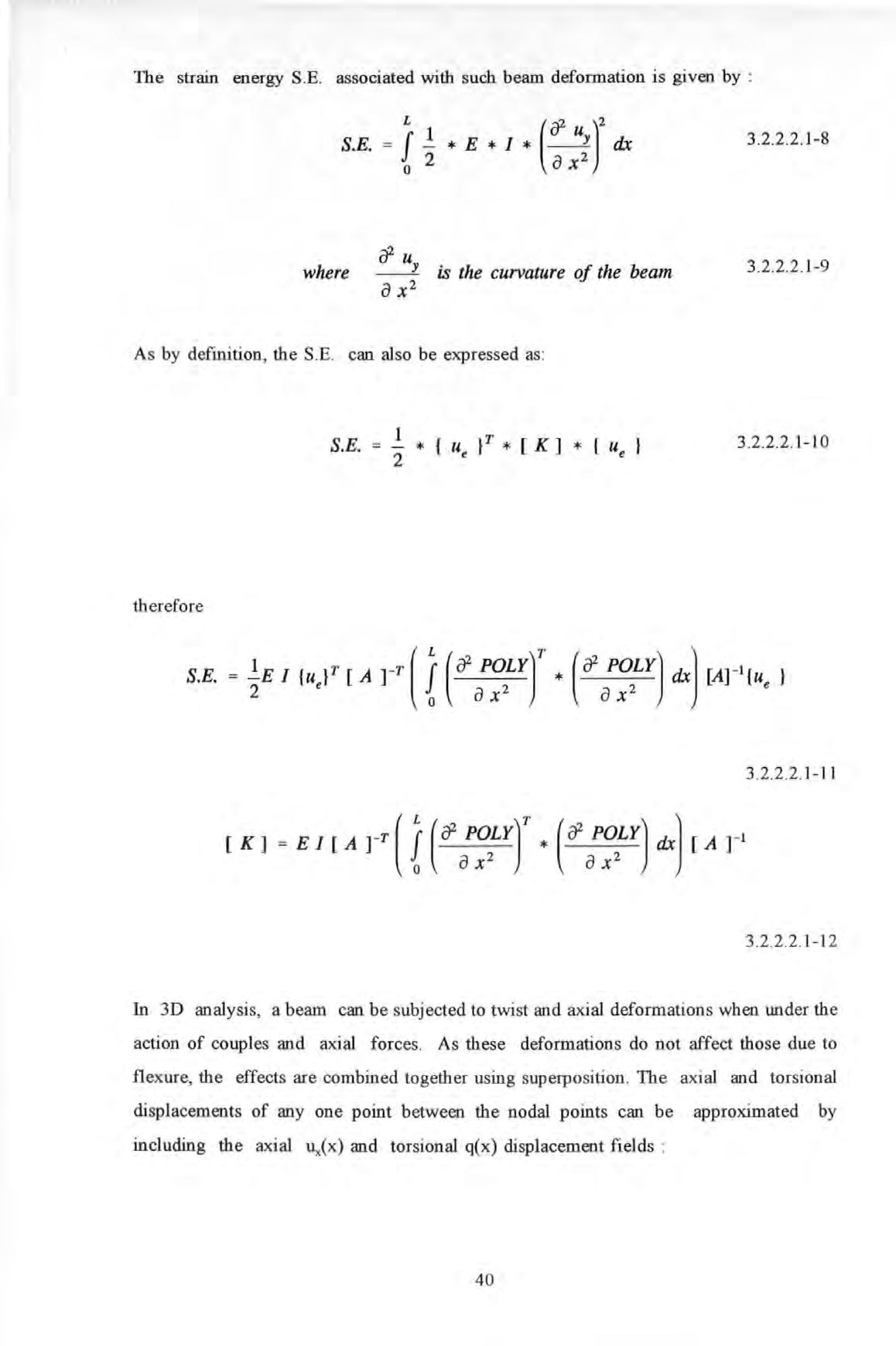
er uy a x 2
is the curvature of the beam
S.E. therefore 1 - -* { ut }T * [ K ] * { ut } 2 3.2.2 .2.1-8 3 .2 .2.2 . 1- 9 3 2 2 2 1-l 0 3 2.2 2 1-11 3 .2 .2 .2 . 1-1 2
40
Then the steps described previously can be repeated to determine the full stiffness matrix taking into account axial, bending, shear and torsion. This matrix is too large to be presented here and only the stiffness matrix due to shear and bending of a beam is given here:
Similarly , the mass matrix derived is based on Kinetic Energy considerations. The kinetic energy K.E of a beam with the aforementioned deformations is given by :
where ro is the angular frequency of oscillation
Also by definition, the K.E. can also be expressed as :
Therefore the mass matrix can be obtained by using :
Although the derivation process of a relatively simple beam element is shown , other elements such as membrane and plate bending elements etc. can also be obtained by
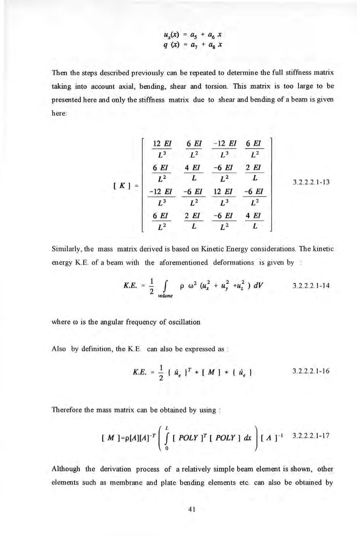
ux(x) = a 5 + a 6 x q (x) = a7 + a 8 x
12 El 6 El -12 El 6 El L3 L2 L3 L2 6 El 4 El -6 El 2EI L2 L L2 L 3 2.2 2 1-13 [ K] -12 El -6 El 12 El - 6 El L3 L2 L3 L2 6 El 2 El - 6 El 4 El L2 L L2 L
K.E. J volume 2 2 2 2 p w (ux + Uy +u4 ) dV
K.E. = .! { u }T * [ M ] * { ue 2 e
[M (! [POLY]' [POLY] dx) [A r' 3 .2.2 .2. 1-14 3 2 2 2 1-16 3 .2.2.2. 1-17
41
following these procedures :
a To make an assumption of the displacement fields which are appropriate to the element's geometry and proposed structural actions. These displacement fields are expressed in the form of polynomials and in terms of some arbitrary constants .
b To write the expression of the strain energy in terms of displacements by making use of interpolation to determine the displacements of any point within the element from the nodal displacements.
Having obtained the elemental structural matrices of each individual element, the global structural matrices can be obtained by assembling the individual elemental matrix. The end product of these operations is a set of linear algebraic equations ready for solution. So far, the theoretical development covers a free undamped system and these equations are usually stated as :

where {x} is a vector of nodal displacement
According to the coordinate system , the scheme of numbering of elements and nodes used , [M] and [K] are not usually diagonal matrices ([M] may be diagonal if lumped mass model is assumed) . In this case, the system of equations are coupled. Decoupling of the equations is achieved (to be proved later in Section 3 2.2.2 4) through linear transformation of the arbitrary coordinate system {x} to natural coordinates {ll} using the classical undamped modal matrix [<I>] (as illustrated in Equation 3.2.2.2 . 1-19):
3.2.2.2 . 1-1 9 (x} = [4>] *{ TJ}
Note that the coordinate transformation does not change the character of the system, it simply facilitates solution Pre-multiplying Equation 3 .2.2 2 .1 - 18 by [<I>]T and with the substitution of Equation 3.2 .2. 2 1-1 9, Equation 3 2.2 2.1-20 is obtained:
* ( ii } + [4>f[K]4>] * ( , } = ( 0 } 3 .2.2 .2. 1-20
Denoting :
[M) * { i } + [K] * ( x } ( 0 } 3 .2.2.2 1-18
42
[M*] and [K*] will be shown later in Section 3 2 2 2 3 that they are diagonal matrices and are usually called the Generalised mass and stiffness matrices respectively then a set of decoupled equations is obtained:
This technique of decoupling the system of equations forms the whole basis of modal analysis. The undamped modal matrix is obtained from the solution of an Eigenvalue problem which will be discussed in Section 3.2.2.2.2. The properties depicted in Equations
3 2 2.2 1-21a and 3 2.2 2 1-21b are termed orthogona/ity which is to be further explained in Section 3 .2.2 .2.3 .
The assumption of an undamped system is a mathematical convenience rather than a physical reality . Hence, the inclusion of damping in analysis is necessary . The analytical derivation of a damping matrix [C] is less trivial than those of [M] and [K] because, so far , there is still a lack of understanding of the mechanism and the means of modelling damping In fact , the subject of damping is a complicated subject in its own right. It is not the intention of this research to be indulged in the philosophical argument of what type of damping is really appropriate for the structures studied .
By definition , damping is a measure of the energy dissipating property of a material under cyclic loading conditions This energy is usually dissipated as heat or is absorbed by internal structural changes . The latter results in raising the energy level of a material or system. The three most popular damping mechanisms used are : viscous , hysteretic and Coulomb damping The different forms of damping all exhibit one feature in common : i e the cyclic load-deformation (or stress-strain) curve is not a single valued function but forms a hysteretic loop . The area enclosed by the loop represents the damping energy dissipated.

where [ f[M][ 11» ] [M*] 3 2 2 2 1-21a [ f[K][ ] = [K*] 3 .2.2.2 . 1-21b
[ M* ] * { } + [ K* ] * { 11 } = { 0 } 3.2.2.2. 1-22
43
Linear viscous damping prop erty is characterised by a dashpot Viscous damping force acts in a direction opposite to the direction of and with amplitude proportional to the amplitude of velocity of a coordinate. Viscous damping force is also frequency dependent. Hysteretic damping is associated with internal energy loss due to material hysteresis Hysteretic damping force acts in a direction opposite to the velocity of and with amplitude proportional to the amplitude of displacement of a coordinate. Coulomb damping is attributed from the energy loss by friction at an interface or joint between mating members where relative mechanical motion occurs Coulomb damping force acts in a direction opposite to the velocity of a coordinate and with constant amplitude It is independent of amp litud e of displacement and velocity of a coordinate. Both hysteretic and coulomb damping forces are frequency independent.
The choice of a suitable damping model is not usually an exact science and is often a matter of preference or convenience Viscous damping is widely used especial ly in the civil engineering community . However, some people show special preference to hysteretic damping because of the expedience it can offer in simplifying some complicated mathematical expressions.

In general, the decoupling technique using undamped modal matri x transformation does not work with any except a few very specialised forms of damping such as proportional damping :
Here, the damping matrix [C] is expressed as a linear combination of the mass [M] and stiffnes s [K] utili s in g two proportional parameters ex. and
This is often referred to as the Rayleigh's damping model. From Equation 3 2 2 2 1-23 , it can be observed that the damping matrix is also orthogonal with respect to the undamped modal matrix [<l>] sin.ce [M] and [K] both are and so as the s caled linear combination of them . A simple proof is now given . If Equation 3 .2 .2 .2 . 1- 23 is pre-multiplied and postmultiplied by [<I>t and [<l>] respectively , one can obtain :
[C] = a * [M] +P *[K] 3 .2 .2 .2 . 1-23
C = a * + p * [<Pf[ K ][<P] 3 2 2 2 1-24 44
Mter some appropriate substitutions, one can obtain :
where [C•] is a diagonal matrix similar to [M•] and [K.], and 1s called the Generalised Damping matrix
Hence the proof is completed From Equation 3 2.2 2.1-26 , one can obtain a relationship which enables the two Rayleigh' s constants a and J3 to be determined if values of modal damping factor and undamped natural frequency ro. are known

If experimental data on the modal damping factors is available, the damping matrix [C) can be constructed using (which is a diagonal matrix of the modal damping factors of the various modes of vibration), the analytically determined spectral matrix and the undamped modal matrix (i e they are obtained after solving an eigenvalue problem associated with the corresponding undamped system) :
is the undamped modal matrix
is the diagonal matrix of modal damping factors
is the diagonal spectral matrix
So with the inclusion of damping, the fully assembled equation of motion for a damped system under forced vibration is :
is the forcing vector
The stzes of the structural matrices [M], [C) and [K] depend on the number of degrees
3 2.2 2 1-25 [4lf = a [M•] + p [K1 = [C*]
+ 3 2 2 2 1-26
where I ( C ) = 2 ( rT ( ] ( W2 ] 2 ( 4l f [<I>]
[ro2 ]
3 .2 .2.2 .1-27
]
[M] * { x } + [C] * { .X } + [K] * { x } = { f } 3 2 2 2 1-28
{f}
where
45
of freedom required to specify the deformation fiel d. They can be very large even for a structure of modest size and complexity. Hence a process known as condensation (static or dynamic condensation) is often applied to reduce the size of these matrices before carrying out a computer solution. In essence, the original matrices are condensed by only retaining the master degrees of freedom and eliminating all the unwanted slave degrees offreedom in the equations It can be shown that in the case of static or dynamic condensation, the condensed stiffness matrix is exact, but the condensed mass matrix is not but an approximation only
A complete solution of the eigenvalue problem of large matrix size can involve very intensive computation However, if only a small number of the lower natural frequencies and mode shapes of a system is required , there are a few computational schemes available which do not require a complete solution

3.2.2.2.2 EIGENVALUE SOLUTIONS
Eigenval ue problems are found in many disciplines of science : buckling load analysis, principal stress-strain analysis etc to name a few in the field of structural mechanics So eigenvalues are not merely a set of mathematical quantities but are important physical characteristics of a system. The Eigenvalu e problem as found in structural dynamics are now deliberated Supposing a possible solution of the governing equations of a free undamped system (Equation 3 .2 .2.2.1-18) is of the form which is separable in timet and space:
Here {cl>,} is a shape function independent of time (it can be shown that this is actually a modal vector and subscript r denotes the rw mode of vibration of a system) and 11.Ct) is a time function By substituting Equation 3.2.2.2.2-1 to Equation 3 2.2 2 1-18 : 3 .2 .2.2.2-2
which is a set of N (the total number of degrees of freedom of a system) equations each of the type :
3 2 2.2 2-1
46
Using the method of separation of variables,
The positive sign is chosen for a conservative system. Hence two sets of equations are obtained :
The solution to Equation 3.2 2 2 2-5 is of the form :
where the amplitude c. and phase angle <p. are determined by the initial conditions. This solution stipulates that all the coordinates perform a harmonic motion with identical frequency ror and identical phase angle <p• The values of these frequency ro. are governed by the Equation 3 2.2.2.2-6 which can be recast in matrix form as:
which is the standard formulation for a special mathematical problem called Eigenva/ue problem A trivial solution to Equation 3 2.2.2 2-8 is {cilr} which is equal to a zero vector. Such a solution represents the static equilibrium case Non-trivial solutions exist if the characteristic equation (Equation 3.2 2 2 2-9) is satisfied
N N E mii lir<t>+ E ku 11r<t> = o for i=1,2,3 ........ ,N 3 .2 .2 .2.2-3 j•l j =l
N L kij ciljr J=l = constant (say N i=1,2,3........,N L mii ciljr j =l 3.2 2 2 2-4
lir(t) + w; TJr{t) = 0 N L (kii - (I); mii ) 4>1r = 0 for i=1,2,3 N j=l
1'1r
t + q>r) 3 .2 .2.2 .2-5 3 2 2.2.2-6 3 2 2 2 2-7
= er cos (wr
[K] * { 4>r } (I); * [M] * { 4>r } ( 3.2.2.2.2-Sa) or 2 = (l)r * { 4>r } ( 3.2.2.2.2-Sb)
47
where A cd is called the characteristic detenninant.
The solutions consist of a set of ro 2.'s (called eigenva lu es) and a corresponding set of {<jl,}'s (called eigenvectors) . Equation 3 .2 .2 .2 .2-8 is often expressed in full matrix representation as :
[ro,2 ] 1s called the spectral matrix and 1s a diagonal matrix of the eigenvalues ro, 2
m, is the undamped natural frequency
[<l>] is the real undamped modal matrix and is a matrix whose columns are eigenvectors (or natural mode shapes) of the undamped system's natural mode of vibration .
Since the [M] and [K ] matrices are both symmetric and positive definite , al l the eigenvalues ro, 2 will be real , positive numbers. Moreover, the eigenvectors of a symmetric matrix are in d ependent and the modal matrix [<l>] is non-singular Usually, all the eigenvalues are distinct but repeating values are possible for some systems When two eigenvalues are equal, the associated eigenvectors are ortbogonal to all the other eigenvectors but not orthogonal to each other: a characteristics known as degenerate However they can be taken in any linear combination to form ortbogonal eigenvectors The eigenvectors represent a unique shape but arbitrary amplitude (i.e values within any one eigenvector are relative and not absolute) These values can be fixed according to a process called nonna/isation. Hence the eigenvectors are called nonna/ mode shapes . There are a number of Eigenvalue solvers available : Jacobi , Householder, Cholesky and QR methods to mention a few
The theoretical development so far considers only an undamped system for which the eigenvalues m/ and eigenvectors {<!J,} are real However, for damped system with general forms of damping, the eigenvalues and eigenvectors will be comp lex quantities (i e complex modes) Later in Section 3 2 2 2 5, an entire Section will be devoted to cover the theoretical issues concerning genera lly d amped systems.

fled = I rKJ - w; [M] I = o 3 2 2 2.2 -9
where and [KJ * [ ] = [ w; ] * [M] * [ ] (3.2.2.2.2-] 0)
48
3.2.2.2.3 MODES OF VIBRATION
Each pair of eigenvalue and eigenvector is associated with a natural mode of vibration. The shape an undamped structure manifests when it is resonating in the rlh mode with frequency ro, is of the form :
where c, is a proportional constant and {q>, } is a vector of phase angles q>,

As mentioned earlier, the eigenvalues ro,2 and the eigenvectors {cl>} are real numbers for an undamped system . Hence the system possesses real normal modes. For a real mode, every coordinate of the system will oscillate synchronously and harmonically at a frequency which is the undamped natural frequency of that mode In other words , all coordinates reach their extreme displaced positions at the same time and the nodal (stationary) points remain the same over every cycle of oscillation The phase angles between coordinates (i .e . q>, ,) are either 0 or 180 degrees. The real modes are influenced by the system's mass and stiffness properties only
For a damped system, the deformation shape is of the form : where
ro,0 which equals ro,( 1 - )o.s is the damped natural frequency of the rth mode is the modal damping factor of the rlh mode
For a proportionally damped system, is non -zero , but the phase angles <p, , between coordinates are still either 0 or 180 degrees Hence, the system is oscillating with decayin g magnitudes (due to the exponential decay term), but the mode shapes are still real
For a generally or unproportionally damped system, eigenvalues and eigenvectors are complex numbers , hence the system possesses complex modes . A complex mode shape
3 2 2 2 3-1
{X} = Cr e - {,w,t {<J>r} COS (U>rD t + {cpr}) 3 .2 .2.2 .3 -2
49
exhibits a so-called 'galloping effect' i e. some coordinates will reach their extreme displaced positions some times after other coordinates reach theirs. This phenomenon is due to the difference in phase angles between them which are neither 0 nor 180 but somewhere between these two values .
3.2.2.2.4 ORTHOGONALITY OF MODES
In this Section, the mathematical basis of the important orthogonality property which exists between the different modes of vibration is given . The proof is conducted by considering any two modes of vibration : say modes rand s . As for mode r, the natural frequency and the modal vector for mode s should also satisfy Equation 3 .2.2.2.2-8 :

Since both [M] and [K] are symmetric matrices, then Equation 3.2.2.2.4-4 becomes :
Now let M",r and K"r• denotes the matrix triple products as depicted in Equations 3.2.2.2.47 and 3 2 2 2.4-8 (note the order of the matrix products is denoted by the subscripts : sr and rs respectively).
[K] * { 4>s } = w; * [M] * { 4>s } 3 .2.2.2. 4-1 By pre-multiplying Equation 3 2.2 2.2-8 and Equation 3 2.2.2.4-1 by {cp.}T and {cpr}T respectively to produce: 3 2 2.2.4-2 3 .2 .2.2.4-3 By transposing Equation 3 2 2 2.4-3 : 3 .2.2. 2.4-4
3.2.2 .2.4-5 So subtracting Equation 3 2.2 2.4-2 by Equation 3 2.2 2 4-5 : 2 2 7i ( Wr - W 3 ){ 4>s } [M] { 4>r } = 0 3 2 2.2.4-6
5 0
In general , all the natural frequencies of a structure are distinct i e. ror -:1:- ro , then
By following much of the above procedures once more, Equation 3 2 2 2.4-8 1s also obtained :

If ro r = ro , (i .e. for the sam e mode), then the matrix triple products are :
Hence K·r. and M•n are zero if r is not equal to s and are not zero if r is equal to s. In fact, K·r. and M·r. are the rth row sib column elements of the matrices [K•] and [M•] (the Generalised stiffness and mass matrices as introduced earlier) respectively Hence [K•] and [Mj are diagonal matrices The last four equations stipulate a property known as orthogonality (note that this statement is true only if [M] and [K] are symmetric matrices which are valid for most system s excep t nonlinear systems) The full matrix representation of the orthogonality properties involving all the modes are given as :
If the eigenvectors are nonna/ised in such a way as to make [M. ] an identity matrix , then the eigenvectors are called nonnal vectors or nonnal modes and matrix [Kj becomes a diagonal matrix known as spec tral matrix. [ro r/ l (or [ror2] as denoted earlier; subscript r is used instead of rr as the diagonality of the matrix is understood).
3 2 2 2.4-7
3.2 .2 .2.4-8
3 .2 .2.2.4-9 3 .2 .2 .2.4-1 0
[ <ll f[M][ <ll ] = [M •1 3 2 2.2.4-11 [ <ll f[.K][ <ll ] = [K *] 3 2 2 2.4- 12
[ (1) f[MJ[ <ll ] = [IJ 3 .2 .2.2 .4-13a 5 1
Recalling Equation 3 .2. 2 .2. 1- 20 :
Using the orthogonality properties , it can be simplified as:
Equation 3 .2 .2.2.4-14 represents a set of uncoupled second order differential equations wlllch are typical of the form (Note : the decoupling of equation of motions in the case of a damped system will be dealt with separately in Section 3.2.2 2 5 ) :
The solution to this equation is already given in Equation 3 .2 .2 .2 .2-7 . So any displacement {x} can be obtained by a weighted superposition of the harmonic motions (of all theN modes) with frequencies equal to the natural frequencies ro, , amplitudes c, and phase angles <p, as stipulated by the equation:
The philosophical importance of the property of orthogonality is that these orthogonal eigenvectors form a basis of the deformation space i .e. any deformation vector can be generated by a linear combination of these linearly independent eigenvecto rs . This statement is known as the expansion theorem which allows modal analysis to be used to obtain the response of a system from the knowledge of the system's modal properties
Orthogonality of modes are often used to check for the consistency of the experimentally measured modal vectors . These modal vectors should, in theory , be orthogonal to each other when weighted with respect to the mass , stiffness or certain limited form of dampin g matrices And as a common practice, the mass matrix is chosen in preference to the other two in testing the orthogonal condition because of the relative ease in determinin g masses

3 2 2 2.4-13b
; { 0 } 3 .2.2 .2 . 1-20
{ ii 1 + * { Tl } = { 0 } 3 .2 .2 .2.4- I 4
2 ii, + w, * Tl, 0 3 .2.2 .2.4-15
N {X} = [ {fl } ; L Cr {4>,} COS ((a), t + <p,) r=l 3.2 .2 .2.4-16
52
In general , the modal vectors obtained from experiments rarely satisfy Equation 3.2.2 .2.47 . This may be due to errors in measurement, in modal parameter extraction or in the assumed mass matrix. In practice, no alarm should be raised if Equation 3 .2.2.2.4-7 (using nonnal modal vectors) yields a value of not more than 0 1 (with normalisation, the modal mass of each mode has a value of unity)
3.2.2.2.5 APPLICATION OF MODAL ANALYSIS TO NON-PROPORTIONALLY DAMPED SYSTEM
So far, the modal analysis technique (i .e. the technique of decoupling the coupled equations of motion using undamped modal matrix transformation) as applied to undamped systems and systems with a specialised form of damping i.e proportional damping , has been discussed but not systems with the more general forms of damping. Proportional damping assumes that damping is a distributive property like mass and stiffness Such an assumption is not always justifiable especially in situations where heavy localised damping deyjces such as joint dampers , shock absorbers etc are applied to the system For nonproportionally damped systems, the damping matrix [C) cannot be reduced to a diagonal form by means of undamped modal matrix transformation :

i.e. [ <I> f * [ C ] * [ <I> ] is not a diagonal matrix
3 2 2 2 5-1
In these circumstances, there are a number of approximation schemes which, in essence, try to retain all the niceties associated with the proportionally damped cases One such scheme is applied in the following ways : let [Cnd] = [<l>f [C] [<I>]
3 2 2 2 5-2
i.e the original system damping matrix is pre- and post-multiplied by [<l>]T and [<I>] to obtain a matrix [Cod ] where the subscript nd denotes non-diagonal . Then a new system damping matrix [Cr ] (where the subscript re denotes reconstruction) is reconstructed by :
3 2.2.2 5-3
The matrix [Cd] is a diagonal matrix which is obtained by retaining only the diagonal terms
from design drawings .
53
of the matrix [Cnd1· Another scheme works very much the same way. The matrix [Cod] is reconstructed based on Equation 3 .2 .2.2 .5-4 : where
ro. ] is a diagonal matrix constructed from known modal damping factors and undamped natural frequencies ro • .
Once [C.c ] is obtained, it will be used instead of the original system damping matrix [C] and the whole cycle of analysis will be repeated once more The rationale behind thes e schemes is that coupling can be considered as secondary effects and dropping of the offdiagonal terms do not introduce serious errors These techniques can be used in situations where damping l evel is light.
F or systems with hysteretic damping , the analysis procedures are now explained . Recalling that the energy loss per cycle of cyclic stress-strain variation is a measure of damped or dissipated energy For hysteretic damping material s, this energy is found to satisfy the eq uation : where
a is a proportional constant independent of frequency of harmonic oscillation
X0 is the di splacement amplitude of oscillation
Similarly, the energy loss for viscous damping materials is found to be : where .Q is the frequency of harmonic oscillation
c is the viscous damping coefficient
Hence, for the harmonic excitation case, a structurally damped system may be treated as a viscously damped system with an equivalent viscous damping coefficient which is inversely proportional to the frequency of oscillation. Recalling the equation of motion for a viscously damped system :

3.2 .2 .2 .5-4
3 2 2 2 5-5
3 .2.2 .2.5-6
[M] * { i } + [C] * { .i } + [K] * { X } = { j } 3.2.2.2 .5-7 54
If excitation {f} is harmonic (i e {f} = {F0 }ei01 ) then the response {x} is also harmonic (i e. {x} = {X0 }ei01 ) provided the system is linear Now for every hysteretic damping coefficient a;j, it is transformed to an equivalent viscous damping coefficient c0 :
By introducing the coefficients of structural damping Yu :

Then Equation 3 2 2.2 5-11 becomes :
In the general hysteretic damping cases , Equation 3 2 2 2 5-13 cannot be decoupled via the linear transformation using the undamped modal matrix . However, ifthehysteretic damping matrix [yk] (often denoted as [H]) is further assumed as proportional to the stiffness matrix , then all Y;j have the same value i.e. Yu = y .
1 c =-- a I) 1t (l u 3 .2.2 .2.5-8 or
[C] = 1t ln [a] 3 2 2 2 5-9 For harmonic oscillation : {.i} = j n {x} 3 .2 .2 .2.5-1 Oa (.X} = (j ni {x } 3.2.2.2 .5-1 Ob Equation 3 .2.2 .2.5-7
: - 0 2 [M] * { X0 } + [a] * { X0 } + [K] * { X0 } = { F 0 } 3 .2.2.2.5- 11
3 .2.2 2 5-12
- 0 2 [M] * { X0 } + j [yk] * { X0 } + [K] * { X0 } = { F0 } 3 .2.2.2. 5- 13
in matrix formulation :
then becomes
3 .2.2 .2.5- 14 55
Equation 3 .2.2.2.5-14 can be decoupled by the linear transformation using the undamped modal matrix (i e {X0 } = [<I>] {11 0 } and {11} = {11 0 }d0 ' is also harmonic) :
Hence based on the orthogonality properties, a set of uncoupled equations are obtained :
Equation 3 .2.2.2.5-16 can be treated as a set of decoupled equations of motion for a system whose stiffness [K] term is replaced by a complex stiffness term ( 1+ j y) [K]. Such analytical expedience has lent itself more popularity amongst some sections of the modal analysis community.

For generally or non-proportionally damped system, then the decoupling technique using the real-valued undamped modal matrix , as discussed so far , cannot be applied. This is because in general , orthogonality of eigenvectors can only diagonalise two matrices at a time (such as [M] and [K] in an undamp ed case). This diagonalisation technique do not work for more than two matrices unless the other matrices (such as [C] or [H]) are linearly proportional to the two matrices [M] and [K]
In the case of a non-proportionally damped system, the solution of the eigenvalue problem is pursued by transforming the second order differential equations (of size N) to one of first order differential equations but having twice the matrix size (i e 2N}
- 0 2 [M] * { X0 } + ( j y + 1 ) [K] * { X0 } = { F0 }
3 .2 2 2 5- 15
- 0 2 [1] * { flo ) + ( j Y + 1 ) * { flo } = Fo} 3.2.2 .2 .5-1 6a 3 2 2.2 5-1 6b
56
or - [A] {Y} + [B] {Y} = {F(t)}
where {Y} = , (A] = [: :] , [B) = and {F} =
Equati on s 3 2.2 2 5- 17 are obtained by ad din g a set of auxiliary equations, Equation
to the system of equations
The homo geneous solution (corresponding to th e free vibration case i .e . {F(t)} = {0} ) is a formulation for an eigenvalue problem :
B ecause the inverse of (A] is easier to obtain than that of [B] , so the dynamical matrix is expressed as (A]" 1 [B] and not [B]"1 [A]. The eigenvalues are determined by sol ving th e fo llowin g c haracteris tic equation :
This eigenvalue problem formulation has a few similariti es to that of an undamped case:
a. [M] and [K] are now replaced by [B] and [A] respectivel y.
b The dynamica l matrix [Kr 1 [M] is now replaced by [ Ar 1 [B].
3.2 2 2 5-l?a
3 2 2 2 5-l?b
3 2 2.2 5-18
3 2 2 2 5-1 9
3 2 2 2 5-7 : [MJ {XJ - [M] {X} = (OJ 3 .2.2 2 5-19
,
[B] {Y} = [A] {Y} or [Ar 1 [B] {Y} 1 {Y} 3 .2 .2 2 5-20 3 .2.2.2.5 -2 1
3 2 2 2 5-22a
57
c. The characteristic eq uation of an undamped case is a set of algebraic equations of order N (the total number of degree of freedom of a system) in ro 2 TheN roots ro; 2 ( i = 1, 2 , ,N) are real and positive (because [M] and [K] are real , symmetric and positive definite) Whereas in the generally damped case, the characteristic equation is a set of algebraic equations of order 2N in /.... The 2N roots A; ( i = 1, 2, ... ,2N) are generally complex and the corresponding set of 2N eigenvectors {«!>;•} are also complex The complex damped modal matrix is denoted as [<1>-.J (here the superscript® denotes complex quantities) These eigenvalues must appear as pairs of complex conjugates with negative real parts as depicted in Equation 3 .2 .2 .2 .5-22b :
3 2 2 2.5-22b
H ere ro,( 1 - is often called the damped natural frequency ro,0 Th e corresponding eigenvectors {4>•} must coex.ist and form pairs with their complex conjugates {4>•} • (here { }• denotes a complex conjugate of a vector)
d . Ortbogonality , in the case of undamped modal matrix , ensures that the matrix triple products : [<I>] r[M][<I>] and [<I>] r [K][<I>] (all matrices are of size NxN) are all diagonal matrices . Ortbogonality , in the case of complex damped modal matrix, al so ensures that the matrix trip le products : [<I>e_j r [B][<I>-.J (denoted as [Be_]) and [<I>jr[A][<I>j (denoted as [A j) are all diagonal matrices. These matrices are of the size 2N by 2N So the diagonalisation technique using [<I>j can decouple Equations
2 2.2 517 via the transformation :
which is a set of decoupled system of equations Once the solution in terms of the modal coordinates {11} is comp lete, then the solution of {Y} (hen ce {x}) can be pursued u sing the expansion theorem as in th e undamped case .

{Y(t)}
[il>-:J (Tl(t)} 3.2 .2 .2 .5-23
3
.2 .5-24
3
=
Equation 3 2 2 2 5-l?b then becomes : - [A-:J (Tl} + [B-:J = [il>-:Jr (F(t)}
.2 .2
5 8
3.3 EXPERIMENTAL APPROACHES OF MODELLING
3.3.1 SYSTEM IDENTIFICATION
System i dentification as in conventional control engineering deals with electro-mechanical systems whose input-output characteristics (transfer functions) are described in : a rational fraction polynomial form or Poles and zeros form where the former and the l atter are roots of the numerator and denominator polynomial respectively or sampled input-output time sequence form with governing parameters such as the orders, delays of the system or Z transform model.
System identification is therefore a process of determining the parameters in these various formulations (a process simi lar to that of the identification of modal and spatial parameters for structural systems as described in Chapters 5 and 6) Because the mathematical model representation in control is quite different from those used in structural engineering, so are the methods of solution However, this distinction h as become increasingly blurred as bilateral transfer between the two technological fields increases.
The introduction of system identification to the field of mechanical structures is briefly reviewed. In 1970, Bekey 13·'1 presented a paper on an introduction and a survey of a numb er of methods for th e identification of general dynamic systems, be they electrical or mechanical He categorized the two different approaches in the tackling of mo st typical engineering problems known as the direct and the inverse approaches. According to his definition, system identification is an inverse approach in which the parameters in the governing equation s are the subjects of determination from the known inputs and th e outputs of a system

2N {Y(t)} = L Tl ; (fori 1, 2 ,2N) 3 .2.2 .2.5-25 i=l
59
Young and On 13 · 111 gave substantial coverage of the general methodology of mathematical modelling of structural systems utilizing experimental vibration data . They detailed the advantages and the disadvantages of a number of identification schemes . In particular to their work, they differentiated two different models which can be derived from experimental data: so-called complete and incomplete models. According to their definition, a complete model is a model which has the same number of degrees of freedom as the number of modes and an incomplete model is otherwise. Further contributions in this particular area are also due to Berman and Flannelly 13"111 They presented a method of deriving incomplete models of mechanical structures . Further coverage on their work wi ll be dealt with in chapter 6
The dynamics of most engineering systems can be treated as linear, second order and time-invariant, at least as a first approximation In fact, these assumptions are necessary for system identification to work . In essence, the technique requues a system (a structure) to be subjected to known input excitations (forces) and the responses (movements at different coordinates of a structure) to be measured The excitations can be any suitable forms : be they periodic , harmonic (sinusoidal) , transient (due to impact) or random
System identification can be categorized as : stochastic/deten11inistic, parametri c/nonparametric, black box or grey box approach and so on . It is beyond the scope of this report to provide a complete coverage on these methods . However, the last two categories are further explained below because of their philosophical importance.

3.3.1.1 THE BLACK BOX APPROACH
A black box approach describes an identification process in which no specific knowledge of the nature of a system IS required. However thi s classification is only conceptually possible. ln practice the black box approach can rarely be applied to reallife other than academic types of problems . Mo st engineering problems do rely on some prior knowledge of the engineering system : be they the form and the order of the governing equations or the values of some of the system parameters etc . Their prior knowledge is often desirable or sometimes even mandatory to obtain a physically realizable solution rather than an imaginary or a mathematical one This modified approach is called the grey box approach
60
The mathematical models derived using this approach are often called priori models (see Bekey 13·'1 ). This may seem, at fust sight, contradictory to the original requirement of system identification which is called upon because of the lack of full understanding of a system in the first place. It is due to these seemingly conflicting conditions that such an approach is only to be carried out iteratively The approach adopted in this investigation fall s in thi s category . In particular :

a . A structure is ass um e d as a linear, second order and time-invariant system .
b The order of the structural matrices is assumed so that the derivation of an acceptable spatially and modally truncated model can be effected
c. The structural matrices are assumed to b e either full, banded , diagonal or symmetric.
d . The mechanism of damping is assumed to b e eith e r as visco us , hysteretic or even undamped .
Further details will be dis c ussed in chapters 5 and 6 .
3.3.2 IMPLEMENTATION
The implementation of this experimental modelling technique entails two basic steps which are common to and quite independent of the types of analysis methods , be they modal or methods The first step involves the experimental acquisition of the so-called input-output data In this testing phase , responses (outputs) of some specific test points of a structure when s ubjected to a particular form of excitation (inputs) , applied at some other test point , have to be measured. The second step involves data analysis which try to fit the previously acquired data to a postulated priori model. In this analysis phase, some forms of curve-fitting methods (in the form of a computing algorithm) are applied to the data to extract the system's parameter.
3.3.1.2 THE
BOX
GREY
APPROACH
6 1
3.3.2.1 EXPERIMENTATION
Data acquisition is often used synonymously with experimentation or instrumentation. Recent advances in instrumentation and computer technologies have brought about great changes in the various aspects of experimentation when compared to those one or two deca des ago . The specific details of the instrumentation requirements will be dealt with in Chapter 4 .

The basics of the experimentation involves the application of some forms of excitation to and the measurement of the s ubsequent responses of a structure. The number of excitation inputs and the way they are app lied can affect the subsequent analysi s procedures A variety of methods are available : from Single-Input- Single-Output (SISO) , Single-Input-Multiple-Output (SIMO), Multiple-Input-Single-Output (MISO) to MultipleInput -Multiple-Output (MIMO) methods etc. Normal mode testing is an example of the techniques using multiple exciters . The amp litudes and phases of the mono-frequency force vector, generated s imultaneously by an array of exciters, are carefully adjusted (or apportioned) until a so-called mono -phased response vector is obtained . The adjustment is required to produce a force vector to b alance out the damping force vector.
Multiple excitations are generally difficult to implement in field testings because of the high equipment co sts of exciters and operati onal restrictions imposed in the field. Among the methods avai lab le, this study has adopted the SISO method which is, by far, the easiest to implement. This method requires only one single excitation input and only response at on e test point of a structure needs measuring at any one time The SISO test procedures are simply repeated to cover the rest of the structure.
3.3.2.2 FREQUENCY RESPONSE FUNCTION MEASUREMENTS
The experimental data acquired are in the form of Frequency Response Function (FRF) measurements FRF , as traditionally used in el ectronic engineering, refers to the amplitude ratio and phase difference between the sinusoidal voltage output and sinusoidal voltage input to a circuit (system). In structural dynamics, this relationship is usually expressed as a ratio (denoted by aij which is defined later as receptance) of the response X; at coordinate i to the force fj applied at another coordinate j of a structure. This output/input relationship is a function of different angular frequency of excitation ro .
62
Sometimes FRF is wrongly used as synonymous with Transfer Function (TF) In control or electronic engineering , TF is defined as the Laplace transform of the ratio of temporal output and input over a complex S-plane with real (damping) and imaginary (frequency) axes . The singularities of TF are called Poles . The S values which make TF zero are called Zeros . Whereas FRF is a special case of TF when evaluated along the frequency axis. FRF can be obtained directly using Fourier instead of Laplace Transform
With modem Discrete Fourier Transformation (DFT) analyzers, a variety of excitation signals can now be used to obtain FRF of a structure . Instead of th e traditional mono-harmonic sin usoidal excitation, impulse, random and fast swept-sine excitation etc can now be used as well Impulse excitation is usually applied with an instrumented hammer and the others with electromagnetic/piezoelectric exciters . However, because the DFT is obtained from finite length data, the implication on resolution and variance of the spectral estimates has to be borne in mind .
FRF are complex quantities and can be presented rn a number of ways to convey different information regarding the characteristics of a system , namely :
a Bode plots : Th e amplitudes and phases are plotted against frequencies or
b. Co-quad plots : the real and imaginary parts are plotted against frequencies and
c . Argand or Nyquist plots : the imaginary parts are plotted against the real parts.
As already mentioned, FRF (denoted as H( ro )) is, by definition , a ratio of the Fourier Transform of response to that of excitation : H(w) !T (x(t)) !T (ftt))

where !T ( ) denotes th e Fo uri er Tran sform operator.
3 .3 .2.2-2
x 1 (w) «;j ( w ) = i (w) } or X;(w) = «;j (w) * (w) 3 3 .2.2-1
63
It is now shown that there are a variety of ways to obtain H( co) from measurements Let G(co) be defined as the complex valued Power Spectral Density (PSD) function , then H(co) can be obtained by :

Or alternatively by ,
where and G,u{co) is known as the Cross PSD functions of excitation and response Ga( co ) , Gx.xC co) are known as the A uto PSD functions .
The two measurements (H 1 and respectively) should give, in theory , identical results under ideal conditions However with the presence of noise in either excitation or response or both , an appropriate estimator for H(co) has to be chosen for the best results. Uncorrelated noise can be eliminated from the cross-spectrum by sufficient averaging. However, averaging cannot reject noise in the auto-spectra . In the case of low levels of response relative to that of excitation (as in the neighbourhood of anti-resonances ), H 1 is a better estimator. Whereas in the case of high levels of response (as in the neighbourhood of resonance) a better estimator. The ratio of H 1 over yields a coherence spectral function co ), with values lying between 0 and 1, which is a quantitative measure of th e effects of noise COII,u,(co) is again a function of frequency and i s defined as :
G(x(w) , j(w)) G(ft.w) , j(w)) G(x(w) , x( w)) G(x(w) , .f(w)) G lw) :if- = H (w) Gjw) 1 3.3 .2.2-3 3 .3 .2.2 -4
(w)
64
A coherence value of I at a particular frequency means that the response and force have a very strong causality relationship and free from contamination of noise at that frequency . Whereas to the other extreme, a zero coherence means that there is no causality relationship between them . Low coherence is not only an indication of noise contamination but also non-linearity
For structural systems , the responses can be displacement x, velocity v, acceleration a, or other suitable quantities; whilst excitation is usually force f. By definition :
ro) (or more commonly denoted as a ;j ) is called receptance, I:I_,t<ro) is called mobility , and HJ ro) is called accelerance or inertance
Once the measurement of these FRF at an array of spatial points of a structure is complete, parameter extraction can be proceeded in the way s as described in Chapter 5 and 6.
3.3.2.3 DATA ANALYSIS
The data analysis methods can broadly be classified into modal (or EMA) and non-modal (or Spatial) methods as defined in Section 1.2 EMA methods are well established techniques but non-modal methods are still to be developed further.
3.3.2.3.1 MODAL METHODS
EMA characterizes the dynamics of a structure in terms of its modal parameter set (i e undamped natural frequencies , modal damping factors and modal constants for each of the mode of vibration) In contrast to theoretical modal analysis, EMA determines these parameter set by experimental means and from experimentally measured Frequency

3.3 2 2-5
65
Response Functions
Historically, EMA techniques have undergone a gradual evolutionary process : from the early Sine Testing , Resonance Testing (see Raney '3 ' 12 ', Bishop and Gladwell 13 ' 131 ), Mobility testing (see Ewins '3' 141 ), Normal Mode Testing to Experimental Modal Analysis as it is called today.
The growing popularity of EMA is illustrated by the increase m the number of organised activities dedicated to this technology : notably the International Modal Analysis Conference (J tsJ which has been held annually since 1982 and the International Seminar On Modal Analysis 13 161 which has been held biannually since 1975 During the last decade, this technique has been widely applied to tackle a whole spectrum of engineering problems for modelling, troubleshooting and structural modification applications. Two new journals are published regularly on these subjects : The International Journal of Analytical and Experimental Modal Analysis 13' 171 and Mechanical Systems And Signal Processing . 13.1 11 These publications show that the proliferation of this technology to other disciplines and applications is ever increasing particularly when there is a need to validate results from theoretical modelling techniques . The founding theory of this approach will be dealt with later in chapter 5.
3.3.2.3.2 NON-MODAL METHODS
Non-modal (or spatial) method refer to one which does not use the idea of modes of vibration explicitly Usually , the identification process involves neither modal parameters determination nor the utilization of orthogonality properties of modes. The postulated mathematical model to fit is formulated in spatial rather than modal domain and is in terms of mass, stiffness and damping matrices of a structure. As for EMA , spatial method determine these parameter set from experimentally measured Frequency Response Functions also So the two Cl})proaches use the same data set. Spatial approach can be classified as direct parameter identification method. The founding theory of this approach will be dealt with later in chapter 6
It can be seen from the theoretical development in Section 3 .2.2 .2.2 that one can obtain the set of modal parameter (a modal model) by solving an eigenvalue problem posed in terms of the spatial matrices [M], [C] and [K] (a spatial model) A spatial model can also be

66
obtained from a modal model if certain criteria can be met. The details on how this can be done will be further reviewed in Section 6. 1.3 .
In summary , both modal and spatial methods are useful testing techniques because they bridge the gap between analysis and test and amalgamate them into a complete cycle as illustrated in Figure 3 3 2 3 2-1.
DESIGN CHANGES ASSUMPI'IONS etc
The completion of the links in this cycle has a very far reaching implication. It represent an evolutionary cycle within the context of better design and better construction of structures Without the links provided by these experim ental methods, design ers or theoretical structural analysts would not have known whether the theoretical models deriv e d truly describing the behaviour of the structure or meeting th e design criteria

SfART EXISTING STRUCTURE OR DESIGN DRAWINGS DESIGN ANALYSIS ANALYTICAL MODEL ASSUMPI'IONS SKETCHES etc
MATIIEMATIC MODEL DIFFilRENTIAL EQUATIONS
DYNAMIC YES
DESIGN CHANGES PARAMETERS
Figure 3 .3 .2 .3 .2-1 A schematic showing the interactions b etween design, analysis , testin g and red esign cycle
67
Both theoretical and experimental methods can only be accurate if all the underlying assumptions are satisfied. Whilst this requirement can be met for simple structures, most engineering structures do not permit an accurate theoretical analysis.
Theoretical methods often produce spatial structural models of very large sizes. Damping assumed in these models is often not analytically derived but based on subjective assumptions. Theoretical modal models are obtained from theoretical spatial models via eigenvalue solutions and they too are of very large sizes. The technique of condensation of these large size matrices to smaller ones before carrying out a solution further introduce inaccuracies in these models.
Structural models obtained by the experimental methods introduced here, can either be in modal or spatial forms. The sizes of these models depend on the number of modes identified or number of coordinates measured and they are of much smaller sizes when compared with theoretical models. Both experimental modal and non-modal methods use the same experimental data set i.e. a set of frequency response functions measured at various coordinates of a structure. Therefore the same experimentation can be used for implementing the two techniques.
The basis of modal analysis is a linear transformation from an arbitrary coordinate space to normal coordinate space using the modal matrix and the utilisation of the orthogonality properties of the system's modes of vibration. In natural or normal coordinate space, modes are decoupled and this technique is called modal decoupling/decomposition. For undamped or proportionally damped systems, modal matrices are real. For generally damped or unproportionally damped systems, modal matrices are complex. Furthermore, orthogonality requires the system matrices to be symmetric which are generally true for most practical systems (with nonlinear systems as exceptions).
The validity of the experimental methods depends on the correct assumptions of a linear, second order and time-invariant system. Whilst few practical structures can perfectly fit all these assumptions, they should be borne in mind when applying these methods, especially when large discrepancies occur between the structures and their corresponding models.

3.4
CONCLUSIONS
68
Lastly, the experimental methods advocated here can be very useful supplements to though they may not be complete substitutes for theoretical methods.

69
CHAPTER4 INSTRUMENTATION
4.0 INTRODUCTION
This chapter details the instrumentation system which was developed during the course of this investigation. As common to any experimental investigation, the instrumentation system is very important because good results can not have been obtained without good quality measurements and which, in turn, can not have been obtained without good instruments.
Section 4.1 provides an overvtew of the architecture of the system and the general requirements imposed on it. Sections 4.2 describes in greater details the technical development, performance and calibration of the new excitation mechanism. Sections 4.3 to 4.5 describe in turn each of the other key components of the system: transducers, signal generation and processing. Section 4.5 in particular depicts the hardware and software details of a computer-aided-test system which is instrumental for enhancing the efficiency and sophistication in experimentation.
4.1 THE INSTRUMENTATION SYSTEM
The conclusions drawn from the literature survey, as described in Chapter 2, highlight the inadequacy and limitations of the existing methods. This prompts the need for new methods to be developed. However, this could not be materialized without a concurrent development in instrumentations. The instrumentation system used in this investigation was the result of several stages of development which were geared to provide:

a. a functional excitation system capable of generating periodic, pseudo random and harmonic forces of sufficiently large magnitude to excite large structure,
b. a fast and efficient data collection and recording system which allows direct
70
digital processing and eliminates tedious, time-consuming analogue signal processing and
c. a computer-controlled experimentation system offering programmability (i.e. customization of test procedures; fast and precise setting up of equipment for specific test requirements) and demanding minimum attention from an operator.

Before designing or building such a system, it was important to establish first what physical quantities should be measured and hence what instrument was to be used. In the field of structural dynamics, the influential physical quantities are excitation forces, kinematic or strain responses at some parts of a structure or, in some cases acoustic emission surrounding a vibrating structure. Force is usually measured with a piezoelectric force gauge or a resistive load cell. Kinematic response is measured with a linear voltage differential transformer (LVDT) for displacement, a seismometer for velocity, or an accelerometer for acceleration. Strain is conveniently measured with a strain gauge. And acoustic emission is measured with a microphone. It is a common practice of EMA to measure force and acceleration and hence these were chosen.
As common to the instrumentation used in most forced vibration tests, the system used included:
an excitation mechanism
movement response transducers
a force transducer and
signal conditioning, processing and recording equipment
In addition to these basic components, this research utilized a desk-top micro-computer which was linked to a digital signal synthesizer and a spectrum analyzer to form a powerful experimentation system. Figure 4.1-l shows schematically the configuration of this system.
71
4
The new excitation mechanism (called shaker or exciter) wa s based on a hydraulic system funded by a Science and Engineering Research Council grant (Grant No GR/D/02 119) . The exciter chosen has to fulfil the following functional and technical criteria :
transportability
force generation capability
controllability and durability
The reas ons for the choice of a hydraulic system over others such as mechanical or electrom agnetic systems are manifold First of all , the hydraulic actuation system offers larg e thrust and high precision in its operation . Unlike conventional eccentric rotating mass system which requires careful balancing of a multitude of units to produce a unidirectional the hydraul ic system produces this force naturally with just a singl e unit. Secondly ,

HP3S82A SPECI'RUM ANALYSER PRBS SPECTRAL DISPLAY
INTERFACE
IEEH488
RECORDING BY HP86B XY-PLOTI'ER
ASSEMBLY
DARTEC CONTROL PANEL ACC. METER
Figure 4 .1-1 Schematic presentation of the configuration of the instrumentation system .
2 THE NEW EXCITATION MECHANISM
72
the hydraulic system can produce not only harmonic but also random forces. Thirdly, although an electro-magnetic actuation system can also be run rectilinearly and randomly, it has very small stroke capability. This is due to the limitation in the amount of movement of the moving armature allowed inside a fixed magnetized core. In contrast, the hydraulic system offers much larger stroke limits which are critical to producing forces of sufficiently large magnitudes at low frequencies.
4.2.1 BRIEF DESCRIPTIONS
The excitation mechanism was developed based on a proprietary hydraulic actuator manufactured and supplied by DARTEC (A schematic of the system is given in Figure

4.2.2.1 ). The excitation force is generated from the inertial reaction when the ram of the actuator propels and move a heavy 'dead mass'. A maximum stroke of 300 mm p.p. (peak-to-peak ) is permitted by this system.
The movement of the ram is a result of pressurized oil thrusting a double acting piston which is housed inside a cylinder jacket. The jacket is completely sealed by two high pressure hydrostatic seals situated at both ends of the jacket. An electronic servo-valve controls the amount and the rate of oil flowing in-and-out of a manifold which is connected to a number of isolated chambers inside the cylinder. Apart from the sealing function, the two balanced hydrostatic seals also serve as bearings which eliminate any metal-to-metal contact between the moving parts, maintain centring of and provide lateral stiffness to the ram.
This actuator is powered by a 'portable' DARTEC hydraulic system which is consisted of the following units :
a electrical power supply and control unit
two powerful motor pumps unit
a blast cooling fan unit
an oil reservoir, high pressure hydraulic hoses and other ancillaries.
The system was specially adapted so that each unit could be dismantled into separate
73
smaller bits for ease of transportation (as shown in Figure 4.2.1-1 ). Re-assembling the units could also be done easily and quickly in the field .

The high pressure required for the operation of the actuator is delivered by two electric motor pumps which can be selected to run singly or jointly . The pressure is usually maintained at about 3000 psi during normal operation The two pumps when working together can deliver a maximum oil flow rate of 9 .6 litres per minute. This rate is considered small in comparison with those required by the normal sized actuators : usually in excess of 1000 litres per minute. The bore area of the ram is 0.4 square inches . These data are the important characteristics which govemed the overall performance of the actuator in various ways such as :
the maximum allowable stroke at each frequency and
the maximum allowable load carrying capacity .
The maximum static load capacity is rated at 5 KN Generally speaking, the higher the frequencies , the smaller the stroke is allowed
Figure 4 2 1-1 A photograph showing the dismantled DARTEC hydraulic power system
74
The stroke of the ram is monitored with an L VDT an d the force measured with a resistive type load cell. Both transducers are powered electrically by the system's electronic control panel and their signals monitored with LED digital displays.
4.2.2 TECHNICAL DEVELOPMENTS
A schematic drawing and a photograph showing the hardware configuration of the excitation system are given in Figures 4 2.2-1 and 4.2 .2-2 respectively.
ACTUATOR
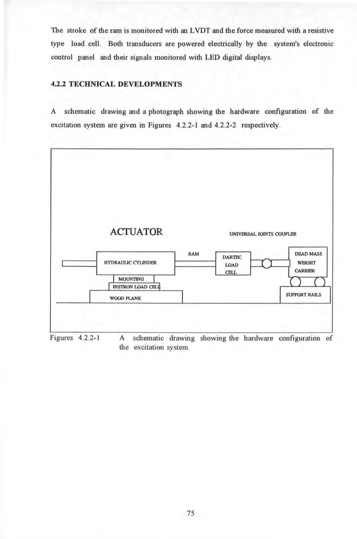
UNIVERSAL JOINTS COUPLER
RAM DARTEC DBADMASS HYDRAUUC CYUNDBR LOAD r] WEIGHT CElL CARRIER I MOUNTING I ) ( )
l lNSlRON LOAD CBUJ I I I SUPPORT RAILS WOOD PLANK
Figures 4 2 2-1
A schematic drawing showing the hardware configuration of the excitation system .
L
I
75
Figures 4 2 2-2 A photograph showing the excitation system

Several items were added to the basic actuator to turn it into a fllllctional exciter. The various 'add-on' components were :
a mollllting
a react10n mass and its support and
a coupler
A special mounting arrangement was designed and manufactured. 1l1is is a trunnion type mounting made from two square steel plates with one plate capable of sliding over the other and turning about a centre pivotal steel pin The top plate has two semi-circular slots cut into it to allow bolts to go through and be secured onto the bottom plate . The bottom plate has ho les at the four corners to receive the bolts from a wood plank which is glued to the floor of a tested structure. This arrangement allows the actuator to be turned to some other directions while in its secured position
The final design of the reaction mass assembly was affected by a number of functional considerations. 1l1e dead masses were made from lead because of its high density . They
76
were cast as flat plates of approximately 15.5 Kg weight each. A steel handle and a slot was provided for each plate for easy loading and unloading from a weight carrier.
The weight carrier used for carrying these lead plates was a very sturdy unit made in the form of an open-box trolley with two steel plates welded at the two ends. A threaded screw rod was welded to the two end-plates. The lead plates were slotted one by one along the rod and through the slotting hole when loading. Two steel backing plates sandwiched the lead plates and were secured by two nuts at each end. Different numbers of plates, up to a maximum of 12, could be placed in the carrier to fulfil different force requirements.
The carrier was supported underneath by four linear ball bearings which ran on two rails with high quality surface finishes. These arrangements were instrumental in reducing nonlinear Coulomb friction.
A 'flexible' coupling joint was introduced between the carrier and the ram in order to eliminate any lateral load introduced to the ram which could damage the hydrostatic bearings. This coupler is a short 'push-rod' with universal ball-and-socket joints welded at both ends. An attachment freed from backlash is achieved by using two fme precision slotting pins. This coupling arrangement allows some vertical and horizontal misalignments between the ram and the carrier.
4.2.3 PERFORMANCE TESTS
Tests were carried out to determine the performance of the entire system in the low frequency range (i.e. 5 Hz or below) : not only the actuator system itself but also the other attachments to it. Performance in terms of the maximum force produced, the practical limits in stroke, acceleration etc of the ram in relation to driving frequencies was investigated. To eliminate other possible influential factors which might affect the performance of the actuator, simple sinusoidal instead of random or transient driving signals were used. Although the actuator allowed two modes of operation under either load or stroke control, only the latter was used. Details of this control can be found in the manufacturer's operation manual 14 .q Some of the results from these tests are plotted in Figures 4.2.3-1 to 4.2.3-3.

77

3o.oo I l s- 25.00 20.00 !":I.. 0 15.00 z 0 ' ! ' -+ 1o.oo ____ T _____ ' ij 0.00 0.0 1.0 2 0 3.0 4.0 5.0 6.0 7.0 8.0 INPUT CONTROL VOLTAGE VOL'IS - 1HZ ---+- 1.5 HZ -e- 3 HZ ---¥- 4 HZ -A- 5 HZFigure 4.2.3-1
0.5 1 STROKE (RAM OF EXCITER) 1.5 2 2 .5 3 3.5 4 4.5 5 5 .5 6 6.5 7 7 .5 INPUT CONTROL VOLTAGE VOL'IS - 1HZ ---+- 1.5 HZ -e- 3 HZ ---¥- 4 HZ -A- 5 HZ
78
ACCELERATION (RAM OF EXCITER)
Acceleration resJX>nses of the loaded ram of the actuator over a range of input voltages and frequencies.
Figure 4.2.3-2 Stroke responses of the loaded ram of the actuator over a range of input voltages and frequencies.
FORCE AMPLITUDE GENERATION BY EXCITER
Figure 4 2 3-1 shows that the maximum accelerations allowed are 25 and 15 m/s2 at 5 and 1 Hz respectively . These maxima stay the same for each of the frequencies even with further increase of the input voltages . Figure 4 .2.3-2 show that the maximum strokes allowed are only 30 mm at 5 Hz which fall short of the 420 mm allowed at 1 Hz. The marginal decrease in the allowable maximum stroke is more subtle at low er frequencies.
Figure 4.2 .3-3 shows that the maximum force generated is 5 KN when driving at 5 Hz. No further increase in force is allowed when the input voltages exceed 4.5 Volts. These figures all show that if the control voltage is well below the maximum input voltage allowed (i e the capacity of the hydraulic system is not exceeded) then the performance of the exciter is essentially lin ear All these maxima are governed mainly by the characteristics of the hydraulic actuator such as :
the maximum supplied oil pressure
the maximum oil flow rate and
the effective bore area of the ram

6.oo I i 5.00 I MAXI LOAD I s 4.oo , ___ J_ -L---. : .... I i 3.00 i - ----..• l l ::E 2. 00 ! +··--·-·--1-----r--··u _ j __ I ___ 1.00 0.0 1.0 2.0 3.0 4.0 5.0 6.0 7.0 8.0 INPl.IT illNTROL VOLTAGE VOLTS 1 HZ --+- 1.5 HZ 2 HZ -a- 3 HZ 4 HZ _.__ 5 HZ
Figure 4.2.3-3 Load generation capability of the exciter over a range of input voltages and frequencies.
79
In these tests, the driving signal feeding the control panel was obtained from the Philips signal synthesizer. Whilst this signal might be regarded as a relatively pure sinusoid, the effects such as due to the nonlinear characteristics of the hydraulic exciter and its attachments which produced forces with the significant presence of harmonic components. These harmonics had frequencies of integer multiples of the forcing frequency. This was particularly so when the exciter was operating at conditions close to the limits imposed by the pumps, electronic valves etc.
4.2.4 CALmRATIONS
A series of calibration tests were carried out to determine the relationships between the measured force from the DARTEC load cell and the actual shear force transmitted through the mounting and measured with the INSTRON load cell.
The ratios between the forces measured by the two transducers were determined using sinusoidal as well as PRBS (Pseudo-Random Binary Sequence) forces. The results show that these ratios (DARTEC reading over INSTRON reading) can vary from 1.04 to about 1.06 in sinusoidal tests, and from 1.05 to 1.06 in PRBS tests over a range of frequencies from 0 to 25 Hz and ·a combination of different loading conditions. Further information CaD be fc:>und in Reference 1431 So an average of 5 % error is expected if load is taken from the DARTEC instead of the INSTRON load cell.
4.3 SENSORS AND TRANSDUCERS
The sensors and transducers required were naturally fallen into two categories I.e. those concemmg:
a. the operation of the exciter and

b. the responses of a structure.
4.3.1 STROKE MEASUREMENT
The proper operation of the exciter requires the stroke of the ram to be monitored at all times to ensure the satisfactory running of the actuator under the stroke control
80
mode. An LVDT (linear voltage differential transformer) was used for this purpose. The L VDT output signal is frequency modulated using a 5 KHz carrier. An LED digital display of the stroke is provided in the control panel.
4.3.2 ACCELEROMETERS
4.3.2.1 DESCRIPTIONS
The acceleration response of a structure was measured with servo-driven closed-loop torque balance SCHAEVITZ accelerometers. With the servo-control mechanism, these accelerometers are capable of working with DC signals which most piezoelectric types of accelerometers cannot. The transduction principle and details of the operations of these accelerometers can be found in Reference 1431 These accelerometers are externally powered so that they can be made very light and small. A special power pack and a junction box provide the required electrical power and cable connections. When used in the field, each accelerometer was screw-mounted on a heavy metal block for stability. Each accelerometer has a sensitivity axis which is to be aligned along the intended response direction. Apart from the sensitivity direction, each accelerometer has also got a cross-axis sensitivity which is usually only a small value and no special considerations are required.
4.3.2.2 CALffiRATIONS
The accelerometers were calibrated both statically and dynamically. As these accelerometers are designed to work with DC, static gravimetric calibrations were performed using the Earth's gravitational field. These were carried out by placing the accelerometers on a sine table which could be tilted about a base to very precise angles. The corresponding voltage outputs from the accelerometers at various angles were used to calculate their sensitivities.
Dynamic calibrations were carried out by placing all the accelerometers side-by-side on the weight carrier. The ratios of the corresponding voltage outputs from each of the accelerometers and those from the LVDT were used to calculate their sensitivities. In taking these measurements the exciter's ram was set to wide band random motion.
The results of the calibration are summarized in Table 4.3.2.2-1.

81
TABLE 4.3.2.2-1
COMPARISON OF THE EXPERIMENTAL AND THE MANUFACTURER'S CALIBRATION OF THE ACCELEROMETERS.
The results show that the sensitivities of the accelerometers are ranging from 2.396 to about 2.490 (Volts/g) whicb are .quite close to those specified by the manufacturer. The calibration had resulted a set of liqear coefficients which were all very close to one. The linear regression is a measure of the linearity between voltage outputs and the corresponding sine of angles of tilt. This coefficient normally has a value ranging ·. between 0 and i. A coefficient of 1 indicates perfect linearity.
4.4 SIGNAL CONDITIONING AND PROCESSING
4.4.1 GENERAL SIGNAL CONDITIONING

Very often and especially in the field, the pick-up signals were weak and noisy. Signal conditioning was required before these signals could be read and recorded. Simple signal conditioning operations sucb as amplifying, DC off-setting and low-pass filtering were provided by an integrated electronic hardware.
Because of the inadvertent production of a small DC output when an accelerometer was not aligned properly on a horizontal plane, offsetting this DC output was required. Providing the magnitude of this DC signal was not too excessive, most modem signal processing equipments could cope with this situation because of the wide dynamic range
Accelerometer serial number 1650 1652 1653 1654 1658
Sensitivity Linear regression Manufacturer's volts/g coefficients calibration 2.442 0.9981 NO RECORD 2.454 0.9999 2.534 2.490 0.9998 2.531 2.450 0.9997 2.521 2.396 0.9998 NO RECORD
82
and high sensitivity they have. The HP 3582A spectrum analyzer has a 75 dB dynamic range to spare. So DC offset operation was often waived in return .for a speedy measurement.
4.4.2 SIGNAL RECORDING
4.4.2.1 ANALOG TAPE RECORDING
The outputs from various transducers were analog voltage signals and were recorded using a RACAL instrumentation tape recorder. The recorder was a four channels FM tape recorder with a range of selectable recording speeds. A speed of I 5/16 inches per second was chosen for most recordings. At this speed, the recorder has a useful bandwidth from DC to about 300 Hz. Details of the operation of the recorder can be found elsewhere 14 .41 Tape recording was used for backup only.
4.4.2.2 DIGITAL DATA RECORDING
Handling and processing data recorded as analogue signals was very troublesome and inefficient. Digital data which are not only easy to transfer from one recording medium to another but also provide high fidelity of transfer. In Section 4.5, the details on the digital processing and recording of data utilizing a desk-top computer will be described.
4.4.3 EXCITATION SIGNAL GENERATION

4.4.3.1 SINUSOIDAL SIGNALS
The ram's motion is under the control of the input signal fed into the DARTEC control panel. These signals, and hence the ram's motion, could be sinusoidal or random. An internal sinusoidal signal generator is provided as an integral part of the control panel for this purpose. However an external signal source, a Philips PM 5190 programmable Low Frequency signal synthesizer, was used instead. Sinusoidal signal generation in the synthesizer is based on digital algorithms rather than crystal oscillations. This equipment can either be controlled from the front-panel or remotely via an IEC 625 interface. Signal frequencies are selectable from l MHz to 2 MHz, and AC voltage levels are also selectable from 0 to just below 20 Volts. It also allows an option of imposing an intended DC
83
bias voltage over the preset AC voltage levels . Details of the operation of the generator can be found elsewherel 4 .5J _
4.4.3.2 PERIODIC RANDOM SIGNALS
A periodic random noise generator is provided by the Hewlett Packard spectrum analyzer which is shown in Figure 4.4 3 2-1. This noise source is functionally equivalent to a tracking generator with 256 parallel oscillators. The f r equencies of these oscillators coincided with the 256 spectral lines provided by the analyzer. A carefully matched uniform pass-band filter is built in the analyzer. The signal generation is based on the use of a recursive Pseudo Random Binary Sequences (PRBS) shift registers and implemented in hard-wired chips The exact details are outside the scope of this review and other references on signal generation techniques should be consulted .

4.4.4 SPECTRAL ANALYSIS
The power of modem signal processing techniques lies in the capability to perform Discrete Fourier Transform (DFT) on discrete, sampled time data of finite block length . DFT is an implementation of the Fast Fourier Transform (FFT) to extract spectral
Figure 4.4 .3 .2-1 The Hewlett Packard HP 3582A spectrum analyzer.
84
information from sampled time data. Equipment with such capability is called a spectrum analyzer, or a Fourier analyzer. The analyzer used in this investigation was a Hewlett Packard HP 3582A dual channel real-time spectrum analyzer. A brief description of the signal processing performed in the analyzer is given below.

Incoming signals are first passed through an analogue 25 KHz low-pass filter. This filter eliminates any energy in the signals due to frequencies higher than the fastest sampling rate. Failure to do so produces aliasing (see Ewins 15 10 1 for a concise description). The filtered signals are then passed through an analogue-digital-converter (ADC) which has 12 bits precision of conversion.
Further digital filtering is performed by four Large Scale Integration chips which can be considered as a cascade of eight distinct filter stages as a close analogy. Each stage of the filter reduces the incoming signal bandwidth by a factor of 2 or 5. The ADC is set at a sampling rate of I 02.4 KHz i.e. 102400 samples per second. The filtered time sequences are then stored in the time buffer until a full I 024 data points (data block length for single channel) or 512 (for dual channels) are recorded.
The time domain data are then 'windowed' which can be considered as a process of 'point-by-point' multiplication of the digitized time data and the stored weighting functions appropriate to the window selected. A suitable window has to be selected in relation to the types of signals encountered. Windowing suppresses a signal processing problem known as leakage (see Ewins ''·10 1 for a concise description).
The DFT computation is performed by a 16 bits built-in micro-processor inside the analyzer. The computed spectral data are then stored in the frequency buffers and can be called up for display on the analyzer screen. Averaging is also performed to improve the quality and accuracy of the measurements. A good selection of different averaging facilities are provided by the analyzer : such as time or root-mean-square RMS spectral averaging. Further information regarding the operation of the analyzer can be found elsewhere f4.6f,f4.7) and f4.8l.
4.5 COMPUTER-AIDED-TESTING (CAT)
Labour and time intensive manual testing techniques are no longer adequate for the new
85
advanced methods. The advent of instrumentation technologies, and the successful miniaturization of computer hardware bring CAT from the laboratory to the field. Automation in data acquisition and recording can now be carried out in the field. Many more commercial systems are now available from well known manufacturers such as: Bruel & Kjaer, Solartron or Structural Dynamic Research Corporation etc. However this research had not have the opportunity of obtaining any one of these systems. Instead a system of very low cost was developed in-house.
4.5.1 THE HARDWARE CONFIGURATIONS
Basically, the CAT system was built upon the integration of several stand-alone instruments with a Hewlett Packard HP 86B micro-computer (a schematic of this system is shown in Figure 4.1-1 ). The resulting costs were low if the costs of software developments were discounted. The extra costs on the hardware required was small.
The physical integration was achieved by interfacing the computer, its peripherals and other remotely controlled ('remote control' is used here as a contrast to local'front-panel' control) equipments via an IEEE 488 Interface, or otherwise known as the Hewlett Packard Interface Bus (HPIB). The IEEE 488 bus is one of the most popular universal interface standards which unify both the hardware and software interfacing requirements. This standard has been adopted by most instrument manufacturers in their products. Other standards such as the European IEC 625 or the RS 232 are also used.
Equipments with the same interface can simply be plugged together with suitable cables and connectors. Equipments complying with different standards can also be linked together provided suitable adaptors are used. These adaptors are more than just merely a device for mechanical compliance. A special adaptor was made to enable the interfacing of the PHILIPS signal synthesizer, which is based on the IEC 625 standard, to the IEEE 488 based bus.
On the HP 86 computer, this interface capability is supported by an input/output interface cartridge (an HP 82936A 1/0 ROM Drawer). In essence, this cartridge allows the computer:
a. to address to each interfacing instrument,

86
b. to perform controls and data input/output operations using high level programming languages rather than low level machine languages and
c. to perform 'handshaking' according to the designated protocols during data transmission.
4.5.2 THE CONTROL PROGRAMS
The test sequences and the associated controls were coded as a computer program. This control program was written in extended HP BASIC and was designed and written in a modular structure so that future modifications and additions could be done easily. The running of the program was menu driven and an operator's intervention was kept to a minimum. This program was capable of the following tasks :

a. Remote setting up of equipments (this was done by sending appropriate sequences of the HPIB interface commands from the computer to the various instruments via the IEEE 488 bus).
b. Interrogation of the status of the measurement process, for instance to check if overloading had occurred (this was done by interrogating a particular bit in a special memory register chip inside the HP3582A analyzer)
c. Recording digital data and spectral displays from the analyzer onto magnetic disks for storage {this was done by down-loading sequences of bits from the special memory registers inside the HP3582A analyzer which held the spectral and screen display data).
As a result, testing could be performed much more speedily than before and large quantities of useful data could be acquired with very little attention from the operator. Generally, this CAT system is beneficial to the experimentation process in a number of ways:
a. It eliminates the tedious tasks of manual recording and switching.
b. It increases the speed of data recording, retrieval and storage
87
c. It makes immediate on-site processing possible for preliminary checking of data.
d. It allows data transferability from one to another computing environments between micros, PC or main-frame computers. The latter is particularly useful for very large scale data processing and calculation.
Details and listing of the control program are given in APPENDIX 4.5.2.

4.6 SUMMARY
A new excitation mechanism was developed and its performance checked. Generally, the exciter has to be operated well within the operating limits otherwise non-linear distortions will result. The sensors were all calibrated so that measured data can be converted to their real physical units. The force read by the Dartec load cell have a +5% error relative to the load transmitted to the mounting. A low cost but powerful CAT system was successfully developed and could be put to use in the field.
88
CHAPTER 5
EXTRACTION OF MODAL PARAMETERS FROM FORCED VIBRATION DATA
5.0 INTRODUCTION
This chapter is specifically concerned with the methods of.extraction of modal parameters to obtain a modally truncated model of a real structure. A modally truncated model is defmed as a modal model which is representative of the effects of a small number of identifiable modes within a limited frequency band only (instead of an infmite number of modes a continuous structure might have). The effects of the modes outside this frequency band is called the 'residual' effects This will be explained more clearly when dealing with the receptance frequency response function in series expansion form in Section 5.1.1.
A brief reVIew of some conventional methods will be given first and followed by the presentation of an alternative algorithm developed by the author. This algorithm is based on direct least-square fitting technique and shares some similarities to the dynamic stiffness method. An exercise to compare this algorithm with two commonly used methods was carried out and the results are reported. Modal parameter extraction is an essential process in the derivation of a modal model of a structure. The validity of this model depends very much on the capabilities and accuracies of the methods used in this process.
An assortment of methods is in existence nowadays. Broadly speaking, most of the popular methods used today can be categorised according to the types of data required for the operation. Those methods which work with time or frequency data are known as the time and frequency domain methods respectively.
89
In the early days when sophisticated instrumentation and digital computers were not available, the process of modal parameters determination could only be carried out by simple and rudimentary means. In those days, the data obtained were often in analogue form: such as magnetic signals on tape, strip charts or hand written readings and hence they were difficult to process.
Many early methods, such as the so called 'peak picking' method, were based on visual inspection and on simple arithmetic calculations to a large extent. The frequencies corresponding to the peaks in an FRF spectra (the resonance frequencies) give an estimate of the undamped natural frequencies. The modal damping factors were often determined using either the 'half-power' or the 'logarithmic decay' methods. All these methods did not require phase measurements and relatively simple instruments were adequate for their implementation. Much of the work carried out during the 1960's and the 1970's was based on these methods. In fact, many of these methods are still being used today.
With the introduction of better instruments, more sophisticated analysis methods have been employed. In particular, phase information allowed additional criteria to be used for modal parameters determination. For instance, the undamped natural frequency of a system with well separated modes (i.e. the assumptions of SDOF hold) can be located on the frequency axis corresponding to :
a. the peak (or trough if negative) in the imaginary part of an FRF Bode plot,
b. the maximum rate of frequency-swept-through-an-arc of a resonance circle in a Nyquist plot,
c. zeros in a real component FRF Bode plot or
d. 90 degree phase angle changes in phase FRF Bode plots
A string of methods were also available for the determination of other modal parameters using phase information. Schiff had given an excellent account of the numerous methods of this category and further details can be found in this reference.
With the availability of even more powerful instruments, more sophisticated methods

90
have been applied. Most of these advance methods performed a process known as 'curve-fitting'. In essence, the object of this process is fitting measured data to a postulated mathematical model. Most of these methods apply least-square-fitting technique in one way or another.
Another broad categorization of the various methods can be made according to the number of modes assumed in this curve-fitting process. Methods which curve-fit a single mode at a time or a multitude of modes simultaneously are termed SDOF-fit and MDOF-fit methods respectively. Some methods, which perform this curve-fitting process by utilizing data from all measurement locations in a single run, are termed the global methods.
5.1 CONVENTIONAL METHODS
As already mentioned, most methods can be classified as Time Domain (TD) or Frequency Domain (FD) methods. In general, most TD methods require time data captured from the transient responses of a structure subsequent to an impulsive type excitation. Because these transient events (measured as a series of wavefom1s) usually happen only within a very short period of time, specialized equipments, such as a transient recorder capable of high sampling rates, are required. These waveforms have to be recorded at very closely spaced discrete instants of time in order to satisfy temporal and hence spectral resolution requirements. Furthermore, simultaneous recording of all the measurement locations of a structure are sometimes mandatory as in the case of multi-input methods. All these factors impose specific and often formidable requirements on data acquisition as well as analysis.
FD methods here refer to those methods which are often carried out with steady-state stepsine, slowly or rapidly swept-sine (also known as 'chirp'), multi-sine, periodic or periodicrandom type of excitation. Spectral frequency response data are then obtained from sampled time data via Discrete Fourier Transformation (DFT). The spectral resolution and accuracy of this transform depends on the various signal processing operations involved such as: selection of the rate of sampling, block length of time series, windowing, anti-alaising filtering, averaging and so on appropriate to the test conditions. Because this study is mainly concentrated on FD methods, no further discussions of TD methods will be given here. Readers interested in the various TD methods such as: the Least Square Complex
91
Poly-reference I'-'I and lbrahim m methods ' 5 6 1 can consult the original papers cited in the references. In particular, two papers by Cooper 15 71 and Fullekrug 15 "81 have given a general survey and comparison of these TD methods and are useful references.
The most frequently used model, using SISO (as introduced in Section 3.3.2.1), is the series representation of receptance of a multi-degree-of-freedom system:
5.1-1
where Y; is the hysteretic damping loss factor ffi; is the undamped natural frequency
G• i is the complex modal constant
N is the total number of degrees of freedom (or modes) of the system subscript i denotes the ilh mode of vibration subscript sr denotes response at coordinate s and force at coordinate r j is the imaginary unit v-1
This equation is often considered as the keystone to the understanding of modal analysis which stipulates that receptance at any frequency is a summation (or superposition) of the contributions of all the system's modes at that frequency. As this is a rather important equation, a short derivation is given. The equation of motion with hysteretic damping matrix [H] is often quoted as:
The homogeneous solution to Equation 5.1-2 is again an eigen-value problem:
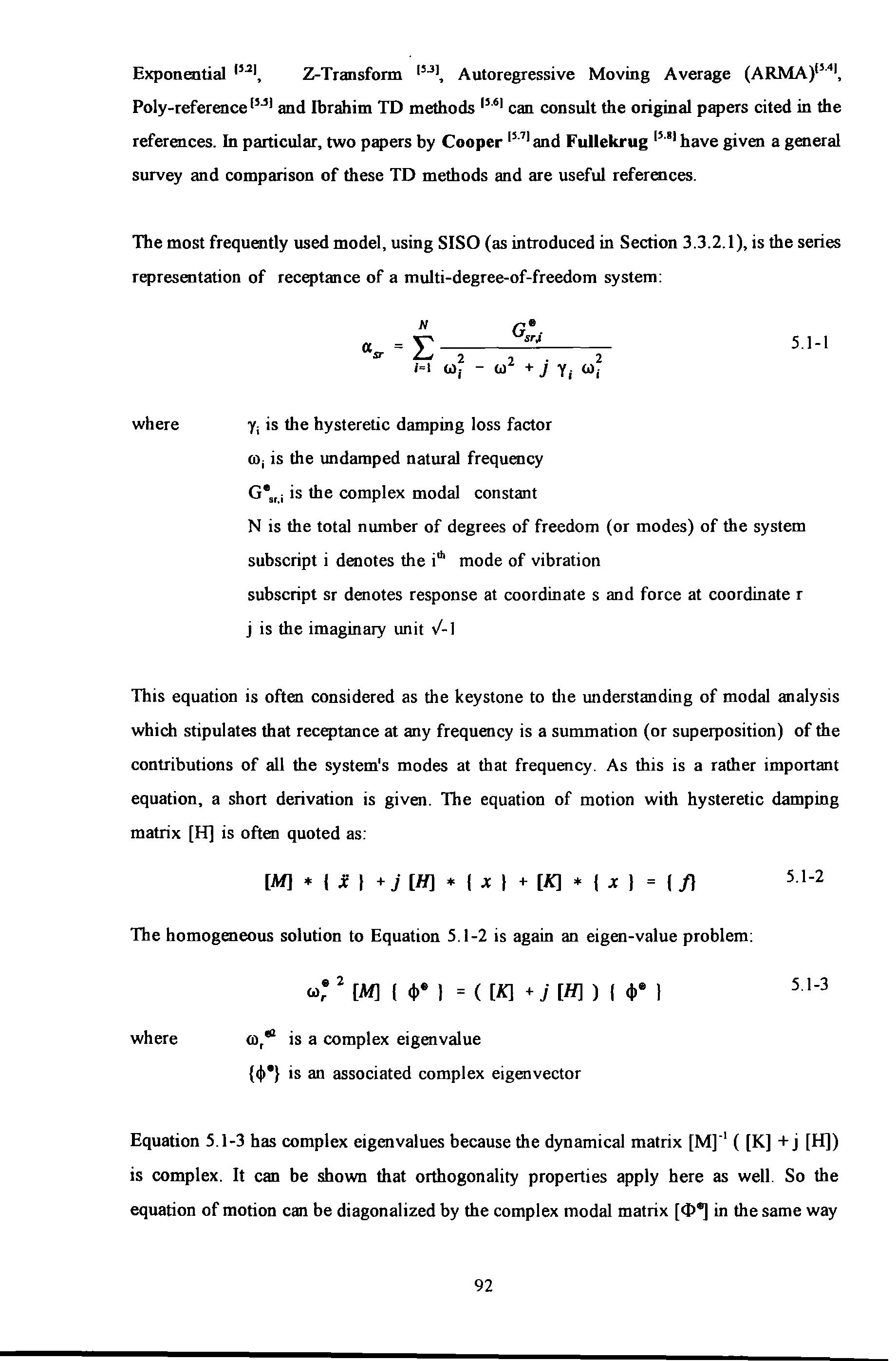
where ro, ell is a complex eigen value
{cjl 8 } is an associated complex eigenvector
Equation 5.1-3 has complex eigenvalues because the dynamical matrix [Mr' ( [K] + j [H]) is complex. It can be shown that orthogonality properties apply here as well. So the equation of motion can be diagonalized by the complex modal matrix [<I>, in the same way
Exponential ' 52 1, Z-Transform JBJ, Autoregressive Moving Average (ARMA)15 · 41 ,
[M] * I X I + j [H) * I X I + [K] * I X I = I 11 5.1-2
2 [M] I ell• I = ( [K] + j [H) > I ell• I 5.1-3
92
as the undamped modal matrix [<I>] in the undamped case. Hence:
Where [M*], [K*] and [H*] are all diagonal matrices. In the forced vibration case, the frequency response function is obtained by applying Fourier Transform to Equation 5.1-2:
Pre-multiplying by [<I>,T and applying the modal transformation to Equation 5.1-5 to obtain:
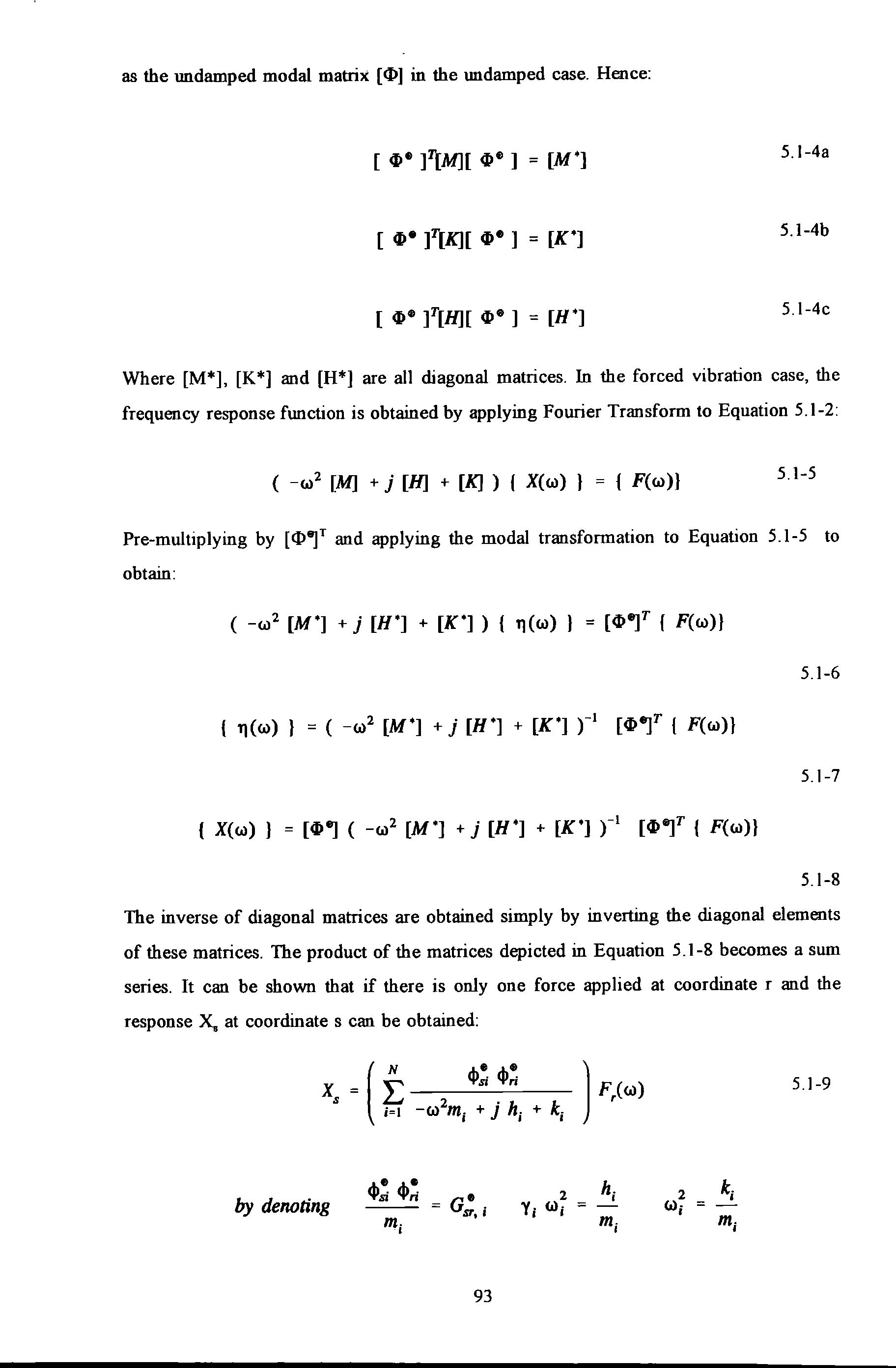
The inverse of diagonal matrices are obtained simply by inverting the diagonal elements of these matrices. The product of the matrices depicted in Equation 5.1-8 becomes a sum series. It can be shown that if there is only one force applied at coordinate r and the response X. at coordinate s can be obtained:
by denoting
[ «>• ]l(M][ «>• ] = [M•] 5.1-4a 5.1-4b 5.1-4c
( -w 2 [M] + j [H] + [K] ) ( X(w) } = { F(w)} 5.1-5
{ -w 2 [M•] + j [H•] + [K"] ) { TJ(W) } = [«>e_)T ( F(w)} 5.1-6 ( T)(W) } = ( -w 2 [M•] + j [H•] + [K"] r 1 [«>e_)T { F(w)} 5.1-7 ( X(w) ) = [«>8_1 ( -w 2 [M•] + j [H•] + [K"] r 1 [«>e_)T ( F(w)} 5.1-8
5.1-9
93
The expression in bracket is in fact receptance a. as depicted in Equation 5.1-1.
5.1.1 SDOF-FIT METHODS
SDOF-fit methods are all based on the assumption that in the vicinity of the natural frequency of a mode on a frequency axis, the total response of a structure in this frequency band is dominated by the effects of that mode alone and those from the neighbouring modes are either negligible or their effects can be represented collectivel y by complex residuals So considering frequencies close to the natural frequency of the ilh mode, receptance can be represented by (note that the summation sign is dropped) :
The first term on the right hand side of the equation represents a circular loci in an Argand plot which will be exp l ained further in Section 5. 1.1. 1. The second term (a+bj) is the complex residual. This assumption work s well for a structure with well-separated modes i e. low modal density
SDOF-fit methods are amongst the most widely used methods which can o ft en be carri ed out by simp le graphical techniques or e lementary arithmatic manipulation of dat a. Som e methods uti lize certain geometricall y realizable forms , such as straight lines and circles, exhibited by the data o n special plots as the criteria for the determination of the modal parameters. They are usually referred as the Circle-Fit and Straight-Line-Fit methods respectively. S ince these two meth o ds had bee n used in th e comparison exercise reported in Section 5.4, the theoretical basis of these two methods is to be expanded in
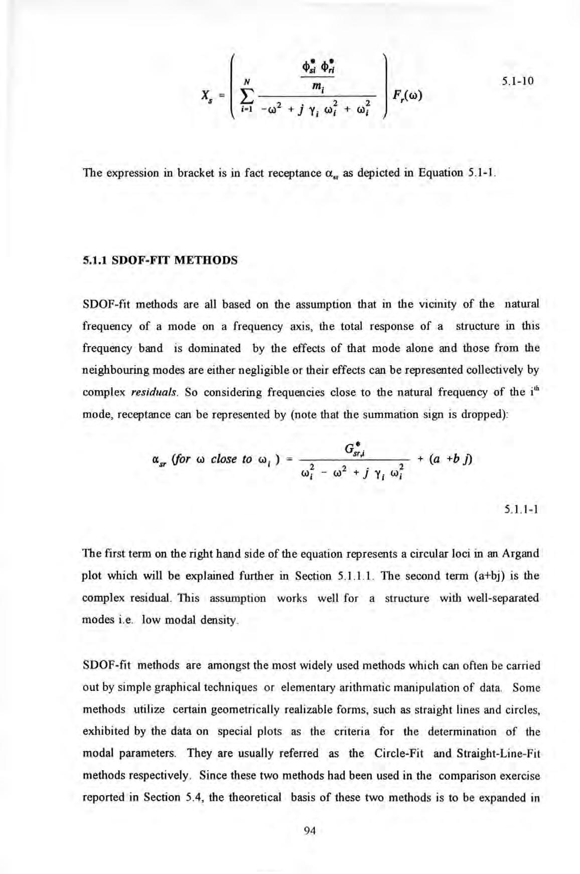
4>: N m; 5.1-10 xs L Fr((t)) - (1)2 2 2 i =l + j Y; (t); + (t)j
2 2 . 2 W; - (t) + J Y; (t)j + (a +b J) IXsr {for (t) close to (t); ) 5 1.1-1
94
slightly greater details below.
5.1.1.1 CIRCLE-FIT METHOD
This is a method due to Kennedy and Pancu 15 91 In this method, the real (coincident) part are plotted versus the imaginary (quadrature) part of the complex receptance or mobility data in an Argand plane This plot is usually known as a Nyquist plot. By choosing the duality appropriately : i .e . a suitable damping model and the type of frequency data used (receptance a for hysteretic damping as given in Equation 5 1.1-1 , or mobility p for viscous damping), the lo ci traced by the data points, which clustered around the regions of resonance, are in the form of a seri es of arcs of circles A thorough exp lanation of the use of this method has been g iven by Ewi n s 15 101
The accuracy which can be achieved by thi s method is found to be quite sen s itive to two factors : i e the levels of noise in the data and frequency resolution between consecutive data points Noisy data points will show up wandering irregularly , or randomly in the case of random noise , away from the true circle Apart from random measurement noise , it is a known phenomenon that near resonance, the force amplitudes drop while the response amp litudes increase drastically. The large disparity between their magnitudes (or s ignals) causes measurement errors. Therefore the measured receptance can be highly 'contaminated' with noise in these circumstances This problem is often reflected by showing a very low cohere nce b e tween excitation and response near resonance

The effects of frequency resolution will , in turn , depend on the levels of damping . At one extreme, lo w damping 'coupled' with insufficient frequency resolution will cau se the data point to cluster together near the origin with sparsely distributed points or none at all to map out the rest of the circumference of a circle At the other extreme, high dampin g 'coup led' with high frequency reso lution will caus e the data point to spread around closely along the loci of circles When applying Circle-Fitting procedure to the first case i e poor mode resolution , the modal parameters determined wi ll be erroneou s
The circle traced by the data points, based on the first term of Equation 5 1.1-l alon e but with real modal constant, is symmetrical about the imaginary axis and the circle passes the or igin of the Argand plane as shown in Figure 5 . 1.1.1-1. In the case having a comp lex modal constant, the axis of symmetry wi ll no longer be the imaginary axis but an ax ts
95
turned at an angle about the origin. Finally, the effects of the residual merely displace this circle by a vector (a+bj) in the Argand plane.
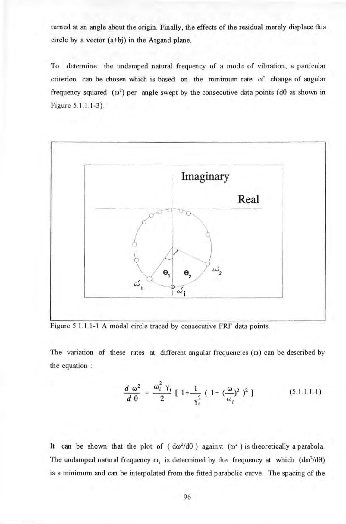
To determine the undamped natural freq uen cy of a mode of vibration, a particular criterion can be chosen which is based on the minimum rate of change of angular frequency squared (ro 2 ) per angle swept by the consecutive data points ( d8 as shown in Figure 5 1 1
The variation of these rates at different angular frequencies (ro) can be described by the equation : (5.1.1.1-1)
It can be shown that the plot of ( dro 2/d8 ) against ( ro 2 ) is theoretically a parabola The undamped natural frequency ro; is determined by the frequency at which (dro 2/d8) is a minimum and can be interpolated from the fitted parabolic curve . The spacing of the
cJ 2 Real
1-3)
Imaginary
Figure 5 . l.l.1 - 1 A modal circle traced by consecutive FRF data points .
96
two neighbouring frequency points (corresponding to w1 and W2 ) on either side of the frequency point corresponding to wi on a modal circle can be used to determine the hysteretic damping loss factor Yi by using the following equations :
Y; 2 W; e TAN (1 ) 2
1 e + 2
5 1.1.1-2)
where 6 1 , w1 , 6 2 and w2 are shown in Figure 5 1.1.1-1. To determine the magnitude of the complex modal constant IG•.r.i I , the following equation is used :
(5 . 1.1.1-3)
The general problems associated with the circle-fit methods are :
a The data points around a resonance have different weighting in the effectiveness of defining the Nyquist circle of a mode Data points further away from a resonance tend to cluster around the origin of the Argand plane rendering them less effective than those closer to the natural frequency of the mode. However, data measured near resonance is less accurate and more 'noisy' as explained earlier.
b Measurement of angles subtended by data points near resonance is very difficult to be accurate (for very much the same reasons as in a) Hence considerable errors result in estimating the hysteretic damping loss factor.
c. The three modal parameters have to be determined in a prescribed order. So errors in determining one parameter can be accumulated in and propagated to the determination of the next parameter and so on .
5.1.1.2 STRAIGHT-LINE-FIT METHODS
It is generally known that plotting the real and imaginary parts of the inverse of receptance (called 'dynamic stiffness') against the square of angular frequencies ( w2 ) will produce
97
straight lines (see Ewins 1'·131 ) The theory is based on the formulation (by dropping the effects of residual and assuming proportional damping i.e. real modal constant) :
This straight-line techniqu e using dynami c stiffness data ha s been proposed by a number of researchers : s uch as Goyder 15 111 and Dobson 1'·121 (see further remarks given later in this Section). Full details of the specific application of this method can be found in the cited reference Using dynamic stiffness method, the modal parameters of each mode can be determined from the geometry of these straight lines (i .e. the slopes and intercepts) corresponding to each of the respective modes of vibration For instance, the undamped natural frequency ro; can b e identified as that at which the straight line in the real plot intercepts the ro 2 axis The modal constant can then be determined using the equation :
Because the plot of the imaginary part of dynamic stiffness against ro is also a straight line with zero s lop e and the intercept on the vertical axis can be used , in conjunction with the previously estimated modal constant and natural frequency , to determine the hysteretic damping coefficient Y; using the following equation :
Notice that Equation 5 1.1. 2-2 is only true when residual effects fr om the out of range modes are neglected. Hence raw data h ave to be pretreated before they can fit th e straightline model. The pretreatment necessary is that prior to inverting these data to obtain dynamic stiffness data , the residual term (a + bj) has to be determined first and then subtracted from the raw receptance data (as stipulated in Equation 5. 1. 1- 1) before. One such
1 2 2 . 2 W; - (J) + 1 Y; W; a sr (for (J) close to (J) i ) Gsr,i 5 1.1.2-2
- 1 ( SWPE OF THE STRAIGHT] UNE IN THE REAL PWT (5 . 1.1. 2-3)
( OFFSET OF THE STRAIGH1) 1 Y; = Gsr,i * UNE IN THE IMAG PWT ) * 2 W; (5 1.1.2-4)
98
method is by determining the complex vector of displacement of the Nyquist circle in the Argand plane as explained in Section 5. 1.1.1.
The method by Dobson IS tlJ in particular, utilises the difference equations technique which has some advantages over the conventional dynamic stiffness method This method can apply to a non-proportionally damped system (i e system with complex modal constants) whil st conventional methods assume a proportionally damped system This method provides a direct determination of the complex residual as part of the fitting routine without the need to estimate the residual by separate means which is requir ed as a pre-requisite with the conventional methods ( s ee Dobson (s tll for full detai ls)
5.1.2 MDOF-FIT METHODS
MDOF-FIT methods refer to those which perform a multi-modes-curve-fit in a single step which is in contrast to the iterative step s used in SDOF-FIT methods . Some MDOF methods are also called 'global' methods becaus e these methods can perform curve-fitting to the global set of FRF data from all the measuring positions in a single run . Most methods stem from the assumption that the FRF of a linear second order dynamical system can be represented as a ratio of two polynomial functions with unknown parameters ak and bk (totalling m+n + 2 in number , where m = 2N-l, n=2N and N =total degree-of-freedom of a system) . As a convention, b" is chosen as Wlity (a condition which can always be satisfied by appropriate factorization) Therefore only (m+n + l) parameters need to be determined As a rule, the value n is usually chosen as 2 times the number of modes present while the rule to fix the value of m is less certain . m
I: a s* * H(w) k=O 11 where s = j w (5 1.2- 1)
I: b s* * k=O
By convention, H( ro) is usually expressed as the sum of a rational fraction polynomial (i .e. n >m) and extra terms which accoWlt for the out-of-rang e modes's effect. A string of methods use different varieties of this formulation will be further explained below.
99
5.1.2.1 PARTIAL FRACTION METHODS
As a natural extension to the formulation in Equation 5.1.2-1, it can be rewritten in terms of partial fractions :
where
where crk and are damping coefficient and damped natural frequency respectively .
This approach again has a very strong origin from control engineering It is evident from Equation 5 .1.2. 1-1 that this equation contains 2n+2 unknown parameters : rk> r·k and p ·k for each of the n modes within the analyzed frequency band together with two residual parameters accounting for the residual effects of the out- of-range modes .
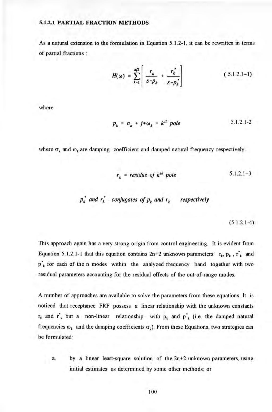
A number of approaches are available to solve the parameters from these equations . It is noticed that receptance FRF possess a linear relationship with the unknown constants and r·k but a non-linear relationship with and p·k (i e the damped natural frequencies rok and the damping coefficients From these Equations, two strategies can be formulated :
a . by a linear least-square solution of the 2n +2 unknown parameters, using initial estimates as determined by some other methods ; or
( 5.1.2.1-1)
5 1.2 1-2
rlc =
5.12.1 - 3
(5 .1.2 . 1-4)
residue of kth pole
P1c• and rlc· = conjugates of P1c and rlc respectively
100
b. by iterative nonlinear least-square solutions to all the unknown parameters.
Clearly the accuracy of these methods depend very much on the accuracy of the initial estimates. A poorly chosen estimate will often lead to divergence from the true solution. Further details of these methods have been documented by Van Loon IH41
5.1.2.2 GLEESON'S METHODS
For very lightly damped structures , Gleeson 15 151 had derived an algorithm which was methodically a special version of the Van Loon's approach but with a difference that a direct solution is pursued. In his approach , the modal damping coefficients ak are assumed zeros and the unknown modal constants are all real . Therefore the total number of unknown modal parameters has been reduced from 2n+2 ton . Further details of this method can be consulted in the cited reference.
5.1.2.3 RATIONAL FRACTION POLYNOMIAL METHODS
An alternative method usmg Rational Fraction Polynomials formulation was also proposed by Richardson and Formenti
this method, the FRF is expressed as rational fraction i.e. as a ratio of two orthogonal polynomials in stead of partial fractions

16 • 5 " 17 1
: m k=O H(w) = n for i =l , N (5.1 2 .3- 1) orthogonal polynomial ei.k must satisfy the orthogonality relation: e e = ( o , f:1 i,k * iJ 0.5 , k = j (5.12.3-2) 101
[5
In
Orthogonal polynomials are used to avoid ill-condition of the matrices involved in the computational process. Therefore, the original problem of solving the unknown coefficients ak and in Equation 5.1.2-l has been transformed to that of so lving the dk in Equation 5 . 1.2.3 -I. Once the parameters and d k o f the orthogonal polynomial s are solved, the required modal parameters can then be determined .
5.1.2.4 MAIA-EWINS' METHOD
Maia and Ewins 15 18 1 proposed an algorithm which is more s uite d to data from li g htl y damped s tructures i.e structures with real modal constants In thi s particular method, damping is first assumed as zero Hence H( w ) is expressed in a rational fraction form as s hown in Equation 5 . 1.2.4 -1 :

Here th e numerator is a polynomial in w2 whereas the denominator is exp ressed as the products of terms ( w/ - w 2 ) As the system is assumed li g htly damped , h ence the reso nant peaks are well visib le The frequencies correspond to the reso nant peaks provide good estimates of th e undamped natural frequenc ies w, and therefore the denominator terms are known . Once the unknown s are determined, the modal constants are calculated from ak usi ng the method of parti a l fractions . The modal dampin g ratio s are then determined from the correction factors which are required to compensate the differences in receptance values at each of the mod e between the damped (actual measured values) and undamp ed cases (reconstructed from prev iously determined modal constants and undamp e d natural frequencies) Again , full details can be obtained from the cited reference
5.1.2.5 STATE-SPACE METHOD
Another method which is derived f rom the polynomial fraction approach and adopts another so-called State-Space approach which is frequently used in control engineerin g as
N - 1 I: a w2k k H( w) A:=O (5 . 1.2.4- l ) N IT ( w;- w 2) r =l
102
well In this method, the system equations are recast into a first order state-space formulation instead of the usual second order formulation (a technique which has already been reviewed in Section 3.2.2.2.5) .
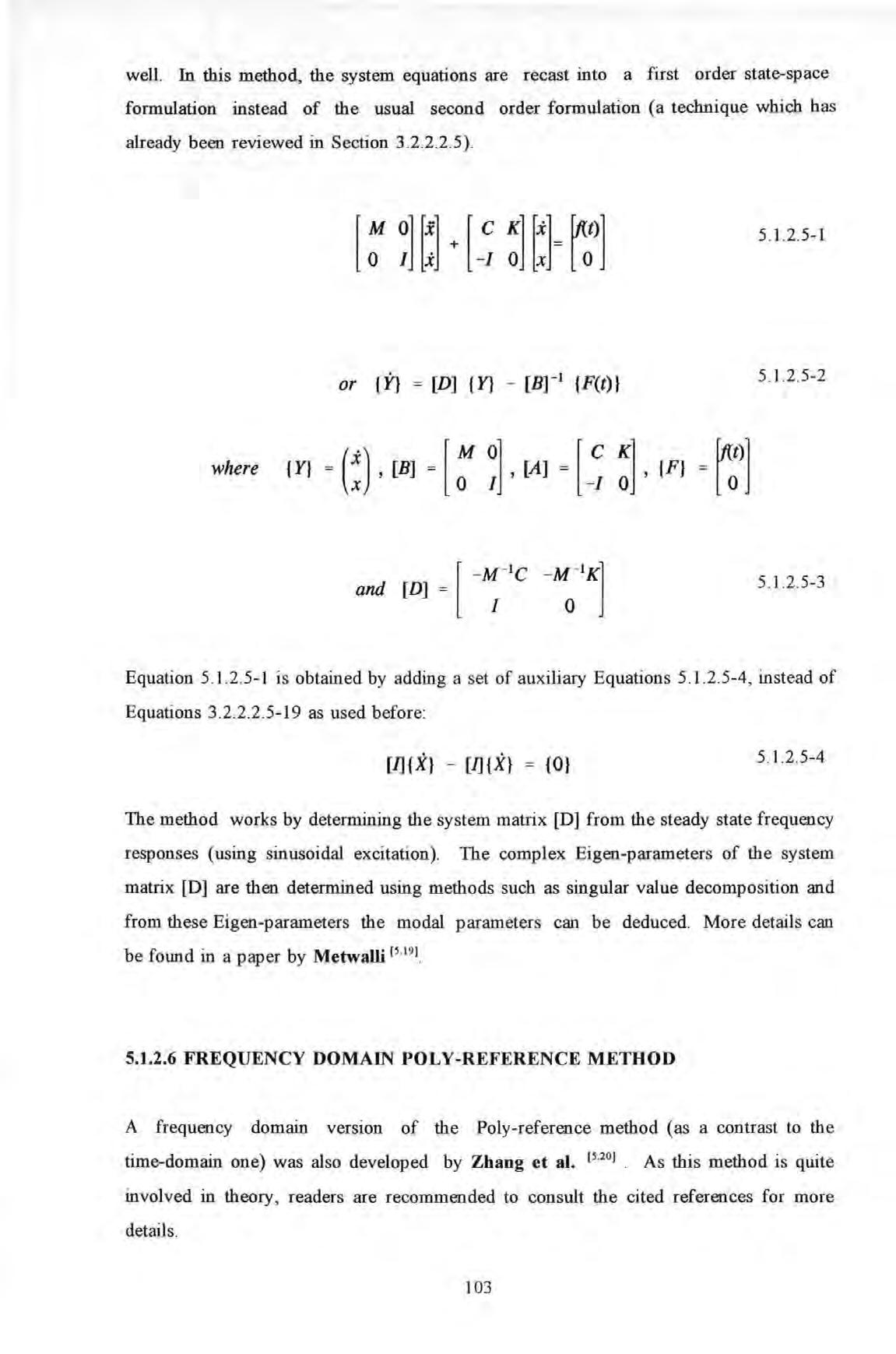
Equation 5 1.2.5-1 is obtained by adding a set of auxiliary Equations 5 1.2 5-4, instead of Equations 3 .2 .2.2 .5-19 as used before:
The method works by determining the system matrix [D) from the steady state frequency responses (using sinusoidal excitation). The complex Eigen-parameters of the system matrix [D] are then determined using methods such as singular value decomposition and from these Eigen-parameters the modal parameters can be deduced. More details can be found in a paper by Metwalli 15 191
5.1.2.6 FREQUENCY DOMAIN POLY -REFERENCE METHOD
A frequency domain verswn of the Poly-reference method (as a contrast to the time-domain one) was also developed by Zhang et al. 15 201 As this method is quite involved in theory , readers are recommended to consult the cited references for more details .
5 1.2 5-1 or (:YJ = [D] {Y} - [Br 1 {F(t)} 5 . 1.2 .5-2 where IYJ [B] :] ,IF} 5 1.2 5-3
[J]{X} - [IJ{X} = {0} 5. 1.2.5-4
I 03
5.1.3 SUMMARY
In summary, many of the methods described so far possess certain inherent strengths as well as weakness. The appropriateness of a method depends mainly on the particular situations encountered. Some methods work well in some situations but worse in others Therefore no single method can be a panacea for aJI situations

The brief review has highlighted the often conflicting requirements between the simple and the sophisticated methods, such as :
a . the quantity and quality of data required ,
b the accuracy achieved ,
c the efficiency of use,
d the computational requirement etc
Simple SDOF methods are intuitive to use but slow in operation and require a lot of interaction from an analyst. They are also les s accurate unless remedial measures to account for the residual effects have been taken In contrast, most MDOF methods can be programmed to run almost automatically once the initial estimates have been given to start the process Because very little interaction is demanded from the analyst , these methods are extremely fast and efficient to analyzed a large set of data . Above all, th e MDOF methods are capabl e of providing a consistent set of modal parameters for th e complete set of data for all the test positions . Whereas this is difficult for SDOF methods to do For the very same reason , these methods are also sensitive to discrepancy and inconsistency caused by measurement errors.
MDOF methods requue computers with large memory capacity and high speed of computation for performing the large scale data processing involved . With the advent of computer technology, these requirements which a main frame barely meet a decade or two ago can now be fulfilled by a personal computer.
104
5.2.1 BACKGROUND
In general , experimental data obtained from fie ld tests are of inferior quality than their laboratory counterparts Field d ata are often noisy and have undesirable frequency reso lut ion because of the severe time constraints in taking measurements . Global MDOF methods are thought to be unsuitable becau se the quality of the field data may not be good en ough to be a consistent set.
The alternative algorithm developed during the course of this work is a direct least-square fitting method The simplicity of the algorithm makes the curve-fitting process more apparent to the lay users and this is considered to be a di s tinct advantage. By performing the pre-treatment of data (as explained in Section 5 . 1. 1.2 ) as a pre-requisite step, the algorithm can yield accuracy comparable with other accurate methods. However the algorithm is never meant to compete on these g round s The algorithm has a few features common with the linear regres s ion method which , to most people, is a very familiar mathematical technique Hence, users can find it comfortable to use In lin e with most SDOF methods in its class, this algorithm is al so based on the usual single-mod e assumption . The method has the following characteri stics (some of these are common to other SDOF methods as well and a re not neces sarily unique to this method) :
1 This algorithm does not rely on any geometri cal forms : circles , straight lines or others , explicitly as a curve-fitting criterion.
2 This algorithm is computationa ll y very si mple, intuitive to use and can be easily implemented in a spread sheet or simp l e hand-held calculator application.
3 . This algorithm does not require the manipulations of large matrices.
4 . No initial estimate i s required to start the calculation process .
5. The determination of dampin g parameters i s totally independent of the other

5.2
THIS
THE METHOD USED IN
INVESTIGATION
105
modal parameters so errors in determining one parameter will not accumulated in determining the next one
5.2.2 DEVELOPMENT OF THE ALGORITHM
A stepwise development of the a lgorithm will be given in this section . It starts with the familiar equations of motion of a reduced order dynamic system under harmonic excitation :
and {F} are respectively the Fourier Transforms of displacement {x(t)} and force vectors {f(t)} and are functions of angular frequency ro
which can be obtained by applying Fourier Tran sform to Equation 3 2 2 2 1- 28 Using the linear transformation between spatial and natural (or modal) coordinates using the undamped modal matrix [ <1>] (which is real) :
2 2-1) becomes :
Pre-multiplying Equation 5 2 2-3 by [ <1> f to obtain :
From Section 3 2 2 2.4 concerning orthogonality , the matrix triple products depicted in Equation 5 .2 .2-5a and 5 .2 .2-5b are known to yield the diagonal modal (or sometimes known as Generalised) mass and stiffness matrices (which again are all real) :

where ( -w 2 [M] + j w [C] + [K] ) {X(w)} = {F(w)} (522- 1) {X}
{ X(w) l = [Cl>] * I 11 (w) } (52.2- 2)
(5
( - w 2 [M] [Cl>] + j w [ C] [Cl>] + [ K] [Cl>] ) { 11 ( w) } = {F( w)} (5 2 2-3)
Hence Equation
(5 2
2-4)
106
If proportional damping is assumed, then (C) can be diagonalised by the undamped modal matrix in the way as stipu lated in Equation 5 .2 .2-5c :
where [C*] is the diagonal modaJ or generalised damping matrix .
The modaJ force vector ts gtven as :
In effect, Equation (5.2 2-6) represent a set of uncoupled equations of motion since the modal mass, stiffness and damping matrices are all diagonal matrices The matrix
Equation (5 2.2-6) can be re-written as a set of scalar equations for each mode : (5.2.2-7)

where i = 1, 2, 3 .... so on and refers to the mode No.
Within a narrow frequency band close to roi , if the response X , at nodal point s is pre-dominantly contributed by the ith mode, i e residuaJ effect from out-of-range modes is
[ M* ] = [ <b f [M] [ ] (5.22-5a) [ K* ] = [ f [.K] [ ] (52.2-5b)
[ c. ] = [ f [ C] [ ] (5.2.2-5c)
{ F* } = [ f { F } (5.2.2 - 5d) hence ( - w 2 [M*] + j w [ C*] + [K*] ) {fl (w) } {F*(w)} (5.2.2-6)
N xs = E [ <t> si ,i J i = l
smce
(5.2.2-8)
107
neglected, then :
and if there is only one excitation force
if receptance a is defmed as :
K '; and C'; can be obtained similarly by dividing K.; and c·; with respectively .
Notice that all M'; , K ; and c·; (called effective mass , stiffness and dampin g) are assumed
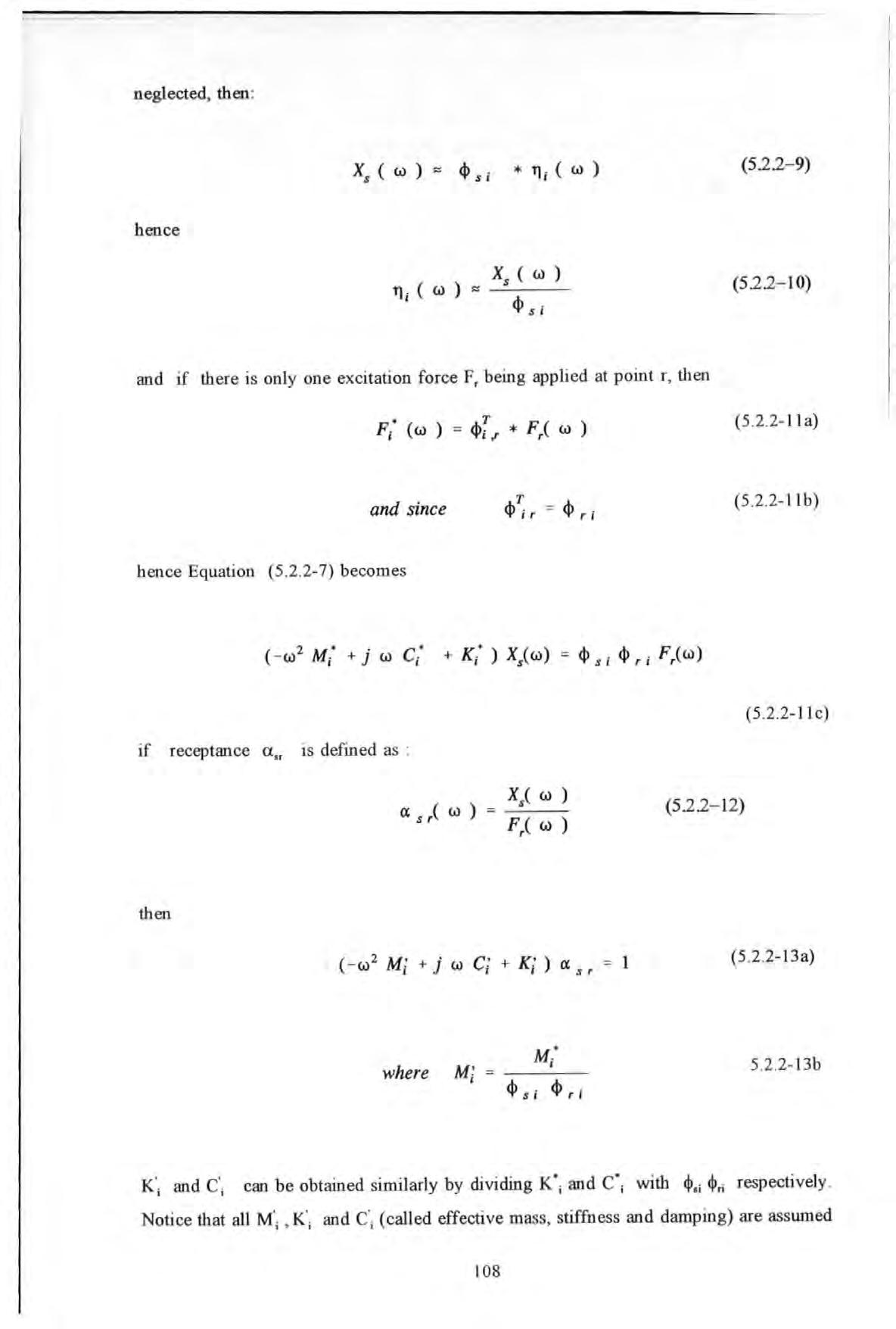
xs ( w ) ::: <I> s ; * TJ; ( w ) (522-9) hence TJ; ( w ) ::: xs ( w ) (52.2- 10) <I> s i
F.
r ,
(5 .2 .2- lla) and since (5 2 2- llb) hence Eq uation (5 .2.2-7) b ecomes (5 2 2- 11c)
being applied at point
then
(5.2.2 - 12)
( - w 2 Mi + j W Ci + Ki ) a s r = 1 (5.2 .2-l3a) where 5.2.2-13b
then
108
real . Also since a is a complex quantity and so is its reciprocal (called dynamic stiffness) : (522-14)
where
(5 2 2-15a)
(5 .2.2-15b)
in which 91 and 3 stand for the real and imaginary parts of receptance respectively . A note of caution must be made here because of the assumption made in arriving at Equation
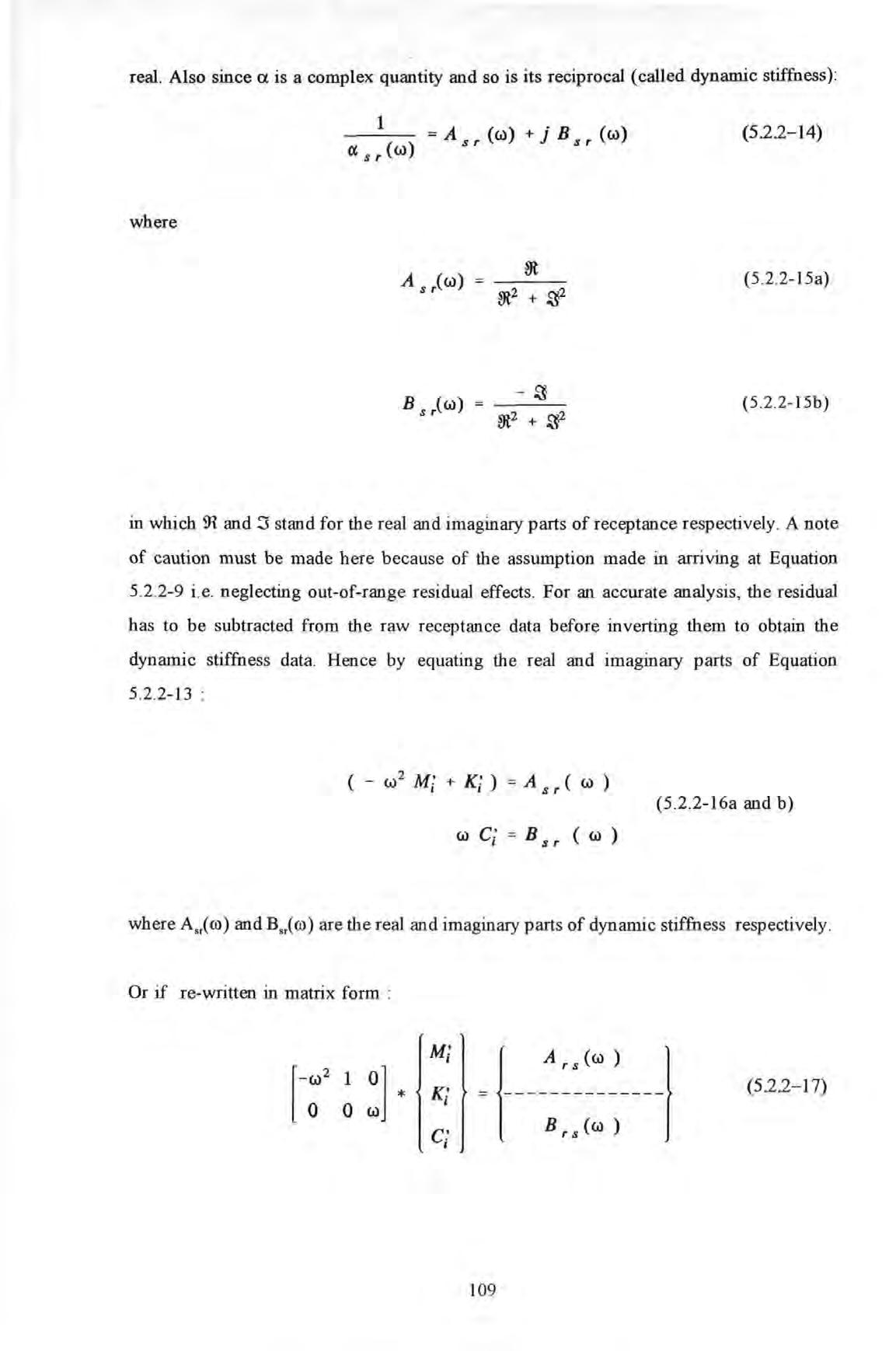
5 2 2- 9 i e neglecting out-of-range residual effects For an accurate analysis, the residual has to be subtracted from the raw receptance data before inverting them to obtain the dynamic stiffness data Hence by equating the real and imaginary parts of Equation
5 2 2-13 :
where A.,(ro) and B,.(ro) are the r eal and imaginary parts of dynamic stiffness respectively .
Or if re-written in matrix form :
( - w z Mi + Ki ) = A s r ( w ) (5 .2 .2-16a and b)
= B (w) 1 s r
wC:
K.' I c: I l A r s (w ) I = - -B r s (w ) (5 22-17) 109
for n different frequencies close to the ith undamped natural frequency :
If the ith mode is considered dominant within this range of frequencies, then each of these frequencies provide a set of equations, similar in form to Equation 5 2 2-17 :
which is of the standard form of mo st system of linear eq uation s.
The dimension of the coefficient matrix [A] is 2n X 3 Since the number of unknowns in this case is only 3, hence a minimum of 3 equations is sufficient for a so lution The solution obtained by using more than this statutory mmunum IS called the pseudo-inverse solution which can be obtained by an application of the following equation
Equation 5 2 2-20 provides an Wlbiased estimate of unknown vector {x} So as the number of frequency points used in the curve-fittin g process increase so does the size of [A]. However it can be shown that the following matrix multiplications can be redu ced to very simple forms :
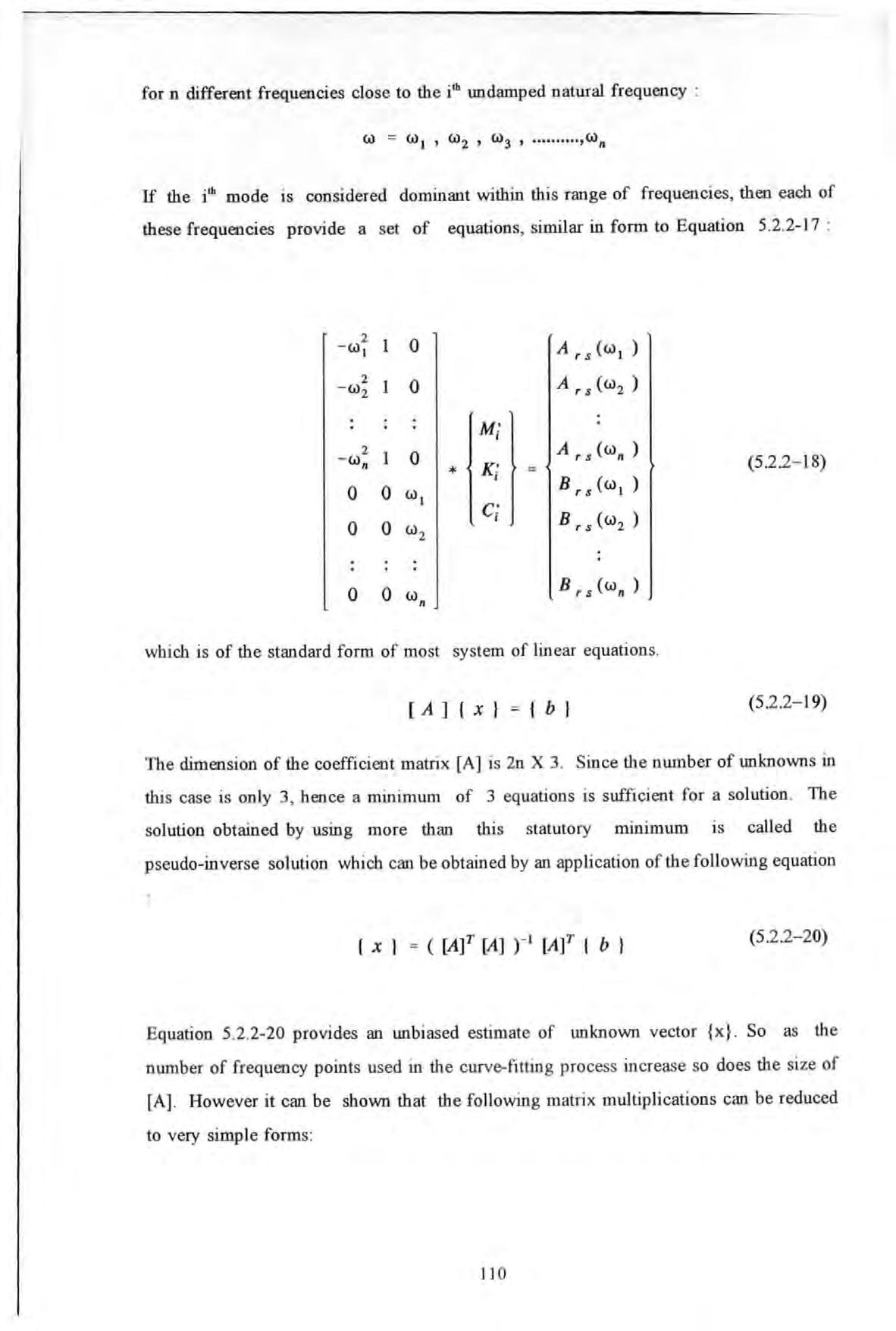
w = w 1 , w2 , w3 , ,wn
2 1 0 A,.s(w 1 ) -w. 2 1 0 A r .s (w2 ) -w2 I 2 1 0 A, 3 (Wn) - wn * I B r .s (W 1 ) 0 0 w. c: B r .s (w2 ) 0 0 I w2 (5.2.2- 18) 0 0 wn B,.s(wn)
[A]{x} =
(5.2.2-19)
{b}
t x 1 = c[Af [AJ r• [Af t b 1 (5.2.2-20)
110
which is only a 3 X 3 matrix Similarly, it can also be shown that :
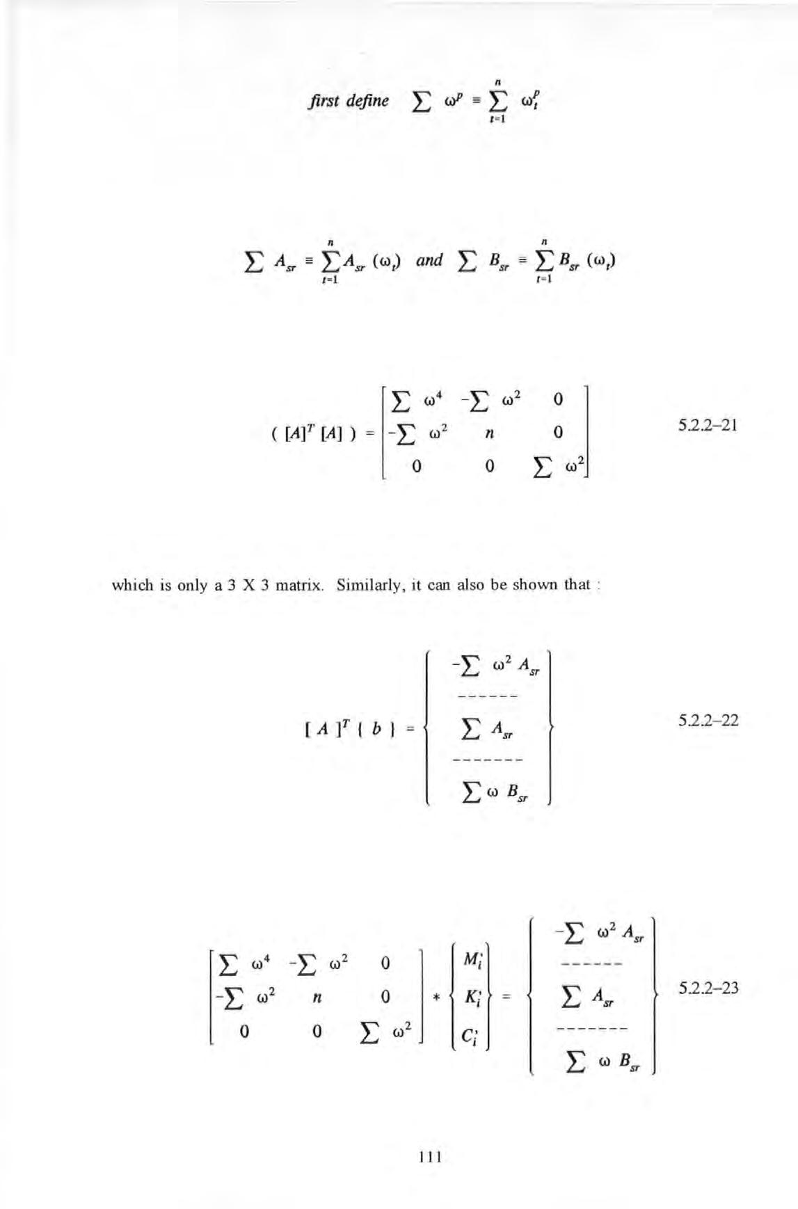
n first define .E wP = .E (J)f t • l n n L AST = .EAsr ((J)t) and L 8 sr = L Bsr ((J)t) t =l t =l .E (J)4 _ E (J)2 ( [Af [A] ) = - L (J) 2 n 0 0 0 0 .E (J)2
[A f { b } -E (J)2 Asr .E (J)4 -E (J)2 0 M : I-I: (J)2 n 0 * K: LAST I 0 0 I: (J)2 c.· ------I E (J) Bsr I I I 52.2-21 522-22 522-23
If data were accelerance (or inertance), revised form ul ae would have to be used The conversion from receptance to accel erance is quite straight forward :
where accelerance Yri ro ) is similarly defined as receptance except that acceleration now replaces displacement. Similar to Equation 5 .2 .2-14 , the reciprocal of accelerance is defined as :
where A.r and B·,r are simi l arly defined as their A,r and B.r counterparts as the real and imaginary parts of the inverse of accelerance It can be shown that the following equations can be derived:
The solution of the system of equations 5 .2 .2- 23 (of order 3) provide explicit express ions for the three unknowns :
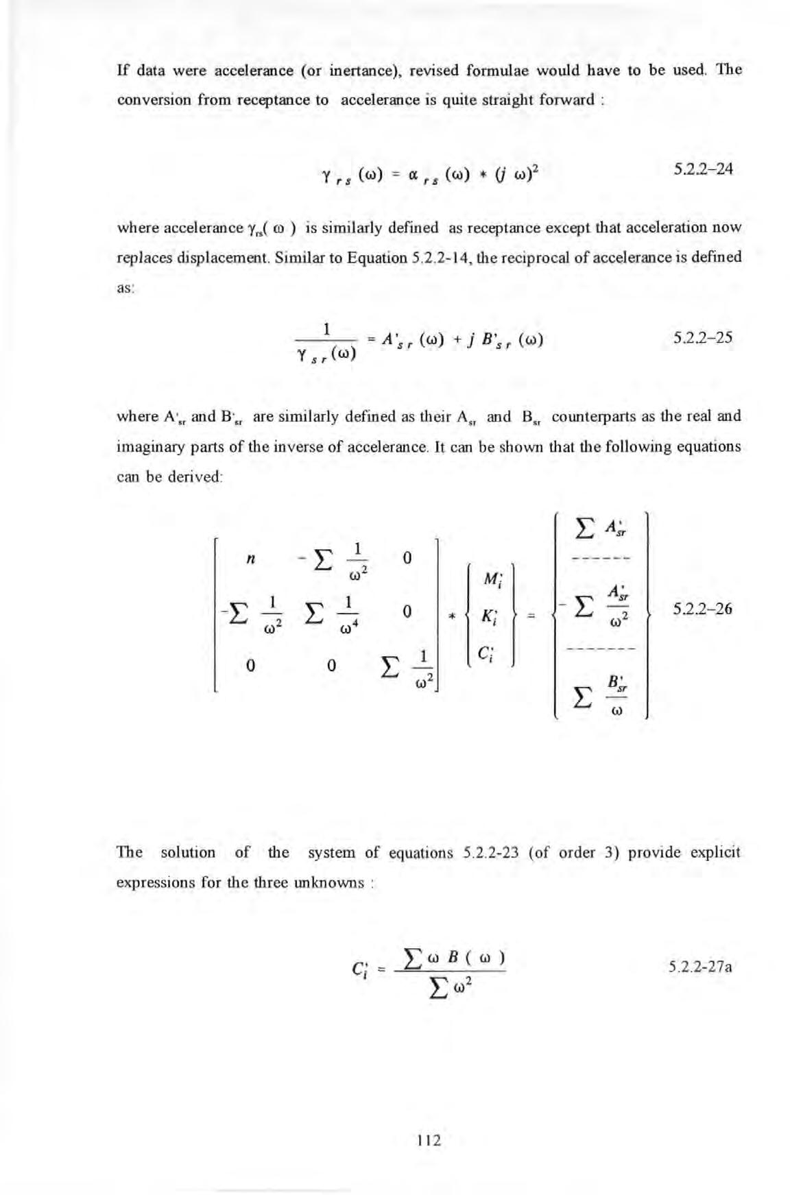
y r s ( w) = a r s ( w) * (j w )2 522-24
1 = A 's r ( W) + j B 's r ( W) Y s r (w) 5.22- 25
L A_;, -.E 1 0 n w2 I A' 1 1 - .E sr -.E .E 0 - 5.2.2-26 * w2 w2 w4 I 1 c 0 0 .E I w2 B' .E sr w
C= I 5 .2.2-27a 112
To obtain the various modaJ parameters, the followin g formulae can be us ed :
ffi; , and G.r.i are r es p e ctiv ely th e und amp ed n atura l fr e quency, modal damping factor and modal con stants of th e i'h mod e
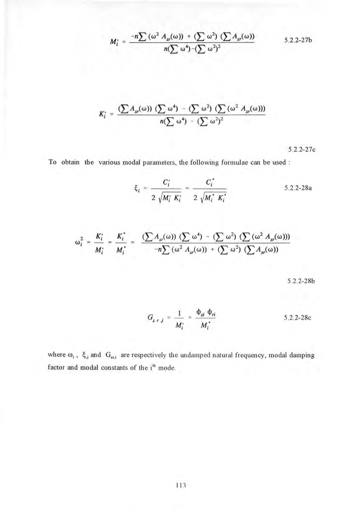
(LAs,(w)) (L w 4) - (L w2) (L (w 2 As,(w))) n(.L w4) - c_L w2) 2 5.2 2-27b 5 2 2- 27c
2 K! I I W; = - =M.* I I c I c: I 5 .2 .2-28a 2 JM: K' I I (LA s,(w)) (L w 4 ) - (L w 2 ) CL (w 2 Asr(w))) -ni: (w 2 As,(w)) + (L w 2 ) (LAsr(w)) 5 2 2-28b Gs r ; = 1 _ <Psi <l>,; ' M : I I 5 .2 .2- 2 8c where
11 3
5.3 IMPLEMENTATION AND VERIFICATION

The algorithm was implemented in a numb er of computing environments and platforms :
Hewlett Packard HP Basic® Version 4
MA TLAB ® routines and spread sh eet application in QUA TIRO PRO®.
The mechanics (not accuracy since values a re roWlded off to fit in the t ab l e) of the calculation at work can be illustr ated by the following example (usin g the synthesi zed data of the four-mode fictitious system to be described below) :
11 4
TABLE 5.3-1 TABLE ILLUSTRATING THE MECHANICS OF THE CALCULATION USING THE PROPOSED ALGORITHM
Using Equations 5.2 2- 27a to 5 2 2-27c in w hi ch onl y si mp le multiplications an d divisions are involved , the modal parameters calcul at ed are :

171317 0.072 -55.00 -1888 42.20
undamp ed natur al 25 25 18 frequency (Hz) damp ing factor 0 01 0 0076 m odal constant (kg- 1 ) 1.0 0 745 11 5
ASSUMED CALCULATED VALUES VALUES
The discrepancy is due to rounding errors in the initial input data (accelerance values etc) and in performing the calculation . Also it is due to the fact that removal of residual effect from the data has not been performed .
Commercial spread sheet programs such as QUA TIRO PRO® are best suited to perform these 'mechanical' row- and column-wise calculations . The program , which was written in Matlab® and run under Microsoft Window00 3 . 1, provided a very efficient interactive environment for performing the analysi s reported here
The computational procedure was verified based on computer simulations subjected to a number of scenarios. The data were synthesized from a fictitious 4-modes vibration system , with relatively well separated mode s and known modal parameters. Hence the accuracies of this method can be quantified readily by comparing the results with their known values .
The various scenarios are intended to st udy the combined effects of the levels of damping and frequency resolutions on accuracy The levels of damping assumed were ranged from 001% to I 0% of critical damping values TI1ese values covered from light to the heavily damped situations The frequency resolutions of data were 0 1, 0 5 , 1 0 and 2 5 Hz The effects of random noise on sensitivity of the method have not been investigated because data deliberately polluted with artificial Gauss ian type random noises may not be entirely representative of those encountered in practice .
The modal parameters assumed for the fictitious system are summarised and tabulated in Table 5 .3-2 .

11 6
In addition to comparing each of the individ ual assumed and determined modal parameters, a statistic called quality-of-fit factor QF is used to indicate q uantitatively how good or bad the overall quality-of-fit or accuracy is . TI1is QF factor has been defined in Section 6 2 3.2 and is subjected to the same limitations in its interpretation as stated there.

The effects of the selection of the frequency data points, in terms of their numbers and positions , have no t been thoroughly investigated. However as a general rule, the use of a smal l number of points will yield good results When choosing a l arge number of points for fitting , unless all the points are weU within the resonant region, this action will be counter-productive and will yield bad results as the underlying assumptions are more likely to have been violated .
Although the analysis method ts based on SDOF assumption , the effects of neighbouring modes (called m odal interference) can be taken care of by subtracting the
TA BLE 5 3 -2 ASS UMED M O DAL P ARAMETERS F OR A F OUR-MODES F I CTITIOUS SYSTEM
MODAL PARAMETERS FO R
ODES FICTITIO
SYSTEM UNDAMPED NATURAL MODAL CONSTANTS RANGE OF DAMPING FREQUENCY VALUES Hz kg-1 I %OF CRITICAL D AMPING 25 1.0 I .001 T O 10 50 2.0 .001 TO 10 65 2 0 001 TO 10 80 0 5 001 TO 10
ASSUMED
A FOUR-M
US
I 17
effects of these modes from the analyzed mode. Hence accuracy can be further improved by repeating these subtraction procedures in an iterative fashion
The case of 10 % of critical damping has been chosen as an illustration . Although the modal frequencies are relatively well spaced apart, the higher damping level causes considerable 'interference' in the FRF . Analysis conducted using mode s ubtraction on the first three modes has shown some improvements over tho se analysis without using mode subtraction .
For the sake of easy explanation , an indicial notation M(r,s) was devi sed and defined to illustrate the mode subtraction operations carried out as fo ll ows :

where r is the mode number
s is the number of iterative cycles performed
For instance, M(3 ,2 ) = M(3 , 1) - M(2 , l) means that the results for mode number 3 after two iterations is obtained by s ubtractin g the effects of mode number 2 (from the first iteration) from those of mode number 3 (after the f irst iterations). Table 5 3-2 summarizes the results of analy sis as follows :
11 8
TABLE 5 .3-3 RESULTS OF MODAL PARAMETERS DETERMINATION USING ITERATIVE MODE SUBTRACTION FOR THE FOUR-MODE FICTITIOUS SYSTEM
RESULTS OF MODAL PARAMETERS DETERMINATION USING ITERATIVE MODE SUBTRACTION FOR TIIE FOUR-MODE FICTITIO US SYSTEM

MODE NO
RESONANT FREQUENCY Hz MODAL CONSTANT 11 9 DAMPING FACTORS RESULT FROM
TABLE 5.3-4 EFFECTS ON QF FACTORS BY USING VARIOUS MODE COMBINATIONS

EFFECTS ON QF FACTORS BY USING VARIOUS MODE COMBINATIONS
Table 5.3
shows the consistent improvement in QF values from .474 to .951 after a few iterations .
The running of the program in action and the graphical results obtained are briefly described below. Figure 5.3- 1 shows a typical accelerance (or inertance) FRF of the fictitious system . The suspected resonant peaks in both the modulus and imaginary plots are first marked with vertical lines using a screen cursor.
MODE COMBINATIONS QF FACTORS IMPROVEMENT OVER PREVIOUS RUN M(I ,0) + M(2 ,0) + M(3,0) .474 NIA M(l ,O) + M(2 ,0) + M(3 , 1) 807 YES M(l ,O) + M(2 , 1) + M(3 , 1) 854 YES M(l , l) + M(2 , 1) + M(3,1) .951 YES M(l , l) + M(2 , 1) + M(3 ,2) .937 NO
-4
120
After responding to a series of requested inputs by the program with regards to : the number of points neighbouring each of the marked peaks used for curve-fitting , whether or not mode subtraction is required,
computation then proceeds using the proposed algorithm . To appraise the results obtained, overlaid plots of the original and the so-called regenerated FRF curves are displayed for visual inspection by the analyst. The regenerated FRF curves are plotted based on the determined modal parameters determined (Note the full set of the modal parameters results determined in the simulation experiment are tabulated in Appendix 5.4). A selective sample of these results (plots) for the various conditions studied was shown in Figures 5 .3-2 to 5 .38.

10• 10• j 10-1 100 200 100 200 300 400 1500 data paint. 1100 700 n. band•LJ!._•alc:• u•1na cu,..o,... ftl• d3 300 400 1500 1100 700 data paint. QOO eoo QOO 1000
Figure 5 3-1 Marking of resonant peaks with vertical lines on the modulus and imaginary Inertance FRF plots
10 20 30 40 eo eo 70 eo ao 100 .,,.•quency In ha
12 1
Figure 5 3-2 Overlaid plots of original and regenerated Inertance FRF for the fictitious system with frequency resolution of 0. 1 Hz and damping factor 0.1 % of critical damping .
Figure 5 3-2 sho ws that for a frequency resolution of 0 1 Hz and light damping (0 1% of critical damping), the correlation between the two curves in both the modulus and phase plots are very good

Figure
Overlaid plots of original and regenerated Inert.ance FRF for the fictitious system with frequency resolution of 0 . 1 Hz and damping factor 1 % of critical damping
With 1% damping and the same resolution of 0 1 Hz, the correlation of the curves shown in Figure 5 .3-3 . is not as good as that shown by Figure 5 .3-2 .
Figure 5
Overlaid plots of original and regenerated Inertance FRF for the fictitious system with frequency resolution of 1 Hz and damping factor 0.001 % of criti cal damping
10 20 30 40 l50 ISO 70 eo 90 100 10 20 30 40 50 eo 70 eo QO 100
5 .3-3
I]: I ::CM:; 10 20 30 40 50 eo 7o eo 80 100 1r•qu•ncy In nx 10 20 30 40 50 ISO 70 eo 80 'frequency In hz
122
3-4
% of critical damping.
show that for a frequency resolution of 1 Hz and a range of damping (ranged between .00 I% to O.I% ), correlation is consistently worst at those regions near resonances and anti-resonances where phases change abruptly because of the lack of frequency resolution
Figures

.,,.•qu•nay In hx 10 20 30 40 50 eo 70 eo QO 100 'fr.qu•nay In ha
10 20 30 40 eo eo 70 eo QO 100 10 20 30 40 eo eo 70 eo QO 100
Figure 5 3-5 Overlaid plots of original and regenerated Inertance FRF for the fictitious system with frequency resolution of I Hz and dampin g factor OI % of critical damping
Figure 5 3-6 Overlaid plots of original and regenerated Inertance FRF for the fictitious system with frequency resolution of I Hz and damping factor 0 1
123
5 3-4 to 5.3-6
Figure 5 3-7
Overlaid p lots of original and regenerated Inertance FRF fictitious system (with frequency resolution of 2 5 Hz and damping factor 0 001 % of criti cal damping
With a even coarser resolution at 2 .5 Hz, Figure 5.3-7 shows that even with the lightest damping , the correlation deteriorates badly . Results tabulated in Appendix 5.4 show that the errors on the modal parameters set determined are all significantly higher than that of the finer resolution cases given the same damping factors

Figure 5 3-8
Overlaid plots of original and regen erated Inertance FRF for the fictitious system with frequency resolution of 2 5 Hz and damping factor 10 % of critical damping
Figure 5 3- 8 shows the worst scenario (i e heavy damping plus coarse resolution) amongst the conditions studied here Results tabulated in Appendi x 5.4 show that for mode 1 to 3, the errors can be as much as 50% or more in these circumstances
f,..equanc:y In ha .,0 20 30 <4-0 150 eo 70 eo GO 100
•o:t ' : : : J 10 20 3o 40 so eo 7o eo Go 100 'fr"equ•"oy In ha
t
124
5.4 COMPARISON OF THE PROPOSED WITH SOME CONVENTIONAL METHODS
There are a number of similarities between the proposed method and the dynamic stiffness method which are worthy of taking note First of all , the proposed method requires the formulation of equation in the following ways : 1 (5.4-1) as r
Or in the case of h ysteretic damping , the damping term m Equation 5.4-1 is adjusted according}y : 1 (5.4- 2) as r

the usual formulation in dynamic stiffness method is of the form :
Equation s 5.4-1 and 5.4-2 are linear with unknown constants s uch as : M';, C'; and K'; Using dynamic stiffness methodology , the plot of the real part of dynamic stiffness data against ro 2 will produce a straight lin e with a slope equals to - M '; , and intercept on the vertical axis K'i. Similarly, the plot of the imaginary part of dynamic stiffness data against ro will also be a straight line with a s lope equals to c'; . In the hysteretic damping case, the plot of the imaginary parts of dynamic stiffness against ro should also be a straight line with zero slope (i.e. it is independent of frequency ro) and the intercept on the vertical axis equals to a constant (equal to Y; K ';) .
Whereas based on the Eq uation 5.4-3, the plot of the real part of dynamic stiffness against ro 2 will produce a straight line with a slope equals to ( - 1/G,,.; ) and the plot of the imaginary part of dynamic stiffness against ro will also be a straight line with zero slope and the intercept on th e vertical axis equals ( Y ; ro; 2/G.,,; ) .
1 2 1 2 1 + U) i ( -) + J 'Y i U) i ( - ) G sr,j Gsr,i 5.4-3
125
Secondly, both the proposed method and the dynamic stiffness method require the removal of the residual effect of out-of-range modes from the raw data as a separate and a prerequisite step for an accurate analysis. Thirdly, both the proposed method and the dynamic stiffness method assume real modes hence they all implicitly assume proportional damping.

However, despite these similarities, the two approaches do differ in· the fundamental thinking. The proposed method here determine the spatial parameters M; , K"; and c·; (called effective mass, damping and stiffness) directly. This approach is in line with the philosophy as will be discussed in Chapter 6. From these spatial parameters, the modal parameters are then derived as 'by-products'. Whereas the dynamic stiffness method determines the modal parameters directly. Unlike modal parameters, these spatial parameters still retain some quantitative descriptions of mass, stiffness and damping of a system.
A comparison of the proposed algorithm with two other SDOF methods (i.e. the circleand Dobson's improved straight-line-fit methods) was carried out. Again the same 4-modes fictitious system was used for this study. It was expected that the proposed method would achieve similar accuracy as the corresponding dynamic stiffness method would if the residual-removal step was carried out as a pre-requisite step before fitting,. The intention of this comparison study was to determine the accuracy of the proposed method in the event that the residual-removal step was not carried out. The areas of comparison were also concentrated on the effects of different levels of damping, frequency resolutions and fitting data points selections on accuracy. The results obtained from the three methods carried out are tabulated in Appendix 5.4 but some general observations are summarised below.
In general the circle-fit method is not suitable for very light damping cases and can produce large errors if frequency resolution is not fme enough. In the heavy damping situations, this method has yielded results with better accuracy.
The Dobson method has a good overall performance in many situations due to the elaborate procedures included in the program:
a. to subtract or minimize the effects of modal'interference' from neighbouring modes on the analyzed mode.
126
b. to account for complex residual effects from out-of-range modes.
In the case of the author's method, it can still produce acceptable results with reasonable accuracy in the cases of good frequency resolution and low damping. For instance, in the cases of 1% critical damping and a frequency resolution of 0.1 Hz (these are similar to the situations encountered in the Fire Tower tests as described in Chapter 8), the author's method produces errors of no more than 5 % and in most cases less than I % in the case of modal constants. However in the cases of undamped natural frequencies and the damping factors, these are quite accurately determined as shown in Table 5.4-l which is an extract from the more thoroughly reported results given in Appendix 5.4.
TABLE 5.4-l PERCENTAGE ERRORS IN THE MODAL PARAMETERS DETERMINED USING AUTHOR'S METHOD
Hence a small sacrifice in accuracy may be a justifiable price to pay if simplicity and speed are desired. The column-wise operation as shown in Table 5.3-1 when implemented in spread sheet application is a very intuitive medium in which to see and learn the curvefitting at work.

WITHOUT MODE WITH MODE SUBTRACTION SUBTRACTION %ERRORS IN %ERRORS IN UNDAMPED MODAL DAMPING UNDAMPED MODAL DAMPING NATURAL CONSTANT FACTOR NATURAL CONSTANT FACTOR FREQUENCY FREQUENCY MODEl 0 1.99 .02 0 1.7 .02 MODE2 0 .33 .01 0 .01 .01 MODE3 0 .27 .01 0 .002 .001 MODE4 0 2.1 .3 0 4.42 .05
127
5.5 CONCLUSIONS
The proposed algorithm is an acceptable approximation tool for the determination of modal parameters. It works rather well if the modes are well separated, damping is light and frequency resolution is adequate. However, the built-in assumptions, such as: proportional damping and hence real modal constants etc, have to be borne in mind when applying the algorithm. For an accurate analysis, pre-treatment of raw receptance data is required to remove the residual effects before carrying out the curve-fitting.

128
CHAPTER 6
EXTRACTION OF SPATIAL PARAMETERS FROM FORCED VIBRATION DATA

6.0 INTRODUCTION
This chapter will first review a number of conventional (modal) methods in Section 6.1. An alternative non-modal (spatial) method developed by the author is presented in some details in Section 6.2. The background theory is covered in Section 6.2.1 and the steps in its derivation are described in Section 6.2.2. The computer simulation used to validate the method was reported in Section 6.2.3. The applications of this method to data obtained from a number of real structures are presented in Section 6.2.4. A general discussion of the method is presented in Section 6.3. Finally, the conclusions are stated in Section 6.4.
The exact origin of the use of the terms spatial parameter and spatial model is not known. It is believed, however, that it is probably attributed to the work published by Gleeson 16 11 in 1980 which was entitled 'Identification Of Spatial Models'. The spatial parameters here follow closely with Gleeson's defmitions i.e. they refer to the mass, stiffness and damping matrices which, in physical terms, represent the inertial, elastic and energy dissipating properties of a structure.
The attempt to Derive Spatial Parameters from Experimental Data (DSPED) is not new.
In fact, the history went back as far as the 1960's. Broadly speaking, these methods share a lot in common but also differ from each other in a number of respects such as:
129
a. whether pnor knowledge of or assumptions about some of the matrices are required,

b. whether the approach is a direct one or is one based on iterative search or optimization methodology and
c. whether the identification of modal parameters are required prior to the determination of the spatial matrices.
For the sake of brevity, some important concepts and terminologies which are frequently referred to in the text are first defined. A structural model is often classified as low-order, high-order, complete or in-complete. This classification IS based on the relative magnitudes of the three non-negative integer quantities :
N : the total number of feasible DOF (or modes) of a structure,
n : measured DOF's in forced vibration tests and
r : the number of resonant modes within the frequency band of analysis.
Apart from fictitious ones, most real-life structures are continuous rather than discrete by nature. Therefore these structures should possess inherently infmite degrees of freedom or modes i.e. N is infmite. The natural frequencies corresponding to these modes are distributed over a wide frequency band. However some structures can often be classified as a SDOF or a MDOF (single- or multi- degree-of-freedom) system, where the degrees-of-freedom N is usually a small integer. Such a fmite DOF system can exists because only a small number of possible DOF's is enough for defming its deformation field. This may be achieved by the ways the system is configured and constructed that the continuous system can be approximated as a fmite DOF lumped system.
Closed-form analysis of complex continuous structures is seldom carried out because of the mathematical difficulty involved. This statement remains true with the exceptions of some of the simplest structures only i.e. a beam, a rod etc. Hence analysis are often pursued by approximation methods. Finite Elements (FE) and Boundary
130
Elements (BE) methods are the two most popular methods used by analysts. An FE or BE model of a structure usually incorporates a finite number, but still a very large number, of nodes and elements. The deformation field of each element is specified by the DOFs at all its nodes. Hence the total number of DOFs of all the active nodes and elements N is frequently very large. For this reason, an FE or a BE model is often classified as a high-order model.
By contrast, only a relatively small number of DOF can be measured from experiment. Therefore n is usually much smaller than N. For this reason, a model synthesized directly from measured data is often classified as a low-order, condensed or spatially trnncated model.
Apart from spatial truncations, most practical models are also modally or spectrally truncated. This is because, in practice, only a small number of modes in a very narrow frequency band is determined experimentally. As a result, r is usually much smaller than n. The model so obtained is called an incomplete model. Otherwise, if r is equal to n then the model is called a complete model.
6.1 CONVENTIONAL MODAL METHODS
By defmition, most of these methods require the determination of the relevant modal parameters as a pre-requisite step before the spatial matrices are determined.

6.1.1 AN OVERVIEW OF THE HISTORICAL DEVELOPMENT
The most notable contributions in this field can be traced back to the US National Astronautical and Space Administration {NASA) research programme in the late 1960's and the early 1970's. This programme was commissioned to investigate the techniques of experimental determination of structural dynamic models for aerospace structures. The driving force behind this development was the need to obtain valid experimental models which could be used for response analysis, load prediction and validation of analytical models of existing or modified aerospace structures. This technique was seen as a soft option for the more expensive, time-consuming, hardware testing often done on a trial-and-error basis. A number of investigations conducted by Rodden l6.2l, Raney and
131
Hewlett 16.31, Ross 16.41, Thoren 16.51, Young and On 16.61, Kozin 16. 71 , Berman and Wei J6.SI were either a direct or an indirect result of this programme.
Historically, DSPED have undergone different phases of change and development. It was first perceived by Rodden 16.21 in 1967 as a process of determining the structural influencing coefficients using ground vibration tests. In 1968, Kozin I6.7J considered this as a parameter identification process. The identification procedure which he proposed was based upon statistical expectations and time averaging technique. The method was tested by a series of simulation studies and proven applicable to both linear and non-linear systems.

Later m 1969, DSPED was perceived by Raney and Hewlett 16.JI as a process of determining a set of coefficients of the governing equations of motions of a structure formulated at the tested coordinates. These coefficients were effectively the elements of the mass, stiffness and damping matrices. This approach relied solely on the use of experimental near-resonance response data of a structure. Detailed knowledge of neither the structural nor material properties of a structure was required.
Young and On 16 61 summarized the vanous efforts and activities m this field and systematically categorized the various methods into five practical schemes. His work consolidated much of the thoughts and concepts associated with this technology.
In 1971, Ross 16 41 proposed a method which he described as a kind of synthesis technique. Two basic approaches were proposed: i.e. one of synthesizing low-order complete or incomplete models and the other of improving or updating existing high-order models. In particular to his approach, he proposed a novel normalisation procedure for the measured eigenvectors based on preserving the kinetic and strain energies of the real system. In 1972, Thoren J6.SJ reported similar efforts conducted in this area. He adopted a similar line of approach and applied his method to a real aerospace structural system. Some successes were claimed.
Since then, this activity was laid dormant for quite a while and relatively little literature on this subject was reported. However the recent up-surge of activities in experimental modal analysis has revived this activity again. Also because of the advance in computer software and hardware, the recently developed methods are increasingly geared
132
to large scale data processmg associated with high order models.
6.1.2 METHODS REQUIRING PRIORI ASSUMPTIONS
These methods are all typical m the way that priori assumptions on some of the parameters have to be made before other interested parameters can be determined. Nielsen rur is believed to be one of the first to have used this approach. He developed a number of procedures to calculate the elements in the stiffness and damping matrices from experimentally measured modal properties using classical normal mode theories.
In particular to his method, his procedures formulated the problem in such a way that the solution process was reduced to solving a system of simultaneous linear equations. The unknown vector in these equations contains the unknown elements of the stiffness and damping matrices. This method differs from the other methods based on optimization methodology in the way that the unknown parameters were determined directly rather than through iterative search schemes.
This procedure relied not only on a prior knowledge of the mass matrix but also on further restriction on the mass matrix for the procedures to work. In most cases, the mass matrix was assumed diagonal i.e. lumped mass rather than consistent mass model. With this method, the various requirements on the number of modes, hence the number of available equations, for a solution of a number of systems: known as simply-coupled, far-coupled and close-coupled systems, can be determined.
Sokal 16"91 proposed a similar approach which determined a stiffness matrix [K] directly from an assumed mass matrix [M] and an incomplete set of modal matrices. In particular to his approach, the algorithm proposed did not require the computation of the inverse of the modal matrix and was therefore applicable to incomplete models.
All these methods are based on the assumption that the mass of a structure can be estimated from design drawings with some degrees of certainty. However, m reality, the mass matrix [M] of a structure is not easy to determine accurately. These methods were applied to relatively simple systems only and spatial matrices of the low order category only were obtained.

133
6.1.3 METHODS USING ORTHOGONALITY PROPERTIES
These methods require a prior determination of a complete set of modal parameters which can be used to construct three square matrices: i.e. a diagonal spectral matrix [ro,1] (or a matrix of eigenvalues or square of natural frequencies), a diagonal matrix ro,] (here proportional damping is assumed) and a square modal matrix [<I>] (or a matrix of eigenvectors or modal vectors). Then calculation proceeds by using the orthogonality property of the vibration modes (real modes in the case of proportionally damped cases and generally complex modes for non-proportionally damped cases). This property can be stated mathematically with the following equations :
The matrices [ I ] is an identity matrix (i.e. modal vectors are normalised). ro,] and [ro,2] have previously been defined in Chapter 5. If the in verses of [<l>r 1 and [<I>rT exist, then the spatial matrices can be obtained using Equations 6.1.3-2: £Ml = £1llrr * £1llr' [Cl = £1llrr * * £1llr' [K] = £1llrr * [w 2l * £1llr'
Much of the works described previously in Section 6.1.1 have utilized this orthogonality property either implicity or explicitly. These equations can be used whether a low order or a high order model is concerned.
Using complex analysis, different formulations can be obtained. Potter and Richardson (6.UJ applied Laplace Transformation (denoted by the Si( ) operator) to the governing equation of motion to obtain a Transfer Matrix [T] which was defmed as the inverse of the system matrix as defined in Equation 6.1.3-5: 134
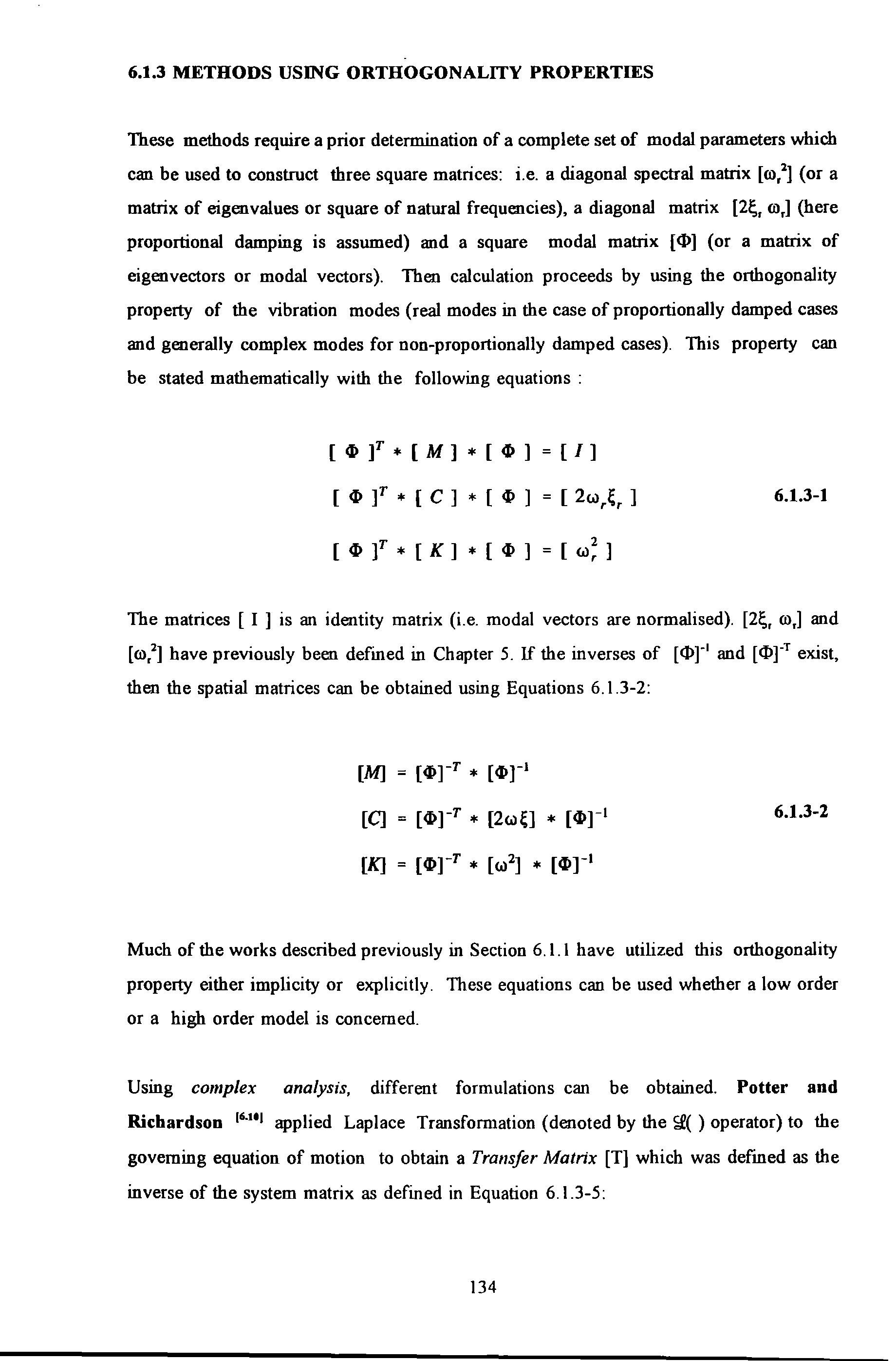
[lllf•[M] •[Ill] =[/] [ Ill f * [ C ] * [ Ill ] = [ 2w ] 6.1.3-1 [ Ill f * [ K ] * [ Ill ] = [ w; ]
6.1.3-2
Using this approach, expressions to obtain [M], [C] and [K] were derived in terms of the poles and the complex modal vectors of a system. So far the methods described in Sections 6.1.1 to 6.1.3 concern mostly with the determination of low order spatial matrices. These matrices though provide a valid mathematical description of a structure, their physical interpretation is sometimes difficult to obtain. Because the order of these matrices were condensed or truncated both spatially and modally to such a small number, in relation to the complexity of a structure, that the elements in these spatial matrices had lost their precise physical interpretation. A term by term comparison of these matrices with those of a high order FEM model was impossible. This is often the very reason why these methods have lost their appeal despite all other benefits they can offer.
6.1.4 METHODS USING OPTIMIZATION TECHNIQUES
Because of the drawbacks associated with low-order models, various investigators such as O'Callahan et al 16"11 ' 6. 121 , Barucb 16"131 adopted another approach utilizing computational optimisation techniques i.e. by correcting existing inaccurate spatial matrices of an FE model rather than synthesizing new ones. The corrected spatial matrices were obtained by imposing orthogonality criteria in the optimisation process. In operation, these methods required a set of approximate spatial matrices, called seeding matrices, as a starter prior to executing the correction procedures. The success of these methods
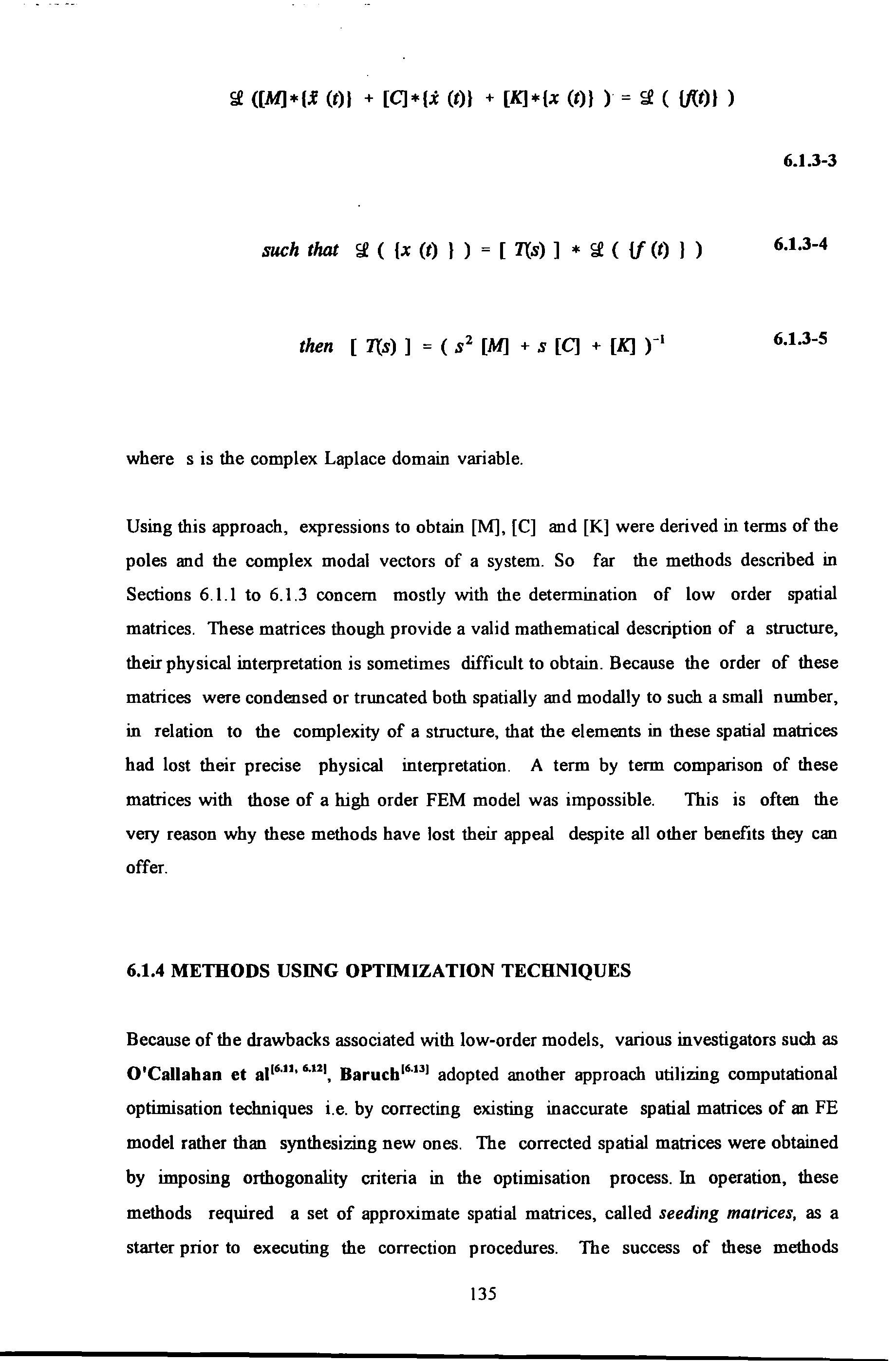
([M]* (.f (t)l + [C] * (i (t)} + [K] * (x (t)l ) = ( U{t)l ) 6.1.3-3 such that ( (x (t) } ) = [ T(s) ] * ( {f {t) ) ) 6.1.3-4 then [ T(s) ] = ( s 2 [M] + s [C] + [K] f 1 6.1.3-5
s
the complex Laplace domain variable.
where
is
135
often depended on how reasonably accurate the seeding matrices were m relation to their true counterparts. Otherwise, the iterative search might not converge to the true solution. So far, these methods have only been applied to analytical or academic type of problems. Successful applications to real systems are not reported.
6.1.5 SUMMARY OF MODAL METHODS
On the whole, all the methods discussed so far, are subjected to certain limitations in relation to their basic approach. In the case of synthesizing low-order models from a complete set of modes, the synthesis is a straight forward application of Equations
6.1.3-2. For the case of an incomplete set of modes, a direct use of these equations is impossible without proper pre-treatment. Because in practice, the number of measured DOFs p is usually much larger than the number of modes r, as a result the modal matrix is rectangular and neither [<Pr 1 and [<Pr1 is defmed.
To overcome this problem, Thoren chose to artificially constraint the two numbers equal, i.e. n = r. In doing so, he selected n DOFs of a structure and .r modes of vibration as to ensure that the modal matrix would be square. By adopting a rather different approach, Ross used a novel strategy by adding (n-r) arbitrary linearly independent vectors to fill out the modal matrix to make it a square matrix.
Despite the drawbacks associated with low-order models, the advantages of having such models are readily apparent. First of all, the computational requirements and efforts are moderate compared with their high-order counterparts. Secondly, these models can predict and characterize the response of a structure quite accurately.
The utilization of measured data to correct a high-order analytical model is the next logical step which provides a direct link between FE modelling and experimental results. This approach is still being developed and will be very useful if much of the practical problems can be resolved.

136
6.2.1 BACKGROUND
The need for such a technique is based on the fact that modal parameters are very difficult to interpret. These parameters fail to convey useful structural information readily comprehensible to structural designers who usually do not have a background in structural dynamics. To civil engineers, structural information in the form of mass and stiffness are more readily understandable.
There were a small number of investigations directed to DSPED usmg a non-modal approach (however, the author was not aware of these publications at the time the algorithm was developed). Generally speaking, the literature on this subject was patchy and difficult to locate because partly of the differences in terminology used. For instance, Mottershead et al 16.1 91 called their proposed method a Recursive Frequency Domain Least-Square Filter. This method was based on an equation-error approach. This study concluded that the inclusion of any a priori information about a system would enhance convergency and produce better results. Leuridan et al 1 6301 and Ookuma et al 16 181 have also reported works in this area. Their works will be further explained in Section 6.2.2.
The method being proposed here is categorized as a non-modal method which is m contrast to the conventional modal methods already described in Section 6.1. In essence, the basis of modal methods is the linear modal transformations: i.e a transformations of physical coordinates to modal coordinates, which results m decoupling the equations of motion. This transformation can also be visualised as a projection from the physical space to the modal space. The inverse projection from the modal space back to the physical space can only be accurate if all the modal information are preserved. However this is usually not the case. Basing on an incomplete or inaccurate set of modal parameters, the inverse projection can produce large errors, called truncation errors. It is the approximations and errors made at this level which present problems in the derivation of a system's spatial matrices using methods described in Section 6.1. Figure 6.2-1 shows how the proposed method has bypassed the conventional modal procedures to obtain the spatial matrices.
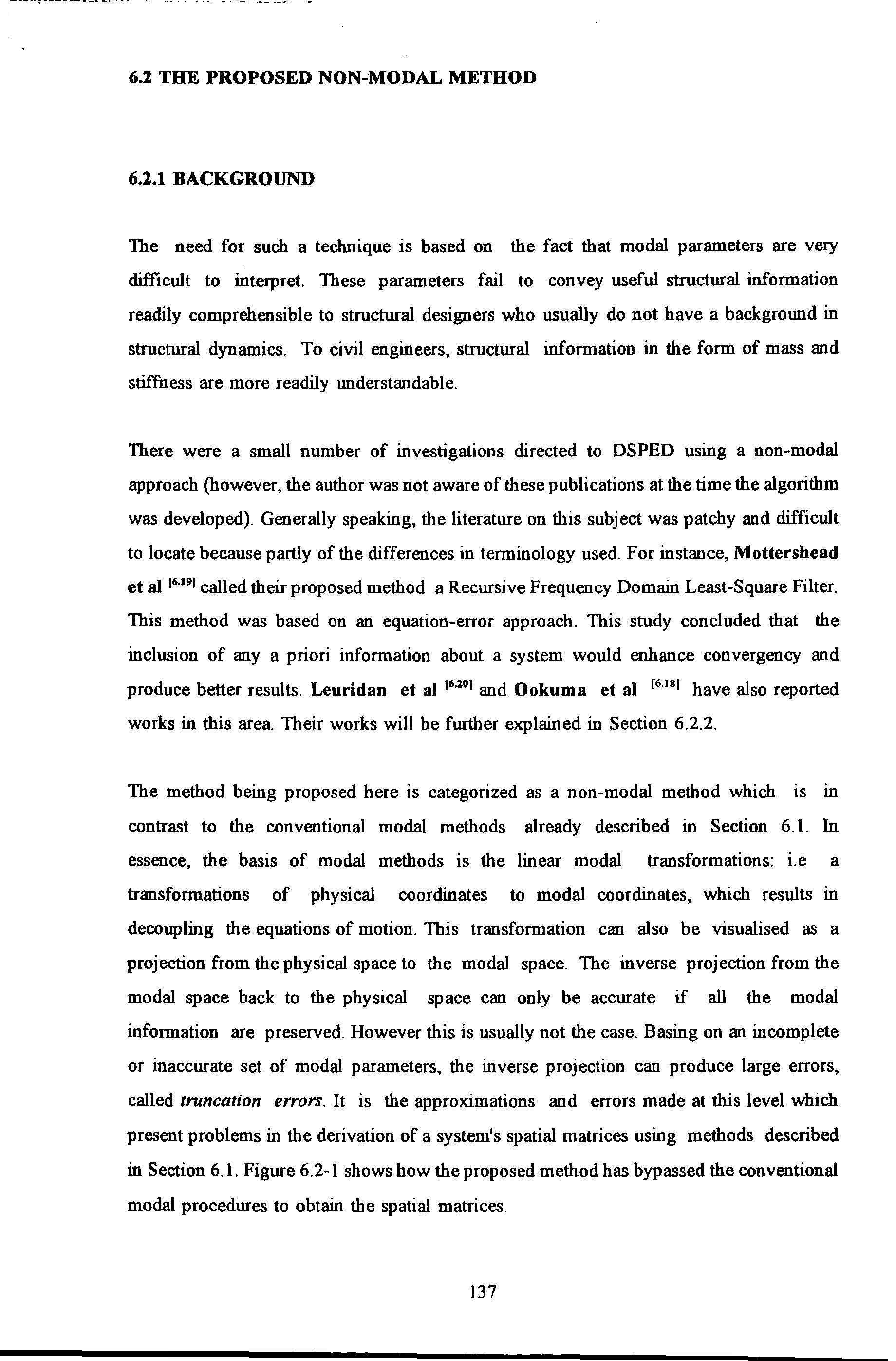
6.2 THE PROPOSED NON-MODAL METHOD
137
FRF (INERTANCE, RECEPTANCE OR STRAIN FRF)
MODAL METHODS TO OBTA1N MODAL AUTIIOR'S PROPOSED

MODELS : SDOF, MDOF, GLOBAL etc. DIRECI' METHOD
SPATIAL MODELS
SYSTEM
IDENTIFICATION
AND
DETERMINATI
MODFll.ING
The inspiration of th is algorithm is accredit ed to N iel se n' s 16 81 work and to the way h e formulated the problem of determining [M] , [C] and [K ] as the solution of simultaneous equations in which the elements of the spatial matrices are extracted to form the unknown vector Hence there is some res emb lance between the two algorithms in these respects
As a s ummary , this algorithm has the following feature s:
l No prior knowledge of the modal parameters is required
2 . No prior knowledge of the mass o f structur e i s requir e d.
3 . No orthogonality i s a ss umed .
4. A 'global' curve fitting t echniqu e is used i .e. in s tead of using only lo cal data, sp atial information from d ata at all oth er m eas urement locations are also used
5 . Consistent modal param eters ar e maintained for each individual
DATA
ACQUISIDON MEASUREMENT
_ _,ll'-
STIFFNESMATRIX s _ _,
Figure 6 2-1 A schematic diagram showing how th e proposed method bypasses the conventional modal procedures to obtain the spati al matrices
138
measurement.
6. The number of measured coordinates does not necessarily have to be equal to the number of measured modes as required in conventional methods.
With this method, less information on individual local test points is required as information can be subordinated by data from measurements at other spatial points of a structure. This spatial reference technique is very useful because more spatial measurements can be carried out at the expense of less detailed local measurements
6.2.2 DEVELOPMENT OF THE ALGORITHM

The general equations of motion of an N degree of freedom system is given below :
where
[M] is then x n system spati al mass matrix
[C] is then X n system spatial viscous damping matrix
[K] is the n X n system spatial stiffness matrix
are then x 1 acce leration, velo city and displacement response vectors respectively
{f(t)} is then x 1 excitation force vector
If the equations are re-written m th e fr eq uency domain by applying Fourier Transformation Y to (6 .2. 2-1), then :
[M] (i(t)} + [C] {.i(t)} + [K] {x(t)} (f{t)} 6.2.2-1
- w2 [M] {X(w)} + j w [C] {X(w)} + [K] {X(w)} {F(w)} 6.2.2-2 139
where {X( ro)} is the vector of .9" of displacement responses in ro

{F(ro)} is the vector of Y of external applied forces m ro
ro is the angular frequency
J is the imaginary unit
Also . the vectors {X(ro)} and {F(ro)} of (6 .2 .2-2) are in general complex quantities :
Using these two equation s and by equating the real and imaginary parts :
If these equations are re-arranged, transposed and separated into the real and imaginary parts as follows :
{X(w)} {XR(w)) + j {X/(w)} 6.2.2-3 {F(w)} {FR(w)) + j {FJ(w)}
{FJ(w)} = ( - w 2 [M] + (K] ) * {X/(w)} + w [C] * { XR(w)} 6.2.2-Sa {FR(w)} = ( - w 2 [M] + [K] ) * {XR(w)} - w [C] * {X/(w)} 6.2.2-Sb
- W {X J(w)}T 140 [M] { XR( w)} T ) ( C] [K] { FR(w) }T (6 .2.2-6a)
Then for a number of frequencies ro 1, ro2 , , ro , Two equations such as Equation (6.2.2-6) can be assembled for each frequency. The completely assembled matrix equations become :
If the number of measured frequency points s satisfy the following criteria : 2 s = 3 n
Then the coefficient matrix denoted by [COEF (ro )] in Equation 6 2 2-7 is square and its proper inverse [COEF (ro)] ·l exists The unknown [M] ,[C] and [K] matrices can be determined by Equation (6 2 2-7) in the normal way However if
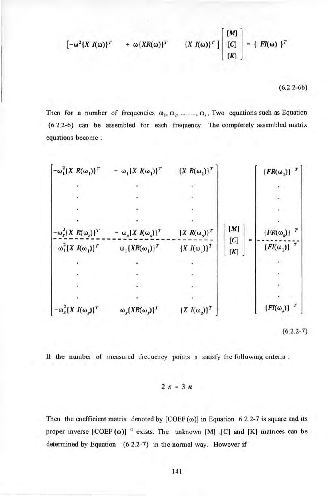
(6 .2.2-6b)
- w;{X R(ws)}T - ws{X l(ws)}T {X R(ws)}T ------------------------------w7tx l(w 1)}r wdXR(w 1)}r {X J(w 1)}r [M] [C] [.K] = {FJ(wl)} T (6 2 2-7)
141
then the coefficient matrix is rectangular and [COEF ( ro)] -t does not exist. In this case a pseudo inverse [COEF (ro )] • is used instead Both Leuridan et al ru•J and Ookuma et al 16 181 have reported using this type of formulation . A different formulation was developed by the author which offers some advantages over the formulation in Equation 6.2.2-7.
Now define the receptance frequency response function ail ro) as
If one excitation force only is app lied at point r such that
then it is convenient to drop the subscript rand redefin e (6 2 2-9) as
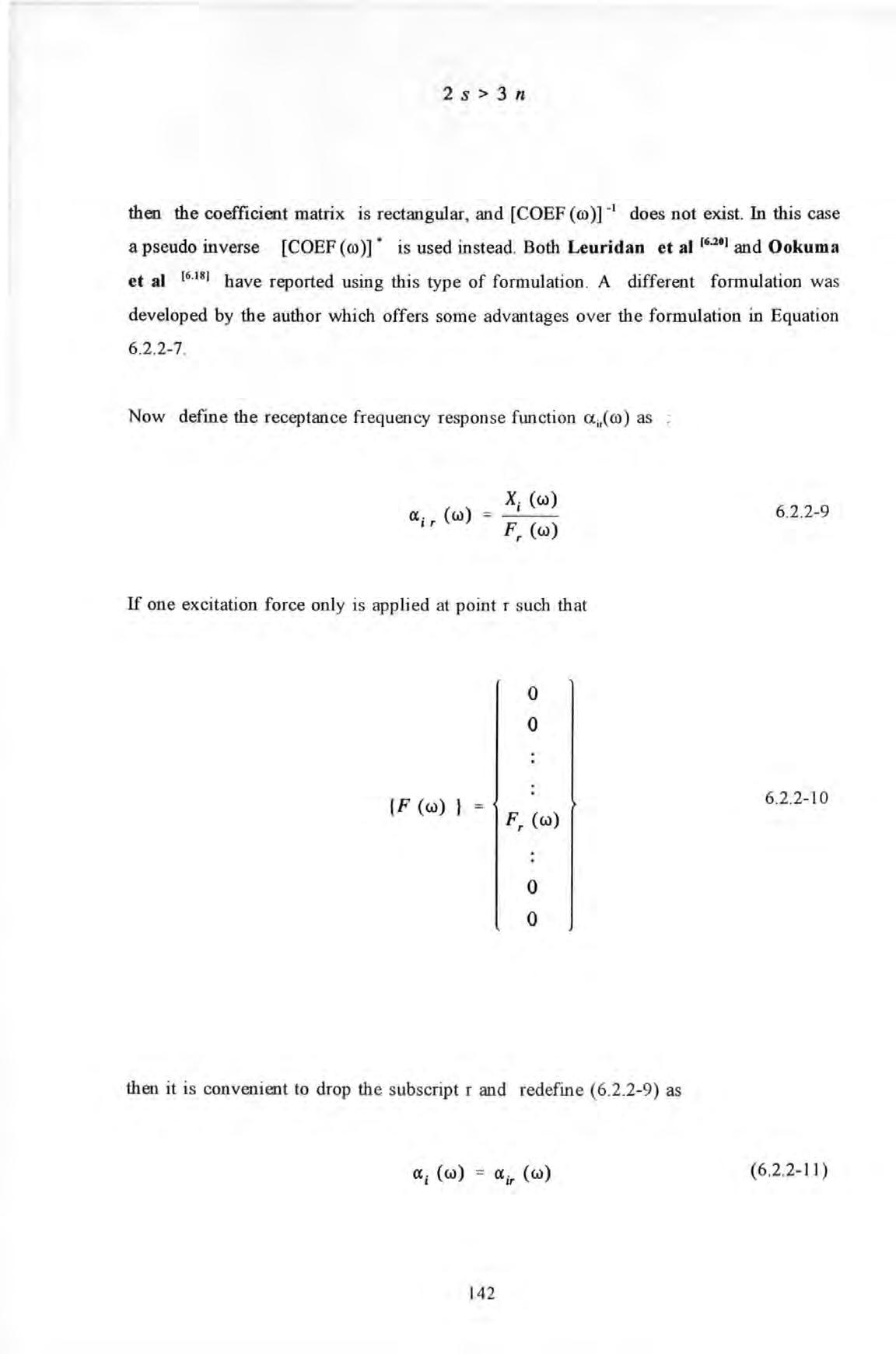
2 s > 3 n
X; (w) F, (w)
{F (w) } 0 0 F, (w) 0 0
142 6.2 .2-9 6 .2 .2-10 (6 2.2-11)
The receptance a;( ro) so defined in ( 6 . 1. 2-1 1) 1s also a complex quantity having real Ra;( ro) and imaginary la;( ro) parts :
Hence by equating the real and imaginary parts of ( 6.2.2-11) :

Using this relationship , Equation (6.2.2-2 ) can be re-written as 0 0 ( -w 2 [M] + jw[C] + [K] ) * a ; (w) = 1 0 0 (6 .2.2-12)
a; (w) = Ra; (w) + j la; (w)
(-w 2 [M] + [K]) * { Ra (w) ) - w [C) * { la (w) ) = 143 0 0 0 1 0 0 6 2.2-13 ( 6.2 .2-14a)
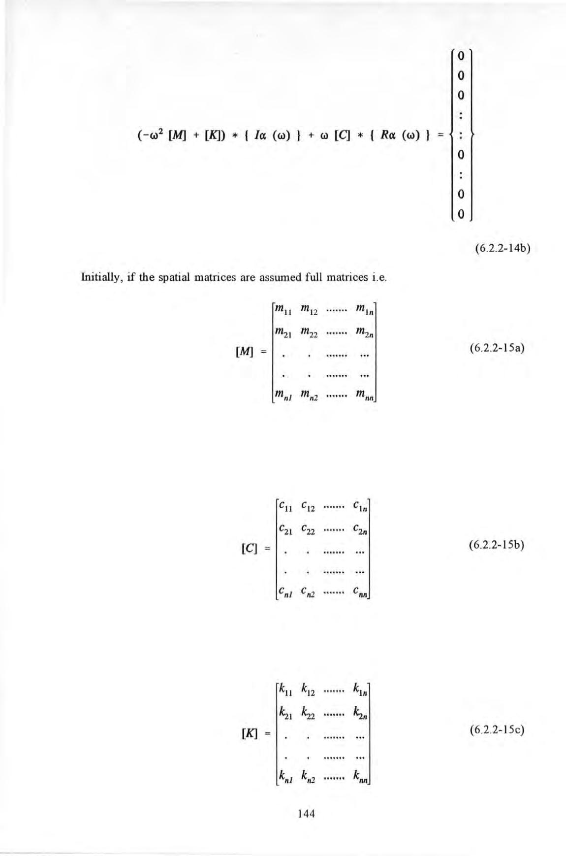
( -C» 2 [M] + [K]) * { la (C») } + C» [CJ * { Ra (C») } Initially , if the spatial matrices are assumed full matrices i.e [M] [CJ = kll kl2 kln 'st 's2 lsn [K] knl kn2 ktlll 144 0 0 0 0 0 0 (6 .2.2-14b) (6.2 2-15a) (6 2 2-15b) (6 2 2-15c)
Then if each element m the matrices is extracted to form an unknown vector (a technique instigated by Nielsen 16 81 in deriving his algorithms as described Section 6.1 .2) :
(Note that Ookuma et al 16 181 have reported using the same approach but the detailed formulation was not presented in their paper) .
Equation (6 2 2-14) now takes the form :

mnn Cu L3 n: X 1)) 6.2.2-16 cnn kll
mu 0 0 mnn 0 Cu [Am) [ Ac] [Ak] 1 6.2 .2- 17 cnn ku 0 0 0 knn 145
where [ Am ] , [ Ac ] and [ Ak ] are of the form
[Am] =
[ - w 2 B ( Ra ( w) ) ]
[ - w 2 B ( la (w) )]
(6 2 .2-19a)
[ -w B (la (w) ) ]
[ w B ( Ra ( w) )]
(6 .2.2-19b)
[ B ( Ra ( w) ) ]
[ B (la (w) )]
(6 .2.2- 19c)
where the matrix functions are defined as follows :
(6 2.2-20a)
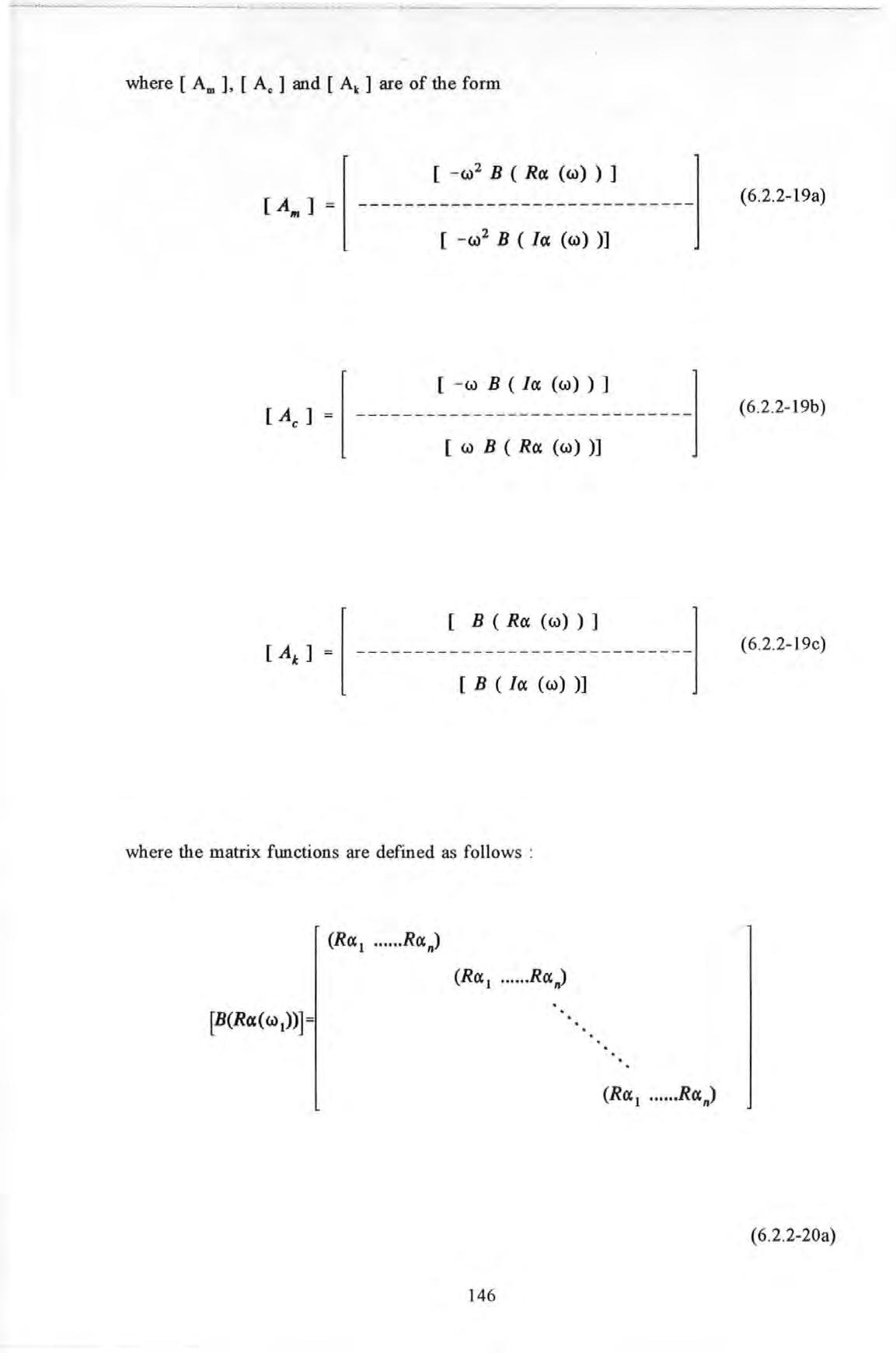
146
It is evident that for each frequency ro, a total of 2n equations such as (6 .2 .2-17) can be formulated. If the frequency response data are available at s different frequencies i e. then the total number of equations available equals 2sn In order to solve the unknowns which now total 3n2 , thence
and
The fully assembl ed matrix equation called system equation is too large to be shown here. The assembling process is similar to that of Equation 6.2 .2-7 . If the number of frequencies available to assemble equation (6 .2.2-17) is more than the statutory minimum i.e 1 5n then the system equations are over-specified and the pseudo-inverse method of solution may be employed In such systems where the spatial matrices may be considered symmetric :

(Ja 1 Jan) (Ja 1 ••••• Jan) (6 .2 .2-20b)
2 s n > 3 n 2
s > 1.5 n
147
Then the number of unknown parameters can be reduced and the upper triangular elements in these matrices only require solution. The number of unknowns in this case is now given by
The use of symmetry has th e advantage of reducing the s1ze of the matrices in the system equation. This in tum simplifies the mathematical operations However, there are situations, such as non-linear systems, in which these matrices may not be symmetrical If the assumption of symmetry is used , the sizes of the unknown vectors {m}, {c} and {k} are each reduced to :
To enforce symmetry and other criteria in the computational process, two method s can be used . The first method is by appending a set of constraint equations to the system equation These constraint equations impo se the following constraints to the system .

0 for all i, j
One such typical constraint equation is given as follows :
(M] = (M]T , (C] = (C]T and (K] (K]T (6.2.2-21a) (6 .2.2-21b) (6.2.2-21c)
n*(n+l) 2
M .. - M
IJ Jl c ij c ji 0 for
i , j K ij K Jl 0 for all i , j
..
all
148
The positions for inserting 1 and -1 are corresponding to the positions of the terms Mu and in the column vector {Y} For those elements which are known to be zero, then constraint equations similar to Eq. 6.2 .2- 23a can be introduced as well. For instance if Mu is zero, then one such typical constraint equation can be written as follows :
However this computational method is quite ineffective A second method was therefore adopted This method requires that all zero valued spatial parameters are eliminated from the {Y} vector and the columns of the coefficient matrix in the system equation corresponding to these terms are deleted This method also has an advantage of reducing the size of the matrices.
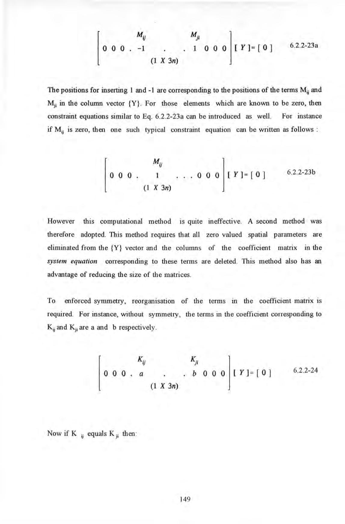
To enforced symmetry, reorganisation of the terms in the coefficient matrix is required. For instance, without symmetry , the terms in the coefficient corresponding to Ku and Kj; are a and b respectively
Now if K u equals K j i then :
Mu 0 0 0 -1 (1 X 3n) Mjl 1 0 0 0 [ y ]= [ 0] 6.2 2-23a
Mu 000 . 1 ... 000 [Y] = (O) 6 2 2-23b (1 X 3n)
Ku 0 0 0 . a
(1 X 3n) 14 9 JS; b 0 0 0 [ y ] = [ 0] 6. 2 2- 24
where {Y} is similar to {Y•} except that the element Kj; has been eliminated and its size decrease by 1. With symmetry, the total number of frequency points required should satisfy the following criteria.
6.2.3 IMPLEMENTATION AND VERIFICATION OF THE ALGORITHM

The algorithm was coded as a computer program in Hewlett P a ckard Basic and verified using a series of computer simulations . The restraints on memory available on the HP 9816 desk-top computer had dictated much of the way the simulations were performed. The computation carried out involves very large matrices and the computer used can only cope with systems of a small number of degrees of freedom.
6.2.3.1 COMPUTER SIMULATIONS
The required FRF data used for the computer simulation were generated from two fictitious vibration systems with known spatial matrices but with no artificially added noise By not introducing noise, error in the results of the computation can be localized to sources such as numerical sensitivity or instability associated which are known to be notorious in most inverse methods ('inverse' method was defined by Bekey 13 91 in Section 3 .3 . 1) .
In order to reduce computational memory requirements, two systems with only a small number of DOF were used.
0 0 0 . 0 0 0 l[y• 1 [ 0 l 6 .2.2-25 1 X (3n-l)
2 s n > 3 n (n + 1) 2
SYSTEM 1 a 3 DOF damped system . 150
The assumed spatial matrices of the two systems are summarized in T ab l es 6.2 .3 .1- 1 to Tab les 6.2 3 1-3 TABLE 6.2.3 . 1-1
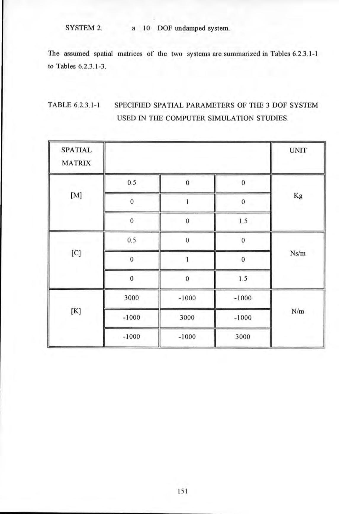
2 a 10 D OF
SYSTEM
undamped system
SPATIAL I MATRIX I [M] I [C] [K ] SPECIFIED
COMPUTER SIMULATI O N STUDIES I UNIT 0.5 I 0 0 0 1 0 Kg 0 0 1. 5 0 .5 0 0 Ns/ m 0 1 0 0 0 1.5 3000 -1000 - 1000 11 N/m - 1000 3000 - 1000 - 1000 11 -1000 3000 151
SPATIAL PARAMETERS OF THE 3 DOF SYSTEM USED IN THE
TABLE 6.2.3 . 1-2
THE SPECIFIED MASS MATRIX OF THE 10 DOF SYSTEM USED IN THE COMPUTER SIMULATION
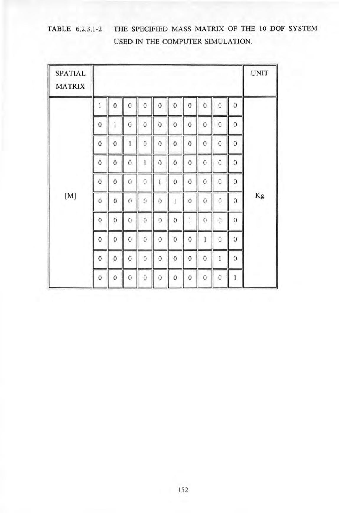
IU 152
TABLE 6 2 3 1-3
SPATIAL
MATRIX
A FRF data set was synthesi z ed for each degree of freedom (or each spatial point) These data were effectively a set of receptance spectra which would have been obtained from experiment rather than synthesized in this way For both SYSTEM 1 and 2 , the receptance spectra were synthesized by assuming the single force input was applied at the spatial point No 1
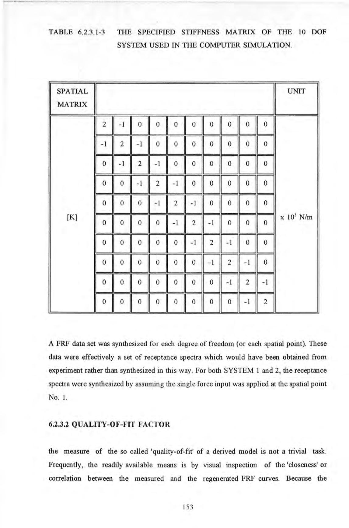
6.2.3.2 QUALITY-OF-FIT FACTOR
the measure of the so called 'quality-of-fit' of a derived model is not a trivial task. Frequently , the readily available means is by visual inspection of the 'closeness' or correlation between the measured and the regenerated FRF curves. Because the
THE SPECIFIED STIFFNESS MATRIX OF THE 10 DOF SYSTEM USED IN THE COMPUTER SIMULATION.
LJ
GGGGGGGGG 2
[K] x 103 N /m
153
assumed spatial matrices used m the computer simulation are known then a direct comparison between the derived and the assumed matrices can be used to indicate how good or bad a model is A quantifier or indicator QF 1 can be used and has been defined as follows:
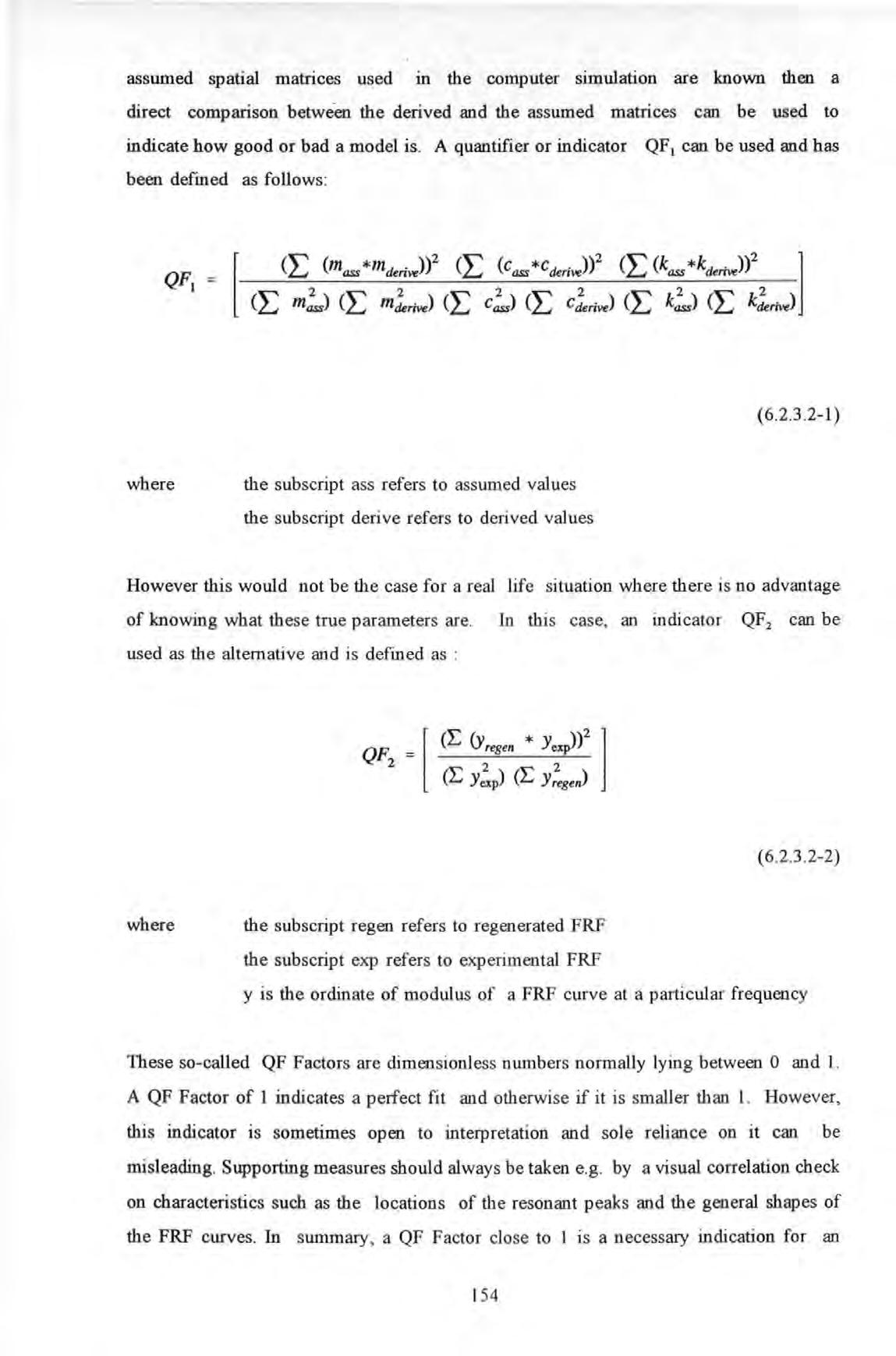
the s ub scri pt ass refers to ass umed values
the s ub scri pt derive refers to derived values
However this would not be the case for a real life si tuation where there is no advantage of knowing what these true parameters are. In this case, an indicator QF2 can be used as the alternative and is defined as :
the subscript regen refers to regenerated FRF
the subscript exp refers to experimental FRF
y is the ordinate of modulus of a FRF curve at a particular frequency
These so-called QF Factors are dimensionless numbers normally lyin g between 0 and 1. A QF Factor of 1 indicates a perfect fit and otherwise if it is smaller than 1. However, this indicator is sometimes open to interpretation and sole reliance on it can be misleading Supporting measures should always be taken e g by a visual correlation check on characteristics such as the locations of the resonant peak s and the general shapes of the FRF curves In summary , a QF Factor close to 1 is a necessary indication for an
where [ (L (mass *mtkrive)f (L (Cass*Ctkrive)? (L (kass*ktkrive)? ] (L m!,J (L m!rive) (L c!s) (L c!rive) (L k!s) (L k!nve)
( 6.2 .3 .2-1)
QF,
(L (yrege n * (L Y (L Y! 8 e,J
where
[
(6.2 .3 .2-2)
154
6.2.3.3 RESULTS
The simulation was performed to investigate the validity of the algorithm under a mixed combinations of the following different scenarios :
SCENARIO 1
The selected data points were well distributed over the range of frequencies covering all the modes.
SCENARIO 2
The selected data points were concentrated at a narrow range of frequencies covering fewer modes
SCENARIO 3

The full data set for al l the spatial points was used
SCENARIO 4
A smaller data set chosen from some of the spatial points was used
In general, the accuracy of the derived spatial matrices was found to be affected in various ways by all four scenarios. Especially in SCENARIOS 1 and 3, exact spatial matrices (both the forms and values of the matrices) and QF Factors of l for both SYSTEM 1 and 2 were obtained if the following rules were followed :
a at least 2 data points on either side of each resonant peak were chosen
b the data points chosen did not cover more modes than the order of matrices to be derived
The results for SYSTEM I are given in Figures 6 2 3 3-1 to 6.2.3 3-3 Good results are indicated by total eclipse of the original curves (plotted with solid dots) by the regenerated curves (plotted with asterisks).
accurate
but
model
not sufficient.
155
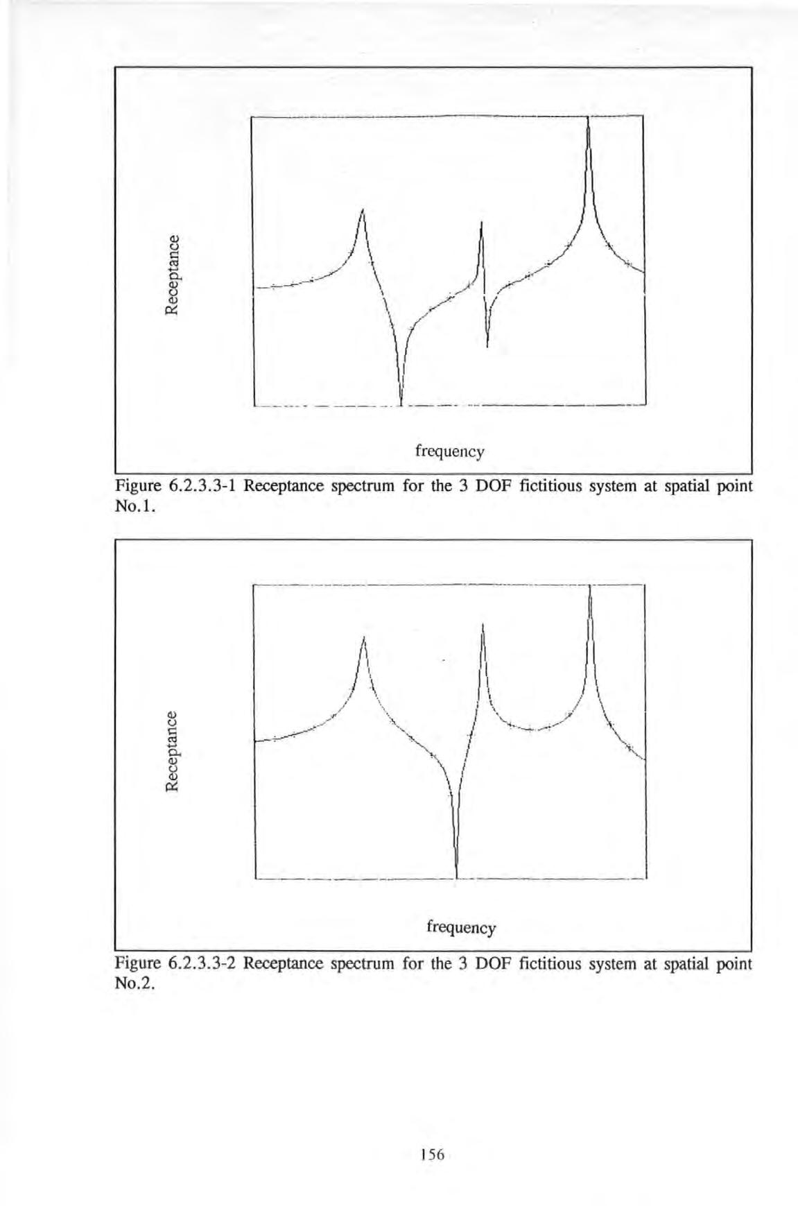
I\J \ __../ \ .t ' \(/ r -__ _j' __ -frequency
r---· - ------- ---------1 )\, . )\ I / \, / ' , / \ / "'\ I \ '--------frequency
Figure 6.2.3.3- 1 Receptance spectrum for the 3 DOF fictitious system at spatial point No.l.
15 6
Figure 6.2.3.3- 2 Receptance spectrum for the 3 DOF fictitious system at spatial point No.2.
frequency
However, more acute reduction in accuracy was found to occur in SCENARIOS 2 and 4 This is illustrated by the results obtained from SYSTEM 2 and given in Tables 6 2 3 3-1 and 6 2 3 3-2 In thi s simulation run , a reduced mod el of order 6 was derived using 6 out of the 10 FRF data set. The 6 frequency points chosen cover 3 out of the 10 modes presented

Q) (J c: Ct1 ..... 0.. Q) (J Q) A:: J / / / I \ \ / 1 '------ -------J-.----.JI
Figure 6.2.3.3-3 Receptance spectrum for the 3 DOF fictitious system at spatial point No.3 .
6EJEJI-297.331EJB [M] EJEII-574.221EJEJ 18 38 6EJEJEJ6 11.42 157
TABLE 6 .2 .3 .3-1 THE REDUCED ORDER 6X6 MASS MATRIX OF THE 10 DOF FICTITIOUS SYSTEM DETERMINED BY THE ALGORITHM.
TABLE 6.2 .3 .3-2
THE REDUCED ORDER 6X6 STIFFNESS MATRIX OF THE 10
DOF FICTITIOUS SYSTEM DETERMINED BY THE ALGORITHM
The original and the regenerated curv es are plotted in Figures 6 .2 .3 .3-4 to 6.2.3.3-7 for 4 out of the 6 spatial points used .
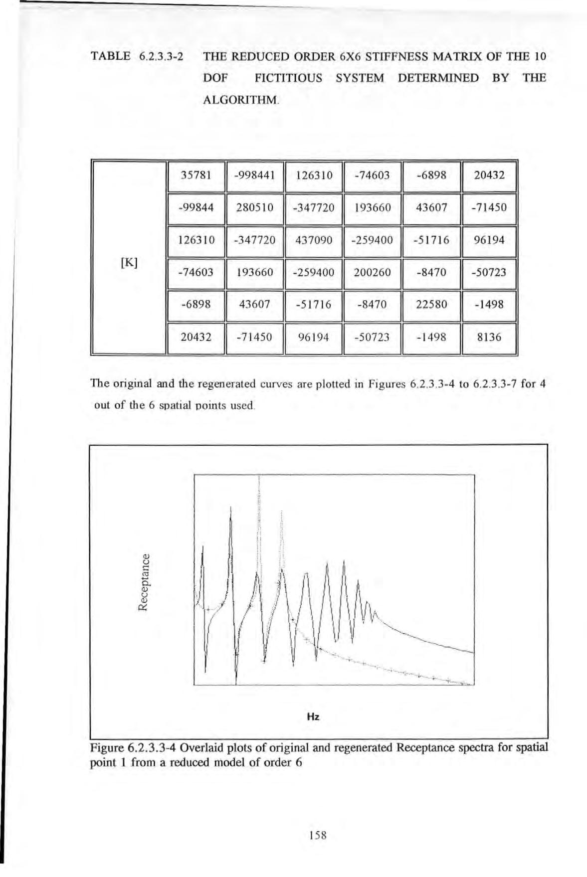
[K]
I:I l J. ·; ·· ' a .•• I t I 'd "+ \f. "-·---.._ I >· ... . · I , ,. t• •• •:-. • i·· _ Hz
158
Figure 6 . 2 .3 .3 -4 Overlaid plots of original and regenerated Receptance spectra for spatial point 1 from a reduced model of order 6
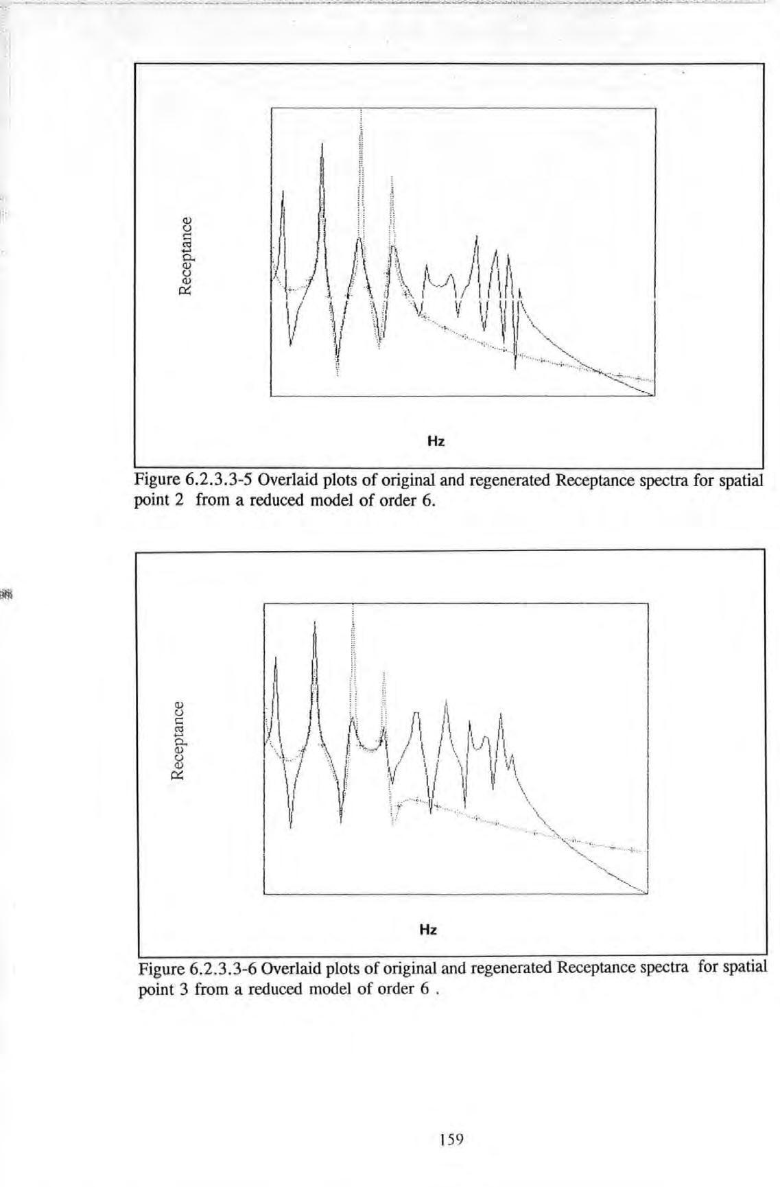
Hz
Figure 6.2.3.3-5 Overlaid plots of original and regenerated Receptance spectra for spatial point 2 from a reduced model of order 6. Hz
159
Figure 6.2 .3.3-6 Overlaid plots of original and regenerated Receptance spectra for spatial point 3 from a reduced model of order 6 .
Although the original spatial matrices are known to be tri-diagonal , full matrices are used to account for the reduction of the order of the model from I 0 to 6 The figures show that the regenerated curves only match the original curve in the narrow range covered by the 6 chosen data points.
6.2.4 PRACTICAL APPLICATIONS
Apart from fictitious systems, the algorithm was also applied to a variety of real systems using experimental data obtained mainly from laboratory tests Two real systems : a 4-mass torsional system (discrete) and a cantilever beam (continuous) were used.
The tests were carried out at the Structural Dynamic Laboratory of the Royal Naval Engineering College Plymouth . The instrumentation used in these l aboratory tests was quite separated from those used for full scale tests. As the data were of interest here, specific details on this experimentation are not to be di scussed any further. Only a schematic diagram showing the test set- up and the list of equipment used are given in Figure 6.2.4-1.

- --· Hz
Figure 6.2.3.3-7 Overlaid plots of original and regenerated Receptance spectra for spatial point 4 from a reduced model of order 6 .
160
The torsional system was constructed by attaching fou r lumped masses along the length of a steel rod which was clamped rigidly at both ends as shown schematically in Figure 6.2.4-2. A series of roller bearings were spaced along the length of the rod These bearings restrain lateral movement and allow only rotational (twisting) freedom . So the total number of vibrational modes was effectively confined to only 4 The system was excited by a miniature electromagnetic shaker through an attachment to the mass m 1 All the modes of vibration involved were covered in the measurement. The spatial matrices obtained for this system are given in Table 6.2 .4- 1 for the undamped case and in Table 6.2.4-2 for the damped case These matrices form a complete model Correlation (for the undamped case) between the measured and the regenerated FRF curves for 2 of the masses measured are given in Figures 6 .2.4-3 to 6.2.4-4 .
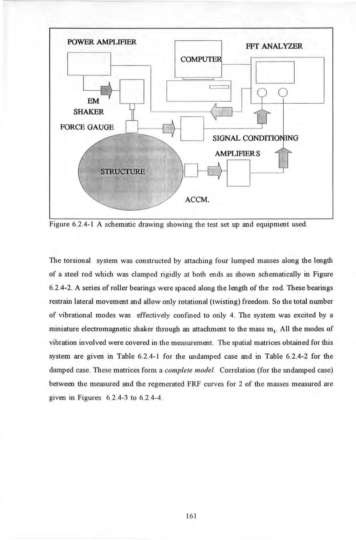
SHAKER FORCE
S'IRUCfURE FFf ANAL"YZER COMPUTE D ACCM. 0
AMPLIFIERS
POWER AMPLIFIER
GAUGE
SIGNAL CONDmO
G
Figure 6 2.4-1 A schematic drawing showing the test set up and equipment used
161
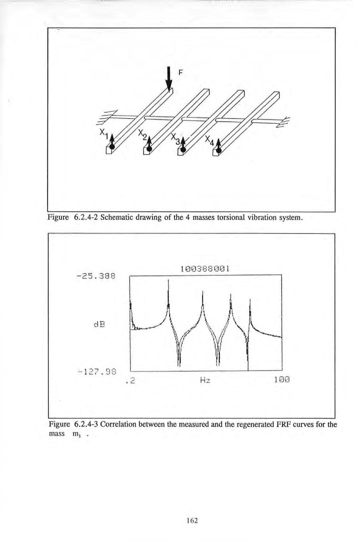
F
dB 1 .-, -, ra -, - l,::. / • .::::; :::a
Figure 6.2.4-2 Schematic drawing of the 4 masses torsional vibration system. 1 00 38:3001 -25.388
1 • 162
Figure 6 .2. 4-3 Correlation between the measured and the regenerated FRF curves for the mass m
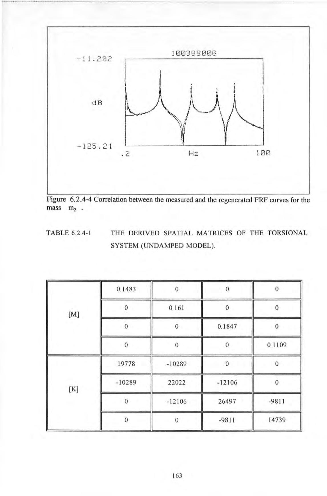
1 003 8 8 0\?:16 -11.282 I I l J I I \ 1 I 1 l I L-A "'\ .. \ '-\Ill \ "-._ ' I I I dB -125.21 I .2 Hz
Figure 6.2.4-4 Correlation between the measured and the regenerated FRF curves for the mass m2 •
I [M] I I I [K]
TABLE 6.2.4-1
(UNDAMPED MODEL) 0 1483 0 0 11 0 0 0 161 0 0 0 0 0.1847 0 0 0 0 0 1109 19778 -10289 0 0 -10289 22022 -12106 0 0 -12106 I 26497 -9811 0 0 11 -9811 14739 163
THE DERIVED SPATIAL MATRICES OF THE TORSIONAL SYSTEM
THE DERIVED SPATIAL MATRICES OF THE TORSIONAL SYSTEM
Because the system is a torsional one, the corresponding equation of motion should all be in terms of moment of inertia instead of mass and similarly for the other quantities. The [M] , [C) , [K] are used here to denote inertia , damping and stiffness in the most general sense.
The second system tested was a beam (a contin uou s sys tem) which possesses an infinite number of vibration modes Any approximation based on a low-order, discretized and small DOF model are as usual subjected to truncation errors. These tests were intended to study precisel y the severity of these e rrors caused by discretization and truncation of a real system .
Data were obtained from a steel beam with the following dimen si ons : 4 .88 mm x 24.85 mm in cross section and 696 mm in length The beam was clamped at one end and
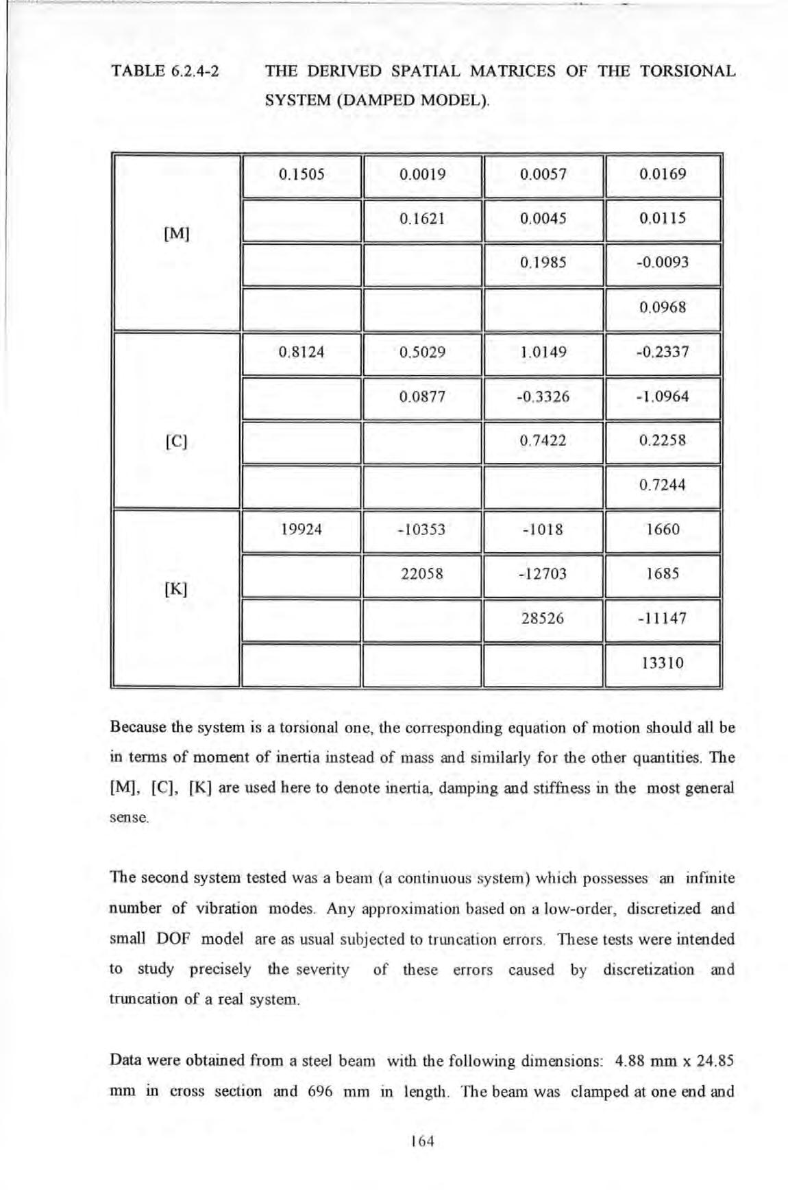
TABLE 6 .2 .4-2 [M] [C) [K]
(DAMPED MODEL) 0.1505 11 0 0019 11 0 0057 0 .0169 I 0 1621 11 0 0045 0 .0115 11 0. 1985 -0 0093 0 0968 0 .8124 0.5029 1.0149 -0.2337 0 0877 -0 3326 I -1 0964 0.7422 0 2258 0 7244 19924 - 10353 - 1018 1660 l 22058 -12703 1685 28526 -11147 13310
164
lateral responses at six designated locations covering the length of the beam were measured usmg Bruel & Kjaer piezoelectric accelerometers and signal conditioning hardware. A single excitation force was applied at the spatial point No . I near the support end using an electromagnetic shaker. Figure 6 .2.4-5 show a schematic drawing of the beam test arrangement. FRF data covering a frequency band of 4 to 1200 Hz and 6 modes were obtained for analysis Because these tests were carried out in a well controlled laboratory environment, very high quality data was able to be obtained
Since the beam was very lightly-damped, the assumption of zero damping was thought to be justifiable. This assumption was also necessary, beca use the resulting computational problem would exceed computer memory limi t if otherwise. Four models were obtained from the four conditions listed in Table 6 2.4-3
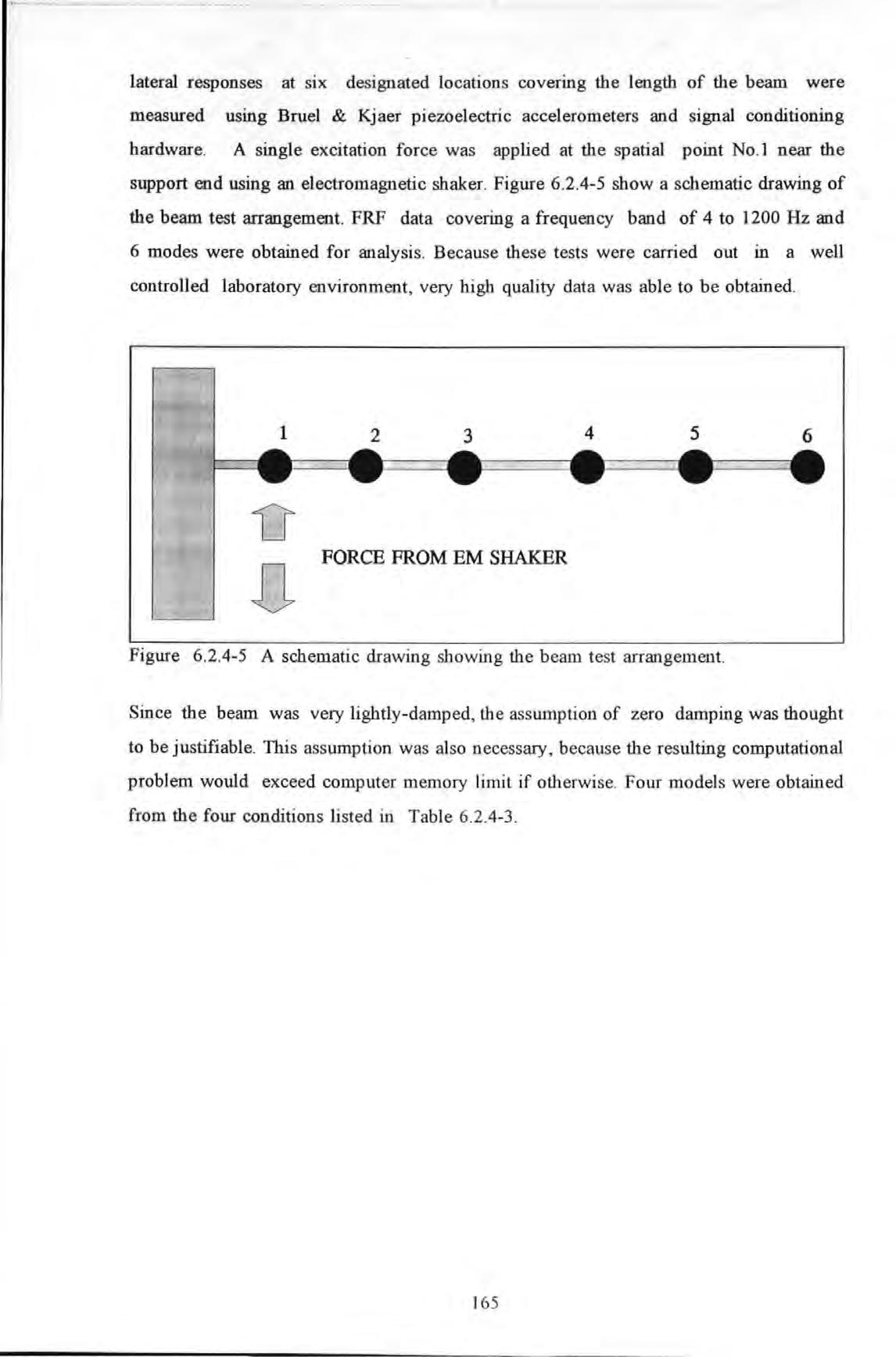 D DFORCE FROM EM SHAKER
4 5
D DFORCE FROM EM SHAKER
4 5
6
Figure 6.2 4-5 A schematic drawing showing the beam test arrangement.
165
TABLE 6.2.4-3 . DETAILS OF THE ANALYSIS CONDITIONS TO DERIVE THE SPATIAL MODEL OF THE BEAM.
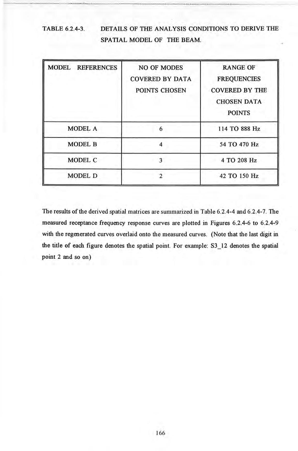
MODEL REFERENCES NO OF MODES RANGE OF COVERED BY DATA FREQUENCIES POINTS CHOSEN COVERED BY THE CHOSEN DATA POINTS
The results of the derived spatial matrices are summarized in Table 6 2.4-4 and 6.2.4-7 The measured receptance frequency response curves are plotted in Figures 6.2.4-6 to 6.2.4-9 with the regenerated curves overlaid onto the measured curves. (Note that the last digit in the title of each figure denotes the spatial point. For example : S3 12 denotes the spatial point 2 and so on)
MODEL A 6 114 TO 888Hz MODEL B 4 54 TO 470Hz MODEL C 3 4 TO 208Hz MODEL D 2 42 TO 150Hz
166
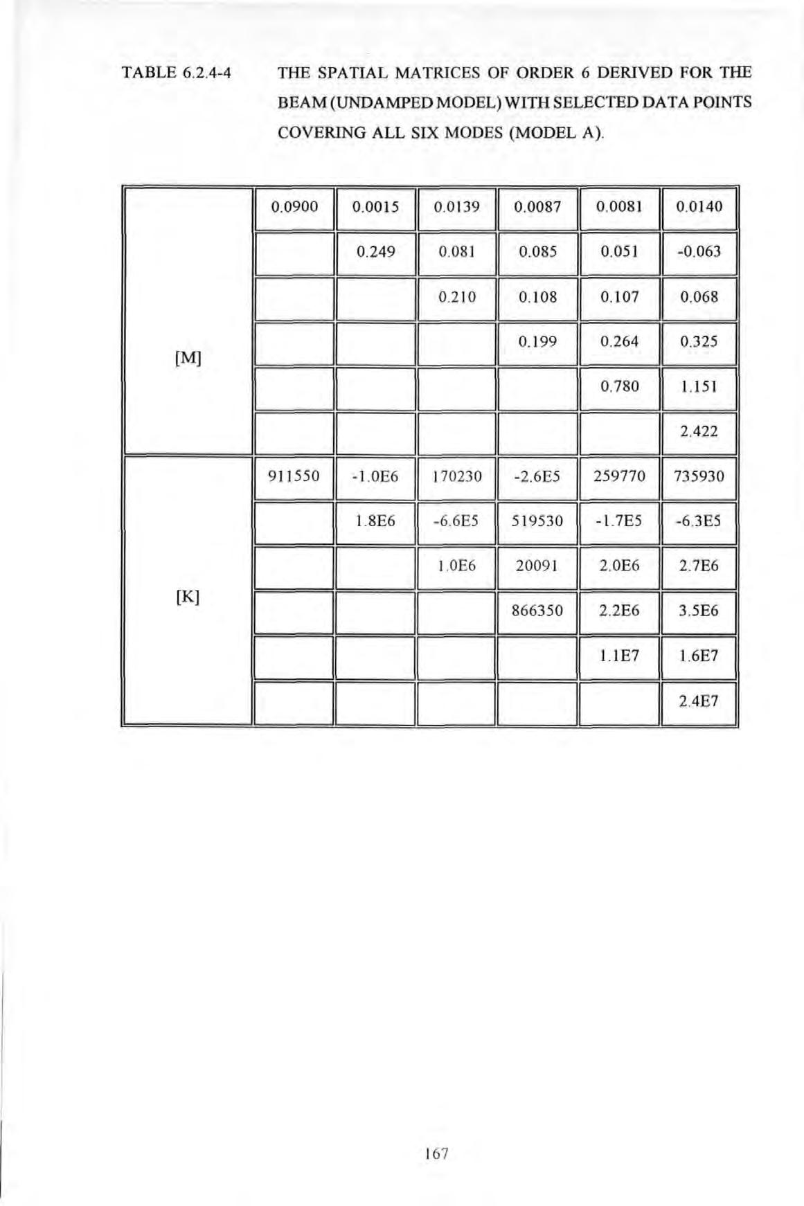
TABLE 6 .2.4-4 [M] [K] THE SPATIAL MATRICES OF ORDER 6 DERIVED FOR THE BEAM (UNDAMPED MODEL) WITH SELECTED DATA POINTS COVERING ALL SIX MODES (MODEL A) . 006666 000666 000066 000006 259770 11 735930 1 OOEJEJEJ6 0001866 350 166 000066 OOOOOEJ 167
TABLE 6 .2.4-5
THE SPATIAL MA TRJCES OF ORDER 6 D ERIVED FOR THE BEAM (UNDAMPED MODEL) WITH SELECTED DATA POINTS COVERING ONLY FOUR MODES (M ODEL B) .
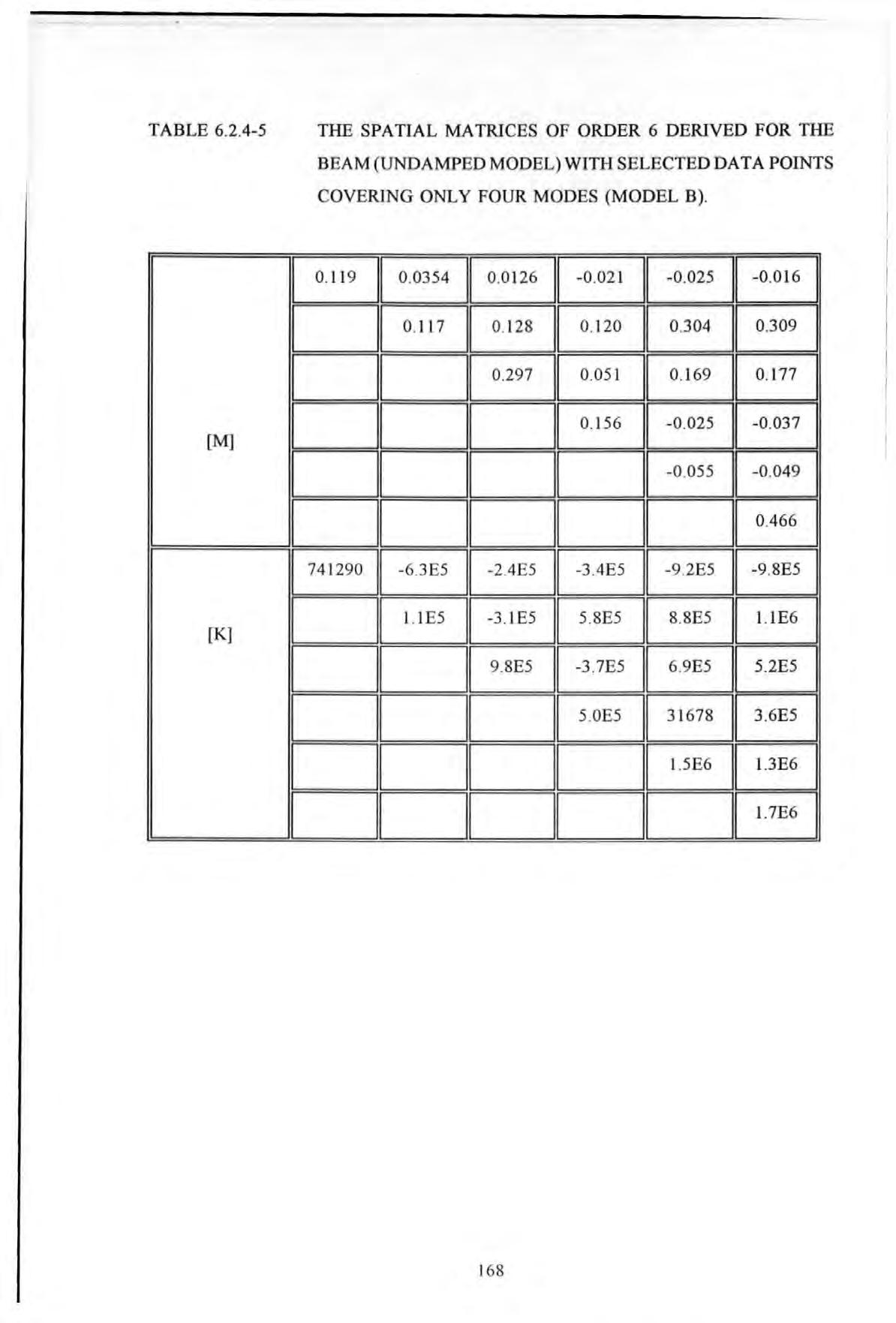
[M] [K]
6666EJ6 066666 DDEJEJ66 DDD6EJ6 DDDDEJ6 DDDDD6 DEJEJEJEJ6 DDEJEJEJ6 DDDEJEJ6 DDDDEJ6 DDDDD6 168
TABLE 6 .2.4-6
THE SPATIAL MATRICES OF ORDER 6 DERIVED FOR THE BEAM (UNDAMPED MODEL) WITH SELECTED DATA POINTS COVERING ONLY THREE MODES (MODEL C) .
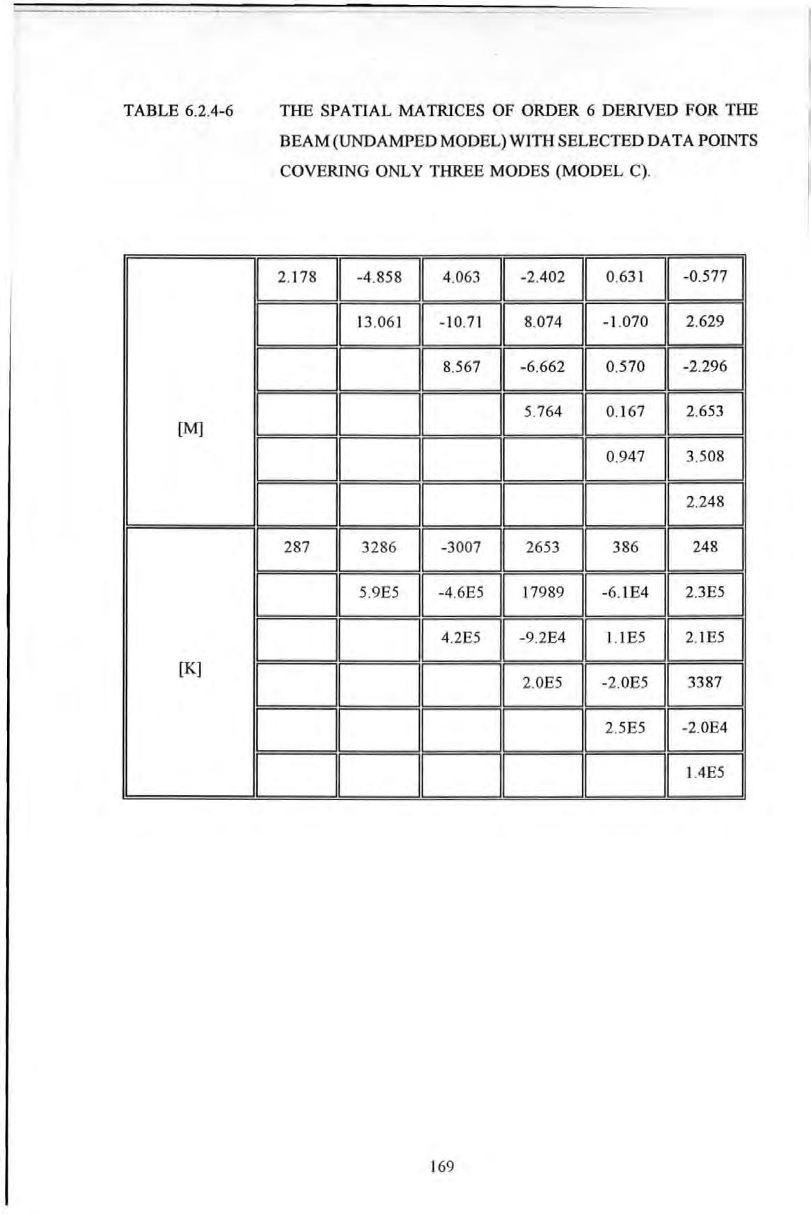
[M] [K)
666666 OEJ666EJ 000666 000066 000006 006EJ66 00006EJ 000006 169
TABLE 6.2 .4-7
THE SPATIAL MATRICES OF ORDER 6 DERIVED FOR THE BEAM (UNDAMPED MODEL) WITH SELECTED DATA POINTS COVERING ONLY TWO MODES (MODEL D) .
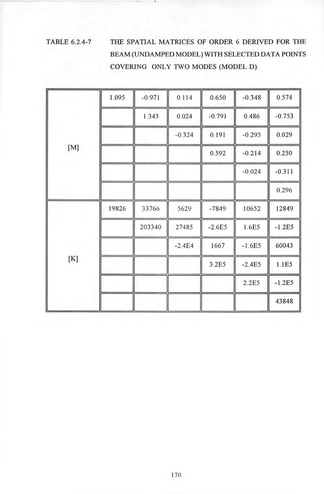
[M] [K]
EJEJ6EJEJ6 D6EJEJEJ6 DDEJ6EJ6 DDDEJEJ6 D DDDEJ6 DDDDD6 01203340 DDEJ6EJ6 170
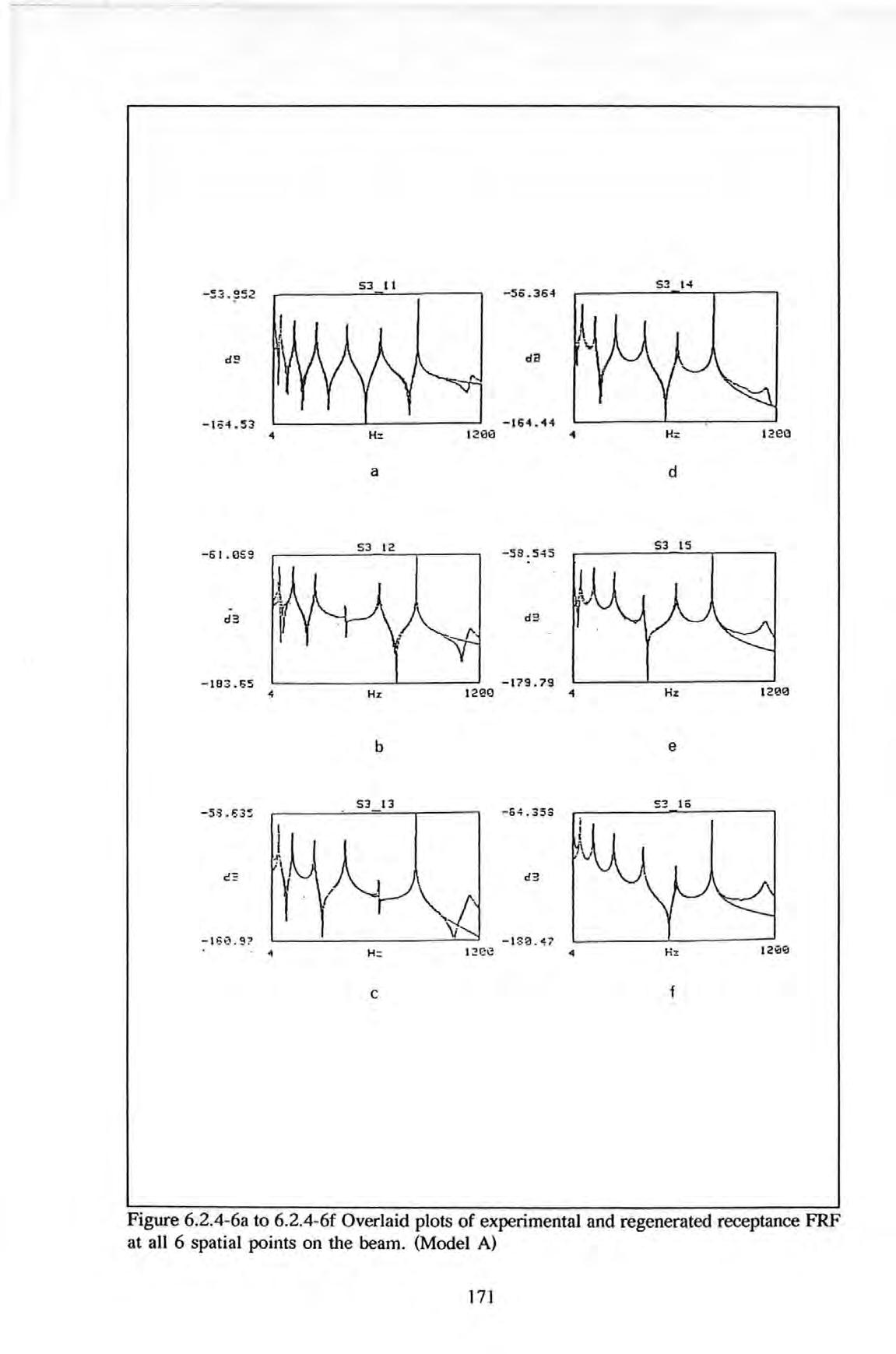
53 11 H:: a d -61.CS9 53 12 -58.545 d3 dE -183.65 -179.79 .; Hz 12!!!t.l Hz 12!!!0 b e 53 13 53 16 - -64 35S c!? d3 c f
171
Figure 6 2.4- 6a to 6 2.4-6f Overlaid plots of experimental and regenerated receptance FRF at all 6 spatial points on the beam. (Model A)
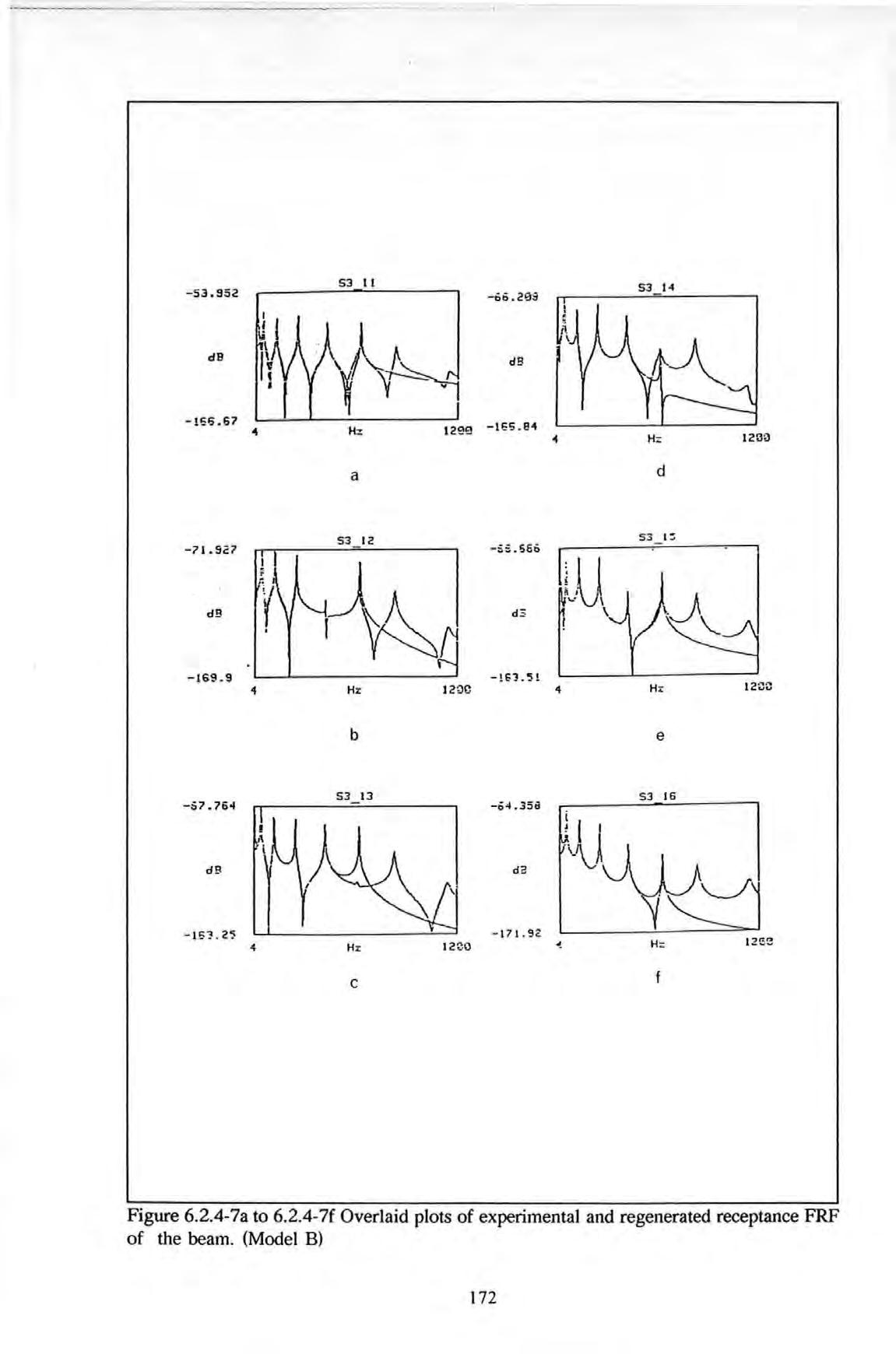
53 ll -53.952 dB H: t20il -166.67 12ee -tes . e1 1 a d 53 12 53 1::: - 71.527ilU ..... \ dB d5 \ r l'l ! -169.9 -!!;1.'5! 1 H:r 12l)C 1 H:r b e 53 13 53 16 -57.76o! - -1)4.3513 j t dll dil . "-----./' -171 92 -----= -IS1 25 t2Ge 4 Hz 12CO H: c
172
Figure 6.2.4-7a to 6.2.4-7f Overlaid plots of experimental and regenerated receptance FRF of the beam. (Mode l B)
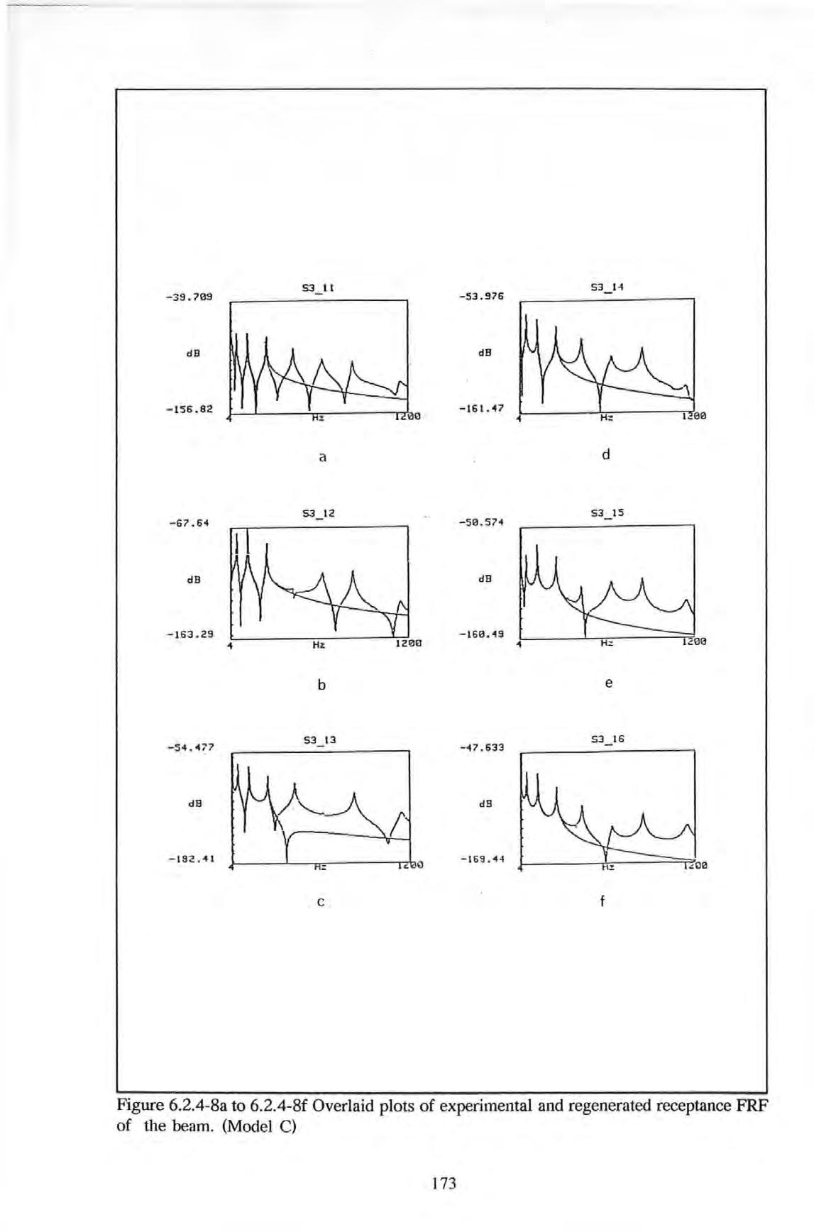
-39 709 53_11 -53.976 53_14 dB dB -156.82 -161.47 a d -67.64 53_12 -5 0.574 53_15 dB dB - 163.29 -160.49 4 b e 53 13 5316 -5-4.4;'7 - -47.633 dB d9 I - 192 41 -169.4-4 = c. c f
17 3
Figure 6.2.4-Sa to 6.2.4-Sf Overlaid plots of experimental and regenerated receptance FRF of the beam. (Model C)
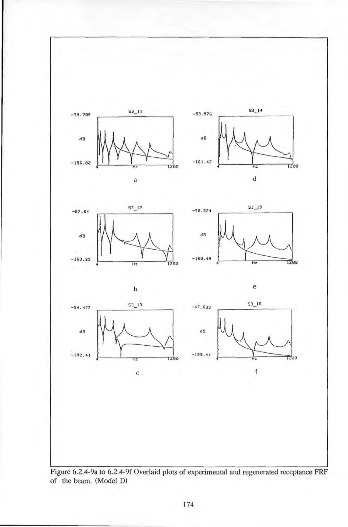
-39 709 53 11 -5 3.976 dB dB -156.82 -161.47 a d 53 I S 53 12 -50.574 -67 .64 dB dB -163.29 -160.'49 4 b e 53 13 5316 -54.477 - -'17.633 dB d9 -169 4-1 c
174
Figure 6.2.4-9a to 6.2 .4 -9f Overlaid plots of experimental and regenerated receptance FRF of the beam (Model D)
From the simulation, the results show that the exact spatial matrices (in terms of their values as well as the form of these matrices) can be obtained providing that the order of the matrices are chosen exactly and the frequency points are chosen appropriately However with some bad choices, incorrect results are obtained In general, the accuracy of the proposed method is found to be very sensitive to those factors covered by the scenarios studied. No hard-and-fast rule is available which can guarantee good results . The errors are due to modelling error and a computational problem called ill-conditioning. The latter is due to the way the equations is posed and is known to be associated with most inverse methods .
From the practical experiments conducted on the 4-mass discrete system and the beam, using both SS (Stepped-Sine) and PRBS (Pseudo-Random -Binary-S equence) excitation methods, good results were also obtained. The stiffness and particularly the mass matrices obtained agree favourably to those estimated by other means For instance, the spatial matrices obtained by Hallett 1' .2 11 , who conducted an independent experiment on the same 4-mass torsional system using conventional modal approach, are given in Table 6 .3-1
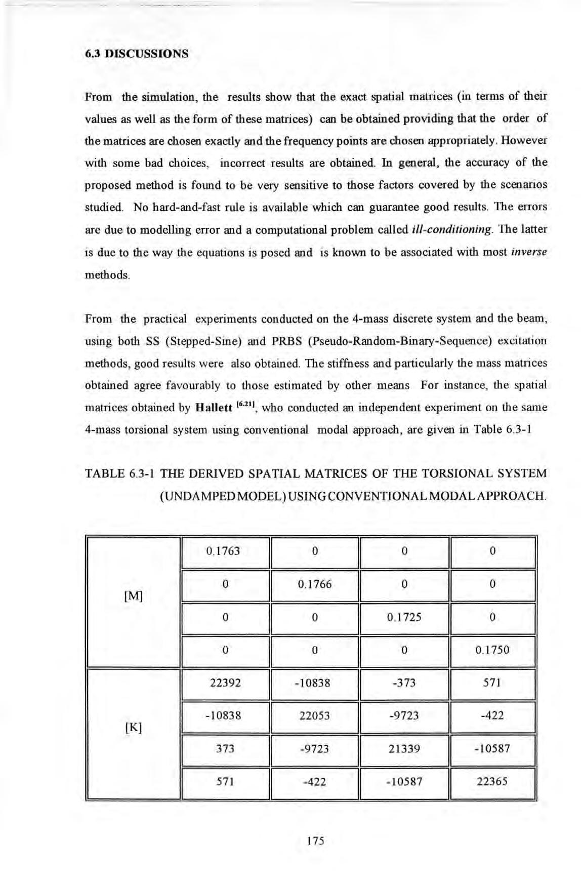
6.3
DISCUSSIONS
(UNDAMPED MODEL) USING CONVENTIONAL MODAL APPROACH. 0 1763 0 0 0 0 0. 1766 0 0 [M] 0 0 0 . 1725 0 0 0 0 0.1750 22392 -10838 -373 571 -1083 8 22053 -9723 -4 22 [K] 373 -9723 21339 - 10587 I 571 -422 -10587 22365 175
TABLE 6 3-1 THE DERIVED SPATIAL MATRICES OF THE TORSIONAL SYSTEM
The values in these matrices compare well with those in Tables 6.2.4-1 and 6.2.4-2. In the case of the beam, the sum of the diagonal terms in the mass matrices in the various models derived are in the same order of the actual physical mass of the beam. So these results confirm that the proposed method is practical for these applications.
The proposed method has a number of features which are considered to be advantageous. First of all, the method requires only a very small number of frequency data points to work. These points can be far apart from each other along the frequency axis. Therefore the method is not suffering from the problem of lack of frequency resolution as the modal methods are. Secondly, the frequency data points required do not need to be very close to those at resonance, so the usual problem of inaccurate measurements around resonance is alleviated. Thirdly, the process of curve-fitting is performed globally utilizing data available from all the spatial points in one operation. This utilization of spatial infonnation is very different from other curve-fitting techniques which use only local infonnation.
It is apparent that the concept of mode of vibration is discarded all together in the implementation of this technique. Unlike modal methods wherein the form of damping is critical in deciding the ease of subsequent analysis (i.e. whether to pursue a real or complex mode analysis), there is no extra difficulty involved in dealing with viscous damping when using the proposed method.
This spatial approach was first published in the Proceedings of the 71h International Analysis Conference (see Tsang and Rider 1 6 14 1 ). Later, Lee IUS! , Lee and Dobson '6"161 extended this method by considering higher order terms and introducing an alternative set of spatial matrices known as [P], [Q], [R], [S] which are similar to the [M], [C], [K] matrices used here. Their method was also based on the direct least square formulation proposed here.

176
The proposed algorithm possesses a number of desirable characteristics as discussed. Above all, it enables the derivation of the spatial matrices directly without using the conventional modal procedures. For simple structures, the algorithm has been proven valid and successful. Mass, stiffness and damping matrices of these structures are much easier to interpret than modal parameters because of the apparent physical meanings they attach. However for complex structures, more research is still required for such applications. This work has shown that spatial matrices determination can be regarded as a main-stream approach rather than a derivative of the modal approach.

6.4 CONCLUSIONS
177
CHAPTER 7
FULL SCALE FORCED VffiRA TION TESTS ON THE BRITISH RAIL BUILDING
7.0 INTRODUCTION
This chapter reports the results and fmdings of the full scale forced vibration tests performed on the British Rail Inter-city House, Plymouth (designated as BR Building). These tests were carried out mainly for the purpose of trying out the new exciter and other equipment described in Chapter 4. Because this building had previously been tested by other investigators, results from the new tests can be used to compare with those from the previous tests.

Many of the experimental techniques and procedures used in the new tests followed closely those used and reported in other investigations (such as those undertaken by BRE as described in Chapter 2). Many operations such as setting-up, controlling and taking readings of instruments were still being carried out manually because a computer-aidedtesting facility had not been incorporated into the instrumentation system. The experience had subsequently inspired several developments and improvements in the instrumentation and the testing technique for future tests.
Analytical modelling of the structure using the finite element method was also carried out to assess the strength and weakness of this method. The model was prepared and analyzed to determine its theoretical vibration characteristics. Using only simple beam elements and exercising appropriate approximations, the theoretical results were found to reconcile with those from real measurement at large. However disagreements, as always, still exist.
178
7.1 DESCRIPTION OF THE STRUCTURE
This building is situated in the city of Plymouth. It is eleven storeys high and used as office accommodation (the tenth floor housed the plant rooms only and was not accessible for measurement) . It was constructed some 30 years ago and was a subject of forced vibration research on a number of occasions during the 1970•s Details of these tests were reported by Williams 11 • 11 , Jeary and Sparks 12 1 • 2 .3 9 1·
The structure is rectangular 45 m x 13 m in plan and 47 m high. It was constructed with reinforced concrete on a large raft type of foundation . Figure 7. 1-1 gives a photographic view of the structure
Th e architectural floor plan is rep etitive f r om the f i rst to the ninth floor as shown in Figure 7. 1-2 .
 FIGURE 7 1-1 A photographi c view of the BR building
179
The building is symmetrical about the NS principal axis and has four reinforced concrete shear cores : among which one is located near the northern end and the other three near the southern end of the building. Three shear cores form the three lift shafts and the other one as a closed box section for utilities to run through. These structural elements stretch along the full height of the building. A pair of external planar shear walls are situated at each of the northern and southern ends. These walls run parallel to the short (EW) direction of the building There is also another pair of internal planar shear walls situated near the northern shear core and run in the same direction as the external ones . The shear walls were also constructed with reinforced concrete and each one is 0 3 m thick and 5.03 m wide in section The shear cores and walls are the major providers of the building's lateral loads bearing capacity.
In addition. lateral structural strength and stability of the building is provided by frame action : by framing together the vertical columns. shear walls. cores and horizontal beams. The beams run parallel to the grid lines along both the long and short directions of the building The columns are 0.6 m by 0 3 m each in section. Typical inter-column spacings

I I • I I I J J.01\) .,. 1 ) - COL. 600 :z: JOO= I I ( I I 5 03 4 88 I - I "" I. = .I 4 88 .I 625jb I 45 44M
Figure 7. 2 A typical floor plan of the BR Building
180
are 4.88 m. The slabs at each end are solid concrete slabs of 0.15 m thick. The interior slabs are deep ribbed or 'hollow pot' concrete floors with the ribs running along the long direction. Externally, the building is clad with light-weight glass panels on the eastern and western sides of the building.
7.2 THE TEST PROGRAMME

The test was carried out in April 1986 and lasted for two weeks. Both exciter-induced and ambient vibration tests were carried out so that results from each test could be used for cross-checking against each other. In particular, the exciter-induced vibration tests were conducted using steady state Step-Sine as well as Periodic-Random excitations. The frequency band of interest was essentially the 10 Hz baseband. These are designated as SS and PRBS tests respectively.
7.2.1 TEST ENVIRONMENT
All the test equipment including the exciter were located on the ninth floor of the building. 'This was the only floor unoccupied at the time because it was in the middle of a refurbishment programme. Hence, the tests were carried out alongside with the various construction activities going on at the time as well as other human/machine activities happening in the offices below. Other disturbances were also due to wind and to trains entering and leaving the train station below the structure. So on the whole, the testing environment was far from ideal. Subsequently, the measurement process was severely affected by noise (signal noise).
7.2.2 TEST TECHNIQUES
On the whole, the basic test procedures involved in the SS tests were consisted of the following tasks :
a. a quick search for the resonance frequencies within the frequency band of interest (Note: It is assumed that the resonance frequency is a very close approximation to the natural frequency of the mode responsible for that resonance. This is only true for lightly damped systems)
181
b. a detailed search of the resonance frequency for each mode,
c. measurement of the damping of each mode, and

d. measurement of the mode shape of each mode.
With the exciter orientated in a particular direction, either EW or NS, a quick search was performed by manually stepping the excitation frequencies in large steps. A step size of 1 Hz was typical. Suspected modes of resonance were detected by every occurrence of peaks in the structure's accelerance (inertance) response spectra as shown in Figures 7.44 and 7.4-5 (inertance plot) or large amplitude response in the time response charts as shown in Figure 7.2.2-2. On these charts, the corresponding frequencies of excitation were noted. It was then followed by a series of tests with a ftne increment of the excitation frequencies. Step sizes in this phase are typically 0.1 Hz or even 0.01 Hz if in close proximity to a resonance frequency.
182
Having determined the resonance frequencies to the satisfaction of the accuracy required, the exciter was then set to run at each of these frequencies in turn Whilst the structure was still vibrating at the set frequency in a steady state, the exciter was suddenly switched off and the subsequent decaying time trace of acceleration response was then recorded on a time chart recorder. These traces enabled the modal damping factor to be determined by the logarithmic decay method. The same procedures were then repeated for the other modes of resonance.
Also while the structure was still vibrating at one of the resonance frequencies, the acceleration responses at various chosen strategic positions of the structure were measured The relative deformation of the structure was determined by comparing the

I i ' ! J.· ;· ·t = , , I I I
I '
Figure 7.2.2-2.
A time response history record of the structure's amplitude response.
183
ratios of amplitude and phase differences of responses of a travelling and a reference accelerometer (their positions are indicated as A and B respectively together with the orientation of their sensitivity axes indicated by arrows as shown in Figure 7.2.2-3). The latter was located at a pre-determined and fixed position : in this case on the ninth floor .
The test procedures involved in the PRBS tests were relatively simpler and quicker because the time consuming frequency stepping procedure associated with the SS tests was not required A frequency resolution of 0 08 Hz was obtainable when the spectrum analyzer was set to the 10 Hz baseband The choice of such a resolution was considered a necessary trade-off between accuracy and the length of time required for taking measurements. The arrangement in the placement of the accelerometers was essentially the same as those used in the SS tests . The exciter was located at a position as shown in Figure 7 2 2-4 (the line of force or excitation is indicated by an arrow)

I I I ..... I I J - A - accelerometers - :gJ B 1 I I I a I I ....
I I I 1 I j I I I '
NS direction.
EW direction
Figure 7.2.2-3. Locations of the accelerometers in the BR building.
184
The choice of this po sition was a matter of compromise between con veruence and accessibility. However two important considerations prevailed :
a The exciter was lo cated as such that excitation force co uld be applied with some eccentricity from the centre of stiffness of the floor. Hence to rsional vibration modes could b e excited together with the lateral modes as well (However, this would not be a benefit if the modes have very close natural frequencies) .

b Manoeuvrability and adequate space was allowed for the exciter to be turned to any desirable direction without the need t o relocate the exciter.
However the cho ice of the floor level to position the exciter was intentional . It was chosen because :
a. Statically speaking , the building possessed greater flexibility at this floor than
· J I I I I I J .... - exciter- l - I I I I I NS direction. J f I I I I . J - exciter- l I I I ' I
EW direction
Figure 7 .2 .2-4. Locations of t he exciter in the BR building.
185
the lower ones Dynamically speaking, this floor was known (from FE modelling results) to be not a node of those modes under study Force applied here was especially effective for exciting the lower lateral and torsional vibration modes Force applied at a node of a mode was ineffective for exciting the mode concerned and this must be avoided.
b. Sheltering the equipments and the experimenter from hostile environments such as rain and extreme temperatures was also a major consideration .
Figures 7.2 .2- 5a and 7.2.2-5b show two photographs featuring the setting up of equipments in the field . The location of the exciter and the mounting arrangement are clearly shown there The transducers for measuring vibration responses and force were those already described in Chapter 4. Excitation force with maximum amplitudes between 0.5 to 2 KN over a range of frequencies were used As a result , acceleration response with a maximum amplitude of 0.05 g were obtained . This level of response was obtained on the ninth floor as a result of the EW 1 resonance generated by the exciter.

186
Figure 7.2.2-5a. A photograph featuring the setting up of equipments in the field .
7.2.2.1 AMBIENT VIBRATION TESTS
These tests were performed by recording the bujJding' s response to w ind excitation using two accelerometers placed at the northern and southern ends of the ninth floor as shown in Figure 7 2 2-3 Since wind force s acting on the bujldillg were not measur ed, accelerance frequency response functions could not be obtained except the respon se's autospectra. The resonance frequencies were picked from the peaks in the autospectra and checked against tho s e from the exciter- induced vibration tests Because of the randomness of ambient excitation , long recording was required to satisfy the following two
 Figure 7.2 .2-Sb
A photograph featuring the fully assembled hydraulic power supply unit in the field .
Figure 7.2 .2-Sb
A photograph featuring the fully assembled hydraulic power supply unit in the field .
187
considerations. Firstly longer records enabled large amount of averaging to be performed to enhance the statistical confidence of the signals. Secondly, it enabled fmer frequency resolution to be obtained: a requirement governed by the signal sampling and DFT theories.

Typically, these measurements lasted several hours. In practice, the measurements were recorded uninterrupted overnight as the disturbances were less severe during those hours than during working hours.
7.2.2.2 STEADY STATE STEP-SINE TESTS
As a contrast to random wind excitation, tests based on steady-state SS excitation could generally yield better measurements because of better signal-to-noise ratios.
Figures 7.2.2.2-1 show a typical time history plot (obtained from an analog chart recorder in-situ) of excitation and responses. The plot covers both the steady-state sines before and the transients subsequent to the sudden removal of excitation.
188
Figures 7.2.2.2-1 A sample of typical time responses recorded.
Due to non-linear behaviour of the hydraulic shaker, higher harmonics, whose frequencies were integer multiples of th e forcing frequency , were produced Non-linear behavio ur happened when the exciter was operating close to any one of its operational limits imposed by the pumps, electronic valves etc. Figures 7 .2.2 .2- 2 show a typical load spectrum (obtained via a 'screen dump' from the HP3582A to an XY pen-recorder) at an exci tation frequency of I Hz. The resulting acceleration response spectrum of the structure is also given in Figure 7 2 2 2-3.

r::r:-:·=-:- . -- -. -- ---- -,- -:- r:- .. i , r-=:,-="':' -_ 1- -- -:-· -: - ,,\ - -.- T :: : _ - I 41: : - t:: : l -l 1. .. -.1! 1-;- • i i ' - · '! . -l:7 .: · : ·!/ :lfl · · · :. ; 1111 · f' · I I. n- - A 1-- 1- -T :1 : = · : _j - .£ J_ .: - - ;. IL 1 ' . ::. fA J. - .:..L.ift-- .. r· lrr· : :" : "\ ii : I ! _. I l .. _ ,' : -: ·. ! t/_! ]· . lfr\ !-V \ . ' j I I I - : 1/' I I_\: : ! I· .-: i -I i r ! I I ,. ·t I/: ·1\ lt · -p :J\!:1 1 \fl ·. : ·t . +=-l> --+1 -+, l + V-t ll - :tc iY v :., IV I - V I : . V .. i \ i l :. :: t= I • ' r'!'T l ·:' j = ·:r :· .- ...; -:. ;· i.. · · : · . ltf1 • , - J/ " ' 1 n I \ - VC" Fl 1 -!Lu <- 1:1 l& - j \, -.-v, : r .2 -1\1 :/f)_ I r.- 1 : IV- f-\!- · · · ·.1 ·' : , - - :· 1 : - ' ' I I ' . . ..., -. . ' l ! ,- • • • -• I • Hst d • '_;_ Lf'l. ' \() --t- - U l•• . ef _y ,state srne . : · : 1 • I . l - : · : : ; , 1 _; __·_: , ___ :: t:-+ ---·· ·-- _:__ ____ . ;_.. I I I/\ ;A i . : : I __ .: . : ;, i : i' =- ; !I+ ; : : rt-:vt-r--+ -:--- -:·1 :;r- -k >-' • ; f : ! I :.! ·. , ' : . : :! J _ . · -.i . .t__ . ' ·-·-; j-;-_- _ -t . . 1 ' I .· 1\/; _, : . ! : i· I - J I I I I - i - -i i I , - I i : · · · 1 ' ' c-- ' · - · r· -! · ! ' l' t excitation · - 1 ' f·. p t -1 u_i .-:1 - ! :: !- ! m · j _ 1 -:1 ::·. .1::: :_;_· - 1'];.:. :·; :v ., .... .. .. ........ I J t - • ..:L-- i _ 1- _. ! - -1 + ., - --.:.:t I
189
Figures 7.2.2.2-2 A typical load spectra when excitation frequency was set at 1 Hz .

Figures 7.2.2.2-3. The resulting acceleration response spectra.
7.2.2.3 PERIODIC RANDOM TESTS
Tests using periodic random (or PRBS) excitation were also undertaken. Similar to ambient tests , the random excitation force from the exciter provided stimulus across a broad frequency band simultaneously However, unlike natural random processes such as wind,
··- -- --. (I\ '""' ) f\_} r\ ./r---..__ j \ / I LL"" / 0 1 5 10 Hz
.--- -t\ \ I \,... u \. '_,-J V'\ 0 1 5 Hz 10
190
the spectral contents of the PRBS forces were 'tailored made' to suit the analysis spectral window and was made to be repetitive within the sampling time window of each measurement. Hence a moderate amount of averaging was required to obtain the same level of statistical confidence of the signals when compared with those required in ambient tests The signals were sampled with the Hanning time window to reduce the leakage effects to a minimum A 10 Hz baseband was chosen in taking these measurements Usually , a number of 8 averages was taken b efore data were recorded
7.3 DATA RECORDING AND REDUCTIONS
The field data were recorded as time response charts, or hand noted readings. The spectra from the spectrum analyzer were printed as hard-copy using an XY plotter. As data were not recorded digitally , analyses such as estimating damping from decaying time traces could only be performed using simple graphical techniques For the same reason , the poor quality original spectral plots and time charts are used here because no other forms of record are available.
7.4 TEST RESULTS
The autospectra obtained in the ambient v1bration tests from the two accelerometers are given in Figure 7.4-la and 7.4-l b Their locations are already given in Figure 7 2 2 3 , These spectra are a results of R.M .S (root-mean-square) averaging of 256 separate spectra.

191

I I ' A J I\ " H V....._ j ' W'- t--. ,......, ___ 0 2 4 6 8 10 Hz
I \ J M,...... ,J \,1 \ fvJ" \ 0 2 4 6 8 10 Hz
Fig ure 7 .4-la The autospectrum obtained in the ambient vibration tests from one of the two accelerometers.
192
Figure 7.4- lb. Another autospectrum obtained in the ambient vibration tests from one of the two accelerometers .
Both Figures show that two distinct peaks occur at 1.32 and 1.56 Hz. These are positively identified by the SS and PRBS tests as the fWldamental (EW I) flexural and the fundamental torsional (TI) modes. The· second (EW2) flexural mode at 5.6 Hz was also excited by the wind. It is hard to determine whether the fundamental (NSI) flexural mode at 1.17 Hz was excited partly because of the lack of resolution to resolve the NS I and the EWI modes. The spectral separation between these two modes is merely 0.15 Hz while the resolution is only 0.08 Hz.

The structure is expected to be more flexible in the NS than the EW direction because of the arrangement of the lateral load bearing walls. So the directions of the wind must be as such to have favoured the excitation of the EWI than the NSl mode. Without the assistance from the SS and PRBS test results, modes determination based on the sole criteria of response peaks in the response spectra would be inconclusive.
Figures 7.4-2 and 7.4-3 show respectively the Coherence and Phase spectra obtained from the two accelerometers. As typical in these situations, coherence values were high at frequencies corresponding to the peaks including those not associated with resonance ones and low otherwise. High coherence values indicate that the response signals picked up by the two accelerometers are highly correlated i.e. they are due to the same sources of disturbance or excitation. The phase spectrum indicates that the movements at these two points at 1.56 Hz are in opposite directions (or 180 degrees phase difference) as recorded by two accelerometers. This indicates further that this is the torsional Tl mode.
193
and
show the inertance (FRF) spectra obtained by SS tests with the exciter aligned in the NS and EW directions respectively . In Figure 7.4- 4, the three very di stinct p eaks are clearly shown They correspond to the NS 1 mode at 1.17 Hz, Tl mode

10 " \AV uu : u \., 0 ' "'oo I A VJ' 5 Hz --\. 1/ V \J
180 A 0 ..;'\(\-- t .. A if\ A .J\L'.! "' "'-"' .., VYV J v'V I - 180 I- = 0 5 Hz
Figures 7.4-2 Coherence spectra obtained from one of the two acce lerometers.
1 0 1 0
Figures 7.4-3 Phase spectra obtained from one of the two accelerometers
194
Figure 7.4-4
Figure 7.4-5
at 1.56 Hz and the second NS flexural (NS2) mode at 3 83 Hz. The excitation force levels applied were up to a maximum of 2 KN
INERTANCE (BR BUILDING) BY SS TESTS EXCITER (NS),LOAD AMPL (.2 TO 2 KN)
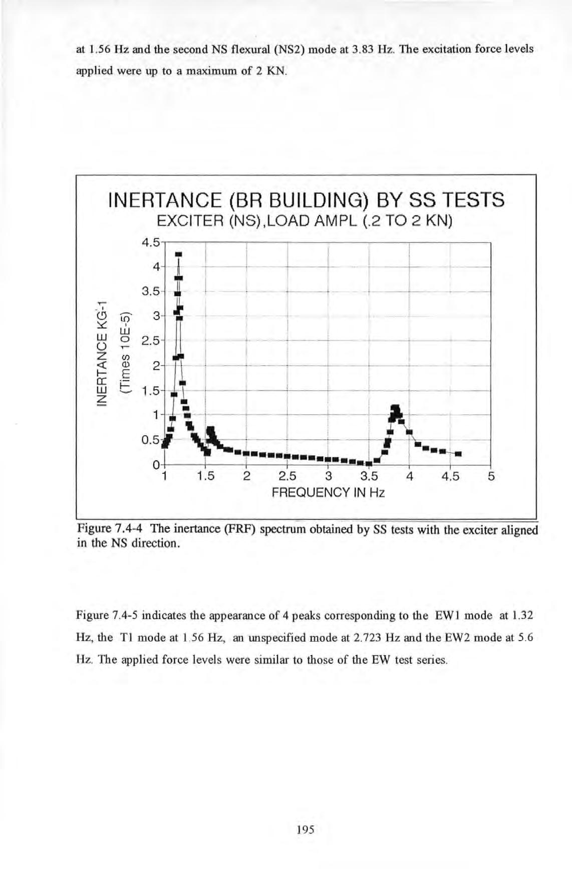
Figure
indicates the appearance of 4 peaks corresponding to the EW 1 mode at 1.32 Hz, the Tl mode at 1.56 Hz, an unspecified mode at 2.723 Hz and the EW2 mode at 5 .6 Hz. The applied force levels were similar to those of the EW test series
.,...... • I (!) w 0 z <{ f-a: w z
..--.. 1.{) I w 0 .,...... (/) Q) E f.= -I i · I ---i1 : __ .....____.;I ---· - ---- ---!---·' i - r ; j _j__.,... -, •· 1 5 I -:-----f1 ':---i . ; : - f. _;_ i i i • ! : • .. i ; :, , , o.5 . : . : --+-:- I -+'. - · ··- ' ' .·. Jll '.,1 ! ! • 1 1 5 2 2.5 3 3.5 4 FREQUENCY IN Hz 4.5 5
Figure 7.4-4 The inertance (FRF) spectrum obtainect by SS tests with the exciter aligned in the NS direction.
195
7.4-5
INERTANCE (BR BUilDING) BY SS TESTS EXCITER (EW),LOAD AMPL ( 4 TO 2 KN)
A typical time history record of the PRBS excitation force (load) and the resulting responses from the two accelerometers are also shown in Figure 7.4-6.
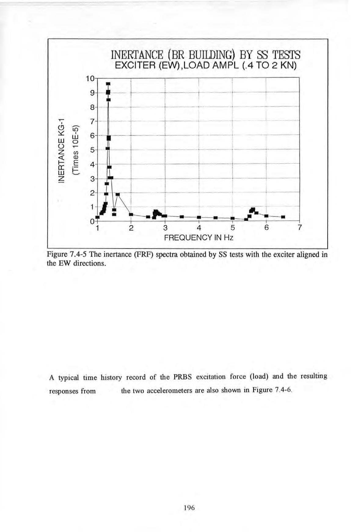
,.-I <.9 ......... l{) y: I w w 0 0 ,.-- 5 z (/) <( Cl> I- E 4 a: F w z 3 ---r------- r j ; f ·-·· ----------·- -t·------t--·----+----l ---+-----:- ; - 1 i I ' ; I -· i -·-t-------t---r-i 1 i l --f------- · t I' 7
Figure 7.4-5 The inertance (FRF) spectra obtained by SS tests with the exciter aligned in the EW directions.
196

I _ l-:· I ' f I _. ! I·· I --... t -!... -- -t.:: r1 l I i - - - t- · - I -· • +- r- --·· i·· : ·· . r · 1 -·· · I -1 - ··_ ·l .lr i ,j}- . i I :- .. 1- i lf l I J1 n ' f\ · .. - 11 · ,. -NfiJ \ W - : ]-_ il vTI ;J : -- ; ... - i 'IV ! I i \-._. ' -- · \ •••• ! I \1 - u : .h._ !_ h - -H+ -+--t-_1-Lt-t-- 11 I roJ - ! I V -V ; ! j : i 1 - ;-' -; - · : ; -:-:·..... I - i lt ! I I • , - -'-- - -r --·· . -1-·- r---+-+----'1-+--1 I r • · · - · I : I ; I·+ . .-r· I ' i. I.I I t , I I I ! I I , ri - - I I I : : I l ; : : 1 1 res ponse from the two accelerometers ; -. l l ·-- - !=- --t --1- -: ' __,____ __t__ -· r- l i • : , : 1-t- - I , : -- r-:- I . . - f-- I ! I ; - I 11.. : . I -1!- I - , - i ' : 1\ · - : · · · t · '\ -1-- - '-- - - ,- f- c---- - II , I --- ·---4 --L ; • • I - -!- !-I · • t- r-- -1-- l I r 1 --+-I 1 ! I i- - - ! ! ., - 1-_ .I -L ··- . . : _- i .. .. : : 1 I 1 t . ,.. t- - 1- t- ·r--.- : ·=- :-- - excitation force :· t-t- 1• 1, _.. 1 • i I ,.__ : i -l · IX !_ -r-- -1tii;A "" ...,f i1'"·prr V!! - :- - - - 1-· j- -, j- - i _._ · -1----+---+---+---t--+--+- -- I --. ..L ! -. . . - - - 1- l --· - !- r - I - -r-- t- - - -r-- =----- --=- r 1-- -1--:·=:= - --+ + - -.--- -- i- - 1- 1- -_ 1- - -·:- I -- --- -1-- - · -
197
Figures 7 .4-6. A typical time history record of the PRBS excitation force (load) and the resulting responses from _ the two accelerometers
The exemplary values of the resonance frequencies of the various modes are summarized in Table 7.4-1. TABLE 7.4-l. THE TABLE OF EXEMPLARY VALUES OF THE RESONANCE FREQUENCIES OF THE VARIOUS MODES OF THE BR BUILDING.
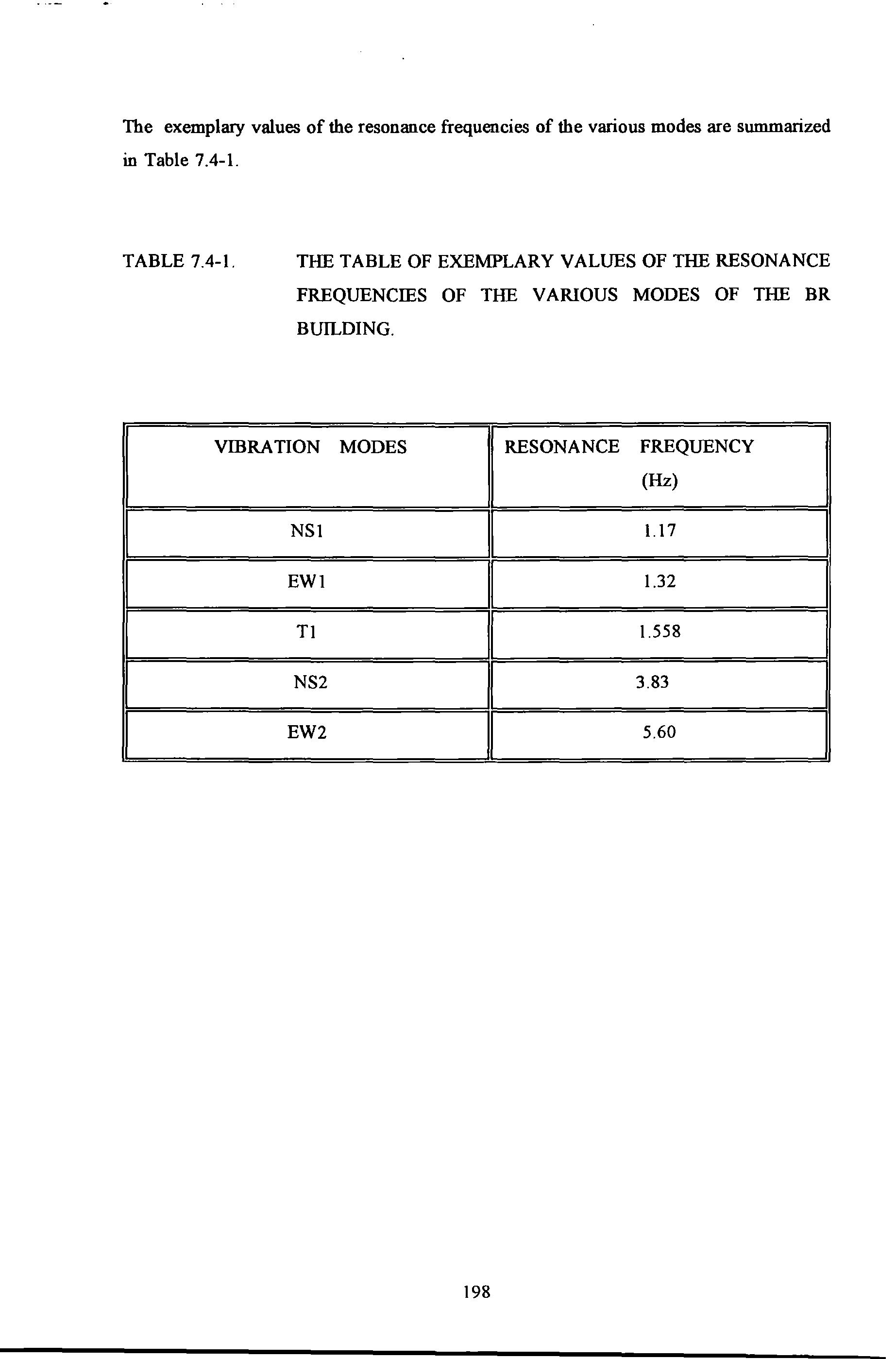
VIBRATION MODES RESONANCE FREQUENCY (Hz) NSl l.l7 EWl 1.32 Tl 1.558 NS2 3.83 EW2 5.60 198
Figure 7 4-7 show the mode shapes of the NS 1 mode as determined from the SS and PRBS tests (the annotations in the figures are: 1ACT-EW 1 denotes the actuator was in EW
1230486 1 denotes the date of the and so on) The SS test was performed with the exciter acting in the NS direction . Whereas the PRBS test was performed two days after the SS tests with the exciter acting in the EW direction . The two curves obtained are in general agreement except that a spurious data point was obtained with the latter. It has to be borne in mind that the SS tests were of much larger forcing amplitudes than the PRBS count erpart. So the discrepancy, though small, might be due to changes in the behavioural mechanism of the structure in addition to the normaJ measurement errors.
NORMALIZED VALUE

LEVEL 1 - S INE,ACT-NS,230486 1 ; --+- PRBS,ACT-EW,250486 I
FLOOR
199
Figure 7.4-7 The NS 1 mode shapes determined from the SS and PRBS tests .
By plotting the NSl mode shapes obtained from this experiment alongside those experimental data reported by Williams (uJ, and those recommended by CIRIA (? IJ and ESDU 12 48 • 2 49 • l joJ as in Figure 7.4-8 , it is noted that the linear mode and the CIRIA recommended mode shape are close approximations to the one measured.

40 30 HEIGHT OF FLOOR LEVEL (m) 10 0 NORMALIZED VALUE
-TSANG ---+- WILLIAMS ---7tE- C IRIA
-a--- CIRINES DU LINEAR
200
Figure 7.4-8. An overlaid plot of the NSl mode shapes obtained from this experiment and other recommendations
Figure 7
shows the mode shapes of the EWl mode determined from the SS and the PRBS tests performed on different dates. The exciter was aligned in the EW direction in all these cases and the three curves obtained are in excellent agreement This indicates the credential of the test data and that tests results are repeatable over a period of time.

FLOOR LEVEL 0 NORMALIZED VALUE
.4-9
SINE,ACT-EW1704 --+- SINE,ACT-EW,2204 - PRBS,ACT-EW
201
Figure 7.4-9 The mode shapes of the EWI mode determined from SS and PRBS tests performed on different dates.
Again the EWl mode shape obtained from this experiment is plotted alongside the other recommendations annotated in Figure 7.4-10 Once again , the linear and the CIRIA recommended mode shapes seem closer approximations to the one measured
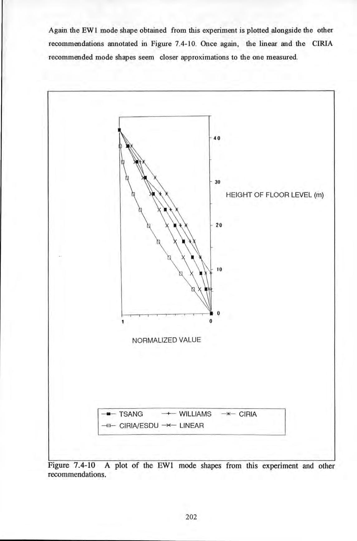
HEIGHT OF FLOOR LEVEL (m) 0
NORMALIZED VALUE
- TSANG --+- WILLIAMS ---*'- CIRIA --e- CIRINESDU LINEAR
202
Figure 7.4-10 A plot of the EWl mode shapes from this experiment and other recommendations.
Modes shapes corresponding to the modes Tl is given in Figure 7.4-ll. The results from the PRBS and the SS tests , with the exciter aligned in the EW direction in both cases, are consistent and in good agreement except an occurrence of a spurious data point at the 4th floor level. However, results from the SS tests , with the exciter aligned in the NS direction , produced somewhat different results from those obtained in the EW direction .
MODE SHAPES OF 1ST TORSIONAL (1 .558 HZ) FOR THE BRITISH RAIL BUILDING, PLYMOUTH

1 0 ···························-:-················ ········-·· :··············· ··· ·-···· -:-··· ··········· ···················································r ················ FLOOR LEVEL '-·· ····· 5 ····························• ················· ········r· · NORMALIZED VALUE 0 -
--+--
SINE,ACT-EW,2204
SINE,ACT-NS,2304 - PRBS,ACT-EW
203
Figure 7.4-11 Modes shapes of the Tl mode.
The NS2 mode is given in Figure 7.4-12 The figure shows that the node of this mode is close to the 8th floor level.
MODE SHAPE OF 2nd NS MODE (3.83 Hz) FOR THE BRITISH RAIL BUILDING, PLYMOUTH

FLOOR LEVEL ---- ···----··----- ' -·----- ·-----·--···· ·--- - 2 ·1 0 1 NORMALI ZED VALUE
204
Figure 7.4-12. The NS2 mode.
The EW2 mode shapes determined from 3 different experiments are also given in Figure 7.4-13 . Again good agreement is obtained. The node of the EW2 mode is shown to lay between the Sib and 91h floor levels .
MODE SHAPES OF 2nd EW (5.6 HZ) FOR THE BRITISH RAIL BUILDING, PLYMOUTH
NORMALIZED VALUE

FLOOR LEVEL
- SINE,ACT-EW,
SINE,ACT-EW,2204 PRBS,ACT-EW,2504
1704
205
Figure 7.4-13 The EW2 mode shapes detennined from 3 different tests.
The task of modelling the building is potentially a difficult one because of the numerous structural connections involved in articulating various structural members :beams, columns, shear cores, shafts, infilled walls, cladding etc. Also these structural members are mainly made of inhomogenous materials such as reinforced concrete. Unlike other structural materials which are manufactured in a controlled factory condition, reinforced concretes are mixed and cured in-situ. The quality hence structural properties of these materials are difficult to maintain.

The shear cores and planar shear walls present another difficulty in modelling. Because of the high depth-to-span ratios, shear deformation of these structural elements are significant. Simple bending theories are inadequate and deep beam theories are more appropriate. In particular, the shear cores forming the lift shafts are thin wall open sections (therefore asymmetric) The open edges of the shafts are connected by thick lintel beams at each floor level. Because of asymmetry, shear centre do not coincide with geometric centre. Hence flexural bending of these elements are strongly coupled with torsion as well. Their interactions with the other elements are even more complex.
A finite element model of the BR building was constructed from simple beam elements. To reduce complexity, a number of assumptions were made.
a. The raft foundation and the soil stratum supporting the structure is assumed infinitely rigid so that full fixity of the base of the structure is assured and no translation or rocking of the foundation is allowed.
b. The structural joints between members are assumed fully rigid.
c. The horizontal elements such as the beams and floor slabs are assumed to have infinite in-plane and out-of-plane bending stiffness.
The fmite element model was constructed usmg P AFEC on a main-frame PRIME computer. Figure 7.5-1 shows the wire-framed finite element model of the structure. There are over 300 nodes and 900 members in the model. The computations required quite extensive computer resources to complete. In constructing the model, simple ID bending
7.5 ANALYTICAL
OF THE BR BUO...DING
MODEL
206
beam elements were used for columns and beams and 1D shear beam elements were used for shear walls and cores. Very large moment of inertia values were used for the horizontal elements to assure the inftnite stiffness assumption was met. These values were taken typically as 1000 times that of the maximum of the vertical ones. Figures 7.5-2 to 7 .5- 4 show the mode shape of the EWl , Tl and the EW2 modes

.,, I 7 7 17 I • -----v'i / 71 / 1 .I y 7 7 / 1 / · I ·· I L__j/ , _J,,/ ---;- / VI I / I 1 /
2 07
Figure 7 5- 1 The wire-frame finite element model of the BR Building
 Figure 7 .5-2a
208
A 3 dimensional perspective view of the EW 1 mode from the finite element model of the BR building .

-
,
Figure 7 5-2b
A side view of the EWl mode from the finite element model of the BR building
209
Figure 7.5-3a A 3 dimensional perspective view of the T l mode from the fm1te element mode l of the BR building
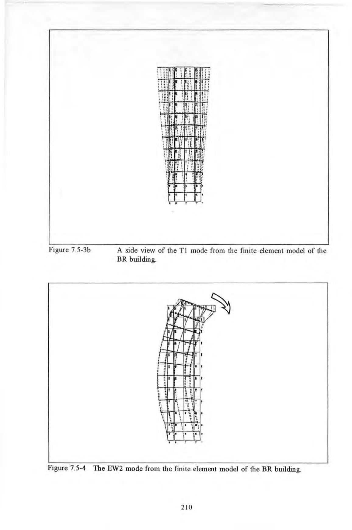
I jc 1 po I I a. !"
Figure 7 5-3b
A side view of the Tl mode from the finite element model of the BR building.
2 10
Figure 7.5-4 The EW2 mode from the finite element model of the BR building.
COMPARISONS OF EXPERIMENTAL AND ANALYTICAL RESULTS
The resonance frequencies of the modes determined from the experiment and the undamped natural frequencies from the fmite element model are summarized in Table 7.6-l. TABLE 7.6-l.
THE TABLE OF COMPARISON OF THE VALUES OF THE RESONANCE FREQUENCIES OF THE VARIOUS MODES FROM EXPERIMENTS AND THE UNDAMPED NATURAL FREQUENCIES FROM THE FINITE ELEMENT MODEL.
Generally speaking, both the frequency values and the mode shapes obtained via the experimental and analytical means are in broad agreement. There are some interesting observations to be gleaned from these results. Firstly, all the mode shapes show that the floors remain planar as anticipated from the assumptions made. Secondly, the values of the natural frequencies of all the modes from the finite element model are as higher than the corresponding experimental ones. This is possibly a direct result of the over-stiff horizontal elements assumed. Thirdly, the mode shape of EW 1 is very close to the straight line approximation as suggested by Jeary and Sparks 11.391 and reviewed in Section 2.1.2.3. Finally, the node of the EW2 mode in the fmite element model occurs between the 81h and the 91h Floor which agrees with its experimental counterpart.

7.6
VIBRATION NS1
EW1 Tl EW2
I
EXPERIMENTAL
MODES RESONANCE UNDAMPED FREQUENCY NATURAL FREQUENCY (Hz) (Hz) 1.17 I 1.112 1.32 I 1.481 1.558 I 3.289 5.60 6.455
FINITE ELEMENT
211
Ambient vibration test technique has rather limited value as far as identification is concerned because the input excitation cannot be measured. Generally, the measured signals (acceleration response) were noisy as reflected by having very low values in the coherence spectra obtained from the experiments carried out. Identifying the appearance of a mode using the criteria of a peak in the autospectra of response is not conclusive. Also very long recording time is required to improve confidence levels of random signals. During the long hours of measurement, undue disturbance can happen and cause disruptive effect as far as accuracy is concerned.
Exciter-induced vibration test usmg a SS or PRBS forcing functions is more useful. However, the level of response obtained may not be as high as its ambient counterparts. SS test is in general very time intensive. The PRBS test is a better technique for field testing as far as the time saving is concerned. With good care in carrying out the signal processing : sampling, filtering, windowing, averaging etc, a PRBS test can produce very good results. This was reflected by the higher values in the coherence spectra obtained from the experiments carried out.

For common building structures, the natural frequencies and mode shapes recommended by the various design literature are close approximations to the experimental ones. They can be used as estimates if no other experimental data is available.
The FE modelling of the BR building carried out was very demanding on the computing resources in carrying out the calculations and producing the analytical results. In general, the undamped natural frequencies from the FE models are close to but consistently higher than the experimental ones. However, the order of occurence of the analytical modes (in ascending order of their natural frequency values) are the same as the experimental ones.
7.7 SUMMARY
212
CHAPTER 8
FULL SCALE FORCED VffiRA TION TESTS OF A FIRE STATION DRILL TOWER
8.1 INTRODUCTION
This chapter reports the results of full scale forced vibration tests conducted on a six storey fire station drill tower. These tests were similar in many respects to those reported in chapter 7 except that the size of this structure was much smaller and more extensive measurements were carried out with the use of the CAT described in Chapter 4. Also much larger amplitudes of response were obtained using the same shaker.

8.2 DESCRIPTION OF THE STRUCTURE
The tower is situated at Camel's Head Fire Station, Plymouth and used for fue fighting training. This structure is simpler in structural form when compared to the BR building but accurate structural modelling of this structure is by no means a trivial task. Structurally, it can be treated as a reinforced concrete frame with most openings partly inftlled with brick walls. The uncertainty regarding the interactions between these walls and the frame accounts for some of the modelling difficulties. Figure 8.2-1 gives a photographic view of the structure.
213
8.3 TEST ARRANGEMENTS AND PROCEDURES

Again the exciter was located as high up on the structure as possible In this case, the exciter and the test equipment was placed on the fifth floor. The exciter was secured on the floor slab using the same technique as those used in the BR building Because of very restrictive access, there were considerable difficulties in getting the equipment to this level. Eventually, this problem was overcome with the use of a fire-fighting hydraulic platform, courtesy of the Devon and Cornwall Fire Service.
Mains electrical power in the tower could only be obtained from the power points in the nearby station via very long extension cables. Voltage drop and power loss caused some difficulties in operating the electrical equipment. Furthermore, the weather condition was at times very undesirable. Temporary shelter had to be provided to protect the equipment from damage This, once again, highlights the difficult circumstances encountered in field testing not normally found in laboratory testing .
I .___ .. - -·; ··, ·. . ..
Figure 8 2-1
A distant photographic vtew of the Camel's Head Fire Drill Tower, Plymouth
214
The location of the exciter is shown in Figure 8 3-1 Two test series were carried out, each with the exciter orientated in either one of the two principal axes These two directions are designated as EW and NS as shown in Figure 8 3-1

Acceleration response of the structure was measured at a set of pre-determined points. The horizontal positions of the four grid points are designated as A 1, A2 , B 1 and B2 , as shown in Figure 8 3-1 These arrangement of points repeated themselves for each of the floor level. An encoding system was used such that a point designated as OA2 is referred as the point A2 on the ground level and so on .
8.3-1 Location of the exciter and designation of the grid points.
Three roving accelerometers were positioned at each of the measuring locations : two accelerometers were aligned with their sensitivity axes horizontally along the EW and NS directions respectively , while the third one was aligned vertically . This arrangement enabled a measurement of the spatial translations of each of the twenty -four points . A reference accelerometer was fixed at one location, in this case at SA I , to allow the plotting of operating shapes using the traditional technique (reported in Chapter 7).
N Al E
BALCONY ,.._REINFORCED
Bl
BRICK WALL
CONCRETE COLUMNS
Figure
2 15
The inertance and transmissibility measurements were obtained from tests carried out using Pseudo-Random-Binary-Sequence (PRBS) and Step-Sine (SS) excitation. As before, the SS tests with fine steps were only carried out for locating the resonance frequencies of the modes. The bulk of the inertance and transmissibility FRF measurements were taken using PRBS excitation. The spectrum analyzer used was set in the 25 Hz baseband when taking these measurements. This setting provided a frequency resolution of 0.2 Hz. A limited number of zoom measurements with a 0.04 Hz resolution were also taken. Inertance measurements were taken to provide data for modal parameter determination. Transmissibility measurements were taken to determine the operating shapes of the tower under the action of the shaker and at each of the tested frequencies.
Each test was encoded by a Test-Identification (TI) code which provide a unique reference to the location of measurement and other relevant test conditions. A schedule detailing the various test runs and the corresponding TI codes is given in Appendix 8.3.
8.4 TEST RESULTS
The success of incorporating the CAT produced a large collection of data which required quite elaborate data processing efforts involving desk-top PC as well as an IBM main frame computer. Only a representative sample of the results of this analysis is presented below. The results from the SS tests are given first and followed by those from the zoom PRBS tests. The results of the modal parameters determined using data from the 25 Hz baseband are also given.

Figures 8.4-l to 8.4-5 show the typical modulus and phase inertance FRF plots obtained using the SS tests with small-steps. These test data were obtained with the exciter aligned in the EW direction and response measured at point SAl.
In Figure 8.4-l, two very close peaks at frequencies 2.34 and 2.48 Hz (a mere 0.14 Hz gap between them) and other peaks at 5.4 and I 0.3 Hz are detected. It is also noted that these peaks correspond to a 90 degree phase change at each of the corresponding peaks' frequencies.
216
The changes of inertance and acceleration response levels with the increase in levels of excitation force at the two frequencies 2.34 and 2.48 Hz were determined and plotted in Figures 8.4-2a to 8.4-2b
Each of the Figures 8.4-3a to 8.4-3c show a peak at frequency around 5 52, 5 56 and 5.4 Hz when excitation force amplitudes were 0 .05 , 0 . 10 and 0.15 KN (r.m .s) and the corresponding acceleration response amplitudes were 2,4 and 5 milli-g (r m s ) respectively (Note 1 g = 9 807 m/s2 ) In other word s, the frequencies corresponding to the peaks fluctuate as force amplitudes change

---. -··
7.00E-04 .-----:o:-----------------.- 180 6 00E-04 160 r-i J, 5.00E-04 . w 4.00E-04 u 3.00E-04 2.00E-04 l.OOE- 04 140 r>:l 120 0 r>:l 100 A 80 r>:l 60 40 :I: r P-. 20 OOOE+OO 0 0.0 2.0 4 0 6.0 8.0 10.0 12.0 FREQUENCY IN Hz 1-
FIRE TOWER INERTANC E ,PHASE FRF ACT( EW) ,ACC(SA 1)
INERTANCE-+- PHASE
Fig ure 8.4-1 Modulus Inertance FRF plot using SS tests .
2 17

FIRE TOWER RESPONSE Vs LOAD LEVEL ACT (EW), ACC (5A1), FREQ=2.34 Hz •' · 0.04 0.04 5.20E- 04 I 5.00E--Q4 () '··.._.____ N 0.04 w 4.BOE- 04 u 4.60E- 04 11: 4.40E--D4 4.20E- 0 4 0 03 0.03 0.03 0.03 0.03 0.02 / 4.00E- 04 0 02 0.0 4 0.05 0.06 0.07 0.08 0.09 0.10 LOAD IN KN 1--- INERTANCE -+--- ACCELRATION s z 0 w u u <t
FIRE TOWER RESPONSE
LOAD LEVEL ACT (EW), ACC (5A1) , FREQ=2.48 Hz 3.40E--D4 / 0 06 3.30E- 04 0 05 C\1 {/) I3.20E- 04 0 05 8 () I 0 04 z w 3.10E-04 0 u t:: 3.0 0 E-04 0 04 < • 2.90E-04 J 0 03 w u u 0.03 < 2. BOE-Q4 2.70E--D4 0 02 0 06 OOB 0 10 0 12 0.14 0 16 0.18 LOAD IN KN 1- INERTANCE
ACCELRATION
Figure 8.4-2a Change of acceleration and inertance of the mode at 2.34 Hz with increase magnitude of force using SS excitation.
Vs
-+---
2 18
Figure 8.4-2b Change of acceleration and inertance of the mode at 2.48 Hz with increase magnitude of force using SS excitation
and phase inertance FRF plot using SS excitation. Measurement was made at SAl with exciter acti ng in the EW direction and force

... FIRE TOWER INERTANCE, PHASE FRF ACT (EW), ACC {5A1), 220487 4.00E-04 160 00 3.50E-04 140.00 120.00 I 0 3 00E-04 Ill 10 0.00 2.50E-04 80 00 I f-< I ffi 2.00E-04 / /" 60.00 ' 1.50E-Q4 40.00 l.OO E-04 20.00 5.40 5.42 5.4 4 5.46 5.48 5.50 5 52 5 54 5.56 5.58 5.60 FREQUENCY IN Hz 1 - IN ERTANCE FRF PHASE FRF Ill Ill 0 Ill Ill ::r: p..
amplitudes
OS K.N (r.m.s ) FIRE TOW ER INERTANCE, PHASE FRF ACT (EW), ACC (5A1) , %C=500 3.50E-04 I 3.00E-04 0 w 2.50E-04 u 2.0 0E- 04 l. 50E-04 l. OOE- 04 160.00 140.00 120.00 100.00 80.00 60.00 40.00 20 00 5. 00 E-05 0.00 5 35 5.40 5.45 5.50 5.55 5 60 5.65 5.7 0 5.75 FREQUENCY IN Hz 1-- INERTANCE FRF -+- PHASE FRF Ill Ill 0 l>l l>l ::r: p..
Figure 8.4-3a Modulus
of O
at
amplitudes
K.N (r m.s.) 2 19
Figure 8.4-3b Modulus and phase inertance FRF plot using SS excitation. Measurement was made
SAl with exciter acting in the EW direction and force
of 0.1
FIRE TOWER INERTANCE, PHASE FRF
Figure 8.4-3c Modulus and phase inertance FRF plot using SS excitation. Measurement was made at SAl with exciter acting in the EW direction and force amplitudes of 0 .15 KN (r.m.s.)
Figure 8.4-4 shows a peak at 10.48 Hz With the exciter acting in the NS direction , the inertance FRF plots obtained are similar to those obtained from the EW direction as regarding the locations of the resonance peaks are concerned . Therefore, they are not to be shown here except the one plotted in Figure 8.4-5 .

ACT (EW), ACC (5A1), %C=900 3.50E-Q4 ......---- - ---.I 0 3.00E-Q4 lt: 2.50E- 0 4 w r. 2.00E-04 0: w l .50E- 04 · - -----.. l.OOE- 04 160.00 140.00 120.00 100 00 80.00 6 0.00 40 00 20.00 0.00 5 30 5 3 5 5 40 5 .45 5 50 5 55 5 60 5 65 5 7 0 5.75 FREQUENCY IN Hz 1- INERTANCE FRF---+- PHASE FRF w 0 w 0 z w ll.
220
FRF plot of the mode at 10.48 Hz using SS excitation. Measurement was made at 5Al with exciter acting in the EW direction
-+----
I
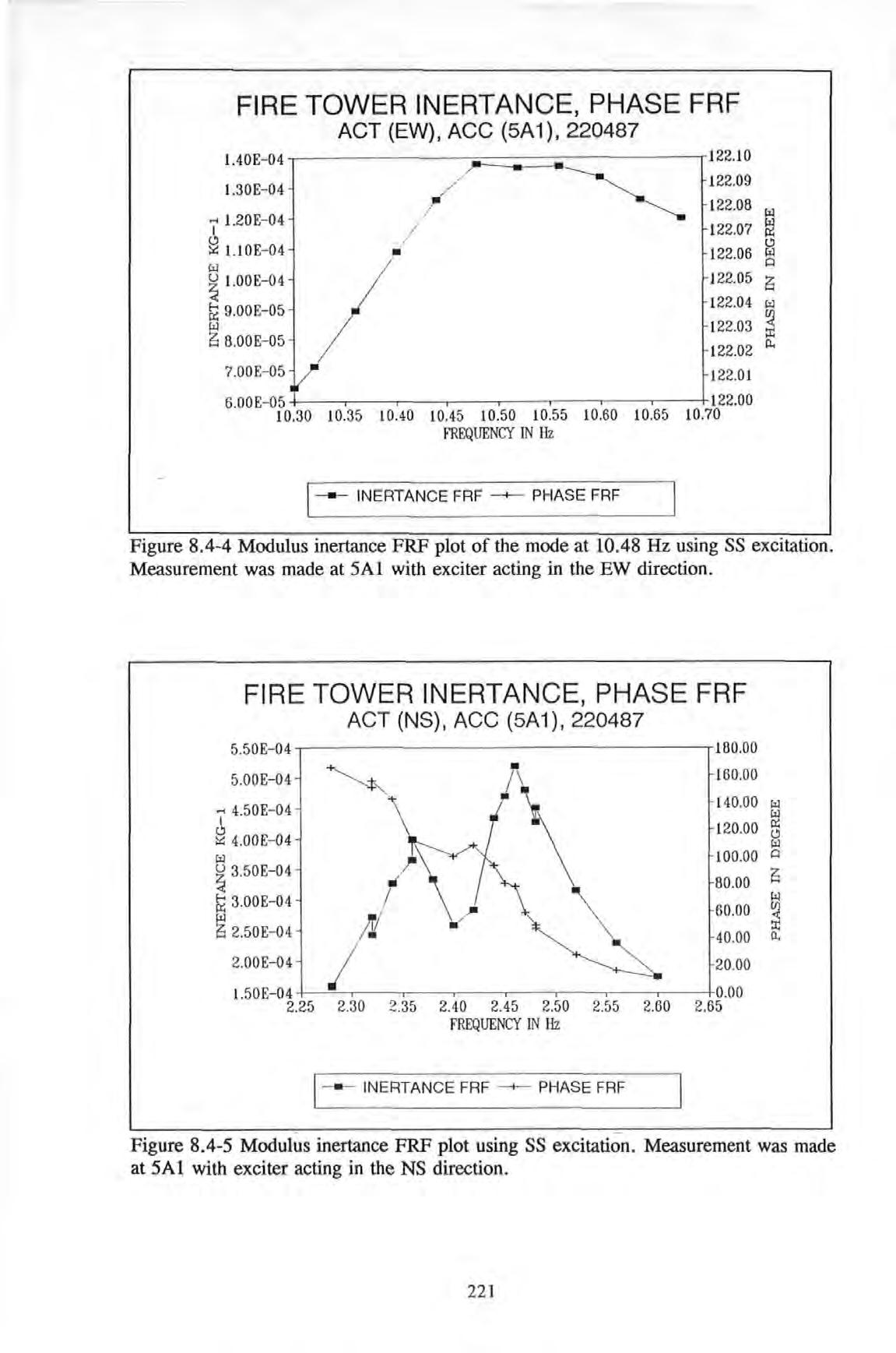
FIRE TOWER INERTANCE , PHASE FRF ACT (EW), ACC (5A1), 220487 122.10 l.30E-04 1.2 0E-04 I g l.lOE-04 w l.OOE-04 9.00E-05 8 00E-05 7.00E-05 • 122.09 122.08 / 122.07 122.06 122.05 122.04 122.03 122.02 122.0 1 122. 00 6.0 0 E-05 +----.------.-----.----.------.----.------.----+ 10.30 10.35 10.40 10.45 10.50 10.55 10 .60 10.65 10.70 FREQUENCY IN Hz 1-- INERTANCE FRF -+---- PHASE FRF l:zl !)! l!l l:zl Q 2; l:zl ::c 11.
FIRE TOWER INERTANCE, PHASE FRF ACT (NS), ACC (5A1), 220487 5.50E-04 180.00 • 160 00 5.00E-04 j\ ,.... 4.50E-04 \ \ 140.00 I 120.00 4.00E-0 4 l:zl 100.00 3.50E-04 80.00 3.00E-04 l:zl 60.00 2; 2.5 0E-04 40.00 2. 00 E-04 I 20 00 1.50E-04 0.00 2 25 2.30 2.35 2.40 2.45 2.50 2.55 2.6 0 2.65 FREQUENCY IN Hz 1- INERTANCE FRF
PHASE
l:zl l!l l:zl Q z l:zl n..
Figure 8.4-4 Modulus inertance
FRF
22 1
Figure 8.4-5 Modulus i nertance FRF plot using SS excitation. Measurement was made at 5Al with exciter acting in the NS direction .
Figure 8.4-5 shows again two very close peaks at 2.36 and 2.46 Hz. This observation agrees with those obtained by the EW excitation. Indeed, the results from the zoom analysis (with a resolution of 0.04 Hz) suggest that there are actually two very close modes: one with a natural frequency at 2.328 Hz and the other at 2.416 Hz (as identified by the algorithm). It is not just the one peak as appeared in all the other measurements taken with a 0.2 Hz resolution. It is clear that the 0.2 Hz resolution, used in the PRBS tests, is not fme enough. However, this is considered a necessary trade-off between resolution and time needed for taking measurements. This 25 Hz baseband setting is necessary in order that all the required measurements can be completed within the short time allowed.
Figures 8.4-6a to 8.4-6c show the inertance FRF spectra taken from the zoom measurements at SAl, with centre frequencies fixed at 2, 5 and 10Hz respectively. In these tests, the exciter was orientated in the EW direction. The corresponding phase inertance spectra are also plotted between 0 and 360 degrees as shown. The results of the analysis are also summarized in Table 8.4-1.

222

0 0 ::-! 3 15 f'requenoy In h•
0 : 3 ._ s e 7 ._ .5 e 7 f'r•quenoy In h•
Figure 8.4-6a Inertance FRF spectra from PRBS (EW) test (TI R2304007) zooming in at 2Hz.
: 12 t l e D 10 11 12
Figure 8.4-6b Inertance FRF spectra from PRBS (EW) test (TI R2204006) zooming in at 5Hz
223
Figure 8.4-6c Inertance FRF spectra f rom PRBS (EW) test (TI R2304003) zooming in at 10 H z .
Table 8.4-1: ZOOM ANALYSIS WITH A RESOLUTION OF 0 04 HZ (EW EXCITATION)

Data from the tests R2304007 and R2304001 were obtained with the attenuator dial set at 1000 and 300 ( %C values) respectively . The %C values are readings on the 10-turns attenuator dial in the DARTEC control panel. This dial attenuates the input driving signal fed to the control panel. A %C value of 1000 denotes zero attenuation and a %C value of 0 denotes full attenuation .
The modal parameter analysis carried out was able to identify the two very close modes as given in Table 8.4-1. It appears, at least based on these results , that at higher force level (i e higher %C setting), resonance frequencies and modal damping factors of the two modes change slightly but the magnitudes of the change are considered to be too small to conclude any trend
The tests R2204005, R2204006 , R2204008 and R2304002 are all able to identify the Tl mode Results based on these data have al so indicated the change of modal parameters at different force levels . Again , the change in values are considered to be too small to speculate any particular trend at all.
TEST RUN NATURAL DAMPING MODAL MODE NOTE TI FREQ CONST (Hz) (Kg-1) R2304007 2.333 1.478e- 2 1.887e-5 EWI %C=l000 R2304007 2 .429 9 045e-3 8 829e-6 NSI %C = l000 R2304001 2.311 1 503e-2 1 598e-5 EWI %C=300 R2304001 2.408 9 .064e-3 7 .06le-6 NSI %C =300 R2204005 5.597 1.258e-2 9.333e-6 Tl NA R2204006 5 .581 1.36le-2 1.1 18e-5 TI %C=300 R2204008 5.528 1.272e-2 9.400e-6 TI %C =700 R2304002 5 .578 1.305e-2 9.505e-6 Tl NA R2304003 10 51 1.38le-2 4.444e- 6 EW2 NA
22 4
Similarly, Figures 8 4-7a to 8.4-7e show the inertance FRF spectra from the zoom measurements taken at 5Al with centre frequencies set at 2, 5, 10, 17 and 25 Hz respectively In these tests, the exciter was acting in the NS direction
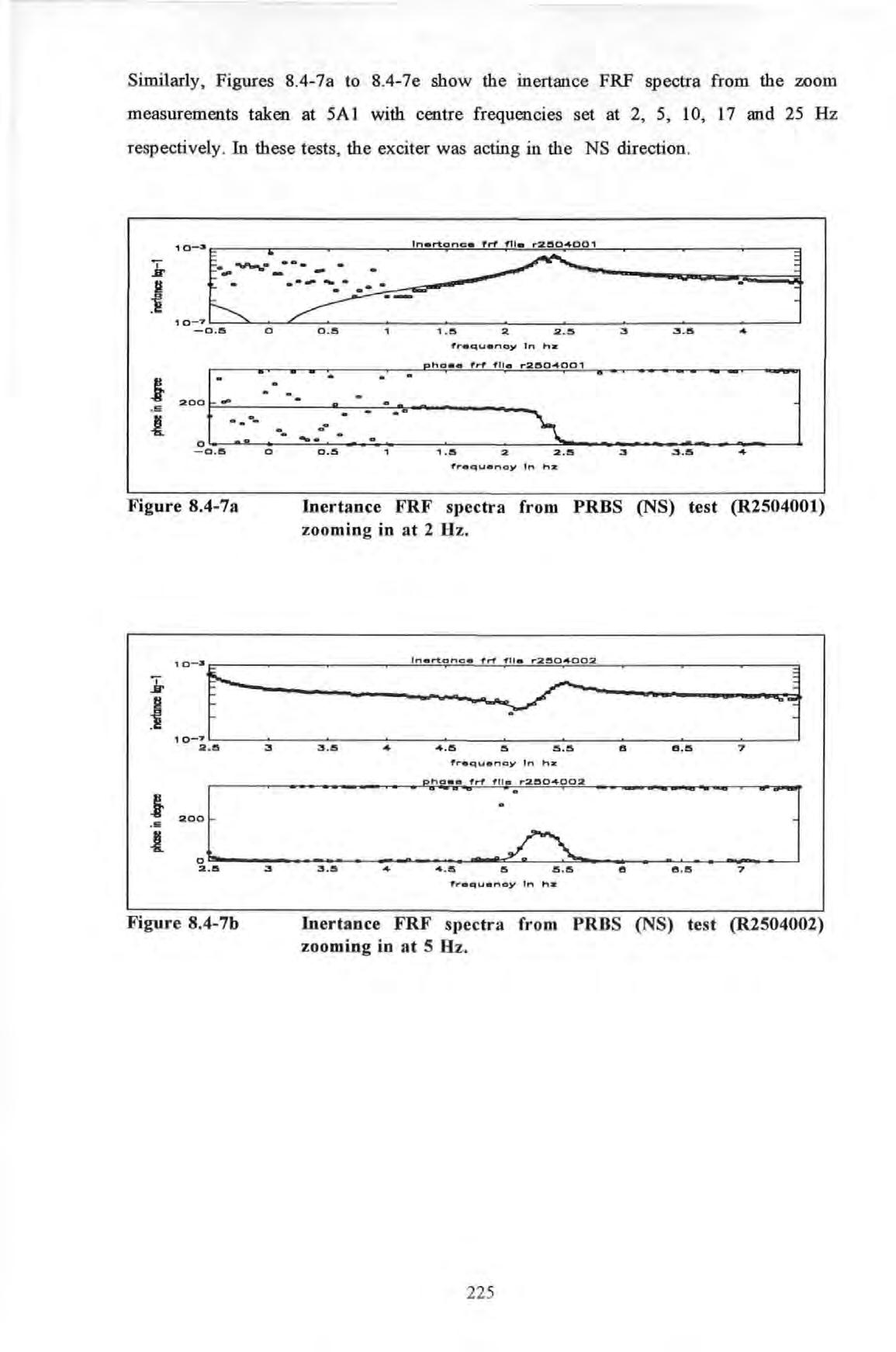
• : ·= -0 .15 0 0.15 , , 15 2. 2 .5 3 3.15 4 f'r•-=-u•nay In hz i ·J-......·:-.. ·. _..· "'.· ·;:• • : -0.15 0 0.15 , , 15 2 2.15 3
f'requoncy In hz
Figure 8.4-7a
frequency In hx •o:l fr"•quenoy In nz
Inertance FRF spectra from PRBS (NS) test (R2504001) zooming in at 2 Hz.
Figure 8 .4-7b
225
Inertance FRF spectra from PRBS (NS) test (R2504002) zooming in at 5 Hz.

(] ; ; : : :- : 1 7 .s e a s " D l5 1 o 1 o.l5 1 1 1 1 15 1 2 tn hz 7 s e a s o o l5 1 o 1 o.l5 1 1 1 1 15 1 2
Figure 8.4-7c
f',.equenoy t n hz
14.!5 115 1!5 !5 16 18 !5 17 17 15 1 8 1 6 !5 1D 14.!5 1!S 1!5.!5 1 e 1e s 17 17.!5 1 e 1 e !S o
Inertance FRF spectra from PRBS (NS) test (R2504003) zooming in at 10 Hz.
Figure 8.4-7d
Figure 8.4-7e
Inertance FRF spectra from PRBS (NS) test (R2504004) zooming in at 17 Hz.
'f"r•quenoy In hz
22 6
Inertance FRF spectra from PRBS (NS) test (R2504005) zooming in at 25 Hz.
The results of the analysis using these data are summarized in Table 8.4-2
In all , the results f ro m the zoom measurements show that very good agreement between the experimental and regenerated curves is able to obtain in al l the cases shown . This is due to the 5 times enhancement in the resolution: from 0 .2 to 0.04 Hz. Curves plotted with circles and solid curve denote the experimental and regenerated curves respectively so that the two curves do not obscure each other when overlaid

TEST RUN NATURAL DAMPING MODAL MODE FREQ CONST TI w , G, (Hz) (Kg -1) R2504001 2 328 1.730E-002 1.463E-005 EW1 R2504001 2.4 151 8.614E-003 8.903£-0 06 NS1 R2504002 2.443 1.451E-002 1.869E-005 NSl R2504002 5.496 1.315E-002 3 . 132E-006 T1 R2504003 10.470 1.453E- 002 2 .208E-006 EW2 R2504003 11.797 2 9 70 E-002 2 847E-006 NS2 R2504004 17.55 9 149E-003 1.222E-006 T2 R2504005 24.769 1 172E- 002 4 298E-00 6 NS3 R2504005 28 .138 7 .429E- 002 1.597E-005 unclassify
Table 8.4-2 : ZOOM ANALYSIS WITH A RESOLUTION OF 0.04 HZ (NS EXCITATION)
227
A small sample of the Inertance FRF spectra obtained are given below. All these spectra were taken in the 0 to 25 Hz baseband. Figures 8.4-8a and 8.4-8b show the modulus and phase spectra obtained from the grid point at 5A 1 while the shaker was aligned along the EW direction .

INERTANCE (FIRE TOWER) PRBS
RUN#220487001 R
PH AS E FRF (FIRE TOWER) PRBS
RUN#220487001 R
.... 6 0 0001 w () z a: w z
FREQUENCY IN Hz
180 (/) w w a: C) w 0 z 0 w .....1 C) z <{ -180 I 0
Figure 8.4-8a The modulus FRF spectra obtained from the grid point at 5Al while the shaker was aligned along the EW direction .
I I 10 15 20 FREQUENCY IN Hz ,_ 16 AVERAGES I 25
228
Figure 8.4-8b The phase FRF spectra obtained from the grid point at 5Al while th e shaker was aligned along the EW di rection.
Figure 8.4-8a shows that, in general, quite distinctive resonance peaks occur at frequencies b elow 17 Hz. But at higher frequencies, modes are heavily 'cramped' together. Because of the dense presences of modes, analyses carried out in the high frequency range will be difficult.
The typical procedures in carrying out the extraction process , using the algorithm/program described in Chapter 5 , is detailed below. First of all, the peaks in the Inertance modulus plot (the upper curve in Figure 8.4-9) were detected by visual inspection of the plot. A resonance mode is indicated by the occurrence of a peak in the modulus and the Imaginary Inertance p lot (the lower curve in Figure 8.4-9) The frequencies corresponding to each of the peaks were marked with a vertical line. Then the number of data points on either side of the marked frequencies were chosen for curve fitting . Because of the coarse frequency resolution in th e data , a small number of points was found to give better results . If too many points were chosen , it was more likely that some of these data points would render the ass umptions made in deriving the algorithm b eing violated A total of 7 modes were detected , analyzed and their associated modal parameters determined .

10- 3 1 ] 1Q- '7 20 1!10 eo 100 120 data point. x10-4 mark band• 1 2 1 0 20 1!10 eo 100 data point.
229
Figure 8.4-9 Marking resonant mode positions at the peaks in the Modulus or Imaginary Inertance FRF spectra.
The experimental and regenerated inertance FRF curves are plotted in Figure 8.4-l 0 for appraisal. Based on the data from the test R25X021X, a good correlation between the two curves is found , especially in the modulus plot. A close examination shows that although the phases near resonance are correctly determined, those near the anti-resonance regions (i .e. between consecutive peaks) are not. This is thought to be due to poor signal-to-noiseratio of measured signals in these regions.
Figure 8.4-11 shows the data and result from the test R25Y023Y (i.e. data taken at grid point 5B2 with the exciter and the accelerometer both aligned in the NS direction) . Again s imilar comments made for Figure 8.4-10 still apply . It is noticed that the phases measured between the peaks are quite erratic. This observation has reinforced the acute requirement for precise phas e measurement
 .,,..quenCUf rn ha
Figure 8.4-10 Inertance FRF spectra from PRBS test (R25X021X)
.,,..quenCUf rn ha
Figure 8.4-10 Inertance FRF spectra from PRBS test (R25X021X)
O •- •••nonoo M "'"i .J L: ;:& :; - ____;j m. ... 200. l 0 Figu•·e 8.4-11 15 10 15 20 2!5 15 frequency In nz 15 f',...quenoy In n11
230
Inertance FRF spectra from PRBS test (R25Y023Y)
Figure 8.4-12 show the data and result from the test R25Y021X (i .e . data taken at grid point 5A 1 with the exciter and the accelerometer both aligned in the EW direction)
Figure 8.4-13 show the data and result from test R25Y017Y (i .e . data taken at grid point 4A 1 with the exciter and the accelerometer both aligned in the NS direction)

!5 0 !5 20 2.5 frequency In hz
Figure 8.4-12 Inertance FRF spectra from PRBS test (R25Y021X)
frequency In hz •• X _.__a UW b i - :: . _____ -... 0 !5 20 2!5 In hz
23 1
Figure 8.4-13 Inertance FRF spectra from PRBS test (R25Y017Y)
Figure 8.4-14 show the data and result from the test R25Y001Z (i.e. data taken at grid point OA 1 with the exciter aligned in the NS direction and the accelerometer aligned in the Vertical direction) It is noted that even on the ground level, the vertical responses due to some of the lower frequency modes are still very prominent.
This curve-fitting procedure was repeated for all 144 inertance FRF spectra, each spectrum was similar to those exemplary spectra shown in Figures 8.4-10 to 8.4-14 . After considerable and arduous efforts , a ful l set of modal parameters was obtained A small extract of these results for a number of measurement points is given in Tables 8.4-3 to 8.411 at the end of this chapter.
In summary , the 2 36 Hz and 2.48 Hz modes cannot be properly resolved because the 0 2 Hz frequency resolution adopted in the test is inadequate. The natural frequencies and modal damping factors determined for each mode, from data obtained at different measuring lo cations, are generally in broad agreement but never identical as required by theory . This is in fact a common draw back of most SDOF methods . Because natural frequencies and modal damping factors are 'global' structural properties, they should be the same regardless of the location a measurement is taken . This property provide a useful criterion to cross check the quality of measurement data or the suitability of analysis methods. Judging from the data and the results obtained, both are deemed to have passed this check. In particular, the modal damping factors for the 5 modes determined are generally ranging between 1 to 4% which are well in lin e with the conventional damping values assumed for reinforced concrete structures.

f 15 , 0 , 15 :zo 215 frequency In hz 'frequeno)l In hz
Figure 8.4-14
Inertance FRF s pectra from PRBS test (R25Y001Z)
232
The exemplary values of the natural frequencies and modal damping factors of the fust 5 modes determined are summarized in Table 8.4-12

Table 8 4-12 The exemplary values of the natural frequencies and damping factors of the first 5 modes.
VIBRATION MODES
The complete set of modal parameters determined was used to plot the normalized normal mode shapes of each of the modes using the respective modal constant values (with due attention paid to their magnitudes and signs) at each measurement lo cation . A mode shape (in physical term) or an eigenvector (in mathematical term) is non-dimensional and can be scaled arbitrarily . Hence the r atio of the modal constants determined at any two arbitrary spatial points on the structure gives the same ratio of the mode shape coordinates of the respective eigenvector corresponding to their spatial positions .
The axes in the mode shape plots are designated as fo llo ws : XX for EW , YY for NS and ZZ for vertical The results determined f ro m the EW test series are presented first then followed by those determined from the NS test series . Figure 8.4-15a shows that this mode is predominantly a swaying EW 1 mode The 4 grid lines along the Z direction are essentially straight lines. The floor slabs remain essentially flat and movements of the four points on the ground are small but detectable.
NATURAL DAMPING FREQUENCY FACTORS Hz % EWl 2 34 1 2 to 2 2 NSI 2.48 1 2 to 2 2 Tl 5.35 0 7 to 2 7 EW2 10.30 1.6 to 4 6 NS2 11.70 2 3 to 7 8
233
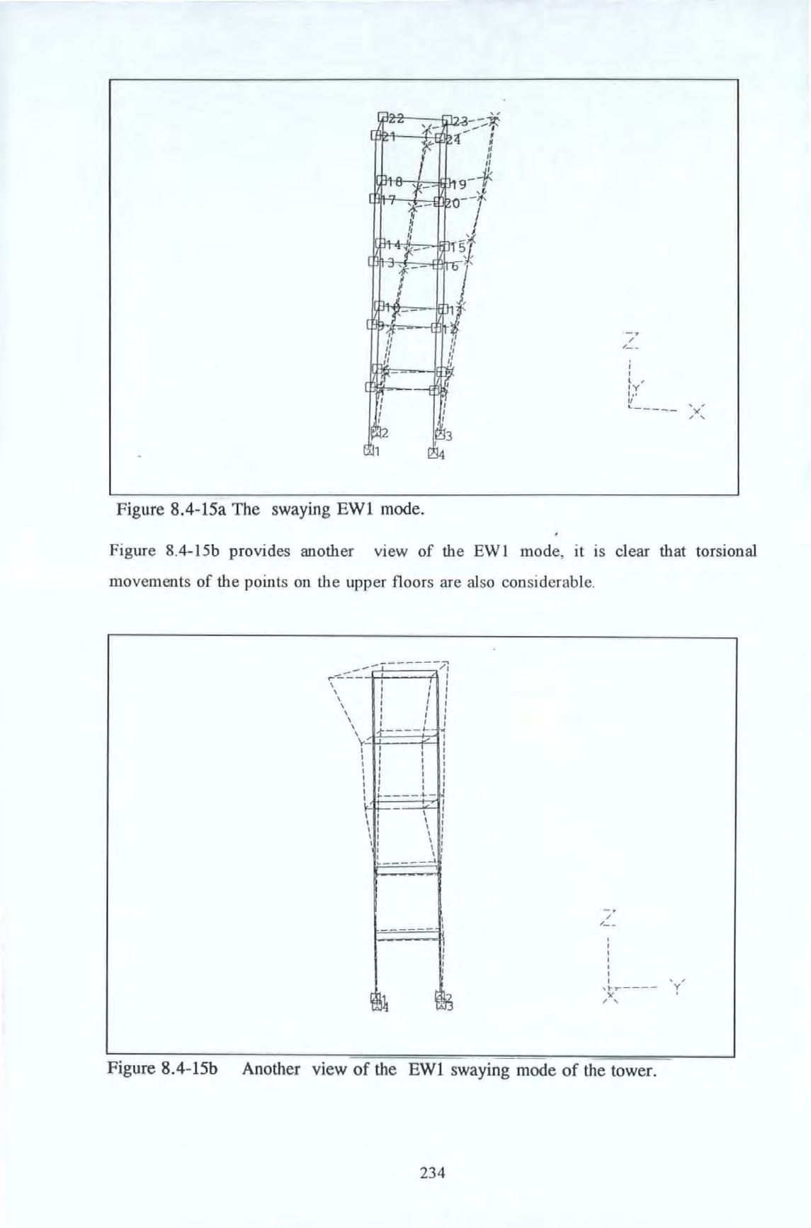
,.7__ I I ( , I Y lo• 11 _ ")(, / '
Figure 8.4-15a The swaying EWl mode.
Figure 8 4-15b provides another view of the EWI mode, it ts clear that torsional movements of the points on the upp er floors are al s o con si derable.
-\ ''\ \ \ \ \ -I I I I I I I I I I I I I -t----1/ I I I I I I I I I " y I I I I I I I I I I I I I I I I I I I I I I I I I I I I I I I ----+- i I \ I \ I \ I \ I I I I I \I \ I \I \ I I I I I I I - - I I I I I I IB\ / ' / _ I I I I I I I ... ... "' / '
Figure 8.4-15b
234 ' y '
Another view of the EWl swaying mode of the tower.
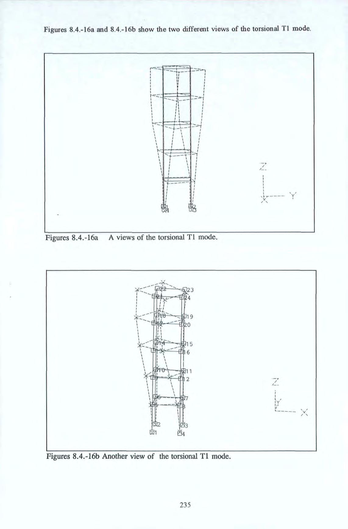 Figures 8.4 .-16a and 8.4.-16b show the two different views of the torsional Tl mode.
' t ' t t t t t I t t t t t ' t 1I t I I I I I "' I I I I I I I I - ------1"T-11 11 11 11 ' I---4--'• '• ''tt ..--.-+·- -+-'-I I I I I I I I I I I I '+---'T I I I I I I I I I I I I i-'''''' -:.-..., ' ' I '''''=-==i I ''''''' .::.::-t ''''''''"1 '''''''-,! ''''''
Figures 8.4.-16a
A views of the torsional Tl mode.
235 ' I I ' I I y 'S( / ' ' I l ' I Y l o• V __ ,)(, / '
Figures 8.4 .-16b Another view of the torsional Tl mode.
Figures 8.4 - 17 shows the EW2 mode in which a degree of torsional motion is also noted
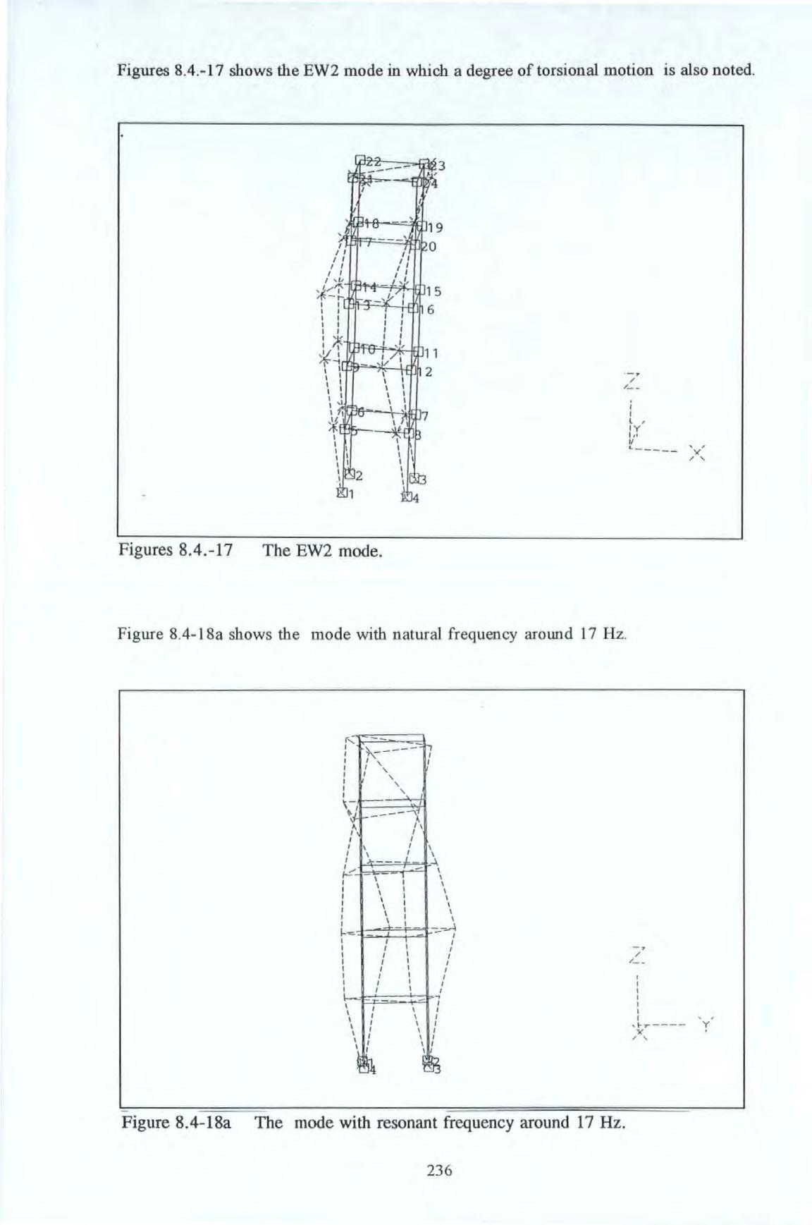
,.7__
Figures 8.4.-17 The EW2 mode.
r-..... -I I I I ' I I : ' I ' I ' I I \- -"1 1 1 \ I I I I \ I \ I \ 1 \ I A - I \ I I I I I I I 1 I I 1 I I I I I I I 1 I I I I I I I I l- -e. - I I I I I I I I 1 I I I I I I I 1 I I I I I I I 1 I I I I I I I I--I I I I I I I I I I I I I I I I I I I I I I I I
Figure 8.4-18a shows the mode with natural frequency around 17 Hz.
236 I I l IY l oo 11 __ , '1(, ' -, / ,.__ I I I I I I I ' , ... r----- y 'I( / ' ,
Figure 8.4-18a The mode with resonant frequency around 17 Hz.
Figure
shows another view of this mode. It appears, but with some reservation, that this may be the second torsional T2 mode
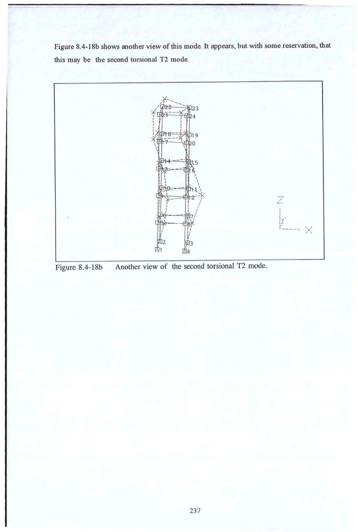 8.4-18b
2 37 -, / / __ I I l ' IY l o• 11 .. ____ _ )( / '
Figure 8.4-18b Another view of the second torsional T2 mode
However for the higher frequency modes , it becomes increasing difficult to classify them in the same as the lower frequency modes. For instance, the modes with frequencies around 18 and 24Hz are shown in Figures 8.4-18 and 8.4-19 respectively . As shown in these figures , motions in both the EW and NS directions are of comparable magnitudes and warping of the floor slabs are clearly visible.
Figures 8.4-18c The modes with frequencies around 18 Hz.
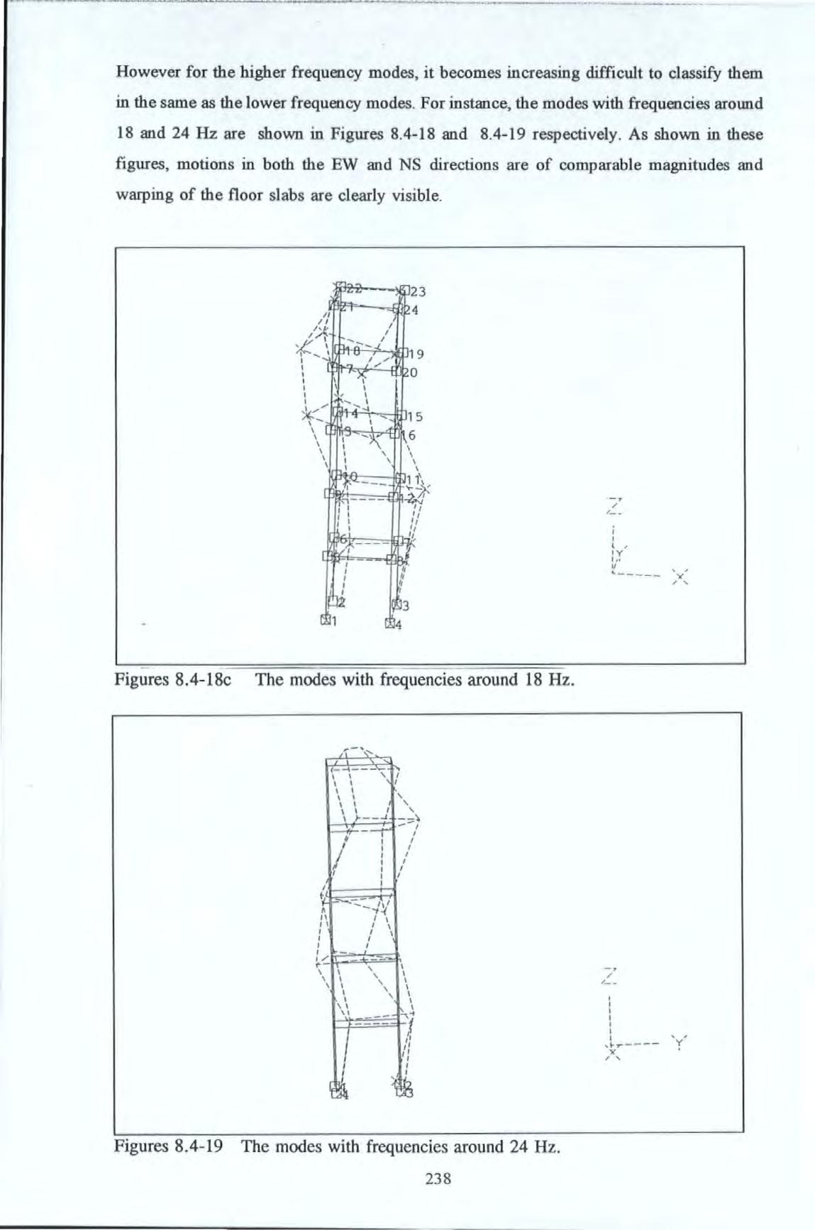
I -4, t; I I I I I I I ' I I I I ' 1 I I ' I f--..J -::=\ - I t I I I I I I I ! I I I I I I I I I Y11 I I 11 I I I I I I I I I1 / -:.. ,.- ' I \ I ' I \ I ' I \ I ' I I ' I I I \ I I \1 J, -I 11 11 11 I
238 I I l IIY · u __ -· / /_ I I I I I I I ,1(.,_r / ' ")( / ' ' , y
Figures 8.4- 19 The modes with frequencies around 24 Hz .
Similarly the results from the NS test series are given. Figure 8 .4-20 shows the swaying NS 1 mode. Again , the 4 grid lines along the Z direction are essentially straight lines. Some warping of the floor slabs occurred particularly at the top floor levels. 8.4-20

.. .. __...__._____ __ ___ _
r-• 11 11 I I I I I II I \-L I I a I Ill Ill lt11 11 \.. .. Ill" I t I I I I I • I \I I I I I I 11 11 11 , I I --11 " " t ---11 11 111 11 " 11 11 11 11 11 :I 1 I I I 11 (,
4 239, / / __ I I 'y' I ' , , '>( / '
The NS 1 mode
Figure 8.4-21 shows the torsional T1 mode. However this mode shape is less desirable than those obtained with the shaker acting in the EW direction The movements at the spatial points 4B 2 and 5A1 (points 19 and 21 in the figure) are unconformable to those shown in Figures 8.4-16 possibly owing to experimental errors

The torsional T 1 mode.
shows the NS2 mode
. I I I I I I' I Ill 11I 1/ ,'), ...' I 'I.I I I I I I ' I I .. I I I I I I I \---\ \ ' \ , '( <::.-.0,.. / I I II I ---l I I ' ---lI I I I I I I I I I I I --\I I I I I I I I'I , 'I I I I I I I I I I I I I I I I I I I I I ' I I I I I I I I I I I l/ c
Figure 8.4-2 1
Figure 8.4-22
r----1\ I I \\ I I .-} / -:'- / /.,'\ I I I I I I / 1 I I I 11.J--' I I I I I I I / !-- ..,/ --!-1--i l n 1 // I \ I I \I // ,- tt:.r--- · : \ I : : '\--'\.-\ \ '\\,, The NS2 mode . 240 j I I I I I 'y' I I I I I I I ' ',")( ' ' I .. ..:, / '
Figure 8.4-22
Figures 8.4-23 to 8.4-25 show the three other modes with natural frequencies around 16, 18 and 25 Hz respectively . For the same reasons already described, it is difficult to classify these modes .
Figures 8.4-23 The mode with frequencies around 16Hz
Figures
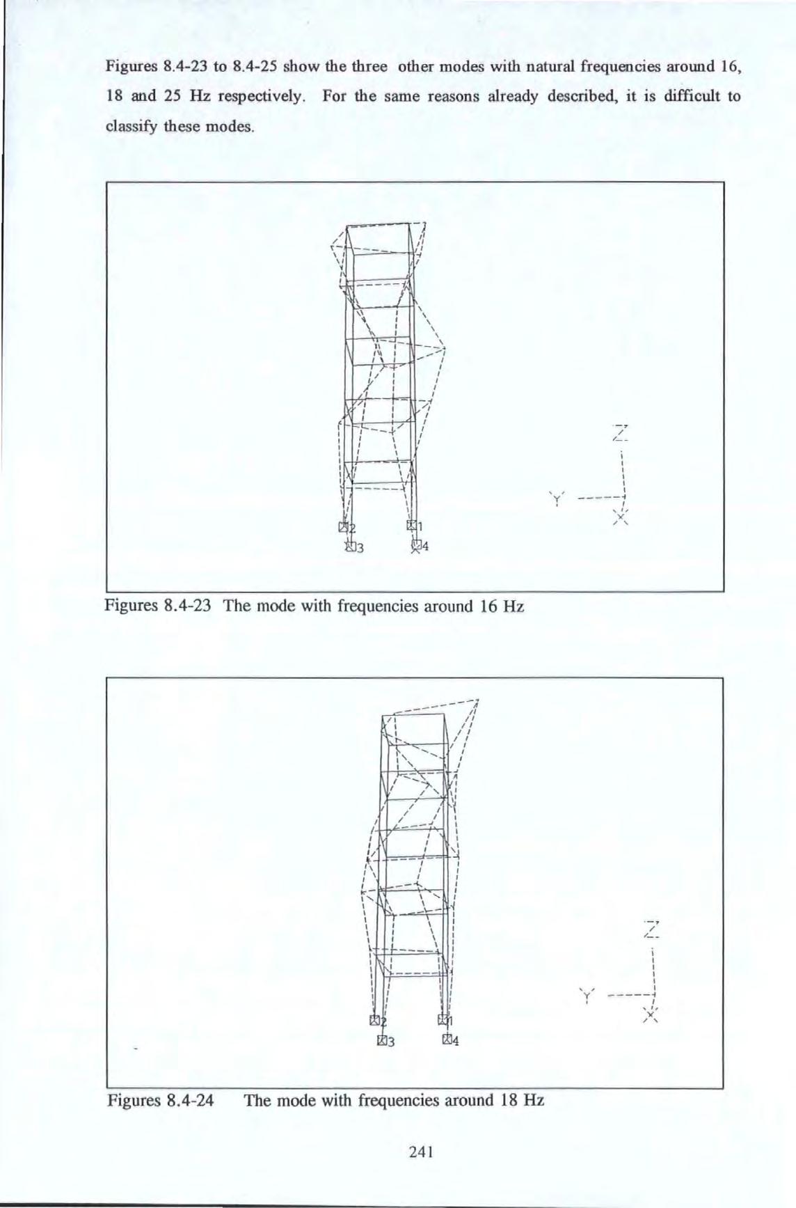
/ -II I -- 1 \ " I " I \ I I t\\ I I \ I 1/--i )' I /1 I V1 I I I I ( --.}/ I I I I I I I I I I I I I I I I I I I I 3 11 'I'-1 J, I ' ' ' ' \ ' t- --· --1- I I I I I I /-1 I I I I I I 1 4
8.4-24 I I I I / I I+ I \ \ I I.. 1'1 I I I I I l I I I I I I I I - -------:? / I I I to: ' I J', / I / I J I I I I I I '__ ..._ I ' I \ r I I I J_ I I I I '{ _I I I I I I I 11 I I / I I I I I I I I ;1 I I I I I ( I I I I :1 I I I I I I -1 I I I I I I I I I I I I I f The mode
frequencies
18 Hz 24 1 'y' 7,__ I I I I I I I I' ")( ' ' ' ' I I I I ' I y 0 I I' ")( ' '
with
around
A method, often used in civil engmeenng and practised by the BRE researchers, is to determine the deformed shape whilst a tested structure is still vibrating harmonically at one of the natural frequencies If modal density is light then the ratio of the relative kinematic responses (acceleration in this case or displacement if available) at any two spatial points will give a good estimate of the ratio of the mode shape coordinates. Note that this is only true if modes are well separated If an arbitrary spatial point is chosen as a fixed reference point then a plot of these ratios (called Motion Transmissibility or MT) on the spatial grid will give an estimate of the operating mode shape of that particular resonance mode
This technique was implemented slightly differently . The motion transmissibility FRF spectra were measured at all the measurement points whilst the structure was under pseudorandom instead of steady-state harmonic excitation. The MT at each resonance frequency was determined from the spectra provided by the spectrum analyzer from broad band random vibration. Providing modal density is slight, the method is feasible This technique is extremely useful because of the time savings over the steady state testing methods The MT of all the points (measured by a roving accelerometer called traveller) in the grid were referenced to the accelerometer fixed at the spatial point 5A I and orientated in a fixed direction . The three dimensional plots of the spatial deformation shapes at each of the

...,:..._. - _...> ......._';:--------- --] \\ \\ I \ I \ I \ I \ \ 'r I I ..'' \ \ /1 'I I I I I I I.I' I' I I I I I I I "' "'[ ,, /I l.l -- ' ' ' ' I I - / I I - / I I /.,. -I / 1>-_:;5._" I I I I I I I I I I I I I I I I I I I I I rlc I I II I ..:r-.. -T I I I I I I I I I ).( 1 4
I I I I I I ' y ' -- -- - 1 ' '')( / '
Figures 8.4-25 The mode with frequencies around 25 Hz
242
resonance frequencies were obtained with the use of the GINO graphic software. Like mode shapes, these plots provide an immensely useful tool to visualize the physics and behaviour of a structure at resonance or other conditions.
Figures 8.4-26a to 8.4-26d show the operating mode shapes at 2.36, l 0.2, 11.4 and 16.7 Hz with the exciter acting along the EW direction. There are some resemblances between these operating mode shapes and the corresponding mode shapes presented earlier. However for the two modes with very close natural frequencies, it should be borne in mind that the operating mode shapes will not approximate the true mode shapes.

243
f = 2.36Hz
f = 10.2Hz
f = ll.Hz
f = 16.7Hz

b a
d -
c
244
Figures 8.4-26a to 8.4-26d The operating mode shapes at 2 36, 10 2, 11.4 and 16 7 Hz with the exciter acting along the EW direction .
Figure 8.4-27a to 8.4-27e show the operating mode shape at 2 36, 5.3, 10 2, 11.4 and 16.7 Hz respectively with the exciter acting along the NS direction

= 11.4Hz
= 16.71iz
Figures 8 4- 27a to 8.4-27e The operating mode shapes at 2 36 , 5 3 , 10 2, 11.4 and 16 7 Hz with the exciter acting along the NS ctirection .
a b c f =
f =
f =
d e
f
2.36 Hz
5.31Hz
10.2Hz
f
24 5
The results show that most of the dominant modes of the tower occur below 25 Hz with the fwulamental modes occurring at about 2.3 Hz. The closeness of the EW I and NS 1 is believed to be due to the near symmetry in the structural, not architectural, details along the EW and NS directions. Because of the closeness of these modes, considerable coupling occurred and a mode could be excited even when the shaker was acting in a direction orthogonal to the mode. The torsional Tl mode occurred at a frequency roughly twice that of the fundamental swaying modes. The slightly lower frequency of the EW I mode than that of the NS I mode may suggest that the stiffness reduction due to the openings on one of the two infilled brick walls on the EW plane may be responsible, providing all the other structural factors concerning the walls stay the same in both the EW and NS planes.
All the mode shapes determined show considerable movements in the fifth floor. Hence, the placement of the exciter on this level was appropriate. The damping levels of all these modes are found to be around I% of critical damping. This is considered typical of most reinforced concrete structures and there is no cause for concern of any abnormality on this structure.
Tests results show that the natural frequencies of the Tl mode fluctuate with different force levels. However, due to the lack of sufficient data using SS excitation and insufficient frequency resolution, no conclusive statement can be made regarding the linearity or otherwise of this structure.

8.5 DISCUSSION
OF RESULTS
246
Because of the small size of the structure, very large amplitude motions of the structure have been excited. Considerable responses were measurable even at ground level which was five floor levels down from where the exciter was. Because SS tests can be carried out at variable steps, very fme frequency resolutions can be obtained at the expense of time. However, applying SS tests extensively will be too time-intensive and is not suitable to full scale field testing. The PRBS test method is extremely time efficient but cautions must be exercised especially regarding the problem of lack of frequency resolution in data. This is because the PRBS test method produces FRF spectra with a constant frequency resolution across the entire band of analysis. The results obtained in the field tests are largely consistent but are still inferior to those obtained from laboratory. Finally, it is shown that very useful structural information can be determined by performing full scale forced vibration testing on structures.

8.6 SUMMARY
247
Table 8.4-3. Modal parameters set determined from test data 220487001R (from 25 Hz PRBS tests with exciter acting EW and measurements made at grid point 5Ai in the EW direction).
where is the natural frequenc y of the rth mode is the modal damping factor of the rlh mode
Gr is the modal constant of the r 1 h mode
M' is the effective mass of the rlh mode r
C'r is the effective damping of the rlh mode
K' is the effective stiffness of the rth mode r
Table 8.4-4 . Modal parameters set determined from test data 230487009R (from 25 Hz PRBS tests with exciter acting NS and measurements made at grid point 5Al in the NS direction).

<..)r Gr M' r c· r I( MODE 1 2.357 0 0220 2.36e-5 4 .23e+04 2.77e+04 9 .29 e+6 MODE 2 5.615 0.0079 1.23 e-5 8.09e+04 4 .53e+04 l.Ole+8 MODE3 10.456 0 .0266 5.27 e-6 1.90e+05 6.64e+05 8 .19e+8 MODE4 6.160 0.0407 2.94 e-5 3.39e+04 1.07e+05 5 .08e+7 MODE 5 17 .535 0.0144 5.47 e-5 1.83e+05 5.79e+05 2.22e+9
<..)r G r M.' c · r K.' MODEl 2 .38 7 0 0210 2.05 e-5 4.87e+04 3 07e+04 1.10e+7 MODE2 5.760 0.0274 5.04 e-6 1.98e+ 05 3.93e+05 2.60e+8 MODE3 10.471 0 0461 3 12 e-6 3. 13e+05 1. 9 0e+ 06 1.35e+9 MODE4 12 183 0 0433 -3.16e-6 - 3.17e05 2. 10e+06 -1.8e+9 MODES 17.574 0.0176 1.7 6 e-6 5 .70e+05 2.2 le+06 6 .9 5e+9 24 8
Table 8.4-5 . Modal parameters set determined from test data 250487017 (from 25 Hz PRBS tests with exciter acting NS and measurements made at grid point 5B2 in the NS direction)
Table 8.4-6. Modal parameters set determined from test data 260487008R (from 25 Hz PRBS tests with exciter acting NS and measurements made at grid point 4A2 in the NS direction) .

I 250487017 w. G. M' c· I( I r r R MODEl 2.393 0 .0210 1.89 e-5 5.29e+04 3 34e+04 1.20e+7 MODE2 5 .6 13 -0 .049 1.04 e- 6 9.53e+05 -3 29e+06 1.19e+9 MODE3 I 0.248 -0.014 -4 .0 e-7 -2.20e+06 -4 0le+06 -9 .1 0e+9 MODE4 11.644 0.0255 2.21 e-6 4 5le+05 1.68e+06 2.4le+9 MODES 17.327 -0 .026 3 3 e-7 2.97e+06 -1.74e+07 3 .52e+10
1260;:700 w. G. M' r c · r I( I MODE 1 2.375 0.0213 1.84 e-5 5.44e+4 3.46e+4 1.21e+07 MODE2 5.568 0 0128 7.58 e-6 1 32e+5 1.18e+ 5 1.6le+08 MODE3 9.311 -0 . 110 9 . 12 e-6 1.1 Oe+5 - 1.42e+6 3 .75e+08 MODE4 11 .807 -0 .022 -2.4 e-6 -4.06e+5 - 1.38e+6 -2 .24e+09 MODES 16.948 0.0302 4 88 e-6 2.05e+05 1.32e+6 2.33e+09 249
Table 8.4-7. Modal parameters set determined from test data R25X021X (from 25 Hz PRBS tests with exciter acting EW and measurements made at grid p oint 5A2 in the EW direction) .
Table 8.4-8 . Modal parameters set determined from test data R25Y023Y (from 25 Hz PRBS tests with exciter acting NS and measurements made at grid point 5B2 in th e NS direction)

IR25X021X w, G, M; c · r K; I MODEl 2.357 0 0220 2.36E-5 4 23E4 9 290E6 2.766E4 MODE2 5 565 0 0128 9 64E-6 l.037E5 1.269E8 9.297E4 MODE3 10 359 0.0179 4 26E-6 2.347E5 9.946E8 5.497E5 MODE4 17 .549 0 .0 158 5.44E-6 l.836E5 2 233E9 l.329E6 MODE5 18 .859 0 .0019 3 .39E-7 2 .944E6 4 . 135EIO 1.046E6 MODE6 23 .555 0 .0526 l.48 E-5 6.722E4 1. 472E9 5.076E5
IR25Y0 23Y w, G, M,' c· r K' r I MODE 1 2.393 0.021 1.89E-5 5.288E4 1.1 95E7 3 .341E4 MODE2 5.451 0 015 -4 11 E-6 - 2.43 1E5 - 2 853E8 -2.546E5 MODE3 11.510 0 078 3 32E-6 3 010E5 1.5 74E9 3.439E6 MODE4 17 187 0 013 -9 52E-7 - 1.049E6 - 1. 223E l 0 -3 .124E6 MODE 5 23 .795 0 029 2 78E-6 3 .596E5 8 040E9 3.145E6 250
Table 8.4-9 . Modal parameters set determined from test data R25Y021X (from 25 Hz PRBS tests with exciter acting NS and measurements made at grid point 5A2 in the EW direction)
Tab l e 8.4-1 0. Modal parameters set determined from test data R25YO 17Y (from 25 Hz PRBS tests with exciter acting NS and measurements made at grid point 4A 1 in the NS direction) .

I R25Y021X (J), G, M ' r c· r K ' r I MODE 1 2.347 0 0167 -5 78E-6 -1.729E5 -3 .762E7 -8 .551E4 MODE2 5.512 0.012 -4 .02E-6 -2.486E5 -2 982E8 -2.098E5 MODE3 10 .337 0.016 -2.46E-6 -4 .054E5 -1.710E9 -8.588E5 MODE4 17.342 0 .021 -1. 71E-6 -5 . 832E5 -6 .925E9 -2 .752E6 MODE 5 24 320 0 016 -4 61E-6 -2 166E5 -5 058E9 -1.120E6
I R25Y017Y (J) , G, M,· c· r K, I MODE 1 2 385 0 018 1.69E-5 5.886E4 1 322E7 3 320E4 MODE2 5 545 0 008 3 26E-6 3 064£5 3 720E8 1.892E5 MODE3 10 633 0 .25 -4 .64E-6 -2 . 153£5 -9 .6 11E9 -7 373E5 MODE4 12 031 0 039 -4 98E-6 -2 004E5 -1.145E9 - 1.188E6 MODE 5 17 .292 0 033 2 80E-6 3 569E5 4.214E9 2 .623E6 MODE6 24 . 179 0.038 7.52E-6 1. 329£5 3 .068E9 1 55 1E6 25 1
Table 8.4-11. Modal parameters set determined from t es t data R25Y001Z (from 25 Hz PRBS tests with exciter acting NS and measurements made at grid point OAl in the Vertical direction)
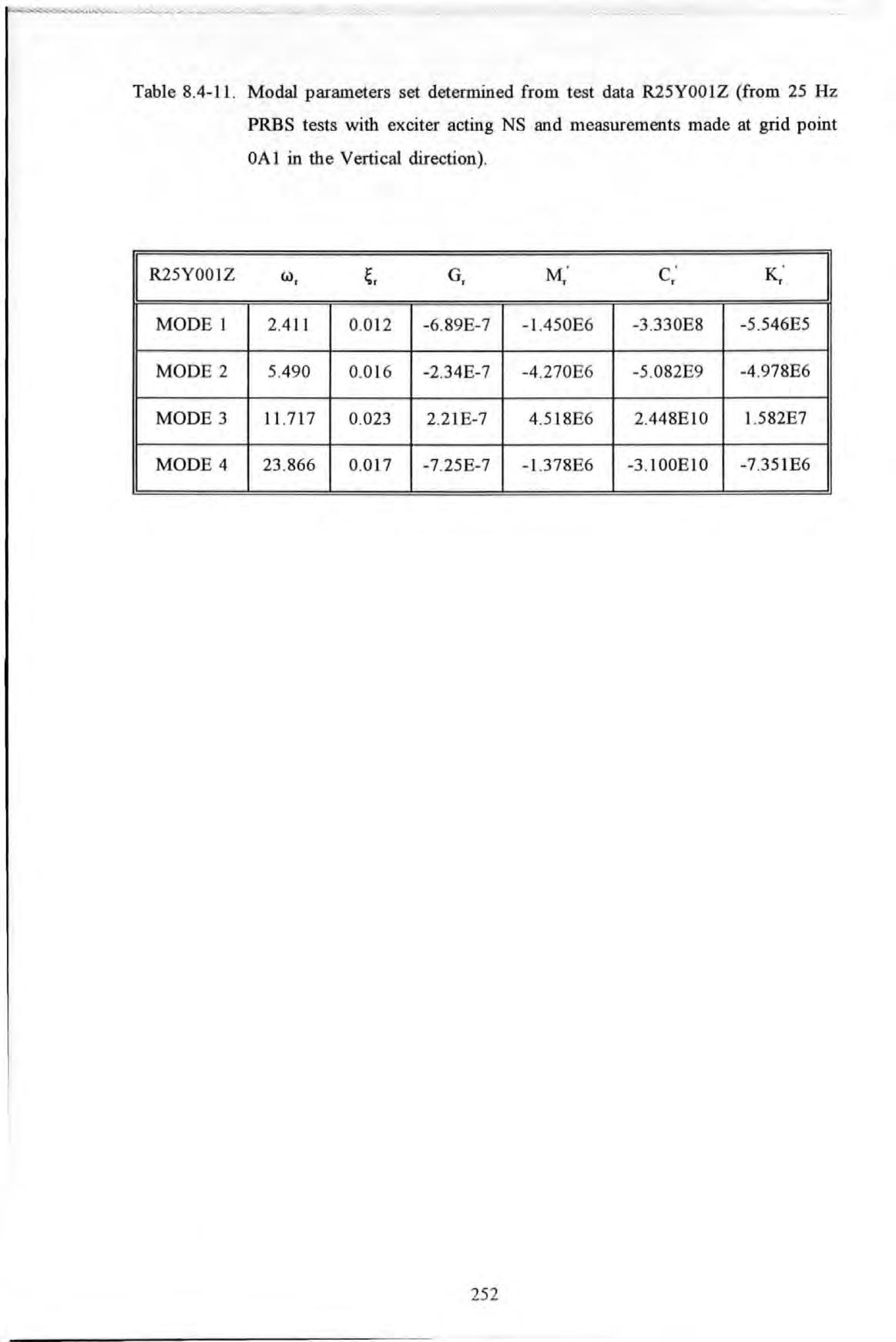
IR25Y001Z w, G, M' ' c · ' K; I MODE 1 2.4 11 0 012 -6.89E-7 -1 450E6 -3 330E8 -5 .546E5 MODE2 5.490 0.016 -2 34E-7 -4 270E6 -5.082E9 -4.978 E6 MODE3 11 717 0 023 2 2 I E-7 4 518E6 2 448El0 1 582E7 MODE4 23 866 0 017 - 7 25E-7 -1.378E6 -3 100El 0 -7 .351E6 252
CHAPTER9 CONCLUSIONS AND RECOMMENDATIONS
In addition to the discussions given and conclusions drawn for the individual chapters, this chapter provides an overall summary and a number of recommendations to bring this report to a close.
The application of experimental modelling to full scale civil engineering structures (using some of the techniques developed in the Experimental Modal Analysis field) has shown to be a worthwhile exercise and with good potentials. The testing techniques and the data analysis methods used are a significant departure from the established practices and techniques adopted in civil engineering as typified by the works of the EERL and the BRE. Therefore the objective of transferring this technology to civil engineering application has been fulfilled. Whilst it is recognized that civil engineering structures have many unique and different features which stand out from the rest of the engineering sphere, however further interest in the implementation of these technique to civil engineering should gather pace. The experimental approach advocated in this research should not be regarded as a substitute but a supplement to theoretical approach.
The literature reVIew reported in Chapter 2 shows that very few organisations or establishments are engaged in full scale forced vibration tests, especially in the UK. Reluctance and unenthusiastic reception the author has met in acquiring buildings for testing has reinforced this view that even professionals connected to civil engineering and the building industries do not realize the benefit of such research can bring. To increase their awareness must be a job of the highest priority.
253
The theory review reported in Chapter 3 shows that a great deal of the development in this technique origmates from other disciplines of engineering. Complexity of the theories, terminologies, jargons etc have placed many obstacles for civil/structural engineers to get a grip on this technology. Standardization of terminologies and practices should be an urgent development. The values of this emerging technology in relation to other established disciplines such as non-destructive testing, integrity testing etc have to be established.

The experimentation system used in this research has shown that moderate cost equipment can perform many functions that dedicated and sophisticated system can. Costs of instrumentation and microprocessor technologies continue to come down in recent years. Especially, the successes in miniaturization of microprocessors allow very sophisticated equipment once found only in a laboratory to be used in the field. Hence costs can no longer be obstacles to implementing this technology to full scale field testing.
The modal parameter extraction algorithm described in Chapter 5 is a simple yet practical tool to perform the requested task. The mechanics of the process of modal parameter extraction has been clearly explained and the success in constructing modal models of structures from experimental data illustrated. The simplicity of the algorithm is recognized as an ideal vehicle to teach new corners from civiUstructural engineering to acquaint with this technology.
The algorithm presented in Chapter 6 enables the spatial matrices of a structure to be determined directly from experimental data. Instead of very large matrices obtained from FE models, low order matrices are obtained from experimental models. These matrices provide information on a structure that can be easily understood by most civil/structural engineers and be used for validating analytical models, predicting the performance and evaluating the integrity of structures. The special tributes of this method are that the lack of frequency resolution of data measured near resonance is not critical (while this is the case with most modal methods) and that spatial measurements can be utilized in conjunction with local measurements for constructing models. Although this study has shown that so far this technique only works well for simple laboratory scale test piece, its successful application to large scale civil engineering structures can one day be realized providing that further efforts be directed to this technology in the experimentation and computing fronts .
254
APPENDIX 4.5.2
LISTING OF THE CONTROL PROGRAM
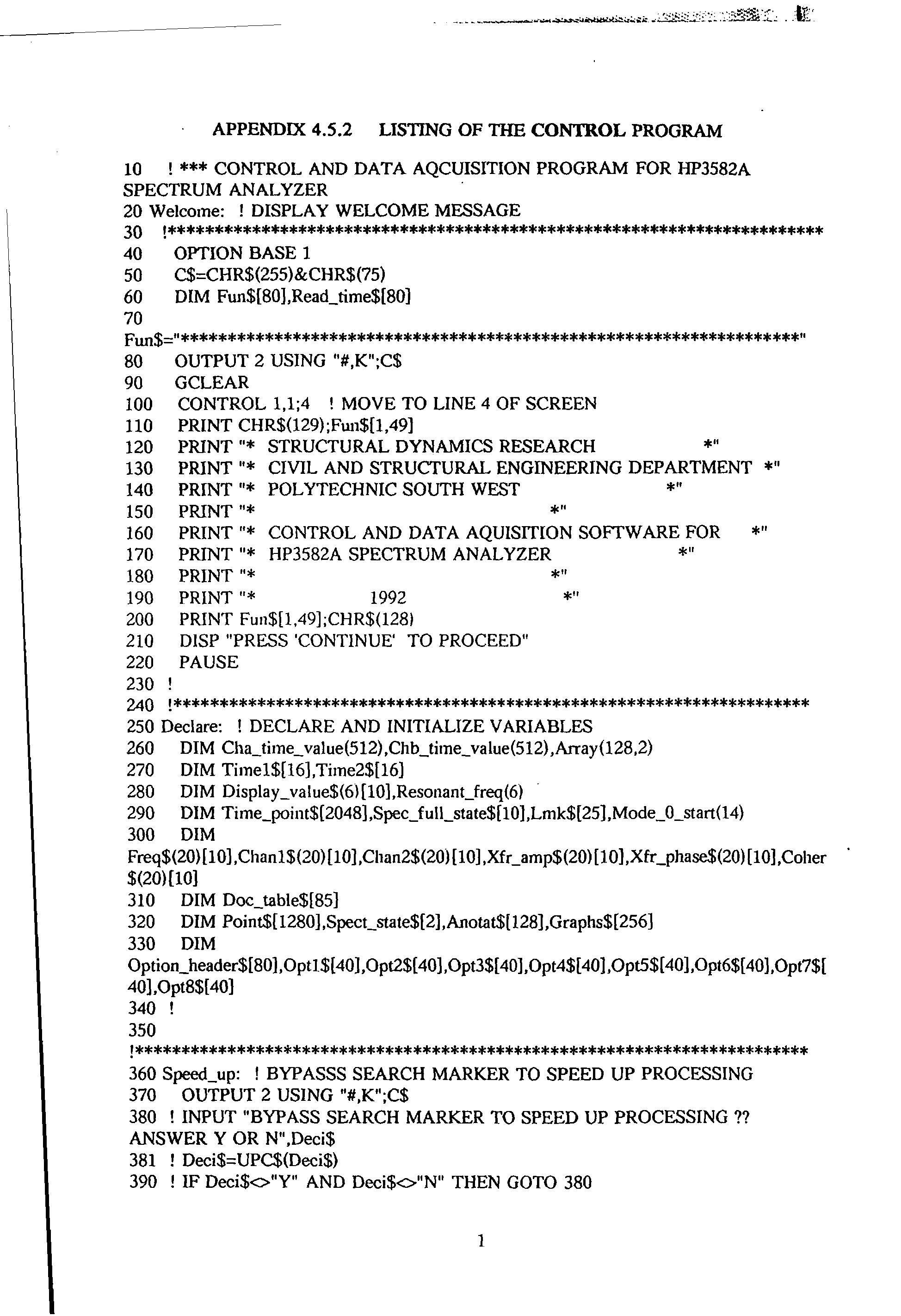
10 ! *** CONTROL AND DATA AQCUISITION PROGRAM FOR HP3582A SPECTRUM ANALYZER
20 Welcome: ! DISPLAY WELCOME MESSAGE
30 !***********************************************************************
40 OPTION BASE 1
50 C$=CHR$(255)&CHR$(75)
60 DIM Fun$[80],Read_time$[80]
70
Fun$="*******************************************************************"
80 OUTPUT 2 USING "#,K";C$
90 GCLEAR
100 CONTROL 1,1;4 ! MOVE TO LINE 4 OF SCREEN
110 PRINT CHR$(129);Fw1$[1,49]
120 PRINT "* STRUCTURAL DYNAMICS RESEARCH *"
130 PRINT"* CIVIL AND STRUCTURAL ENGINEERING DEPARTMENT *"
140 PRINT "* POLYTECHNIC SOUTH WEST *"
150 PRINT "* *"
160 PRINT"* CONTROL AND DATA AQUISITION SOFTWARE FOR *"
170 PRINT"* HP3582A SPECTRUM ANALYZER *"
180 PRINT "* *"
190 PRINT"* 1992 *"
200 PRINT Fun$[1,49];CHR$(128l
210 DISP "PRESS 'CONTINUE' TO PROCEED"
220 PAUSE
230 '
240 !*********************************************************************
250 Declare: ! DECLARE AND INITIALIZE VARIABLES
260 DIM Cha_time_value(512) ,Chb_time_value(512) ,Array(128,2)
270 DIM Timel$[16],Time2$[16]
280 DIM Display_value$(6)[10],Resonant_freq(6)
290 DIM Time_point$[2048],Spec_full_state$[10],Lmk$(25],Mode_O_start(l4}
300 DIM
Freq$(20)[10],Chanl$(20)[10],Chan2$(20)[10],Xfr_amp$(20)[10],Xfr_phase$(20)[10],Coher $(20}[10]
310 DIM Doc_table$[85]
320 DIM Point$[1280],Spect_state$[2],Anotat$[128],Graphs$[256]
330 DIM
Option_header$[80],0ptl$[40],0pt2$[40],0pt3$[40],0pt4$[40],0pt5$[40],0pt6$[40],0pt7$[ 40],0pt8$[40]
340 ! 350
!*************************************************************************
360 Speed_up: ! BYPASSS SEARCH MARKER TO SPEED UP PROCESSING
370 OUTPUT 2 USING "#,K";C$
380 ! INPUT "BYPASS SEARCH MARKER TO SPEED UP PROCESSING?? ANSWER Y OR N",Deci$
381 ! Deci$=UPC$(Deci$)
390 ! IF Deci$<>"Y" AND Deci$<>"N" THEN GOTO 380
]
430 ! IF Deci$="N" THEN
e.g 3rd OF MAY IS 0305",Current_date$ 580 Read_time$=" PRESS 'CONTINUE' AFTER READING MESSAGES
Master_menu 630 ON KEY 1 LABEL "RANDOM",3 GOSUB Periodic_random
640 ON KEY 2 LABEL "POINT_STORE" GOSUB Point_store
650 ON KEY 3 LABEL "GRAPHIC_STORE" GOSUB Graphic_store
660 ON KEY 4 LABEL "SPEC_PLOT" GOSUB Spec_plot
670 ON KEY 5 LABEL "NYQUIST_PLOT" GOSUB Nyquist_plot
680 ON KEY 6 LABEL "DOCUMENTATION" GOSUB Documentation
690 ON KEY 7 LABEL "SINE_SWEPT" GOSUB Sine_swept
700 ON KEY 8 LABEL "RELOAD_GRAPH" GOSUB Reload_graph
710 ON KEY 9 LABEL "RELOAD_TIME" GOSUB Reload_time
720 ON KEY 0 LABEL "SCANS" GOSUB Scans
730 ON KEY 11 LABEL "LOOK-ANY_FILE" GOSUB Look_any_file
740 ON KEY 12 LABEL "TIME_TRACE" GOSUB Time_trace
750 ON KEY 13 LABEL "UNDEFINED" GOSUB Undefined
760 ON KEY 14 LABEL "SPECT_SET_UP" GOSUB Spectrum_set_up
785 ! ***********SUB DEVICE TO ASSIGN 1/0 PATHS TO DEVICES
OUTPUT 2 USING "#,K";C$
PRINT" DEFAULT ADDRESS OF SPECTRUM ANALYZER IS 711 @SPECT"

PRINT" DEFAULT ADDRESS OF PHILIPS FUNCTION GENERATOR IS 704 @PHILIP"
PRINT" DEFAULT MASS STORAGE MEDIA IS THE RIGHT HAND DISC
440
" 590 600 !****************************************************************** 610 GOSUB
620
Bypass_marker$="N" 450 !ELSE 460 Bypass_marker$="Y" 470 ! END JF 480! 490 INPUT "ENTER CURRENT DATE
Device
GOSUB
770
781
782 !*********************************************************************** 783
**************** 790
800
801
802
803
804
806
807
808
809
810
811
2
Spin:GOTO Spin
!
Device: !
GCLEAR
ASSIGN @Spect TO 711
ASSIGN @Printer TO 701
ASSIGN @Philip TO 704 805 MASS STORAGE IS ":HP9122,700, 1"
PRINT
PRINT
PRINT
DRIVE (1)"
812 PRINT
813 PRINT" DEFAULT ADDRESS FOR PRINTER IS 701 @PRINTER"
814 PRINT
816 DISP CHR$(131);Read_time$;CHR$(128)
817 PAUSE
818 RETURN
831 !**********************************************
832 !******** SUB MASTER_MENU : TO DISPLAY KEY ASSIGNMENTS ******************
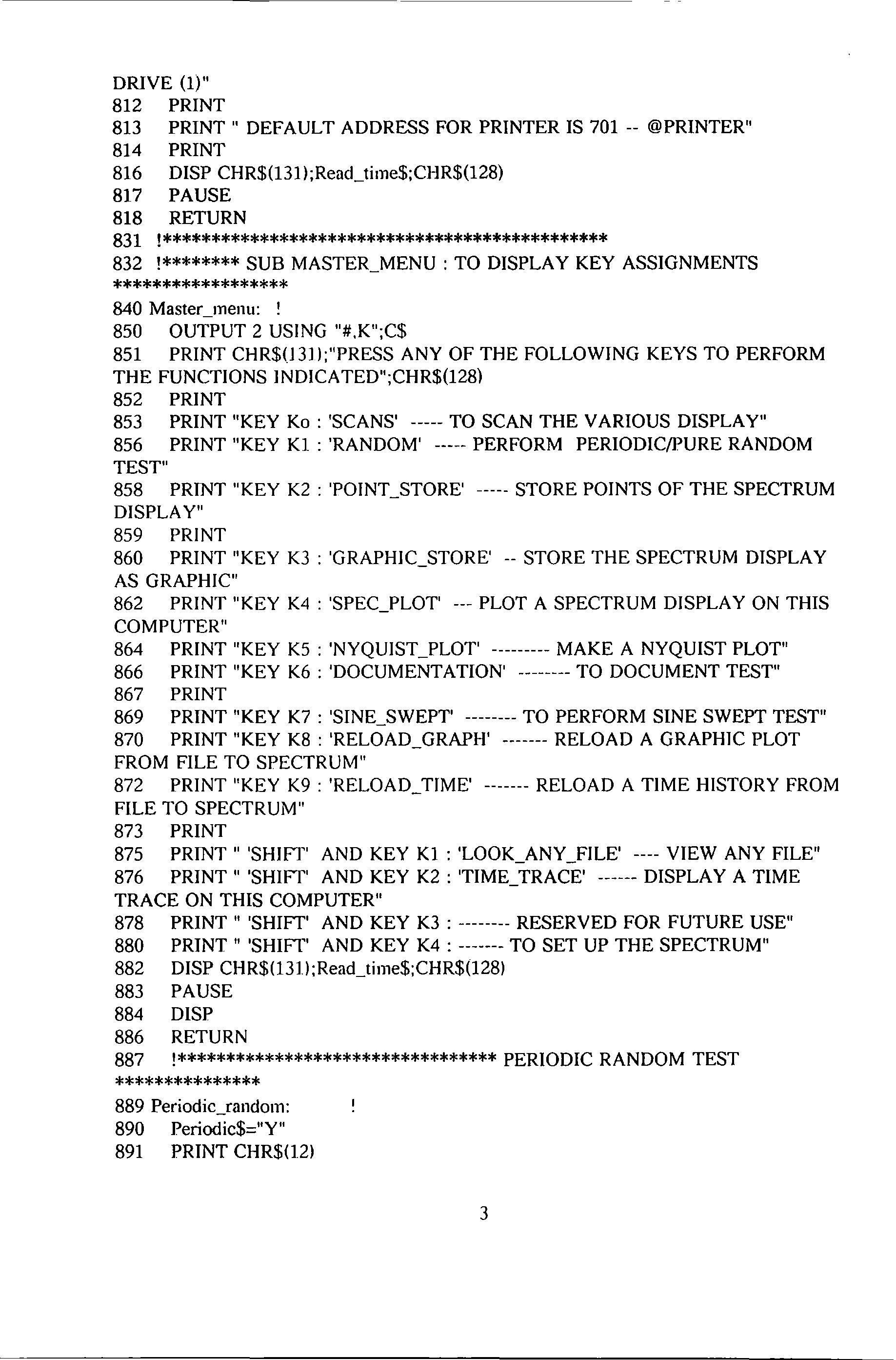
840 Master_menu: !
850 OUTPUT 2 USING "#,K";C$
851 PRINT CHR$03ll;"PRESS ANY OF THE FOLLOWING KEYS TO PERFORM THE FUNCTIONS INDICATED";CHR$(128)
852 PRINT
853 PRINT "KEY Ko : 'SCANS' TO SCAN THE VARIOUS DISPLAY"
856 PRINT "KEY K1 : 'RANDOM' PERFORM PERIODIC/PURE RANDOM TEST"
858 PRINT "KEY K2 : 'POINT_STORE' STORE POINTS OF THE SPECTRUM DISPLAY"
859 PRINT
860 PRINT "KEY K3 : 'GRAPHIC_STORE' STORE THE SPECTRUM DISPLAY AS GRAPHIC"
862 PRINT "KEY K4 : 'SPEC_PLOT' PLOT A SPECTRUM DISPLAY ON THIS COMPUTER"
864 PRINT "KEY K5 : 'NYQUIST_PLOT' MAKE A NYQUIST PLOT"
866 PRINT "KEY K6: 'DOCUMENTATION' --------TO DOCUMENT TEST"
867 PRINT
869 PRINT "KEY K7 : 'SINE_SWEPT' TO PERFORM SINE SWEPT TEST"
870 PRINT "KEY K8: 'RELOAD_GRAPH' -------RELOAD A GRAPHIC PLOT FROM FILE TO SPECTRUM"
872 PRINT "KEY K9: 'RELOAD_TlME' -------RELOAD A TIME HISTORY FROM FILE TO SPECTRUM"
873 PRINT
875 PRINT " 'SHIFT' AND KEY K1 : 'LOOK_ANY_FILE' VIEW ANY FILE"
876 PRINT" 'SHIFT' AND KEY K2 : 'TIME_TRACE' ------DISPLAY A TIME TRACE ON THIS COMPUTER"
878 PRINT " 'SHIFT' AND KEY K3 : RESERVED FOR FUTURE USE"
880 PRINT " 'SHIFT' AND KEY K4 : -------TO SET UP THE SPECTRUM"
882 DISP CHR$(13l);Read_time$;CHR$(128)
883 PAUSE
884 DISP
886 RETURN
887 !********************************* PERIODIC RANDOM TEST
***************
3
889 Periodic_random: 890 Periodic$="Y" 891 PRINT CHR$(12)
892 PRINT "ENTER TYPE OF RANDOM SIGNAL .... THERE IS NO DEFUALT" 893 PRINT 894 PRINT
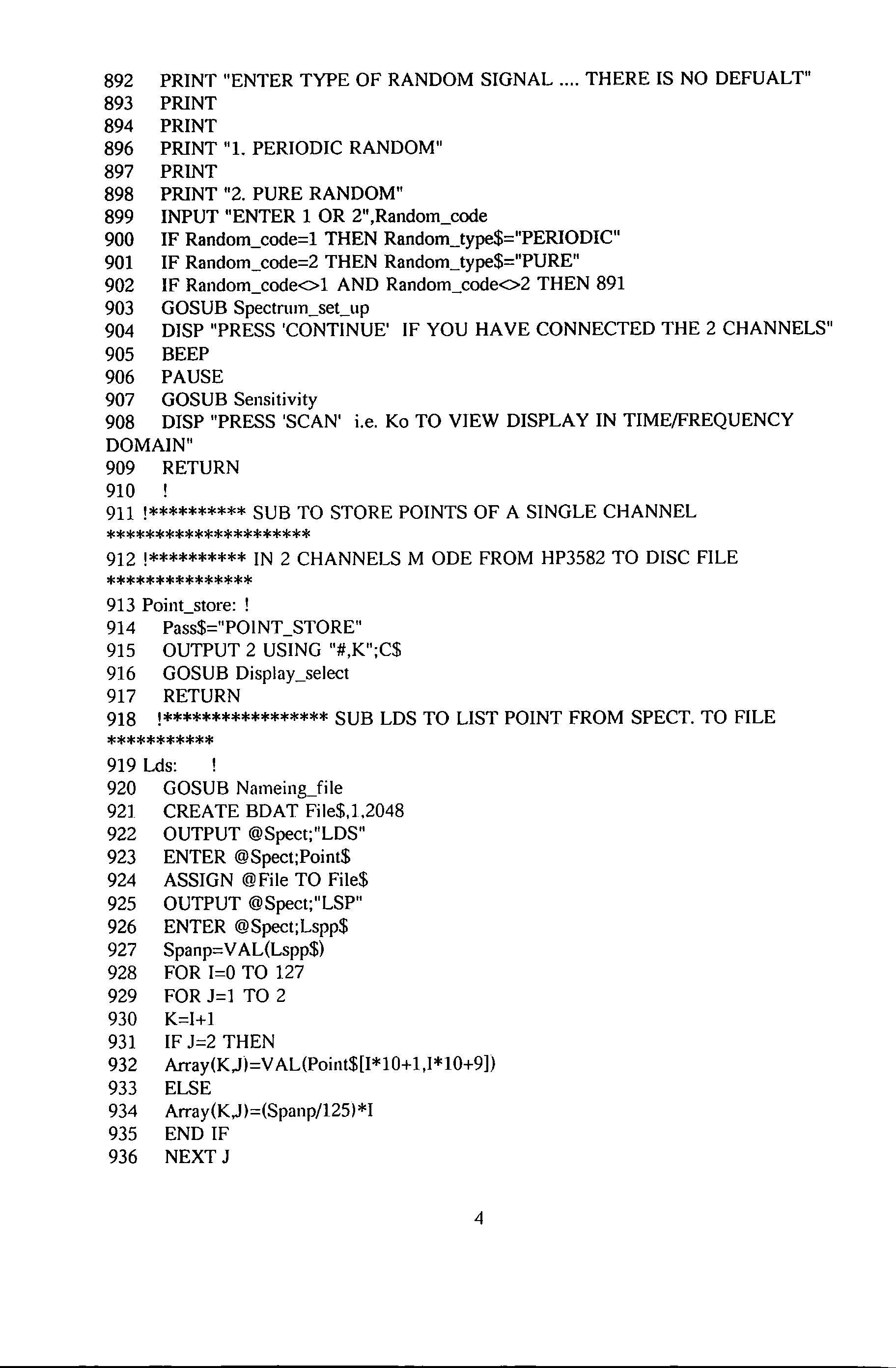
896 PRINT "1. PERIODIC RANDOM" 897 PRINT
898 PRINT "2. PURE RANDOM"
899 INPUT "ENTER 1 OR 2",Random_code 900 IF Random_code=1 THEN Random_type$="PERIODIC"
IF Random_code=2 THEN Random_type$="PURE"
IF Random_code<>1 AND Random_code<>2 THEN 891
GOSUB Spectnun_set_up 904 DISP "PRESS 'CONTINUE' IF YOU HAVE CONNECTED THE 2 CHANNELS"
GOSUB Sensitivity
DISP "PRESS 'SCAN' i.e. Ko TO VIEW DISPLAY IN TIME/FREQUENCY DOMAIN"
!********** SUB TO STORE POINTS OF A SINGLE CHANNEL
!********** IN 2 CHANNELS M ODE FROM HP3582 TO DISC FILE
LDS TO LIST POINT FROM SPECT. TO FILE
902
903
905
906
907
909
910
********************* 912
*************** 913
! 914
915
916 GOSUB
917 RETURN 918
*********** 919 Lds: ! 920 GOSUB Nameing_file 921 CREATE BOAT
922 OUTPUT @Spect;"LDS" 923 ENTER @Spect;Point$ 924 ASSIGN @File TO File$ 925 OUTPUT
926 ENTER @Spect;Lspp$ 927 Spanp=VAL(Lspp$) 928 FOR I=O TO 127 929 FOR J=l TO 2 930 K=l+l 931 IF J=2 THEN 932 Array(K,.H=V
933 ELSE 934 Array(K,J)=(Spanp/125)*I 935 END IF 936 NEXT J 4
901
BEEP
PAUSE
908
RETURN
911
Point_store:
Pass$=" POINT_STORE"
OUTPUT 2 USING "#,K";C$
Display_select
!*****************SUB
File$,1,2048
@Spect;"LSP"
AL(Point$[I*10+ 1,1*10+9])
TO STORE SPECTRUM PLOT AS GRAPHIC ********************
!PRINT "SET THE MOST FAVOURABLE AMPLITUDE REFERENCE ON SPECTRUM"
!PRINT "ALSO SELECT THE RIGHT DISPLAY"
'************** SUB GRAPH STORE TO STORE DISPLAY****************
!**************** AS GRAPHIC FILE ON DISC ****************************
ENTER @Spect USING "#,2A";Spect_state$
ENTER @Spect USING "#,256A";Graphs$
OUTPUT @Spect;"LAN"
ENTER @Spect;Anotat$
DISP "STORAGE OF DISPLAY AS GRAPHIC FILE HAS BEEN COMPLETED"
!*********** SUBROUTINE TO PLOT SPECTRUM DJSPLA Y ON COUMOPUTER *********
Spec_plot: !
PRINT "THIS IS SPEC_pLOT"
PRINT "THIS SUBROUTINE IS YET TO BE WRITTEN"
SUBROUTINE TO DJSPLA Y NYQUIST PLOT ON COMPUTER

937 938 939 940 941 ! 942 943 944! NEXT
OUTPUT
RETURN 945
946 Graphic_store: 947 OUTPUT
948 Pass$="GRAPH_STORE" 949 GOSUB
950
951
952
953
954
955 956
957
958 Graph_store: 959 GOSUB
960 CREATE
961 ASSIGN
962
963
964
965
966
967
968
969
970
971
972
973
974 975
976
977
978
979 RETURN 980 981 !***********
5
l ! PLOT Array(*)
@File;Array(*) ASSIGN @File TO* CALL Plot_data(File$) DISP "THE POINTS HAVE BEEN STORED"
!**************SUB
2 USING "#,K";C$
Display_select
! LOCAL @SPECT
!PRINT
RETURN
Nameing_file
BDAT File$,1,512
@File TO File$
OUTPUT @Spect;"HLTLFM,77455,1"
OUTPUT @Spect;"LFM,74600,128"
OUTPUT 1;Anotat$,Spect_stae$,Graphs$
OUTPUT @File;Graphs$,Spect_state$,Anotat$
ASSIGN @File TO*
OUTPUT @Spect;"RUN"
RETURN
************** 982 Nyquist_plot: 990 PRINT "THIS IS NYQUIST PLOT"
PRINT "THIS SUBROUTINE IS YET TO BE WRITTEN" 1000 RETURN 1061 ! 1062 !*********** SUB TO LOAD GRAPHIC FILE FROM DISC TO SPECTRUM BUFFER ******** 1070 Reload__graph: 1080 OUTPUT 2 USING "#,K";C$ 1081 GOSUB Nameing_file 1082 ASSIGN @File TO File$ 1083 ENTER @File;Graphs$,Spec_status$,Anotat$ 1084 OUTPUT @Spect USING "11N2A";"WTM,77455,1",Spec_status$ 1085 OUTPUT @Spect USING "16N256A";"HLTWTM,74600,128",Graphs$ 1086 OUTPUT @Spect;"WTAl,";Anotat$[1,32] 1087 OUTPUT @Spect;"WTA2,";Anotat$[33,64] 1088 OUTPUT @Spect;"WTA3,";Anotat$[65,96] 1089 OUTPUT @Spect;"WTA4,";Anotat$[97,128] 1090 ASSIGN @File TO * 1091 OUTPUT @Spect;"RUN" 1093 RETURN 1094 1095 !*******SUB TO LOAD TIME HISTORY FROM DISC TO SPECTRUM ***************** 1096 !******************* AND VICE VERSA ****************************** 1097 Reload_time: ! 1106 GOSUB Nameing_file 1107 GOSUB Initial_option 1108 Option_header$="TIME DOMAIN FACILITIES · " 1109 Optl$="STORE A TIME TRACE FROM HP3582 ONTO FILE" lllO Opt2$="RELOAD A TIME TRACE FROM FIE TO I-IP3582" 1111 GOSUB Option_menu 1112 IF Option<l OR Option>2 THEN 1114 GOSUB Warning 1120 GOTO 1111 1121 END IF 1122 ON Option GOSUB Time_store,Time_reload 1123 OUTPUT @Spect;"RUN" 1124 RETURN 1125 !***************SUB TO STORE TIME HISTORY FROM SPECT TO FILE ***** 1126 Time_store: 1127 CREATE BOAT File$,1,2300 1128 ASSIGN @File TO File$ 1129 OUTPUT @Spect;"HLTLFM,77454,5" 1130 ENTER @Spect USING "#,10A";Spec_full_state$ 1131 OUTPUT @Spect;"LFM,70000,1024" 6
991
1132 ENTER @Spect USING "#,2048A";Time_point$
1133 OUTPUT @File;Time_point$,Spec_full_state$
1134 ASSIGN @File TO*
1135 GOSUB Documentation ! WHY DOCUMENT AT THIS POINT?
1136 RETURN
1137 !**********SUB TO LOAD TIME HISTORY FROM FILE TO SPECT
******************
1138 Time_reload: !
1139 ASSIGN @File TO File$
1140 ENTER @File;Time_point$,Spec_full_state$
1141 OUTPUT @Spect USING "11NlOA";"WTM,77454,5";Spec_full_state$
1142 OUTPUT @Spect;"HLTWTM,70000,1024"
1143 OUTPUT @Spect USING "#,2048A";Time_point$
1144 ASSIGN @File TO *
1145 RETURN
1146
1147
!********** SUB WARNING TO MAKE SURE OPTION CHOSEN IS VALID*************
1148 Warning: !
1149 OUTPUT 2 USING "#,K";C$
1150 CONTROL 1,1;5
1152 PRINT
1153 PRINT " YOU HAVE SELECTED A WRONG OPTION"
1154 PRINT" YOU WILL BE GIVEN ANOTHER CHANCE"
1155 PRINT " OBSERVE THE CHOICES VERY WELL AND MAKE A VALID ONE"
1156 DISP CHR$(129);" PLEASE WAIT";CHR$(128)
1157 WAIT 10
1159 RETURN
1160
1161 !*********** SUB SCANS TO SCAN THE DISPLAYS *****************************
1162 Scans:
1163 OUTPUT 2 USING "#,K";C$
1164 Wait_time=20
1165 PRINT "THE DIFFERENT DISPLAYS FOR THE CURRENT INPUT "
1166 PRINT "MODE WILL NOW BE DISPLAYED BY THE SPECTRUM ANALYZER"
1167 PRINT
1168 PRINT "EACH DISPLAY WILL BE ON FOR ";Wait_time;" SECONDS "
1169 PRINT "AFTER WHICH TIME ANOTHER WILL REPLACE IT" 1170 PRINT
1171 OUTPUT @Spect;"TA1"
1172 DISP "CHAN. A TIME"
1174 WAIT Wait_time
1175 OUTPUT @Spect;"TAO"
1176 OUTPUT @Spect;"TBl"
1177 DISP "CHAN. B TIME"
1179 WAIT Wait_time
7
GOSUB Option_menu
1216 IF Option<l OR Option>3 THEN
GOSUB Waming 1218 GOTO 1215 1219 END IF 1220 OUTPUT 2 USING "#,K";C$
1221 PRINT" IF YOU WANT TO OBTAIN A HARD COPY"
1222 PRINT" ENTER Y ***ANY OTHER CHARACTER WILL"
1223 PRINT" BE IGNORED AND THE DATA WILL BE DISPALYED 11
1224 PRINT 11 ON THE SCREEN"
1225 INPUT "ENTER Y TO PRINT DATA 11 ,Yes$
1226 Yes$=UPC$(Yes$)
1227 IF Yes$="Y" THEN 1228 Printer_flag$="0N" 1229 END IF 1230 PRINT CHR$(12)
1231 ON Option GOSUB Read_s_file,Read_p_file,Look_file
1232 Printer_flag$="0FF" ! RESET PRINTER FLSG 1233 RETURN
1180 OUTPUT @Spect;"TBO" 1181 OUTPUT @Spect;"AA1" 1182 DISP "CHAN. A AMPLITUDE" 1184 CALL Amplitude_ref !WAIT Wait_time 1185 OUTPUT @Spect;"AAO" 1186 OUTPUT @Spect;"AB1" 1187 DISP "CHAN B. AMPLITUDE" 1189 CALL Amplit11de_ref !WAIT Wait_time 1190 OUTPUT @Spect;"ABO" 1191 OUTPUT @Spect;"AX1" 1192 DISP "XFR AMPLITUDE" 1194 CALL Amplitude_ref !WAIT Wait_time 1195 OUTPUT @Spect;"AXO" 1196 OUTPUT @Spect;"PX1" 1197 DISP "XFR PHASE" 1199 WAIT Wait_time 1200 OUTPUT @Spect;"PXO" 1201 OUTPUT @Spect;"CHl" 1202 DISP "COHERENCE" 1204 WAIT Wait_time 1205 OUTPUT @Spect;"CHO" 1206 DISP "FINISH" 1208 RETURN 1209 Look_any_file: 1210 GOSUB Initial_option 1211 Optl$="LOOK AT SINE FILE" 1212 Opt2$="LOOK AT PERIODIC FILE" 1213 Opt3$="DISPLA Y POINTS FILE" 1214 Option_header$=" 3 TYPES OF FILES CAN BE INSPECTED" 1215
1217
8
!*******************************
1235 !*********************** SUB READ_S_FILE **********************
1236 Read_s_file:
1237 GOSUB Nameing_file
1238 ASSIGN @File TO File$
1239 INPUT "INPUT NUMBER OF RECORDS TO READ",Record
1240 PRINT "SINE SWEPT DATA FILE IS ;";File$
1241 FOR I=1 TO Record
1242 ENTER @File;Freq$(1) ,Chan1$(1) ,Chan2$(1) ,Xfr_amp$(1) ,Xfr_phase$(I) ,Coher$(1)
1243 PRINT Freq$(1) ,Chan1$(1) ,Chan2$(1) ,Xfr_amp$(1) ,Xfr_phase$(!) ,Coher$(1)
1244 IF Printer_flag$="0N" THEN
1246 OUTPUT
@Printer;Freq$(1) .Chan1$(1) .Chan2$(1) ,Xfr_amp$(1) ,Xfr_phase$ (I) ,Coher$(I)
1247 END IF 1249 NEXT I
1250 ASSIGN @File TO*
1251 RETURN
1252 '***************** READ P FILE********************************
1253 Read_p_file:
1254 GOSUB Nameing_file
1255 ASSIGN @File TO File$
1256 INPUT "INPUT NO. OF RECORDS TO READ",Record
1257 PRINT "PERIODIC RANDOM TEST READING ARE FROM FILE ; ";File$

1258 FOR 1=1 TO Record
1259 ENTER
@File;Type_display$(1) ,Display_value$(1) ,Display_value$(2) ,Display_value$(3) ,Display_va lue$(4) ,Display_ value$(5) ,Display_value$(6)
1260 PRINT
Type_display$(1) ,Display_value$(1) ,Display_value$(2) ,Display_ value$(3) ,Display_value$(4)
.Display_value$(5) .Display_value$(6)
1261 IF Printer_flag$="0N" THEN
1263 OUTPUT
@Printer;Type_display$(1) ,Display_ value$(1) ,Display_ value$(21 ,Display_value$(3) ,Display _ value$(4) ,Display_value$(5) ,Display_value$(6)
SUB LOOK FILE TO DISPLAY POINTS FILE **********
1234
!****************
1270
1271
1272
1273
1274
1275 ASSIGN
1277
1278 END
9
1264 END IF 1266 NEXT I 1267 ASSIGN @File TO* 1268 RETURN 1269
Look_file:
GOSUB Nameing_file
ASSIGN @File TO File$
ENTER @File;Point$
PRINT Point$
@File TO* 1276 IF Printer_flag$="0N" THEN
OUTPUT @Printer;Point$
IF
1281
1282
!****************** SUB TIME TRACE * TO DISPLAY TIME TRACE
1283 Time_trace: ! ALL STATEMENTS ARE CURRENTLY BLANKED OUT
1284 OUTPUT 2 USING "#,K";C$
1285 INPUT "INPUT NAME OF FILE CONTAINING TIME TRACE",Time_file$
1286 ASSIGN @Time TO Time_file$
1287 ENTER @Time;Time_point$
1288 ! ASSIGN @Time TO *
1289 ! FOR I=l TO 1023 STEP 2
1290 ! Timel$=Dtb$(NUM(Time_point$[l*2-1,I*2-1])) ! Dtb$ SHOULD BE DTB$
1291 ! ! CAN'T CONTINUE UNTILL I KNOW THE MEANING OF THESE STATEMENTS
1292 ! ! DTB$, BTD
1293 RETURN
1294 Undefined:
1295 PRINT "THIS IS NOT YET DEFINED"
1296 RETURN
1297
1298 !*********** SUBROUTINE OPTION MENU ********************
1299 Option_menu: !
1300 OUTPUT 2 USING "#,K";C$
1301 GCLEAR
1302 Header_length=LEN (Option_header$)
1303 Center=(SO-Header_length)/2 ! SO THAT HEADER WILL BE PRINTED
1304 PRINT "SELECT YOUR OPTION"
1305 PRINT
1306 PRINT TAB(Center);Option_header$ ! AT ABOUT CENTRE OF LINE
1307 PRINT
1308 PRINT "1 FOR ";Opt1$
1309 PRINT "2 FOR ";Opt2$
1310 PRINT "3 FOR ";Opt3$
1311 PRINT "4 FOR ";Opt4$
1312 PRINT "5 FOR ";OptS$
1313 PRINT "6 FOR ";Opt6$
1314 PRINT "7 FOR ";Opt7$
1315 PRINT "8 FOR ";OptS$
1316 PRINT
1317 INPUT "WHICH OPTION?? ",Option
1318 IF Option<1 OR Option>8 THEN GOTO 1317
1319 CONTROL 1,1;14
1320 PRINT CHR$(131);"0PTION CHOSEN IS ";Option;CHR$(128)
1321 INPUT "ANSWER Y TO CONFIRM ; N TO CHANGE YOUR OPTION" ,Decision$
1322 Decision$=UPC$(Decision$)
1323 IF Decision$<>"Y" AND Decision$<>"N" THEN GOTO 1321
1324 IF Decision$="N" THEN GOTO 1317
1280 RETURN
********
10

IF Decision$="Y" THEN 1326 DISP "YOUR CHOICE HAS BEEN CONFIRMED" 1327 END IF 1328 RETURN 1329 ! 1330 !***********SUBROUTINE INITIAL_OPTION ************************* 1331 Initial_option: 1332 Optl$="" 1333 Opt2$="" 1334 Opt3$="" 1335 Opt4$='"' 1336 OptS$="" 1337 Opt6$="" 1338 Opt7$="" 1339 Opt8$="" 1340 Option_header$="" 1341 Option=O 1342 RETURN 1343 ! 1344 !**************** SUBROUTINE DISPLAY_SELECT****************** 1345 !******* ALLOWS YOU TO SELECT THE TYPE OF DISPLAY TO BE STORED******** 1346 Display_select: 1347 GOSUB Initial_option 1348 IF Pass$="GRAPH_STORE" THEN 1349 OUTPUT @Spect;"SC2" 1350 GOTO Jump! BYPASS OPTION 1351 END IF 1352 IF Pass$="POINT_STORE" THEN 1353 OUTPUT @Spect;"SC1" !USE LINEAR SCALE FOR POINT STORE 1354 GOTO Jump! BYPASS OPTION 1355 END IF 1356 GOSUB lnitial_option 1357 IF Pass$="SWEPT_SINE" THEN 1358 OUTPUT @Spect;"SC1" 1359 GOTO Sel_dis6 1360 END IF 1361 Option_header$="SCALE OF SPECTRUM PLOT: " 1362 Optl$="LINEAR SCALE" 1363 Opt2$="10 dB/VOLT SCALE" 1364 Opt3$="2 dB/VOLT SCALE" 1365 GOSUB Option_menu 1366 IF Option<l OR Option>3 THEN 1367 GOSUB Waming 1368 GOTO 1365 1369 END IF 1370 ON Option GOTO 1371,1373,1375 1371 OUTPUT @Spect;"SCl" 11
1325

1372 GOTO Jump 1373 OUTPUT @Spect;"SC2" 1374 GOTO Jump 1375 OUTPUT @Spect;"SC3" 1376 GOTO Jump 1377 Jump: ! 1378 GOSUB lnitial_option 1379 Option_header$="TYPES OF DISPLAYS TO BE STORED" 1380 Optl$="AMPLITUDE OF CHANNEL A" 1381 Opt2$="AMPLITUDE OF CHANNEL B" 1382 Opt3$="XFR AMPLITUDE" 1383 Opt4$="XFR PHASE" 1384 Opt5$="COHERENCE" 1385 Opt6$="ALL DISPLAYS" 1386 Opt7$="AL DISPLAYS EXCEPT AA" 1387 Opt8$="ALL DISPLAYS EXCEPT AA+ COHERENCE" 1388 GOSUB Option_menu
OUTPUT @Spect;"AAOABOAXOPXOCHOPAOPBO" 1391 ON Option GOTO Sel_dis1 ,Se!_d is2,Sel_d is3 ,Sel_dis4,Sel_dis5 ,Sel_dis6,Sel_dis7 ,Sel_d is8 1392 Display_retum: ! POINT OF RETURN FOR THE DISPLAY OPTIONS 1393 RETURN 1394 !********************************************************************* 1395 Sel_disl: 1396 Type_display=l 1397 OUTPUT @Spect;"AAl" 1398 DISP "CHANNEL A AMPLITUDE SPECTRUMJS TURNED ON" 1399 CALL Amplitude_ref 1400 IF Pass$="GRAPH_STORE" THEN GOSUB Graph_store 1401 IF Pass$="POINT_STORE" THEN 1402 GOSUB Lds 1403 ! GOSUB Select_marker 1404 END IF 1405 OUTPUT @Spect;"AAO" 1406 DISP "CHANNEL A AMPLITUDE SPECTRUMJS TURNED OFF" 1407 GOTO Display _return 1408 I 1409 Sel_dis2: 1410 Type_display=2 1411 OUTPUT @Spect;"AB1" 1412 DISP "CHANNEL B AMPLITUDE SPECTRUM IS TURNED ON" 1413 CALL Amplitude_ref 1414 IF Pass$="GRAPH_STORE" THEN GOSUB Graph_store 1415 IF Pass$="POINT_STORE" THEN 1416 GOSUB Lds 1417 ! GOSUB Select_marker 1418 END IF 12
1389
1419 OUTPUT @Spect;"ABO"
1420 DISP "CHANNEL B AMPLITUDE SPECTRUM IS TURNED OFF"
1421 GOTO Display_retum
1422 ! 1423 Sel_dis3: !
1424 Type_display=3
1425 OUTPUT @Spect;"AX1"
1426 DISP "AMPLITUDE OF RESPONSE FUNCTION ON"
1427 CALL Amplitude_ref 1428 IF Pass$="GRAPH_STORE" THEN GOSUB Graph_store
IF Pass$="POINT_STORE" THEN
@Spect;"AXO"
1434 DISP "AMPLITUDE OF RESPONSE FUNCTION TURNED OFF" 1435 GOTO Display_return
! 1437 Sel_dis4: 1438 Type_dis=4
1439 OUTPUT @Spect;"PX1"
1440 DISP "PHASE OF RESPONSE FUNCTION IS ON''
IF Pass$="GRAPH_STORE" THEN GOSUB Graph_store
IF Pass$="POINT_STORE" THEN
1447 DISP "PHASE OF RESPONSE FUNCTION IS OFF" 1448 GOTO Display_return 1449 ! 1450 Sel_dis5: 1451 Type_display=5
1452 OUTPUT @Spect;"CH1" 1453 DISP "COHERENCE FUNCTION NOW ON"
IF Pass$="GRAPH_STORE" THEN GOSUB Graph_store
IF Pass$=" POINT_STORE" THEN
@Spect;"CHO"
@Spect;"AA1"
1466 DISP "CHANNEL A AMPLITUDE IS ON"
1429
1430
GOSUB Lds 1431 GOSUB Select_marker 1432 END IF 1433 OUTPUT
1436
1442
1443
1444
1445
1441
GOSUB Lds
! GOSUB Select_marker
END IF 1446 OUTPUT @Spect;"PXO"
1454
1455
1456
1457
1458
GOSUB Lds
! GOSUB Select_marker
END IF 1459 OUTPUT
1460 DISP "COHERENCE FUNCTION IS OFF" 1461 GOTO Display_return 1462 ! 1463 Sel_dis6: 1464 Type_display=1 1465 OUTPUT
13
1467 IF Pass$="SWEPT_SINE" THEN GOTO 1478
THEN
IF Pass$="GRAPH_STORE" THEN
THEN
IF Marker_reading$[1,10]="+9.990E+99" THEN
Amp_ref=Amp_ref+ 1 1490 OUTPUT @Spect;"AM"& VAL$(Amp_ref)
Freq$(Iil=Y AL$(Freql 1495 OUTPUT @Spect;"AAO"
1496 DISP "AMPLITUDE OF CHANNEL A IS OFF" 1497 OUTPUT @Spect;"AB1"
1498 DISP "AMPLITUDE OF CHANNEL BISON"
1499 Type_display=2
1500 IF Pass$="SWEPT_SINE" THEN GOTO 1511
CALL Amplitude_ref
IF Pass$="POINT_STORE" THEN
! GOSUB Select_marker
IF Pass$="GRAPH_STORE" THEN
IF Pass$="SWEPT_SINE" THEN
ELSE
1517
"ERROR AT LINE 1470"
1470 GOSUB
1471
1472 GOTO
1473
1474
1475 GOSUB
1476 GOTO
1477 END IF 1478
1479 GOTO 1484 1480 ELSE 1481 DISP
1482 STOP 1483 END IF 1484 GOSUB
1485 Amp_ref=1 1486 OUTPUT
1487 GOSUB
1488
1489
1491
1492
1493
1494
1468 CALL Amplitude_ref 1469 IF Pass$="POINT_STORE"
Lds
! GOSUB Select_marker
1495
END IF
Graph_store
1495
IF Pass$="SWEPT_SINE"
"ERROR AT LINE 1437"
Search_marker
@Spec;"AM1"
Read_marker
GOTO 1487
END rF
Chan1$(Ii)=Marker_reading$
1501
1502
1503
1504
1505
1506
1507
1508
1511
1512
14
GOSUB Lds
GOTO 1528
END IF
GOSUB Graph_store 1509 GOTO 1528 1510 END IF
GOTO
1513
1514 DJSP
1518 Amp_ref=1
1519 OUTPUT @Spect;"AMl"
1520 GOSUB Read_marker
1521 IF Marker_reading$[1,10]="+9.990E+99" THEN 1522 Amp_ref=Amp_ref+1
1523
1528 OUTPUT @Spect;"ABO"
1529 DISP "CHANNEL 8 AMPLITUDE IS OFF"
1530 OUTPUT @Spect;"AX1"
1531 DISP "AMPLITUDE OF RESPONSE FUNCTION IS ON"
1532 Type_display=3
1533 IF Pass$="SWEPT_SINE" THEN GOTO 1544 1534 CALL Amplitude_ref
1560
1515 STOP 1516 END IF 1517 GOSUB Search_marker
OUTPUT @Spect;"AM"&VAL$(Amp_ref) 1524 GOTO 1520 1525 END IF 1526 Chan2$(Ii)=Marker_reading$ 1527 Freq$0i)=V AL$(Freq)
1535
1536 GOSUB
1537 GOSUB
1538 GOTO 1561 1539 END IF 1540
Pass$="GHRAPH_STORE"
1541 GOSUB Graph_store 1542 GOTO 1561 1543 END IF 1544 IF Pass$="SWEPT_SINE"
1545 GOTO 1550 1546 ELSE
DISP
1548 STOP 1549 END IF 1550 GOSUB
1551 Amp_ref=l 1552 OUTPUT
GOSUB
1554 IF Marker_reading$[1,10]="+9.990E+99"
1555 Amp_ref=Amp_ref+ 1
OUTPUT
GOTO 1553
END IF
Xfr_amp$(1i)=Marker_reading$
IF Pass$="POINT_STORE" THEN
Lds
Select_marker
IF
THEN
THEN
1547
"ERROR AT LINE 1567"
Search_marker
@Spect;"AM1" 1553
Read_marker
THEN
1556
@Spect;"AM"&VAL$(Amp_ref) 1557
1558
1559
Freq$(Ii)=V
OUTPUT
DISP
OFF" 15
AL$(Freq) 1561
@Spect;"AXO" 1562
"AMPLITUDE OF RESPONSE FUNCTION IS
1564
1563 OUTPUT @Spect;"PX1"
DISP "PHASE OF TRANSFER FUNCTION IS ON" 1565 Type_display=4 1566 IF Pass$="POINT STORE" THEN 1567 GOSUB Lds 1568 GOSUB Select_marker 1569 GOTO 1585 1570 END IF 1571 IF Pass$="GRAPH_STORE" THEN 1572 GOSUB Graph_store 1573 GOTO 1585 1574 END IF 1575 IF Pass$=" SWEPT_SINE" THEN 1576 GOTO 1581 1577 ELSE 1578 DISP "ERROR AT LINE 1877" 1579 STOP 1580 END IF 1581 GOSUB Search_marker 1582 GOSUB Read_marker 1583 Xfr_phase$(Ti)=Marker_reading$ 1584 Freq$(Ii)=V AL$(Freq) 1585 OUTPUT @Spect;"PXO" 1586 DISP "PHASE MOF RESPONSE FUNCTION IS OFF" 1587 OUTPUT @Spect;"CH1" 1588 DJSP "COHERENCE FUNCTION IS ON" 1589 Type_display=5 1590 IF Pass$="POfNT_STORE" THEN 1591 GOSUB Lds 1592 GOSUB Select_marker 1593 GOTO 1609 1594 END IF 1595 IF Pass$="GRAPH_STORE" THEN 1596 GOSUB Graph_store 1597 GOTO 1609 1598 END IF 1599 IF Pass$="SWEPT_SINE" THEN 1600 GOTO 1605 1601 ELSE 1602 DISP "ERROR AT LINE 2117" 1603 STOP 1604 END IF 1605 GOSUB Search_marker 1606 GOSUB Read_marker 1607 Coher$(Ii)=Marker_reading$ 1608 Freq$(Ii)=V AL$(Freq) 1609 OUTPUT @Spect;"CHO" 1610 DISP "COHERNCE FUNCTION IS OFF" 16
1613 Sel_dis7: 1614 OUTPUT @Spect;"AB1"
1615 DISP "CHANNEL B AMPLITUDE SPECTRUM IS ON"
1616
1617 CALL Amplitude_ref
1618 IF Pass$="GRAPH_STORE" THEN GOSUB Graph_store
1619 IF Pass$="POINT_STORE" THEN
1624 DISP "CHANNEL B AMPLITUDE SPECTRUM IS OFF"
1626 DISP "AMPLITUDE OF RESPONSE FUNCTION IS ON"
1628 CALL Amplitude_ref
1629 IF Pass$="GRAPH_STORE" THEN GOSUB Graph_store 1630 IF Pass$="POINT_STORE" THEN
1637
1638
1639 IF Pass$="GRAPH_STORE" THEN GOSUB Graph_store
1649
GOTO Display_retum
1611
1612
Type_display=2
1620 GOSUB
GOSUB
END IF
OUTPUT
Lds 1621
Select_marker 1622
1623
@Spect;"ABO"
1625 OUTPUT @Spect;"AX1"
1627 Type_display=3
1631 GOSUB
GOSUB
1633 END IF 1634 OUTPUT @Spect;"AXO"
Lds 1632
Select_marker
OUTPUT
1635 DISP "AMPLITUDE OF RESPONSE FUNCTION IS OFF" 1636
@Spect;"PX1"
DISP "PHASE OF RESPONSE FUNCTION IS ON"
Type_display=4
1641 GOSUB Lds 1642 GOSUB Select_marker 1643 END IF 1644 OUTPUT @Spect;"PXO" 1645 DISP "PHASE OF RESPONSE FUNCTION IS OFF" 1646 OUTPUT @Spect;"CH1"
DISP
ON"
Type_display=5
1640 IF Pass$="POINT_STORE" THEN
1647
"COHERENCE FUNCTION IS
1648
IF Pass$="GRAPH_STORE" THEN GOSUB Graph_store
GOSUB Lds
GOSUB Select_marker 1653 END IF 1654 OUTPUT @Spect;"CHO" 1655 DISP "COHERENCE FUNCTION IS OFF" 1656 GOTO Display_return 1657 1658 Sel_dis8: 17
1650 IF Pass$=" POINT_STORE" THEN 1651
1652
!
OUTPUT @Spect;"AB1"
DISP "AMPLITUDE SPECTRUM OF CHANNEL BISON"
Type_display=2
CALL Amplitude_ref
IF Pass$="GRAPH_STORE" THEN GOSUB
IF Pass$="POINT STORE" THEN
GOSUB Lds
GOSUB Select_marker
END IF OUTPUT @Spect;"ABO"
DISP "AMPLITUDE SPECTRUM OF CHANNEL B IS OFF"
OUTPUT @Spect;"AX1"
DISP "AMPLITUDE SPECTRUM OF RESPONSE FUNCTION IS ON"
Type_display=3
CALL Amplitude_ref
IF Pass$="GRAPH_STORE" THEN GOSUB Graph_store
IF Pass$="POINT_STORE" THEN
GOSUB Lds
GOSUB Select_marker
END IF OUTPUT @Spect;"AXO"
DISP "AMPLITUDE SPECTRUM OF RESPONSE FUNCTION IS OFF"
OUTPUT @Spect;"PX1"
DISP "PHASE SPECTRUM OF RESPONSE SPECTRUM IS ON"
Type_display=4
IF Pass$="GRAPH_STORE" THEN GOSUB Graph_store
IF Pass$="POINT_STORE" THEN
GOSUB Lds
GOSUB Select_marker
END IF OUTPUT @Spect;"PXO"
DISP "PHASE SPECTRUM OF RESPONSE FUNCTION IS OFF" GOTO
1659 1660 1661 1662 1663 1664 1665 1666 1667 1668 1669 1670 1671 1672 1673 1674 1675 1676 1677 1678 1679 1680 1681 1682 1683 1684 1685 1686 1687 1688 1689 1690 1691
1692
1693 ! *************SUB
******************************* 1694 Spectrum_set_up:
IF Periodic$="Y"
1696 IF Periodic$="Y"
DISP
1699 GOSUB Initial_option 1700 Opt1$="PERIODIC
SET UP" 1701 Opt2$="SWEPT SINE TEST" 1702 Opt3$="TRANSIENT DECAY TEST" 1703 GOSUB Option_menu 1704 IF Option<l OR Option>3 THEN 1705 GOSUB Warning 1706 GOTO 1703 1707 END IF 18
Display _return
SPECTRUM SET_UP
1695
THEN GOSUB Peri_ran_set_up
THEN 1709 1698
"SET UP OF HP3582A"
RANDOM
1708 ON Option GOSUB Peri_ran_set_up,Swept_sin_setup,Decay_set_up
1711 !************SUB PERl_RAN_SET_UP TO SET UP FOR************* 1712 !**********PERIODIC RANDOM TEST******************** 1713
IF Random_type$="PERIODIC" THEN
®Spect;"PS3" 1719 PRINT "UNIFORM PASS BAND WINDOW IS ON"
@Spect;"PS2" 1722 PRINT "HANNING PASS BAND WINDOW IS ON"
UP HP3582A FOR SWEPT SINE******************
@Spect;"PSl" 1730
"FLAT TOP PASS BAND WINDOW IS ON"
!***********SET UP HP3582A FOR DECAY TEST ***********************
! 1734
Common_set_up 1735 DISP "DIFFERENT TIME RECORD SHAPE CAN BE SET BY DIFFERENT FREQ SPAN OF ANALYSIS"
1736 WAIT 500 ! ISN'T THIS WAITING TOO MUCH?
1737 OUTPUT ®Spect;"RPO"
1738 DISP "REPIPITIVE HAS BEEN TURN OFF"
1739 OUTPUT @Spect;"FRO"
1740 DISP "FREE RUN HAS BEEN TURN OFF"
1741 OUTPUT @Spect;"PS3"
1742 DISP "UNIFORM PASS BAND WINDOW IS ON"
1743 GOSUB Sensitivity
1744 OUTPUT @Spect;"AR"
1745 DISP "ARM HAS BEEN TURN ON"
1746
GOSUB Sensitivity
1747 INPUT "IS THE CAPTURED TRACE O.K **ANSWER Y OR N **" ,Deci_cap$
1748 Deci_cap$=UPC$(Deci_cap$)
1749 IF Deci_cap$<>"Y" OR Deci_cap$<>"N" THEN GOTO 1747
1750 IF Deci_cap$="N" THEN GOTO 1746
1751 RETURN
1752
1753 !********** COMMON SET UP OF HP3582A FOR ALL TESTS ****************
RETURN
!
Peri_ran_set_up:
GOSUB
PRINT
1718 OUTPUT
1720 ELSE
OUTPUT
END
1724 PRINT 1725 RETURN
Swept_sin_setup:
GOSUB
OUTPUT
1731 RETURN
1709
1710
! 1714
Common_set_up 1715
1717
1721
1723
IF
1726 !**********SET
1727
1728
Common_set_up 1729
DISP
1732
1733 Decay_set_up:
GOSUB
19
1754 Common_set_up: 1755 OUTPUT 2 USING "#,K";C$ 1756 OUTPUT @Spect;"IM2"
1757 PRINT "BOTH CHANNELS ON" 1758 PRINT 1759 OUTPUT ®Spect;"AC2"
1760 PRINT "DC COUPLING FOR CHANNEL A FOR LOW SIGNALS" 1761 PRINT 1762 OUTPUT ®Spect;"BC2" 1763 PRINT "DC COUPLING FOR CHANNEL B FOR LOW SIGNALS"
@Spect;"RPI"
PRINT "REPETITIVE ON"
"FREE RUN ON"
PRINT 1771 OUTPUT @Spect;"AV2" 1772 PRINT "RMS AVERAGING ON FOR COHERENCE MEASUREMENT" 1773 PRINT 1774 OUTPUT ®Spect;"MD2" 1775 PRINT "ZERO START MODE"
PRINT 1777 ! IF Petiodic$="Y" THEN
! OUTPUT ®Spect;"SPSNU3" !SPS =25Hz SPAN. CHANGE THIS AS PER STRUCTURE
GOTO 1785 !QUICK BYPASS ! BUT IS THIS DESIRABLE?
INPUT "INPUT FREQUENCY SPAN MODE 1-14",Span$
WAIT 3
CALL Freq_span_mode(Span$)
Current_span$=Span$ ! VARIABLE USED IN SENSITIVITY
OUTPUT ®Spect;"SP"&Span$! SET UP FREQ. SPAN OF ANALYSIS
INPUT "ENTER NO. OF AVERAGES-- MODE NO. 1-4",No_average$
CALL Num_averages(No_average)
IF No_average>4 THEN
OUTPUT @Spect;"SH1" !SHIFT IS ON
"SHIFT IS ON"
AL$(No_average)
1766
1767
1770
1779
1780
1781
1786
1787
1788
1789
1790
1791
1792 No_average=No_average-4 1793 END
1794 No_average$=V
1795 OUTPUT
1796 OUTPUT
1797 RETURN 1798 1799 !*******************
1800
20
1764 OUTPUT
1765 PRINT
PRINT 1768 OUTPUT ®Spect;"FR1" 1769 PRINT
1776
1778
END IF
1782
1783
1784
1785
PRINT
WAIT 2
IF
@Spect;"NU"&No_average$
@Spect;"RE"
SUB SENSITIVITY ****************************
Sensitivity:
1801 OUTPUT 2 USING "#,K";C$
. 1802 PRINT "CONNECT THE TWO SIGNALS"
1803 PRINT
1804
OUTPUT @Spect;"SPS"! NEED TO CHANGE ANALYSIS SPAN
1805 ! ANALYSIS SPAN ALREADY SET IN COMMON_SET_UP
1806 ! SET A FAST SAMPLING RATE TO CHECK OVERLOAD
1807 1=10! THE HIGHEST SENSITIVITY TO LOW VOLT AGES
1808 Chan$="CHANNEL A"
1809 Status_bit=2
1810 Chan_set$="AS"! SET CHANNEL A SENSITIVITY
1811 OUTPUT @Spect;"RERP1FR1"! COMPLTETE A TIME RECORD SINCE OVERLOAD IS ONLY CHECKED AFTER A TIME RECORD IS FINISHED
1812 OUTPUT @Spect;Chan_set$& VAL$(1)
1813 !WAIT 50
1814 OUTPUT @Spect;"LSTO"! INTERROGATE OVERLOAD STATUS AND RESET BITS
1815 ENTER @Spect USING "#,B'';Overload
1816 Check_bit=BIT(Overload,Status_bit)
1817 DISP "CHECK BIT FOR ";Chan$;" IS ";Check_bit
1818 IF Check_bit=1 THEN GOTO 1820
1819 IF Check_bit<>1 THEN GOTO 1823
1820 OUTPUT @Spect;"RE"
1821 1=1-1
1822
GOTO 1811
1823 IF Chan$="CHANNEL B" THEN GOTO 1829
1824
Chan$="CHANNEL B"
1825 1=10
1826
1827
1828
Status_bit=3
Chan_set$="BS"
GOTO 1811
1829 OUTPUT @Spect;"LAS" 1830 ENTER @Spect;A_sensitivity$
1831 PRINT "CHANNEL A SENSITIVITY IS : ";A_sensitivity$
1832 OUTPUT @Spect;"LBS"
1833 ENTER @Spect;B_sensitivity$
1834 PRINT "CHANNEL B SENSITIVITY IS ; ";B_sensitivity$
1835 OUTPUT @Spect;"SP"&Current_span$ ! SET IN COMMON_SET_UP
1836 OUTPUT @Spect;"RE"
OUTPUT @Spect;"LSTO"!INTERROGAT OVERLOAD STATUS AND RESET
Status_bit=2
ENTER @Spect USING "#,B'';Overload
Check_bit=BIT(Overload,Status_bit)
1837 DISP "THE SPECTRUM IS NOW TAKING MEASUREMENTS! ... PLEASE WAIT" 1838 BITS 1839 1840 1841 1842 1843
1844
IF Check_bit=1 THEN DISP "OVERLOAD AGAIN ; RESTART RECORDING"
BEEP 1300,1
21
1845 WAIT 3 1846 END IF 1847 IF Check_bit=1 THEN GOTO 1801 1848 Status_bit=3 1849 Check_bit=BIT(Overload,Status_bit) 1850 IF Check_bit=1 THEN 1851 DISP "OVERLOAD AGAIN: RESTART RECORDING" 1852 BEEP 1300,1 1853 WAIT 3 1854 END IF 1855 IF Check_bit=1 THEN GOTO 1801 1856 Average_measur=Overload 1857 Check_bit=BIT(Average_measur,6) !CHECK IF AVERAGE IS COMPLETE 1858 IF Check_bit=1 THEN GOTO 1860 1859 IF Check_bit<>1 THEN GOTO 1838 1860 OUTPUT @Spect;"LSTO"!INTERROGATE OVERLOAD STATUS 1861 Status_bit=2 1862 ENTER @Spect
"#,B";Overloacl 1863 Check_bit=BIT(Overload.Status_bit) 1864 IF Check_bit=1 THEN 1865 DISP "OVERLOAD AGAIN; RESTART RECORDING" 1866 BEEP 1300,1 1867 WAIT 3 1868 END IF 1869 IF Check_bit=1 THEN GOTO 1801 1870 Status_bit=3 1871 Check_bit=BIT(Overload,Status_bit) 1872 IF Check_bit=l THEN 1873 DISP "OVERLOAD AGAIN; RESTART RECORDING" 1874 BEEP 1300,1 1875 WAIT 3 1876 END IF 1877 IF Check_bit=1 THEN GOTO 1801 1878 RETURN 1879 1880 !***************** SUB POSTER *************************** 1881 Poster: ! 1882 OUTPUT 2 USING "#,K";C$ 1883 GCLEAR 1884 GINIT 1885 GRAPHICS ON 1886 MOVE 1,80 1887 CSIZE 12,.5 1888 LABEL Poster$ 1889 RETURN 1890 '' 1891 !******************** SUB SINE SWEPT ; FOR SINE TESTING ********** 22
USING
1892 Sine_swept: ! 1893 OUTPUT 2 USING "#,K";C$ 1894 Poster$="SINE SWEEP TEST" 1895 GOSUB Poster 1896 Pass$="SWEPT SINE" 1897 INPUT "INPUT START FREQUENCY",Start_freq 1898 INPUT "INPUT FINISH FREQUENCY",Finish_freq 1899 INPUT "INPUT FREQUENCY STEP IN Hz ",Freq_step 1900 INPUT "INPUT TIME STEP IN SECONDS",Time_step 1901 Ac_input: 1902 INPUT "INPUT UPPER AC LEVEL IN FREE FORMAT",Upper_ac 1903 INPUT "INPUT LOWER AC LEVEL IN FREE FORMAT",Lower_ac 1904 INPUT "INPUT AC LEVEL TOTAL NUMBER OF STEPS",Ac_step 1905 GOSUB Freq_span_sel 1906 GOSUB lnitial_option 1907 Option_header$="SINE SWEPT TEST OPTIONS" 1908 Opt1$="SWEPT WITHOUT FlUNG" 1909 Opt2$="SWEPT WITH FlUNG" 1910 Swept_flag=O 1911 GOSUB Option_menu 1912 IF Option<O OR Option>2 THEN 1913 GOSUB Warning 1914 BEEP 1915 Swept_flag=l 1916 END IF 1917 IF Swept_flag=l THEN GOTO 1910 1918 FOR Ac=Lower_ac TO Upper_ac STEP (Upper_ac-Lower_ac)/Ac_step 1919 GOSUB Ac_dc_formating 1920
1921 Swept_with_file:
1922 File_or_not$="Y" 1923 Swept_no_filing: 1924 OUTPUT @Philip;"A";M$;"DOOW1";" " 1925 Ii=1 1926 FOR Freq=Statt_freq
Freq_step 1927 OUTPUT @Philip;"F";VAL$(Freq*.OOl);" " 1928 CONTROL 1,1;5 1929 PRINT
1930 PRINT 1931 PRINT
1932 OUTPUT ®Spect;"PS1IM2AC2BC2RP1FR1
1933 Current_span$="5"! MIGHT NEED TO CHANGE THE FREQ. SPAN 1934 GOSUB Sensitivity 1935 GOSUB Display_select 1936 Ii=Ji+1 1937 NEXT Freq 1938 IF File_or_not$<>"Y" THEN 1943 1939 Tot<ll_freq_step=li 23
ON Option GOTO Swept_no_filing,Swept_with_file
!
TO Finish_freq STEP
"DRIVING FREQUENCY NOW = ";Freq;" HZ"
"AC LEVEL NOW= ";Ac;" VOLTS P-P"
AV2MD2NU1"
1940 GOSUB File_sine_swept
1941 DISP "A FREQ_SWEPT CYCLE IS FINISHED, GOTO NEXT AC INCREAMENT; A NEW FILE NAME HAS TO BE GIVEN LATER NOT NOW"
1942 WAIT 4
1943 NEXT Ac
1944 Ii=1
1945 GOSUB Nameing_file
1946 RETURN
1947
1948
!************SUB AC-DC FORMATING ***********************
1949 Ac_dc_fonnating:
1950 IF Ac<=19.9 THEN Ac_ok
1951 PRINT "AC VALUE MUST BE LESS THAN 19.99 VOLTS, TRY AGAIN"
1952 GOTO Ac_input
1953 Ac_ok:
1954 As=Ac+100.0005
1955 Ac$=VAL$(Asl
1956 FOR 1=0 TO 2
1957 DlSP I
1958 IF Ac>=.2*10"1 THEN GOTO 1960
1959 M$=Ac$[4-I,7-I]
1960 NEXT I
1961 RETURN
1962
1963
!*************** SUB FILE_SlNE SWEPT**********************
1964 File_sine_swept:
1965 GOSU 8 Nameing_file
1966 CREATE BDAT File$,Total_freq_step,90

1967 ASSIGN @File TO File$
1968 FOR 1=1 TO Total_freq_step-1
1969 OUTPUT
@File; Freq$(1) ,Chan1$(1) ,Chan2$(l) ,Xfr_amp$(1) ,Xfr_phase$(1) ,Coher$(0
1970 CONTROL 1,1;12
1971 PRINT Freq$(1) ,Chan1$(I) ,Chan2$(I) ,Xfr_amp$(1) ,Xfr_phase$ (I) ,Coher$(1)
1972 NEXT I
1973 ASSIGN @File TO*
1974 RETURN
1975
1976
!************ SUB NAMEING_FILE **********************
1977 Nameing_file: 1978 1979
OUTPUT 2 USING "#,K";C$
PRINT "CURRENT DATE IS ";Current_date$
INPUT "ANSWER Y TO CONFIRM** N TO CHANGE DATE",Deci_date$
Deci_date$=UPC$(Deci_date$)
IF Deci date$<>"Y" AND Deci date$<>"N" THEN GOTO 1980 - -
IF Deci_date$="Y" THEN GOTO 1995
IF Deci_date$="N" THEN INPUT "INPUT NEW DATE",New_date$
1982
1984 1985
1980 1981
1983
24
1987 CONTROL 1,1;1 1988 PRINT "NEW DATE IS ";New date$ 1989 INPUT "IS THIS O.K? ;ANSWER Y *OR* N ",Deci_new$ 1990 Deci_new$=UPC$(Deci_new$) 1991 IF Deci_new$<>"Y" AND Deci_new$<>"N" THEN GOTO 1989
IF Deci_new$="N" THEN GOTO 1985
PRINT "CURRENT SERIAL NUMBER IS ";Current_ser$
INPUT "ANSWER Y TO CONFIRM *** N TO CHANGE***",Deci_ser_old$ 1998 Deci_ser_old$=UPC$(Deci_ser_old$) 1999 IF Deci_ser_old$<>"Y" AND Deci_ser_old$<>"N" THEN GOTO 1997 2000 IF Deci_ser_old$="Y" THEN GOTO 2012 2001 IF Deci_ser_old$="N" THEN
INPUT "INPUT NEW SERIAL NUMBER",New_ser$ 2003 PRINT 2004 CONTROL 1,1;1 2005 PRINT "NEW SERIAL NUMBER IS ";New_ser$&" " 2006 INPUT "IS THIS O.K? ;ANSWER Y *OR* N ",Deci_ser_new$
2007 Deci_ser_new$=UPC$(Deci_ser_new$)
2008 IF Deci_ser_new$<>"Y" AND Deci_ser_new$<>"N" THEN GOTO 2006
2009 IF Deci_ser_new$="N" THEN GOTO 2002
2010 Current_ser$=New_ser$
2011 END IF 2012 PRINT
2013 PRINT "CURRENT INDEX NUMBER IS ";Current_index$&" "
2014 INPUT "ANSWER Y TO CONFIRM*** N TO CHANGE***",Deci_ind_old$
2015 Deci_ind_old$=UPC$(Deci_ind_old$)
2016 IF Deci_ind_old$<>"Y" AND Deci_ind_old$<>"N" THEN GOTO 2014
2017 IF Deci_ind_old$="Y" THEN GOTO 2029
2018 IF Deci_ind_old$="N" THEN
2019 INPUT "INPUT NEW INDEX NUMBER",New_index$
2020 PRINT
2021 CONTROL 1,1;1
2022 PRINT "NEW INDEX NUMBER IS ";New_index$&" "
2023 INPUT "IS THIS O.K? ;ANSWER Y *OR* N ",Deci_ind_new$
2024 Deci_ind_new$=UPC$(Deci_ind_new$)
2025 IF Deci_ind_new$<>"Y" AND Deci_ind_new$<>"N" THEN GOTO 2023
2026 IF Deci ind new$="N" THEN GOTO 2019
2027 Cun·ent_index$=New_index$
2028 END IF 2029 PRINT
2030 File$=CurTent_date$&CmTent_ser$&Current_index$
2031 File$=File$[l,l0]
2032 DISP "FILE NAME IS ";File$;" ";CHR$(131);"WAIT";CHR$(128)
2033 WAIT 3
1986
1993
1994
1995 PRINT 1996
PRINT
1992
Current_date$=New_date$
END IF
1997
2002
25
2034 RETURN
2035
2036 !*********************SUB SEARCH_MARKER *********************
2037 Search_marker:
2038 OUTPUT @Spect;"LSP"
2039 ENTER @Spect;Freq_span$
2040 Freq_span=V AL(Freq_span$)
2041 Marker_position=(125/Freq_span)*(Freq-0)
2042 OUTPUT @Spect;"MN1MROMSOMBOMTOMP"& VAL$(Marker_position)
2043 RETURN
2044
2045 !**************** SUB READ MARKER *******************************
2046 Read_marker:
2047 OUTPUT @Spect;"LMK" 2048 ENTER @Spect;Lmk$
2049 Marker_freq$=Lmk$[12,20]
2050 Marker_reading$=Lmk$[1,10]
2051 DlSP "MARKER FREQ. & READING ARE :";Marker_freq$,Marker_reading$
2052 RETURN
2053
2054 !***************** SUB SELECT MARKER *************************
2055 Select_marker:
2056 OUTPUT 2 USING "#,K";C$

2057 PRINT "THE MARKER WILL BE READ AT THESE FREQUENCIES;"
2058 PRINT " 2.4. 5.6, 10.56. 12. 17.8, 25"
2059 Resonant_freq (1 l =2.4
2060 Resonant_freq(2)=5.6
2061 Resonant_freq(3)=10.56
2062 Resonant_freq(4)=12
2063 Resonant_freq (5)=17.8
2064 Resonant_freq(6)=25
2065 1=.1
2066 Freq=Resonant_freq (I)
2067 IF Bypass_marker$="Y" THEN
2068 Marker_position=025/25l*(Freq-O)
2069 GOTO 2076
2070 END IF
2071 GOSUB Search_marker
2072 GOSUB Read_marker
2073 GOTO 2077
2074 PRINT
2075 PRINT "THESE VALUES ARE FROM 'POINT$'
";Point$[Marker_position*10+ 1, (Marker_position+ 1)*10]
2076 Marker_reading$=Point$[Marker_position*10+ 1. (Marker_position+ 1 )*10]
2077 Option=Type_display
2078 ON Option GOTO 2079,2085,2091,2097,2103
2079 Chan1$(l)=Marker_reading$[1 ,10]
26
TO File$
2116 INPUT "DO YOU WANT A HARD COPY** Y OR N ** ",Dis_hard$

2117 Dis_hard$=UPC$(Dis_hard$)
2118 DISP "MARKER READINGS WILL BE STORED IN ";File$ 2119 OUTPUT @File_sel;Type_display$(Type_display) ,Display_value$( 1) .Display_value$(2) ,Display_value $(3),Display _ value$(4) ,Display_value$(5) ,Display_value(6)
2120 PRINT Type_display$(Type_display),Display_ value$(1) ,Display_value$(2) ,Display_value$(3),Displ ay_value$(4) ,Display_value$(5) ,Display_value(6)
2121 IF Dis_hard$="Y" THEN
2122 OUTPUT @Printer;Type_display$(Type_display) .Display_value$(]) ,Display_value$(2) ,Display_value$
2080 Display_value$(l)=Chan1$(l) 2081 Type_display$(Type_display)="CHANNEL# 1" 2082 IF 1>=6 THEN GOTO Escape 2083 1=1+1 2084 GOTO 2066 2085 Chan2$(1)=Marker_reading$[1,10] 2086 Display_ value$(1)=Chan2$(1) 2087 Type_display$(Type_display)="CHANNEL# 2" 2088 IF 1>=6 THEN GOTO Escape 2089 1=1+1 2090 GOTO 2066 2091 Xfr_amp$(I)=Marker_reading$[1,10] 2092 Display_value$(I)=Xfr_amp$(l) 2093 Type_display$(Type_display)="XFR_AMP " 2094 IF I>=6 THEN GOTO Escape 2095 I=I+1 2096 GOTO 2066 2097 Xfr_phase$(1 l=Marker_reading$[1,1 0] 2098 Display_value$(1)=Xfr_phase$(1) 2099 Type_display$(Type_display)="XFR_pHASE " 2100 IF 1>=6 THEN GOTO Escape 2101 l=I+1 2102 GOTO 2066 2103 Coher$(1)=Marker_reading$[1,10] 2104 Display_value$(l)=Coher$(1) 2105 Type_display$(Type_display)="COHERENCE " 2106 IF I>=6 THEN GOTO Escape 2107 1=1+1 2108 GOTO 2066 2109 Escape: IF Escape$="Y" THEN GOTO 2119 2110 INPUT "HOW MANY DISPLAY IN TOTAL?? ",Total_display 2111 DISP "ENTER NAME OF FILE FOR MARKER READINGS" 2112 WAIT 4 2113 GOSUB Nameing_file 2114 CREATE BOAT File$,Total_display,91 2115 ASSIGN @File_sel
27

(3) ,Display_value$(4) ,Display_value$(5) ,Display_value(61 2123 END IF 2124 INPUT "ANOTHER DISPLAY TO BE FOLLOWED ??",Deci_disp$ 2125 Deci_disp$=UPC$(Deci_disp$) 2126 IF Deci_disp$="Y" THEN 2127 Escape$="Y" 2128 GOTO 2132 2129 END IF 2130 ASSIGN @File_sel TO * 2131 Escape$="N" !RESET FLAG 2132 RETURN 2133 !******************************************************* 2134 !**********SUB FREQ_SPAN_SEL ********************************** 2135 Freq_span_sel: ! 2136 Mode 0 start(l)=l 2137 Mode_O_start(2)=2.5 2138 Mode 0 start(31=5 2139 Mode 0 start(4)=10 2140 Mode_O_start(5)=25 2141 Mode_O_start(61=50 2142 Mode_O_start(71=100 2143 Mode_O_start(81=250 2144 Mode 0 start(91=500 2145 Mode_O_start(10)=1000 2146 Mode_O_start(ll)=2500 2147 Mode 0 start(12)=5000 2148 Mode 0 stat1(131=10000 2149 Mode_O_stan(14)=25000 2150 FOR 1=1 TO 14 2151 IF Finish_freq-Mode_O_start(J)<O THEN 2152 Span_mode=l 2153 ELSE 2154 GOTO 2156 2155 END IF 2156 NEXT I 2157 OUTPUT @Spect;"MD2SP"& VAL$(Span_mode) 2158 RETURN 2159 2160 !****************SUB DOCUMENTATION OF TEST DATA ******************* 2161 Documentation: 2162 GOSUB lnitial_option 2163 Optl$=" CURRENT FILE NAME IS : "&File$ 2164 Opt2$=" CHANGE FILE NAME" 2165 Option_header$=" CHECK FILE NAME" 2166 GOSUB Option_menu 2167 IF Option>2 THEN 2168 GOSUB Warning 28
2169 GOTO 2166 2170 END IF 2171 ON Option GOTO Doc1_1,Doc1_2 2172 Doc1_1: 2173 GOTO Doc2 2174 Doc1_2: 2175 GOSUB Nameing_file 2176 Doc_table$[1,10]=File$ 2177 Doc2: ! 2178 GOSUB lnitial_option 2179 Option_header$="CHANNEL A IS:" 2180 Option_header$="CHANNEL A IS : " 2181 Opt1$=" #1650" 2182 Opt2$=" #1652" 2183 Opt3$=" #1653" 2184 Opt4$=" #1654" 2185 OptS$=" #1658 VERTICAL" 2186 Opt6$=" FORCE FROM DARTEC" 2187 Opt7$=" STRAINS" 2188 GOSUB Option_menu 2189 IF Option>7 THEN 2190 GOSUB Warning 2191 GOTO 2188 2192 END IF 2193 ON Option GOTO 2194,2196,2198,2200,2202,2204,2206 2194 Doc_table$[11,15]="#1650" 2195 GOTO 2208 2196 Doc_table$[11, 15]="#1652" 2197 GOTO 2208 2198 Doc_table$[11.15]="#1653" 2199 GOTO 2208 2200 Doc_table$[11,15]="#1654" 2201 GOTO 2208 2202 Doc_table$[11, 15]="#1658" 2203 GOTO 2208 2204 Doc_table$[11,15]="FORCE" 2205 GOTO 2208 2206 Doc_table$[11, 15]="STRAN" 2207 Option_header$="CHANNEL B IS : " 2208 Option_header$="CHANNEL B IS :" 2209 GOSUB Option_menu ! USE PREVIOUS SELECTIONS 2210 IF Option>7 THEN 2211 GOSUB Warning 2212 GOTO 2209 2213 END IF 2214 ON Option GOTO 2215,2217,2219,2221,2223,2225,2227 2215 Doc_table$[16,20]="#1650" 2216 GOTO 2228 29
2218
2220
2221
2222
2223
2225
2233
2234
2235
TYPE OF AMPLIFICATION"
Doe_table$[31,35]=" XlOO"
2248 GOTO 2251
2249 INPUT "ENETR APPLIED AMPLIFICATION IN 5-CHARACTERS",Amp$
2250 Doe_table$[31 ,35]=Amp$
2251 INPUT "ENTER MAX 5-CHARACTERS OF CODE OF LOCATION OF SIGNAL OF CHANNEL #A".A_Ioc_eode$ !Doc_tab\e$[41,45]
2252 PRINT Doe_table$
2253 Doe_table$[36,46]=A_loe_eode$
2254 GOSUB lnitial_option
2255 Option_header$="0RIENTATION OF SENSOR OF CHANNEL A"
2256 Opt1$=" XX"
2257 Opt2$=" YY"
2258 Opt3$=" VV"
2259 Opt4$=" **''
2260 GOSUB Option_menu
2261 IF Option>4 THEN
2262 GOSUB Warning
2263 GOTO 2260
Doe
2217
table$[16,20]="#1652"
GOTO
Doe_table$[16,20]="#1653"
2228 2219
GOTO
2228
Doe_table$[16,20]="#1654"
GOTO
2228
Doc_table$[16,20]="#1658"
GOTO
2224
2228
Doc_table$[16,20]="FORCE"
GOTO 2228
Doe_table$[16,20]="STRAN" 2228 OUTPUT @Speet;"LSP"
ENTER @Speet;Span$ 2230 Doc_table$[2l,30]=Span$
GOSUB Initial_option
Optl$="
2226
2227
2229
2231
2232
NO AMPLIFICATION"
Opt2$="
X10 AMPLIFICATION"
Opt3$="
X100 AMPLIFICATION"
Option_header$="
2237 GOSUB Option_menu 2238 IF Option>4 THEN 2239 GOSUB Warning 2240 GOTO 2237 2241 END IF 2242 ON Option GOTO
2243 Doe_table$[31,35]=" XO" 2244 GOTO 2251 2245 Doe table$[31.35]="
0" 2246 GOTO 2251
Opt4$=" OTHERS .. PLEASE ENTER" 2236
2243,2245,2247,2249
X1
2247
30
2264 END IF
2265 ON Option GOTO 2266,2268,2270,2272
2266 Doc_table$[47,50]="XX"
2267 GOTO 2273
2268 Doc_table$[47,50]="YY"
2269 GOTO 2273
2270 Doc_table$[47,50]="VV"
2271 GOTO 2273
2272
2273 INPUT "ENTER MAX 5-CHARACTERS OF CODE OF LOCATION OF SIGNAL OF CHANNEL #B",B toe code$ !Doc_table$[51,58]
2274 Doc_table$[51,58]=B_loc_code$
2275 Option_header$="0RIENTATION OF SENSOR OF CHANNEL B"
2289
2285 GOTO 2289
Doc_table$[47,50]="**"
2276 GOSUB Option_menu
GOSUB
GOTO
2281
2282
GOTO
2284
2277 IF Option>4 THEN 2278
Waming 2279
2276 2280 END IF
ON Option GOTO 2282,2284,2286,2288
Doc_table$[59,60]="XX" 2283
Doc_table$(59,60]="YY"
2286 Doc_table$(59,60]=="VV"
Doc_table$[59,60]=="**"
GOSUB Initial_option
Option_header$="TYPE
2291 Opt1$="XFR AMPLITUDE" 2292 Opt2$="XFR PHASE" 2293 Opt3$=="COHERENCE" 2294 Opt4$=="A - AMPLITUDE" 2295 Opt5$="B - AMPLITUDE" 2296 GOSUB Option_menu 2297 IF Option>5 THEN 2298 GOSUB Waming 2299 GOTO 2296 2300 END IF 2301 ON Option GOTO 2302,2304,2306,2308,2310 2302 Doc_table$[61,65]=" AMXFR" 2303 GOTO 2311 2304 Doc_table$(61,65]="PHXFR" 2305 GOTO 2311 2306 Doc_table$[61,65]="COHER" 2307 GOTO 2311 2308 Doc_table$[61,65]="AMP-A" 2309 GOTO 2311 2310 Doc_table$[61,65]=="AMP-B" 31
2287 GOTO 2289 2288
2289
2290
OF SPECTRAL PLOT"
2311 Doc_table$[66, 75] =A_sensitivity$
2312 Doc_table$[76,85]=B_sensitivity$
2313
2314
INPUT "ENTER 2-CHARACTER CODE FOR DOCUMENT FILE",Doc_char$
Doeu_file$="DOCUMENT"&Doc_ehar$[1,2]
2315 PRINT Doc_table$
2316 INPUT "IS THE DOCUMENT TABLE O.K.? ** Y OR N **",Deei doe$
2317 Deci_doc$=UPC$(Deei_doe$)
2318 IF Deei_doc$="N" THEN
2319 DISP "START DOCUMENT AGAIN"
2320 WAIT 3
2321 GOTO Documentation
2322 END IF
2323 INPUT "DO YOU WANT A HARD COPY?** Y OR N **",Deci_doc_hard$
2324 Deei_doe_hard$=UPC$(Deei_doc_hard$)
2325 IF Deei_doe_hard$="Y" THEN 2326 OUTPUT @Printer;CHR$(12) 2327 OUTPUT @Printer;Doe_table$
END IF
CREATE BOAT Docu_file$,1,90 2330 ASSIGN @Doe TO Doeu_file$
2339 ! ! SUBPROGRAM TO SELECT PROPER AMPLITUDE REFERENCE 2340 ASSIGN @Speet TO 711 2341 PRINT CHR$(12)
2342 PRINT " READ THIS MESSAGE CAREFULLY" 2343 PRINT
2344 PRINT " IF THE PRESENT AMPLITUDE REFERENCE IS O.K."
2345 PRINT " (i.e. THE DISPLAY ON THE SPECTRUM IS SATISFACTORY)" 2346 PRINT "THEN PRESS Y." 2347 PRINT
2348
PRINT "IF HOWEVER YOU WANT TO CHANGE THE AMPLITUDE"
2349 PRINT " REFERNCE, THEN PRESS N" 2350 INPUT "ANSWER Y OR N",Deei_amp$
2351 Deci_amp$=UPC$(Deei_amp$)
2352 IF Deei_amp$<>"Y" AND Deei_amp$<>"N" THEN 2350
2353 IF Deei_amp$="N" THEN
2354 OUTPUT 2 USING "#,K";CHR$(255)&"K"
2355 PRINT" INPUT AMPLITUDE REFERENCE LEVELS 1-9" 2356 PRINT " OR 0 IF O.K"
OUTPUT
ASSIGN
2333
2334 2335 '*************************** 2336 END 2337 !**********************************************************************
2328
2329
2331
@Doe;Doe_table$ 2332
@Doe TO*
RETURN
2338 SUB Amplitude_ref
32
2357 PRINT 2358 PRINT " FOR EACH LEVEL OBSERVE DISPLAY AND PRESS 0 WHEN SATISFIED"
2359 INPUT "INPUT LEVEL 1,2,3,4,5,6,7,8,9 ** OR ** 0 IF O.K",I
2360 IF I>9 THEN 2359
2361 IF 1=0 THEN 2367
2362 OUTPUT @Spect;"AM"&VAL$(1)
2363 CONTROL 1,1;16 2364 PRINT CHR$(131);"THE CURRENT LEVEL IS ";I;CHR$(128)
GOTO 2359
END IF 2367 PRINT CHR$(12)
SUBEND 2369 !*****************************************************
SUB Freq_span_mode(Span$)
GCLEAR 2396 PRINT CHR$(12) 2406 PRINT "SELECT FREQ. SPAN OF ANALYSIS (ZERO START MODE)"
2407 PRINT 2416 PRINT "------------------------
2426 PRINT " 1 1 Hz" 2436 PRINT " 2 ................. 2.5 Hz" 2446 PRINT " 3 5 Hz" 2456 PRINT " 4 ................. 10 Hz" 2466 PRINT " 5 ................. 25 Hz" 2476 PRINT " 6 ................. 50 Hz" 2486 PRINT" 7 100Hz" 2496 PRINT " 8 250 Hz" 2506 PRINT " 9 500 Hz" 2516 PRINT " 10 ................. 1 KHz" 2517 PRINT " 11 2.5 KHz" 2527 PRINT " 12 ................. 5 KHz" 2537 PRINT " 13 ................. 10 KHz" 2547 PRINT " 14................. 25 KHz" 2548 PRINT "--------------------------------------------------------" 2557 INPUT "SPAN MODE : l,2,3 14",Span 2567 IF Span<1 OR Span>l4 THEN 2386 2577 Span$=VAL$(Span) 2587 SUBEND 2597
2607 SUB Num_averages(No_average) 2617 GCLEAR 2627 PRINT CHR$(12) 2637 PRINT
AVERAGES" 2647 PRINT 2657 PRINT "----------------------------------------------------------" 2658 PRINT 2667 PRINT " 1 ..................... 4 AVERAGES" 33
2365
2366
2368
2376
2386
-------------------------------"
'***************************************************************
" ENTER NUMBER OF
PRINT "--------- --------------------------------------------------" 2737 INPUT "ENTER NO. OF AVERAGES : 1,2,3,4,5,6 OR 7" .No_average 2747 IF No_average<l OR No_average>7 THEN 2617 2748 PRINT CHR$(12)
2757 SUBEND
2758 !********************************************* PLOT SPECTRA
2760 SUB Plot_data(File$)
2770 Initialization: !
2780 C$=CHR$(255)&"K"
2790 OPTION BASE 1 ! CLEAR SCREEN
2800 INTEGER I,J,N,Num_zero_rows,Actual_rows,Ni
2810 DIM Title$[40],X$[30],Y$[30]
2840 GCLEAR
2850 OUTPUT 2 USING "#,K";C$
3000 MASS STORAGE IS ":HP9122,700,1"
3010 Sscale=l !DEFAAULT SCA;LING FACTOR
3400 Actual_rows=l28
3420 !*****************************************************************
3430 !
3440 Begin: ! REQUEST FILE NAME AND GRAPH LABELS

3580 Plot_type$=File$[5;1]
3590 Spect_type$=File$[6;1]
3600!
3610 IF Plot_type$="A" OR Plot_type$="B" OR Plot_type$="X" THEN ! ASK IF LINEAR OR DECIBEL SCALE IS TO BE USED.
3620 Linear_ask$="Y"
3630 PRINT CHR$(12)
3640 PRINT "DO YOU WANT LINEAR OR DECIBEL SCALE FOR SPECTRUM ??"
3650 PRINT " DEFAULT IS LINEAR SCALE"
3660 PRINT
3670 PRINT "PRESS 'ENTER' OR ENTER 'N' FOR DECIBEL SCALE"
3680 PRINT "ENTER 'Y' FOR LINEAR SCALE"
3690 INPUT "YOUR CHOICE OF SCALE DEFAULT IS LlNEAR",Linear_ask$
3700 Linear_ask$=UPC$(Linear_ask$)
3710 IF Linear_ask$<>"Y" AND Linear_ask$<>"N" THEN
3720 BEEP 3000,1
3730 GOTO 3630
3740 END IF
3750 END IF
3760 IF (Plot_type$="A" AND Spect_type$="X") OR Plot_type$="X" THEN
2677 PRINT
AVERAGES" 2687 PRINT " 3
AVERAGES" 2697 PRINT "
AVERAGES" 2707 PRINT"
AVERAGES" 2717 PRINT"
AVERAGES" 2727 PRINT
AVERAGES"
" 2 8
..................... 16
4 ..................... 32
5 ..................... 64
6 128
" 7 ..................... 256
2728 PRINT 2730
34
3770
Title$="AMPLITUDE TRANSFER FUNCTION"
. 3780 X$=" FREQUENCY (HZ)"
3790 Y$=" "
3800 IF Linear_ask$="N" THEN Y$="DECIBEL"
3810 GOTO 4140
3820 END IF
3830 IF (Piot_type$="P" AND Spect_type$="X") OR Plot_type$="P" THEN
3840
Title$="PHASE TRANSFER FUNCTION"
3850 Y$="DEGREES"
3860 X$="FREQUENCY (HZ)"
3870 GOTO 4140
3880 END IF
3890 IF (Piot_type$="C" AND Spect_type$="H") OR Plot_type$="C" THEN
3900 Title$="COHERENCE"
3910 X$="FREQUENCY (HZ)"
3920 Y$=" "
3921 OUTPUT 701 ;CHR$(12) !FORM FEED ON PRINTER TO NEW PAGE
3930 GOTO 4140
3940 END IF
3950 1F Plot_type$="A" OR Plot_type$="B" THEN
3960 IF Spect_type$="A" OR Spect_type$="L" OR Spect_type$="B" THEN
3970 Title$="AUTOSPECTRUM"
3980 X$="FREQUENCY (HZ)"
3990 Y$="VOLTS"
4000 IF Linear_ask$="N" THEN Y$="AMPLITUDE (DECIBEL)"
4001 IF Plot_type$="B" AND Spect_type$="L" THEN 4002 Y$="KN"
4003 END IF 4010 GOTO 4140
4020 END IF 4030 END IF 4040 IF Plot_type$="T" THEN 4050 Title$="TIME TRACE"
4060 Y$=" "
4070 X$="TIME (SEC.)"
4080 GOTO 4140
4090 END IF
4100 !
4110 INPUT "INPUT TITLE OF GRAPH ",Title$
4120 INPUT "INPUT TITLE FOR HORIZONTAL-AXIS'',X$
4130 INPUT "INPUT TITLE FOR VERTICAL AXIS",Y$
4140 OUTPUT 2 USING "#.K";C$
4150 PRINT "TITLE OF GRAPH IS '";Title$;""'
4160 PRINT
4170 PRINT "TITLE OF HORIZONTAL AXIS IS "';X$;""'
4180 PRINT
4190 PRINT "TITLE OF VERTICAL AXIS IS "';Y$;""'
4200 PRINT
35
4210 PRINT "ARE THESE O.K?"
4220 PRINT
4221 Fq_l$="Y"
4230 INPUT "ANSWER Y OR N DEFAULT IS Y",Fq_l$
4240 IF Fq_1$<>"Y" AND Fq_1$<>"N" THEN
4250 BEEP
4260 GOTO 4230
4270 END IF
4280 IF Fq_l$="N" THEN GOTO 4110
4290 PRINT "YOU'VE CONFIRMED THE LABELS"
4291 PRINT CHR$(12)
4292 CONTROL 1;12.12
4294 PRINT "DEFAULT SCALING FACTOR IS 1 : PRESS ENTER TO ACCEPT"
4296 INPUT "ENTER SCALING FACTOR",Sscale
4297 DISP "SCALING FACTOR IS : ";Sscale
4298 WAIT 1
4300 ! ***************************************************************
4310 Read_file: ! GET DATA FROM FILE
4320 IF Plot_type$="TT" THEN ! USE 'TT' TO BYPASS THIS. NEVER EXECUTED.
4330 ALLOCATE Time_array(Actual_rows,2) ,X(Actual_rows), Y (Actual_rows)
4340 ALLOCATE X_data_ window(Actual_rows), Y_data_ window(Actual_rows)
4350 ASSIGN @File TO File$ 4360 ON END @File GOTO 4380
4370
4380
4390 X(I)=Time_arny(I,l) 4400 Y(l)=Time_an·ay(l,2) 4410 NEXT I 4420 Max_x=MAX(X(*)) 4430 Min_x=MIN(X(*)) 4440 Min_y=MIN(Y(*)) 4450 Max_y=MAX(Y(*)) 4460 4470 MAT X_data_window= X 4480 MAT Y_data_window= Y 4490 GINIT 4500 GRAPHICS ON 4510 LDIR 0 4520 W=lOO*MAX(l,RATIO)! WIDTH 4530 H=100*MAX(l,l/RATIO) ! HEIGTH 4540 VIEWPORT .1*W,.98*W l5*H,.95*H 4550 WINDOW Min_x,Max_x,Min_y,Max_y 4560 FRAME 4570 GOTO 4820 4580 CLIP OFF 4590 Title$="TIME TRACE" 4600 X$="TIME (SEC.)" 36
ENTER @File;Time_an·ay(*)
FOR I=l TO Actual_rows
Y$=" "
! LABEL TITLE
5
6
Title_len=LEN (Title$)
Centre=(W- Title_len)/2
FOR P=.2 TO .2 STEP .025
FOR 1=1 TO Actual_rows
PLOT X(I),Y(J)
NEXT I
DEALLOCATE Time_an·ay(*l,X(*l,Y(*l
END IF
IF Manual_input$="SET" THEN 4910 INPUT "ENTER NUMBER OF PAIR POINTS TO BE PLOTTED i.e. NO. OF ROWS" ,Actual_rows 4920 GOTO 5280 4930 END IF 4940 OUTPUT 2 USING "#.K";C$
4950 DISP CHR$(130l;"READING FILE";CHR$(128);" ";CHR$(129);"PLEASE WAIT";CHR$(128!
4960 ASSIGN @File TO File$
ON END @File GOTO 5000 4980 ALLOCATE False_1 (128,2)

ENTER @File;False_1(*)
ASSIGN @File TO*
5260 Separate: ! SEPARATE DATA INTO Y_DATA AND X_DATA
5270 DISP CHR$(130);"PROCESSING ";CHR$(128);CHR$(129);"PLEASE WAIT";CHR$(128)
4610
4620
4630 CSIZE
4640 LORG
4650
4660
4670
4680
4690
4700
4710
4720 LORG
4730 CSIZE 3 4740 MOVE
4750 LABEL X$ 4760 ! LABEL
4770 LDIR 90 4780 LORG
4790 MOVE
4800 LABEL Y$ 4810 !LORG
4820
4830
4840
4860
4870
4880
4890
MOVE (Centre+P),(.99*H+P/2)
LABEL Title$
NEXT P
! LABEL X_AXIS
9
.8*W l*H
Y_AXIS
5
.015*W 5*H
8
!CSIZE 3
PRINT CHR$(12)
4850
GOTO 6750
4900
5250
4970
4990
5000 5001
********************************************************************
37
5280 ALLOCATE Y_data (Actual_rows) ,X_data (Actual_rows)
5290 IF Manual_input$="SET" THEN
5300 GOSUB Kbd_input
5310 GOTO Convert
5320 END IF
5340 ALLOCATE False_2(Actual_rows,2)
5350 MAT False_2= False_1
5360 DEALLOCATE False_1(*)
5380
5390 FOR I=1 TO Actual_rows
5400 FOR J=l TO 2
5410 IF J=2 THEN
5420 Y_data(l)=False_2(1,J)
5430 IF Plot_type$="A" THEN
5440 IF Linear_ask$="Y" THEN 5480
5450 IF Y_data(J)<=l.E-20 THEN Y_data(U=Last_y_data! SMOOTH SMALL
5460 Last_y _data=Y_data(I)
5470 Y_data(0=20*LGT(Y_data(I)) ! VALUES
5480 DUMMY LINE TO PREVENT INFINITE LOOP
5490 END IF
5500 ELSE
5510 X_data(J)=False_2(Ul
5520 END IF
5530 NEXT J
5531 Y_data(l)=Y _data(l)*Sscale
5540 NEXT I
5550 DEALLOCATE False_2(*l
5560 ASSIGN @File TO *
5570 !
5580 !**************************************************************
5590 Convert: !CONVERTING DATA TO FIT GRAPH WINDOW (DEFINED LATER)
5600 !OF (Q-100) * (20-70)
5610 ! NEGATIVE X VALUES NOT COVERED YET.
5620 ALLOCATE X_data_window(Actual_rows) ,Y _data_window(Actual_rows)
5630 ! OBTAIN MAX VALUES AND OTHER PARAMETERS TO CONTROL PLOTING AREA.
5640
5650 X_max=MAX(X_data(*))
5660 X_min=MIN(X_data(*))
5670 Y_max=MAX(Y_data(*))
5680 Y _min=MIN(Y _data(*))
5690 X_step=(X_max-X_min)/10
5700 Y_step=ABS( (Y _max- Y_min)/7)
5710 X_unit=X_min
5720 Y _unit= Y_m in
5730
5740 ! CONVERTING DATA
38
5750 FOR 1=1 TO Actual_rows
5760 X_data_window(l)=(X_data(I)/X_max)*100
5770 Y_data_window(l) =( (Y_data (I)- Y_min)/(Y_max- Y_min))*70+20
5780 IF Plot_type$="C" OR Plot_type$="P" THEN Y_data_window(I)=Y_data(I)
5790 ! IF Plot_type$="T" THEN Y_data_window(l)=Y_data(l)
5800 ! IF Plot_type$="T" THEN X_data_window(I)=X_data(l)
5810 NEXT I
5820! DEALLOCATE X_data(*),Y_data(*)! LEAVE FOR OBTAINING VALUES
5830
5840 !*********WRITE TITLE AND LABELS***********
5850 DISP
5860 OUTPUT 2 USING "#,K";C$
5870 GCLEAR
5880 GINIT
5890 GRAPHICS ON
5900 DEG
5910 W=100*MAX(l.RATIOI ! WIDTH
5920 H=lOO*MAX(l,l/RATIO) ! HEIGTH
5930 ! LABEL TITLE
5940 CSIZE 5
5950 LORG 6
5960 Title_len=LEN (Title$)
5970 Centre=(W-Title_len)/2
5980 FOR P=.2 TO .2 STEP .025
5990 MOVE (Centre+P),(.99*H+P/2)
6000 LABEL Title$ 6010 NEXT P
9
! LABEL X_AXIS
MOVE .8*W ,.13*H
Y_AXIS
..S*H
6110 LABEL Y$
6120 ' *********** BYPASS FOR PHASE AND COHERENCE PLOT
6130 IF Plot_type$="P" THEN
6140 CALL Phase(W,H,X_unit,X_step)
6150 GOTO Plot_points
6160 END IF
6170 IF Plot_type$="C" THEN
6180 CALL Coherence(W,H.X_unit,X_step)
6190 GOTO Plot_points
6200 END IF
6020
6050
6060
6030 LORG
6040 CSIZE 4
LABEL X$ 6070 ! LABEL
6080 LDIR 90 6090 LORG 5 6100 MOVE .015*W
**********
39
6210
6220 ! IF Plot_type$="T" THEN
6230 ! CALL Time(W ,H ,X_wtit,X_max, Y_writ, Y_max)
6240 ! FOR I=1 TO 256
6250 ! PRINT USING "3D.lOD,5X,3D.10D";X_data_window(I),Y_data_window(I)
6260 ! NEXT I
6270 ! GOTO Plot_points
6280 ! END IF
6290 !****.********************************************
6300 LDIR 0
6310 VIEWPORT .10*W,.98*W,.15*H,.95*H
6320 FRAME
6330 WINDOW 0,100,15,95
6340 AXES 5,5,0,15
6350 CLIP OFF ! TO ALLOW WRITING DIM OF AXIS
6360 ! PAUSE
6370
6380 ! ******************* DIMENSION X-AXIS***************
6390 LORG 6
6400 CSIZE 4
6410 FOR 1=0 TO lOO STEP 10
6420 MOVE 1,14.99
6430 LABEL USING "#,K";X_unit
6440 X_unit=X_unit+X_step
6450 NEXT I
6460
6470 ! ****************** DIMENSION Y-AXIS ****************
6480 LORG 8
6490 MOVE -.5,15 ! LABEL EXTREME LOWER POINT
6500 LABEL USING "#,6D.3D";(Y_min-Y_step/2)
6510 MOVE -.5,95 ! LABEL EXTREME UPPER POINT
6520 LABEL USING "#,6D.3D";(Y_max+Y_step/2)
6530 !
6540 Y_unit=Y _min
6550 FOR 1=20 TO 90 STEP 10
6560 MOVE -.5,I
6570 LABEL USING "#,6D.3D";Y_unit
6580 Y_unit=Y _unit+ Y_step
6590 NEXT I
6600
6610 Plot_points:
6620 FOR 1=1 TO Actual_rows
6630 PLOT X_data_window(l), Y_data_ window (I)
6640 NEXT I
6650 PLOTTER IS CRT,"INTERNAL"
6660 TRACK CRT IS ON
6670 DISP "MOVE CURSOR TO WHERE FILE NAME WILL BE WRITTEN, THEN PRESS ENTER"
6680 DIGITIZE P,Q,Status$
40
6690 LORG 5
6700 CSIZE 5
6710 MOVE P,Q
6720 LABEL File$
6730 TRACK CRT IS OFF
6740 Dump_graphics:
6750 Qplot$="Y"
6760 INPUT "DO YOU WANT TO PRINT GRAPH (Y)/N",Qplot$
6770 IF Qplot$="Y" THEN
6780 DUMP DEVICE IS 701
6790 DUMP GRAPHICS
6800 GOTO 6830
6810 END IF
6820 IF Qplot$<>"N" THEN Dump_graphics
6830 Qread$="N"
6840 INPUT "DO YOU WANT TO READ VALUES OFF PLOT .. Y/(N)",Qread$
6850 Qread$= UPC$ (Qread$)
6860 IF Qread$="Y" THEN
6870 Counter=O
6880 VIEWPORT .10*W .. 98*W .. 15*H .. 95*H
6890 CLIP ON
6900! PRINT X$.Y$
6910 OUTPUT 70l;X$;" ";Y$
6920 ON KNOB .01,1 GOSUB Cursor 6930 ON KEY 5 LABEL "MARK".l GOSUB Print_values 6940 ON KEY 6 LABEL "END".l GOTO 7170
GOTO 6920
MOVE X_data_window(Counter),Y_data_window(Counter) ! PRINT X_data(Counter)," ", Y_data(Counter)
OUTPUT 70l;X_data(Counter);" ";Y _data(Counter)
RETURN
Counter=Counter+SGN (KNOB X) *1
IF Counter<=1 THEN Counter=1
IF Counter>=Actual_rows THEN Counter=Actual_rows
SET ECHO X_data_window( Counted, Y_data_window( Counter)
CONTROL 1;12,50
PRINT TABXY(50,12),"CURSOR FREQ. = ";X_data(Counter)
PRINT TABXY(50,13),"CURSOR VALUE =";Y _data(Counterl
RETURN
END IF IF Qread$="N" THEN 7170
IF Qread$<>"Y" THEN 6830
DEALLOCATE X_data_ window(*),Y _data_window(*),X_data(*), Y_data(*)
Title$=" " X$=""
6960
6970 6980 6990
6950
Print_ values:
7000
7010
7020
Cursor:
7030 7040 7050 7060 7070 7080 7090 7100 7110 7120 7130 7170 7180 7190
41
7230 7510
Y$="" GCLEAR GINIT PRINT CHR$(12)
7520 MASS STORAGE IS ":HP9122,700,1"
7530 GCLEAR
7540 GINIT
7550 PRINT CHR$(121 7560 SUBEND 7570!
7580 SUB Phase(W,H,X_unit,X_step)
7581 GRAPHICS ON
LDIR 0
VIEWPORT .1*W,.98*W,.15*H,.95*H
WINDOW 0,100,-200,200
AXES 5,50.0,0
CUP OFF
LORG 8
CSIZE 3
FOR I=-200 TO 200 STEP 50
MOVE -.S,I 7592 LABEL USING "#.4D";I 7593 NEXT I 7594 LORG 6
7595 FOR I=O TO 100 STEP 10
7596 MOVE 1.-199.99
7597 LABEL USING "#,K";X_unit 7598 X_unit=X_unit+X_step
NEXT I
SUBEND
! 7610 SUB Coherence(W,H,X_unit,X_step)
7611 GRAPHICS ON
LDIR 0
7613 VIEWPORT .1*W,.98*W,.15*H,.95*H 7614 FRAME
7615 WINDOW 0,100,0,1
7616 AXES 5,.05,0,0
7617 CLIP OFF 7618 LORG 8
7619 CSIZE 3
7620 FOR 1=0 TO 1 STEP .1
7621 MOVE -.5.1 7622 LABEL USING "#,D.2D";I 7623 NEXT I
LORG 6
7210 7220
7200
7582
7583
7584
7585
7586
7587
7588
7589
FRAME
7590
7591
7599
7600
7601
7612
42
7624
7625 FOR 1=0 TO 100 STEP 10
7626 MOVE I,-.99
7627 LABEL USING "#,K";X_unit
7628 X_wlit=X_wlit+X_step

7629 NEXT I
7630 SUBEND
7631 !
43
APPENDIX 5.3 - USTING OF THE MODAL PARAMETER EXTRACTION
140 MASS STORAGE IS ":HP9121,700,1"
701
"-----------------------------------------------------------"
THIS PROGRAM USE RAW INERTANCE DATA OR RECEPTANCE
PRINT" INERTANCE CAN BE CONVERTED TO RECEPTANCE BEFORE"
PRINT "FITTING PROCESS BEGINS SINCE THIS PRODUCE BETTER
"TO SEE THE GRAPHICS GENEARTED BY THIS PROGRAM RUN" 191 PRINT "PROGRAM NAMED VIEW _GRAPH ON PROGRAM DISK#6 " 192 PRINT "------------------------------------- ------------------------" 193 PRINT CHR$(129)
200 PRINT "STORAGE DISK ON DO, DATA DISK ON Dl" 210 PRINT 211 PRINT CHR$(131)
220 PRINT "ENTER LABEL TAB POSITION eg.60 ,200 ETC";CHR$(128) 230 INPUT Ttab
SOO GOSUB Read_file
S01 REDIM Array(Nrecord,3),Coef(3,3),Coef_1(3,3),Coef_2(3,3),Coef_3(3,3),Zzero(3,3)
502 RE DIM Const_ vector(3,1) ,Omega(Nrecord) ,Rreal(Nrecord) ,Imag(Nrecord)
S03 REDIM Amp(Nrecord) ,Phase(Nrecord) ,X(Nrecord), Y (Nrecord) ,Freq (Nrecord)
SOS RE DIM Reg_rreal (Nrecord,1 0) ,Reg_imag(Nrecord,10) ,Reg_amp(Nrecord,10)
S06 REDIM Orig_array(Nrecord,3)
S08 REDIM Reg_amp_vector(Nrecord) ,Combin_mode_no(10) ,Reg_rreal_v(Nrecord) ,Reg_imag_v(Nrecor d)
S13 GOSUB Scaling
S14 Question$="NOT ALLOW TO CONVERT INERTANCE TO RECEPTANCE BEFORE FITTING"
51S ! GOSUB Yesno
PROGRAM 10 ! NAME TSANG_FIT 100 OPTION BASE 1 101 DEG 110 DIM Array(601,3) ,Coef(3,3) ,Coef_1 (3,3) ,Coef_2(3,3) ,Coef_3(3,3) ,Zzero(3,3) 111 DIM Const_vector(3,1),0mega(601),Rreal(601),Imag(601) 112 DIM Amp(60l),Phase(601),X(601),Y(601),Freq(601) 113 DIM Reg_rreai(601,10),Reg_imag(601,10),Reg_amp(601,10),File$[30] 114 DIM Reg_amp_vector(601) ,Combin_mode_no(10) ,Reg_rreal_v(601) ,Reg_imag_v(601) 11S DIM Mark_freq(10),Question$[80],Mark_bin(10) 116 DIM Mr(10)
,Cr(10)
,Mmodal_const(10), Vis_loss_factor(lO) 117 DIM Results$(10,6)[20] 127 DIM Orig_array(601,3) 137 Remove_move$="NO" 139 INTEGER Graph(7500)
,Kr(lO)
,Resonance(10)
142
144 GCLEAR 145 PRINT
DATA" 160
170
RESULTS" 180 PRINT
190 PRINT
141 DUMP DEVICE IS
Graph_count=O
1SO PRINT"
"---- --------------------------------------------------------"
1
516 Ask$="N" ! DO NOT ALLOW PRE CONVERSION OF INERTANCE TO RECEPTANCE
518 IF Ask$="Y" THEN
519 Pre_convert$="YES"
520 GOTO 531
521 END IF
522 IF Ask$<>"N" THEN 514
523 Pre_convert$="NO"
524 IF Array(l,l)<>O THEN
Start_record=1
534 Start_pt=l
535 End_pt=Nrecord
536 FOR I=Stat1_pt TO Nrecord ! TO GET RID OF LOW FREQ VALUES FROM PLOTTING
537 X(I-Start_pt+1)=Rreal(l)
538 Y(I-Start_pt+ 1)=Imag(I)
539 NEXT I
550 OUTPUT 701;"FILE NAME :"&File$[1,10]
551 Question$="READY TO MARK RESONANT FREQ "
525
529
530
526 GOTO 529 527 ELSE 528 Star1_record=2
END IF
GOSUB Save_original 531 GOSUB Det_rreal_imag 532 GOSUB Conversion 533 PRINT CHR$(12)
543
544 GOSUB
545 GOSUB
546 GOSUB
CLIP
540 PRINT CHR$(12) 541 Regeneration$="REG_NYQUIST"
GOSUB Draw_nyquist
Ask_draw_pt
Draw_phase
Draw_amp_plot 547
ON 548 MOVE X(Ttab),Maxy-(Maxy-Miny)*.15 549 LABEL File$
555
552 GOSUB Yesno 553 IF Ask$="Y" THEN 556 554 IF Ask$<>"N" THEN 551
GOTO 551 556 Escape$='"'
557 PRINT CHR$(12)
558 N_mode=l
562
2
559 PRINT TABXY(50,16),"TOTAL NO OF MARK FREQUENCIES ??? " 560 INPUT Total_mark_freq 561 LORG 4
FOR I=l TO Total_mark_freq
563
564
565
566
ON KNOB .01,1 GOSUB Cursor PRINT TABXY(50,16),"MARK MODE NO ";I;" ON KEY 5 LABEL "MARK",1 GOTO Finish_mark
GOTO 563
567 Finish_mark: !
568 MOVE X(Counter),Y(Cowlter)
569 LABEL I
570 Mark_freq(l)=Array(Counter,1)
571 Mark_bin(I)=INT(Counter)
573 NEXT I
574 PRINT CHR$(12)
575 Question$="TO DUMP GRAPHICS ON PRINTER"

576 GOSUB Yesno
577 IF Ask$="Y" THEN 578 DUMP GRAPHICS
579 GOTO 582
580 END IF
581 IF Ask$<>"N" THEN 575
582 Question$="TO DUMP GRAPHICS ON DISK "
583 GOSUB Yesno
584 IF Ask$="Y" THEN
DO YOU WANT TO FIT WITH DIFFERENT NO OF POINTS" 595
597
YOU WANT TO KEEP THESE ANALYSIS RESULTS "
587
588 END
589
590 GOSUB
591 N_mode=1 592 Data_flag$=""
GOSUB
11
Question$="
GOSUB
585 GSTORE Graph(*) 586 GOSUB Save_graph
GOTO 590
IF
IF Ask$<>"N" THEN 582
Main_menu
593
Tsang_curve_fit
594
Yesno
596 IF Ask$="Y" THEN 593
GOTO
603
604 GOSUB Yesno 605
606 Mmodai_mass(N_mode)=Mr(N_mode) 607 Mmodal_stiff(N_mode)=Kr(N_mode) 608 Mmodal_damp(N_mode)=Cr(N_mode) 609 GOTO 612
END IF 611
Ask$<>"N"
Question$="DO
11
GOSUB
614
3
603 598 IF Ask$<>"N" THEN 594
Question$="DO
IF Ask$="Y" THEN
610
IF
THEN 603 612
YOU WANT TO CONTINUE FITTING WITH NEXT MODE
613
Yesno
IF Ask$="Y" THEN
616 IF Pass_flag$="RE-ANALYSIS" THEN N_mode=Total_mark_freq+1
617 IF N_mode>Total_mark_freq THEN 620 Question$="RE-ANALYSE SOME MODES"
622
615 N_mode=N_mode+ 1
621 GOSUB Yesno
624 INPUT N_mode 625 Pass_flag$="RE-ANALYSIS" 626 Question$="00
SPACED MODE " 627 GOSUB Yesno 628
Ask$="Y"
630 GOSUB Restore_orig 633 PRINT
634 INPUT Remove_mode 636
637 J=Remove_mode 638
639 Rreal_inv=- Mmodal_mass(J) *Omega (I)
640 Imag_inv=Mmodal_damp(J)*Omega(l) 641 GOTO 644 642 Rreal_inv=Mmodai_mass(J)- Mmodal_stiff(J)/Omega (I) ·2 643 lmag_iJ1V=- Mmodal_damp(J)/Omega (I) 644 Denom=Rreal_inv"2+Imag_inv"2 645 Reg_n·eal(l,Jl=Rreal_inv/Denom 646 Reg_imag(l,Jl=-lmag_inv/Denom 647 Reg_amp(I,J )=20*LOG ((Reg_n·eal (IJ) "2+Reg_imag(I,J) "2) ·.5) 648 Reg_amp_ vector(Il=Reg_amp(I,J) 649 NEXT I 650 Remove_mode$="YES" 652 GOSUB Remove_mode 653 GOTO 593 654 END IF 655 IF Ask$<>"N" THEN 626 656 IF Remove_mode$="YES" THEN 657 GOSUB Restore_orig 658 END IF 659 GOTO 593 661 END lF 662 N_mode=l 663 GOSUB Restore_orig 665 GOSUB Re_generate 666 GOTO 673 667 END IF 668 Reson_freq=Mark_freq (N_mode) 669 GOTO 593 670 END IF 4
IF Ask$="Y" THEN 623 PRINT "ENTER RE-ANALYSE MODE NUMBER"
YOU WANT TO REMOVE EFFECT OF OTHER CLOSELY
IF
THEN
"ENTER REMOVE MODE NUMBER "
FOR I=Star1_record TO Nrecord
IF Data_flag$="INERTANCE" THEN 642
"2+Mmodal_stiff(J)
671 PRINT CHR$(12) 672 IF Ask$<>"N" THEN 612 673 Question$="GO BACK TO CURVE FITTING" 674 GOSUB Yesno 675 IF Ask$="Y" THEN GOTO 620 676 IF Ask$<>"N" THEN 673 677 Question$="SAVE ANALYSIS RESULTS ON DISK" 678 GOSUB Yesno 679 IF Ask$="Y" THEN 680 GOSUB Save_results 681 GOTO 684 682 END IF 683 IF Ask$<>"N" THEN 677 684 Graph_count=O ! RESET COUNTER 685 GOTO 500 686 ! *************** REMOVE MODE ****************************** 687 Remove_mode: ! 688 J=Remove_mode 689 FOR l=Start_record TO Nrecord 690 Array(I,2)=0rig_an·ay(I,2)-Reg_rreal(I)) 691 Array(I,3l=Orig_array(I,3)-Reg_imag(I)) 692 NEXT I 693 PRINT CHR$(12) 694 FOR l=Start_record TO Nrecord 695 X(I)=Array0,2l 696 Y(I)=ArTay(l,3) 697 NEXT I 698 Regeneration$="REG_NYQUIST" 699 GCLEAR 700 GOSUB Draw_nyquist 701 PRINT "PRESS CONT TO CONTINUE" 702 PAUSE 704 RETURN 705 !************SAVE ORIGINAL DATA ************************** 706 Save_original: 707 FOR I=Start_record TO Nrecord 708 Orig_array(I,2)=Array(l,2) 709 Orig_an·ay(I,3)=Array(l,3) 710 NEXT I 711 RETURN 712 !*************RESTORE ORIGINAL DATA************************ 713 Restore_orig: 714 FOR I=Start_record TO Nrecord 715 Array(I,2)=0rig_array(1,2) 716 AtTay(I,3l=Orig_array(l,3) 717 NEXT I 718 RETURN 719 ! ****************** SAVE RESULTS ************************** 5
720 Save_results:
721 REDIM Results$(Total_mark_freq+1,6)
722 MASS STORAGE IS ":HP9121,700,0"
723 Results$(1,1)=File$
724 Results$(1,2)=Data_flag$
725 Results$(1,3)=V AL$(Total_mark_freq)
726 FOR 1=1 TO Total_mark_freq
727 Results$(I+ l,l)=VAL$(Resonance(l))
728 Results$(1+ l.2)=V AL$(Mr(l))
729 Results$(1 +1.3)=V AL$(Kr(l))
730 Results$0+1,4)=VAL$(Cr(l))
731 Results$0+ 1,5)=VAL$(Mmodal_const(l))
732 Results$([+ 1,6)=V AL$(Vis_loss_factor(l))
733 NEXT I
734 CREATE ASCII "R"&File$[1,9] ,INT(l +(6*(Total_mark_freq+ 1)*20)/256)

735 ASSIGN @File TO "R"&File$[1,9]
736 OUTPUT @File;Results$(*)
737 PRINT Results$(*)
738 ASSIGN @File TO *
739 MASS STORAGE IS ":HP9121.700.1"
740 RETURN
741 ! ***************** SA YE GRAPHICS ********************************
742 Save_graph: !
743 MASS STORAGE IS ":HP9121,700,0"
744 Graph_count=Graph_count+l
745 GOSUB Sortjob
746 Graph_file$=Job$&File$[1,2]&File$[7,9]& "G" &VAL$(Graph_count)
747 CREATE BOAT Job$&File$[1,2]&File$[7,9]&"G"& VAL$(Graph_count),60
748 ASSIGN @File TO Graph_file$
749 OUTPUT @File;Graph(*l
ASSIGN @File TO *
MASS STORAGE IS ":HP9121,700,1"
!******************* SORT JOB **************************************
Sortjob: ! 755 IF File$[3,6]="0487" OR File$[3,6]="0587" THEN
Job$="FIR"
GOTO 761
END IF 759 PRINT "ENTER JOB NAME MAXI 3 CHARACTERS"
INPUT Job$
! ******** TSANG'S CURVE FITTING *****************************
FOR 1=1 TO 3
FOR J=1 TO 3
Const_ vector(J ,11=0
750
752
753
754
756
760
761
762
763
764
765
766
767
6
751
RETURN
757
758
RETURN
Tsang_curve_fit: !
Zzero(I,Jl=O
768 NEXT J
769 NEXT I
770 MAT Coef= Zzero
771 GOSUB Ask_bin
772 IF Data_flag$="RECEPTANCE" THEN GOTO Fit_receptance
773 IF Data_flag$="INERTANCE" THEN GOTO Fit_inertance
774 PRINT "(INERTANCE) DATA OR RECEPTANCE DATA???"

775 INPUT Ask$
776 IF Ask$="R" THEN Fit_receptance
GOTO Fit_inertance
Fit_receptance:
Data_flag$="RECEPTANCE" FOR I=Sbin TO Ebin
Omega(I)=Array(I,1)*2*PI
Rreal (I) =Array(l,2) /(Array(l,2) "2+ Array(l,3) "2)
Imag(I)=-Array(I,3)/(Array(I,2)"2+Array(l,3)"2)
Coef(l ,l)=Coef(l,ll+ 1
Coef(1,2)=Coef(l.2l -Omega (I) "2
Coef(2,2)=Coef(2,2l+Omega(lr 4
Const_ vector(1,1)=Const_vector(l,1)+Rreal (I)
Const_ vector(2,l) =Const_vector(2,1) -Omega (I) "2*Rreal (I)
Const_ vector(3,1)=Const_ vector(3,1)+0mega(I)*Imag(I)
NEXT I
Coef(2,1)=Coef(1,2)
Coef(3,3)=-Coef(1,2)
! TO FIND KR, NORMALISED MODAL STIFFNESS
MAT Coef_l= Coef
FOR I=l TO 3
Coef_l (l,l l=Const_ vector(I,l)
NEXT I
Kr(N_mode)=DET(Coef_1l/DET(Coef)
! TO FIND NORMALISED MODAL MASS
MAT Coef_2= Coef
FOR I=l TO 3
Coef_2(1,2)=Const_vector(I,l)
NEXT I
Mr(N_mode)=DET(Coef_2)/DET(Coef)
! TO DETERMINE MODAL DAMPING
MAT Coef_3= Coef
FOR 1=1 TO 3
Coef_3(I,3)=Const_ vectorU,l)
NEXT I
Cr(N_mode)=(DET(Coef_3)/DET(Coef))
GOTO Print_result
812 Fit_inertance:
813 Data_flag$="1NERTANCE"
814 FOR I=Sbin TO Ebin
815 Omega(Il=Array(I,ll*2*PI
777
778
779 780 781 782 783 784 785 786 787 788 789 790 791 792 793 794 795 796 797 798 799 800 801 802 803 804 805 806 807 808 809 810 811
7
816
Rreal(I)=Array(I,2)/(Array(I,2).2+Array(I,3).2)
817 Imag(I)=-Array(I,3)/(Array(I,2r2+Array(I,3r2)
818 Coef(2,2)=Coef(2,2)+1
819 Coef(1,2)=Coef(1,2)-0mega(I)"(-2)
820 Coef(1,1)=Coef(1,1)+0mega(I)"(-4)
821 Const_vector(1, 1)=Const_vector(1 ,1)-Rreal(I)/Omega(I)"2
822 Const_vector(2,1)=Const_vector(2,l)+Rreal (I)
823 Const_vector(3, 1) =Const_vector(3, 1)- Imag(I)/Omega (I)
824 NEXTI
825 Coef(2,1)=Coef(1,2)
826 Coef(3,3)=-Coef(1,2)
827 ! TO FIND KR, NORMALISED MODAL STIFFNESS
828 MAT Coef_1= Coef
829 FOR I=1 TO 3
830 Coef_l(I,l)=Const_vector(l,l)
831 NEXT I
832
Kr(N_mode)=DET(Coef_1)/DET(Coef)
833 ! TO FIND NORMALISED MODAL MASS
834 MAT Coef_2= Coef
835 FOR I=l TO 3
836 Coef_2(1,2)=Const_vector(l,1)
837 NEXT I
838 Mr(N_mode)=DET(Coef_2)/DET(Coef)
839 ! TO DETERMINE MODAL DAMPING 840 MAT Coef_3= Coef 841 FOR 1=1 TO 3 842 Coef_3(1,3)=Const_vector (I ,I)
"DATA FROM FILE ";File$[1,10]

"POSSIBLE RESONANT FREQ ENTERED =";Reson_freq,"
"NEGATIVE RESONANCE FREQ RESULTS PLEASE CHOOSE
.5/2/PI
845
846
847
848
849
HZ" 850 PRINT
851 PRINT
852 PRINT
853 PRINT
854 PRINT
855
856 PRINT
857
858
859
860 Resonance(N_mode)=(Kr(N_mode)/Mr(N_mode))-
861 PRINT
8
843 NEXT I 844 Cr(N_mode)=(DET(Coef_3)/DET(Coef))
Print_result:
PRINTER IS 1
PRINT CHR$(12)
PRINT
PRINT
"NO OF POINTS ON EITHER SIDE OF RESONANCE =";Npoint
"RAW DATA TYPE IS = ";Data_flag$
"MODAL MASS CONSTANT =";Mr(N_mode)
"MODAL STIFFNESS CONSTANT =";Kr(N_mode)
"MODAL DAMPING CONSTANT =";Cr(N_mode)
IF SGN(Kr(N_mode)/Mr(N_mode)l=-1 THEN
POINTS"
PRINT "FOR FITTING AGAIN"
GOTO 594
END IF
"RESONANT FREQUENCY
="; (Kr(N_mode)/Mr(N_model) ·.5/2/PI;" HZ"
862 Mmodal_const(N_mode)=1/Mr(N_mode)
863 PRINT "MODAL CONSTANT =";1/Mr(N_mode);" 1/ KG"
864 Vis_loss_factor(N_mode)=ABS(Cr(N_mode)/2/(Mr(N_mode)*Kr(N_mode))".5)
865 PRINT "VISCOUS DAMPING LOSS FACTOR
=" ;ABS (Cr(N_mode)/2/(Mr(N_mode) *Kr(N_mode)) ·.5)
866 PRINT" "
867 PRINT "DIFFERENCE FROM MARKED FREQ
=";ABS(Resonance(N_mode)-Reson_freq)
868 Question$=" (NOTI TO PRINT RESULTS ON PRINTER"
869 GOSUB Yesno
870 IF Ask$="Y" THEN 896
871 IF Ask$<>"N" THEN 868
872 PRINTER IS 701
873 PRINT
874 PRINT " -----"
875 PRINT
876 PRINT "DATA FROM FILE ";File$[1,10]

877 PRINT "POSSIBLE RESONANT FREQ ENTERED =";Reson_freq," HZ"
878 PRINT "NO OF POJNTS ON EITHER SIDE OF RESONANCE =";Npoint
879 PRINT "RAW DATA TYPE IS = ";Data_flag$
880 PRINT "MODAL MASS CONSTANT =";Mr(N_mode)
881 PRINT "MODAL STIFFNESS CONSTANT =";Kr(N_mode)
882 PRINT "MODAL DAMPING CONSTANT =";Cr(N_mode)
883 IF SGN(Kr(N_mode)/Mr(N_mode))=-1 THEN
884 PRINT "NEGATIVE RESONANCE
FREQ RESULTS PLEASE CHOOSE POJNTS" 885 PRINT "FOR FITTING AGAIN" 886 GOTO 594 887 END IF 888 Resonance(N_modei=(Kr(N_mode)/Mr(N_mode) I·.5/2/PI 889 PRINT "RESONANT FREQUENCY =";Resonance(N_mode) 890 Mmodal_const(N_mode)=1/Mr(N_mode) 891 PRINT "MODAL CONSTANT =";Mmodal_const(N_mode) 892 Vis_loss_factor(N_mode)=ABS(Cr(N_mode)/2/(Mr(N_mode)*Kr(N_mode))".5) 893 PRINT "VISCOUS DAMPING LOSS FACTOR ="; Vis_loss_factor(N_model 894 PRINT 895 PRINT "--------------- -----------------------------------------" 896 PRINTER IS 1 897 RETURN 898 ! ********* READ_FILE ************************************** 899 Read_file: 900 PRINT "ENTER NAME OF DATA FILE" 901 INPUT File$ 902 ASSIGN @File TO File$ 903 ENTER @File;Nrecord.Dummy,Dummy 904 REDIM Array(Nrecord,3) 9
905 ENTER @File;Array(*) 906 ! PRINT Array(*) 907 ! GOSUB Reconditioning 908 RETURN 909 !**************** RECONDITIONING **************************** 910 Reconditioning: 911 ! THIS SECTION RECONDTION VERY SMALL NUMERS IN ORIGINAL DATA 912 FOR 1=1 TO Nrecord 913 IF Array(1,2)<=l.E-9 THEN 914 FOR Ii=l-1 TO 1 STEP -1 915 IF Array0i,2)>=l.E-9 THEN 916 Array(I,2)=Array(Ii,2) 917 GOTO 921 918 END IF 919 NEXT Ii 920 END IF 921 IF Array(I,3l<=l.E-9 THEN 922 FOR Ii=I-1 TO 1 STEP -1 923 IF Amy(Ii,3l>=l.E-9 THEN 924 Anay(I,3)=Array(Ii,3) 925 GOTO 929 926 END IF 927 NEXT Ii 928 END IF 929 NEXT I 930 GOTO 941 ! ESCAPE THE FOLOOWING LINES 931 FOR I=1 TO Nrecord 932 lF Array0,2k=l.E-8 THEN 933 Array(I,2)=l.E-8 934 END IF 935 NEXT I 936 FOR 1=1 TO Nrecord 937 IF Array(I,3)<=l.E-8 THEN 938 Array(I,3)=l.E-8 939 END IF 940 NEXT I 941 RETURN 942 !********* ASK BIN ***************************************** 943 Ask_bin: 944 ALPHA ON 945 GRAPHICS OFF 946 Reson_freq=Mark_freq (N_mode) 947 PRINT " THE POSSIBLE RESONANT FREQUENCY OF MODE";N_mode;" IS ";Reson_freq 948 Min_freq=Anay(l,1) 949 Max_freq=Anay(Nrecord, 1) 950 Freq_range=Max_freq-Min_freq 10
951 Reson_bin=Mark_bin(N_mode) 952 ! Reson_bin=INT((Reson_freq-Min_freq)/Freq_range*(Nrecord-1))+1 953 PRINT "ENTER NO OF POINTS ON EITHER SIDE OF RESONANCE" 954 INPUT Npoint 955 Sbin=Reson_bin-Npoint 956 Ebin=Reson_bin+Npoint 957 IF Sbin<=1 THEN Sbin=2 958 IF Ebin<=1 THEN Ebin=5 959 IF Sbin>=Nrecord THEN Sbin=Nrecord-5! MAKE SURE NO OUT_OF_RANGE ERROR 960 IF Ebin>=Nrecord THEN Ebin=Nrecord 961 RETURN 962 !********* XY PLOT ***************************************** 963 Xy_plot: 964 PLOTTER IS CRT,"INTERNAL" 965 GRAPHICS ON 966 IF Window _flag$="FREEZE_FRAME" THEN 972 967 Minx=MIN(X(*)l 968 Maxx=MAX(X(*ll 969 Miny=MIN(Y(*ll 970 Maxy=MAX(Y(*ll 971 GOTO 976 972 Minx=Freeze_minx 973 Maxx=Freeze_maxx 974 Miny=Freeze_miny 975 Maxy=Freeze_maxy 976 VIEWPORT Left,Right,Bottom,Top 977 IF Display_flag$<>"SHOW"
980 978 SHOW Minx*l.5,Maxx*1.5,Miny*l.5,Maxy*l.5 979 GOTO 981 980 WINDOW Minx,Maxx,Miny,Maxy 981 FRAME 982 Xspacing=ABS((Maxx-Minx)/10) 983 Yspacing=ABS((Maxy-Miny)/10) 984 ! IF Display_flag$="SHOW" THEN 985 ! AXES 0,0,0,0 986 ! GOTO 777 987! END IF 988 AXES Xspacing,Yspacing,O,O 989 FOR I=Start_pt TO End_pt 990 ORA W X(ll,Y(IJ 991 NEXT I 992 IF Regeneration$="REG_NYQUIST" THEN 993 CSIZE 3,.6 994 LORG 5 995 FOR l=Start_pt TO End_pt 996 ON ERROR GOTO 999 ! DATA OUT OF RANGE ERROR 997 MOVE Orig_a•ny(I,2),0rig_array(I,3) 11
THEN
998 LABEL I 999 OFF ERROR 1000 NEXT I 1001 CSIZE 5,.6 1002 LORG 4 1003 END IF 1004 Regeneration$=" RESET" 1005 Display_flag$="RESET" 1006 Window_flag$="RESET" 1007 RETURN 1008 !*************** CONVERT REAL-IMAG TO AMP-PHASE **************** 1009 Conversion: ! 1010 Assign_smooth$="NO" 1011 Minan·ay_2=MIN(Rreal(*)) 1012 Minarray_3=MIN(Imag(*)) 1013 FOR I=Start_record TO Nrecord 1014 Freq(J)=Array(I,1) 1015 Magnitude=Array(I.2) "2+Array(I,3) "2 1016 IF Magnitude<=l.E-20 THEN 1017 IF Assign_smooth$="YES" THEN 1023 1018 PRINT
REAL
ARE ";Minarray_2,Minarray _3 1019 Question$="TO
SMALL VALUES" 1020 GOSUB Yesno 1021 IF Ask$="Y" THEN 1022 PRINT
CARRIED
1023 Amp(l)=Last_value 1024 A!Tay(I,2)=Last_arrav _2 1025 Array(I,3)=Last_array _3 1026 Assign_smooth$="YES" 1027 GOTO 1037 1028 END IF 1029 IF Ask$<>"N" THEN 1019 1030 END IF 1031 Amp(l)=20*LOG(Magnitude".5) 1032 IF Array(I,2)=0 THEN 1033 Phase(I)=O 1034 GOTO 1040 1035 END IF 1036 Phase(ll=ATN (Array(l,3)/An·ay(I,2)) 1037 Last_value=Amp(D 1038 Last_array _2=Array(l,2) 1039 Last_array_3=An·ay(l,3) 1040 NEXT I 1041 Assign_small$="NO" 1042 RETURN 12
"THE MlNIMUN VALUES IN
AND IMAG ARRA YS
APPLY ARTIFICIAL SMOOTH OF CURVE DUE TO VER
"ARTIFICIAL SMOOTHING IS
OUT"

1043 ! ******** CURSOR ************************************************* 1044 Cursor: 1045 CSIZE 5,.6 1046 LORG 4 1047 Counter=Counter+SGN(KNOBX)*1 1048 IF Cowlter<=1 THEN Counter=! 1049 IF Counter>=Nrecord THEN Counter=Nrecord 1050 SET ECHO X(Counter),Y(Counter) 1051 PRINT TABXY(50,17),"CURSOR FREQUENCY =";Array(Counter,l) 1052 PRINT TABXY(50,18),"CURSOR VALUE =";Amp(Counter) 1053 PRINT TABXY(50,19),"FREQ POINT =";Counter 1054 RETURN 1055 !************ READ CURSOR ************************************* 1056 Read_cursor: ! 1057 PRINT "READ CURSOR VALUES (Y)/N" 1058 Ask$="Y" 1059 INPUT Ask$ 1060 IF Ask$="Y" THEN 1061 Read_cursor$="Y" 1062 GOTO 1065 1063 END IF 1064 Read_cursor$="N" 1065 RETURN 1066 !******************* REGENERATE CURVE ***************************** 1067 Re__generate:! 1068 GCLEAR 1069! CLIP 0,140,0,100 1070 PRINT CHR$(12) 1071 GOSUB Draw_amp_plot 1072 FOR J=l TO Total_mark_freq 1073 PRINT "REGENERATION IN PROGRESS FOR MODE ";J 1074 FOR 1=1 TO Nrecord 1075 Reg_rreal(I,J)=O 1076 Reg_imag(I,J)=O 1077 Reg_amp(I,J)=O 1078 NEXT J 1079 Left=O 1080 Right=70 1081 Bottom=50 1082 Top=95 1083 FOR l=Star1_record TO Nrecord 1084 Omega(I)=ArTay(I,l)*2*PI 1085 IF Data_flag$="1NERTANCE" THEN 1089 1086 Rreal_inv=-Mmodal_mass(J)*Omega(I)·2+Mmodal_stiff(J) 1087 lmag_inv=Mmodal_damp(J)*Omega(l) 1088 GOTO 1091 1089 Rreal_inv=Mmodal_mass(J)-Mmodal_stiff(J)/Omega(J)-2 1090 Imag_inv=-Mmodal_damp(J)/Omega(J) 13
1091 Denom=Rreal_inv-2+1mag__inv-2 1092 Reg_tTeal (I,J)=Rreal_inv/Denom 1093 Reg__imag(I,J)=-Imag__inv/Denom 1094 Reg__amp(l,J) =20*LOG( (Reg__rreal (l,J) -2+Reg_imag(I,J) -2)- .5) 1095 Reg__amp_vector(l)=Reg__amp(I,J) 1096 NEXT I 1097 MAT X= Freq 1098 MAT Y= Reg__amp_vector 1099 PRINT CHR$(12) 1100 Display_flag$="WINDOW" 1101 Window_flag$="FREEZE_FRAME" 1102 Start_pt=1 1103 End_pt=Nrecord 1104 PRINT CHR$(12) 1105 OUTPUT 701;"FROM FILE :";File$ 1106 PRINT "FROM FILE :"&File$ 1107 GOSUB Xy_plot 1108 MOVE X(Ttab),Maxy-(Maxy-Minyl*.15 1109 LABEL File$ 1110 lF J MODULO 2=1 THEN 1111 Left=75 1112 Right=l09 1113 END IF 1114 IF J MODULO 2=0 THEN 11 15 Left=111 1116 Right=140 1117 END IF 1118 Bottom=98-INT((J-l)/2+ll*24 1119 Top=Bottom+23 1120 FOR 1=1 TO Nrecord 1121 Reg__rreal_v(l)=Reg__n·eal (I,J) 1122 Reg_imag_ v(l)=Reg_imag(I,J) 1123 NEXT I 1124 MAT X= Reg__rreal_v 1125 MAT Y= Reg__imag_v 1126 Reson_freq=(Mmodal_stiff (J)/Mmodal_mass(J)) ·.5/2/PI 1127 Reson_bin=INT( (Reson_freq- Min_freq)/Freq_range* (Nrecord-1) )+ 1 1128 Start_pt=Reson_bin-10 1129 End_pt=Reson_bin+10 1130 IF Stmt_pt<=l THEN Start_pt=1 1131 IF End_pt<=1 THEN End_pt=10 1132 IF Start_pt>=Nrecord THEN Start_pt=Nrecord-1 0 1133 IF End_pt>=Nrecord THEN End_pt=Nrecord 1134 Display _flag$=" SHOW" 1135 Regeneration$="REG_NYQUIST" 1136 PRINT CHR$(12) 1137 GOSUB Xy_plot 1138 NEXT J 14

1139
GRAPHICS ON PRINTER" 1140 GOSUB Yesno 1141 IF Ask$="Y" THEN 1142 DUMP GRAPHICS 1143 GOTO 1146 1144 END IF 1145 IF Ask$<>"N" THEN 1139 1146 Question$="TO DUMP GRAPHICS ON DISK
1147 GOSUB Yesno
IF Ask$="Y" THEN 1149 GSTORE Graph(*) 1150 GOSUB Save_graph 1151 GOTO 1154 1152 END IF 1153 IF Ask$<>"N" THEN 1146 1154 PRINTER IS 701 1155 PRINT "ENTER NO
COMBINING MODES,MUST <
1156 PRINTER IS 1
PRINT "ENTER NO
COMBINING MODES,MUST
1158 INPUT No_comb_mode 1159 REDIM Combin_mode_no(No_comb_mode) 1160 PRINT "ENTER COMBINING MODES NO eg 1,3,5 " 1161 PRINTER IS 701 1162 PRINT "ENTER COMBINING MODES NO eg 1,3,5 " 1163 INPUT Cornbin_mode_no(*l 1164 PRINT "MODES TO BE COMBINED= ",Combin_mode_no(*) 1165 PRINTER IS 1 1166 PRINT Combin_mode_no(*l; 1167 FOR l=Start_record TO Nrecord 1168 Reg_r_totai=O 1169 Reg_i_totai=O 1170 FOR J=1 TO No_comb_mode 1171 Reg_r_totai=Reg_r_totai+Reg_rreal(l,Combin_mode_no(J)) 1172 Reg_i_totai=Reg_i_totai+Reg_imag(I,Combin_mode_no(J)) 1173 NEXT J 1174 Reg_amp_vector (I) =20*LOG( (Reg_r_total"2+Reg_i_tota1"2) ·.5) 1175 NEXT I 1176 GCLEAR 1177 Display_flag$=" WINDOW" 1178 Window_flag$="FREEZE_FRAME" 1179 Start_pt=l 1180 End_pt=Nrecord 1181 GOSUB Draw _amp_plot 1182 MAT X= Freq 1183 MAT Y= Reg_amp_vector 1184 Left=O 1185 Right=70 1186 Bottom=50 15
Question$="TO DUMP
"
1148
OF
";Total_mark_freq
1157
OF
< ";Total_mark_freq

1187 Top=95 1188 Start_pt=1 1189 End_pt=Nrecord 1190 Display_flag$="WINDOW" 1191 Window _flag$="FREEZE_FRAME" 1192 LINE TYPE 4 1193 GOSUB Xy_plot 1194 LINE TYPE 1 1195 MOVE X(Ttabl,Maxy-(Maxy-Miny)*.15 1196 LABEL File$[1,10] 1197 MOVE X(Ttab),Maxy-(Maxy-Miny)*.3 1198 LABEL Combin_mode_no(*); 1199 Question$="TO DUMP GRAPHICS ON PRINTER" 1200 GOSUB Yesno 1201 IF Ask$="Y" THEN 1202 DUMP GRAPHICS 1203 GOTO 1206 1204 END IF 1205 IF Ask$<>"N" THEN 1199 1206 Question$="TO DUMP GRAPHICS ON DISK " 1207 GOSUB Yesno 1208 IF Ask$="Y" THEN 1209 GSTORE Graph(*l 1210 GOSUB Save_graph 1211 GOTO 1214 1212 END IF 1213 IF Ask$<>"N" THEN 1206 1214 Question$="NEW COMBINATION OF MODES REQUIRED " 1215 GOSUB Yesno 1216 IF Ask$="Y" THEN 1154 1217 IF Ask$<>"N" THEN 1214 1218 RETURN 1219 ! ******************* ON GRAPHICS ****************************** 1220 On_graphics: 1221 GRAPHICS ON 1222 ALPHA OFF 1223 RETURN 1224 !**************** OFF GRAPHICS ********************************** 1225 Off_graphics: ! 1226 GRAPHICS OFF 1227 ALPHA ON 1228 RETURN 1229 ! ******************* ON ALPHA ****************************** 1230 On_alpha: 1231 ALPHA ON 1232 GRAPHICS OFF 1233 RETURN 1234 !**************** OFF ALPHA ********************************** 16

1235 Off_alpha: ! 1236 ALPHA OFF 1237 GRAPHICS ON 1238 RETURN 1239 !**************SCALING OF RAW DATA*************************** 1240 Scaling: ! 1241 PRINT "IF
SCHAEVITZ
FACTOR" 1242 PRINT "ENTER SCALING
SCHAEVITZ ACCEL" 1243 Sscale=9.81/2.5/(5/10) 1244 INPUT Sscale 1245 IF Sscale=1 THEN 1250 1246 FOR I=1 TO Nrecord 1247 Array(l,2)=An·ay(I,2)*Sscale 1248 Array(I,3)=AJTay(L3)*Sscale 1249 NEXT I 1250 PRINT "THE SCALING FACTOR IS ";Sscale 1251 RETURN 1252 !******** MAIN MENU ********************************************** 1253 Main_menu: ! 1254 Quit$="N" 1255 ON KEY 0 LABEL
1256 ON KEY 4 LABEL "ON GRAPHICS" GOSUB On_graphics 1257 ON KEY 5 LABEL "QUIT" GOTO Quit 1258 GOTO 1261 1259 Quit: ! 1260 Quit$="Y" 1261 IF Quit$="N" THEN 1261 1262 RETURN 1263 !*********
**************************** 1264 Ask_draw_pt: 1265 PRINT
1,",Nrecord," (Y)/N ?" 1266 Ask$="Y" 1267 INPUT Ask$ 1268 IF Ask$="N" THEN 1273 1269 IF Ask$<>"Y" THEN 1265 1270 Start_pt=1 1271 End_pt=Nrecord 1272 GOTO 1277 1273 PRINT "START POINT TO DRAW" 1274 INPUT Start_pt 1275 PRINT "END POINT TO DRAW" 1276 INPUT End_pt 1277 RETURN 1278 !************ DRA \V PHASE*********************************** 1279 Draw_phase: ! 1280 MAT X= Freq 1281 MAT Y= Phase 17
NOT
ACCM, CHANGE SCALING
FACTOR, DEFAULT FOR
"ON ALPHA" GOSUB On_alpha
ASK POINTS TO DRAW
"START POINTT AND END POINT TO DRAW, USE DEFAULT
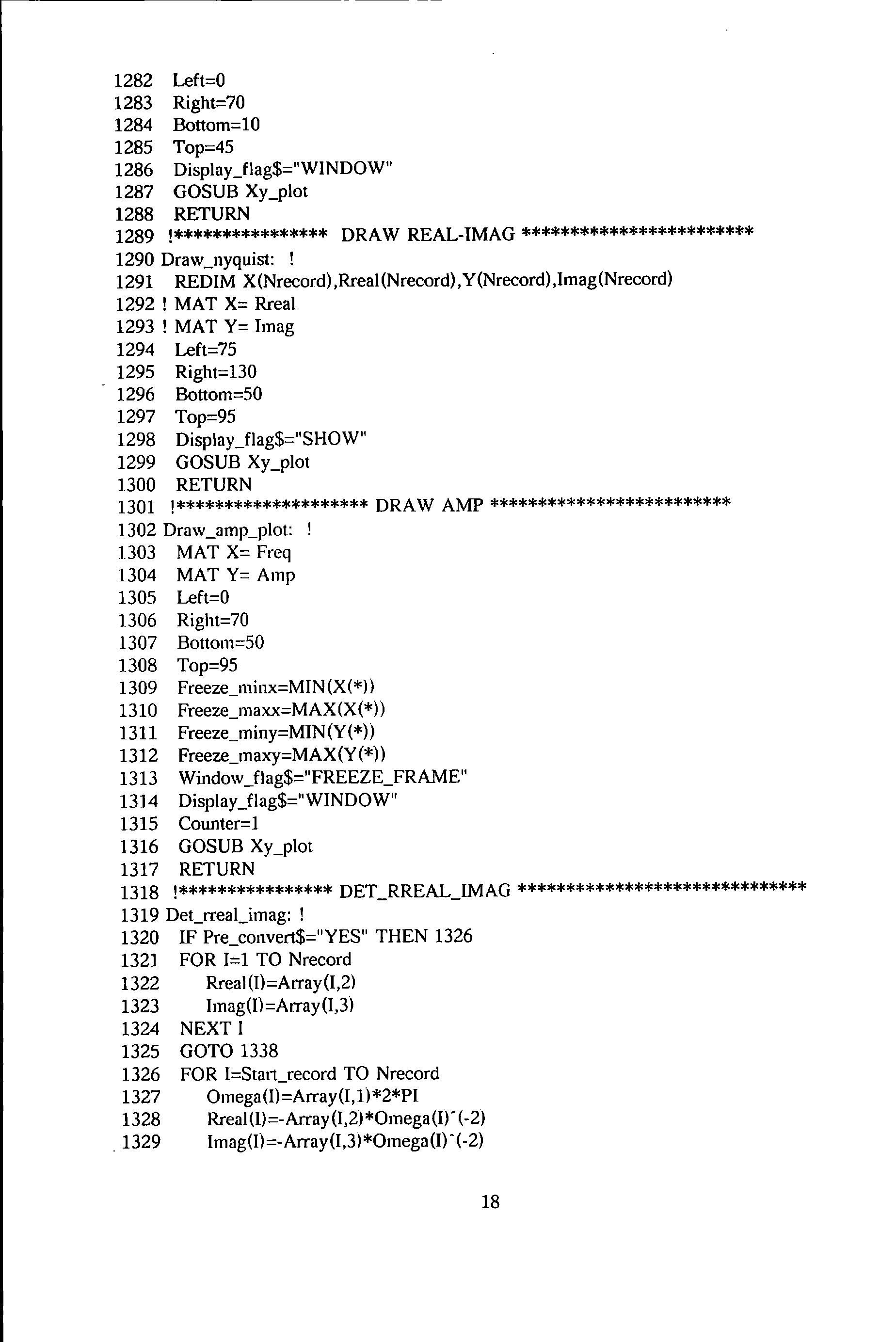
1282 Left=O 1283 Right=70 1284 Bottom=10 1285 Top=45 1286 Display_flag$=" WINDOW" 1287 GOSUB Xy_plot 1288 RETURN 1289 !**************** DRAW REAL-IMAG ************************ 1290 Draw_nyquist: ! 1291 REDIM X(Nrecord) ,Rreal(Nrecord), Y(Nrecord) ,Imag(Nrecord) 1292 ! MAT X= Rreal 1293 ! MAT Y= Imag 1294 Left=75 1295 Right=l30 1296 Bottom=SO 1297 Top=95 1298 Display_flag$="SHOW" 1299 GOSUB Xy_plot 1300 RETURN 1301 !******************** DRAW AMP ************************* 1302 Draw_amp_plot: 1303 MAT X= Freq 1304 MAT Y= Amp 1305 Left=O 1306 Right=70 1307 Bottom=SO 1308 Top=95 1309 Freeze_minx=MIN (X(*)) 1310 Freeze_maxx=MAX(X(*)) 1311 Freeze_miny=MIN(Y(*)) 1312 Freeze_maxy=MAX(Y(*)) 1313 Window_flag$="FREEZE_FRAME" 1314 Display_flag$="WINDOW" 1315 Counter=1 1316 GOSUB Xy_plot 1317 RETURN 1318 !**************** DET_RREAL_IMAG ****************************** 1319 Det_rreal_imag: ! 1320 IF Pre_convert$="YES" THEN 1326 1321 FOR 1=1 TO Nrecord 1322 Rreal (0=Array(I,2l 1323 Imag(l)=Array(I,3J 1324 NEXT I 1325 GOTO 1338 1326 FOR I=Stat1_record TO Nrecord 1327 Omega(I)=Array(I,1)*2*PI 1328 Rreal(l)=-Array(l,2)*0mega(Ir(-2) . 1329 lmag(ll=-Array(1,3)*0mega(I)"(-2) 18
1333 !

Array(I,3)=Imag(I)
NEXT I
1330 Array(I,2)=Rreai(I) 1331
1332
RESTRAINT
OMEGA=O
TO NEXT HIGHER FREQ VALUE" 1334 Rreal (l)=Rreal(2) 1335 Imag(1)=Imag(2) 1336 Array(1,2)=Array(2,2) 1337 Array(1,3)=Anay(2,3) 1338 RETURN 1339 !*************** *************************************** 1340 Yesno: ! 1341 PRINT Question$;"(Y)/N" 1342 Ask$="Y" 1343 INPUT Ask$ 1344 RETURN 1345 END 19
VALUES AT
EQUAL
Appendix 5.4 COMPARISON OF ERRORS IN THE MODAL PARAMETERS DETERMINED BY THE THREE METHODS
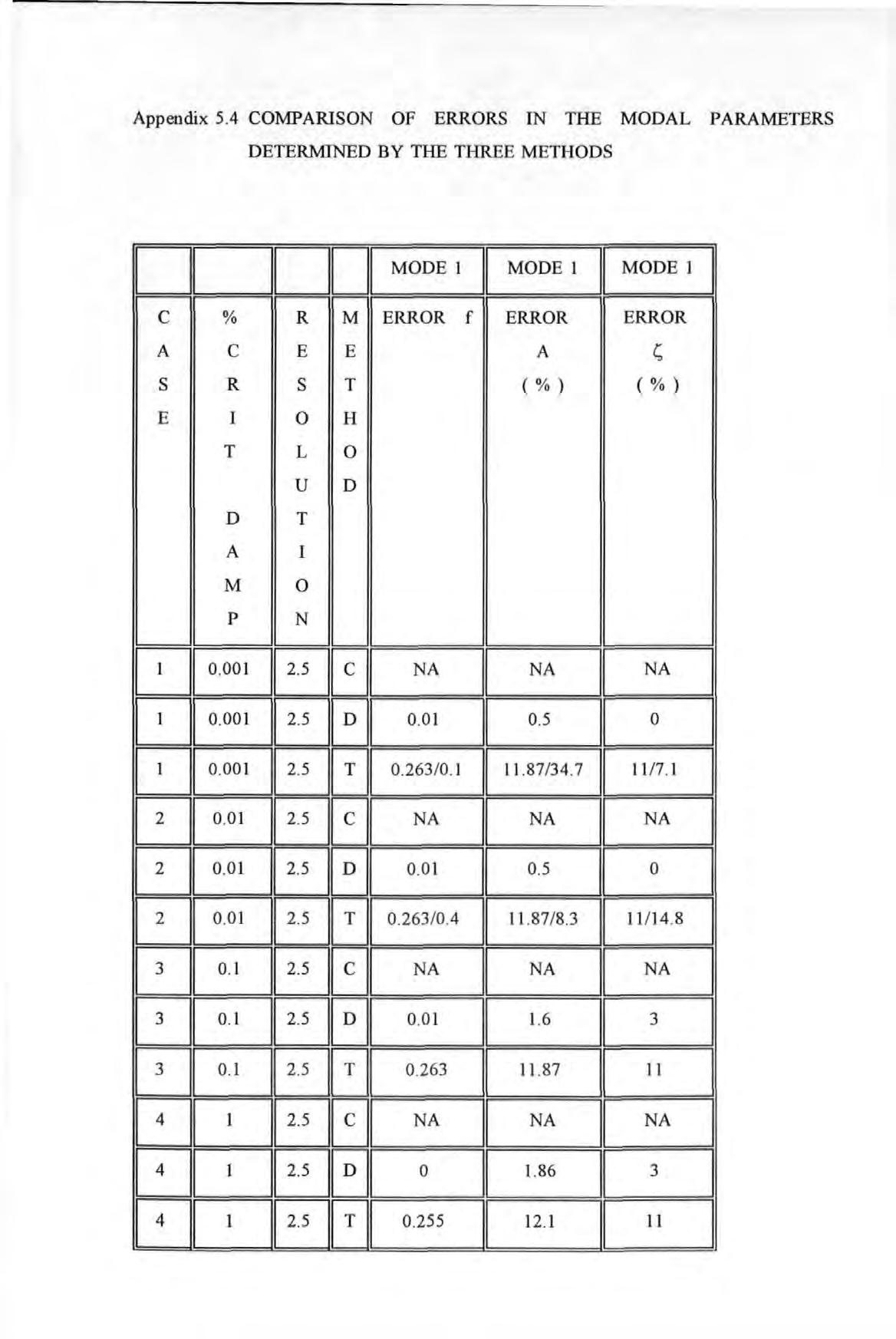
DDDDI MODE 1 11 MODEl 11 MODEl I c % R M ERROR f ERROR ERROR A c E E A s R s T (%) (%) E I 0 H T L 0 u D D T A I M 0 p N NA NA NA 0 01 0 5 0 0 .263/0 . 1 11.87/34 .7 11/7 . 1 NA NA 11 NA 0 01 0.5 I 0 0 .263 / 0.4 1l.87/8 .3 11 / 14 .8 NA NA NA 0 .01 1.6 3 0 263 11.87 I 11 NA NA NA 0 1.86 3 4 1 2.5 T 0 255 12 1 11
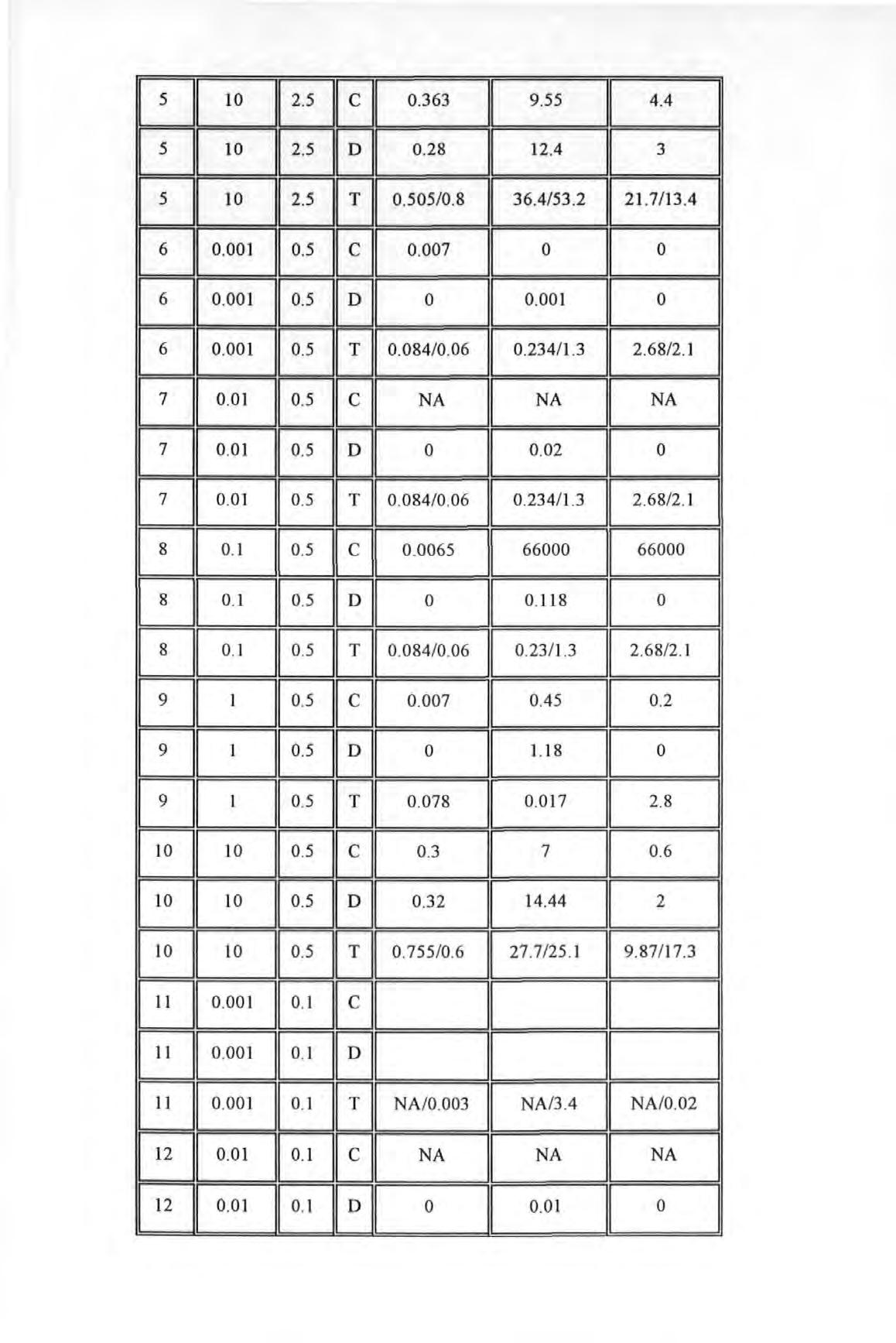
[] 10 0.363 9.55 4.4 5 10 2.5 0 .28 12.4 3 I 5 10 2.5 01 0 505/0 8 36.4/53 2 21.7/13.4 I 6 0.001 0 .5 0.007 I 0 0 I 0 I 0 001 0 0 084/0 06 0 .234/1 .3 2 .68/2 . 1 NA NA NA I 0 0 02 0 I 0 084/0 06 0 .234/1 3 2 68/2 1 I 0 0065 l 66000 l 66000 0 0 . 118 0 0 .084/0 .06 0 2 3/ 1 3 2.6 8/ 2 . 1 0 .007 0.45 0 2 0 1. 18 0 0.078 I 0 017 2 8 0 .3 7 0 .6 0.32 14.44 2 0 755 / 0 .6 27 7/25.1 9 87/17.3 NA/0 .003 NA/3.4 NA/0 .0 2 NA NA 11 NA 12 0 01 0.1 D 0 0 .01 I 0
D = DOBSON'S STRAIGHT LINE METHOD
T = AUTHOR'S METHOD
NA = NOT AVAILABLE OR NOT APPROPRIATE
f = RESONANT FREQUENCY IN Hz
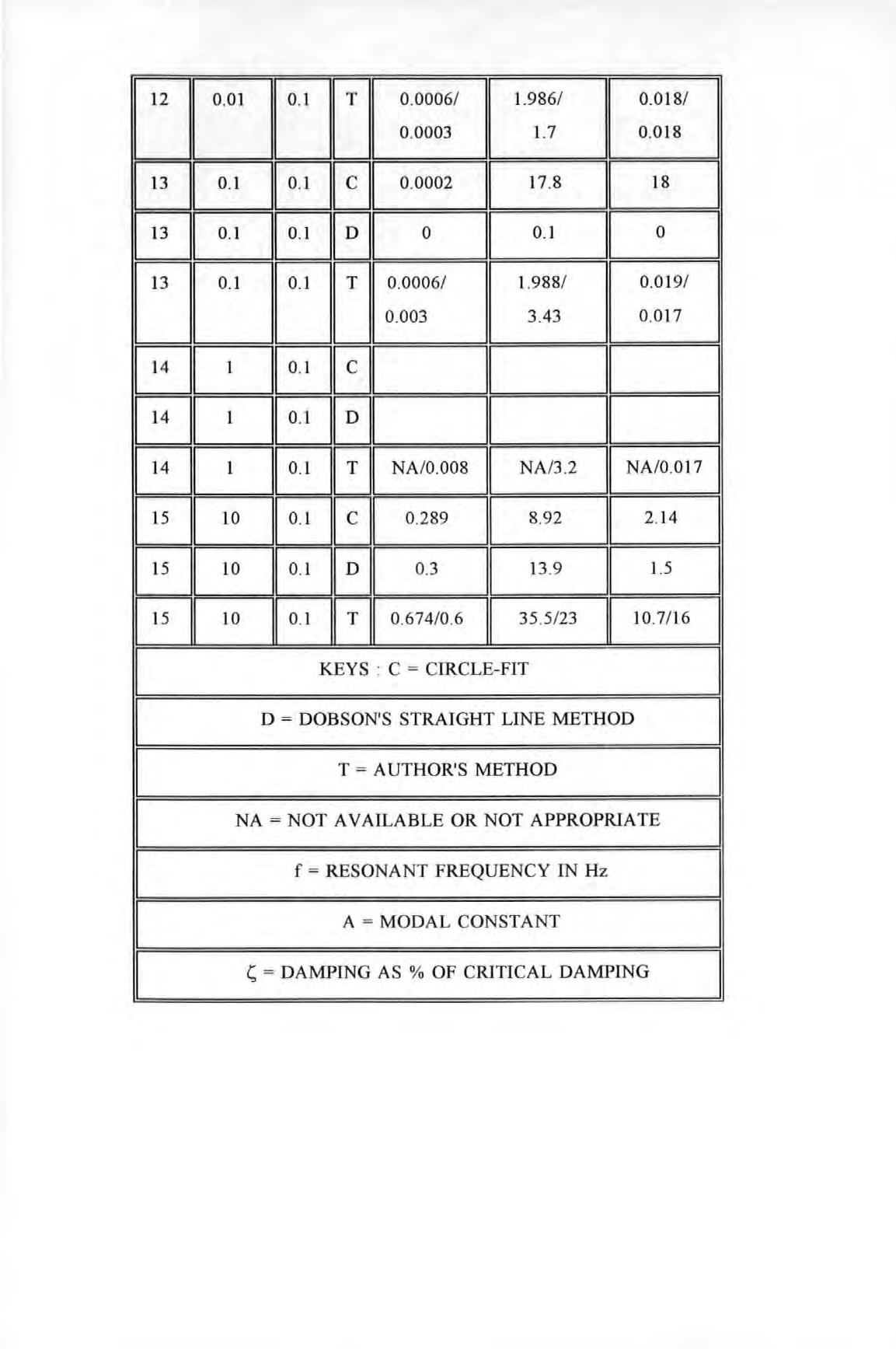
A = MODAL CONSTANT
l;: = DAMPING AS % OF CRITICAL DAMPING
0 .0006/ 0.018/ 0 .0003 0 018 7 0 0002 11 17 .8 11 18 I 0 11 0 . 1 11 0 I LJLJLIJ 0 0006/ 0 .019/ 0 003 0.017 3 1 0 1 01 NA /0.008 NA /3 2 NA/0 .017 10 0.289 I 8 .92 2.14 0.3 13.9 1.5 15 11 10 110 1 lfll 0 674/0 6 35 5/23 10 .7/16 KEYS : C = CIRCLE-FIT
LJLJLIJ
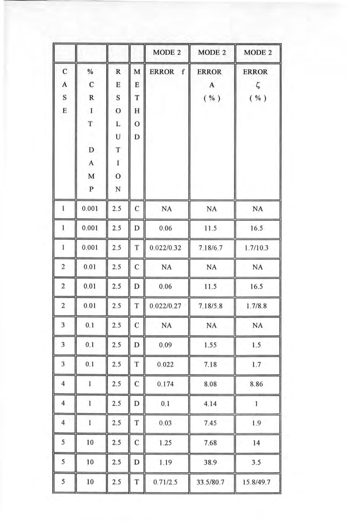
DDDDI MODE 2 11 MODE2 11 MODE2 I c % R M ERROR f ERROR ERROR A c E E A s R s T (%) (%) E I 0 H T L 0 u D D T A I M 0 p N NA NA NA I 0 06 11.5 16 5 I 0 02 2/0.32 7 18/ 6 7 1.7/10 3 I NA NA NA I D 0 .06 11.5 16 .5 0 022/0 27 I 7 18/5 8 1 7/8 8 NA NA NA 0 09 1.55 1.5 0 .022 7. 18 1.7 0 .174 8 08 8 .86 0 .1 4. 14 1 0 03 7.45 1.9 1.25 I 7 68 14 1.19 11 38 .9 11 3 .5 I 5 10 2.5 T 0 71/2 5 33 5/80 7 I 15 8/ 49 7 I
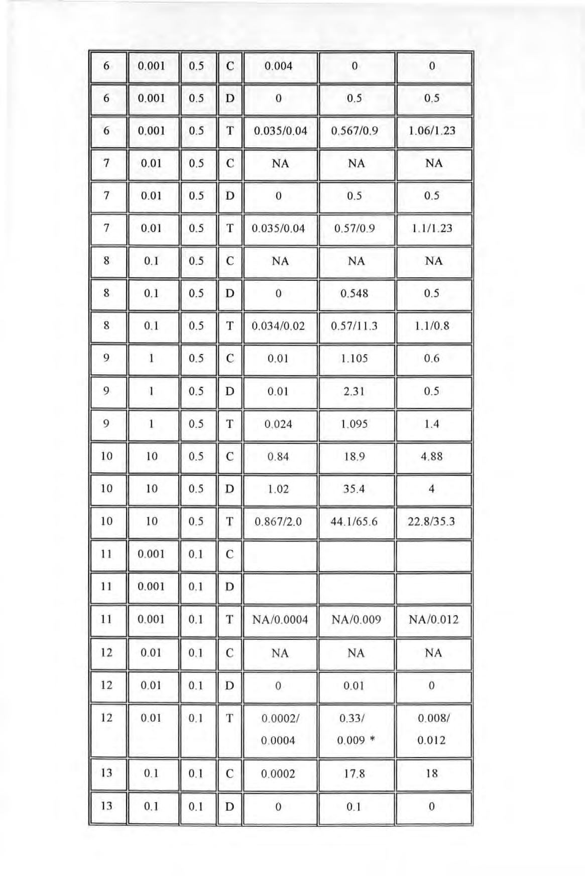
0 004 0 0 6 0.001 I o 5 0 0.5 0.5 6 0.001 0 5 0.035/0.04 0.567/0.9 1 06/1 23 NA NA NA 0 0.5 0 5 0 035/0.04 0 57/0 .9 1.1 /1.23 NA NA NA 0 0 .548 0 .5 0 .034/0 .02 0 57/11.3 1.1 /0.8 0 01 I 1 105 0 6 0 .01 2 .31 I 0 5 0 024 1.095 1.4 0 84 18 9 4 .88 1.02 35.4 I 4 0 . 86 7/2 .0 44 . 1/65 .6 22 .8/35 .3 NA / 0 .0004 NA / 0 009 NA/0 012 NA NA NA 0 0.01 0 LJLJLIJ 0 0002 / 0 33 / 0 008/ 0 0004 0.009 * 0 012 0 .0002 11 17 .8 11 18 I 13 0 1 0 1 D 0 0 1 I 0 I
KEYS : C = CIRCLE-FIT
D = DOBSON'S STRAIGHT LINE METHOD
T = AUTHOR'S METHOD
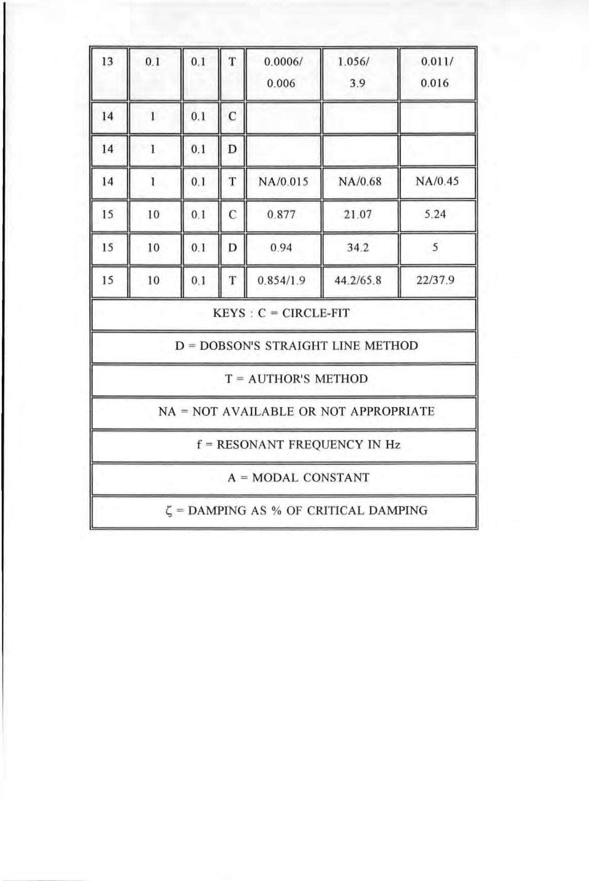
NA = NOT A VAILABLE OR NOT APPROPRIATE
f = RESONANT FREQUENCY IN Hz
A = MODAL CONSTANT
l;; = DAMPING AS % OF CRITICAL DAMPING
0.0006/ 0 011/ 0 006 0 016 9 I 11 NA/0.015 NA/0 68 NA/0.45 0 877 21 07 I 5 24 0 94 34 2 5 I 1 15 11 10 11 0 1 lfll 0 .854/1 .9 44 2/ 65 8 22/ 37 .9
LJLJLIJ
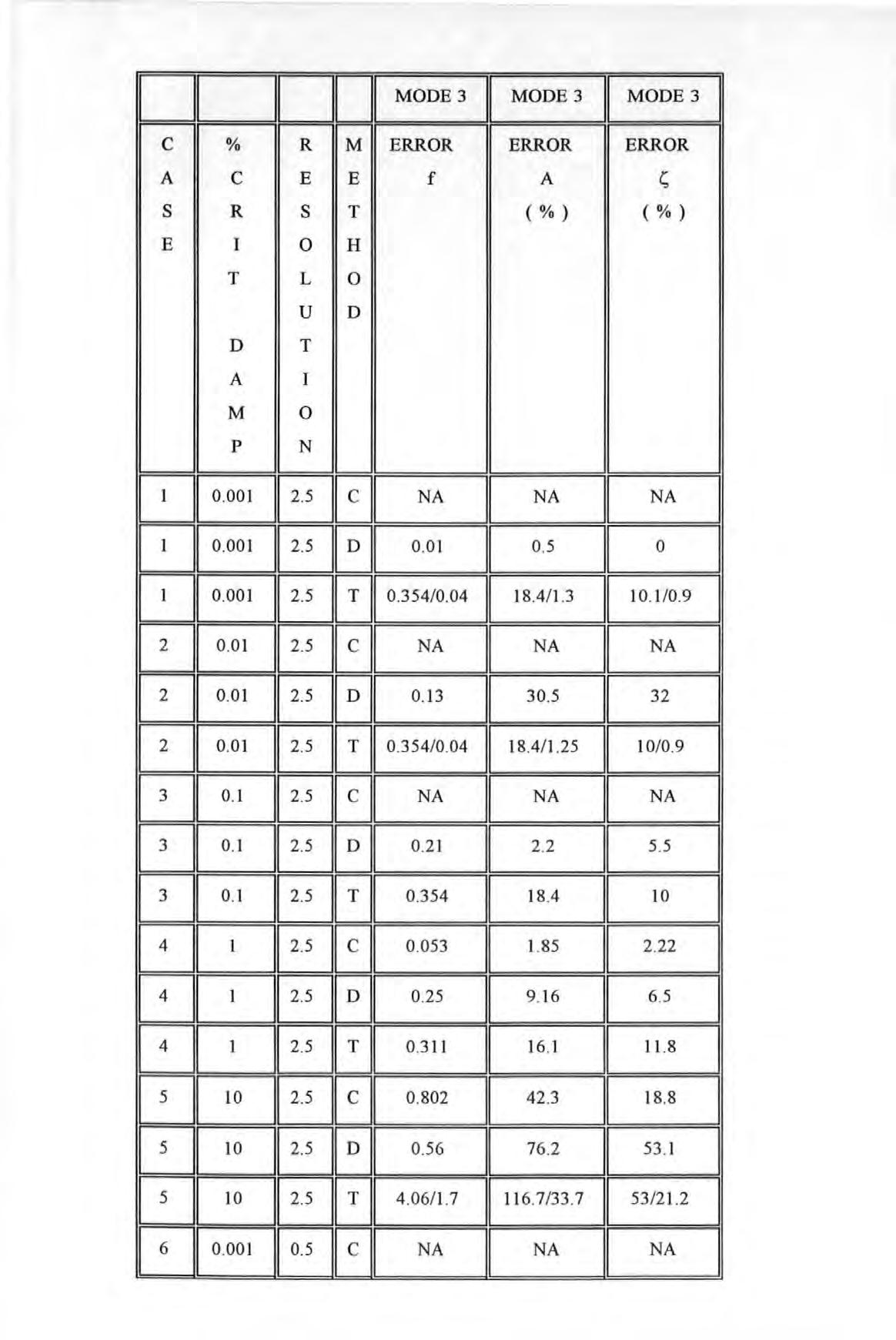
DDI MODE3 11 MODE3 11 MODE3 I c % R M ERROR ERROR ERROR A c E E f A s R s T (%) (%) E I 0 H T L 0 u D D T A I M 0 p N NA 11 NA NA 0.01 0 .5 0 0 .354/0.04 18 .4/ 1.3 10 . 1/0 .9 NA NA NA 0.13 30.5 32 0 354/0 04 18.4/ 1.25 10/ 0.9 NA NA NA 0 21 2 2 5 5 0 354 I 18.4 10 0 053 1.85 2 22 0 25 9 16 6 5 0 311 16 1 11.8 0 802 42 3 18 8 0 .56 76 .2 53 . 1 4 06/1.7 11 6 7/33. 7 53/21 .2 6 0 00 1 0 5 c NA NA NA
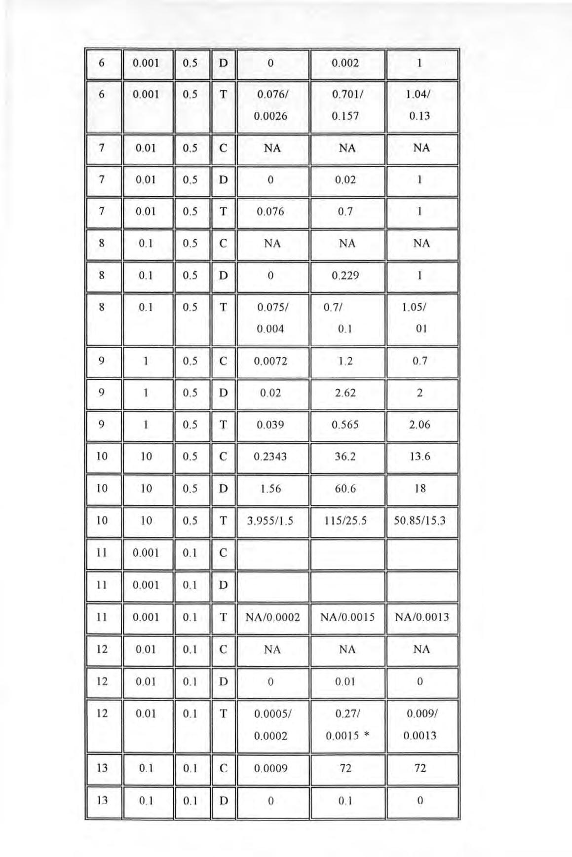
0 11 0.002 1 1 1
LJULIJ 0.076/ 0 701/ 0 0026 0.157 3 NA NA NA 0 0 02 I 0 076 0 7 1 NA NA NA 0 0.229 1 LJDLIJ 0 .075 / 0 004 01 0 0072 1.2 0 7 0 .02 2 .62 2 0 039 0 565 2 06 0 2343 36 2 I 13 6 1.56 60.6 18 3 .955/1 .5 I '15 /25.5 50 .85/15.3 NA/0 0002 NA / 0 .0015 NA / 0.0013 NA NA NA 0 0 01 0 LJLJEIJ 0 0005 / 0 27/ 0 009/ 0 0002 0 0015 * 0.0013 0 .0009 11 72 11 72 I 13 0 1 0 . 1 D 0 0 . 1 I 0 I
I
KEYS : C = CIRCLE-FIT
D = DOBSON1S STRAIGHT LINE METHOD
T = A UTHOR1S METHOD
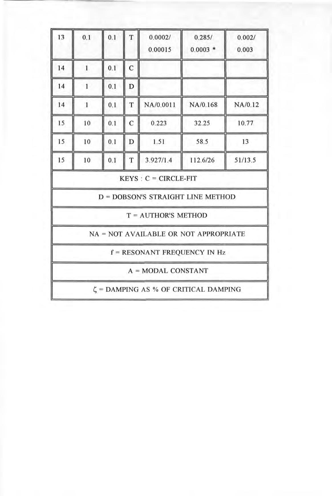
NA = NO T A V AILABLE OR NOT APPROPRIATE
f = RESONANT FREQUENCY IN H z
A = MODAL CONSTANT
l;; = DAMPING AS % OF CRITICAL DAMPING
0 .0002/ 0 .285 / 0 002/ 0 .00015 0 0003 * 0.003 1 1 I 11 NA/ 0 0011 11NA /0. 168 NA / 0. 12 I 0 223 1132.25 10.77 1.51 11 58 5 13 15 11 10 11 O l lfll 3.927/1.4 11 1 12 .6/26 51 / 13 5
LJLJLIJ
I
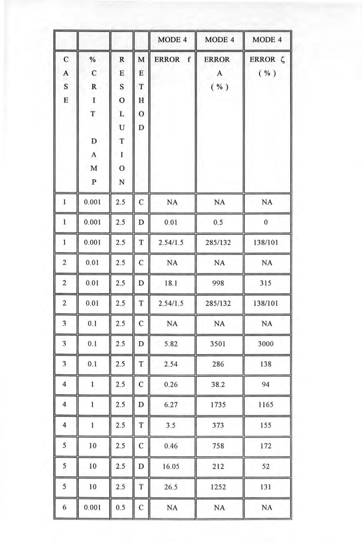
D I MODE 4 I MODE4 11 MODE4 I c % R M ERROR f ERROR ERROR A c E E A (%) s R s T (%) E I 0 H T L 0 u D D T A I M 0 p N NA 11 NA NA 0 .01 I 0 .5 0 2 54/ 1 5 285/132 138/101 NA NA NA 18 1 9 98 315 2 .54/ 1.5 285/132 138/ 101 NA NA NA 5.82 3501 3000 2 54 28 6 138 0.26 38 .2 94 I 6 27 1735 1165 3 5 373 155 5 I 0.46 758 172 5 16 .05 212 52 26 5 1252 131 6 0 001 0.5 c NA NA NA
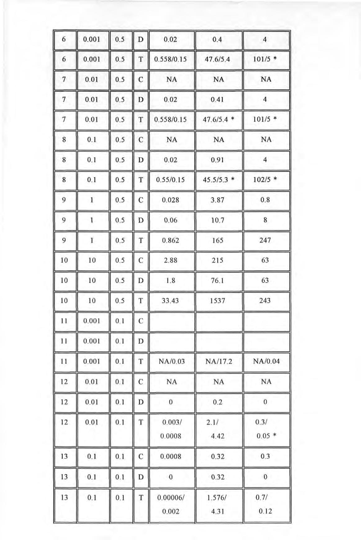
0 02 0.4 ll 4 0 558/0 15 47 6/5.4 101/5 * [JEJEJ01 NA NA NA 0.02 11 0 41 4 0.558/0 15 11 47 .6/5.4 * 101/5 * NA I NA I NA 0 .02 0.91 4 0 55/0 15 45 5/5 3 * 102/5 * 0.028 3 . 87 0.8 0 06 I 10 7 I 8 I 0. 862 165 247 2 .88 215 63 1.8 11 76 1 I 63 33 43 I 1537 11 243 NA / 0.03 NA / 17.2 NA / 0 04 NA 11 NA I NA 0 11 0. 2 11 0 LJEJLIJ 0 .003 / 2 . 1/ 0 0008 4.4 2 * 0 0008 11 0 3 2 0 3 I 0 11 0 .32 0 I 13 0. 1 0.1 T 0.00006/ 1.576/ 0 .7/ 0.00 2 4 .31 0 . 12
KEYS : C =CIRCLE-FIT
D = DOBSON'S STRAIGHT LINE METHOD
T = AUTHOR'S METHOD
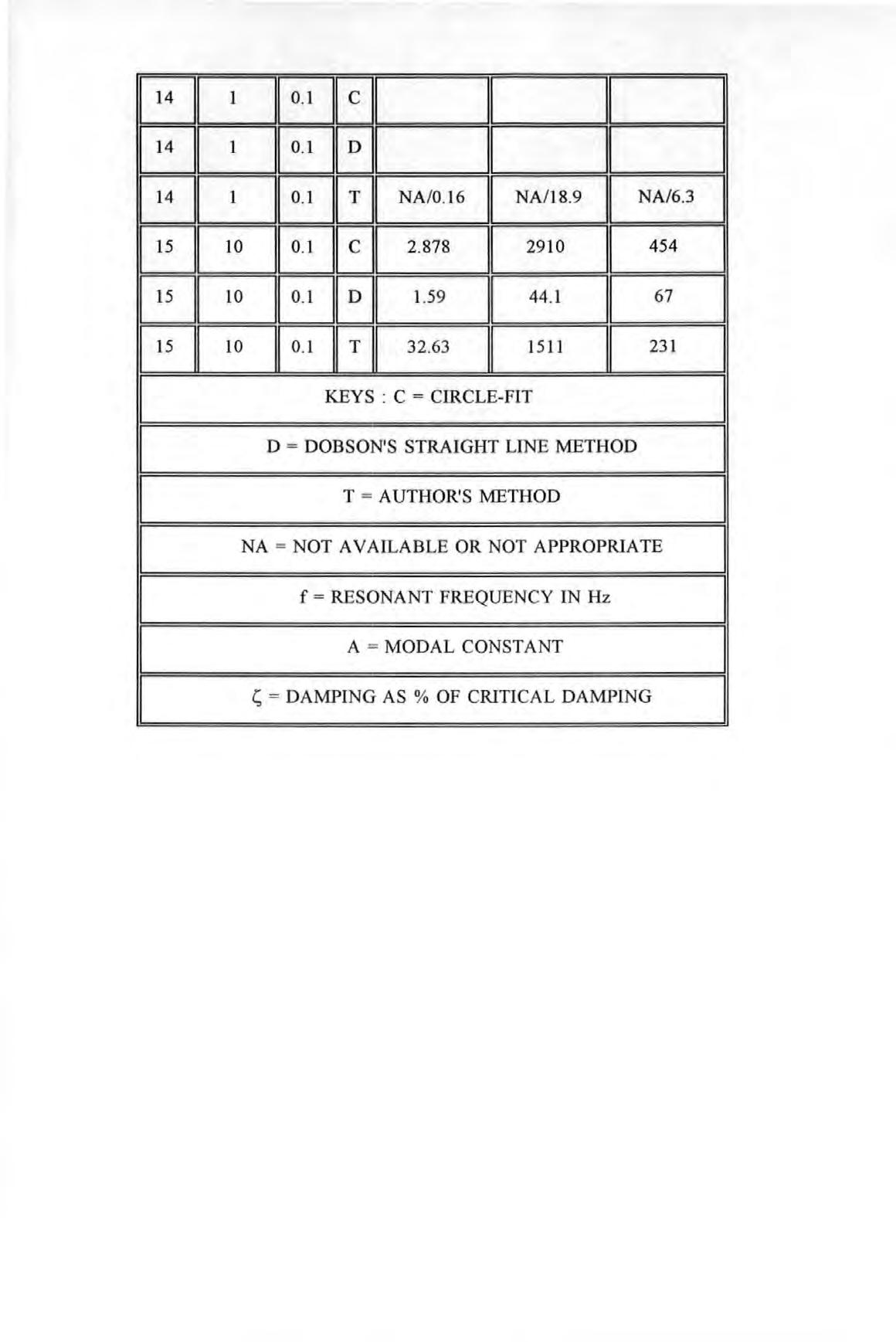
NA = NOT A VAILABLE OR NOT APPROPRlA TE
f = RESONANT FREQUENCY IN Hz
A = MODAL CONSTANT
= DAMPfNG AS % OF CRITICAL DAMPING
NA/0 . 16 I NA/18.9 NA/6.3 2 . 878 2910 454 1.59 44.1 67 15 11 10 110 1 lfll 32 63 1511 I 231
I
APPENDIX 6.3 ; LISTING OF THE SPATIAL PARAMETER EXTRACTION PROGRAM
10 ! NAME COMP _MCKl
20 ! THIS PROGRAM DERIVES THE M, C, K MATICES USING A COMPACT ALGORITHM
21 OPTION BASE 1
22 DIM Question$[80]
36 DUMP DEVICE IS 701
37 Question$="is this a re-run " 38 GOSUB Yesno 39 IF Ask$="N" THEN 40 Com_storage$="NO" 41 GOTO 44 42 END IF
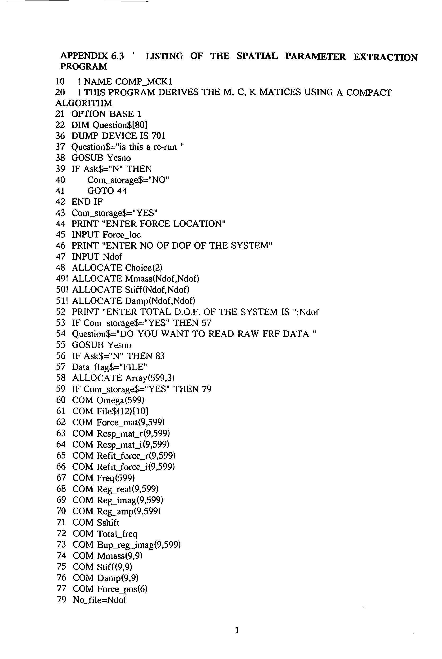
49! ALLOCATE Mmass(Ndof,Ndof)
50! ALLOCATE Stiff(Ndof,Ndof)
51! ALLOCATE Damp(Ndof,Ndof)
52 PRINT "ENTER TOTAL D.O.F. OF THE SYSTEM IS ";Ndof
53 IF Com_storage$="YES" THEN 57
54 Question$="DO YOU WANT TO READ RAW FRF DATA"
55 GOSUB Yesno
56 IF Ask$="N" THEN 83
57 Data_flag$="FILE"
58 ALLOCATE Array(599,3)
59 IF Com_storage$="YES" THEN 79
60 COM Omega(599)
61 COM File$(12)[10]
62 COM Force_mat(9,599)
63 COM Resp_mat_r(9,599)
64 COM Resp_mat_i(9,599)
65 COM Refit_force_r(9,599)
66 COM Refit_force_i(9,599)
67 COM Freq(599)
68 COM Reg_real(9,599)
69 COM Reg_imag(9,599)
70 COM Reg_amp(9,599)
71 COM Sshift
72 COM Total_freq
73 COM Bup_reg_imag(9,599)
74 COM Mmass(9,9)
75 COM Stiff(9,9)
76 COM Damp(9,9)
77 COM Force_pos(6)
79 No_file=Ndof
43 Com_storage$="YES" 44 PRINT "ENTER FORCE LOCATION" 45 INPUT Force_loc 46 PRINT "ENTER NO OF DOF OF THE SYSTEM" 47 INPUT Ndof 48 ALLOCATE Choice(2)
1

80 IF Com_storage$="YES" THEN 89 81 GOSUB Read_raw_frl 82 GOTO 86 83 GOSUB Read_modal_data 84 Data_flag$="MODALPARAM" 85 GOSUB Regeneration 86 IF Data_flag$="FILE" THEN 87 Total_freq=Nrecord 88 END IF 89 ALLOCATE X(Total_freq-Sshift) 90 ALLOCATE Y(Total_freq-Sshift) 91 Question$="DO YOU WANT TO SEE EACH FRF CURVES" 92 GOSUB Yesno 93 IF Ask$="N" THEN llO 94 FOR Dof=1 TO Ndof 95 FOR J=1 TO Total_freq-Sshift 96 X(J)=Freq(J) 97 IF Reg_amp(Dof,J)=O THEN 98 Reg_amp(Dof,J)=Reg_amp(Dof ,J+ 1) 99 END IF 100 Y(J)=20*LGT(ABS(Reg_amp(Dof,J))) 101 NEXT J 102 PRINT CHR$(12) 103 X_w1it$="Hz" 104 Y_unit$="dB" 105 GOSUB Plot_frl 106 PRINT "PRESS CONT" 107 PAUSE 108 NEXT Dof 109 ! DRAW FRF PLOT TO SELECT FREQ llO FOR J=1 TO Total_freq-Sshift 111 X(J)=Freq(J) 112 Y(J)=20*LGT(Reg_amp(Force_loc,J)) 113 NEXT J l14 GOSUB C01mect l15 REPEAT l16 PRINT CHR$(12) l17 PRINT "ENTER 1 IF ONLY THE REAL PARTS ARE USED" l18 PRINT "ENTER 2 IF ONLY THE IMAG PARTS ARE USED" 119 PRINT "ENTER 3 IF BOTH THE REAL AND IMAG PARTS ARE USED" 120 INPUT Assemble 121 UNTIL Assemble<=3 122 SELECT Assemble 123 CASE 1,2 124 Block_no=l 125 CASE 3 126 Block_no=2 127 END SELECT 2

YOU
ASSUME ZERO DAMPING" 129 Zero_damp$="NO" 130 GOSUB Yesno 131 IF Ask$="N" THEN 141 132 IF Block_no=2 THEN Block_no=1 ! SINCE IMAG PART CAN NOT BE USED 133 Zero_damp$="YES" 134 Zero$="ALREADY" 135 FOR Dof=1 TO Ndof 136 FOR 1=1 TO Total_freq-Sshift 137 Reg_imag(Dof))=O 138 NEXT J 139 NEXT Dof 140 GOTO 148 141 IF Zero$="ALREADY" THEN 142 FOR Dof=1 TO Ndof 143 FOR 1=1 TO Total_freq-Sshift 144 Reg_imag(Dof ))=Bup_reg_imag(Dof)) 145 NEXT J 146 NEXT Dof 147 END IF 148 PRINT CHR$(12) 149 GOSUB Pointer_table 150 X_unit$="Hz" _ 151 Y_w1it$="dB" 152 Dof=Force_loc ! TO PLOT FRF AT FORCING SITE FOR SELECT FREQ 153 GOSUB Plot_frf 154 DISP CHR$(129)&"SELECT FREQ POINTS" 155 Scan_type=1 156 GOSUB Freq_select 157 Question$=" DO YOU WANT TO DUMP THE GRAPH " 158 GOSUB Yesno 159 IF Ask$="N" THEN 161 160 DUMP GRAPHICS 161 GOSUB Assemble 162 DEALLOCATE Block(*) ,Block_vector(*) 163 ! DEALLOCATE Reg_real(*),Reg_imag(*) 164 GOSUB Solve_eq 165 GOSUB Fonning_mck 166 DEALLOCATE Coeff(*) 167 DEALLOCATE Sys_vector(*) 168 DEALLOCATE Mark_f_pointer(*) 169 DEALLOCATE Sel_freq(*) 170 DEALLOCATE Result_ vector(*) 171 DEALLOCATE Work_vector(*) 172 DEALLOCATE Work mat 1(*1 173 DEALLOCATE Work mat 2(*1 174 DEALLOCATE Work_mat_3(*) 175 Question$=" DO YOU WANT A RETRY WITH DIFFERENT DATA PTS" 3
128 Question$="DO
WANT TO
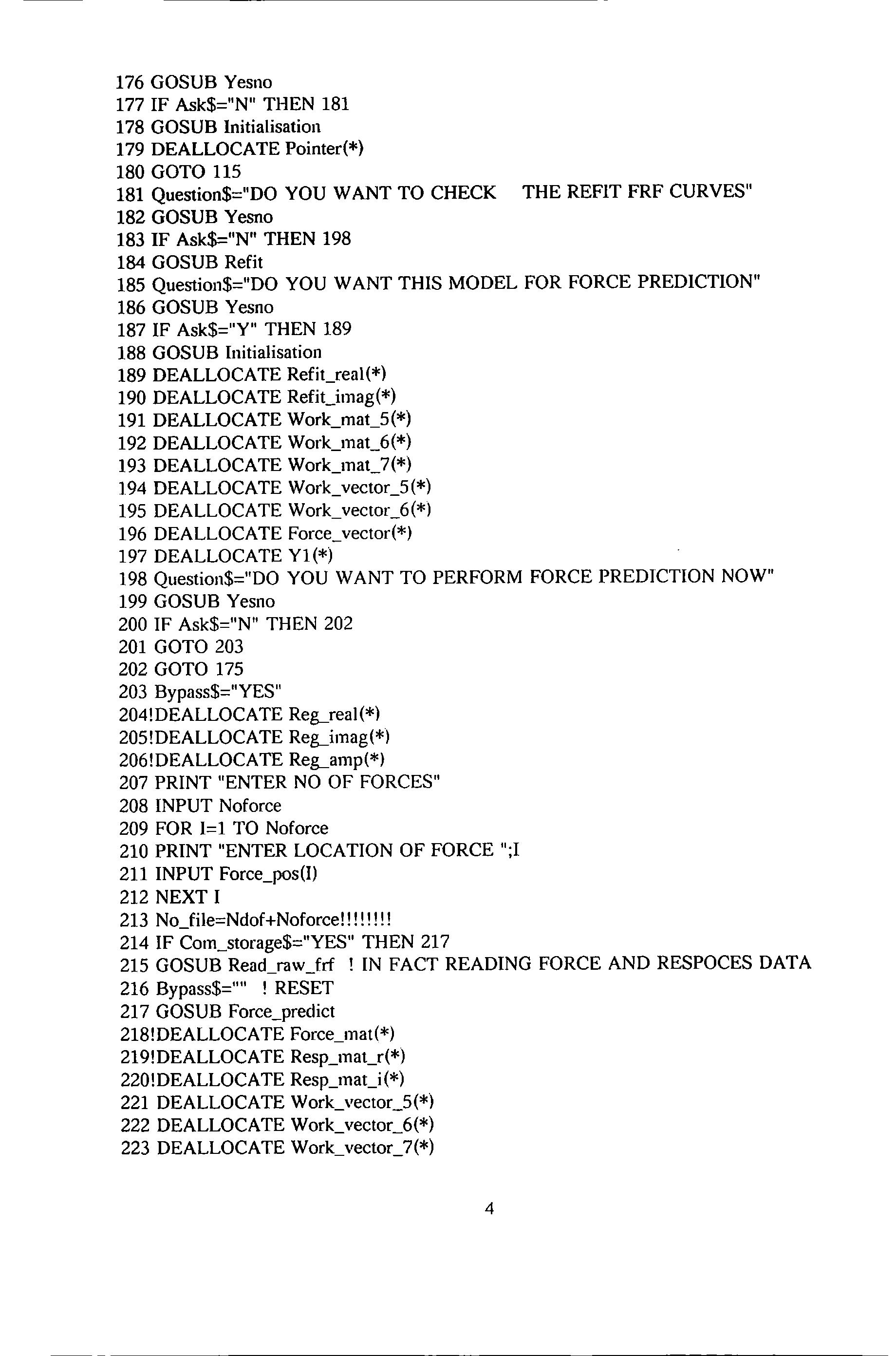
176 GOSUB Yesno 177 IF Ask$="N" THEN 181 178 GOSUB Initialisation 179 DEALLOCATE Pointer(*) 180 GOTO 115 181 Question$=" DO YOU WANT TO CHECK THE REFIT FRF CURVES" 182 GOSUB Yesno 183 IF Ask$="N" THEN 198 184 GOSUB Refit 185 Question$="DO YOU WANT THIS MODEL FOR FORCE PREDICTION" 186 GOSUB Yesno 187 IF Ask$="Y" THEN 189 188 GOSUB Initialisation 189 DEALLOCATE Refit_real(*) 190 DEALLOCATE Refit_imag(*) 191 DEALLOCATE Work_mat_5(*) 192 DEALLOCATE Work mat 6(*) 193 DEALLOCATE Work_mat_7(*) 194 DEALLOCATE Work_vector_5(*) 195 DEALLOCATE Work_vector_6(*) 196 DEALLOCATE Force_vector(*) 197 DEALLOCATE Y1(*) 198 Question$="DO YOU WANT TO PERFORM FORCE PREDICTION NOW" 199 GOSUB Yesno 200 IF Ask$="N" THEN 202 201 GOTO 203 202 GOTO 175 203 Bypass$="YES" 204!DEALLOCATE Reg_real(*) 205!DEALLOCATE Reg_imag(*) 206!DEALLOCATE Reg_amp(*) 207 PRINT "ENTER NO OF FORCES" 208 INPUT Noforce 209 FOR 1=1 TO Noforce 210 PRINT "ENTER LOCATION OF FORCE ";I 211 INPUT Force_pos(I) 212 NEXT I 213 No_file=Ndof+Noforce!!!!!!!! 214 IF Com_storage$="YES" THEN 217 215 GOSUB Read_raw_frf ! IN FACT READING FORCE AND RESPOCES DATA 216 Bypass$='"' ! RESET 217 GOSUB Force_predict 218!DEALLOCATE Force mat(*) 219!DEALLOCATE Resp_mat_r(*) 220!DEALLOCATE Resp_mat_i (*) 221 DEALLOCATE Work_vector_5(*) 222 DEALLOCATE Work_vector_6(*) 223 DEALLOCATE Work_vector_7(*) 4
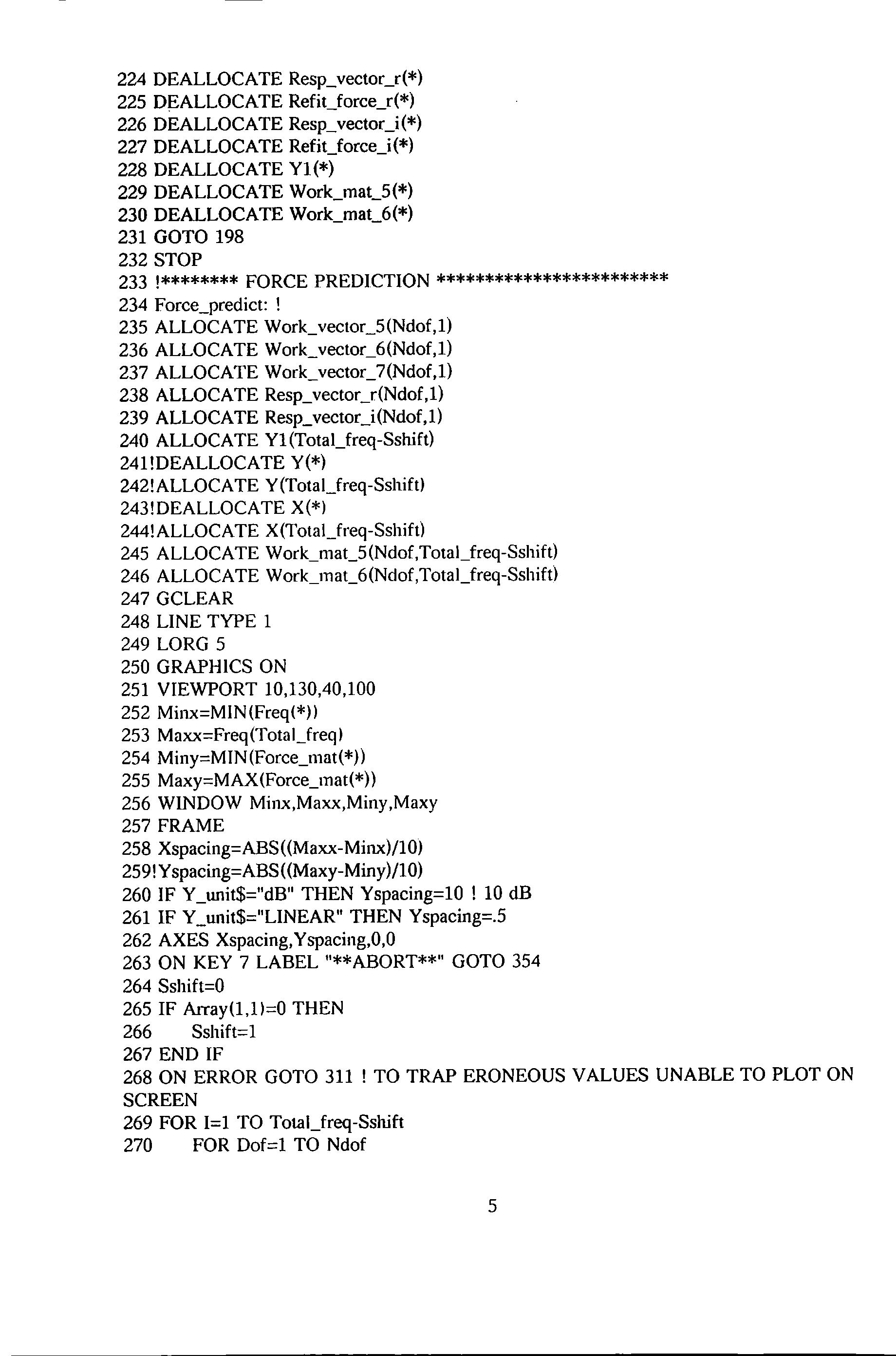
224 DEALLOCATE Resp_vector_r(*) 225 DEALLOCATE Refit_force_r(*) 226 DEALLOCATE Resp_vector_i(*) 227 DEALLOCATE Refit_force_i(*) 228 DEALLOCATE Y1 (*) 229 DEALLOCATE Work mat 5(*) 230 DEALLOCATE Work mat 6(*) 231 GOTO 198 232 STOP 233 !******** FORCE PREDICTION ************************ 234 Force_predict: ! 235 ALLOCATE Work_vector_5(Ndof,l) 236 ALLOCATE Work_vector_6(Ndof,l) 237 ALLOCATE Work_vector_7(Ndof,l) 238 ALLOCATE Resp_vector_r(Ndof,1) 239 ALLOCATE Resp_vector_i(Ndof,l) 240 ALLOCATE Y1 (Total_freq-Sshift) 241!DEALLOCATE Y(*) 242!ALLOCATE Y(Total_freq-Sshiftl 243!DEALLOCATE X(*l 244!ALLOCATE X(Total_freq-Sshift) 245 ALLOCATE Work_mat_5(Ndof,Total_freq-Sshift) 246 ALLOCATE Work_mat_6(Ndof,Total_freq-Sshift) 247 GCLEAR 248 LINE TYPE 1 249 LORG 5 250 GRAPHICS ON 251 VIEWPORT 10,130,40,100 252 Minx=MIN(Freq(*)) 253 Maxx=Freq(Total_freql 254 Miny=MIN(Force_mat(*)) 255 Maxy=MAX(Force_mat(*)) 256 WINDOW Minx,Maxx,Miny,Maxy 257 FRAME 258 Xspacing=ABS((Maxx-Minx)/10) 259!Yspacing=ABS((Maxy-Miny)/10) 260 IF Y_unit$="dB" THEN Yspacing=10 ! 10 dB 261 IF Y_unit$="LINEAR" THEN Yspacing=.5 262 AXES Xspacing,Yspacing,O,O 263 ON KEY 7 LABEL "**ABORT**" GOTO 354 264 Sshift=O 265 IF Array(l,li=O THEN 266 Sshift=1 267 END IF 268 ON ERROR GOTO 311 ! TO TRAP ERONEOUS VALUES UNABLE TO PLOT ON SCREEN 269 FOR 1=1 TO Total_freq-Sshift 270 FOR Dof=1 TO Ndof 5
271 Resp_vector_r(Dof ,1)=Resp_mat_r(Dof ,I) 272 Resp_vector_i(Dof,l) =Resp_mat_i (Dof,I) 273 NEXT Dof 274 IF Freq(I)=O THEN Freq(I)=Freq(l+1) 275 Oomega=2*PI*Freq (I) 276 ! MAT Work_mat_5= Stiff*(-(2*PI*Freq(l))"(-2)) 277 MAT Work_mat_6= Work_mat_5+Mmass 278 MAT Work_mat_5= (-Oomega·2)*Mmass 279 MAT Work_mat_6= Work_mat_5+Stiff 280 MAT Work_vector_5= Work_mat_6*Resp_vector_r 281 MAT Work_mat_5= Damp*(-Oomega) 282 MAT Work_vector_6= Work_mat_5*Resp_vector_i 283 MAT Work_vector_7= Work_vector_5+Work_vector_6 284 FOR Dof=1 TO Ndof 285 DISP CHR$(129)&"REFIT CALCULATION FOR FREQ PT ";I 286 Refit_force_r(Dof,O=Work_vector_7(Dof,1) 287 NEXT Dof 288 MAT Work_vector_5= Work_mat_6*Resp_vector_i 289 MAT Work_vector_6= Work_mat_5*Resp_vector_r 290 MAT Work_vector_7= Work_vector_5-Work_vector_6 291 FOR Dof=l TO Ndof 292 DISP CHR$(129)&"REFIT CALCULATION FOR FREQ PT ";I 293 Refit_force_i (Dof,I)=Work_vector_7(Dof,l) 294 NEXT Dof 295 Refit_force_am p=(Refit_force_i (Force_loc,I) ·2+Refit_force_r(Force_loc, I) ·2)· 0 5 296 Remainder=! MOD 4 297 IF Remainder>=] THEN 298 IF Force_mat(Force_locoli=O THEN 299 ! MOVE Freq(l)oMiny 300 ! GOTO 234 301 ! END IF 302 MOVE Freq (I) ,ABS(Force_mat(Force_loc,I)) 303 LABEL "0" 304 IF Refit_force(Force_locoi)=O THEN 305 ! MOVE Freq(II,Miny 306 ! GOTO 240 307 END IF 308 MOVE Freq(I),ABS(Refit_force_amp) 309 LABEL"+" 310 END IF 311 NEXT I 312 OFF ERROR 313 FOR Dof=l TO Ndof 314 Eerror=O ! RESET 316 FOR 1=1 TO Total_freq-Sshift 317 X(Il=Freq(l) 318 IF Force_mat(Dof,I)=O THEN 319 Y(Il=20*LGT(l.E-10) 6

320 ! GOTO 316 321! END IF 322 Y (I) =(ABS (Force_mat(Dof, I))) 323 Refit_force_amp=(Refit_force_i(Dof,I).2+Refit_force_r(Dof,I).2)·.s
Y1 (I)=(ABS(Refit_force_amp))
·Rms=((Refit_force_amp-Force_mat(Dof,I) )"2)" .5 326 Eerror=Eerror+Rms 327 NEXT I 328 Eerror=Eerror!fotal_freq 329 PRINTER IS 701 330 PRINT "RMS ERROR FOR DOF =";Dof;" IS =";Eerror 331 PRINTER IS l 333 PRINT CHR$(12) 334 GCLEAR 335 Miny=O ! Mlny=MIN(Y1(*),Y(*)) 336 Maxy=20 ! Maxy=MAX(Y(*),Yl(*)) 337 ! Maxy=MAX(Y(*),Y1(*)) 338 Overlay$="YES" 339 X_unit$="Hz" 340 Y unit$="LlNEAR" 341 Frame$="0VERLA Y" 342 Overlay$="YES" 343 GOSUB Plot_frf 344 Question$=" DO YOU WANT TO DUMP GRAPH " 345 GOSUB Yesno 346 IF Ask$="N" THEN 348 347 DUMP GRAPHICS 348 NEXT Dof 349 LlNE TYPE 1 350 FOR J=l TO Total_freq-Sshift 351 X(Jl=Freq(Jl 352 Y (J l=20*LGT(Reg_amp(Force_Ioc,J)) 353 NEXT J 354 RETURN 355 ! ****************** QUIT ************************ 356 Quit: ! 357 Quit$="YES" 358 RETURN 359 !************* INITIALISATION *********************** 360 Initialisation: ! 361 FOR I=l TO Ndof 362 FOR J=l TO Ndof 363 Mmass(I,Jl=O 364 Stiff(I,JJ=O 365 Damp(l,J)=O 366 NEXT J 367 NEXT I 368 RETURN
324
325
369 !******************REFIT***************************** 370 Refit: ! 371 ALLOCATE Refit_real(Ndof,Total_freq) 372 ALLOCATE Refit_imag(Ndof,Total_freq) 373 ALLOCATE Work_mat_5(Ndof,Ndof) 374 ALLOCATE Work_mat_6(Ndof,Ndof) 375 ALLOCATE Work_mat_7(Ndof,Ndof) 376 ALLOCATE Work_vector_5(Ndof,l) 377 ALLOCATE Work_vector_6(Ndof,1) 378 ALLOCATE Force_vector(Ndof,1) 379 ALLOCATE Yl (Total_freq-Sshift) 380 ! SET UP FORCE VECTOR 381 FOR Dof=l TO Ndof 382 IF Dof=Force_loc THEN 383 Force_vector(Dof,1)=1 384 ELSE 385 Force_ vector(Dof, 1) =0 386 END IF 387 NEXT Dof 388 GCLEAR 389 LINE TYPE 1 390 LORG 5 391 GRAPHICS ON 392 VIEWPORT 10,130,40,100 393 WINDOW Minx.Maxx,Miny,Maxy 394 FRAME 395 AXES Xspacing,Yspacing,O,O 396 ON KEY 5 LABEL "**ABORT**" GOTO 474 397 FOR 1=1 TO Total_freq-Sshift 398 Oomega=2*PI*Freq(l) 399 MAT Work_mat_5= (-Oomega"2)*Mmass 400 MAT Work_mat_6= Work_mat_S+Stiff 401 MAT Work_mat_5= INV(Work_mat_6) 402 MAT Work_mat_7= Work_mat_S*Damp 403 MAT Work_mat_S= Damp*Work_mat_7 404 MAT Work_mat_7= Work_mat_S*(Oomega"2) 405 MAT Work_mat_5= Work_mat_7+Work_mat_6 406 MAT Work_mat_7= INV(Work_mat_S) 407 MAT Work_vector_S= Work_mat_7*Force_vector 408 FOR Dof=1 TO Ndof 409 DISP CHR$(129l&"REFIT CALCULATION FOR FREQ PT ";I 410 Refit_real (Dof,Il=Work_vector_5(Dof,1 l 411 NEXT Dof 412 MAT Work_mat_5= INV(Work_mat_6) 413 MAT Work_mat_7= (-0omega)*Work_mat_5 414 MAT Work_mat_5= Work_mat_7*Damp 415 MAT Work_vector_6= Work_mat_5*Work_vector_5 416 FOR Dof=l TO Ndof 8
417 Refit_imag(Dof,l)=Work_vector_6(Dof,1) 418 NEXT Dof 419 Remainder=I MOD 4 420 IF Remainder>=1 THEN 421 MOVE Freq(I),20*(LGT(Reg_amp(Force_Ioc,I))) 422 LABEL "." 423 Refit_am p=(Refit_real (Force_Ioc,I) "2+Refit_imag(Force_Ioc,I) "2) •. 5 424 MOVE Freq(I),20*LGT(Refit_amp) 425 LABEL"+" 426 END IF 427 NEXT I 428 FOR Dof=1 TO Ndof 429 Eerror=O 430 Sumsq=O 432 FOR 1=1 TO Total_freq-Sshift 433 X(I)=Freq(I) 434 IF Reg_amp(Dof,l)=O THEN 435 Reg_amp(Dof,O=Reg_amp(Dof,I+ l) 436 END IF 437 Y(I)=20*LGT(Reg_amp(Dof,l)) 438 Refit_amp=(Refit_real (Dof ,I) "2+Refit_imag(Dof ,1) "2) · .5 439 Y1 (1)=20*LGT(Refit_amp) 440 Rms=( (Refit_amp-Reg_amp(Dof,l) )"2) 441 Sumsq=Reg_amp(Dof,I)"2+Sumsq 442 Eerror=Eerror+Rms 443 NEXT I 444 Eerror=1-(Eerror/Sumsq) ·.5 445 PRINTER IS 701 446 PRINT "Q FACTOR FOR DOF =";Dof;" IS =";Een·or 447 PRINTER IS 1 448 PRINT CHR$(12) 449 GCLEAR 450 Miny=MlN(Y1(*),Y(*)) 451 Maxy=MAX(Y(*),Y1(*)) 452 Overlay$="YES" 453 LINE TYPE l 454 X_unit$="Hz" 455 Y_unit$=" dB" 456 GOSUB Plot_frf 457 LINE TYPE 4 458 MAT Y= Y1 459 Frame$="0VERLA Y" 460 Overlay$="YES" 461 X_unit$="Hz" 462 Y_unit$=" dB" 463 GOSUB Plot_frf 464 Question$=" DO YOU WANT TO DUMP GRAPH " 465 GOSUB Yesno 9
466 IF Ask$="N" THEN 468 467 DUMP GRAPHICS . 468 NEXT Dof 469 LINE TYPE 1 470 FOR J=1 TO Total_freq-Sshift 471 X(J)=Freq(J)
IF Bypass$="YES" THEN 503
! ALLOCATE File$(Ndof+1)[10]
FOR Dof=1 TO No_file
PRINT "ENTER DATA FILE NAME FOR DOF ";Dof
OUTPUT 2;"K"&CHR$(255)&CHR$(631;
473
474 RETURN 475 ! ****************
****************************** 476 Yesno: ! 477 OUTPUT
478
479 Ask$="UNSET" 480 REPEAT 481
482
483
Yes 484 UNTIL
485 Nno: ! 486 Ask$="N" 487 GOTO 490 488 Yes: ' 489 Ask$="Y" 490 OFF CYCLE 491 OFF KEY 492 OUTPUT 2;"K"; 493 RETURN 494 ! ****************** ATTENTION *********************** 495 Attention: ! 496 Bbeep: 497 BEEP 500,1 498 RETURN 499! **********************READ
DATA************** 500 Read_raw_frf:
501
502
503
505
506
507 NEXT Dof 508 OUTPUT
509 Question$="BY
510 GOSUB Yesno 511
512 Bypasscale$="YES" 513 GOTO
10
472 Y(J)=20*LGT(Reg_amp(Force_loc,J))
NEXT J
YESNO
2;"K";
ON CYCLE 3 GOSUB Attention
DISP CHR$(129)&Question$;" (Y)/N"
ON KEY 5 LABEL "NO" GOTO Nno
ON KEY 9 LABEL "(YES)" GOTO
Ask$="Y" OR Ask$="N"
RAW FRF
!
504
INPUT File$(Do0
2;"K";
PASS SCALING "
IF Ask$="Y" THEN
526
514 ELSE
515 Bypasscale$="NO"
516 GOTO 518
517 END IF
518 Question$=" MULTIPLY fjw)"2 (Y) OR/ DIVIDE Gw)"2 (N)"
519 GOSUB Yesno
520 IF Ask$="Y" THEN
521 Power=2
522 GOTO 526
523 ELSE
524 Power=-2
525 END IF
526 FOR Dof=1 TO No_file
527 DISP "READING RAW FRF DATA FROM FILE ";Dof
528 GOSUB Read_file
529 NEXT Dof
530 RETURN
531 !***************READ FILE****************************
532 Read_file: !
533 DO$=":HP9121,700,0"
534 Dl$=":HP9133,700,0"
535!PRINT "ENTER DATA FILE NAME FOR DOF ";Dof
536!INPUT File$
537 ASSIGN @File TO File$(Dof)&Dl$
538 ENTER @File;Nrecord,Dummy,Dummy
539 Total_freq=Nrecord
540 REDIM Array(Nrecord,3)
541 ENTER @File;Array(*)
542 ASSIGN @File TO*
543 Sshift=O
544 IF Bypass$="YES" THEN 568
545 IF Array(l,l)=O THEN
546 Sshift=1
547 END IF
548 FOR Data_pt=1 TO Nrecord-Sshift
549 DISP "COUNT DOWN ";Nrecord-Sshift-Data_pt
550 Freq (Data_pt)=Array(Data_pt+Sshift, 1)
551 SELECT Bypasscale$
552 CASE "YES"
553 Sscale=l
554 CASE "NO" 555 Sscale=-1 *(2*PI*Freq(Data_pt) )"(Power)
556 CASE ELSE
557 PRINT "SCALING FACTOR NOT CLEARLY DEFINED!!!!"
558 PRINT "please check program line 543"
559 BEEP 560 PAUSE 561 END SELECT
11
562 Reg_real(Dof,Data_pt)=Array(Data_pt+Sshift,2)*Sscale 563 Reg_imag(Dof.Data_pt)=A1Tay(Data_pt+Sshift,3)*Sscale 564 Bup_reg_imag(Dof,Data_pt)=Reg_imag(Dof,Data_pt)*Sscale 565 Reg_amp(Dof,Data_pt)=(Reg_real(Dof,Data_pt)"2+Reg_imag(Dof,Data_pt)"2)".5 566 NEXT Data_pt 567 GOTO 590 568 FOR Data_pt=l TO Nrecord-Sshift 569 DISP "COUNT DOWN ";Nrecord-Sshift-Data_pt 570 Freq(Data_pt)=An·ay(Data_pt+Sshift,l) 571 SELECT Bypasscale$ 572 CASE "YES" 573 Sscale=l 574 CASE "NO" 575 Sscale=- 1*(2*PI*Freq (Data_pt) )"(Power) 576 CASE ELSE 577 PRINT "SCALING FACTOR NOT CLEARLY DEFINED!!!!" 578 PRINT "please check program line 543" 579 BEEP 580 PAUSE 581 END SELECT 582 IF Dof>=Nclof+l THEN 583 Force_pointer=Dof-Nclof 584 Force_mat (Force_pos (Force_poin ter), Da ta_pt) =(Array (Data_pt +Ssh ift,2) "2+Array(Data_pt+ Sshift,3r2r .5 585 ELSE 586 Resp_mat_r{Dof,Data_pt)=Array(Data_pt+Sshift,2)*Sscale 587 Resp_mat_i (Dof ,Data_pt) =Array(Data_pt +Ss hi ft,3) *Sscale 588 END lF 589 NEXT Data_pt 590 RETURN 591 ! ************ READ CURSOR *********************** 592 Reacl_cursor: ! 593 REPEAT 594 ON KNOB .01,1 GOSUB Spin 595 ON KEY 5 LABEL "*MARK*",l GOSUB Mark 596 UNTIL Mark$="YES" 597 PEN 1 598 LINE TYPE 1 599 RETURN 600 !********** MARK ******************************** 601 Mark: ! 602 Mark$="YES" 603 SELECT Scan_type 604 CASE 1 605 MOVE X(Counter).Y(Counter) 606 LABEL Freq_count 607 Mark_f_pointer(Freq_count)=Counter 12
(Counter)
611 Choice( Choose_scale) =Y_position
645 SET ECHO X(Cmmter),Y(Cowuer) 646 SELECT Scan_type
2
ON ERROR GOTO 657! TO TRAP ERROR IF ONLY ONE CURVE
";"Y1=";Y1(Counter)
SELECT 654 DISP CHR$(129l&"CURSOR FREQ "&VAL$(Freq(Counter))&" HZ";" ";"Y="; Y(Counter)
608 Sel_freq(Freq_count)=Freq
609 GOTO 618 610 CASE 2
CLIP
CLIP ON 616 GOTO
END SELECT 618 RETURN 619 !
620 Spin: ! 621 LORG 4 622 GOTO 624 623 Counter=Counter+SGN(KNOBX)*1 624 Cmmter=KNOBX+Counter 625 IF Counter<=1
626 IF Cowlter>=Total_freq-Sshift
627 SELECT Scan_type 628 CASE 1 629 GOTO
630 CASE 2 631 GOTO
632 END SELECT 633 LINE TYPE
634 IF
638 635 PEN 0 636 MOVE Minx,
637 DRAW Maxx,Y
638 Y_position=(Maxy-Miny)/(Total_freq-Sshift)*Cmmter+Miny 639 LINE TYPE 4 640 PEN 0 641 MOVE Minx,Y
642 DRAW Maxx,Y_position 643!DISP
612 MOVE Maxx,Y_position 613
OFF 614 LABEL" "&VAL$(Choose_scale) 615
618 617
****************** SPIN ************************
THEN Counter=1
THEN Counter=Total_freq-Sshift
645
633
4
Y_position=Miny THEN
Y_position
_position
_position
"Y VALUES =";Y_position 644 GOTO 646
647 CASE
648 GOTO
CASE
651
652 GOTO
END
13
1
654 649
650
DISP CHR$(129)&"Y=";Y(Counter);"
656 653
661 PLOTTER IS CRT,"INTERNAL"
662 IF Overlay$="YES" THEN 667 663 Minx=MIN(X(*))
664 Maxx=MAX(X(*))
665 Miny=MIN(Y(*)) 666 Maxy=MAX(Y(*)) 667 IF Frame$<>"0VERLA Y" THEN
678 Xspacing=ABS((Maxx-Minx)/10)
679!Yspacing=ABS((Maxy-Miny)/10)
658 RETURN 659 !***************** PLOT_FRF *******************************
655 GOTO 658 656 OFF ERROR 657 DISP" "
660 Plot_frf: !
668
669 END IF 670 GRAPHICS ON 671 Original_miny=Miny 672 Original_maxy=Maxy 673 Y_position=Original_miny
GCLEAR
674 Scale_graph: ! 675 VIEWPORT 30,110,30,80 676 WINDOW Minx,Maxx,Miny,Maxy
677 FRAME
681 Yspacing=10
682 GOTO 687 683 END IF 684 IF Y_unit$="LINEAR"
685 Yspacing=.5 686 END IF 687 AXES Xspacing,Yspacing,O,O 688 LINE TYPE 1 689 FOR 1=1 TO Total_freq-Sshift 690 DRAW X(I),Y(l) 691 NEXT I 692 IF Frame$<>"0VERLAY"
693 LINE TYPE 4 694 MOVE X(1),Y1(1) 695 FOR I=l TO Total_freq-Sshift 696 DRAW X(I),Y1(1) 697 NEXT I 698 CLIP OFF 699 Middle_x=(Minx+Maxx)/2 700 Ytop=Maxy+ Yspacing*. 7 701 Middle_y=(Maxy+Miny)/2 702 Ybottom=Miny- Yspacing 14
680 IF Y_unit$="dB" THEN
! 10 dB
THEN
THEN 698
703 Left_x=Minx-Xspacing*2 704 LDIR 0 705 MOVE Middle_x,Ytop 706 LABEL File$(Dof) 707 MOVE Minx, Ybottom 708 Xmin=DROUND(Minx,5) 709 LABEL Xmin
710 MOVE Maxx,Ybottom
711 Xmax=DROUND(Maxx,5) 712 LABEL Maxx 713 MOVE Middle_x,Ybottom 714 LABEL X_unit$ 715!LDlR 90
MOVE Left_x,Miny 717 Ymin=DROUND(Miny,5) 718 LABEL Ymin 719 MOVE Left_x.Maxy 720 Ymax=DROUND(Maxy,5)
721 LABEL Ymax
722 MOVE Left_x,Middle_y
723 LABEL Y_unit$
724 CLIP ON
725 IF Frame$="0VERLA Y" THEN 727
726 GOTO 735
727 Question$="IF COINCIDAL CURVES, DO YOU WANT TO HIGHLIGHT CURVE TWO" 728 GOSUB Yesno 729 IF Ask$="N" THEN 735 730 LORG 5
731 FOR I=1 TO Total_freq-Sshift STEP 5
732 MOVE X(Il.Yl(ll
733 LABEL "+"
734 NEXT 1
735 IF Redrawn$="ALREADY" THEN 764
736 IF Rescale$="ALREADY" THEN Quit_drawing
737 Question$=" DO YOU WANT TO REDRAW THE GRAPH WITH DIFFERENT SCALE" 738 GOSUB Yesno
IF Ask$="N" THEN 764
Scan_type=2

FOR Choose_scale=1 TO 2
Y_position=Original_miny 743 GOSUB Read_cursor 744 Mark$="RESET" 745 NEXT Choose_scale 746 Miny=Choice(ll 747 Maxy=Choice(2)
716
15
739
740
741
742
748 GCLEAR

749 OFF KEY 750 LINE TYPE 1 751 Rescale$="ALREADY" 752 GOTO Scale_graph 753 Quit_drawing: ! 754 Question$="do you want to re-draw with original scale" 755 GOSUB Yesno 756 IF Ask$="N" THEN 764 757 Miny=Original_miny 758 Maxy=Original_maxy 759 Y_position=Miny 760 LINE TYPE 1 761 GCLEAR 762 Redrawn$="ALREADY" 763 GOTO Scale_graph 764 Frame$="" 765 Rescale$="RESET" 766 Redrawn$="RESET" 767 Overlay$="" 768 RETURN 769 !************** FREQ SELECT******************************* 770 Freq_select: ! 771 Totnl_sel_freq=INT(Total_unknown/Ndof/Biock_no)+1 772 PRINT "ENTER NUMBER OF FREQ PTS, SHOULD BE NO LESS THAN ";Total_sel_freq 773 INPUT Total_sel_freq 774 ALLOCATE Mark_f_pointer(Total_sel_freq) 775 ALLOCATE Sel_freq (Total_sel_freq) 776 OUTPUT 2;"#"; 777 FOR Freq_count=1 TO Total_sel_freq 778 GOSUB Read_cursor 779 Mark$="RESET" 780 NEXT Freq_comlt 781 OFF KEY 782 GRAPHICS OFF 783 RETURN 784 ! *************** FORMING MCK ******************************* 785 Fonning_mck: 786 DISP" FORMATJNG THE m C k MATRICES" 787 PRINTER IS 1 788 FOR 1=1 TO Total_unknown 789 WHILE Pointer(I,3)=1 790 Mmass(Pointer(I, 1) ,Pointer(I,2) )=Result_vector (I, 1) 791 Mmass(Pointer(l,2) ,Pointer(I,l))=Result_vector (I ,1) 792 GOTO 804 793 END WHILE 794 WHILE Pointer(l,3)=2 795 Damp(Pointer(I, 1) ,Pointer(I,2) )=Result_vector(!, 1) 16
"NO OF FREQ__PTS = ";Total_sel_freq
"FREQ__POINTS ARE: ";Sel_freq(*)
"EQATIONS ARE ASSEMBLED USING THE IMAG PARTS ONLY"
"EQATIONS ARE ASSEMBLED USING BOTH THE REAL AND IMAG PARTS "
796 Damp(Pointer(I,2) ,Pointer(I,l) )=Result_vector(I,1) 797 GOTO 804 798 END WHILE 799 WHILE Pointer(I,3)=3 800 Stiff(Pointer(I,1) ,Pointer(I,2) )=Result_vector (I, l) 801 Stiff(Pointer(I,2) ,Pointer(I,1) )=Result_vector(I,l) 802 GOTO 804 803 END WHILE 804 NEXT I 805 DISP "RESULTS ARE BEING PRINTED" 806 ! PRINT RESULTS 807 PRINT "NO OF FREQ__PTS = ";Total_sel_freq 808 PRINT "FREQ__POINTS ARE : ";Sel_freq(*) 809 PRINT "DATA FROM ";Data_flag$ 810 FOR 1=1 TO Ndof 811 PRINT File$(1); 812 NEXT I 813 SELECT Assemble 814 CASE 1 815 PRINT "EQATIONS ARE ASSEMBLED USING THE REAL PARTS ONLY" 816 CASE 2 817 PRINT "EQATIONS ARE ASSEMBLED USING THE IMAG PARTS ONLY" 818 CASE 3 819 PRINT "EQATIONS ARE ASSEMBLED USING BOTH THE REAL AND IMAG PARTS " . 820 END SELECT 821 PRINTER IS 701
823
824 PRINT
825 FOR I=1 TO Ndof 826 PRINT File$(1) 827 NEXT I 828 SELECT Assemble 829 CASE 1 830 PRINT
831 CASE 2
PRINT
833 CASE
835 END SELECT 836 PRINTER IS 1 837 Print_result:
838 PRINT "MASS MATRIX " 839 FOR 1=1 TO Ndof 840 FOR J=l TO Ndof 841 PRINT TAB((J-1)*15)
17
822 PRINT
PRINT
"DATA FROM ";Data_flag$
"EQATIONS ARE ASSEMBLED USING THE REAL PARTS ONLY"
832
3 834 PRINT
!
,DROUND(Mmass(I,J) ,5);

842 NEXT J 843 PRINT"" 844 NEXT I 845 PRINT "DAMP MATRIX " 846 FOR I=1 TO Ndof 847 FOR J=1 TO Ndof 848 PRINT TAB((J-1)*15),DROUND(Damp(I,J),5); 849 NEXT J 850 PRINT"" 851 NEXT I 852 PRINT "STIFF MATRIX" 853 FOR I=1 TO Ndof 854 FOR J=l TO Ndof 855 PRINT TAB((J-1)*15).DROUND(Stiff(I,J),5); 856 NEXT J 857 PRINT"" 858 NEXT I 859 PRINT "PRESS <CONT>" 860 PAUSE 861 IF Print_flag$="JUMP" THEN 868 862 Question$="DO YOU WANT A HARD COPY ON PAPER" 863 GOSUB Yesno 864 IF Ask$="N" THEN 868 865 Print_flag$="JUMP" 866 PRINTER IS 701 867 GOTO Print_result 868 PRINTER IS 1 869 Print_flag$="RESET" 870 RETURN 871 ! ***********SOLVE EQUATION************************ 872 Solve_eq: ! 873 ALLOCATE Result_ 874 ALLOCATE Work_vector(Total_sel_freq*Ndof*Biock_no,1) 875 ALLOCATE Work_mat_1 (Total_sel_freq*Ndof*Biock_no,Total_wlknown) 876 ALLOCATE Work_mat_2(Total_sel_freq*Ndof*Biock_no,Total_wllmown) 877 ALLOCATE Work_mat_3 (Total_sel_freq*Ndof*Biock_no,Total_wtknown) 878 DISP "SOLVTNG EQUATIONS OF MATRIX SIZE ";SIZE(Coeff,l);" BY ";SIZE(Coeff,2) 879 MAT Work_mat_l= TRN(Coeff) 880 MAT Work_vector= Work_mat_l*Sys_vector 881 MAT Work_mat_2= Work_mat_l *Coeff 882 MAT Work_mat_l= INV(Work_mat_2) 883 MAT Result_vector= Work_mat_1 *Work_vector 884 RETURN 885 ! ************** READ MODAL DATA ******************** 886 Read_modal_data: 887 PRINT" ENTER NO OF RESONANCES" 888 INPUT Nresonance 18

889 ALLOCATE Mmodal_mass(Ndof,Nresonance) 890 ALLOCATE Mmodal_stiff(Ndof,Nresonance) 891 ALLOCATE Mmodal_damp(Ndof,Nresonance) 892 ALLOCATE Resonance(Ndof ,Nresonance) 893 FOR K=1 TO Ndof 894 FOR 1=1 TO Nresonance 895 READ Mmodal_mass(K,l) ,Mmodal_stiff(K,l) ,Mmodal_damp(K,l) 896 Resonance(K,l)=(Mmodal_stiff(K,l)/Mmodal_mass(K,I))".5/2/PI 897 NEXT I 898 NEXT K 899 RETURN 900 !***************REGENERATION************************* 901 Regeneration: 902 PRINT "ENTER START FREQ" 903 INPUT Start_freq 904 PRINT "ENTER END FREQ" 905 INPUT End_freq 906 PRINT "NO OF FREQUENCY POINTS IN THE RANGE ";Start_freq;" TO ";End_freq;" HZ" 907 INPUT Total_freq 908!ALLOCATE Omega(Total_freq) 909!ALLOCATE Freq(Total_freq) 910! ALLOCATE Reg_real (Ndof, Total_freq) 911! ALLOCATE Reg_imag (Ndof, Total_freq) 912!ALLOCATE Reg_amp(Ndof,Total_freq) 913 !ALLOCATE Bup_reg_imag(Ndof,Total_freq) 914 FOR K=1 TO Ndof 915 FOR 1=1 TO Total_freq 916 DISP "REGENERATING DATA FOR DOF ";K;" AND FREQ PT ";I;" OUT OF ";Total_freq;" POINTS" 917 Freq(II=Start_freq+O-ll*(End_freq-Start_freq)/(Total_freq-1) 918 Omega(I)=2*PI*Freq(I) 919 Reg_real(K,l)=O 920 Reg_imag(K,l)=O 921 FOR J=l TO Nresonance 922 Rreal_inv=-Mmodal_mass(K,J)*Omega(I)-2+Mmodal_stiff(K,J) 923 lmag_inv=Mmodal_damp(K,J)*Omega(l) 924 Denom=Rreal_inv"2+lmag_inv·2 925 Reg_real(K,I)=Rreal_inv/Denom+Reg_reai(K,II 926 Reg_imag(K,l)=lmag_inv/Denom+Reg_imag(K,I) 927 Bup_reg_imag(K,I)=Reg_imag(K,l) 928 Reg_amp(K.I)=(Reg_real (K,l)'2+Reg_imag(K,I) '2)" .5 929 NEXT J 930 NEXT I 931 NEXT K 932 RETURN 933 !*************** ASSEMBLE ********************************* 934 Assemble: 19
"EQUATION NO ";Eq_no;" HAS BEEN ASSEMBLED FOR SELECTED FREQ NO ";Sel_freq_count;" OF ";Total_sel_freq
935
936
937
938
939
940
941 Sel_omega=2*Pl*Sel_freq(Sel_freq_count) 942 GOSUB Block 943
944 Eq_no=(Sel_freq_count-l}*Biock_no*Ndof+l 945 Sys_vector(Eq_no,1)=Biock_
946 FOR
Total_unknown 947 Coeff(Eq_no))=Biock(l)) 948 NEXT J 949
950 NEXT I 951 NEXT Sel_freq_count 952 RETURN 953 ! ***************BLOCK *********************************** 954 Block: ! 955 SELECT Assemble 956 CASE 1,3 957 Last=Ndof 958 GOTO 963 959 CASE 2 960 Last=O 961 GOTO 1008 962 END SELECT 963 FOR 1=1 TO Ndof 964 IF I=Force_loc THEN 965 Block_vector(I,1)=1 966 GOTO 969 967 ELSE 968 Block_vector(I,l) =0 969 END IF 970 FOR J=l TO Total_unknown 971 IF Pointer(J,1)=l OR Pointer(J,2)=1 THEN 972 IF Pointer(J,3)=1 THEN 973 IF Pointer(J.lkl THEN 974 Loc=Pointer(J,]) 975 GOTO 978 976 END IF 977 Loc=Pointer(J ,2) 978 Block(l,J)=-Sel_omega -2*Reg_real (Loc,Sel_f_pointer) 979 GOTO 999 980 END IF 981 IF Pointer(J,3)=2 THEN 20
ALLOCATE Block(Biock_no*Ndof,Total_unknown)
ALLOCATE Block_vector(Biock_no*Ndof,1)
ALLOCATE Coeff(Total_sel_freq*Ndof*Block_no,Totai_Wlknown)
ALLOCATE Sys_vector(Total_sel_freq*Ndof*Block_no,1)
FOR Sel_freq_count=l TO Total_sel_freq
Sel_f_pointer=Mark_f_pointer(Sel_freq_count)
FOR 1=1 TO Ndof*Biock_no! DEPENDS ON ASSEMBLE$=1,2 OR 3
vector(I,l)
J=1 TO
DISP
982 IF Pointer(J,1)<I THEN 983 Loc=Pointer(J,1) 984 GOTO 987 985 END IF 986 Loc=Pointer(J ,2) 987 Block(I))=-Sel_omega*Reg__imag(Loc,Sel_f_pointer) 988 GOTO 999 989 END IF 990 IF Pointer(J,3)=3 THEN 991 IF Pointer(J,l)<I THEN 992 Loc=Pointer(J ,1) 993 GOTO 996 994 END IF 995 Loc=Pointer(J ,2) 996 Block (I ))=Reg__real (Loc,Sel_f_pointer) 997 END IF 998 END IF 999 NEXT J 1000 NEXT I 1001 SELECT Assemble 1002 CASE I 1003 GOTO 1041 1004 CASE 3 1005 GOTO 1007 1006 END SELECT 1007 IF Zero_damp$="YES" THEN 1041 1008 FOR I=1 TO Ndof 1009 Block vector(I+Last,l)=O 1010 FOR J=l TO Total_unknown 1011 IF Pointer(J,l)=l OR Pointer(J,2)=I THEN 1012 IF Pointer(J,3)=1 THEN 1013 IF Pointer(J,l)<I THEN 1014 Loc=Pointer(J,l) 1015 GOTO 1018 1016 END IF 1017 Loc=Pointer(J ,2) 1018 Block(I+Last))=-Sel_omega-2*Reg__imag(Loc,Sel_f_pointer) 1019 GOTO 1039 1020 END IF 1021 IF Pointer(J,3)=2 THEN 1022 IF Pointer(J,l)<l THEN 1023 Loc=Pointer(J ,1) 1024 GOTO 1027 1025 END IF 1026 Loc=Pointer(J ,2) 1027 Block(l+Last.J)=Sel_omega*Reg__real(Loc,Sel_f_pointer) 1028 GOTO 1039 1029 END IF 21
1030 IF Pointer(J,3)=3 THEN 1031 IF Pointer(J,1)<l THEN 1032 Loc=Pointer(J,l) 1033 GOTO 1036 1034 END IF 1035 Loc=Pointer(J,2) 1036 Block(l+Last,J)=Reg_imag(Loc,Sel_f_pointer) 1037 END IF 1038 END IF 1039 NEXT J 1040 NEXT I 1041 RETURN 1042 !********** POINTER_TABLE ********************************* 1043 Pointer_table:! 1044 ALLOCATE Pointer(3*NdoC2,3) 1045 Unknown_type=1 1046 Question$="DO YOU WANT FULL MASS MATRIX" 1047 GOSUB Yesno 1048 IF Ask$="N" THEN 1060 1049 Unknown_no=1 1050 FOR I=1 TO Ndof 1051 FOR J=I TO Ndof 1052 Pointer(Unknown_no, l)=l 1053 Pointer(Unknown_no,2)=J 1054 Pointer(Unknown_no,3)=Unknown_type 1055 Unknown_no=Unknown_no+ 1 1056 NEXT J 1057 NEXT I 1058 Tot_unknown_mas=Unknown_no-1 1059 GOTO 1067 1060 FOR Unknown_no=1 TO Ndof 1061 Pointer(Unknown_no, 1)=Unknown_no 1062 Poi nter(U nknown_no,2) =Unknown_no 1063 ! MASS=TYPE 1 1064 Pointer(Unknown_no,3)=1 1065 NEXT Unknown_no 1066 Tot_unknown_mas=Ndof 1067 IF Zero_damp$="YES" THEN 1068 Unknown_type=3 1069 GOTO 1072 1070 END IF 1071 Unknown_type=2 1072 Unknown_no=Tot_unknown_mas+ 1 1073 Question$="DO YOU WANT FULL STIFF ,DAMP MATRIX" 1074 GOSUB Yesno 1075 IF Ask$="N" THEN 1089 1076 FOR 1=1 TO Ndof 1077 FOR J=l TO Ndof 22

1078 Pointer(Unknown_no,1)=I 1079 Pointer(Unknown_no,2)=J 1080 ! DAMPING C ARE TYPE 2 1081 ! STIFFNESS K ARE TYPE 3 1082 Pointer(Unknown_no,3)=Unknown_type 1083 Unknown_no=Unknown_no+1 1084 NEXT J 1085 NEXT I 1086 IF Unknown_type>=3 THEN 1105 1087 Unknown_type=3 1088 GOTO 1076 1089 FOR I=l TO Ndof 1090 FOR J=I TO Ndof 1091 IF Connect(I,J)=l THEN 1092 Pointer(Unknown_no,1)=1 1093 Pointer(Unknown_no,2)=J 1094 ! DAMPING C ARE TYPE 2 1095 ! STIFFNESS K ARE TYPE 3 1096 Pointer(Unknown_no,3)=Unknown_type 1097 Unlmown_no=Unknown_no+ 1 1098 ELSE 1099 END IF 1100 NEXT J 1101 NEXT I 1102 IF Unknown_type>=3 THEN 1105 1103 Unknown_type=3 1104 GOTO 1089 1105 Total_unknown=Unknown_no-1 1106 PRINT "POINTER MATRIX IS : " 1107 Unknown_no=l 1108 FOR 1=1 TO Total_tmknown 1109 PRINT Unknown_no, 1110 FOR J=1 TO 3 1111 PRINT Pointer(I,J), 1112 NEXT J 1113 PRINT 1114 Unknown_no= Unknown_no+ 1 1115 NEXT I 1116 PRINT" PRESS <CONT>" 1117 PAUSE 1118 PRINT CHR$(121 1119 RETURN 1120 ! ***************** CONNECT ******************************* 1121 C01mect: ! 1122 ! THIS SUB-ROUTINE SET UP THE CONNECT MATRIX 1123 ALLOCATE Coimect(Ndof,Ndof) 1124 PRINT "READING DATA FOR SETTING UP CONNECT MATRIX" 1125 ALLOCATE Connector(]O). 23

1126 FOR 1=1 TO Ndof 1127 READ Dof,No_connect 1128 Connect(Dof,Dof)=1 1129 IF No_connect=O THEN 1135 1130 FOR Ccount=1 TO No_c01mect 1131 READ COJmector(Ccount) 1132 Connect(Dof,Connector(Ccount) )=1 1133 Connect( Connector(Ccount) ,Dof)= 1 1134 NEXT Ccowlt 1135 NEXT I 1136 PRINT "ENTERED CONNECTION MATRIX IS:" 1137 FOR 1=1 TO Ndof 1138 FOR J=l TO Ndof 1139 PRINT Connect(I,J), 1140 NEXT J 1141 PRINT 1142 NEXT I 1143 RETURN 1144 I********************* DATA ********************************* 1145 ! DATA FOR SETTING UP CONNECT MATRIX 1146 ! DATA FOR FIXED END BEAM 6.DOF 1147 DATA 1.1,2 1148 DATA 2.1.3 1149 DATA 3.1,4 1150 DATA 4,1,5 1151 DATA 5,1,6 1152 OAT A 6,0 1153 DATA 7,1,8 1154 DATA 8,1,9 1155 DATA 9,0 1156 DATA 10,0 1157 ! DATA FOR THEORETICAL 3 MASSES SYSTEM 1158 DATA 1,2,2,3 1159 DATA 2,1,3 1160 OAT A 3,0 1161 ! OAT A FOR 4 MASSES SYSTEM 1162! DATA FOR MODAL MASS, STIFF, DAMPING 1163 OAT A .6444,17077.5,2.1381 1164 DATA -.33381,-30337.7,.591 1165 DATA .7342,126643.6,-.425 1166 DATA -1.668,-410433.-2.495 1167! 1168 DATA .835,21237.54 5723 1169 DATA -.8115,-74256,.895 1170 DATA -1.3614,-238088,-1.4214 1171 DATA 1.0456.257415,1.4169 1172! 1173 DATA .794,20190.8,.5616 24
1174 DATA .87164,80042,.947
1175 DATA -.854,-150824,-1.3733
1176 DATA -.923,-227739,-.94
1177!
1178 DATA 1.1445,29051.3,.7983
1179 DATA .4752,43465,.5147
1180 DATA .5023,88916.2,.9133 1181 DATA 1.5579,386784.4,1.7344
4,0
! 1187 DATA 6.3087,5721.56,0 1188 DATA 21.0256,74569.5,0
1189 DATA .57677,3866.867,0 1190 ! 1191 DATA 4.0366,3836.00866,0
1192 DATA 6.1614,21122.248,0
1193 DATA -2.3946,-15925.655,0 1194 ! 1195 DATA 3.2225099,3083.45357.0
1196 DATA -11.1627,-36151,0
1197 DATA -5.3890,-35981.778,0
1198 DATA 5
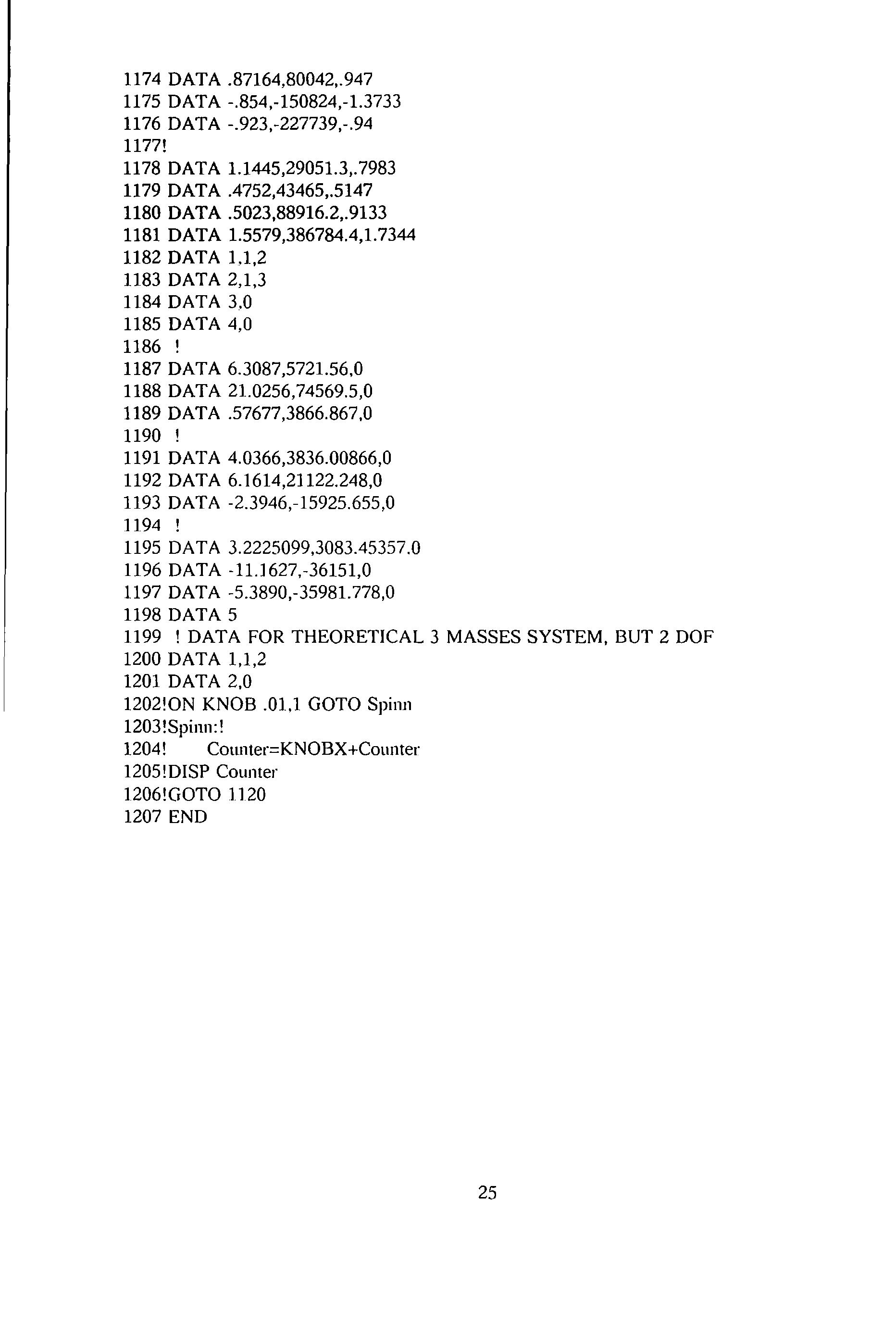
1199 ! DATA FOR THEORETICAL 3 MASSES SYSTEM, BUT 2 DOF
DATA 1,1,2 1201 DATA 2,0 1202!0N KNOB .01,1 GOTO Spim1
DATA 1,1,2 1183 DATA 2,1,3 1184 DATA 3.0 1185
1182
DATA
1186
1203!Spinn:! 1204!
1205! DISP Counter 1206!GOTO 1120 1207 END 25
1200
Counter=KNOBX+Counter
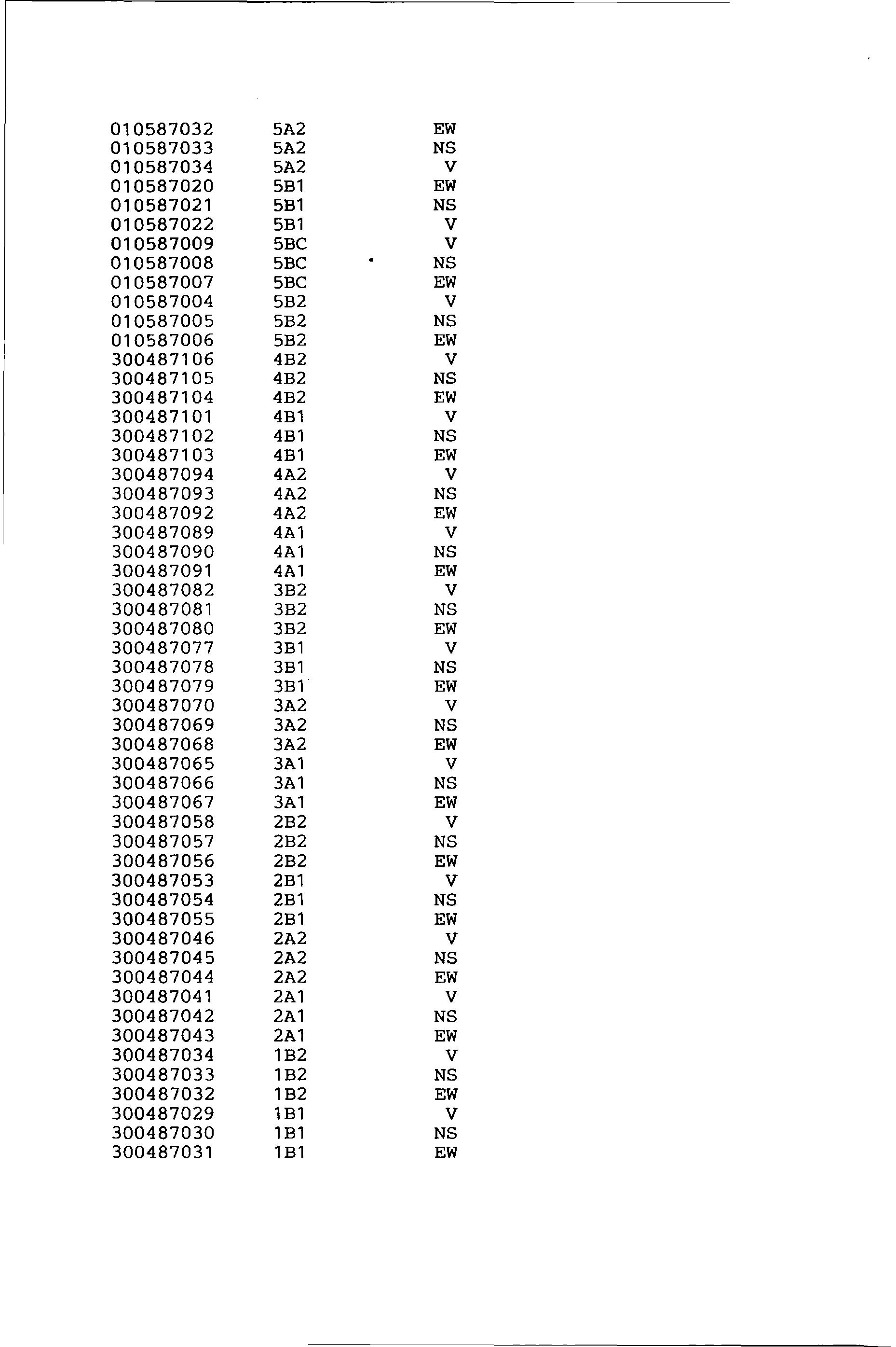
010587032 010587033 010587034 010587020 010587021 010587022 010587009 010587008 010587007 010587004 010587005 010587006 300487106 300487105 300487104 300487101 300487102 300487103 300487094 300487093 300487092 300487089 300487090 300487091 300487082 300487081 300487080 300487077 300487078 300487079 300487070 300487069 300487068 300487065 300487066 300487067 300487058 300487057 300487056 300487053 300487054 300487055 300487046 300487045 300487044 300487041 300487042 300487043 300487034 300487033 300487032 300487029 300487030 300487031 5A2 5A2 5A2 5B1 5B1 5B1 5BC 5BC 5BC 5B2 5B2 5B2 4B2 4B2 4B2 4B1 4B1 4B1 4A2 4A2 4A2 4A1 4A1 4A1 3B2 3B2 3B2 3B1 3B1 3B1 3A2 3A2 3A2 3A1 3A1 3A1 2B2 2B2 2B2 2B1 2B1 2B1 2A2 2A2 2A2 2A1 2A1 2A1 1B2 1B2 1 B2 1 B1 1 B1 1B1 EW NS V EW NS V V NS EW V NS EW V NS EW V NS EW V NS EW V NS EW V NS EW V NS EW V NS EW V NS EW V NS EW V NS EW V NS EW V NS EW V NS EW V NS EW
APPENDIX 8.3 A SCHEDULE OF TEST IDENTIFICATIONS
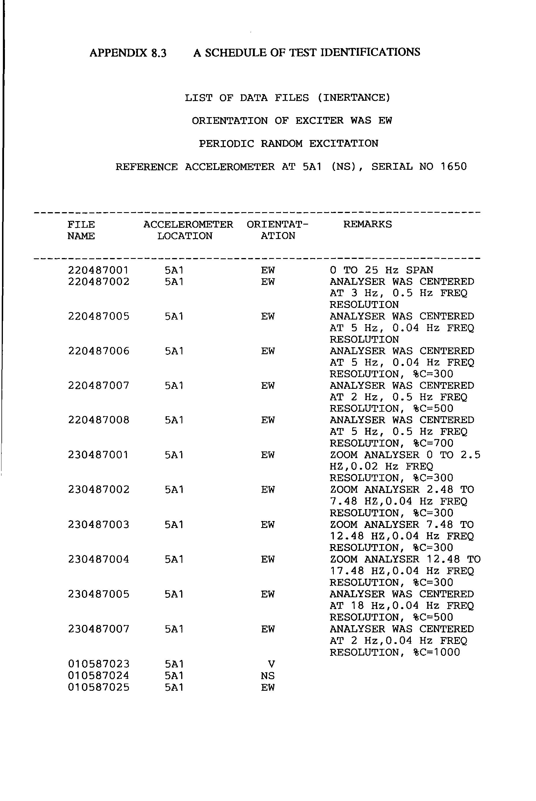
LIST OF DATA FILES (INERTANCE)
ORIENTATION OF EXCITER WAS EW
PERIODIC RANDOM EXCITATION
REFERENCE ACCELEROMETER AT 5A1 (NS), SERIAL NO 1650
FILE ACCELEROMETER ORIENTAT- REMARKS NAME LOCATION AT ION 220487001 5A1 EW 0 TO 25 Hz SPAN 220487002 5A1 EW ANALYSER WAS CENTERED AT 3 Hz, 0.5 Hz FREQ RESOLUTION 220487005 5A1 EW ANALYSER WAS CENTERED AT 5 Hz, 0.04 Hz FREQ RESOLUTION 220487006 5A1 EW ANALYSER WAS CENTERED AT 5 Hz, 0.04 Hz FREQ RESOLUTION, %C=300 220487007 5A1 EW ANALYSER WAS CENTERED AT 2 Hz, 0.5 Hz FREQ RESOLUTION, %C=500 220487008 5A1 EW ANALYSER WAS CENTERED AT 5 Hz, 0.5 Hz FREQ RESOLUTION, %C=700 230487001 5A1 EW ZOOM ANALYSER 0 TO 2.5 HZ,0.02 Hz FREQ RESOLUTION, %C=300 230487002 5A1 EW ZOOM ANALYSER 2.48 TO 7.48 HZ,0.04 Hz FREQ RESOLUTION, %C=300 230487003 5A1 EW ZOOM ANALYSER 7.48 TO 12.48 HZ,0.04 Hz FREQ RESOLUTION, %C=300 230487004 5A1 EW ZOOM ANALYSER 12.48 TO 17.48 HZ,0.04 Hz FREQ RESOLUTION, %C=300 230487005 5A1 EW ANALYSER WAS CENTERED AT 18 Hz,0.04 Hz FREQ RESOLUTION, %C=500 230487007 5A1 EW ANALYSER WAS CENTERED AT 2 Hz,0.04 Hz FREQ RESOLUTION, %C=1000 010587023 5A1 V 010587024 5A1 NS 010587025 5A1 EW
NOTE IN MOST OCCASSIONS, THE FOLLOWING CONDITIONS APPLY
A. SIGNAL FROM DARTEC LOAD CELL ON CHANNEL A OF SPECTRUM ANALYSER
B. SIGNAL FROM TRAVELLING ACCELEROMETER ON CHANNEL B OF SPECTRUM ANALYSER
EW WITH ACCELEROMETER SERIAL NUMBER 1652
NS WITH ACCELEROMETER SERIAL NUMBER 1653 (FOR FILES WITH DATE AND SERIAL NUMBER PRECEDE 300487008)
OR WITH ACCELEROMETER SERIAL NUMBER 1654 (FOR FILES WITH DATE AND SERIAL NUMBER AFTER 300487008)
V : WITH ACCELEROMETER SERIAL NUMBER 1658
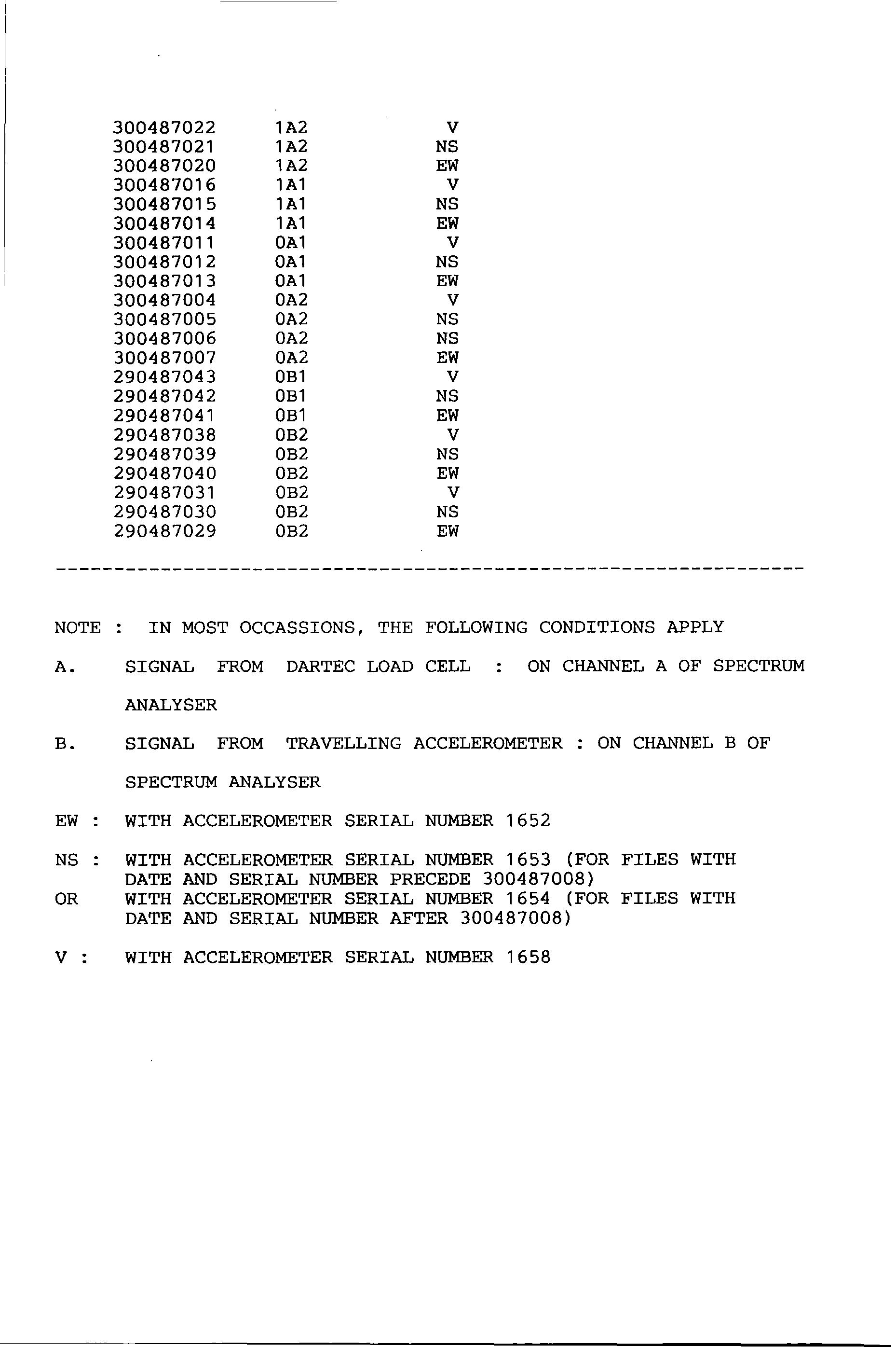
300487022 300487021 300487020 300487016 300487015 300487014 300487011 300487012 300487013 300487004 300487005 300487006 300487007 290487043 290487042 290487041 290487038 290487039 290487040 290487031 290487030 290487029 1A2 1A2 1A2 1A1 1 A1 1 A1 OA1 OA1 OA1 OA2 OA2 OA2 OA2 OB1 OB1 OB1 OB2 OB2 OB2 OB2 OB2 OB2 V NS EW V NS EW V NS EW V NS NS EW V NS EW V NS EW V NS EW
LIST OF DATA FILES (TRANSMISSIBILITY)
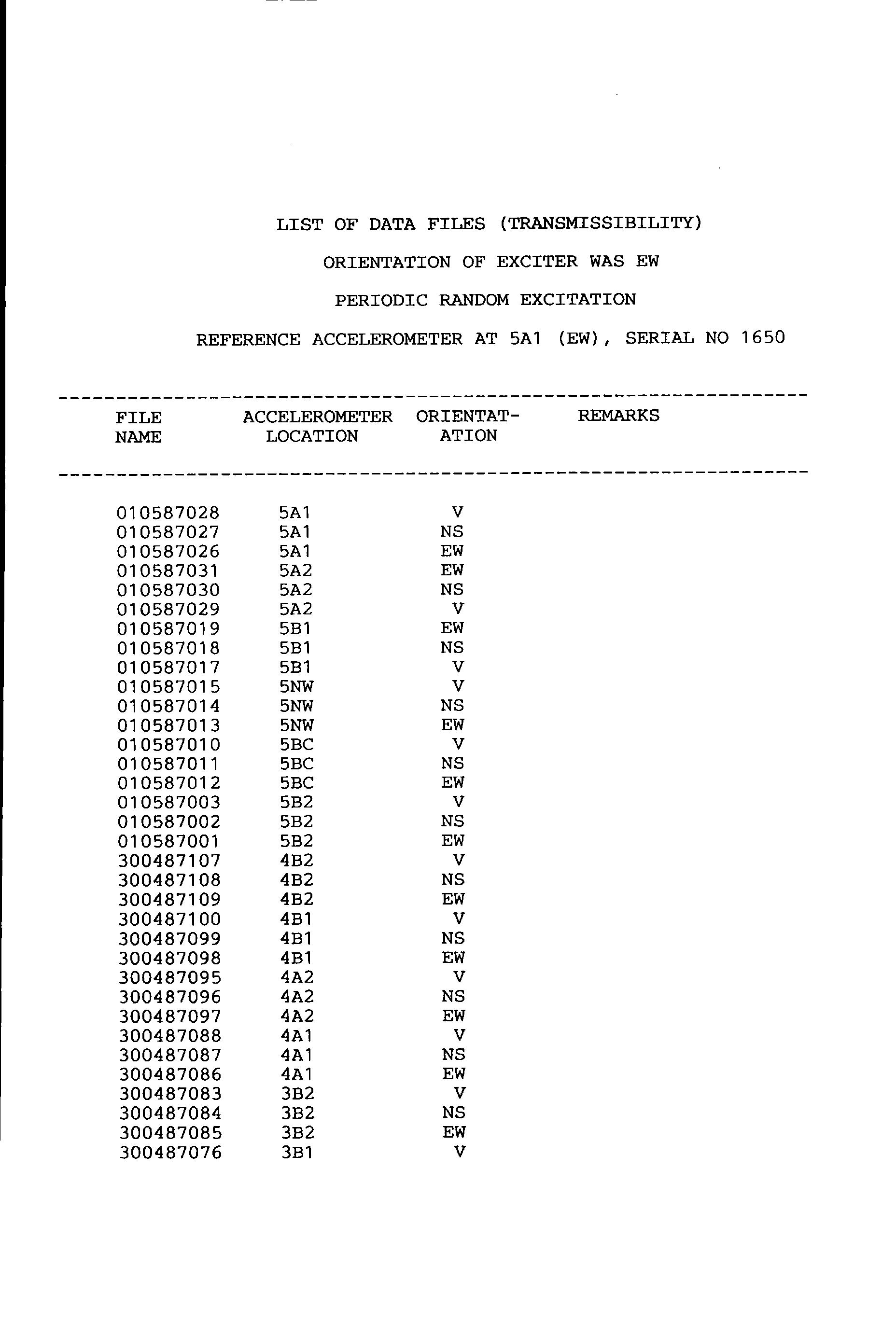
PERIODIC RANDOM EXCITATION
REFERENCE ACCELEROMETER AT 5A1 (EW), SERIAL NO 1650
ORIENTATION OF EXCITER WAS EW
----------------------------------------------------------------FILE NAME ACCELEROMETER ORIENTATLOCATION ATION REMARKS 010587028 5A1 V 010587027 5A1 NS 010587026 5A1 EW 010587031 5A2 EW 010587030 5A2 NS 010587029 5A2 V 010587019 5B1 EW 010587018 5B1 NS 010587017 5B1 V 010587015 5NW V 010587014 5NW NS 010587013 5NW EW 010587010 5BC V 010587011 5BC NS 010587012 5BC EW 010587003 5B2 V 010587002 5B2 NS 010587001 5B2 EW 300487107 4B2 V 300487108 4B2 NS 300487109 4B2 EW 300487100 4B1 V 300487099 4B1 NS 300487098 4B1 EW 300487095 4A2 V 300487096 4A2 NS 300487097 4A2 EW 300487088 4A1 V 300487087 4A 1 NS 300487086 4A1 EW 300487083 3B2 V 300487084 3B2 NS 300487085 3B2 EW 300487076 3B1 V
NOTE IN MOST OCCASSIONS, THE FOLLOWING CONDITIONS APPLY
A. SIGNAL FROM REFERENCE ACCELEROMETER ON CHANNEL A OF SPECTRUM ANALYSER
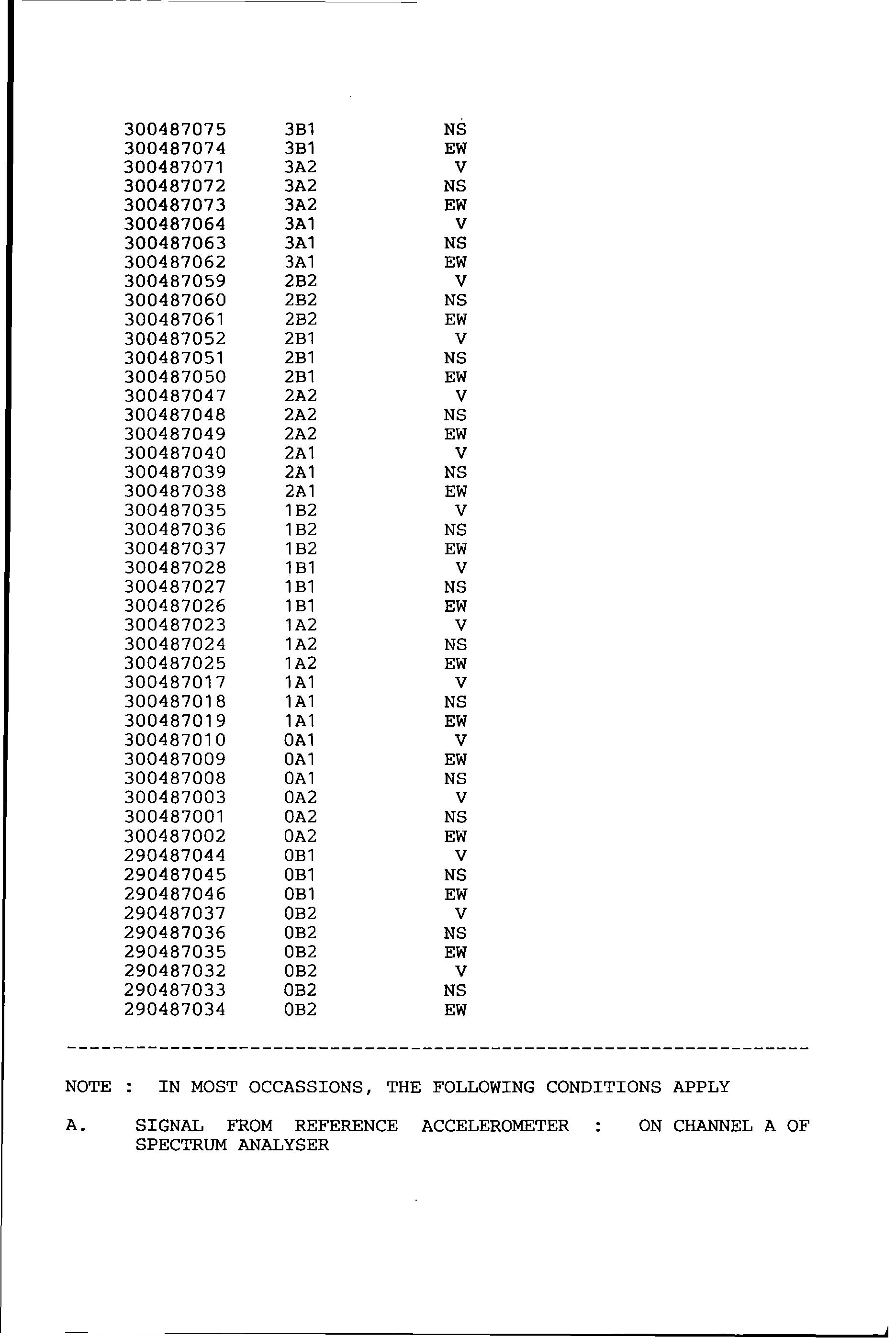
300487075 3B1 NS 300487074 3B1 EW 300487071 3A2 V 300487072 3A2 NS 300487073 3A2 EW 300487064 3A1 V 300487063 3A1 NS 300487062 3A1 EW 300487059 2B2 V 300487060 2B2 NS 300487061 2B2 EW 300487052 2B1 V 300487051 2B1 NS 300487050 2B1 EW 300487047 2A2 V 300487048 2A2 NS 300487049 2A2 EW 300487040 2A1 V 300487039 2A1 NS 300487038 2A1 EW 300487035 1 B2 V 300487036 1B2 NS 300487037 1B2 EW 300487028 1 B1 V 300487027 1 B1 NS 300487026 1 B1 EW 300487023 1A2 V 300487024 1A2 NS 300487025 1 A2 EW 300487017 1 A1 V 300487018 1 A1 NS 300487019 1 A1 EW 300487010 OA1 V 300487009 OA1 EW 300487008 OA1 NS 300487003 OA2 V 300487001 OA2 NS 300487002 0A2 EW 290487044 OB1 V 290487045 OB1 NS 290487046 OB1 EW 290487037 OB2 V 290487036 OB2 NS 290487035 OB2 EW 290487032 OB2 V 290487033 OB2 NS 290487034 OB2 EW -----------------------------------------------------------------
B. SIGNAL FROM TRAVELLING ACCELEROMETER SPECTRUM ANALYSER
EW WITH ACCELEROMETER SERIAL NUMBER 1652
ON CHANNEL B OF
NS WITH ACCELEROMETER SERIAL NUMBER 1653 (FOR FILES WITH DATE AND SERIAL NUMBER PRECEDE 300487008)
OR WITH ACCELEROMETER SERIAL NUMBER 1654 (FOR FILES WITH DATE AND SERIAL NUMBER AFTER 300487008)
V : WITH ACCELEROMETER SERIAL NUMBER 1658

LIST OF DATA FILES (INERTANCE)
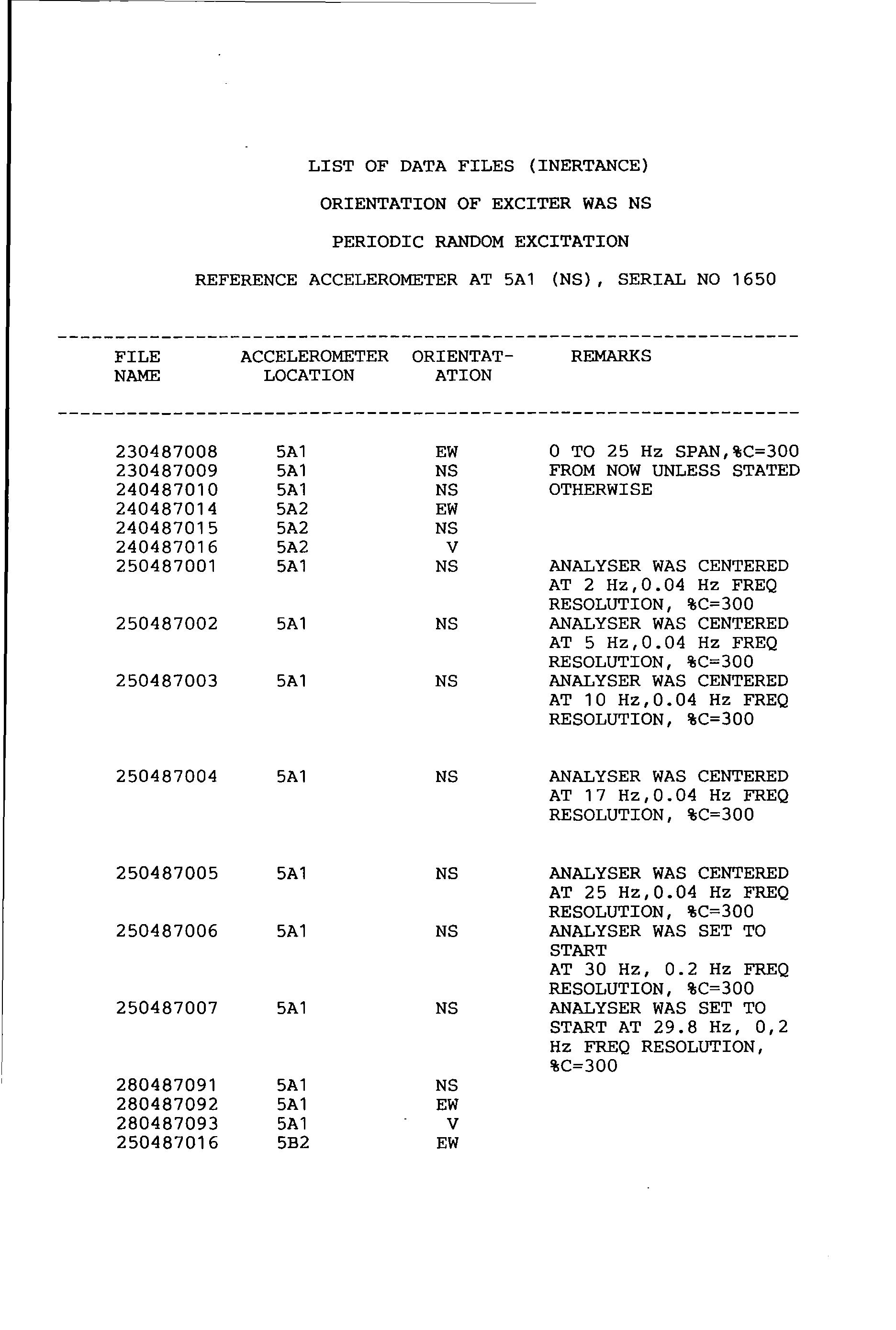
ORIENTATION OF EXCITER WAS NS
PERIODIC RANDOM EXCITATION
REFERENCE ACCELEROMETER AT 5A1 (NS), SERIAL NO 1650
FILE NAME ACCELEROMETER ORIENTATLOCATION ATION REMARKS ----------------------------------------------------------------230487008 5A1 EW 0 TO 25 Hz SPAN,%C=300 230487009 5A1 NS FROM NOW UNLESS STATED 240487010 5A1 NS OTHERWISE 240487014 5A2 EW 240487015 5A2 NS 240487016 5A2 V 250487001 5A1 NS ANALYSER WAS CENTERED AT 2 Hz,0.04 Hz FREQ RESOLUTION, %C=300 250487002 5A1 NS ANALYSER WAS CENTERED AT 5 Hz,0.04 Hz FREQ RESOLUTION, %C=300 250487003 5A1 NS ANALYSER WAS CENTERED AT 10 Hz,0.04 Hz FREQ RESOLUTION, %C=300 250487004 5A1 NS ANALYSER WAS CENTERED AT 17 Hz,0.04 Hz FREQ RESOLUTION, %C=300 250487005 5A1 NS ANALYSER WAS CENTERED AT 25 Hz,0.04 Hz FREQ RESOLUTION, %C=300 250487006 5A1 NS ANALYSER WAS SET TO START AT 30 Hz, 0.2 Hz FREQ RESOLUTION, %C=300 250487007 5A1 NS ANALYSER WAS SET TO START AT 29.8 Hz, 0,2 Hz FREQ RESOLUTION, %C=300 280487091 5A1 NS 280487092 5A1 EW 280487093 5A1 V 250487016 5B2 EW
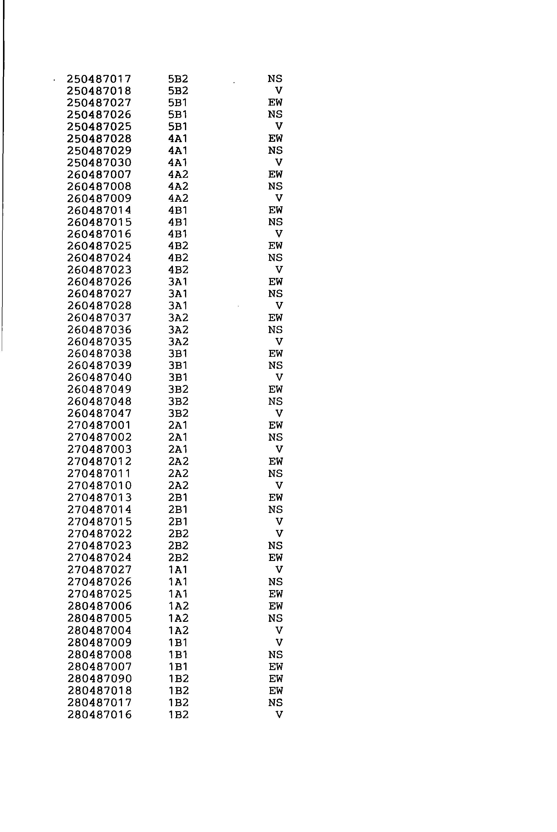
250487017 5B2 NS 250487018 5B2 V 250487027 5B1 EW 250487026 5B1 NS 250487025 5B1 V 250487028 4A1 EW 250487029 4A1 NS 250487030 4A1 V 260487007 4A2 EW 260487008 4A2 NS 260487009 4A2 V 260487014 4B1 EW 260487015 4B1 NS 260487016 4B1 V 260487025 4B2 EW 260487024 4B2 NS 260487023 4B2 V 260487026 3A1 EW 260487027 3A1 NS 260487028 3A1 V 260487037 3A2 EW 260487036 3A2 NS 260487035 3A2 V 260487038 3B1 EW 260487039 3B1 NS 260487040 3B1 V 260487049 3B2 EW 260487048 3B2 NS 260487047 3B2 V 270487001 2A1 EW 270487002 2A1 NS 270487003 2A1 V 270487012 2A2 EW 270487011 2A2 NS 270487010 2A2 V 270487013 2B1 EW 270487014 2B1 NS 270487015 2B1 V 270487022 2B2 V 270487023 2B2 NS 270487024 2B2 EW 270487027 1 A1 V 270487026 1 A1 NS 270487025 1 A1 EW 280487006 1A2 EW 280487005 1A2 NS 280487004 1A2 V 280487009 1 B1 V 280487008 1B1 NS 280487007 1B1 EW 280487090 1B2 EW 280487018 1B2 EW 280487017 1B2 NS 280487016 1B2 V
NOTE IN MOST OCCASSIONS, THE FOLLOWING CONDITIONS APPLY
A. SIGNAL FROM DARTEC LOAD CELL : ON CHANNEL A OF
B.
SPECTRUM ANALYSER
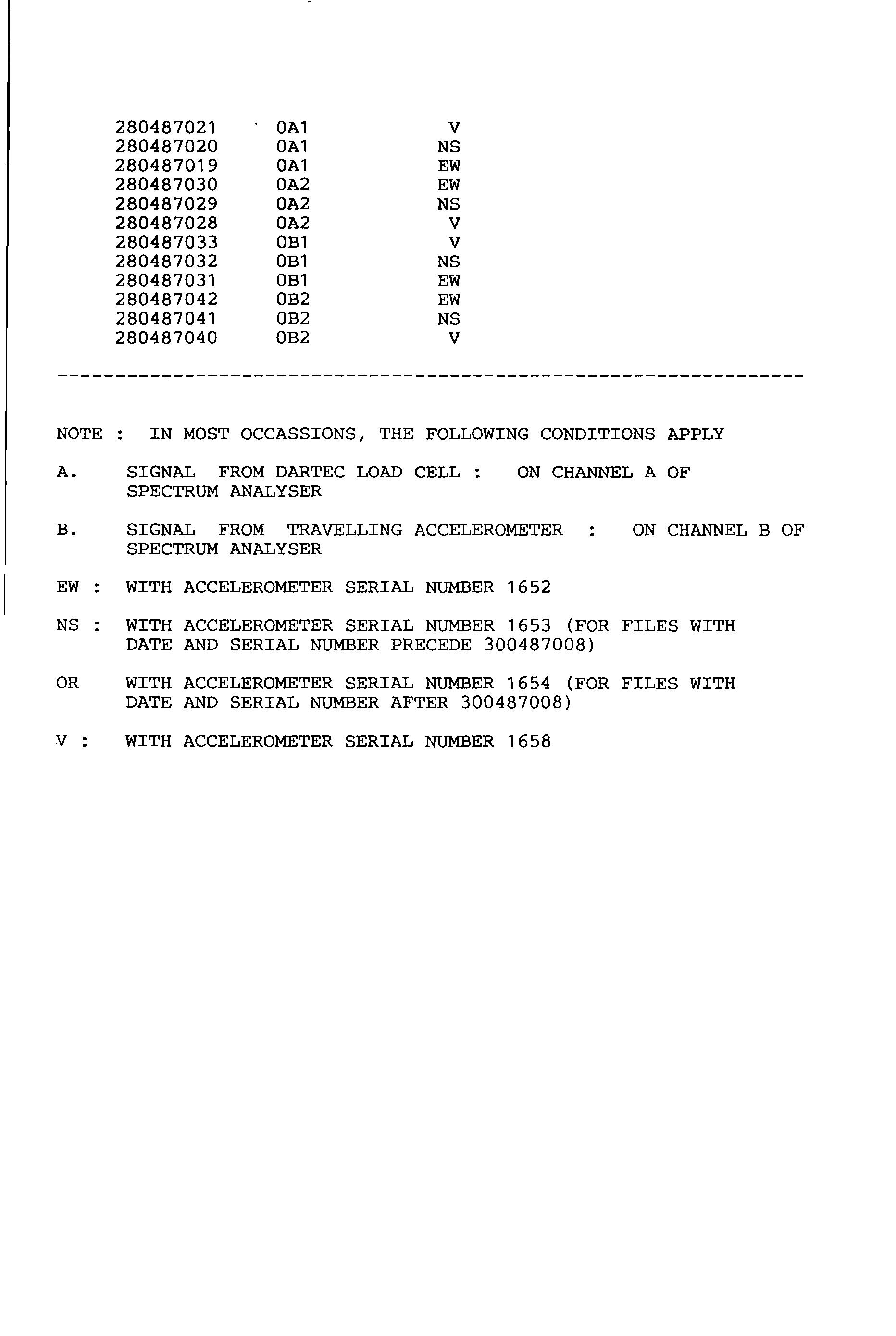
SIGNAL FROM TRAVELLING ACCELEROMETER SPECTRUM ANALYSER
EW WITH ACCELEROMETER SERIAL NUMBER 1652
ON CHANNEL B OF
NS WITH ACCELEROMETER SERIAL NUMBER 1653 (FOR FILES WITH DATE AND SERIAL NUMBER PRECEDE 300487008)
OR WITH ACCELEROMETER SERIAL NUMBER 1654 (FOR FILES WITH DATE AND SERIAL NUMBER AFTER 300487008)
V : WITH ACCELEROMETER SERIAL NUMBER 1658
280487021 280487020 280487019 280487030 280487029 280487028 280487033 280487032 280487031 280487042 280487041 280487040 OA1 OA1 OA1 OA2 OA2 OA2 OB1 OB1 OB1 OB2 OB2 OB2 V NS EW EW NS V V NS EW EW NS V
LIST OF DATA FILES (TRANSMISSIBILTY)
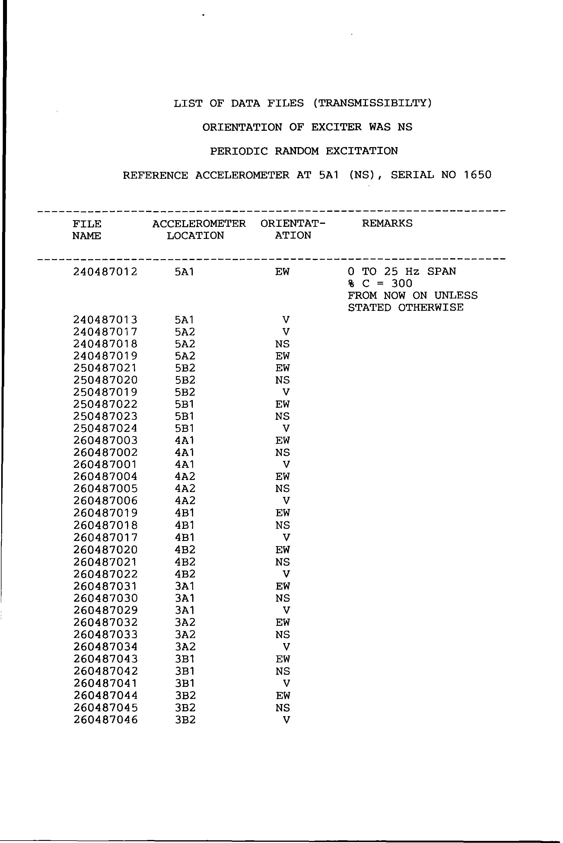
ORIENTATION OF
PERIODIC RANDOM EXCITATION REFERENCE
EXCITER
WAS NS
ACCELEROMETER AT 5A1 (NS), SERIAL
1650 FILE ACCELEROMETER ORIENT AT- REMARKS NAME LOCATION AT ION ----------------------------------------------------------------240487012 5A1 EW 0 TO 25 Hz SPAN % c = 300 FROM NOW ON UNLESS STATED OTHERWISE 240487013 5A1 V 240487017 5A2 V 240487018 5A2 NS 240487019 5A2 EW 250487021 5B2 EW 250487020 5B2 NS 250487019 5B2 V 250487022 5B1 EW 250487023 5B1 NS 250487024 5B1 V 260487003 4A1 EW 260487002 4A1 NS 260487001 4A1 V 260487004 4A2 EW 260487005 4A2 NS 260487006 4A2 V 260487019 4B1 EW 260487018 4B1 NS 260487017 4B1 V 260487020 4B2 EW 260487021 4B2 NS 260487022 4B2 V 260487031 3A1 EW 260487030 3A1 NS 260487029 3A1 V 260487032 3A2 EW 260487033 3A2 NS 260487034 3A2 V 260487043 3B1 EW 260487042 3B1 NS 260487041 3B1 V 260487044 3B2 EW 260487045 3B2 NS 260487046 3B2 V
NO
NOTE IN MOST OCCASSIONS, THE FOLLOWING CONDITIONS APPLY
A.
B.
SIGNAL FROM REFERENCE ACCELEROMETER SPECTRUM ANALYSER
SIGNAL FROM TRAVELLING ACCELEROMETER SPECTRUM ANALYSER
EW WITH ACCELEROMETER SERIAL NUMBER 1652
NS WITH ACCELEROMETER SERIAL NUMBER 1653 (FOR FILES WITH DATE AND SERIAL NUMBER PRECEDE 300487008)
OR WITH ACCELEROMETER SERIAL NUMBER 1654 (FOR FILES WITH DATE AND SERIAL NUMBER AFTER 300487008)
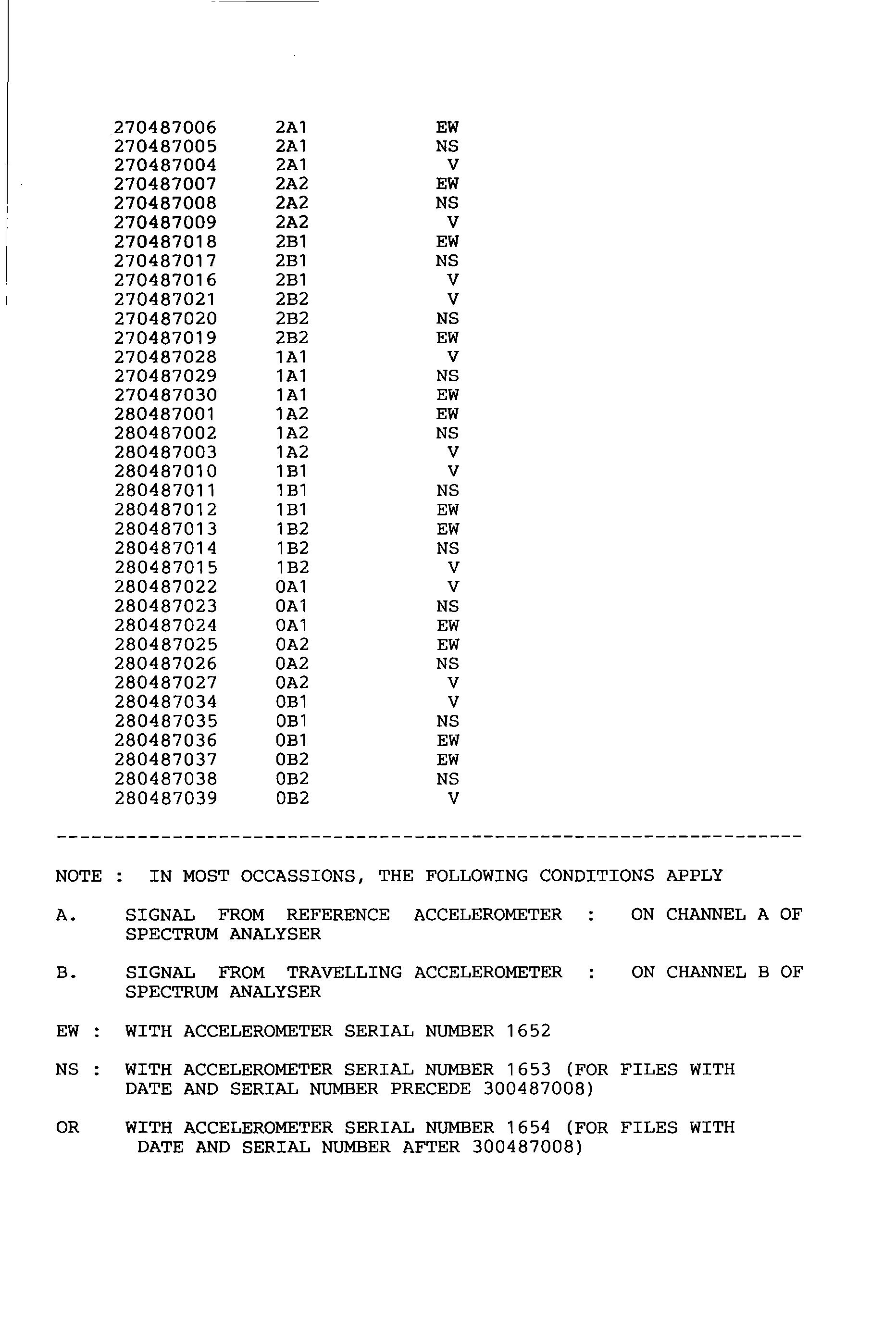
270487006 270487005 270487004 270487007 270487008 270487009 270487018 270487017 270487016 270487021 270487020 270487019 270487028 270487029 270487030 280487001 280487002 280487003 280487010 280487011 280487012 280487013 280487014 280487015 280487022 280487023 280487024 280487025 280487026 280487027 280487034 280487035 280487036 280487037 280487038 280487039 2A1 2A1 2A1 2A2 2A2 2A2 2B1 2B1 2B1 2B2 2B2 2B2 1 A1 1A1 1 A 1 1A2 1A2 1A2 1 B1 1 B1 1 B1 1B2 1 B2 1B2 OA1 0A1 OA1 OA2 OA2 OA2 0B1 OB1 OB1 0B2 OB2 OB2 EW NS V EW NS V EW NS V V NS EW V NS EW EW NS V V NS EW EW NS V V NS EW EW NS V V NS EW EW NS V
CHANNEL
OF
CHANNEL
ON
A
ON
B OF

·' , W·ITH ACCELER0METER ·SERillAL :Nl.<JMBER 1l)6 5f!, L \ I. - - •'
RESPONSE DECAY TESTS (TIME DATA)
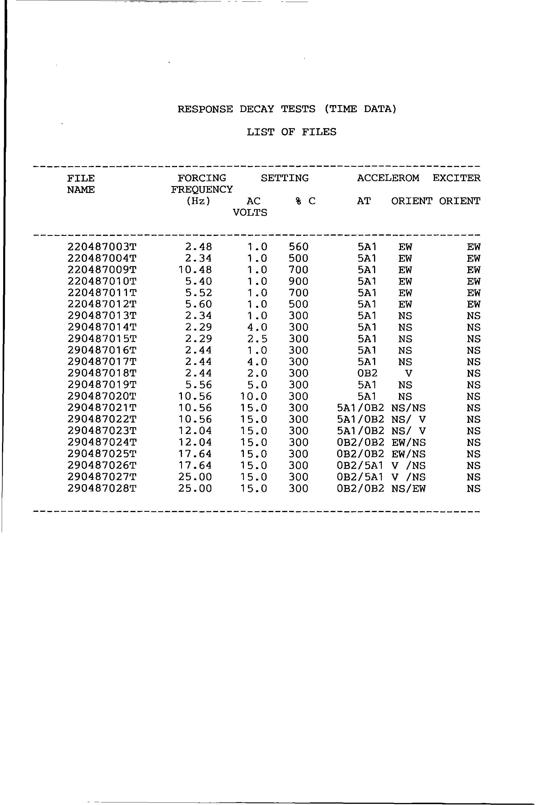
----------------------------------------------------------------FILE FORCING SETTING ACCELEROM EXCITER NAME FREQUENCY (Hz) AC % c AT ORIENT ORIENT VOLTS ----------------------------------------------------------------220487003T 2.48 1. 0 560 5A1 EW EW 220487004T 2.34 1 . 0 500 5A1 EW EW 220487009T 10.48 1 . 0 700 5A1 EW EW 220487010T 5.40 1.0 900 5A1 EW EW 220487011T 5.52 1 . 0 700 5A1 EW EW 220487012T 5.60 1.0 500 5A1 EW EW 290487013T 2.34 1.0 300 5A1 NS NS 290487014T 2.29 4.0 300 5A1 NS NS 290487015T 2.29 2.5 300 5A1 NS NS 290487016T 2.44 1 . 0 300 5A1 NS NS 290487017T 2.44 4.0 300 5A1 NS NS 290487018T 2.44 2.0 300 OB2 V NS 290487019T 5.56 5.0 300 5A1 NS NS 290487020T 10.56 10.0 300 5A1 NS NS 290487021T 10.56 1 5. 0 300 5A1/0B2 NS/NS NS 290487022T 10.56 1 5. 0 300 5A1/0B2 NS/ V NS 290487023T 12.04 1 5. 0 300 5A1/0B2 NS/ V NS 290487024T 12.04 1 5. 0 300 0B2/0B2 EW/NS NS 290487025T 17.64 1 5. 0 300 0B2/0B2 EW/NS NS 290487026T 17.64 1 5. 0 300 0B2/5A1 V /NS NS 290487027T 25.00 1 5. 0 300 0B2/5A1 V /NS NS 290487028T 25.00 1 5. 0 300 0B2/0B2 NS/EW NS -----------------------------------------------------------------
LIST OF FILES
LIST OF STEP-SINE TESTS DATA FILES

FILE FORCING SETTING ACCELEROM EXCITER NAME FREQUENCY (Hz) AC % c AT ORIENT ORIENT START STOP STEP VOLTS ----------------------------------------------------------------230487006S 2.0 2.8 . 1 3.0 1000 5A1 NS NS 230487010S 2.2 2.5 .02 1 . 5 300 5A1 NS NS 230487011S 2.2 2.4 .02 2.0 300 5A1 NS NS 240487001S 2.0 2.13 .01 1 • 5 300 5A1 NS NS 240487002S 2.0 2.34 .01 1 • 5 300 5A1 NS NS 240487003S 2.34 2.40 .01 1 . 5 300 5A1 NS NS 240487004S 2.40 2.47 .01 1 . 5 300 5A1 NS NS 240487005S 2.47 2.52 .01 1.5 300 5A1 NS NS 240487006S 2.0 2.40 . 01 3.0 300 5A1 NS NS 240487007S 2.40 2. 50 .01 3.0 300 5A1 NS NS 240487008S 2.30 2.40 .01 2.5 300 5A1 NS NS 240487009S 2.40 2.50 .01 2.5 300 5A1 NS NS 250487008S 2.40 2.50 .02 1 . 0 300 5A1 NS NS 250487009S 2.40 2.50 .02 1 . 66 300 5A1 NS NS 250487010S 2.40 2.50 .02 2.33 300 5A1 NS NS 250487011S 2.40 2.50 .02 2.50 300 5A1 NS NS 250487012S 2.40 2.50 .02 3.00 300 5A1 NS NS 250487013S 2.40 2.50 .02 3.50 300 5A1 NS NS 250487014S 2.40 2.50 .02 4.00 300 5A1 NS NS 250487015S 2.35 2.42 .02 4.00 300 5A1 NS NS 260487010S 2.0 300 4A2 EW NS 260487011S 2.5 300 4A2 EW NS 260487012S 3.0 300 4A2 EW NS 260487013S 3.5 300 5A1 EW NS 290487001S 2.28 2.38 .01 1 • 0 300 OB2 EW NS 290487002S 2.28 2.38 . 01 1 . 5 300 OB2 EW NS 290487003S 2.28 2.38 .01 2.0 300 OB2 EW NS 290487004S 2.25 2.30 . 01 2.5 300 5A1 NS NS 290487005S 2.25 2.30 . 01 3.0 300 5A1 N8 N8 2904870068 2.25 2.30 .01 4.0 300 5A1 N8 N8 2904870078 2.25 2.30 .01 4.5 300 5A1 N8 N8 2904870088 2.25 2.30 .01 2.0 300 5A1 N8 NS 290487009S 2.25 2.30 .01 2.0 300 5A1 N8 N8 2904870108 2.25 2.30 . 01 1 . 0 300 5A1 N8 N8 290487011S 2.25 2.30 .01 10.0 300 5A1 N8 N8 290487012S 2.25 2.30 .01 10.0 300 5A1 N8 N8 0105870358 10.00 12.00 1.0 300 5A1 V NS
REFERENCES
1.1 Williams C. 'The real perfonnance of some civil engineering structures.' PhD thesis, Plymouth Polytechnic, 1979.
1.2 British Standard Code of Practice, CP 3, Chapter V: Part 2: Code of basic data for the design of buildings, BSI, London, 1972.
1.3 Oppenheim I J. 'The effects of cladding on tall buildings.' PhD thesis, Cambridge University, UK, 1972.
1.4 Palsson H. 'Influence of non-structural cladding on dynamic properties and perfomtance of high rise building.' PhD thesis, Georgia Institute ofTechnology, USA, 1982.
1.5 Freeman SA. 'Racking tests of high-rise building partitions.' Journal of the Structural Division of ASCE, ST8, August 1977, Paper 13136.
1.6 Honda K K. 'Measurements and evaluation of building response to ground motion at various stages of construction.' ASCE-EMD Speciality Conference on Dynamic Response of Structures; Instrumentation, Test Methods and System Identification, University of California, Los Angeles, March 1976.
1.7 Blume J A, Binder R W. 'Periods of a modem multi-storey office building during construction'. Proceedings of the Second World Conference on Earthquake Engineering. Tokyo, Japan, 1960.
1.8 Mirtaheri M. 'Assessment of lateral and torsional stiffness characteristics of medium-rise buildings.' PhD thesis, Virginia Polytechnic and State University, USA, 1983.
2.1 Hudson DE, Keightley W 0 and Nielsen N N. 'A new method for the measurement of the natural periods of buildings.' Bulletin of the Seismological Society of America, VS4(1), pp 233-241, February 1964.
2.2 Czamecki R M. 'Dynamic testing of buildings using man induced vibration.' Journal of Sound and Vibration, October 1974.
2.4 Ward H S and Crawford R. 'Wind induced vibrations and building modes.' Bulletin of the Seismological Society of America, V 56, pp 421 - 436, August 1966.
2.5 Trifunac M D. 'Ambient vibration tests of a 39 storey steel frame building.' Pasadena, Earthquake Engineering Research Laboratory, California Institute of Technology, University of California at Berkeley Catalogue Reference (UCB EERC 545.2 T72 1970) No 70 - 02, 1970.
2.6 Lam L CH and Lam RP. 'Observation on some salient features offull-scale dynamic wind forces on a multi-storey building.' Proceedings of the Institution of Civil Engineers, Pt 2, December 1973.
2.7 Dalgliesh W A And Rainer J H. 'Measure of wind induced displacements and accelerations of a 57 storey building in Toronto.' National Research Council of Canada, Division of Building Research, April 1978.
2.9 Hudson D E et al. 'Response of structure to an explosive-generated ground shock.' Pasadena, Earthquake Engineering Research Laboratory, California Institute of Technology, University of California at Berkeley, Catalogue Reference (UCB EERC 545.1 H83) 1952.
2.1 0 Housner G W. 'Behaviour of structure during earthquakes.' Journal of Engineering Mechanics Division, ASCE, Vol 85, EM 4, Paper 2220, October 1959.

2.11
Jennings PC. 'Response of simple yielding structures to earthquake excitation.' Pasadena, Earthquake Engineering Research Laboratory, California Institute of Technology, University of California at Berkeley, Catalogue Reference (UCB EERC 530 J37 1963), 1963.
2.12 Jennings PC and Husid R. 'Collapse of yielding structures during earthquakes.' Journal of the Engineering Mechanics Division, Proceedings of ASCE, EM 5, Paper 6154, pp I045 -I 065, V94(5), October 1968.
2.13 Hiroyoshi and Kobayashi. 'Dynamic properties of building decided by measurement of vibration during earthquake.' Proceedings of the Second World Conference on Earthquake Engineering, Tokyo and Kyoto, Japan, July 11 - 18 1960. (UCB EERC 500 M395 E- 22).
2.14
Hudson D E. 'A new vibration exciter for dynamic test of full scale structure.' Pasadena, Earthquake Engineering Research Laboratory, California Institute of Technology, University of California at Berkeley, 1961.
2.15 Takeuchi M. 'Vibration characteristics of buildings: Part 1, vibration characteristics of actual building determined by vibration tests.' Proceedings of the Second World Conference on Earthquake Engineering, Tokyo and Kyoto, Japan, July 11 - 18 1960. Vol 2, pp 961 - 982, 1960. (UCB EERC 500 M395 E - 22).
2.16 Burroughs H L, Kinlock H and Winney P E. 'Vibration studies on full scale structures. Proceedings of the SECED Conference on Dynamic Waves in Civil Engineering. University College, Swansea, July 1970.
2.17 Stephen RH, Hollings J P and Bouwkamp J G. 'Dynamic behaviour of a multi-storey pyramid-shaped building.' Earthquake Engineering Research Centre Report, University of California at Berkeley, Springfield, Virginia. (UCB EERC 545.1 S73 1974). Report No 73- 17, 1973.

2.18 Galambos TV and Mayes R C. 'Lessons from dynamic tests of an eleven storey building.' Journal of Engineering Structures, VI, October 1979.
2.19 Omori F. 'Note on applied seismology.' Bereich der I Intern Seismologischen Konferenz, 355, 1901.
2.20 US Coast and Geodetic Survey. 'Earthquake investigation in California, 1934- 1935.' Special Publication No 201, 1936, USA.
2.21 Hudson D E. 'A new vibration exciter for dynamic tests of full scale structures. Pasadena, Earthquake Engineering Research Laboratory, California Institute of Technology, University of California at Berkeley, Catalogue Reference (UCB EERC 545.1 H38 1961), September 1961.
2.22 Karapetian B K. 'A study of vibrations of structures in nature.' Proceedings of the Third World Conference on Earthquake Engineering, Auckland, New Zealand, 22 January- I February 1965. Organised by the New Zealand National Committee on Earthquake (UCB EERC 400 W66 1965).
2.23 Hudson DE. 'Dynamic testing of buildings and special structures.' Experimental Techniques in Shock and Vibration, American Society of Mechanical Engineers 81- 91, 1962.
2.24 Jeary A P. 'The dynamic behaviour of tall buildings.' PhD thesis, University College London, UK, 1981.
2.25
Hudson DE. 'Resonance testing of full scale structures.' Journal of the Engineering Mechanics Division, Proceedings of the ASCE, New York, EM3 Paper No 3923, V90(3), pp I - 2, June 1964.
2.26 Keightley W 0, Housner G Wand Hudson DE. 'Vibration tests of the Encino Dam intake tower.' Pasadena, Earthquake Engineering Research Laboratory, California Institute of Technology, University of California at Berkeley, Catalogue Reference (UCB EERC 545.1 K37 1961), Report No 61 -75, 1961.
2.27 Keightley W 0. 'Vibration tests of structures.' Pasadena, Earthquake Engineering Research Laboratory, California Institute of Technology, University of California at Berkeley, Catalogue Reference (UCB EERC 545.1 KJ7 1963), 1963.
2.28 Nielsen N N. 'Dynamic response of multi-storey buildings.' PhD thesis, Pasadena, California Institute of Technology, University of California at Berkeley, (UCB EERC 525N53 1964),ReportNo64-60 1964.
2.29 Bouwkamp J G and Blohm J K. 'Dynamic response of two-storey steel frame structure.' Bulletin of the Seismological Society of America, V56, pp 1289- I 304, 1966.
2.30 Kuriowa J H. 'Vibration tests of a multi-storey building.' Pasadena, Earthquake Engineering Research Laboratory, California Institute of Technology, University of California at Berkeley, Catalogue Reference (UCB EERC 545.1 K86 1967), Report No 67- 66, 1967.
2.31 Jennings PC, Matthiesen R B and Hoerner J B. 'Forced vibrations of a 22-storey steel frame building.' Pasadena, Earthquake Engineering Research Laboratory, California Institute of Technology, University of California at Berkeley, Catalogue Reference (UCB EERC 545.1 JJ7 1971), Report No 71-01, February 1971.

2.32 Jennings PC and Kuriowa J H. 'Vibration and soil-structure interaction tests of a nine-storey reinforced concrete building.' Journal of the Engineering Mechanics Division, Proceedings of the ASCE, New York, V58(3), pp 891 -916, June 1968.
2.33 Clough R W, Chang KT et al. 'Dynamic response behaviour ofQuan Shui Dam.' University of California at Berkeley, Springfield, Virginia (UCB EERC 540 C593 1984Q), Report No UCB/EERC - 84/02.
2.34 Hall J F and Duron Z. 'Experimental and finite element studies of the forced vibration response of Morrow Point Dam.' Chichester, New York, J Wiley, 1988. Also Earthquake Engineering and Structural Dynamics Vl6 No 7, October 1988.
2.35 Jeary A P and Winney PE. 'Determination of structural damping of a large flue chimney from the response to wind excitation.' Proceedings of the Institution of Civil Engineers, Part 2, December 1972, 53, pp 569 - 577.
2.36 Jeary A P. 'Damping measurements from the dynamic behaviour of several large flue chimneys.' Proceedings of the Institution of Civil Engineers, Part 2, June 1974, 57, pp 321- 329.
2.37 Severn R T, Jeary A Pet al. 'Prototype dynamic studies on a rock fill dam and abuttress dam.' Proceedings of the !COLD XIII Congress Q15, R16, New Delhi, 1979.
2.38 Severn R T, Jeary A P and Ell is B R. 'Forced vibration tests and theoretical studies on dams.' Proceedings of the Institution of Civil Engineers, Part 2 , 1980.
2.39 Jeary, A P and Sparks PR. 'Some observation on the dynamic sway characteristics of concrete structures.' ACI Symposium on Vibrations of Concrete Structures, New Orleans, October 1977. Also Building Research Establishment (BRE}, Watford, England, Current Paper No 7/78. (UCB EERC 500 G7CP 7.78.)

2.40 Kawasumi K and Kanai K. 'Small amplitude vibrations of actual buildings. Proceedings of the First World Conference on Earthquake Engineering, Berkeley, California, Earthquake Engineering Research Institute (EERI}, Paper No 7( I}, 1956.
2.41 Hisada T and Kakagawa K. 'Vibration tests on various types of buildings up to failure.' Proceedings of the First World Conference on Earthquake Engineering, Berkeley, California, Earthquake Engineering Research Institute (EERI), Paper No 7( 11 ), 1956.
2.42 Englekirk RE and Matthiesen R B. 'Forced vibration of an eight storey reinforced concrete building.' Bulletin of the Seismological Society of America V57, pp 421 - 436, June 1967. Also University of California, Los Angeles, Report No 66 - 8, 1966, (UCB EERC 545.1 E542 1966).
2.43 Blume J A and Binder R W. 'Periods of a modem multi-storey office building during construction.' Proceedings of the Second World Conference on Earthquake Engineering, Tokyo, Japan, 11 - 18 July 1960. (UCB EERC 500 M395 E- 22).
2.44 Honda K K. 'Measurement and evaluation of high-rise building response to ground motion generated by underground nuclear detonation.' ASCE- EMD Speciality Conference on Dynamic Response of Structures: Instrumentation, Test Methods and System Identification, University of California, Los Angeles, march 1976.
2.45 Palsson H. 'Influence of non-structural cladding on dynamic properties and performance of high rise building.' PhD thesis, Georgia Institute of Technology, 1982.
2.46 Huang S CS. 'Measurement and interpretation of full scale building responses.' PhD thesis, University of California, Los Angeles, 1983.
2.47 Oppenheim I J. 'High rise building vibration properties an unexpected behaviour mechanism.' Proceedings of the North American Masonry Conference, August 1978, University of Colorado.
2.48 ESDU. 'Undamped natural vibration of core buildings.' Item No 81036, Engineering Science Data Unit (ESDU}, London, 1981.
2.49 ESDU. 'Undamped natural vibration of sway frame buildings and frame structures.' Item No 82019, Engineering Science Data Unit (ESDU}, London, 1982.
2.50 ESDU. 'Undamped natural vibration of shear buildings.' Item No 79005, Engineering Science Data Unit (ESDU}, London, 1979.
2.51 Taniguchi T. 'General principles of aseismic construction.' Iwanana Shoten, 61, Tokyo, 1934.
2.52 El lis BR. 'An assessment of the accuracy of predicting the fundamental natural frequencies of buildings and the implications concerning dynamic analysis of structures.' Proceedings of the Institution of Civil Engineers, part 2, 1980, 69, September, 763 - 776.
2.53 SEAOC. 'Recommended lateral force requirements and commentary.' Seismology Committee, Structural Engineers Association of California (SEAOC}, San Francisco, 1960, revised 1974 and 1980.
2.54 'Seismic provisions of state and local building codes and their enforcement.' National Conference of States on Building Codes and Standards, Building and Fire Research Laboratory, National Institute of Standards and Technology (US) 1992, (UCB EERC 610 N335 GCR 91599).
2.55 'Uniform Building Codes.' International Conference of Building Officials, Pasadena, 1961. Also 'Analysis of revisions to the Uniform Building Codes 1967 edition'. Pasadena, University of California, Los Angeles, Law Lib TIN84, C7606, b86a, 1976.
2.56 ESDU 'Damping of structures Part I: tall buildings.' Item No 83009, Engineering Science Data Unit (ESDU), London, 1983.
2.57 Blume J A. 'Response of high-rise building to ground motion tTom underground nuclear detonation.' Bulletin of the Seismological Society of America, V59, No 6, December 1969.
3.1
3.3
Love A EH. 'A treatise on the mathematical theory of elasticity.' Fourth Edition, Dover Publication, New York, ISBN 0486-60174-9, 1944.
Clark S K. 'Dynamics of continuous elements.' Prentice-Hall Inc New Jersey, 1972.
3.4 Richards T H. 'Energy methods in stress analysis with an introduction to finite element techniques.' Chichester: Horwood, new York, Halsted Press, Ellis Horwood Ltd, 1977.
3.5 Brebbia C A. 'The boundary element method for engineers.' First published in 1978 by Pentech Press Ltd.
3.6 Robinson J. 'Understanding Finite Element Stress Analysis.' Robinson and Associates, England, 1988.
3.7 Zienkiewica 0 C. 'The Finite Element Method in Engineering Science.' McGraw-Hill Publishing Company Ltd, London, 1971.
3.8 Richardson M H. Keynote address to the Second International Modal Analysis Conference, Orlando, Florida, 1984. Published by the Union College and the Society of Experimental Mechanics, New York, USA.
3.9 Bekey G A. 'System identification- an introduction and a survey.' Simulation, October, pp 15 1 - 166, 1970.
3.10 Young JP and On F J. 'Mathematical modelling via direct use of vibration data.' Society of Automotive Engineers paper 690615, October 1969.
3.11
Flannelly W G, McGarvey J Hand Berman A. 'A theory of identification of the parameters in the equation of motion of a structure through dynamic testing.' Paper No C-1, Symposium on Structural Dynamics, Loughborough University of Technology, March 1970.
3.12
Raney JP. 'Identification of complex structures using near resonance testing.' Shock and Vibration Bulletin, Vci138, Pt 2, 23- 32, USA, 1968.
3.13 Bishop RED and Gladwell GM L. 'An investigation into the theory of resonance testing.' Proceedings of the Royal Society Phil Trans 255 (A) 241, 1963.
3.14 Ewins DJ. 'Measurement and Application of Mechanical Mobility Data.' Published by Solartron Electronic Group Ltd, 1982.
3.15
Proceedings of the First to the Eleventh International Modal Analysis Conferences from 1981 to 1992. Published by the Union College and the Society of Experimental Mechanics, New York, USA.

3.16
Proceedings of the First to the Thirteenth International Seminar on Modal Analysis from 1976 - 1988. Published by the Katholieke Universiteit, Leuven, Belgium.
3.17 The International Journal of Analytical and Experimental Modal Analysis. Published quarterly by the Society of Experimental Mechanics (SEM) since 1988.
3.18 Mechanical Systems and Signal Processing. The journal published quarterly by the Academic Press, UK, since 1988.
3.19 lbanez P. 'Identification of dynamic structural models from experimental data.' PhD thesis, University of California, Los Angeles, March 1972.
3.20 Berman A and Flanelly W G. 'The theory of incomplete models of dynamic substructures.' AlAA/ASME Eleventh Structures and Structural Dynamics and Materials Conference, Denver, USA, 1970.
4.1 Dartec. 'Operation manual for the Dartec 5 kN Servo-Hydraulic Actuator'. Dartec Ltd, Stourbridge, West Midlands, 1984.
4.2 Tsand W F. 'Performance and calibration tests of the new linearly motion inertial exciter for full scale forced vibration tests.' Internal Report, Department of Civil Engineering, Plymouth Polytechnic, 1987.
4.3 Schaevitz. 'Linear and angular servo accelerometers.' Technical Bulletin 450 ID, Schaevita Engineering, Pennsauken, New Jersey, USA.
4.4 Racal. 'Operation manual for FM tape recorder.' Racal Therm ionic Ltd, Hythe, Southampton.
4.5 Philips. 'L F synthesiser I mHz- 2 mHz PM 5190 lnstruction Manual.' Phi lips, Pye Uniam Ltd, Cambridge, 1983.
4.6 Hewlett Packard. 'Instruction Manual HP3582A Real Time Spectrum Analyser.' Hewlett Packard, Altringham, Cheshire.
4.7 Hewlett Packard. 'Signal averaging with the HP3582A Spectrum Analyser.' Application note 245 - I, Hewlett Packard, Altringham, Cheshire.
4.8 Hewlett Packard. 'Accessing the 3582A memory with HP-lB.' Application note 245- 4, Hewlett Packard, Altringham, Cheshire.
5.1 Schiff A J. 'Identification of large structures using data from ambient and low level excitation.' A paper presented at the 1972 Winter Annual Meeting on 'System identification of vibrating structures: Mathematical models from test data', of the ASME.
5.2 Spitznogle F Rand Quazi. A H 'Representation and analysis of Time-limited signals using a complex exponential algorithm.' Journal of the Acoustical Society of America, Vol47, No 5 (part 1), May 1970.
5.3 Leonard F. 'ZMODAL. 'A new Modal identification technique.' The International Journal of Analytical and Experimental Modal Analysis, Vol3, No 2, Aprill988.
5.4 Tang Z Q and Qiu Y. 'Modal analysis using the time series analysis method (AR or ARMA MODEL) and its computer program design.' Proceedings of the second International Modal Analysis Conference, Orlando, USA, 1984, pp 559- 565. Published by Union College and the Society of Experimental Mechanics, New York, USA.

5.5
Void Hand Rocklin G. 'The numerical implementation of a multi-input modal estimation method for mini-computers.' Proceedings of the First International Modal Analysis Conference, Florida, 1982. Published by the Union College and the Society of Experimental Mechanics, New York, USA.
5.6 Pappa R Sand lbrahim SR. 'A Parametric study of the lbrahim Time Domain Modal Identification algorithm.' Shock and Vibration Bulletin, 5 1(3), 1981.
5. 7 Cooper J E. 'Comparison of some time-domain system identification techniques using approximate data correlations. The International Journal of Analytical and Experimental Modal Analysis, Vol4, No 2, April 1989.
5.8 Fullekrug U. 'Survey of parameter estimation methods in experimental modal analysis.' Proceedings of the Fifth International Modal Analysis Conference, London, 1987. Published by the Union College and the Society of Experimental Mechanics, New York, USA.
5.9 Kennedy CC and Pancu CD P. 'Use of vectors in vibration measurement and analysis.' Journal of Aero Sci 14 (11), 1947.
5.10 Ewins D and Gleeson PT. 'A method for modal identification of lightly damped structures.' Journal of Sound and Vibration 84(1), 57- 59, 1982.
5.11 Goyder H G D. 'Foolproof methods for frequency response measurements.' Proceedings of the Second International Conference on Recent Advances in Structural Dynamics, ISVR, University of Southampton, 1984.
5.12 Dobson B. 'A straight-line technique for extracting modal properties from frequency response.' Mechanical Systems and Signal Processing (1987) 1(1), 29- 40.
5.13 Ewins DJ. 'Modal testing: Theory and Practice'. Research Studies Press, Letchworth, Hertfordshire, England, 1984, ISBN 047190472.
5.14 Van Loon P. 'Modal parameters of mechanical structures.' PhD Dissertation, Katholieke Universiteit, Leuven, Belgium 1974.
5.15 Ewins DJ and Gleeson PT. 'A method for modal identification of lightly damped structures.' Journal of Sound and Vibration, V84( I), 1982.
5.16 Richardson M and Forrnenti D L. 'Parameter estimation from frequency response measurements using rational fraction polynomial.' Proceedings of the First International Modal Analysis Conference, Florida, 1982. Published by the Union College and the Society of Experimental Mechanics, New York, USA.
5.17 Richard son M and Forrnenti D L. 'Global curve-fitting of frequency response measurements using the rational fraction polynomial method.' Proceedings of the Third International Modal Analysis Conference, Florida, 1985. Published by the Union College and the Society of Experimental Mechanics, New York, USA.

5.18 Maia N M and Ewins D J. 'A new approach for the modal identification of lightly damped structures.' Mechanical Systems and Signal Processing, Vol3 No 2, April 1989.
5.19 Metwalli S M. 'State-Space approach to Modal analysis.' Proceedings of the Third International Modal Analysis Conference, Florida, 1985. Published by the Union College and the Society of Experimental Mechanics, New York, USA.
5.20 Zhang L, Kanda H, Brown D Land Allemang R J. 'A Poly-reference frequency domain method for modal parameter identification.' ASME Paper No 85-DET-1 06, 1985.
6.1 Gleeson PT. 'Identification of spatial models.' PhD thesis, Department of Mechanical Engineering, Imperial College, University of London, 1979.
6.2 Rodden W P. 'A method for deriving structural influence coefficients from ground vibration tests.' Journal of AIAA, Vol5 No 5, May 1967, pp 991- 1000.
6.3 Raney J P and Hewlett J T. 'Identification of structural systems by the use of near-resonance testing.' NASA Technical Note NASA-TN-D-5069,1969.
6.4 Ross R G. 'Synthesis of stiffness and mass matrices.' Society of Automotive Engineers Paper No 710787, Annual Society of Automotive Engineers Meeting, Los Angeles, 1971.
6.5 Thoren A R. 'Derivation of mass and stiffuess matrices from dynamic test data.' AIAA paper 72- 346, Thirteenth Structures, Structural Dynamics and Materials Conference, San Antonio, Texas, 12 April 1972.
6.6 Young P and On F J. 'Mathematical modelling via direct use of vibration data.' Society of Automotive Engineers Paper 690615, Society of Automotive Engineers, 1969.
6.7 Kozin F and Kozin CH. 'Identification of linear systems. Final Report on simulation studies.' Reports submitted to NASA under Contract No NAS 5 -I 0 I 06, 1968.
6.8 Nielsen N N. 'Dynamic response of multi-storey buildings.' PhD thesis, California Institute of Technology, June 1964.
6.9 Sokal Y J. 'Identification of static properties of building structures from small amplitude resonance testing.; Shock and Vibration Conference, Monash University, Melbourne, 1974.
6.10 Potter Rand Richardson M. 'Mass, stiffness and damping matrices from measured modal parameters.' ISA International Instrumentation Symposium-Automat Conference, New York, 28 - 31 October 1974.
6.11
O'Callahan J C et al. 'Development of mass and stiffness matrices for an analytical model using experimental modal data.' Proceedings of the Second International Modal Analysis Conference, Orlando, Florida, February 1984. Published by the Union College and the Society of Experimental Mechanics, New York, USA.

6.12 O'Callahan J C and Leung R K. 'Optimisation of mass and stiffness matrices using a generalised inverse technique on the measured modes.' Proceedings of the Third International Modal Analysis Conference, Orlando, Florida, February 1985. Published by the Union College and the Society of Experimental Mechanics, New York, USA.
6.13 Baruch M. 'Optimal correction of mass and stiffness matrices using measured modes.' AIAA Journal, Vo120, November 1982.
6.14 Tsang W F and Rider E. 'The technique of extraction of structural parameters from experimental forced vibration data.' Paper presented at the Seventh International Modal Analysis Conference, Las Vegas, 29 January- 2 February 1989. Published by the Union College and the Society of Experimental Mechanics, New York, USA.
6.15 Lee H G. 'The direct measurement of structural spatial properties.' PhD thesis, University of Southampton, UK, 1990.
6.16 Lee H G and Dobson B J. 'The direct measurement of structural mass, stiffness and damping properties.' Journal of Sound and Vibration (1991), 145(1), pp 61 - 81.
6.18 Ookuma M and Nagamtsu A. 'Experimental identification of mechanical structures with characteristic matrices. Part I: Proposition and Basic Approach. Bulletin of JSMR, Vol 28, No 246, December 1985.
6.19 Motters head J E, Tee T K and Lee A W. 'Identification of a positive definite mass matrix.' Journal ofVibration Acoustics, Stress and Reliability in Design. January 1988, Volll0/49.

6.20 Leuridan J, Brown D and Allemang R J. 'Direct system parameter identification of mechanical structures with applications to modal analysis.' AIAA Page No 82- 0767 Proceedings of the Twenty Third Structures, Structural Dynamics and Materials Conference, Part 2, 1982, pp 548- 556.
6.21 Hallett CS. 'Force prediction in a torsional system from limited-remote response data.' AMEC Report, Report No TR-86006, Royal Naval Engineering College, Plymouth, UK, 1986.
7 .I Cl RIA. 'Design of shear wall.' Construction Information Research Information Association. CIRIA Report I 02, 1984.
9.1 Salawu 0 S. 'Structural integrity assessment using vibration data.' PhD thesis, University of Plymouth, July 1994.
