3.2.2.2.3 MODES OF VIBRATION

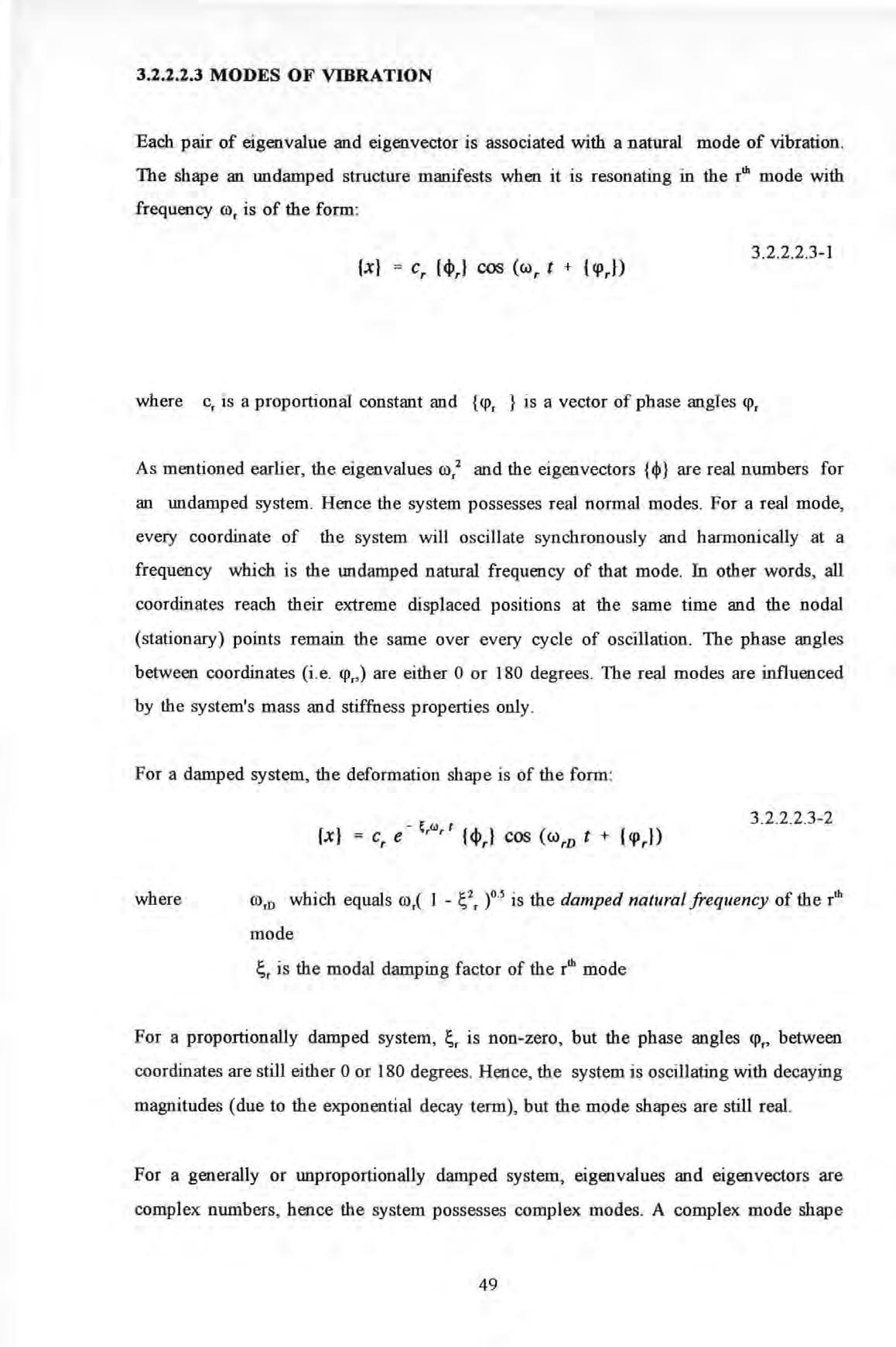
Each pair of eigenvalue and eigenvector is associated with a natural mode of vibration. The shape an undamped structure manifests when it is resonating in the rlh mode with frequency ro, is of the form : where c, is a proportional constant and {q>, } is a vector of phase angles q>,

As mentioned earlier, the eigenvalues ro,2 and the eigenvectors {cl>} are real numbers for an undamped system . Hence the system possesses real normal modes. For a real mode, every coordinate of the system will oscillate synchronously and harmonically at a frequency which is the undamped natural frequency of that mode In other words , all coordinates reach their extreme displaced positions at the same time and the nodal (stationary) points remain the same over every cycle of oscillation The phase angles between coordinates (i .e . q>, ,) are either 0 or 180 degrees. The real modes are influenced by the system's mass and stiffness properties only

For a damped system, the deformation shape is of the form : where ro,0 which equals ro,( 1 - )o.s is the damped natural frequency of the rth mode is the modal damping factor of the rlh mode

For a proportionally damped system, is non -zero , but the phase angles <p, , between coordinates are still either 0 or 180 degrees Hence, the system is oscillating with decayin g magnitudes (due to the exponential decay term), but the mode shapes are still real

For a generally or unproportionally damped system, eigenvalues and eigenvectors are complex numbers , hence the system possesses complex modes . A complex mode shape exhibits a so-called 'galloping effect' i e. some coordinates will reach their extreme displaced positions some times after other coordinates reach theirs. This phenomenon is due to the difference in phase angles between them which are neither 0 nor 180 but somewhere between these two values .

3.2.2.2.4 ORTHOGONALITY OF MODES

In this Section, the mathematical basis of the important orthogonality property which exists between the different modes of vibration is given . The proof is conducted by considering any two modes of vibration : say modes rand s . As for mode r, the natural frequency and the modal vector for mode s should also satisfy Equation 3 .2.2.2.2-8 :

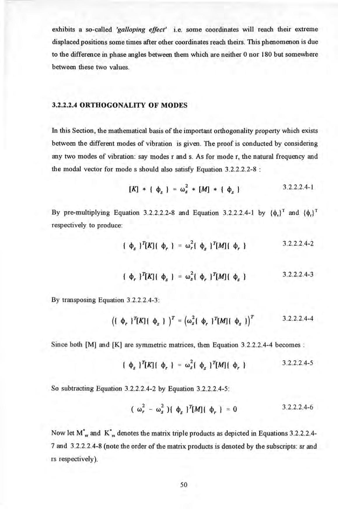
Since both [M] and [K] are symmetric matrices, then Equation 3.2.2.2.4-4 becomes :

Now let M",r and K"r• denotes the matrix triple products as depicted in Equations 3.2.2.2.47 and 3 2 2 2.4-8 (note the order of the matrix products is denoted by the subscripts : sr and rs respectively).

In general , all the natural frequencies of a structure are distinct i e. ror -:1:- ro , then

By following much of the above procedures once more, Equation 3 2 2 2.4-8 1s also obtained :

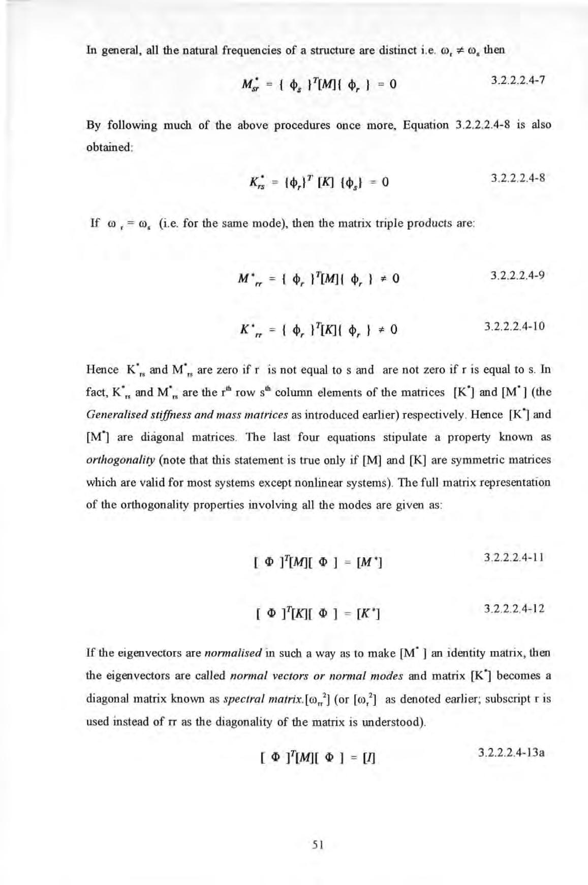
If ro r = ro , (i .e. for the sam e mode), then the matrix triple products are :

Hence K·r. and M•n are zero if r is not equal to s and are not zero if r is equal to s. In fact, K·r. and M·r. are the rth row sib column elements of the matrices [K•] and [M•] (the Generalised stiffness and mass matrices as introduced earlier) respectively Hence [K•] and [Mj are diagonal matrices The last four equations stipulate a property known as orthogonality (note that this statement is true only if [M] and [K] are symmetric matrices which are valid for most system s excep t nonlinear systems) The full matrix representation of the orthogonality properties involving all the modes are given as :

If the eigenvectors are nonna/ised in such a way as to make [M. ] an identity matrix , then the eigenvectors are called nonnal vectors or nonnal modes and matrix [Kj becomes a diagonal matrix known as spec tral matrix. [ro r/ l (or [ror2] as denoted earlier; subscript r is used instead of rr as the diagonality of the matrix is understood).

Recalling Equation 3 .2. 2 .2. 1- 20 :

Using the orthogonality properties , it can be simplified as:

Equation 3 .2 .2.2.4-14 represents a set of uncoupled second order differential equations wlllch are typical of the form (Note : the decoupling of equation of motions in the case of a damped system will be dealt with separately in Section 3.2.2 2 5 ) :

The solution to this equation is already given in Equation 3 .2 .2 .2 .2-7 . So any displacement {x} can be obtained by a weighted superposition of the harmonic motions (of all theN modes) with frequencies equal to the natural frequencies ro, , amplitudes c, and phase angles <p, as stipulated by the equation:

The philosophical importance of the property of orthogonality is that these orthogonal eigenvectors form a basis of the deformation space i .e. any deformation vector can be generated by a linear combination of these linearly independent eigenvecto rs . This statement is known as the expansion theorem which allows modal analysis to be used to obtain the response of a system from the knowledge of the system's modal properties

Orthogonality of modes are often used to check for the consistency of the experimentally measured modal vectors . These modal vectors should, in theory , be orthogonal to each other when weighted with respect to the mass , stiffness or certain limited form of dampin g matrices And as a common practice, the mass matrix is chosen in preference to the other two in testing the orthogonal condition because of the relative ease in determinin g masses

In general , the modal vectors obtained from experiments rarely satisfy Equation 3.2.2 .2.47 . This may be due to errors in measurement, in modal parameter extraction or in the assumed mass matrix. In practice, no alarm should be raised if Equation 3 .2.2.2.4-7 (using nonnal modal vectors) yields a value of not more than 0 1 (with normalisation, the modal mass of each mode has a value of unity)

3.2.2.2.5 APPLICATION OF MODAL ANALYSIS TO NON-PROPORTIONALLY DAMPED SYSTEM

So far, the modal analysis technique (i .e. the technique of decoupling the coupled equations of motion using undamped modal matrix transformation) as applied to undamped systems and systems with a specialised form of damping i.e proportional damping , has been discussed but not systems with the more general forms of damping. Proportional damping assumes that damping is a distributive property like mass and stiffness Such an assumption is not always justifiable especially in situations where heavy localised damping deyjces such as joint dampers , shock absorbers etc are applied to the system For nonproportionally damped systems, the damping matrix [C) cannot be reduced to a diagonal form by means of undamped modal matrix transformation : i.e. [ <I> f * [ C ] * [ <I> ] is not a diagonal matrix

3 2 2 2 5-1

In these circumstances, there are a number of approximation schemes which, in essence, try to retain all the niceties associated with the proportionally damped cases One such scheme is applied in the following ways : let [Cnd] = [<l>f [C] [<I>]

3 2 2 2 5-2 i.e the original system damping matrix is pre- and post-multiplied by [<l>]T and [<I>] to obtain a matrix [Cod ] where the subscript nd denotes non-diagonal . Then a new system damping matrix [Cr ] (where the subscript re denotes reconstruction) is reconstructed by :

3 2.2.2 5-3

The matrix [Cd] is a diagonal matrix which is obtained by retaining only the diagonal terms of the matrix [Cnd1· Another scheme works very much the same way. The matrix [Cod] is reconstructed based on Equation 3 .2 .2.2 .5-4 : where ro. ] is a diagonal matrix constructed from known modal damping factors and undamped natural frequencies ro • .

Once [C.c ] is obtained, it will be used instead of the original system damping matrix [C] and the whole cycle of analysis will be repeated once more The rationale behind thes e schemes is that coupling can be considered as secondary effects and dropping of the offdiagonal terms do not introduce serious errors These techniques can be used in situations where damping l evel is light.

F or systems with hysteretic damping , the analysis procedures are now explained . Recalling that the energy loss per cycle of cyclic stress-strain variation is a measure of damped or dissipated energy For hysteretic damping material s, this energy is found to satisfy the eq uation : where a is a proportional constant independent of frequency of harmonic oscillation

X0 is the di splacement amplitude of oscillation

Similarly, the energy loss for viscous damping materials is found to be : where .Q is the frequency of harmonic oscillation c is the viscous damping coefficient

Hence, for the harmonic excitation case, a structurally damped system may be treated as a viscously damped system with an equivalent viscous damping coefficient which is inversely proportional to the frequency of oscillation. Recalling the equation of motion for a viscously damped system :

If excitation {f} is harmonic (i e {f} = {F0 }ei01 ) then the response {x} is also harmonic (i e. {x} = {X0 }ei01 ) provided the system is linear Now for every hysteretic damping coefficient a;j, it is transformed to an equivalent viscous damping coefficient c0 :

By introducing the coefficients of structural damping Yu :

Then Equation 3 2 2.2 5-11 becomes :

In the general hysteretic damping cases , Equation 3 2 2 2 5-13 cannot be decoupled via the linear transformation using the undamped modal matrix . However, ifthehysteretic damping matrix [yk] (often denoted as [H]) is further assumed as proportional to the stiffness matrix , then all Y;j have the same value i.e. Yu = y .

Equation 3 .2.2.2.5-14 can be decoupled by the linear transformation using the undamped modal matrix (i e {X0 } = [<I>] {11 0 } and {11} = {11 0 }d0 ' is also harmonic) :

Hence based on the orthogonality properties, a set of uncoupled equations are obtained :

Equation 3 .2.2.2.5-16 can be treated as a set of decoupled equations of motion for a system whose stiffness [K] term is replaced by a complex stiffness term ( 1+ j y) [K]. Such analytical expedience has lent itself more popularity amongst some sections of the modal analysis community.

For generally or non-proportionally damped system, then the decoupling technique using the real-valued undamped modal matrix , as discussed so far , cannot be applied. This is because in general , orthogonality of eigenvectors can only diagonalise two matrices at a time (such as [M] and [K] in an undamp ed case). This diagonalisation technique do not work for more than two matrices unless the other matrices (such as [C] or [H]) are linearly proportional to the two matrices [M] and [K]

In the case of a non-proportionally damped system, the solution of the eigenvalue problem is pursued by transforming the second order differential equations (of size N) to one of first order differential equations but having twice the matrix size (i e 2N} or - [A] {Y} + [B] {Y} = {F(t)} where {Y} = , (A] = [: :] , [B) = and {F} =

Equati on s 3 2.2 2 5- 17 are obtained by ad din g a set of auxiliary equations, Equation to the system of equations

The homo geneous solution (corresponding to th e free vibration case i .e . {F(t)} = {0} ) is a formulation for an eigenvalue problem :

B ecause the inverse of (A] is easier to obtain than that of [B] , so the dynamical matrix is expressed as (A]" 1 [B] and not [B]"1 [A]. The eigenvalues are determined by sol ving th e fo llowin g c haracteris tic equation :

This eigenvalue problem formulation has a few similariti es to that of an undamped case: a. [M] and [K] are now replaced by [B] and [A] respectivel y. b The dynamica l matrix [Kr 1 [M] is now replaced by [ Ar 1 [B]. c. The characteristic eq uation of an undamped case is a set of algebraic equations of order N (the total number of degree of freedom of a system) in ro 2 TheN roots ro; 2 ( i = 1, 2 , ,N) are real and positive (because [M] and [K] are real , symmetric and positive definite) Whereas in the generally damped case, the characteristic equation is a set of algebraic equations of order 2N in /.... The 2N roots A; ( i = 1, 2, ... ,2N) are generally complex and the corresponding set of 2N eigenvectors {«!>;•} are also complex The complex damped modal matrix is denoted as [<1>-.J (here the superscript® denotes complex quantities) These eigenvalues must appear as pairs of complex conjugates with negative real parts as depicted in Equation 3 .2 .2 .2 .5-22b :

3 2 2 2.5-22b

H ere ro,( 1 - is often called the damped natural frequency ro,0 Th e corresponding eigenvectors {4>•} must coex.ist and form pairs with their complex conjugates {4>•} • (here { }• denotes a complex conjugate of a vector) d . Ortbogonality , in the case of undamped modal matrix , ensures that the matrix triple products : [<I>] r[M][<I>] and [<I>] r [K][<I>] (all matrices are of size NxN) are all diagonal matrices . Ortbogonality , in the case of complex damped modal matrix, al so ensures that the matrix trip le products : [<I>e_j r [B][<I>-.J (denoted as [Be_]) and [<I>jr[A][<I>j (denoted as [A j) are all diagonal matrices. These matrices are of the size 2N by 2N So the diagonalisation technique using [<I>j can decouple Equations

2 2.2 517 via the transformation : which is a set of decoupled system of equations Once the solution in terms of the modal coordinates {11} is comp lete, then the solution of {Y} (hen ce {x}) can be pursued u sing the expansion theorem as in th e undamped case .

3.3 EXPERIMENTAL APPROACHES OF MODELLING

3.3.1 SYSTEM IDENTIFICATION

System i dentification as in conventional control engineering deals with electro-mechanical systems whose input-output characteristics (transfer functions) are described in : a rational fraction polynomial form or Poles and zeros form where the former and the l atter are roots of the numerator and denominator polynomial respectively or sampled input-output time sequence form with governing parameters such as the orders, delays of the system or Z transform model.

System identification is therefore a process of determining the parameters in these various formulations (a process simi lar to that of the identification of modal and spatial parameters for structural systems as described in Chapters 5 and 6) Because the mathematical model representation in control is quite different from those used in structural engineering, so are the methods of solution However, this distinction h as become increasingly blurred as bilateral transfer between the two technological fields increases.

The introduction of system identification to the field of mechanical structures is briefly reviewed. In 1970, Bekey 13·'1 presented a paper on an introduction and a survey of a numb er of methods for th e identification of general dynamic systems, be they electrical or mechanical He categorized the two different approaches in the tackling of mo st typical engineering problems known as the direct and the inverse approaches. According to his definition, system identification is an inverse approach in which the parameters in the governing equation s are the subjects of determination from the known inputs and th e outputs of a system

Young and On 13 · 111 gave substantial coverage of the general methodology of mathematical modelling of structural systems utilizing experimental vibration data . They detailed the advantages and the disadvantages of a number of identification schemes . In particular to their work, they differentiated two different models which can be derived from experimental data: so-called complete and incomplete models. According to their definition, a complete model is a model which has the same number of degrees of freedom as the number of modes and an incomplete model is otherwise. Further contributions in this particular area are also due to Berman and Flannelly 13"111 They presented a method of deriving incomplete models of mechanical structures . Further coverage on their work wi ll be dealt with in chapter 6

The dynamics of most engineering systems can be treated as linear, second order and time-invariant, at least as a first approximation In fact, these assumptions are necessary for system identification to work . In essence, the technique requues a system (a structure) to be subjected to known input excitations (forces) and the responses (movements at different coordinates of a structure) to be measured The excitations can be any suitable forms : be they periodic , harmonic (sinusoidal) , transient (due to impact) or random

System identification can be categorized as : stochastic/deten11inistic, parametri c/nonparametric, black box or grey box approach and so on . It is beyond the scope of this report to provide a complete coverage on these methods . However, the last two categories are further explained below because of their philosophical importance.

3.3.1.1 THE BLACK BOX APPROACH

A black box approach describes an identification process in which no specific knowledge of the nature of a system IS required. However thi s classification is only conceptually possible. ln practice the black box approach can rarely be applied to reallife other than academic types of problems . Mo st engineering problems do rely on some prior knowledge of the engineering system : be they the form and the order of the governing equations or the values of some of the system parameters etc . Their prior knowledge is often desirable or sometimes even mandatory to obtain a physically realizable solution rather than an imaginary or a mathematical one This modified approach is called the grey box approach

The mathematical models derived using this approach are often called priori models (see Bekey 13·'1 ). This may seem, at fust sight, contradictory to the original requirement of system identification which is called upon because of the lack of full understanding of a system in the first place. It is due to these seemingly conflicting conditions that such an approach is only to be carried out iteratively The approach adopted in this investigation fall s in thi s category . In particular : a . A structure is ass um e d as a linear, second order and time-invariant system . b The order of the structural matrices is assumed so that the derivation of an acceptable spatially and modally truncated model can be effected c. The structural matrices are assumed to b e either full, banded , diagonal or symmetric. d . The mechanism of damping is assumed to b e eith e r as visco us , hysteretic or even undamped .

Further details will be dis c ussed in chapters 5 and 6 .

3.3.2 IMPLEMENTATION

The implementation of this experimental modelling technique entails two basic steps which are common to and quite independent of the types of analysis methods , be they modal or methods The first step involves the experimental acquisition of the so-called input-output data In this testing phase , responses (outputs) of some specific test points of a structure when s ubjected to a particular form of excitation (inputs) , applied at some other test point , have to be measured. The second step involves data analysis which try to fit the previously acquired data to a postulated priori model. In this analysis phase, some forms of curve-fitting methods (in the form of a computing algorithm) are applied to the data to extract the system's parameter.