5.1.3 SUMMARY

In summary, many of the methods described so far possess certain inherent strengths as well as weakness. The appropriateness of a method depends mainly on the particular situations encountered. Some methods work well in some situations but worse in others Therefore no single method can be a panacea for aJI situations

The brief review has highlighted the often conflicting requirements between the simple and the sophisticated methods, such as : a . the quantity and quality of data required , b the accuracy achieved , c the efficiency of use, d the computational requirement etc

Simple SDOF methods are intuitive to use but slow in operation and require a lot of interaction from an analyst. They are also les s accurate unless remedial measures to account for the residual effects have been taken In contrast, most MDOF methods can be programmed to run almost automatically once the initial estimates have been given to start the process Because very little interaction is demanded from the analyst , these methods are extremely fast and efficient to analyzed a large set of data . Above all, th e MDOF methods are capabl e of providing a consistent set of modal parameters for th e complete set of data for all the test positions . Whereas this is difficult for SDOF methods to do For the very same reason , these methods are also sensitive to discrepancy and inconsistency caused by measurement errors.

MDOF methods requue computers with large memory capacity and high speed of computation for performing the large scale data processing involved . With the advent of computer technology, these requirements which a main frame barely meet a decade or two ago can now be fulfilled by a personal computer.

5.2.1 BACKGROUND

In general , experimental data obtained from fie ld tests are of inferior quality than their laboratory counterparts Field d ata are often noisy and have undesirable frequency reso lut ion because of the severe time constraints in taking measurements . Global MDOF methods are thought to be unsuitable becau se the quality of the field data may not be good en ough to be a consistent set.

The alternative algorithm developed during the course of this work is a direct least-square fitting method The simplicity of the algorithm makes the curve-fitting process more apparent to the lay users and this is considered to be a di s tinct advantage. By performing the pre-treatment of data (as explained in Section 5 . 1. 1.2 ) as a pre-requisite step, the algorithm can yield accuracy comparable with other accurate methods. However the algorithm is never meant to compete on these g round s The algorithm has a few features common with the linear regres s ion method which , to most people, is a very familiar mathematical technique Hence, users can find it comfortable to use In lin e with most SDOF methods in its class, this algorithm is al so based on the usual single-mod e assumption . The method has the following characteri stics (some of these are common to other SDOF methods as well and a re not neces sarily unique to this method) :

1 This algorithm does not rely on any geometri cal forms : circles , straight lines or others , explicitly as a curve-fitting criterion.

2 This algorithm is computationa ll y very si mple, intuitive to use and can be easily implemented in a spread sheet or simp l e hand-held calculator application.

3 . This algorithm does not require the manipulations of large matrices.

4 . No initial estimate i s required to start the calculation process .

5. The determination of dampin g parameters i s totally independent of the other modal parameters so errors in determining one parameter will not accumulated in determining the next one

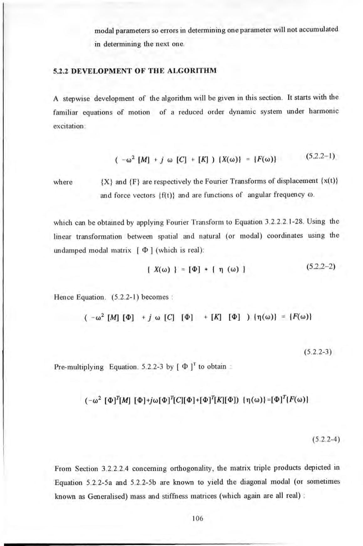
5.2.2 DEVELOPMENT OF THE ALGORITHM

A stepwise development of the a lgorithm will be given in this section . It starts with the familiar equations of motion of a reduced order dynamic system under harmonic excitation : and {F} are respectively the Fourier Transforms of displacement {x(t)} and force vectors {f(t)} and are functions of angular frequency ro which can be obtained by applying Fourier Tran sform to Equation 3 2 2 2 1- 28 Using the linear transformation between spatial and natural (or modal) coordinates using the undamped modal matrix [ <1>] (which is real) :

2 2-1) becomes :

Pre-multiplying Equation 5 2 2-3 by [ <1> f to obtain :

From Section 3 2 2 2.4 concerning orthogonality , the matrix triple products depicted in Equation 5 .2 .2-5a and 5 .2 .2-5b are known to yield the diagonal modal (or sometimes known as Generalised) mass and stiffness matrices (which again are all real) :

If proportional damping is assumed, then (C) can be diagonalised by the undamped modal matrix in the way as stipu lated in Equation 5 .2 .2-5c : where [C*] is the diagonal modaJ or generalised damping matrix .

The modaJ force vector ts gtven as :

In effect, Equation (5.2 2-6) represent a set of uncoupled equations of motion since the modal mass, stiffness and damping matrices are all diagonal matrices The matrix

Equation (5 2.2-6) can be re-written as a set of scalar equations for each mode : (5.2.2-7) where i = 1, 2, 3 .... so on and refers to the mode No.

Within a narrow frequency band close to roi , if the response X , at nodal point s is pre-dominantly contributed by the ith mode, i e residuaJ effect from out-of-range modes is neglected, then : and if there is only one excitation force if receptance a is defmed as :

K '; and C'; can be obtained similarly by dividing K.; and c·; with respectively .

Notice that all M'; , K ; and c·; (called effective mass , stiffness and dampin g) are assumed real . Also since a is a complex quantity and so is its reciprocal (called dynamic stiffness) : (522-14) where

(5 2 2-15a)

(5 .2.2-15b) in which 91 and 3 stand for the real and imaginary parts of receptance respectively . A note of caution must be made here because of the assumption made in arriving at Equation

5 2 2- 9 i e neglecting out-of-range residual effects For an accurate analysis, the residual has to be subtracted from the raw receptance data before inverting them to obtain the dynamic stiffness data Hence by equating the real and imaginary parts of Equation

5 2 2-13 : where A.,(ro) and B,.(ro) are the r eal and imaginary parts of dynamic stiffness respectively .

Or if re-written in matrix form : for n different frequencies close to the ith undamped natural frequency :

If the ith mode is considered dominant within this range of frequencies, then each of these frequencies provide a set of equations, similar in form to Equation 5 2 2-17 : which is of the standard form of mo st system of linear eq uation s.

The dimension of the coefficient matrix [A] is 2n X 3 Since the number of unknowns in this case is only 3, hence a minimum of 3 equations is sufficient for a so lution The solution obtained by using more than this statutory mmunum IS called the pseudo-inverse solution which can be obtained by an application of the following equation

Equation 5 2 2-20 provides an Wlbiased estimate of unknown vector {x} So as the number of frequency points used in the curve-fittin g process increase so does the size of [A]. However it can be shown that the following matrix multiplications can be redu ced to very simple forms : which is only a 3 X 3 matrix Similarly, it can also be shown that :

If data were accelerance (or inertance), revised form ul ae would have to be used The conversion from receptance to accel erance is quite straight forward : where accelerance Yri ro ) is similarly defined as receptance except that acceleration now replaces displacement. Similar to Equation 5 .2 .2-14 , the reciprocal of accelerance is defined as : where A.r and B·,r are simi l arly defined as their A,r and B.r counterparts as the real and imaginary parts of the inverse of accelerance It can be shown that the following equations can be derived:

The solution of the system of equations 5 .2 .2- 23 (of order 3) provide explicit express ions for the three unknowns :

To obtain the various modaJ parameters, the followin g formulae can be us ed : ffi; , and G.r.i are r es p e ctiv ely th e und amp ed n atura l fr e quency, modal damping factor and modal con stants of th e i'h mod e