COMPARISONS OF EXPERIMENTAL AND ANALYTICAL RESULTS

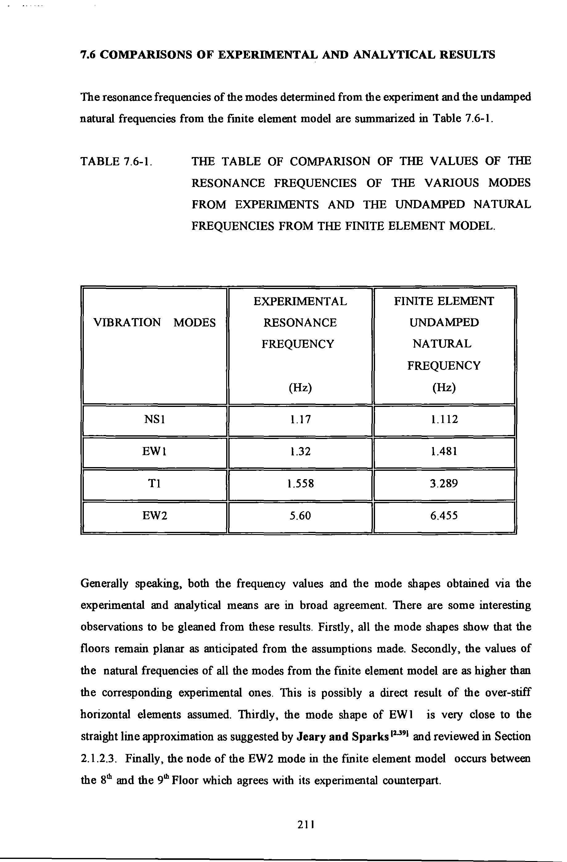
The resonance frequencies of the modes determined from the experiment and the undamped natural frequencies from the fmite element model are summarized in Table 7.6-l. TABLE 7.6-l.

THE TABLE OF COMPARISON OF THE VALUES OF THE RESONANCE FREQUENCIES OF THE VARIOUS MODES FROM EXPERIMENTS AND THE UNDAMPED NATURAL FREQUENCIES FROM THE FINITE ELEMENT MODEL.

Generally speaking, both the frequency values and the mode shapes obtained via the experimental and analytical means are in broad agreement. There are some interesting observations to be gleaned from these results. Firstly, all the mode shapes show that the floors remain planar as anticipated from the assumptions made. Secondly, the values of the natural frequencies of all the modes from the finite element model are as higher than the corresponding experimental ones. This is possibly a direct result of the over-stiff horizontal elements assumed. Thirdly, the mode shape of EW 1 is very close to the straight line approximation as suggested by Jeary and Sparks 11.391 and reviewed in Section 2.1.2.3. Finally, the node of the EW2 mode in the fmite element model occurs between the 81h and the 91h Floor which agrees with its experimental counterpart.

Ambient vibration test technique has rather limited value as far as identification is concerned because the input excitation cannot be measured. Generally, the measured signals (acceleration response) were noisy as reflected by having very low values in the coherence spectra obtained from the experiments carried out. Identifying the appearance of a mode using the criteria of a peak in the autospectra of response is not conclusive. Also very long recording time is required to improve confidence levels of random signals. During the long hours of measurement, undue disturbance can happen and cause disruptive effect as far as accuracy is concerned.

Exciter-induced vibration test usmg a SS or PRBS forcing functions is more useful. However, the level of response obtained may not be as high as its ambient counterparts. SS test is in general very time intensive. The PRBS test is a better technique for field testing as far as the time saving is concerned. With good care in carrying out the signal processing : sampling, filtering, windowing, averaging etc, a PRBS test can produce very good results. This was reflected by the higher values in the coherence spectra obtained from the experiments carried out.

For common building structures, the natural frequencies and mode shapes recommended by the various design literature are close approximations to the experimental ones. They can be used as estimates if no other experimental data is available.

The FE modelling of the BR building carried out was very demanding on the computing resources in carrying out the calculations and producing the analytical results. In general, the undamped natural frequencies from the FE models are close to but consistently higher than the experimental ones. However, the order of occurence of the analytical modes (in ascending order of their natural frequency values) are the same as the experimental ones.

Chapter 8

FULL SCALE FORCED VffiRA TION TESTS OF A FIRE STATION DRILL TOWER

8.1 INTRODUCTION

This chapter reports the results of full scale forced vibration tests conducted on a six storey fire station drill tower. These tests were similar in many respects to those reported in chapter 7 except that the size of this structure was much smaller and more extensive measurements were carried out with the use of the CAT described in Chapter 4. Also much larger amplitudes of response were obtained using the same shaker.

8.2 DESCRIPTION OF THE STRUCTURE

The tower is situated at Camel's Head Fire Station, Plymouth and used for fue fighting training. This structure is simpler in structural form when compared to the BR building but accurate structural modelling of this structure is by no means a trivial task. Structurally, it can be treated as a reinforced concrete frame with most openings partly inftlled with brick walls. The uncertainty regarding the interactions between these walls and the frame accounts for some of the modelling difficulties. Figure 8.2-1 gives a photographic view of the structure.

8.3 TEST ARRANGEMENTS AND PROCEDURES

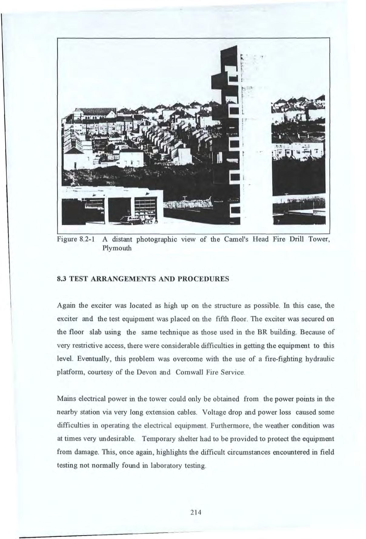
Again the exciter was located as high up on the structure as possible In this case, the exciter and the test equipment was placed on the fifth floor. The exciter was secured on the floor slab using the same technique as those used in the BR building Because of very restrictive access, there were considerable difficulties in getting the equipment to this level. Eventually, this problem was overcome with the use of a fire-fighting hydraulic platform, courtesy of the Devon and Cornwall Fire Service.

Mains electrical power in the tower could only be obtained from the power points in the nearby station via very long extension cables. Voltage drop and power loss caused some difficulties in operating the electrical equipment. Furthermore, the weather condition was at times very undesirable. Temporary shelter had to be provided to protect the equipment from damage This, once again, highlights the difficult circumstances encountered in field testing not normally found in laboratory testing .

The location of the exciter is shown in Figure 8 3-1 Two test series were carried out, each with the exciter orientated in either one of the two principal axes These two directions are designated as EW and NS as shown in Figure 8 3-1

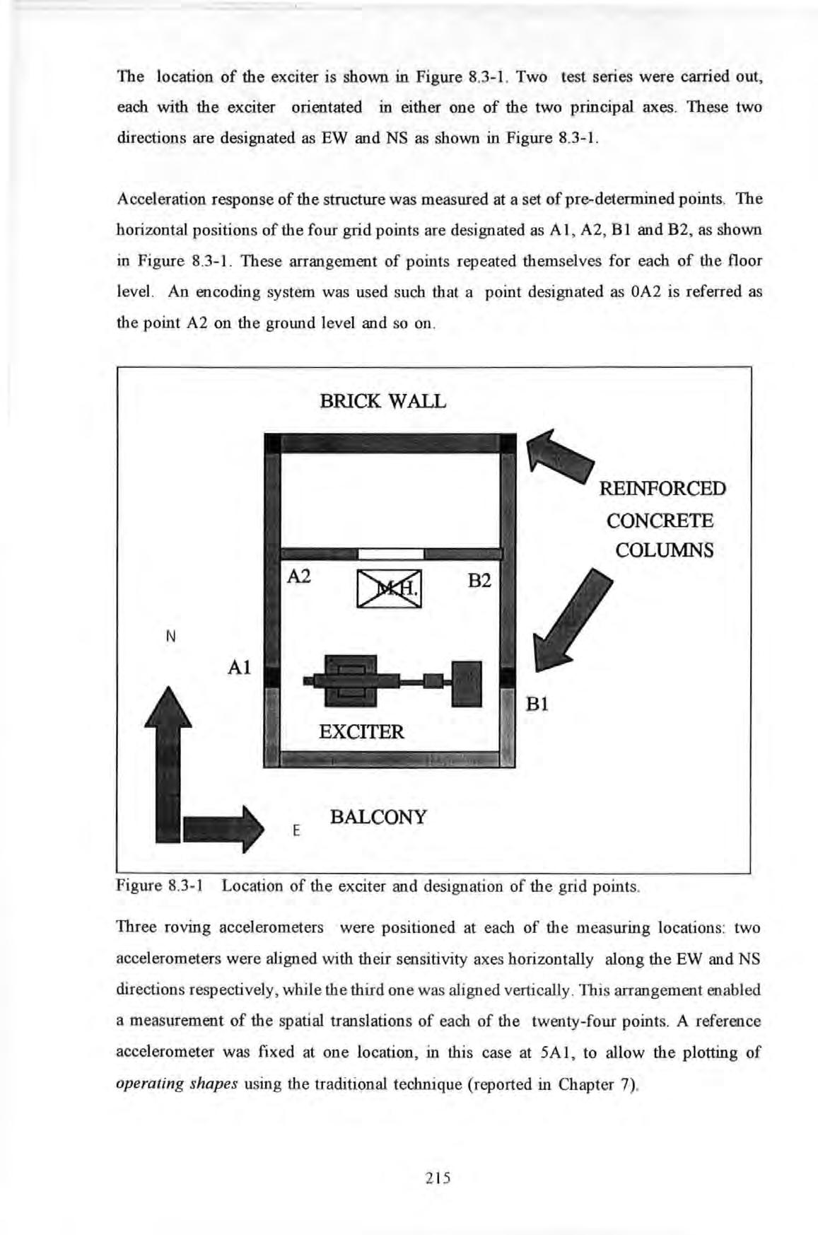
Acceleration response of the structure was measured at a set of pre-determined points. The horizontal positions of the four grid points are designated as A 1, A2 , B 1 and B2 , as shown in Figure 8 3-1 These arrangement of points repeated themselves for each of the floor level. An encoding system was used such that a point designated as OA2 is referred as the point A2 on the ground level and so on .

8.3-1 Location of the exciter and designation of the grid points.

Three roving accelerometers were positioned at each of the measuring locations : two accelerometers were aligned with their sensitivity axes horizontally along the EW and NS directions respectively , while the third one was aligned vertically . This arrangement enabled a measurement of the spatial translations of each of the twenty -four points . A reference accelerometer was fixed at one location, in this case at SA I , to allow the plotting of operating shapes using the traditional technique (reported in Chapter 7).

The inertance and transmissibility measurements were obtained from tests carried out using Pseudo-Random-Binary-Sequence (PRBS) and Step-Sine (SS) excitation. As before, the SS tests with fine steps were only carried out for locating the resonance frequencies of the modes. The bulk of the inertance and transmissibility FRF measurements were taken using PRBS excitation. The spectrum analyzer used was set in the 25 Hz baseband when taking these measurements. This setting provided a frequency resolution of 0.2 Hz. A limited number of zoom measurements with a 0.04 Hz resolution were also taken. Inertance measurements were taken to provide data for modal parameter determination. Transmissibility measurements were taken to determine the operating shapes of the tower under the action of the shaker and at each of the tested frequencies.

Each test was encoded by a Test-Identification (TI) code which provide a unique reference to the location of measurement and other relevant test conditions. A schedule detailing the various test runs and the corresponding TI codes is given in Appendix 8.3.

8.4 TEST RESULTS

The success of incorporating the CAT produced a large collection of data which required quite elaborate data processing efforts involving desk-top PC as well as an IBM main frame computer. Only a representative sample of the results of this analysis is presented below. The results from the SS tests are given first and followed by those from the zoom PRBS tests. The results of the modal parameters determined using data from the 25 Hz baseband are also given.

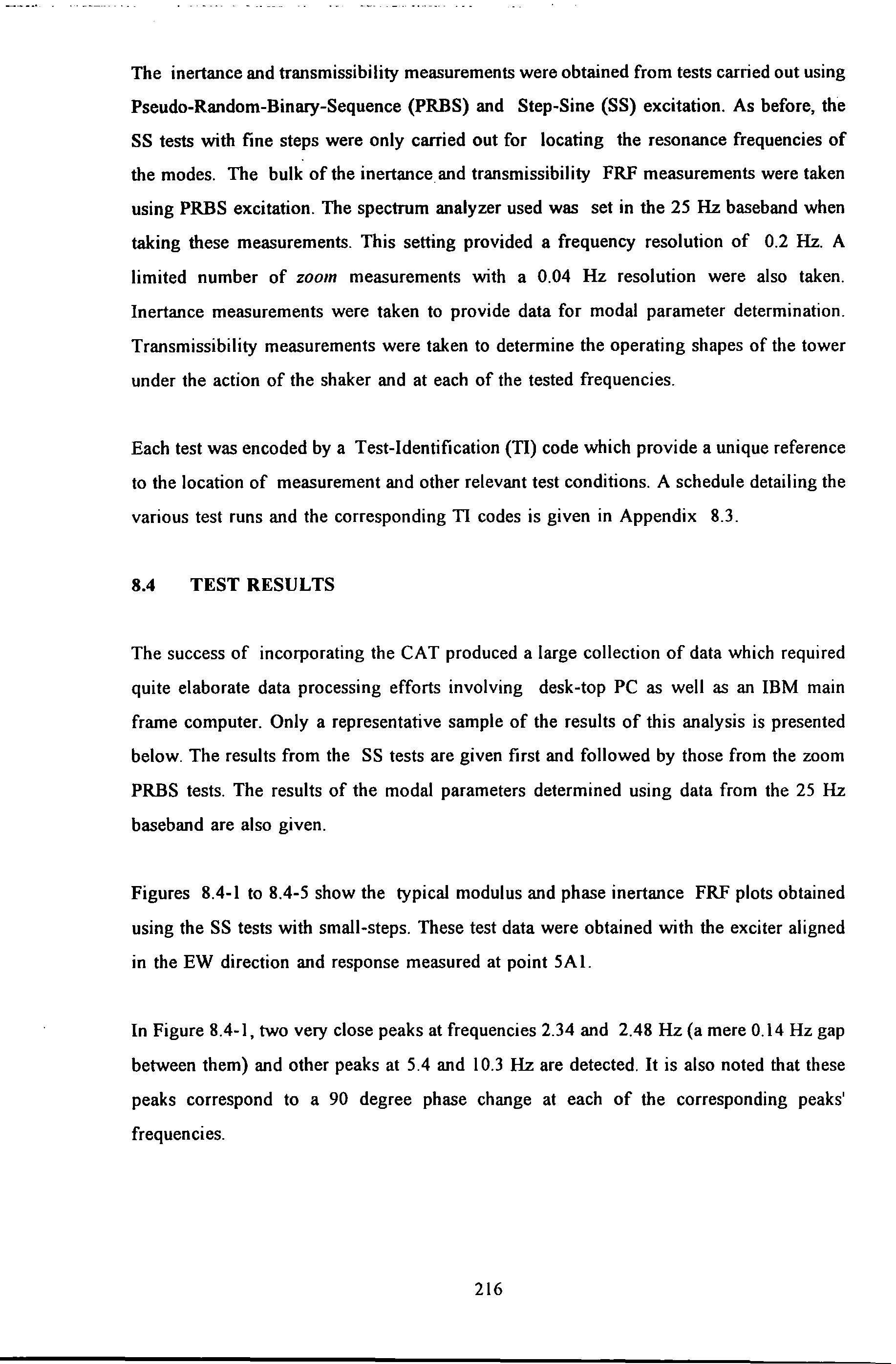
Figures 8.4-l to 8.4-5 show the typical modulus and phase inertance FRF plots obtained using the SS tests with small-steps. These test data were obtained with the exciter aligned in the EW direction and response measured at point SAl.

In Figure 8.4-l, two very close peaks at frequencies 2.34 and 2.48 Hz (a mere 0.14 Hz gap between them) and other peaks at 5.4 and I 0.3 Hz are detected. It is also noted that these peaks correspond to a 90 degree phase change at each of the corresponding peaks' frequencies.

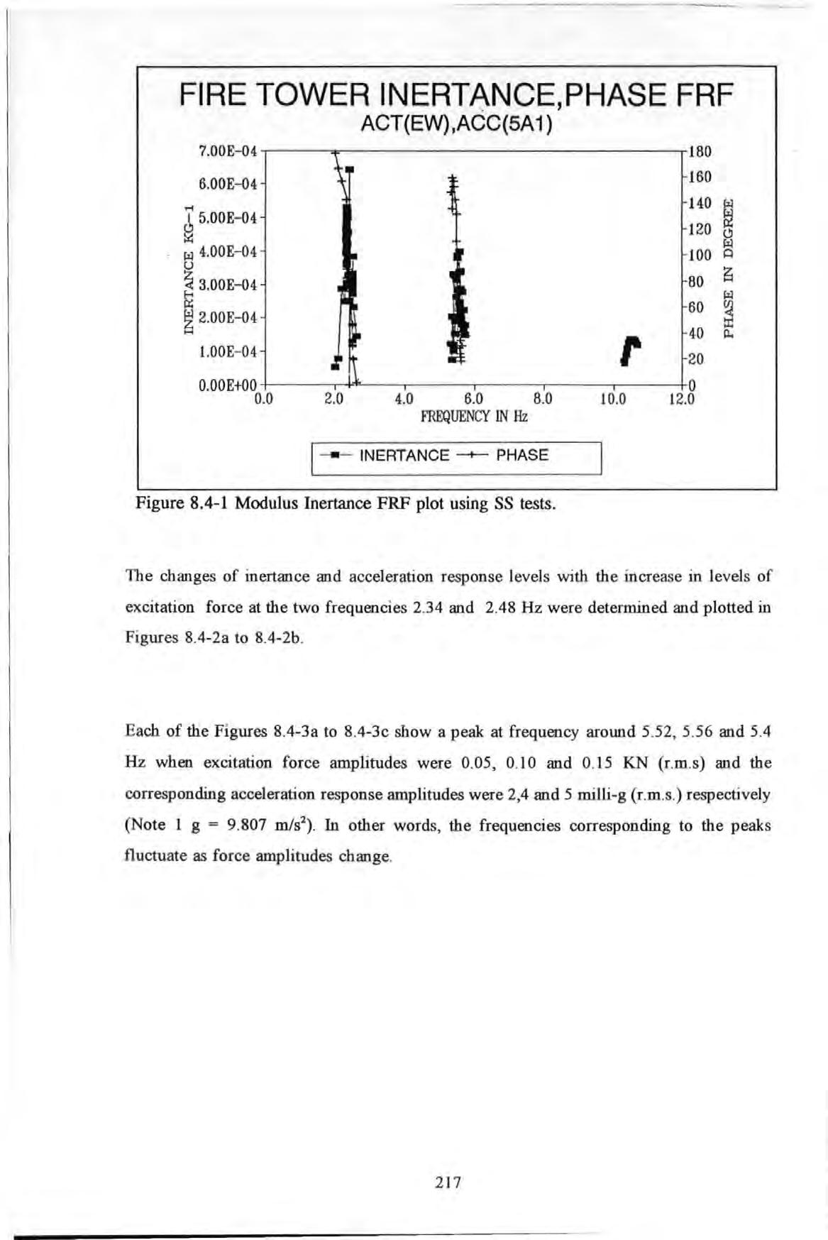
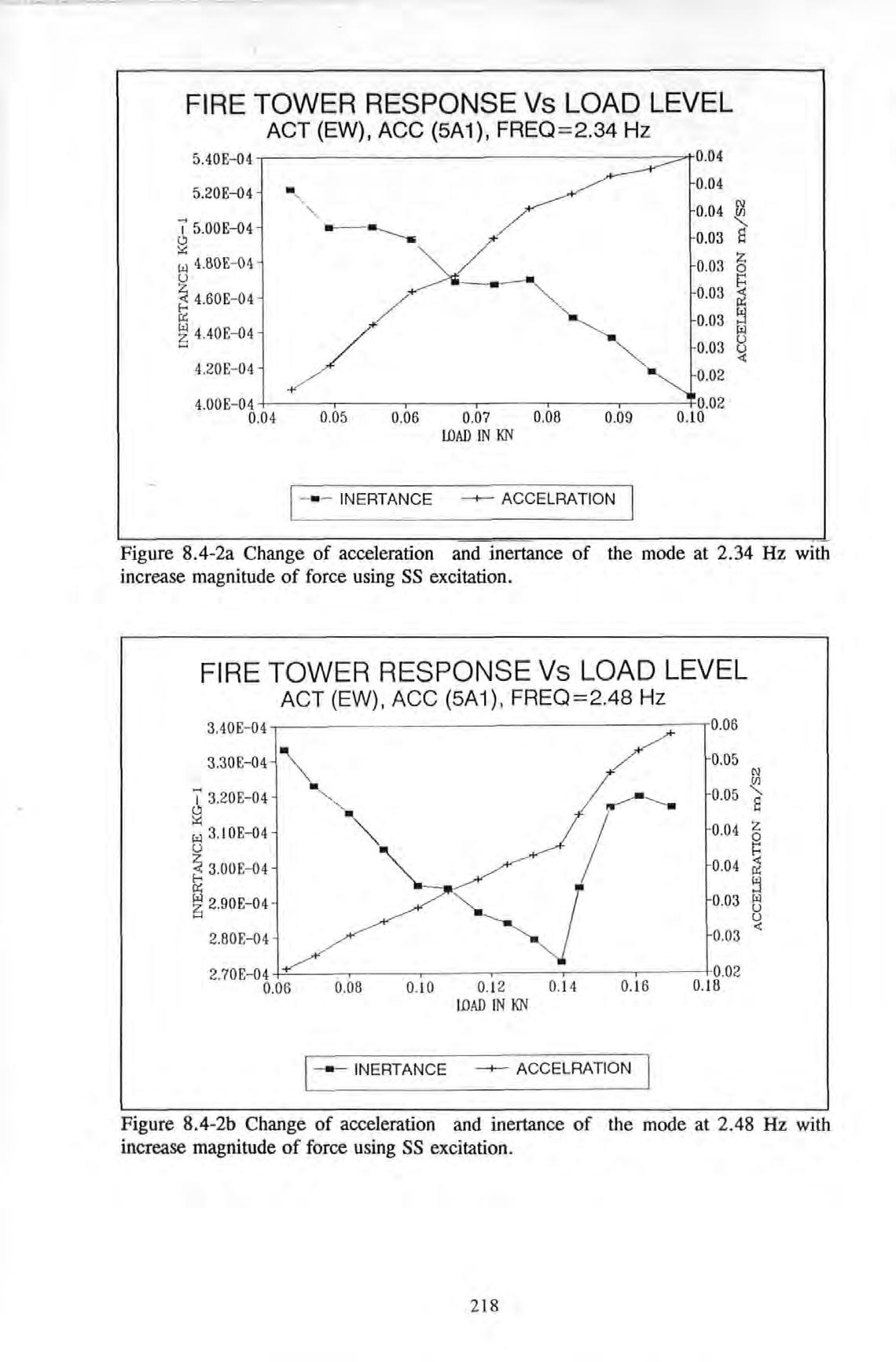
The changes of inertance and acceleration response levels with the increase in levels of excitation force at the two frequencies 2.34 and 2.48 Hz were determined and plotted in Figures 8.4-2a to 8.4-2b

Each of the Figures 8.4-3a to 8.4-3c show a peak at frequency around 5 52, 5 56 and 5.4 Hz when excitation force amplitudes were 0 .05 , 0 . 10 and 0.15 KN (r.m .s) and the corresponding acceleration response amplitudes were 2,4 and 5 milli-g (r m s ) respectively (Note 1 g = 9 807 m/s2 ) In other word s, the frequencies corresponding to the peaks fluctuate as force amplitudes change and phase inertance FRF plot using SS excitation. Measurement was made at SAl with exciter acti ng in the EW direction and force

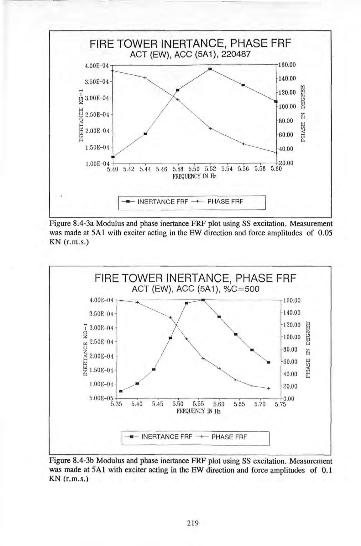
FIRE TOWER INERTANCE, PHASE FRF

Figure 8.4-3c Modulus and phase inertance FRF plot using SS excitation. Measurement was made at SAl with exciter acting in the EW direction and force amplitudes of 0 .15 KN (r.m.s.)

Figure 8.4-4 shows a peak at 10.48 Hz With the exciter acting in the NS direction , the inertance FRF plots obtained are similar to those obtained from the EW direction as regarding the locations of the resonance peaks are concerned . Therefore, they are not to be shown here except the one plotted in Figure 8.4-5 .

FRF plot of the mode at 10.48 Hz using SS excitation. Measurement was made at 5Al with exciter acting in the EW direction

-+----

I

Figure 8.4-5 shows again two very close peaks at 2.36 and 2.46 Hz. This observation agrees with those obtained by the EW excitation. Indeed, the results from the zoom analysis (with a resolution of 0.04 Hz) suggest that there are actually two very close modes: one with a natural frequency at 2.328 Hz and the other at 2.416 Hz (as identified by the algorithm). It is not just the one peak as appeared in all the other measurements taken with a 0.2 Hz resolution. It is clear that the 0.2 Hz resolution, used in the PRBS tests, is not fme enough. However, this is considered a necessary trade-off between resolution and time needed for taking measurements. This 25 Hz baseband setting is necessary in order that all the required measurements can be completed within the short time allowed.

Figures 8.4-6a to 8.4-6c show the inertance FRF spectra taken from the zoom measurements at SAl, with centre frequencies fixed at 2, 5 and 10Hz respectively. In these tests, the exciter was orientated in the EW direction. The corresponding phase inertance spectra are also plotted between 0 and 360 degrees as shown. The results of the analysis are also summarized in Table 8.4-1.

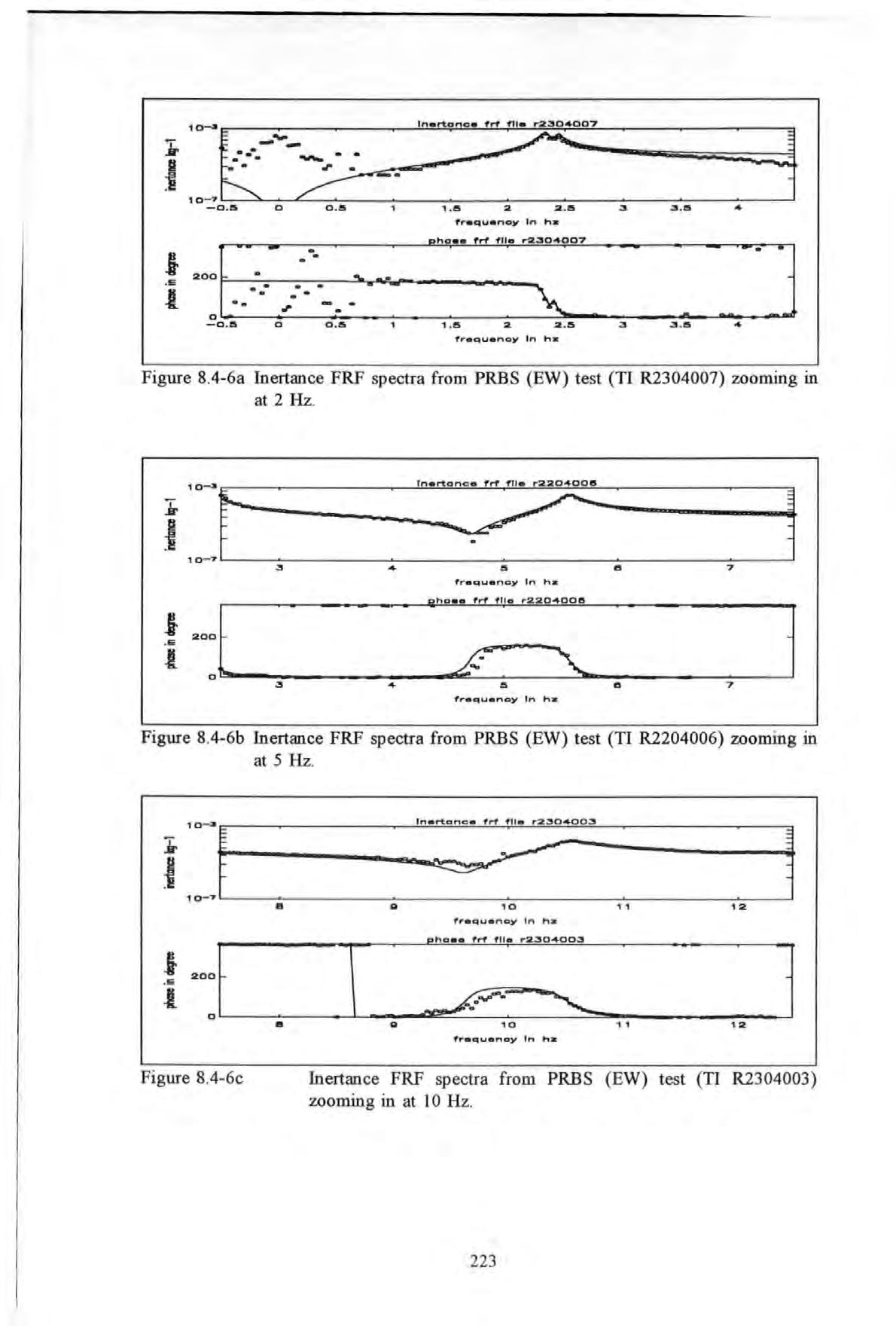
Table 8.4-1: ZOOM ANALYSIS WITH A RESOLUTION OF 0 04 HZ (EW EXCITATION)

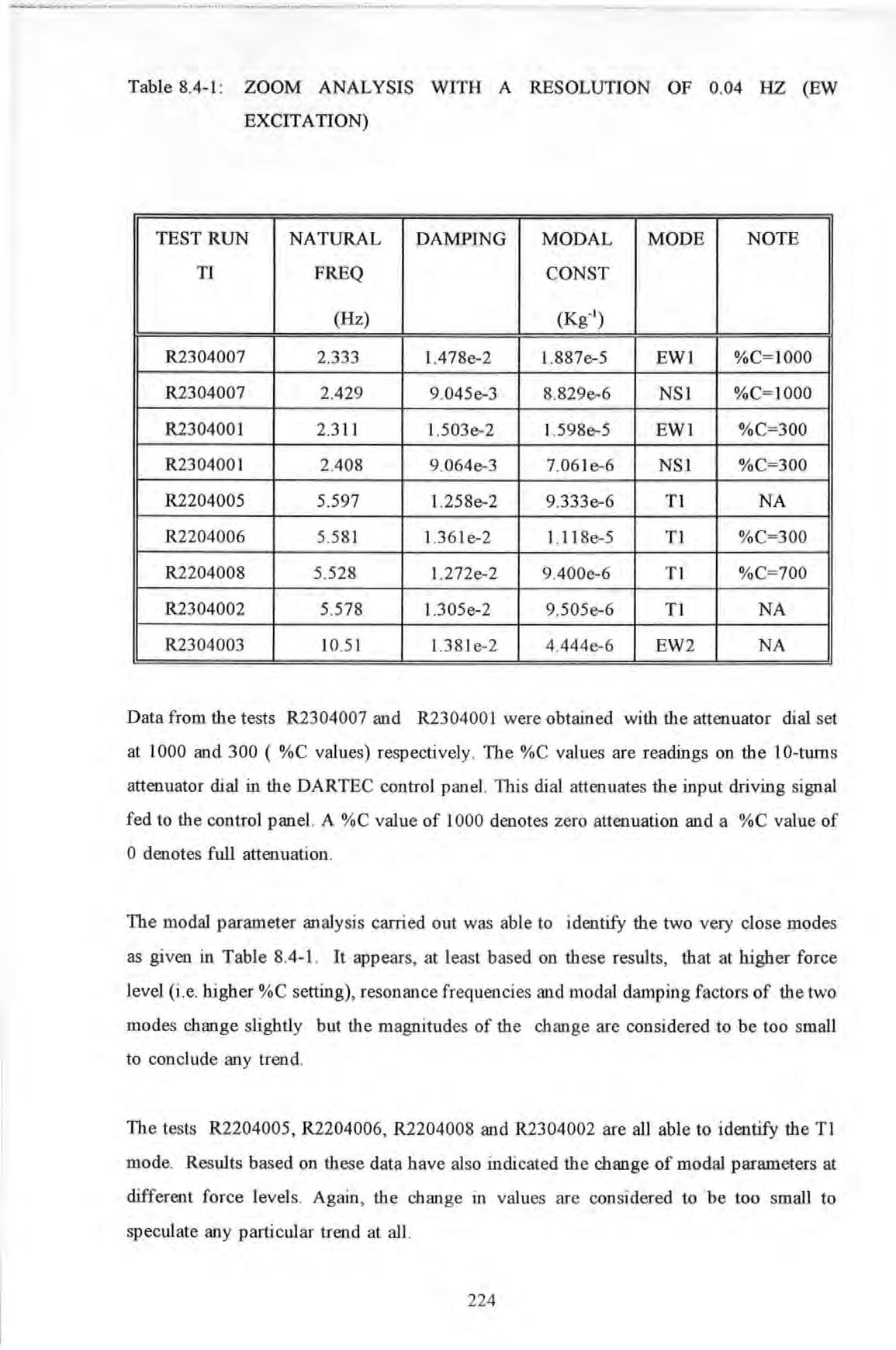
Data from the tests R2304007 and R2304001 were obtained with the attenuator dial set at 1000 and 300 ( %C values) respectively . The %C values are readings on the 10-turns attenuator dial in the DARTEC control panel. This dial attenuates the input driving signal fed to the control panel. A %C value of 1000 denotes zero attenuation and a %C value of 0 denotes full attenuation .

The modal parameter analysis carried out was able to identify the two very close modes as given in Table 8.4-1. It appears, at least based on these results , that at higher force level (i e higher %C setting), resonance frequencies and modal damping factors of the two modes change slightly but the magnitudes of the change are considered to be too small to conclude any trend

The tests R2204005, R2204006 , R2204008 and R2304002 are all able to identify the Tl mode Results based on these data have al so indicated the change of modal parameters at different force levels . Again , the change in values are considered to be too small to speculate any particular trend at all.

Similarly, Figures 8 4-7a to 8.4-7e show the inertance FRF spectra from the zoom measurements taken at 5Al with centre frequencies set at 2, 5, 10, 17 and 25 Hz respectively In these tests, the exciter was acting in the NS direction

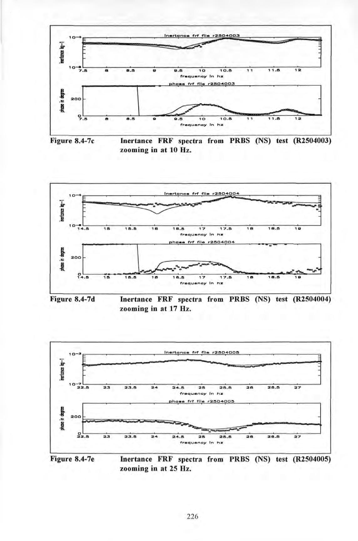
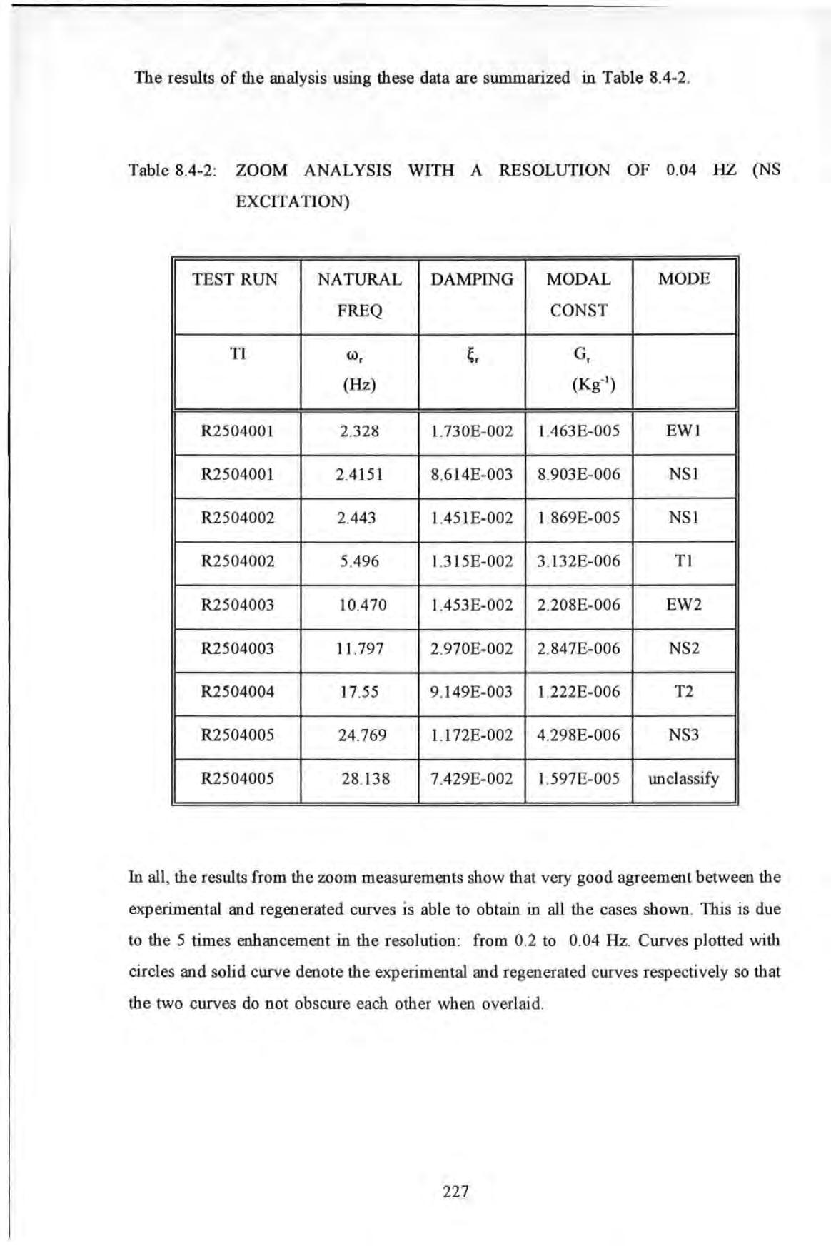
The results of the analysis using these data are summarized in Table 8.4-2

In all , the results f ro m the zoom measurements show that very good agreement between the experimental and regenerated curves is able to obtain in al l the cases shown . This is due to the 5 times enhancement in the resolution: from 0 .2 to 0.04 Hz. Curves plotted with circles and solid curve denote the experimental and regenerated curves respectively so that the two curves do not obscure each other when overlaid

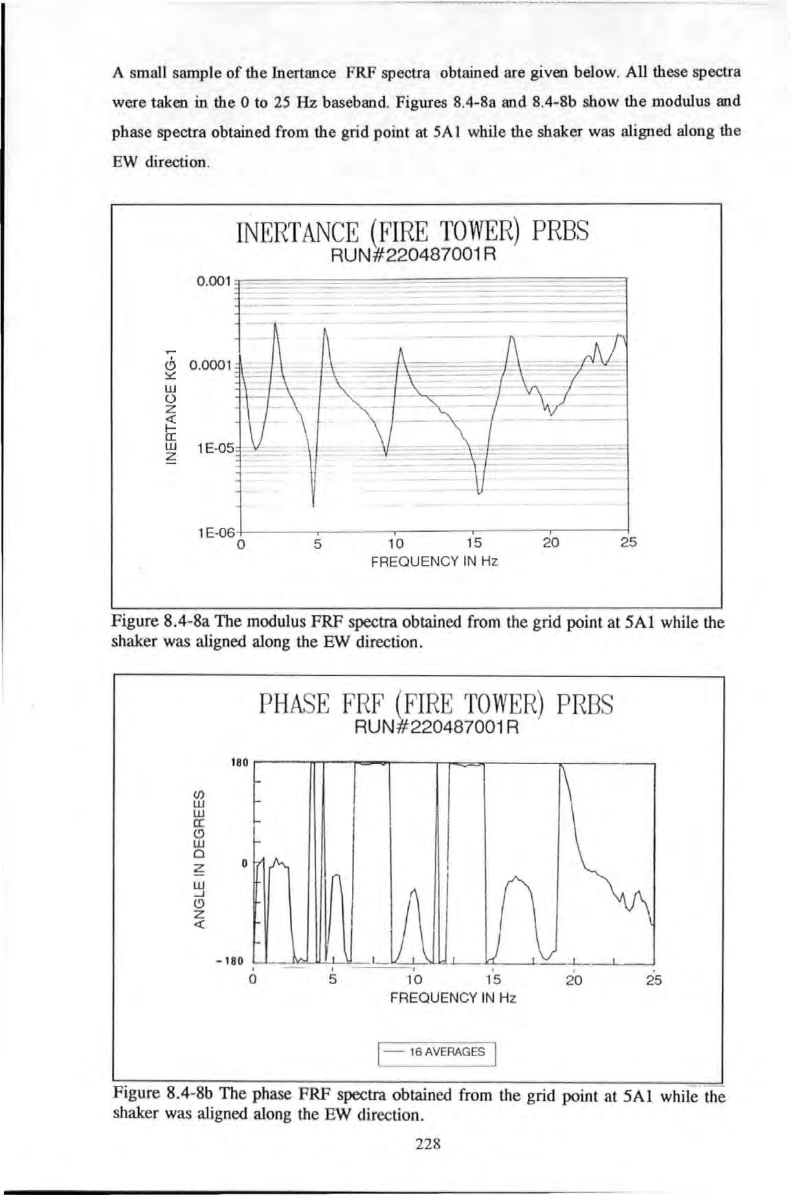
A small sample of the Inertance FRF spectra obtained are given below. All these spectra were taken in the 0 to 25 Hz baseband. Figures 8.4-8a and 8.4-8b show the modulus and phase spectra obtained from the grid point at 5A 1 while the shaker was aligned along the EW direction .

INERTANCE (FIRE TOWER) PRBS

RUN#220487001 R

PH AS E FRF (FIRE TOWER) PRBS

RUN#220487001 R

Figure 8.4-8a shows that, in general, quite distinctive resonance peaks occur at frequencies b elow 17 Hz. But at higher frequencies, modes are heavily 'cramped' together. Because of the dense presences of modes, analyses carried out in the high frequency range will be difficult.

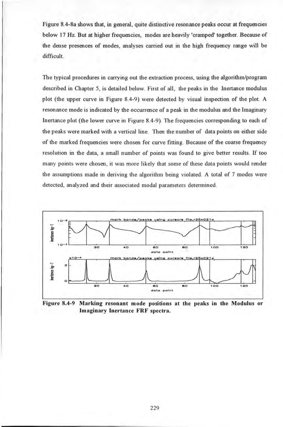
The typical procedures in carrying out the extraction process , using the algorithm/program described in Chapter 5 , is detailed below. First of all, the peaks in the Inertance modulus plot (the upper curve in Figure 8.4-9) were detected by visual inspection of the plot. A resonance mode is indicated by the occurrence of a peak in the modulus and the Imaginary Inertance p lot (the lower curve in Figure 8.4-9) The frequencies corresponding to each of the peaks were marked with a vertical line. Then the number of data points on either side of the marked frequencies were chosen for curve fitting . Because of the coarse frequency resolution in th e data , a small number of points was found to give better results . If too many points were chosen , it was more likely that some of these data points would render the ass umptions made in deriving the algorithm b eing violated A total of 7 modes were detected , analyzed and their associated modal parameters determined .

The experimental and regenerated inertance FRF curves are plotted in Figure 8.4-l 0 for appraisal. Based on the data from the test R25X021X, a good correlation between the two curves is found , especially in the modulus plot. A close examination shows that although the phases near resonance are correctly determined, those near the anti-resonance regions (i .e. between consecutive peaks) are not. This is thought to be due to poor signal-to-noiseratio of measured signals in these regions.

Figure 8.4-11 shows the data and result from the test R25Y023Y (i.e. data taken at grid point 5B2 with the exciter and the accelerometer both aligned in the NS direction) . Again s imilar comments made for Figure 8.4-10 still apply . It is noticed that the phases measured between the peaks are quite erratic. This observation has reinforced the acute requirement for precise phas e measurement

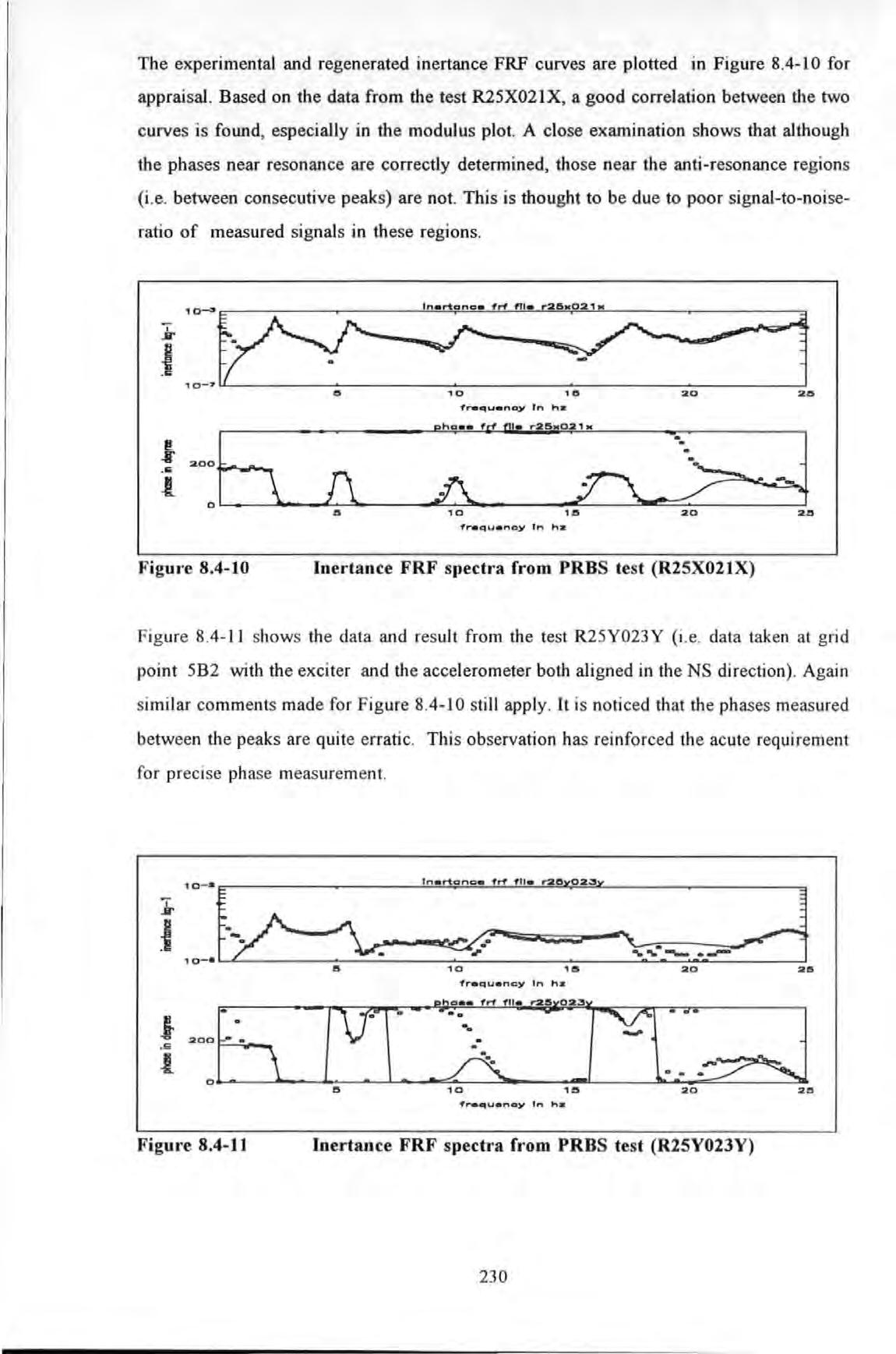
Figure 8.4-12 show the data and result from the test R25Y021X (i .e . data taken at grid point 5A 1 with the exciter and the accelerometer both aligned in the EW direction)

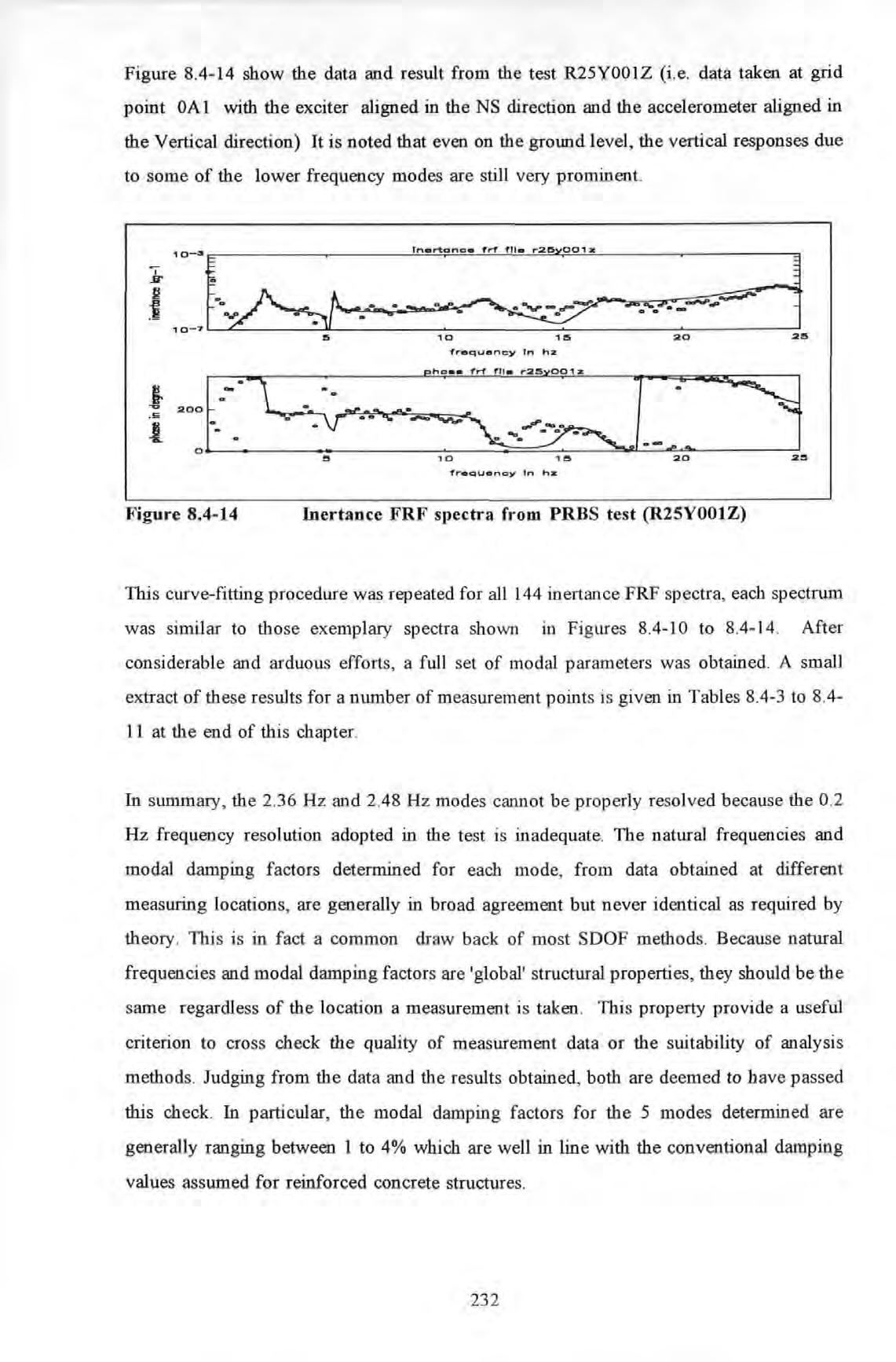
Figure 8.4-13 show the data and result from test R25Y017Y (i .e . data taken at grid point 4A 1 with the exciter and the accelerometer both aligned in the NS direction)

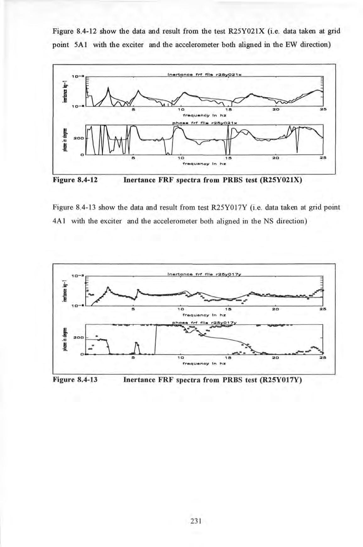
Figure 8.4-14 show the data and result from the test R25Y001Z (i.e. data taken at grid point OA 1 with the exciter aligned in the NS direction and the accelerometer aligned in the Vertical direction) It is noted that even on the ground level, the vertical responses due to some of the lower frequency modes are still very prominent.

This curve-fitting procedure was repeated for all 144 inertance FRF spectra, each spectrum was similar to those exemplary spectra shown in Figures 8.4-10 to 8.4-14 . After considerable and arduous efforts , a ful l set of modal parameters was obtained A small extract of these results for a number of measurement points is given in Tables 8.4-3 to 8.411 at the end of this chapter.

In summary , the 2 36 Hz and 2.48 Hz modes cannot be properly resolved because the 0 2 Hz frequency resolution adopted in the test is inadequate. The natural frequencies and modal damping factors determined for each mode, from data obtained at different measuring lo cations, are generally in broad agreement but never identical as required by theory . This is in fact a common draw back of most SDOF methods . Because natural frequencies and modal damping factors are 'global' structural properties, they should be the same regardless of the location a measurement is taken . This property provide a useful criterion to cross check the quality of measurement data or the suitability of analysis methods. Judging from the data and the results obtained, both are deemed to have passed this check. In particular, the modal damping factors for the 5 modes determined are generally ranging between 1 to 4% which are well in lin e with the conventional damping values assumed for reinforced concrete structures.

The exemplary values of the natural frequencies and modal damping factors of the fust 5 modes determined are summarized in Table 8.4-12

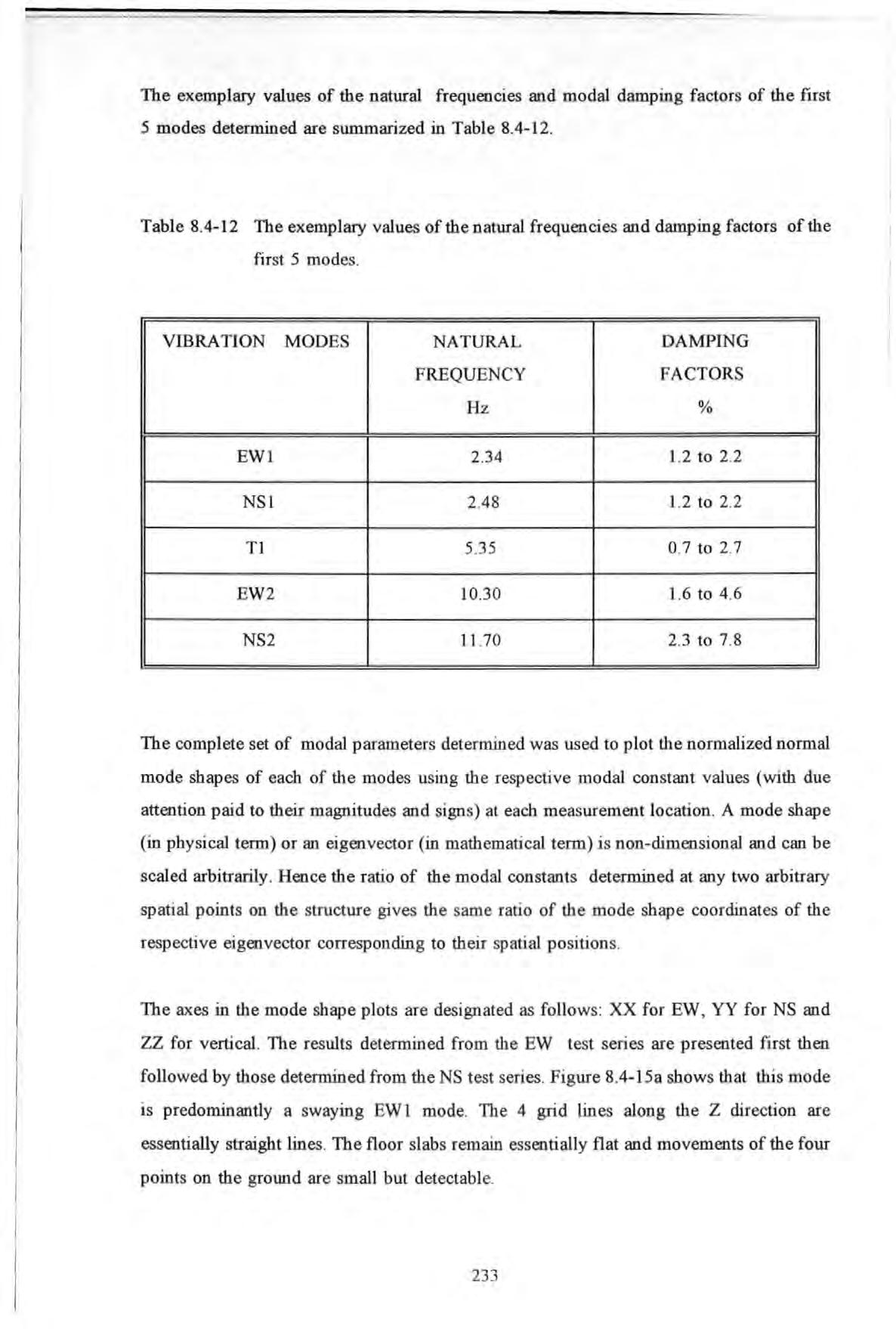
Table 8 4-12 The exemplary values of the natural frequencies and damping factors of the first 5 modes.

Vibration Modes

The complete set of modal parameters determined was used to plot the normalized normal mode shapes of each of the modes using the respective modal constant values (with due attention paid to their magnitudes and signs) at each measurement lo cation . A mode shape (in physical term) or an eigenvector (in mathematical term) is non-dimensional and can be scaled arbitrarily . Hence the r atio of the modal constants determined at any two arbitrary spatial points on the structure gives the same ratio of the mode shape coordinates of the respective eigenvector corresponding to their spatial positions .

The axes in the mode shape plots are designated as fo llo ws : XX for EW , YY for NS and ZZ for vertical The results determined f ro m the EW test series are presented first then followed by those determined from the NS test series . Figure 8.4-15a shows that this mode is predominantly a swaying EW 1 mode The 4 grid lines along the Z direction are essentially straight lines. The floor slabs remain essentially flat and movements of the four points on the ground are small but detectable.

Figures 8.4 - 17 shows the EW2 mode in which a degree of torsional motion is also noted

Figure shows another view of this mode. It appears, but with some reservation, that this may be the second torsional T2 mode

However for the higher frequency modes , it becomes increasing difficult to classify them in the same as the lower frequency modes. For instance, the modes with frequencies around 18 and 24Hz are shown in Figures 8.4-18 and 8.4-19 respectively . As shown in these figures , motions in both the EW and NS directions are of comparable magnitudes and warping of the floor slabs are clearly visible.

Figures 8.4-18c The modes with frequencies around 18 Hz.

Similarly the results from the NS test series are given. Figure 8 .4-20 shows the swaying NS 1 mode. Again , the 4 grid lines along the Z direction are essentially straight lines. Some warping of the floor slabs occurred particularly at the top floor levels. 8.4-20

Figure 8.4-21 shows the torsional T1 mode. However this mode shape is less desirable than those obtained with the shaker acting in the EW direction The movements at the spatial points 4B 2 and 5A1 (points 19 and 21 in the figure) are unconformable to those shown in Figures 8.4-16 possibly owing to experimental errors shows the NS2 mode

The torsional T 1 mode.

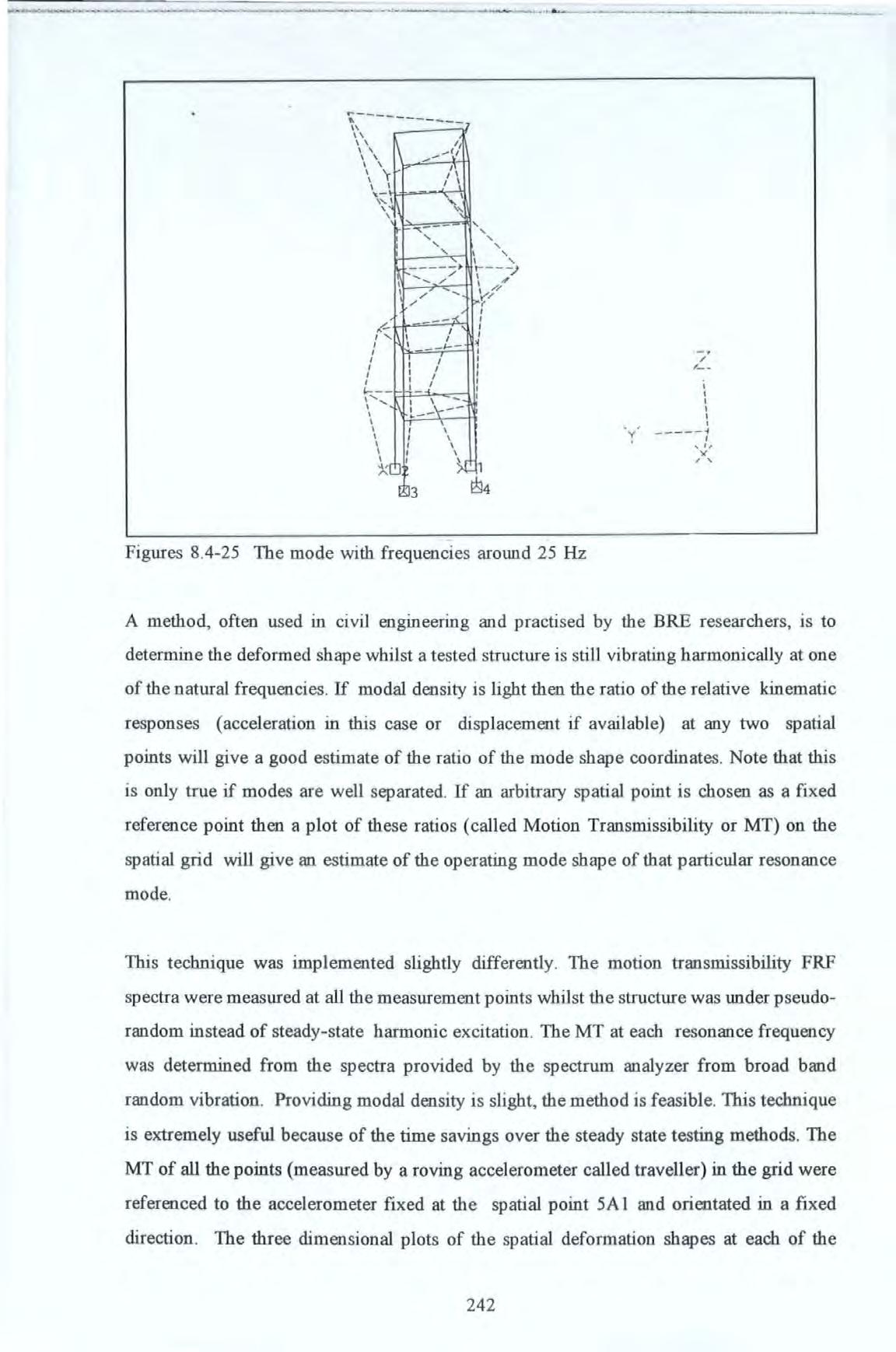
Figures 8.4-23 to 8.4-25 show the three other modes with natural frequencies around 16, 18 and 25 Hz respectively . For the same reasons already described, it is difficult to classify these modes .

Figures 8.4-23 The mode with frequencies around 16Hz

Figures

A method, often used in civil engmeenng and practised by the BRE researchers, is to determine the deformed shape whilst a tested structure is still vibrating harmonically at one of the natural frequencies If modal density is light then the ratio of the relative kinematic responses (acceleration in this case or displacement if available) at any two spatial points will give a good estimate of the ratio of the mode shape coordinates. Note that this is only true if modes are well separated If an arbitrary spatial point is chosen as a fixed reference point then a plot of these ratios (called Motion Transmissibility or MT) on the spatial grid will give an estimate of the operating mode shape of that particular resonance mode

This technique was implemented slightly differently . The motion transmissibility FRF spectra were measured at all the measurement points whilst the structure was under pseudorandom instead of steady-state harmonic excitation. The MT at each resonance frequency was determined from the spectra provided by the spectrum analyzer from broad band random vibration. Providing modal density is slight, the method is feasible This technique is extremely useful because of the time savings over the steady state testing methods The MT of all the points (measured by a roving accelerometer called traveller) in the grid were referenced to the accelerometer fixed at the spatial point 5A I and orientated in a fixed direction . The three dimensional plots of the spatial deformation shapes at each of the resonance frequencies were obtained with the use of the GINO graphic software. Like mode shapes, these plots provide an immensely useful tool to visualize the physics and behaviour of a structure at resonance or other conditions. f = 2.36Hz f = 10.2Hz f = ll.Hz f = 16.7Hz

Figures 8.4-26a to 8.4-26d show the operating mode shapes at 2.36, l 0.2, 11.4 and 16.7 Hz with the exciter acting along the EW direction. There are some resemblances between these operating mode shapes and the corresponding mode shapes presented earlier. However for the two modes with very close natural frequencies, it should be borne in mind that the operating mode shapes will not approximate the true mode shapes.

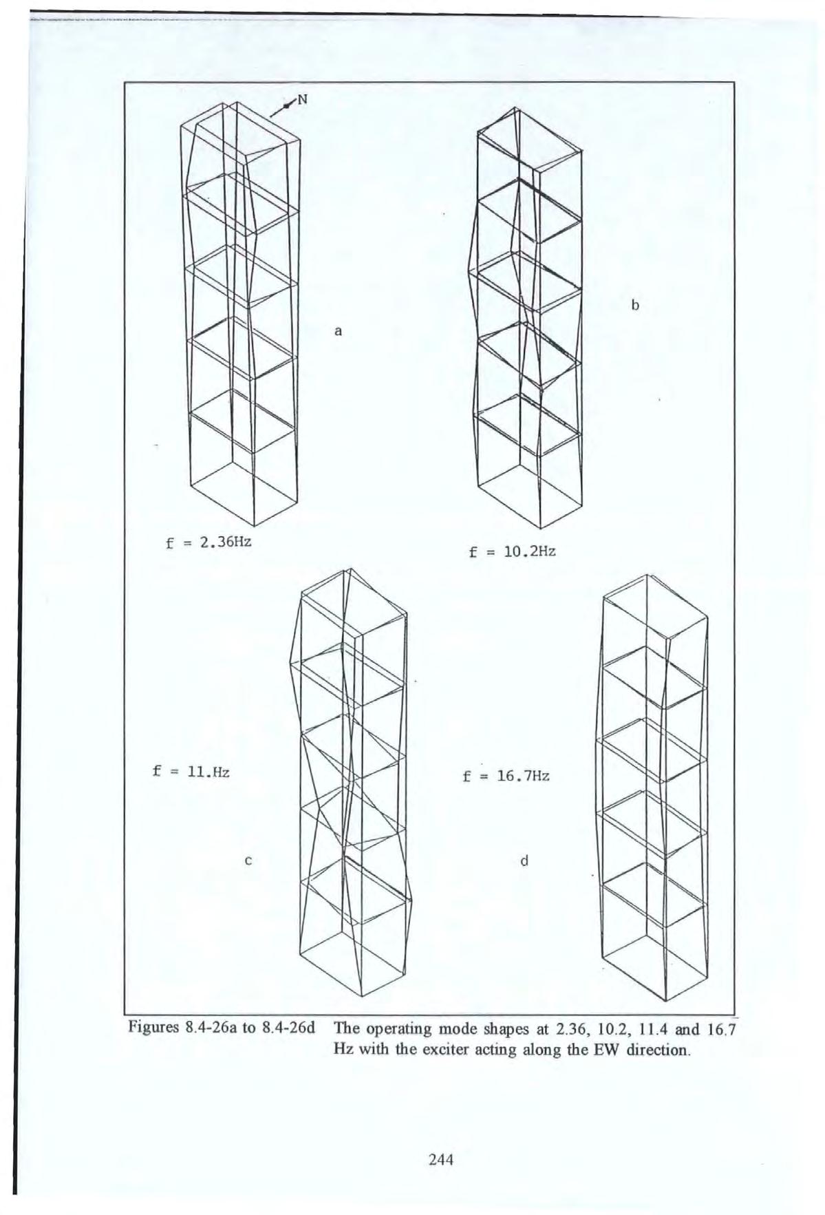
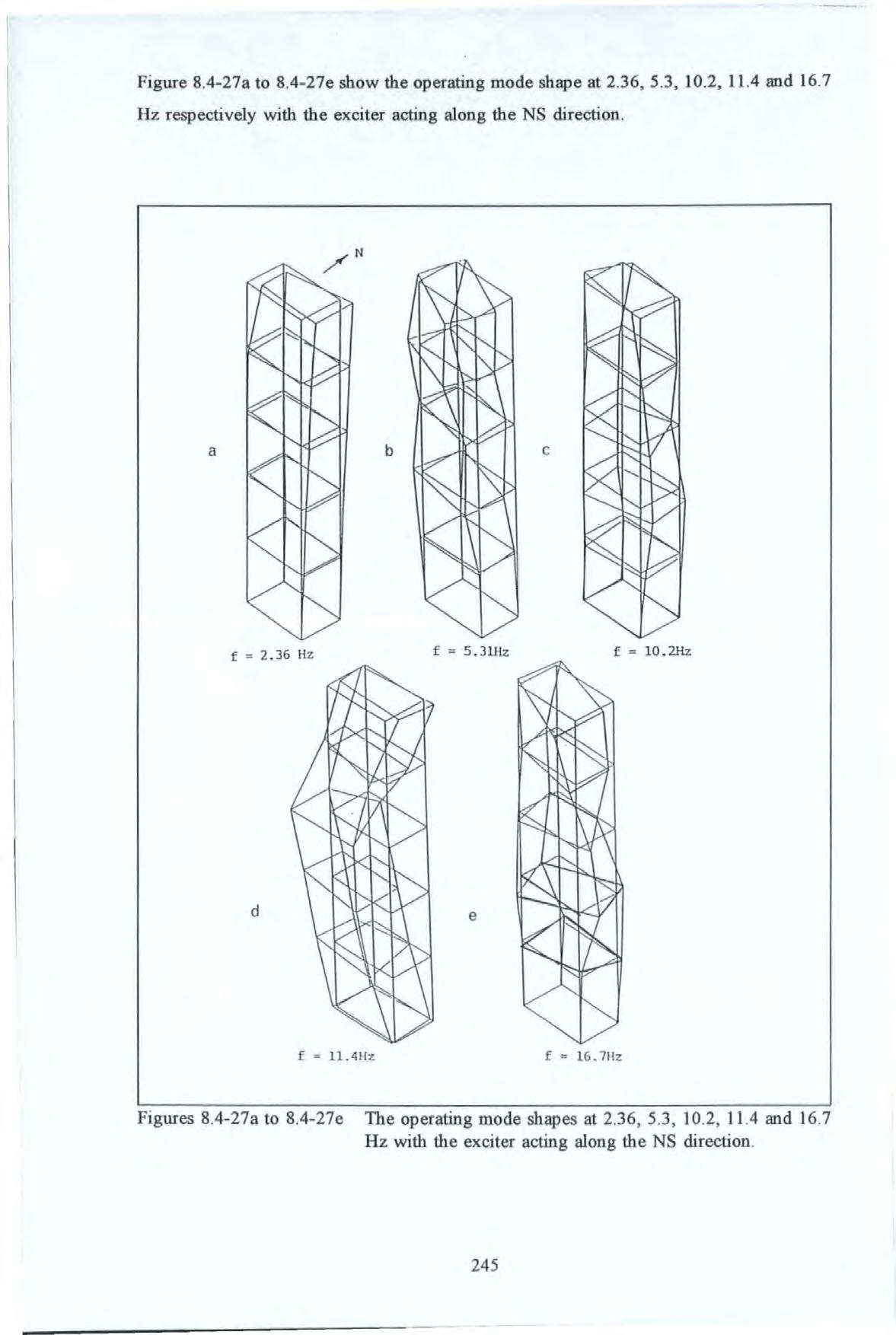
Figure 8.4-27a to 8.4-27e show the operating mode shape at 2 36, 5.3, 10 2, 11.4 and 16.7 Hz respectively with the exciter acting along the NS direction

= 11.4Hz

= 16.71iz where is the natural frequenc y of the rth mode is the modal damping factor of the rlh mode

Figures 8 4- 27a to 8.4-27e The operating mode shapes at 2 36 , 5 3 , 10 2, 11.4 and 16 7 Hz with the exciter acting along the NS ctirection .

The results show that most of the dominant modes of the tower occur below 25 Hz with the fwulamental modes occurring at about 2.3 Hz. The closeness of the EW I and NS 1 is believed to be due to the near symmetry in the structural, not architectural, details along the EW and NS directions. Because of the closeness of these modes, considerable coupling occurred and a mode could be excited even when the shaker was acting in a direction orthogonal to the mode. The torsional Tl mode occurred at a frequency roughly twice that of the fundamental swaying modes. The slightly lower frequency of the EW I mode than that of the NS I mode may suggest that the stiffness reduction due to the openings on one of the two infilled brick walls on the EW plane may be responsible, providing all the other structural factors concerning the walls stay the same in both the EW and NS planes.

All the mode shapes determined show considerable movements in the fifth floor. Hence, the placement of the exciter on this level was appropriate. The damping levels of all these modes are found to be around I% of critical damping. This is considered typical of most reinforced concrete structures and there is no cause for concern of any abnormality on this structure.

Tests results show that the natural frequencies of the Tl mode fluctuate with different force levels. However, due to the lack of sufficient data using SS excitation and insufficient frequency resolution, no conclusive statement can be made regarding the linearity or otherwise of this structure.

Because of the small size of the structure, very large amplitude motions of the structure have been excited. Considerable responses were measurable even at ground level which was five floor levels down from where the exciter was. Because SS tests can be carried out at variable steps, very fme frequency resolutions can be obtained at the expense of time. However, applying SS tests extensively will be too time-intensive and is not suitable to full scale field testing. The PRBS test method is extremely time efficient but cautions must be exercised especially regarding the problem of lack of frequency resolution in data. This is because the PRBS test method produces FRF spectra with a constant frequency resolution across the entire band of analysis. The results obtained in the field tests are largely consistent but are still inferior to those obtained from laboratory. Finally, it is shown that very useful structural information can be determined by performing full scale forced vibration testing on structures.

Table 8.4-3. Modal parameters set determined from test data 220487001R (from 25 Hz PRBS tests with exciter acting EW and measurements made at grid point 5Ai in the EW direction).

Gr is the modal constant of the r 1 h mode

M' is the effective mass of the rlh mode r

C'r is the effective damping of the rlh mode

K' is the effective stiffness of the rth mode r

Table 8.4-4 . Modal parameters set determined from test data 230487009R (from 25 Hz PRBS tests with exciter acting NS and measurements made at grid point 5Al in the NS direction).

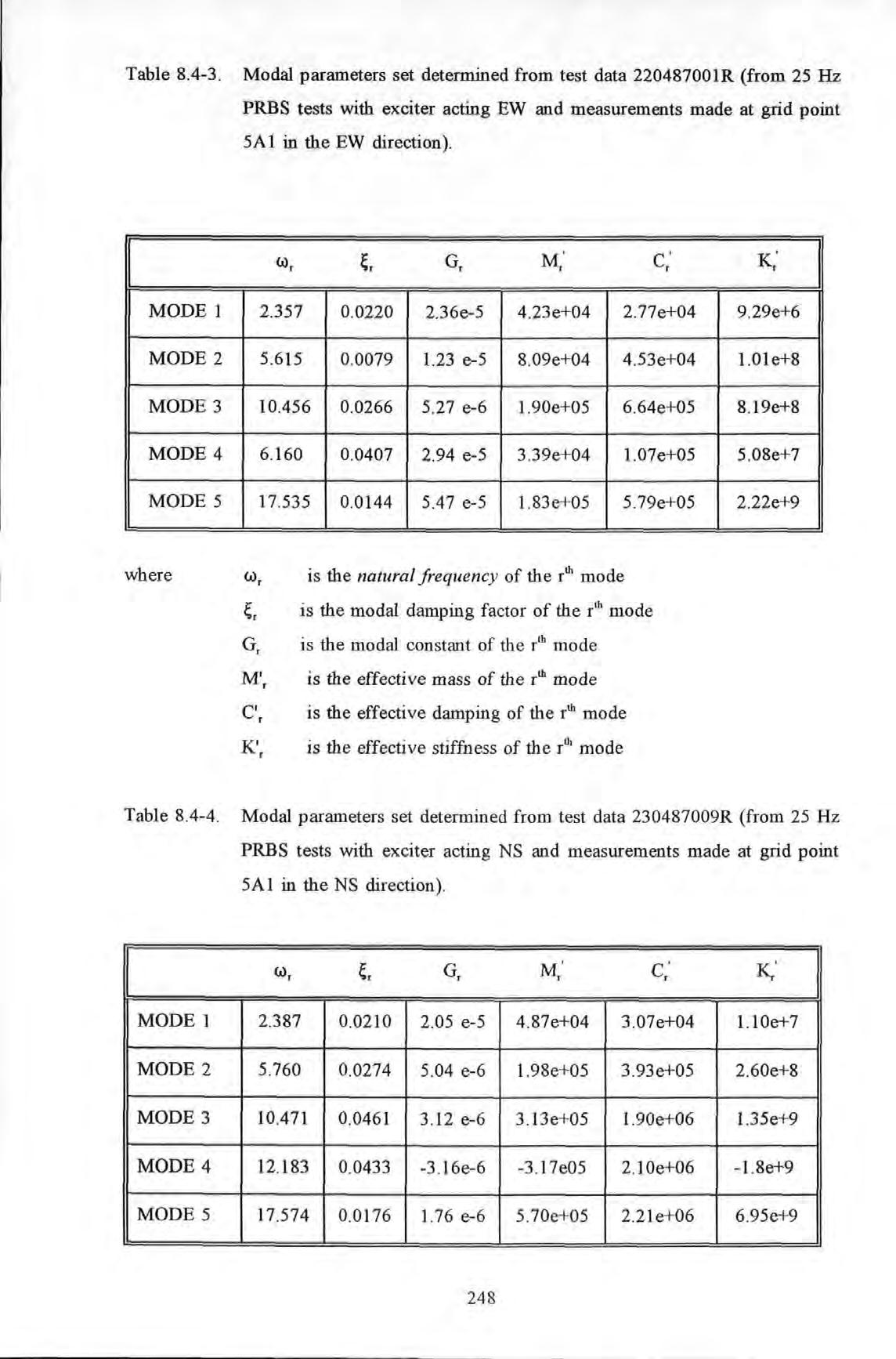
Table 8.4-5 . Modal parameters set determined from test data 250487017 (from 25 Hz PRBS tests with exciter acting NS and measurements made at grid point 5B2 in the NS direction)

Table 8.4-6. Modal parameters set determined from test data 260487008R (from 25 Hz PRBS tests with exciter acting NS and measurements made at grid point 4A2 in the NS direction) .

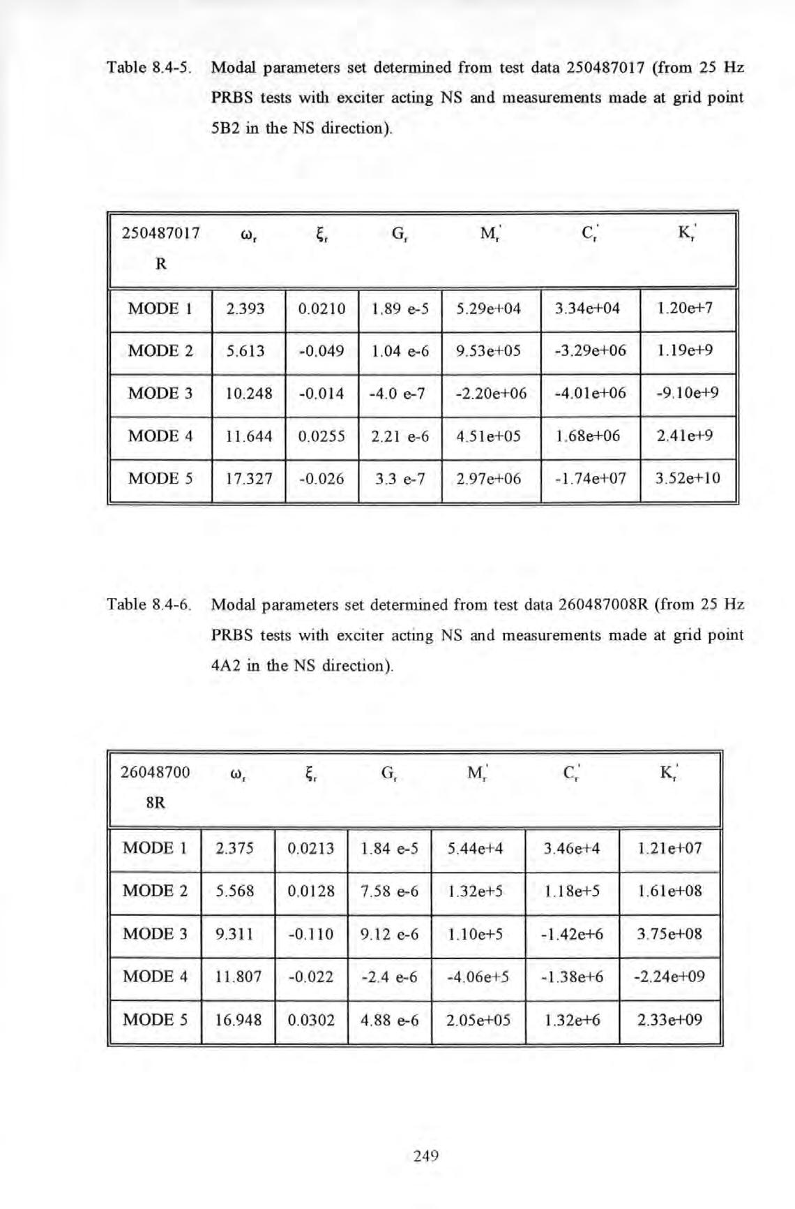
Table 8.4-7. Modal parameters set determined from test data R25X021X (from 25 Hz PRBS tests with exciter acting EW and measurements made at grid p oint 5A2 in the EW direction) .

Table 8.4-8 . Modal parameters set determined from test data R25Y023Y (from 25 Hz PRBS tests with exciter acting NS and measurements made at grid point 5B2 in th e NS direction)

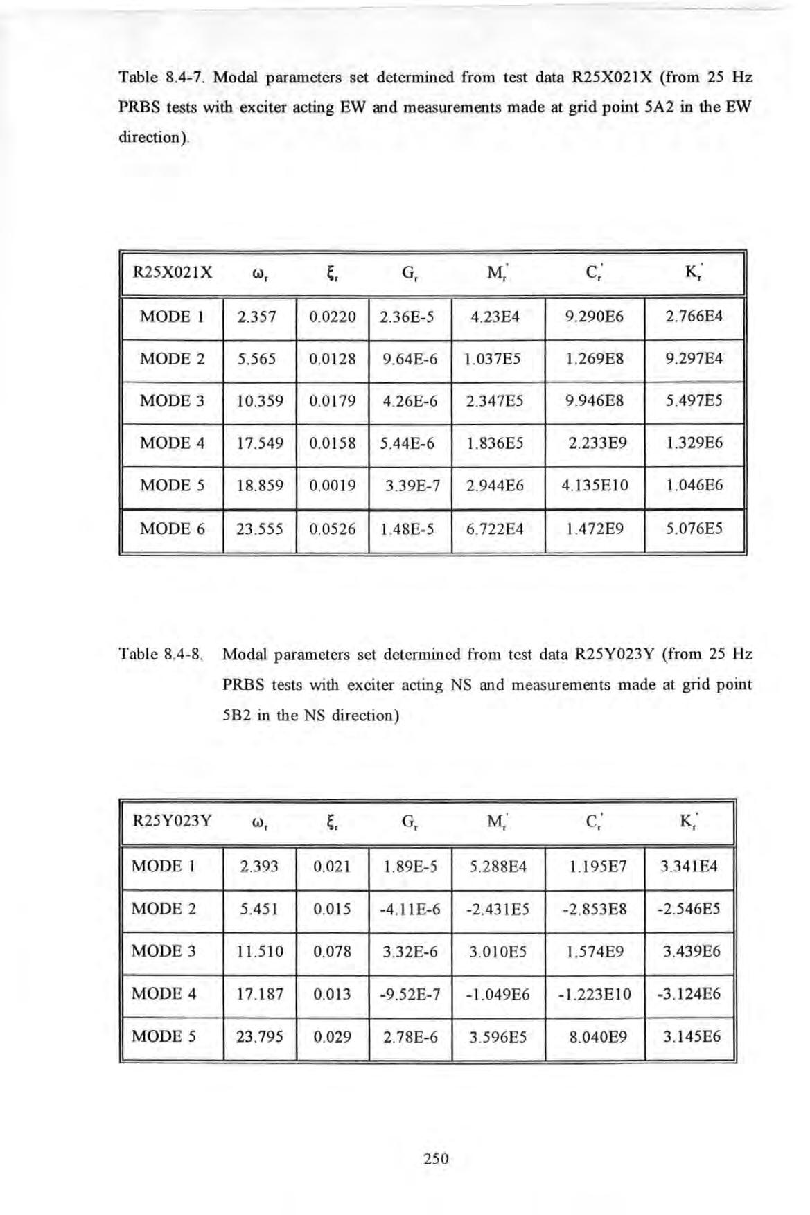
Table 8.4-9 . Modal parameters set determined from test data R25Y021X (from 25 Hz PRBS tests with exciter acting NS and measurements made at grid point 5A2 in the EW direction)

Tab l e 8.4-1 0. Modal parameters set determined from test data R25YO 17Y (from 25 Hz PRBS tests with exciter acting NS and measurements made at grid point 4A 1 in the NS direction) .

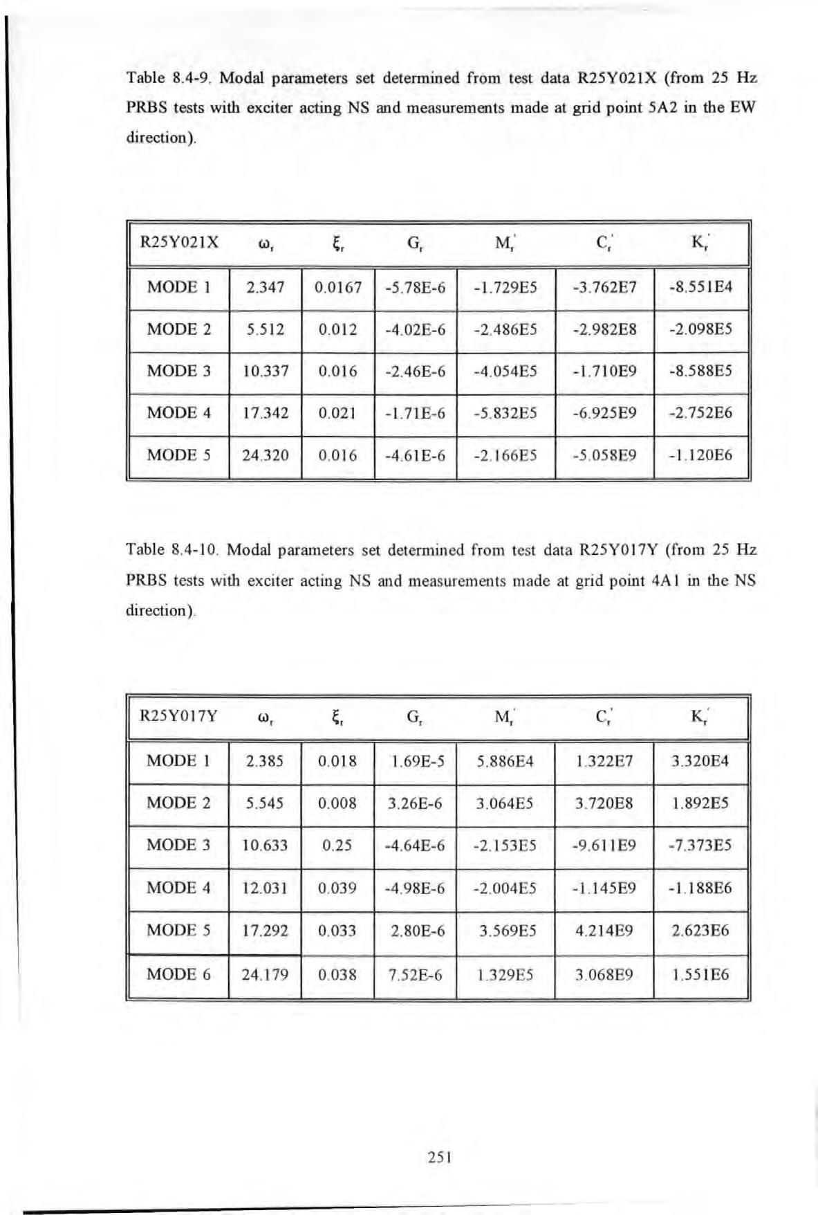
Table 8.4-11. Modal parameters set determined from t es t data R25Y001Z (from 25 Hz PRBS tests with exciter acting NS and measurements made at grid point OAl in the Vertical direction)