5.3 IMPLEMENTATION AND VERIFICATION

The algorithm was implemented in a numb er of computing environments and platforms :

Hewlett Packard HP Basic® Version 4

MA TLAB ® routines and spread sh eet application in QUA TIRO PRO®.

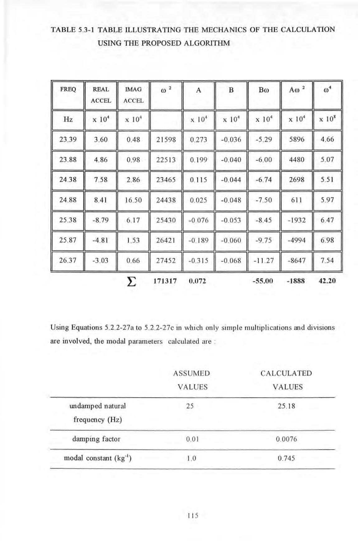
The mechanics (not accuracy since values a re roWlded off to fit in the t ab l e) of the calculation at work can be illustr ated by the following example (usin g the synthesi zed data of the four-mode fictitious system to be described below) :

TABLE 5.3-1 TABLE ILLUSTRATING THE MECHANICS OF THE CALCULATION USING THE PROPOSED ALGORITHM

Using Equations 5.2 2- 27a to 5 2 2-27c in w hi ch onl y si mp le multiplications an d divisions are involved , the modal parameters calcul at ed are :

The discrepancy is due to rounding errors in the initial input data (accelerance values etc) and in performing the calculation . Also it is due to the fact that removal of residual effect from the data has not been performed .

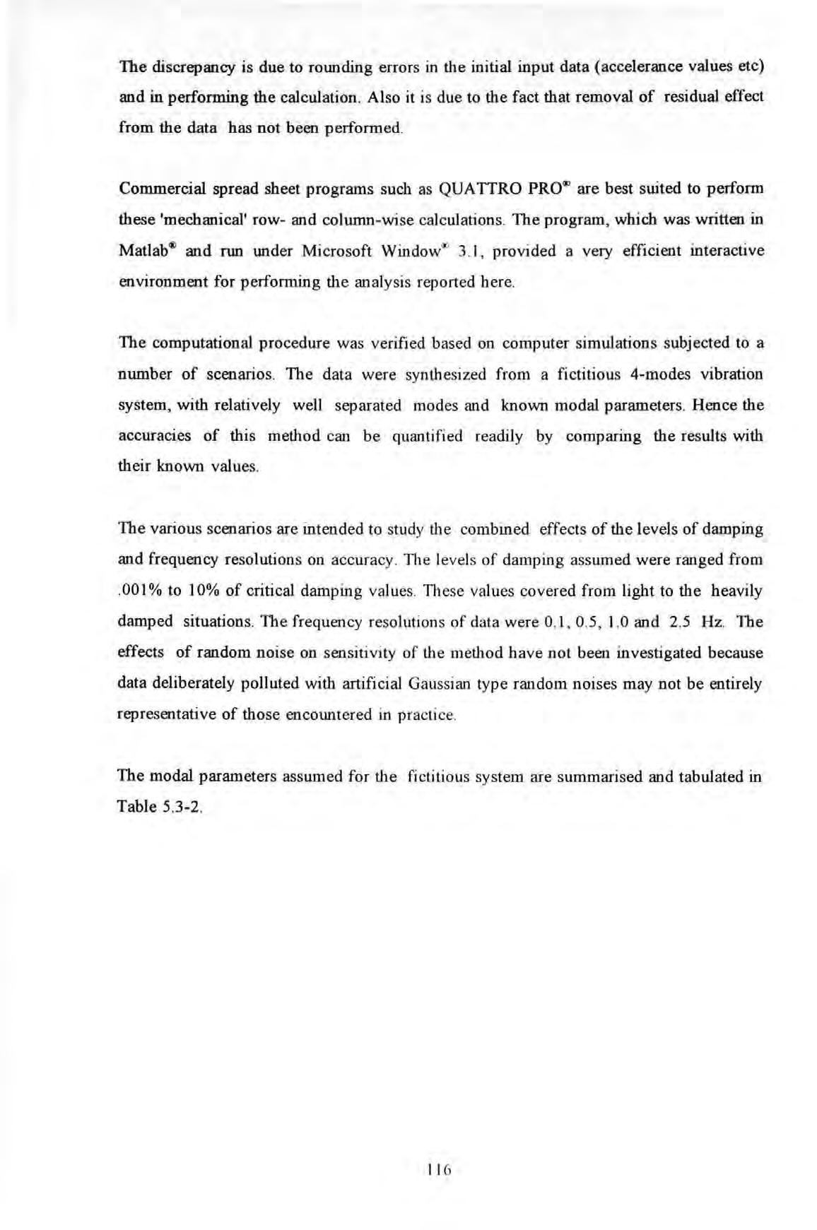
Commercial spread sheet programs such as QUA TIRO PRO® are best suited to perform these 'mechanical' row- and column-wise calculations . The program , which was written in Matlab® and run under Microsoft Window00 3 . 1, provided a very efficient interactive environment for performing the analysi s reported here

The computational procedure was verified based on computer simulations subjected to a number of scenarios. The data were synthesized from a fictitious 4-modes vibration system , with relatively well separated mode s and known modal parameters. Hence the accuracies of this method can be quantified readily by comparing the results with their known values .

The various scenarios are intended to st udy the combined effects of the levels of damping and frequency resolutions on accuracy The levels of damping assumed were ranged from 001% to I 0% of critical damping values TI1ese values covered from light to the heavily damped situations The frequency resolutions of data were 0 1, 0 5 , 1 0 and 2 5 Hz The effects of random noise on sensitivity of the method have not been investigated because data deliberately polluted with artificial Gauss ian type random noises may not be entirely representative of those encountered in practice .

The modal parameters assumed for the fictitious system are summarised and tabulated in Table 5 .3-2 .

In addition to comparing each of the individ ual assumed and determined modal parameters, a statistic called quality-of-fit factor QF is used to indicate q uantitatively how good or bad the overall quality-of-fit or accuracy is . TI1is QF factor has been defined in Section 6 2 3.2 and is subjected to the same limitations in its interpretation as stated there.

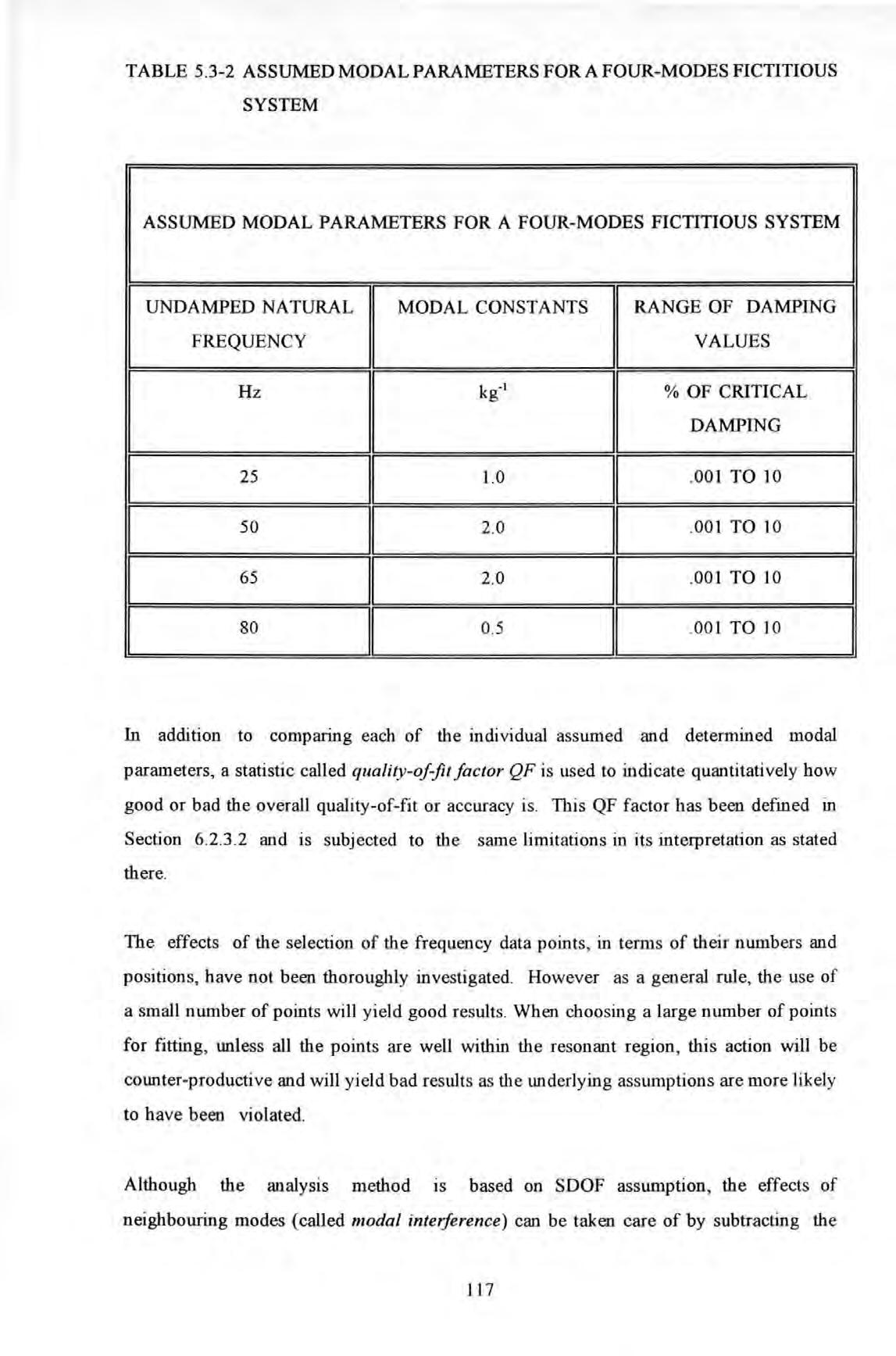
The effects of the selection of the frequency data points, in terms of their numbers and positions , have no t been thoroughly investigated. However as a general rule, the use of a smal l number of points will yield good results When choosing a l arge number of points for fitting , unless all the points are weU within the resonant region, this action will be counter-productive and will yield bad results as the underlying assumptions are more likely to have been violated .

Although the analysis method ts based on SDOF assumption , the effects of neighbouring modes (called m odal interference) can be taken care of by subtracting the effects of these modes from the analyzed mode. Hence accuracy can be further improved by repeating these subtraction procedures in an iterative fashion

The case of 10 % of critical damping has been chosen as an illustration . Although the modal frequencies are relatively well spaced apart, the higher damping level causes considerable 'interference' in the FRF . Analysis conducted using mode s ubtraction on the first three modes has shown some improvements over tho se analysis without using mode subtraction .

For the sake of easy explanation , an indicial notation M(r,s) was devi sed and defined to illustrate the mode subtraction operations carried out as fo ll ows : where r is the mode number s is the number of iterative cycles performed

For instance, M(3 ,2 ) = M(3 , 1) - M(2 , l) means that the results for mode number 3 after two iterations is obtained by s ubtractin g the effects of mode number 2 (from the first iteration) from those of mode number 3 (after the f irst iterations). Table 5 3-2 summarizes the results of analy sis as follows :

TABLE 5 .3-3 RESULTS OF MODAL PARAMETERS DETERMINATION USING ITERATIVE MODE SUBTRACTION FOR THE FOUR-MODE FICTITIOUS SYSTEM

RESULTS OF MODAL PARAMETERS DETERMINATION USING ITERATIVE MODE SUBTRACTION FOR TIIE FOUR-MODE FICTITIO US SYSTEM

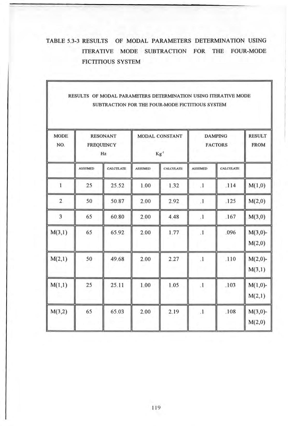
TABLE 5.3-4 EFFECTS ON QF FACTORS BY USING VARIOUS MODE COMBINATIONS

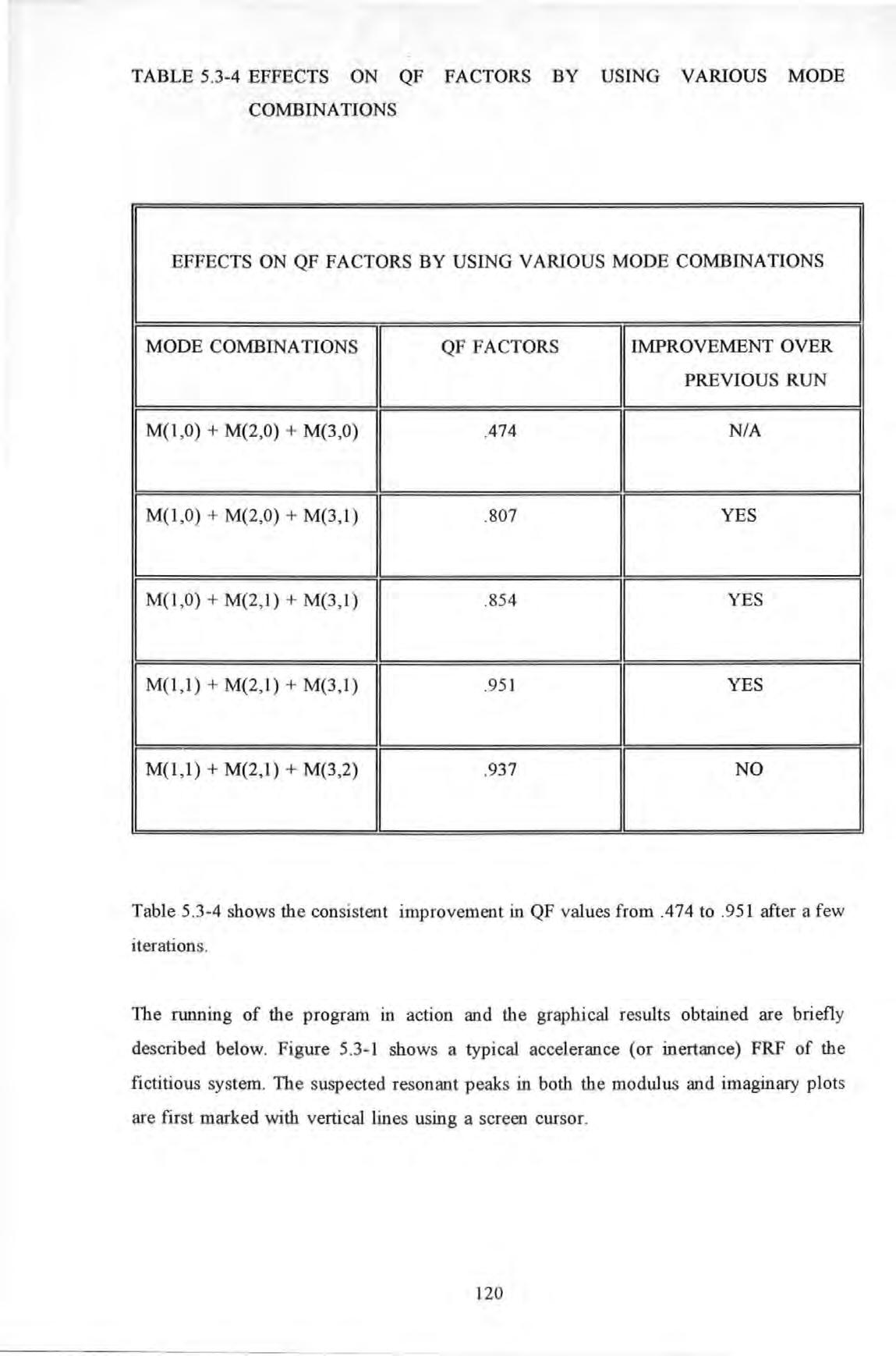
EFFECTS ON QF FACTORS BY USING VARIOUS MODE COMBINATIONS

Table 5.3 shows the consistent improvement in QF values from .474 to .951 after a few iterations .

The running of the program in action and the graphical results obtained are briefly described below. Figure 5.3- 1 shows a typical accelerance (or inertance) FRF of the fictitious system . The suspected resonant peaks in both the modulus and imaginary plots are first marked with vertical lines using a screen cursor.

After responding to a series of requested inputs by the program with regards to : the number of points neighbouring each of the marked peaks used for curve-fitting , whether or not mode subtraction is required, computation then proceeds using the proposed algorithm . To appraise the results obtained, overlaid plots of the original and the so-called regenerated FRF curves are displayed for visual inspection by the analyst. The regenerated FRF curves are plotted based on the determined modal parameters determined (Note the full set of the modal parameters results determined in the simulation experiment are tabulated in Appendix 5.4). A selective sample of these results (plots) for the various conditions studied was shown in Figures 5 .3-2 to 5 .38.

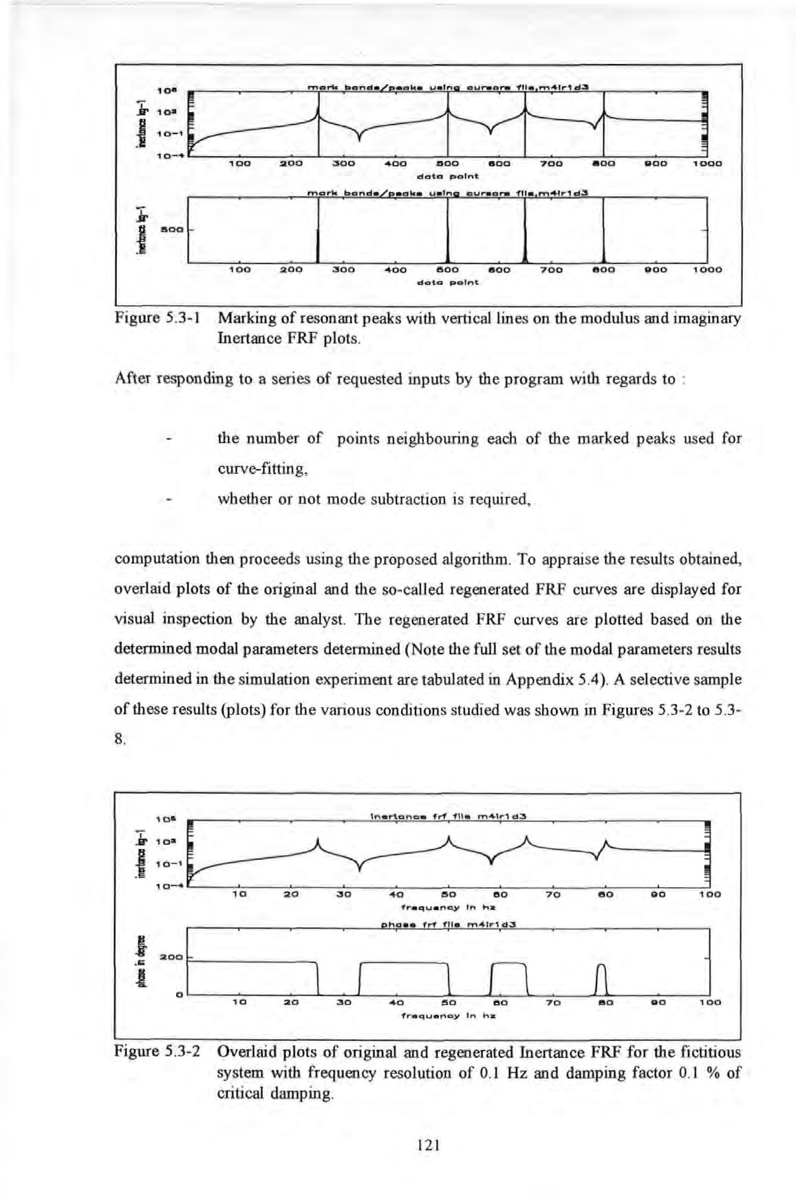
Figure 5 3-2 sho ws that for a frequency resolution of 0 1 Hz and light damping (0 1% of critical damping), the correlation between the two curves in both the modulus and phase plots are very good

Figure

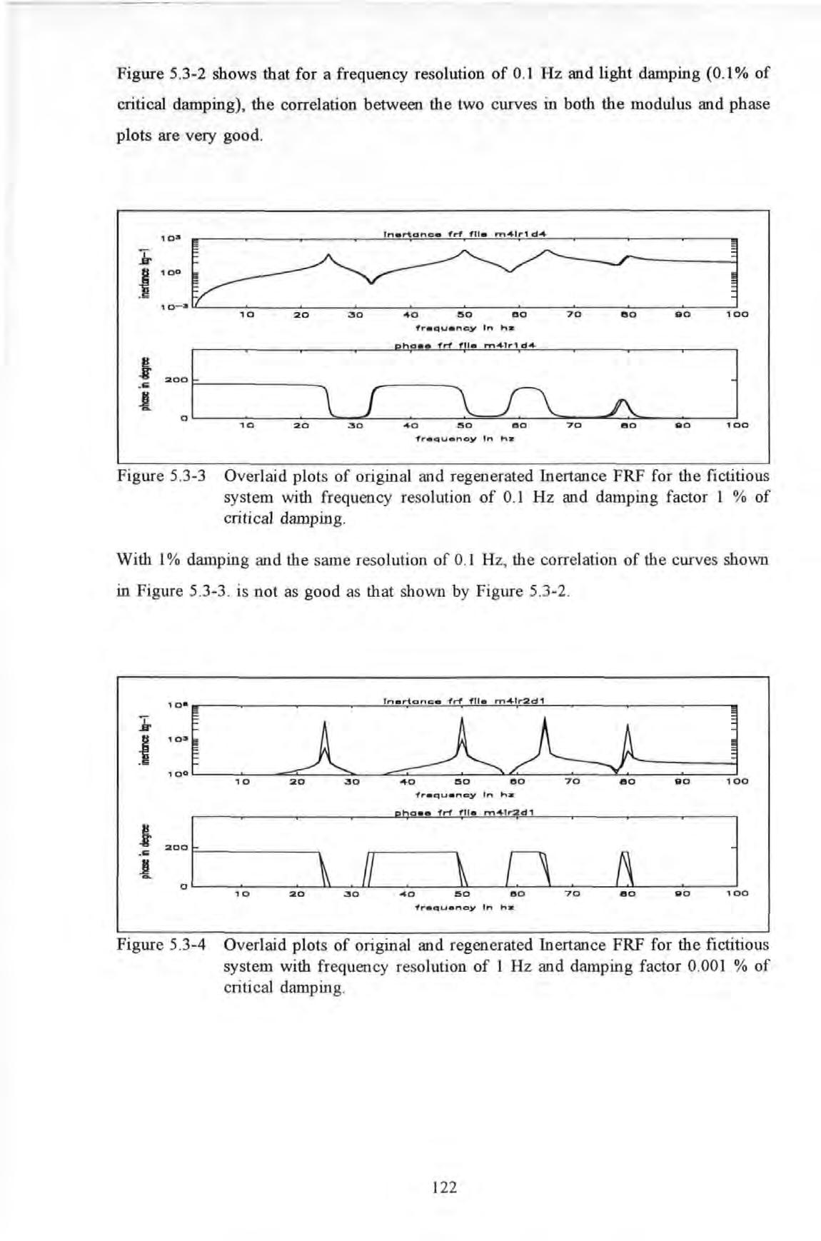
Overlaid plots of original and regenerated Inert.ance FRF for the fictitious system with frequency resolution of 0 . 1 Hz and damping factor 1 % of critical damping

With 1% damping and the same resolution of 0 1 Hz, the correlation of the curves shown in Figure 5 .3-3 . is not as good as that shown by Figure 5 .3-2 .

Figure 5

Overlaid plots of original and regenerated Inertance FRF for the fictitious system with frequency resolution of 1 Hz and damping factor 0.001 % of criti cal damping show that for a frequency resolution of 1 Hz and a range of damping (ranged between .00 I% to O.I% ), correlation is consistently worst at those regions near resonances and anti-resonances where phases change abruptly because of the lack of frequency resolution

% of critical damping.

Figures

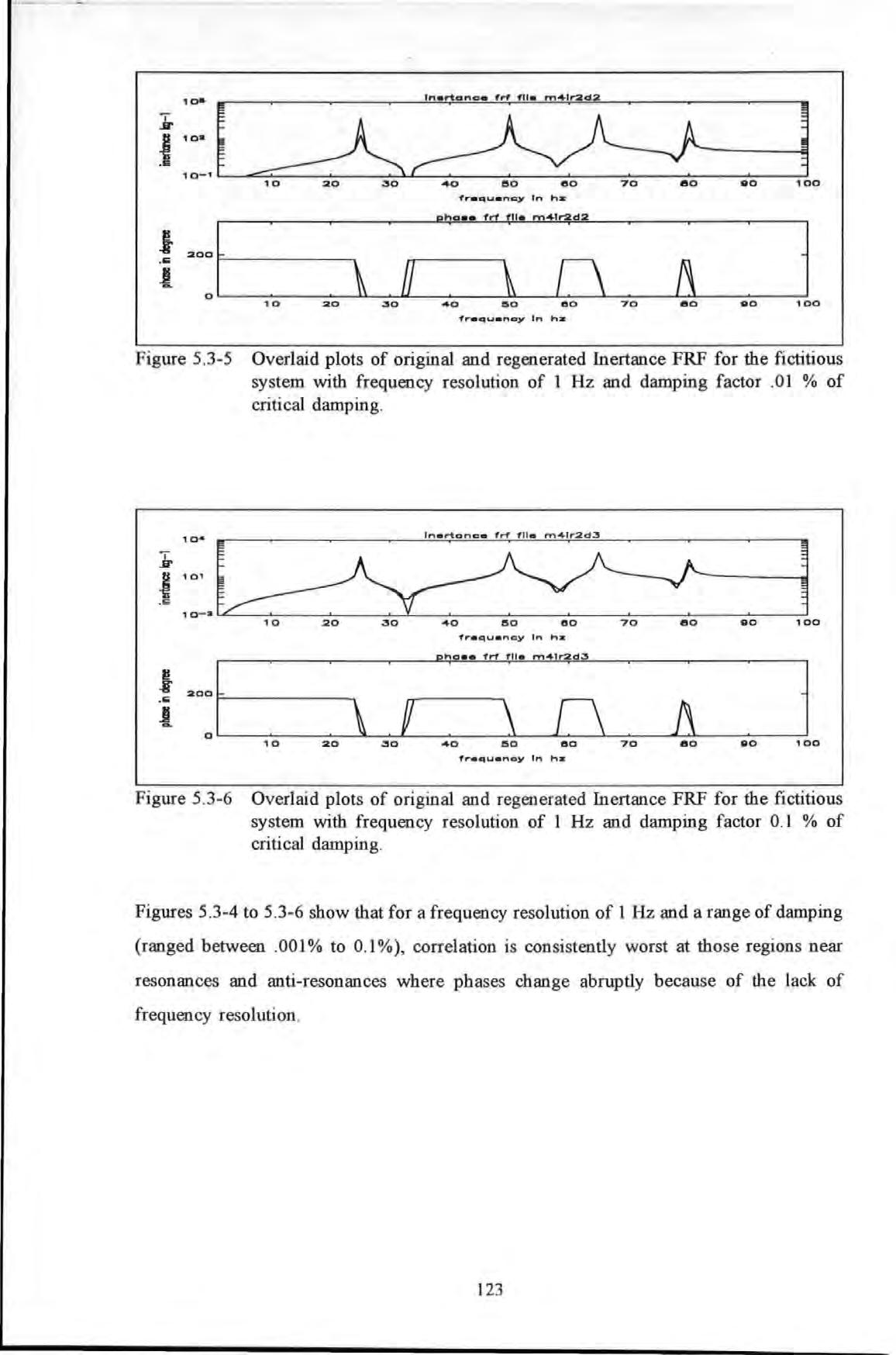
Figure 5 3-7

Overlaid p lots of original and regenerated Inertance FRF fictitious system (with frequency resolution of 2 5 Hz and damping factor 0 001 % of criti cal damping

With a even coarser resolution at 2 .5 Hz, Figure 5.3-7 shows that even with the lightest damping , the correlation deteriorates badly . Results tabulated in Appendix 5.4 show that the errors on the modal parameters set determined are all significantly higher than that of the finer resolution cases given the same damping factors

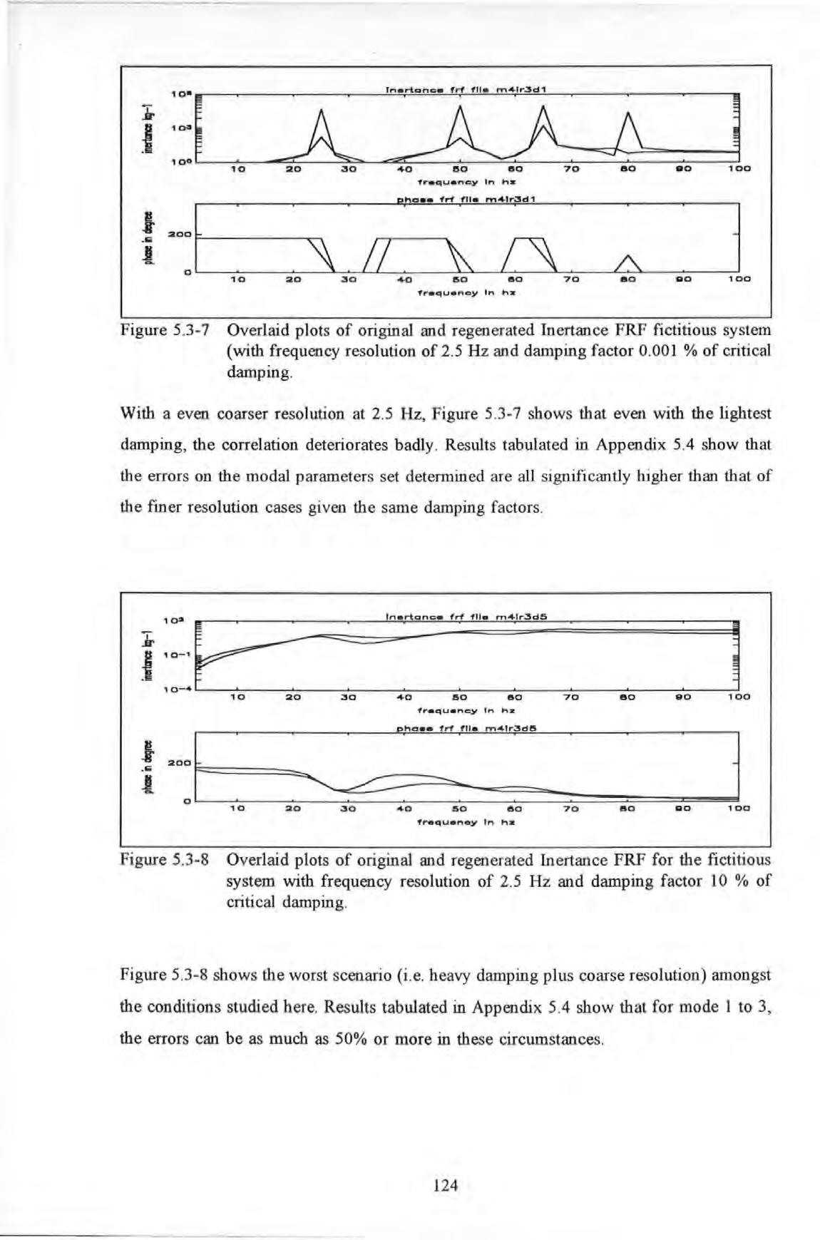
Figure 5 3-8

Overlaid plots of original and regen erated Inertance FRF for the fictitious system with frequency resolution of 2 5 Hz and damping factor 10 % of critical damping

Figure 5 3- 8 shows the worst scenario (i e heavy damping plus coarse resolution) amongst the conditions studied here Results tabulated in Appendi x 5.4 show that for mode 1 to 3, the errors can be as much as 50% or more in these circumstances