CHAPTER 3 THEORY

3.0 INTRODUCTION

Although this project is civil engineering oriented, much of the theories are not nonnally found in civil engineering. So instead of going straight into the theories on experimental modal analysis (introduced in Section 1.2), for the benefits of the readers from the civil engineering background, this chapter is presented under the main theme of mathematical modelling. Under this theme, this research is identified as an experimental modelling approach as a contrast to a theoretical modelling approach such as fmite element method which most civil engineers are familiar with. The bulk of the theories concerning experimental modal or spatial analysis are saved for deliberation in much greater depth later in chapters 5 and 6.

Much of the background theories underpinning this research come mainly from vibration and control engineering. The two disciplines share a lot of common ground. In fact, the mathematical foundations governing systems in control and structural vibration are strikingly similar. Nevertheless, fonnulation of equations and terminology differs a great deal. This chapter is not meant to be an exhaustive account of these theories but only an introduction to the ideas described in the following chapters.

There is no shortage of literature which deals with these theories in great depth. Some literature deal with very fundamental mathematical concepts such as existence and uniqueness of solutions to a fonnulated vibration problem. Others deal with highly complicated theoretical issues such as non-linearity etc. However, few practical engineers would find these theories interesting to read. A simplified approach is therefore presented here.

The concept of mathematical modelling in a wider context is introduced first. The more specific application of modeUing to structural dynamics is then explained. It is considered convenient and conceptually important to describe the conventional theoretical methods under the two categories: continuous (Section 3.2.1) and discrete approaches (Section 3.2.2) applicable to distributive and lumped systems respectively.

The steps leading to the derivation of the governing system equations are described: partial differential equations in the case of a continuous system or a set of linear ordinary differential equations in the case of a lumped system. The methods of solution of these equations are also briefly discussed.

In particular, Eigenvalue solution (Section 3.2.2.2.2), interpretation of Modes of Vibration (Section 3.2.2.2.3) and Orthogonality properties between different modes of vibration (Section 3.2.2.2.4) are introduced in this Chapter. Because these are important theoretical issues which need to be explained and are necessary pre-requisites before deliberating further theories in Chapter 5 and 6. The coverage in these Sections is intended to explain the concept of modal decomposition which forms the whole basis of theoretical and experimental modal analysis. The theories dealing with real modes (associated with undamped or proportionally damped systems) and complex modes (associated with generally or nonproportionally damped systems) are explained in much greater depth in Section 3.2.2.2.5.

The theoretical basis of the experimental approach of modelling, upon which this project is based, is reviewed in Section 3.3. The concept of system identification is introduced in Section 3.3.1 followed by the implementation of this methodology as given in Section 3.3.2. Data measurement and analysis methods are briefly explained in Section 3.3.2.3. Modal methods which derive models in terms of a system's modal parameters are briefly explained in Section 3.3.2.3.1. Non-modal (or spatial) methods which derive models in terms of a system's spatial parameters are also briefly explained in Section 3.3.2.3.2.

3.1 CONCEPTS AND APPROACHES

In essence, the basis of the approach of this investigation can be summarised as an exercise of mathematical modelling. The term mathematical is important here because it distinguishes itself from physical modelling which is the one usually perceived. Physical modelling is a technique based on the Law of Similitude. By studying a reduced scale replica of the original structure, results are then extrapolated to those of the full scale structure. However the latter is not a subject of concern within the scope of this investigation.

3.1.1 MATHEMATICAL MODELLING

Mathematical modelling IS a process m which a complex physical system IS conceptualized and simplified so that it can be expressed in mathematical terms i.e. a series of so called GoverninJ!. Equalions. These equations are equivalent statements of some Laws of Physics, such as the Law of Conservation of Energy and the Newtonian Laws of Motion etc to name a few which are commonly used in the field of mechanics. Having fonnulated the governing equations in an appropriate form, a closed-form analytical solution can often be sought in the case of a simple model or an approximated solution in the case of a complex model, using available analytical or numerical methods.

The derived mathematical representation IS called a model whose major function is to characterize and predict the behaviour of the system studied. A useful model should be one which can make correct prediction in some if not in all situations. Most physical systems in the 'real world' are often too complex for any one model to take into account every single conceivable aspect affecting the system. Important factors have to be correctly chosen and less significant ones be discarded. This process is called conceptual idea/i:::alion. The well established fundamental Laws of Physics which most models are built upon are themselves products of conceptual idealization of nature.

Because idealized assumptions are introduced, the subsequent established model can only be treated as an approximation rather than an exact representation. Mathematical modelling is an art which requires both skill and good judgement rather than sheer manipulations of arithmetic. In most situations, this is carried out iteratively until arriving at an optimal model. This is particularly true for unfamiliar systems whose behaviour is not well understood.

3.1.2 STRUCTURAL MODELLING

Within the scope of structural mechanics, mathematical modelling is an essential and an integral process in analysing structural/mechanical systems: from modelling of behaviours of structural materials, of simple structural elements such as beams and plates to those of complex integral structures in various shapes and forms.

In structural dynamics, structural resonance phenomena can be modelled quite successfully using Eigenvalue theories. Briefly speaking, the natural frequencies and mode shapes of a structure are analogous to the eigenvalues and eigenvectors of the corresponding system equations formulated for the structure (Sections 3.2.2.2.2 will give more details on this). Because mathematical modelling can provide a far-reaching insight into the dynamic characteristics of a structure, even before the structure is built, it is a very useful design and analysis tool.

In essence, the formulated governing equations furnish a relationship between the state of the system (or state variables) and the system parameters. In fluid mechanics, these variables are kinematic quantities such as flow velocity; thermodynamic quantities such as pressure, temperature, enthalpy or entropy. In structural dynamics, the state variables are force (or stress), displacement and its derivatives (or strain/deformation) at a spatial point (or coordinate) of a structure.

The system parameters refer to those quantities, usually constants in the temporal (time) domain, which depend on the geometric, configurational and the constitutive properties of materials of a system. At the microscopic (or material) level, these parameters refer to the Young's modulus, Shear modulus or Lame constants in the case of homogeneous and isotropic structural materials. Whereas at the macroscopic (or structural) level, these parameters are the inertial, stiffness and damping characteristics of an integral structure. It is the method of determining structural parameters (at the structural level) which is the principal concern of this investigation.

Structural models can have varymg degrees of sophistication. In many cases, simple methods are more preferential to use (especially for initial design purposes) than sophisticated ones as the latter often require considerable computational efforts. With the advances of computer technology and methods, models derived from finite elements or boundary elements theories are becoming increasingly popular and sophisticated.

Apart from theoretical means, the advances of computer and instrumentation technology also allow structural modelling to be pursued by experimental means as well.

3.2 THEORETICAL APPROACHES OF MODELLING

The various approaches are explained according to the logical division of continuous and lumped systems. It can be shown that the equations of motion for both systems can be derived using the same set of principles. Among these principles, the Principle of Virtual Work (for static equilibrium cases) can be applied. This principle states: If a system of forces is in equilibrium, the work done by the externally applied forces through virtual displacements (compatible with the constraints of the system) is zero. For dynamic cases, the Virtual Work Principle can be extended to cover dynamic equilibrium using D'Alembert's principle which states that the resultant force must be in equilibrium with the inertia force in a system. Using Variational principle such as the Hamilton's principle, which reduces the problems of dynamics to the investigation of a scalar integral that does not depend on the coordinates system used. The Equations of Motions are obtained from the condition rendering the value of the integral stationary and this is the basis of the Lagrange's Equation.

3.2.1 CONTINUOUS SYSTEMS

A continuous system (or a continuum) is an assemblage of an infinite number of infinitesimally sized particles. All structures, apart from molecular or atomic structures, are continua by nature. By applying the Principles of Equilibrium for each individual particle, the differential equations of motion can be obtained. Alternatively, by integrating these equations within the boundary and domain of a continuum, the integral equations of motion can be obtained. The solution of these differential and integral equations m turn describes the distribution and the gross effects of the state of a system respectively.

A complete theory can be obtained from the mathematical theory of elasticity of solid bodies in general, and elastodynamics in particular. These theories deal with the determination of the state of infinitesimal strain within a solid body which is being subjected to the actions of an equilibrating system of forces. The restriction of infinitesimal strain is important to ensure the validity of linearization of the governing equations to be given below. Nonlinear equations are known to be notorious for presenting difficulties in numerical treatment. Once the equations are linearized, complete solutions can be obtained by superposition of simpler solutions. Other simplified theories based on elementary theory of engineering mechanics are, in fact, derivatives or special cases of these theories. An excellent historical account of the development of the theories of structural modelling is given by Love Jl.tJ

3.2.1.1 FORMULATION OF PROBLEMS

In 1827, Navier derived a set of general governing equations of vibration of elastic bodies based on infinitesimal strain (geo metrical compatibility) and stress (force equilibrium) analyses These equations are now widely known as the Navier Equations which are fundamental to almost all continuum mechanics analysis. Full coverage of this theory is prohibitively long, therefore readers should find the missing details in other standard text books on this subject such as the one written by Love Jl tJ

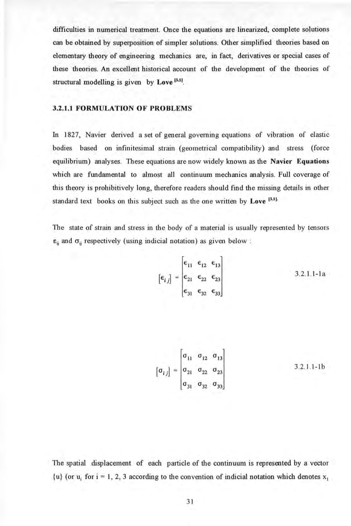
The state of strain and stress in the body of a material is usually repr esented b y tensor s eu and cru respectively (using indicial notation) as given below :

The spatial displacement of each particle of the continuum is represented by a vector {u} (or u; for i = 1, 2 , 3 according to the convention of indicial notation which denotes x 1

, , x3 or x, y, z m the rectangular Cartesian coordinates) and the vanous strain components can be determined by pure consideration of geometry of small deformation .

The stress and strain tensors are both symmetric, where F; p j , j + F; = P * u is the internal body forces is the surface traction or these differential equations can be written in symbolic form as (a 1i ) - P = 0

There are stx independent stress and strain components which occupy the upper triangles of the respective tensors . The condition of the equilibrium of forces m an infinitesimal particle allows the derivation of the equilibrium equations.

(3 2 1.1-4a) (3 2 1.1-4b)

Where is a function of differential operators .

The equations depicted above hold generally regardless of the materials involved However, the relationship between stress and strain is a function of the properties of a material known as the constitutive relations . In mathematical terms, this means that the stress and strain tensors are linked together by fourth order elastic constants tensor cijkl :

Each coefficient cijkl of this tensor is an elastic constant. For isotropic and homogenous materials, these coefficients are functions of only two independent material constants called the Lame constants It can also be shown that the usual material constants : the Young's modulus E and Shear modulus G , can be expressed in terms of the two Lame constants A. and ll · Using indicia] notation , this relationship can be written as :

2 1 1-6)

In the absence of internal body forces F; , the following Navier's equations can be obtained :

.2 . 1.1-7) where p is mass density of material and A , Y' 2 are given in extenso : called the dilatation

A = au 1 at.

+ called the Laplacian Operator

After some manipulations , these equations can be reduced to the well known Wave Equations which describe the propagation of dilatational and shear waves in solids or the vibratory motions in an elastic continuum . Detail discussions on this subject are given by Clark ll.JI _

A closed-form solution can only be obtained if the compatibility (or integrability) requirements are also satisfied in addition to the equilibrium and constitutive requirements .

This is because the condition of a stress distribution in equilibrium with the given imposed loads does not necessarily imp ly a compatible strain fiel d and VICe versa. The compatibility equations are given below:

Equation (3 2.1.1-7) formulates the problem entirely in terms of displacements u;. The true solution would also require u; to satisfy the prescribed boundary disp lacement condition as well However since the problem is posed entirely in terms of displacements, compatibility Equation {3 .2. 1.1 - 8) will be satisfied automatically.

3.2.1.2 METHODS OF SOLUTION

Having derived the partial differential governing equations, it remains to find a solution when traction and disp lacements on the boundary of a continuum are prescribed.

Under suitable conditions, a unique closed-form solution depicting the stress and strain state of each particle can be determined .

There are a variety of methods available to solve these equations : series, singularities, difference, collocation and variational methods to name a few . However it is beyond the scope of this thesis to fully explain these methods. Further details can be found in Love 13"11 and Ricbards 13•41·

3.2.2 DISCRETE OR LUMPED SYSTEMS

A closed-form solution to the governing differential equations shown in Section 3 .2. 1 can be very difficult to obtain except for simple cases only An alternative approach can be applied using approximations This approach performs a conceptual subdivision of the continuous domain into discrete elements of simpler forms . This process 1s often known as discretization There are two different techniques available in this respect i e a domain discretization method typified by Finite Element Methods (FEM) and a boundary discretization method typified by Boundary Element Methods (BEM). In domain methods , the governing equations of the problem are approximated over the region by functions which fully , or partially, satisfy the boundary conditions However in boundary methods, approximating functions are used which satisfy the domain but not the boundary conditions Though BEM are claimed to have certain advantages over FEM in some ways , such as : a. a smaller problem size in term of data storage and computation , b . more efficient in handling problems with an infinite domain or small surface to volume ratio and c . quicker to converge to a solution etc,

FEM are more popular with many commercial software available such as PAFEC , NASTRAN and ANSYS etc In contrast, very few commercial BEM software are availabl e

3.2.2.1 FORMULATION OF PROBLEM

FEM and BEM can be derived from the Weighted Residual, Variational or Functional principles Furthermore, it can be shown that the Weighted-Residue theory can provide a unified description of both methods (see Brebbia ) The Weighted-Residual methods are numerical procedures for approximating the true solution Uo of a set of differential equations of the form :

( uJ = P in 0 where 0 is the domain when subjected to the following boundary conditions : essential boundary conditions G(uo) = g (on r 1) and natural boundary conditions S(uo) = q (on r :J where rl and r 2 is the total boundary

3.2.2.1-1

3.2.2.1-2

The approximate solution u of the true solution u0 I S approximated by a set of functi on s Yk(x) such as :

N u = L at iix) A:=l where i 1(x), i 2 (x) .... iix) .... iJ..x) are a set of linear independent fimctions and a l' a 2 at """ aN are a set of undetermined parameters

3.2.2.1-3

The residual error is defined as the error function t as depicted in the following equation e = (u) - P * 0

3 2.2. 1-4

This residual error is generally non-zero except in the case of an exact solution However thjs can be forced to zero in an average sense by a weighted integral of the

Convergence towards the exact solution is achieved as the number of terms increase. A variety of methods are available: the Galerkin's and the Rayleigh-Ritz methods to mention a few. However, a unified description of these methods can be obtained using the ideas of weighting functions w In its simplest description , the governing equation 3 2 2 1-1 can be re-written by the introduction of weighting functions :

where w is the weighting functions .

It can be shown that methods such as Galerkin's, Rayleigh's and Virtual Work only differ in the ways in which the weighting function s are cho s en . In the case of Galerkin's method , the weighting functions are chosen in the same way as the trial functions

Equation 3 .2 .2 . 1-8 produce a system of equations from which the unknown parameters ak can be solved

3.2.2.2 SOLUTION USING FINITE ELEMENT METHODS

In essence, the analysis of an integral structure is broken down into one of an assemb lage of a large number of elements (called finite elements) which are of various shapes and sizes. Most structures can be idealized as an assemblage of b eams, membranes , plates etc. The results of discretization are manyfold. Firstly, a structure is replaced conceptually by elements forming a mesh : the lin es occur where element boundari es come together and the nodes where the element corners meet. Secondly , the governing equation s of the continuum are replaced by a set of simultaneous algebraic linear equations . Further theories on FEM can be found in some authoritative text books such as those written by Robinson 13 • 6 1 and Zienkiewicz 13 7 1

3.2.2.2.1 CONSTRUCTION OF STRUCTURAL MATRICES

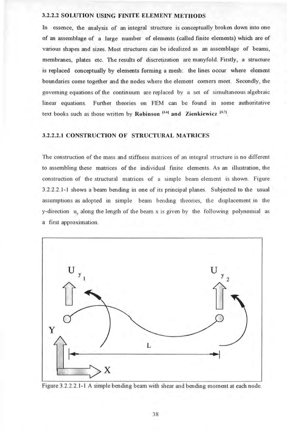
The construction of the mass and stiffness matri ces of an integral structure is no different to assembling these matrices of the individual finite elements As an illustration , the con s truction of the structural matrices of a s impl e beam element i s shown. Figure where the a's are arbitrary constants. If expressed in matrix notation : where {a} IS a vector of the constants a's and [POLY] is a polynomial matrix :

3 2 2 2 1-1 shows a beam bending in one of its principal planes Subjected to the usual assumption s as adopted in simpl e beam bending theories, th e displacement in the y-direction lly along the length of the beam x i s given by the following polynomial as a first approximation .

The constants a's can be solved if the nodal displacement boundary conditions are known . The choice of a 3'd order polynomial now becomes apparent since the four pieces of information on the nodal displacement enable the constants a 1, a3 and a4 to be solved . This relationship can be expressed in matrix form :

Therefore the displacement of any intermediate point between the nodal points can be interpolated using : when expanded :

The strain energy S.E. associated with such beam deformation is given by : where

As by definition, the S .E. can also be expressed as :

In 3D analysis , a beam can be subjected to twist and axial deformations when under the action of couples and axial forces . As these deformations do not affect those due to flexure , the effects are combined together using superposition The axial and torsional displacements of any one point between the nodal points can be approximated by including the axial u,.(x) and torsional q(x) displacement fields :

Then the steps described previously can be repeated to determine the full stiffness matrix taking into account axial, bending, shear and torsion. This matrix is too large to be presented here and only the stiffness matrix due to shear and bending of a beam is given here:

Similarly , the mass matrix derived is based on Kinetic Energy considerations. The kinetic energy K.E of a beam with the aforementioned deformations is given by : where ro is the angular frequency of oscillation

Also by definition, the K.E. can also be expressed as :

Therefore the mass matrix can be obtained by using :

Although the derivation process of a relatively simple beam element is shown , other elements such as membrane and plate bending elements etc. can also be obtained by following these procedures : a To make an assumption of the displacement fields which are appropriate to the element's geometry and proposed structural actions. These displacement fields are expressed in the form of polynomials and in terms of some arbitrary constants . b To write the expression of the strain energy in terms of displacements by making use of interpolation to determine the displacements of any point within the element from the nodal displacements.

Having obtained the elemental structural matrices of each individual element, the global structural matrices can be obtained by assembling the individual elemental matrix. The end product of these operations is a set of linear algebraic equations ready for solution. So far, the theoretical development covers a free undamped system and these equations are usually stated as : where {x} is a vector of nodal displacement

According to the coordinate system , the scheme of numbering of elements and nodes used , [M] and [K] are not usually diagonal matrices ([M] may be diagonal if lumped mass model is assumed) . In this case, the system of equations are coupled. Decoupling of the equations is achieved (to be proved later in Section 3 2.2.2 4) through linear transformation of the arbitrary coordinate system {x} to natural coordinates {ll} using the classical undamped modal matrix [<I>] (as illustrated in Equation 3.2.2.2 . 1-19):

3.2.2.2 . 1-1 9 (x} = [4>] *{ TJ}

Note that the coordinate transformation does not change the character of the system, it simply facilitates solution Pre-multiplying Equation 3 .2.2 2 .1 - 18 by [<I>]T and with the substitution of Equation 3.2 .2. 2 1-1 9, Equation 3 2.2 2.1-20 is obtained:

* ( ii } + [4>f[K]4>] * ( , } = ( 0 } 3 .2.2 .2. 1-20

Denoting :

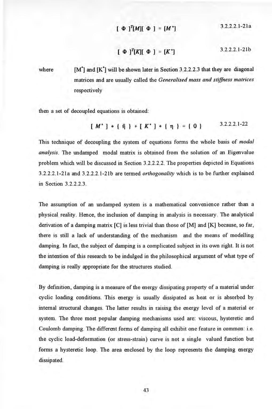
[M*] and [K*] will be shown later in Section 3 2 2 2 3 that they are diagonal matrices and are usually called the Generalised mass and stiffness matrices respectively then a set of decoupled equations is obtained:

This technique of decoupling the system of equations forms the whole basis of modal analysis. The undamped modal matrix is obtained from the solution of an Eigenvalue problem which will be discussed in Section 3.2.2.2.2. The properties depicted in Equations

3 2 2.2 1-21a and 3 2.2 2 1-21b are termed orthogona/ity which is to be further explained in Section 3 .2.2 .2.3 .

The assumption of an undamped system is a mathematical convenience rather than a physical reality . Hence, the inclusion of damping in analysis is necessary . The analytical derivation of a damping matrix [C] is less trivial than those of [M] and [K] because, so far , there is still a lack of understanding of the mechanism and the means of modelling damping In fact , the subject of damping is a complicated subject in its own right. It is not the intention of this research to be indulged in the philosophical argument of what type of damping is really appropriate for the structures studied .

By definition , damping is a measure of the energy dissipating property of a material under cyclic loading conditions This energy is usually dissipated as heat or is absorbed by internal structural changes . The latter results in raising the energy level of a material or system. The three most popular damping mechanisms used are : viscous , hysteretic and Coulomb damping The different forms of damping all exhibit one feature in common : i e the cyclic load-deformation (or stress-strain) curve is not a single valued function but forms a hysteretic loop . The area enclosed by the loop represents the damping energy dissipated.

Linear viscous damping prop erty is characterised by a dashpot Viscous damping force acts in a direction opposite to the direction of and with amplitude proportional to the amplitude of velocity of a coordinate. Viscous damping force is also frequency dependent. Hysteretic damping is associated with internal energy loss due to material hysteresis Hysteretic damping force acts in a direction opposite to the velocity of and with amplitude proportional to the amplitude of displacement of a coordinate. Coulomb damping is attributed from the energy loss by friction at an interface or joint between mating members where relative mechanical motion occurs Coulomb damping force acts in a direction opposite to the velocity of a coordinate and with constant amplitude It is independent of amp litud e of displacement and velocity of a coordinate. Both hysteretic and coulomb damping forces are frequency independent.

The choice of a suitable damping model is not usually an exact science and is often a matter of preference or convenience Viscous damping is widely used especial ly in the civil engineering community . However, some people show special preference to hysteretic damping because of the expedience it can offer in simplifying some complicated mathematical expressions.

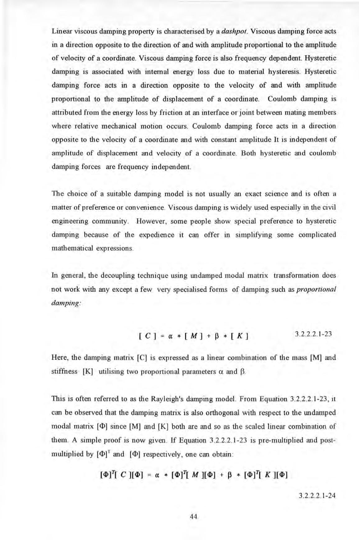
In general, the decoupling technique using undamped modal matri x transformation does not work with any except a few very specialised forms of damping such as proportional damping :

Here, the damping matrix [C] is expressed as a linear combination of the mass [M] and stiffnes s [K] utili s in g two proportional parameters ex. and

This is often referred to as the Rayleigh's damping model. From Equation 3 2 2 2 1-23 , it can be observed that the damping matrix is also orthogonal with respect to the undamped modal matrix [<l>] sin.ce [M] and [K] both are and so as the s caled linear combination of them . A simple proof is now given . If Equation 3 .2 .2 .2 . 1- 23 is pre-multiplied and postmultiplied by [<I>t and [<l>] respectively , one can obtain :

Mter some appropriate substitutions, one can obtain : where [C•] is a diagonal matrix similar to [M•] and [K.], and 1s called the Generalised Damping matrix

Hence the proof is completed From Equation 3 2.2 2.1-26 , one can obtain a relationship which enables the two Rayleigh' s constants a and J3 to be determined if values of modal damping factor and undamped natural frequency ro. are known

If experimental data on the modal damping factors is available, the damping matrix [C) can be constructed using (which is a diagonal matrix of the modal damping factors of the various modes of vibration), the analytically determined spectral matrix and the undamped modal matrix (i e they are obtained after solving an eigenvalue problem associated with the corresponding undamped system) : is the undamped modal matrix is the diagonal matrix of modal damping factors is the diagonal spectral matrix

So with the inclusion of damping, the fully assembled equation of motion for a damped system under forced vibration is : is the forcing vector

The stzes of the structural matrices [M], [C) and [K] depend on the number of degrees of freedom required to specify the deformation fiel d. They can be very large even for a structure of modest size and complexity. Hence a process known as condensation (static or dynamic condensation) is often applied to reduce the size of these matrices before carrying out a computer solution. In essence, the original matrices are condensed by only retaining the master degrees of freedom and eliminating all the unwanted slave degrees offreedom in the equations It can be shown that in the case of static or dynamic condensation, the condensed stiffness matrix is exact, but the condensed mass matrix is not but an approximation only

A complete solution of the eigenvalue problem of large matrix size can involve very intensive computation However, if only a small number of the lower natural frequencies and mode shapes of a system is required , there are a few computational schemes available which do not require a complete solution

3.2.2.2.2 EIGENVALUE SOLUTIONS

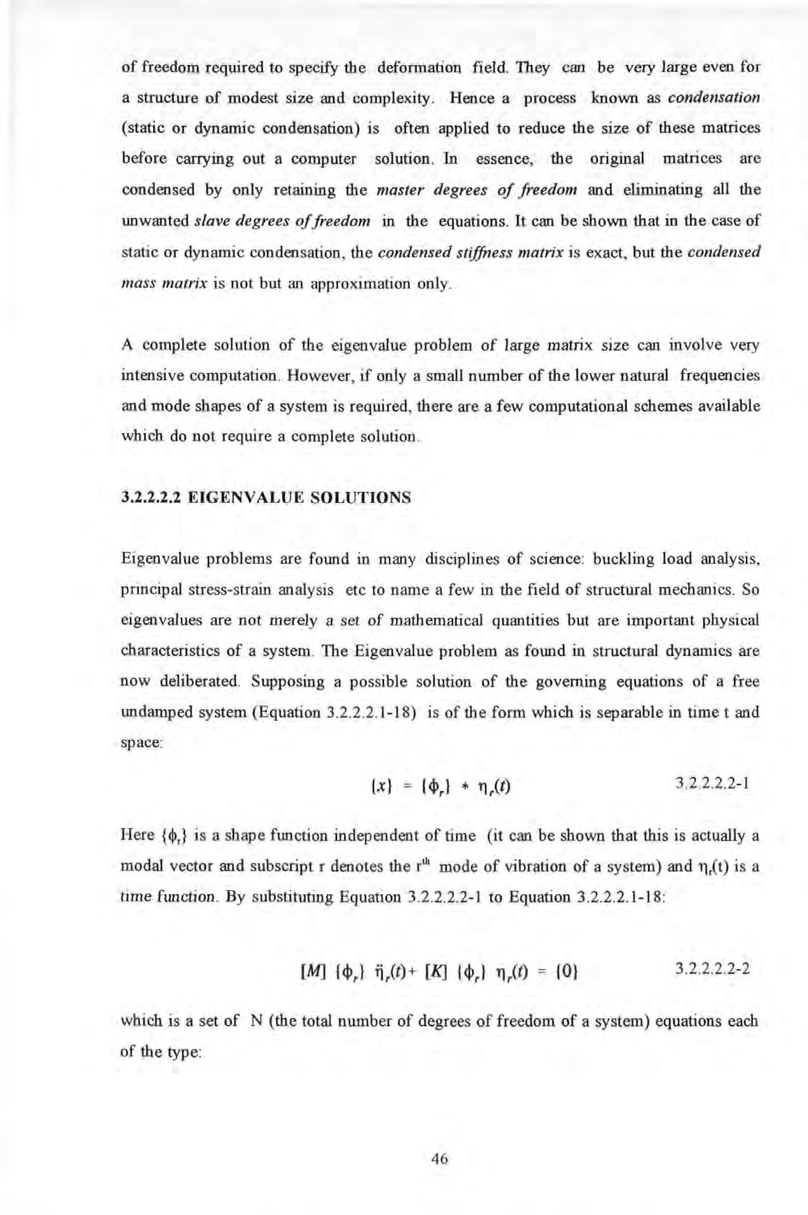
Eigenval ue problems are found in many disciplines of science : buckling load analysis, principal stress-strain analysis etc to name a few in the field of structural mechanics So eigenvalues are not merely a set of mathematical quantities but are important physical characteristics of a system. The Eigenvalu e problem as found in structural dynamics are now deliberated Supposing a possible solution of the governing equations of a free undamped system (Equation 3 .2 .2.2.1-18) is of the form which is separable in timet and space:

Here {cl>,} is a shape function independent of time (it can be shown that this is actually a modal vector and subscript r denotes the rw mode of vibration of a system) and 11.Ct) is a time function By substituting Equation 3.2.2.2.2-1 to Equation 3 2.2 2 1-18 : 3 .2 .2.2.2-2 which is a set of N (the total number of degrees of freedom of a system) equations each of the type :

Using the method of separation of variables,

The positive sign is chosen for a conservative system. Hence two sets of equations are obtained :

The solution to Equation 3.2 2 2 2-5 is of the form : where the amplitude c. and phase angle <p. are determined by the initial conditions. This solution stipulates that all the coordinates perform a harmonic motion with identical frequency ror and identical phase angle <p• The values of these frequency ro. are governed by the Equation 3 2.2.2.2-6 which can be recast in matrix form as: which is the standard formulation for a special mathematical problem called Eigenva/ue problem A trivial solution to Equation 3 2.2.2 2-8 is {cilr} which is equal to a zero vector. Such a solution represents the static equilibrium case Non-trivial solutions exist if the characteristic equation (Equation 3.2 2 2 2-9) is satisfied where A cd is called the characteristic detenninant.

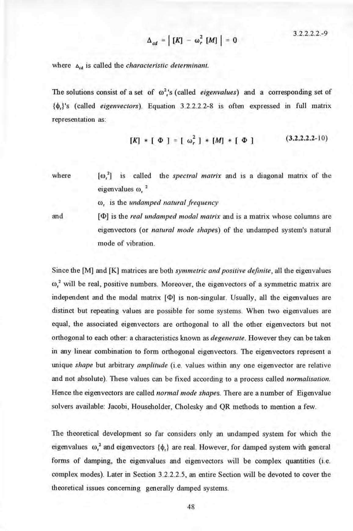
The solutions consist of a set of ro 2.'s (called eigenva lu es) and a corresponding set of {<jl,}'s (called eigenvectors) . Equation 3 .2 .2 .2 .2-8 is often expressed in full matrix representation as :

[ro,2 ] 1s called the spectral matrix and 1s a diagonal matrix of the eigenvalues ro, 2 m, is the undamped natural frequency

[<l>] is the real undamped modal matrix and is a matrix whose columns are eigenvectors (or natural mode shapes) of the undamped system's natural mode of vibration .

Since the [M] and [K ] matrices are both symmetric and positive definite , al l the eigenvalues ro, 2 will be real , positive numbers. Moreover, the eigenvectors of a symmetric matrix are in d ependent and the modal matrix [<l>] is non-singular Usually, all the eigenvalues are distinct but repeating values are possible for some systems When two eigenvalues are equal, the associated eigenvectors are ortbogonal to all the other eigenvectors but not orthogonal to each other: a characteristics known as degenerate However they can be taken in any linear combination to form ortbogonal eigenvectors The eigenvectors represent a unique shape but arbitrary amplitude (i.e values within any one eigenvector are relative and not absolute) These values can be fixed according to a process called nonna/isation. Hence the eigenvectors are called nonna/ mode shapes . There are a number of Eigenvalue solvers available : Jacobi , Householder, Cholesky and QR methods to mention a few

The theoretical development so far considers only an undamped system for which the eigenvalues m/ and eigenvectors {<!J,} are real However, for damped system with general forms of damping, the eigenvalues and eigenvectors will be comp lex quantities (i e complex modes) Later in Section 3 2 2 2 5, an entire Section will be devoted to cover the theoretical issues concerning genera lly d amped systems.