5.4 COMPARISON OF THE PROPOSED WITH SOME CONVENTIONAL METHODS

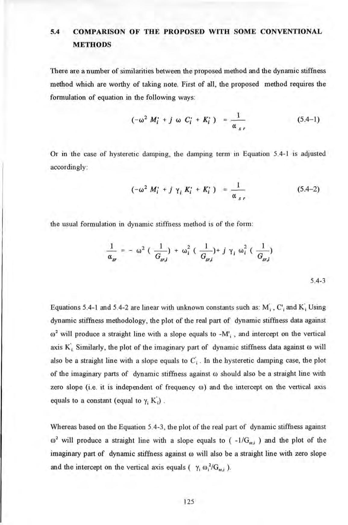
There are a number of similarities between the proposed method and the dynamic stiffness method which are worthy of taking note First of all , the proposed method requires the formulation of equation in the following ways : 1 (5.4-1) as r

Or in the case of h ysteretic damping , the damping term m Equation 5.4-1 is adjusted according}y : 1 (5.4- 2) as r the usual formulation in dynamic stiffness method is of the form :

Equation s 5.4-1 and 5.4-2 are linear with unknown constants s uch as : M';, C'; and K'; Using dynamic stiffness methodology , the plot of the real part of dynamic stiffness data against ro 2 will produce a straight lin e with a slope equals to - M '; , and intercept on the vertical axis K'i. Similarly, the plot of the imaginary part of dynamic stiffness data against ro will also be a straight line with a s lope equals to c'; . In the hysteretic damping case, the plot of the imaginary parts of dynamic stiffness against ro should also be a straight line with zero slope (i.e. it is independent of frequency ro) and the intercept on the vertical axis equals to a constant (equal to Y; K ';) .

Whereas based on the Eq uation 5.4-3, the plot of the real part of dynamic stiffness against ro 2 will produce a straight line with a slope equals to ( - 1/G,,.; ) and the plot of the imaginary part of dynamic stiffness against ro will also be a straight line with zero slope and the intercept on th e vertical axis equals ( Y ; ro; 2/G.,,; ) .

Secondly, both the proposed method and the dynamic stiffness method require the removal of the residual effect of out-of-range modes from the raw data as a separate and a prerequisite step for an accurate analysis. Thirdly, both the proposed method and the dynamic stiffness method assume real modes hence they all implicitly assume proportional damping.

However, despite these similarities, the two approaches do differ in· the fundamental thinking. The proposed method here determine the spatial parameters M; , K"; and c·; (called effective mass, damping and stiffness) directly. This approach is in line with the philosophy as will be discussed in Chapter 6. From these spatial parameters, the modal parameters are then derived as 'by-products'. Whereas the dynamic stiffness method determines the modal parameters directly. Unlike modal parameters, these spatial parameters still retain some quantitative descriptions of mass, stiffness and damping of a system.

A comparison of the proposed algorithm with two other SDOF methods (i.e. the circleand Dobson's improved straight-line-fit methods) was carried out. Again the same 4-modes fictitious system was used for this study. It was expected that the proposed method would achieve similar accuracy as the corresponding dynamic stiffness method would if the residual-removal step was carried out as a pre-requisite step before fitting,. The intention of this comparison study was to determine the accuracy of the proposed method in the event that the residual-removal step was not carried out. The areas of comparison were also concentrated on the effects of different levels of damping, frequency resolutions and fitting data points selections on accuracy. The results obtained from the three methods carried out are tabulated in Appendix 5.4 but some general observations are summarised below.

In general the circle-fit method is not suitable for very light damping cases and can produce large errors if frequency resolution is not fme enough. In the heavy damping situations, this method has yielded results with better accuracy.

The Dobson method has a good overall performance in many situations due to the elaborate procedures included in the program: a. to subtract or minimize the effects of modal'interference' from neighbouring modes on the analyzed mode. b. to account for complex residual effects from out-of-range modes.

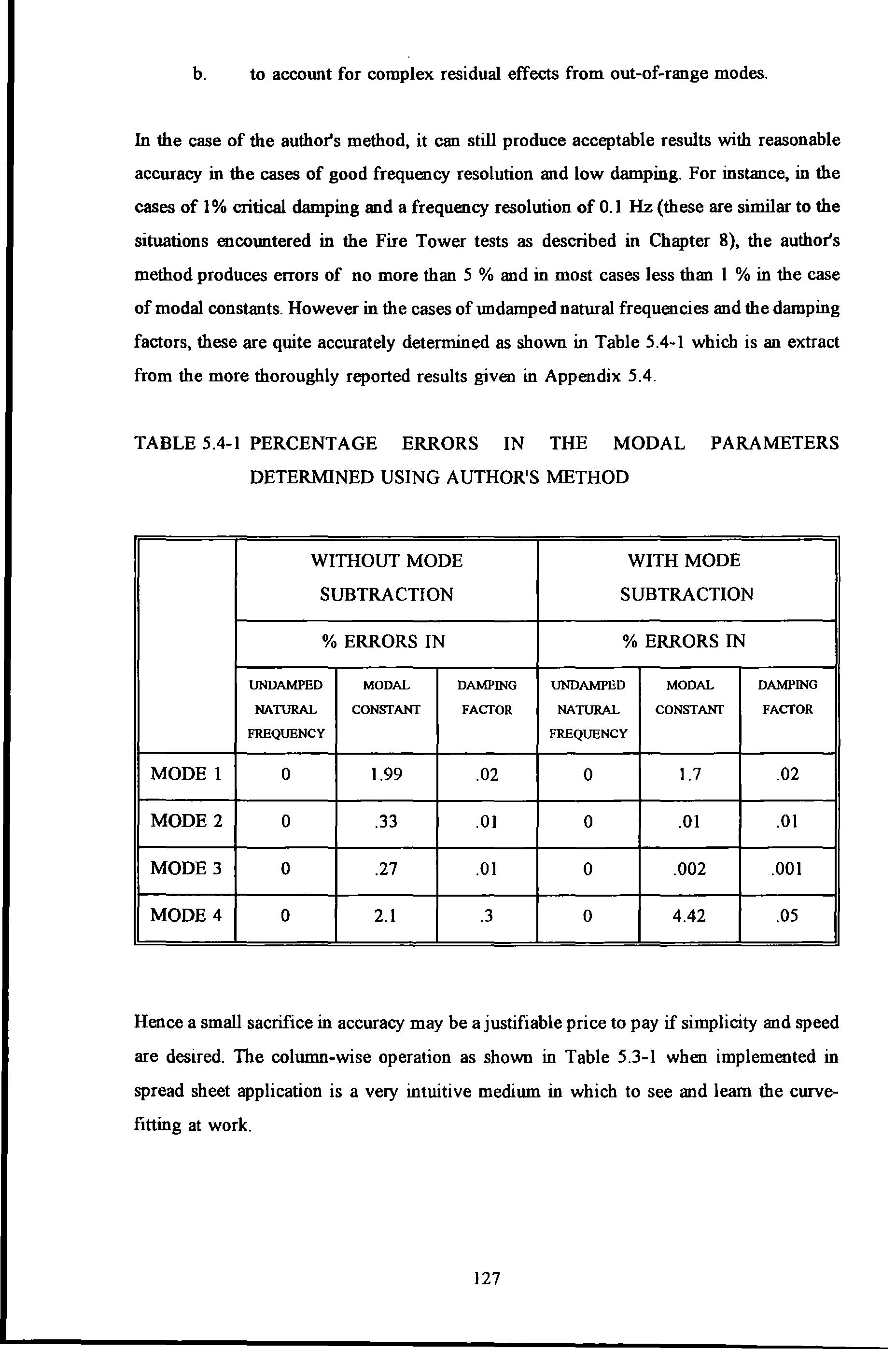
In the case of the author's method, it can still produce acceptable results with reasonable accuracy in the cases of good frequency resolution and low damping. For instance, in the cases of 1% critical damping and a frequency resolution of 0.1 Hz (these are similar to the situations encountered in the Fire Tower tests as described in Chapter 8), the author's method produces errors of no more than 5 % and in most cases less than I % in the case of modal constants. However in the cases of undamped natural frequencies and the damping factors, these are quite accurately determined as shown in Table 5.4-l which is an extract from the more thoroughly reported results given in Appendix 5.4.

TABLE 5.4-l PERCENTAGE ERRORS IN THE MODAL PARAMETERS DETERMINED USING AUTHOR'S METHOD

Hence a small sacrifice in accuracy may be a justifiable price to pay if simplicity and speed are desired. The column-wise operation as shown in Table 5.3-1 when implemented in spread sheet application is a very intuitive medium in which to see and learn the curvefitting at work.