3.3.2.1 EXPERIMENTATION

Data acquisition is often used synonymously with experimentation or instrumentation. Recent advances in instrumentation and computer technologies have brought about great changes in the various aspects of experimentation when compared to those one or two deca des ago . The specific details of the instrumentation requirements will be dealt with in Chapter 4 .

The basics of the experimentation involves the application of some forms of excitation to and the measurement of the s ubsequent responses of a structure. The number of excitation inputs and the way they are app lied can affect the subsequent analysi s procedures A variety of methods are available : from Single-Input- Single-Output (SISO) , Single-Input-Multiple-Output (SIMO), Multiple-Input-Single-Output (MISO) to MultipleInput -Multiple-Output (MIMO) methods etc. Normal mode testing is an example of the techniques using multiple exciters . The amp litudes and phases of the mono-frequency force vector, generated s imultaneously by an array of exciters, are carefully adjusted (or apportioned) until a so-called mono -phased response vector is obtained . The adjustment is required to produce a force vector to b alance out the damping force vector.

Multiple excitations are generally difficult to implement in field testings because of the high equipment co sts of exciters and operati onal restrictions imposed in the field. Among the methods avai lab le, this study has adopted the SISO method which is, by far, the easiest to implement. This method requires only one single excitation input and only response at on e test point of a structure needs measuring at any one time The SISO test procedures are simply repeated to cover the rest of the structure.

3.3.2.2 FREQUENCY RESPONSE FUNCTION MEASUREMENTS

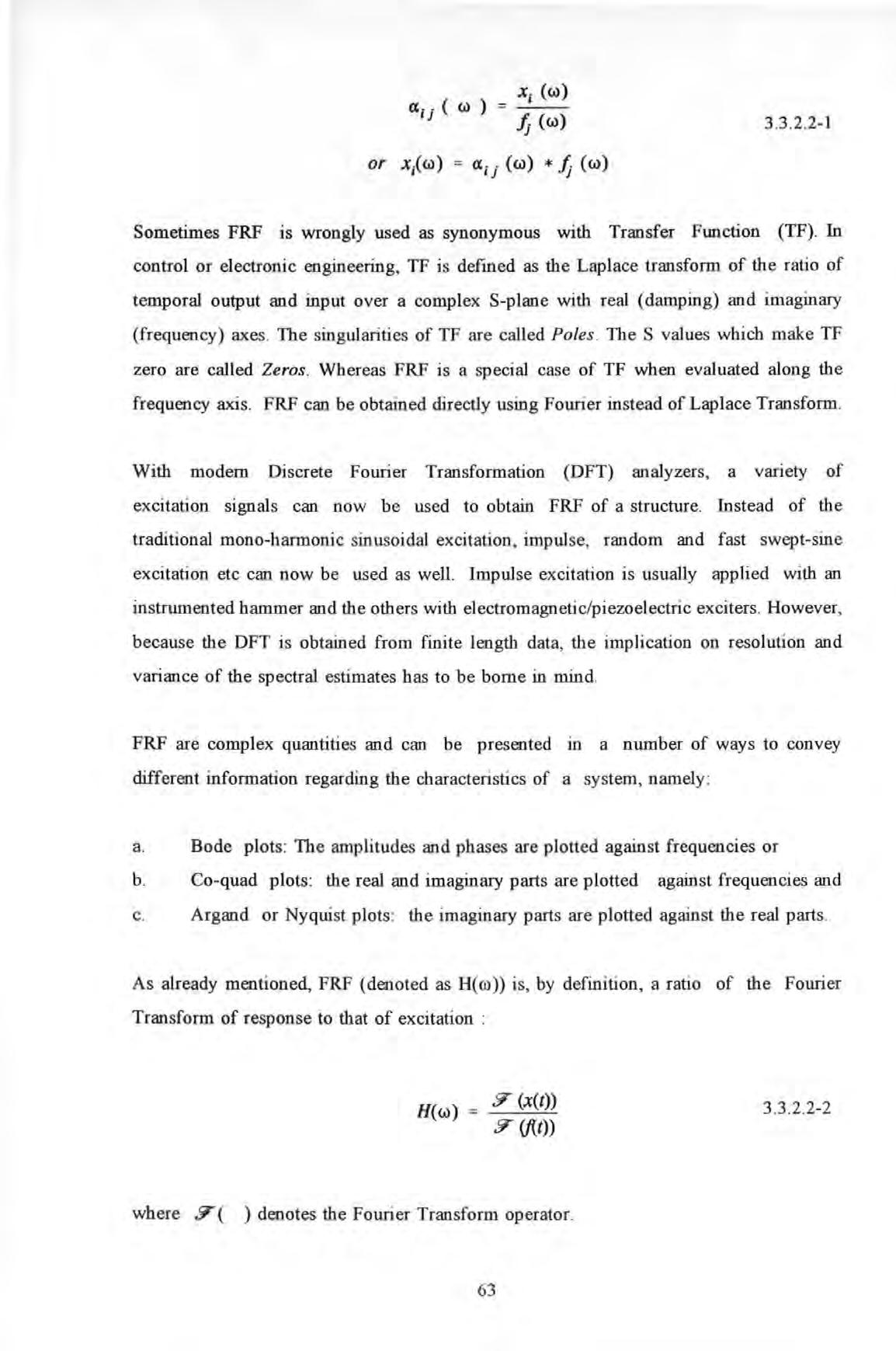
The experimental data acquired are in the form of Frequency Response Function (FRF) measurements FRF , as traditionally used in el ectronic engineering, refers to the amplitude ratio and phase difference between the sinusoidal voltage output and sinusoidal voltage input to a circuit (system). In structural dynamics, this relationship is usually expressed as a ratio (denoted by aij which is defined later as receptance) of the response X; at coordinate i to the force fj applied at another coordinate j of a structure. This output/input relationship is a function of different angular frequency of excitation ro .

Sometimes FRF is wrongly used as synonymous with Transfer Function (TF) In control or electronic engineering , TF is defined as the Laplace transform of the ratio of temporal output and input over a complex S-plane with real (damping) and imaginary (frequency) axes . The singularities of TF are called Poles . The S values which make TF zero are called Zeros . Whereas FRF is a special case of TF when evaluated along the frequency axis. FRF can be obtained directly using Fourier instead of Laplace Transform

With modem Discrete Fourier Transformation (DFT) analyzers, a variety of excitation signals can now be used to obtain FRF of a structure . Instead of th e traditional mono-harmonic sin usoidal excitation, impulse, random and fast swept-sine excitation etc can now be used as well Impulse excitation is usually applied with an instrumented hammer and the others with electromagnetic/piezoelectric exciters . However, because the DFT is obtained from finite length data, the implication on resolution and variance of the spectral estimates has to be borne in mind .

FRF are complex quantities and can be presented rn a number of ways to convey different information regarding the characteristics of a system , namely : a Bode plots : Th e amplitudes and phases are plotted against frequencies or b. Co-quad plots : the real and imaginary parts are plotted against frequencies and c . Argand or Nyquist plots : the imaginary parts are plotted against the real parts.

As already mentioned, FRF (denoted as H( ro )) is, by definition , a ratio of the Fourier Transform of response to that of excitation : H(w) !T (x(t)) !T (ftt)) where !T ( ) denotes th e Fo uri er Tran sform operator.

3 .3 .2.2-2

It is now shown that there are a variety of ways to obtain H( co) from measurements Let G(co) be defined as the complex valued Power Spectral Density (PSD) function , then H(co) can be obtained by :

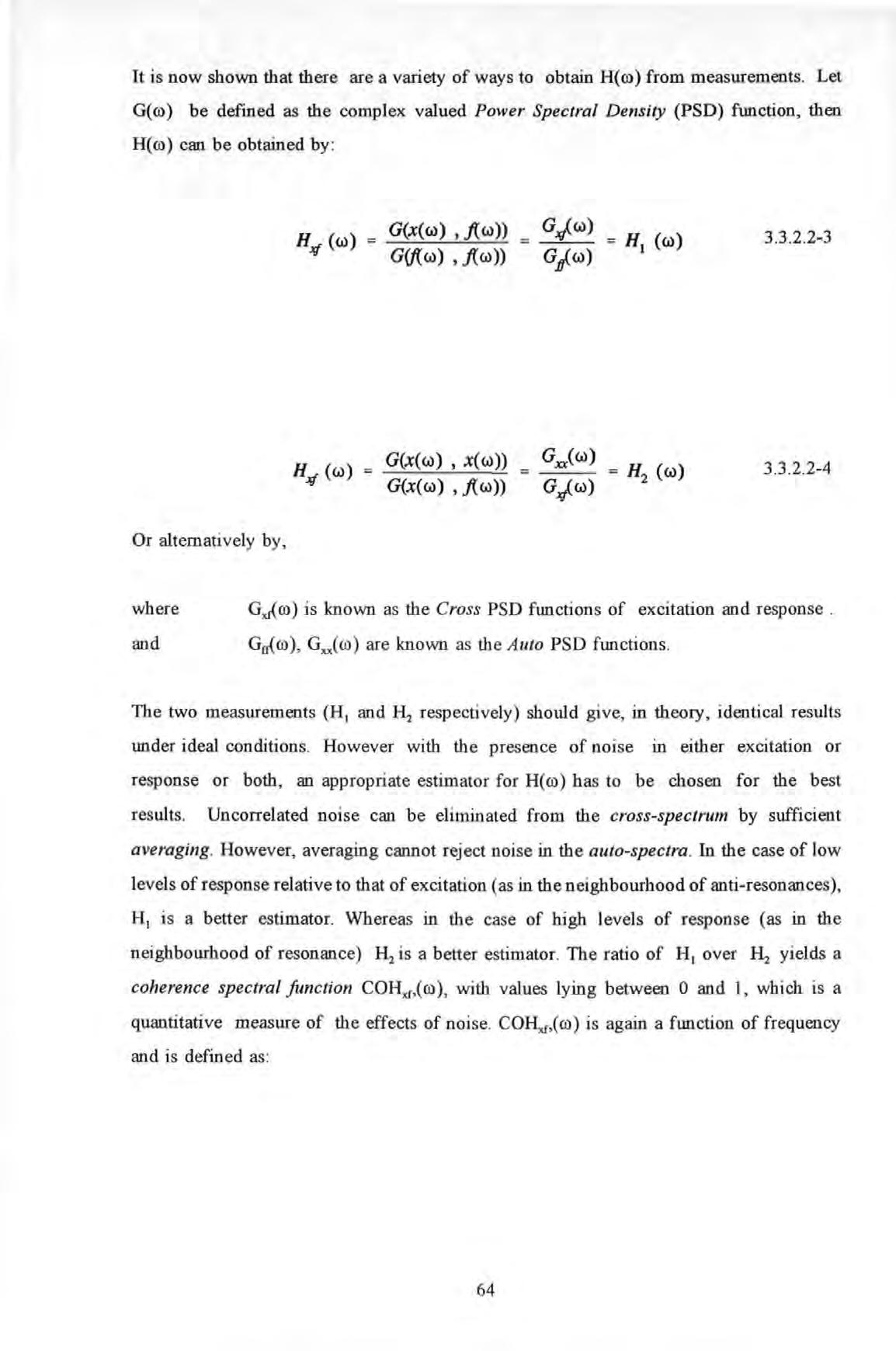
Or alternatively by , where and G,u{co) is known as the Cross PSD functions of excitation and response Ga( co ) , Gx.xC co) are known as the A uto PSD functions .

The two measurements (H 1 and respectively) should give, in theory , identical results under ideal conditions However with the presence of noise in either excitation or response or both , an appropriate estimator for H(co) has to be chosen for the best results. Uncorrelated noise can be eliminated from the cross-spectrum by sufficient averaging. However, averaging cannot reject noise in the auto-spectra . In the case of low levels of response relative to that of excitation (as in the neighbourhood of anti-resonances ), H 1 is a better estimator. Whereas in the case of high levels of response (as in the neighbourhood of resonance) a better estimator. The ratio of H 1 over yields a coherence spectral function co ), with values lying between 0 and 1, which is a quantitative measure of th e effects of noise COII,u,(co) is again a function of frequency and i s defined as :

A coherence value of I at a particular frequency means that the response and force have a very strong causality relationship and free from contamination of noise at that frequency . Whereas to the other extreme, a zero coherence means that there is no causality relationship between them . Low coherence is not only an indication of noise contamination but also non-linearity

For structural systems , the responses can be displacement x, velocity v, acceleration a, or other suitable quantities; whilst excitation is usually force f. By definition : ro) (or more commonly denoted as a ;j ) is called receptance, I:I_,t<ro) is called mobility , and HJ ro) is called accelerance or inertance

Once the measurement of these FRF at an array of spatial points of a structure is complete, parameter extraction can be proceeded in the way s as described in Chapter 5 and 6.

3.3.2.3 DATA ANALYSIS

The data analysis methods can broadly be classified into modal (or EMA) and non-modal (or Spatial) methods as defined in Section 1.2 EMA methods are well established techniques but non-modal methods are still to be developed further.

3.3.2.3.1 MODAL METHODS

EMA characterizes the dynamics of a structure in terms of its modal parameter set (i e undamped natural frequencies , modal damping factors and modal constants for each of the mode of vibration) In contrast to theoretical modal analysis, EMA determines these parameter set by experimental means and from experimentally measured Frequency

Response Functions

Historically, EMA techniques have undergone a gradual evolutionary process : from the early Sine Testing , Resonance Testing (see Raney '3 ' 12 ', Bishop and Gladwell 13 ' 131 ), Mobility testing (see Ewins '3' 141 ), Normal Mode Testing to Experimental Modal Analysis as it is called today.

The growing popularity of EMA is illustrated by the increase m the number of organised activities dedicated to this technology : notably the International Modal Analysis Conference (J tsJ which has been held annually since 1982 and the International Seminar On Modal Analysis 13 161 which has been held biannually since 1975 During the last decade, this technique has been widely applied to tackle a whole spectrum of engineering problems for modelling, troubleshooting and structural modification applications. Two new journals are published regularly on these subjects : The International Journal of Analytical and Experimental Modal Analysis 13' 171 and Mechanical Systems And Signal Processing . 13.1 11 These publications show that the proliferation of this technology to other disciplines and applications is ever increasing particularly when there is a need to validate results from theoretical modelling techniques . The founding theory of this approach will be dealt with later in chapter 5.

3.3.2.3.2 NON-MODAL METHODS

Non-modal (or spatial) method refer to one which does not use the idea of modes of vibration explicitly Usually , the identification process involves neither modal parameters determination nor the utilization of orthogonality properties of modes. The postulated mathematical model to fit is formulated in spatial rather than modal domain and is in terms of mass, stiffness and damping matrices of a structure. As for EMA , spatial method determine these parameter set from experimentally measured Frequency Response Functions also So the two Cl})proaches use the same data set. Spatial approach can be classified as direct parameter identification method. The founding theory of this approach will be dealt with later in chapter 6

It can be seen from the theoretical development in Section 3 .2.2 .2.2 that one can obtain the set of modal parameter (a modal model) by solving an eigenvalue problem posed in terms of the spatial matrices [M], [C] and [K] (a spatial model) A spatial model can also be obtained from a modal model if certain criteria can be met. The details on how this can be done will be further reviewed in Section 6. 1.3 .

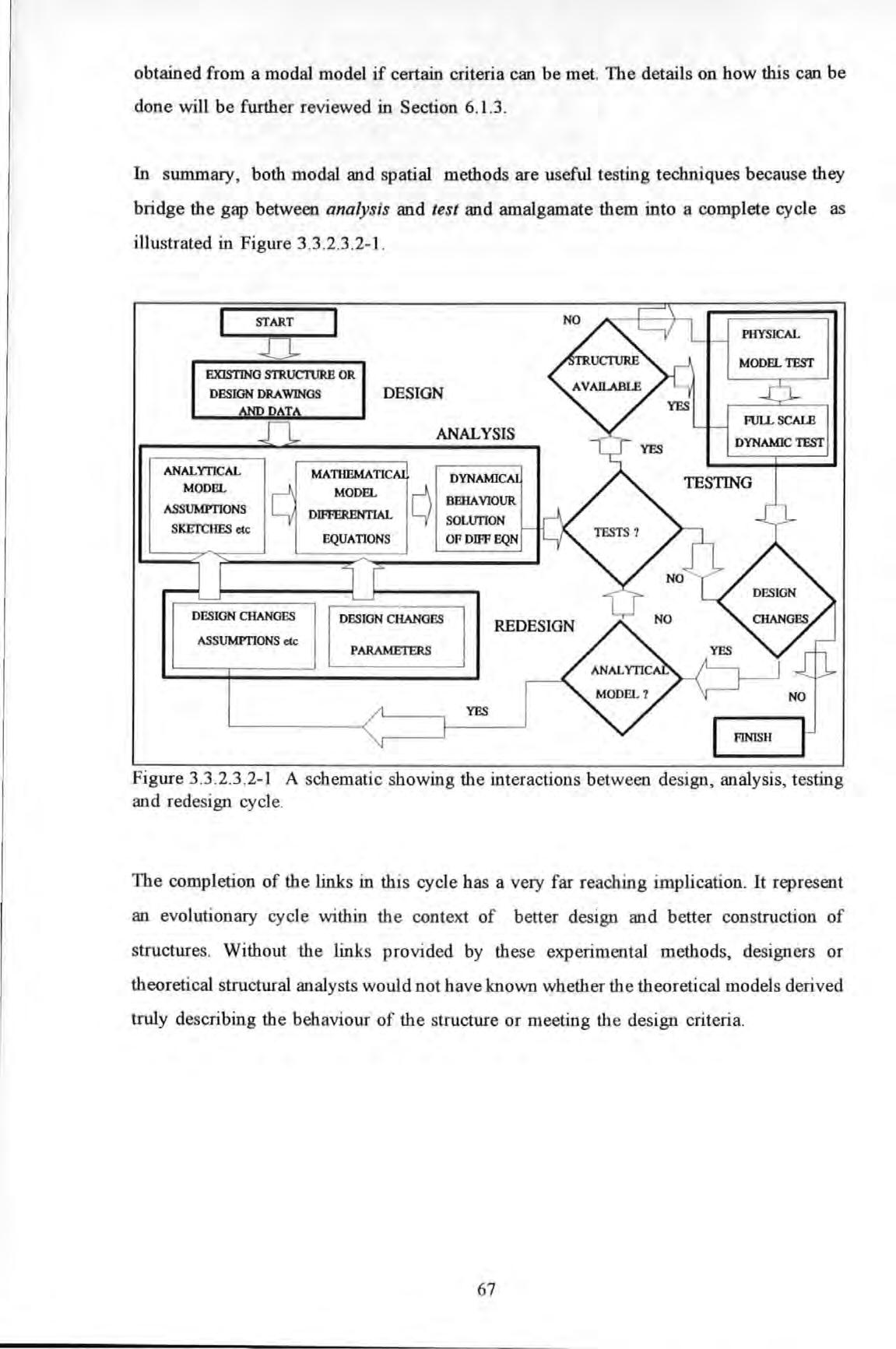
In summary , both modal and spatial methods are useful testing techniques because they bridge the gap between analysis and test and amalgamate them into a complete cycle as illustrated in Figure 3 3 2 3 2-1.

DESIGN CHANGES ASSUMPI'IONS etc

The completion of the links in this cycle has a very far reaching implication. It represent an evolutionary cycle within the context of better design and better construction of structures Without the links provided by these experim ental methods, design ers or theoretical structural analysts would not have known whether the theoretical models deriv e d truly describing the behaviour of the structure or meeting th e design criteria

Both theoretical and experimental methods can only be accurate if all the underlying assumptions are satisfied. Whilst this requirement can be met for simple structures, most engineering structures do not permit an accurate theoretical analysis.

Theoretical methods often produce spatial structural models of very large sizes. Damping assumed in these models is often not analytically derived but based on subjective assumptions. Theoretical modal models are obtained from theoretical spatial models via eigenvalue solutions and they too are of very large sizes. The technique of condensation of these large size matrices to smaller ones before carrying out a solution further introduce inaccuracies in these models.

Structural models obtained by the experimental methods introduced here, can either be in modal or spatial forms. The sizes of these models depend on the number of modes identified or number of coordinates measured and they are of much smaller sizes when compared with theoretical models. Both experimental modal and non-modal methods use the same experimental data set i.e. a set of frequency response functions measured at various coordinates of a structure. Therefore the same experimentation can be used for implementing the two techniques.

The basis of modal analysis is a linear transformation from an arbitrary coordinate space to normal coordinate space using the modal matrix and the utilisation of the orthogonality properties of the system's modes of vibration. In natural or normal coordinate space, modes are decoupled and this technique is called modal decoupling/decomposition. For undamped or proportionally damped systems, modal matrices are real. For generally damped or unproportionally damped systems, modal matrices are complex. Furthermore, orthogonality requires the system matrices to be symmetric which are generally true for most practical systems (with nonlinear systems as exceptions).

The validity of the experimental methods depends on the correct assumptions of a linear, second order and time-invariant system. Whilst few practical structures can perfectly fit all these assumptions, they should be borne in mind when applying these methods, especially when large discrepancies occur between the structures and their corresponding models.

Lastly, the experimental methods advocated here can be very useful supplements to though they may not be complete substitutes for theoretical methods.