Y5 Coastal Con: Technical Design Thesis- Abdullah Al Kazaz

Coastal Con ETS5 Thesis

Abdullah Al Kazaz

Architectural Association AA

Academic year 2023-24

Diploma Unit 4

Climate Peace

John Palmesino and Ann-Sofi Rönnskog

006 Introduction

Aim and Scope of Thesis

012 Chapter 1: Land Reclamation

1.1 Overview

1.2 Entities Behind Such Projects (Part 1)

1.3 Funding

1.4 Materials & Construction

1.5 Sea Level Rise

026 Chapter 2: Dubai: The Trigger Point

2.1 Introduction

2.2 Early Foundations and Regional Significance (Before 1900)

2.3 Economic Shifts and the Path to Modernization (1900-1950)

2.4 The Oil Discovery (1950-1970)

2.5 Strategic Development and Economic Boom (1971-1985)

2.6 Urban Expansion (1985-2000)

040 Chapter 3: The Palm Jumeirah Case Study

3.1 Introduction

3.2 Late 1990s- Historical Background & Planning

3.3 Early 2000s- Construction Phase

3.4 Mid 2000s to 2010- Completion & Initial Inhabitation

3.5 2010 Onwards

3.6 The Ignition Point

066 Chapter 4: Sample

4.1 Introduction

4.2 Multi-Temporal Composite

4.3 Land Classification Composite

4.4 The Overlay Process

094 Chapter 5: Global Coastal Surveillance

5.1 Introduction

5.2 Global Surface Water Project by the European Commission

5.3 Water Occurrence Change Intensity (1984-1999 to 2000-2021)

5.4 The Process

5.5 Analysis

124 Chapter 6: Global Coastal Extension Quantification

6.1 Introduction

6.2 Quantification

6.3 Results

6.4 Converting Pixels to Square Kilometers

6.5 Analysis

162 Chapter 7: Preventing Land Reclamation

7.1 Entities Behind Such Projects (Part 2)

7.2 Public-Private Partnership

7.3 Large-Scale Reclamation Projects: Problems Faced

7.4 Dominance of Luxury Housing

7.5 Garuda Jakarta

7.6 Urban Growth Boundary (UGB) Modification

180 Chapter 8: Conclusion

184 Bibliography

Aim

and Scope of Thesis

The aim of this thesis is to delve deeply into the processes of land reclamation driven by coastal real estate developments, examining their extensive implications on both natural environments and human settlements. A key focus is on quantifying and understanding the magnitude of material flux that results from such developments—how much earth is moved, the types of materials used, and where these materials are sourced. This analysis is crucial for assessing the ecological footprint and environmental impacts that accompany the expansion of coastal urban areas.

Additionally, this study aims to propose strategic intervention, including modifications to the Urban Growth Boundary (UGB), to gradually put an end to land reclamation.

The UGB is employed as a regulatory framework to control urban sprawl, preserve natural landscapes, and ensure sustainable growth by delineating areas that can be developed. Through this approach, the thesis will explore how altering the UGB in response to empirical data on land reclamation and material flux can lead to more balanced development practices that prioritize ecological sustainability alongside urban expansion.

Chapter 1: Land Reclamation

1.1 Overview

Land reclamation, a practice as ancient as it is modern, involves the conversion of aquatic spaces— oceans, riverbeds, or lake beds—into new land surfaces. Its primary motivation is to augment the available land to meet various needs, including agriculture, urban development, industrial zones, and infrastructure projects such as airports and ports. This expansion is particularly critical in regions where the demand for land, spurred by economic development and urban growth, outstrips the natural supply of usable terrain.

The process of land reclamation employs several techniques, each tailored to the specific characteristics of the area being developed and the intended use of the reclaimed land. These methods include the filling of water bodies with large quantities of earth and sand to raise the ground above water levels, the construction of seawalls and dykes to protect the new land from flooding, and the drainage of marshy or submerged areas.

Historically, land reclamation has been pivotal in the transformation and expansion of civilizations. In the Netherlands, a country where approximately 17% of its territory is land reclaimed from the sea or from lakes, this process has been instrumental in shaping national geography and living spaces. The Dutch have utilized a system of dykes, pumps, and windmills for

centuries to create arable land and habitable areas out of marshes and sea waters. The Zuiderzee Works and the Delta Works are among the most significant and sophisticated engineering projects in the world, showcasing advanced techniques in hydraulic engineering to protect reclaimed land from the sea.

Hong Kong presents another compelling example of land reclamation, driven by the scarcity of flat land and the pressures of urban expansion. Over 6% of Hong Kong’s total land area, including parts of its central business district and the region housing the Hong Kong International Airport, is built on reclaimed land. This has allowed the region to sustain its growth and maintain its status as a global financial hub despite geographical constraints.

Dubai’s ambitious land reclamation projects, such as the Palm Islands and The World archipelago, highlight a different aspect of land reclamation—luxury development and tourism. These projects have not only significantly increased Dubai’s coastline but also created unique residential, leisure, and entertainment spaces, contributing to its profile as a luxury tourist destination.

Despite the varied purposes and outcomes of land reclamation across different regions, the underlying motive remains consistent: to meet the ever-growing demand for land. Whether it’s for agricultural expansion, urban development, industrial use, or infrastructural projects, reclamation practices are a testament to human ingenuity in adapting their environments to meet their needs.

Fig. 1. An aerial view of construction and land reclamation by China in the South China Sea, as the country articulates its reasons for the expansions. ©ASIA MARITIME TRANSPARENCY INITIATIVE

3.

work in progress at a site in Hong Kong, highlighting concerns over the sustainability of material supplies. ©Ground Engineering

Fig.

Land reclamation

Fig. 2. Preparation for Addu City’s extensive land reclamation project is underway. ©Maldives Business Time

1.2 Entities Behind Such Projects (Part 1)

Land reclamation, the process of creating new land from oceans, riverbeds, or lakes, presents a complex, multifaceted operation involving a wide array of stakeholders. These entities range from government bodies at various levels to private sector participants and, in contemporary contexts, often include international consortia. Each plays a unique role, driven by a blend of policy objectives, economic considerations, and technical expertise.

National governments typically spearhead largescale land reclamation projects, leveraging significant resources and strategic planning capabilities. Their involvement usually aligns with broader national development objectives, such as enhancing infrastructure, expanding urban areas, or boosting economic zones. For instance, the government of Singapore, through agencies like the Urban Redevelopment Authority, has been instrumental in the country’s extensive land reclamation efforts aimed at accommodating its growing population and economic activities.

At the regional and local levels, authorities often initiate projects to address specific local needs, such as community development, recreational spaces, or local economic development. These projects might be smaller in scale but are crucial for the immediate societal and economic benefits they provide. The role of local government units in the Netherlands, working on

projects like the IJburg residential area in Amsterdam, illustrates local entities’ involvement in land reclamation for housing and urban development.

Private development companies, particularly those specializing in urban and coastal development, play a pivotal role in envisioning, financing, and executing reclamation projects. Their projects often aim at real estate development, commercial spaces, and leisure facilities. These entities rely on private investment and are motivated by the profit potential of developing reclaimed land. Emaar Properties in Dubai, known for projects like the Palm Jumeirah, exemplifies private sector involvement in ambitious reclamation efforts.

Engineering and construction firms bring the technical expertise required for the successful execution of land reclamation projects. These firms specialize in marine, environmental, and civil engineering, dealing with the complex challenges of building on reclaimed land, such as soil stabilization and flood protection. Companies like Boskalis Westminster and Van Oord have established reputations for their marine engineering and dredging capabilities on a global scale.

Increasingly, land reclamation projects are characterized by international partnerships that pool expertise, resources, and funding from around the globe. These consortia can include a mix of government entities, development companies, and engineering firms from different countries, working collaboratively towards common objectives. The Bandar Malaysia project in Kuala Lumpur, Malaysia, is an example where Chinese investment and international engineering expertise

have come together to develop a significant urban area.

The methodologies employed in land reclamation are as varied as the entities involved. Techniques range from the simple infilling of areas with sand or other materials to more complex methods involving the construction of seawalls and the subsequent pumping of sand behind these barriers. Collaboration among the diverse participants is crucial, as it allows for the integration of different skills, technologies, and resources. This collaborative approach is often coordinated through formal agreements, joint ventures, or public-private partnerships, ensuring that each entity’s strengths are effectively utilized to achieve the project’s goals.

Projects are typically underpinned by comprehensive planning processes, environmental impact assessments, and engineering studies, ensuring that the envisioned development is viable, sustainable, and capable of withstanding future challenges. This preparatory work is critical for aligning the diverse objectives and expectations of the various stakeholders involved in a project.

1.3 Funding

Land reclamation, the process of creating new land from oceans, seas, riverbeds, or lake beds, involves a complex and multifaceted funding landscape. The financial backbone of these projects comprises a diverse mix of public and private funding sources, reflecting the varied nature and objectives of reclamation efforts.

Public funding for land reclamation projects is typically allocated by government entities at various levels, including local, regional, and national governments. This funding is earmarked for projects deemed to have significant public benefits. For example, flood protection initiatives aim to safeguard communities from the devastating impacts of natural disasters, thereby mitigating potential economic losses and ensuring public safety. Similarly, the creation of public infrastructure, such as roads, bridges, and parks, serves to enhance community accessibility, connectivity, and overall quality of life.

Governments may allocate funds for these projects through direct budgetary provisions or through specific funding programs designed to support infrastructure development and environmental conservation efforts. For instance, the European Union has mechanisms like the Cohesion Fund and the European Regional Development Fund, which support large-scale infrastructure projects, including those involving land

reclamation, in member states with a focus on sustainable development and cohesion among regions. On the other hand, private land reclamation projects, often aimed at residential or commercial development, rely heavily on funding from the developers undertaking these projects. These developers may invest their own capital or seek external financing to cover the costs associated with land reclamation. External financing can come from a variety of sources, including banks, private equity firms, and other financial institutions, which provide loans or invest in projects in anticipation of future returns generated by the developed property.

In addition to direct project costs, developers must also account for the expenses related to environmental assessments and planning. These assessments are crucial for identifying potential environmental impacts of the reclamation project and for developing strategies to mitigate these impacts. The planning phase involves detailed analysis and design work to ensure the feasibility and sustainability of the project, encompassing aspects such as land use planning, infrastructure design, and environmental protection measures.

The overall investment in land reclamation projects encompasses a broad range of costs. The physical construction costs include the expenses associated with earthmoving, dredging, soil stabilization, and the construction of necessary infrastructure such as seawalls and drainage systems. Environmental assessment costs cover studies to evaluate the project’s impact on local ecosystems, water quality, and biodiversity. These assessments are essential for obtaining

the necessary environmental permits and for ensuring compliance with environmental regulations.

Planning costs entail the expenses related to the development of detailed project plans, including feasibility studies, design work, and stakeholder consultations. Additionally, projects may incur costs associated with mitigation measures designed to address environmental impacts. These measures can include habitat creation or restoration, pollution control efforts, and the implementation of sustainable development practices to minimize the project’s ecological footprint.

Funding mechanisms for land reclamation projects vary widely, depending on the project scale, objectives, and geographical location. For public projects, funding may come from tax revenues, government bonds, or international grants. Private projects often leverage project financing structures, where the project’s assets, rights, and interests are used as collateral to secure financing.

1.4 Materials & Construction

The sourcing of materials for land reclamation represents a pivotal phase within the broader scope of project planning and execution. This process involves a meticulous evaluation of available resources, environmental considerations, and the specific engineering demands of the project. The sequence of operations extends from initial concept development through to project execution and ultimately, the handover of the reclaimed land.

The initial phase entails a comprehensive feasibility study where the project’s objectives are defined. This stage considers the proposed area for reclamation and the intended use of the newly created land, whether for residential, commercial, industrial, or recreational purposes. During this period, preliminary assessments of potential material sources are conducted to ensure the project’s viability.

Riverbeds and Coastal Areas: Local sourcing involves extracting materials such as sand, gravel, and rocks from nearby riverbeds and coastal areas. This method is favored due to lower transportation costs and reduced carbon footprint. The selection of local materials is subject to rigorous testing to ensure they meet the structural and durability requirements of the reclamation project.

Construction and Demolition Waste: Another local

sourcing option includes the use of recycled materials from construction and demolition waste. This method not only contributes to the sustainability of the project but also helps in managing waste effectively.

In instances where local materials do not meet the technical or environmental standards required for the project, materials are imported from other regions or countries. Imported materials are usually selected based on their specific properties, such as grain size and composition, which are critical for ensuring the stability and longevity of the reclaimed land. The process of importing materials involves logistic considerations, including transportation routes, shipping methods, and the environmental impact of long-distance transport.

An Environmental Impact Assessment (EIA) is integral to the material sourcing process. The EIA evaluates the potential environmental repercussions of extracting materials, both locally and imported. It encompasses an analysis of biodiversity impacts, water quality, sediment displacement, and the carbon footprint associated with transportation. The findings from the EIA can influence the selection of materials, pushing the project towards more sustainable practices.

The technical specifications of the project dictate the choice of materials. These specifications are determined by the engineering requirements of the land reclamation, such as load-bearing capacity, erosion resistance, and compatibility with the existing environment. Quality control measures are implemented to ensure that all sourced materials adhere to the

Fig. 4. Extraction and transportation of construction materials for potential use in land reclamation projects, highlighting the sourcing of raw materials necessary for such developments. ©maltatoday

project’s technical standards. This includes laboratory testing of material properties, on-site inspections, and continuous monitoring throughout the project’s lifecycle.

Following the sourcing and testing of materials, the project execution phase commences. This phase involves the physical act of land reclamation, utilizing the sourced materials to create new land masses. Techniques such as hydraulic filling, where materials are mixed with water and pumped to the reclamation site, are commonly employed. Throughout this phase, project management teams oversee the operation, ensuring adherence to the planned timeline, budget, and quality standards.

Upon completion of the reclamation project, a thorough review is conducted to ensure that the newly reclaimed land meets all the technical and environmental criteria set forth in the planning stages. This includes final quality assurance tests and an evaluation of the environmental impact post-construction. The handover process concludes with the transfer of the reclaimed land to the client or governing body, accompanied by all necessary documentation and certifications.

Fig. 5. Marine land reclamation process utilizing geotextiles and dredging methods to create new land areas. ©SIDCO

Fig. 6. Dredging vessel at work, actively depositing sediment to form new land along a coastal area. ©IADC

Fig. 7. Excavators managing the distribution of sand pumped ashore for a coastal land reclamation project, with a dredging ship in the background. ©Ground Engineering

1.5 Sea Level Rise

Land Reclamation carries with it a set of ecological repercussions that can exacerbate the problem of rising sea levels—a critical issue in the context of global climate change.

Impact on Coastal Ecosystems

Coastal ecosystems like mangroves, tidal marshes, and wetlands are not merely features of a landscape; they play a pivotal role in stabilizing shorelines, buffering against storm surges, and regulating water levels. These ecosystems are dynamic interfaces where land and water meet, teeming with life and biodiversity. They are capable of sequestering significant amounts of carbon, thus also contributing to the mitigation of climate change.

When land reclamation projects are initiated, they often result in the destruction of these vital ecosystems. The infill material used for land reclamation smothers benthic habitats, displaces fauna, and halts the natural processes of sediment deposition and erosion. Moreover, the loss of vegetation due to reclamation leads to the reduction of natural carbon sinks, potentially increasing greenhouse gas concentrations in the atmosphere.

Without the protection and absorption capabilities of these coastal buffers, areas become more vulnerable

to the impacts of storm surges. As a result, the natural defense against the encroachment of sea waters is weakened, leading to accelerated coastal erosion. The eroded materials contribute to sedimentation elsewhere, potentially affecting ocean currents and further disturbing the coastal balance. These processes can lead to local, and possibly regional, rises in sea levels.

Volume Displacement and Sea Level Rise

The principle of displacement suggests that when an area is filled for land reclamation, the volume of water that was once occupying that space is pushed elsewhere. This is akin to pressing down on one end of a water-filled balloon—the water doesn’t disappear; it simply moves to another part of the balloon. On a global scale, the displacement isn’t so straightforward because of the sheer volume of the oceans, but the principle remains the same.

Land reclamation can result in a physical increase in the water volume within the ocean basins. While each individual reclamation project may only displace a small amount of water relative to the volume of the world’s oceans, the cumulative effect of many such projects around the world can contribute to measurable changes in sea levels.

Additionally, the increase in impervious surfaces due to urbanization leads to less water being absorbed into groundwater reserves, resulting in more runoff directly into the ocean. This, combined with the thermal expansion of water due to increased global temperatures, can contribute to an overall rise in sea levels.

Fig. 8. Map by the European Space Agency showing sea level trends from September 1992 to January 2018. Regions in red and orange indicate rising sea levels, while areas in blue show sea levels falling. The map uses a scale from -10 to +10 millimeters per year to indicate the magnitude of change. ©ESA

Secondary Impacts and Long-term Implications

Secondary impacts of land reclamation include changes to local hydrology and alterations in groundwater systems. By changing the landscape, reclamation projects can alter the flow of rivers and streams, potentially leading to increased sedimentation in some areas and erosion in others. These alterations can change the salinity of coastal waters, impacting marine life and potentially leading to a decline in fisheries—a vital food source for millions of people.

The long-term implications of continued land reclamation are profound. As sea levels rise, the reclaimed land, often not much above sea level, becomes increasingly at risk of flooding and subsequent damage. This creates a cycle where more defenses are needed, leading to further environmental degradation, loss of biodiversity, and increased vulnerability to sea level rise.

Given these multifaceted impacts, the practice of land reclamation requires a reevaluation of its long-term viability and sustainability. Policymakers and developers must balance economic development with the need to protect and restore natural ecosystems. Adopting green reclamation techniques, such as creating wetland reserves or using eco-friendly materials, could mitigate some of the negative impacts, but the focus should be on preserving natural coastlines where possible.

Effective management strategies and international cooperation are essential to address the complex chal-

lenges posed by land reclamation and sea level rise. By prioritizing ecological integrity alongside human development, we can work towards a more sustainable coexistence with the natural world.

Fig. 9. Graph depicting projected global mean sea level rise under different SSP (Shared Socioeconomic Pathways) scenarios, from the IPCC (Intergovernmental Panel on Climate Change) report “Climate Change 2021: The Physical Science Basis.” ©IPCC

1.6 Global Total Reclaimed Land Map

9. Recreation from a research paper. The map is marked with orange circles of varying sizes, each representing a different amount of land that has been reclaimed. The key at the bottom left suggests that the size of the circles corresponds to the scale of land reclamation: large circles for areas greater than 100 square kilometers, medium circles for areas between 5 to 100 square kilometers, and small circles for less than 5 square kilometers. The map highlights significant reclaimed land areas particularly concentrated along coastlines and estuaries, indicating human activity in modifying landscapes for various purposes such as agriculture, urban development, or other uses. ©AUGPublications

Fig.

Chapter 2: Dubai:

The Trigger Point

2.1 Introduction

Nestled at the crossroads of East and West, Dubai’s strategic geographical location on the southeastern coast of the Persian Gulf has historically positioned it as a vital trading hub. Its coastal lineage, characterized by a long, winding creek extending into the heart of the desert, has not only shaped its topography but also its destiny. From its early days as a modest fishing village, Dubai’s natural harbor facilitated regional trade routes, laying the foundation for a society deeply rooted in trade and commerce. This early inclination towards trade was further bolstered by the rich pearling beds along its coast, drawing merchants from across the region and beyond.

As the 20th century unfolded, Dubai’s narrative took a dramatic turn. The discovery of oil in the late 1960s catalyzed a series of infrastructural and economic transformations, propelling the emirate onto the global stage. However, unlike many of its neighbors, Dubai’s foresight in economic diversification has been pivotal. Even before oil reserves would define the region’s wealth, Dubai’s leadership envisioned a future less dependent on this finite resource. Investments in ports, free zones, and eventually, a slew of audacious development projects, marked the beginning of a new era.

By the turn of the 21st century, Dubai had already laid the groundwork for its metamorphosis into a bustling metropolis, renowned for its skyscrapers, luxury, and a seemingly insatiable appetite for groundbreaking

projects. The city’s historical reliance on trade and strategic geographic advantages had evolved, setting the stage for ambitious urban and coastal development projects. These endeavors not only aimed to redefine the city’s skyline but also to solidify its position as a pivotal global nexus for finance, tourism, and culture. As Dubai stood on the brink of a new millennium, it was poised for a period of unprecedented growth that would challenge conventional notions of urban development and land reclamation, marking the beginning of its most transformative chapter yet.

2.2 Early Foundations & Regional Significance (Before 1900)

1833-1892: The Bani Yas Settlement and Early Development

In the early 19th century, the vast and arid landscapes of what is now known as Dubai were primarily inhabited by nomadic Bedouin tribes, traversing the desert in search of water and seasonal vegetation. This all changed in 1833 when approximately 800 members of the Bani Yas tribe, led by the Maktoum family, settled by the banks of the Dubai Creek. This strategic move was motivated by the creek’s natural harbor, which offered protection from the Gulf’s rough seas and an ideal location for fishing and pearling. The Maktoum family’s leadership, under Sheikh Maktoum bin Butti, established a foundation of governance that would guide Dubai’s development for centuries to come.

This nascent settlement quickly transformed into a bustling fishing village, leveraging its geographical advantages to emerge as a pivotal point in regional trade routes. The abundant marine resources attracted merchants and traders from across the region, setting the stage for Dubai’s future as a center of commerce and trade.

The importance of Dubai in regional trade was further

cemented with the signing of the General Maritime Treaty with Britain in 1820, followed by a series of agreements that extended into the mid-19th century. These treaties were designed to combat piracy along the Gulf coast, ensuring safe passage for British vessels and, by extension, stabilizing the region. For Dubai, the treaties brought a measure of external protection that allowed its trade to flourish. The British influence also introduced a semblance of international maritime law, which contributed to the emirate’s growing reputation as a reliable trading hub.

Late 19th Century: The Pearling Boom

By the late 19th century, Dubai had established itself as a vital cog in the regional trade machine, with its economy experiencing a significant boost from the pearling industry. The warm waters of the Persian Gulf were home to some of the world’s richest pearl beds, and Dubai’s strategic location made it a central marketplace for the pearling trade. Pearls from Dubai were highly sought after, not only in the Gulf region but also in Europe and Asia, further expanding Dubai’s trade networks.

The pearling industry also marked Dubai’s first foray into a structured economy. During the pearling season, which ran from June to September, the city’s population would swell as divers, boat builders, and traders converged on Dubai. The wealth generated from pearling contributed to the development of infrastructure and the establishment of Dubai as a regional trading center. Moreover, the pearling industry fostered a diverse, multicultural community as it attracted

Fig. 10. Dubai Creek, 1960. ©Pinterest

workers and traders from various ethnic and social backgrounds.

However, the prosperity brought by pearling was not without its challenges. The industry was labor-intensive and perilous, with divers facing significant risks for minimal rewards. Additionally, the success of the pearling industry made Dubai’s economy vulnerable to fluctuations in global markets.

As the 19th century drew to a close, Dubai was poised on the brink of modernization. The foundation laid by the Bani Yas tribe, combined with the wealth and international connections fostered by the pearling industry, had transformed the once-sleepy fishing village into a burgeoning trade center. This period of early foundations and regional significance set the stage for Dubai’s remarkable transformation in the 20th century, as it navigated the challenges of economic diversification and embraced the opportunities of global integration.

Fig. 11. Ships in 1967 unloading goods on the creek for the Customs Department in Dubai. ©The National News

2.3 Economic Shifts and the Path to Modernization (19001950)

1900s-1930s: The Dawn of Modernization under Sheikh Maktoum bin Hasher Al Maktoum

The turn of the 20th century marked a pivotal era in Dubai’s history, characterized by visionary leadership and strategic initiatives that laid the groundwork for its future as a global city. Under the rule of Sheikh Maktoum bin Hasher Al Maktoum, who assumed power in 1894, Dubai embarked on a series of modernization efforts that would redefine its economic and social landscape.

One of Sheikh Maktoum’s most transformative projects was the development of Dubai Creek, a natural inlet that had long been the lifeblood of the city’s economy. Recognizing the creek’s potential to bolster trade, Sheikh Maktoum initiated a bold dredging project in the early 20th century to deepen the channel, allowing larger vessels to navigate its waters. This not only enhanced Dubai’s accessibility to international shipping but also established the emirate as a crucial maritime trade hub in the Gulf region.

The expansion of Dubai Creek was accompanied by infrastructural developments that facilitated trade and commerce. The establishment of the first custom

house and the introduction of formal trade licenses created a more organized and attractive environment for merchants from around the world. This era also saw the construction of new souks and trading posts along the creek’s banks, further stimulating economic activity.

Sheikh Maktoum’s modernization efforts extended beyond infrastructure to include the adoption of progressive policies that attracted foreign traders and settlers. By granting tax exemptions and offering land grants, he encouraged a wave of immigration that brought skilled laborers, entrepreneurs, and families to Dubai, contributing to a melting pot of cultures and expertise.

1930-1950: Economic Turbulence and the Quest for Diversification

The global economic landscape of the early 20th century, however, posed significant challenges to Dubai’s burgeoning economy. The Great Depression of the 1930s sent shockwaves through the world’s markets, severely impacting Dubai’s pearling industry. The advent of cultured pearls in the 1920s by Japanese innovators further exacerbated the situation, leading to a precipitous decline in demand for natural pearls. The once-thriving pearling industry, which had been a cornerstone of Dubai’s economy, was suddenly faced with obsolescence, leaving thousands of divers and traders without livelihoods.

The decline of the pearling industry served as a stark wake-up call for Dubai’s leadership, highlighting the dangers of economic dependence on a single com-

Fig. 12. Protective walls were built on Dubai Creek in 1960, such as this one, to protect against sea erosion. This was taken on the Bur Dubai side. ©The National News

Fig. 13. This historical map outlines proposed improvements for Dubai Harbour, including the construction of groynes and dredging areas, with details of existing structures and areas prone to tidal flooding. It provides a detailed layout for the development of the harbour and adjacent lagoon. ©Getty Images

modity. It set the stage for a pivotal shift in the emirate’s economic strategy, with a renewed focus on diversification and sustainable development.

The 1940s marked the beginning of Dubai’s foray into oil exploration, a venture that would eventually redefine its economic landscape. Initial exploratory activities were met with skepticism, given the technical and financial challenges involved. However, the persistence of Dubai’s rulers in pursuing oil exploration was driven by a vision of economic transformation and stability. While the discovery of oil in commercial quantities would not occur until the 1960s, the initial steps taken in this period laid the foundation for Dubai’s future as an oil-producing state.

2.4 The Oil Discovery (19501970)

1958-1966: The Era of Black Gold

The late 1950s and early 1960s heralded a new chapter in Dubai’s storied history, one that would forever alter its socioeconomic landscape. The discovery of oil in the region, particularly the significant find in 1966 at the offshore field named Fateh, marked the dawn of a transformative era. This discovery came after years of exploration, fueled by the persistent belief in Dubai’s potential to join the ranks of oil-producing states. The first oil exports in 1969 represented a pivotal moment, symbolizing Dubai’s entry into the global oil economy.

The influx of oil revenue had an immediate and profound impact on Dubai’s economy and infrastructure. For a city that had historically relied on trade, pearls, and fishing, the newfound wealth presented an unprecedented opportunity for development. Sheikh Rashid bin Saeed Al Maktoum, the then-ruler of Dubai, demonstrated visionary leadership by channeling oil revenues into comprehensive infrastructural development. The early focus was on creating a robust foundation for future growth, which included the construction of roads, schools, and hospitals.

The establishment of the first modern highway, linking Dubai with the neighboring emirate of Abu Dhabi,

revolutionized transportation and connectivity within the region. Education and healthcare received significant boosts, with the construction of modern facilities designed to meet international standards. These infrastructural developments not only improved the quality of life for Dubai’s residents but also made the emirate more attractive to foreign investors and expatriates.

Late 1960s: Visionary Leadership and Diversification

Even as oil began to flow and transform the economic landscape, Sheikh Rashid bin Saeed Al Maktoum was acutely aware of the pitfalls of over-reliance on a single resource. Drawing from Dubai’s rich history of trade and commerce, he embarked on an ambitious journey to diversify the economy and invest in sustainable development.

One of Sheikh Rashid’s most significant projects was the further expansion of Dubai Creek. Recognizing the limitations imposed by the natural creek on trade and shipping activities, he initiated a bold dredging project that would deepen and widen the creek, allowing larger vessels to dock. This expansion, completed in the late 1960s, revitalized Dubai’s port facilities and reinforced its status as a major trading hub in the region.

Sheikh Rashid’s vision extended beyond physical infrastructure. He implemented policies that encouraged foreign investment and fostered a businessfriendly environment. The establishment of the Jebel Ali Free Zone in the 1970s, although beyond the

Fig. 14. Oil was pumped from the barge into the Sand Bund. Sheikh Rashid’s people could now see their newly discovered crude flowing. ©DubaiAsItUseToBe

scope of this period, was conceptualized during this time as a testament to Dubai’s commitment to trade diversification and economic openness.

The period between 1958 and 1970 was, therefore, one of profound transformation for Dubai. The discovery of oil served as the catalyst for development, but it was the strategic vision of Sheikh Rashid bin Saeed Al Maktoum that laid the groundwork for Dubai’s rise as a diversified and dynamic global city. Through investments in infrastructure, education, and healthcare, coupled with a steadfast commitment to economic diversification, Dubai set itself on a path of sustainable growth that would continue to define its trajectory in the decades to come. This era underscored the importance of visionary leadership and strategic planning in harnessing natural wealth for the longterm prosperity of a nation.

Fig. 15. That Dubai had discovered oil reserves was now a reality. But that reality existed 15 miles offshore. ©DubaiAsItUseToBe

2.5 Strategic Development and Economic Boom (19711985)

The year 1971 stands as a watershed moment in Dubai’s history, marking the birth of the United Arab Emirates (UAE). On December 2, 1971, Dubai joined Abu Dhabi and five other emirates in forming a new federation, signaling a new era of unity and collective ambition. This historic union was catalyzed by the visionary leadership of Sheikh Zayed bin Sultan Al Nahyan of Abu Dhabi and Sheikh Rashid bin Saeed Al Maktoum of Dubai, among others. Dubai’s strategic geographical location and its burgeoning economy made it a pivotal member of the federation, offering significant maritime access and trade capabilities to the collective.

The formation of the UAE was more than a political milestone; it was a strategic alliance that pooled resources and ambitions, setting the stage for a transformative economic trajectory. For Dubai, this meant an opportunity to amplify its development efforts, leveraging the federation’s collective oil wealth while maintaining its unique focus on trade and infrastructure development.

1970s: A Decade of Infrastructure and Trade Ex-

pansion

The 1970s were characterized by an aggressive push towards infrastructural development, significantly bolstered by the federation’s oil revenues and Sheikh Rashid’s visionary leadership. Central to Dubai’s strategy was the enhancement of its maritime capabilities, recognizing the emirate’s historical reliance on trade and its ambition to become a global hub for commerce and logistics.

Jebel Ali Port: Inaugurated in 1979, Jebel Ali Port was a monumental project that reflected Dubai’s grand ambitions on the global stage. Designed to be the largest man-made harbor in the world, Jebel Ali Port was not just about scale; it was strategically positioned to serve the East-West trade routes, equipped with state-of-the-art facilities capable of accommodating the largest cargo ships of the time. This development catapulted Dubai into the league of major international ports, offering unprecedented access to global markets.

Dubai Drydocks: Complementing the maritime infrastructure, the Dubai Drydocks, established in 1978, was another strategic investment. As the most extensive ship repair facility in the Middle East, the Drydocks underscored Dubai’s comprehensive vision for maritime services, catering not only to logistics but also to maintenance and servicing, further enhancing its appeal as a global maritime center.

Jebel Ali Free Zone (JAFZA): Perhaps the most visionary of Sheikh Rashid’s initiatives was the estab-

Fig. 16. Jebal Ali Port, 1979 ©Gulf News

1971: The Formation of the United Arab Emirates

lishment of the Jebel Ali Free Zone in the early 1980s. JAFZA was designed as a fully integrated business hub, offering unparalleled incentives for international corporations, such as 100% foreign ownership, full repatriation of profits, and exemption from importexport duties. This bold move was instrumental in attracting foreign investment, transforming Dubai into a crucible of international business activity.

The period from 1971 to 1985 was marked by strategic development initiatives that leveraged Dubai’s historical strengths while positioning it for future growth.

The establishment of the UAE provided a platform for unity and collective progress, which Dubai capitalized on through ambitious infrastructural projects.

The completion of Jebel Ali Port, alongside the Dubai Drydocks and Jebel Ali Free Zone, marked a significant leap in Dubai’s economic development. These projects were not just about enhancing Dubai’s maritime capabilities; they were a clear signal of its global ambitions and its commitment to becoming a hub for international trade and investment. Through these visionary projects, Dubai laid the foundational stones of its future as a dynamic, diversified economy, setting the stage for unprecedented growth and development in the decades to follow.

Fig. 17. Jebal Ali Port, 1979 ©Gulf News

Fig. 18. The growth of Dubai’s economy from 1975 to around 2008. The lines show a relatively steady increase up to the year 2000, followed by a significant rise in all three indicators in the years after. The blue line represents Real GDP, the red line for Capital, and the green line for Employment, indicating all have seen substantial growth over the period, especially post-2000. ©ResearchGate

2.6 Urban Expansion (19852000)

1985-1990: Skyward Ambitions - Dubai International Airport and Emirates Airline

The mid-1980s marked the beginning of Dubai’s ambitious journey to become a nexus of global connectivity. Central to this vision was the expansion of Dubai International Airport and the launch of Emirates Airline, both of which played pivotal roles in opening Dubai to the world.

Dubai International Airport Expansion: Recognizing the strategic importance of aviation infrastructure in global commerce and tourism, Dubai embarked on a significant expansion of its international airport. The upgrade included the addition of new terminals, advanced aviation technology, and increased capacity, transforming it into one of the busiest and most advanced airports globally. This expansion was not merely about accommodating more passengers; it was a clear statement of Dubai’s ambition to serve as a global crossroads.

Launch of Emirates Airline (1985): The establishment of Emirates Airline was a bold venture into the competitive aviation industry, funded by the Dubai government with an initial investment and two borrowed aircraft. Under the visionary leadership of Sheikh Mohammed bin Rashid Al Maktoum, Emirates

quickly expanded its fleet and destinations, focusing on service quality and connectivity. The airline’s growth mirrored that of Dubai, as it connected the emirate to key cities worldwide, facilitating trade, tourism, and investment flows.

1990s: The Digital and Media Revolution - Dubai Internet City and Dubai Media City

The 1990s witnessed a strategic pivot towards technology and media, marking the beginning of Dubai’s transformation into a global city of the future. The launch of Dubai Internet City (DIC) and Dubai Media City (DMC) was instrumental in this transition, positioning Dubai as a hub for innovation and communication.

Dubai Internet City (1999): DIC was established as a free economic zone for technology companies, offering state-of-the-art infrastructure, business services, and a regulatory environment designed to foster innovation and entrepreneurship. By attracting leading global technology firms and startups, DIC catalyzed the growth of the information technology sector in the region.

Dubai Media City (2000): Similarly, DMC was created as a hub for media organizations, including news agencies, publishing, online media, broadcasting, and production companies. It provided a collaborative ecosystem that encouraged creativity and content creation, contributing to Dubai’s emergence as a regional and global media center.

Fig. 19. A time series from January 2003 to December 2010, plotting a metric that rises significantly from 2007, peaks in 2008, and then declines, though not to previous levels. ©ResearchGate

Late 1990s

As the 20th century drew to a close, Dubai’s leadership envisioned a series of urban development projects that would redefine the concept of city-building. Among these was the Palm Jumeirah, an ambitious land reclamation project that symbolized Dubai’s audacity and vision.

Conceived in the late 1990s, Palm Jumeirah was an engineering marvel and a testament to Dubai’s ambition to create the unprecedented. Planned as the world’s largest artificial island, it was designed to significantly increase Dubai’s shoreline and provide luxury residential, leisure, and tourism facilities. The project not only showcased Dubai’s capacity for groundbreaking development but also set a new benchmark for urban expansion and creativity.

The period from 1985 to 2000 was characterized by strategic foresight and bold initiatives that propelled Dubai onto the global stage. The expansion of Dubai International Airport and the launch of Emirates Airline enhanced the emirate’s global connectivity, paving the way for its emergence as an international aviation hub. The establishment of Dubai Internet City and Dubai Media City marked the beginning of Dubai’s transformation into a global city, embracing the digital age and the media revolution. Meanwhile, the conceptualization and planning of projects like Palm Jumeirah exemplified Dubai’s visionary approach to urban development, setting the stage for a new era of architectural and infrastructural marvels. This phase of urban expansion and strategic development laid

the foundational pillars for Dubai’s rapid growth in the 21st century, cementing its status as a dynamic, innovative, and globally connected city.

Chapter 3: The Palm Jumeirah Case

Study

3.1 Introduction

Conceived in the late 1990s under the visionary guidance of Sheikh Mohammed bin Rashid Al Maktoum, the USD 12 billion Palm Jumeirah was designed not only to expand Dubai’s coastline but also to redefine the emirate as a global hub for tourism and luxury living. Developed by Nakheel Properties, a governmentowned real estate titan, the project was emblematic of Dubai’s aspirations to etch its name on the world stage as a premier destination.

This chapter aims to dissect the development journey of the Palm Jumeirah, from its inception to its completion and beyond, with a focus on the 1990s through 2010. The analysis will delve into the project’s phases, challenges, achievements, and particularly its environmental impact. The Palm Jumeirah, while a marvel of engineering, has also been a point of contention, emblematic of the intricate dance between large-scale anthropogenic development and the delicate balance of coastal ecosystems.

The Palm Jumeirah’s inception was driven by Dubai’s strategic objective to diversify its economy and solidify its status as a leading tourist and luxury living destination. The project’s ambitious design, symbolizing a palm tree nestled within a crescent, was both a marvel of aesthetic appeal and engineering brilliance. Initiated with the dredging and reclamation of 1,380 acres from the sea, this endeavor was unparalleled in

its scope, demanding innovative solutions to substantial engineering and environmental challenges.

The construction of the Palm Jumeirah was a narrative of overcoming seemingly insurmountable obstacles. From managing ocean currents and ensuring land stability to addressing rising sea levels, the project navigated a myriad of technical and environmental challenges. The use of ground improvement techniques, such as vibrocompaction, and the innovative creation of a new 60-kilometer coastline, highlighted the project’s engineering complexity and its environmental foresight.

However, the engagement with the natural environment was not without its critiques. The massive reclamation efforts and alterations to the coastal landscape prompted concerns about the sustainability of such developments and their long-term impact on marine ecosystems and erosion patterns.

As the Palm Jumeirah evolved into a vibrant community, home to 8,000 villas, apartment complexes, and numerous commercial establishments, its environmental implications became increasingly apparent. The project, while enhancing Dubai’s appeal as a luxury destination, also raised critical questions about the interactions between human-made developments and natural ecosystems. The anticipated coastal erosion and the subsequent construction of the world’s largest artificial reef to mitigate this erosion underscored the ongoing struggle to balance development ambitions with environmental stewardship.

Fig. 20. Stylized promotional map showing Palm Jumeirah and nearby Dubai landmarks with travel times: “WHERE THE CITY MEETS THE SEA”. ©InvestDXB

The Palm Jumeirah represents a monumental achievement in engineering and real estate development. It embodies Dubai’s relentless pursuit of innovation and luxury, redefining the city’s skyline and identity. Yet, it also serves as a poignant reminder of the complex relationship between human ambition and the natural world. The project’s environmental challenges and interventions highlight the pressing need for sustainable development practices that harmonize with the ecological realities of our planet.

As we move forward, the Palm Jumeirah’s legacy offers valuable lessons in the realms of engineering, environmental science, and urban planning. It prompts a critical examination of how large-scale developments interact with and impact coastal ecosystems. This case study, emblematic of the problematic interactions between human developments and coastal ecosystems, underscores the imperative for ongoing research, innovation, and dialogue to navigate the fine balance between achieving human aspirations and preserving the natural environment.

Fig. 21. Aerial view of the early stages of Palm Jumeirah’s construction, showing land reclamation with breakwaters and sand shaping. ©Hostel-Bereg

3.2 Late 1990s- Historical Background & Planning

At the heart of this ambitious project was Nakheel Properties, a real estate juggernaut owned by the Government of Dubai, and the visionary American architectural firm Helman Hurley Charvat Peacock (HHCP). Together, they embarked on a journey to materialize a grand vision: the creation of a destination that merged luxury with sustainability, and innovation with tradition. This was not merely an expansion of Dubai’s geographical footprint but a bold attempt to forge a global icon symbolizing the city’s audacious ambitions.

The late 1990s were a pivotal period for Dubai, marking the genesis of the Palm Jumeirah project. Sheikh Mohammed bin Rashid Al Maktoum’s vision was to amplify Dubai’s coastline and establish the city as a premier destination for tourism and luxury living. The project kicked off with the conceptual and master planning by HHCP, aiming not only to create an aesthetic marvel but also to maximize beachfront property and attract global investors. Before ground was broken, comprehensive feasibility studies assessed environmental impacts, engineering challenges, and economic viability, laying a robust foundation for this colossal endeavor.

During the late 1990s, Dubai was at a crossroads, eager to diversify its economy beyond oil and capitalize on tourism and real estate. This period was characterized by a strategic shift towards mass tourism and the ambition to triple its tourist numbers from 5 million to 15 million. The Palm Jumeirah was conceived as a physical embodiment of this ambition, a project that would not only add 56km of beachfront to Dubai’s coastline but also serve as a canvas for showcasing the emirate’s capacity for dream-like innovations.

As the project garnered international attention even before its official announcement, the strategic objectives for Dubai’s growth became clear. It was about redefining Dubai’s identity and creating a narrative that would resonate globally. The early planning stages were marked by a dynamic interplay of innovative conceptualization, meticulous feasibility assessments, and the securing of financial backing through pre-sales. These efforts underscored the project’s viability and the city’s resolve to transform its coastal landscape dramatically.

The geopolitical and economic backdrop of Dubai during this era played a significant role in shaping the Palm Jumeirah project. Amidst a booming global economy, Dubai sought to position itself as a hub for international tourism and luxury living. This period was marked by an aggressive push towards infrastructural development, leveraging the emirate’s strategic location and fostering a conducive environment for investment. The Palm Jumeirah project was a bold statement in this direction, promising to significantly alter the region’s coastal dynamics and contribute to

Dubai’s broader economic goals.

In retrospect, the historical background and planning phase of the Palm Jumeirah project reflect a time of ambitious visions and strategic transformations in Dubai. From its inception, the project was emblematic of the city’s aspirations to push the boundaries of what was possible, setting the stage for a new era of luxury, tourism, and architectural innovation. Through its challenges and milestones, the Palm Jumeirah stands as a testament to the ingenuity and resilience that underpinned Dubai’s journey towards becoming a global destination.

3.3 Early 2000s- Construction Phase

The construction of the Palm Jumeirah, initiated in 2001, marked a significant leap in engineering and technological innovation in land reclamation projects. Nakheel Properties, leveraging the design by the American architectural firm Helman Hurley Charvat Peacock (HHCP), embarked on a challenging journey to reclaim 1,380 acres from the sea, creating a new 60-kilometer coastline. The ambitious nature of the project was evident in the adoption of groundbreaking techniques such as the use of dredged sand for the island’s base and vibrocompaction for ground improvement, presenting complex engineering hurdles.

The construction process involved massive land reclamation efforts. The islets were formed using sand dredged from the floor of the Persian Gulf, while the sea-facing side was reinforced with stones and boulders brought from the mainland. This colossal endeavor required 94 million cubic meters of sand and 5.5 million cubic meters of rock - enough to form a 2.5-meter high wall circling the entire world. The scale of this undertaking is underscored by the fact that the islands were built just 13 feet above sea level.

The project unfolded over several phases, with notable milestones marking the journey. In August 2002, a significant achievement was the completion of 8 kilometers of the breakwater and eight of the palm fronds. By August 2003, the breakwater was finalized,

and by October 2003, the land reclamation phase was completed. This set the stage for the construction of residential and commercial properties, transforming the Palm Jumeirah into a self-contained living and leisure hub. In January 2005, the project advanced as the foundations of the island began to rise from the sea, reflecting the overwhelming public interest.

The successful realization of the Palm Jumeirah was the result of collaborative efforts among various stakeholders. Nakheel Properties played a pivotal role, backed by the Government of Dubai, ensuring strong support for this hallmark project. The involvement of HHCP in the design and planning stages laid the groundwork for an innovative approach to the development. Additionally, contractors and engineers contributed significantly, employing advanced technologies and overcoming technical challenges such as ensuring land stability and managing ocean currents.

Fig. 22. Dredger rainbowing sediments obtained from seabed to begin constructing the palm fronds. ©Travelzoo

Fig. 25. Construction of one of the palm fronds. ©Youtube

Fig. 26. Construction of one of the palm fronds with the breakwater at the edge taking shape. ©Youtube

Fig. 23. Construction of one of the palm fronds. ©aboutcivil

FIg. 24. Construction of the breakwater. ©Bayut

Fig. 27. A vibroflot at work during vibrocompaction on Palm Jumeirah, compacting soil with visible soil disturbance. ©Youtube

Fig. 29. Aerial view from an aircraft showing the main bridge connecting mainland Dubai to Palm Jumeirah, with the metro track columns lined up along the curve of the road. ©Youtube

Fig. 28. Close-up of a vibroflot with depth markers, stationary on the beach with a vendor cart in the background. ©Youtube

Fig. 30. Overhead view of a bridge connecting two segments of the breakwater crescent during the construction of Palm Jumeirah, with construction materials scattered nearby. ©Youtube

One of the most critical aspects of the project was the creation of the breakwater, designed to be at least 3 meters above the waves and extending 11.5 kilometers in length. The construction of this protective barrier involved a fleet of 9 barges, 15 tugboats, 4 dredgers, 30 heavy land-based machines, and 10 floating cranes. The process included dredging sand from the neighboring seabed, creating a layer 7.4 meters thick, on top of which rubble collected by barges was placed, elevating the breakwater from -4 meters to +3 meters above sea level.

The task of sourcing enough rock for the breakwater proved enormous. Excavation teams were dispatched to 16 quarries across the UAE, extracting enough material to build two Egyptian pyramids. Divers were employed to ensure the boulders were positioned correctly, a crucial step in ensuring the stability and longevity of the breakwater. The construction faced challenges, including severe storms in March 2002, which tested the resilience of the partially completed breakwater and island.

Dubai utilized the ICONOS satellite – the only private satellite available at the time – to meticulously monitor the formation of the island. This high-tech approach ensured that the island’s shape adhered precisely to its planned palm-like design.

By August 2002, a significant milestone was achieved: 8 kilometers of the breakwater stood firm against the Arabian Gulf, and eight of the palm fronds were complete. The construction process involved ‘rainbowing’, a common operation in land reclamation where mate-

rial is sprayed into place, creating the island’s unique shape.

However, the project faced a significant challenge. Engineers discovered that seawater was not circulating around the island as intended. The tide movements were insufficient to flush the system effectively, leading to concerns that water in the inner waterways might become stagnant. To address this, the sea wall was modified to include two breaks, necessitating the construction of two four-lane bridges to maintain connectivity.

By August 2003, the breakwater was complete, and by October 2003, the land reclamation phase of the project was finalized. This set the stage for the next phase: the construction of 4500 houses and apartments, hotels, and shopping malls that were essential to fulfill the vision of a self-contained living and leisure hub.

Fig. 31. Analyzing Water Dynamics: An Engineer Reviews Simulation Data for Palm Jumeirah’s Water Circulation. ©Youtube

Fig. 32. Analyzing Water Movement and Stagnation — Areas in red indicates limited water circulation, T=0s ©Youtube

Fig. 33. Enhanced Water Circulation at Palm Jumeirah with Breakwater Modifications — Strategic openings lead to improved water flow. T=0s ©Youtube

Fig. 35. Enhanced Water Circulation at Palm Jumeirah with Breakwater Modifications — Strategic openings lead to improved water flow. T=1s ©Youtube

Fig. 37. Enhanced Water Circulation at Palm Jumeirah with Breakwater Modifications — Strategic openings lead to improved water flow. T=2s ©Youtube

Fig. 34. Analyzing Water Movement and Stagnation — Areas in red indicates limited water circulation, T=1s ©Youtube

Fig. 36. Analyzing Water Movement and Stagnation — Areas in red indicates limited water circulation, T=2s ©Youtube

Fig. 38. Regional map showing the epicenter (star) of the 2003 Bam earthquake. The focal mechanism of the mainshock is also shown. ©Research Gate

The seismic event in December 2003, originating from Bam, Iran, indeed cast a spotlight on the vulnerability of ambitious projects like Palm Jumeirah, particularly concerning the phenomenon known as liquefaction. Liquefaction poses a significant risk to structures built on reclaimed land, as the shaking from an earthquake can cause the water-saturated sediment to behave like a liquid, potentially leading to catastrophic structural failures. The event underscored the critical need for rigorous engineering solutions to ensure the long-term stability and safety of the Palm Jumeirah development.

In response to the potential threat of liquefaction, the developers of Palm Jumeirah implemented a comprehensive ground improvement technique known as vibrocompaction starting in January 2004. This process involved the use of 15 specialized machines that vibrated deep into the ground, compacting the loose sand layers to a depth of 12 meters. Vibrocompaction increases the density of the soil, thereby significantly reducing the risk of liquefaction by making the soil more stable and less prone to behaving like a liquid during seismic events.

This method was chosen for its effectiveness in stabilizing reclaimed lands and its proven track record in similar engineering projects worldwide. The process took eight months of continuous work, reflecting the project’s commitment to safety and durability. This meticulous effort was pivotal in ensuring that the island would not only support the planned structures but also withstand potential future seismic activities.

By March 2004, following the extensive ground stabilization efforts, Palm Jumeirah was prepared to evolve from a mere concept of reclaimed land into a vibrant construction site. This phase marked the beginning of the above-ground development, with the focus shifting towards building the infrastructure and properties that would define the Palm Jumeirah.

In January 2005, the project reached another critical milestone as the foundations of the island’s structures began to emerge from the sea. This phase involved constructing the fronds, crescent, and trunk of Palm Jumeirah, laying the groundwork for the villas, apartment complexes, hotels, and retail spaces that would eventually populate the island. The construction process involved cutting-edge engineering techniques and materials to ensure that the buildings would be both luxurious and resilient.

The developers also implemented additional measures to safeguard the island against future environmental challenges, including coastal erosion and sealevel rise. These measures included the construction of breakwaters and the use of geotextiles to protect the island’s shores, further ensuring the longevity of the project.

Fig. 40. Stabilizing the Ground at Palm Jumeirah Through Vibro-Compaction After the 2003 Earthquake. ©Menard Meca

3.4 Mid 2000s to 2010Completion

& Initial Inhabitation

The completion of Palm Jumeirah saw the distribution of residential and commercial spaces across its fronds and crescent, including the inauguration of landmark hotels and leisure facilities that attracted global attention. This development not only altered Dubai’s geographical identity but also its standing on the world stage as a hub of luxury and innovation.

The initial inhabitation of Palm Jumeirah marked significant changes in demographics and real estate market trends in Dubai. The project attracted a diverse group of residents and investors from around the globe, drawn by the allure of living in this unique development. Real estate values on the Palm surged, reflecting the high demand for properties that offered both luxury living and exclusivity. Businesses, particularly in the hospitality and retail sectors, established their presence, further enhancing the island’s appeal as a tourist destination.

It quickly captured global attention. The transition of Palm Jumeirah from reclaimed land to a bustling hub reflects the rapid development and bold vision characteristic of Dubai’s growth.

The island was initially planned to support a popula-

tion of 60,000, but the overwhelming interest from investors and the public led developers to double its capacity. This decision underscores the high demand for premium real estate in Dubai and the project’s appeal as a unique living and tourist destination. The swift sale of all properties within three days of their release to the public further highlights the project’s success and the global interest it garnered.

With 8,000 villas and apartment complexes, Palm Jumeirah offered a range of living options, from luxurious villas to high-rise apartments, catering to various preferences and lifestyles. The inclusion of 220 shopping malls and restaurants transformed the island into a self-sustained community, providing residents and visitors with ample leisure, dining, and shopping options. This development strategy not only made Palm Jumeirah a desirable place to live but also a major tourist attraction, contributing significantly to Dubai’s economy.

Fig. 41. Map of The Palm Crown with labeled residential areas and amenities. ©Nakheel

Fig. 42. Aerial view of Palm Jumeirah, Showing Distribution of Units. ©Nakheel

The significant challenge of coastal erosion faced by Palm Jumeirah shortly after its initial phases of construction underscores the delicate balance required in mega-engineering projects that interact closely with natural ecosystems. The revelation that up to 10 meters of the coastline could potentially be lost each year was a stark reminder of the unforeseen consequences such ambitious projects can have on the environment.

To combat the erosion issue, developers proposed the construction of what would be the world’s largest artificial reef. This plan was ambitious and multifaceted, designed not only to protect the coastline from further erosion but also to enrich the marine environment. Artificial reefs can serve multiple functions: they act as breakwaters, reducing the energy of incoming waves and thus the potential for erosion, and they provide habitats for marine life, contributing to biodiversity and ecosystem health.

The construction of the artificial reef involved placing specially designed structures on the seabed. These structures are often made from durable, eco-friendly materials that mimic the complexity of natural reefs. Over time, these artificial reefs become colonized by a variety of marine organisms, including corals, sponges, and fish, turning them into vibrant ecosystems. The project aimed not only to arrest the erosion process but also to create new opportunities for marine research, education, and eco-tourism, contributing to the broader goals of environmental conservation and sustainability.

Implementing such a large-scale environmental project came with its own set of challenges. These included ensuring the artificial reef’s design and location would effectively protect the coastline, choosing materials that would not adversely affect the marine environment, and managing the construction impact on existing ecosystems. Moreover, monitoring the long-term effectiveness and ecological integration of the artificial reef was crucial to ensuring it met its intended goals.

The approach taken by the developers of Palm Jumeirah has broader implications for future development projects, especially those in sensitive or vulnerable ecosystems. It underscores the importance of incorporating environmental sustainability and resilience into the planning and execution phases. By actively seeking to mitigate adverse effects and enhance the natural environment, developers can achieve a more sustainable balance between human ambitions and ecological health.

Fig. 43. Dubai Police’s artificial reef- A few armoured vehicles were sunk into the ocean. ©Gulf News

Fig. 44. Satellite imagery comparison showing vegetation and terrain changes over time near a palm-shaped island development. ©ResearchGate

45. The relationship between reflectance and wavelength as affected by the concentration of suspended sediments ©ResearchGate

Fig. 46. The relationship between reflectance and wavelength as affected by the chlorophyll concentrations ©ResearchGate

Fig.

The global financial crisis of 2008 had a profound impact on economies and real estate markets worldwide. Dubai was notably affected, particularly its ambitious projects like Palm Jumeirah. Prior, Dubai had been experiencing unprecedented real estate growth, fueled by aggressive investment and speculative buying. However, the financial turmoil introduced significant volatility into the market.

The impact on property values in Dubai was swift and severe. After years of rapid growth, where property prices had soared, the market saw a precipitous decline. By 2009, real estate prices in Dubai had dropped by more than 50% from their 2008 peak. High-profile projects like Palm Jumeirah were particularly hard hit, with prices for some properties halving in value. This decline was a stark reversal from the previous years of double-digit growth, reflecting the extent to which the crisis had disrupted the real estate sector.

The global financial crisis also significantly affected investment flows into Dubai. The emirate had been a magnet for international and regional investors, attracted by its booming property market and ambitious development projects. However, as the crisis unfolded, financing dried up, and investor confidence waned. Foreign investment in Dubai’s real estate sector plummeted, and many projects were either canceled or indefinitely postponed. In 2009, the Dubai government had to seek a $20 billion bailout from the United Arab Emirates’ central bank and Abu Dhabi to manage its debt obligations and stabilize the economy.

In response to the crisis, the Dubai government and property developers implemented several measures to stabilize the market and restore confidence among investors and residents. These included restructuring debt, delaying construction projects, and introducing regulations to protect investors and reduce speculative trading. Moreover, efforts were made to diversify the economy further, reducing its reliance on real estate and construction.

Despite the initial impact, Dubai’s real estate market began to show signs of recovery by the early 2010s. Prices started to stabilize, and investor interest gradually returned, helped by improving global economic conditions and Dubai’s strategic efforts to boost tourism, trade, and investment in other sectors. The Palm Jumeirah project, despite the challenges, continued to develop and expand, eventually regaining its status as one of Dubai’s most iconic and sought-after destinations.

3.5 2010 Onwards

Post-2010, Palm Jumeirah in Dubai has witnessed a remarkable transformation and resurgence, rebounding from the global financial crisis’s impact with strategic developments, enhanced infrastructure, and a renewed focus on sustainability and luxury. This period has been characterized by a steady recovery in property values, the introduction of landmark projects, and a solidification of the island’s status as a global icon of luxury living and tourism.

After the downturn experienced during the global financial crisis, property values on Palm Jumeirah began to recover, reflecting a broader recovery in Dubai’s real estate market. By the mid-2010s, the market witnessed a resurgence in demand for luxury properties, fueled by Dubai’s growing status as a global business hub and tourist destination. Prices and rents on the Palm started to climb, driven by its unique value proposition—offering beachfront living, exclusivity, and a plethora of amenities. This recovery was supported by a stable economic environment, increased foreign investment, and government initiatives aimed at stimulating the real estate sector.

The post-2010 era saw the launch of several new developments and attractions on Palm Jumeirah, aimed at enhancing its appeal to residents and tourists alike. These include luxury hotels, high-end residential towers, and leisure attractions. Notable among these is

the opening of Atlantis, The Palm, a mega hotel and resort that has become synonymous with the island itself. The island also saw the development of The Pointe, a waterfront leisure and dining complex, and Nakheel Mall, a shopping and entertainment hub at the heart of the Palm.

Significant investments were made to improve the infrastructure and connectivity of Palm Jumeirah. The Palm Monorail, connecting the mainland’s gateway to the Atlantis hotel, was expanded to improve access and mobility for residents and visitors. Additionally, road improvements and the introduction of more public transport options have eased access to and from the island, integrating it more seamlessly with the rest of Dubai.

In recent years, there has been a growing emphasis on sustainability on Palm Jumeirah. Developers and authorities have initiated several eco-friendly projects aimed at preserving the marine environment and promoting sustainable living. These include beach replenishment programs, the construction of artificial reefs to support marine life, and the implementation of green building standards for new developments.

Fig. 47. Development timeline map highlighting areas built before and after 2000, along with future construction plans. ©AUG

Fig. 48. February 2005 ©Image

Fig. 49. October 2013, structures removed some time before September 2015 ©Image

Fig. 50. January 2007 ©Image

Fig. 51. May 2016, first evidence of the dead end road in September 2015 ©Image

Fig. 52. August 2009 ©Image

Fig. 54. May 2016 ©Image

Fig. 53. April 2023 ©Image

Fig. 55. October 2023 ©Image

Fig. 57. ©Hostel-Bereg

Fig. 56. ©ConstructionNews

Fig. 59. Atlantis, The Palm under construction on Palm Jumeirah in April 2007 ©The National

Fig. 58. ©Gulf News

Fig. 61. ©Markethh

Fig. 60. ©Martu

Fig. 63. ©The National

Fig. 62. ©Gulf News

Fig. 65. Koko Bay on Palm West Beach in Dubai ©The National

Fig. 64. Atlantis, The Palm in July 2007 ©The National

Fig. 66. Atlantis, The Palm in July 2007 ©The National

Fig. 67. The view from the circular bar at February 30 on Palm West Beach ©The National

Chapter 4: Sample

4.1 Introduction

The chapter you are about to embark upon presents an empirical examination of the land reclamation phenomenon as it transcends local boundaries and permeates global consciousness. In this endeavor, the narrative extends from the familiar shores of Dubai to its neighboring vicinities, capturing a movement that reverberates through the region and beyond. The aim is twofold: to underscore the non-isolated nature of such developments and to illustrate the diffusion of reclamation concepts on a global scale.

To thoroughly dissect this phenomenon, it becomes imperative to specify the remote sensing apparatus and the type of data required. Advanced satellite imagery and temporal data analysis tools are at the forefront of this exploration, allowing us to unravel the multi-temporal and multi-dimensional fabric of the region. These tools serve as our eyes in the sky, granting us the clairvoyance to perceive the transformation of landscapes over time.

Amidst this scrutiny, two conditions become apparent: the first is the temporal aspect, which captures the evolution and spread of land reclamation over time. It’s a chronicle of change, where each snapshot in time reveals a new chapter in the saga of development. The second condition deals with the complexity and interconnectedness of such projects. Here, the lines between land and water are not just blurred—

they are rewritten. The reclamation efforts create a new geography that defies traditional cartography, where once-clear demarcations between elements are now a mosaic of human ambition and natural form.

This intricate interplay highlights the cascading effects of land reclamation—a domino effect where the alteration of one shoreline resonates across borders, cultures, and ecosystems. As we trace this journey, the narrative weaves through a tapestry of cause and effect, mapping not only the physical alterations but also the subtle and overt ramifications that such endeavors engrain upon the environment and society.

In essence, the sample seeks to crystallize the concept that land reclamation is not a solitary venture but a symphony of human enterprise. It portrays a world where terraforming activities are as much about the shaping of earth and water as they are about the indelible human footprint on the planet’s canvas. Through this lens, we hope to provide a clear-eyed view of a world where the natural and the engineered coalesce, telling a tale of ambition, transformation, and the inextricable links that bind our global community.

Fig. 68. The central segment of the Final Composite showing the western part of Dubai & Abu Dhabi City.

4.2 Multi-Temporal Composite

The selected multi-temporal range for this study extends from 1984 to 2023. This period leverages the operational capabilities of the Landsat 5 satellite, launched in 1984, through to the current observations from Landsat 8. The three specific years chosen for the multi-temporal composite—1984, 2002, and 2023—provide strategic snapshots that reflect the progression of land reclamation efforts. The year 2002 serves as a midpoint and a control, allowing for the comparison of developments before and after the significant Palm Jumeirah project.

The Landsat satellites are equipped with sensors that have specific band designations optimized for various earth observation applications. Band 1 is particularly relevant for coastal and aerosol studies due to its sensitivity to the visible spectrum, especially blue wavelengths. Scientifically, blue light is preferentially scattered by the smaller particles in the atmosphere, a phenomenon described by Rayleigh scattering. This property makes Band 1 highly suitable for detecting aerosol concentrations in the atmosphere, which can indicate pollution levels, dust, and other particulate matter.

For coastal applications, the blue wavelength is ideal due to its higher absorption and scattering by water. This means that Band 1 can effectively distinguish between land and water (Figures 62.1 & 62.2), as well

as detect suspended sediment and organic material in the coastal zone. Additionally, the spatial resolution of 30 meters for Band 1 in both Landsat 5 and 8 is sufficient for detailed observations required for coastal studies, including the delineation of the land-water interface in reclaimed areas. These capabilities of Band 1 are crucial for understanding the environmental impact of land reclamation projects and monitoring the changing coastline over time.

Figure 62.3 outlines the workflow for creating a multitemporal RGB composite image using Landsat data to illustrate land change over time. Band 1 images from Landsat 5 and Landsat 8, corresponding to the years 1984, 2002, and 2023, are sourced from the USGS Earth Explorer Online Portal. The images for each respective year are then imported into the QGIS software platform. Within QGIS, all three images are combined using the ‘Build Virtual Raster’ tool, which assigns each year’s image to a separate color band in the RGB color model: 2023 to Red, 2002 to Green, and 1984 to Blue. This process results in a composite image where changes unique to the third year appear in red, the second year in green, and the first year in blue, allowing for a visual representation of land changes across the specified years due to reclamation and other transformations.

Band 1 imagery for the specified years within the multi-temporal range—1984, 2002, and 2023—were acquired through the USGS Earth Explorer online portal. This imagery was sourced by selecting the appropriate satellites: Landsat 5 for the years 1984 and 2002, and Landsat 8 for the year 2023. Following the

Fig. 69. The central segment of the Multi-Temporal Composite showing the western part of Dubai & Abu Dhabi City.

download, these images were imported into the QGIS software.

Utilizing the ‘Build Virtual Raster’ tool in QGIS, the images were composited such that each input image was assigned to its own band within an RGB color model. In this configuration, the Red channel represents any features that are exclusive to the imagery from the third year (2023), the Green channel represents those exclusive to the second year (2002), and the Blue channel corresponds to the first year (1984).

The chronological order of the bands was intentionally reversed—placing the most recent year’s imagery in the Red channel—to highlight any new land reclamation areas, particularly those occurring after the Palm Jumeirah project, which would then distinctly appear in red tones in the composite image. This visual setup facilitates the identification and analysis of temporal changes in land reclamation efforts over the specified period.

To ensure comprehensive coverage of Dubai and its surrounding regions, the analysis necessitated two sets of image tiles due to the extensive stretch of the coastline. A single tile, defined by its specific latitude and longitude boundaries, was insufficient to encapsulate the entire region under study. Consequently, it was imperative to select two adjacent tiles that collectively span the entire length of the coastal areas of interest.

This approach addresses the geographical limitations inherent in satellite imagery, where each tile

captures only a portion of the Earth’s surface within a predefined ‘scene’—the result of the satellite’s orbital path and sensor’s field of view. By obtaining and combining two sets of tiles, the study was able to bridge the gap between individual images and create a seamless and contiguous spatial dataset.

This dual-tile strategy allowed for a holistic view of the land reclamation evolution, capturing not only Dubai but also the adjacent coastal expansions. In practical terms, this meant that the subsequent analyses could account for the continuous development along the coastline, enabling a more accurate assessment of the spread of land reclamation concepts and their physical manifestations within the multi-temporal range established for the study.

Fig. 70. Landsat 4-5 Thematic Mapper (TM) and Landsat 7 Enhanced Thematic Mapper Plus (ETM+). Band wavelengths and suggested uses for each band. ©USGS

71. Landsat 8 band designations for the Operational Land Imager (OLI) and Thermal Infrared Sensor (TIRS) ©USGS

Fig.

Year 3 Image 2023

Year 2 Image 2002

QGIS Software

Input All 3 Images Into Canvas

Build Virtual Raster

Multi-Temporal RGB Composite Showing Change Across 1984, 2002, 2023

72. Framework to creating the multi-temporal composite.

Year 1 Image 1984

Fig.

R (Red)

G (Green)

B (Blue)

Step 1: Area Selection and Temporal Range Specification on USGS EarthExplorer

The first step in the creation of a multi-temporal satellite imagery composite is the precise identification of the geographical area of interest. This initial stage is critical, as it establishes the foundation for the subsequent image processing and analysis.

To begin, I utilized the USGS EarthExplorer portal, a comprehensive and user-friendly platform for accessing a vast repository of satellite data. My focus was on the coastal regions of Dubai, known for their dynamic land reclamation activities. With the goal of examining a time series that captures the scope of these transformations, I defined the temporal range of the study to span from the year 1984, coinciding with the operational start of the Landsat 5 satellite, to the present year of 2024. This period encompasses significant developmental milestones and offers a robust dataset for analysis.

The EarthExplorer interface allowed for the selection of the desired multi-temporal range, thus filtering the data repository to yield only those records relevant to the study’s timeframe. To further refine the search results, I set the cloud cover parameter to a maximum of 10%. This threshold was chosen to ensure optimal image clarity, as clouds can obscure the Earth’s surface, leading to inaccuracies in land-water distinction and subsequent analyses. Clear skies are paramount for high-fidelity satellite imagery, especially when monitoring detailed features such as the intricacies of coastal land reclamation.

The precise delimitation of the study area was achieved using the platform’s geospatial tools. By inputting specific latitude and longitude coordinates, I demarcated a polygonal area that covered the full extent of the Dubai coastline, ensuring that no part of the reclamation sites would be excluded from observation. This meticulous approach not only guarantees the comprehensive inclusion of all pertinent regions but also facilitates the seamless stitching of adjacent image tiles in later stages.

With the area and temporal range accurately set, the EarthExplorer portal served as the gateway to obtaining the Landsat imagery needed for the study. The ensuing step involved downloading the appropriate datasets, a process marked by a careful selection of spectral bands and acquisition dates that align with the chronological checkpoints of the study’s multitemporal framework.

Step 2: Satellite Dataset Selection and Image Acquisition for QGIS Integration

Building on the groundwork established in Step 1, the next phase entails the careful selection of satellite datasets, particularly from Landsat 5 and Landsat 8. These selections are instrumental in assembling the multi-temporal imagery necessary to discern the nuanced changes in the coastal landscape over the designated study periods.

Given the complexity of the area of interest—which spans beyond the confines of a single latitude and longitude tile—it was necessary to select two distinct tiles for each of the three focal years of the study (1984, 2002, and 2023). This meticulous approach ensures comprehensive coverage of the coastal expansions and land reclamation projects, particularly those that extend across multiple tiles.

Within the USGS EarthExplorer platform, the process of selecting the appropriate tiles commenced. For each of the years in question, I navigated through the available Landsat imagery, applying filters to narrow down to the tiles that corresponded to the specified path and row numbers relevant to the study area. These path and row designations are crucial as they determine the exact geographical coverage of each satellite image. The selection criteria were stringent, considering only those images with the least cloud cover and the highest quality, as denoted by the metadata accompanying each dataset.

After a thorough examination, a total of six tiles were

chosen—two for each year under study. These tiles represent snapshots in time, encapsulating both the initial conditions and the subsequent transformations that have taken place within the Dubai coastal region. The dual-tile approach for each year enables the study to bridge any spatial discontinuities, thereby providing a contiguous and detailed portrayal of the area.

Once identified, the six tiles were procured from the USGS EarthExplorer. This acquisition involved the downloading of high-resolution satellite images, each of which would serve as a fundamental layer within the larger composite image. The retrieved data would then be ready for importation into the Geographic Information System (GIS) software, QGIS, where the creation of the multi-temporal composite would unfold.

The integration of these images into QGIS is pivotal for the next stage of the workflow. In QGIS, each pair of tiles will be stitched together for their respective year, before being composited across the temporal spectrum. The eventual result of this integration is an RGB composite that visually narrates the story of land reclamation and geographical change over nearly four decades.

Step 3: Integration of Band 1 Imagery into the QGIS Canvas

Having successfully acquired the necessary satellite imagery, Step 3 of the workflow involves the importation and arrangement of the Band 1 images into the QGIS software environment. The six images, corresponding to the two selected tiles from each of the three years of study (1985, 2002, and 2023), are each loaded onto the QGIS canvas, a digital workspace where the geospatial layers are visualized and manipulated.

Upon importing the images into QGIS, differences in brightness and exposure levels become apparent. These variances are attributed to the differing conditions under which each satellite image was captured, such as the angle of sunlight, atmospheric conditions, and the satellite’s sensor sensitivity at the time of acquisition. It is important to note that while these discrepancies in light exposure and image luminosity are noticeable, they do not compromise the integrity of the analysis. The focus on Band 1, which is sensitive to blue light, ensures that the primary objective of distinguishing between land and water features remains clear, despite variations in image brightness.

In this phase, the ability of QGIS to handle heterogeneity in image quality is leveraged. The software’s robust toolkit allows for the adjustment and harmonization of these images during the later stages of image processing. As a result, there is no immediate need to correct for these differences at this stage of the workflow. Instead, the emphasis is placed on cor-

rectly positioning each image within the QGIS canvas to reflect its true geographical placement.

The integration process is methodical, ensuring that each image is accurately aligned with the existing geospatial data layers. This precise alignment is crucial for the subsequent steps, where images will be stitched together to form a cohesive spatial representation of the study area. The careful layering of the Band 1 images provides a visual basis for detecting changes in the coastal morphology over the designated years, which is essential for analyzing the impact and extent of land reclamation efforts.

By the end of Step 3, the QGIS canvas displays a raw, unfiltered mosaic of the Dubai coastline as captured by Landsat satellites over three pivotal moments in its development history. This sets the stage for the intricate image processing tasks ahead, where these temporal fragments will be transformed into a vivid, multi-temporal narrative of environmental change.

Step 4: Configuring Virtual Raster Stacks in QGIS

In Step 4, the focus shifts to leveraging the ‘Build Virtual Raster’ tool in QGIS—a powerful function designed to merge individual raster images into a cohesive dataset. The process involves a careful configuration of the tool’s parameters to create two independent multi-temporal composite stacks, which correspond to the distinct sets of satellite image tiles selected for the study.

To maintain the integrity of temporal analysis across different spatial extents, it is critical to separately process the two stacks of images—one for the 161043 tile set and the other for the 160043 tile set. Each stack comprises three images representing our years of interest—1984, 2002, and 2023. It’s crucial that these stacks are managed independently to preserve the chronological and spatial consistency required for the comparative analysis.

Within the tool’s interface, the parameters are meticulously set to ensure the highest resolution for the composite, reflecting the quality of the input images. The option to ‘Place each input file into a separate band’ is selected, which is essential for differentiating the temporal layers in the resulting composite image. By doing so, each year’s data will occupy a unique spectral band (Red, Green, or Blue), facilitating the visual interpretation of changes over time.

For the first stack with the 161043 tiles, the three corresponding images are inputted into the virtual raster builder. Following the successful creation of this first

composite, attention is then directed to the second stack with the 160043 tiles, repeating the procedure to ensure that the images are accurately compiled into a second virtual raster.

As the process unfolds, the interface displays a GDAL/OGR console call, automatically generating the command line call that underpins the virtual raster construction. This console call represents the ‘behindthe-scenes’ computational instructions that QGIS executes to build the multi-temporal composite.

Upon completion of this step, two virtual raster files are produced—one for each stack of images. These files serve as the foundational layers for subsequent analysis, representing the temporal evolution of the study area. The virtual raster technique is a cornerstone in the workflow as it allows for the dynamic overlay of multi-temporal data without the permanence of data alteration, preserving the original satellite images for further use or re-analysis if necessary.

The two resultant composite stacks will provide a rich, layered perspective of the land changes. This visual compilation is instrumental for identifying and understanding the patterns and extents of coastal development and land reclamation efforts across the study’s temporal span.

Step 5: Execution and Exportation of Virtual Rasters to GeoTIFFs in QGIS

With the virtual raster stacks ready, the execution command is triggered. This action prompts QGIS to integrate the input layers—each representing different temporal snapshots—into a single virtual raster. This composite encapsulates the chronological layers of satellite data within a virtual space, facilitating analyses that transcend the individual temporal scenes.

Upon successful execution, the virtual raster is no longer just an interim product within QGIS; it is transformed into a tangible GeoTIFF file. This step is achieved by selecting the ‘Export’ function, which allows the virtual rasters to be saved to a specified directory. The selection of the storage path is critical as it organizes the data for easy access and future reference, thereby streamlining the workflow for subsequent operations such as image analysis, machine learning, or archiving.

The exported GeoTIFFs embody the multi-temporal characteristics of the Dubai coastline, with each pixel encoded with data from the corresponding years—1984, 2002, and 2023. These exported files serve as a geospatial dataset, ready to be used in various applications or shared with other GIS platforms.

GeoTIFFs are particularly advantageous due to their compatibility with a wide range of software and their ability to retain spatial integrity. This means that the exported files can be seamlessly integrated into further analytical processes, such as change detec-

tion algorithms, or even be utilized in the creation of interactive maps or dynamic models.

Step 5 not only signifies the transition of virtual composites into a usable format but also marks the preparation of the dataset for the critical stage of interpretation and analysis. The exported GeoTIFFs stand as a testament to the meticulous assembly of temporal data and are a foundational component in visualizing and understanding the environmental narrative of land and coastal changes over time.

Step 6: Inserting Composite into Photoshop

Following the meticulous preparation in QGIS, the composites are imported into Photoshop. The Adobe software suite offers a rich array of tools for image enhancement, providing capabilities that surpass those in traditional GIS software. In Photoshop, the focus is on elevating the visual impact of the composites— adjusting brightness, contrast, and color balance to highlight changes and features of interest within the dataset.

4.3 Land Classification Composite

The development of a land classification composite is a critical undertaking in the realm of geographic research, with particular significance in distinguishing terrestrial and aquatic features. Such a composite is crafted to parse the landscape, separating solid ground from water bodies by interpreting the unique water indices that each possesses. These indices are discernable through specific signatures in the satellite imagery spectrum.

In this chapter, we will utilize Landsat 8 OLI. This task narrows the focus to a single, recent temporal snapshot—namely, the year 2023. This deliberate choice is made to capture the latest alterations in the terrain and hydrology, reflecting an accurate and current depiction of the land-water interface.

The selected year, 2023, is invaluable as it embodies the latest developments influenced by both the forces of nature and human intervention that have reshaped the coastline. Utilizing the advanced sensor technology of the latest Landsat satellites, the composite is designed to identify fine variations in land covers by analyzing the spectral data they emit or reflect.

For the creation of the 2023 land classification composite, the employment of spectral bands 5, 6, and 4 is crucial. Band 5 (Near Infrared) is adept at penetrating through vapor and highlighting moisture, which

makes it excellent for differentiating between wet soil and dry soil, as well as distinguishing vegetation. Band 6 (Shortwave Infrared 1) further refines the capacity to differentiate between clouds, ice, and snow from the surface, offering a clear indication of water bodies even when they are partially obscured. Band 4 (Red), with its sensitivity to vegetation and humanmade structures, provides a stark contrast against water bodies. When combined, these bands are particularly effective for land-water classification, with the ability to enhance the contrast between the two, thus enabling more precise and discernible mapping results.

The composite’s development process is meticulous, involving sophisticated image processing techniques and classification algorithms within a GIS environment. The resultant categorized map is not merely a visual representation; it’s a functional tool for environmental analysis, offering an immediate evaluation of the present landscape and establishing a reference point for tracking future ecological and geographical transformations.

Fig. 73. The central segment of the Land Classification Composite showing the western part of Dubai & Abu Dhabi City.

Fig. 74. Landsat 8 band designations for the Operational Land Imager (OLI) and Thermal Infrared Sensor (TIRS) ©USGS

Step 1: Integrating Google Earth Engine with QGIS

In pursuit of an efficient and powerful analytical workflow, this study harnesses the combined strengths of Quantum GIS (QGIS) and Google Earth Engine (GEE). Google Earth Engine is an unparalleled cloud-based platform offering an exhaustive catalog of satellite imagery and geospatial data for planetary-scale environmental analysis. It leverages Google’s formidable cloud-computing infrastructure to process large datasets with remarkable speed.

By incorporating GEE within the QGIS environment, a potent synergy is achieved: the formidable image processing capabilities of GEE are married to the sophisticated spatial analysis and data management functionalities of QGIS. This integration optimizes the workflow, permitting seamless access to GEE’s vast data repositories and computational power through the familiar interface of a leading GIS platform, thus boosting both productivity and the analytical acumen of the study.

This methodology marks a departure from traditional data processing approaches that require the download and local management of vast datasets. Instead, it entrusts the computational heavy lifting to GEE’s cloud infrastructure. Such an approach not only expedites the creation of composite images but also empowers more intricate analysis and sophisticated visualizations of the selected datasets.

To operationalize Google Earth Engine’s features within QGIS, the GEE plugin is installed through QGIS’s

plugin management system. From the ‘Plugins’ menu, the ‘Manage and Install Plugins’ option allows users to locate and install the ‘Google Earth Engine Plugin’. After installation, a simple activation process connects the user’s Google account to the plugin, thereby unlocking the full suite of Earth Engine tools and scripts for use directly within QGIS.

Once authenticated, the user is granted access to a rich toolbox within QGIS, complete with a specialized toolbar for Earth Engine. This effectively transforms QGIS into a gateway for executing Earth Engine’s powerful scripts and accessing its comprehensive analytical functions. It significantly simplifies the generation of multi-temporal composites and enhances the capacity for conducting extensive spatial analyses.

The screenshots above serve as a step-by-step visual guide for enabling the Google Earth Engine (GEE) plugin within the Quantum GIS (QGIS) environment. They illustrate the process of accessing the ‘Plugins’ menu, navigating to ‘Manage and Install Plugins’, and locating the ‘Google Earth Engine Plugin’. The images depict the seamless installation and activation of the plugin, leading to the subsequent authentication step which integrates the expansive data and processing power of GEE directly into the QGIS interface.

Step 2: Creation & Execution of the Python Code

The screenshot above illustrates the Python script used to create a Land Classification Composite in QGIS, utilizing Landsat 8 data from the year 2023. The code highlights the integration of Google Earth Engine’s cloud-based processing power for analyzing satellite imagery. Upon running the script, each step— ranging from importing the necessary libraries to applying cloud masking and selecting relevant spectral bands—is meticulously executed to filter and process the data efficiently. The end goal is to compute a median image that represents the most accurate depiction of the Earth’s surface, free from cloud cover and shadows.

The final composite is generated by mediating the reflectance values across all the collected images, resulting in a robust representation of the land for the selected year. This median composite reduces the variability and potential noise introduced by atmospheric conditions or temporal changes. The visualization parameters are finely tuned to enhance the features relevant for land-water classification, with the bands chosen specifically for their capacity to distinguish between these two cover types.

Landsat 08 Code for Land Classification Composite, 2023, broken down:

1. Import Libraries:

- `import ee`: This imports the Google Earth Engine Python API which allows for interaction with the Earth Engine servers.

- `ee.Initialize()`: This initializes the Earth Engine object, establishing the connection between the Python environment and the Earth Engine servers.

- `from ee_plugin import Map`: This imports a mapping tool from an Earth Engine plugin, which is likely to be used for visualization of the results within a QGIS environment.

2. Image Collection:

- `dataset = ee.ImageCollection(‘LANDSAT/LC08/ C02/T1_RT_TOA’)`: This line creates an `ImageCollection` object for Landsat 8 imagery. Specifically, the `T1_RT_TOA` indicates that it’s using Tier 1, real-time, top of atmosphere reflectance data.

- `.filterDate(‘2023-01-01’, ‘2023-12-31’)`: This filters the images in the collection to only include those captured in the year 2023.

- `.filter(ee.Filter.lt(‘CLOUD_COVER’, .50))`: Further filters the images to include only those with less than 50% cloud cover in the metadata.

3. Cloud Masking Function:

- `def maskClouds(image):`: Defines a function that will be used to mask clouds from each image in the collection.

- `qa_pixel = image.select(‘QA_PIXEL’)`: Selects the ‘QA_PIXEL’ band from the image, which contains

information about the quality of each pixel, including cloud coverage.

- `cloudShadowBitMask = 1 << 3`: Creates a bitmask for the cloud shadow flag by bit-shifting 1 by 3 places to the left (which corresponds to the bit position for cloud shadows in the QA_PIXEL band).

- `cloudsBitMask = 1 << 5`: Creates a bitmask for the clouds flag by bit-shifting 1 by 5 places to the left.

- `mask = qa_pixel. bitwiseAnd(cloudShadowBitMask).eq(0)`: Creates a mask by using bitwise AND operation between the quality assurance band and cloud shadow bitmask and checks where the result is equal to 0, indicating no cloud shadow.

- `.And(qa_pixel.bitwiseAnd(cloudsBitMask). eq(0))`: Further refines the mask to exclude actual clouds, combining the results with the previous step using a logical AND.

- `return image.updateMask(mask)`: Applies the mask to the image, effectively removing pixels that are either covered by clouds or cloud shadows.

4. Applying the Cloud Mask and Selecting Bands:

- `maskedDataset = dataset.map(maskClouds)`: Applies the `maskClouds` function to each image in the dataset, returning a new collection with clouds masked out.

- `RGB = maskedDataset.select([‘B5’, ‘B6’, ‘B4’])`: Selects the specific bands 5, 6, and 4 from the masked images, which are generally used for creating a false-color composite image.

5. Creating Composite Image:

- `medianImage = RGB.median()`: Computes the

median value for each pixel across all images in the collection, which helps to further remove any residual clouds or anomalies.

- `RGBVis = {‘min’: 0.0, ‘max’: 0.4, ‘bands’: [‘B5’, ‘B6’, ‘B4’]}`: Defines visualization parameters for the RGB composite image.

6. Visualization:

- `Map.addLayer(medianImage, RGBVis, ‘LC08_2023_5_6_4_CC_50’)`: Adds the composite image as a layer to the map with the defined visualization parameters and names the layer ‘LC08_2023_5_6_4_CC_50’.

Once this script is executed, the resulting composite image will automatically load in the QGIS interface, displaying the up-to-date land classification of the region. This seamless transition from code to visual representation underscores the fluidity and power of integrating Google Earth Engine within QGIS, enabling a streamlined workflow for environmental data analysis and geospatial visualization.

Step 3: Exporting from QGIS & Importing into Photoshop

Composite involves exporting the predefined area of interest using the ‘Print Layout’ feature in QGIS. This feature ensures that the exact geographical extent is maintained, consistent with the area studied in the multi-temporal analysis. Once the layout is configured to match the precise dimensions and scale of the area, the map is exported as a high-resolution image, typically in a format like TIFF or JPEG, which retains the quality necessary for detailed analysis.

After the export process, the image is imported into Adobe Photoshop. This stage is pivotal, as Photoshop will be used to enhance and clarify the distinctions within the composite. It allows for fine-tuning of the visual elements, ensuring that the land and water classes are distinctly visible and accurately represented. The Photoshop environment is where the final visual touches are applied, making the composite not only analytically useful but also visually coherent.

The import into Photoshop marks the transition from GIS-based spatial analysis to the realm of graphic design, where the overlaying concept will be applied. This overlay will integrate additional data layers or enhance the composite’s visual contrast, bringing the geographical narrative of the selected area to life.

4.4 The Overlay Process

The next pivotal stage in our geospatial analysis is the overlay process, which intricately weaves together the clarity of land classification with the temporal depth of multi-temporal imagery. This sophisticated technique amplifies the accuracy of boundary delineation, sharpening the interface between land and water through the fusion of contrasting colors and the rich temporal data.

The essence of this process lies in superimposing the land classification composite directly onto the multitemporal composite. The land classification composite, with its acute sensitivity to spectral differences between land and water, brings into sharp relief the distinct edges and contours that might otherwise be subtle in the multi-temporal imagery alone. When layered atop, it acts as a precise guide, highlighting the most recent morphological features with its stark spectral signatures.

Conversely, the multi-temporal composite contributes a historical palette of changes, portraying the dynamic narrative of the landscape’s evolution. Its sequence of color-coded temporal snapshots—each representing a specific time slice—offers a rich backdrop that contextualizes the current state of the land as seen in the land classification overlay.

The result of this overlay is a synthesis that combines

the strengths of both composites: the immediacy and specificity of the latest land classifications and the historical context provided by the temporal layering. This synergy not only enhances the visual impact of the resulting image but also deepens the analytical value, providing a nuanced understanding of the study area.

This procedure involves careful digital craftsmanship. The composites must be precisely aligned within the graphic editing software to ensure the accuracy of geographic features. Opacity, blending modes, and color adjustments are meticulously managed to ensure that the distinctiveness of individual elements is preserved while contributing to the overall interpretability of the data.

The overlay process culminates in a composite that is greater than the sum of its parts. It provides stakeholders with a comprehensive view that is both visually compelling and scientifically robust, ideal for supporting decision-making processes, environmental monitoring, and urban planning efforts. This harmonized visual product stands as a testament to the transformative power of combining different geospatial data sources to reveal the complexities of our ever-changing planet.

Fig. 75. The central segment of the Final Composite showing the western part of Dubai & Abu Dhabi City.

The overlay process, the objective is to meticulously decide on the appropriate effects, filters, and graphical adjustments in Photoshop to enhance the visual outcome of the composites. The screenshot showcases the layers panel of Photoshop where various adjustments are being fine-tuned.

From the panel, we can see a structured layer stack indicating a methodical approach to image editing:

1. Layer Naming: The layers are labeled clearly— such as ‘160043 161043 23 B564’—which suggests a systematic naming convention based on tile numbers, year, and possibly band combinations. This helps in keeping track of the various data elements and their respective image manipulations.

2. Adjustment Layers: There are layers named ‘Correction 1’ and ‘Correction 2,’ which are used to modify the brightness, contrast, or color balance of the underlying imagery to bring out the details and enhance certain features for better clarity.

3. Smart Filters: The presence of smart filters indicates non-destructive edits applied to the layers, allowing for flexibility in the editing process. The specific filters—such as ‘Brightness/Contrast’ and ‘Invert’—are applied to tweak the visual aspects of the image effectively.

5. Mask Layers: Accompanying mask layers, like ‘Correction 1 Mask’, point to selective editing where effects are applied only to particular regions of the image, allowing for precise control over the visualization

of the composite.

The left side of the main workspace reveals a vibrant, color-rich composite image that appears to be the result of overlaying the multi-temporal and land classification data. The vivid colors and distinct patterns are likely the product of the chosen band combinations and graphical enhancements, designed to sharpen the contrast between different land cover types and clearly delineate boundaries.

The inclusion of a white spot channel would be a strategic move for print production. Spot channels are used in Photoshop to apply additional inks to specific areas of a print, beyond the standard CMYK color process. A white spot channel, in this context, can be used to enhance the brightness and visibility of selected segments of the composite. When printed, the white ink laid down from the spot channel would make certain features ‘shine,’ helping them stand out with greater clarity and visual impact. This is particularly useful when printing on materials that are not completely white or when a certain feature in the image needs to be highlighted more than the standard printing process allows.

In the digital realm, this effect can be simulated to visualize how these highlights would appear in the final printed piece. Adding a white spot channel can ensure that the essential elements of the composite are not lost in the printing process, maintaining the integrity and detail of the visual data for presentations or physical displays.

Fig. 77. Land Classification Composite, Landsat 8 OLI, Bands 5,6,4, 2023.

Fig. 76. Mult-Temporal Composite, Landsat 5 & Landsat 8 OLI, Band 1, 1985, 2002, 2023.

Fig. 78. Final Composite: Capturing the Coast’s Evolution Over Time, Highlighting Dynamic Transitions and Continuous Shifts through Change in Colour and Intensity.

Fig. 79. Final Composite: SPOT Chanel Configuration

Chapter 5: Global Coastal Surveillance

5.1 Introduction

We continue our exploration of Earth’s surface changes, specifically focusing on global coastal extension. Employing the reliable capabilities of Landsat 8, we applied the techniques honed in the sample composite creation to develop a foundational true-color composite. This composite serves as a backdrop for our analysis, providing a naturalistic portrayal of the Earth as we would see it with the naked eye, lending context to the data overlays that follow.

This true-color representation was meticulously generated through the integration of Google Earth Engine (GEE) with Quantum GIS (QGIS), drawing on the same methodological framework previously established. The purpose of reverting to a true-color palette is to set a visually intuitive stage for presenting our primary dataset, allowing us to highlight and trace the contours of coastal transformation with greater precision.

To enhance the visual contrast and draw the observer’s attention to the primary data, we introduced a greyscale layer. By desaturating the background imagery, we ensured that the vibrant colors of the dataset, which delineate various coastal features and changes, stand out starkly against the muted tones. This technique not only directs the focus to the areas of interest but also provides a clear visual hierarchy, making the interpretation of coastal dynamics both straightforward and striking. The greyscaled layer acts

as a subtle canvas, amplifying the prominence of our primary data and allowing its significance to take center stage in the analysis of global coastal extension.

Building upon the visual groundwork laid by the truecolor composite, an automated process was implemented to conduct a comprehensive global coastal surveillance. This automation involved designing a Python script capable of interfacing with the vast databases and computational power of Google Earth Engine (GEE), accessed through the familiar environment of QGIS. The script was tasked with systematically scanning satellite imagery, identifying, and cataloging changes over time, thus providing an initial visual understanding of coastal dynamics on a planetary scale.

The visual analysis was just the precursor to the more intricate goal of quantifying global coastal extension. It became apparent that mere spatial measurement would not suffice; instead, the true extent of coastal change needed to encapsulate the flux of materials. The designed Python code was therefore refined to assess the volume of sediment and other materials that had been displaced and redistributed over time. This quantification of material flux is pivotal—it encapsulates the kinetic nature of coastal morphology, tracing the tangible mass of geological and anthropogenic movement.

Understanding the quantity and movement of such materials informs not just the rate of coastal change but also the intensity and direction of these shifts. This knowledge is invaluable for my design project,

Fig. 80. Southern Iraq

as it provides a concrete metric for the pressures and potentials of coastal environments. It allows for informed decisions about sustainable coastal management, infrastructure development, and environmental conservation efforts. In essence, the quantification of material flux becomes more than a metric; it serves as a beacon, guiding the integration of resilience and adaptability into the very fabric of coastal development and design.

To achieve an accurate quantification of global coastal extension, the analysis employed the Global Surface Water dataset provided by the European Commission’s Joint Research Centre. This dataset offers a comprehensive and detailed record of the location and temporal distribution of surface water from 1984 to present, enabling the tracking of changes, extensions, and reductions across the Earth’s surface.

The utilization of this dataset was pivotal, as it contains a wealth of information derived from satellite images that record the presence of water over time. The reliability and precision of the data have been ensured through rigorous validation processes, making it an ideal foundation for assessing the material fluxes in coastal zones.

By applying this dataset within our analytical framework, we were able to quantify the physical changes in coastal landscapes with a new level of precision. This quantification extends beyond mere geographical alterations; it encapsulates the fluidity of the coastal boundaries, the ebbs and flows of tidal waters, and the encroachment or recession of shorelines over the

course of decades.

This dataset was instrumental in informing the design project with tangible evidence of the morphological forces at play, thereby allowing for design interventions that are responsive to the rhythms of the natural environment and the impacts of climate change. It provided a critical layer of understanding, transforming satellite-derived data into actionable knowledge for the future of coastal planning and preservation.

Fig. 81. Iran

5.2 Global Surface Water Project by the European Commission

The Global Surface Water Dataset is an ambitious project under the European Commission’s Copernicus Programme, represents a significant leap in understanding Earth’s surface water dynamics over a span of nearly four decades. Utilizing a massive collection of three million Landsat satellite images, the project meticulously charts the geographical and temporal shifts in water bodies worldwide from 1984 to 2015. This extensive research collaboration between the European Commission, UN Environment, and Google leverages Landsat 5, 7, and 8 satellite imagery to offer unprecedented insights into the presence, distribution, and seasonal variability of global surface waters. Such comprehensive data is crucial for enhancing water management strategies, informing climate modeling efforts, biodiversity conservation, and ensuring food security in the face of climate change and anthropogenic pressures.

Central to the project’s success was overcoming the formidable challenge of accurately distinguishing between water and non-water surfaces across diverse global landscapes and over extended periods. The project team developed a sophisticated expert system employing a decision tree that integrates multispectral

and multitemporal data, supplemented with additional data layers for enhanced accuracy. This system, refined through iterative processes and evidential reasoning, relies on a spectral library and visual analytics to navigate the complex multispectral feature space, enabling the precise identification and classification of water bodies amidst varying environmental conditions.

The methodology’s core hinged on analyzing temporal shifts within the multispectral feature space to evaluate a pixel’s likelihood of being water. This involved a nuanced approach that accounted for the geographic and temporal context of each pixel, leveraging evidential reasoning to discern between water and other types of surface cover. For example, to distinguish water bodies from glaciers or lava flows, the system utilized specific geographic data layers, such as the Randolph Glacier Inventory and a global-scale lava mask. Similarly, to counter spectral overlaps induced by shadows, the project applied targeted strategies, including the use of the Global Human Settlement Layer for urban areas and digital elevation models for terrain shadow assessment, ensuring the accurate mapping of water bodies.

One of the key achievements of this dataset was the ability to track the expansion or reduction of water bodies over time, highlighting areas of concern where water resources are either burgeoning or diminishing due to natural or human influences. This granular understanding enables policymakers and researchers to pinpoint specific regions for targeted conservation efforts or infrastructure development, thereby mitigating the adverse effects of water scarcity or flooding.

Fig. 82. Global Surface Water Explorer: A Comprehensive Map Displaying Water Occurrence and Variability Across the Globe from 1984 to 2021. ©Global Surface Water

Moreover, by delineating permanent from seasonal water bodies, the dataset provides a nuanced view of water availability and its temporal patterns, essential for managing agricultural practices, water allocation, and environmental conservation.

The integration of advanced satellite imagery and computational techniques, such as Google Earth Engine, allowed the analysis of an extensive archive of Landsat images within a relatively short period. This innovative approach underscored the power of modern computational resources in tackling large-scale environmental studies, making it feasible to process vast datasets that would otherwise take centuries to analyze manually. The expert system’s implementation on this platform demonstrates a scalable solution for continuous global monitoring, with the potential for future applications in other areas of environmental research.

Validating the accuracy of water detection was a critical aspect of the project, involving a meticulous process that cross-referenced the Landsat data with high-resolution imagery. This validation process utilized a global sample of control points to estimate omission and commission errors, ensuring the reliability of the water classification. Despite the challenges posed by the varying effectiveness of the sensors over time and the intrinsic difficulties in detecting seasonal water bodies, the project achieved high accuracy rates, showcasing the robustness of the developed methodologies in capturing the dynamics of surface water.

The dataset not only provides a historical record of

water body changes but also introduces metrics like the Surface Water Occurrence (SWO) to quantify the frequency of water presence over time. By comparing water occurrence across different periods and analyzing year-to-year variability, the research offers insights into the changing patterns of water bodies, distinguishing between permanent and seasonal waters. This temporal analysis is complemented by geographical trend analyses and thematic mapping, which further elucidate the transformations in water landscapes, capturing both the emergence and disappearance of water bodies at a global scale.

Despite its comprehensive coverage, the dataset acknowledges certain limitations, such as the exclusion of smaller water bodies and those obscured by vegetation or infrastructure. Additionally, the challenge of mapping paddy fields due to their specific characteristics underscores the complexities of accurately representing all types of water bodies. Nonetheless, the project marks a significant advancement in our understanding of global water dynamics, providing a valuable resource for environmental management and research.

Fig. 83. A snapshot of the Joint Research Centre’s portal detailing various avenues for obtaining and assessing the comprehensive Global Surface Water datasets. ©Global Surface Water

Fig. 84. Showing the range of water-related datasets from 1984 to 2021, including occurrence, change intensity, seasonality, and transitions, for a multifaceted view of global water dynamics. ©Global Surface Water

The project offers several datasets for analyzing surface water changes on a global scale:

1. Water Occurrence (1984-2021): This layer shows the percentage of time that water was present in a given location. A gradient from “Sometimes Water” to “Always Water” allows users to understand the frequency of water presence over the period of 37 years.

2. Water Occurrence Change Intensity (1984-1999 to 2000-2021): It indicates the degree of change in water presence between two periods, with a color gradient representing a decrease (red), no change (green), or an increase (green) in water occurrence.

3. Water Seasonality (2021): This layer gives an insight into the seasonal variability of water, indicating how many months out of the year water was present at a specific location.

4. Annual Water Recurrence (1984-2021): Similar to water occurrence, this layer indicates the annual recurrence of water, which could be useful for identifying patterns of water presence on a year-to-year basis.

5. Water Transitions (First Year to Last Year): This provides information on how water bodies have transitioned over the entire study period, including categories like “Permanent,” “New Permanent,” “Lost Permanent,” etc. Each category is represented by a different color, offering a visual understanding of longterm changes in water bodies.

6. Maximum Water Extent (1984-2021): Shows the greatest extent to which water was present at any time during the observation period.

The thesis utilizes the Water Occurrence Change Intensity (1984-1999 to 2000-2021). This layer is particularly valuable as it not only shows where changes have occurred but also the intensity of those changes. By providing a visual gradient of change—from decreases to increases—it offers a nuanced perspective on the extent to which coastal areas have been subject to water presence fluctuation. This feature is essential, as it allows the thesis to gauge the severity of change, be it due to natural processes or anthropogenic activities.

5.3 Water Occurrence

Change Intensity

(1984-1999 to 2000-2021)

The Water Occurrence Change Intensity layer, spanning from 1984-1999 to 2000-2021, serves as a critical instrument in the thesis for assessing the dynamic interplay between land and water over nearly four decades. This layer is distinguished by its ability to not only pinpoint the geographic locations of change but also to measure the rate and magnitude of those changes.

Incorporated within the thesis, this layer acts as a detailed chronicle that reveals patterns of water accumulation or recession. The intensity of change is vividly color-coded, where bright red areas indicate significant reductions in water presence, suggestive of drying trends or land reclamation projects. Conversely, regions depicted in green denote an increase in water occurrence, which could signify rising water levels or the development of new water bodies.

Black regions on the map are equally telling. These are zones where there has been no discernible shift in water occurrence, implying stability in those ecosystems or landscapes throughout the observed time frame. The color density directly correlates with the extent of change, providing a clear, visual metric of

transformation severity. Light red areas, for instance, represent more moderate decreases in water presence compared to their brighter counterparts.

Furthermore, the map includes gray zones—areas marked by data scarcity, where statistics on water change are less robust, or where satellite coverage was inconsistent, rendering the measurement of change less reliable. This acknowledgment of data limitations is vital for a grounded interpretation of results, guiding the reader to areas of strong data confidence while being transparent about regions where further investigation or data collection might be required.

Fig. 85. Southern Bangladesh Water Dynamics: The vivid green traces areas where water presence has increased over time, while the stark red highlights regions with decreased water occurrence, showcasing the dramatic interplay of environmental forces at work. ©Global Surface Water

Conducting the Global Coastal Surveillance

QGIS

Insert Global Surface Water Dataset as WMS URL

Manually Cover the Coasts with the “Scenes”

Create a Folder to Export the Surveillance Footage

Create a CSV File to Export the Extents of the “Scenes”

Create a Python Code to load the Landsat 8 True-Colour Composite for Reference

Greyscale the Composite

Create a Python Code to Automate the Surveillance

Execute the Automation

Constantly Monitor the Automation Progress

86. Coastal Surveillance Automation Workflow: The sequential process utilized for global coastal monitoring, from data integration to continuous oversight within the QGIS platform.

5.4 The Process

Achieving global coastal surveillance necessitates a meticulously crafted framework that ensures consistency and clarity across all monitored regions. At the core of this framework are two fundamental parameters that remain constant: the scale of the scenes and the visual presentation of the map.

The concept of “scenes” is central to this surveillance strategy. Scenes are essentially rectangular viewports through which specific areas of the coastline are observed. The scale for these scenes is set at 1:300,000. This specific scale was chosen based on a detailed visual assessment of the Palm Jumeirah in Dubai, which served as the project’s initial reference point. The aim was to find a scale where this island would neither dominate the viewport nor appear too insignificant (Figure XX), thereby ensuring that the scale would be appropriate for capturing coastal features effectively across various locations.

In addition to scale, the visual aesthetics and clarity of the map play a crucial role in the surveillance framework. To this end, the graphics of the background map are kept in greyscale (Figure XX). This deliberate choice is made to minimize visual distractions and to emphasize the critical data overlay, namely the Water Occurrence Change Intensity layer. By rendering the background in greyscale, the vibrant red and green

hues of this layer stand out more prominently, making it easier for observers to identify areas of interest or concern regarding water occurrence changes along the coastlines.

To ensure comprehensive coverage of the Earth’s coastline, a methodical approach is employed where the scenes, once established, are duplicated and manually adjusted to cover adjacent areas. This process is repeated iteratively until every millimeter of the coastline is under surveillance. After a thorough and detailed procedure, it was determined that a total of 4,150 scenes were required to achieve complete coverage of the entire coastline. The manual adjustment of each scene is crucial for two reasons: it allows for the correction of any gaps or overlaps between scenes, and it ensures that the surveillance coverage is seamless and complete. This meticulous attention to detail in scene placement guarantees that no part of the coastline is overlooked, enabling effective monitoring and analysis of coastal changes on a global scale.

Fig.

Fig. 87. Overlaying the Water Occurrence Change Intensity Layer, this image captures the striking shifts around the artificial archipelago, with the red hues marking areas of decreased water presence and green indicating increases—a 1:300,000 scale perfectly balances detail and context.

88. Enhanced Visual Clarity Through Greyscale — The greyscaled composite foregrounds intricate details for straightforward interpretation.

Fig.

Fig. 89. How to link the Global Surface Water Dataset as a WMS Connection, and the layers that load upon the successful connection.

Step 1: Integrating Global Surface Water Data via WMS for Efficient Surveillance

The initial step in our coastal surveillance methodology involves the strategic integration of the Global Surface Water dataset into QGIS as a Web Map Service (WMS). The utility of using a WMS URL, particularly one as comprehensive as the provided (https:// storage.googleapis.com/global-surface-water/downloads_ancillary/WMTS_Global_Surface_WaterV2021. xml), is manifold.

Primarily, the WMS format is a standard protocol for serving georeferenced map images over the internet, which can be retrieved by a client like QGIS. This means that rather than downloading hefty datasets— which could be gigabytes or more in size—the relevant geographic information is accessed and rendered on-demand. It circumvents the need for substantial local storage capacity and avoids the time-consuming process of individual data file handling and management.

Furthermore, the WMS protocol is designed for optimal performance. It delivers only the portion of the dataset necessary for the current view or analysis in QGIS, significantly enhancing the software’s responsiveness. This is particularly beneficial when working with extensive time-series datasets, like the Global Surface Water, enabling users to swiftly sift through different temporal snapshots without lag.

Another advantage is that the WMS layers are served as images, which means complex rendering is done

server-side, by powerful cloud-computing infrastructure. This relieves the local system from intensive computational tasks, allowing analysts to work efficiently even on less capable hardware.

Incorporating the dataset via WMS also ensures that users are accessing the most current data provided by the service, as updates are automatically reflected in the WMS feed. This real-time update capability is essential for maintaining the accuracy and relevance of the surveillance task, particularly when monitoring dynamic coastal environments.

Step 2: Manual Coverage of Earth’s Coasts Using 1:300,000 Scale Scenes

The second step in the process demands meticulous manual coverage of the Earth’s coastal regions using the carefully selected scale of 1:300,000 in QGIS. This specific scale is chosen to balance detail with breadth; it’s expansive enough to cover large swathes of coastline in each scene or viewport, yet detailed enough to allow for the identification of nuanced features and changes along the coastlines.

Manual coverage is a deliberate and crucial part of this methodology. While automated processes can accelerate data handling, they often lack the precision necessary for ensuring complete and overlapping coverage of such a varied and complex landscape as the Earth’s coastlines. Automation may lead to gaps in data where the algorithm fails to recognize subtle coastal features, especially in areas where the delineation between land and water is not stark.

By navigating and capturing the scenes manually, the researcher can visually confirm that each segment of coastline is sufficiently covered and that adjacent scenes overlap. Overlaps are critical; they ensure continuity and prevent data voids, enabling a seamless mosaic of the world’s coasts. This overlap also provides a buffer for edge inconsistencies and ensures that features right on the boundary of one scene are fully captured in the adjacent one.

The manual process also allows for on-the-fly adjustments to be made, accommodating for local com-

plexities such as indented shorelines, archipelagos, or areas with frequent water level changes. The human eye can discern and account for these idiosyncrasies in real-time, adjusting the coverage area as needed to ensure comprehensive surveillance.

This hands-on approach thus ensures the highest quality and continuity of the coastal data, which is pivotal for the integrity of subsequent analyses and interpretations. It reflects a commitment to precision in the dataset that will underpin the reliability of the study’s findings and recommendations.

Fig. 90. The blue rectangles delineate the ‘scenes’ or targeted areas in QGIS, carefully overlaid to ensure comprehensive coverage for the global coastal surveillance initiative.

Fig. 91. QGIS Canvas View, 0 Scenes

Fig. 92. QGIS Canvas View, 1300 Scenes

Fig. 93. QGIS Canvas View, 2600 Scenes

Fig. 94. QGIS Canvas View, 4150 Scenes

Step 3: Organizing Data Export and Preparing for Automation

Step 3 involves a crucial organizational stage in the surveillance workflow, setting the stage for a seamless transition into the automation phase. The first task in this step is to create a dedicated folder structure on the local system or network drive. This folder will serve as the repository for all the imagery captured during the automated surveillance process. Its location should be chosen for ease of access and sufficient storage capacity, as it will need to accommodate a potentially large volume of high-resolution image exports.

Concurrently, a CSV (Comma-Separated Values) file is generated to meticulously document the extents of each ‘scene’ captured. This file will act as a log, detailing the geographic parameters and metadata associated with each image, ensuring that every piece of the surveillance puzzle can be easily located, identified, and referenced. Both the folder path for the image exports and the path to the CSV file are then carefully recorded. These paths will be crucial inputs in the automation code, allowing the script to systematically save and catalog the surveillance outputs.

The transition into automation also includes the adaptation of the existing script used in the composite section of the thesis. This script (Figure XX), will be slightly modified to change the band combinations from those used in the composite analysis to bands 4,3,2. This band combination is selected specifically to render a true-color composite, an image that

closely approximates human vision and the colors naturally perceived by the eye.

Upon achieving the true-color composite, greyscaling would need to be down manually through the layer properties. Greyscaling the imagery is not merely a stylistic choice but a deliberate methodological one. It reduces the visual complexity of the scenes, allowing for the crucial elements of change to stand out more starkly. In the context of global coastal surveillance, the clarity provided by greyscaled imagery ensures that changes in coastal landscapes—be they gradual or abrupt—are rendered with stark clarity, enabling precise analysis and interpretation.

Landsat 08 Code for True-Colour Composite, 2023, broken down:

1. Import Libraries and Initialization:

- `import ee`: This imports the Earth Engine Python API, which is necessary to access the Earth Engine data.

- `ee.Initialize()`: Initializes the Earth Engine API.

- `from ee_plugin import Map`: This imports a plugin that likely allows for mapping and visualization within a QGIS environment or similar.

2. Image Collection and Filtering:

- `dataset = ee.ImageCollection(‘LANDSAT/LC08/ C02/T1_RT_TOA’)`: Creates an `ImageCollection` object that refers to the Landsat 8 Collection 2, Tier 1, real-time, top-of-atmosphere reflectance data.

- `.filterDate(‘2023-01-01’, ‘2023-12-31’)`: Filters the images to include only those from the year 2023.

- `.filter(ee.Filter.lt(‘CLOUD_COVER’, 50))`: Filters the images further to include only those with less than 50% cloud cover.

3. Cloud Masking Function:

- `def maskClouds(image):`: Defines a function to mask clouds from the images.

- `qa_pixel = image.select(‘QA_PIXEL’)`: Selects the ‘QA_PIXEL’ band that contains quality information such as cloud coverage.

- `cloudShadowBitMask = 1 << 3`: Sets up a bitmask to identify cloud shadows within the QA_PIXEL band.

- `cloudsBitMask = 1 << 5`: Sets up a bitmask to identify clouds within the QA_PIXEL band.

- `mask = ...`: Applies the bitmasks to create a mask that identifies where there are no clouds or cloud shadows.

- `return image.updateMask(mask)`: Updates the image with the mask, effectively removing the pixels that are marked by clouds or cloud shadows.

4. Applying the Mask and Selecting Bands:

- `maskedDataset = dataset.map(maskClouds)`: Applies the `maskClouds` function to each image in the collection.

- `RGB = maskedDataset.select([‘B4’, ‘B3’, ‘B2’])`: Selects the red (B4), green (B3), and blue (B2) bands from each image to create a true-color image.

5. Creating a Composite Image:

- `medianImage = RGB.median()`: Calculates the median of each pixel value through the image stack, which helps to reduce the influence of outliers like clouds or shadows.

6. Visualization Parameters and Mapping:

- `RGBVis = {‘min’: 0.0, ‘max’: 0.4, ‘bands’: [‘B4’, ‘B3’, ‘B2’]}`: Sets the visualization parameters for displaying the true-color image.

- `Map.addLayer(medianImage, RGBVis, ‘LC08_2023_4_3_2_CC_50’)`: Adds the median composite image to the map for visualization with the specified visualization parameters and a label indicating Landsat 8, 2023, the bands used, and cloud cover filter applied.

Step 4: Automation Script Creation for Efficient Image Export

The structure of the script is designed to facilitate the mass export of surveillance scenes, minimizing manual efforts and ensuring consistency across the exported images.

Breakdown of the script’s components and their functions:

1. Access Project and Layout:

- The script begins by accessing the current QGIS project and identifying the specific layout (`catalogue_1920_1080`) used for the scenes.

2. Identify and Prepare Scenes:

- It locates the layer containing the scenes (`Scenes 2 RP`) and prepares for the export process.

3. Set Export Parameters:

- Defines the output folder where the images will be saved and sets the image format for export (`png`).

4. Automated Export Loop:

- The script organizes features (scenes) by their ID and loops through them starting from a specified index, ensuring that scenes are processed in the correct order.

5. Scene Handling:

- For each scene, the script generates a unique name and filename, using parameters such as scene ID and intended image format, and prepares the file

path for saving.

6. Export Mechanism:

- The `QgsLayoutExporter` class is instantiated with the layout, and export settings are defined. The script then performs the export operation for each scene, saving the images to the predefined output folder.

7. Logging and Error Handling:

- Each export attempt is logged. The script prints out a success message or an error if the export fails, aiding in troubleshooting and ensuring all images are correctly exported without manual checking.

8. Progress Monitoring:

- A counter keeps track of the number of scenes processed, providing feedback on the progress of the automation.

The script concludes with a task completion message, signaling the end of the export process.

IMPORTANT NOTE

When engaging in this task of exporting a large number of images, the importance of regular progress checks cannot be overstated. The substantial time commitment required, spanning an entire week, necessitates a disciplined approach to monitoring. This is crucial for a number of reasons:

Continuous oversight helps in early detection of any system anomalies that could lead to data corruption or loss. Given the large number of images and the prolonged duration of the task, any undetected error could set back the operation considerably.

QGIS, while robust, can encounter issues during heavy or prolonged processing tasks. Regular checks can identify if the software is approaching a nonresponsive state, allowing for timely intervention, such as pausing the task or restarting the software to clear memory caches.

Automation does not preclude technical glitches, such as the system hanging or crashing, which can abruptly halt the process. Periodic supervision ensures that any such interruptions are swiftly addressed, thereby maintaining the momentum of the task.

Keeping an eye on the progress allows for better management of system resources. It can highlight when the system is overtaxed, suggesting the need to possibly adjust the workflow or resource allocation to prevent overloads. Occasionally, exported images may not render cor-

rectly due to transient software or hardware issues. Regular monitoring includes reviewing exported images for quality control, ensuring that each image meets the project’s standards.

5.5 Analysis

The analysis of global coastal changes has unearthed striking visual evidence of the extent and intensity of coastal transformations. The visual results, derived from meticulous surveillance and analysis, reveal a startling narrative of change, characterized by significant shifts in the morphology of coastal regions. These findings compel us to delve deeper into specific images from the surveillance footage, which showcase dramatic alterations in coastal landscapes. Such detailed examination is not only crucial for understanding the immediate impacts of these changes but also for appreciating the broader environmental and socio-economic implications.

The visual documentation presents a compelling case for a more rigorous and comprehensive investigation. To truly grasp the magnitude of these transformations, a much more detailed and extensive calculation is warranted. This entails quantifying the material flux — the movement and redistribution of sediments and other materials — across the affected coastal zones. The task ahead involves accurately measuring, in square kilometers, the extent of land that has undergone change, be it through erosion, sediment deposition, or human-led modifications such as land reclamation projects.

The urgency and importance of this analysis cannot

be overstated. The visual shocks delivered by the initial findings highlight not just the dynamic nature of our coastlines but also the pressing need to quantify these changes precisely. By doing so, we can move beyond anecdotal evidence to a robust, numerical understanding of how much material is being displaced, to what extent coastlines are retreating or advancing, and the specific areas most impacted by these shifts.

Embarking on this detailed analysis is more than an academic exercise; it is a crucial step towards informing and guiding policy and planning. With exact figures on the scale of material flux, policymakers, conservationists, and urban planners can make informed decisions that balance human needs with the imperative to preserve and protect our coastal environments. This endeavor is essential for crafting strategies that mitigate the adverse effects of coastal change, ensuring sustainable development, and fostering resilience in communities living at the interface of land and sea.

The visual revelations from our initial surveillance underscore the need for a deeper, numbers-driven exploration into the material fluxes shaping our coastlines. This detailed and quantitative analysis is pivotal for navigating the challenges posed by coastal changes, ensuring that our responses are informed by a comprehensive understanding of the scale and specifics of the transformations taking place. As we face the realities of an era marked by rapid environmental change, such insights are invaluable for aligning human aspirations with the natural dynamics of coastal regions, aiming for a future where both can thrive in harmony.

6.1 Introduction

In the quest to comprehend the global impact of coastal dynamics, Chapter 6 focuses on quantifying the extent of coastal changes on a planetary scale. The term “quantification” within this context refers to the measurement of material flux—the movement and transformation of earth materials—across the entirety of the blue marble.

Given the interconnected nature of our planet, an alteration in one coastal region can have far-reaching implications, rippling across oceans to touch distant shores. The intricate balance of our global ecosystem means that material flux is not merely a local concern but a metric of global significance.

To gauge this global material exchange accurately, it becomes apparent that quantification must encompass more than just the physical expansion or recession of coastlines. It must account for the volume of sediment and other materials that have been displaced, deposited, or eroded. Such a measure will not only reflect the scale of physical coastal changes but also the intensity of environmental interactions that drive these transformations.

The Global Surface Water dataset, previously utilized for visual analysis, serves as the foundation for this new phase of quantitative analysis. This dataset provides a critical lens through which to view the dichot-

omy of water occurrence—represented by ‘reds’ and ‘greens’ on the Water Occurrence Change Intensity layer. The ‘reds’ denote areas with decreased water occurrence, indicative of material deposition or land reclamation, while ‘greens’ indicate increased water occurrence, suggestive of erosion or inundation.

By calculating the distribution and area of these ‘reds’ and ‘greens,’ the project aims to quantify the material flux. This data will reveal the magnitude of change and its distribution, providing invaluable insights that will inform subsequent spatial interventions within the design project. The overarching goal is to create a design that is not only responsive to local conditions but also cognizant of its global environmental implications.

Continuing from the foundational observations established in Chapter 1, the scope of land reclamation up to 2021 has been quantified at approximately 2600 square kilometers—an area equivalent to around 500 Palm Jumeirah islands. This astonishing figure, however, only scratches the surface of the total material flux occurring across the globe.

The true extent of this flux is expected to surpass the land reclaimed, considering the sum of all alterations to coastal landscapes, inclusive of erosion, sedimentation, and other geomorphological changes. As our methods pivot from qualitative to quantitative, the aim is to elucidate whether the scale of this material flux is exponentially greater and to understand the proportional relationship between land reclamation efforts and natural sediment dynamics.

In the pursuit of these answers, it is imperative to ascertain the balance of material addition and subtraction along coastlines worldwide. The comparison between the known reclaimed land and the total material flux will unveil the environmental cost of human intervention in coastal regions. It raises questions of sustainability: Is the rate of reclamation vastly outpacing the natural capacity for material deposition? Are the material losses due to erosion and other processes being offset or overwhelmed by these human activities?

By confronting these questions through rigorous analysis, the research seeks to discern if the observed changes are within a range that the Earth’s systems can adapt to and recover from, or if they have breached a threshold, signaling a need for reevaluated coastal management and design strategies. The findings will critically inform not only the scale of intervention proposed in the design project but also its ethos—shaping a response that is not merely reactive, but one that is proactively attuned to the delicate balance of our planet’s coastal ecosystems.

6.2 Quantification

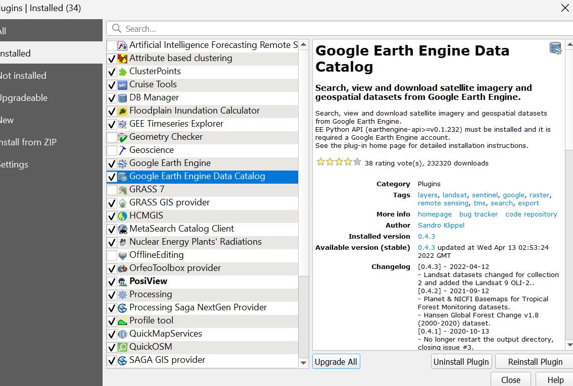
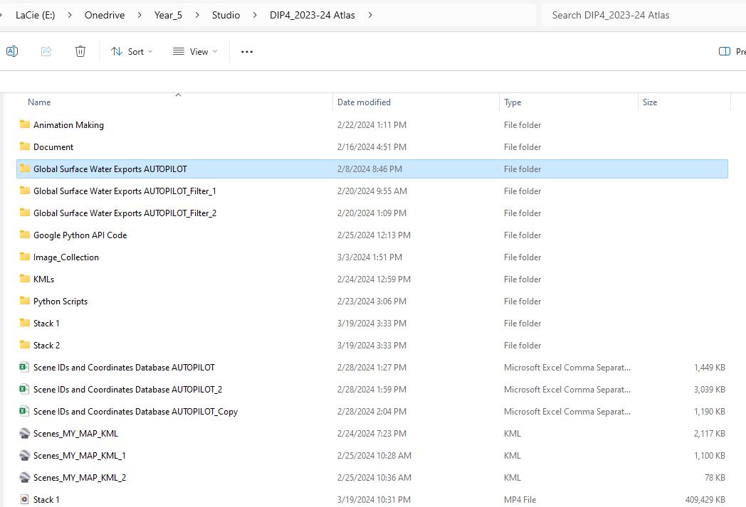
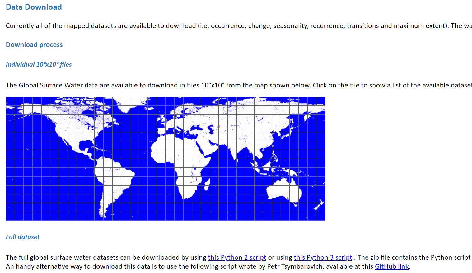
Step 1: Acquiring the Data

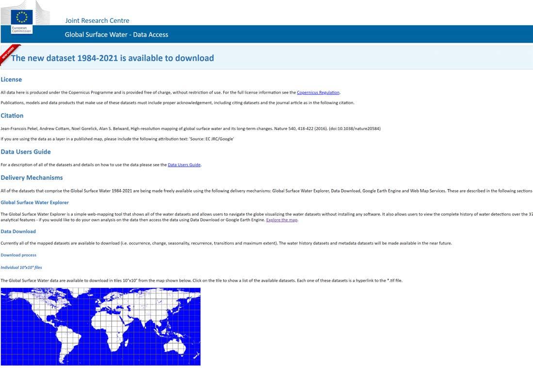
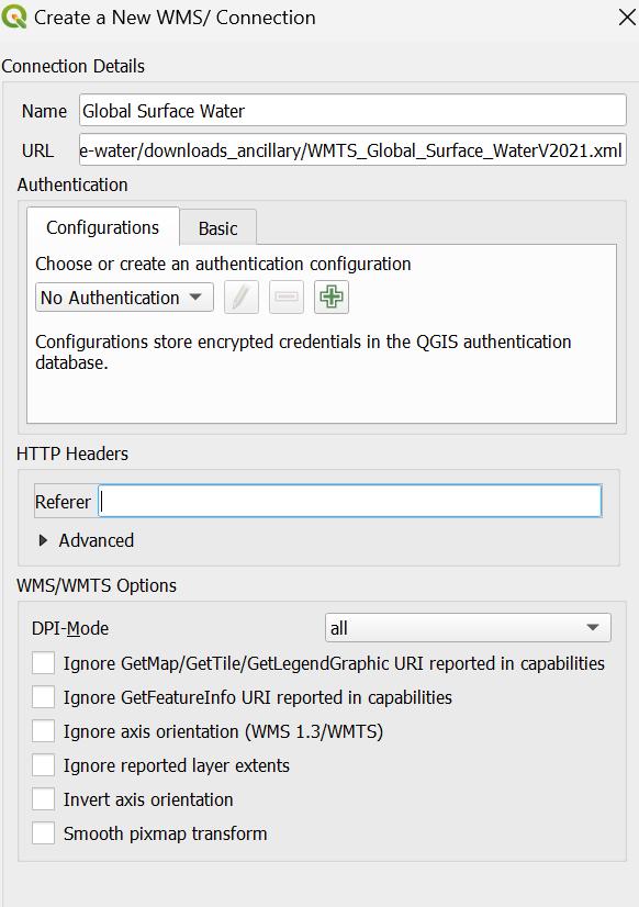
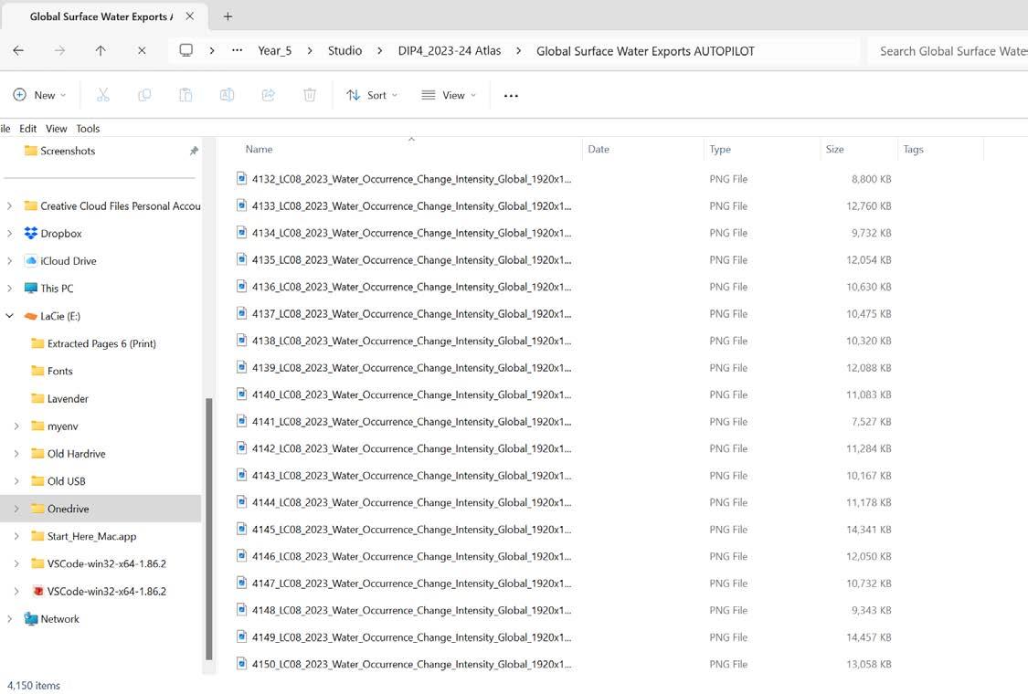
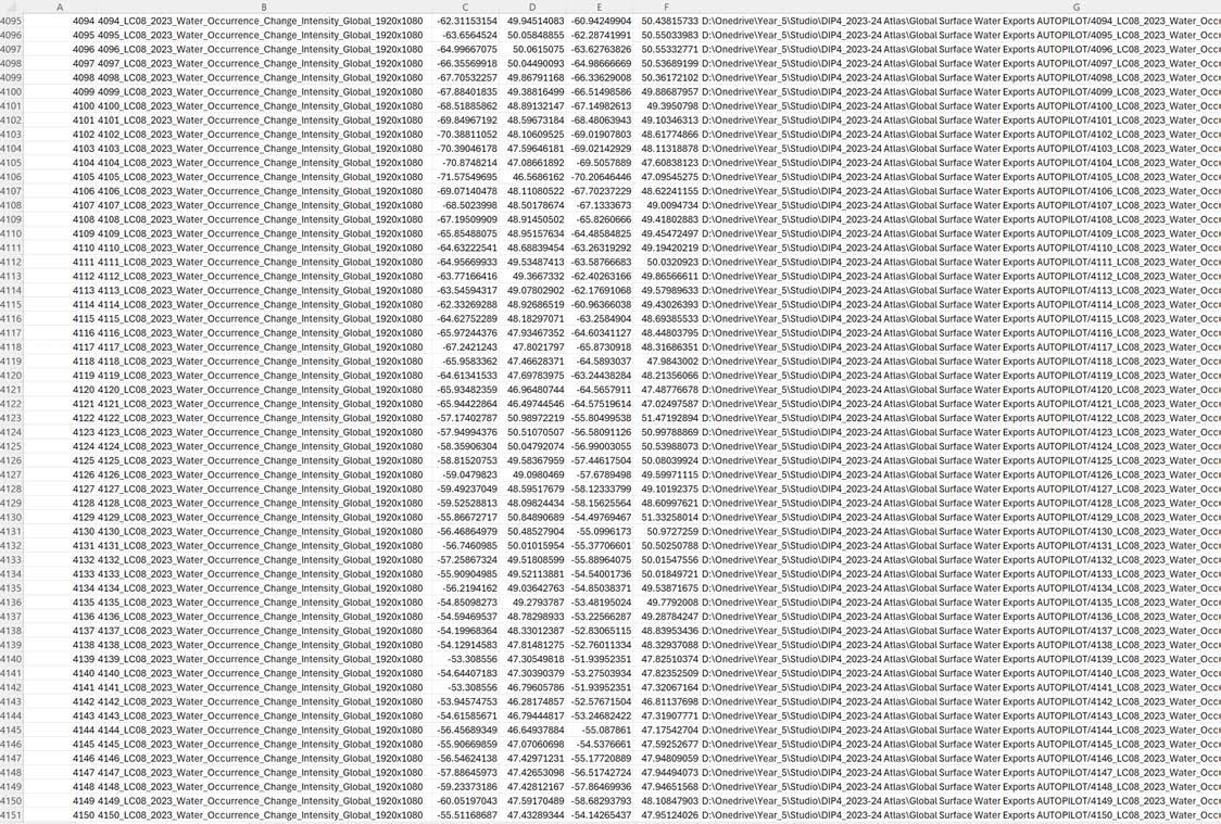
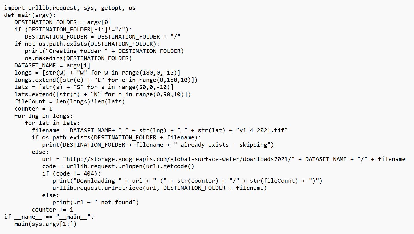
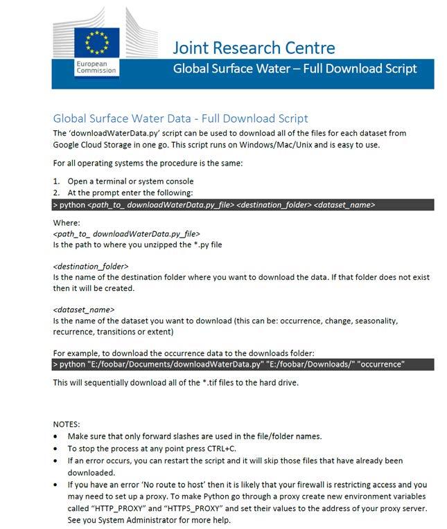
In the initial phase of the quantification process, a strategic shift is made in data acquisition to enable a detailed and comprehensive analysis. Step 1 introduces an automated approach to downloading geospatial data, utilizing a Python3 script made available by the European Commission’s Joint Research Centre.

The script facilitates the bulk downloading of individual data tiles, allowing for the subsequent automated pixel counting necessary for quantification. Each data tile, containing a staggering 40,000 by 40,000 pixels, represents a substantial amount of geographical information and, when aggregated, will form the basis for a detailed global analysis.

This method is crucial as it allows for consistent and unbiased access to the data across all regions, maintaining the integrity of the quantification process. By automating this step, the potential for human error is minimized, and the efficiency of the process is significantly enhanced. The script’s ability to interact seamlessly with the Global Surface Water dataset ensures that all available data for the chosen timeframe is included in the analysis, thereby ensuring that no area of interest is omitted due to manual oversight.

The use of this script sets the stage for an accurate

pixel-based analysis of the water occurrence changes. By methodically capturing the dataset in this manner, it provides the necessary granularity to detect and measure both the overt and subtle changes in water presence, which, in turn, will reflect the corresponding material flux. The downloaded data will serve as a foundational resource for the algorithms that will calculate the extent of coastal change by assessing the variations represented within each pixel. This step is pivotal for preparing the data for the rigorous computational processes that will follow in the quantification of global coastal extension.

Fig. 95. Download page where to obtain the individual tiles from. ©Global Surface Water

Fig. 96. The Python3 Code to install all tiles automatically. ©Global Surface Water

Fig. 97. Download instructions for the Python3 Code. ©Global Surface Water

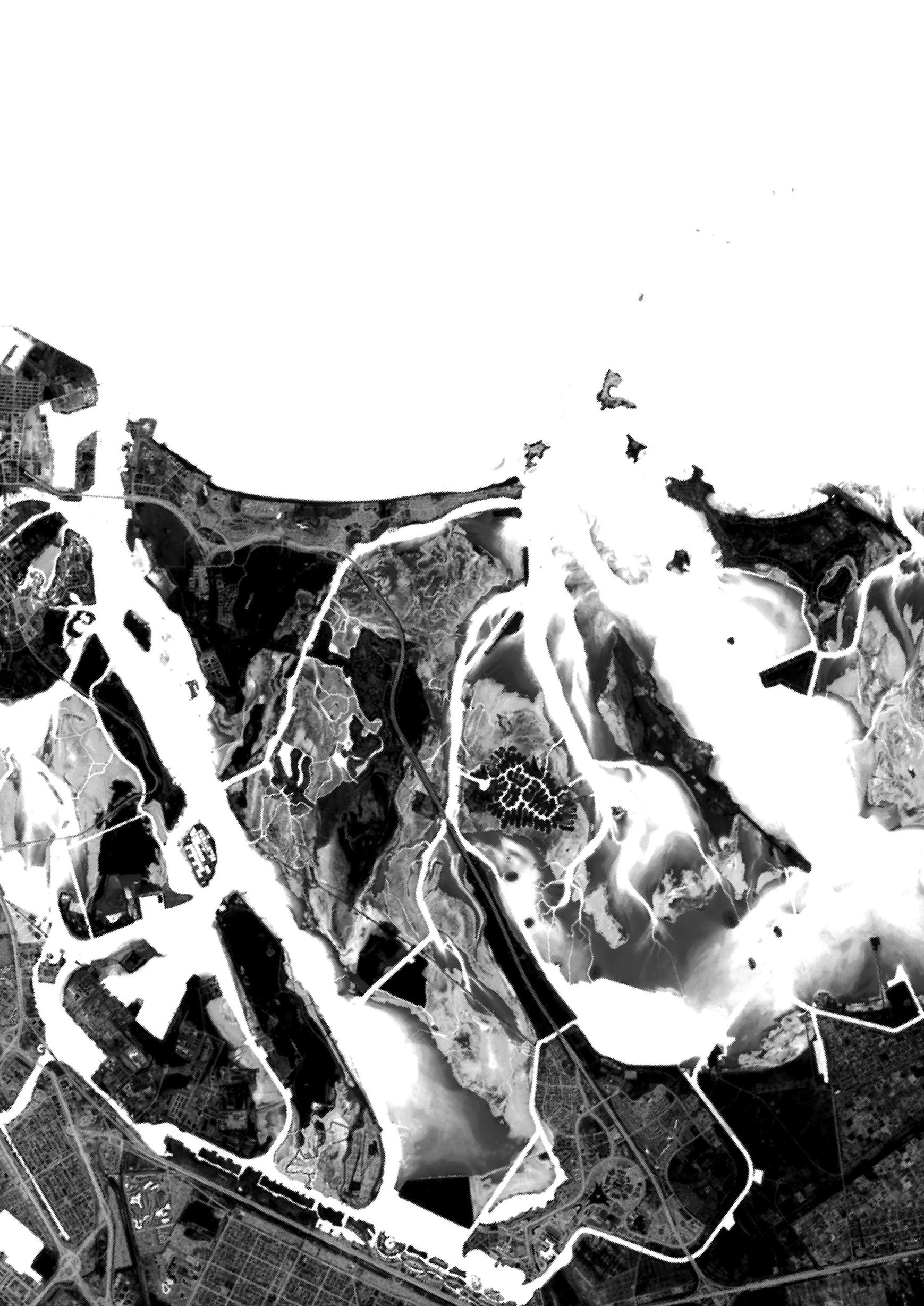
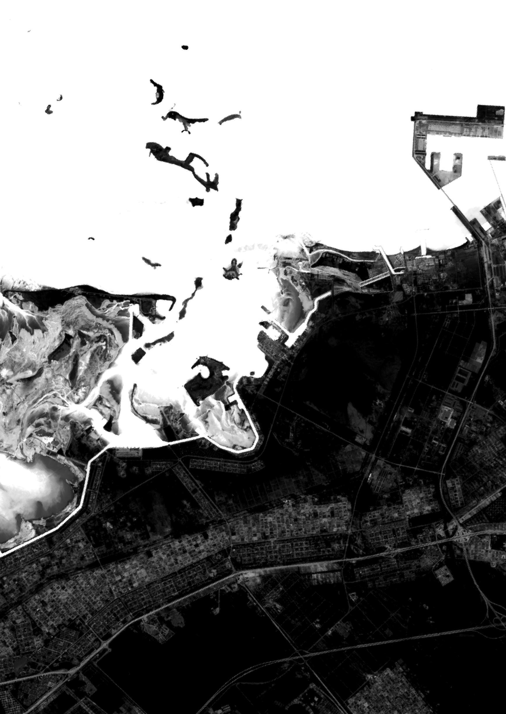
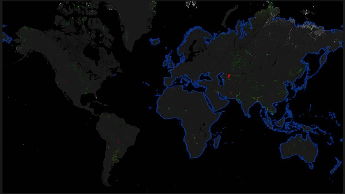
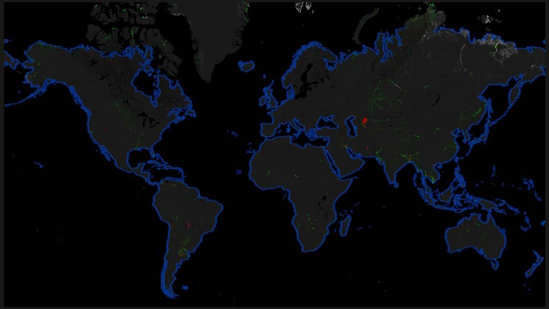
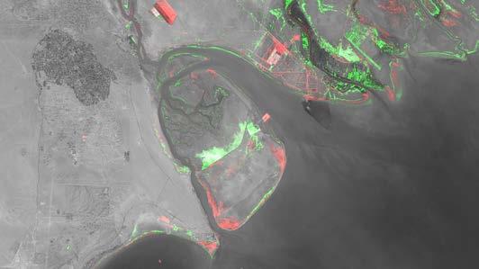
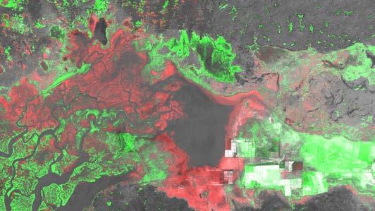
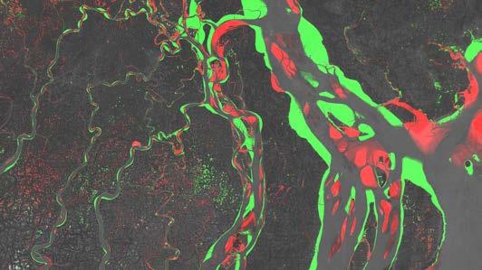
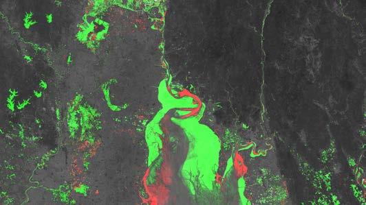
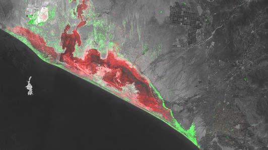
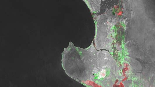
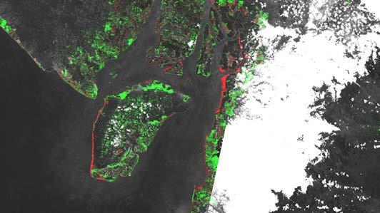
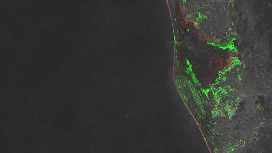
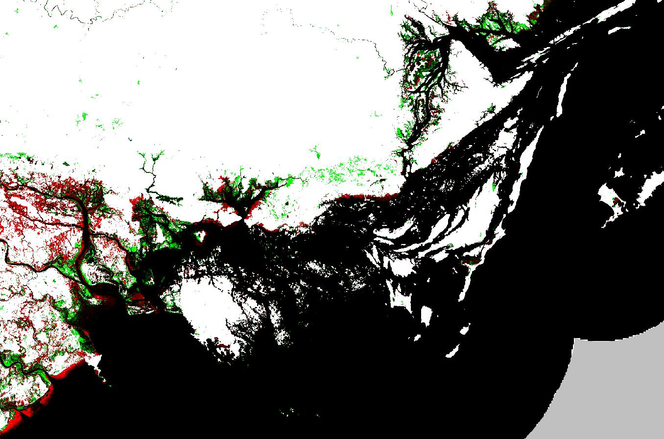
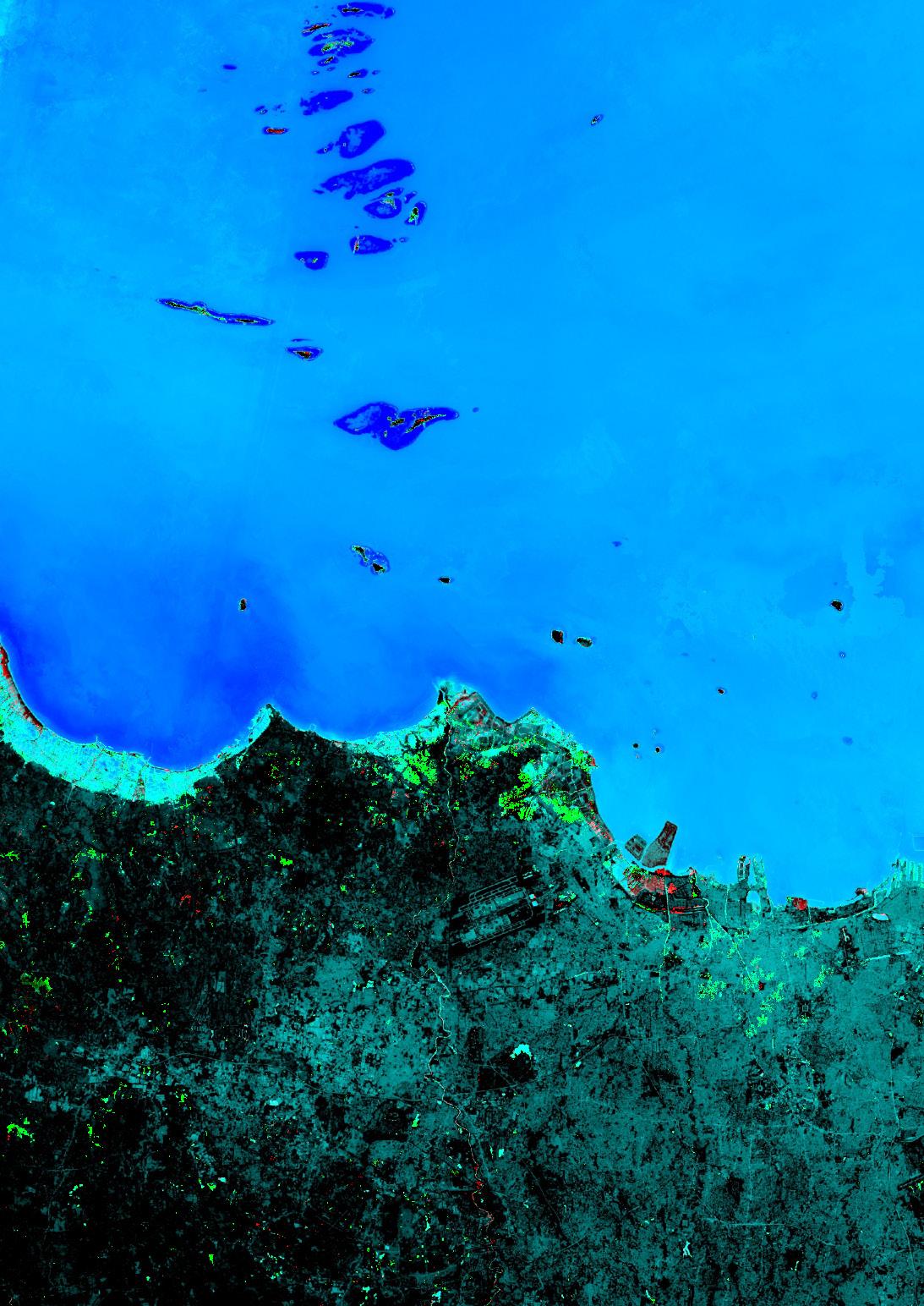
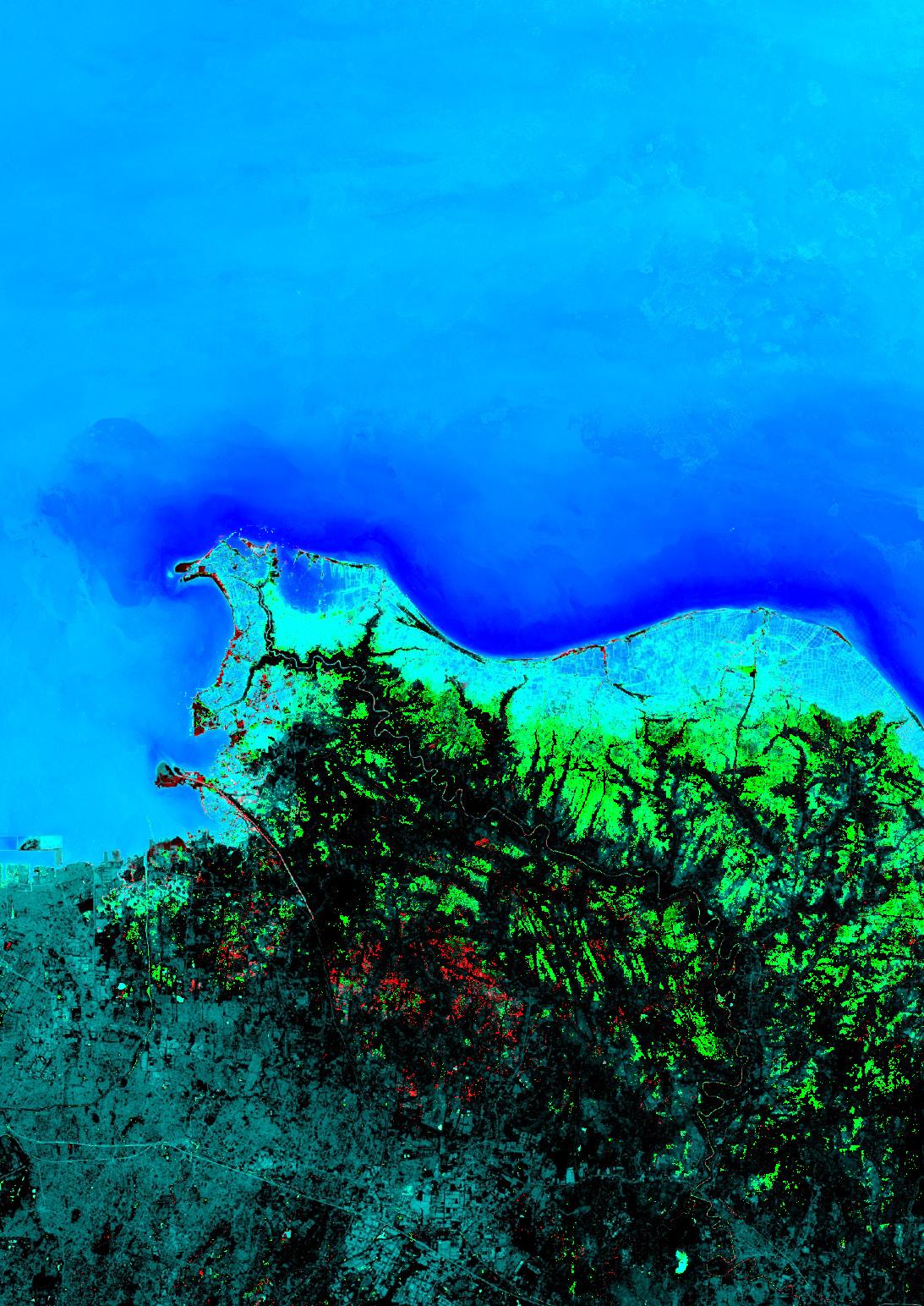
Step 2: Decoding Pixel Data

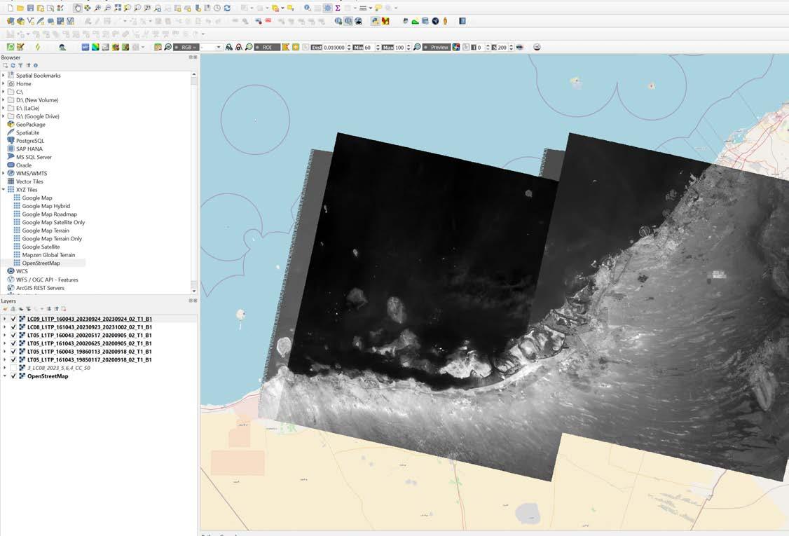
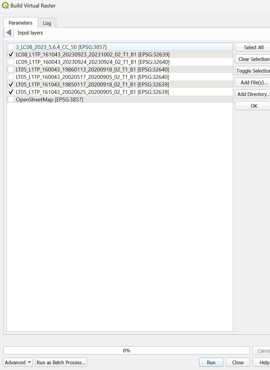
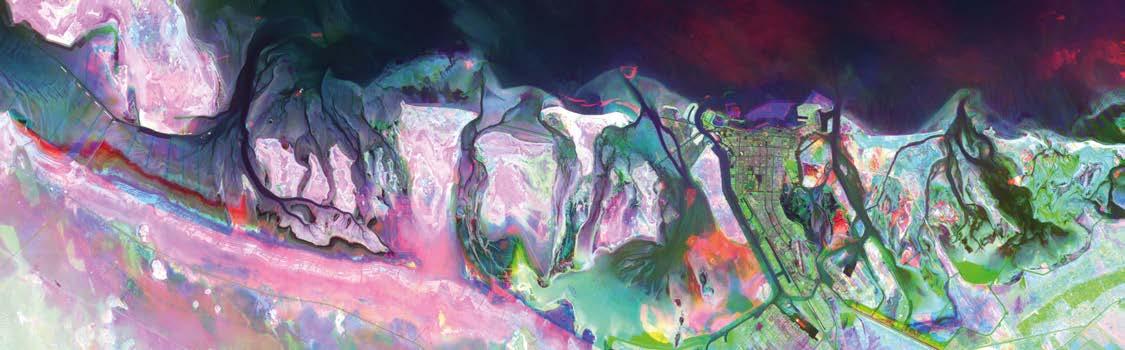
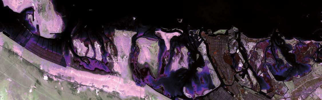
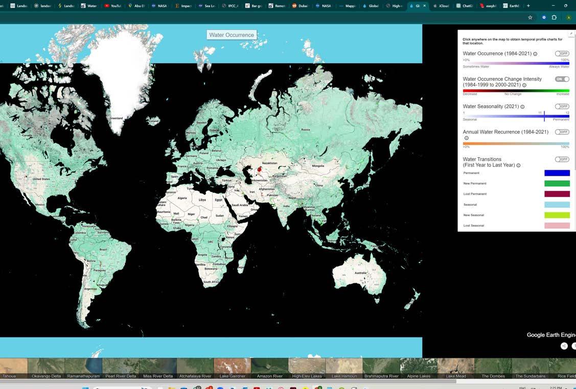
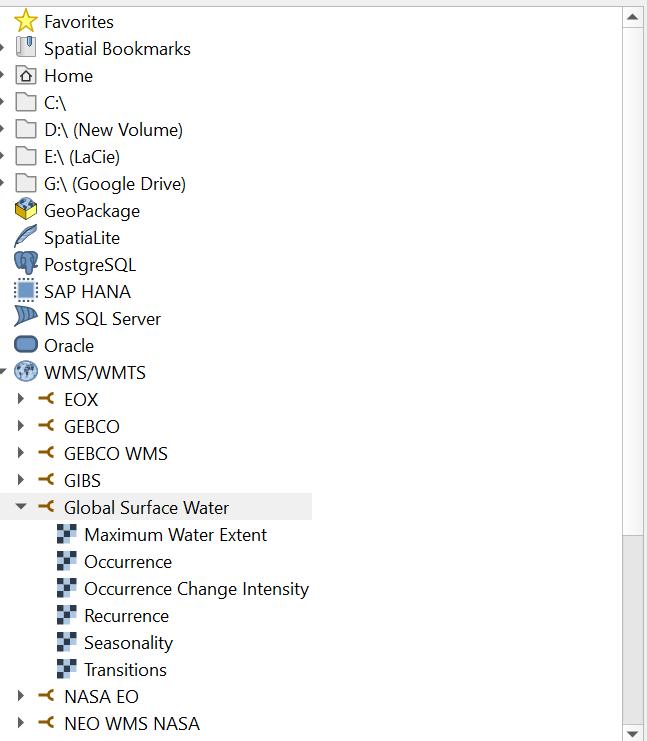
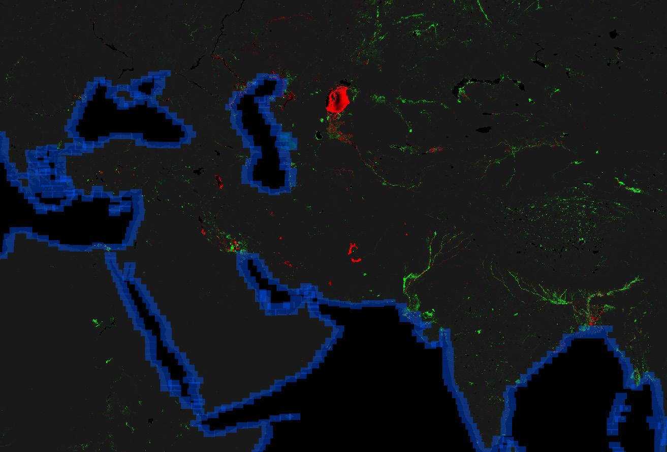
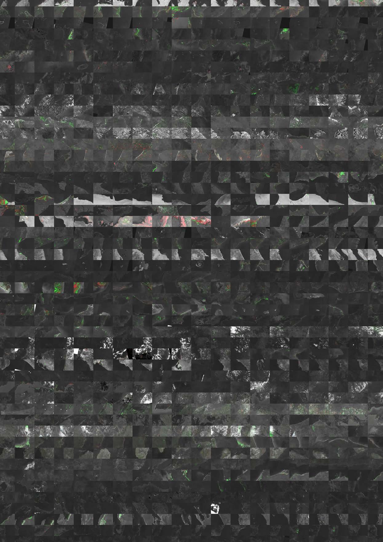
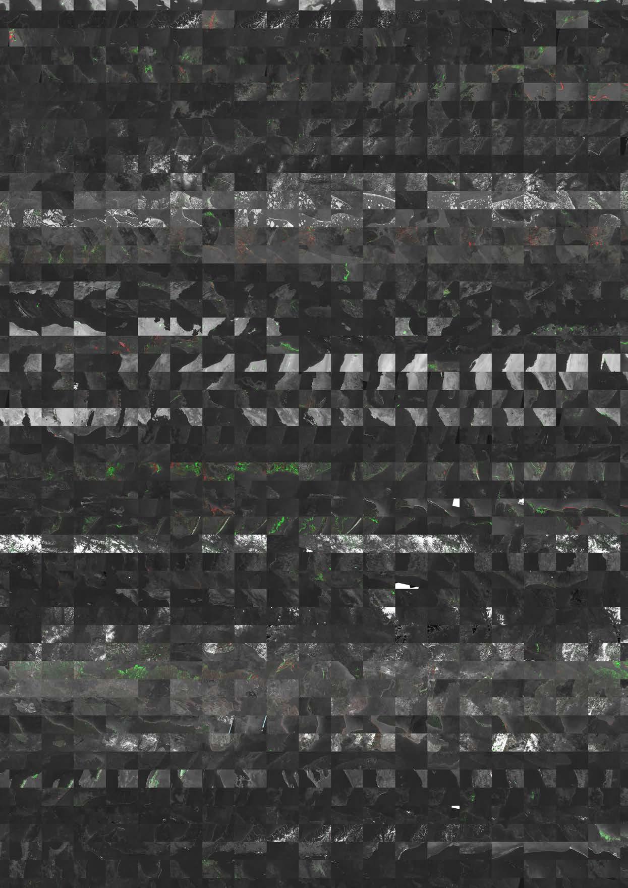
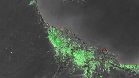
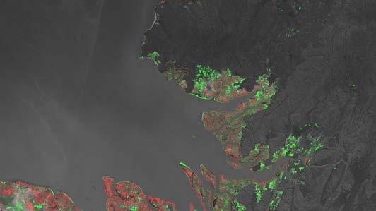
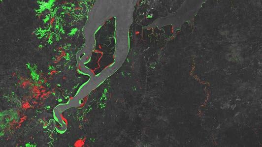
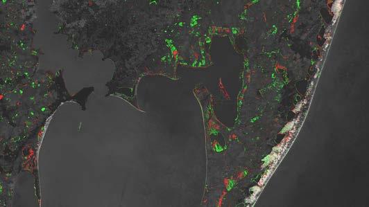
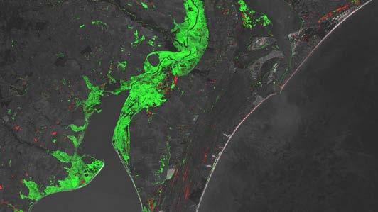
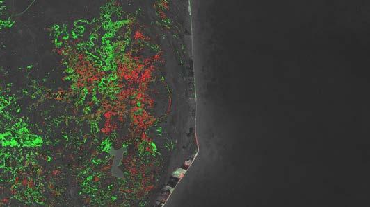
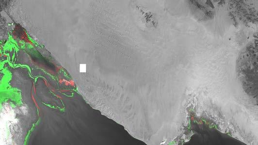
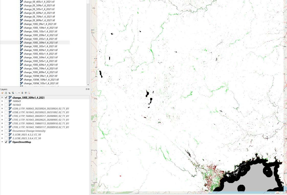
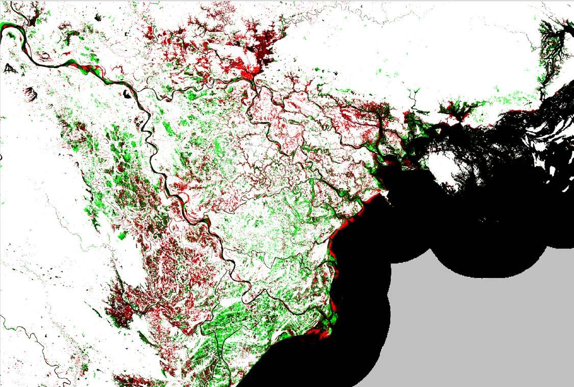
In Step 2 of the quantification process, the focus is on interpreting the rich tapestry of data encoded within each pixel of the global surface water tiles. To decode this vast array of information, a single tile is carefully selected and inspected within the QGIS platform, serving as a representative sample of the larger dataset.

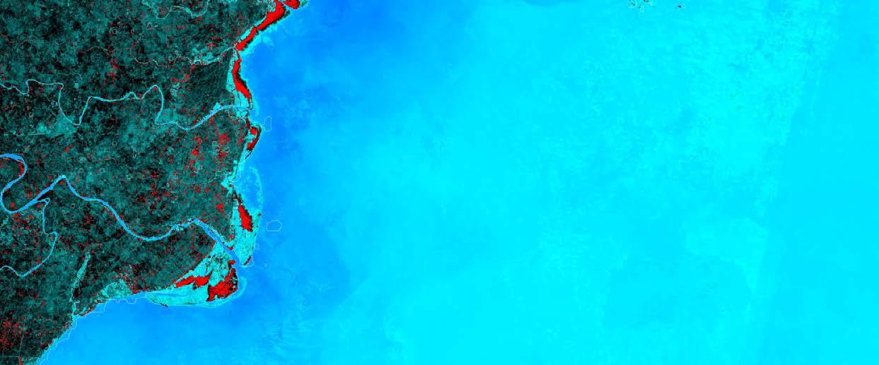
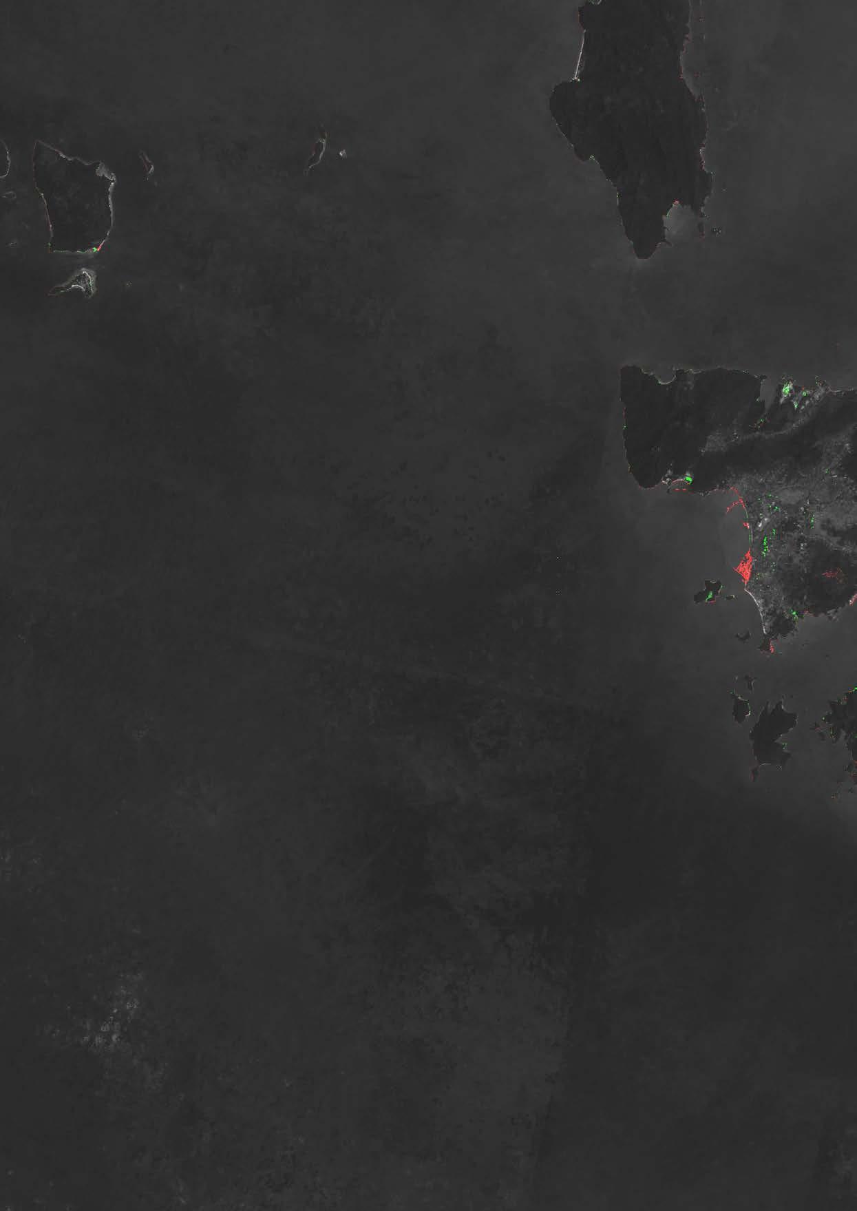
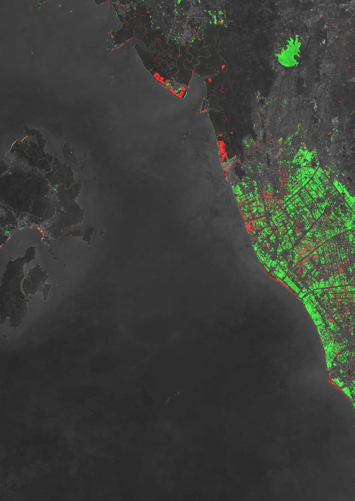
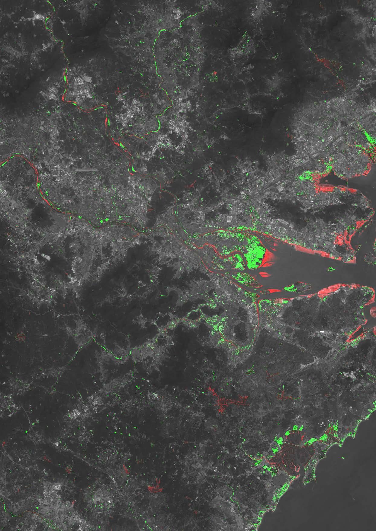
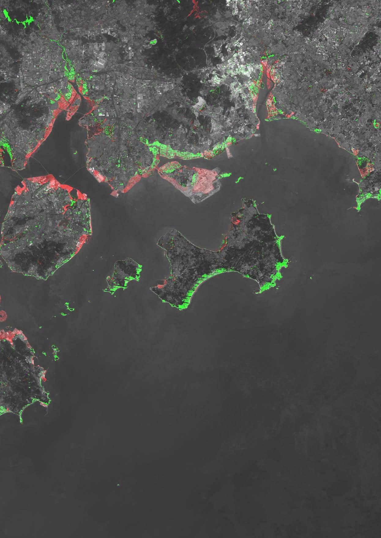
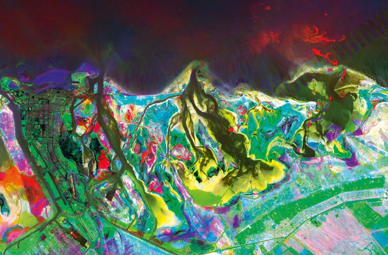
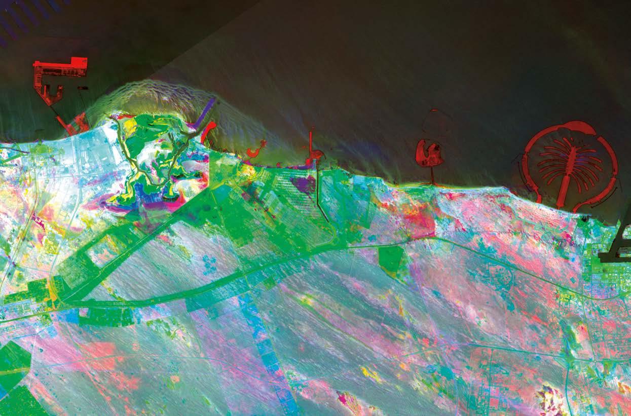
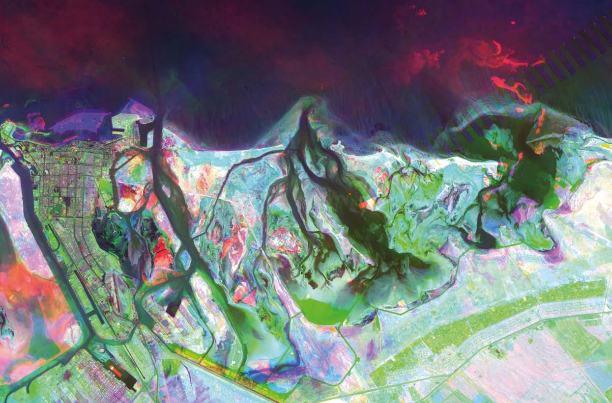
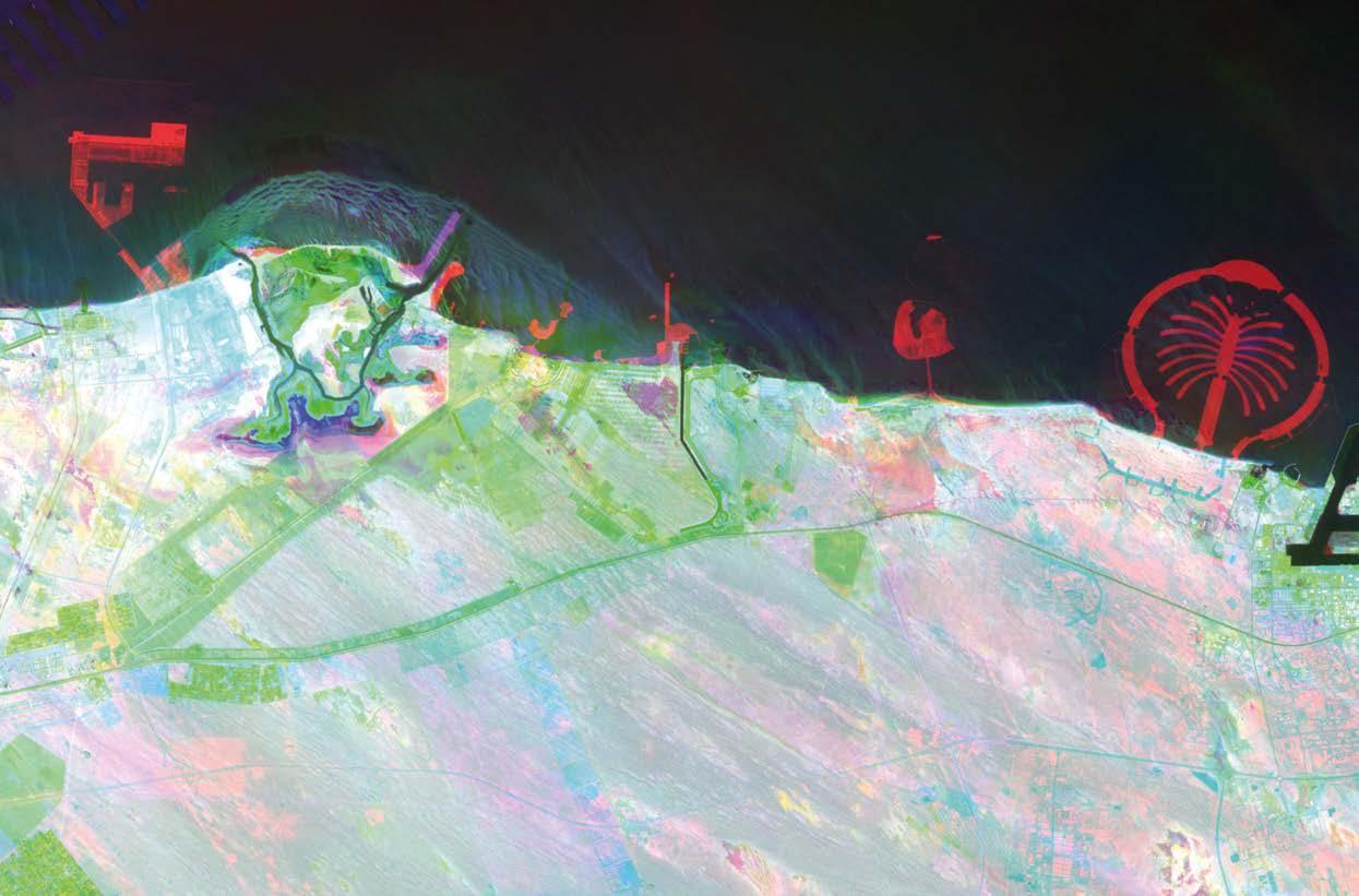
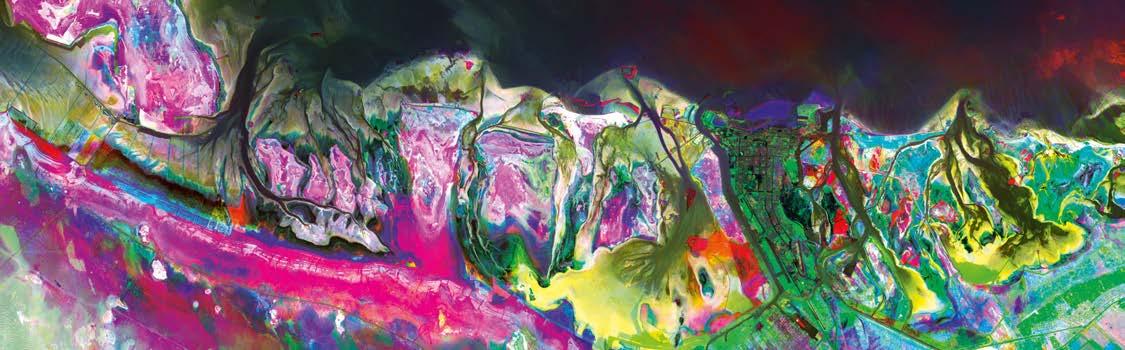
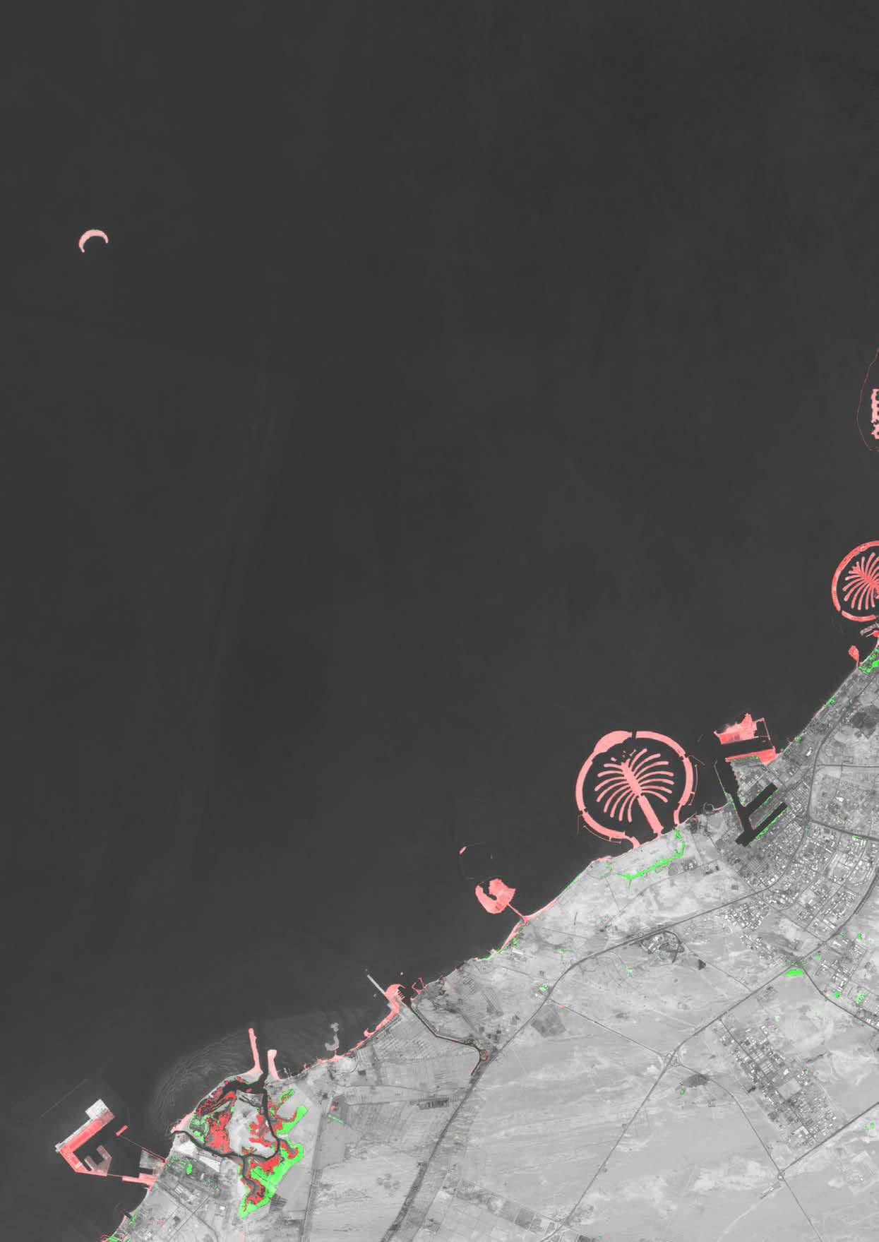
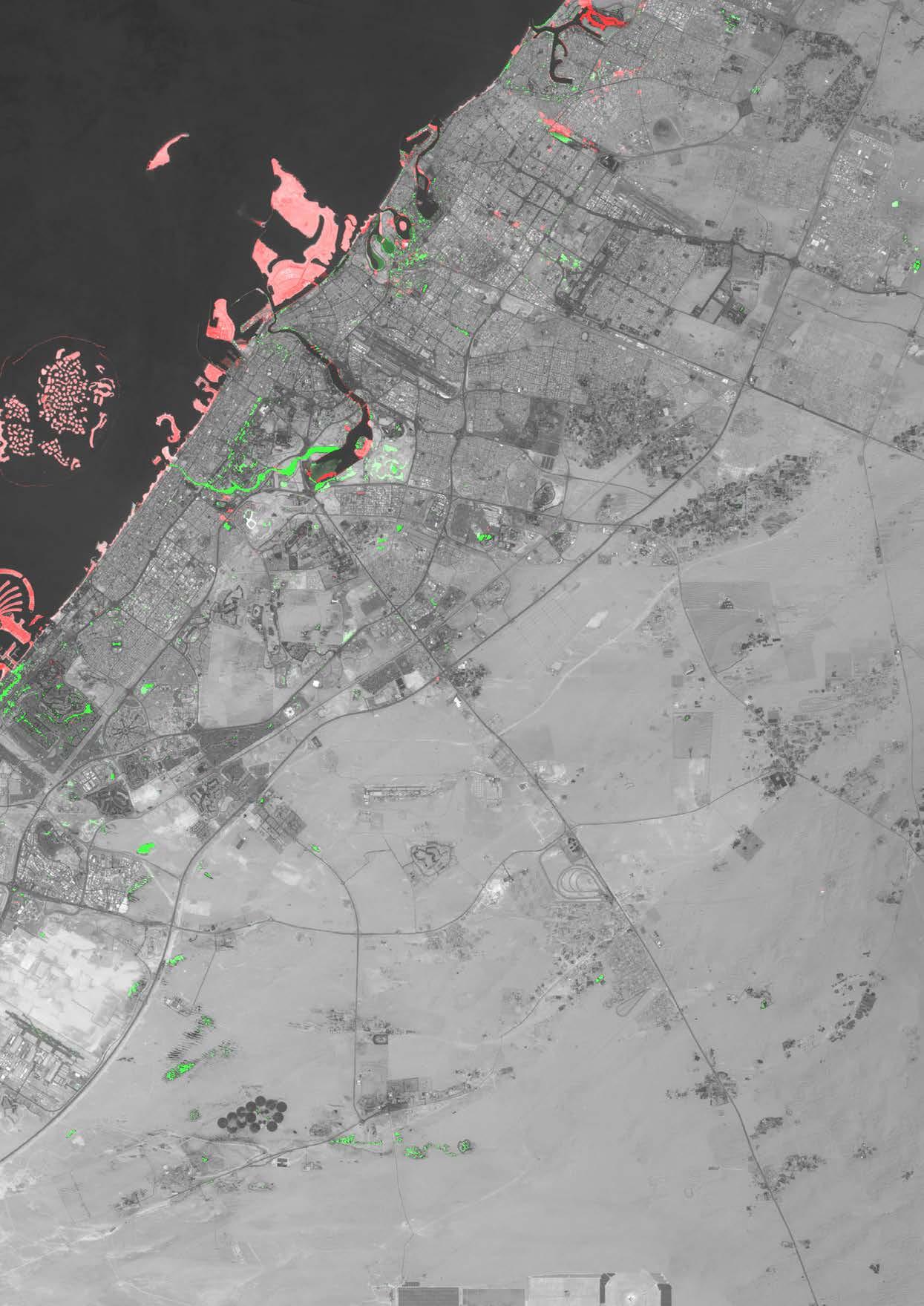
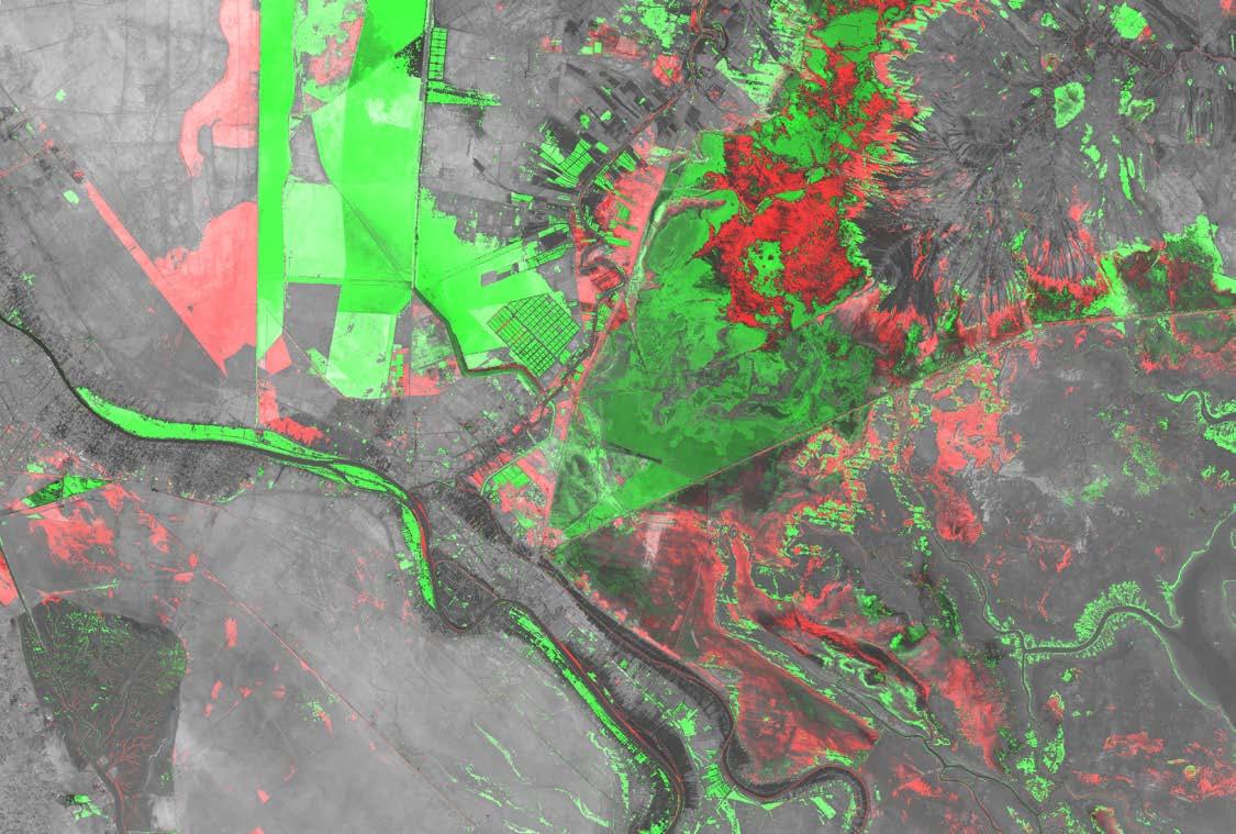
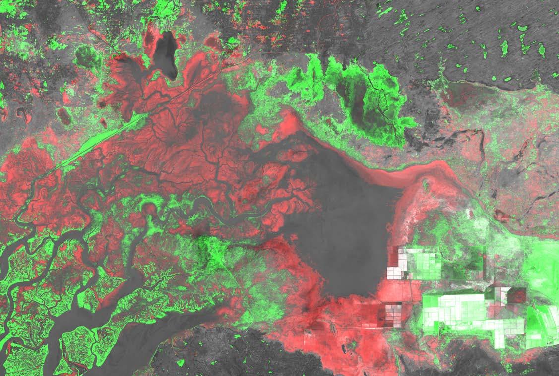
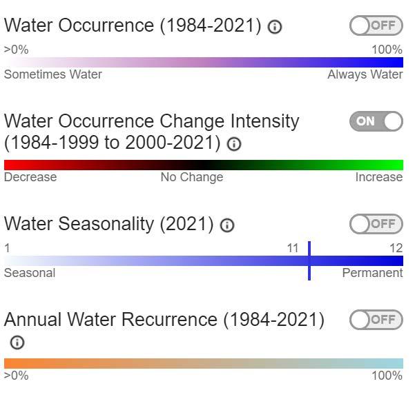
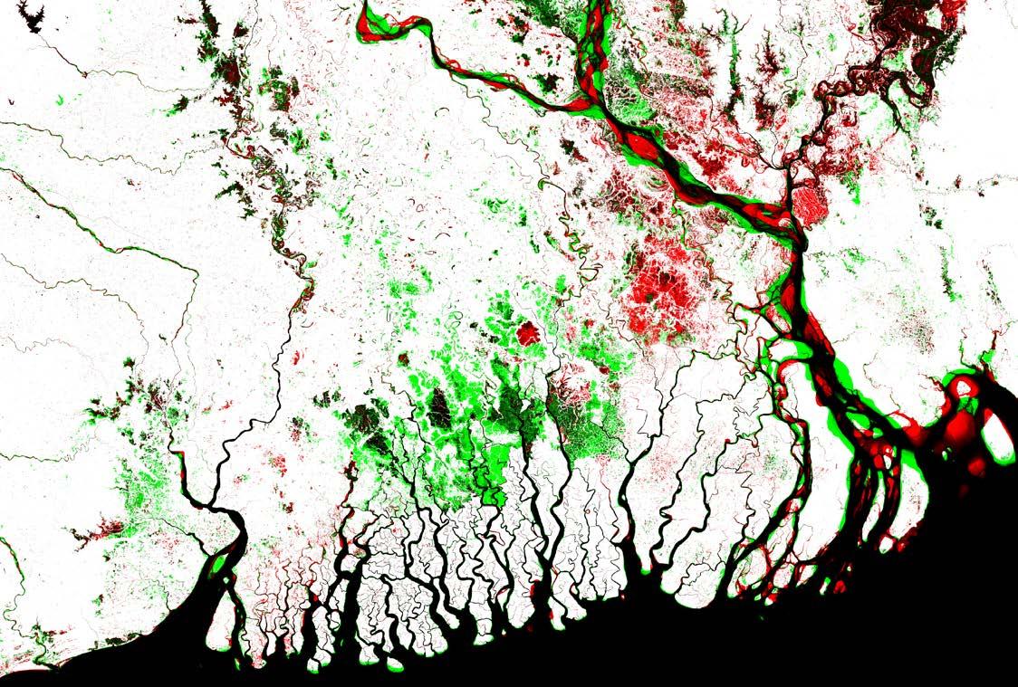
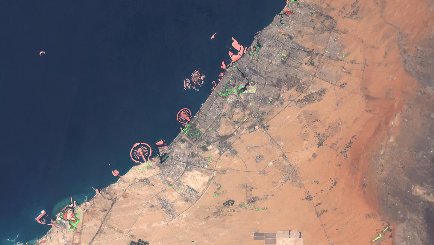
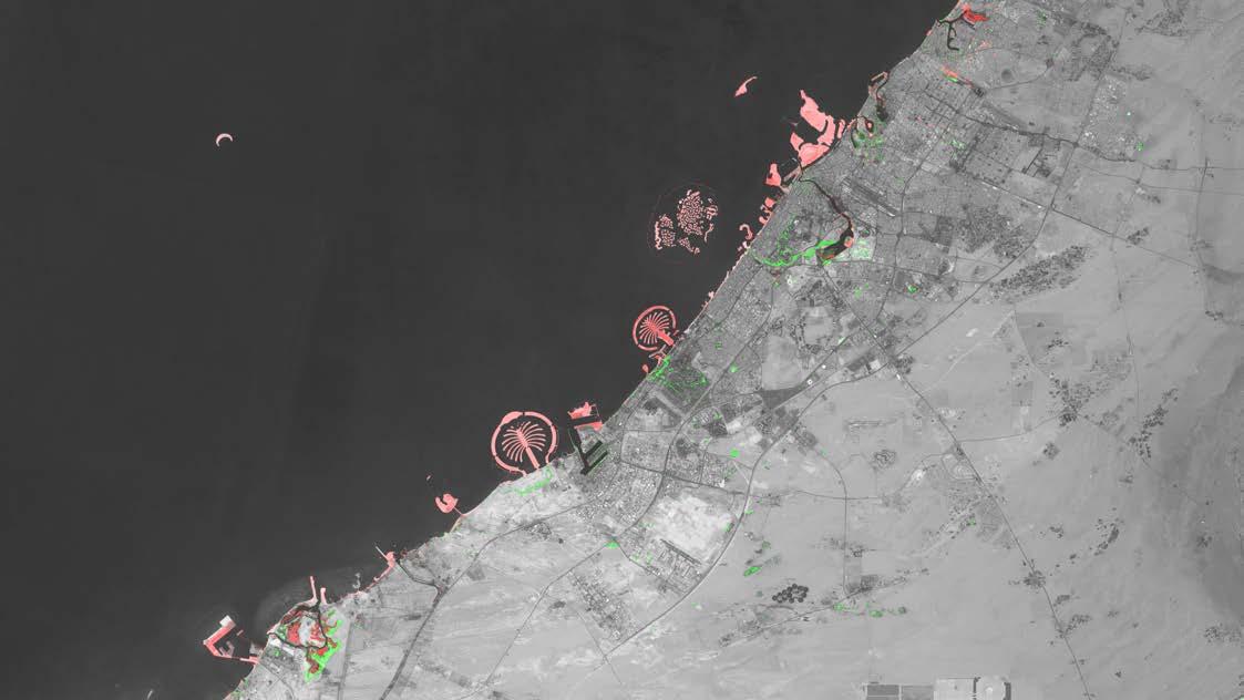
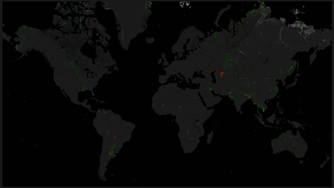
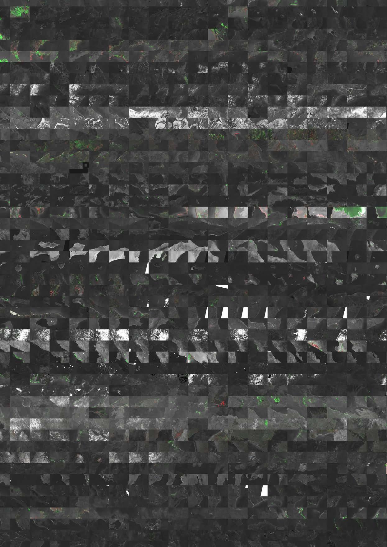
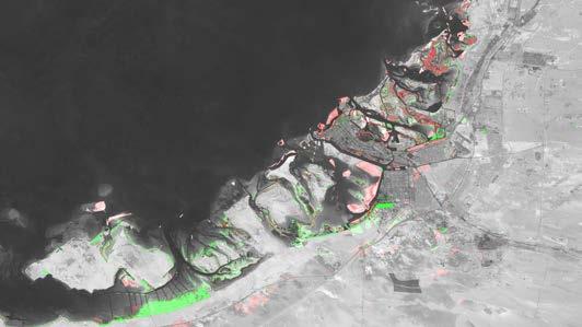
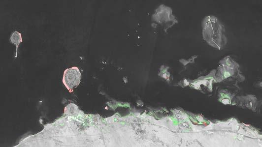
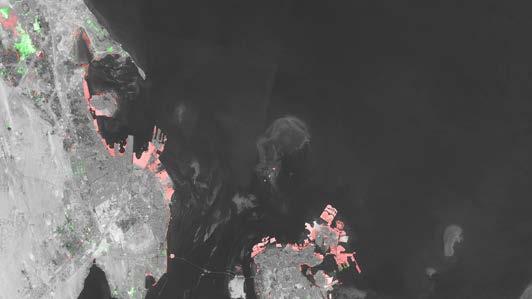
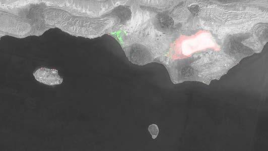
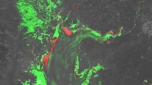
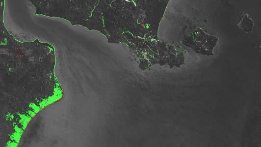
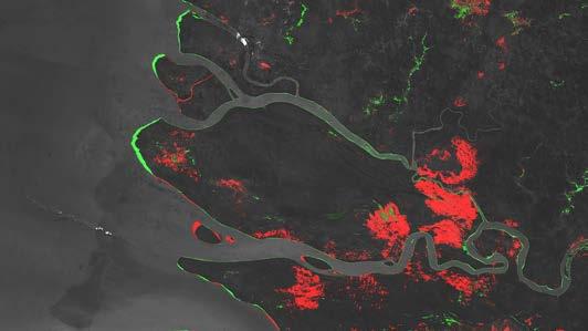
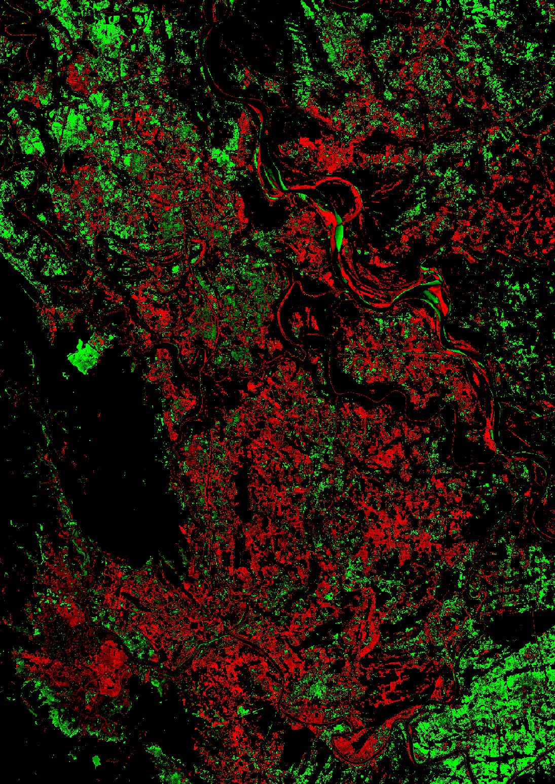
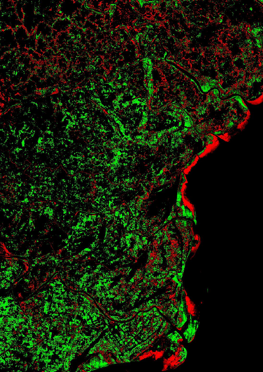
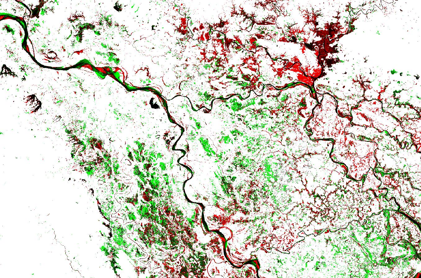
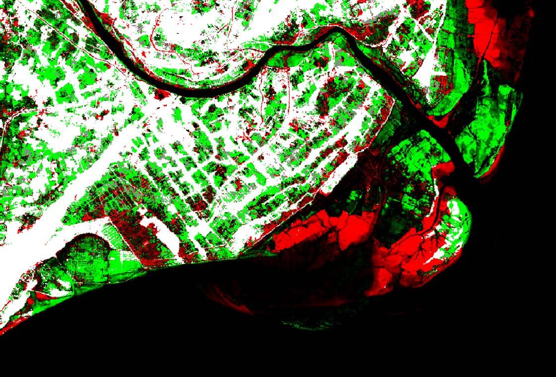
Upon examination of the layer properties, a diverse color palette is revealed, each shade corresponding to a distinct pixel value. This color code serves as a key, unlocking the narrative of water occurrence across the globe. The palette’s spectrum, ranging from greens to reds, visually represents the varying intensities of water presence changes over time—the greens signaling areas where water presence has increased, while the reds denote areas of decreased water presence.

The intensities of these colors bear significance, offering a graduated scale that reflects the magnitude of change. These variances are pivotal, as they inform the degree to which each region has experienced shifts in water coverage, directly impacting the material flux of coastal landscapes.

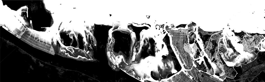
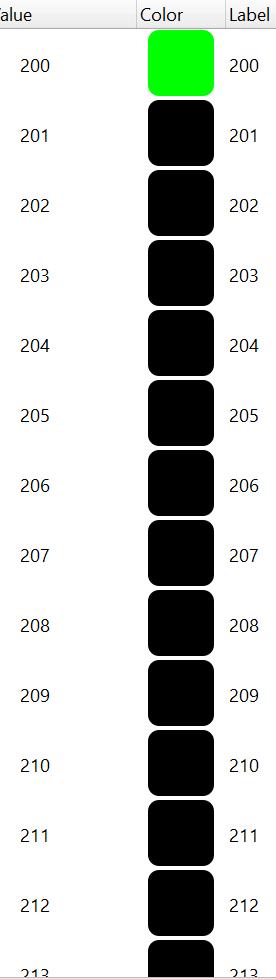
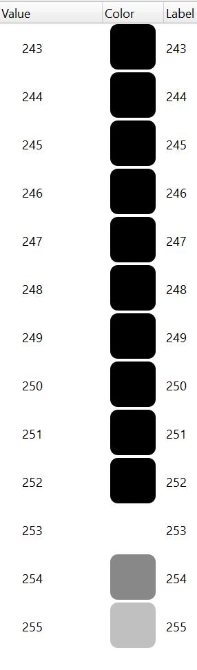
Crucially, black, white, and grey pixels denote absence of data or null values, and thus, are extraneous to the quantification endeavor. They must be diligently filtered out to refine the analysis and concentrate solely on the meaningful changes depicted by the vibrant hues. This meticulous sifting is imperative for achieving an accurate, data-driven portrayal of global

coastal dynamics—a task that sets the groundwork for the complex computation processes ahead. The elimination of these neutral pixels ensures the purity of the dataset, allowing the ensuing steps to calculate a precise measure of global material flux.

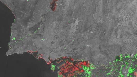
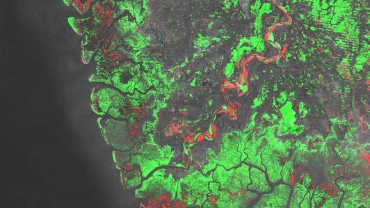
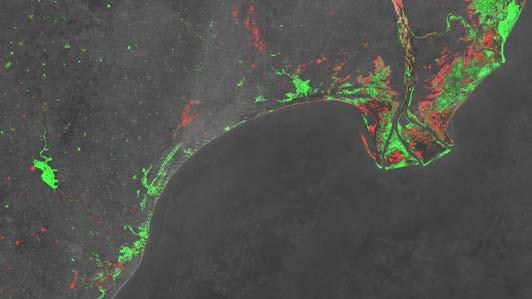
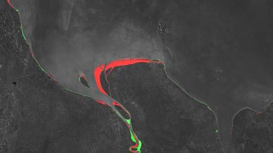
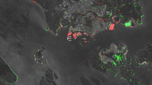
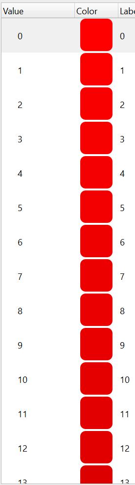
Step 3: Identifying the Correct Pixel Ranges

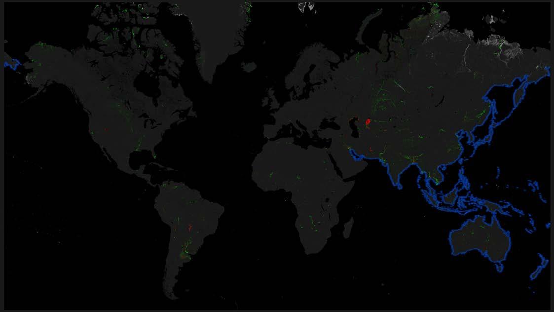
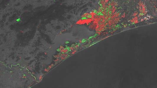
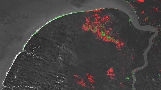
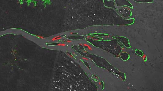
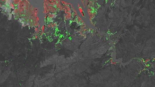
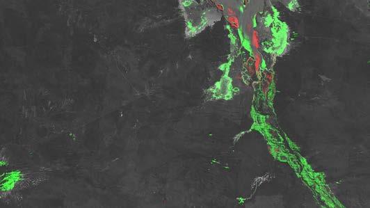
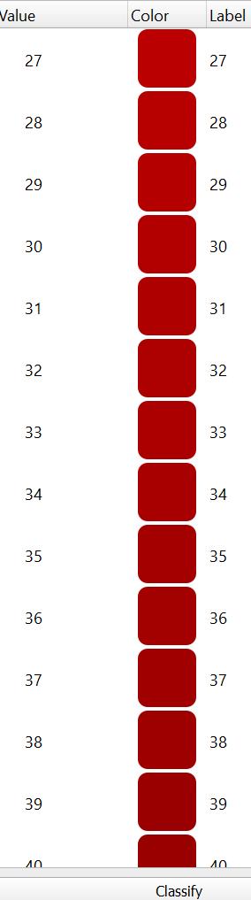
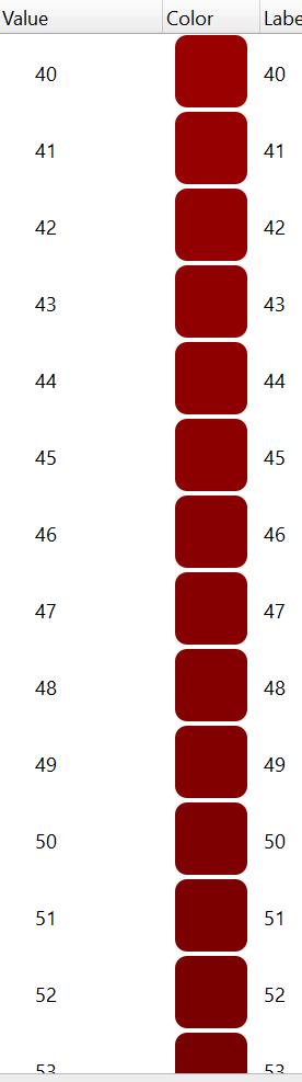
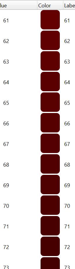
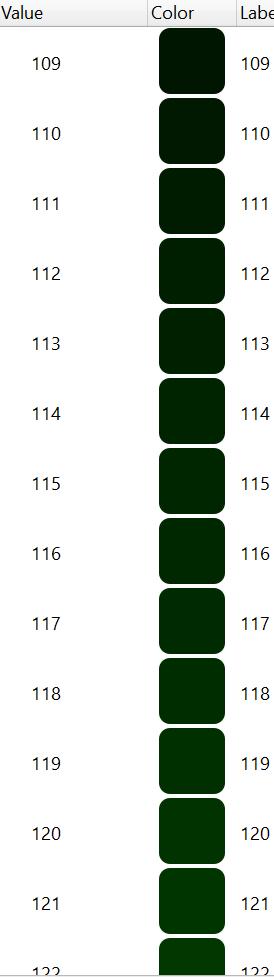
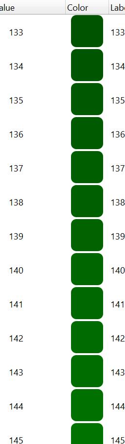
In step 3, the focus shifts to identifying the range of pixel values that correspond to significant changes in water occurrence. The color ramps illustrate a gradient of change, with each color representing a quantifiable alteration in water presence. The red end of the spectrum signals a reduction in water occurrence, whereas the green indicates an increase.

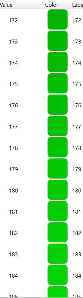
The progression of the color ramps seen on the right side of the page on the right demonstrates the intensity of water occurrence change. The darker shades of red, nearing the black mid-point, represent areas with the most significant reduction in water presence over time. Conversely, the brighter shades of green, approaching the white end, signify regions where water occurrence has increased markedly.

For precise quantification, a buffer zone is considered to accommodate the ambiguity of moderate changes that are closer to the mid-point, which is represented by black (value 100). Red values ranging from 0-75 encapsulate a marked decrease in water occurrence, including a buffer zone to ensure that even less intense but still significant decreases are accounted for. Similarly, green values from 125-200 are chosen to represent an increase in water occurrence, excluding the immediate vicinity of the neutral black value to focus on more pronounced changes.

This meticulous selection ensures that only those changes that are most discernible and consequential are included in the quantification, thus prioritizing

alterations that are not only visible to the eye but are also substantial enough to indicate significant material flux. It’s a targeted approach to quantify the magnitude of change, giving precedence to the most striking shifts that define the dynamics of coastal extensions and retreats.

Fig. 98. The range of reds that indicates different intensities of change.

Fig. 99. The range of greens that indicates different intensities of change.

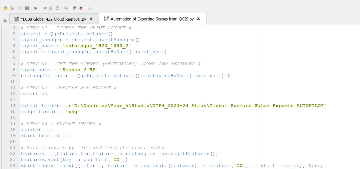
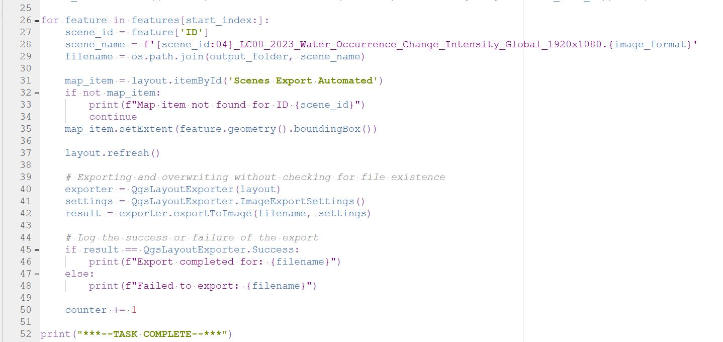
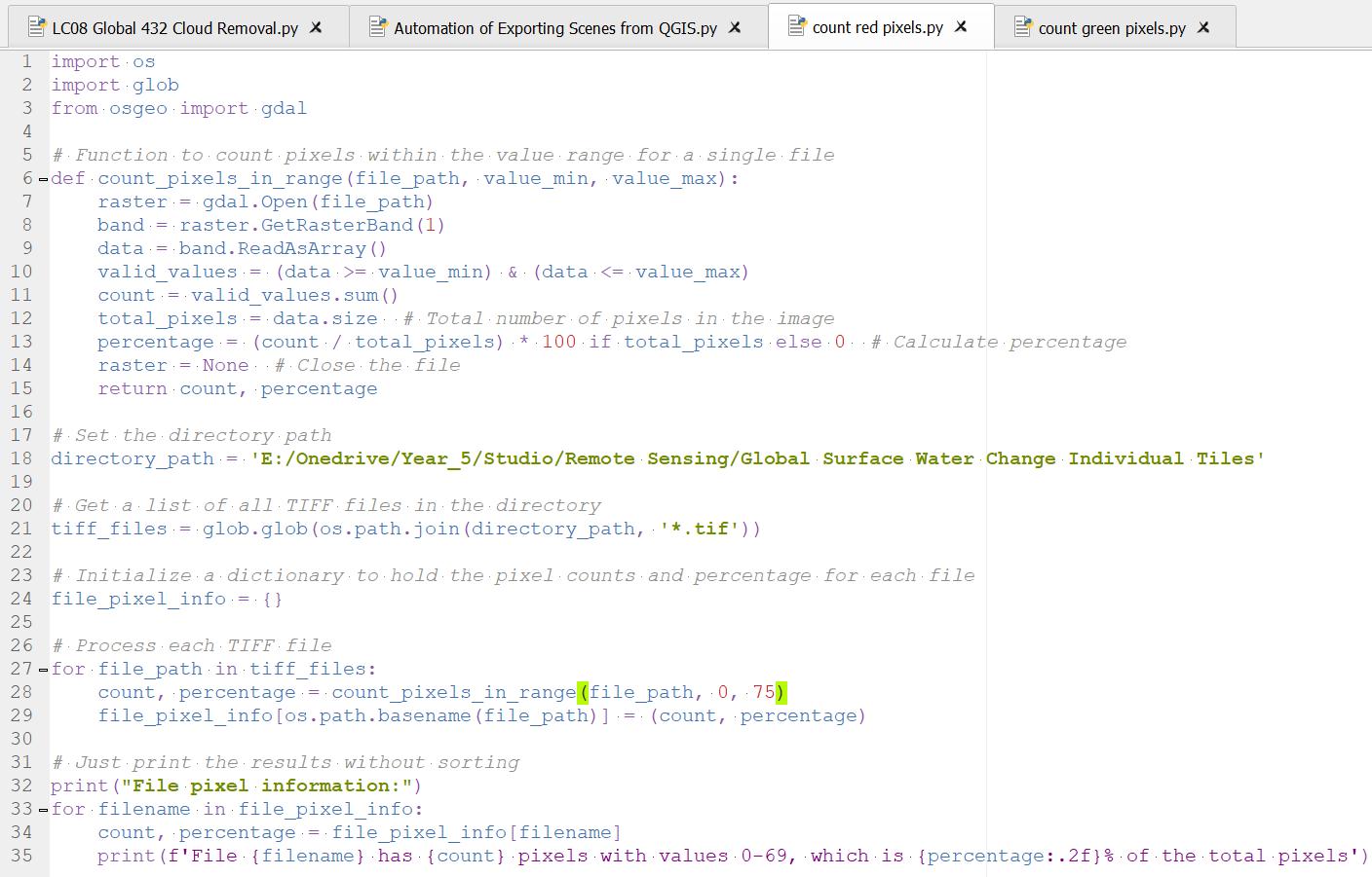
Step 4: Code Writing to Obtain Total Red Pixel Count

Scripting an automated process to tally the number of pixels within a specified value range that represents areas with decreased water occurrence, applying a function that counts and computes the percentage of pixels with values that fall between 0 and 75.

These pixel values are quantified for each image, and the total is accumulated, thus providing a comprehensive measure of the extent and intensity of water reduction across the global coastal regions.

Breakdown:

1. Imports:

- `os`: Provides a way of using operating system dependent functionality.

- `glob`: Finds all the pathnames matching a specified pattern according to the rules used by the Unix shell.

- `gdal`: Open source Geospatial Data Abstraction Library, for reading and writing raster and vector geospatial data formats.

2. Function Definition:

- `count_pixels_in_range(file_path, value_min, value_max)`: A function that counts the pixels within the specified range of values (value_min to value_max) in a single image file.

3. Opening the Raster:

- `gdal.Open(file_path)`: Opens the image file.

- `GetRasterBand(1)`: Fetches the first band of the raster image since we are assuming a single band with relevant data.

4. Processing the Data:

- `ReadAsArray()`: Reads the band’s data as an array for processing.

- `valid_values = (data >= value_min) & (data <= value_max)`: Creates a boolean array where true values correspond to pixels within the specified range.

- `count = valid_values.sum()`: Sums the boolean array to get the count of valid pixels.

- `total_pixels = data.size`: Gets the total number of pixels in the image.

- `percentage = (count / total_pixels) * 100`: Calculates the percentage of pixels in the valid range.

5. Setting Directory and Processing Files:

- The script sets a directory path where the TIFF images are stored.

- It lists all the TIFF files in the directory using `glob. glob()`.

- Initializes a dictionary to hold the pixel count and percentage information for each image.

6. Iterating Over Images:

- For each image file, the script calls the `count_pixels_in_range()` function with the defined value range and adds the results to the dictionary.

7. Output:

- It prints out the file name along with the count of pixels in the specified range and the percentage this count represents of the total pixels.

Step 5: Code Writing to Obtain Total Green Pixel Count

Counterpoint to the previous red pixel count, focusing on areas with increased water occurrence.

The process involves a Python script that sifts through each image file, counting pixels in the value range of 125 to 200. These values signify the regions with more water presence over time, reflecting potential expansion of water bodies or flooding.

The green pixels represent not just water, but the movement and addition of material in the landscape, thus directly contributing to the global material flux. This script ensures that each green pixel is accounted for, painting a detailed picture of where and to what extent material deposition has occurred.

Breakdown:

1. Import Modules:

- `os`: To interact with the operating system.

- `glob`: To find all the pathnames matching a specified pattern.

- `gdal`: To handle raster data.

2. Function Definition – count_pixels_in_range():

- This function opens a TIFF file and counts pixels within a specified value range, intended for identifying pixels representing increased water occurrence (the green pixels in the dataset).

3. Open Raster File:

- The TIFF file is opened using `gdal.Open()` and the first band is selected since the TIFF files are assumed to contain a single band of data.

4. Read Data and Count Pixels:

- The `ReadAsArray()` function reads the band’s data as an array.

- It then identifies valid pixels in the specified range (125 to 200 in this case, representing the green pixel values for increased water occurrence).

- The total count of valid pixels is calculated, and its percentage against the total pixels in the image is determined.

5. Prepare for Output:

- The path to the directory containing the TIFF files is defined.

- A list of TIFF files is generated using the `glob. glob()` function.

- A dictionary is initialized to hold the count and percentage of pixels that match the criteria for each file.

6. Iterate Over Each TIFF File:

- The script loops through each TIFF file, calling the `count_pixels_in_range()` function, and populates the dictionary with the filename as the key and a tuple of the count and percentage as the value.

7. Display Results:

- Finally, the script prints out the pixel information without sorting, displaying the filename along with the count of green pixels and the percentage of the total pixels they represent.

6.3 Results

Red Pixels Count:

File change_180W_50Sv1_4_2021.tif has 0 pixels with values 0-75, which is 0.00% of the total pixels

File change_180W_40Sv1_4_2021.tif has 282 pixels with values 0-75, which is 0.00% of the total pixels

File change_180W_30Sv1_4_2021.tif has 0 pixels with values 0-75, which is 0.00% of the total pixels

File change_180W_20Sv1_4_2021.tif has 63961 pixels with values 0-75, which is 0.00% of the total pixels

File change_180W_10Sv1_4_2021.tif has 4843 pixels with values 0-75, which is 0.00% of the total pixels

File change_180W_0Nv1_4_2021.tif has 112640 pixels with values 0-75, which is 0.01% of the total pixels

File change_180W_10Nv1_4_2021.tif has 0 pixels with values 0-75, which is 0.00% of the total pixels

File change_180W_20Nv1_4_2021.tif has 0 pixels with values 0-75, which is 0.00% of the total pixels

File change_180W_30Nv1_4_2021.tif has 0 pixels with values 0-75, which is 0.00% of the total pixels

File change_180W_40Nv1_4_2021.tif has 61440 pixels with values 0-75, which is 0.00% of the total pixels

File change_180W_50Nv1_4_2021.tif has 0 pixels with values 0-75, which is 0.00% of the total pixels

File change_180W_60Nv1_4_2021.tif has 60206 pixels with values 0-75, which is 0.00% of the total pixels

File change_180W_70Nv1_4_2021.tif has 701032 pixels with values 0-75, which is 0.04% of the total pixels

File change_180W_80Nv1_4_2021.tif has 0 pixels with values 0-75, which is 0.00% of the total pixels

Red Pixel Count: 942,964

Cumulative Pixel Count:

942,964

File change_170W_50Sv1_4_2021.tif has 0 pixels with values 0-75, which is 0.00% of the total pixels

File change_170W_40Sv1_4_2021.tif has 0 pixels with values 0-75, which is 0.00% of the total pixels

File change_170W_30Sv1_4_2021.tif has 0 pixels with values 0-75, which is 0.00% of the total pixels

File change_170W_20Sv1_4_2021.tif has 0 pixels with values 0-75, which is 0.00% of the total pixels

File change_170W_10Sv1_4_2021.tif has 0 pixels with values 0-75, which is 0.00% of the total pixels

File change_170W_0Nv1_4_2021.tif has 0 pixels with values 0-75, which is 0.00% of the total pixels

File change_170W_10Nv1_4_2021.tif has 0 pixels with values 0-75, which is 0.00% of the total pixels

File change_170W_20Nv1_4_2021.tif has 45056 pixels with values 0-75, which is 0.00% of the total pixels

File change_170W_30Nv1_4_2021.tif has 41482 pixels with values 0-75, which is 0.00% of the total pixels

File change_170W_40Nv1_4_2021.tif has 0 pixels with values 0-75, which is 0.00% of the total pixels

File change_170W_50Nv1_4_2021.tif has 0 pixels with values 0-75, which is 0.00% of the total pixels

File change_170W_60Nv1_4_2021.tif has 140205 pixels with values 0-75, which is 0.01% of the total pixels

File change_170W_70Nv1_4_2021.tif has 3500508 pixels with values 0-75, which is 0.22% of the total pixels

File change_170W_80Nv1_4_2021.tif has 79028 pixels with values 0-75, which is 0.00% of the total pixels

Red Pixel Count: 3,806,279

Cumulative Pixel Count: 4,749,243

File change_160W_50Sv1_4_2021.tif has 0 pixels with values 0-75, which is 0.00% of the total pixels

File change_160W_40Sv1_4_2021.tif has 143360 pixels with values 0-75, which is 0.01% of the total pixels

File change_160W_30Sv1_4_2021.tif has 47104 pixels with values 0-75, which is 0.00% of the total pixels

File change_160W_20Sv1_4_2021.tif has 4096 pixels with values 0-75, which is 0.00% of the total pixels

File change_160W_10Sv1_4_2021.tif has 63352 pixels with values 0-75, which is 0.00% of the total pixels

File change_160W_0Nv1_4_2021.tif has 0 pixels with values 0-75, which is 0.00% of the total pixels

File change_160W_10Nv1_4_2021.tif has 28672 pixels with values 0-75, which is 0.00% of the total pixels

File change_160W_20Nv1_4_2021.tif has 944 pixels with values 0-75, which is 0.00% of the total pixels

File change_160W_30Nv1_4_2021.tif has 6544 pixels with values 0-75, which is 0.00% of the total pixels

File change_160W_40Nv1_4_2021.tif has 0 pixels with values 0-75, which is 0.00% of the total pixels

File change_160W_50Nv1_4_2021.tif has 0 pixels with values 0-75, which is 0.00% of the total pixels

File change_160W_60Nv1_4_2021.tif has 1129295 pixels with values 0-75, which is 0.07% of the total pixels

File change_160W_70Nv1_4_2021.tif has 4591933 pixels with values 0-75, which is 0.29% of the total pixels

File change_160W_80Nv1_4_2021.tif has 3363948 pixels with values 0-75, which is 0.21% of the total pixels

Red Pixel Count: 9,379,248

Cumulative Pixel Count: 14,128,491

File change_150W_50Sv1_4_2021.tif has 0 pixels with values 0-75, which is 0.00% of the total pixels

File change_150W_40Sv1_4_2021.tif has 0 pixels with values 0-75, which is 0.00% of the total pixels

File change_150W_30Sv1_4_2021.tif has 2048 pixels with values 0-75, which is 0.00% of the total pixels

File change_150W_20Sv1_4_2021.tif has 0 pixels with values 0-75, which is 0.00% of the total pixels

File change_150W_10Sv1_4_2021.tif has 46584 pixels with values 0-75, which is 0.00% of the total pixels

File change_150W_0Nv1_4_2021.tif has 0 pixels with values 0-75, which is 0.00% of the total pixels

File change_150W_10Nv1_4_2021.tif has 0 pixels with values 0-75, which is 0.00% of the total pixels

File change_150W_20Nv1_4_2021.tif has 153600 pixels with values 0-75, which is 0.01% of the total pixels

File change_150W_30Nv1_4_2021.tif has 0 pixels with values 0-75, which is 0.00% of the total pixels

File change_150W_40Nv1_4_2021.tif has 22528 pixels with values 0-75, which is 0.00% of the total pixels

File change_150W_50Nv1_4_2021.tif has 6144 pixels with values 0-75, which is 0.00% of the total pixels

File change_150W_60Nv1_4_2021.tif has 130440 pixels with values 0-75, which is 0.01% of the total pixels

File change_150W_70Nv1_4_2021.tif has 5993731 pixels with values 0-75, which is 0.37% of the total pixels

File change_150W_80Nv1_4_2021.tif has 1360452 pixels with values 0-75, which is 0.09% of the total pixels

Red Pixel Count: 7,715,527

Cumulative Pixel Count: 21,844,018

File change_140W_50Sv1_4_2021.tif has 59392 pixels with values 0-75, which is 0.00% of the total pixels

File change_140W_40Sv1_4_2021.tif has 47104 pixels with values 0-75, which is 0.00% of the total pixels

File change_140W_30Sv1_4_2021.tif has 28672 pixels with values 0-75, which is 0.00% of the total pixels

File change_140W_20Sv1_4_2021.tif has 0 pixels with values 0-75, which is 0.00% of the total pixels

File change_140W_10Sv1_4_2021.tif has 0 pixels with values 0-75, which is 0.00% of the total pixels

File change_140W_0Nv1_4_2021.tif has 0 pixels with values 0-75, which is 0.00% of the total pixels

File change_140W_10Nv1_4_2021.tif has 0 pixels with values 0-75, which is 0.00% of the total pixels

File change_140W_20Nv1_4_2021.tif has 26624 pixels with values 0-75, which is 0.00% of the total pixels

File change_140W_30Nv1_4_2021.tif has 0 pixels with values 0-75, which is 0.00% of the total pixels

File change_140W_40Nv1_4_2021.tif has 0 pixels with values 0-75, which is 0.00% of the total pixels

File change_140W_50Nv1_4_2021.tif has 0 pixels with values 0-75, which is 0.00% of the total pixels

File change_140W_60Nv1_4_2021.tif has 1828654 pixels with values 0-75, which is 0.11% of the total pixels

File change_140W_70Nv1_4_2021.tif has 6289229 pixels with values 0-75, which is 0.39% of the total pixels

File change_140W_80Nv1_4_2021.tif has 29471 pixels with values 0-75, which is 0.00% of the total pixels

Red Pixel Count: 8,309,146

Cumulative Pixel Count: 30,153,164

File change_130W_50Sv1_4_2021.tif has 0 pixels with values 0-75, which is 0.00% of the total pixels

File change_130W_40Sv1_4_2021.tif has 38912 pixels with values 0-75, which is 0.00% of the total pixels

File change_130W_30Sv1_4_2021.tif has 0 pixels with values 0-75, which is 0.00% of the total pixels

File change_130W_20Sv1_4_2021.tif has 0 pixels with values 0-75, which is 0.00% of the total pixels

File change_130W_10Sv1_4_2021.tif has 0 pixels with values 0-75, which is 0.00% of the total pixels

File change_130W_0Nv1_4_2021.tif has 79872 pixels with values 0-75, which is 0.00% of the total pixels

File change_130W_10Nv1_4_2021.tif has 0 pixels with values 0-75, which is 0.00% of the total pixels

File change_130W_20Nv1_4_2021.tif has 135168 pixels with values 0-75, which is 0.01% of the total pixels

File change_130W_30Nv1_4_2021.tif has 59392 pixels with values 0-75, which is 0.00% of the total pixels

File change_130W_40Nv1_4_2021.tif has 1181712 pixels with values 0-75, which is 0.07% of the total pixels

File change_130W_50Nv1_4_2021.tif has 2606820 pixels with values 0-75, which is 0.16% of the total pixels

File change_130W_60Nv1_4_2021.tif has 2156041 pixels with values 0-75, which is 0.13% of the total pixels

File change_130W_70Nv1_4_2021.tif has 6023808 pixels with values 0-75, which is 0.38% of the total pixels

File change_130W_80Nv1_4_2021.tif has 1418337 pixels with values 0-75, which is 0.09% of the total pixels

Red Pixel Count: 13,700,062

Cumulative Pixel Count: 43,853,226

File change_120W_50Sv1_4_2021.tif has 0 pixels with values 0-75, which is 0.00% of the total pixels

File change_120W_40Sv1_4_2021.tif has 40960 pixels with values 0-75, which is 0.00% of the total pixels

File change_120W_30Sv1_4_2021.tif has 0 pixels with values 0-75, which is 0.00% of the total pixels

File change_120W_20Sv1_4_2021.tif has 0 pixels with values 0-75, which is 0.00% of the total pixels

File change_120W_10Sv1_4_2021.tif has 0 pixels with values 0-75, which is 0.00% of the total pixels

File change_120W_0Nv1_4_2021.tif has 0 pixels with values 0-75, which is 0.00% of the total pixels

File change_120W_10Nv1_4_2021.tif has 0 pixels with values 0-75, which is 0.00% of the total pixels

File change_120W_20Nv1_4_2021.tif has 0 pixels with values 0-75, which is 0.00% of the total pixels

File change_120W_30Nv1_4_2021.tif has 529346 pixels with values 0-75, which is 0.03% of the total pixels

File change_120W_40Nv1_4_2021.tif has 7072504 pixels with values 0-75, which is 0.44% of the total pixels

File change_120W_50Nv1_4_2021.tif has 11274849 pixels with values 0-75, which is 0.70% of the total pixels

File change_120W_60Nv1_4_2021.tif has 6224833 pixels with values 0-75, which is 0.39% of the total pixels

File change_120W_70Nv1_4_2021.tif has 9385035 pixels with values 0-75, which is 0.59% of the total pixels

File change_120W_80Nv1_4_2021.tif has 2284334 pixels with values 0-75, which is 0.14% of the total pixels

Red Pixel Count: 36,811,861

Cumulative Pixel Count: 80,665,087

File change_110W_50Sv1_4_2021.tif has 0 pixels with values 0-75, which is 0.00% of the total pixels

File change_110W_40Sv1_4_2021.tif has 57344 pixels with values 0-75, which is 0.00% of the total pixels

File change_110W_30Sv1_4_2021.tif has 0 pixels with values 0-75, which is 0.00% of the total pixels

File change_110W_20Sv1_4_2021.tif has 0 pixels with values 0-75, which is 0.00% of the total pixels

File change_110W_10Sv1_4_2021.tif has 0 pixels with values 0-75, which is 0.00% of the total pixels

File change_110W_0Nv1_4_2021.tif has 0 pixels with values 0-75, which is 0.00% of the total pixels

File change_110W_10Nv1_4_2021.tif has 0 pixels with values 0-75, which is 0.00% of the total pixels

File change_110W_20Nv1_4_2021.tif has 338587 pixels with values 0-75, which is 0.02% of the total pixels

File change_110W_30Nv1_4_2021.tif has 1677299 pixels with values 0-75, which is 0.10% of the total pixels

File change_110W_40Nv1_4_2021.tif has 2366315 pixels with values 0-75, which is 0.15% of the total pixels

File change_110W_50Nv1_4_2021.tif has 3358894 pixels with values 0-75, which is 0.21% of the total pixels

File change_110W_60Nv1_4_2021.tif has 5797106 pixels with values 0-75, which is 0.36% of the total pixels

File change_110W_70Nv1_4_2021.tif has 10932027 pixels with values 0-75, which is 0.68% of the total pixels

File change_110W_80Nv1_4_2021.tif has 2316550 pixels with values 0-75, which is 0.14% of the total pixels

Red Pixel Count: 26,844,122

Cumulative Pixel Count: 107,509,209

File change_100W_50Sv1_4_2021.tif has 0 pixels with values 0-75, which is 0.00% of the total pixels

File change_100W_40Sv1_4_2021.tif has 0 pixels with values 0-75, which is 0.00% of the total pixels

File change_100W_30Sv1_4_2021.tif has 0 pixels with values 0-75, which is 0.00% of the total pixels

File change_100W_20Sv1_4_2021.tif has 116736 pixels with values 0-75, which is 0.01% of the total pixels

File change_100W_10Sv1_4_2021.tif has 0 pixels with values 0-75, which is 0.00% of the total pixels

File change_100W_0Nv1_4_2021.tif has 15745 pixels with values 0-75, which is 0.00% of the total pixels

File change_100W_10Nv1_4_2021.tif has 1780 pixels with values 0-75, which is 0.00% of the total pixels

File change_100W_20Nv1_4_2021.tif has 2276426 pixels with values 0-75, which is 0.14% of the total pixels

File change_100W_30Nv1_4_2021.tif has 4110018 pixels with values 0-75, which is 0.26% of the total pixels

File change_100W_40Nv1_4_2021.tif has 9081900 pixels with values 0-75, which is 0.57% of the total pixels

File change_100W_50Nv1_4_2021.tif has 8351812 pixels with values 0-75, which is 0.52% of the total pixels

File change_100W_60Nv1_4_2021.tif has 6069048 pixels with values 0-75, which is 0.38% of the total pixels

File change_100W_70Nv1_4_2021.tif has 12015627 pixels with values 0-75, which is 0.75% of the total pixels

File change_100W_80Nv1_4_2021.tif has 2772556 pixels with values 0-75, which is 0.17% of the total pixels

Red Pixel Count: 44,811,648

Cumulative Pixel Count: 152,320,857

File change_90W_50Sv1_4_2021.tif has 0 pixels with values 0-75, which is 0.00% of the total pixels

File change_90W_40Sv1_4_2021.tif has 0 pixels with values 0-75, which is 0.00% of the total pixels

File change_90W_30Sv1_4_2021.tif has 0 pixels with values 0-75, which is 0.00% of the total pixels

File change_90W_20Sv1_4_2021.tif has 0 pixels with values 0-75, which is 0.00% of the total pixels

File change_90W_10Sv1_4_2021.tif has 0 pixels with values 0-75, which is 0.00% of the total pixels

File change_90W_0Nv1_4_2021.tif has 1617703 pixels with values 0-75, which is 0.10% of the total pixels

File change_90W_10Nv1_4_2021.tif has 342865 pixels with values 0-75, which is 0.02% of the total pixels

File change_90W_20Nv1_4_2021.tif has 3025015 pixels with values 0-75, which is 0.19% of the total pixels

File change_90W_30Nv1_4_2021.tif has 5857117 pixels with values 0-75, which is 0.37% of the total pixels

File change_90W_40Nv1_4_2021.tif has 4802705 pixels with values 0-75, which is 0.30% of the total pixels

File change_90W_50Nv1_4_2021.tif has 5162405 pixels with values 0-75, which is 0.32% of the total pixels

File change_90W_60Nv1_4_2021.tif has 3859468 pixels with values 0-75, which is 0.24% of the total pixels

File change_90W_70Nv1_4_2021.tif has 9811443 pixels with values 0-75, which is 0.61% of the total pixels

File change_90W_80Nv1_4_2021.tif has 2529779 pixels with values 0-75, which is 0.16% of the total pixels

Red Pixel Count: 37,008,500

Cumulative Pixel Count: 189,329,357

File change_80W_50Sv1_4_2021.tif has 239457 pixels with values 0-75, which is 0.01% of the total pixels

File change_80W_40Sv1_4_2021.tif has 773059 pixels with values 0-75, which is 0.05% of the total pixels

File change_80W_30Sv1_4_2021.tif has 607771 pixels with values 0-75, which is 0.04% of the total pixels

File change_80W_20Sv1_4_2021.tif has 47665 pixels with values 0-75, which is 0.00% of the total pixels

File change_80W_10Sv1_4_2021.tif has 1180150 pixels with values 0-75, which is 0.07% of the total pixels

File change_80W_0Nv1_4_2021.tif has 5905278 pixels with values 0-75, which is 0.37% of the total pixels

File change_80W_10Nv1_4_2021.tif has 5141509 pixels with values 0-75, which is 0.32% of the total pixels

File change_80W_20Nv1_4_2021.tif has 877912 pixels with values 0-75, which is 0.05% of the total pixels

File change_80W_30Nv1_4_2021.tif has 1540869 pixels with values 0-75, which is 0.10% of the total pixels

File change_80W_40Nv1_4_2021.tif has 1455097 pixels with values 0-75, which is 0.09% of the total pixels

File change_80W_50Nv1_4_2021.tif has 5145596 pixels with values 0-75, which is 0.32% of the total pixels

File change_80W_60Nv1_4_2021.tif has 12724662 pixels with values 0-75, which is 0.80% of the total pixels

File change_80W_70Nv1_4_2021.tif has 7581775 pixels with values 0-75, which is 0.47% of the total pixels

File change_80W_80Nv1_4_2021.tif has 1270183 pixels with values 0-75, which is 0.08% of the total pixels

Red Pixel Count: 44,490,983

Cumulative Pixel Count: 233,820,370

File change_70W_50Sv1_4_2021.tif has 250481 pixels with values 0-75, which is 0.02% of the total pixels

File change_70W_40Sv1_4_2021.tif has 1552406 pixels with values 0-75, which is 0.10% of the total pixels

File change_70W_30Sv1_4_2021.tif has 22101306 pixels with values 0-75, which is 1.38% of the total pixels

File change_70W_20Sv1_4_2021.tif has 8918681 pixels with values 0-75, which is 0.56% of the total pixels

File change_70W_10Sv1_4_2021.tif has 13928143 pixels with values 0-75, which is 0.87% of the total pixels

File change_70W_0Nv1_4_2021.tif has 6986710 pixels with values 0-75, which is 0.44% of the total pixels

File change_70W_10Nv1_4_2021.tif has 7064604 pixels with values 0-75, which is 0.44% of the total pixels

File change_70W_20Nv1_4_2021.tif has 752691 pixels with values 0-75, which is 0.05% of the total pixels

File change_70W_30Nv1_4_2021.tif has 0 pixels with values 0-75, which is 0.00% of the total pixels

File change_70W_40Nv1_4_2021.tif has 0 pixels with values 0-75, which is 0.00% of the total pixels

File change_70W_50Nv1_4_2021.tif has 1290695 pixels with values 0-75, which is 0.08% of the total pixels

File change_70W_60Nv1_4_2021.tif has 9531553 pixels with values 0-75, which is 0.60% of the total pixels

File change_70W_70Nv1_4_2021.tif has 1849878 pixels with values 0-75, which is 0.12% of the total pixels

File change_70W_80Nv1_4_2021.tif has 173962 pixels with values 0-75, which is 0.01% of the total pixels

Red Pixel Count: 74,401,110

Cumulative Pixel Count: 308,221,480

File change_60W_50Sv1_4_2021.tif has 68884 pixels with values 0-75, which is 0.00% of the total pixels

File change_60W_40Sv1_4_2021.tif has 0 pixels with values 0-75, which is 0.00% of the total pixels

File change_60W_30Sv1_4_2021.tif has 11652253 pixels with values 0-75, which is 0.73% of the total pixels

File change_60W_20Sv1_4_2021.tif has 17373857 pixels with values 0-75, which is 1.09% of the total pixels

File change_60W_10Sv1_4_2021.tif has 17338950 pixels with values 0-75, which is 1.08% of the total pixels

File change_60W_0Nv1_4_2021.tif has 3522541 pixels with values 0-75, which is 0.22% of the total pixels

File change_60W_10Nv1_4_2021.tif has 2973119 pixels with values 0-75, which is 0.19% of the total pixels

File change_60W_20Nv1_4_2021.tif has 8675 pixels with values 0-75, which is 0.00% of the total pixels

File change_60W_30Nv1_4_2021.tif has 0 pixels with values 0-75, which is 0.00% of the total pixels

File change_60W_40Nv1_4_2021.tif has 0 pixels with values 0-75, which is 0.00% of the total pixels

File change_60W_50Nv1_4_2021.tif has 1201376 pixels with values 0-75, which is 0.08% of the total pixels

File change_60W_60Nv1_4_2021.tif has 1510329 pixels with values 0-75, which is 0.09% of the total pixels

File change_60W_70Nv1_4_2021.tif has 241496 pixels with values 0-75, which is 0.02% of the total pixels

File change_60W_80Nv1_4_2021.tif has 150028 pixels with values 0-75, which is 0.01% of the total pixels

Red Pixel Count: 56,041,508

Cumulative Pixel Count: 364,262,988

File change_50W_50Sv1_4_2021.tif has 0 pixels with values 0-75, which is 0.00% of the total pixels

File change_50W_40Sv1_4_2021.tif has 36864 pixels with values 0-75, which is 0.00% of the total pixels

File change_50W_30Sv1_4_2021.tif has 63488 pixels with values 0-75, which is 0.00% of the total pixels

File change_50W_20Sv1_4_2021.tif has 2097303 pixels with values 0-75, which is 0.13% of the total pixels

File change_50W_10Sv1_4_2021.tif has 3721028 pixels with values 0-75, which is 0.23% of the total pixels

File change_50W_0Nv1_4_2021.tif has 4676969 pixels with values 0-75, which is 0.29% of the total pixels

File change_50W_10Nv1_4_2021.tif has 479050 pixels with values 0-75, which is 0.03% of the total pixels

File change_50W_20Nv1_4_2021.tif has 0 pixels with values 0-75, which is 0.00% of the total pixels

File change_50W_30Nv1_4_2021.tif has 0 pixels with values 0-75, which is 0.00% of the total pixels

File change_50W_40Nv1_4_2021.tif has 0 pixels with values 0-75, which is 0.00% of the total pixels

File change_50W_50Nv1_4_2021.tif has 59392 pixels with values 0-75, which is 0.00% of the total pixels

File change_50W_60Nv1_4_2021.tif has 412 pixels with values 0-75, which is 0.00% of the total pixels

File change_50W_70Nv1_4_2021.tif has 145173 pixels with values 0-75, which is 0.01% of the total pixels

File change_50W_80Nv1_4_2021.tif has 36 pixels with values 0-75, which is 0.00% of the total pixels

Red Pixel Count: 11,279,715

Cumulative Pixel Count: 375,542,703

File change_40W_50Sv1_4_2021.tif has 0 pixels with values 0-75, which is 0.00% of the total pixels

File change_40W_40Sv1_4_2021.tif has 0 pixels with values 0-75, which is 0.00% of the total pixels

File change_40W_30Sv1_4_2021.tif has 63488 pixels with values 0-75, which is 0.00% of the total pixels

File change_40W_20Sv1_4_2021.tif has 2 pixels with values 0-75, which is 0.00% of the total pixels

File change_40W_10Sv1_4_2021.tif has 719019 pixels with values 0-75, which is 0.04% of the total pixels

File change_40W_0Nv1_4_2021.tif has 2601581 pixels with values 0-75, which is 0.16% of the total pixels

File change_40W_10Nv1_4_2021.tif has 0 pixels with values 0-75, which is 0.00% of the total pixels

File change_40W_20Nv1_4_2021.tif has 0 pixels with values 0-75, which is 0.00% of the total pixels

File change_40W_30Nv1_4_2021.tif has 106496 pixels with values 0-75, which is 0.01% of the total pixels

File change_40W_40Nv1_4_2021.tif has 0 pixels with values 0-75, which is 0.00% of the total pixels

File change_40W_50Nv1_4_2021.tif has 36864 pixels with values 0-75, which is 0.00% of the total pixels

File change_40W_60Nv1_4_2021.tif has 0 pixels with values 0-75, which is 0.00% of the total pixels

File change_40W_70Nv1_4_2021.tif has 54918 pixels with values 0-75, which is 0.00% of the total pixels

File change_40W_80Nv1_4_2021.tif has 2 pixels with values 0-75, which is 0.00% of the total pixels

Red Pixel Count: 3,582,370

Cumulative Pixel Count: 379,125,073

File change_30W_50Sv1_4_2021.tif has 22528 pixels with values 0-75, which is 0.00% of the total pixels

File change_30W_40Sv1_4_2021.tif has 0 pixels with values 0-75, which is 0.00% of the total pixels

File change_30W_30Sv1_4_2021.tif has 0 pixels with values 0-75, which is 0.00% of the total pixels

File change_30W_20Sv1_4_2021.tif has 49152 pixels with values 0-75, which is 0.00% of the total pixels

File change_30W_10Sv1_4_2021.tif has 61440 pixels with values 0-75, which is 0.00% of the total pixels

File change_30W_0Nv1_4_2021.tif has 0 pixels with values 0-75, which is 0.00% of the total pixels

File change_30W_10Nv1_4_2021.tif has 0 pixels with values 0-75, which is 0.00% of the total pixels

File change_30W_20Nv1_4_2021.tif has 104109 pixels with values 0-75, which is 0.01% of the total pixels

File change_30W_30Nv1_4_2021.tif has 0 pixels with values 0-75, which is 0.00% of the total pixels

File change_30W_40Nv1_4_2021.tif has 570 pixels with values 0-75, which is 0.00% of the total pixels

File change_30W_50Nv1_4_2021.tif has 24576 pixels with values 0-75, which is 0.00% of the total pixels

File change_30W_60Nv1_4_2021.tif has 0 pixels with values 0-75, which is 0.00% of the total pixels

File change_30W_70Nv1_4_2021.tif has 20053 pixels with values 0-75, which is 0.00% of the total pixels

File change_30W_80Nv1_4_2021.tif has 232883 pixels with values 0-75, which is 0.01% of the total pixels

Red Pixel Count: 515,311

Cumulative Pixel Count: 379,640,384

File change_20W_50Sv1_4_2021.tif has 0 pixels with values 0-75, which is 0.00% of the total pixels

File change_20W_40Sv1_4_2021.tif has 0 pixels with values 0-75, which is 0.00% of the total pixels

File change_20W_30Sv1_4_2021.tif has 49152 pixels with values 0-75, which is 0.00% of the total pixels

File change_20W_20Sv1_4_2021.tif has 0 pixels with values 0-75, which is 0.00% of the total pixels

File change_20W_10Sv1_4_2021.tif has 0 pixels with values 0-75, which is 0.00% of the total pixels

File change_20W_0Nv1_4_2021.tif has 38912 pixels with values 0-75, which is 0.00% of the total pixels

File change_20W_10Nv1_4_2021.tif has 287361 pixels with values 0-75, which is 0.02% of the total pixels

File change_20W_20Nv1_4_2021.tif has 2176182 pixels with values 0-75, which is 0.14% of the total pixels

File change_20W_30Nv1_4_2021.tif has 109667 pixels with values 0-75, which is 0.01% of the total pixels

File change_20W_40Nv1_4_2021.tif has 1270 pixels with values 0-75, which is 0.00% of the total pixels

File change_20W_50Nv1_4_2021.tif has 0 pixels with values 0-75, which is 0.00% of the total pixels

File change_20W_60Nv1_4_2021.tif has 26002 pixels with values 0-75, which is 0.00% of the total pixels

File change_20W_70Nv1_4_2021.tif has 65873 pixels with values 0-75, which is 0.00% of the total pixels

File change_20W_80Nv1_4_2021.tif has 137191 pixels with values 0-75, which is 0.01% of the total pixels -------------------------

Red Pixel Count: 2,891,610

Cumulative Pixel Count: 382,531,994

File change_10W_50Sv1_4_2021.tif has 0 pixels with values 0-75, which is 0.00% of the total pixels

File change_10W_40Sv1_4_2021.tif has 0 pixels with values 0-75, which is 0.00% of the total pixels

File change_10W_30Sv1_4_2021.tif has 81920 pixels with values 0-75, which is 0.01% of the total pixels

File change_10W_20Sv1_4_2021.tif has 0 pixels with values 0-75, which is 0.00% of the total pixels

File change_10W_10Sv1_4_2021.tif has 0 pixels with values 0-75, which is 0.00% of the total pixels

File change_10W_0Nv1_4_2021.tif has 0 pixels with values 0-75, which is 0.00% of the total pixels

File change_10W_10Nv1_4_2021.tif has 330921 pixels with values 0-75, which is 0.02% of the total pixels

File change_10W_20Nv1_4_2021.tif has 1972540 pixels with values 0-75, which is 0.12% of the total pixels

File change_10W_30Nv1_4_2021.tif has 20870 pixels with values 0-75, which is 0.00% of the total pixels

File change_10W_40Nv1_4_2021.tif has 633730 pixels with values 0-75, which is 0.04% of the total pixels

File change_10W_50Nv1_4_2021.tif has 497491 pixels with values 0-75, which is 0.03% of the total pixels

File change_10W_60Nv1_4_2021.tif has 1070508 pixels with values 0-75, which is 0.07% of the total pixels

File change_10W_70Nv1_4_2021.tif has 75517 pixels with values 0-75, which is 0.00% of the total pixels

File change_10W_80Nv1_4_2021.tif has 0 pixels with values 0-75, which is 0.00% of the total pixels

Red Pixel Count: 4,683,497

Cumulative Pixel Count: 387,215,491

File change_0E_50Sv1_4_2021.tif has 30720 pixels with values 0-75, which is 0.00% of the total pixels

File change_0E_40Sv1_4_2021.tif has 34816 pixels with values 0-75, which is 0.00% of the total pixels

File change_0E_30Sv1_4_2021.tif has 34816 pixels with values 0-75, which is 0.00% of the total pixels

File change_0E_20Sv1_4_2021.tif has 10240 pixels with values 0-75, which is 0.00% of the total pixels

File change_0E_10Sv1_4_2021.tif has 20480 pixels with values 0-75, which is 0.00% of the total pixels

File change_0E_0Nv1_4_2021.tif has 48328 pixels with values 0-75, which is 0.00% of the total pixels

File change_0E_10Nv1_4_2021.tif has 1094328 pixels with values 0-75, which is 0.07% of the total pixels

File change_0E_20Nv1_4_2021.tif has 841831 pixels with values 0-75, which is 0.05% of the total pixels

File change_0E_30Nv1_4_2021.tif has 1862 pixels with values 0-75, which is 0.00% of the total pixels

File change_0E_40Nv1_4_2021.tif has 312727 pixels with values 0-75, which is 0.02% of the total pixels

File change_0E_50Nv1_4_2021.tif has 1423567 pixels with values 0-75, which is 0.09% of the total pixels

File change_0E_60Nv1_4_2021.tif has 1867629 pixels with values 0-75, which is 0.12% of the total pixels

File change_0E_70Nv1_4_2021.tif has 242706 pixels with values 0-75, which is 0.02% of the total pixels

File change_0E_80Nv1_4_2021.tif has 0 pixels with values 0-75, which is 0.00% of the total pixels -------------------------

Red Pixel Count: 5,964,050

Cumulative Pixel Count: 393,179,541

File change_10E_50Sv1_4_2021.tif has 0 pixels with values 0-75, which is 0.00% of the total pixels

File change_10E_40Sv1_4_2021.tif has 40960 pixels with values 0-75, which is 0.00% of the total pixels

File change_10E_30Sv1_4_2021.tif has 146181 pixels with values 0-75, which is 0.01% of the total pixels

File change_10E_20Sv1_4_2021.tif has 254733 pixels with values 0-75, which is 0.02% of the total pixels

File change_10E_10Sv1_4_2021.tif has 794162 pixels with values 0-75, which is 0.05% of the total pixels

File change_10E_0Nv1_4_2021.tif has 1455959 pixels with values 0-75, which is 0.09% of the total pixels

File change_10E_10Nv1_4_2021.tif has 1729552 pixels with values 0-75, which is 0.11% of the total pixels

File change_10E_20Nv1_4_2021.tif has 2022183 pixels with values 0-75, which is 0.13% of the total pixels

File change_10E_30Nv1_4_2021.tif has 49537 pixels with values 0-75, which is 0.00% of the total pixels

File change_10E_40Nv1_4_2021.tif has 167219 pixels with values 0-75, which is 0.01% of the total pixels

File change_10E_50Nv1_4_2021.tif has 1286497 pixels with values 0-75, which is 0.08% of the total pixels

File change_10E_60Nv1_4_2021.tif has 3402552 pixels with values 0-75, which is 0.21% of the total pixels

File change_10E_70Nv1_4_2021.tif has 2635186 pixels with values 0-75, which is 0.16% of the total pixels

File change_10E_80Nv1_4_2021.tif has 48513 pixels with values 0-75, which is 0.00% of the total pixels

Red Pixel Count: 14,033,234

Cumulative Pixel Count: 407,212,775

File change_20E_50Sv1_4_2021.tif has 100352 pixels with values 0-75, which is 0.01% of the total pixels

File change_20E_40Sv1_4_2021.tif has 0 pixels with values 0-75, which is 0.00% of the total pixels

File change_20E_30Sv1_4_2021.tif has 460458 pixels with values 0-75, which is 0.03% of the total pixels

File change_20E_20Sv1_4_2021.tif has 1074714 pixels with values 0-75, which is 0.07% of the total pixels

File change_20E_10Sv1_4_2021.tif has 2420091 pixels with values 0-75, which is 0.15% of the total pixels

File change_20E_0Nv1_4_2021.tif has 3224483 pixels with values 0-75, which is 0.20% of the total pixels

File change_20E_10Nv1_4_2021.tif has 857237 pixels with values 0-75, which is 0.05% of the total pixels

File change_20E_20Nv1_4_2021.tif has 108864 pixels with values 0-75, which is 0.01% of the total pixels

File change_20E_30Nv1_4_2021.tif has 34060 pixels with values 0-75, which is 0.00% of the total pixels

File change_20E_40Nv1_4_2021.tif has 420524 pixels with values 0-75, which is 0.03% of the total pixels

File change_20E_50Nv1_4_2021.tif has 3616198 pixels with values 0-75, which is 0.23% of the total pixels

File change_20E_60Nv1_4_2021.tif has 3644258 pixels with values 0-75, which is 0.23% of the total pixels

File change_20E_70Nv1_4_2021.tif has 6220340 pixels with values 0-75, which is 0.39% of the total pixels

File change_20E_80Nv1_4_2021.tif has 99943 pixels with values 0-75, which is 0.01% of the total pixels

-------------------------

Red Pixel Count: 22,281,522

Cumulative Pixel Count: 429,494,297

File change_30E_50Sv1_4_2021.tif has 34816 pixels with values 0-75, which is 0.00% of the total pixels

File change_30E_40Sv1_4_2021.tif has 0 pixels with values 0-75, which is 0.00% of the total pixels

File change_30E_30Sv1_4_2021.tif has 49513 pixels with values 0-75, which is 0.00% of the total pixels

File change_30E_20Sv1_4_2021.tif has 866751 pixels with values 0-75, which is 0.05% of the total pixels

File change_30E_10Sv1_4_2021.tif has 2919136 pixels with values 0-75, which is 0.18% of the total pixels

File change_30E_0Nv1_4_2021.tif has 3530770 pixels with values 0-75, which is 0.22% of the total pixels

File change_30E_10Nv1_4_2021.tif has 2461823 pixels with values 0-75, which is 0.15% of the total pixels

File change_30E_20Nv1_4_2021.tif has 1525639 pixels with values 0-75, which is 0.10% of the total pixels

File change_30E_30Nv1_4_2021.tif has 416713 pixels with values 0-75, which is 0.03% of the total pixels

File change_30E_40Nv1_4_2021.tif has 4822373 pixels with values 0-75, which is 0.30% of the total pixels

File change_30E_50Nv1_4_2021.tif has 3652841 pixels with values 0-75, which is 0.23% of the total pixels

File change_30E_60Nv1_4_2021.tif has 7093324 pixels with values 0-75, which is 0.44% of the total pixels

File change_30E_70Nv1_4_2021.tif has 5060080 pixels with values 0-75, which is 0.32% of the total pixels

File change_30E_80Nv1_4_2021.tif has 5046 pixels with values 0-75, which is 0.00% of the total pixels

Red Pixel Count: 32,438,825

Cumulative Pixel Count: 461,933,122

File change_40E_50Sv1_4_2021.tif has 0 pixels with values 0-75, which is 0.00% of the total pixels

File change_40E_40Sv1_4_2021.tif has 0 pixels with values 0-75, which is 0.00% of the total pixels

File change_40E_30Sv1_4_2021.tif has 0 pixels with values 0-75, which is 0.00% of the total pixels

File change_40E_20Sv1_4_2021.tif has 773905 pixels with values 0-75, which is 0.05% of the total pixels

File change_40E_10Sv1_4_2021.tif has 2076764 pixels with values 0-75, which is 0.13% of the total pixels

File change_40E_0Nv1_4_2021.tif has 243943 pixels with values 0-75, which is 0.02% of the total pixels

File change_40E_10Nv1_4_2021.tif has 729898 pixels with values 0-75, which is 0.05% of the total pixels

File change_40E_20Nv1_4_2021.tif has 360445 pixels with values 0-75, which is 0.02% of the total pixels

File change_40E_30Nv1_4_2021.tif has 511098 pixels with values 0-75, which is 0.03% of the total pixels

File change_40E_40Nv1_4_2021.tif has 21433791 pixels with values 0-75, which is 1.34% of the total pixels

File change_40E_50Nv1_4_2021.tif has 19096386 pixels with values 0-75, which is 1.19% of the total pixels

File change_40E_60Nv1_4_2021.tif has 9346725 pixels with values 0-75, which is 0.58% of the total pixels

File change_40E_70Nv1_4_2021.tif has 4392610 pixels with values 0-75, which is 0.27% of the total pixels

File change_40E_80Nv1_4_2021.tif has 63488 pixels with values 0-75, which is 0.00% of the total pixels

Red Pixel Count: 59,029,053

Cumulative Pixel Count: 520,962,175

File change_50E_50Sv1_4_2021.tif has 0 pixels with values 0-75, which is 0.00% of the total pixels

File change_50E_40Sv1_4_2021.tif has 28672 pixels with values 0-75, which is 0.00% of the total pixels

File change_50E_30Sv1_4_2021.tif has 0 pixels with values 0-75, which is 0.00% of the total pixels

File change_50E_20Sv1_4_2021.tif has 0 pixels with values 0-75, which is 0.00% of the total pixels

File change_50E_10Sv1_4_2021.tif has 10583 pixels with values 0-75, which is 0.00% of the total pixels

File change_50E_0Nv1_4_2021.tif has 94208 pixels with values 0-75, which is 0.01% of the total pixels

File change_50E_10Nv1_4_2021.tif has 3804 pixels with values 0-75, which is 0.00% of the total pixels

File change_50E_20Nv1_4_2021.tif has 39288 pixels with values 0-75, which is 0.00% of the total pixels

File change_50E_30Nv1_4_2021.tif has 6809169 pixels with values 0-75, which is 0.43% of the total pixels

File change_50E_40Nv1_4_2021.tif has 6495111 pixels with values 0-75, which is 0.41% of the total pixels

File change_50E_50Nv1_4_2021.tif has 64681205 pixels with values 0-75, which is 4.04% of the total pixels

File change_50E_60Nv1_4_2021.tif has 10020695 pixels with values 0-75, which is 0.63% of the total pixels

File change_50E_70Nv1_4_2021.tif has 10047373 pixels with values 0-75, which is 0.63% of the total pixels

File change_50E_80Nv1_4_2021.tif has 564953 pixels with values 0-75, which is 0.04% of the total pixels

Red Pixel Count: 98,795,061

Cumulative Pixel Count: 619,757,236

File change_60E_50Sv1_4_2021.tif has 28672 pixels with values 0-75, which is 0.00% of the total pixels

File change_60E_40Sv1_4_2021.tif has 17016 pixels with values 0-75, which is 0.00% of the total pixels

File change_60E_30Sv1_4_2021.tif has 0 pixels with values 0-75, which is 0.00% of the total pixels

File change_60E_20Sv1_4_2021.tif has 22528 pixels with values 0-75, which is 0.00% of the total pixels

File change_60E_10Sv1_4_2021.tif has 0 pixels with values 0-75, which is 0.00% of the total pixels

File change_60E_0Nv1_4_2021.tif has 0 pixels with values 0-75, which is 0.00% of the total pixels

File change_60E_10Nv1_4_2021.tif has 0 pixels with values 0-75, which is 0.00% of the total pixels

File change_60E_20Nv1_4_2021.tif has 0 pixels with values 0-75, which is 0.00% of the total pixels

File change_60E_30Nv1_4_2021.tif has 12363272 pixels with values 0-75, which is 0.77% of the total pixels

File change_60E_40Nv1_4_2021.tif has 13032751 pixels with values 0-75, which is 0.81% of the total pixels

File change_60E_50Nv1_4_2021.tif has 40062272 pixels with values 0-75, which is 2.50% of the total pixels

File change_60E_60Nv1_4_2021.tif has 15660317 pixels with values 0-75, which is 0.98% of the total pixels

File change_60E_70Nv1_4_2021.tif has 19500835 pixels with values 0-75, which is 1.22% of the total pixels

File change_60E_80Nv1_4_2021.tif has 3432433 pixels with values 0-75, which is 0.21% of the total pixels

Red Pixel Count: 104,120,096

Cumulative Pixel Count: 723,877,332

File change_70E_50Sv1_4_2021.tif has 2048 pixels with values 0-75, which is 0.00% of the total pixels

File change_70E_40Sv1_4_2021.tif has 81248 pixels with values 0-75, which is 0.01% of the total pixels

File change_70E_30Sv1_4_2021.tif has 14336 pixels with values 0-75, which is 0.00% of the total pixels

File change_70E_20Sv1_4_2021.tif has 0 pixels with values 0-75, which is 0.00% of the total pixels

File change_70E_10Sv1_4_2021.tif has 0 pixels with values 0-75, which is 0.00% of the total pixels

File change_70E_0Nv1_4_2021.tif has 0 pixels with values 0-75, which is 0.00% of the total pixels

File change_70E_10Nv1_4_2021.tif has 472267 pixels with values 0-75, which is 0.03% of the total pixels

File change_70E_20Nv1_4_2021.tif has 5223480 pixels with values 0-75, which is 0.33% of the total pixels

File change_70E_30Nv1_4_2021.tif has 8454040 pixels with values 0-75, which is 0.53% of the total pixels

File change_70E_40Nv1_4_2021.tif has 7042701 pixels with values 0-75, which is 0.44% of the total pixels

File change_70E_50Nv1_4_2021.tif has 5689999 pixels with values 0-75, which is 0.36% of the total pixels

File change_70E_60Nv1_4_2021.tif has 8893316 pixels with values 0-75, which is 0.56% of the total pixels

File change_70E_70Nv1_4_2021.tif has 34014667 pixels with values 0-75, which is 2.13% of the total pixels

File change_70E_80Nv1_4_2021.tif has 10692297 pixels with values 0-75, which is 0.67% of the total pixels

Red Pixel Count: 80,580,399

Cumulative Pixel Count: 804,457,731

File change_80E_50Sv1_4_2021.tif has 0 pixels with values 0-75, which is 0.00% of the total pixels

File change_80E_40Sv1_4_2021.tif has 0 pixels with values 0-75, which is 0.00% of the total pixels

File change_80E_30Sv1_4_2021.tif has 0 pixels with values 0-75, which is 0.00% of the total pixels

File change_80E_20Sv1_4_2021.tif has 0 pixels with values 0-75, which is 0.00% of the total pixels

File change_80E_10Sv1_4_2021.tif has 0 pixels with values 0-75, which is 0.00% of the total pixels

File change_80E_0Nv1_4_2021.tif has 0 pixels with values 0-75, which is 0.00% of the total pixels

File change_80E_10Nv1_4_2021.tif has 140586 pixels with values 0-75, which is 0.01% of the total pixels

File change_80E_20Nv1_4_2021.tif has 2645125 pixels with values 0-75, which is 0.17% of the total pixels

File change_80E_30Nv1_4_2021.tif has 21760022 pixels with values 0-75, which is 1.36% of the total pixels

File change_80E_40Nv1_4_2021.tif has 881018 pixels with values 0-75, which is 0.06% of the total pixels

File change_80E_50Nv1_4_2021.tif has 5345880 pixels with values 0-75, which is 0.33% of the total pixels

File change_80E_60Nv1_4_2021.tif has 2808023 pixels with values 0-75, which is 0.18% of the total pixels

File change_80E_70Nv1_4_2021.tif has 15986372 pixels with values 0-75, which is 1.00% of the total pixels

File change_80E_80Nv1_4_2021.tif has 16980802 pixels with values 0-75, which is 1.06% of the total pixels -------------------------

Red Pixel Count: 66,547,828

Cumulative Pixel Count: 871,005,559

File change_90E_50Sv1_4_2021.tif has 0 pixels with values 0-75, which is 0.00% of the total pixels

File change_90E_40Sv1_4_2021.tif has 206848 pixels with values 0-75, which is 0.01% of the total pixels

File change_90E_30Sv1_4_2021.tif has 0 pixels with values 0-75, which is 0.00% of the total pixels

File change_90E_20Sv1_4_2021.tif has 0 pixels with values 0-75, which is 0.00% of the total pixels

File change_90E_10Sv1_4_2021.tif has 0 pixels with values 0-75, which is 0.00% of the total pixels

File change_90E_0Nv1_4_2021.tif has 120704 pixels with values 0-75, which is 0.01% of the total pixels

File change_90E_10Nv1_4_2021.tif has 779280 pixels with values 0-75, which is 0.05% of the total pixels

File change_90E_20Nv1_4_2021.tif has 4194105 pixels with values 0-75, which is 0.26% of the total pixels

File change_90E_30Nv1_4_2021.tif has 19392340 pixels with values 0-75, which is 1.21% of the total pixels

File change_90E_40Nv1_4_2021.tif has 2015978 pixels with values 0-75, which is 0.13% of the total pixels

File change_90E_50Nv1_4_2021.tif has 1380452 pixels with values 0-75, which is 0.09% of the total pixels

File change_90E_60Nv1_4_2021.tif has 999840 pixels with values 0-75, which is 0.06% of the total pixels

File change_90E_70Nv1_4_2021.tif has 648073 pixels with values 0-75, which is 0.04% of the total pixels

File change_90E_80Nv1_4_2021.tif has 20956153 pixels with values 0-75, which is 1.31% of the total pixels

Red Pixel Count: 50,693,773

Cumulative Pixel Count: 921,699,332

File change_100E_50Sv1_4_2021.tif has 0 pixels with values 0-75, which is 0.00% of the total pixels

File change_100E_40Sv1_4_2021.tif has 16896 pixels with values 0-75, which is 0.00% of the total pixels

File change_100E_30Sv1_4_2021.tif has 30720 pixels with values 0-75, which is 0.00% of the total pixels

File change_100E_20Sv1_4_2021.tif has 0 pixels with values 0-75, which is 0.00% of the total pixels

File change_100E_10Sv1_4_2021.tif has 36864 pixels with values 0-75, which is 0.00% of the total pixels

File change_100E_0Nv1_4_2021.tif has 1733820 pixels with values 0-75, which is 0.11% of the total pixels

File change_100E_10Nv1_4_2021.tif has 3083530 pixels with values 0-75, which is 0.19% of the total pixels

File change_100E_20Nv1_4_2021.tif has 15954029 pixels with values 0-75, which is 1.00% of the total pixels

File change_100E_30Nv1_4_2021.tif has 4750260 pixels with values 0-75, which is 0.30% of the total pixels

File change_100E_40Nv1_4_2021.tif has 1523183 pixels with values 0-75, which is 0.10% of the total pixels

File change_100E_50Nv1_4_2021.tif has 1586891 pixels with values 0-75, which is 0.10% of the total pixels

File change_100E_60Nv1_4_2021.tif has 1761915 pixels with values 0-75, which is 0.11% of the total pixels

File change_100E_70Nv1_4_2021.tif has 200223 pixels with values 0-75, which is 0.01% of the total pixels

File change_100E_80Nv1_4_2021.tif has 6335050 pixels with values 0-75, which is 0.40% of the total pixels

Red Pixel Count: 37,013,381

Cumulative Pixel Count: 958,712,713

File change_110E_50Sv1_4_2021.tif has 0 pixels with values 0-75, which is 0.00% of the total pixels

File change_110E_40Sv1_4_2021.tif has 0 pixels with values 0-75, which is 0.00% of the total pixels

File change_110E_30Sv1_4_2021.tif has 1256717 pixels with values 0-75, which is 0.08% of the total pixels

File change_110E_20Sv1_4_2021.tif has 3353492 pixels with values 0-75, which is 0.21% of the total pixels

File change_110E_10Sv1_4_2021.tif has 2599 pixels with values 0-75, which is 0.00% of the total pixels

File change_110E_0Nv1_4_2021.tif has 2164504 pixels with values 0-75, which is 0.14% of the total pixels

File change_110E_10Nv1_4_2021.tif has 1081228 pixels with values 0-75, which is 0.07% of the total pixels

File change_110E_20Nv1_4_2021.tif has 298287 pixels with values 0-75, which is 0.02% of the total pixels

File change_110E_30Nv1_4_2021.tif has 9256964 pixels with values 0-75, which is 0.58% of the total pixels

File change_110E_40Nv1_4_2021.tif has 14871977 pixels with values 0-75, which is 0.93% of the total pixels

File change_110E_50Nv1_4_2021.tif has 5408916 pixels with values 0-75, which is 0.34% of the total pixels

File change_110E_60Nv1_4_2021.tif has 2341576 pixels with values 0-75, which is 0.15% of the total pixels

File change_110E_70Nv1_4_2021.tif has 2096176 pixels with values 0-75, which is 0.13% of the total pixels

File change_110E_80Nv1_4_2021.tif has 41382 pixels with values 0-75, which is 0.00% of the total pixels

Red Pixel Count: 42,173,818

Cumulative Pixel Count: 1,000,886,531

File change_120E_50Sv1_4_2021.tif has 0 pixels with values 0-75, which is 0.00% of the total pixels

File change_120E_40Sv1_4_2021.tif has 88064 pixels with values 0-75, which is 0.01% of the total pixels

File change_120E_30Sv1_4_2021.tif has 1367372 pixels with values 0-75, which is 0.09% of the total pixels

File change_120E_20Sv1_4_2021.tif has 1673199 pixels with values 0-75, which is 0.10% of the total pixels

File change_120E_10Sv1_4_2021.tif has 1998047 pixels with values 0-75, which is 0.12% of the total pixels

File change_120E_0Nv1_4_2021.tif has 550443 pixels with values 0-75, which is 0.03% of the total pixels

File change_120E_10Nv1_4_2021.tif has 725890 pixels with values 0-75, which is 0.05% of the total pixels

File change_120E_20Nv1_4_2021.tif has 1323646 pixels with values 0-75, which is 0.08% of the total pixels

File change_120E_30Nv1_4_2021.tif has 1269005 pixels with values 0-75, which is 0.08% of the total pixels

File change_120E_40Nv1_4_2021.tif has 6840975 pixels with values 0-75, which is 0.43% of the total pixels

File change_120E_50Nv1_4_2021.tif has 13237164 pixels with values 0-75, which is 0.83% of the total pixels

File change_120E_60Nv1_4_2021.tif has 983672 pixels with values 0-75, which is 0.06% of the total pixels

File change_120E_70Nv1_4_2021.tif has 2308241 pixels with values 0-75, which is 0.14% of the total pixels

File change_120E_80Nv1_4_2021.tif has 134420 pixels with values 0-75, which is 0.01% of the total pixels -------------------------

Red Pixel Count: 32,500,138

Cumulative Pixel Count: 1,033,386,669

File change_130E_50Sv1_4_2021.tif has 34816 pixels with values 0-75, which is 0.00% of the total pixels

File change_130E_40Sv1_4_2021.tif has 0 pixels with values 0-75, which is 0.00% of the total pixels

File change_130E_30Sv1_4_2021.tif has 8043528 pixels with values 0-75, which is 0.50% of the total pixels

File change_130E_20Sv1_4_2021.tif has 6452260 pixels with values 0-75, which is 0.40% of the total pixels

File change_130E_10Sv1_4_2021.tif has 1171390 pixels with values 0-75, which is 0.07% of the total pixels

File change_130E_0Nv1_4_2021.tif has 3195354 pixels with values 0-75, which is 0.20% of the total pixels

File change_130E_10Nv1_4_2021.tif has 1925 pixels with values 0-75, which is 0.00% of the total pixels

File change_130E_20Nv1_4_2021.tif has 0 pixels with values 0-75, which is 0.00% of the total pixels

File change_130E_30Nv1_4_2021.tif has 559 pixels with values 0-75, which is 0.00% of the total pixels

File change_130E_40Nv1_4_2021.tif has 971969 pixels with values 0-75, which is 0.06% of the total pixels

File change_130E_50Nv1_4_2021.tif has 2094704 pixels with values 0-75, which is 0.13% of the total pixels

File change_130E_60Nv1_4_2021.tif has 1185551 pixels with values 0-75, which is 0.07% of the total pixels

File change_130E_70Nv1_4_2021.tif has 992466 pixels with values 0-75, which is 0.06% of the total pixels

File change_130E_80Nv1_4_2021.tif has 18031 pixels with values 0-75, which is 0.00% of the total pixels

Red Pixel Count: 24,162,553

Cumulative Pixel Count: 1,057,549,222

File change_140E_50Sv1_4_2021.tif has 34816 pixels with values 0-75, which is 0.00% of the total pixels

File change_140E_40Sv1_4_2021.tif has 348686 pixels with values 0-75, which is 0.02% of the total pixels

File change_140E_30Sv1_4_2021.tif has 7734974 pixels with values 0-75, which is 0.48% of the total pixels

File change_140E_20Sv1_4_2021.tif has 6147270 pixels with values 0-75, which is 0.38% of the total pixels

File change_140E_10Sv1_4_2021.tif has 751835 pixels with values 0-75, which is 0.05% of the total pixels

File change_140E_0Nv1_4_2021.tif has 2212166 pixels with values 0-75, which is 0.14% of the total pixels

File change_140E_10Nv1_4_2021.tif has 0 pixels with values 0-75, which is 0.00% of the total pixels

File change_140E_20Nv1_4_2021.tif has 944 pixels with values 0-75, which is 0.00% of the total pixels

File change_140E_30Nv1_4_2021.tif has 51200 pixels with values 0-75, which is 0.00% of the total pixels

File change_140E_40Nv1_4_2021.tif has 192514 pixels with values 0-75, which is 0.01% of the total pixels

File change_140E_50Nv1_4_2021.tif has 445612 pixels with values 0-75, which is 0.03% of the total pixels

File change_140E_60Nv1_4_2021.tif has 321280 pixels with values 0-75, which is 0.02% of the total pixels

File change_140E_70Nv1_4_2021.tif has 1448327 pixels with values 0-75, which is 0.09% of the total pixels

File change_140E_80Nv1_4_2021.tif has 393647 pixels with values 0-75, which is 0.02% of the total pixels -------------------------

Red Pixel Count: 20,083,271

Cumulative Pixel Count: 1,077,632,493

File change_150E_50Sv1_4_2021.tif has 28672 pixels with values 0-75, which is 0.00% of the total pixels

File change_150E_40Sv1_4_2021.tif has 0 pixels with values 0-75, which is 0.00% of the total pixels

File change_150E_30Sv1_4_2021.tif has 414774 pixels with values 0-75, which is 0.03% of the total pixels

File change_150E_20Sv1_4_2021.tif has 480912 pixels with values 0-75, which is 0.03% of the total pixels

File change_150E_10Sv1_4_2021.tif has 24843 pixels with values 0-75, which is 0.00% of the total pixels

File change_150E_0Nv1_4_2021.tif has 16273 pixels with values 0-75, which is 0.00% of the total pixels

File change_150E_10Nv1_4_2021.tif has 43008 pixels with values 0-75, which is 0.00% of the total pixels

File change_150E_20Nv1_4_2021.tif has 49152 pixels with values 0-75, which is 0.00% of the total pixels

File change_150E_30Nv1_4_2021.tif has 0 pixels with values 0-75, which is 0.00% of the total pixels

File change_150E_40Nv1_4_2021.tif has 0 pixels with values 0-75, which is 0.00% of the total pixels

File change_150E_50Nv1_4_2021.tif has 78212 pixels with values 0-75, which is 0.00% of the total pixels

File change_150E_60Nv1_4_2021.tif has 64490 pixels with values 0-75, which is 0.00% of the total pixels

File change_150E_70Nv1_4_2021.tif has 1079582 pixels with values 0-75, which is 0.07% of the total pixels

File change_150E_80Nv1_4_2021.tif has 69565 pixels with values 0-75, which is 0.00% of the total pixels

Red Pixel Count: 2,349,483

Cumulative Pixel Count: 1,079,981,976

File change_160E_50Sv1_4_2021.tif has 38912 pixels with values 0-75, which is 0.00% of the total pixels

File change_160E_40Sv1_4_2021.tif has 104647 pixels with values 0-75, which is 0.01% of the total pixels

File change_160E_30Sv1_4_2021.tif has 0 pixels with values 0-75, which is 0.00% of the total pixels

File change_160E_20Sv1_4_2021.tif has 7467 pixels with values 0-75, which is 0.00% of the total pixels

File change_160E_10Sv1_4_2021.tif has 923 pixels with values 0-75, which is 0.00% of the total pixels

File change_160E_0Nv1_4_2021.tif has 1027 pixels with values 0-75, which is 0.00% of the total pixels

File change_160E_10Nv1_4_2021.tif has 276 pixels with values 0-75, which is 0.00% of the total pixels

File change_160E_20Nv1_4_2021.tif has 124928 pixels with values 0-75, which is 0.01% of the total pixels

File change_160E_30Nv1_4_2021.tif has 59392 pixels with values 0-75, which is 0.00% of the total pixels

File change_160E_40Nv1_4_2021.tif has 0 pixels with values 0-75, which is 0.00% of the total pixels

File change_160E_50Nv1_4_2021.tif has 0 pixels with values 0-75, which is 0.00% of the total pixels

File change_160E_60Nv1_4_2021.tif has 152595 pixels with values 0-75, which is 0.01% of the total pixels

File change_160E_70Nv1_4_2021.tif has 2174776 pixels with values 0-75, which is 0.14% of the total pixels

File change_160E_80Nv1_4_2021.tif has 79416 pixels with values 0-75, which is 0.00% of the total pixels

Red Pixel Count: 2,744,359

Cumulative Pixel Count: 1,082,726,335

File change_170E_50Sv1_4_2021.tif has 0 pixels with values 0-75, which is 0.00% of the total pixels

File change_170E_40Sv1_4_2021.tif has 212527 pixels with values 0-75, which is 0.01% of the total pixels

File change_170E_30Sv1_4_2021.tif has 60099 pixels with values 0-75, which is 0.00% of the total pixels

File change_170E_20Sv1_4_2021.tif has 0 pixels with values 0-75, which is 0.00% of the total pixels

File change_170E_10Sv1_4_2021.tif has 42049 pixels with values 0-75, which is 0.00% of the total pixels

File change_170E_0Nv1_4_2021.tif has 59392 pixels with values 0-75, which is 0.00% of the total pixels

File change_170E_10Nv1_4_2021.tif has 59392 pixels with values 0-75, which is 0.00% of the total pixels

File change_170E_20Nv1_4_2021.tif has 14336 pixels with values 0-75, which is 0.00% of the total pixels

File change_170E_30Nv1_4_2021.tif has 0 pixels with values 0-75, which is 0.00% of the total pixels

File change_170E_40Nv1_4_2021.tif has 0 pixels with values 0-75, which is 0.00% of the total pixels

File change_170E_50Nv1_4_2021.tif has 0 pixels with values 0-75, which is 0.00% of the total pixels

File change_170E_60Nv1_4_2021.tif has 1531 pixels with values 0-75, which is 0.00% of the total pixels

File change_170E_70Nv1_4_2021.tif has 3560012 pixels with values 0-75, which is 0.22% of the total pixels

File change_170E_80Nv1_4_2021.tif has 38209 pixels with values 0-75, which is 0.00% of the total pixels

Red Pixel Count: 4,047,547

Cumulative Pixel Count: 1,086,773,882

Total Pixel Count: 1,086,773,882

Percentage of Total Coverage Area: 0.13%

Green Pixels Count:

File change_180W_50Sv1_4_2021.tif has 0 pixels with values 125-200, which is 0.00% of the total pixels

File change_180W_40Sv1_4_2021.tif has 99 pixels with values 125-200, which is 0.00% of the total pixels

File change_180W_30Sv1_4_2021.tif has 0 pixels with values 125-200, which is 0.00% of the total pixels

File change_180W_20Sv1_4_2021.tif has 648 pixels with values 125-200, which is 0.00% of the total pixels

File change_180W_10Sv1_4_2021.tif has 168090 pixels with values 125-200, which is 0.01% of the total pixels

File change_180W_0Nv1_4_2021.tif has 0 pixels with values 125-200, which is 0.00% of the total pixels

File change_180W_10Nv1_4_2021.tif has 0 pixels with values 125-200, which is 0.00% of the total pixels

File change_180W_20Nv1_4_2021.tif has 0 pixels with values 125-200, which is 0.00% of the total pixels

File change_180W_30Nv1_4_2021.tif has 0 pixels with values 125-200, which is 0.00% of the total pixels

File change_180W_40Nv1_4_2021.tif has 0 pixels with values 125-200, which is 0.00% of the total pixels

File change_180W_50Nv1_4_2021.tif has 0 pixels with values 125-200, which is 0.00% of the total pixels

File change_180W_60Nv1_4_2021.tif has 16423 pixels with values 125-200, which is 0.00% of the total pixels

File change_180W_70Nv1_4_2021.tif has 2042150 pixels with values 125-200, which is 0.13% of the total pixels

File change_180W_80Nv1_4_2021.tif has 0 pixels with values 125-200, which is 0.00% of the total pixels

Green Pixel Count: 2,227,410

Cumulative Pixel Count: 2,227,410

File change_170W_50Sv1_4_2021.tif has 0 pixels with values 125-200, which is 0.00% of the total pixels

File change_170W_40Sv1_4_2021.tif has 0 pixels with values 125-200, which is 0.00% of the total pixels

File change_170W_30Sv1_4_2021.tif has 0 pixels with values 125-200, which is 0.00% of the total pixels

File change_170W_20Sv1_4_2021.tif has 0 pixels with values 125-200, which is 0.00% of the total pixels

File change_170W_10Sv1_4_2021.tif has 0 pixels with values 125-200, which is 0.00% of the total pixels

File change_170W_0Nv1_4_2021.tif has 0 pixels with values 125-200, which is 0.00% of the total pixels

File change_170W_10Nv1_4_2021.tif has 0 pixels with values 125-200, which is 0.00% of the total pixels

File change_170W_20Nv1_4_2021.tif has 0 pixels with values 125-200, which is 0.00% of the total pixels

File change_170W_30Nv1_4_2021.tif has 8335 pixels with values 125-200, which is 0.00% of the total pixels

File change_170W_40Nv1_4_2021.tif has 0 pixels with values 125-200, which is 0.00% of the total pixels

File change_170W_50Nv1_4_2021.tif has 0 pixels with values 125-200, which is 0.00% of the total pixels

File change_170W_60Nv1_4_2021.tif has 316661 pixels with values 125-200, which is 0.02% of the total pixels

File change_170W_70Nv1_4_2021.tif has 11182606 pixels with values 125-200, which is 0.70% of the total pixels

File change_170W_80Nv1_4_2021.tif has 472403 pixels with values 125-200, which is 0.03% of the total pixels

Green Pixel Count: 11,980,005

Cumulative Pixel Count: 14,207,475

File change_160W_50Sv1_4_2021.tif has 0 pixels with values 125-200, which is 0.00% of the total pixels

File change_160W_40Sv1_4_2021.tif has 0 pixels with values 125-200, which is 0.00% of the total pixels

File change_160W_30Sv1_4_2021.tif has 0 pixels with values 125-200, which is 0.00% of the total pixels

File change_160W_20Sv1_4_2021.tif has 0 pixels with values 125-200, which is 0.00% of the total pixels

File change_160W_10Sv1_4_2021.tif has 7103 pixels with values 125-200, which is 0.00% of the total pixels

File change_160W_0Nv1_4_2021.tif has 0 pixels with values 125-200, which is 0.00% of the total pixels

File change_160W_10Nv1_4_2021.tif has 0 pixels with values 125-200, which is 0.00% of the total pixels

File change_160W_20Nv1_4_2021.tif has 49824 pixels with values 125-200, which is 0.00% of the total pixels

File change_160W_30Nv1_4_2021.tif has 61266 pixels with values 125-200, which is 0.00% of the total pixels

File change_160W_40Nv1_4_2021.tif has 0 pixels with values 125-200, which is 0.00% of the total pixels

File change_160W_50Nv1_4_2021.tif has 0 pixels with values 125-200, which is 0.00% of the total pixels

File change_160W_60Nv1_4_2021.tif has 1757449 pixels with values 125-200, which is 0.11% of the total pixels

File change_160W_70Nv1_4_2021.tif has 13469825 pixels with values 125-200, which is 0.84% of the total pixels

File change_160W_80Nv1_4_2021.tif has 8491938 pixels with values 125-200, which is 0.53% of the total pixels

Green Pixel Count: 23,837,405

Cumulative Pixel Count: 38,044,880

File change_150W_50Sv1_4_2021.tif has 0 pixels with values 125-200, which is 0.00% of the total pixels

File change_150W_40Sv1_4_2021.tif has 0 pixels with values 125-200, which is 0.00% of the total pixels

File change_150W_30Sv1_4_2021.tif has 0 pixels with values 125-200, which is 0.00% of the total pixels

File change_150W_20Sv1_4_2021.tif has 0 pixels with values 125-200, which is 0.00% of the total pixels

File change_150W_10Sv1_4_2021.tif has 2641 pixels with values 125-200, which is 0.00% of the total pixels

File change_150W_0Nv1_4_2021.tif has 0 pixels with values 125-200, which is 0.00% of the total pixels

File change_150W_10Nv1_4_2021.tif has 0 pixels with values 125-200, which is 0.00% of the total pixels

File change_150W_20Nv1_4_2021.tif has 0 pixels with values 125-200, which is 0.00% of the total pixels

File change_150W_30Nv1_4_2021.tif has 0 pixels with values 125-200, which is 0.00% of the total pixels

File change_150W_40Nv1_4_2021.tif has 0 pixels with values 125-200, which is 0.00% of the total pixels

File change_150W_50Nv1_4_2021.tif has 0 pixels with values 125-200, which is 0.00% of the total pixels

File change_150W_60Nv1_4_2021.tif has 147128 pixels with values 125-200, which is 0.01% of the total pixels

File change_150W_70Nv1_4_2021.tif has 10430654 pixels with values 125-200, which is 0.65% of the total pixels

File change_150W_80Nv1_4_2021.tif has 1458811 pixels with values 125-200, which is 0.09% of the total pixels

Green Pixel Count: 12,039,234

Cumulative Pixel Count: 50,084,114

File change_140W_50Sv1_4_2021.tif has 0 pixels with values 125-200, which is 0.00% of the total pixels

File change_140W_40Sv1_4_2021.tif has 0 pixels with values 125-200, which is 0.00% of the total pixels

File change_140W_30Sv1_4_2021.tif has 0 pixels with values 125-200, which is 0.00% of the total pixels

File change_140W_20Sv1_4_2021.tif has 0 pixels with values 125-200, which is 0.00% of the total pixels

File change_140W_10Sv1_4_2021.tif has 0 pixels with values 125-200, which is 0.00% of the total pixels

File change_140W_0Nv1_4_2021.tif has 0 pixels with values 125-200, which is 0.00% of the total pixels

File change_140W_10Nv1_4_2021.tif has 0 pixels with values 125-200, which is 0.00% of the total pixels

File change_140W_20Nv1_4_2021.tif has 0 pixels with values 125-200, which is 0.00% of the total pixels

File change_140W_30Nv1_4_2021.tif has 0 pixels with values 125-200, which is 0.00% of the total pixels

File change_140W_40Nv1_4_2021.tif has 0 pixels with values 125-200, which is 0.00% of the total pixels

File change_140W_50Nv1_4_2021.tif has 0 pixels with values 125-200, which is 0.00% of the total pixels

File change_140W_60Nv1_4_2021.tif has 1989564 pixels with values 125-200, which is 0.12% of the total pixels

File change_140W_70Nv1_4_2021.tif has 12514264 pixels with values 125-200, which is 0.78% of the total pixels

File change_140W_80Nv1_4_2021.tif has 112725 pixels with values 125-200, which is 0.01% of the total pixels

Green Pixel Count: 14,616,553

Cumulative Pixel Count: 64,700,667

File change_130W_50Sv1_4_2021.tif has 0 pixels with values 125-200, which is 0.00% of the total pixels

File change_130W_40Sv1_4_2021.tif has 0 pixels with values 125-200, which is 0.00% of the total pixels

File change_130W_30Sv1_4_2021.tif has 0 pixels with values 125-200, which is 0.00% of the total pixels

File change_130W_20Sv1_4_2021.tif has 0 pixels with values 125-200, which is 0.00% of the total pixels

File change_130W_10Sv1_4_2021.tif has 0 pixels with values 125-200, which is 0.00% of the total pixels

File change_130W_0Nv1_4_2021.tif has 0 pixels with values 125-200, which is 0.00% of the total pixels

File change_130W_10Nv1_4_2021.tif has 0 pixels with values 125-200, which is 0.00% of the total pixels

File change_130W_20Nv1_4_2021.tif has 0 pixels with values 125-200, which is 0.00% of the total pixels

File change_130W_30Nv1_4_2021.tif has 0 pixels with values 125-200, which is 0.00% of the total pixels

File change_130W_40Nv1_4_2021.tif has 3506257 pixels with values 125-200, which is 0.22% of the total pixels

File change_130W_50Nv1_4_2021.tif has 1648707 pixels with values 125-200, which is 0.10% of the total pixels

File change_130W_60Nv1_4_2021.tif has 4035106 pixels with values 125-200, which is 0.25% of the total pixels

File change_130W_70Nv1_4_2021.tif has 8467948 pixels with values 125-200, which is 0.53% of the total pixels

File change_130W_80Nv1_4_2021.tif has 3259413 pixels with values 125-200, which is 0.20% of the total pixels

Green Pixel Count: 20,917,431

Cumulative Pixel Count: 85,618,098

File change_120W_50Sv1_4_2021.tif has 0 pixels with values 125-200, which is 0.00% of the total pixels

File change_120W_40Sv1_4_2021.tif has 0 pixels with values 125-200, which is 0.00% of the total pixels

File change_120W_30Sv1_4_2021.tif has 0 pixels with values 125-200, which is 0.00% of the total pixels

File change_120W_20Sv1_4_2021.tif has 0 pixels with values 125-200, which is 0.00% of the total pixels

File change_120W_10Sv1_4_2021.tif has 0 pixels with values 125-200, which is 0.00% of the total pixels

File change_120W_0Nv1_4_2021.tif has 0 pixels with values 125-200, which is 0.00% of the total pixels

File change_120W_10Nv1_4_2021.tif has 0 pixels with values 125-200, which is 0.00% of the total pixels

File change_120W_20Nv1_4_2021.tif has 0 pixels with values 125-200, which is 0.00% of the total pixels

File change_120W_30Nv1_4_2021.tif has 1640425 pixels with values 125-200, which is 0.10% of the total pixels

File change_120W_40Nv1_4_2021.tif has 2478628 pixels with values 125-200, which is 0.15% of the total pixels

File change_120W_50Nv1_4_2021.tif has 3390150 pixels with values 125-200, which is 0.21% of the total pixels

File change_120W_60Nv1_4_2021.tif has 8405184 pixels with values 125-200, which is 0.53% of the total pixels

File change_120W_70Nv1_4_2021.tif has 17544930 pixels with values 125-200, which is 1.10% of the total pixels

File change_120W_80Nv1_4_2021.tif has 15455719 pixels with values 125-200, which is 0.97% of the total pixels

Green Pixel Count: 48,915,036

Cumulative Pixel Count: 134,533,134

File change_110W_50Sv1_4_2021.tif has 0 pixels with values 125-200, which is 0.00% of the total pixels

File change_110W_40Sv1_4_2021.tif has 0 pixels with values 125-200, which is 0.00% of the total pixels

File change_110W_30Sv1_4_2021.tif has 0 pixels with values 125-200, which is 0.00% of the total pixels

File change_110W_20Sv1_4_2021.tif has 0 pixels with values 125-200, which is 0.00% of the total pixels

File change_110W_10Sv1_4_2021.tif has 0 pixels with values 125-200, which is 0.00% of the total pixels

File change_110W_0Nv1_4_2021.tif has 0 pixels with values 125-200, which is 0.00% of the total pixels

File change_110W_10Nv1_4_2021.tif has 0 pixels with values 125-200, which is 0.00% of the total pixels

File change_110W_20Nv1_4_2021.tif has 419226 pixels with values 125-200, which is 0.03% of the total pixels

File change_110W_30Nv1_4_2021.tif has 5775054 pixels with values 125-200, which is 0.36% of the total pixels

File change_110W_40Nv1_4_2021.tif has 1951546 pixels with values 125-200, which is 0.12% of the total pixels

File change_110W_50Nv1_4_2021.tif has 10218668 pixels with values 125-200, which is 0.64% of the total pixels

File change_110W_60Nv1_4_2021.tif has 26912205 pixels with values 125-200, which is 1.68% of the total pixels

File change_110W_70Nv1_4_2021.tif has 18296308 pixels with values 125-200, which is 1.14% of the total pixels

File change_110W_80Nv1_4_2021.tif has 26919680 pixels with values 125-200, which is 1.68% of the total pixels

Green Pixel Count: 90,492,687

Cumulative Pixel Count: 225,025,821

File change_100W_50Sv1_4_2021.tif has 0 pixels with values 125-200, which is 0.00% of the total pixels

File change_100W_40Sv1_4_2021.tif has 0 pixels with values 125-200, which is 0.00% of the total pixels

File change_100W_30Sv1_4_2021.tif has 0 pixels with values 125-200, which is 0.00% of the total pixels

File change_100W_20Sv1_4_2021.tif has 0 pixels with values 125-200, which is 0.00% of the total pixels

File change_100W_10Sv1_4_2021.tif has 0 pixels with values 125-200, which is 0.00% of the total pixels

File change_100W_0Nv1_4_2021.tif has 260784 pixels with values 125-200, which is 0.02% of the total pixels

File change_100W_10Nv1_4_2021.tif has 27735 pixels with values 125-200, which is 0.00% of the total pixels

File change_100W_20Nv1_4_2021.tif has 3895213 pixels with values 125-200, which is 0.24% of the total pixels

File change_100W_30Nv1_4_2021.tif has 9074922 pixels with values 125-200, which is 0.57% of the total pixels

File change_100W_40Nv1_4_2021.tif has 21419277 pixels with values 125-200, which is 1.34% of the total pixels

File change_100W_50Nv1_4_2021.tif has 18421158 pixels with values 125-200, which is 1.15% of the total pixels

File change_100W_60Nv1_4_2021.tif has 14524009 pixels with values 125-200, which is 0.91% of the total pixels

File change_100W_70Nv1_4_2021.tif has 18075799 pixels with values 125-200, which is 1.13% of the total pixels

File change_100W_80Nv1_4_2021.tif has 18197883 pixels with values 125-200, which is 1.14% of the total pixels

Green Pixel Count: 103,896,780

Cumulative Pixel Count: 328,922,601

File change_90W_50Sv1_4_2021.tif has 0 pixels with values 125-200, which is 0.00% of the total pixels

File change_90W_40Sv1_4_2021.tif has 0 pixels with values 125-200, which is 0.00% of the total pixels

File change_90W_30Sv1_4_2021.tif has 0 pixels with values 125-200, which is 0.00% of the total pixels

File change_90W_20Sv1_4_2021.tif has 0 pixels with values 125-200, which is 0.00% of the total pixels

File change_90W_10Sv1_4_2021.tif has 0 pixels with values 125-200, which is 0.00% of the total pixels

File change_90W_0Nv1_4_2021.tif has 1649819 pixels with values 125-200, which is 0.10% of the total pixels

File change_90W_10Nv1_4_2021.tif has 450014 pixels with values 125-200, which is 0.03% of the total pixels

File change_90W_20Nv1_4_2021.tif has 3353866 pixels with values 125-200, which is 0.21% of the total pixels

File change_90W_30Nv1_4_2021.tif has 8276966 pixels with values 125-200, which is 0.52% of the total pixels

File change_90W_40Nv1_4_2021.tif has 13123416 pixels with values 125-200, which is 0.82% of the total pixels

File change_90W_50Nv1_4_2021.tif has 5229503 pixels with values 125-200, which is 0.33% of the total pixels

File change_90W_60Nv1_4_2021.tif has 5215548 pixels with values 125-200, which is 0.33% of the total pixels

File change_90W_70Nv1_4_2021.tif has 12387062 pixels with values 125-200, which is 0.77% of the total pixels

File change_90W_80Nv1_4_2021.tif has 10960646 pixels with values 125-200, which is 0.69% of the total pixels

Green Pixel Count: 60,646,840

Cumulative Pixel Count: 389,569,441

File change_80W_50Sv1_4_2021.tif has 3472875 pixels with values 125-200, which is 0.22% of the total pixels

File change_80W_40Sv1_4_2021.tif has 3006298 pixels with values 125-200, which is 0.19% of the total pixels

File change_80W_30Sv1_4_2021.tif has 1112929 pixels with values 125-200, which is 0.07% of the total pixels

File change_80W_20Sv1_4_2021.tif has 128156 pixels with values 125-200, which is 0.01% of the total pixels

File change_80W_10Sv1_4_2021.tif has 2314534 pixels with values 125-200, which is 0.14% of the total pixels

File change_80W_0Nv1_4_2021.tif has 8459848 pixels with values 125-200, which is 0.53% of the total pixels

File change_80W_10Nv1_4_2021.tif has 11617566 pixels with values 125-200, which is 0.73% of the total pixels

File change_80W_20Nv1_4_2021.tif has 2125431 pixels with values 125-200, which is 0.13% of the total pixels

File change_80W_30Nv1_4_2021.tif has 3419095 pixels with values 125-200, which is 0.21% of the total pixels

File change_80W_40Nv1_4_2021.tif has 2882058 pixels with values 125-200, which is 0.18% of the total pixels

File change_80W_50Nv1_4_2021.tif has 7028687 pixels with values 125-200, which is 0.44% of the total pixels

File change_80W_60Nv1_4_2021.tif has 15434549 pixels with values 125-200, which is 0.96% of the total pixels

File change_80W_70Nv1_4_2021.tif has 14847789 pixels with values 125-200, which is 0.93% of the total pixels

File change_80W_80Nv1_4_2021.tif has 5101561 pixels with values 125-200, which is 0.32% of the total pixels

Green Pixel Count: 80,951,376

Cumulative Pixel Count: 470,520,817

File change_70W_50Sv1_4_2021.tif has 1429707 pixels with values 125-200, which is 0.09% of the total pixels

File change_70W_40Sv1_4_2021.tif has 3929534 pixels with values 125-200, which is 0.25% of the total pixels

File change_70W_30Sv1_4_2021.tif has 27465308 pixels with values 125-200, which is 1.72% of the total pixels

File change_70W_20Sv1_4_2021.tif has 10113777 pixels with values 125-200, which is 0.63% of the total pixels

File change_70W_10Sv1_4_2021.tif has 13570989 pixels with values 125-200, which is 0.85% of the total pixels

File change_70W_0Nv1_4_2021.tif has 9406544 pixels with values 125-200, which is 0.59% of the total pixels

File change_70W_10Nv1_4_2021.tif has 13577267 pixels with values 125-200, which is 0.85% of the total pixels

File change_70W_20Nv1_4_2021.tif has 981183 pixels with values 125-200, which is 0.06% of the total pixels

File change_70W_30Nv1_4_2021.tif has 0 pixels with values 125-200, which is 0.00% of the total pixels

File change_70W_40Nv1_4_2021.tif has 0 pixels with values 125-200, which is 0.00% of the total pixels

File change_70W_50Nv1_4_2021.tif has 1831675 pixels with values 125-200, which is 0.11% of the total pixels

File change_70W_60Nv1_4_2021.tif has 13471529 pixels with values 125-200, which is 0.84% of the total pixels

File change_70W_70Nv1_4_2021.tif has 6970180 pixels with values 125-200, which is 0.44% of the total pixels

File change_70W_80Nv1_4_2021.tif has 3898160 pixels with values 125-200, which is 0.24% of the total pixels

Green Pixel Count: 106,645,853

Cumulative Pixel Count: 577,166,670

File change_60W_50Sv1_4_2021.tif has 195616 pixels with values 125-200, which is 0.01% of the total pixels

File change_60W_40Sv1_4_2021.tif has 0 pixels with values 125-200, which is 0.00% of the total pixels

File change_60W_30Sv1_4_2021.tif has 18927629 pixels with values 125-200, which is 1.18% of the total pixels

File change_60W_20Sv1_4_2021.tif has 23077232 pixels with values 125-200, which is 1.44% of the total pixels

File change_60W_10Sv1_4_2021.tif has 7132530 pixels with values 125-200, which is 0.45% of the total pixels

File change_60W_0Nv1_4_2021.tif has 13682456 pixels with values 125-200, which is 0.86% of the total pixels

File change_60W_10Nv1_4_2021.tif has 5301532 pixels with values 125-200, which is 0.33% of the total pixels

File change_60W_20Nv1_4_2021.tif has 5116 pixels with values 125-200, which is 0.00% of the total pixels

File change_60W_30Nv1_4_2021.tif has 0 pixels with values 125-200, which is 0.00% of the total pixels

File change_60W_40Nv1_4_2021.tif has 0 pixels with values 125-200, which is 0.00% of the total pixels

File change_60W_50Nv1_4_2021.tif has 1307710 pixels with values 125-200, which is 0.08% of the total pixels

File change_60W_60Nv1_4_2021.tif has 1297397 pixels with values 125-200, which is 0.08% of the total pixels

File change_60W_70Nv1_4_2021.tif has 3591307 pixels with values 125-200, which is 0.22% of the total pixels

File change_60W_80Nv1_4_2021.tif has 2026083 pixels with values 125-200, which is 0.13% of the total pixels

Green Pixel Count: 76,544,608

Cumulative Pixel Count: 653,711,278

File change_50W_50Sv1_4_2021.tif has 0 pixels with values 125-200, which is 0.00% of the total pixels

File change_50W_40Sv1_4_2021.tif has 0 pixels with values 125-200, which is 0.00% of the total pixels

File change_50W_30Sv1_4_2021.tif has 0 pixels with values 125-200, which is 0.00% of the total pixels

File change_50W_20Sv1_4_2021.tif has 2554064 pixels with values 125-200, which is 0.16% of the total pixels

File change_50W_10Sv1_4_2021.tif has 7541759 pixels with values 125-200, which is 0.47% of the total pixels

File change_50W_0Nv1_4_2021.tif has 6153862 pixels with values 125-200, which is 0.38% of the total pixels

File change_50W_10Nv1_4_2021.tif has 249392 pixels with values 125-200, which is 0.02% of the total pixels

File change_50W_20Nv1_4_2021.tif has 0 pixels with values 125-200, which is 0.00% of the total pixels

File change_50W_30Nv1_4_2021.tif has 0 pixels with values 125-200, which is 0.00% of the total pixels

File change_50W_40Nv1_4_2021.tif has 0 pixels with values 125-200, which is 0.00% of the total pixels

File change_50W_50Nv1_4_2021.tif has 0 pixels with values 125-200, which is 0.00% of the total pixels

File change_50W_60Nv1_4_2021.tif has 31728 pixels with values 125-200, which is 0.00% of the total pixels

File change_50W_70Nv1_4_2021.tif has 1262865 pixels with values 125-200, which is 0.08% of the total pixels

File change_50W_80Nv1_4_2021.tif has 1729 pixels with values 125-200, which is 0.00% of the total pixels

Green Pixel Count: 17,795,399

Cumulative Pixel Count: 671,506,677

File change_40W_50Sv1_4_2021.tif has 0 pixels with values 125-200, which is 0.00% of the total pixels

File change_40W_40Sv1_4_2021.tif has 0 pixels with values 125-200, which is 0.00% of the total pixels

File change_40W_30Sv1_4_2021.tif has 0 pixels with values 125-200, which is 0.00% of the total pixels

File change_40W_20Sv1_4_2021.tif has 0 pixels with values 125-200, which is 0.00% of the total pixels

File change_40W_10Sv1_4_2021.tif has 899231 pixels with values 125-200, which is 0.06% of the total pixels

File change_40W_0Nv1_4_2021.tif has 3205358 pixels with values 125-200, which is 0.20% of the total pixels

File change_40W_10Nv1_4_2021.tif has 0 pixels with values 125-200, which is 0.00% of the total pixels

File change_40W_20Nv1_4_2021.tif has 0 pixels with values 125-200, which is 0.00% of the total pixels

File change_40W_30Nv1_4_2021.tif has 0 pixels with values 125-200, which is 0.00% of the total pixels

File change_40W_40Nv1_4_2021.tif has 0 pixels with values 125-200, which is 0.00% of the total pixels

File change_40W_50Nv1_4_2021.tif has 0 pixels with values 125-200, which is 0.00% of the total pixels

File change_40W_60Nv1_4_2021.tif has 0 pixels with values 125-200, which is 0.00% of the total pixels

File change_40W_70Nv1_4_2021.tif has 718563 pixels with values 125-200, which is 0.04% of the total pixels

File change_40W_80Nv1_4_2021.tif has 786 pixels with values 125-200, which is 0.00% of the total pixels

-------------------------

Green Pixel Count: 4,823,938

Cumulative Pixel Count: 676,330,615

File change_30W_50Sv1_4_2021.tif has 0 pixels with values 125-200, which is 0.00% of the total pixels

File change_30W_40Sv1_4_2021.tif has 0 pixels with values 125-200, which is 0.00% of the total pixels

File change_30W_30Sv1_4_2021.tif has 0 pixels with values 125-200, which is 0.00% of the total pixels

File change_30W_20Sv1_4_2021.tif has 0 pixels with values 125-200, which is 0.00% of the total pixels

File change_30W_10Sv1_4_2021.tif has 0 pixels with values 125-200, which is 0.00% of the total pixels

File change_30W_0Nv1_4_2021.tif has 0 pixels with values 125-200, which is 0.00% of the total pixels

File change_30W_10Nv1_4_2021.tif has 0 pixels with values 125-200, which is 0.00% of the total pixels

File change_30W_20Nv1_4_2021.tif has 29657 pixels with values 125-200, which is 0.00% of the total pixels

File change_30W_30Nv1_4_2021.tif has 0 pixels with values 125-200, which is 0.00% of the total pixels

File change_30W_40Nv1_4_2021.tif has 1211 pixels with values 125-200, which is 0.00% of the total pixels

File change_30W_50Nv1_4_2021.tif has 0 pixels with values 125-200, which is 0.00% of the total pixels

File change_30W_60Nv1_4_2021.tif has 0 pixels with values 125-200, which is 0.00% of the total pixels

File change_30W_70Nv1_4_2021.tif has 1476539 pixels with values 125-200, which is 0.09% of the total pixels

File change_30W_80Nv1_4_2021.tif has 4939095 pixels with values 125-200, which is 0.31% of the total pixels

Green Pixel Count: 6,446,502

Cumulative Pixel Count: 682,777,117

File change_20W_50Sv1_4_2021.tif has 0 pixels with values 125-200, which is 0.00% of the total pixels

File change_20W_40Sv1_4_2021.tif has 0 pixels with values 125-200, which is 0.00% of the total pixels

File change_20W_30Sv1_4_2021.tif has 0 pixels with values 125-200, which is 0.00% of the total pixels

File change_20W_20Sv1_4_2021.tif has 0 pixels with values 125-200, which is 0.00% of the total pixels

File change_20W_10Sv1_4_2021.tif has 0 pixels with values 125-200, which is 0.00% of the total pixels

File change_20W_0Nv1_4_2021.tif has 0 pixels with values 125-200, which is 0.00% of the total pixels

File change_20W_10Nv1_4_2021.tif has 738526 pixels with values 125-200, which is 0.05% of the total pixels

File change_20W_20Nv1_4_2021.tif has 7592730 pixels with values 125-200, which is 0.47% of the total pixels

File change_20W_30Nv1_4_2021.tif has 2053404 pixels with values 125-200, which is 0.13% of the total pixels

File change_20W_40Nv1_4_2021.tif has 60821 pixels with values 125-200, which is 0.00% of the total pixels

File change_20W_50Nv1_4_2021.tif has 0 pixels with values 125-200, which is 0.00% of the total pixels

File change_20W_60Nv1_4_2021.tif has 64028 pixels with values 125-200, which is 0.00% of the total pixels

File change_20W_70Nv1_4_2021.tif has 2408662 pixels with values 125-200, which is 0.15% of the total pixels

File change_20W_80Nv1_4_2021.tif has 8684519 pixels with values 125-200, which is 0.54% of the total pixels

Green Pixel Count: 21,602,690

Cumulative Pixel Count: 704,379,807

File change_10W_50Sv1_4_2021.tif has 0 pixels with values 125-200, which is 0.00% of the total pixels

File change_10W_40Sv1_4_2021.tif has 0 pixels with values 125-200, which is 0.00% of the total pixels

File change_10W_30Sv1_4_2021.tif has 0 pixels with values 125-200, which is 0.00% of the total pixels

File change_10W_20Sv1_4_2021.tif has 0 pixels with values 125-200, which is 0.00% of the total pixels

File change_10W_10Sv1_4_2021.tif has 0 pixels with values 125-200, which is 0.00% of the total pixels

File change_10W_0Nv1_4_2021.tif has 0 pixels with values 125-200, which is 0.00% of the total pixels

File change_10W_10Nv1_4_2021.tif has 3057790 pixels with values 125-200, which is 0.19% of the total pixels

File change_10W_20Nv1_4_2021.tif has 14308951 pixels with values 125-200, which is 0.89% of the total pixels

File change_10W_30Nv1_4_2021.tif has 1016670 pixels with values 125-200, which is 0.06% of the total pixels

File change_10W_40Nv1_4_2021.tif has 5882632 pixels with values 125-200, which is 0.37% of the total pixels

File change_10W_50Nv1_4_2021.tif has 1981946 pixels with values 125-200, which is 0.12% of the total pixels

File change_10W_60Nv1_4_2021.tif has 1637341 pixels with values 125-200, which is 0.10% of the total pixels

File change_10W_70Nv1_4_2021.tif has 85897 pixels with values 125-200, which is 0.01% of the total pixels

File change_10W_80Nv1_4_2021.tif has 0 pixels with values 125-200, which is 0.00% of the total pixels

Green Pixel Count: 27,971,227

Cumulative Pixel Count: 732,351,034

File change_0E_50Sv1_4_2021.tif has 0 pixels with values 125-200, which is 0.00% of the total pixels

File change_0E_40Sv1_4_2021.tif has 0 pixels with values 125-200, which is 0.00% of the total pixels

File change_0E_30Sv1_4_2021.tif has 0 pixels with values 125-200, which is 0.00% of the total pixels

File change_0E_20Sv1_4_2021.tif has 0 pixels with values 125-200, which is 0.00% of the total pixels

File change_0E_10Sv1_4_2021.tif has 0 pixels with values 125-200, which is 0.00% of the total pixels

File change_0E_0Nv1_4_2021.tif has 28930 pixels with values 125-200, which is 0.00% of the total pixels

File change_0E_10Nv1_4_2021.tif has 4357876 pixels with values 125-200, which is 0.27% of the total pixels

File change_0E_20Nv1_4_2021.tif has 3534756 pixels with values 125-200, which is 0.22% of the total pixels

File change_0E_30Nv1_4_2021.tif has 240519 pixels with values 125-200, which is 0.02% of the total pixels

File change_0E_40Nv1_4_2021.tif has 5748271 pixels with values 125-200, which is 0.36% of the total pixels

File change_0E_50Nv1_4_2021.tif has 3419437 pixels with values 125-200, which is 0.21% of the total pixels

File change_0E_60Nv1_4_2021.tif has 3197559 pixels with values 125-200, which is 0.20% of the total pixels

File change_0E_70Nv1_4_2021.tif has 2039700 pixels with values 125-200, which is 0.13% of the total pixels

File change_0E_80Nv1_4_2021.tif has 0 pixels with values 125-200, which is 0.00% of the total pixels

-------------------------

Green Pixel Count: 22,567,048

Cumulative Pixel Count: 754,918,082

File change_10E_50Sv1_4_2021.tif has 0 pixels with values 125-200, which is 0.00% of the total pixels

File change_10E_40Sv1_4_2021.tif has 0 pixels with values 125-200, which is 0.00% of the total pixels

File change_10E_30Sv1_4_2021.tif has 338884 pixels with values 125-200, which is 0.02% of the total pixels

File change_10E_20Sv1_4_2021.tif has 921941 pixels with values 125-200, which is 0.06% of the total pixels

File change_10E_10Sv1_4_2021.tif has 6549472 pixels with values 125-200, which is 0.41% of the total pixels

File change_10E_0Nv1_4_2021.tif has 2208939 pixels with values 125-200, which is 0.14% of the total pixels

File change_10E_10Nv1_4_2021.tif has 4171318 pixels with values 125-200, which is 0.26% of the total pixels

File change_10E_20Nv1_4_2021.tif has 11554103 pixels with values 125-200, which is 0.72% of the total pixels

File change_10E_30Nv1_4_2021.tif has 136516 pixels with values 125-200, which is 0.01% of the total pixels

File change_10E_40Nv1_4_2021.tif has 2106906 pixels with values 125-200, which is 0.13% of the total pixels

File change_10E_50Nv1_4_2021.tif has 3453059 pixels with values 125-200, which is 0.22% of the total pixels

File change_10E_60Nv1_4_2021.tif has 5342360 pixels with values 125-200, which is 0.33% of the total pixels

File change_10E_70Nv1_4_2021.tif has 5453384 pixels with values 125-200, which is 0.34% of the total pixels

File change_10E_80Nv1_4_2021.tif has 17314 pixels with values 125-200, which is 0.00% of the total pixels

Green Pixel Count: 42,254,196

Cumulative Pixel Count: 797,172,278

File change_20E_50Sv1_4_2021.tif has 0 pixels with values 125-200, which is 0.00% of the total pixels

File change_20E_40Sv1_4_2021.tif has 0 pixels with values 125-200, which is 0.00% of the total pixels

File change_20E_30Sv1_4_2021.tif has 907433 pixels with values 125-200, which is 0.06% of the total pixels

File change_20E_20Sv1_4_2021.tif has 9199942 pixels with values 125-200, which is 0.57% of the total pixels

File change_20E_10Sv1_4_2021.tif has 21345848 pixels with values 125-200, which is 1.33% of the total pixels

File change_20E_0Nv1_4_2021.tif has 1872115 pixels with values 125-200, which is 0.12% of the total pixels

File change_20E_10Nv1_4_2021.tif has 2039457 pixels with values 125-200, which is 0.13% of the total pixels

File change_20E_20Nv1_4_2021.tif has 402756 pixels with values 125-200, which is 0.03% of the total pixels

File change_20E_30Nv1_4_2021.tif has 223527 pixels with values 125-200, which is 0.01% of the total pixels

File change_20E_40Nv1_4_2021.tif has 2168785 pixels with values 125-200, which is 0.14% of the total pixels

File change_20E_50Nv1_4_2021.tif has 7113304 pixels with values 125-200, which is 0.44% of the total pixels

File change_20E_60Nv1_4_2021.tif has 3195563 pixels with values 125-200, which is 0.20% of the total pixels

File change_20E_70Nv1_4_2021.tif has 4085570 pixels with values 125-200, which is 0.26% of the total pixels

File change_20E_80Nv1_4_2021.tif has 895058 pixels with values 125-200, which is 0.06% of the total pixels

Green Pixel Count: 53,449,358

Cumulative Pixel Count: 850,621,636

File change_30E_50Sv1_4_2021.tif has 0 pixels with values 125-200, which is 0.00% of the total pixels

File change_30E_40Sv1_4_2021.tif has 0 pixels with values 125-200, which is 0.00% of the total pixels

File change_30E_30Sv1_4_2021.tif has 9502 pixels with values 125-200, which is 0.00% of the total pixels

File change_30E_20Sv1_4_2021.tif has 4511800 pixels with values 125-200, which is 0.28% of the total pixels

File change_30E_10Sv1_4_2021.tif has 7361101 pixels with values 125-200, which is 0.46% of the total pixels

File change_30E_0Nv1_4_2021.tif has 8798473 pixels with values 125-200, which is 0.55% of the total pixels

File change_30E_10Nv1_4_2021.tif has 7941782 pixels with values 125-200, which is 0.50% of the total pixels

File change_30E_20Nv1_4_2021.tif has 7620566 pixels with values 125-200, which is 0.48% of the total pixels

File change_30E_30Nv1_4_2021.tif has 7647831 pixels with values 125-200, which is 0.48% of the total pixels

File change_30E_40Nv1_4_2021.tif has 8190253 pixels with values 125-200, which is 0.51% of the total pixels

File change_30E_50Nv1_4_2021.tif has 4748768 pixels with values 125-200, which is 0.30% of the total pixels

File change_30E_60Nv1_4_2021.tif has 4622388 pixels with values 125-200, which is 0.29% of the total pixels

File change_30E_70Nv1_4_2021.tif has 4408950 pixels with values 125-200, which is 0.28% of the total pixels

File change_30E_80Nv1_4_2021.tif has 24256 pixels with values 125-200, which is 0.00% of the total pixels

Green Pixel Count: 65,885,670

Cumulative Pixel Count: 916,507,306

File change_40E_50Sv1_4_2021.tif has 0 pixels with values 125-200, which is 0.00% of the total pixels

File change_40E_40Sv1_4_2021.tif has 0 pixels with values 125-200, which is 0.00% of the total pixels

File change_40E_30Sv1_4_2021.tif has 0 pixels with values 125-200, which is 0.00% of the total pixels

File change_40E_20Sv1_4_2021.tif has 1488398 pixels with values 125-200, which is 0.09% of the total pixels

File change_40E_10Sv1_4_2021.tif has 5007073 pixels with values 125-200, which is 0.31% of the total pixels

File change_40E_0Nv1_4_2021.tif has 267329 pixels with values 125-200, which is 0.02% of the total pixels

File change_40E_10Nv1_4_2021.tif has 838057 pixels with values 125-200, which is 0.05% of the total pixels

File change_40E_20Nv1_4_2021.tif has 3090972 pixels with values 125-200, which is 0.19% of the total pixels

File change_40E_30Nv1_4_2021.tif has 1322022 pixels with values 125-200, which is 0.08% of the total pixels

File change_40E_40Nv1_4_2021.tif has 20299811 pixels with values 125-200, which is 1.27% of the total pixels

File change_40E_50Nv1_4_2021.tif has 11060127 pixels with values 125-200, which is 0.69% of the total pixels

File change_40E_60Nv1_4_2021.tif has 6286734 pixels with values 125-200, which is 0.39% of the total pixels

File change_40E_70Nv1_4_2021.tif has 4722255 pixels with values 125-200, which is 0.30% of the total pixels

File change_40E_80Nv1_4_2021.tif has 0 pixels with values 125-200, which is 0.00% of the total pixels -------------------------

Green Pixel Count: 54,382,778

Cumulative Pixel Count: 970,890,084

File change_50E_50Sv1_4_2021.tif has 0 pixels with values 125-200, which is 0.00% of the total pixels

File change_50E_40Sv1_4_2021.tif has 0 pixels with values 125-200, which is 0.00% of the total pixels

File change_50E_30Sv1_4_2021.tif has 0 pixels with values 125-200, which is 0.00% of the total pixels

File change_50E_20Sv1_4_2021.tif has 0 pixels with values 125-200, which is 0.00% of the total pixels

File change_50E_10Sv1_4_2021.tif has 26599 pixels with values 125-200, which is 0.00% of the total pixels

File change_50E_0Nv1_4_2021.tif has 0 pixels with values 125-200, which is 0.00% of the total pixels

File change_50E_10Nv1_4_2021.tif has 5394 pixels with values 125-200, which is 0.00% of the total pixels

File change_50E_20Nv1_4_2021.tif has 230414 pixels with values 125-200, which is 0.01% of the total pixels

File change_50E_30Nv1_4_2021.tif has 2816515 pixels with values 125-200, which is 0.18% of the total pixels

File change_50E_40Nv1_4_2021.tif has 5866855 pixels with values 125-200, which is 0.37% of the total pixels

File change_50E_50Nv1_4_2021.tif has 29859295 pixels with values 125-200, which is 1.87% of the total pixels

File change_50E_60Nv1_4_2021.tif has 4463499 pixels with values 125-200, which is 0.28% of the total pixels

File change_50E_70Nv1_4_2021.tif has 14525226 pixels with values 125-200, which is 0.91% of the total pixels

File change_50E_80Nv1_4_2021.tif has 3632715 pixels with values 125-200, which is 0.23% of the total pixels

Green Pixel Count: 61,426,512

Cumulative Pixel Count: 1,032,316,596

File change_60E_50Sv1_4_2021.tif has 0 pixels with values 125-200, which is 0.00% of the total pixels

File change_60E_40Sv1_4_2021.tif has 57557 pixels with values 125-200, which is 0.00% of the total pixels

File change_60E_30Sv1_4_2021.tif has 0 pixels with values 125-200, which is 0.00% of the total pixels

File change_60E_20Sv1_4_2021.tif has 0 pixels with values 125-200, which is 0.00% of the total pixels

File change_60E_10Sv1_4_2021.tif has 0 pixels with values 125-200, which is 0.00% of the total pixels

File change_60E_0Nv1_4_2021.tif has 0 pixels with values 125-200, which is 0.00% of the total pixels

File change_60E_10Nv1_4_2021.tif has 0 pixels with values 125-200, which is 0.00% of the total pixels

File change_60E_20Nv1_4_2021.tif has 0 pixels with values 125-200, which is 0.00% of the total pixels

File change_60E_30Nv1_4_2021.tif has 27925065 pixels with values 125-200, which is 1.75% of the total pixels

File change_60E_40Nv1_4_2021.tif has 5603317 pixels with values 125-200, which is 0.35% of the total pixels

File change_60E_50Nv1_4_2021.tif has 24712210 pixels with values 125-200, which is 1.54% of the total pixels

File change_60E_60Nv1_4_2021.tif has 31834071 pixels with values 125-200, which is 1.99% of the total pixels

File change_60E_70Nv1_4_2021.tif has 13786918 pixels with values 125-200, which is 0.86% of the total pixels

File change_60E_80Nv1_4_2021.tif has 4705225 pixels with values 125-200, which is 0.29% of the total pixels

Green Pixel Count: 108,624,363

Cumulative Pixel Count: 1,140,940,959

File change_70E_50Sv1_4_2021.tif has 0 pixels with values 125-200, which is 0.00% of the total pixels

File change_70E_40Sv1_4_2021.tif has 21712 pixels with values 125-200, which is 0.00% of the total pixels

File change_70E_30Sv1_4_2021.tif has 0 pixels with values 125-200, which is 0.00% of the total pixels

File change_70E_20Sv1_4_2021.tif has 0 pixels with values 125-200, which is 0.00% of the total pixels

File change_70E_10Sv1_4_2021.tif has 0 pixels with values 125-200, which is 0.00% of the total pixels

File change_70E_0Nv1_4_2021.tif has 0 pixels with values 125-200, which is 0.00% of the total pixels

File change_70E_10Nv1_4_2021.tif has 658136 pixels with values 125-200, which is 0.04% of the total pixels

File change_70E_20Nv1_4_2021.tif has 10842855 pixels with values 125-200, which is 0.68% of the total pixels

File change_70E_30Nv1_4_2021.tif has 26247975 pixels with values 125-200, which is 1.64% of the total pixels

File change_70E_40Nv1_4_2021.tif has 10739011 pixels with values 125-200, which is 0.67% of the total pixels

File change_70E_50Nv1_4_2021.tif has 15109182 pixels with values 125-200, which is 0.94% of the total pixels

File change_70E_60Nv1_4_2021.tif has 26718793 pixels with values 125-200, which is 1.67% of the total pixels

File change_70E_70Nv1_4_2021.tif has 20440062 pixels with values 125-200, which is 1.28% of the total pixels

File change_70E_80Nv1_4_2021.tif has 5418042 pixels with values 125-200, which is 0.34% of the total pixels

Green Pixel Count: 116,195,768

Cumulative Pixel Count: 1,257,136,727

File change_80E_50Sv1_4_2021.tif has 0 pixels with values 125-200, which is 0.00% of the total pixels

File change_80E_40Sv1_4_2021.tif has 0 pixels with values 125-200, which is 0.00% of the total pixels

File change_80E_30Sv1_4_2021.tif has 0 pixels with values 125-200, which is 0.00% of the total pixels

File change_80E_20Sv1_4_2021.tif has 0 pixels with values 125-200, which is 0.00% of the total pixels

File change_80E_10Sv1_4_2021.tif has 0 pixels with values 125-200, which is 0.00% of the total pixels

File change_80E_0Nv1_4_2021.tif has 0 pixels with values 125-200, which is 0.00% of the total pixels

File change_80E_10Nv1_4_2021.tif has 1233478 pixels with values 125-200, which is 0.08% of the total pixels

File change_80E_20Nv1_4_2021.tif has 5677139 pixels with values 125-200, which is 0.35% of the total pixels

File change_80E_30Nv1_4_2021.tif has 38297019 pixels with values 125-200, which is 2.39% of the total pixels

File change_80E_40Nv1_4_2021.tif has 25561765 pixels with values 125-200, which is 1.60% of the total pixels

File change_80E_50Nv1_4_2021.tif has 14025570 pixels with values 125-200, which is 0.88% of the total pixels

File change_80E_60Nv1_4_2021.tif has 12314773 pixels with values 125-200, which is 0.77% of the total pixels

File change_80E_70Nv1_4_2021.tif has 13283454 pixels with values 125-200, which is 0.83% of the total pixels

File change_80E_80Nv1_4_2021.tif has 9197681 pixels with values 125-200, which is 0.57% of the total pixels

Green Pixel Count: 119,590,879

Cumulative Pixel Count: 1,376,728,606

File change_90E_50Sv1_4_2021.tif has 0 pixels with values 125-200, which is 0.00% of the total pixels

File change_90E_40Sv1_4_2021.tif has 0 pixels with values 125-200, which is 0.00% of the total pixels

File change_90E_30Sv1_4_2021.tif has 0 pixels with values 125-200, which is 0.00% of the total pixels

File change_90E_20Sv1_4_2021.tif has 0 pixels with values 125-200, which is 0.00% of the total pixels

File change_90E_10Sv1_4_2021.tif has 0 pixels with values 125-200, which is 0.00% of the total pixels

File change_90E_0Nv1_4_2021.tif has 57481 pixels with values 125-200, which is 0.00% of the total pixels

File change_90E_10Nv1_4_2021.tif has 1780977 pixels with values 125-200, which is 0.11% of the total pixels

File change_90E_20Nv1_4_2021.tif has 14965933 pixels with values 125-200, which is 0.94% of the total pixels

File change_90E_30Nv1_4_2021.tif has 24583084 pixels with values 125-200, which is 1.54% of the total pixels

File change_90E_40Nv1_4_2021.tif has 17957612 pixels with values 125-200, which is 1.12% of the total pixels

File change_90E_50Nv1_4_2021.tif has 3285572 pixels with values 125-200, which is 0.21% of the total pixels

File change_90E_60Nv1_4_2021.tif has 4871536 pixels with values 125-200, which is 0.30% of the total pixels

File change_90E_70Nv1_4_2021.tif has 2179156 pixels with values 125-200, which is 0.14% of the total pixels

File change_90E_80Nv1_4_2021.tif has 17071330 pixels with values 125-200, which is 1.07% of the total pixels

Green Pixel Count: 86,752,681

Cumulative Pixel Count: 1,463,481,287

File change_100E_50Sv1_4_2021.tif has 0 pixels with values 125-200, which is 0.00% of the total pixels

File change_100E_40Sv1_4_2021.tif has 0 pixels with values 125-200, which is 0.00% of the total pixels

File change_100E_30Sv1_4_2021.tif has 0 pixels with values 125-200, which is 0.00% of the total pixels

File change_100E_20Sv1_4_2021.tif has 0 pixels with values 125-200, which is 0.00% of the total pixels

File change_100E_10Sv1_4_2021.tif has 0 pixels with values 125-200, which is 0.00% of the total pixels

File change_100E_0Nv1_4_2021.tif has 6350206 pixels with values 125-200, which is 0.40% of the total pixels

File change_100E_10Nv1_4_2021.tif has 13659725 pixels with values 125-200, which is 0.85% of the total pixels

File change_100E_20Nv1_4_2021.tif has 47363626 pixels with values 125-200, which is 2.96% of the total pixels

File change_100E_30Nv1_4_2021.tif has 11128398 pixels with values 125-200, which is 0.70% of the total pixels

File change_100E_40Nv1_4_2021.tif has 6692217 pixels with values 125-200, which is 0.42% of the total pixels

File change_100E_50Nv1_4_2021.tif has 7342461 pixels with values 125-200, which is 0.46% of the total pixels

File change_100E_60Nv1_4_2021.tif has 5885931 pixels with values 125-200, which is 0.37% of the total pixels

File change_100E_70Nv1_4_2021.tif has 600938 pixels with values 125-200, which is 0.04% of the total pixels

File change_100E_80Nv1_4_2021.tif has 19842519 pixels with values 125-200, which is 1.24% of the total pixels

-------------------------

Green Pixel Count: 118,866,021

Cumulative Pixel Count: 1,582,347,308

File change_110E_50Sv1_4_2021.tif has 0 pixels with values 125-200, which is 0.00% of the total pixels

File change_110E_40Sv1_4_2021.tif has 0 pixels with values 125-200, which is 0.00% of the total pixels

File change_110E_30Sv1_4_2021.tif has 974797 pixels with values 125-200, which is 0.06% of the total pixels

File change_110E_20Sv1_4_2021.tif has 4599510 pixels with values 125-200, which is 0.29% of the total pixels

File change_110E_10Sv1_4_2021.tif has 10663 pixels with values 125-200, which is 0.00% of the total pixels

File change_110E_0Nv1_4_2021.tif has 7066624 pixels with values 125-200, which is 0.44% of the total pixels

File change_110E_10Nv1_4_2021.tif has 4899375 pixels with values 125-200, which is 0.31% of the total pixels

File change_110E_20Nv1_4_2021.tif has 259911 pixels with values 125-200, which is 0.02% of the total pixels

File change_110E_30Nv1_4_2021.tif has 13479127 pixels with values 125-200, which is 0.84% of the total pixels

File change_110E_40Nv1_4_2021.tif has 36732570 pixels with values 125-200, which is 2.30% of the total pixels

File change_110E_50Nv1_4_2021.tif has 6070010 pixels with values 125-200, which is 0.38% of the total pixels

File change_110E_60Nv1_4_2021.tif has 4039043 pixels with values 125-200, which is 0.25% of the total pixels

File change_110E_70Nv1_4_2021.tif has 1536979 pixels with values 125-200, which is 0.10% of the total pixels

File change_110E_80Nv1_4_2021.tif has 69065 pixels with values 125-200, which is 0.00% of the total pixels

Green Pixel Count: 79,737,674

Cumulative Pixel Count: 1,662,084,982

File change_120E_50Sv1_4_2021.tif has 0 pixels with values 125-200, which is 0.00% of the total pixels

File change_120E_40Sv1_4_2021.tif has 0 pixels with values 125-200, which is 0.00% of the total pixels

File change_120E_30Sv1_4_2021.tif has 1573415 pixels with values 125-200, which is 0.10% of the total pixels

File change_120E_20Sv1_4_2021.tif has 18883714 pixels with values 125-200, which is 1.18% of the total pixels

File change_120E_10Sv1_4_2021.tif has 7428801 pixels with values 125-200, which is 0.46% of the total pixels

File change_120E_0Nv1_4_2021.tif has 2055198 pixels with values 125-200, which is 0.13% of the total pixels

File change_120E_10Nv1_4_2021.tif has 1453664 pixels with values 125-200, which is 0.09% of the total pixels

File change_120E_20Nv1_4_2021.tif has 2402881 pixels with values 125-200, which is 0.15% of the total pixels

File change_120E_30Nv1_4_2021.tif has 1836256 pixels with values 125-200, which is 0.11% of the total pixels

File change_120E_40Nv1_4_2021.tif has 8741289 pixels with values 125-200, which is 0.55% of the total pixels

File change_120E_50Nv1_4_2021.tif has 18465245 pixels with values 125-200, which is 1.15% of the total pixels

File change_120E_60Nv1_4_2021.tif has 4930061 pixels with values 125-200, which is 0.31% of the total pixels

File change_120E_70Nv1_4_2021.tif has 6836693 pixels with values 125-200, which is 0.43% of the total pixels

File change_120E_80Nv1_4_2021.tif has 1153276 pixels with values 125-200, which is 0.07% of the total pixels

Green Pixel Count: 75,760,493

Cumulative Pixel Count: 1,737,845,475

File change_130E_50Sv1_4_2021.tif has 0 pixels with values 125-200, which is 0.00% of the total pixels

File change_130E_40Sv1_4_2021.tif has 0 pixels with values 125-200, which is 0.00% of the total pixels

File change_130E_30Sv1_4_2021.tif has 2645003 pixels with values 125-200, which is 0.17% of the total pixels

File change_130E_20Sv1_4_2021.tif has 15249350 pixels with values 125-200, which is 0.95% of the total pixels

File change_130E_10Sv1_4_2021.tif has 14943000 pixels with values 125-200, which is 0.93% of the total pixels

File change_130E_0Nv1_4_2021.tif has 3259250 pixels with values 125-200, which is 0.20% of the total pixels

File change_130E_10Nv1_4_2021.tif has 4000 pixels with values 125-200, which is 0.00% of the total pixels

File change_130E_20Nv1_4_2021.tif has 0 pixels with values 125-200, which is 0.00% of the total pixels

File change_130E_30Nv1_4_2021.tif has 192 pixels with values 125-200, which is 0.00% of the total pixels

File change_130E_40Nv1_4_2021.tif has 857096 pixels with values 125-200, which is 0.05% of the total pixels

File change_130E_50Nv1_4_2021.tif has 22786431 pixels with values 125-200, which is 1.42% of the total pixels

File change_130E_60Nv1_4_2021.tif has 9099363 pixels with values 125-200, which is 0.57% of the total pixels

File change_130E_70Nv1_4_2021.tif has 5102693 pixels with values 125-200, which is 0.32% of the total pixels

File change_130E_80Nv1_4_2021.tif has 140129 pixels with values 125-200, which is 0.01% of the total pixels

Green Pixel Count: 74,086,507

Cumulative Pixel Count: 1,811,931,982

File change_140E_50Sv1_4_2021.tif has 0 pixels with values 125-200, which is 0.00% of the total pixels

File change_140E_40Sv1_4_2021.tif has 659491 pixels with values 125-200, which is 0.04% of the total pixels

File change_140E_30Sv1_4_2021.tif has 4930083 pixels with values 125-200, which is 0.31% of the total pixels

File change_140E_20Sv1_4_2021.tif has 8184998 pixels with values 125-200, which is 0.51% of the total pixels

File change_140E_10Sv1_4_2021.tif has 4590761 pixels with values 125-200, which is 0.29% of the total pixels

File change_140E_0Nv1_4_2021.tif has 6594698 pixels with values 125-200, which is 0.41% of the total pixels

File change_140E_10Nv1_4_2021.tif has 0 pixels with values 125-200, which is 0.00% of the total pixels

File change_140E_20Nv1_4_2021.tif has 1123 pixels with values 125-200, which is 0.00% of the total pixels

File change_140E_30Nv1_4_2021.tif has 0 pixels with values 125-200, which is 0.00% of the total pixels

File change_140E_40Nv1_4_2021.tif has 269278 pixels with values 125-200, which is 0.02% of the total pixels

File change_140E_50Nv1_4_2021.tif has 677689 pixels with values 125-200, which is 0.04% of the total pixels

File change_140E_60Nv1_4_2021.tif has 2398841 pixels with values 125-200, which is 0.15% of the total pixels

File change_140E_70Nv1_4_2021.tif has 8676552 pixels with values 125-200, which is 0.54% of the total pixels

File change_140E_80Nv1_4_2021.tif has 8319797 pixels with values 125-200, which is 0.52% of the total pixels

Green Pixel Count: 45,303,311

Cumulative Pixel Count: 1,857,235,293

File change_150E_50Sv1_4_2021.tif has 0 pixels with values 125-200, which is 0.00% of the total pixels

File change_150E_40Sv1_4_2021.tif has 0 pixels with values 125-200, which is 0.00% of the total pixels

File change_150E_30Sv1_4_2021.tif has 390529 pixels with values 125-200, which is 0.02% of the total pixels

File change_150E_20Sv1_4_2021.tif has 1294153 pixels with values 125-200, which is 0.08% of the total pixels

File change_150E_10Sv1_4_2021.tif has 32825 pixels with values 125-200, which is 0.00% of the total pixels

File change_150E_0Nv1_4_2021.tif has 33603 pixels with values 125-200, which is 0.00% of the total pixels

File change_150E_10Nv1_4_2021.tif has 0 pixels with values 125-200, which is 0.00% of the total pixels

File change_150E_20Nv1_4_2021.tif has 0 pixels with values 125-200, which is 0.00% of the total pixels

File change_150E_30Nv1_4_2021.tif has 0 pixels with values 125-200, which is 0.00% of the total pixels

File change_150E_40Nv1_4_2021.tif has 0 pixels with values 125-200, which is 0.00% of the total pixels

File change_150E_50Nv1_4_2021.tif has 18327 pixels with values 125-200, which is 0.00% of the total pixels

File change_150E_60Nv1_4_2021.tif has 244650 pixels with values 125-200, which is 0.02% of the total pixels

File change_150E_70Nv1_4_2021.tif has 4255190 pixels with values 125-200, which is 0.27% of the total pixels

File change_150E_80Nv1_4_2021.tif has 580716 pixels with values 125-200, which is 0.04% of the total pixels

Green Pixel Count: 6,849,993

Cumulative Pixel Count: 1,864,085,286

File change_160E_50Sv1_4_2021.tif has 0 pixels with values 125-200, which is 0.00% of the total pixels

File change_160E_40Sv1_4_2021.tif has 244661 pixels with values 125-200, which is 0.02% of the total pixels

File change_160E_30Sv1_4_2021.tif has 0 pixels with values 125-200, which is 0.00% of the total pixels

File change_160E_20Sv1_4_2021.tif has 18715 pixels with values 125-200, which is 0.00% of the total pixels

File change_160E_10Sv1_4_2021.tif has 3281 pixels with values 125-200, which is 0.00% of the total pixels

File change_160E_0Nv1_4_2021.tif has 24598 pixels with values 125-200, which is 0.00% of the total pixels

File change_160E_10Nv1_4_2021.tif has 969 pixels with values 125-200, which is 0.00% of the total pixels

File change_160E_20Nv1_4_2021.tif has 0 pixels with values 125-200, which is 0.00% of the total pixels

File change_160E_30Nv1_4_2021.tif has 0 pixels with values 125-200, which is 0.00% of the total pixels

File change_160E_40Nv1_4_2021.tif has 0 pixels with values 125-200, which is 0.00% of the total pixels

File change_160E_50Nv1_4_2021.tif has 0 pixels with values 125-200, which is 0.00% of the total pixels

File change_160E_60Nv1_4_2021.tif has 296400 pixels with values 125-200, which is 0.02% of the total pixels

File change_160E_70Nv1_4_2021.tif has 5458554 pixels with values 125-200, which is 0.34% of the total pixels

File change_160E_80Nv1_4_2021.tif has 1674 pixels with values 125-200, which is 0.00% of the total pixels

Green Pixel Count: 6,048,852

Cumulative Pixel Count: 1,870,134,138

File change_170E_50Sv1_4_2021.tif has 0 pixels with values 125-200, which is 0.00% of the total pixels

File change_170E_40Sv1_4_2021.tif has 571001 pixels with values 125-200, which is 0.04% of the total pixels

File change_170E_30Sv1_4_2021.tif has 169434 pixels with values 125-200, which is 0.01% of the total pixels

File change_170E_20Sv1_4_2021.tif has 0 pixels with values 125-200, which is 0.00% of the total pixels

File change_170E_10Sv1_4_2021.tif has 111415 pixels with values 125-200, which is 0.01% of the total pixels

File change_170E_0Nv1_4_2021.tif has 0 pixels with values 125-200, which is 0.00% of the total pixels

File change_170E_10Nv1_4_2021.tif has 0 pixels with values 125-200, which is 0.00% of the total pixels

File change_170E_20Nv1_4_2021.tif has 0 pixels with values 125-200, which is 0.00% of the total pixels

File change_170E_30Nv1_4_2021.tif has 0 pixels with values 125-200, which is 0.00% of the total pixels

File change_170E_40Nv1_4_2021.tif has 0 pixels with values 125-200, which is 0.00% of the total pixels

File change_170E_50Nv1_4_2021.tif has 0 pixels with values 125-200, which is 0.00% of the total pixels

File change_170E_60Nv1_4_2021.tif has 5499 pixels with values 125-200, which is 0.00% of the total pixels

File change_170E_70Nv1_4_2021.tif has 7194121 pixels with values 125-200, which is 0.45% of the total pixels

File change_170E_80Nv1_4_2021.tif has 12461 pixels with values 125-200, which is 0.00% of the total pixels

Green Pixel Count: 8,063,931

Cumulative Pixel Count: 1,878,198,069

Total Pixel Count: 1,878,198,069

Percentage of Total Coverage Area: 0.23%

6.4 Converting Pixels to Square Kilometers

1) To convert from pixels to kilometers for a map where each tile represents a 10°x10° area of the Earth’s surface, and each tile is 40,000 pixels by 40,000 pixels, we can use the following formula:

km_per_pixel = (km_per_degree) x (degrees_per_tile)

(pixels_per_tile)

Where:

km_per_degree is the average kilometers per degree of latitude (approximately 111 km at the equator) degrees_per_tile is the number of degrees each tile spans (10 degrees in this case) pixels_per_tile is the number of pixels that make up one side of the tile (40,000 pixels in this case)

Given that: km_per_degree = 111 degrees_per_tile = 10 pixels_per_tile = 40,000

The calculation would be: km_per_pixel = 111 x 10 --------40,000

Therefore each pixel represents approximately 0.02775 kilometers in both vertical and horizontal directions

Area of 1 pixel:

0.02775km x 0.02775km = 0.0007700625 km²

2) Obtain Overall Area from Total Red Pixels Count and Total Green Pixels Count

Total Red Pixels Count: 1,086,773,882

Overall Area of Red Pixels:

1,086,773,882 x 0.0007700625 = 836,883.81 km²

Total Green Pixels Count: 1,878,198,069

Overall Area of Green Pixels:

1,878,198,069 x 0.0007700625 = 1,446,329.90 km²

Quantity of Material Flux: 836,883.81 + 1,446,329.90 = 2,283,213.71 km²

6.5 Analysis

In the analysis of the Global Surface Water data, a striking observation is the sheer volume represented by the red and green pixels, which stand at 1,086,773,882 and 1,878,198,069 respectively. These figures are not merely abstract numbers; they reflect a significant environmental narrative. The area covered by the green pixels, indicating water presence, surpasses that of the red pixels, symbolizing the absence of water, by a staggering 1,446,329.90 square kilometers compared to 836,883.81 square kilometers. This denotes an increase in water occurrences by approximately 72.9%, a substantial shift that demands attention.

Such an increase in water coverage, outpacing the reduction of water absence, sends a clear signal that could be indicative of several environmental changes or anomalies, such as climate change impacts, alterations in land use, or shifts in regional hydrological patterns. This disproportionate growth suggests a dynamic and potentially concerning trend in global water distribution.

The necessity for intervention becomes apparent. To address this imbalance and attempt to restore natural patterns of the biosphere, it is crucial to consider land reclamation projects. These projects often lead to significant alterations in local ecosystems, including changes in the natural water cycles. A complete and

gradual cessation of these land modifications could be a key strategy in mitigating the observed trends. By taking such measures, there is potential to not only halt the progression of these changes but also to enable a recovery of natural systems, benefiting both local and global ecological patterns.

Implementing these interventions requires comprehensive planning and concerted efforts among global stakeholders. The data underscores the urgency for such actions, aiming to sustain the integrity of our planet’s water resources, which are vital for all forms of life.

Chapter 7: Preventing Land Reclamation

100. Progress of large-scale reclamation projects, as of December 2022. ©Green Peace

7.1 Entities Behind Such Projects (Part 2)

The categorization of land reclamation projects can be broadly classified into three models based on the nature of their development: government-led, privateled, and public-private partnerships (PPPs). Each of these development models has distinct characteristics, implications for the project’s development process and planning, and a different distribution of benefits among involved parties.

1. Government-Led Projects

Government-led projects represent the largest share of land reclamation projects, constituting 42% of the cases studied. These projects are often initiated and driven by the government or state-owned enterprises, with the government playing a leading role in their development process. The primary fiscal principle behind government-led projects is to subsidize public use through profit. However, government involvement does not necessarily guarantee that the reclamation project will serve public interest effectively.

Government-led projects have encountered completion issues in 45% of the cases, indicating that governmental leadership does not inherently secure project success. The average area of land reclaimed in government-led projects is 872 hectares.

2. Private-Led Projects

Private-led projects account for 38% of the land recla-

mation projects. These projects are primarily funded and executed by private enterprises, with a focus on profit-maximization. The planning and design of these projects are led by private entities, which sometimes results in the dominance of luxury housing due to the higher profits associated with such developments.

40% of private-led projects have faced completion issues, suggesting that private leadership alone is also not a foolproof solution for successful land reclamation projects. The average area of land reclaimed in private-led projects is 793 hectares.

3. Public-Private Partnerships (PPPs)

PPPs represent 19% of the land reclamation projects, showing that a significant number of large projects in recent years have been financed through this model. In PPPs, the project is a joint venture between government and private firms, or the project is contracted to a private firm by the government. The average size of land reclaimed by PPP projects (1,727 hectares) is much larger than those in government-led or privateled projects, indicating that PPPs are often chosen for larger scale projects.

However, PPP projects have the highest rate of falling through, with 60% encountering issues, suggesting significant challenges associated with this model. The document points out that despite the large-scale nature and the combined resources of government and private entities, PPP projects are particularly prone to planning problems, non-compliance issues, financial issues, environmental impacts, and construction issues.

Fig.

projects.

Fig. 103. Development models for large-scale reclamation

©Green Peace

Fig. 102. Detailed analysis of projects facing progress issues. ©Green Peace

7.2 Public-Private Partnership

Public-Private Partnerships (PPPs) in land reclamation projects represent an increasingly prominent approach to developing large-scale infrastructure and urban development projects. These partnerships involve collaboration between governmental bodies and private sector companies to share resources, risks, and rewards. PPPs are particularly suited for large and complex projects requiring substantial investment, which neither the public nor the private sector could or would want to handle alone. Here’s a deeper dive into the PPP category of land reclamation projects, highlighting where these projects are most prominent, the entities behind them, and the dynamics of such partnerships.

Prominence of PPP Land Reclamation Projects

PPPs in land reclamation are most common in regions with significant coastal development pressures and a strategic interest in expanding usable land area for urban, commercial, or recreational purposes. Southeast Asia, particularly countries like Indonesia and Malaysia, has seen a notable number of PPP projects due to their extensive coastal lines and rapid urbanization. Jakarta’s Giant Sea Wall (NCICD) project in Indonesia and Forest City in Malaysia are prominent examples. These regions have utilized PPPs to capitalize on private sector efficiency, expertise, and financing while addressing public goals of land expansion and economic development.

Entities Behind PPP Projects

The entities involved in PPP land reclamation projects typically include:

Government Bodies: National, regional, or local governments that seek to develop new land for public use, economic development, or environmental protection. These bodies often retain regulatory oversight and ensure that the project serves public interests. Private Sector Companies: These can range from large international engineering and construction firms to local real estate developers. They bring in capital investment, project management expertise, and operational efficiency. Companies like Country Garden Holdings in the Forest City project and the conglomerate of companies involved in the NCICD project are examples.

Financial Institutions: Banks and other financial entities often play a crucial role in financing PPP projects through loans, bonds, or direct investment. Green bonds and sustainable finance instruments are increasingly used to fund environmentally sensitive reclamation projects.

Dynamics of PPP in Land Reclamation

PPPs in land reclamation involve complex negotiations and agreements on risk-sharing, investment returns, and project management. The public sector typically provides the land and regulatory approvals, while the private sector contributes capital and technical expertise. The allocation of risks—ranging from financial and construction to environmental and

Fig. 104: Recreated Map with orange circles indicating reclaimed land. Circle sizes represent reclamation scale: large for >100 km², medium for 5-100 km², small for <5 km². Concentrations along coastlines and estuaries highlight significant human-modified landscapes for agriculture, urban development, etc. ©AUGPublications

105: An overview of PPP models, mapping the spectrum of private sector involvement and associated risk. ©MPG

operational—must be carefully negotiated to ensure that public interests are safeguarded while offering the private sector a reasonable return on investment.

The financing of PPP projects often involves a mix of equity from the private partners, debt financing from banks or financial institutions, and sometimes, public funds or guarantees. The revenue model for recovering the investment and generating profits can vary widely, from tolls and user fees for public utilities developed on the reclaimed land to sales or leases of developed property.

Challenges and Considerations

Despite their potential, PPPs in land reclamation face significant challenges. These include regulatory hurdles, environmental concerns, public opposition to perceived privatization of public assets, and financial risks exacerbated by market fluctuations. The success of PPP projects in land reclamation hence requires robust legal frameworks, transparent and fair risk-sharing mechanisms, strong regulatory oversight, and active stakeholder engagement to ensure that the projects are sustainable, equitable, and beneficial to the public.

Fig.

7.3 Large-Scale Reclamation Project: Problems Faced

Public-Private Partnerships (PPP) in land reclamation projects embody a modern approach to addressing the burgeoning demand for land, particularly in densely populated or geographically constrained territories. These partnerships, which blend public oversight and private efficiency, carry the allure of distributing financial burdens and leveraging private sector innovation. However, this model also introduces a complex web of challenges, especially in the realms of privatization worries, planning, and governance.

The fusion of public interests with private capital in PPP projects often stirs concerns over the privatization of natural resources. In territories where land is scarce, the creation of new land through reclamation becomes a highly valuable endeavor, attracting significant private investment. The crux of the worry lies in ensuring that these newly created lands, despite being financed and developed under private aegis, remain accessible and beneficial to the public at large. The specter of privatization looms when the delineation between public benefit and private profit blurs, potentially sidelining the wider community’s access to coastal areas and prioritizing high-end development that caters to the affluent.

Planning challenges in PPP reclamation projects are manifold. Effective planning requires harmonizing the long-term public visions for land use with the profit-

driven motives of private enterprises. This equilibrium is delicate and often difficult to achieve, especially when the projects span decades and are subject to the vicissitudes of market dynamics and political landscapes. The planning phase must meticulously account for environmental impacts, community needs, and sustainable development criteria, all while aligning with private partners’ objectives for viability and profitability. Failures in this balance can lead to projects that either become financial burdens on the public sector or environmental and social liabilities.

Governance in PPP arrangements is another critical issue, where the lines between public accountability and private discretion can become blurred. Governance challenges arise from the need for transparent decision-making processes, equitable risk-sharing mechanisms, and oversight structures that can effectively manage the convergence of diverse interests. The risk of corruption, inadequate public consultation, and decisions made behind closed doors exacerbates public skepticism towards PPP projects. Moreover, the complexity of managing large-scale reclamation projects requires robust regulatory frameworks, capable of adapting to emerging challenges and ensuring that private entities adhere to their commitments regarding public benefits.

Addressing these concerns necessitates a multidimensional approach. It involves crafting PPP agreements that clearly define the scope of public access, environmental stewardship, and community benefits. Regulations must be stringent, yet flexible enough to adapt to changing circumstances. Public engagement

is paramount, ensuring that the voices of affected communities are heard and integrated into the planning and execution phases. Ultimately, the success of PPP in land reclamation hinges on the ability to foster a partnership that transcends mere financial collaboration, embodying a shared commitment to sustainable development, equity, and the long-term well-being of the territory and its inhabitants.

7.4 Dominance of Luxury Housing

The phenomenon of luxury housing dominance in large-scale land reclamation projects, particularly those executed under Public-Private Partnerships (PPP), has become a significant point of contention, revealing the complexities and challenges inherent in balancing economic development with social equity. This trend, markedly pronounced in Southeast Asia raises critical questions about the allocation of newly created land and the broader implications for societal structures and urban landscapes.

Luxury housing in reclaimed areas often emerges as a result of the high costs associated with land reclamation projects. Developers, seeking to recoup investments and generate profits, naturally gravitate towards high-end residential and commercial developments. This inclination towards luxury development is not merely a matter of financial pragmatism but also reflects targeted marketing strategies aimed at attracting affluent local and international buyers. The consequence is a skewed development pattern that prioritizes premium housing over affordable options, exacerbating social disparities and limiting access to waterfront properties for the general population.

The city-state of Singapore exemplifies the challenges and outcomes of luxury dominance in land reclamation efforts. As a territory with limited land resources, Singapore has been at the forefront of land reclama-

tion, transforming its coastal landscapes into thriving commercial, recreational, and residential spaces. However, the emphasis on upscale development in these reclaimed areas—such as the iconic Marina Bay Sands—highlights a broader trend where prime urban land is increasingly occupied by luxury properties, commercial complexes, and high-value amenities. While these developments contribute to Singapore’s global image and economic growth, they also underscore the pressing need for a balanced approach that accommodates the housing and recreational needs of all societal segments.

This scenario is not unique to Singapore but resonates across Southeast Asia, where cities like Jakarta and Manila are grappling with similar dynamics. Jakarta, for instance, with its ambitious Great Garuda Sea Wall and associated reclamation projects, has faced criticism for prioritizing upscale development and risking the marginalization of coastal communities and traditional livelihoods. The resulting social and environmental pushback has sparked debates on the sustainability and equity of such urban development models.

Addressing the dominance of luxury housing in land reclamation projects demands a multifaceted strategy. There is a crucial need for regulatory frameworks and policies that mandate a certain percentage of development to be dedicated to affordable housing, ensuring that the benefits of land reclamation extend beyond the affluent. Urban planners and developers must also incorporate public spaces, amenities, and green areas that serve the wider community, fostering

inclusive urban environments.

The situation in Southeast Asia, particularly the nuanced experiences of Singapore and Jakarta, hints at the potential for technical interventions aimed at redressing the balance. Such interventions could explore innovative urban planning models that integrate mixed-use developments, prioritize sustainability and resilience, and champion social inclusion. By leveraging technological advancements, policy reforms, and participatory planning processes, it is possible to envision reclamation projects that contribute to more equitable, livable, and vibrant urban futures.

7.5 Garuda Jakarta

Jakarta’s foray into PPP land reclamation projects has been ambitious and fraught with controversy, reflecting broader tensions present in many such projects across the globe. The initiative, notably the Jakarta Bay reclamation project, aimed to transform the city’s northern coast into a new commercial and residential hub. Conceived as a response to the city’s chronic land shortage and the need for expansion, the project also intended to provide a protective barrier against the sea, addressing Jakarta’s severe subsidence issues and the threat of coastal flooding.

The project, however, has been mired in concerns regarding environmental sustainability and social justice. Environmentalists have raised alarms over the potential destruction of marine ecosystems and the livelihoods of local fishing communities. The reclamation effort has faced criticism for emphasizing luxury developments, echoing the pattern of high-end dominance seen in other Southeast Asian reclamation initiatives. These developments tend to cater to wealthier demographics, raising the specter of socioeconomic segregation and intensifying the discourse on the equitable distribution of urban space.

Governance issues have further complicated the landscape of Jakarta’s reclamation efforts. The PPP model, while ostensibly a means of mitigating public expenditure, has occasionally obscured the lines of accountability and risk-sharing between public entities and private investors. Allegations of corruption and

insufficient transparency have spurred public debate and legal challenges, culminating in project delays and cancellations. Moreover, the fluctuations in political will, influenced by changes in leadership, have led to an inconsistent approach to the city’s land reclamation strategy.

Fig. 106. The Garuda, Jakarta, November 2023 ©Google Earth

Fig. 111. The Garuda, Jakarta, August 2013 ©Google Earth

Fig. 107. The Garuda, Jakarta, February 2013 ©Google Earth

Fig. 112. The Garuda, Jakarta, August 2015 ©Google Earth

Fig. 108. The Garuda, Jakarta, September 2014 ©Google Earth

Fig. 113. The Garuda, Jakarta, May 2014 ©Google Earth

Fig. 109. The Garuda, Jakarta, March 2013 ©Google Earth

Fig. 114. The Garuda, Jakarta, December 2019 ©Google Earth

Fig. 110. The Garuda, Jakarta, March 2015 ©Google Earth

to different developers. ©Pinterest

Fig. 115. Designs of the Great Garuda Sea Wall. ©Walking Art

Fig. 116. The Construction of 17 artificial islands in Jakarta’s NCICD has been assigned

Fig. 117. Map of the Great Garuda project. ©Architectural Digest

Fig. 118. 2030 North Jakarta Spatial Plan: Zoning Key - Yellow for Residential and Facilities, Purple for Trade and Industry, Green for National Government, Blue for Conservation, and Cyan for Aquaculture. Coastal defenses include Sea Dikes and Wave Breakers. ©Flickr

7.6 Urban Growth Boundary (UGB) Modification

An Urban Growth Boundary (UGB) is a tool used in urban planning to manage the spatial footprint of cities by defining where urban development should and should not occur. Here’s a more detailed look at how UGBs function and their implications:

The primary aim of establishing a UGB is to control urban sprawl—the uncontrolled spread of urban development into rural areas. By setting a clear limit on the extent of urban development, planners hope to create a more sustainable and efficient urban environment. The boundary is intended to:

Keeping these lands free from development helps to maintain biodiversity, protect water quality, and preserve scenic landscapes which are valuable for recreation and tourism.

Within the UGB, development is encouraged to make use of existing infrastructure like roads, public transit, and utilities, which can be more cost-effective than extending services into undeveloped areas.

By encouraging development within a compact area, UGBs aim to reduce commute times, increase accessibility to services and amenities, and foster a sense

of community.

UGBs are implemented through local zoning laws and land-use regulations, which can vary significantly from one place to another. The process typically involves:

Setting the boundary: This is usually based on a variety of factors including current land use, natural geographic features, projected population growth, and existing infrastructure.

Constant Monitoring: Most UGBs are not static; they are periodically reviewed and adjusted based on new data about urban development needs and environmental considerations.

Fig. 119. Jakarta Area Plan of Current Urban Expansion, thick black border indicates the boundaries of Jakarta.

Fig. 120. Thick red border indicates the proposed modification to the Urban Growth Boundary of Jakarta. This now becomes a black-and-white border for which urban expansion cannot overlap & occur beyond the red line, into the waters.

Fig. 121. In this case, urbanization will continue to expand on land, diverting the need & investments from luxury housing and land reclamation to enhancing services to support the expansion.

In the context of Jakarta, to effectively prevent unplanned land reclamation, it is crucial to redefine the Urban Growth Boundary (UGB) to include surrounding water bodies. This expanded UGB would encompass not only the traditional land areas but also the adjacent marine areas where land reclamation could potentially occur. By integrating waters into the UGB, Jakarta can establish a more comprehensive approach to controlling urban development and protecting its coastal and marine environments.

Chapter 8: Conclusion

In conclusion, this thesis has provided a comprehensive analysis of the processes involved in land reclamation for coastal real estate developments and their far-reaching implications on environments and communities. A critical part of this study was quantifying the significant material flux resulting from these developments, which has enhanced our understanding of the ecological footprint associated with such expansive urban growth.

The research has also led to the proposition of targeted interventions, notably the modification of the Urban Growth Boundary (UGB), to better manage the environmental impacts observed. Adjusting the UGB based on empirical evidence from land reclamation projects offers a pathway towards more sustainable urban planning practices that align development with environmental stewardship.

This work underscores the necessity of integrating environmental considerations in urban planning to mitigate the adverse effects of land reclamation. By advocating for modifications in urban growth policies and the strategic use of UGBs, it calls for a paradigm shift towards development that respects ecological limits and supports sustainable growth. Such measures are crucial not only for protecting natural habitats but also for ensuring the long-term viability and resilience of urban landscapes facing the challenges of climate change and urbanization.

.“.” World Eras. . Encyclopedia.Com. 18 Mar. 2024 .” Encyclopedia.com, April 15, 2024. https://www.encyclopedia. com/history/news-wires-white-papers-and-books/property-and-ownership.

“3.4.4.2. Image Conversion.” Semi. Accessed 2024. https://semiautomaticclassificationmanual.readthedocs.io/ en/latest/image_conversion_tab.html.

“About.” – History Moments, November 6, 2017. https://historyweblog.com/2017/11/hammurabi-on-family-law/. Al Nakheel | PDF | United Arab Emirates | Dubai. Accessed 2024. https://www.scribd.com/document/340255282/ Al-Nakheel.

“Avalon Project - Documents in Law, History and Diplomacy.” Avalon Project - Documents in Law, History and Diplomacy. Accessed 2024. https://avalon.law.yale.edu/.

Bar graph showing the population of Dubai from 1975-2022. Accessed April 15, 2024. https://www.researchgate. net/figure/Bar-graph-showing-the-population-of-Dubai-from-1975-2022_fig5_365349752.

Batho, Rory. “How the Palm Jumeirah Was Built: 7 Mind-Blowing Facts.” Travelzoo, March 25, 2021. https://www. travelzoo.com/uk/blog/7-mind-blowing-facts-about-how-dubais-palm-jumeirah-was-built/.

Bautista, Jane. “Only 3 Manila Bay Projects ‘ongoing’ Prior to Halt Order – DENR.” INQUIRER.net, August 16, 2023. https://newsinfo.inquirer.net/1817094/only-3-manila-bay-projects-ongoing-prior-to-halt-order-denr.

Breakingviews - Saudi’s $700 billion PIF is an odd sort of sovereign fund. Accessed 2024. https://www.reuters. com/breakingviews/saudis-700-bln-pif-is-odd-sort-sovereign-fund-2023-09-21/.

“Bur Dubai Creek Side in 1960s: Dubai, Tourist Destinations, Bur Dubai.” Pinterest, October 30, 2015. https:// dk.pinterest.com/pin/205758276703819263/.

Cariaso, Bella. “DENR to Review All Manila Bay Reclamation Projects.” Philstar.com, August 5, 2023. https://www. philstar.com/headlines/2023/08/05/2286409/denr-review-all-manila-bay-reclamation-projects.

Climate change 2023 synthesis report. Accessed April 15, 2024. https://www.ipcc.ch/report/ar6/syr/downloads/ report/IPCC_AR6_SYR_LongerReport.pdf.

“Code of Hammurabi.” Encyclopædia Britannica, March 28, 2024. https://www.britannica.com/topic/Code-ofHammurabi.

Concordia, Maria Angelina. “Sign the Petition.” Change.org, October 1, 2019. https://www.change.org/p/presidentduterte-manila-bay-reclamation-project-economic-growth.

Davids, Gavin. “Site Visit: The Challenge of Building Nakheel’s Spectacular Palm Tower.” Middle East Construction News, August 19, 2019. https://meconstructionnews.com/36310/site-visit-nakheels-palm-tower.

Debono, James. “Construction Waste: Land Reclamation Is Option in Draft National Strategy.” MaltaToday.com.mt, December 17, 2019. https://www.maltatoday.com.mt/environment/environment/99262/construction_waste_land_ reclamation_is_option.

Derhally, Massoud A. “Dubai’s Nakheel Secures $4.6bn to Fund Expansion.” The National. Accessed 2024. https:// www.thenationalnews.com/business/property/2022/11/08/dubais-nakheel-secures-46bn-in-financing-to-fundexpansion/.

Devadasan, K P. “Photos: 20 Years since Construction Began on Dubai’s Iconic Palm Jumeirah.” Year Of The 50th – Gulf News, June 15, 2021. https://gulfnews.com/uae/year-of-the-50th/photos-20-years-since-construction-began-on-dubais-iconic-palm-jumeirah-1.1622987123842.

“Ecosystem.” NumPy. Accessed 2024. https://numpy.org/.

Elemia, Camille. “US Issues Environmental Warning about Chinese Company’s Reclamation Projects in Manila Bay.” Benar News, August 3, 2023. https://www.benarnews.org/english/news/philippine/reclamation-projects-08022023145054.html.

“Ellington Ocean House Palm Jumeirah Dubai.” investindxb. Accessed March 2, 2024. https://investindxb.com/ property/ellington-ocean-house-palm-jumeirah-dubai/.

Emocling, Oliver. “There Will Be a New ‘City’ in Metro Manila.” NOLISOLI, May 30, 2018. https://nolisoli.ph/17955/ will-new-city-metro-manila/.

European Commission. “Global Surface Water Explorer.” Global Surface Water Explorer. Accessed April 15, 2024. https://global-surface-water.appspot.com/#data.

Figure 1. map of the region adjacent to the BAM, Iran earthquake.... Accessed April 21, 2024. https://www.researchgate.net/figure/Map-of-the-region-adjacent-to-the-Bam-Iran-earthquake-Faults-were-mapped-based-on-

Ganic, Eldin. “Manila Bay Land Reclamation Photo Update.” Dredging Today, May 15, 2023. https://www.dredgingtoday.com/2023/05/15/manila-bay-land-reclamation-photo-update/.

Gillett, Katy. “Palm Jumeirah: From Construction to World-Class Destination in 21 Years.” The National. Accessed 2024. https://thenationalnews.com/weekend/2022/06/10/palm-jumeirah-from-construction-to-world-class-destination-in-21-years/.

Gillett, Katy. “Timeframe: How Dubai Creek Has (and Hasn’t) Changed in 55 Years.” The National. Accessed April 2024. https://www.thenationalnews.com/weekend/2022/05/06/timeframe-how-dubai-creek-has-changed-in55-years-or-not/.

Glaser, Bonnie. “On the Defensive? China Explains Purposes of Land Reclamation in the South China Sea.” Asia Maritime Transparency Initiative, April 20, 2015. https://amti.csis.org/on-the-defensive-china-explains-purposesof-land-reclamation-in-the-south-china-sea/.

Gozum, Iya. “Concerned? Don’t Single out China’s Manila Bay Reclamation Project, Fishers Say.” RAPPLER, November 1, 2023. https://www.rappler.com/nation/fisherfolk-group-says-do-not-single-out-china-manila-bayreclamation-project/.

Hancock, Michaila. “£7m Lincolnshire Coastal Dredging to Begin.” Ground Engineering, March 19, 2021. https:// www.geplus.co.uk/news/7m-lincolnshire-coastal-dredging-to-begin-22-03-2021/.

Hiraga, Yusuke. “Impact of Reclamation on the Environment of the Lower Mekong River Basin.” Journal of Hydrology: Regional Studies, July 17, 2018. https://www.sciencedirect.com/science/article/pii/S2214581817301891.

“The Influence of the Legal Aspects of the Roman Empire.” The Impact Lawyers. Accessed 2024. https:// theimpactlawyers.com/articles/the-influence-of-the-legal-aspects-of-the-roman-empire#:~:text=Its%20 influence&text=The%20Corpus%20Juris%20Civilis%2C%20compiled,studied%20in%20law%20schools%20today.

“Iran: Earthquake - 26 Dec 2003 - Iran (Islamic Republic Of).” ReliefWeb, December 27, 2003. https://reliefweb.int/ map/iran-islamic-republic/iran-earthquake-26-dec-2003.

Jamal, Haseeb. “Haseeb Jamal.” Palm Islands Dubai - Palm Tree Island Construction Details and Facts, May 6, 2017. https://www.aboutcivil.org/palm-island-dubai-megastructure.html.

Jamieson, William. “In Conquering the Sea, Singapore Erases Its History.” Failed Architecture, 2018. https://failedarchitecture.com/in-conquering-the-sea-singapore-erases-its-history/.

“A Journey through Time: The Fascinating Origins of Real Estate and Property Ownership.” Real Estate Blog. Accessed 2024. https://www.bankforeclosuressale.com/real-estate-blog/a-journey-through-time-the-fascinatingorigins-of-real-estate-and-property-ownership/.

Kuwait: Multi-billion sea city ready in 25 years - Construction Week Online. Accessed 2024. https://www.constructionweekonline.com/business/article-39724-kuwait-multi-billion-sea-city-ready-in-25-years.

Lam, Curtis. “Hong Kong’s Lantau Tomorrow Vision: How (Not) to Respond to Criticism as a Policymaker.” Earth. Org, March 7, 2023. https://earth.org/lantau-tomorrow-vision/.

“Land Reclamation.” Land Reclamation - an overview | ScienceDirect Topics. Accessed 2024. https://www.sciencedirect.com/topics/earth-and-planetary-sciences/land-reclamation.

“Landsat 4-5 TM and Landsat 7 ETM+ Bands and Their Uses.” Landsat 4-5 TM and Landsat 7 ETM+ bands and their uses | U.S. Geological Survey. Accessed April 19, 2024. https://www.usgs.gov/media/images/landsat-4-5-tmand-landsat-7-etm-bands-and-their-uses.

“Landsat 8 Band Designations.” Landsat 8 band designations | U.S. Geological Survey. Accessed April 19, 2024. https://www.usgs.gov/media/images/landsat-8-band-designations.

“The Law of Property and Possession.” Encyclopædia Britannica. Accessed 2023. https://www.britannica.com/ topic/Roman-law/The-law-of-property-and-possession.

Limos, Mario Alvaro. “These Photos Show the Breadth and Scale of Manila Bay’s Reclamation Projects.” Esquiremag.ph, January 1, 1970. https://www.esquiremag.ph/politics/news/manila-bay-reclamation-projectsa00293-20221220.

“Made to Change.” NEOM. Accessed January 15, 2024. https://www.neom.com/en-us.

Malasig, Jeline. “‘An Eyesore’: New Pics Revive Discussions over Manila Bay Reclamation.” Interaksyon, February 18, 2023. https://interaksyon.philstar.com/trends-spotlights/2023/02/17/243471/manila-bay-reclamation-projects/.

Mansourmoghaddam, Mohammad, Hamid Reza Ghafarian Malamiri, Iman Rousta, Haraldur Olafsson, and Hao Zhang. “Assessment of Palm Jumeirah Island’s Construction Effects on the Surrounding Water Quality and Surface Temperatures during 2001–2020.” MDPI, February 18, 2022. https://www.mdpi.com/2073-4441/14/4/634.

“Marcos Halts Majority of Manila Bay Reclamation Initiatives, except One.” Pinoy Builders, August 9, 2023. https:// mail.pinoybuilders.ph/marcos-halts-majority-of-manila-bay-reclamation-initiatives-except-one/.

Mark, Joshua J. “Code of Hammurabi.” World History Encyclopedia, April 13, 2024. https://www.worldhistory.org/ Code_of_Hammurabi/.

“Martu.Site.” martu.site - martu Resources and Information. Accessed 2024. https://martu.site/amazing-facts-onconstruction-of-palm-jumeirah-island-dubai-part-2/.

Masry, Youlika, Sophia Belloncle, Stephen Klugewicz, Sarah Reardon, Cate Gangemi, Claire A. Rawnsley, Robert Kmita, et al. “A Review of Art, Culture, Politics, Science, and Divine Ground.” VoegelinView, November 14, 2023. https://voegelinview.com/.

Muhammad, Laode. IOPscience, 2021. https://iopscience.iop.org/.

“Nakheel Properties.” Wikipedia, March 28, 2024. https://en.wikipedia.org/wiki/Nakheel_Properties.

“NEOM Pitches Investment Opportunities to More than 700 US Business Leaders | Arab News.” ARAB NEWS. Accessed November 15, 2023. https://www.arabnews.com/node/2068476/business-economy.

“Neom.” - 2030. Accessed February 10, 2024. https://www.vision2030.gov.sa/en/projects/neom.

“Our Investments.” PIF. Accessed February 15, 2024. https://www.pif.gov.sa/en/Pages/OurInvestments-Details. aspx?Giga=Neom%2FNeom-Project.

“Palm Islands in Dubai.” Interesting Engineering, January 30, 2014. https://interestingengineering.com/culture/ palm-islands-in-dubai.

“Palm Jumeirah - Luxury Residences, Retail, Leisure: Nakheel.” Nakheel Corporate. Accessed 2024. https://www. nakheel.com/en/developments/nakheel-collections/palmjumeirah.

“Palm Jumeirah Facts & Figures: History, Construction & More - MyBayut.” A blog about homes, trends, tips & life in the UAE | MyBayut. Accessed 2024. https://www.bayut.com/mybayut/palm-jumeirah-facts/.

Palm Jumeirah Tunnel. Accessed 2024. https://markethh.redseaofsound.org/category?name=palm+jumeirah+tunn el.

Palm Jumeirah, UAE. description of the artificial Palm Island in Dubai. Artificial Islands in Dubai City in the shape of a palm tree. Accessed 2024. https://hostel-bereg.ru/en/latviya/palma-dzhumeira-oae-opisanie-iskusstvennogopalmovogo/.

Pekel, Jean, Andrew Cottam, Noel Gorelick, and Alan Belward. “High-Resolution Mapping of Global Surface Water and Its Long-Term Changes.” Letter. Accessed April 15, 2024. https://www.nature.com/siteindex.

The Public Investment Fund (PIF) of Saudi Arabia. “Public Investment Fund Launches ‘Fund of Funds.’” Cision PR Newswire UK provides press release distribution, targeting, monitoring, and marketing services, January 18, 2019. https://www.prnewswire.co.uk/news-releases/public-investment-fund-launches-fund-of-funds-650091743.html.

“A Quick Guide: What Is Dredging?” IADC Dredging. Accessed April 17, 2024. https://www.iadc-dredging.com/ subject/what-is-dredging/.

R/arabs on reddit: Dubai is a parody of the 21st century. this video makes some great points about urbanism in Dubai I didn’t think about before. Accessed April 15, 2024. https://www.reddit.com/r/arabs/comments/p1qt3e/ dubai_is_a_parody_of_the_21st_century_this_video/.

Ravenscroft, Tom. “Everything You Need to Know about Saudi Mega-Project Neom.” Dezeen, September 14, 2023. https://www.dezeen.com/2023/02/14/neom-guide-line-saudi-arabia/. “Real Estate.” Wikipedia, February 2, 2024. https://en.wikipedia.org/wiki/Real_estate.

Reehaan, Mohamed. “Physical Works of Addu Land Reclamation to Begin in June.” Maldives Business Times, May 18, 2023. https://mbt.mv/physical-works-of-addu-land-reclamation-to-begin-in-june/. “Remotior-Sensus.” PyPI. Accessed 2024. https://pypi.org/project/remotior-sensus/#files.

Report, Gulf News Web. “Palm Jumeirah Developer Nakheel Sees Net Profit Decline 22% to Dh4.38 Billion.” Property – Gulf News, March 6, 2019. https://gulfnews.com/business/property/palm-jumeirah-developer-nakheel-seesnet-profit-decline-22-to-dh438-billion-1.1551876599169.

Reyes, Rizal Raoul. “Moa Signed for Manila Bay Reclamation Project: Rizal Raoul Reyes.” BusinessMirror, November 6, 2018. https://businessmirror.com.ph/2018/11/07/moa-signed-for-manila-bay-reclamation-project/.

Richardson, John S. “Roman Law and Its Lasting Influence on the Legal System of Europe.” Ancient Origins Reconstructing the story of humanity’s past, June 12, 2021. https://www.ancient-origins.net/history-ancient-traditions/roman-law-0015436.

Robert Ditcham, Staff Reporter. “Palm Jumeirah Prices Shoot Up.” Property – Gulf News, July 25, 2019. https:// gulfnews.com/business/property/palm-jumeirah-prices-shoot-up-1.127023.

“Sabah Al Ahmad Sea City Bridges.” Buro Happold, January 13, 2022. https://www.burohappold.com/projects/ sabah-al-ahmad-sea-city-bridges/#.

“Sabah Al Ahmad Sea City.” KuwaitBirds.org. Accessed 2024. https://www.kuwaitbirds.org/places/sabah-al-ahmad-sea-city.

Saudi wealth fund sets up electric car joint venture with Foxconn - CGTN. Accessed 2024. https://news.cgtn.com/ news/2022-11-04/Saudi-wealth-fund-sets-up-electric-car-joint-venture-with-Foxconn-1eGeHQ7QO0E/index.html. “Scipy -.” SciPy. Accessed 2024. https://scipy.org/.

Sengupta, Dhritiraj, and Young Choi. “Mapping 21st Century Global Coastal Land Reclamation.” Earth’s Future, February 9, 2023. https://agupubs.onlinelibrary.wiley.com/doi/10.1029/2022EF002927.

Sengupta, Dhritiraj, Ruishan Chen, Michael E Meadows, Young Rae Choi, Abhishek Banerjee, and Xia Zilong. “Mapping Trajectories of Coastal Land Reclamation in Nine Deltaic Megacities Using Google Earth Engine.” MDPI, November 8, 2019. https://www.mdpi.com/2072-4292/11/22/2621.

Sentinel-Hub by Sinergise. “Landsat 8 Normalized Difference Moisture Index - NDMI.” Sentinel Hub custom scripts. Accessed April 15, 2024. https://custom-scripts.sentinel-hub.com/custom-scripts/landsat-8/ndmi/.

Simmon, Robert, Holli Riebeek, and Michon Scott. “NASA Scientific Visualization Studio.” NASA, May 3, 2023. https://svs.gsfc.nasa.gov/10894/.

Sinergise. “How to Configure WMS Using Sentinel Hub Service.” Medium, November 2, 2017. https://medium. com/sentinel-hub/how-to-configure-wms-using-sentinel-hub-service-1c36c26b5c0c.

Smith, Claire. “Materials Supply Risk for Hong Kong Land Reclamation Plan.” Ground Engineering, March 29, 2019. https://www.geplus.co.uk/news/materials-supply-risk-for-hong-kong-land-reclamation-plan-12-03-2019/.

“Sustainable Land Reclamation Using Geotextiles and Dredged Materials.” SIDCO, March 27, 2024. https://sidco. mv/sustainable-land-reclamation-using-geotextiles-and-dredged-materials/.

“Vibro Compaction - (VC) Technique.” Menard Meca, November 6, 2023. https://www.menard-meca.com/soilexpert-portfolio/vibrocompaction/.

A ‘deep dive’ into reclamation: Where have all the sunsets gone? Accessed 2024. https://mb.com.ph/2023/8/19/adeep-dive-into-reclamation-where-have-all-the-sunsets-gone.