
Cover image features Ella Smith (Year 10) observing the effect of temperature on the rate of the chemical reaction that occurs in glow sticks (photo by Saskia Belanszky).
Cover design by Saskia Belanszky (Year 10)
2
We acknowledge the Dharawal and Wodi Wodi people who are the traditional custodians of the land on which The Illawarra Grammar School stands.
We recognise them and all First Nations people as the first scientists on this land, who stood, like us, and made observations about the world around them.
We hope to learn from their lessons of the land, sea and sky, to help care for country, as they have done for over 65,000 years. We pay respect to the Elders past, present and emerging of Dharawal and Wodi Wodi land and extend that respect to all First Nations people.
3
Mission Statement
The achievement of Academic excellence in a Caring environment that is founded on Christian belief and behaviour, so that students are equipped to act with wisdom, compassion and justice as faithful stewards of our world.
“De virtute in virtutem” – From Strength to Strength
From Psalm 84:7

4
The Science Faculty is proud to present Volume 2 of ‘The Lens’, a selection of works from our Science students in 2022 The journal’s name was chosen and voted on by students, whom felt that Science was often like viewing the world through different ‘lenses’. The diversity and the variety of lenses we use to learn about Science is showcased in these articles
The work in this volume are from students across all three stages. It shows the progression of mostly guided tasks in Year 7, through to independent work by our Year 12 students. The articles, impressively, have had minimal editing, reflecting the quality of the work of our students.
We hope you enjoy this volume.
Regards from all of us in the Science Faculty,
Kerri Baird (Head of Science)
Brenden Parsons
Dianne Paton
Fiona Neal
John Gollan
Jane Golding
5
6 Contents (by Title) Invasive Giant African Snails...............................................................................................10 Red Imported Fire Ants in Australia (Invasive) ....................................................................12 Lionfish (Pterois volitans) 14 Giant African Snails 16 Feral Pig 17 Golden Apple Snails ...........................................................................................................18 The Burmese Python 20 Lionfish 21 Foxy Loxy – The Red Fox 22 European Rabbits...............................................................................................................24 The Louisiana Crawfish.......................................................................................................27 The Small Indian Mongoose 28 The Red Fox – An Invasive Species 29 The Tasmanian Tiger - is it still alive? 31 How does light intensity affect photosynthesis? ..................................................................33 The relationship between light intensity and rate of photosynthesis 36 The pH level of water after being exposed to carbon dioxide 39 Ocean Acidification and Carbon Dioxide 53 Bioaccumulation..................................................................................................................59 Where have the Sharks Gone?...........................................................................................61 The effect of increased carbon dioxide levels in water on acidity 63 Can old milk help plants grow? 70 Does colour help your memory? 72 Does Music Tempo and Genre Effect Risk-taking?.............................................................75 If you’re left handed, does it mean your memory is better? 78 What could make one susceptible to contracting COVID-19? 80 To cap or not to cap? 83 The Stroop Effect 87 Fractional Distillation:..........................................................................................................90 how we get different oils 90 Fractional Distillation 92 The Effect of Drop Height on the Coefficient of Restitution 94 Gravimetric Analysis ...........................................................................................................98
7 Have awareness levels of the Female Athlete Triad (FAT) increased in Australia in the last decade?............................................................................................................................ 113 Future Steel 120 Heart in a Box vs Static Cold Storage 125 Evaluating the Appropriateness of Early Detection/Treatment and Prevention Initiatives for Cancers in NSW ............................................................................................................... 133 Asthma and an evaluation of the effectiveness of short acting bronchodilators as a method of treatment 144
8
Abrey Koll (Year 7) 10 Michael Mitchell (Year 7) 12 Edie Taggart (Year 7)..........................................................................................................14 Jamie Vickery (Year 7) 16 Luke Hughes (Year 7) 17 Leon Do (Year 7) 18 Zacariah Rusin (Year7).......................................................................................................20 Baden Balding (Year 7) 21 Zainab Zafar (Year 7) 22 Lulu Ding (Year 7) 24 Maxwell Croft (Year 7) 27 Grace Lane (Year 7) ...........................................................................................................28 Jo Hernandez (Year 7) 29 Darby Parrish (Year 7) 31 Emmanuel O’Brien (Year 8) 33 Rhys Chieng (Year 8)..........................................................................................................36 Marci Davis-Cook (Year 9) 39 Alexis Evans (Year 9) 46 Samuel Robinson (Year 9) 53 Bora Kim (Year 9) 59 Sydney Parker (Year 9).......................................................................................................61 Saxon Parrish (Year 9) 63 Chrissie Cheung (Year 10) 70 Ella Fennell (Year 10) 72 Evie Mullins (Year 10).........................................................................................................75 Georgie Spikoski-Lancaster (Year 10) 78 Laura Ellis (Year 10) 80 Mia Parker (Year 10) 83 Riley Baird (Year 10) 85 Samantha Fritsch (Year 10)................................................................................................87 Sarvani Thapaliya (Year 11) 90 Loren Yusuf (Year 11) 92 Rhiannon Evans (Year 11) 94 Loren Yusuf (Year 11).........................................................................................................98
Contents (by Author)
9 Casey Lockrey (Year 12) 104 Jessica Quilter-Jones (Year 12)........................................................................................ 113 Liam Harvey (Year 12) 120 Adelaide Thompson (Year 12) 125 Hasnain Aly (Year 12) 133 Liam Harvey (Year 12) 144
Invasive Giant African Snails
Abrey Koll (Year 7)
The Illawarra Grammar School, 10/12 Western Avenue, Wollongong, NSW, Australia, 2500
Overview
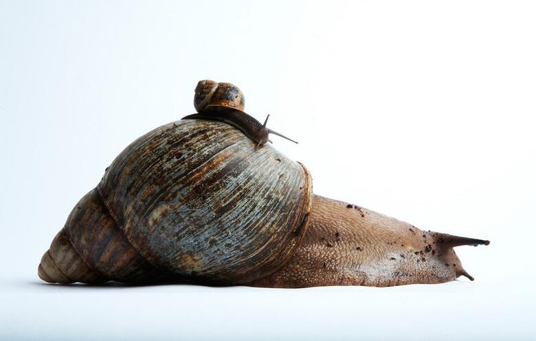
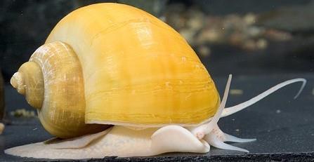
The Giant African snail (Lissachatina fulica) is an invasive snail that is native to East-Africa and is “one of the world’s most invasive pests.” (Dr Gabrielle Vivian-Smith, n.d) It is the world’s largest snail (see figure 1) with the largest measuring up to 39.3 centimetres (cm) in length and a shell length of 27.3cm.
(Guinness World Records, 2022) The Giant African Snail is a fast-reproducing snail and has a lifespan of up to 15 years. (Mongabay India, 2019) It is invasive to many different countries, including The United States of America, India, and the Solomon Islands.
Problem
The Giant African Snail invaded areas through trade routes, as they hitch hike on goods being imported to other countries. The main reason that the Giant African Snail is a problem is because it impacts heavily on the economy as it feeds on over 500 different species of plants, including coffee and pepper crops. (Mongabay India, 2019)
The Giant African snail can also carry a parasitic nematode that causes meningitis in humans. (University of Florida, 2011)
Solutions
There are not many solutions to exterminate this pest. Almost all solutions involve using pesticide or snail/slug pellets. The university of Florida presented a small-scale solution to be undertaken by US citizens, simply killings the snails with slug and snail pellets.
TheBestSolution
There are many different solutions, but one that has trailed and tested by the Central Coffee Research Institute in India has the largest impact. They devised an effective catch and kill method to wipe out the
10
Figure 1 (A common garden snail on top of the largest Land snail, the Giant African Snail. Guinness World Records, 2022)
pest. The created a bait made from rice bran, jaggery, castor oil and a chemical called Thiodicarb. They then placed this bait between crops to lure and kill the snails. The dead snails are collected, buried, and covered in salt to prevent the spread of diseases. In 2015 the Central Coffee Research Institute killed almost 30 tonnes of snails. (Mongabay India, 2019)
ReferenceList
Eastern Ecological Science Center 2018, Giant African Land Snail, United States government, USA, viewed 2 December 2022, <https://www.usgs.gov/centers/eesc/science/giant-african-landsnail#:~:text=Originally%20from%20East%20Africa%2C%20the,Basin%2C%20including%2 0the%20Hawaiian%20Islands.>.
Exotic invasive snails n.d., Australian Government, Department of Agriculture, Fisheries and Forestry, viewed 2 December 2022, <https://www.agriculture.gov.au/biosecurity-trade/pests-diseasesweeds/plant/giant-african-snail>.
Giant African Snail n.d., Critterfacts, viewed 12 December 2022, <https://critterfacts.com/giantafricansnail/>.
Largest land snail n.d., Guinness World Records, viewed 2 December 2022, <https://www.guinnessworldrecords.com/world-records/70397-largest-snail>.
Lissachatina fulica n.d., Wikipedia, viewed 2 December 2022, <https://en.wikipedia.org/wiki/Lissachatina_fulica#:~:text=Lissachatina%20fulica%20is%20a %20species,the%20Giant%20African%20land%20snail.>.
Mongabay India 2019, Battle against giant African snail invasion, online video, 1 August, viewed 8 December 2022, <https://www.youtube.com/watch?v=Hs5S6d5AyhI>.
University of Florida 2011, Giant African Snails, Florida, USA, viewed 12 December 2022, <https://sfyl.ifas.ufl.edu/archive/hot_topics/environment/giant_african_snail.shtml#:~:text=T o%20discourage%20these%20land%20snails,them%20a%20moist%2C%20sheltering%20env ironment.>.
11
Red Imported Fire Ants in Australia (Invasive)
Michael Mitchell (Year 7) The Illawarra Grammar School, 10/12 Western Avenue, Wollongong, NSW, Australia, 2500
The red imported ant species is a small ant that has a distinctive red colour Solenopsis invicta, originating in South America has soon invaded all over the world into major nations such as China, the USA and Australia (Factsheet 2017) and has been described as a super pest due to its severe damage cause and effect. it has been believed that fire ants have been accidentally imported worldwide from south America because of soil exporting. Fire ants were first discovered on February 11 2001 in Brisbane in a shipping container exported from America which had an outbreak of red imported ants decades ago in the 1940s in which the ants were seen as hitchhiking containers to and from containers this remained undetected due to biosecurity (according to Australian academy of science 2022) this caused a major biosecurity breach in which has made these red imported ant species an extreme pest
TheproblemsfireantscausetotheAustralianecosystem
Red fire ants have a devastating impact on Australia’s natural ecosystems as they can destroy natural seeds for vegetation that harvest honey drew which affects specialised invertebrates and makes them scavenge (Australian government of climate change, environment and water 2022). This in turn has the ability to destroy the entire Australian ecosystem as this can cause reducing plant populations as well as the creation of reduction of plant populations competing with native herbivores as well as insects in the search for food (Australian government climate change and environment water) Fire ants can not only cause devastating affects to Australian wildlife, however, can cause 3 billion dollars in damage to human-made objects to structural buildings, especially into circuit boards where short circuits for providing electricity to houses may be lost as a result, fire ants also chew on mechanical parts that can make them more prone to breakage as well as filling circuit boards full of soil to make their burrows calling it home. Lastly, fire ants can cause minor injuries to humans from their bits in which symptoms only consist of a small rash with swelling and pain around the side of the bit this generally last 3-8 days causing few to be alarmed (Fire Ants Information 2022).
Thepotentialsolutionsthatcanresolvesuchproblems
A range of solutions have been thought of when considering the prevention of problems fire ants cause which has been backed up with new technologies these include the tracking and location of fire ant nests in order for their nest to be destroyed and destroy the population in order to fewer numbers another thing that has been considered about the fewer population approach is to use dogs in order to sniff and locate the nest in which they can also destroy the nest of the ants causing a decrease in population, lastly another proposed plan in order to manage the pest population is to do aerial surveys from bird's eye view to track down nest and population, all these proposed plans have been thought under by the (Australian academy of science 2022) A couple of other effective plans have also been the use of locating ant trails and using sprays which will knock down population deeply decreasing the changes of Australia’s natural ecosystems to be extinct (pest control 2022) these measures have been seen as successful in providing this goal.
12
Whichsolutionisbestandwhy
The most effective way for the prevention of fire ants is to use baits and sprays used specifically on ants and their nest cin order to have accurate basis on the goal of eleminating such pest, the use of baits and sprays have proven to be of a success as it is currently the most effective treatment to stop the pest (pest control Australia 2022).
References
Arrow exterminators n.d., Red Imported Fire Ants, viewed 5 December 2022, <https://www.arrowexterminators.com/learning-center/pest-library/ants/red-imported-fireants>.
National diesease outbreak and pest 2021, Red Imported Fire Ants, viewed 5 December 2022, <https://www.outbreak.gov.au/current-responses-to-outbreaks/red-imported-fireant#:~:text=Red%20imported%20fire%20ant%20(RIFA,national%20cost%2Dshared%20erad ication%20programs.>.
Department of climate change and energy the environment and water 2021, Red imported fire antSolenopsis invicta, viewed 5 December 2022, <https://www.dcceew.gov.au/environment/invasive-species/insects-and-otherinvertebrates/tramp-ants/red-imported-
fire#:~:text=They%20destroy%20seeds%2C%20harvest%20honeydew,herbivores%20and%20i nsects%20for%20food.>.
Invasive species council 2017, Red fire ant, viewed 5 December 2022, <https://www.dcceew.gov.au/environment/invasive-species/insects-and-otherinvertebrates/tramp-ants/red-imported-
fire#:~:text=They%20destroy%20seeds%2C%20harvest%20honeydew,herbivores%20and%20i nsects%20for%20food.>.
Invasive species council n.d., How fire ants arrived in Australia, viewed 5 December 2022, <Invasive species council 2017, Red fire ant, viewed 5 December 2022, .>.
ABC news Australia 2015, How fire ants arrived in Australia, viewed 5 December 2022, <https://www.abc.net.au/news/2015-07-16/sniffer-dogs-help-fight-battle-against-fire-ants-inqueensland/6623876>.
Vansity termite and pest control 2021, The fire ant problem and how to fix it, viewed 5 December 2022, <https://varsitytermiteandpestcontrol.com/the-fire-ant-problem-and-how-to-solveit/#:~:text=Spray%20Ants%20and%20their%20Trails,back%20to%20their%20apparent%20s ource.>.
Australian academy of science, PG 2022, Fire ants: Australia's battle with red imported fire ants, 9 August, viewed 5 December 2022, <https://www.youtube.com/watch?v=-8d2wUx6jDo>.
National fire ant eradication program 2020, Treating fire ant nests, viewed 5 December 2022, <https://www.fireants.org.au/training-and-tools/tools-and-resources/farming/treating-fire-antnests>.
13
Lionfish (Pteroisvolitans)
The problem
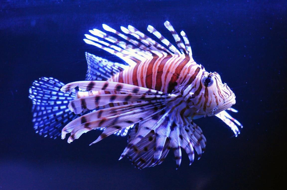
The lionfish (see figure 1) is an invasive species that has begun flourishing in the U.S. and Caribbean coastal waters. The species is not only invasive but has gone straight to the top of the food chain preying on native species and disrupting the natural ecosystem. The lionfish is native to Australia and the surrounding water, found in the South pacific and Indian oceans.
The lionfish is believed to have arrived on Florida’s coasts in mid 1890s when the first recorded sighting was made. Since its arrival in America’s coasts the lionfish population has grown dramatically, and lionfish now inhabit the many environments such as reefs or shipwrecks in the warm waters of the Atlantic. (NOAA Fisheries).
Though the lionfish is a unique and interesting spectacle this fish is not having a positive impact on all those who see it. Being an invasive species, the lionfish is disrupting many natural ecosystems and having a detrimental effect on other creatures. Because the lionfish has no natural predators except humans (most likely because of their venomous spines) the population is booming, throwing natural ecosystems out of order. The lionfish is eating many native fish and small animals unbalancing the natural food chains resulting in overpopulation for some species and underpopulation for others.
The potential solutions
Since lionfish have become such a problem there are now many strategies to control the population and save the natural ecosystems of our oceans. One of these strategies is hunting them, the most common way is spear fishing (see Figure 2) as it is very affective. Another strategy is a robotic zapper an idea that was introduced in 2015 by Colin Angle CEO for iRobot.
14
Edie Taggart (Year 7)
The Illawarra Grammar School, 10/12 Western Avenue, Wollongong, NSW, Australia, 2500
Figure 1: Lionfish ©Arc Net
The best solution
The best solution so far to the lionfish problem is spearfishing, hunting the fish by hand. This is because it is safe for other animals and is relatively easy to orchestrate. Though the problem of lionfish continues there is hope that this invasive species will return to its natural ecosystem.

Reference
Akpan, N & Ehrichs, M 2016, How do you stop invasive lionfish? Maybe with a robotic zapper, viewed 5 December 2022, <https://www.pbs.org/newshour/science/robot-lionfish-invasive-species-risenekton>.
NOAA Fisheries 2022, Impacts of invasive Lionfish, viewed 5 December 2022, <https://www.fisheries.noaa.gov/southeast/ecosystems/impacts-invasivelionfish#:~:text=The%20common%20name%20%E2%80%9Clionfish%E2%80%9D%20refe rs,in%20the%20past%2015%20years.>.
15
Figure 2: A speared lionfish ©Saltwater Experience
Giant African Snails
Jamie Vickery (Year 7)
The Illawarra Grammar School, 10/12 Western Avenue, Wollongong, NSW, Australia, 2500
TheProblem
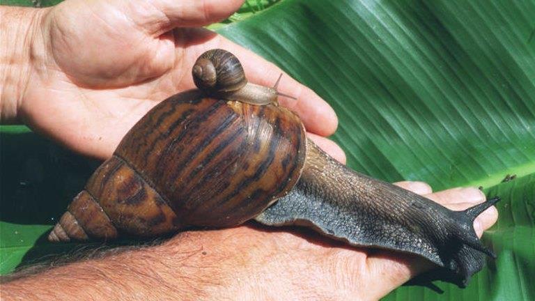
Giant African Snails have travelled the world becoming invasive by sneaking into imported food packages and being taken as exotic pets. These snails have originated in Eastern Africa. This snail has invaded many continents such as Asia and northern America. This big snail is 6 times the size of your regular garden snail. This snail eats over 500 different species of plants. Meaning it is a very serious threat to the agriculture of many countries. These snails can lay up to 1500 eggs in a year. The newborn snails will live underground for up to 6 months. In the US this snail has no natural predators meaning human control is the only option. This snail has the potential to destroy entire species of native plants due to its large appetite.
PotentialSolutionsandwhatoneisbest
The University of Florida states that it is using iron and sodium-based baits to kill of the Giant African Snails. Bait is the most effective way to kill these snails. A possible risk to this method is that other native animals may eats this bait resulting in them dying and the bait would have to be plated and dead snails collected daily. This is by far the most time effective method to reduce the population of Giant African Snails. Other methods include hand capturing and restricting their Snails area by creating fencing and restrictions. These methods simply take far more effort for worse results.
References:
HOW TO IDENTIFY AND CONTROL GIANT AFRICAN SNAILS 2021, viewed 2 December 2022, <https://www.corrys.com/resources/from-pet-to-threat-the-giant-africansnail#:~:text=The%20University%20of%20Florida%20advises,effective%20against%20Giant %20African%20Snails.&text=Iron%2Dphosphate%2Dpowered%20Corry's%20Slug,and%20k ill%20Giant%20African%20Snails.>.
Queensland Government 2019, Giant African snail, Queensland, viewed 8 December 2022, https://www.business.qld.gov.au/industries/farms-fishingforestry/agriculture/biosecurity/plants/priority-pest-disease/giant-african-snail
Department of Agriculture 2021, Exotic Invasive Snails, viewed 8 December 2022, <https://www.agriculture.gov.au/biosecurity-trade/pests-diseases-weeds/plant/giant-africansnail>.
16
Feral Pig
Luke Hughes (Year 7)
The Illawarra Grammar School, 10/12 Western Avenue, Wollongong, NSW, Australia, 2500
TheProblem
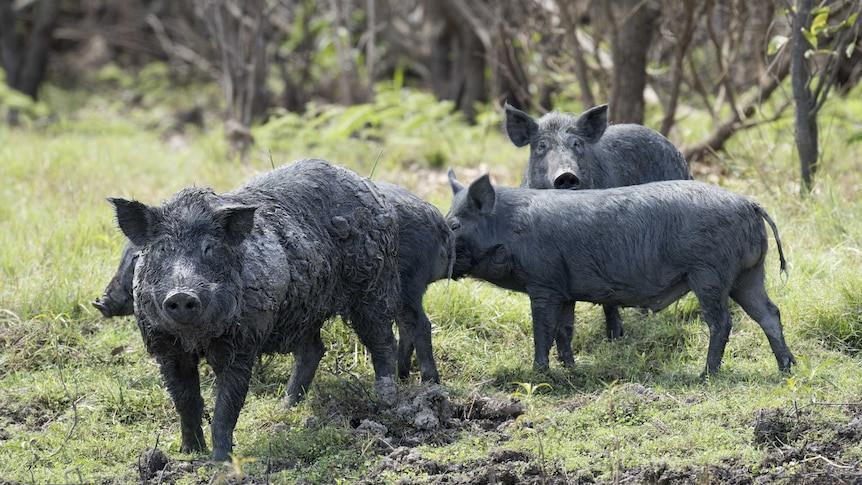
There is a huge problem with feral pigs in northern Queensland. Feral Pigs are Queensland's most widespread and damaging pest animal. Feral Pigs Spread invasive plants, dig up the soil, degrade the water, damage crops and livestock and carry disease. The Queensland Government state that you can’t move, feed, give away, sell or release feral pigs into the environment. About 40% of Feral Pigs in Australia inhabit sub plain grasslands to monsoonal floodplains.
TheSolution
Control methods include poisoning, trapping, exclusion fencing, ground shooting and shooting from helicopters. Commercial harvesters also use traps to capture pigs for export as wild boar meat. Prior to trapping, free feeding of bait is offered at sites where pigs are active. Trapping feral pigs can be effective in reducing numbers whereas, in areas where poisoning can’t be done safely, it's most successful when food resources are limited.
Whichsolutionisbest?
The best way to maintain the number of feral pigs is to place traps or hunt the feral pigs (Pestsmart N.D). Trapping the feral pigs or hunting them can rapidly reduce the number of feral in Northern Australia. Although this will not kill out the feral pigs because they are fast breeders, the feral pig spread across wide areas into thick bushland causing humans to not trap or kill as many.
References
Queensland Government 2022, Queensland Government, Queensland Government, viewed 8 December 2022, <https://www.business.qld.gov.au/industries/farms-fishing forestry/agriculture/biosecurity/animals/invasive/restricted/feral-pig>.
Pestsmart n.d., Pestsmart, viewed 8 December 2022, <https://pestsmart.org.au/toolkitresource/trapping-of-feral-pigs/#:~:text=Control%20methods%20incl ude%20poisoning%2C%20trapping,sites%20where%20pigs%20are%20active.>.
17
Golden Apple Snails
The Problem:
This species of Apple Snails are located in Vietnam, after being introduced from South America (Linh, 2021). The Golden Apple Snail was introduced for a few ideas. One of which was for food, as they can grow to 8 cm long, and can be consumed (Government of South Australia, 2020). They were also introduced with the idea for Aquarium trade, as they can grow quite large and become a pretty golden color, hence the name. However, the snail's introduction to Vietnam did not go as planned.
Shortly after being introduced, these slimy creatures quickly reproduced, spreading throughout Vietnam, settling into the many rice fields of the Vietnamese countryside. They are now classified in the Global Invasive Species Program as one of the top one hundred most invasive species (GISP, 2022). With a ranging diet of greens, these little pests have taken a liking to the rice crops around Vietnam, eating the base of the rice plants, destroying the whole plant (Knowledge Bank, 2022) These snails reproduce at rapid rates, laying up to 300 eggs at one time. They have now spread all over the many rice fields of Vietnam, and are extremely hard to exterminate due to the vast number of them and limited predators in their habitats.
Potential Solutions:
There are a range of different solutions which have been created to try to limit and kill off these snails (Knowledge Bank, 2022). One of which is the use of pesticides to try to poison the snails. These pesticides are usually applied to the areas of water in the fields where the snails live. However, these pesticides can sometimes affect the growth of the plants, and the empty packages are often left lying around the farms, littering the rice fields. Another solution is to place a barrier where the water (which the snails travel and live in) enters and exits the rice fields. This would also block other animals from traveling to and from the farm, however there are no necessary animals that have to travel to and from the fields, so this solution would not be a problem.
Best Solution:
I believe that the best solution to minimize the damaging effect of these golden critters is to place the barriers to block the water from entering and exiting the rice fields, as I talked about in the previous section. This should be done to keep all other snails from entering the fields, and then the use of pesticides could be used to eliminate all the snails left trapped in the field.
18
Leon Do (Year 7)
The Illawarra Grammar School, 10/12 Western Avenue, Wollongong, NSW, Australia, 2500
References:
Linh, P 2021, Invasive snails immune to pesticides in central Vietnam, viewed 4 December 2022, <https://e.vnexpress.net/news/news/invasive-snails-immune-to-pesticides-in-central-vietnam4222664.html#:~:text=Originating%20from%20South%20America%2C%20the,and%20veget able%20crops%2C%20among%20others.>
Plant Biosecurity, P 2017, Golden Apple Snail, viewed 1 December 2022, <https://www.dpi.nsw.gov.au/biosecurity/plant/insect-pests-and-plant-diseases/golden-applesnail#:~:text=Mature%20golden%20apple%20snails%20are,the%20mouth%20of%20the%20s hell.>
Golden Apple Snail n.d., viewed 4 December 2022, <http://www.knowledgebank.irri.org/step-by-stepproduction/growth/pests-and-diseases/golden-applesnails#:~:text=Golden%20apple%20snails%20eat%20young,base%2C%20destroying%20the %20whole%20plant.>
Biosecurity, S 2020, Golden Apple Snail, pdf, viewed 3 December 2022, <https://pir.sa.gov.au/__data/assets/pdf_file/0008/369791/Factsheet-Golden-Apple-snailAugust-2020.pdf>
Global Invasive Species Program 2022, viewed 2 December 2022, <https://www.gisp.org/>
19
The Burmese Python
 Zacariah Rusin (Year7)
The Illawarra Grammar School, 10/12 Western Avenue, Wollongong, NSW, Australia
TheProblem
Starting in the 1980s, the swamps of the South Florida have been overrun by one of the most damaging and invasive species the region has ever seen, the Burmese python. The Burmese Python is native to a vast amount of Asia stretching from northeast India to China. Burmese pythons were introduced to Florida in the 1970s and 1980s when thousands of the snakes were imported to be sold as exotic pets. Some owners who were unable to handle the giant snakes released them illegally into the wild. Pythons compete with native wildlife for food, which includes mammals, birds, and other reptiles.
PossibleSolutions
Over 400 responders trained by the Conservancy can safely and humanely capture and remove pythons or other exotic constrictors they encounter. Currently this solution has not had much effect on the population and trouble that the Burmese python are doing. Whichsolutionisbestandwhy?

Our innovative solution involves baiting the cages with pheromones, so that the snakes believe they are tracking the scent of the opposite sex. Since Burmese Pythons are usually solitary creatures. They believe this solution will work because it will attract many male pythons during breeding season and cut down the population growth.
Bibliography
The nature conservancy 2019, Python Patrol: Stopping a Burmese Python Invasion, viewed 2 December 2022, <https://www.nature.org/en-us/about-us/where-we-work/united-states/florida/stories-inflorida/stopping-a-burmese-python-invasion/>.

The Everglades Under Attack n.d., Solutions, viewed 2 December 2022, <http://pythonpatrol.weebly.com/>.
Georgiou, A 2022, How Burmese Pythons Invaded Florida with 100,000 Now Roaming the Everglades, viewed 2 December 2022, <https://www.newsweek.com/burmese-pythons-invaded-florida-100000roaming-everglades1720356#:~:text=Burmese%20pythons%2C%20which%20are%20one,them%20illegally%20i nto%20the%20wild.>.
Robins, R 2012, Burmese Python, viewed 2 December 2022, <https://www.floridamuseum.ufl.edu/100years/burmesepython/#:~:text=The%20Burmese%20Python%20is%20native,and%20is%20an%20excellent %20swimmer.>.
20
Lionfish

Baden Balding (Year 7)
The Illawarra Grammar School, 10/12 Western Avenue, Wollongong, NSW, Australia
Problem:
As the lionfish population rise there are even more problems that occur. An example of this includes destroying the coral. As the Lionfish has been introduced to areas in the Caribbean and Bermuda triangle. In these areas there are a sudden rise of population in the number of Lionfish. This causes a decrease in coral which causes native species to die. The main native animals and plants that were affected are Herbivores like zoo plankton, Primary Consumers and produces like coral. The lionfish don’t only eat creatures, but they get eaten. In America their main predators are Snapper, Grouper and other important native species. Since the Lionfish have poison when eaten the consumer most of the time dies. This could overpopulate or make animals or plant extinct which would interrupt the whole food chain.
Solution:
Lionfish are one of the many problems in the world that can never be fixed, but there are some ways that the American and Caribbean community are trying to fix this devastating problem. The first solution is Eat ‘em to Beat ‘em, as lionfish are a very tasty people like eating them. To convince people to catch them the let them keep them. The second competition is a fishing tournament when there is a prize or money people love to get involved. The last solution is spearing the fish, some people job in the world is to go around to kill lionfish. Since Lionfish are killing the coral reefs they need to control the population to take care of the native animals.
Bestsolution:
In my opinion the best solution is fishing tournament. In a tournament happens once a day with 50 boats with 6 people. And every day they catch 30 fish per 1 person with would equal 9000 fish per tournament which would significantly knock down the loin fish population. Plus, that’s just in one place out everywhere in the Caribbean and some America which could lead a lot of fish taken out of the ocean.
21
Foxy Loxy – The Red Fox
Zainab Zafar (Year 7)
The Illawarra Grammar School, 10/12 Western Avenue, Wollongong, NSW, Australia
TheProblem
The Red Fox is an invasive species in Australia. They were introduced into Southern Victoria in the mid-1800s. This was due to Victorian Settlers bringing them in, for hunting purposes. The red Fox originated during the Middle Villafranchian period in Eurasia. The Red Fox has caused the number of lambs, guinea pigs, rodents, rabbits and other native Australians to decrease. They have even caused the extinction of some species of bettong, the greater bilby, numbat, bridled nail-tail wallaby and the quokka. They heavily impacted farmers economically, as the Red Foxes preyed on farmers' lambs, poultry and kid goats. Overall, Red Foxes have caused a lot of damage for around 130 years.
Red Fox (Figure 1)

PotentialSolutions
There are currently many things being done to try and prevent significant damage from the Red Fox. This includes shooting, trapping, poison baiting, fumigation, animal husbandry, guarding animals, fertility control and fencing. However, all of these techniques fail to have a long-term effect. However, none of these methods on their own will prevent Red Foxes from causing damage.
Red Fox in a trap (Figure 2)

BestSolution
A skulk of shot Red Foxes (Figure 3)
Out of all these things being done to prevent the damage done by the Red Fox, the best solution would be fertility control. This is because unlike many of the other options, fertility control is a targeted method that will not harm other animals. Fertility control helps stop the population of Red Foxes to increase, as it stops female Red Foxes to give birth to offspring. Unlike this, options such as poison

22
baiting, fumigation, trapping and shooting can cause harm to other animals as well. Trapping and shooting can also be quite expensive. Furthermore, fencing is another option that is not the most suitable for this situation. This is because not only is fencing expensive, but it also does not decrease the population of Red Foxes, it just keeps them away from certain areas.
References
EUROPEAN RED FOX (VULPES VULPES) n.d., Australian Government, pdf, viewed 2 December 2022, <https://www.agriculture.gov.au/sites/default/files/documents/european-red-fox.pdf>.
Fox control n.d., viewed 2 December 2022, <https://www.dpi.nsw.gov.au/biosecurity/vertebratepests/pest-animals-in-nsw/foxes/foxcontrol#:~:text=Reducing%20the%20impact%20of%20the,effect%20on%20local%20fox%20 numbers>.

Johnson, C n.d., Is it too late to bring the red fox under control?, viewed 2 December 2022, <https://theconversation.com/is-it-too-late-to-bring-the-red-fox-under-control11299#:~:text=A%20brilliant%20piece%20of%20historical,occasions%2C%20beginning%20i n%20the%201840s>.
Red fox n.d., viewed 2 December 2022, <https://www.nwf.org/educational-resources/wildlifeguide/mammals/redfox#:~:text=Red%20foxes%20prefer%20rodents%20and,for%20being%20cunning%20and% 20smart.&text=Red%20foxes%20mate%20in%20winter>.
Red fox n.d., viewed 2 December 2022, <https://en.wikipedia.org/wiki/Red_foxhttps://en.wikipedia.org/wiki/Red_fox>. Red fox 2022, viewed 2 December 2022, <https://agriculture.vic.gov.au/biosecurity/pestanimals/priority-pest-animals/red-fox>.
23
Female Red Fox giving birth (Figure 4)
European Rabbits
Lulu Ding (Year 7)
TheProblem
The European rabbit, shown in figure 1, currently invades Australia in deserts and coastal plains, though they originally originated from Southwest Europe and Northwest Africa. In 1859, the European rabbits or ‘Oryctolagus cuniculus’ were first sent to Australia to Victoria, and received by a wealthy settler, Thomas Austin. It was sent to him by a relative who lived in Europe, and he let 13 of the rabbits run freely around his estate, which was located in Winchelsea, Barwon Park. These rabbits were also sent for hunting and game for people to shoot. Though, after around 50 years, these invasive species of rabbits had already spread around Australia, Coman (2022)

Furthermore, European rabbits have lead small ground mammals to extinction, Feral European rabbits (n.d.) and decreased the amount of native Australian plants and animals. Due to them overpopulating and enormous amount of plants they eat, other animals and bugs who needs those plants for survival, may also become extinct. The European rabbits also affect farmers, as they eat the crops meant for humans and grass for farm animals such as cows and sheeps. These types of rabbits also dig a lot, causing soil erosions, and making planting difficult.
ThePotentialSolutions
A potential solution to solve the overpopulation of the European rabbits is by poisoning them, or lethal baiting. Pindone is a popular poison for decreasing the European rabbits, as it reduces the ability for the blood clotting to happen inside the rabbits body. It is the most common poison to use, as it affects the rabbit the most, as when used on others animals such as dogs, they are 5-6 times more resistance than rabbits, rabbit control options (n.d.) and Pindone- A Poison For Rabbit Control (2022)
Another possible solution is to fumigate and destroy the Europeans warrens. People would spray toxic fumes into the warrens where European rabbits breed and live. By doing this, the rabbits will inhale the toxins, and become deceased shortly after, depending on the strength of the toxins, Sharp (2012).
24
The Illawarra Grammar School, 10/12 Western Avenue, Wollongong, NSW, Australia
Figure 1: European rabbits, Agriculture Victoria (2022).
Putting up fences is also a potential solution, and having it electric will improve the probability of it keeping out rabbits. This is because it divides the rabbits and the crops, as making it electric will shock the rabbits if it tries to go through it, Elsevier (1998).
Shooting and trapping rabbits is also a solution to decreasing the amount of European rabbits. It was written that, ‘ regular shooting can help maintain rabbit numbers at a low number, so that their impact is minimal,’ Dpi (n.d.).
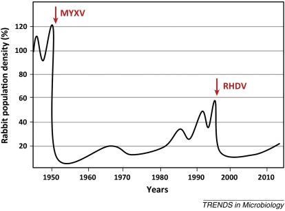
Thus, another possible solution is by spreading viruses that only affect rabbits. This can transmit through the infected rabbits urine, dropping, secretions and when they are mating. The myxoma virus and Rabbit Hemorrhagic desease Virus (RHDV), had already been spread. This can be avoided by other rabbits if they get vaccinated. Though, the rabbits became immune to the virus over time, RSPCA (2022).
Whichisthebestsolutionandwhy?
The best solution would be by introducing stronger viruses to wild European rabbits. This is because the past outburst of viruses given to rabbits in the 1950’s, called the Myxoma virus killed many invasive rabbits. This is shown in figure 2, as it displays the drop of the European rabbit population after the Myxoma virus was introduced. Likewise, in the 1980’s scientists introduced RHDV. This is spread by flies that carry around the desease called, ‘Ribonucleic acid,’ (RNA), and is a deadly virus that can kill infected rabbits within 48 hours. The decrease of the rabbit population can also be seen in figure 2, where the drop starts at the arrow painting downwards labeled, ‘RHDV,’ National Geographic (n.d.).
25
Figure 2: The European rabbit population from 1950-2010, Encyclopedia of Immunobiology (2016).
References:
Coman, B 2022, Rabbitsintroduced, viewed 4 December 2022, <https://www.dcceew.gov.au/sites/default/files/documents/rabbit.pdf>.
Department of Primary Industries n.d., Rabbitcontrol, viewed 4 December 2022, <https://www.dpi.nsw.gov.au/biosecurity/vertebrate-pests/pest-animals-in-nsw/rabbits/rabbitcontrol>.
Elsevier 1998, Long-termcosteffectivenessoffencestomanageEuropeanwildrabbits, viewed 4 December 2022, <https://www.sciencedirect.com/science/article/abs/pii/S0261219498000301>. FeralEuropeanRabbitn.d., Australian Government, pdf, viewed 4 December 2022, <https://www.dcceew.gov.au/sites/default/files/documents/rabbit.pdf>.
National Geographic n.d., HowEuropeanRabbitsTookoverAustralia, Washington, viewed 4 December 2022, <https://education.nationalgeographic.org/resource/how-european-rabbits-took-overaustralia>.
Pindone- APoisonforRabbitControl2022, Tasmanian Government, viewed 4 December 2022, <https://nre.tas.gov.au/invasive-species/invasive-animals/invasive-mammals/europeanrabbits/pindone>.
Rabbitcontroloptionsn.d., Bay Of Plenty Regional Council, pdf, viewed 4 December 2022, <https://www.boprc.govt.nz/media/395489/rabbit-control-options-a4-booklet-web-.pdf>
RSPCA 2022, WhatisrabbitcalicivirusandhowdoIprotectmyrabbitfromrabbithaemorrhagic disease?, viewed 4 December 2022, <https://kb.rspca.org.au/knowledge-base/what-is-rabbitcalicivirus-and-how-do-i-protect-my-rabbit-from-rabbit-haemorrhagic-disease/>.
Sharp, T 2022, Pestsmart, viewed 4 December 2022, <https://pestsmart.org.au/toolkitresource/diffusion-fumigation-of-rabbitwarrens/#:~:text=Other%20rabbit%20control%20methods%20include,rabbits%20leading%20to %20their%20death>.
Image References
Agriculture Victoria 2022, Europeanrabbit, Victoria, viewed 4 December 2022, <https://agriculture.vic.gov.au/biosecurity/pest-animals/priority-pest-animals/europeanrabbit>.
Encyclopedia of Immunobiology 2016, Myxomatosis, Science Direct, viewed 4 December 2022, <https://www.sciencedirect.com/topics/nursing-and-health-professions/myxomatosis>.
26
The Louisiana Crawfish
Maxwell Croft (Year 7)
The Illawarra Grammar School, 10/12 Western Avenue, Wollongong, NSW, Australia, 2500
The Louisiana Crawfish (Procambarus clarkii) is a subspecies of the red swamp crayfish. Like all of the other species of crayfish, this one is native to the Freshwater Rivers and other bodies of water in Northern Mexico, and the Southeast US.
Classification and Status
It’s various Binomial Nomenclature’s keys include: Malacostraca as the Class, Decapoda as its Order and Animalia as its Kingdom. It is not endangered, which is due to its vast majority of ever-growing population in the various states that it controls, like some parts of Canada and America.
The Problem
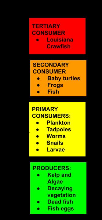
Its problem with the environment and economics is to do with their plantbased diet. They consume fish and some land mammals, but their main problem is the massive amount of algae, seaweed and various other vegetation, as shown in image 1. This makes dramatic shifts in the local food webs, and economically, decreases the value and numbers of fish in the market by eating their habitat and food sources / producers, thus making them less healthy.
A Potential Solution
A way to stop this Invasive Species is to use Bio-Accumulation. We put toxins into the producers of the food web, then the primary producers will eat the toxin in abundance and so on until the tertiary consumer, in this case the Crawfish. The Crawfish will die out or be controlled, and the toxin could be taken back somehow and let the fish population regrow without interference.
References
Wikipedia 2022, Procambarusclarkii, viewed 1 December 2022, <https://en.wikipedia.org/wiki/Procambarus_clarkii>.
National Park Services 2022, InvasiveCrayfish, viewed 1 December 2022, <https://www.nps.gov/articles/invasive-rusty-crayfish.htm>
27
The Small Indian Mongoose
Grace Lane (Year 7)
The Illawarra Grammar School, 10/12 Western Avenue, Wollongong, NSW, Australia, 2500
TheProblem
The small Indian mongoose was brought into many country’s including islands in the Caribbean, pacific and Indian oceans, as well as mainland south America and Europe to control pest rodents in sugar cane crops. It is native to parts of Iran, Asia, Malaysia, and Saudi Arabia. Indian mongooses have a big impact on the ecosystem, they eat every opportunity they get, but they mostly eat native birds, small mammals, reptiles, insect’s fruits, and plants, This can cause important animals in the food web to overpopulate and/or go extinct.
ThePotentialsolutions
Traps have become very popular to catch small Indian mongoose, Poison as bait is also an alternative to getting rid of small Indian mongooses. Traps keep small Indian mongooses from going freely in the wild and eating all the other animals. It keeps them under control and stops them from creating chaos in the affected areas. The second strategy for getting rid of small Indian mongooses is poison. Poison is also very commonly used to control the Indian mongooses. Poison kills the small Indian mongooses and stops them from eating all the native animals and plants to that country or area.
References
https://www.daf.qld.gov.au/__data/assets/pdf_file/0013/71140/IPA-Indian-Mongoose-RiskAssessment.pdf
https://dlnr.hawaii.gov/hisc/info/invasive-species-profiles/mongoose/

28
The Red Fox – An Invasive Species


 Jo Hernandez (Year 7)
The Illawarra Grammar School, 10/12 Western Avenue, Wollongong, NSW, Australia, 2500
INTRODUCTION
Red foxes are an introduced species to Australia. They originally came from European countries but were introduced to Australia in 1870. They were introduced for recreational hunting. Within 20 years they were considered pests and within 100 they have spread everywhere over Australia, except Tasmania. Today, there are reported cases of red foxes in Tasmania, but they are not yet confirmed. They are most commonly found in Victoria because Victoria's climate and terrain is their ideal living conditions. However, they can survive and thrive in urban areas, alpine
THE PROBLEM
coasts.
They are almost in the top of the food chain; their only predators are birds of prey and dogs while they are cubs. This makes the red fox thrive. They are a pest because they eat many native creatures, have contributed to the extinction of many small Australian creatures, threaten livestock (like sheep, cows, and chickens) and through the transmission of disease they are known to carry such as rabies, mange and distemper. All of these can be spread to other animals. Overall, the red fox is considered a threat to 14 species of bird, 48 different mammals and 2 amphibians. Foxes however, also eat berries and fruit. Red foxes have also contributed to the getting rid of some other invasive plant species, such as boxthorn, blackberries, and sweet briar.
THE SOLUTION
I believe the best way to get rid of red foxes is ground baiting. Ground baiting is when a meat bait with poison is put underground and covered with loose soil. This stops creatures who want meat from


29
heaths, rainforests, and
Figure 1-3: Red foxes happily living in many different places, from desert to snow, to your own backyard
Figure 4-6:- A red fox eating a bird, A red fox hunting an echidna, A red fox in a suburban area.
getting to it, unless they know how to dig well, like a fox. The poisons that are most used include sodium fluoroacetate (1080) and para-amino propiophenone (PAPP). Both of these can only be acquired through authorized people. The best time to put these baits out is spring, June and July, when food demand is the highest. They lure in foxes and then when they eat the bait it takes about 5 hours before they die. During these 5 hours, the fox will fall unconscious before it dies. The downside to this is that dogs and other wild animals can possibly get to the bait before foxes and immediate vet treatment will be required if this does happen.
REFERENCES
2021. “Foxes.” NSW Environment and Heritage. https://www.environment.nsw.gov.au/topics/animalsand-plants/pest-animals-and-weeds/pest-animals/foxes#:~:text=The%20red%20fox%20
“Red Fox.” 2017. Agriculture Victoria. https://agriculture.vic.gov.au/biosecurity/pest-animals/prioritypest-animals/red-fox.
“European Red Fox” Queensland Government https://www.daf.qld.gov.au/__data/assets/pdf_file/0019/73810/european-red-fox.pdf
“Ground Baiting of Foxes with Sodium Fluoroacetate” Pet Smart https://pestsmart.org.au/toolkitresource/ground-baiting-of-foxes-with-sodium-fluoroacetate/
30
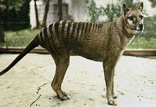
The Tasmanian Tiger - is it still alive?
Darby Parrish (Year 7)
The Illawarra Grammar School, 10/12 Western Avenue, Wollongong, NSW, Australia, 2500
The Tasmanian Tiger is a carnivorous wolf-like marsupial that was classified extinct in 1982. The Tasmanian Tiger or Thylacine lived throughout mainland Australia, Tasmania and New Guinea. These animals, although similar to the wolf in appearance, are marsupials and are an entirely different family to the placental mammals that wolves are. A Tasmanian Tiger looks like a wolf but does have some differences. The tail of a Tasmanian Tiger is stiffer, longer and has a smoother texture than the hairy tail of a wolf. The Tasmanian Tiger is covered in short shaggy fur, the body has a striped pattern across from its shoulders to feet. The head of a Tasmanian Tiger is fairly wide with small, rounded ears covered in short fur. The litter of a Thylacine was usually four and had a gestation period of up to 35 days. The offspring would stay with the mother till half grown. The pouch of a female Tasmanian Tiger was back opening and had four teats to provide a full litter with milk. The males also had a pouch, but it served as protective for their reproductive organs.
out at night mainly or sometimes during the day. The Tasmanian Tiger being a carnivorous animal would’ve adapted its waking times to suit when its prey was available. The Tasmanian tiger feasted on smaller animals like rats and other small mammals and its bone structure meant that it wasn’t adapted to taking on larger prey as before livestock was introduced the Tasmanian Tigers was one of the largest mammals in Australia. The Tasmanian Tiger would usually hunt in pairs walking with a stiff movement.
The Tasmanian Tiger died off due to illness, hunting and competition with introduced animals. When Australia was colonized, illness and non-native animals came with settlers. This ruined the existing ecosystem in Australia and greatly affected animals like the Tasmanian tigers. Not only being affected by illness and competition Tasmanian Tigers were hunted. Farmers saw they were catching animals and got scared that they would come after sheep and livestock so they killed them off. This led to the eventual extinction of the Tasmanian Tiger.
A rendered photo of the Tasmanian Tiger
The scientific name of a Tasmanian Tiger is Thylacinus cynocephalus which is translated to dog-headed pouched-dog. The Thylacine was a nocturnal or semi-nocturnal animal. Coming
The question is, is the Tasmanian Tiger still alive. While the Tasmanian Tiger was declared extinct many believe it is still alive. With many animals that are believed to be extinct being rediscovered many people have hope the Tasmanian Tiger will be next. There have been over 1000 reported sightings of the Tasmanian Tiger since it was classified extinct. A database was created with all these sightings and each sighting was given a rating of how reliable they were. While many sightings did prove to be unreliable quite a few stood out. People catching what looks like this mysterious wolf on camera and even scientists claiming they saw the Tasmanian Tiger. So is it still out there. Well it’s hard to tell. A study showed that there is a one in ten chance that the Tasmanian Tiger is still alive and others help reinforce the idea that it is still out there. But if the tiger is still alive why haven’t we found it yet and it was declared extinct.
31
Even if the Tasmanian Tiger is extinct, there’s still a possibility that the Thylacine may be alive once again. The University of Melbourne is trying to bring back the Thylacine through deextinction. This seems great to some but others are against it. They believe that if the Tasmanian Tiger went extinct then it should stay extinct. If we were to start bringing back animals from the dead where would it stop?
The Tasmanian Tiger was an incredible mammal unlike any other seen. Australia is so fascinated by it that it’s trying to bring it back from extinction or spot it once again. But is this the right thing to do or should the Thylacine remain extinct
32
How does light intensity affect photosynthesis?
Emmanuel O’Brien (Year 8)
The Illawarra Grammar School, 10/12 Western Avenue, Wollongong, NSW, Australia, 2500
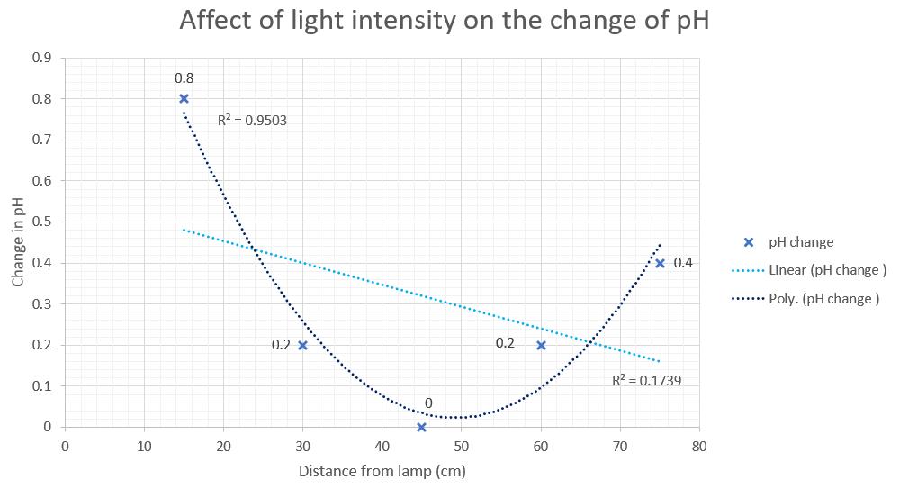
Results
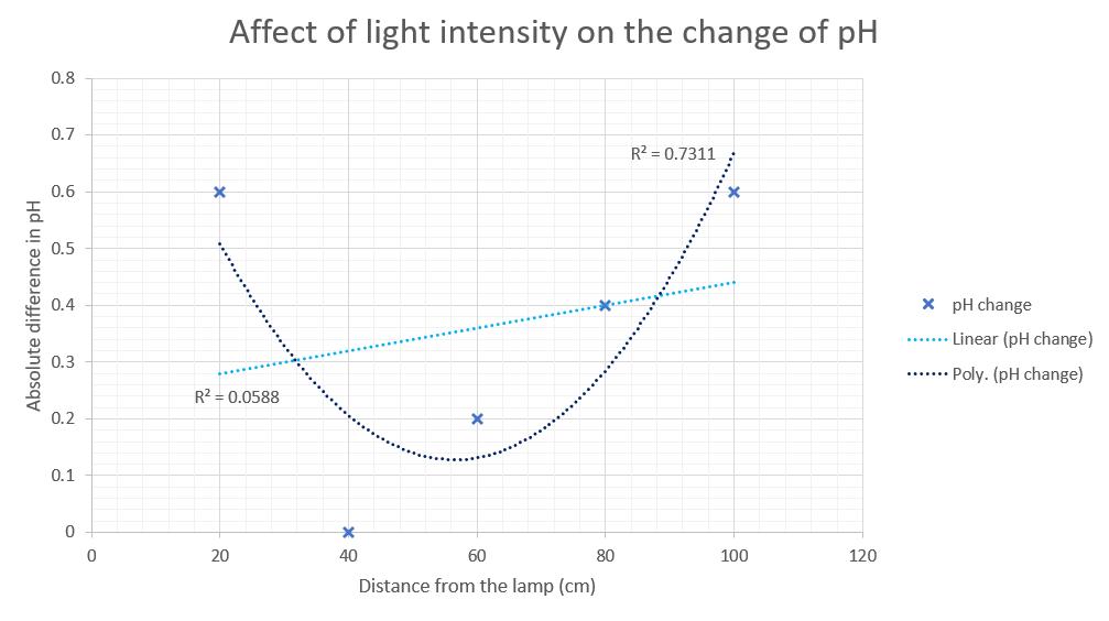
In the experiment conducted by class 8 O, both the closest flask of algae to the lamp and the furthest flask from the lamp had the greatest change in pH (Figure 1). Figure 2 shows the results from the experiment conducted by class 8 D. In both figures 1 and 2, there is a similar amount of change in pH in the flask closest to the lamp and the one furthest away. In both experiments the greatest changes occurred in the flasks that were closest to the lamp and furthest away from the lamp.
There are two lines of best fit shown in Figure 1 and Figure 2, a linear and a polynomial (nonlinear). Both figures 1 and 2 also show R² values. The R2 value is a measure of how well the line of best fit fits the data. R² values are marked from 0–1, 1 being the best fit for the data given in the graph. In figure 2, the linear line has an R² value of 0.1739 compared to the R² value of the nonlinear line which is 0.9503. This means that the non-linear line is by far the best fit for the data. In figures 1 and 2, there is a slight positive trend (Figure 1) and a slight negative trend (Figure 2) in the linear line of best fit, however because the R2 values are so low, these linear lines are unreliable and do not indicate a true positive or negative trend.
Discussion
This experiment aimed to determine whether light intensity affects the rate of photosynthesis. It was found that the more intense the light (closer to the lamp), the faster the rate of photosynthesis. Figure 1 and Figure 2 show that the algae closest to the lamp and the algae furthest away from the lamp had the greatest change in pH value. The non-linear trend line in figures 1 and 2 show this. The pH change closest to the lamp happened because the algae balls closest to the light had a high rate of photosynthesis where there was high light intensity, and the photosynthesis used carbon dioxide (took it out of the solution) which increased the pH value. The pH change furthest from the lamp happened because the algae balls were undergoing respiration at this furthest point, producing carbon dioxide and in doing so decreasing the pH value of the solution.
33
Figure 1: Results of experiment conducted by class 8 O (change in pH after 30 hours)
Figure 2: Results of experiment conducted by class 8 D (change in pH after 1.5 hours)
“Photosynthesis is the process by which plants use sunlight, water, and carbon dioxide to create oxygen and energy in the form of sugar” (Photosynthesis 2022). It is how most plants get their energy. They take light, water and carbon dioxide and create a sugar called glucose. Photosynthesis also produces oxygen, which is a by-product of this chemical reaction. Plants also respire. This is when they take in oxygen and use the glucose that they produced during the day and produce water (dew) and carbon dioxide. Photosynthesis happens in the light (mostly during the day) and respiration happens when there is less light (mostly during the night). A key difference between photosynthesis and respiration is the fact that photosynthesis produces energy while respiration consumes energy. Plants respire as this helps to keep the tissues in the plant healthy (M Gonzalez-meler, L Taneva, and R Trueman 2004)
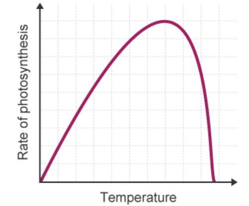
The results collected by class 8 O are reliable. When a similar experiment was undertaken by class 8 D the results had the same trend. Even though the graphs above (figures 1 and 2) have the same trendline, the two experiments had some important differences. The experiment conducted by class 8 O (Figure 1) left the algae balls out for 30 hours with 3 algae balls in each flask. The experiment conducted by class 8 D (Figure 2) left the algae balls out for 1.5 hours with 10 algae balls in each flask. These experiments were done under different conditions, yet both produced a similar result, indicating they are reliable. The results collected from the class 8 O experiment are valid. Variables like the number of algae balls in each flask were controlled, as was the amount of pH indicator (the liquid that the algae balls were in while the experiment was conducted) and the size of container that the algae balls were in. However, some variables were not controlled. These included temperature and other light sources in the room. These could affect the results. For example, as temperature increases, so does the rate of
photosynthesis (The effect of temperature on the rate of photosynthesis 2022). However, there is a point where the rate of photosynthesis starts to go back down. This starts to happen around 30℃. This occurs because the heat effects the function of the enzymes in the plants that carry out photosynthesis. As the temperature reaches around 40℃, then these enzymes can start to lose their shape, drastically decreasing the rate of photosynthesis (S Markings 2018) as seen in Figure 3.
This investigation is not as accurate as it could be. This is because the pH values collected were measured using a colour chart. The flasks were compared to this chart at the start and the end of the experiment to collect the pH values. As different people see colours differently, they may have recorded a different pH value even if the pH in the solution was actually the same. This could lead to inaccuracy, making it hard to compare results with others.
There are some improvements that could be made to this investigation. One main issue is that reading the exact pH is hard by just looking at it. If an electronic pH probe was used, then the results would be more accurate. Another way
34
Figure 3: This graph shows how temperature effects photosynthesis (Factors affecting photosynthesis 2022)
that this experiment could be improved is by controlling the environment more. This could be done by only having one light (so that other light in the room does not interfere with the experiment) and controlling the temperature (as that could also have affected the rate of photosynthesis).
This investigation aimed to determine if light intensity affects the rate of photosynthesis. It was hypothesised that as the plant received less light, the rate of photosynthesis would slow down. Once the data was collected and plotted in a graph it was found that the algae balls furthest from the light started to respire, meaning that instead of consuming carbon dioxide from their surrounding environment, they produced it and consumed oxygen. This made the graph have neither a positive or negative trend but have one that starts high, drops, and then rises again (see figure 1 and 2). One main limitation of this experiment is the measuring of the pH. This could be improved from comparing the colours of the flasks to a colour graph, to using an electronic pH probe to make the results more accurate. In the end, this experiment was valid and reliable enough to show that the intensity of light on plants effects their rate of photosynthesis and respiration, supporting the hypothesis.
References
Photosynthesis 2022, National Geographic, viewed 15 November 2022, https://education.nationalgeographic.
org/resource/photosynthesis
Gonzalez-Meler, M, Taneva, L & Trueman, R 2004, Plant Respiration and Elevated Atmospheric CO2 Concentration: Cellular Responses and Global
Significance, National Library of Medicine, viewed 10 November 2022, https://www.ncbi.nlm.nih.gov/pmc/ar
ticles/PMC4242210/
Markings, S 2018, The Effect of Temperature on the Rate of Photosynthesis, viewed 16 November 2022, https://sciencing.com/effecttemperature-rate-photosynthesis19595.html
Factors affecting photosynthesis 2022, BBC, viewed 16 November 2022, https://www.bbc.co.uk/bitesize/guides /zx8vw6f/revision/2#:~:text=As%20wi th%20any%20other%20enzyme,high% 20temperatures%2C%20enzymes%20a re%20denatured%20.
35
The relationship between light intensity and rate of photosynthesis

Rhys Chieng (Year 8)
The Illawarra Grammar School, 10/12 Western Avenue, Wollongong, NSW, Australia, 2500
Discussion
Extrapolated from the investigation, which aimed to determine the effect of light intensity on the rate of photosynthesis, found that as exposure to light increased, a large pH change in the algal balls was experienced. Similarly, as light exposure decreased, pH change also increased. A plot of two variables between the distance from the lamp and the change in pH showed a clear non-linear relationship. From the graph, a large pH change was measured when the algal balls were 20 cm and 100 cm away from the lamp whilst pH changes were unnoticeable around the 60-80 cm mark. The line of best fit showed a polynomial trend, which further showed that large pH changes were experienced when the algal balls were placed close and far away from the lamp.
The results clearly support the initial hypothesis of the experiment. This was strengthened by the fact that levels of pH correlate to the amount of carbon dioxide, thus linking to the rates of photosynthesis and respiration (2022, Britannica). Figure 2 below summarises the correlation between photosynthesis and cellular respiration. In photosynthesis, the reactants, carbon dioxide and water are added to form products, oxygen, and glucose. Photosynthesis is most active in the daytime, due to sunlight being the main catalyst for the reaction. Collision theory states that chemical reactions can be sped up by increasing the temperature (2012, TedEd). Since light produces heat, the higher the light intensity, the higher the rate at which photosynthesis occurs. In contrast, respiration uses oxygen and glucose to form water and carbon dioxide. Respiration is an ongoing
reaction and is most prominent at night, due to a lack of sunlight, thus causing photosynthesis to cease (2022, ProMix). These processes are essential for facilitating the growth of plants as well as maintaining a balance of oxygen and carbon dioxide (2021, Photosynthesis Education). Additionally, it is also very important to understand that these reactions are nearly opposite biochemical processes. Thus, the intensity of light a plant receives impacts the rate at which photosynthesis and respiration occur.
The results found in the investigation are considered unreliable as when comparing results with secondary sources, large differences between data collected were identified (E.g Mrs. Baird’s results showed a fluctuating trend where pH changes peaked at 60cm and 80cm). Although, Mrs Baird’s experiment was very different in the method, meaning that a direct comparison might not be accurate. Additionally, the experiment was not repeated, leaving potential for random error. However, no significant outliers were apparent.
In order to ensure validity, appropriate variables were measured and controlled. The dependent variable, pH change was measured in knowledge that pH corresponds to levels of carbon dioxide, thus linking to the rate of photosynthesis.
36
Figure 2: Photosynthesis, denoted as carbon dioxide + water → oxygen + glucose is most
Although variables such as the size of the algal balls and external light sources were not controlled, the intended aim was measured and answered, which facilitated a better understanding of how light intensity affects the rate of photosynthesis.
As a colour pH indicator was used to measure the change in pH, there could have been a potential that the results gathered were not precise and accurate due to the subjectiveness of colour scales. Thus, the determination of colour could have been executed better due to multiple students interpreting the pH of the vials differently. This was a human error that should be minimised in future experiments where qualitative and quantitative observations are crucial when tabulating results. However, when looking at figure 1, the absolute error was found to be 0.0106, thus showing that the results gathered were quite accurate. The small errors in accuracy were possibly a result of the pH indicator’s lack of objectiveness and precision.
There was room for improvement and potential to extend the investigation. Specifically, setting the experiment in a completely dark room with no external light would allow for an accurate measurement of the rate of photosynthesis. In the investigation, multiple experiments were conducted at once, thus resulting in many lamps to be active in the same room. Having multiple light sources going at once could have led to potential light pollution, thus affecting the accuracy of the measurements. Furthermore, the use of a pH probe would have led to more precise and accurate results due to its objectiveness. As mentioned previously, colour pH indicators are very subjective due to its use of colour determination for pH. The size and number of algal balls placed in each jar was also not consistent due to human error. This could be standardised by measuring the mass of each vial in which a consistent amount of algae could be placed in each vial.
This investigation could be extended further by assessing how light intensity affects the rate of photosynthesis in plants. Unlike algae, photosynthetic efficiency is not as efficient in plants (2022, Frontiers). Plants unlike algae have a vascular system, roots, and leaves (2020, Save Barnegat Bay). It would be interesting to compare how light intensity affects the rate of photosynthesis in plants and algae.
References
Britannica 2022, photosynthesis: Additional Information, viewed 9 November 2022, <https://www.britannica.com/science/ photosynthesis/additionalinfo#history>.
Frontiers 2022, Algal Photosynthesis, viewed 12 November 2022, <https://www.frontiersin.org/researchtopics/25172/algalphotosynthesis#:~:text=place%20on% 20Earth.,Photosynthetic%20efficiency%20is%2 0higher%20in%20algae%20than%20i n%20higher%20plants,5bisphosphate%20carboxylase%2Foxyge nase>.
Live Science 2021, What are Algae, viewed 12 November 2022, <https://www.livescience.com/54979what-are-algae.html>.
Photosynthesis Education 2022, Photosynthesis and Respiration viewed 9 November 2022, <https://photosynthesiseducation.com /photosynthesis-and-cellularrespiration/>.
Pro Mix 2022, Basics of Plant Respiration, viewed 9 November 2022, <https://www.pthorticulture.com/en/t raining-center/basics-of-plantrespiration/>.
Save Barnegat Bay 2020, What’s This Green Stuff? A Breakdown of Plants vs. Algae in
37
Barnegat Bay, viewed 12 November 2022, <https://www.savebarnegatbay.org/wh ats-this-green-stuff-a-breakdown-ofplants-vs-algae-in-barnegat-bay/>.
Science and Plants for Schools 2022, Measuring the Rate of Photosynthesis, viewed 8 November 2022, <https://www.saps.org.uk/teachingresources/resources/157/measuringthe-rate-of-photosynthesis/>
Science Sparks 2019, What is Respiration?, viewed 8 November 2022, <https://www.sciencesparks.com/what-is-respiration/>.
Ted-Ed, T 2012, How to speed up chemical reactions (and get a date) - Aaron Sams, online video, 19 June, viewed 7 November 2022, <How to speed up chemical reactions (and get a date)Aaron Sams>
38
The pH level of water after being exposed to carbon dioxide
Marci Davis-Cook (Year 9)
The Illawarra Grammar School, 10/12 Western Avenue, Wollongong, NSW, Australia, 2500
Introduction
Humanity’s dependence on natural resources to produce energy, and especially the methods used, are becoming detrimental to the environment. Not only does the burning of fossil fuels cause the depletion of non-renewable resources, but it also produces large amounts of carbon dioxide which when located in the atmosphere reflect heat towards the earth contributing to global warming (Fecht, 2021). As CO2 levels increase in the atmosphere, so too do the levels in the ocean, as proven in ‘Henry’s Law’ which states that the amount of carbon dioxide dissolved in a liquid will attempt to be equal with the amount of carbon dioxide in the air above (Orenda Technologies, n.d.).
Therefore, natural carbon sinks which remove excess CO2 produced by human activities, including the ocean which covers more than 70% of the Earth’s surface home to approximately 50-80% of all living-things (Marine Bio, n.d.), are absorbing more carbon dioxide than ever before - around a quarter of carbon dioxide found in the atmosphere is dissolved into the ocean with 22 million tons absorbed per day (Smithsonian, 2018). Moreover, in the past 200 years, after the Industrial Revolution, ocean water has become 30% more acidic becoming the fastest change in the past 50 million years (Smithsonian, 2018) with research suggesting that the increase of carbon dioxide levels is responsible for the alteration in the seawater’s pH levels, known as ocean acidification.
Ocean acidification is extremely threatening due to the abundance of marine life living in the ocean, the dependence on the ocean as a food
source, the ocean’s role in the water cycle and in regulating the Earth’s climate, ecosystems and more. For instance, ocean species that require shell protection, such as coral, are struggling due to the limited supply of carbonate ions which are depended on for production, since excess hydrogen ions created from carbon dioxide reacting with water are bonding with carbonate ions leaving little availability for shell production (NOAA, n.d.), and in some cases acidic waters are dissolving the shells. Furthermore, marine life is already suffering due to limited time to adapt to the new acidic conditions, which poses a risk towards the food chain (NOAA, n.d.) Moreover, the ocean plays a major role in the water cycle, being one of the main sources for evaporation to occur, and as a result of ocean acidification, precipitation can become acidic damaging the lithosphere, plants etc. In summary, the ocean is of vital importance and rising acidity levels are already proving to be threatening.
Therefore, this experiment aims to determine if the decrease in the pH levels of water is due to carbon dioxide.
Aim
To determine the effect of carbon dioxide (CO2) on the pH level of water (H2O).
Hypothesis
If carbon dioxide is combined with water, then the pH level of the water will decrease to become more acidic. This is because, when carbon dioxide reacts with oxygen, carbonic acid is formed which “dissociates” into hydrogen ions (H+) and carbonate ions (CO3 –2) which can be seen in the following equations:
(Atlas Scientific, 2021). Moreover, the pH scale measures the amount of hydrogen ions in a solution and the more of these ions means a substance is more acidic with a lower pH.
39
CO2 + H2O → H2CO3 H2CO3 → 2H+ + CO3 –2
Therefore, when carbon dioxide is added to water and hydrogen ions are released from the carbonic acid, the water’s pH level will decrease since the amount of hydrogen ions has increased (Smithsonian, 2018).
Method
To determine the effect of carbon dioxide (CO2) on the pH level of water (H2O), an experiment was conducted that mixed water with carbon dioxide produced from the acid-base neutralisation concept as seen in the following formula:
acid + base ⟶ water + salt + carbon dioxide (Jacaranda, 2018)
This experiment used the following chemical formula:
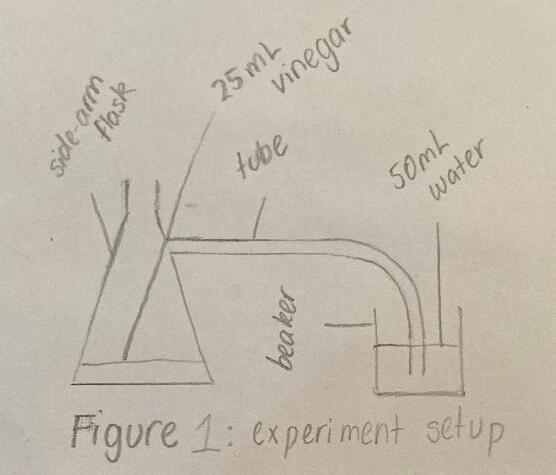
which was connected to a beaker filled with 50mL of water via a tube, as per Figure 1.
The amount of bicarb soda (independent variable) was changed so that the pH level of water (dependent variable) could be measured at different carbon dioxide amounts, therefore the trend could be revealed. This experiment was controlled by keeping the amount of vinegar (25mL) and water (50mL) the same to control the environment the reactions were performed in; the water source (taps in the science classrooms at TIGS) and the equipment (sidearm flask, balloon, tube, beaker etc) constant to control the chemical properties of the water and the environment the experiment was conducted in; emptying and refilling the vinegar and water after every test since otherwise the solution would already be neutralised and adding more bicarb soda would have no effect; and by waiting until all the fizzing of the vinegar had seized before measuring the pH of the water to ensure the product of carbon dioxide had been fully released.
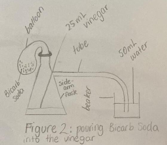
For this experiment, 25mL of vinegar was measured and poured inside a side-arm flask
To begin the first test, 1g of bicarb soda was placed into a beaker with a spoon and weighed accordingly using scientific scales and then poured into a balloon. After this, the balloon was carefully pulled over the lid of the side-arm flask, as seen in Figure 2, before the bicarb soda in the balloon was emptied into the vinegar causing a neutralisation reaction to occur as seen through the fizzing.
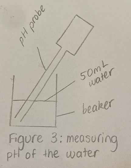
After the fizzing had seized, the tube was removed from the beaker and a pH probe was placed in the water, as shown in Figure 3. An app called ‘Vernier Graphical Analysis’ was downloaded and used to read the pH level displayed by the pH probe. Once the calculation was complete, the pH level of the water was recorded in a table and the pH probe was returned to its storage solution. To ensure the validity of this experiment, the beaker and side-
40
CH₃COOH + NaHCO₃ ⟶ H2O + NaCl + CO2
arm flask were cleaned and filled with new water/vinegar after every test, and the same steps were completed for bicarb soda amounts of 2g, 3g and 4g. Finally, to guarantee the reliability, this experiment was repeated and conducted 3 times.
Results
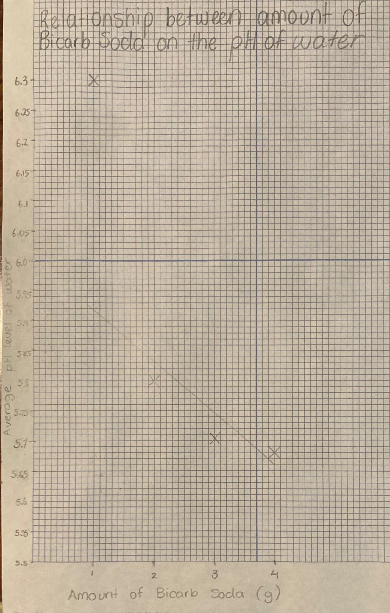
Table 1: The effect of carbon dioxide on the pH levels of water
41
Amount of bicarb soda (g) pH level Test 1 Test 2 Test 3 Avg. 1 6.4 6.2 6.3 6.3 2 5.7 6.09 5.61 5.8 3 5.7 5.6 5.84 5.713 4 5.81 5.61 5.62 5.68
42 Graph
Results
This graph shows that as the amount of bicarb soda increased (producing more carbon dioxide), the average pH level of the water decreased becoming more acidic. For instance, the average pH level of the water decreased to 6.3 when 1g of bicarb soda was used, and the average pH level became 5.68 when 4g was used. In summary, a definite decrease in the pH level of the water can be seen as carbon dioxide is added.
Discussion
As the amount of bicarb soda increased, and therefore the amount of carbon dioxide due to more reactants producing more products, the pH level of the water decreased becoming more acidic. Reasons for this are because when carbon dioxide and water react, dissolving the carbon dioxide, carbonic acid is produced which releases hydrogen ions amongst others responsible for the acidity of substances (Atlas Scientific, 2021). Therefore, the results from this experiment supported the hypothesis that water becomes more acidic when mixed with carbon dioxide and these results represent the effects of carbon dioxide on the ocean which is home to hundreds of thousands of marine species, depended on by humans as a food source, recreational place, and regulator of the Earth’s climate. These results prove that carbon dioxide is contributing to ocean acidification, which is damaging marine life, corroding soils, and overall impacting negatively on the environment. Even though the pH of water will not become acidic (drop below a pH of 7), the smallest changes have vast impacts as seen by the drop from 8.2 to 8.1 since the Industrial Revolution which has already seen the destruction of coral reefs and more (Smithsonian, 2018). For this reason, the results from this experiment are of extreme importance to proving that carbon dioxide is an issue altering the chemistry of seawater which means strategies need to be made that promote the reduction of greenhouse gas emissions.
This experiment can be considered fairly reliable since it was repeated three times and a clear trend can be seen from calculating the averages showing a definite decrease in the pH level of water after carbon dioxide was added. However, some of the results were inconsistent, for example, in ‘Test 3’, 2g of bicarb soda made the pH level 5.61, whereas 3g made the pH 5.84. These results do not coincide with the trend that more bicarb soda, and as a result more carbon dioxide, decreases the pH level of the water, which is due to the solution becoming saturated and the vinegar being a limiting reagent. For instance, in the first test of 1g, the bicarb soda acted as the limiting reagent since it was determining the quantity of carbon dioxide being produced. On the other hand, as the amount of bicarb soda increased to 4g, the vinegar (25mL) limited the amount of carbon dioxide being produced as there were no atoms left to react with the extra amounts of bicarb soda, which made the vinegar the limiting reagent (Blanchard, 2016). If this experiment was to be conducted again, then more vinegar would be included improving this experiment’s method and therefore its validity, but also improving the consistency of the results and as a result, its reliability.
Furthermore, the method used to conduct this experiment allowed the relationship between the pH level of water and the amount of bicarb soda, ultimately the amount of carbon dioxide, to be determined and so can be considered a valid test. Further improvements of validity could be seen through better controlling some of the control variables, including the time at which the water’s pH level was measured. Instead of relying on human observations to decide when the fizzing of the vinegar and bicarb soda solution had seized, leaving the results at risk of human error, a timer could have been set to measure all tests at a precise moment. This would have made sure that the measuring of pH occurred at a consistent point in the stages of the
43
chemical reaction taking place improving the validity of this experiment. Moreover, for the test to be more valid in terms of its abilities to represent ocean acidification, the use of seawater instead of tap water would have allowed the test to be a closer sample with properties more like the ocean. Another aspect of this investigation that could use improvement is the method at which the bicarb soda was poured into the side-arm flask. By pouring the contents from the balloon, some bicarb soda ended up being left inside, and although this may have minimal impact, it does change the amount of bicarb soda being tested. New methods at inserting the bicarb soda to ensure all remnants had been added would be beneficial to the validity of this experiment.
Finally, the use of a pH probe instead of other methods like pH indicators, allowed this investigation to record more accurate measurements. However, the figures took a while to calibrate as the measurements appeared to ‘jump around’ before finally settling. Nevertheless, the findings of this experiment are accurate due to the use of modern equipment.
Conclusion
An experiment was conducted to determine the effect of carbon dioxide on the pH level of water. The hypothesis that the pH level of the water would decrease (becoming more acidic) as carbon dioxide was added, was supported. It was found that as the amount of bicarb soda being poured into the vinegar to produce carbon dioxide increased, the pH level of the water decreased. However, some of the results were inconsistent as the vinegar/bicarb soda solution became saturated due to the vinegar becoming a limiting reagent when the amount of bicarb soda increased, meaning that the maximum amount of carbon dioxide had been produced with left over solute unused slowing the decrease of the water’s pH. Yet a clear trend showing the effect of carbon dioxide on the pH of water was still determined from calculating the averages. In
summary, the findings in this investigation are extremely relevant as the continued release of greenhouse gas emissions from human activities, like the burning of fossil fuels for energy, are detrimental not only to the atmosphere, but also the hydrosphere and in turn all four of the Earth’s spheres. If more can be understood about the effects of greenhouse gas emissions, like the effect of carbon dioxide on the ocean, then promotions for change and strategies to combat the climate crisis can occur.
References
Blanchard, J 2016, Limiting Reactant and the Baking Soda/Vinegar Reaction, online video, 18 February, viewed 23 October 2022,
<https://www.youtube.com/watch?v=8 gAmC2fED6o>
Fecht, S 2021, How Exactly Does Carbon Dioxide Cause Global Warming?, Columbia Climate School, viewed 24 October 2022,
<https://news.climate.columbia.edu/2 021/02/25/carbon-dioxide-causeglobal-warming/>
How Does CO2 Affect PH In Water? 2021, Atlas Scientific, viewed 24 October 2022, <https://atlas-scientific.com/blog/howdoes-co2-affect-ph-in-water/>
Jacaranda 2018, Neutralisation, viewed 18 October 2022, <https://content.jacplus.com.au/faces /pages/ebookviewer.xhtml?isbn=07303 54067&pk=3589e213c5f86f8e&cb=90 64763443604941786>
Lindsey, R 2022, Climate Change: Atmospheric Carbon Dioxide, NOAA, viewed 24 October 2022,
<https://www.climate.gov/newsfeatures/understandingclimate/climate-change-atmosphericcarbondioxide#:~:text=Without%20carbon% 20dioxide%2C%20Earth's%20natural,
44
causing%20global%20temperature%20 to%20rise.>
Marine Life n.d., Marine Bio, viewed 23 October 2022,
<https://www.marinebio.org/creatures /facts/#:~:text=An%20estimated%205 0%2D80%25%20of,living%20space% 20on%20the%20planet.>
Ocean Acidification n.d., National Oceanic and Atmospheric Administration, viewed 24 October 2022,
<https://www.noaa.gov/education/res ource-collections/ocean-coasts/oceanacidification>
Orenda Technologies n.d., CO2 and pH: Understanding Henry's Law, viewed 25 October 2022,
<https://blog.orendatech.com/co2and-ph-henrys-
law#:~:text=The%20pH%20ceiling&te xt=That%20point%20of%20equilibriu m%20is,this%20ceiling%2C%20but% 20not%20naturally.>
Smithsonian 2018, Ocean Acidification, viewed 22 October 2022,
<https://ocean.si.edu/oceanlife/invertebrates/ocean-acidification>
45
Ocean acidity and its impacts
Alexis Evans (Year 9)
The Illawarra Grammar School, 10/12 Western Avenue, Wollongong, NSW, Australia, 2500
Introduction
The economies of many countries around the world are dependent upon the ocean, but it and all the organisms that reside in it are slowly being damaged by ocean acidification. Ocean acidification is “the reduction of pH of the ocean over an extended period of time, caused primarily by uptake of carbon dioxide (CO2) from the atmosphere” (NOAA n.d.). The pH scale is a measure of how acidic or basic a substance is, ranging from 14, meaning very basic, to 1, which is very acidic. A pH of 7 means that a substance is neutral, such as pure water. Seawater, with all of its additives, has a basic pH. Since the industrial age, carbon dioxide levels in the atmosphere have been rising due to the burning of fossil fuels for energy and land use change. The ocean absorbs approximately 30% of the carbon dioxide that is released into the atmosphere (NOAA n.d.). Though the effects of this carbon dioxide absorption are not outwardly noticeable, it can cause great damage beneath the surface (Smithsonian Ocean 2018).
When carbon dioxide is absorbed into water, a chemical reaction occurs which produces carbonic acid, which lowers the pH of the water to become more acidic. The ocean is very vast, and would require a great deal of carbon dioxide to change the pH of such a large expanse of water, but it is predicted that approximately 525 billion tons of carbon dioxide has been absorbed into the ocean since the industrial era, changing the ocean’s chemical make-up to become 30% more acidic (Smithsonian Ocean 2018). Because the change in pH has been so rapid, the fastest change in ocean chemistry in 50 million years, marine life that exists within the Earth’s oceans has not been given the time to adapt and protect itself from the changing environment. Some
creatures’ shells dissolve in more acidic seawater, and corals are also more difficult to build and maintain in such a foreign environment (NOAA n.d.).
The chemistry behind the process of ocean acidification is quite simple; deceptively so for how much destruction it causes. When carbon dioxide enters the seawater and reacts with it to produce carbonic acid, the pH of the ocean is lowered. The creation of this acid binds carbonate ions, making less available for the corals, oysters, mussels and other sea creatures that need them to build shells and skeletons (Smithsonian Ocean 2018). Carbonic acid is a relatively weak acid, so can not actually change the entire ocean acidic, but it does make it lean dramatically towards being acidic. The ocean pH has dropped so far from 8.2 to 8.1 since the industrial revolution, when large amounts of carbon dioxide began to be emitted into the atmosphere, and is predicted to drop another 0.3 to 0.4 pH units by the end of the century (Smithsonian Ocean 2018).
This experiment aims to simulate the chemical reaction between water and carbon dioxide in ocean acidification and investigate the effect of the amount of sodium hydrogen carbonate as the base in a neutralisation reaction on the pH of water after carbon dioxide is produced and bubbled into the water to form carbonic acid. Because carbon dioxide is a gas and would be difficult to capture to use for the experiment, a neutralisation reaction will first be completed to the necessary carbon dioxide for the ocean acidification simulation reaction. A neutralisation reaction occurs between an acid and a base and makes the resulting solution one with a neutral pH of 7. However, for the resulting solution to be fully neutral, the acid and base must fully cancel each other out, which means they must be in equal amounts. The reactants that will be used in this investigation are acetic acid, commonly known as vinegar, and
46
sodium hydrogen carbonate. This reaction can be represented by the chemical equation:
CH3COOH + NaHCO3 → H2O + CO2 + NaC2H3O2 (vinegar + sodium hydrogen carbonate → water + carbon dioxide + sodium acetate).
The products of a neutralisation reaction are always water and a salt. In the case of the base in the reaction being a carbonate, such as sodium hydrogen carbonate, the reaction will also result in carbon dioxide. When this neutralisation reaction is completed, the carbon dioxide it produced will be transferred into a volume of water and the pH will be measured after the acidification reaction has taken place. Since the equipment needed to measure how much carbon dioxide is used in the secondary reaction is not available, the data collected will be of how much sodium hydrogen carbonate is added to the vinegar, since that amount will be proportional to the amount of carbon dioxide produced and transferred into the second reaction. The chemical equation for the main reaction of this investigation is:
H2O + CO2 → H2CO3 (water + carbon dioxide → carbonic acid).
It is hypothesised that the outcome of this investigation will be that the carbon dioxide will make the water more acidic and lower the pH to below 7, in the acidic range. This is because when carbon dioxide meets water and reacts with it, it forms carbonic acid. Since water has a neutral pH neutral, the solution of the carbonic acid and water will then become more acidic with a lower pH. This means that the more sodium hydrogen carbonate is added to the vinegar in the neutralisation reaction, the more carbon dioxide will be produced and then transferred into the secondary reaction, and therefore more carbonic acid will be produced. Ultimately, the more sodium hydrogen carbonate is added to the neutralisation
reaction, the lower and more acidic the pH will be from the water acidification reaction. If the impacts, causes and severity of ocean acidification can be understood, it can be properly addressed before it becomes an overly major issue, and all the economies in the world that rely upon fishing and the ocean to survive will prosper once again.
Methodology
Independent variable: The independent variable in this investigation is the amount of sodium hydrogen carbonate (commonly known as bicarb soda) added to the vinegar to react to form carbon dioxide.
Dependent variable:
The dependent variable in this investigation is the pH of the water and carbonic acid solution after the reaction between the sodium hydrogen carbonate and vinegar. The pH will be measured using a fully-charged pH probe inserted into the solution, and the results will be read in an exact number on the application that connects the probe to an electronic device.
Controlled variables:
There are several factors in this experiment that must be controlled. The amount of vinegar used in the chemical reaction to create carbon dioxide must be regulated across all tests to ensure that the amount of carbon dioxide can be proportional across all tests. If the amount of vinegar changes and the amount of sodium hydrogen carbonate changes, then it would be impossible to know how much carbon dioxide was entering the beaker of water. In that case, then the results of the experiment would be meaningless because the investigation would not be valid. This variable can easily be controlled, by simply deciding upon an amount to use for every test and measuring out that amount using an electric scale. The amount of vinegar that will be used is 80mL. The amount of water in the beaker must also be controlled throughout the investigation, because the pH would vary depending upon the concentration of the acid. The concentration of the acid would vary in
47
different amounts of water, affecting the validity of the results.
The amount of water in the beaker can be controlled in the same way as the amount of vinegar in the flask. For each repetition of the experiment, the same amount of water can be measured out into the beaker using the electric scale. 120mL of water will be used. The pH of the water the carbon dioxide will be bubbled into must also be controlled. It would be difficult to change the pH to make it exactly the same for each repetition without modifying the outcome of the experiment, but if the water is sourced from the same location it is most likely to have the same pH. The initial pH of the water will be measured using a pH probe, and if there is a larger difference than 0.5 between the pH, that water will not be used.
The water will be sourced from the same tap, so that should ensure the pH will be maintained across the investigation. To make sure that the measuring of the pH of the water is accurate every time, it must be ensured that when the sodium hydrogen carbonate reacts with the vinegar, the solution does not bubble up enough to reach the level of the side-arm in the flask and enter the beaker of water and carbon dioxide. If either of these reactants enter the water and carbon dioxide solution, they would affect the validity of the results, because the sodium hydrogen carbonate is a base and would increase the pH, while the vinegar is an acid and would decrease the pH. Any additive would therefore alter the pH that was given by the experiment, and render the results invalid. Finally, the method of measuring the pH in this investigation must be maintained so that the results can all be recorded in the same way. If universal indicator were used for one test, then a pH probe used for another, the results would not be comparable and would thus be meaningless. The method of pH measurement used in this investigation will be a pH probe.
Equipment list:
• 1 Side-arm flask
• 1 Funnel
• Vinegar
• 100mL beaker
• 150mL beaker
• 200mL beaker
• 1 Balloon
• Sodium hydrogen carbonate
• 1 pH probe
• 1 Electric scale
• 1 spoon
• Water
• Rubber tub
Method
1. The rubber tube was attached to the arm of the side-arm flask, and the flask was filled with 80mL of vinegar, which was measured into the 150mL beaker on the electric scale before it was poured into the flask.
2. For the first test, 3g of sodium hydrogen carbonate was measured into the 100mL beaker on the electric scale using the spoon. The sodium hydrogen carbonate was then poured, with the use of the funnel, into the balloon.
3. The opening of the balloon was stretched over the top opening of the side-arm flask so that the seal was airtight. It was done carefully to prevent any of the sodium hydrogen carbonate from being tipped into the flask prematurely.
4. The 200mL beaker was filled with 120mL of water from the tap, again using the electric scale. The pH probe was set up and inserted into the water. After the pH reading settled and had stopped changing to reach a definitive number, the pH probe was removed from the water.
5. The end of the rubber tube not attached to the side-arm flask was inserted into the water in the beaker and the opening was fully submerged.
48
This set up can be seen the diagram below.
6. While the rubber tubing was held in place in the beaker, the balloon attached to the top of the side-arm flask was inverted and the sodium hydrogen carbonate it contained was emptied into the vinegar within the flask. As the chemical reaction occurred between the sodium hydrogen carbonate and vinegar, the rubber tubing was held in place to ensure all carbon dioxide created from the primary reaction was captured to create the secondary chemical reaction with the water.
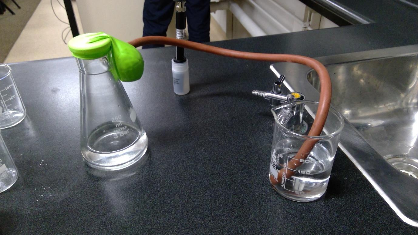
7. After the primary chemical reaction between the sodium hydrogen carbonate and vinegar had subdued and no more bubbles of carbon dioxide gas was being released into the water, the rubber tube was removed from the water and carbonic acid solution and the pH probe was once again inserted. The pH was measured.
8. The flask, rubber tubing, pH probe and beakers were rinsed out with water, and then the same process was repeated twice more with the amounts of sodium hydrogen carbonate of 5g and 7g.
49
Results Water pH Amount of sodium hydrogen carbonate (g) Initial Post-reactive 3 6.87 5.89 5 6.82 5.25 7 6.93 7.16
Diagram: Set up of the equipment in preparation for the experiment
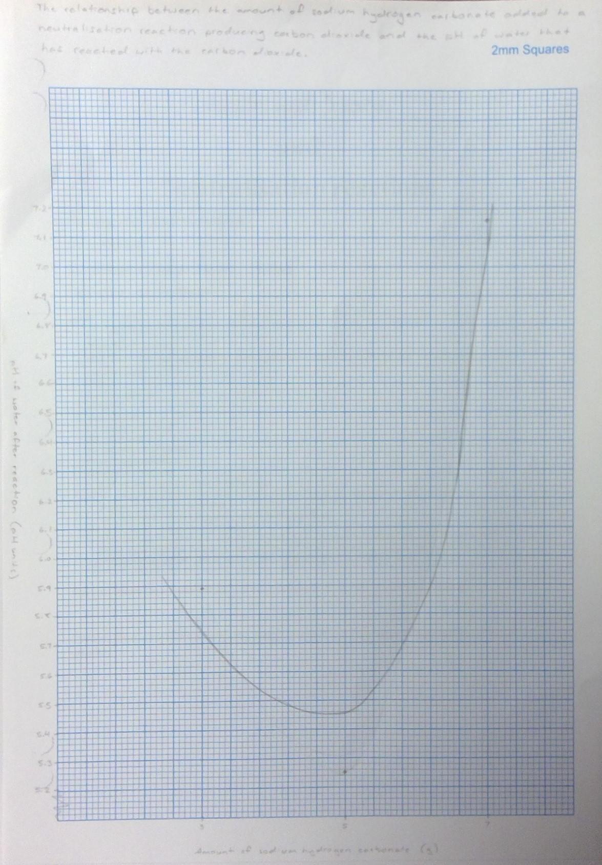
50
The graph is non-linear and does not show a relationship between the two variables. At first, when the independent variable increased, the dependent variable decreased, showing a negative relationship. Then, however, the dependent variable increased when the independent variable increased.
Discussion
The were no visible trends or relationships present in the results, and the aim of the investigation was not achieved. The aim was to investigate the effect of the amount of sodium hydrogen carbonate as the base in a neutralisation reaction on the pH of water after carbon dioxide is produced and bubbled into the water to form carbonic acid. The test using 7g of sodium hydrogen carbonate has an apparently outlying result, but this cannot be confirmed because the results were not reliable as they were not repeated at all. The hypothesis for this experiment was not supported by the gathered results, which was that as the amount of sodium hydrogen carbonate increased, the pH of the water would decrease to become more acidic. This was refuted because, while the first two results supported this, the last result did not.
The results of the experiment were not accurate, valid or reliable. There were several issues with how the investigation was carried out, the most important one being that there were no repetitions of the tests of each amount of sodium hydrogen carbonate. If each amount had been trialled at least three times, any outliers in the data could have been easily identified. The average could also have been found to have a more accurate representation of what the results were like. In addition, the accuracy was very low mostly in the third amount tested. Because so much vinegar was used in the neutralisation experiment, when 7g of sodium hydrogen carbonate was added, the chemical reaction bubbled up the neck of the flask and spilled out the rubber tubing into the beaker of water and carbon dioxide. This was a failure to control all
the necessary variables, and greatly affected the validity of the result. Since the vinegar was still mostly at the bottom of the flask, the majority of the solution that entered the water beaker was sodium hydrogen carbonate, the base from the neutralisation reaction. Because it had a higher pH, it changed the results to be higher than they would have been had there been no sodium hydrogen carbonate in the beaker. Since bases have a higher pH, there was so much sodium hydrogen carbonate that it overpowered the amount of carbon dioxide to change the pH of the water to become higher and more acidic rather than lower and more basic.
The results, had the experiment been completed correctly, would have supported the hypothesis and shown that as the independent variable increased, the dependent variable decreased as the water and carbon dioxide solution became more acidic the more carbon dioxide was added. This is because whenever carbon dioxide molecules meet water molecules, a chemical reaction occur, which always produces carbonic acid, without exception. Since water is neutral with a pH of 7, the carbonic acid would lower the pH and turn the solution acidic. If this is not the case, then another factor would be interfering with the results such as in this investigation.
To improve the method, each change of the independent variable should be tested at least three times to improve the accuracy and reliability of the results and to remove any risk of unidentified outliers skewing the results away from what they should have been. Also, if less vinegar was poured into the flask for the neutralisation reaction, there would be much less risk of the solution bubbling up to interfere with the second reaction. This would make the results more valid because the base used in the neutralisation reaction would not be changing and influencing the measured pH of the water and carbon dioxide solution.
51
Conclusion
The aim of this investigation was to determine the effect of the amount of sodium hydrogen carbonate as the base in a neutralisation reaction on the pH of water after carbon dioxide is produced and bubbled into the water to form carbonic acid, and it was hypothesised that as the amount of sodium hydrogen carbonate was increased, the pH level of the water would decrease. The results showed no clear relationships between the two factors, therefore refuting the hypothesis, because in the first two tests, the pH did decrease, but in the final test it increased as the amount of sodium hydrogen carbonate did also. However, only one repetition was done of each change of the independent variable, so the experiment could not be considered reliable. Also, in the third test an amount of the products and reactants from the neutralisation reaction unintentionally entered the beaker of water and carbon dioxide, thereby making the results invalid and inaccurate. Even so, the findings of this investigation can contribute to helping understand the impact and issue of ocean acidification, and can provide a basis for a solution to be found to the threat it poses to the world’s oceans.
References
National Oceanic and Atmospheric Administration (NOAA) n.d., What is Ocean Acidification?, viewed 27 October 2022, <https://oceanservice.noaa.gov/facts/a cidification.html>.
Smithsonian Ocean 2018, Ocean Acidification, viewed 27 October 2022, <https://ocean.si.edu/oceanlife/invertebrates/ocean-acidification>.
52
Ocean Acidification and Carbon Dioxide
Samuel Robinson (Year 9)
The Illawarra Grammar School, 10/12 Western Avenue, Wollongong, NSW, Australia, 2500
Introduction
The aim of this experiment is to determine and investigate the effect of carbon dioxide (CO2) on the acidity levels of dihydrogen monoxide (water/H2O), when sodium hydrogen carbonate (NaHCO3) reacts with vinegar (acetic acid) to produce carbon dioxide (CO2).
This aims to prove the effect ocean acidification which occurs because of carbon dioxide released by greenhouse gases. “Carbon dioxide (CO2) is a colourless, odourless and non-poisonous gas formed by combustion of carbon and in the respiration of living organisms and is considered a greenhouse gas (group of gases contributing to global warming)” (Glossary: Carbon dioxide emissions 2017, Eurostat, <https://ec.europa.eu/eurostat/statisticsexplained/index.php
title=Glossary:Carbon_dioxide_emissions#:~:te xt=Carbon%20dioxide%20emissions%20or%2 0CO,as%20well%20as%20gas%20flaring>).
Carbon dioxide (CO2) emissions stem from the manufacturing of cement and the burning of fossil fuels such as coal that help to provide electricity. As of 2021 around 36.4 billion metric tonnes of carbon dioxide are produced annually. "Some 30 percent of all CO2 dissolves into seawater, where it doesn't remain as floating CO2 molecules. A series of chemical changes break down the CO2 molecules and recombine them with others.” (Bennett, J 2018, <https://ocean.si.edu/oceanlife/invertebrates/ocean-acidification>). When CO2 dissolves into sea water it mixes to produce carbonic acid (H2CO3) which is a weaker acid comparatively. Even though carbonic acid is weaker and acts slower it still produces hydrogen
ions (H+) like other acids. The concentration of these released hydrogen ions (H+) are often referred to acidity and the more hydrogen ions an aqueous solution contains the more acidic the substance is. The increase of these hydrogen ions (H+) or increase in acidity in sea water is called ocean acidification and the result of ocean acidification is the reduction of the amount of carbonate in the ocean. Carbonate is a key building block in sea water life and the reduction of carbonate results in making it more difficult for marine life such as plankton or coral to form their shells and skeletons and possibly even dissolve them. This results in changes in growth, development and abundance as the lack of a fully formed shell results in marine life becoming more vulnerable throughout their life especially in their juvenile stages.
Therefore, it can be hypothesised that when the amount of sodium hydrogen carbonate is increased by (2,8,16 grams) more carbon dioxide will be produced and the ph levels of the water will decrease and become more acidic. This is because when vinegar reacts with sodium hydrogen carbonate (NaHCO3) the chemicals neutralise and from carbon dioxide in the form of gas bubbles. The carbon dioxide will dissolve into the water and react forming carbonic acid which releases hydrogen ions (H+). Hydrogen ions when combined with water molecules will increase the acidity level as hydrogen ions are directly linked to acidity levels.
Variables Independent
Increasing the amount of sodium hydrogen carbonate (NaHCO3) by (2.1, 8.1, 16.1 grams) in order to increase the amount of carbon dioxide, which was measured by using an electronic scale. This is important to the experiment as changing the amount of NaHCO3 increases the amount of neutralisation between the acetic acid (vinegar) and sodium hydrogen carbonate (NaHCO3)
53
which produces more carbon dioxide which is part of the aim of the experiment.
Dependant
The pH levels of the water after the carbon dioxide gas bubbles produced in the sidearm eventually disappeared, which was measured by pouring 15 droplets of universal indicator into the water (H2O) prior to each trial run and the colour after the trial was matched against the universal indicator chart. This is important because measuring the pH levels is what will determine if the water became more acidic or not after carbon dioxide was produced.
Controlled
Amount of acetic acid (vinegar) - This is important because if the amount of vinegar increases the amount of neutralisation occurring will slightly decrease which will produce less carbon dioxide during each trial changing the acidity of the water in each trial. This was measured by using a separate 100mL beaker to measure out 75mL of acetic acid each trial before pouring the acetic acid into the sidearm flask.
Leftover biproducts and water from trials in the 500mL beaker and sidearm flask – Cleaning out the 500mL beaker and sidearm flask was done after each trial to clean out the acidic water from the 500 mL beaker to prevent the water in the following trials from becoming more acidic affecting the reliability of the experiment. The sidearm flask was cleaned out to remove the left over biproducts of the acetic acid and NaHCO3 reaction which would have reacted with the acetic acid poured in the following trial which would have created carbon dioxide to early and would have left through the top of the beaker with no balloon.
Amount of universal indicator drops – This is important because changing the amount of universal indicator droplets in the water in each
trial changes how clear or unclear the pH level appears by making the pH level appear more or less in each trial affecting the accuracy of the experiment. This was controlled by pouring exactly 15 droplets of universal indicator with each droplet being poured slower so it could be counted.
Amount of water – The amount of water is important because changing the amount of water in each trial means more or less carbon dioxide is needed to increase the pH levels so the pH levels will vary more drastically in each trial if the amount of water is more or less in each trial. This was measured by using a 500mL measuring beaker to consistently measure 100mL of water during each trial.
Equipment List
• 1x Sidearm Flask
• 2x Beakers
• 1x Silicon Tube
• 2x 100mL Beakers
• 1x 500mL Beaker
• 1x Universal Indicator
• 1x Tripod
• 1x Electronic Scale (Including Power Cable in Plastic Bag)
• 1x Vinegar Glass
• 1x Indicator Scale Chart
• 1x Spoon
• 1x Cone Funnel
• Sodium Hydrogen Carbonate
Container
Method
1. The silicon tube was attached to the arm of the sidearm flask
2. The electronic scale plug was removed from the plastic zip lock bag and plugged into the power point on the side of the desk
54
3. The electronic scale was then plugged in and the power point was turned on
4. One of the 100mL beakers was placed on the electronic scale and the scale was set to zero, using a spoon 2.1 grams of sodium hydrogen carbonate (NaCOH3) was scooped from the NaCOH3 container and poured into the 100mL beaker
5. The NaCOH3 mass was weighed to make sure it was 2.1 grams (this was done to keep the NaHCO3 close to 2, 8 and 16 grams after being poured through the funnel as it was expected that some amount would be lost in the funnel reducing it below 2 grams), before 100mL of water (H2O) was poured into the 500 mL beaker from the tap
6. 50 mL of acetic acid (vinegar) was then poured from the glass into the remaining 100 mL beaker to make sure it was 50 mL, before being poured into the sidearm flask with the arm side facing away to prevent the acetic acid falling through the tube
7. The rubber balloon was then attached to the smaller end of the cone funnel before the NaCOH3 was then poured from the 100mL beaker into the larger end of the funnel and into the balloon
8. The open end of the balloon was then attached around the top of the sidearm flask with caution to prevent the NaHCO3 from falling into the sidearm flask and beginning the reaction prematurely
9. Using the universal indicator fifteen droplets were poured into the beaker containing water (H2O) and the colouration was measured the universal indicator chart to make sure the colour matched pH level 7
10. The metal sheath was then placed onto the tripod before the sidearm flask was placed on the sheath with at least one
hand holding the sidearm flask while it was on the tripod
11. The unattached end of the tube was placed inside the 500 mL beaker before the balloon was flipped vertically, pouring the NaHCO3 into the sidearm flask and beginning the reaction
12. The reaction was then observed with the 500mL beaker being closely observed for colour change in the water until the carbon dioxide gas bubbles within the sidearm flask disappeared
13. The colouration of water in the 500 mL beaker was then matched against the universal indicator chart and the pH level matching the water’s colouration was then recorded
14. The balloon was removed from the sidearm flask and both the sidearm flask and 500 mL beaker were washed out in the sink using tap water, with the arm side of the flask pointing away from the sink to prevent the acetic acid and NaHCO going into the tube when washed out with water to prevent either product falling into the 500 mL beaker containing water in the next trial altering the trial to make the water more of a base or acid
15. Steps 4 to 14 were then repeated another two times using 2.1 grams of NaHCO3
16. Steps 4 to 15 were then repeated two times using 8.1 grams and then 16.1 grams of NaHCO3
55
Results
Figure 3. A graph including a trendline showing the decrease in pH water levels as the
NaHCO3 amounts increase with each increase being labelled as a dot
As seen in both Figure 2 and 3 the relationship between carbon dioxide and water pH levels is found to be a linear relationship with the water pH levels always decreasing and becoming more acidic as the carbon dioxide levels increased from increased amounts of NaHCO3. It can also be observed that this was a steady increase as on the right of Figure 2. it can be seen that the average dropped by 0.1 each time and not by varying amounts. Finally, a slight decrease by 0.5 in 1 out of the 3 trials of each increased amount can be seen in the pH levels which has led to the
averages dropping by 0.16 and becoming a decimal.
Discussion
The results found in Figure 2. and 3. supported the hypothesis that as the amount of sodium hydrogen carbonate (NaHCO3) increased the amount of carbon dioxide will also increase, decreasing the waters pH levels making it more acidic. This is seen most clearly in Figure 3. as the graphs trendline shows that the pH levels decrease at a steady rate, as the amount of NaHCO3 increased. This highlights that the relationship between carbon dioxide and water pH levels is linear as when one goes up the other goes down. This linear relationship can also be seen in the Figure 2. table as the averages on the right decrease by 1.0 each time the amount of NaHCO3 increases on the right, again showing a clear linear relationship with no sudden increases in water pH levels. Therefore, it can be observed that water pH levels will always steadily decrease into becoming more acidic if more carbon dioxide is added to water. However, the results in Figure 2. do show that 1 out 3 trial attempts decrease by a further 0.5 in pH levels which could highlight that more carbon dioxide was absorbed by the water, which still proves a linear relationship supporting the hypothesis but does question the accuracy slightly. These results though are also supported by scientific evidence as carbon dioxide (CO2) dissolved in water (H2O) will combine and produce carbonic acid (H2CO3), which is a weaker type of acid. “The weaker carbonic acid may not act as quickly, but it works the same way as all acids: it releases hydrogen ions (H+), which bond with other molecules in the area” (Bennett, J 2018, <https://ocean.si.edu/oceanlife/invertebrates/ocean-acidification>).
Because the concentration of hydrogen ions is what determines acidity of an aqueous solution the water becomes more acidic as more hydrogen ions bond with water molecules. This can be seen in the results as the increased
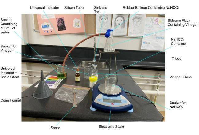
56
Figure 1. A diagram of the experiment conducted during a trial, including all the listed materials
amount of NaHCO3 (on the left of the table and bottom of the graph) leads to increased amounts of carbon dioxide due to neutralisation with the acetic acid which mixes more carbon dioxide with water to create more carbonic acid. And because carbonic acid releases hydrogen ions more carbonic means that more hydrogen ions are produced increasing the concentration of the hydrogen ions making the water more acidic, decreasing the pH levels as seen on the right of table.
The experiment was highly valid as all the necessary conditions were met throughout the experiment with the controlled variables all being met with the correct response. With the acetic acid and water amounts being correctly measured within separate measuring beakers and most importantly the 500mL beaker and sidearm flask being cleaned out after each trial run was conducted to remove left over biproducts. The results found also correctly matched the scientific evidence with the pH levels of the water decreasing as the amount of NaHCO3 and acetic acid produced carbon dioxide increases due to the creation of acidic carbonic acid. This means that the results found are backed up and supported by scientific evidence and have clear valid reasoning on why it appears as such. Additionally, efforts to reduce the loss of NaHCO3 grams when poured through the cone funnel were also made as it would make the amount of NaHCO3 actually reacting with acetic acid less than aimed for and therefore somewhat invalid. Thus 0.1 grams of NaHCO3 were added each trial to make up for the loss and get closer to the exact gram amount, however, 0.1 grams was made as a estimated guess for the loss and not an accurate amount so instead a better method of getting the NaHCO3 into the balloon needed to be found perhaps by pouring it directly into the balloon carefully.
The experiment was mostly accurate as during the experiment universal indicator was used to measure the pH levels, also a scale was used to
measure the amount of NaHCO3 in grams, while measuring beakers were used for both water and acetic acid (vinegar amounts). The use of the scale in measuring the amount of NaHCO3 was highly accurate as the scale rounded to at least 1 decimal place making it more accurate to measure close to 2, 8 and 16 grams as it could be observed if the amount was slight over or below, however, further accuracy could have been achieved if the scale had been able to round to further decimal places but the achievability of matching to more decimal places when scooping would have been harder. The use of measuring beakers for both the water and acetic amounts was also highly accurate in making sure the water was at 100mL and the acetic acid was at 75mL as it prevented the need to guess amounts which may have caused varying amounts instead of similar amounts for each trial. The use of the universal indicator was only mostly accurate however, as even though the same number of droplets were poured in each time and a chart was used to measure the colouring of the water, the results were based slightly off judgement on whether the colour was closer to one acidity level or another which did create slight variations in results that may have affected reliability. This could have been improved upon by using a pH probe instead which would have provided a more accurate quantitative judgement based off the hydrogen ions in the instead of the colouration of the water.
The reliability of the experiment was shown to be mostly high as each of the increased amounts of NaHCO3 were repeated 3 times over to generate an average. This was done to show if the water pH levels of the first trial was actually reliable or whether a mistake had been made that produced the wrong pH level making the extra two trials important in proving whether the results were reliable by seeing if the results were close together in pH levels. Each of the pH levels in the 3 trials were close together with only 1 out
57
of 3 trials for each increase of NaHCO3 producing a different pH level which was only 0.5 pH levels below the other two trials. Additionally, the reliability of the results is best shown in the averages which are 0.16 below 2 out of the 3 trials making it highly reliable as the difference is very. Whilst the difference does not look like a massive difference in the results making the experiment seem highly reliable a “pH scale is logarithmic (pH = -log[H+]), a change of one pH unit corresponds to a ten-fold change in hydrogen ion concentration” (PMEL, <https://www.pmel.noaa.gov/co2/story/A+pri mer+on+pH>). Meaning that there is a somewhat significant difference in the results as a slight change by 1pH level is a large increase or decrease, however the results only differ by 0.5 and 0.16 which isn’t a massive damage to the reliability of the experiment. This can be improved by as stated in the accuracy using a pH probe instead of universal indicator to narrow down the pH levels to a more quantitative for of data instead of judging it based on eyesight which may have closed the gap between results creating a much closer average especially considering the log scale, making it more reliable.
Conclusion
The aim of the experiment, to investigate the effect of carbon dioxide on the acidity of H2O (water) pH levels by increasing the amount of NaHCO3 by (2,8,16 grams), was achieved as it was found carbon dioxide did increase water pH levels causing it to be more acidic. It was hypothesised that by increasing the amount of NaHCO3 (sodium hydrogen carbonate) the acidity of the water's pH levels will decrease as a result of increased amounts of carbon dioxide.
The results as shown in Figure 2. and Figure 3. supports the hypothesis being correct with the acidity of the water starting at pH level 5.84 (average) at 2 grams and decreasing to a pH level 3.84 (average) at 16 grams. Therefore, proving the effect of carbon dioxide on ocean
acidification as the results show carbon dioxide (CO2) has a direct connection with acidity in water (H2O). Which has the negative effect of harming ocean life that has not adapted to a more acidic environment potentially causing species of sea life to die off.
References
American Chemical Society n.d., Neutralizing Acids and Bases, viewed 23 October 2022, <https://www.middleschoolchemistry.c om/lessonplans/chapter6/lesson9#:~:t ext=If%20a%20base%20is%20added,is %20called%20neutralizing%20the%20 acid.>.
Bennett, J 2018, Ocean Acidification, Smithsonian, viewed 26 October 2022, <https://ocean.si.edu/oceanlife/invertebrates/ocean-acidification>. Coast Adapt 2017, Ocean acidification and its effects, viewed 26 October 2022, <https://coastadapt.com.au/oceanacidification-and-its-effects>.
Glossary: Carbon dioxide emissions 2017, Eurostat, viewed 24 October 2022, <https://ec.europa.eu/eurostat/statisti csexplained/index.php?title=Glossary:Ca rbon_dioxide_emissions#:~:text=Carb on%20dioxide%20emissions%20or%2 0CO,as%20well%20as%20gas%20flari ng.>.
PMEL n.d., A primer on pH, NOAA, viewed 25 October 2022, <https://www.pmel.noaa.gov/co2/stor y/A+primer+on+pH>.
Tiseo, I 2021, Annual CO2 emissions worldwide from 1940 to 2020, viewed 25 October 2022, <https://www.statista.com/statistics/2 76629/global-co2-emissions/>.
58
Bioaccumulation
Bora Kim (Year 9)
The Illawarra Grammar School, 10/12 Western Avenue, Wollongong, NSW, Australia, 2500
Every year, the seafood industry is growing noticeably larger and so is the consumption of seafood across the nation. However, problems of bioaccumulation are appearing and are undeniably warning us about the future of seafood, if we even have one.
Flake or fake?
‘Flake’ is disappointedly not what you and I imagine it to be, rather a term used for shark meat. It is most common in fish and chips and many consumers are unaware about the reality that they are eating shark and not the promised fish.

Mercury in our aquatic system
Bioaccumulation refers to the process in which chemicals are introduced to an organism through the abiotic environment, including the water, air, and soil or due to their dietary intake. In other words, it’s just an overcomplicated and fancy word for the building up of substances in animals or plants that are often harmful. The specific substance we’ll focus on is mercury, which is proven to be very dangerous to the human body, and its presence in ‘flake.’
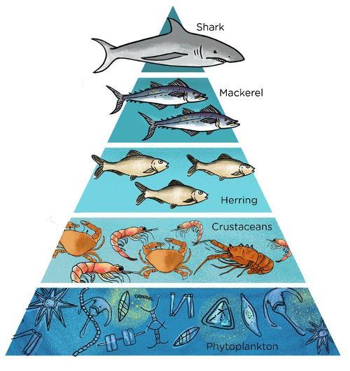
So, how does mercury end up in a shark and ultimately on our plates. Well, it all begins at industrial wastes, mining wastes as well as minerals that naturally contain mercury. Then deposition such as rain, snow and gases can carry the mercury into aquatic environments or the mercury itself, can be seep through the ground and reach water supplies underground. Once it reaches a lake or a river, it will turn into methylmercury by the bacteria. Later, the fish will absorb this through either their food or the water and because mercury cannot exit the fish or other animals, as, it bounds to the proteins in the fish tissues, it can also bio magnify, which is the building up of substances as it increases up the food chain.
Effects of Mercury
Mercury can have various negative effects on our human body, being toxic to our central and peripheral nervous systems. It can also interfere
59
with “cognitive thinking, memory, attention, language and fine motor skills, (World Health Organization, 2017).” Furthermore, at high levels it can permanently damage the brain and kidneys and our skin; it is also thought to be linked to cerebral palsy.
Referencing
World Health Organization 2017, Mercury and health, viewed 13 November 2022, <https://www.who.int/newsroom/fact-sheets/detail/mercury-andhealth>.
Wikipedia 2022, ‘Flake (fish)’, wiki article, 9 September, viewed 12 November 2022, <https://en.wikipedia.org/wiki/Flake_ (fish)>.
How does mercury get into fish n.d., DEC, pdf, viewed 14 November 2022, <https://dec.vermont.gov/sites/dec/fil es/wmp/SolidWaste/Documents/alittl ebit.pdf>.
USGS 2018, Mercury Contamination of Aquatic Environments, viewed 14 November 2022, <https://www.usgs.gov/specialtopics/water-scienceschool/science/mercurycontamination-aquatic-environments>.
60
Where have the Sharks Gone?
Sydney Parker (Year
9)
The Illawarra Grammar School, 10/12 Western Avenue, Wollongong, NSW, Australia, 2500
Sharks, we all know them. We have all heard the eerie jaws theme playing and instantly felt a chill run down our spines, we have all seen the movies with a sharks enormous jaw eagerly waiting to gobble down the smaller fish and even people and we have probably all had nightmares where a shark is chasing us while we are swimming at the beach. It's pretty clear to see that sharks are ingrained in our minds as the greatest killer in our waters, one of the most fear-inducing animals alive but are they really as big a threat as we think, is there existence actually helping us and our environment and are we actually more of a threat to them than they are to us. Each year around 10 people are killed by sharks which doesn't really seem like a lot, especially in comparison to 110000-300000 sharks we humans kill in a single hour. Now a new study has revealed that 90% of the world's shark population no longer exists so it begs the question, What are we doing to sharks and what species of sharks are the most affected.
Whatishappeningtosharks?
Sharks play an integral part of maintaining the balance within marine life as they are at the top of the marine food chain. This balance between marine life is now becoming jeopardised as the shark populations around the world are in rapid decline. There are many reasons that shark populations are declining but the most significant cause is the lack of management of shark fishing. The demand for shark fin is also of great concern as research has indicated that around 100 million sharks may be killed annually for their fins, most of them killed and their fins used to create an expensive asian delicacy known as Shark Fin Soup. There are many other reasons for the decrease in shark
populations though these are two of the most prominent. There are also many different causes affecting individual species and types of sharks. Until recent years these shocking discoveries were often ignored and still are today, this is mostly due to the stigma around sharks.
StigmaaroundSharks
Though sharks are more often the victim, society portrays sharks as bloodthirsty, savage killers, often defining them as a symbol of fear. Hence whenever we hear the Jaws music we all develop a sense of fear and terror; fear that a merciless shark will come and rip us to shreds. This though is not actually the case. There are many different types of sharks, some ginormous like the ones we see on TV but some are actually quite tiny with the Dwarf Lanternshark only reaching a maximum of 8.3 inches (Seen in source 1).Sharks are also almost always not man eaters with many sharks who accidentally hurt or kill a human only doing so after mistaking them for a prey of a similar size. In comparison to the 110000-300000 sharks we humans kill in a single hour, it appears that sharks are the longtime victim of a stigma that has categorised them as vicious killers.
WhichSharkspeciesaretheworstaffected?
A 2021 study conducted by Australian Marine Conservation Society revealed that 37.5% of the world’s shark and ray species are at risk of extinction with 99.6% of the 1093 shark and ray species being threatened by overfishing. The species worst affected are the Daggernose Shark, the Sawback Angelshark, The Striped Smoothhound, The Pondicherry Shark, The Ganges Shark and the Northern River Shark who are all critically endangered according to Ocean Scuba
61
Dwarf Lanternshark- Shark Sider n.d.
Dive 2020, MOST ENDANGERED SHARKS IN THE WORLD. Most of these shark species have also decreased by upwards from 90% and some are considered virtually extinct. The famous Great White Shark also holds a vulnerable status in regards to their endangerment, this is believed to be largely due to overfishing.
Whatarepeopledoingtohelpandhowcanwe help?
WWF and many other conservation organisations working to regulate shark fishing and monitor shark populations. They are working to help fisheries around the world to responsibly manage shark fishing and distribution. They are also fighting to reduce illegal and unsustainable practices within fisheries around the world. They are also fighting for responsible trade and responsible consumption of sharks. Another thing that WWF is doing to help sharks is tracking sharks. WWF supports research and monitoring of white sharks as they migrate to and from the Gulf of California. Sharks are tagged and the movements are tracked by satellite. This information on their behaviour will help with a management plan for the protected area where they are found (Guadalupe Island Biosphere Reserve), such as how to protect them from bycatch and to regulate tourism (WWF n.d., Shark). We can help sharks by both reducing our environmental footprint and by reducing or stopping our consumption of sharks.
In summation, with the knowledge that 90% of the world's shark population no longer exists and the fact that each year around 10 people are killed by sharks whereas 110000-300000 sharks are humans killed in a single hour we should think about whether Sharks are the monster or are they the victim. To help save our sharks we should stop our consumption of the animal that maintains the balance within marine life and take action in order to save the sharks.
Australian Marine Conservation Society 2021, Nearly 40% of world’s shark and rays threatened with extinction, new study reveals, viewed 12 November 2022, <https://www.marineconservation.org au/nearly-40-of-worlds-shark-and-raysthreatened-with-extinction-new-studyreveals/>.
Ocean Scuba Dive 2020, MOST ENDANGERED SHARKS IN THE WORLD, viewed 12 November 2022, <https://oceanscubadive.com/mostendangered-sharks-in-the-world/>.
Shark Sider n.d., The 10 Smallest Species Of Sharks, viewed 12 November 2022, <https://www.sharksider.com/10smallest-species-sharks/>.
WWF n.d., Shark, viewed 10 November 2022, <https://www.worldwildlife.org/specie s/shark#:~:text=Overfishing%20and% 20illegal%20fishing%20of,and%20sur veillance%20of%20many%20fisheries >.
WWF n.d., Shark Facts vs. Shark Myths, viewed 12 November 2022, <https://www.worldwildlife.org/stories /shark-facts-vs-shark-myths>.
Bibliography
62
The effect of increased carbon dioxide levels in water on acidity
Saxon Parrish (Year 9)
The Illawarra Grammar School, 10/12 Western Avenue, Wollongong, NSW, Australia, 2500
Aim
The aim of this experiment is to investigate the effect of carbon dioxide, produced by a neutralisation reaction, on the acidity of water.
Introduction
Ocean acidification occurs in Earth’s oceans when carbon dioxide dissolves in sea water and increases the acidity of the water (Smithsonian Ocean, 2018). Carbon dioxide is created by many human practices that have emerged in the last two hundred years since the industrial revolution. According to World Resources Institute (2017), carbon dioxide is created primarily by creating energy (72% percent of carbon dioxide emissions), which consists of electricity, transport, heating, unaccounted emissions, manufacturing and construction. Carbon dioxide goes into the atmosphere where 50 percent stays (K. Krajick, 2017), and twentynine percent goes into the ocean. Some of the carbon dioxide is consumed by phytoplankton but the remainder is absorbed into water where it increases water acidity. The carbon dioxide combines and reacts with dihydrogen monoxide (water) to make carbonic acid. Carbonic acid that can then dissociate into a singular hydrogen ion (H+) and bicarbonate (HCO3 -) (National Oceanic and Atmospheric Administration, 2020). This is not healthy for the ocean, because acidity of liquids is measured by the amount of free Hydrogen ions relative to hydroxide ions where more hydrogen ions mean more acidic (Khan Academy, n.d.). The more acidic water can then mix with the water deeper then it so deep water will become more acidic but at a slower pace because water takes time to mix. This process has resulted in pH changes of
oceans by 0.1pH (on a scale of 14 where 0 is most acidic) in the last 200 years, despite the small number this means ocean water has become 26 percent more acidic (Woods Hole Oceanographic institution, 2022). It is an increase this large in acidity because the pH scale is logarithmic, a change from 7-8 is 10 times more acidic and a change from pH7- pH9 is 100 times more acidic (see image 1). Changes in acidity from the ocean’s regular and previous pH of 8.1, will hurt sea life: Skeletons can’t be created as easily compared to the normal pH of 8.1 since the hydrogen ions that are free in the water bond with carbonate to form bicarbonate. The carbonate is bonding with hydrogen rather than calcium which would have form calcium carbonate that is important when building bones in marine creatures. The effect of this is that the creatures will dissolve other shells or use more energy making skeletons than in not as acidic water. Shelled animals like mussels and clams will grow 25% less by 2100 (Smithsonian ‘Ocean’, 2017). Corals also make themselves with calcium carbonate, and as a result, a more prone to erosion, destroy other corals to create themselves, become less unique and more rounded to survive when weaker. Two negatives of this effect of ocean acidification on coral, is that marine animals do not have as many places to live where they are safe from predators and tourism opportunities will become less frequent with less appealing coral reefs. Also, some species of zooplankton responsible for removing carbon dioxide from the atmosphere will become extinct is areas across the world, that will make the problem of ocean acidification larger with more carbon dioxide in the atmosphere. Furthermore, fish that live in more acidic ocean water will experience effect in the pH of blood because they are in contact with water. The water will also cycle through their gills so more work will be required to keep the more acidic water from effecting their body systems that cannot cope with changes in pH. Marine animals and creatures will also be slow to adapt to less basic (more acidic) water because they have spent
63
millions of years adapting tolive in pre-industrial revolution waters. In truth, it has been 55.8 million years since the pH of ocean water was this low during Palaeocene Eocene Thermal Maximum (PETM) where organisms went extinct, in the deep sea too (L. Haynes, 2020). This can potentially happen again if human behaviour continues this way without change. However, the PETM likely because of fries spreading around the world and active volcanoes. Ocean acidification can recreate this period in earth’s history without action will kill off many marine animals which is not only unethical but will ruin the earths ecosystem until it is not healthy to live in our environments. However, the purpose of this experiment is to find out if carbon dioxide genuinely does affect the pH of water, and potentially find a relationship between amount of CO2 in water (that will represent ocean water) and acidity. Discovering these results will highlight the urgency of this problem rather than finding a solution.
Hypothesis
Based of the above information and reasoning it is hypothesised that the acidity of the water will increase (decrease in pH) when the amount of sodium bicarbonate reacted increases, therefore, producing more carbon dioxide that is directed into the water.
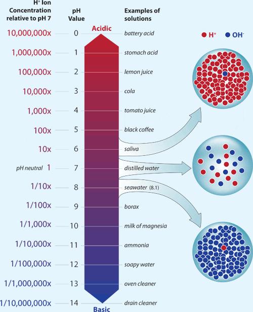
Methodology
Equipment list
• 3 balloons (1 to use and 2 spare)
• 500mL container of white vinegar
• 150g of sodium bicarbonate
• 250mL Filter flask/ flask with side arm
• Pipe attachment that can attach/screw onto filter flask side arm
• 2x Beaker 500mL (measuring beaker and beaker for water)
• 100mL Beaker
• Teaspoon
• Completely charged pH probe
• Scientific weighing scale
• Stopwatch
• Funnel
• Smart Phone
• Water available on tap
• Paper towels
Method
1. The pipe was tightened onto the filter flask using the screw attaching feature.
2. The scale was plugged in to a power point and turned on.
3. 50mL of vinegar was measured out in the measuring beaker, so the bottom of the meniscus was in line with the 50 mL measurement, then poured into the filter flask slowly to ensure no splashing or spillage.
4. 200mL of water was poured into the water beaker using a tap and the pipe connected to the filter flask was submerged in the water.
64
Image 1: PH scale with pH of sea water (USEPA, 2022)
5. The pH probe was turned on, connected to a phone using vernier graphical analysis app (or other app/website that links to a pH probe), taken out of its storage solution and placed in the beaker of water so it did not tip the beaker. The pH probe was left to adjust to the pH of the water for 2 minutes.
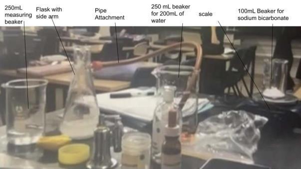
6. The 100ml beaker was placed gently onto the scale and the tare button was pressed to reset the scale weight so the measured weight was 0 with the beaker on top. (The setup looked like diagram 1)
7. The first amount of sodium bicarbonate (5g) was weighed by placing it into the 100mL beaker, using the teaspoon.
8. The 5 grams of sodium bicarbonate were then poured into the balloon using the funnel and the sides of the beaker were scraped using the cleaned teaspoon until there was no sodium bicarbonate in the 100mL beaker. The funnel was flicked softly so the sodium bicarbonate fell into the balloon.
9. The balloon was placed on top of the filter flask by stretching the mouth of the balloon, so it covered the top of filter flask without tipping sodium bicarbonate into the vinegar. This was achieved by squeezing the long/thinner part of the balloon or holding the part of the balloon with sodium bicarbonate pointed downwards.
10. The record button on the pH probe app was pressed, the balloon was tipped over, and shaken/rubbed to empty it for 5 seconds. Simultaneously, the stopwatch was started.
11. After 1 minute and 30 seconds the pH of the water was recorded.
12. The water beaker and filter flask were emptied. The filter flask was then
washed out with water and dried using paper towels.
13. The pH probe was turned off and placed back into its storage solution for 1 minute.
14. Steps 2-13 were repeated 2 more times for the 5g amount of sodium bicarbonate
15. Repeat steps 2-13 3 times for amounts of 10g and 15g.
Controlled Variables
Type of vinegar
Vinegar can differ between different companies and types. Different vinegars do not have the same acidity because there will be different ingredients and different ratios of acid to water. Cooking vinegars like red/white wine and balsamic vinegar are made from fruits like grapes and will not be as acidic as other vinegars. Alternatively, industrial vinegar is more acidic than other vinegar because it is made with 20-30 percent acetic acid and 70-80 percent water. To keep the acidity of the vinegar the same Cornwell’s White Vinegar will be used for this experiment, it is 5-10 percent acetic acid.
Time each before pH is recorded
The time from when the sodium bicarbonate is tipped into to when then pH is recorded must be kept the same because of the sensitivity/slow
65
Diagram 1: Setup of flask with side arm/filter flask, water beaker, pipe and sodium bicarbonate weighing
reaction time of the pH probe and the possibility that, when more time is allowed, the water will become more acidic because the carbon dioxide will have more time to mix with the water. The pH probe takes time to adjust to a change in pH because it is only tuned to detect small changes in pH quickly and accurately. This reduces the speed the pH probe can respond to changes in pH by 1 or 2 because it is designed to ensure it is still recording the right numbers when the pH is changing. This will be controlled by keeping the time, before the pH is recorded, at 2 minutes for every repeat. This time was chosen because it was the amount of time taken for the pH probe to stabilise when being transferred from its storage liquid to tap water when designing the experiment.
Type of water
Different types of water will have different acidities/alkalinity (level of basicness). Acidity and type of water is dependent on water is dissolved in the water and what is taken out of the water. Different types include sea water, tap water, filtered water and freshwater. Sea water has salt mixed into it and a pH of 8.1 because of the minerals mixed into the salt that is mostly sodium chloride. Sea water can potentially have organic matter in it as well. Tap water has chlorine added to it to disinfect the water and kill microorganisms so it is suitable for drinking. Filtered/pure water, has impurities such as chlorine removed and has a pH of 7. Freshwater has no salt but impurities such as organic matter in it. For example, if both salt water and pure water were used in an experiment, results could have a difference of 1 pH between the two water types only because of the base water. In this experiment tap water was used because it was the easiest to obtain.
Amount of vinegar
Vinegar amounts need to be kept the same to prevent occurrences where vinegar will become a limiting reagent in some repetitions/tests but not all. If there is not enough vinegar for the
sodium bicarbonate to react with the vinegar will become a limiting factor (reagent) and stop all the measured sodium bicarbonate from being reacted with. If this happens, the amount of carbon dioxide produced will be less compared to other tests of the same amount of sodium bicarbonate, and consequently, make the water less acidic. 50mL of vinegar was used because it resulted in the amount of vinegar being large enough to react with the sodium bicarbonate every time.
Dependent variable
The dependent variable is the acidity of the water that the carbon dioxide is being directed to. This is because it is representing the change that happens in oceans around the world when carbon dioxide is absorbed by water making it more acidic. It will be measured using a pH probe, because it is the most accurate way of recording pH, it can determine pH in decimals. The alternate method is a pH indicator and pH strip. However, this method only determines pH to a whole number, and it requires human judgement to determine pH which is subjective and inaccurate.
Independent variable
The independent variable in this experiment is the amount of carbon dioxide produced in the reaction between vinegar and sodium bicarbonate (NaHCO3). However, this carbon dioxide cannot be measured so it will be measured as sodium bicarbonate in grams. More sodium bicarbonate will equal more carbon dioxide produced because there will be a bigger reaction when there are more reactants.
66
Results Effect of Amount of Sodium Bicarbonate on acidity of Water Acidity of water (pH) Amount of Sodium Test 1 Test 2 Test 3 Average
The reactions taking place with more sodium bicarbonate as a reactant, that create more carbon dioxide made the water more acidic by a pH of 0.21 between 5 grams and 10 grams and made the water with being pumped with the carbon dioxide produced 15 grams of sodium bicarbonate record a lower pH by 10g by 0.31. There was an outlier, in the third test of 5 grams. The pH of that test had a higher pH by 0.59. This was approximately 43 percent less change of pH from the starting pH of water at 7.
Discussion
The results above prove that the effect of carbon dioxide on water is that the pH will be lowered, and acidity increased. This result supported the hypothesis. The effect of the CO2, produced by the reaction between sodium bicarbonate and vinegar, that could be seen as bubbling in the beaker of water, on the acidity was consistent between tests, excluding outliers. This proves that there is a relationship between amount of carbon dioxide produced and the acidity of water that can be measured. However, in this experiment the amount of carbon dioxide combined with the water could not be determined.
The relationship between carbon dioxide and acidity is negatively linear. This relationship dictates that an increase in 5g of sodium bicarbonate would result in a decrease in pH by approximately 0.25 and an increase of 10 g would increase the pH by two times the previous
increase, and an increase of 15 by three times. This is partially because of the limiting reagent ((“the limiting reactant is the reagent to be totally consumed in a chemical reaction) (ChemTalk, n.d.)) of sodium bicarbonate. All the sodium bicarbonate is reacted before the vinegar and stops the reaction at that point. As a result, this makes the amount of carbon dioxide produced, and consequently the change in acidity/production of carbonic acid, related to/limited by the amount of sodium bicarbonate. It is also because there can only be two hydrogen ions produced per carbon dioxide molecule added.
Seen in the above equation, when carbon dioxide initially mixes into water it dissolves and becomes an aqueous solution with water. Then it will form carbonic acid with water. The carbonic acid will then partially dissociate into ions. It can dissociate into a hydrogen ion (H+) and a hydrogencarbonate/bicarbonate polyatomic ion (HCO3 -). The bicarbonate ion can further dissociate into 2 hydrogen ions and a carbonate ion (CO3 2-) (see image 2) (S. Barker, A. Ridgewell, 2012). The increase in free hydrogen ion in the water make the pH of the water lower and more acidic. H+ lowers the pH because the pH scale classifies liquids based on the amount of free hydrogen ions in the liquid compared to hydroxide ions (OH-). A greater number of hydrogen ions compared to hydroxide ions means that the liquid is acidic with the opposite applying when liquids are classified more basic. In this experiment the water became more acidic by a pH difference of close to 1, meaning the combination of released more hydrogen ions so there were ten times more than hydroxide ions.
67 Bicarbonate (g) 5 5.65 5.65 6.26 5.65 10 5.42 5.42 5.48 5.44 15 5.12 5.16 5.11 5.13
CO2 (aq) + H2O(l) → H2CO3 (aq) Carbon dioxide + Water → Carbonic Acid
This assessment was not valid. There were problems in the method and errors in the way the method was conducted that resulted in the experiment not being valid, also there were problems where different solutions would have minimised the effect of the problems better or make the problem ineffective. Firstly, an outlier by a pH of 0.6 without recognising any error in the method is an indication that there was not enough control and little reliability in the conduction of the method. It was likely, that this was caused by too little vinegar making vinegar the limiting reagent when the limiting reagent is sodium bicarbonate or was caused by the vinegar not being changed over correctly or the change of vinegar being forgotten. Because this happened, it revealed that an instance of vinegar effecting the experiment, when it should not, could have happened at other points in the experiment on a smaller scale. For example, this could be responsible for the results that are difference in pH by 0.08 when it was assumed to have been an error in reading. The results could have also had the slight variations because the experiment was not time correctly. In later stages of the experiments, where the results are noticeably more varied, the reaction was not timed, and the pH was recorded when the water stopped bubbling. The time taken to stop bubbling would be different for each amount of sodium bicarbonate because the reaction would last longer when there are more reactants. Also,
this method requires human judgement, which is inaccurate because it is subjective.
A way of measuring out the bicarbonate soda that would be more valid is to measure the mass of the sodium bicarbonate in the balloon. Pressing the tare button when the balloon is on the scale, then funnelling bicarb directly into it would eliminate the technique of scraping the beaker. This method was not valid because it always left some sodium bicarbonate on the sides of the beaker. Measuring in the balloon would give an exact mass of the amount of sodium bicarbonate that will be reacted instead of the mass of the sodium bicarbonate that could potentially not funnel into the balloon. However, using the balloon as method of pouring sodium bicarbonate also made the experiment more invalid because it left an unknown amount of sodium bicarbonate in the balloon, even after rubbing it and shaking it. A better option is to have a container with an opening that can drop the sodium bicarbonate. Adding another step to the method of checking/calibrating the scale at times during the test would make the method more accurate. The scale could have been checked to see if items weighed the same amount at different points during the experiment. This would have improved accuracy because the masses recorded weight will be closer to the true weight for every test.
The pH probe that used was sensitive and was always flicking between two measurements that had a difference of pH0.01 – pH0.03. There could potentially be pH probes that don’t do this. However, the best solution would be to choose a range (e.g., pH 5.14-5.12) that stayed consistent for all results. The better solution would be to choose the lowest of the pH’s that the probe flickers between and stick with that for every result. This would remove the unpredictability of the pH that shows when the timer is done.
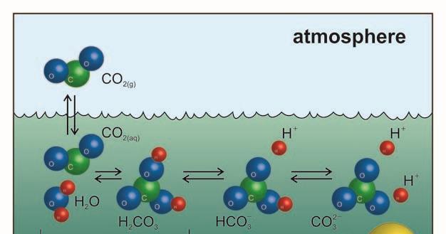
68
Image 2: The process in which carbon dioxide dissolves and becomes carbonic acid, bicarbonate and carbonate (S. Barker, A. Ridgewell, 2012).
Increasing reliability of the test by adding more repeats/tests for each different amount would solve the problem of flickering pH probe and the possibility that the method was not carried out correctly each test. With more repeats outliers could have been located easier as the real range was tested. The averages would also better represent the different results and be affected less by results that are spaced far out. 5 repeats would the optimum amount because it is time efficient and solves the problems. Finally, this experiment did not represent realworld ocean acidification correctly. The pH of water was different to oceans, the combination of carbon dioxide and water happened rapidly, and other differences. These problems could be solved but is unnecessary because the relationship was still discovered without them and because the experiment could be completely changed.
Conclusion
The aim of this experiment was to investigate the effect of carbon dioxide produced by a reaction between vinegar and sodium bicarbonate on the acidity of water and it the hypothesis stated that the more carbon dioxide the more the acidic the water became. It was found that the hypothesis was supported, the acidity increased/pH decreased when CO2 increased. The graph showed that the relationship is a negative linear relationship between carbon dioxide and pH of water. The results and experiment could have been more accurate if times correctly and a better method for reading and recording pH probe measurements was decided on. This experiment connects to the real world because climate issues are taking over the world. Ocean acidification will kill and negatively effect marine animals and environments. Human jobs (fishing and tourism) and the earth’s climate will be affected because of ocean acidification. This experiment helped that cause because it increases understanding on why oceans are being acidified and the effects that will have on the earth.
References Barker, S & Ridgewell, A 2012, Ocean Acidification, Thenatureeducation, viewed 23 October 2022, <https://www.nature.com/scitable/kn owledge/library/ocean-acidification25822734/#:~:text=Carbonic%20acid %20rapidly%20dissociates%20(splits,3 )>.
Center for Climate and Energy Solutions n.d., Global Emissions, viewed 20 October 2022, <https://www.c2es.org/content/intern ationalemissions/#:~:text=Globally%2C%20t he%20primary%20sources%20of,72% 20percent%20of%20all%20emissions>
.
ChemTalk n.d., Limiting Reactant and Limiting Reagent, viewed 25 October 2022, <https://chemistrytalk.org/limitingreactant-reagent/>.
Khan Acadaemy n.d., Acids, bases, pH, and buffers, viewed 22 October 2022, <https://www.khanacademy.org/scienc e/biology/water-acids-and-bases/acidsbases-and-ph/a/acids-bases-ph-andbufffers>.
National Oceanic and Atmospheric Administration n.d., Ocean acidification, United States Government, viewed 19 October 2022, <https://www.noaa.gov/education/res ource-collections/ocean-coasts/oceanacidification#:~:text=Water%20and%2 0carbon%20dioxide%20combine,2%2 0dissolving%20into%20the%20ocean>
.
Unites States Environmental Protection Agency 2022, Understanding the Science of Ocean and Coastal Acidification, United States Government, viewed 20 October 2022, <https://www.c2es.org/content/intern ationalemissions/#:~:text=Globally%2C%20t he%20primary%20sources%20of,72% 20percent%20of%20all%20emissions>
69
Can old milk help plants grow?
Chrissie Cheung (Year
10)
The Illawarra Grammar School, 10/12 Western Avenue, Wollongong, NSW, Australia, 2500
Discussion
How would you deal with the milk which expires in your fridge? I bet you will throw it immediately without hesitation. I believe you will think about what else can do with the expired milk. We can’t drink it as it will make us feel sick, what can we do other than throw it away? Some living creatures need them, the plants in your home! In this investigation, the aim is to grow plants faster in a short period of time but at the same time, provide the best nutrients for the plant. Other than having a healthier plant, this may reduce leftover products. Can decrease the amount of food waste. Therefore, the result supported this theory of giving out more healthy nutrients to plants.
Spoiled, expired milk will be more suitable than fresh milk to water the plants. As after the milk has spoiled, the acidity level of the milk will increase which is more beneficial to the plants. As milk goes sour, bacteria convert lactose into lactic acid. The higher acid of milk is more suitable for planting. According to the website, it proves that using expired milk can increase the speed of planting. It may also provide much more nutrients to the plant, as the expired milk, is loaded with calcium, protein, vitamins, and sugars that can help give your plants an added boost and help them grow big and strong. Calcium is one of the most important nutrients for plants, as calcium is responsible for supporting cell walls. If your plant does not have enough calcium, the root tips, young leaves, and shoot tips could have trouble growing. Additionally, calcium is also used in some enzymes to send signals to fire off certain cellular activities. Some blossom end rot has a common issue of calcium deficiency, such as tomatoes,
peppers, carrots, and apples. And this may benefit them from growing. But we have to be aware of whole milk, as the fat is very high and could cause potential issues with soil moisture absorption as well as foul odors.
The result found in this investigation are considered reliable as the result recorded were, that plants watering with water grow approximately 3cm per day but 5cm for plants watering by expired milk mixture. On day 5, the height of the plants gave out an obvious difference which both also grow faster than in the first 4 days. Beans water with milk was approx. 20cm tall meanwhile, beans with water is just only 15-16cm tall. This result does match the theory of using expired milk mixture for growing plants is faster than only using water.
The results are valid, control variables such as, temperature, it maintains at around 30-35 degrees for the past 2 weeks and the weather condition was mostly sunny and gives out a warm temperature for the plants to grow.
The amount of liquid being watered for the plants may not be as same as the amount every day. Even if I use a measuring cup, the amount may also not be as accurate as every day’s amount and I didn't use the same batter of milk mixture for the 2 weeks, so the nutrients that were given to the plants may not be similar for the 2 weeks.
The two things that I should improve for this experiment are I should make a large amount of expired milk mixture which can be enough for watering it for 2 weeks but not mixing another mixture for another week. The second thing that I should improve is time. As I only have 2 weeks for doing this experiment, although beans are seeds that can already be plated easily, growing plants that can grow out of fruit can result in a proper result.
70
Conclusion
The aim of this experiment was to determine if expired milk can grow plants faster and healthier and it was hypothesised that using expired milk mixture to water plants can grow plants with a greener leaf color and faster-growing speed. The graph below, it shows the difference in the speed of each plant which waters with a different type of mixtures, and the height of plant water by the expired milk mixture is much growing faster than the plant water with plants. As discussed, the time for growing the plants would be the limitation of this experiment. However, the finding in this investigation is useful for not increasing any food-wasting of expired milk and also can increase the speed and the nutrition given to the plants.
References
Micheal, J 2021, Milk Fertilizer: Is Milk Good For Plants?, viewed 28 June 2022,
<https://www.backyarddigs.com/garde ning/is-milk-good-forplants/#:~:text=You%20can%20safely %20water%20plants,you%20apply%20 to%20plant%20foliage.>.
TIMESOFINDIA.COM, T 2020, How to use expired milk to grow healthy plants, viewed 28 June 2022,
<https://timesofindia.indiatimes.com/ life-style/food-news/how-to-use-expiredmilk-to-grow-healthyplants/articleshow/77907455.cms>.
SHIFRAH, C 2021, The Smart Thing Thing You Should Do with Expired Milk Instead of Pouring It Down the Drain, viewed 28 June 2022,
<https://www.thekitchn.com/expiredmilk-use-23124888>.
71
Does colour help your memory?
Ella Fennell (Year 10)
The Illawarra Grammar School, 10/12 Western Avenue, Wollongong, NSW, Australia, 2500
Discussion
This investigation, that aimed to determine the effect of a coloured stimulus on memory performance, found that colour did indeed have an effect on memory, however only red and green resulted in a higher memory performance than black (the control). Whilst yellow resulted in having the lowest number of words that were recalled. It was hypothesised that red and yellow would result in a higher memory performance than black as more words would be remembered. Whilst green would result in a lower level of memory performance. Therefore the results refute the hypothesis as red and green equally recorded having the same words recalled followed by black then yellow.
For a stimulus to be better remembered it must attract enough attention of one’s sensory receptors such as sight to allow for deeper processing, that will ultimately result in longer lasting memory (Dzulkifli & Mustafar 2013). This was found, as red due to its more stimulating colour had a higher degree of attention attached to its text therefore allowing for the information to be thoroughly processed in the brain. As a result more words were recalled during the experiment. However, green unexpectedly also had the same level of memory performance meaning that the colour was stimulating more so than yellow and black allowing the brain to better process the information and commit it to memory. Yellow contrary to previous research had the lowest degree of attention attached to it, thus it was not as deeply processed as the other colours. These results correlate with other findings as Dzulkifi and Mustafar (2013) also found that colour did indeed effect memory performance with red also having the highest impact. However, there was a
larger significance between the data in this secondary source. Accordingly, Huchendorf also found there to be little significance between result averages and no correlation between the brightness of the colour and memory performance.
The results found in this investigation are considered reliable as over the 10 trials for each colour, consistent results were provided. For example the data collected for red only varied by 3 words and the biggest difference between two data points provided by the black stimulus only varied by 2. The results that had been gathered are also consistent with several secondary sources of information such as (Dzulkifli & Mustafar 2013) and (Olurinola & Tayo 2015). However there was not as large of a difference between the recall count of each colour compared to the results found in the secondary sources just mentioned, hence the results found also correlate with findings by (Huchendorf n.d.). Indicating that results gathered on this topic can vary.
Furthermore, the investigation that was conducted was valid as it directly answered the aim by manipulating the colour of a stimulus and measuring the number of words recalled as a result of the coloured stimuli. From the data that was collected it was apparent that it refuted the hypothesis, therefore the investigation was able to answer the hypothesis proving its validity. Nevertheless, the methodology (procedure) was able to control variables that may have affected the outcome of the experiment. This was done by using a stopwatch to constantly monitor the passing time as participants were allowed 45 seconds to study the given palm card, a 15 second break where the palm card was taken away and then one minute to write down the words that could be recalled. Also, the exact same palm card must be used for each trial so there was only one card per colour continuedly used throughout the entirety of the investigation. However the validity of the
72
investigation could be further improved if the colours used were all from the same pack and produced by the same company. This would have ensured that each colour follows a similar shade as a green highlighter would have appeared a lot brighter than a yellow pencil whereas it should represent more of a cooler colour
Additionally, the results were accurate as the procedure was followed accordingly and all results were recorded with the best accuracy possible. This was done by counting the number of words recalled on the sheet of paper, writing that result down, then recounting the number of words listed again. Also, the words written down after each trial were checked over with the ones presented on the palm card, to ensure there was no doubling of words or ones that had been written done despite not being present on the given palm card.
Moreover, the experiment could have been improved had there been a separate task replacing the 15 second break. Instead of only allowing 15 seconds after studying the palm card a quick activity such as answering 10 easy mathematical questions such as 12 x 5, would have been more suitable. This would allow a longer gap between studying the words and writing them down. Causing the mind to focus on something unrelated so that when the participant finished the small task and began to write down the words, it would be a truer test as to the true extent of the effect of colour on memory. From here there would be a larger significance in results and the ability to determine what-coloured stimuli results in longer-lasting memory. Also, another improvement that could have been made was the introduction of control groups. Prior to the experiment no questions were directed at any participants as to whether any underlying issues with memory were known. A simple short-term memory test would have provided enough information to sort participants into groups of similar memory performance dependant on the
results from the test. This would have made the investigation more reliable as results found could have been more dependent on the one’s respective memory ability rather than colour.
From here, it is apparent that colours (particularly red )do have an effect on memory which can be implemented into advertising, education andeven simple things such as grocery lists that occur in everyday life. The ability to be more likely to remember a specific item or content is extremely useful and convenient especially for students completing their HSC, where memorisation is needed due to the amount of content in the respective course. Memory is used in everyday life and could benefit many if only exposed to specific colours known to correlate to a high level of memory performance. However, more research is needed to fully understand to what extent colour can affect memory, particularly long-term. This investigation only targeted working/short-term memory, thus research of higher intensity would be the next step into just how far colour can improve or even deteriorate memory.
Conclusion
The aim of this experiment was to determine the effect of a coloured stimulus on memory performance and it was hypothesised that the red coloured stimulus would produce the highest number of words recalled followed by yellow, black then green. The results gathered reveal red and green to have the most positive effect out of the four colours on memory performance, equally recalling an average of 10 words. Black resulted in 9 words being recalled and yellow unexpectedly had the least impact on memory performance with 7 words. As mentioned, the investigation could have benefitted from the use of control groups based on a group’s current memory level and a quick mathematical task could have replaced the 15 second break to prevent participants from going over words in the mind. Nonetheless, the findings in this investigation are necessary for
73
the future of the educational and marketing systems as the ability to increase the chance of the memorisation of a product or content in a lesson could change the way educators deliver their lessons and companies design advertisements. Also, by implementing colour into everyday life such as grocery lists would also change the way people approach work, school, formation of calendars etc. To fully understand the effect colour can have particularly involving long term memory which was not investigated in this investigation will require a higher intensity of research so that the world may further progress and even treat diseases regarding memory.
References
Dzulkifli, M & Mustafar, M 2013, The Influence of Colour on Memory Performance: A Review, viewed 19 July 2022, <https://www.ncbi.nlm.nih.gov/pmc/ articles/PMC3743993/#:~:text=This% 20suggests%20that%2C%20colours%2 0can,%2C%20and%20thus%2C%20b etter%20memory.>.
Olurinola, O & Tayo, O 2015, Colour in Learning: It’s Effect on the Retention Rate of Graduate Students, Department of Science and Technology Education, Olabisi Onabanjo University, viewed 27 July 2022, <https://files.eric.ed.gov/fulltext/EJ10 80132.pdf>.
Huchendorf, L n.d., The Effects of Color on Memory, Melanie Cary, Department of Psychology, pdf, viewed 21 July 2022, <https://citeseerx.ist.psu.edu/viewdoc/ download?doi=10.1.1.590.8217&rep=r ep1&type=pdf>.
Patel, S 2020, The Effect of Color ect of Color, Preference, and the Inter ence, and the Interaction of Color and action of Color and Preference on Shor ence on Short-Term Memor erm Memory, pdf, viewed 28 July 2022, https://digitalcommons.butler.edu/cgi
/viewcontent.cgi?article=1553&context
74
=ugtheses
Does Music Tempo and Genre Effect Risktaking?
Evie Mullins (Year 10)
The Illawarra Grammar School, 10/12 Western Avenue, Wollongong, NSW, Australia, 2500
Discussion
The aim of the personal project was to test if music genre correlated with risk taking behaviour of adolescence between the ages of fourteen and sixteen years. Twenty four students from the year 10 cohort were chosen to participate. They all listened to a fifty second sample of music, that being either; Sample A, Schumann’s Traumenei (Classical) or Sample B, Tears don’t fall by Bullets for my valentine (heavy metal). It was hypothesised that the twelve students who listened to sample A, would be less prone to choosing riskier decisions, than the other twelve students who listened to sample B, who would be more prone choosing riskier decisions.
To test this hypothesis, the Balloon Analogue Risk Task (BART) was used. BART is a computerised measure of risk-taking behaviour. Which models real-world risk-taking situations through the simple frame of balancing potential reward versus loss.
The test was modified to allow the participant to receive a maximum of three pops, until they are out of the game. There was a total of thirty balloons that the participant had to pump. Every pump the participant makes will earn them five cents. The probability of the balloon popping rises every time they choose to pump it. When five dollars is made, the participant will get a lolly snake.

In the results collected from the tests; it was found that the group of students that listened to heavy metal earned double the amount. Compared to the students who listened to classical music. The tests conducted reflected the hypothesis correctly. This led to believe that the risk-taking behaviour links to the beats per minute (BPM) of the music played, and/or the style and overall tone of the music.
The first part of the explanation for the results is the tonality and style. Although the emotions that are felt from music is all subjective. It can be characterised into simple feelings. For example, classical music makes you feel calm and relaxed, this feeling is caused by the dopamine that is released into the body when listening to music. In this case, classical music typically causes the body to produce dopamine to prevent stress hormones. Compared to listening to ‘extreme’ music, such as heavy metal, this can create feelings such as energetic and compulsive behaviour.
The second part of the explanation for the results is the BPM. The BPM of Schumann’s Traumenei (classical) is sixty six beats per minute, compared to Bullets For my Valentine’s
75
Tears Don’t Fall (heavy metal), which it is close to being triple the amount at one hundred and sixty two bpm.
The reasoning is that when a person is listening to music of a higher BPM it increases the heart rate of that person. This may cause them to have lack of focus in their decision-making process. The fast-paced music also leaves the participant wanting more, which is clearly demonstrated through my results. With the only three students receiving more than one snake, were listening to heavy metal.
There have been many studies focused on music tempo and the influence on our actions. Frontiers in Behavioural neuroscience found that tempo has not only a massive effect on attention span, time perception and decision making, but also an effect on someone’s consumption, diet and driving behaviour.
A way this is seen in the real world is through Casinos and the use of background music which is played. According to contactmusic.com, it was noted recently that in casinos when upbeat and fast music was being played, the customers made not only more impulsive decisions but the customers felt pressured and stressed which made it easier for the casino owners to take the customers money. It was also found that twenty two percent of the time that people gambled with fast paced music playing in the background, they ended up winning money from their games.
The effect of fast paced music in casinos is also noted in Blake Wilson’s article, The Importance of Background Music in Gambling Establishments. Wilson states that fast paced music increases the rate of gambling, as well as the amount of money spent gambling. Wilson also states that the fast-paced music creates a sense of urgency with the customers, which convinces them to gamble faster.
As noted in the results above, the experiment was completed twenty four times in total and Twelve times for each sample size. The experiment was controlled by keeping the experiment testing time from 8am-1pm. Keeping the age of the volunteers between fourteen and sixteen years of age and keeping the length of the music samples the same. As well as keeping the amount, of students in the room to the minimum and having equal number of females and males.
Although all these controls were in place the amount of students in the room would commonly be disturbed, due to the easy access and the knowledge of a prize. This may have affected the early results greatly, due to the risk of peer pressure, but this only happened a few times during the tests.
The main problem with the accuracy of the results was the way in which the results were recorded. The results were recorded by the amount of lolly snakes the student earnt, because one lolly snake is worth five dollars earnt. This created a big gap in accuracy, meaning it was difficult to tell how much money the student earned exactly. It could be anywhere between five dollars to nine dollar and ninety five cents. To fix this, the recording of the results would be the total amount of how much the student earnt and how long it took the participant to finish.
To extend on the findings of this task, it would be interesting to discover whether music of the same genre but different tempo would affect risk taking behaviour of individuals.
Conclusion
The aim of the research task was to find if music genres of heavy metal and classical with varying tempos had an effect on risk-taking behaviour. Of individuals between the ages of fourteen and sixteen years. It was hypothesised that the individuals who listened to heavy metal would
76
take more riskier decisions compared to the individuals who listened to classical.
In conclusion, the results reflected the hypothesis correctly. The individuals who listened to heavy metal music, collectively made more than double than the individuals who listened to classical music. This was most likely because the individuals who listened to heavy metal music took the risk to try to get more lolly snakes. In total, there was only one main problem to the task, that being the recording of the results. The results were recorded by the amount of lolly snakes the participant earned, because one lolly snake is worth five dollars earnt. This created a big gap in accuracy, meaning it was difficult to tell how much money the students earned exactly.It could be anywhere between five dollars to nine dollar and ninety five cents. To fix this, the recording of the results would be the total amount of how much the participant earn and how long it took the participant to finish.
With gambling being so common in today’s society, perhaps music could be a way to either enhance or diminish the amount of money spent on gambling.
77
Georgie Spikoski-Lancaster (Year 10)
The Illawarra Grammar School, 10/12 Western Avenue, Wollongong, NSW, Australia, 2500
Discussion
This investigation aimed to determine whether the dominant hand influences memory perception capabilities. The experiment was conducted to prove the hypothesis that left-hand people had better memory function capabilities. The experiment saw that both left-handed and right-handed participants were tested with number memory and worded memory test to study how the effect of hand dominance. The results from the experiment revealed that lefthanded people have a higher average score of 7. 8 out of 12 compared to right-handed people who had an average of 7.1 out of 12, in the worded component of the testing. Furthermore, left-handed females scored almost 2 points higher than left-handed males indicating a higher memory recall ability.
The results from the number memory test, display those right-handed participants had a high average of 10 out of 18 compared to lefthanded participants 8.8 out of 18. Unlike the worded memory test, both males and females scored around the same point depending on the dominant hand. The results supported the hypothesis as left-handed participants scored higher in worded memory testing, rather than number memory testing.
The experiment aims to provide credibility to the myth that "lefties have better memories". This reiterates the idea that the right side of the brain controls the left side of the body and vice versa. In theory, the idea of left-handed dominant people having an enhanced memory is partly correct as memory is stored and created in the right temporal lobe, however, it is the interconnectedness with the corpus callosum that creates the high functioning memory ability.
The brain lateralisation, functions performed by distinct regions of the brain, allows the corpus callosum to communicate and send signals back and forth to control the body hence performing memory recall abilities. The corpus callosum plays a vital role in cognition within the brain which influences the ability to recognise and understand situations. Therefore, the dominant hand is only a factor that contributes to memory recall ability, as the connectedness between hemispheres allows for the greatest ability to perform.
Since the corpus callosum connects the two hemispheres, the brain sends signals to communicate. When faced with something to remember, the brain forms memories, which reactivate neurons in the temporal lobe. To form memories, some changes take place in the strength of the connections between neurons. During the testing, this process took place within each of the participants, overall affecting how well they scored. Left-handed participants proved to have more enhanced memory in worded memory testing. This is because, as researchers have now identified, the brain of lefthanded dominant people appears to communicate more effectively compared to right-handed people, which may give them an enhanced ability in language and verbal tests.
The results that were discovered from this experiment can be considered reliable as the tests were repeated with different participants, both left and right-handed. With more than one left and right-handed participant, the results can be averaged and analysed more reliably.
The experiment and results were valid. The method provided for both experiments allowed each participant to score, overall displaying the memory ability for each test. However, the accuracy of this test is limited as the number of left-handed participants was limited, hence, this is only used as a sample of tests.
78
If you’re left handed, does it mean your memory is better?
One thing that could improve the experiment would be the environment in which all the tests were conducted. Many of the tests were completed in different areas, either outside, in the classroom, or in a quiet area. The area in which the test takes place can influence the concentration level during the tests. The participants who took the tests in the classroom may have been distracted from the surrounding noise and/or people. This environment is very different from the quiet surroundings where some participants were able to fully concentrate.
This experiment aimed to discover whether handedness influences memory ability, it was hypothesised that left-handed participants would be more successful in performing memory recall abilities. The data indicates that the hypothesis was correct, left-handed participants averaged higher than right-handed participants in memory recall abilities, this is because lefthanded people have a greater connectedness between brain hemispheres. The accuracy of the data could be improved by making sure the environments were consistent throughout all the experiments. The findings of the experiment are important as it looks further into the myth of left-handed people have better memories.
This study concludes the theory of "cross-wired brain function" is inconclusive as left-handed, who historically have higher right-sided brain perceptions, have greater ability to access both sides of the brain, hence having more memory capability in writing and worded tests.
79
What could make one susceptible to contracting COVID-19?
Laura Ellis (Year 10)
The Illawarra Grammar School, 10/12 Western Avenue, Wollongong, NSW, Australia, 2500
Discussion
The aim of the experiment was to investigate the correlation between a number of factors such as gender, level of fitness, length of sleep (on average) and covid susceptibility, and the hypothesis stated that men are more susceptible to getting covid than women. The results that were collected did not support the hypothesis. However, due to the many limitations of the experiment, the hypothesis cannot be rejected, when other research supports the hypothesis. Through this research, there have been two main theories as to why men are more susceptible to COVID, although not enough research has yet been conducted to confirm either way.
The first theory states that men are more vulnerable to getting COVID due to behavioural differences and lifestyle choices. A recent study conducted in Spain, one of the most heavily affected countries in Europe, revealed that women have a ‘more responsible’ attitude towards COVID than men (de la Vega et al. 2020). This may reduce the number of men undertaking preventive measures such as wearing masks and stay at home orders, which potentially affects the higher number of men getting COVID as opposed to women. A study conducted amongst 1050 Bangladeshi adults by Population Medicine (Sultana et al. 2022) revealed that not only were men less likely to take preventative measures than women, they showed a higher tendency to believe in myths about COVID than women, for example more men than women believed COVID could not spread in warm weather (Sultana et al. 2022). This change of approach from men increases the likelihood of men catching COVID
The second theory is based on genetic and immunological differences. The ACE2 receptor is a protein on many different cells (This enzyme generates smaller proteins by cutting up angiotensinogen, a larger protein, which then regulates cellular functions. The SARS-CoV-2 virus (the name of the virus that causes COVID19, part of the broader coronavirus family (UK Research and Innovation, 2020)) binds onto the ACE2 receptor using their interlocking surfaces, before entering and infecting cells. Therefore, ACE2 can act like a cellular doorway for the COVID-19 virus (Sriram, Insel & Rohit Loomba 2020). Much research is still being conducted on the ranging levels of ACE2 in people, but men have a higher concentration of plasma ACE2 than women according to a survey undertaken by European Heart Journal (Sama & Voor, 2020) that looked at thousands of patients in 11 European countries. Therefore it can be predicted that genetically, men are more predisposed to getting COVID, however more research must be conducted on a larger range of subjects to confirm this.
This experiment was limited in reliability since the results did not support the hypothesis and other research. This elucidates a range of uncontrolled variables that had the potential to affect the results. These variables include, but are not limited to, the level of exposure, the health level of participants, the honesty of the survey answers, the variation of coronavirus and any health conditions. There were variables that were controllable which assisted the reliability of the experiment, such as age (all participants were 14-16), species, and place of residency (the Illawarra). Ultimately, the experiment cannot be considered valid since it is unlikely to be repeated if undertaken again.
Overall, the experiment was highly accurate since not only were the questions easily answerable and unambiguous (e.g. have you had COVID - yes or no), they were multiple choice
80
with clear answers for participants to pick from. However, the accuracy could still have been affected by inaccurate answers by participants.
The experiment was overall reasonably valid since the results clearly state that there does not appear to be a correlation between gender and the likelihood of an individual getting COVID, effectively answering the hypothesis. Although the results refuted the hypothesis, neither can be discarded due to the lack of research in this area and the limitations in the reliability of the experiment and any other experiments undertaken.
This experiment could have been improved by increasing the scope of the experiment. This particular experiment was limited with 40 respondents, a tiny amount compared to the millions who had or have COVID, decreasing the reliability of the experiment. A next step could be to roll out this survey to a much larger number of people, with a larger range in age, health level, exposure levels and living conditions to determine whether there is an enduring connection between gender and the susceptibility of an individual towards COVID when these other factors are inconsistent.
Another next step in this investigation could be to evaluate the remaining factors that were surveyed such as sleeping time and exercising rates. Initially, research should be conducted on each of these factors to form a hypothesis. The date collected should then be analysed and evaluated to answer the hypothesis. This has the potential to determine other possibly correlating factors that contribute to an individual’s risk in getting COVID, highly valued during this stage in the COVID-19 pandemic.
Conclusion
The aim of this experiment was to investigate the possible correlation between a number of factors and an individual’s susceptibility to COVID-19.
The factors investigated were gender, hours of sleep each night (on average), amount of exercise, eye colour and hair colour. The hypothesis was that men were more susceptible to getting COVID. Contrarily, the results from the experiment suggested there was no correlation between gender and vulnerability to COVID-19. Opposingly, other research (see discussion) supports the hypothesis, however not enough research has been conducted to prove either way. This experiment had many limitations, including the small number of respondents, the difficulty of controlling experimental variables such as exposure levels, and the contradiction of the results and other experiments conducted. However, results could still assist in the scientific community’s developing understanding of the COVID-19 disease and how to identify and protect vulnerable members of the community. Any research is valued due to the recent and unexplored nature of the disease, and correlating factors in contracting COVID-19 are key to the treatment and prevention of the disease.
References
Adults in Bangladesh: A cross-sectional study’, Population Medicine, vol. 4, no. January, pp. 1–11, viewed 4 August 2022, <http://www.populationmedicine.eu/ Gender-differences-in-knowledgeattitudes-and-npreparedness-to-respondto-COVID-19,145763,0,2.html/>.
De la Vega, R, Ruíz-Barquín, R, Boros, S & Szabo, A 2020, ‘Could attitudes toward COVID-19 in Spain render men more vulnerable than women?’, Global Public Health, vol. 15, no. 9, pp. 1278–1291, viewed 4 August 2022, <https://pubmed.ncbi.nlm.nih.gov/32 623959/>.
Sama, IE & Voors, AA 2020, ‘Men more vulnerable to COVID-19: explained by ACE2 on the X chromosome?’, European Heart Journal, vol. 41, no. 32, pp. 3096–3096, viewed 4 August 2022,
81
<https://academic.oup.com/eurheartj/ article/41/32/3096/5861742>.
Sriram, K, Insel, P & Rohit Loomba 2020, What is the ACE2 receptor, how is it connected to coronavirus and why might it be key to treating COVID-19? The experts explain, The Conversation, viewed 4 August 2022,
<https://theconversation.com/what-isthe-ace2-receptor-how-is-it-connected-tocoronavirus-and-why-might-it-be-key-totreating-covid-19-the-experts-explain136928>.
Sultana, MstS, Khan, AH, Islam, MdR, Hossain, S, Tasdik Hasan, M & Sikder, MdT 2022, ‘Gender differences in knowledge, attitudes and preparedness to respond to COVID-19 among The Covid-19 effects on societies and economies | News | Wellcome 2021, Wellcome, viewed 4 August 2022, <https://wellcome.org/news/equalityglobal-poverty-how-covid-19-affectingsocieties-and-economies>.
UK Research and Innovation 2020, What is coronavirus? The different types of coronaviruses, Ukri.org, viewed 4 August 2022,
<https://coronavirusexplained.ukri.org /en/article/cad0003/>.
WHO Coronavirus (COVID-19) Dashboard 2022, Who.int, viewed 4 August 2022, <https://covid19.who.int/>
82
To cap or not to cap?
Mia Parker (Year 10)
The Illawarra Grammar School, 10/12 Western Avenue, Wollongong, NSW, Australia, 2500
Discussion
The investigation conducted aimed to determine if wearing a swimming cap decreased a swimmer’s 50-meter freestyle time, found that when a swimmer wears a swimming cap, their times begin to decrease in comparison to the times produced when a swimming cap was not worn. Both a column graph and a plot of the two variables indicate the significant difference in both times each swimmer had produced. These results produced consequently supported the initial hypothesis stated.
Competitive swimmers wear silicon swimming caps in order to make them swim faster. Swimming caps do this by keeping the swimmers hair collected together and out of the water in the way of the swimmer. By doing so, the swimmers head is hydrodynamic when the swim through the water. (6 Reasons Why You Should Wear A Swim Cap 2022) When something is hydrodynamic, it means that the motion of water against an object, in this case the swimmer, causes a force to be applied to it creating resistance. The utilisation of a swimming cap reduces this resistance when moving through the water making the swimmer more streamline and hydrodynamic. Swimming caps can also be worn to reduce hair weighing a swimmer down. Water can easily become trapped between individual strands of hair which can cause it to weigh up to 12%-18% more than when it is dry. (How Much Does Your Hair Weigh? 2022)
The results found in this investigation are considered reliable as the times submitted by every swimmer indicates a significant difference in the times recorded (e.g., swimmer 1 - 0.91 milliseconds faster, swimmer 2 – 4.94 seconds faster, swimmer 3 – 2 seconds faster etc). By
repeating the same experiment with 10 different athletes who all produced similar results it can be concluded that the investigation is in fact reliable. The results are also consistent with the secondary sources of information which states that when something is hydrodynamic, it can move much quicker through the water. (6 Reasons Why You Should Wear A Swim Cap 2022)
The results were valid, variables such as different materials of cap were controlled by every swimmer wearing a silicon cap. If the swimmers all wore a cap of different material, it could impact the hydrodynamics that the silicon cap aims to achieve, causing the swimmer to swim slower (Figure 2) E.g., if a swimmer chose to wear a swimming cap made of Lycra, they may have slower times as Lycra is a much more absorbent material in comparison to silicon. When wet, the Lycra cap will absorb water causing it to be heavier and more likely to drag through the water. Water also flows through the Lycra material once an athlete begins to swim. This causes drag and the cap to weigh down the swimmer’s head.
The swimmers all had to swim in a long course pool (50-meter pool) as a short course pool (25meter pool) can produce slower times due to tumble turns being required. By all swimmers swimming in the same type of pool, it enabled the swimmers to submit more valid and consistent times. The aim was able to be answered as the variable of wearing a swimming cap to reduce drag was manipulated and the time taken to swim 50 meters was recorded.
The accuracy of the times being recorded could have been improved as the same timekeeper and stopwatch was not used to record each of the swimmers. To further improve the investigation, all timing could be conducted by the same time conductor with the same stopwatch to ensure consistency and accuracy of the results. Another variable that could affect the results of this investigation is the effort levels of the swimmers.
83
If the swimmers weren’t swimming their hardest, it could have caused a negative impact on the results. The swimmers also all wore their own swimming cap. Another way to make this investigation more accurate would be to have all the swimmers wearing the same cap to ensure consistency and in case any of the caps they were wearing were different from the others.
One factor that could have been improved in this investigation is the inaccuracy of human time keeping. By removing the human factor through using a timing touch pad (Figure 1), the risk of human error can no longer impact the results produced. By implementing this factor in future investigations, the results produced are likely to be more accurate and reliable. This study raises the question, if silicon caps do make a swimmer more hydrodynamic and reduce times, is there another type of cap that can make swimmers even faster? It can also be questioned, how else can the hydrodynamics of a swimmer be manipulated to produce faster times?
mentioned previously, a limitation that could be improved upon if the investigation were to be repeated again is the use of touch pads to record the swimmer’s times to produce more accurate and reliable results, removing the human risk of human error. Despite this, the findings of this investigation were reliable, valid, and accurate. These findings are crucial inorder to understand how wearing a swimming cap could significantly advantage a swimmer in a race by allowing them to become more hydrodynamic and streamline through the water and ultimately causing them to swim faster and produce faster times.
Conclusion
The aim of the experiment was to determine if wearing a swimming cap decreased a swimmer’s 50-meter freestyle time. It was hypothesized that when a swimming cap is worn, the speed at which a swimmer moves through the water will increase and levels of drag will decrease allowing the swimmer to swim at a much faster rate. The results of the investigation support the hypothesis and represent the significant difference in the times of both swims. As
84
Figure 1 - Automatic touch pads used to record swimming times in a race
Figure 2 - Different material swimming caps used by swimmers
Water temperature and its effect on dissolution
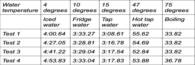 Riley Baird (Year 10)
The Illawarra Grammar School, 10/12 Western Avenue, Wollongong, NSW, Australia, 2500
Discussion
This investigation, which aimed to determine the effect of water temperature on the rate of reaction of Berocca, found that as water temperature increased, the time taken for the Berocca to dissolve decreased. In other words, as the temperature of the water increased, the time taken for the Berocca to dissolve became less. A plot of the two variables showed a clear negative relationship and a line of best fit through the data suggested an overall linear trend. Therefore, the result supported the initial hypothesis. All effervescent multivitamin tablets are designed for one main purpose: to help reduce tiredness and fatigue which can help you wake up in the morning and help to provide an energy high throughout the day. Berocca's work by being a specially formulated combination of high-dose B complex vitamins plus vitamin C and essential minerals, calcium, magnesium and zinc, which work to support your mental sharpness and physical energy throughout the day. (Berocca –frequently asked questions 2019) supports everyday energy release. Helps reduce tiredness and fatigue. The clinically tested formula of 12 essential vitamins and minerals including all the B complex vitamins. Berocca helps to unlock energy from your food so you can be at your best. . The higher the temperature, the faster the molecules move and the more likely it is that the bicarbonate will contact hydrogen in just the right way for the chemical reaction to occur and produce carbon dioxide bubbles as seen in (figure 1).
The results found in this investigation are considered reliable as the results collected were consistent when repeated this is seen when the time for the boiling water was 33.82, 33.82, 33.82 and 36.78 seconds whereas the iced water it took anywhere from 4:00.64 to 4:53.83 minutes which was also seen in table 1.
Table 1, shows the rough times that it took for the Berocca to dissolve) and are consistent with secondary sources of information. (Science Buddies 2013) The results were valid, variables such as room temperature were controlled by conducting the experiment inside on the same day at the same time and ensuring there was an equal amount of water in the cups to control the amount of water the Berocca could make contact with. The aim was able to be answered as the water temperature was changed in tests and the time of rate of reaction was measured. However, the accuracy of ensuring time could be improved

85
Figure 1: The Berocca tablet dissolving in water at tap temperature) (Science Buddies 2013).
as it was difficult to time exactly the moment the Berocca stopped dissolving. although the amount of water in each cup was as close as it could have been better as a measuring jug was used to measure the water, not a measuring cylinder meaning it was not 100% accurate. Two things could be done to improve the experiment. One could use a video camera which could be slowed down to measure accurately the time when the Berocca finishes dissolving. The original size of the Berocca should also be kept the same although this was kept almost completely the same because a full tablet was used there still could have been variations to the tablets. The size of the tablet could be controlled by measuring the weight of the tablet to standardise the same size. The change of size of the tablet was not investigated here but would be worthwhile for further investigation to see if the size of the tablet affects the rate of reaction.
Conclusion
The aim of this experiment was to determine if the temperature of water affects the speed it takes for a Berocca to dissolve and it was hypothesised that the hotter the water the quicker the Berocca would dissolve. When the data were plotted, a clear negative linear relationship was apparent; as water temperature increased, the speed to dissolve decreased due to an increase in particle movement in the water, supporting the hypothesis. As discussed, the accuracy of the findings could have been improved with a better method of timing when the tablet stopped dissolving. Nevertheless, the findings in this investigation are helpful for people who drink Berocca that are trying to find the quickest way to dissolve and drink their Berocca in the morning when in a rush.
References
Are multivitamins different for men and women? | Berocca 2021, Berocca, viewed 4 August 2022, <https://www.berocca.co.uk/theenergy-blog/are-multivitamins-differentmen-and-women>.
Berocca – frequently asked questions 2019, Berocca Australia, viewed 4 August 2022, <https://www.berocca.com.au/faq#:~:t ext=there%20in%20Berocca%3F,How%20does%20Berocca%20work% 3F,physical%20energy%20throughout %20the%20day.>.
Berocca helps your body release energy from food so you can beat fatigue and stay sharp! 2019, Berocca Performance Original Berry Effervescent Tablets, viewed 4 August 2022, <https://www.berocca.com.au/product s/performance/berocca-performanceoriginal-berry-effervescent-tablets>.
Key, JA 2014, Factors that Affect the Rate of Reactions, Opentextbc.ca, BCcampus, viewed 4 August 2022, <https://opentextbc.ca/introductorych emistry/chapter/factors-that-affect-therate-ofreactions/#:~:text=An%20increase%2 0in%20temperature%20typically,for% 20an%20effective%20collision%20(Fig ure.>.
Martin, S 2022, Does Berocca Actually Work? Or Is It A Waste Of Your Money?, Grazia, Grazia, viewed 4 August 2022, <https://graziadaily.co.uk/life/reallife/berocca-actually-work-wastemoney/>.
Science Buddies 2013, Carbonation Countdown: The Effect of Temperature of Reaction Time, Scientific American, viewed 4 August 2022, <https://www.scientificamerican.com/ article/bring-science-home-carbonationtime/>.
86
The Stroop Effect
Samantha Fritsch (Year 10)
The Illawarra Grammar School, 10/12 Western Avenue, Wollongong, NSW, Australia, 2500
Discussion
This investigation, that aimed to determine how cognitive thinking and reaction time is influenced by compatible and incompatible stimulus, found that the congruent condition resulted in a quicker reaction time compared to the incongruent condition. Paraphrased, when the ink colour was matched with the text itself (e.g., red in red ink and blue in blue ink), the response time was more immediate than when the ink colour was not matched with the text itself (e.g., red in blue ink and green in red ink). Therefore, the results supported the initial hypothesis that a congruent stimulus would result in a quicker reaction time compared to an incongruent stimulus.
Cognitive processing can be defined as “taking in information and transforming it, storing it, recovering it, and putting it to work. Such processing allows us to interact intelligently with the world around us”, (Eagleman, 2018). However, when the brain must process a stimulus that displays a contradiction of information, the development of this information takes longer as the mental processes must decipher and determine which section of stimulant should be utilised, hence taking a longer time to process, and thus resulting in a longer reaction time.
There are two types of cognitive processing, these include automatic and controlled thinking. Automatic thinking is a mental process that occurs subconsciously and without any interference, whereas controlled thinking is a mental process that occurs consciously and requires interference and intended thinking. This is heavily related to the Stroop effect due to the link and connection to the Automaticity
theory. The Automaticity theory suggests that “automatic reading doesn’t require focused attention. Instead, the brain simply engages in it automatically. Recognizing colours, on the other hand, may be less of an automated process. While the brain registers written meaning automatically, it does require a certain amount of attentional resources to process colour, making it more difficult to process colour information and therefore slowing down reaction times”, (Cherry, 2022).
Furthermore, the selective attention theory is able to highlight that selective attention chooses “which information will be granted access to further processing and awareness, and which will be ignored”, (Lesley University, n.d.). This is important as there is a limit to how much information can be processed at any given time, with selective attention enabling insignificant details to be ignored. This can help explain the fact that compatible stimulus results in a quicker response time as reading is an automatic response “that occurs without any voluntary effort. This is only true for single words or short sentences but shows how we do not have full control of what we read and how the automatic processes activated by our mind can be in conflict with desired and intentional behaviour”, (Marini, 2018). Hence, identifying the colour of the text takes more attention than reading the text as identifying the colour is not an automatic response, suggesting that the processing of written information is much quicker than processing the colours of text.
This is supported via ‘The Speed of Processing Theory’. This theory states that “the speed with which information can be sensed, perceived, understood and responded to, changes due to the automatic responses of the brain”, (Silva and Lee, 2021). This claims that people can read words at a quicker rate than naming colours as word processing is an automated response while colour processing is a voluntary response. ‘When the incongruent stimulus is recognised, the
87
brain first reads the word, which makes it difficult to then name the colour. As a result, a delay occurs when trying to name the colour as it goes against the brains first instinct and the automated response’, (Ruhl, 2021).
Furthermore, the theory of Parallel Distributed Processing proposes the idea that ‘the brain does not function in a series of activities but rather performs a range of activates at the same time, parallel to each other’, (anonymous, n.d.). Hence, “some of these pathways such as reading words, are stronger than others, such as naming colours, which highlights the interference is not an issue of processing speed, attention, or automaticity, but rather a battle between stronger and weaker neural pathways along with voluntary and automated responses”, (Ruhl, 2021).
These theories can be heavily supported by J.R.Stroop’s original experiment in 1935 that found ‘Subjects also took significantly longer to identify ink colours in experiment two than they had to simply read the printed word in experiment one. He identified this effect as interference causing a delay in identifying a colour when it is incongruent with the word printed’, (Lesley University, n.d.).
The results found in this investigation can be considered reliable, since collected results were consistent with the overall averages for males, females, and overall, (e.g., in set 3 of the data which measured the reaction time of incongruent stimulus showed compatibility, with the average male reaction time being 7.668 seconds, average female reaction time being 7.95 seconds and the average overall 7.809 seconds). Additionally, the results collected were consistent and supported by secondary sources of information including ‘C.Ruhl, 2020’, ‘Lesley University, n.d.’ and ‘J.R.Stroop, 1935’.
The results were valid as variables such as the participants, the test set of words and age group
were controlled. The age group was controlled as reflexes and responses made to stimulus tend to slow with age. “Physical changes in nerve fibers slow the speed of conduction and parts of the brain involved in motor control lose cells over time”, (University of Rochester Medical Centre, 2022). Controlling the test set of words, ensured that the results were kept valid as the participants were reacting to the same stimulus and hence the reaction time would be similar. Further, keeping the participants the same for each set of testing enabled valid results to be collected as a difference could be calculated from each partaker. The aim was answered as different forms of stimulus (incompatible and compatible) were utilised to see the difference in reaction time via manipulating the type of stimulus and hence the response made by the participants. As there were also the same number of males and females used throughout the experiment this ensured there was no gender-biased collection impacting the results. However, the accuracy of each participant's reaction time could be improved as it was challenging to precisely time the exact starting and end time of each set of words. Errors in timing due to a delay in the start and conclusion of the test set were difficult to avoid as the timer could not precisely start and stop the stopwatch when the set of testing was concluded or initiated.
Two main things could be done to improve the experiment. Using online software on a computer could be utilised in order to accurately measure the starting and stopping time of each participant’s response. This would ensure that the results show a more accurate trend as human error would be removed. Furthermore, the testing should have been administered in the same environment this should have been in a quiet area that was detached from any visual or auditory distractions. Not conducting the experiment in the same space with the same conditions may have impacted the response time of a number of participants due to the difference
88
in setting which may have caused a distraction, acting as a hindrance to the speed of cognitive thinking and processing. Using a larger sample size and expanding the demographic of the participants, in particular, age group would result in the experiment being more reliable and therefore not an overall generalisation of findings.
To improve this investigation further, a wider age range should be utilised to increase validity as age may influence cognitive thinking and in turn reaction time. This was not used throughout this experiment but would be beneficial to both discovering the relationship between stimulus type and reaction time along with the relationship between age and how this impacts cognitive thinking and response time.
Conclusion
The aim of this experiment was to investigate how different types of visual stimulus (incompatible and compatible) impact cognitive processing and in turn response time. Once the data was collected, it was found that congruent stimulus results in a quicker response time compared to an incongruent stimulus-response time. As discussed, the accuracy of the finding could have been improved via a better method of timing, achieved by utilising online software. Nevertheless, the finding in this investigation is important to understand as it highlights the essential and necessary functioning of cognition, while also highlighting how automated and voluntary responses impact response time along with thinking/processing mental speed.
References
A Quick Look at Reflexes 2020, University of Rochester Medical Center Rochester, New York, viewed 20 July 2022, <https://www.urmc.rochester.edu/enc yclopedia/content.aspx?ContentTypeI
D=1&ContentID=562#:~:text=Reflexe s%20do%20slow%20with%20age,great ly%20from%20person%20to%20perso n>.
Cherry, K 2022, How the Stroop Effect Works, Very well mind, viewed 18 July 2022, <https://www.verywellmind.com/whatis-the-stroop-effect-2795832>.
Eagleman, D 2018, Cognitive Processing: What It Is and Why It’s Important, Brain Check, viewed 18 July 2022, <https://braincheck.com/articles/cogn itive-processing-what-it-is-whyimportant/>.
Marini, M 2018, The Automatic Mind, Psychology today, viewed 18 July 2022, <https://www.psychologytoday.com/au /blog/the-hidden-mind/201812/theautomaticmind#:~:text=Cognitive%20automatici ty&text=The%20answer%20almost%2 0certainly%20is,occurs%20without%2 0any%20voluntary%20effort>.
Ruhl, C 2020, The Stroop Effect, Simply Psychology, viewed 17 July 2022, <https://www.simplypsychology.org/str oop-effect.html>.
Silva, M & Lee, J 2021, Processing Speed, Science Direct, viewed 17 July 2022, <https://www.sciencedirect.com/topics /biochemistry-genetics-and-molecularbiology/processing-speed>.
Stroop, J. R. (1935). Studies of interference in serial verbal reactions. Journal of Experimental Psychology, 18(6), 643–662. https://doi.org/10.1037/h0054651
The Parallel Distributed Processing Approach n.d., viewed 19 July 2022, <https://www.massey.ac.nz/~wwpapajl /evolution/assign2/AA/paraproc.html #:~:text=The%20Parallel%20Distribut ed%20Processing%20(PDP,time%2C %20parallel%20to%20each%20other>
What the Stroop Effect Reveals About Our Minds
n.d., Lesley University, 29 Everett St, Cambridge, MA 02138, viewed 18 July 2022, <https://lesley.edu/article/whatthe-stroop-effect-reveals-about-ourminds#:~:text=In%20relation%20to% 20the%20Stroop%20effect%2C%20th e%20brain%20likely%20reads,than%2 0we%20can%20process%20colors>.
89
Fractional Distillation: how we get different oils
Sarvani Thapaliya (Year 11)
The Illawarra Grammar School, 10/12 Western Avenue, Wollongong, NSW, Australia, 2500
Crude oil is a mixture of hydrocarbons and is a relatively volatile liquid. “A hydrocarbon is an organic compound, consisting of only hydrogen and carbon atoms” (Clark 2018). Hydrocarbons are group 14 hybrids, meaning they contain atoms from the carbon 14 group. Crude oils can also be categorised into the most prevalent type of hydrocarbon it is composed of: refinery gases, petrol, naphtha, kerosene, diesel oil, fuel oil and bitumen. These hydrocarbons along with many others which exist in crude oil which are useful in different industries. Paraffins are the most common hydrocarbon in crude oil and are highly valued, as they are a major component of gasoline. Naphthenes are an important constituent of liquid refinery products and aromatics (while only a small percentage of crude oils) are in common use in the petrochemical industry (crude oil | Definition, Characteristics, & Facts | Britannica 2022). The separation of these substances are of vital importance, as they are capitalised on in separate industries.
Fractional distillation is designed to separate mixtures of two or more liquids which have differing boiling points. The column is set up such that substances with lower boiling points are collected before those of higher boiling points, as shown in the diagram above. The process involves heating the mixture, resulting in the collection and condensation of vapours along a fractionating column. The vapours condense onto a tray once they reach the part of the fractionating column which is cooler than their boiling point and bubble caps help to slow the vapours as they rise through the column. Any residual gases from the bottom of the column pass through holes in the tray and lighter hydrocarbons still present in the condensed liquid boil off and rise through the column (Energy Institute, n.d.). This method is generally used when the difference of boiling points between the substances is less than 25 °C (New World Encyclopedia, 2017).
While undergoing fractional distillation, crude oil separates into the following hydrocarbons: bitumen, fuel oil, diesel oil, kerosine, naphtha and gasoline (paraffins come under bitumen) (Fractional distillation - Energy Education 2020)). Aromatics are benzenes, which are a base component of gasoline (Burroughs 2015).
As hydrocarbons exist as covalent bonds (intramolecular bonds), there are also intermolecular forces between molecules, which are significantly weaker than intramolecular bonds. The intermolecular bonds in hydrocarbons are known as London dispersion forces (which only exist in non-polar molecules) and they are the weakest of the intermolecular forces. “They are attractions of molecules that only exist within a short period of time” (Khan Academy, 2015). A liquid boils at the point of enough energy to break these intermolecular bonds, therefore the amount of intermolecular forces in a molecule is directly proportional to the amount of energy required to break those forces.
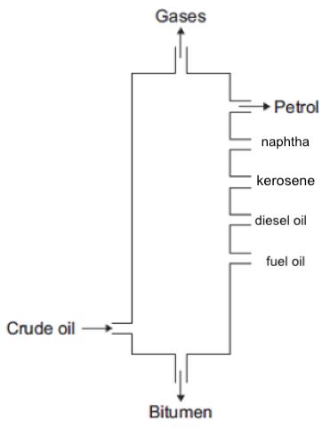
90
The length of hydrocarbon chains and the force of intermolecular bonds between the hydrocarbons explains the difference in boiling points between hydrocarbons. As shown in the diagram above, the refinery gases have the lowest boiling point out of the different hydrocarbons in crude oil. The different hydrocarbons in crude oil contain differing amounts of carbon atoms: gases contain 5-10, naphtha contains 512, kerosene contains 10-16, diesel oils contains 14-20, fuel oils contain 20-70 and bitumen (residue) are substances contain a carbon chain longer than 70 carbon atoms (which are nondistillable) (Energy Institute, n.d.). Larger hydrocarbons have a larger surface area, meaning that there are more opportunities for London dispersion forces to occur, resulting in increased attraction between the molecules of hydrocarbons. Henceforth, the heat energy required to break those bonds will increase (Khan Academy, 2015).
References
crude oil | Definition, Characteristics, & Facts | Britannica 2022, Encyclopædia Britannica, viewed 12 March 2022, <https://www.britannica.com/science/ crude-oil>.
Clark, C 2018, What are hydrocarbons? - Gulf Coast Environmental Systems, Gulf Coast Environmental Systems, viewed 12 March 2022,
<http://www.gcesystems.com/what-arehydrocarbons/>.
Fractional distillation - New World Encyclopedia 2017, Newworldencyclopedia.org, viewed 14 March 2022,
<https://www.newworldencyclopedia.o rg/entry/fractional_distillation>.
Fractional distillation - Energy Education 2020, Energyeducation.ca, viewed 26 March 2022,
<https://energyeducation.ca/encyclope dia/Fractional_distillation>.
Burroughs, D 2015, Growing Chorus of Complaints on Chemicals in Gasoline, Morning Consult, Morning Consult, viewed 26 March 2022,
<https://morningconsult.com/2015/0 4/22/growing-chorus-of-complaints-onchemicals-ingasoline/#:~:text=Aromatics%20are% 20a%20base%20component,well%20t he%20fuel%20actually%20works.>.
Khan Academy 2022, Khanacademy.org, viewed 27 March 2022, <https://www.khanacademy.org/scienc e/chemistry/states-of-matter-andintermolecular-forces/introduction-tointermolecular-forces/v/boiling-pointsof-organic-compounds>.
Marek Lichtarowicz 2014, Cracking and related refinery, Essentialchemicalindustry.org, viewed 27 March 2022, <https://www.essentialchemicalindustr y.org/processes/cracking-isomerisationandreforming.html#:~:text=The%20refine ry,damage%20to%20a%20car%27s%2 0engine>.
Fossils into fuels. Processing crude oil - refining 2022, Schoolscience.co.uk, viewed 27 March 2022, <http://resources.schoolscience.co.uk/ EnergyInstitute/1416/fossils/p8.html>.
91
Fractional Distillation
Loren Yusuf (Year 11)
The Illawarra Grammar School, 10/12 Western Avenue, Wollongong, NSW, Australia, 2500
How and why fractional distillation is used
Fractional distillation is the process of separating a mixture of liquids into different fractions using their boiling points. Fractional distillation is a process completed at a large scale by oil refineries to separate crude oil into more useful components for gas, fuel, plastic products, waxes, waterproofing and much more. All these components are hydrocarbons and can be refined to create various products from crude oil once they have been separated. Hydrocarbons are chemical compounds made up of covalently bonded hydrogen and carbon atoms, which can have different amounts and configurations of these atoms (Boechler et al.)
As seen in figure 1, crude oil is heated and pumped into the distillation tower. The tower is sectioned, with the sections higher up in the tower getting cooler, allowing hydrocarbons with lower boiling points to rise higher up through the tower and condense at distinct levels. This separates the hydrocarbons into fractions that contain other hydrocarbons with similar; numbers of carbon and hydrogen atoms, boiling points, ease/ability to ignite, and viscosity (difficulty for a substance to flow). Gasoline or petrol separates into the range of C5-C12 carbon atoms and has a boiling point of 20-70°C. This allows it to be separated from gases such as butane and propane (C1-C4 and <40°C), and naphtha (C12-C16 and 70-160°C).
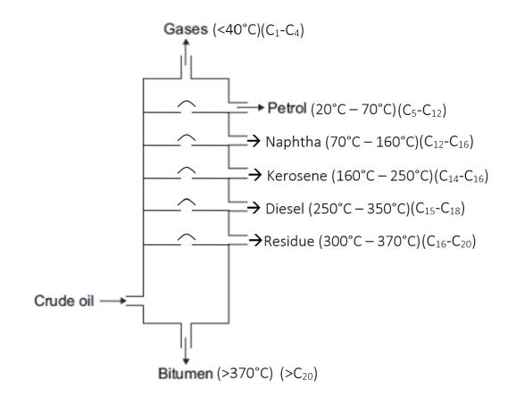
Carbon atoms and boiling point
The number of carbon atoms in a hydrocarbon affects the boiling point due to intermolecular forces, specifically Van der Waals’ Forces. Van der Waals’ force is the theory that if the electrons of an atom were paused at any moment, there would be more on one side of the molecule than the other, creating a temporary dipole moment. The dipole then attracts the electrons of a neighboring molecule, thus strengthening the intermolecular force. Thus, the more carbon atoms there are bonded together, the more electrons there are, increasing the number of attractive forces acting on the molecules. This is reflected through the increased boiling point because more energy (in the form of heat) is required to overcome the intermolecular forces and separate the mixture into individual molecules. Figure 2 illustrates this relationship, showing the increase in boiling point as the number of carbons increases. The line begins to curve near the end of the graph because as the overall molecular weight increases, the percentage increase of the carbon’s molecular weight becomes less effective and has slightly less effect (although still significant) on the boiling point.
The reason intermolecular force and boiling point is dependent on the carbon and not the hydrogen is because of the size of the molecules/their molecular mass. Van der Waals force is dependent on the size of the atoms because a larger atom has more electrons, hence,
92
Figure 1.
it can have a greater imbalance in charge and thus, require more energy to overcome the intermolecular force. Therefore, because hydrogen only has one electron, it cannot have a noticeable impact on the intermolecular forces attracting the molecules to one another and requires additional carbon atoms to increase intermolecular force.
<http://www.passmyexams.co.uk/GCS E/chemistry/alkanes-physicalproperties.html>.
References
BBC 2022, Separating crude oil - Crude oil, hydrocarbons and alkanes, BBC Bitesize, viewed 20 March 2022, <https://www.bbc.co.uk/bitesize/guide s/zshvw6f/revision/3>.
Boechler, E, Hanania, J, Jenden, J, Stenhouse, K & Donev, J 2020, Fractional distillation, Energy Education, viewed 2 March 2022,
<https://energyeducation.ca/encyclope dia/Fractional_distillation>.
McCord, P 2019, Chembook - Crude Oil Refining, Texas, viewed 20 March 2022,
<https://mccord.cm.utexas.edu/chemb ook/pagenonav.php?chnum=5§=7#topofpage>.
Pass My ExAms - Chemistry 2020, Physical
Properties of Alkanes, Passmyexams.co.uk, viewed 20 March 2022,
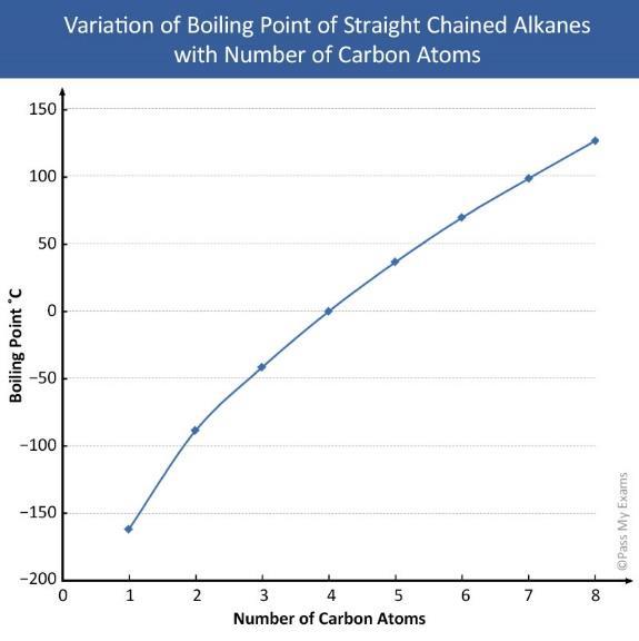
93
Figure 2. (Pass My ExAms - Chemistry 2020)
The Effect of Drop Height on the Coefficient of Restitution
Rhiannon Evans (Year 11)
The Illawarra Grammar School, 10/12 Western Avenue, Wollongong, NSW, Australia, 2500
Introduction
Newton’s Law of Restitution states that the velocity of two objects after they collide depends on the material they are made of. The coefficient of restitution represents a material’s elasticity, thus measuring the elasticity of the crash by determining the amount of kinetic energy lost in the collision (Ashish, 2017). The coefficient of restitution is the ratio between the relative rebound and impact velocities of an object which means that it can never have a negative value (BYJU’S, 2021) as the rebound velocity can never be greater than or equal to the impact velocity as per the law of conservation of energy. The law of conservation of energy states that energy cannot be created nor destroyed, only transferred or transformed. Thus, the coefficient of restitution can only ever be between 0 and 1 where a perfectly elastic crash where no kinetic energy is lost would have a coefficient of 1 and a perfectly inelastic collision where all kinetic energy is lost would have a coefficient of 0. Potential energy is the stored energy in an object which can be transformed into kinetic energy. In this experiment, potential energy is transformed into kinetic energy when the ball is dropped. The greater the drop height, the more potential energy exists in the object before release which, when transformed during the descent, means more kinetic energy exists in the object upon collision.
This experiment aims to investigate the effect of the height an object is dropped from on the coefficient of restitution upon collision with the ground by increasing the drop height by even intervals. It is expected that the drop height will
have no effect on the coefficient of restitution of an object.
Method
The experiment was set up with two one-meter rulers taped to the wall above each other and the camera was set up at a height of one-metre. The camera was started and stopped after each test. The ball was dropped by the experimenter from the height of 1.5-meters, a process that was repeated 5 times before the drop height was decreased by 0.25-meters. This process was repeated until the drop height on 0.5-meters was reached. Once the tests were complete, the experimenter reviewed the videos to observe the height each ball reached after the collision. The impact and rebound velocities were calculated using the equation v2 = u 2 +2as. The coefficient of restitution was calculated by dividing the rebound velocity by the impact velocity.
Results
The experiment showed a direct relationship between drop height and the impact and rebound velocities. Both the impact (Figure 2) and rebound (Figure 3) velocities increased as drop height increased, though the impact velocity increased at a slightly faster rate. An inverse relationship between the drop height and the coefficient of restitution was also shown. As the drop height increased, the coefficient of restitution lowered by a small amount.
94
Effect of Drop Height on the Coefficient of Restitution
experiment by Harden, Petersen, and Taylor. Moreover, this trend is supported by the fact that a greater drop height would give the object more time to transform potential energy into heat and sound energy which would decrease the amount of kinetic energy both before and after collision.
Evaluation
Discussion
It was hypothesised that the height from which an object was dropped would have no effect on the coefficient of restitution. However, an inverse relationship between the drop height and the coefficient of restitution was shown by the graph. While there was a clear linear relationship between the impact and rebound velocities and the drop height, the impact velocity increased a slightly higher rate than the rebound velocity. This caused the coefficient of restitution to slowly decrease as the divisor in the ratio increased at a greater rate than the dividend.
The results of this experiment are not consistent with what is physically possible, though the trend aligns with the research of others. A linear relationship suggests that the coefficient of restitution would eventually reach zero if a specific drop height was reached. However, it is not possible for the coefficient of restitution to equal zero, thus suggesting that the relationship must be an exponential curve or level off at a minimum value when it reaches a certain drop height as suggested by (Harden et al. 2012). Regardless, the results showed in inverse relationship which was supported by the 2012
The experiment was partially successful in addressing the hypothesis as it proved an inverse relationship between drop height of an object and the coefficient of restitution but failed to prove the shape of the curve that would exist if the experiment was continued to include higher drop heights. The experiment was repeated enough times at each drop height to identify outliers and establish an average. However, the data would have been more accurate if the experiment had been repeated at least four times as many times to get an average closer to that of the theoretical average since the range in values observed was large, and at more heights to properly identify the relationship between the variables.
The control variables in the experiment were the height of the camera when recording the experiment, the coefficient of restitution of the ground the ball collided with, the release of the ball and the straightness of the rulers used to measure the height. The height of the camera remained untouched throughout the experiment which meant that the readings from each height were taken from the same angle, but as the camera was not adjusted as the drop and bounce height lowered, the parallax error throughout the experiment was not consistent. The ball was dropped on the same spot on the ground in each test which meant that the coefficient of restitution of the ground (which was negligible compared to the coefficient of restitution of the ball) remained the same throughout the experiment. The ball was released by the experimenter (one person) each time which limited but did not eliminate differences in the release style and also meant
95
Figure 1: The effect of increasing drop heights on the coefficient of restitution.
y = -0.0899x + 0.9713 0.000 0.100 0.200 0.300 0.400 0.500 0.600 0.700 0.800 0.900 1.000 0 1 2 3 Coefficient of Restitution Drop Height (m)
that human error was present as the ball could never be dropped without interfering with the descent. The rulers used to measure the drop height and bounce height remained untouched throughout the experiment so any offset was applied to all measurements. The combination of the effects of these variables suggests that the experiment results were not valid, though the differences were small enough that the data could still be combined and compared for the purpose of this experiment.
The main sources of error in the experiment were the levelness of the ground the ball was dropped on, the quality and angle of the video, the release of the ball, the measurement of the drop height when setting the ball to be released, and the method of observation of the bounce height.
The ball did not bounce directly upward as it was not dropped straight downwards due to the style of release which was caused by human error and collided with the ground, the levelness of which could not be controlled (Bennett & Meepagala, 2005). The video was of poorer quality meaning that the observations of the bounce height after collision were not captured properly in one frame, thus meaning that the ball was likely observed slightly before or after reaching the maximum height. Moreover, the drop height was not exact as it was estimated by the experimenter which provided opportunity for human error. The equipment used relied on human observation to collect data and did not account for parallax error, this not allowing for accurate measurements as each data point was estimated upon reviewing the videos.
As such, the data from this experiment was exposed to many influences that prevented it from being very accurate, reliable, or valid. The control variables were not properly accounted for and the reliance on human observation and movement meant that the data collected was not precise, nor the experiment carried out identically each time. However, the data did present a relationship between the drop height
and the coefficient of restitution, thus satisfying the aim of the experiment.
To improve this experiment, the use of electronic data loggers and mechanical releases would be advised to reduce the reliance on human capabilities, thus dramatically reducing the room for error. Wind should also be accounted for as it could affect the descent of the object used in the experiment. Other factors to consider investigating include air density (for much greater drop heights) and temperature. In conclusion, the drop height has an inverse relation to the coefficient of restitution. It may be exponential or level off at a minimum value for the coefficient of restitution after reaching a specific drop height where it cannot continue to decrease.
96
References
Ashish, 2017, Coefficient Of Restitution: Definition, Explanation, Science ABC, viewed 15 June 2022, <https://www.scienceabc.com/puresciences/coefficient-of-restitutiondefinition-explanation-andformula.html>.
Bennett, J, Meepagala, R, 2005, Hypertextbook, viewed 25 July 2022, <https://hypertextbook.com/facts/200 6/restitution.shtml>.
BYJU'S, 2021, Coefficient of Restitution, viewed 15 June 2022, <https://byjus.com/jee/coefficient-ofrestitution/>.
Harden, J, Petersen, P, Taylor, A, 2012, IB Physics Lab Report, K12.or.us, viewed 22 July 2022, <http://tuhsphysics.ttsd.k12.or.us/Res earch/IB13/PeteHardTayl/CoR.htm>.
Average Rebound Velocity
97
Appendix
Figure 2: The effect of varying drop heights on the impact velocity. The graph shows a positive linear relationship.
y = 2.1148x + 2.2792 0.000 1.000 2.000 3.000 4.000 5.000 6.000 0 0.5 1 1.5 2 Velocity (m/s) Drop Height (m)
Impact Velocity y = 1.4177x + 2.4434 0.000 1.000 2.000 3.000 4.000 5.000 0 0.5 1 1.5 2 Velocity (m/s) Drop Height (m)
Figure 3: The effect of varying drop heights on the rebound velocity. The graph shows a positive linear relationship.
Average
Gravimetric Analysis
Loren Yusuf (Year 11)
The Illawarra Grammar School, 10/12 Western Avenue, Wollongong, NSW, Australia, 2500
Introduction
All matter can be classified into two main categories: non-mixtures and mixtures. While non-mixtures cannot be separated using physical properties, mixtures can use properties such as density, particle size, boiling points, melting points, solubility, and magnetic properties. (Murray, S 2003)
These properties are determined by the structure and bonding of atoms or molecules involved and allow different methods to be used to separate several types of mixtures. Some methods can include sedimentation, sieving, distillation, decantation, filtration, magnetic separation, evaporation, and crystallisation. (McGraw-Hill Australia 2003)
Mixtures can be categorised into a further two sub-categories: homogenous mixtures and heterogeneous mixtures. While homogenous mixtures are single-phase and uniform in composition (i.e., salt dissolved in water), heterogeneous mixtures can have two or more phases of matter and have a variable composition (i.e., sand and water). (Murray, S 2003)
Gravimetric analysis is a form of data analysis scientists use when determining the percentage composition of several components within a mixture. This is done by calculating the weight of each element/component within the mixture and is often represented as a pie chart. An example of its real-world application is when scientists monitor the percentage composition of lead found in water sources to make sure it is fit for human consumption, preventing poisoning and even death.
This makes accuracy incredibly important when calculating the weight of each component. Whilst a theoretical calculation can be made as to the chemical composition of a mixture, there are times when the mixture must be separated to calculate the percentage composition. In these cases, accuracy is extremely important as even just a few grams can significantly impact and change the percentage composition of a component, and in turn, affect the entire gravimetric analysis.
Keeping this in mind, this experiment investigated how the physical properties of a heterogeneous mixture made up of sand, salt, lead, and iron filings can be used to separate it into its components as accurately as possible.
The hypothesis is that the physical properties of each element within the mixture vary, allowing the mixture to be separated to a high degree of accuracy, and result in a gravimetric analysis that reveals the percentage composition to be almost identical to the original mixture. By using the physical properties of each element in the mixture, the most accurate method of separating each component will be by; separating iron filings using the magnetic qualities; lead using the large particle size/density; sand using the lack of solubility in water; and salt using its extremely high boiling point.
Method
The analytical balance was plugged in, turned on and set to grams. Standard masses of 5g, 10g, 20g, 50g, and 100g were placed on the balance, each reading was recorded and used to calculate the calibration curve by plotting it on a graph and applying the gradient to recorded results to provide a calibrated result.
The container containing the mixture of sand, salt, lead, and iron filings was weighed and recorded.
A magnet was used to separate the iron filings from the rest of the mixture; it was placed on one
98
side of a zip lock bag which was used as a barrier from the iron filings. The magnet was used to attract the iron filings which were then placed in a separate container (previously weighed and recorded) by removing the magnet from the bag, using the plastic as a barrier allowing the filings to drop into the container. This was completed several times in the original mixture until no more iron filings were collected. This process was repeated to purify the iron filings, shifting them in small amounts to another container (Department of Education and Early Childhood Development). The separated iron filings and remaining sand, salt and lead mixture were weighed separately and recorded.
The lead was then separated from the remaining sand and salt mixture by placing the mixture into a fine sieve (850µm) with the accompanying tray underneath (Wiki User 2010). The contents of the mixture were spread evenly across the surface of the sieve, and lead shot was picked out and placed into a separate container (previously weighed and recorded) using forceps. The sand and salt mixture were then collected and placed back into the original container, using paintbrushes to ensure no pieces were caught in the sieve. The separated lead and remaining sand and salt mixture were weighed separately, and their results were recorded.
Distilled water was then added to the sand and salt mixture until all salt granules were dissolved. Before being placed in a funnel and beaker, the filter paper was weighed. The saltwater and sand were poured into the filter paper and funnel from the original container. Once the saltwater drained through the filter paper, a small amount of distilled water was used to rinse any remaining undissolved salt from the sand before the filter paper and sand were removed from the funnel and placed into a drying oven at 70°C. The sand was dried and weighed five times (left in the oven overnight) to ensure all water had evaporated before recording the final weight.
The remaining saltwater in the beaker (previously weighed and recorded) was placed in the drying oven (also at 70°C) and evaporated slowly until only salt remained. This was taken out and weighed on the analytical balance five times (being left overnight each time) before the final/stable weight was recorded. All weights/measurements were recorded and then calibrated by multiplying the calibration gradient with the recorded weight to receive the true weight. Any calculations of individual components’ weights were made using the calibrated measurements before a gravimetric analysis of the mixture was completed.
Results
Table 1
99
COMPONENT: WEIGHT (g): Experimental Original Error Sand 2.84 2.82 +0.02 Salt 7.56 7.78 -0.22 Lead 5.85 5.95 -0.13 IronFilings 6.22 6.33 -0.11 Total 22.48 22.88 -0.4
COMPONE NT: PERCENTAGE COMPOSITION RELATIVE TO ORIGINAL SAMPLE (%): ERR OR (%): Experime ntal Origi nal Sand 12.41 12.33 0.71 Salt 33.05 34.00 2.83 Lead 25.57 26.01 1.68 IronFilings 27.21 27.67 1.74 Total 98.25 100 1.75
Table 4
Discussion
Overall, the results revealed a high degree of accuracy throughout the experiment, separating the mixture with 98.25% accuracy, and only incurring a small loss of 0.4g, or 1.75% overall. Additionally, the percentage error for each component of the mixture remained below 3%, reinforcing that the separation methods used were appropriate and allowed for high accuracy.
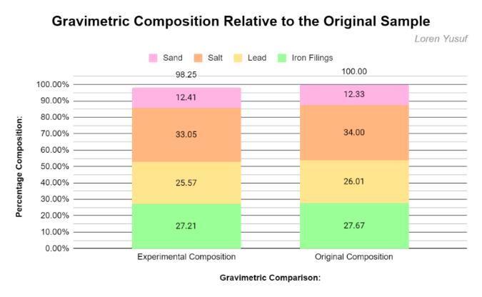
Some factors which could have caused the overall loss of 0.4g could be the handling of the mixture causing accidental loss of material, or random error. This could be mitigated further through careful handling, or storage of all materials in sealed containers to prevent accidental spillage/loss of materials. More specifically, the increased 0.02g of sand can be attributed to either water that remained unevaporated, undissolved salt in the sand, or accidental spillage of sand (from another group/experiment) into this sample. It is highly unlikely to be the first as the sand was placed into a drying oven and weighed five times. Additionally, it is unlikely (but still possible) to be undissolved salt, as the sand was thoroughly stirred in the water, additionally being rinsed once in the filter paper. This leaves the accidental transferal of sand from another sand sample as the potential source of error, as it was transported and dried with sand samples from other experiments which could account for the slight increase in mass. As a result, improvements to the method could include
using warm water to ensure all salt is dissolved, and storing the sand and filter paper in a container when not being weighed to prevent accidental transferral of sand from other samples.
The loss of 0.22g of salt could be explained by undissolved salt remaining in the sand (explained above), salt caught in equipment such as the small holes in a sieve, or salt being lost during transferral between containers. This could be mitigated by using a sieve with finer holes to prevent the salt from getting caught.
The loss of 0.13g of lead could be attributed to slight rounding errors. These rounding errors could be because of the calibrated mass being calculated (explained further below), due to the analytical balance’s systematic errors which were mitigated, or the analytical balance only weighing to two decimal places. Therefore, this could also apply to all other separated materials/components in this experiment and is difficult to mitigate, other than using an analytical balance that shows the mass to more decimal places.
The 0.11g decrease in iron filing mass could have been due to iron filings not being collected magnetically, however, this is unlikely with the mixture being shifted and sought through several times until no more iron filings were able to be collected. This means it is more likely to be rounding errors or calibration.
The iron was able to be separated due to the magnetic properties it exhibits. Magnetism is the property of an atom that is caused by electrons orbiting the nucleus in the same direction. Most elements are not magnetic because they have an equal number of electrons orbiting in opposite directions. Iron, however, has electrons orbiting in the same direction, creating an electrical current and north and south magnetic poles. When two magnetic substances meet, the magnetic fields will cross over, causing the opposite poles of the magnets to attract and
100
1
Graph
creating a larger magnetic field, as seen in figure 2. (Rutledge, et. al, 2011) This allowed the iron filings to be separated using the magnet, while the other substances remained unaffected.

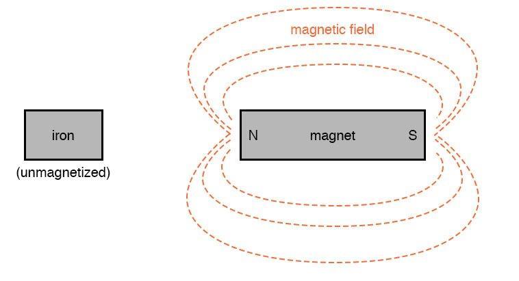
The lead was then able to be separated due to the significantly higher density and particle size. The density of the atom is affected by the number of atoms the substance has in a specified volume. The atomic mass of the element also contributes to its density because the more protons and neutrons an atom has, the greater its mass per atom, therefore, contributing to the density of the substance. (Sciencing Contributor 2017) Further, the lead atoms are metallically bonded to each other. The delocalised electrons create great attraction between the lead atoms, and thus, high density. With lead having a density of 11.29 g/cm3 (compared to salt’s 2.16 g/cm³, and silicon dioxides 2.65 g/cm³), it is easily the densest substance. This enabled it to be separated by swirling/shaking the mixture, causing a separation, and then using forceps to pick out the lead pieces.
The salt was able to be separated using solubility and boiling point. Salt or NaCl is soluble in water due to the polarity and dipole-dipole forces. NaCl is ionically bonded, while water is covalently bonded. In H2O, oxygen is significantly more electronegative than the hydrogens, and the bent geometry of H2O molecules causes the differential in electronegativity to create a permanent dipole moment, and thus, making the molecule polar. This is important because when NaCl is added to water, the water molecules surround the salt and the intermolecular forces overcome the ionic bonds, separating the Na and Cl into individual ions. This is because sodium is a cation, and so the negative dipole in H2O (oxygen) is attracted to it. Similarly, chlorine is an anion and attracts the positive dipoles of H2O (hydrogens). This causes the water to orientate itself around the individual ions and allows the NaCl to dissolve as seen in figure 3. SiO2, however, cannot be dissolved into water. This is due to the “like dissolves like” rule, which states that a solvent can only dissolve a polar substance if it is polar, or a non-polar substance if it is also non-polar. Sand is mostly SiO2, which is a nonpolar molecule, and therefore cannot be dissolved by the polar water.
Further, once the sand was removed, the salt was then able to be separated from the water using the high melting point of NaCl, and low boiling point of H2O. NaCl is bonded in an ionic lattice structure. The opposite charges of the ions create a strong attractive force and bond, requiring substantial amounts of energy to break them, and therefore has a high boiling point (1,465°C). Whereas water is covalently bonded H2O molecules held together by intermolecular forces (including dipole-dipole forces, hydrogen bonds, and van der Waal’s forces). This means that whilst the intramolecular bonds of H2O are strong, the intermolecular forces are weak and require much less energy to overcome, causing it to have a low boiling point (100°C), and thus, evaporating and leaving behind the salt.
101
Figure 2. (Kuphaldt, TR 2015)
Finally, sand was able to be separated from the saltwater due to its insolubility (previously discussed above) and particle size. SiO2 is a covalent network, meaning it is made up of a tetrahedral structure, with each atom being covalently bonded to the surrounding atoms. This causes SiO2 to be a large structure in comparison to the H2O molecules and dissolved sodium and chlorine. This allows filter paper to be used, which allow the much smaller sodium cations, chlorine anions, and H2O molecules through while catching and separating the much larger SiO2 molecules.
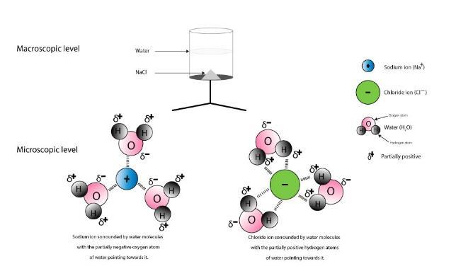
This experiment is valid due to its controlled nature, and a method and results which seek to answer the aim. This experiment sought to minimise and control as many external factors as possible in the method to attain highly accurate results. This includes factoring any potential systematic errors into the experiment’s method, and using the same analytical balance for each measurement.
Further, this experiment was fairly reliable. The results of this experiment align with research conducted on separation methods and physical properties of the substances part of the mixture. The high levels of accuracy obtained in this experiment also contribute to its reliability, however, to further improve, this experiment should be repeated using the same method and equipment several more times to reflect consistency and thus reliability in the method and results.
Finally, this experiment achieved a significant level of accuracy which is reflected by the minimal error in the results. This is not only due to the precise equipment used, but also considerations such as the calculation of a calibration curve (and application to the data) to mitigate the effect of systematic errors on the results. Whilst improvements can be made including previously listed recommendations (such as storage in containers, equipment with greater precision, etc.), the accuracy of the experiment cannot be much further improved.
Therefore, this experiment was extremely effective in investigating its aim. The method was devised and resulted in an extremely accurate, reliable, and valid experiment being conducted. This was further supported by the results obtained and the supporting theory and research behind the method.
References
Department of Education and Early Childhood Development, Separating Iron Filings, Salt and Sand, Primary Connections, viewed 2 March 2022, <https://www.primaryconnections.org. au/themes/custom/connections/assets /SBR/data/Chem/sub/sepironfil/sepi ronfil.htm>.
Edrolo 2021, Chemistry Year 11 (2022, NSW), Edrolo.com.au, viewed 26 March 2022, <https://edrolo.com.au/class/1086907 /studyplanner/>.
Kuphaldt, TR 2015, Permanent Magnets, Allaboutcircuits.com, All About Circuits, viewed 26 March 2022, <https://www.allaboutcircuits.com/tex tbook/direct-current/chpt14/permanent-magnets/>.
McGraw-Hill Australia 2003, Methods of Separating Mixtures, OLLE, viewed 24 March 2022, <https://olle.tigs.nsw.edu.au/send.php ?id=96113>.
Murray, S 2003, Classification of Matter Worksheet, OLLE, viewed 24 March 2022,
102
Figure 3. (Naah, B 2017)
<https://olle.tigs.nsw.edu.au/send.php ?id=96194>.
Naah, B 2017, How does sodium chloride (NaCl) dissolve in water?, Masterconceptsinchemistry.com, viewed 26 March 2022, <https://masterconceptsinchemistry.co m/index.php/2017/10/24/how-doessodium-chloride-nacl-dissolve-inwater/>.
Rutledge, K, Ramroop, T, Boudreau, D, McDaniel, M, Teng, S, Sprout, E, Costa, H, Hall, H & Jeff Hunt 2011, Magnetism, National Geographic Society, viewed 26 March 2022, <https://www.nationalgeographic.org/ encyclopedia/magnetism/>.
Sciencing Contributor 2017, Atomic Number Vs. Atomic Density, Sciencing, viewed 26 March 2022, <https://sciencing.com/differencebetween-density-mass-5529858.html>.
Wiki User 2010, How can you separate a mixture that contains sand sawdust iron filings and lead shot?, Answers.com, viewed 2 March 2022, <https://www.answers.com/chemistry/How_ can_you_separate_a_mixture_that_contains_s and_sawdust_iron_filings_and_lead_shot>.
103
An experimental investigation of drag and noise reduction properties of sharkskin in a low viscous aerodynamic environment
Casey Lockrey (Year 12)
The Illawarra Grammar School, 10/12 Western Avenue, Wollongong, NSW, Australia, 2500
Abstract : In the past decade, research into natural surfaces that outperform those created by man has been on the rise, with potential applications in transportation, military and renewable energy. The surfaces of some organisms, due to the process of natural selection, have evolved due to natural selection pressures in their environment. Sharks, for example, have faced the selection pressure of water density slowing down their movement speed, evolving to possess a unique denticle surface on their skin that reduces drag. This present paper investigates the drag and noise reduction properties of an organic sharkskin denticle coating in a low viscous aerodynamic environment. An evaluation of current literature on the topic is provided along with discussion of the drag reduction mechanism, its effect and an understanding of the developments made in explaining the phenomenon. The drag and noise reduction properties were assessed by measuring the sound and speed of a small DC fan coated in cured organic sharkskin using a microphone and camera. The results indicated a statical difference in noise production (p < 0.05) with a maximum sound reduction of 10 dB seen in the fan with the coating. The rotational velocity remained unchanged due to an unforeseen flaw in the methods design (p > 0.05).
Introduction
In recent times, the utilisation of biomimetic technologies has been explored to address issues with
drag and noise (Tian et al. 2021). One promising candidate is sharkskin and its unique denticlestructured surface.
Denticles are tooth-like microstructures that exist on the surface of sharkskin (See (b) in Figure 1), they are the most significant factor contributing to a sharks’ superior movement in the ocean (Society 2020).
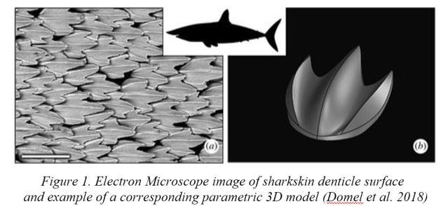
Just like any other object, when sharks move through a fluid, the fluid exerts a force on the shark. This is known as a hydrodynamic force, or if the object is in air, an aerodynamic force (John David, 2016).
The skin of sharks possess tiny rigid scales that effectively delay the occurrence of chaotic fluid movement known as turbulence (green area in Figure 2) by maintaining constant fluid flow known as laminar flow (blue area in Figure 2). This transition from laminar to turbulent flow is called flow separation (pink area in Figure 2) which when delayed (i.e. ��1 <��2 in Figure 2 and 3) reduces pressure drag caused by the lowpressure region near the trailing edge of the object.
104
Figure 2. A circular object undergoing laminar flow. The blue region indicates the area of laminar flow, the pink area indicates the point of flow separation, and the green area indicates the turbulent flow.
This low-pressure region is also primarily responsible for sound generation as sound waves are unable to propagate effectively through the region. This causes vibrations that create noise. Initial research into the drag reduction properties of sharkskin was conducted in 1985 when Reif and Dinsklater (1985) discovered that the morphology of sharkskin scales reduce drag in some turbulent conditions via a force balance wind tunnel and an organic sharkskin coating (Reif, 1985)
Since then, research has been focused on synthetically replicating this surface with testing results showing that this drag force can be increased and manipulated (Tian et al. 2021).
It should be noted that while this flow separation is delayed, that is, the drag reduction mechanism of organic sharkskin, it is not presently understood (Tian et al. 2021). It should be noted that while the concept of flow separation is accepted as common knowledge in literature (John David Anderson 2019), the mechanism of its delay from the organic sharkskin is still not fully understood (Tian et al. 2021).
However, there are still a multitude of studies that have provided important conclusions about the properties of sharkskin and its drag reducing effect (Tian et al. 2021).
Bechart et al. in 2000 investigated multiple biological surfaces with biomimicry potential. The drag reduction of sharkskin was investigated and experimentally proven, for both organic and synthetic sharkskin, via a direct shear force measurement. (Berchart et al, 2000).
Bechart et al. described this drag reduction via “sweeps” and “ejections”. The strong exchange in momentum as the accelerating high-speed flow decelerates whilst approaching the surface (called a “sweep”, A to B in Figure 4) and then accelerates whilst leaving the surface (called an “ejection”, labelled C to D in Figure 4) (Berchart et al, 2000), reducing skin friction as the force applied to the surface is less. This increases the duration of laminar flow and as a result delays flow separation (Berchart et al, 2000).
In 2012 J. R. Debisschop and F. T. M. Nieuwastadt conducted a study to investigate the characteristics of the turbulent boundary layer and the effectiveness of riblets for skinfriction reduction using a drag balance (Debisschop & Nieuwstadt 1996).
The turbulent boundary layer refers to the layer of fluid in the immediate vicinity of the surface of the object and can be inferred to be related to the delayed flow separation (John David Anderson 2019).
The distinctive difference between this study and Berchet et al. is their emphasis on differentiating between the application of riblets in small pressure gradients opposed to medium and large pressure gradients (Debisschop & Nieuwstadt 1996).
The pressure gradient essentially refers to the difference between the pressure at the trailing edge and the leading edge. It’s dependent on the position of the flow separation as the flow separation determines the size of the lowpressure region at the trailing edge and the high-
105
Figure 3 - A circular object undergoing laminar flow with a reduced low-pressure region due to delayed flow separation. The blue region is the low-pressure region.
Figure 4. Graphical representation of the transfer in momentum (Berchart et al, 2000).
pressure region at the leading edge (John David Anderson 2019).
Results from the study indicate that riblet structured surfaces performed better in medium to large (adverse) pressure gradients compared to lower pressure gradients, a maximum drag reduction of 13% being achieved in high pressure gradient regions whereas in lower pressure gradients 6% was achieved (Debisschop & Nieuwstadt 1996).
This suggests that in terms of an air foil or wing, the surface experiencing the largest pressure gradient will benefit the most from the addition of the sharkskin denticle structured surface (Green area in Figure 5).
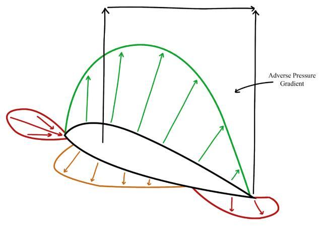
In 2012 Leonardo P. Chamorro investigated the drag reduction properties of sharkskin through studies involving a synthetic replica. The skin was manufactured by 3M © and was tested under different conditions, such as, the angle of attack ranging from 0°≤�� ≤10° and different riblet geometries ranging from 100���� to 80���� in height (Chamorro, Arndt & Sotiropoulos 2013).
that mimics that of sharkskin
The drag was measured via a wake survey and sensitive force balance, it was found that a maximum drag reduction of 6% could be achieved with peaks at a height of 100���� in a “V” shape when �� =0 (See Figure 6) (Chamorro, Arndt & Sotiropoulos 2013).
This study discovered that the transfer in momentum initially proposed by Bechert et al could be manipulated to maximise the drag reduction by minimising the distance over which the momentum transfer occured (Chamorro, Arndt & Sotiropoulos 2013).
In 2018, August G. Domel et al. investigated sharkskin-inspired designs that improved aerodynamic performance in different settings. Additionally, comprehensive CFD simulations and investigations into other surface types were conducted to provide a more comprehensive analysis (Domel et al. 2018).
It was determined that the complex denticle structure seen in sharkskin was not integral to increasing lift and reducing drag at low angles of attack. However, at higher angles of attack, the sharkskin denticle structure performed better (Domel et al. 2018).
This phenomenon was attributed to a short separation bubble forming behind the denticle enhancing this transfer of momentum mentioned in Berchet et al (See Figure 7), resulting in a more consistent drag reduction across all angles of attack.
This provides a more comprehensive explanation compared to Berchet et al. as it was explicit why the transfer of momentum was enhanced, however, in principle both
106
Figure 5. The green highlighted area indicates the adverse pressure gradient (most effective location for the riblet coating), the orange indicates the medium pressure gradient and the red the low-pressure gradient
Figure 6. Simplified diagram of the denticle structure
explanations are very similar.
main peaks seen in the air foil void of modification. (Dang, Mao & Tian 2019). The reduction in noise was attributed to the ‘secondary vortex’, or what has previously been described as a short separation bubble, which maintained laminar flow and hindered the process of turbulence. This separation bubble was described as consuming the energy of the flow and weakening the intensity of turbulent burst (also known as flow separation) (Dang, Mao & Tian 2019).
Scientific Research Question
Will the addition of a sharkskin denticle coating aligned with the direction oflaminar flow reduce the drag experienced and noise produced by an air foil?
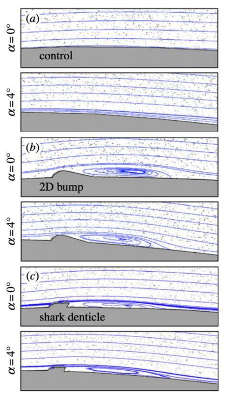
Methodology
Practical Testing
The sound production and speed of the fan void of any sharkskin coating was initially tested as a baseline to compare to the fan with the sharkskin coating.
The specifications of the fan include its design speed of 1200 rpm, the individual air foil dimension being 5.5 cm by 3.4 cm, the propellor radius being 9.5 cm and the angle of attack for each propellor being 20±5�� elevation perpendicular to the direction of flow.
Whilst literature exploring and manipulating the drag reduction potential of sharkskin is well established (Tian et al. 2021), it’s sound reduction potential is under-researched and essentially mute in terms of studies conducted in air. However, other studies have been conducted that investigate the sound reduction potential in other settings such as hydrodynamic environments (Dang, Mao & Tian 2019).
In 2019 Zhigao Dang et al. utilised CFD simulations to predict the hydrodynamic noise of an air foil (Dang, Mao & Tian 2019). This study determined a maximum noise reduction of 7.28 dB could be achieved and that the noise spectra of the biomimetic hydrofoil lacked the
The sound production was measured in 30 second intervals using an iPhone 13 microphone at 120 Hz, 15 cm from the base fan legs. The ambient noise was reduced by closing doors, windows and turning off devices that were creating noise (air conditioning) with the ambient noise initially being measured to ensure it was stable.
The rotational speed of the fan was measured using a 240-fps camera, determined by counting the frames in Adobe Premiere© and calculated using the simple period formula (i.e., �� = 1 ��, where T is the period in seconds and f is the frequency in rotations/second).

107
Figure 7. Flow trails of fluids passing over different surfaces (Domel et al. 2018).
The position of the recording device was crucial as the sound intensity varied with different positions. The microphone was positioned near the ‘outside rim’ of the fan, which is near the trailing edge of the fan blades, as this has been shown to produce the largest amount of noise (Kohout & Hyhlík 2020).
Treatment of the Sharkskin
Sharkskin was obtained in large strips of 30± 10cm from the scraps of a local fish store and used as the source for an organic sharkskin coating, the width and height were ensured to be larger than what was required as the treatment caused shrinking of 10±5% for both the width and height.
The treatment method involved scraping the excess meat off the under-face of the skin using a scalpel followed by curing the skin on a ceramic smooth surface such as a plate for 1.5 to 2 hours in direct sunlight at noon. The skin was dried to a point that made it suitable to handle and rigid before being attached to the fan blades. The rigidity of the sharkskin was crucial to the strength of the adhesion to the surface of the blade, which if not maximised could lead to the sharkskin detaching from the surface during testing.
The skin, after treatment, was cut into 7 by 5 cm squares (to fit the blades with minimal off-cut) and ‘re-wetted’ using a standard clothes iron, separated by baking paper to reduce contamination.

The heat and small amount of moisture from the iron provided a temporary amount of flexibility which was required to form the skin to the curved shape of the blade.
A thin layer of flexible contact adhesive (Selley’s Kwik Grip ©) was applied to the fan blade and spread evenly using a paddle pop stick. The skin was uniformly pressed onto the blade for 10 minutes, with the abrasive direction (the direction in which you would need to move your finger on the surface of the skin to feel friction) facing the same direction at the rotation and the opposite direction to the flow. The skin was left to dry on the blade for 12 hours before being used for testing.
Testing procedures for the fan with sharkskin followed the same protocols as testing the fan without sharkskin.
Statistical Analysis
Statistical analysis was conducted after the data was obtained.
A two-tailed unpaired student’s t-test of equal variances was undertaken tocompare statistically the difference between the noise and speed of both fans. The standard deviation, mean, 95% confidence intervals and F-test were also determined for further analysis.
The utilisation of a two-tailed t-test compared to a one-tailed t-test for the noise and speed of both fans is justified due to an absence in literature to
108
Figure 8. Visual diagram indicating the distance between the microphone and the fan.
Figure 9. Sharkskin being ironed in order to increase flexability
support the initial claim and lack of certainty in whether the addition of the coating would cause an increase or decrease in noise production. The two data sets were compared using an F-test and determined to have similar variances (p < 0.05) and hence it’s also justified to assume equal variances.
Results
Results from the experiment indicate a statistically significant decrease in sound production from the fan covered in the sharkskin and an almost non-existent change in speed.
standard deviation of the fan void of any modification (2.49) was similar to the fan with the sharkskin coating (1.68).
There was however only a slight decrease in the rotational speed of the fan with the sharkskin but was considered not statistically significant as the p value was greater than 0. The mean rpm of the fan without the sharkskin was 1209 rpm and 1196 rpm for the fan with the sharkskin indicating a decrease of 13 rpm. The standard deviation of the speed of the fan with the sharkskin (0.64) and without the sharkskin (0.79) was significantly low indicating that both fans spun consistently at the same speed.
Discussion
Upon initial inspection the results from this investigation clash, as there is a reduction in noise from the addition of the coating but an unchanged rotational speed. This was simply due to a flaw in the experimental design of measuring the speed of the fan. The essentially unaffected speed can be attributed to the design specifications of the fan, limiting the speed at which the fan can operate, which is an unforeseen limitation of this investigation.
The reduction in drag, as described previously, can be attributed to the denticle structured coating maintaining laminar flow and thus delaying flow separation. As a result, the extent to which the low-pressure region can interfere with surrounding air molecules is reduced and hence less noise is generated. This is also described as interactions with the turbulent boundary layer and is found to occur at the trailing edge of an object (Kohout & Hyhlík 2020).
As a result, the null hypothesis that the sound would not change or increase can be rejected as the p value was less than 0.05 and the conclusion that there was a decrease in sound can be made. The decrease in sound on average was 10 dB with the 95% confidence interval of this difference being from 8.6 to 11.4 dB. The
109
Figure 10. Comparison in the noise produced by the fan with and without sharkskin
0 5 10 15 20 25 30 35 40 0 10 20 30 Noise produced (dB) Time (2 second intervals) Comparison
Fan with modification Fan void of modification
in
the noise produced by the fan with and without sharkskin
In the case of sharkskin, it is important to identify what type of drag is being reduced because there are countless unavoidable sources of drag such as those seen in viscous energy losses (John David Anderson 2019).
The denticle structure of sharkskin is primarily responsible for minimising pressure drag by delaying the flow separation. It does this by forming a small separation bubble that consists of vortices. When the fluid collides with these vortices
there is a transfer in momentum that favours the movement of the object, this is because the collision is highly elastic as the kinetic energy of the particle approaching the vortice is close to that of the kinetic energy of the particle leaving the vortice (John David Anderson 2019).
The small separation bubble is formed from the unique curvature of the denticle structure, which when undergoing laminar flow is observed to create these vortices (Bhatia et al. 2021).
The sharkskin, as mentioned in the methodology, was only located on the upper surface of the air foil in support of Debisschop & Nieuwstadt’s conclusion that the sharkskin coating performed better in adverse pressure gradients. A limitation of this study was the lack of resources to produce a 3rd fan model with a coating on both the top and the bottom of the air foil to test Debisschop & Nieuwstadt’s conclusion. This would have provided greater insight into the properties of the surface and contributed to the accuracy of this design decision (Debisschop & Nieuwstadt 1996).
The method used, however, was able to validly indicate whether noise was produced (as indicated by the results), being enhanced (in terms of validity) by the microphones positioning which was supported by literature (Kohout & Hyhlík 2020).
As a further area of study, the use of CFD simulations using software (such as ANYS FLUID©) could allow the comparison of the experimental results to the theoretical results. This comparison would ensure that the results were accurate and in-line with baseline data computed previously.
The extent to which sound reduction occurred at varying distances from the fan was left unexplored due to limited time. This would have provided a better indication on if the observations were in line with other studies such as Dang, Mao & Tian in 2019 which described the noise reduction as weakening with distance (Dang, Mao & Tian 2019).
This investigation did not intend to experimentally prove that the lining of the blades with real sharkskin is a feasible commercial solution to reducing sound production in everyday life, however the findings presented in this paper do suggest that a synthetic denticle coating has the potential to reduce noise production.
Further research could involve synthetically replicating the sharkskin in a manner that is more suitable for an aerodynamic setting such as that experienced by a plane wing or helicopter blade. The results from this paper thus act as a preliminary indication of this sound reduction for further research to use.
This synthetic replication has been seen in a multitude of research papers such as Leonardo P. Chamorro and J. R. Debisschop who both synthetically replicated the denticle structure seen in sharkskin using polymer-based materials (Debisschop & Nieuwstadt 1996).
Conclusion
The results from this study indicate that the sharkskin denticle structure seen in sharks has
110
Figure 11. Graphical representation of air foil and areas of noise production (Doolan & Moreau 2022)
the potential to reduce the noise produced by an object undergoing laminar flow. This is in-line theoretically with current literature as a drag reduction tends to lead to a reduction in noise production (John David Anderson 2019), however, lacks direct verification from other studies due to the absence of research into the phenomenon. The methodology employed was flawed in its ability to measure the drag reduction due to the design specifications of the fan, however the measurement of noise was valid as it was able to differentiate and effectively compare the noise levels of the two fans.
In comparison to other studies this paper lacked accuracy, however with the resources available it was successful in scientifically proving that sharkskin can reduce noise production. This paper acts as a basis for further study into the use of synthetic denticle coatings to reduce noise production.
Acknowledgements
I acknowledge the resources provided by the TIGS science faculty and am grateful to all those who I have had the pleasure of collaborating with on this project. I was especially like to thanks Dr J. Gollan, my teacher, and C. Harvey, for insight into aerodynamic equipment and methods.
References
Ankhelyi, MV, Wainwright, DK & Lauder, GV 2018, ‘Diversity of dermal denticle structure in sharks: Skin surface roughness and three-dimensional morphology’, Journal of Morphology, vol. 279, no. 8, pp. 1132–1154.
Bhatia, D, Zhao, Y, Yadav, D & Wang, J 2021, ‘Drag reduction using biomimetic sharkskin denticles’, Engineering, Technology and Applied Science Research, vol. 11, no. 5, pp. 7665–7672.
Chamorro, LP, Arndt, REA & Sotiropoulos, F 2013, ‘Drag reduction of large wind turbine blades through riblets: Evaluation of riblet geometry and
application strategies’, Renewable Energy, vol. 50, pp. 1095–1105.
Dang, Z, Mao, Z & Tian, W 2019, ‘Reduction of Hydrodynamic Noise of 3D Hydrofoil with Spanwise Microgrooved Surfaces Inspired by Sharkskin’, Journal of Marine Science and Engineering, vol. 7, no. 5, p. 136.
Debisschop, JR & Nieuwstadt, FTM 1996, ‘Turbulent boundary layer in an adverse pressure gradient - Effectiveness of riblets’, AIAA Journal, vol. 34, no. 5, pp. 932–937.
Domel, AG, Domel, G, Weaver, JC, Saadat, M, Bertoldi, K & Lauder, GV 2018a, ‘Hydrodynamic properties of biomimetic shark skin: effect of denticle size and swimming speed’, Bioinspiration & Biomimetics, vol. 13, no. 5, p. 056014.
Domel, AG, Saadat, M, Weaver, JC, Haj-Hariri, H, Bertoldi, K & Lauder, GV 2018b, ‘Shark skin-inspired designs that improve aerodynamic performance’, Journal of The Royal Society Interface, vol. 15, no. 139, p. 20170828.
2018c, ‘Shark skin-inspired designs that improve aerodynamic performance’, Journal of The Royal Society Interface, vol. 15, no. 139, p. 20170828.
Doolan, C & Moreau, D 2022, Airfoil Noise Mechanisms and Control, Flow Noise, Lecture Notes in Mechanical Engineering, pp. 139–171.
Ibrahim, MD, Amran, SNA, Yunos, YS, Rahman, MRA, Mohtar, MZ, Wong, LK & Zulkharnain, A 2018, ‘The Study of Drag Reduction on Ships Inspired by Simplified Shark Skin Imitation’, Applied Bionics and Biomechanics, vol. 2018, pp. 1–11
John David Anderson 2019, Fundamentals of aerodynamics, Mcgraw-Hill, [20]04, Boston.
Kohout, D & Hyhlík, T 2020, ‘Influence of the shroud leading edge shape on the axialfan noise’, in Proceedings of the 6th World Congress on Mechanical, Chemical, and Material Engineering
Krauss, C 2022, ‘Falling Oil Prices Defy Predictions. But What About the Next Chapter?’, The New York Times, 15 August.
111
Moore, M 2022, With wind farm decision expected Friday, Port au Port residents are divided, CBC.
Society, NG 2020, Marine Food Chain, National Geographic Society.
Tian, G, Fan, D, Feng, X & Zhou, H 2021a, ‘Thriving artificial underwater dragreduction materials inspired from aquatic animals: progresses and challenges’, RSC Advances, vol. 11, no. 6, pp. 3399–3428.
2021b, ‘Thriving artificial underwater dragreduction materials inspired from aquatic animals: progresses and challenges’, RSC Advances, vol. 11, no. 6, pp. 3399–3428.
112
Have awareness levels of the Female Athlete Triad (FAT) increased in Australia in the last decade?
Jessica Quilter-Jones (Year 12)
The Illawarra Grammar School, 10/12 Western Avenue, Wollongong, NSW, Australia, 2500
Abstract:This study explored FAT awareness levels among female athletes, coaches/trainers and health professionals in Australia. The catalyst for this scientific investigation was the finding by Miller et al (2012) that only 10% of exercising Australian women participants could identify all three components of the FAT, and other studies that showed low awareness levels among coaches and doctors (Troy 2006; Mukherjee 2016). Limited awareness of the FAT means that female athletes are not being treated correctly or issues can go undiagnosed and turn into larger health problems. Participants completed a 12-question survey using online survey platform, Qualtrics, to measure current FAT awareness levels among female athletes, coaches/trainers, and health professionals. Survey responses were analysed using a chi square independents test with an alpha value of 0.05. 50.7% of participants reported that they were aware of the FAT. Only 25% of participants correctly identified all three FAT components. Physiotherapists displayed higher levels of awareness than athletes, doctors, and coaches. The study’s results suggest that awareness has increased, but that awareness falls short of optimal levels required for FAT prevention, detection, and treatment.
Introduction
The FAT is a medical condition with serious long-term health implications but diagnosis rates are low, which results in inadequate or delayed treatment.
The FAT was first defined in 1992 by the American College of Sports Medicine (ACSM) as ‘three separate but interrelated entities; eating/low energy availability, menstrual disturbance/amenorrhea, and bone loss/osteoporosis’ (Laframboise et al, 2013). However, since 2007 the ACSM ‘recognises that
the [FAT] is a spectrum of symptoms and conditions ranging between health and disease’ (Laframboise et al, 2013). ‘It includes three components: low energy availability, menstrual dysfunction, and low bone-mineral density’ (Nattiv et al. 2007).
Energy Availability (EA): is ‘the amount of energy that remains in the body to be used for training and sport performance. Female athletes experience energy deficient states with high-energy expenditure due to training without adequate compensation in energy intake’ (Laframboise et al, 2013). When EA ‘is reduced below 30kcal per kg, the body suppress reproductive function and bone formation’ (Laframboise et al, 2013). In this way, inadequate EA is the trigger for the other two aspects of the FAT.
Menstrual function: insufficient EA can contribute to menstrual dysfunction or ‘amenorrhea’ (defined as the absence of a period for > 3months), which can cause infertility (Hoch et al, 2007).
Bone Density: is a medical measure of the amount of minerals per square centimetre of bone and determines the strength or weakness of a bone. Poor bone density can result in osteoporosis, which causes the bones to become weak, brittle, and fragile (Bone Density, 2021). Female athletes whose EA is inadequate may become more susceptible to broken bones or fractures (Australian Institute of Health and Welfare, 2020). This risk is linked to amenorrhea because reduced oestrogen production impacts adversely on bone density.
Miller et al (2012) investigated the knowledge, attitudes, and behaviours of 180 Australian women who exercised at Melbourne sporting clubs and fitness centres. Participants were aged between 18-40 and undertook at least two hours of exercise a week. ‘Half the respondents reported never having experienced any component of the female athlete triad, with 39%, 11%, and 0.6% reporting that they had experienced one, two, and three components, respectively. When asked, “Have you ever heard about the ‘female athlete triad’? If yes, could you describe it?” 10% of the sample could name all three components of the triad (energy deficiency, menstrual dysfunction, and poor bone health)’ (Miller et al, 2012).
113
Folscher et al (2015) investigated FAT knowledge, occurrence of disordered eating and FAT risk amongst participants in the 2014 89 km Comrades Marathon event. The authors used the Low Energy Availability in Females questionnaire (LEAF-Q) and Female Athletes Screening Tool (FAST). Seven questions concerning the elements of the FAT were asked to determine the knowledge and understanding of the female athletes. 92.5% of the 306 female athlete study participants had never heard of the FAT, and only 7.5% were able to identify all elements of the FAT (Folscher et al, 2015).
Mukherjee et al (2016) investigated awareness and knowledge of the FAT among 240 female high school athletes from western USA, and 13 coaches, via a 34 question cross-sectional survey. ‘Only 9 athletes had heard of the Triad, and none could correctly list the Triad components. Three coaches had heard of the Triad, but only 1 could correctly identify all 3 components. Few coaches knew of the relationships between Triad components’ (Mukherjee et al, 2016).
Troy et al al (2006) surveyed 240 American health care professionals and coaches and found that only 48% of physicians and 8% of coaches were ‘able to identify all 3 components of the Female Athlete Triad.’ Among physicians there were notable differences between specialties, ranging from 69% for physical medicine and rehabilitation specialists to 17% for gynaecologists (Troy et al, 2006).
A study by Tenforde et al (2020) found similar results to Troy et al (2006). Participants were physicians and allied health professionals who attended the 2018 Harvard Sports Medicine meeting. 163 of the 386 physicians at the conference responded to the survey. ‘Fellowship trained physicians in sports medicine were significantly more likely to be aware of Triad (91%)…compared to those without fellowship training (63% and 23%). Physicians with fellowship training in sports medicine were more likely to express comfort treating athletes with Triad (57%) compared to those without fellowship training (26%)’ (Tenforde et al, 2020)
An important philosophical argument that underpins the research discussed here is whether inadequate understanding of women’s health contributes to inadequate education and resourcing. This is an important ethical
consideration, as illustrated by the recent comments by elite British sprinter Dina AsherSmith who called for ‘more research into menstruation after cramping during 100m championship final’ (ABC, 2022). Innovations have been made in this area, such as the AIS ‘Female Performance & Health Initiative’ (Australian Institute of Sport, 2019), the ‘Female Athlete Triad a clinical guide’ a book published in 2014 (Gordon et al, 2014), and the American organisation the ‘Female and Male Athlete Triad Coalition’
In light of these studies and developments it is important to understand the current levels of awareness of FAT amongst Australian athletes, coaches/trainers andhealthprofessionals so that gaps in awareness can be addressed.
Scientific Research Question
To what extent has awareness of the FAT increased among the sporting and medical communities in Australia in the last 10 years?
Methodology Subjects
A questionnaire was administered to 132 participants. Participants were drawn from five categories: female athletes (42); coaches (11); personal trainers (7); physiotherapists (18); and doctors (54). Not all respondents answered each survey question. The eligibility criterion for female athletes was adapted from Miller et al (2012): engagement in at least 2 hours of exercise each week. Female athletes and coaches came from a variety of sports including soccer, tennis, and athletics.
Instruments
A questionnaire consisting of 12 questions was administered via the online survey platform, Qualtrics. It included three demographic questions, eight questions adapted from Mukherjee’s 2016 study (Appendix C), and an additional question was added to the survey for doctors and physiotherapists (‘Do you screen female athletes for the triad?’). Demographic information collected was on age, gender and whether the participants was a: female athlete; coach; personal trainer; physiotherapist; or
114
doctor. Qualtrics was used instead of Survey Monkey because it is free and tabulates the data within the program.
Procedures
A recruitment email (Appendix E) was sent to potential participants which explained the aims of the study, the anonymous nature of the survey, and the fact that the questionnaire was adapted from Mukherjee (2016) (Appendix C). This email was disseminated across different social media sites and group chats such as ‘doctor running mums’, ‘Athletics Wollongong’, ‘Tennis Nareena Hills’, ‘UOW Soccer’, ‘Uphysio’ and ‘Personal trainers Wollongong’. In addition, the email was sent across different year groups and faculties at TIGS, and via word of mouth to different health professionals. The survey was left open for 10 weeks. This ensured that the data obtained and the sample size would be large enough for validity.
Data were analysed using a Chi Square Independence test (Appendix C – Table 1 & 2). This was considered more appropriate than a Ttest, because a T-test is for when the study has a ‘dependent quantitative variable and an independent categorical variable’ (What is the difference between a chi-square test and a t test?, n.d). In the present study, both variables were categorical, and therefore a chi square test was deemed to be most appropriate.
Results
On the first of the study’s two primary survey questions, 49.2% of respondents (n = 126) reported that they had heard of the ‘FAT’ (Figure 1 and table 1 - Appendix A). Awareness levels were the highest amongst physiotherapists (94.44%) and lowest for doctors (37.73%). For the other categories awareness levels were: personal trainers (75%), female athletes (40.54%) and coaches (40%). The chi square test for this first question (‘Have you heard of the triad?’) revealed a chi square of 0.031746032, a p-value of 0.8585862 and an alpha value of 0.5 (p-value > 0.5 therefore null hypothesis cannot be rejected) (Table 1 - Appendix B). Moreover, the ‘expected numbers’ indicate that there is an ‘even’ chance that respondents had or haven’t heard of the FAT illustrating a lack of awareness
for respondents who were supposed to be ‘experts’ in this field.
The second of the primary survey questions asked whether the participants could identify all three components of the FAT. 22 of the 88 respondents (25%) who attempted this question answered it correctly (Figure 2 and table 3Appendix A). Of the respondents who, on the previous question, had reported having heard of the FAT (n=61) 29.5% of respondents could correctly identify the 3 components (Figure 2). All three (100%) of the coaches who had heard of the ‘FAT’ could identify the 3 components. The rates for the other categories were: physiotherapists (35.29%), doctors (25%), female athletes (23.53%) and personal trainers (0%). The second chi square test for the second question (ie could the respondents who had ‘heard’ of the FAT correctly identify the three components of the FAT?) revealed a chi square value of 10.24590164, p-value of 0.00136989 and an alpha value of 0.5 (Table 2 - Appendix B). These results would indicate that the null hypothesis is rejected because the p-value is < than the alpha value (0.5), however, it included the respondents who were aware of the FAT.
The study’s five secondary questions asked participants to respond to a number of propositions that expressed attitudes and knowledge about female athlete’s bodies and performance (Appendix A).
72% of respondents (n = 129) ‘strongly disagreed’ or ‘disagreed’ that “Low body fat is extremely important for sports performance”. 21 female athletes (51.21%) and 8 doctors (15.38%) ‘agreed’ with this statement.
86.8% of respondents (n = 130) ‘strongly disagreed’ and ‘disagreed’ (43.0% ‘strongly disagreed’ and 43.8% ‘disagreed’) that “Ideal body weight and leanness should be constantly emphasised to the athlete?”. Only 2 respondents (both female athletes) ‘strongly agreed’ with this statement.
74.60% of respondents (n = 130) disagreed that “Low body fat also makes the athlete lighter in body weight and thus improves performance?” (24.6% ‘strongly disagreed’ and 50% ‘disagreed’). 41.46% of female athletes agreed with this statement, as did 18.87% of doctors.
115
89% of respondents (n = 119) agreed that “Low body fat does not mean high muscle mass (lean mass)” (36.9% ‘strongly agreed’ and 52.1% ‘agreed’).
80.3% of respondents (n = 132) disagreed (30.3% ‘strongly disagreed’ and 50% ‘disagreed’) that “Female Athletes work harder than non-active female athletes. So, it is normal for them to miss their menstrual cycle on a regular basis?” 6.98% of female athletes strongly agreed, and 18.87% of doctors agreed with this statement.
99.22% of respondents (n = 130) disagreed (75.38% ‘strongly disagree’ and 23.84% ‘disagree’) that “Female Athletes should eat less to achieve/maintain a lighter body weight”.
Figure 2: Number of Participants Who Had Heard of the ‘FAT’ and Could Identify the Three Components
The final question was directed at health professionals: ‘Do you screen female athletes for the Triad?’. 13 of 18 physiotherapists (72.22%) answered yes. Only 10 of 40 doctors (25%) reported that they screen female athletes for the FAT.
Discussion
The results indicated that general awareness of the FAT has significantly improved in 10 years, though there are large variations between the different categories of respondents. However, accurate knowledge about the FAT (i.e. knowing all 3 components) is still very low. The results from the independents chi square test support these findings, that there is no statistically significant difference in awareness (p-value >0.5) (ie the null hypothesis is supported).
Results can be compared with baselines drawn from the Miller et al (2012) study for female athletes, the Mukherjee et al (2016) study for female athletes and coaches, and the Troy (2006) study for coaches and health professionals. In the Miller study only 10% of female athletes could identify all three components (Miller et al, 2012). In the present study, 40.54% of female athletes answered ‘yes’ to the question, ‘have you heard of the Triad?’ (Table 1 - Appendix A) and 23.53% reported that they had heard of the FAT and correctly identified all three components (Table 3 - Appendix A). This suggests that awareness has increased in the last decade, but remains low.
116
4 3 6 5 18 13 4 11 15 43 0 5 10 15 20 25 30 35 40 45 50 No. of respondents Type of respondent
yes No 15 4 6 17 20 62 22 6 2 1 33 64 0 10 20 30 40 50 60 70 No. of respondents Type of respondent
Yes No
Figure 1: Number of respondents who have heard of the 'FAT'
For coaches, Mukherjee et al (2016) found that only 15.2% had heard of the FAT, and Troy et al (2006) found that only 8% were able to identify all 3 FAT components. By comparison, in the present study, 27.27% of coaches correctly identified the 3 components (Table 2 - Appendix A).
Troy et al found that 48% of physicians were able to identify all 3 components of the FAT (Troy et al, 2006). In the present study, only 37.73% of doctors had heard of the FAT, and only 25% of doctors who had heard of the ‘FAT’ could correctly identify the 3 components. Awareness was higher amounts physiotherapists: 94.44% reported awareness of the FAT (Table 1
Appendix A), and 35.29% correctly identified the 3 components (Table 3 - Appendix A). These comparisons with previous studies suggest that there has been an improvement in awareness of the FAT for most categories of participants. The exception, surprisingly, was doctors – the only category where awareness levels were lower than the baseline drawn from previous studies.
Another noteworthy result is that 3 female athletes ‘strongly agreed’ that it is normal for an athlete to miss their ‘menstrual cycle on a regular basis because they work harder than “non-active females”’. Further to this, 10 doctors, 2 coaches and 1 physiotherapist also ‘agreed’ that this is ‘normal’ (Table 8 – Appendix A). This suggests there is still a lack of awareness of the dangers that menstrual dysfunction can pose to a female athlete’s health, including amenorrhea – which can significantly impact an athlete’s health, because oestrogen levels regulate bone density. More positively, only 1 female athlete agreed with the statement ‘female athletes should eat less to achieve/maintain a lighter body weight’. The large majority of participants, including 35 doctors, 17 physiotherapists, 7 personal trainers and 10 coaches ‘strongly disagreed’ with the statement (Table 9 - Appendix A). This is significant because ‘energy availability’ is important in determining menstrual function and bone density.
Identifying the signs and symptoms of the FAT is pivotal to prevention. This means the role of the coach is fundamental as they are in a position that regularly interacts with the athlete.
However, only 40% of coaches had heard of the FAT (Table 1 – Appendix A) and only 27.27% could correctly identify all components (Table 2 - Appendix A). These low levels are a cause for concern because a lack of awareness limits the ability of coaches to identify the signs and symptoms early.
Validity
The validity of this study was influenced by the difficulty of controlling how respondents engaged with the survey, noting that it was based solely on self-reporting. Respondents may have overreported or underreported their opinion on a question. Some respondents may have chosen the answer that the researcher ‘expected’ of them or neglected to answer a question because they did not know the answer. However, the process of ‘data cleaning’ was employed to help improve the validity of the study.
For ethical reasons participants were told in advance what the survey was about, and some may have researched what the FAT was before beginning the survey. Also, participants were not randomly selected across different sporting and medical disciplines and may have had a particular interest in the topic. Therefore, the findings of this study may overstate awareness levels in Australia. The small sample size for coaches (11) and personal trainers (7) might also have skewed the results.
Lastly, the definition of the FAT was changed in 2007, when amenorrhea was removed as one of the elements of the FAT. This may have influenced the results on correctly identifying the three components of the FAT, if participants had acquired their knowledge before 2007 – it is noted that 17 doctors incorrectly identified ‘amenorrhea’ as the third element (Table 11Appendix A).
Reliability
Reliability was high in this study because most questions were drawn from the earlier Mukherjee study (2016) and were disseminated in the same format via an online survey. However, the Mukherjee study only measured coach and female athlete awareness, and so the survey was modified to include physiotherapists and doctors – because the awareness of health
117
–
professionals is important for FAT prevention, diagnosis and treatment. Reliability was impacted by the fact that some respondents did not answer all questions, which resulted in sample size variations across different survey questions.
Implications and future directions
The findings of this study suggest that the education and training about FAT that is available to athletes, coaches and health professionals in Australia may be inadequate. Prioritising awareness of the FAT is important because ‘one in four to one in five female athletes present with at least one component of the female athlete triad, which places them at greater risk for developing the complete condition’ (Miller et al, 2012) Increased awareness by coaches and health professionals can play a pivotal role in primary prevention, early detection, and management of the FAT across different sports. There is also a need for stronger education and advocacy amongst athletes. Consideration should be given to establishing an Australian organisation modelled on the USA’s Female and Male Athlete Triad Coalition, to educate individuals and sporting organisations about the components of the FAT, and prevention and intervention best practice (Female and Male Athlete Triad Coalition, 2002).
Conclusion
This study was designed to assess whether awareness of the FAT among female athletes, coaches/trainers and health professionals had improved over the last decade in Australia. The results indicate that general awareness of the FAT has increased, but familiarity with the specific components of the FAT – bone density, menstrual function and energy availability –remains low. This study’s findings support the deployment of additional resources to better educate female athletes, coaches, personal trainers, physiotherapists and doctors, in order to improve prevention, diagnosis and treatment of the FAT. Further research is required into the use and effectiveness of screening and preventative interventions.
References
Australian Institute of Health and Welfare 2020, Osteoporosis, Australian Government, viewed 25 January 2022, <https://www.aihw.gov.au/reports/chr onic-musculoskeletalconditions/osteoporosis/contents/wha t-is-osteoporosis>.
Australian Institute of Sport 2019, Female Performance & Health Initiative, viewed 18 August 2022, <https://www.ais.gov.au/fphi>.
Bone Density 2021, PDHPE.Net, viewed 22 January 2022, <https://pdhpe.net/sportsmedicine/how-does-sports-medicineaddress-the-demands-of-specificathletes/female-athletes/bonedensity/>.
Female Athlete and Male Triad Coalition 2002, What is the Female and Male Athlete Triad?, viewed 16 August 2022, <https://femaleandmaleathletetriad.or g>.
Folscher, L 2015, ‘Ultra-Marathon Athletes at Risk for the Female Athlete Triad’, Springer Open, vol. 1, no. 1, viewed 17 December 2021, <https://pubmed.ncbi.nlm.nih.gov/26 380807/>.
Gordon, C & LeBoff, M 2014, The female athlete triad: a clinical guide, Springer US, New York, viewed 19 August 2022, <https://www.researchgate.net/publica tion/321617671_The_Female_Athlete _Triad_A_Clinical_Guide>.
Hoch, A, Jurva, W, & Gutterman, D, 2007, ‘The Female Athlete Triad and Cardiovascular Dysfunction’, Science Direct, vol. 18, no. 3, viewed 12 February 2022, <https://www.sciencedirect.com/scien ce/article/abs/pii/S104796510700032 0>.
Laframboise, M, , Borody, C & Stern, P, 2013, ‘The female athlete triad: a case series and narrative overview’, The Journal of the Canadian Chiropractic Association, vol. 57, no. 4, December 2013, viewed 14 February 2022, <https://www.ncbi.nlm.nih.gov/pmc/
118
articles/PMC3845471/#!po=19.4444.>
Miller, S, Kukuljian, S, Turner, A, Plight, P & Ducher, G, 2012, ‘Energy Deficiency, Menstrual Disturbances, and Low Bone Mass: What Do Exercising Australian Women Know About the Female Athlete Triad?’, International Journal of Sport Nutrition and Exercise Metabolism, vol. 22, no. 2, April 2012, viewed 17 January 2022,
<https://pubmed.ncbi.nlm.nih.gov/22 465866/>.
Mukherjee, S, Chand,V, Wong, X, Choong, P, Lau, V, Wang, S, Tou, N, & Ng, K, 2016, ‘Perceptions, awareness and knowledge of the Female Athlete Triad amongst coaches – Are we meeting the expectations for athlete safety?’, International Journal of Sports Science & Coaching, vol. 11, no. 4, 15 June 2016, viewed 15 December 2021,
<https://journals.sagepub.com/doi/ab s/10.1177/1747954116654781>.
Nattiv, A, Loucks, A, Manore, M, Sanborn, C, Borgen-Sundgot, J, & Warren, M, 2007, ‘American College of Sports Medicine position stand. The female athlete triad’, National Centre for Biotechnology Information, vol. 39, no. 10, October 2007, viewed 10 February 2022,
<https://pubmed.ncbi.nlm.nih.gov/17 909417/>.
‘Olympian Dina Asher-Smith calls for more research into menstruation after cramping during 100m championship final’, 2022, ABC News, 20 August, viewed 20 August 2022, <https://www.abc.net.au/news/2022-
08-20/dina-asher-smith-calls-for-moreresearch-intomenstruation/101353324>.
Statology 2021, The Four Assumptions of a ChiSquare Test, viewed 19 August 2022, <https://www.statology.org/chi-squaretest-assumptions/>.
Tenforde, A, Beauchesne, A, Borg-Stein, J, Hollander, K, McInnis, K, Kotler, D, & Ackerman, K, 2020, ‘Awareness and Comfort Treating the Female Athlete Triad and Relative Energy Deficency in Sport among Healthcare Providers’, GERMAN JOURNAL OF SPORTS MEDICINE, vol. 71, no. 3, March 2020, viewed 14 December, <https://www.germanjournalsportsme dicine.com/archiv/archive-2020/issue3/awareness-and-comfort-treating-thefemale-athlete-triad-and-relative-energydeficency-in-sport-among-healthcareproviders/>.
Troy, K, Hoch, A, & Stavrakos, J, 2006, ‘Awareness and comfort in treating the Female Athlete Triad: are we failing our athletes?’, National Centre for Biotechnology Information, vol. 105, no. 7, October 2006, viewed 13 January 2022, <https://pubmed.ncbi.nlm.nih.gov/17 163082/>.
What is the difference between a chi-square test and a t test? n.d., viewed 16 August 2022, <https://www.scribbr.com/frequentlyasked-questions/difference-between-chisquare-and-t-test/>.
119
Future Steel
Liam Harvey (Year 12)
The Illawarra Grammar School, 10/12 Western Avenue, Wollongong, NSW, Australia, 2500
Introduction
The Port Kembla Steelworks (PKSW) is an industrial facility located in the Illawarra region and is an asset to the steelmaking industry in Australia, as well as the economic prosperity of the Illawarra: The PKSW contributes approximately 9000 employment opportunities and $6.5 billion in output (‘The future of steelmaking’ 2021).
A crucial component of the steelmaking process is the blast furnace – PKSW has two available, and the No.6 Blast Furnace is undergoing a full replacement and repair known as a ‘reline’.

The No.6 Blast Furnace Reline Project presents an opportunity for the modification of current technologies and the addition and implementation of new, emerging technologies within the steelmaking process (Figure 1). Hence, this prompts an analysis of the current state of the blast furnace technology and an assessment of potential alternative technologies to meet the PKSW’s decarbonisation commitment of Net Zero greenhouse gas emissions by 2050 (‘The future of steelmaking’ 2021).
One such speculative technology that was addressed during the 2021 Blue Scope Town Hall was the electrolysis of iron ore – molten oxide electrolysis (MOE), which was identified as a possible route for the PKSW to pursue in its steel production and is the topic for this article.
Research Question + Sub questions
The main, guiding research question is: Could molten oxide electrolysis (MOE) be a viable method of steel production in the future?
To answer this main question, a range of sub-questions first need to be addressed:
- What is the typical method of steel production used?
- What is MOE and how does it work?
- What are the benefits of using MOE?
120
Background Research
Firstly, the ‘bread and butter’ method of steel production, which is what PKSW uses. Two processes must occur before steel can be made: the creation of coke and the creation of sinter. Coke is created by obtaining coal from various suppliers and placing it into a group of ovens known as ‘batteries.’ The coal is baked in these ovens to burn off volatile components within the coal (Clean Air Council, 2016). The newly formed coke is immediately transferred along conveyor belts to the top of the blast furnace in preparation for the creation of iron. Sinter is created by creating a mixture of iron ore and flux (a blend of limestone, dolomite, and other components) and placing this mix onto a slow-rolling conveyor belt (Figure 2). This conveyor belt is constantly exposed to temperatures of 1000°C to harden this mix. At the end of the conveyor belt it is crushed, cooled, and sent to the top of the blast furnace (Illawarra Mercury, 2016) (Figure 3).
Next, the coke and sinter are combined with more iron ore within the blast furnace where the following chemical reactions takes place to reduce the iron oxide into raw iron (Shelton Iron and Steel Co, n.d.):
Where the ����2 and ���� is produced by the reaction between the coke and the oxygen in the hot air injected into the blast furnace:
After this, the molten iron is sent to the Basic Oxygen Steelmaker (BOS) where it is combined with oxygen and scrap metal to produce steel, where leftover carbon from the blast furnace is removed:
��2 →����2
��2 →2����
This achieves the correct blend of carbon within the steel, as the properties of the steel are dependent on the amount of carbon within the iron.
Next, the emerging steel production method known as molten oxide electrolysis (MOE) works by ripping apart iron oxides using an inert anode and an electric current, to produce molten iron without the release of greenhouse gases such as carbon dioxide typically produced in other methods (Boston Metal 2022): 2����2��3 +�� → 4����+ 3��2
121
3����2��3 +���� →����2 +2����3��4 ����3��4 +���� → ����2 +3������ ������+���� → ����2 +����,����:������+�� →����+����
��+ ��2 →����2 ����2 +�� →2����
��+
2��+
Firstly, iron oxide in a solid form is fed into the cell where the reaction will take place (Figure 4). Next, the iron oxide collects at the bottom of the cell, where it can be alloyed with other metals that change the properties of the steel. In this stage, carbon can also be added to allow the immediate creation of steel straight out of the MOE cell. Electricity is passed through the cell from the inert anode at the top of the cell, through the electrolyte bath which contains a range of elemental oxides and conducts the electricity to the cathode. As all of the other oxides contained within the electrolyte bath have a greater stability than iron oxide, it is the first to be separated when the electricity is sent through the cell (Soltoff, B 2022). This produces the molten iron which can be tapped through the bottom of the cell, and the only by-product throughout this process is oxygen gas – a much greener alternative to carbon dioxide. As long as the electricity used to melt the iron oxide is produced in a carbon neutral/negative manner, then the production of steel using the MOE cell will not contribute to global warming and the climate change crisis.

Hypothesis
Based on the preliminary research conducted, it is hypothesised that MOE could be a commercial method of producing steel in the future, but it may require more research to be a successful carbon-free alternative to tradition commercial steelmaking methods.
Further Research
Commercial utilisation of MOE compared to traditional steelmaking methods could potentially bring forth a range of benefits that see the technology being more advantageous to producers.
As MOE can utilise any grade of iron ore due to its simplistic process, it is not restricted in the range of iron ore that it can use to produce high-grade molten iron. During the 2021 Blue Scope Town Hall, Head of Future Technologies Chris Page highlights the lack of range in reagents that Hydrogen DRI-EAF has: “there’s only a few types of ores that are suitable to go through the Hydrogen DRI and EAF process”. He also highlights that the majority of iron ore that the PKSW has access to does not fit the suitability category, hence limiting that technology. This highlights the flexibility and broad range of ores that MOE technology can accommodate, leading to a consistent production of iron/steel regardless of the availability of specific reagents, and a possible benefit to the adoption of this technology in the future by the PKSW.
The reaction conditions used within MOE technology are like that of other steel production methods, yet the use of MOE requires less stages than Blast Furnace/BOF and EAF technologies. Furthermore, the use of MOE requires a liquid oxide electrolyte, which significantly varies compared to the reaction conditions of other technologies, which for Blast Furnace/BOF, requires injection of oxygen, as well as the presence of coke.
122
Figure 1: Diagram of the cell used in MOE (Boston Metal 2022).
Furthermore, as there are less stages in MOE steelmaking compared to other methods, there is less exposure of the reagents to possible contaminants, automatically increasing the purity of any products. In addition, the purity of iron and steel produced in this method is guaranteed, as when the iron is melted, any impurities remain behind in the electrolytic fluid. Currently, the only functional MOE cell will produce less than 100 tons of steel per year, which is extremely small, and highlights the difficulties in the mass-manufacturing of such a new and emerging technology.
MOE is extremely limited in its industrial uses, as it has been essentially designed for a single purpose
to create iron and steel from iron oxides. However, NASA has conducted research into this technology for its viability in producing oxygen for life support on the moon, from lunar regolith – albeit not applicable to steelmaking (Science.gov, n.d.).
According to Boston Metals - the pioneers of MOE technology in steelmaking, the use of MOE is 25% more efficient than coal-based steelmaking. The use of MOE technology is up to 60% more energy efficient compared to the use of green hydrogen technology (Soltoff, B 2022). However, there would be difficulty in implementing MOE technology in current Blast Furnace/BOF steelmaking as they operate off of completely different systems, in comparison to green hydrogen, which already has the capital to be implemented as it is compatible with most DRI (direct reduced iron) systems (Soltoff, B 2022).
Furthermore, the MOE technology uses an extreme amount of power – 4 megawatt-hours of electricity to produce 1 ton of steel: the equivalent of powering an Australian home for 222 days (Adam Rusin Electrical 2017).
Conclusion
Based on the evidence compiled in this article, it can be ascertained that molten oxide electrolysis (MOE) is a very viable method of steel production in regard to its lack of carbon emissions, efficiency, and purity. However, production of MOE cells on a commercial scale needs to be achieved for this viability to become a reality, and the power consumption of each cell needs to be addressed to ensure this technology’s sustainability for future steel production, potentially as an alternative steel making process for Port Kembla Steelworks.
References
Adam Rusin Electrical 2017, Average kwh usage per day Australia, viewed 14 June 2022, http://www.arelectrical.com.au/tag/average-kwh-usage-per-dayaustralia/#:~:text=An%20average%20Australian%20house%20consumes,or%206570%20KW %20per%20hour.
Bluescope 2022, About Us, viewed 13 June 2022, <https://www.bluescopeillawarra.com.au/about-us/>. Boston Metal 2022, Transforming Metal Production, viewed 13 June 2022, <https://www.bostonmetal.com/transforming-metal-production/>.
Clean Air Council 2016, Coke and How it's Made, viewed 13 June 2022, <pacokeovens.org/what-is-coke/>.
Illawarra Mercury 2016, Steel Story Part 3, viewed 13 June 2022, <https://www.illawarramercury.com.au/steel-story-3/>.
Science.gov n.d., Records for molten oxide electrolysis, viewed 14 June 2022, <science.gov/topicpages/m/molten+oxide+electrolysis.html>.
123
–
Shelton Iron and Steel Co n.d., How it works: The blast furnace, viewed 13 June 2022, <thepotteries.org/shelton/blast_furnace.htm>.
Soltoff, B 2022, Green steel without hydrogen - can it work?, viewed 13 June 2022, <https://www.canarymedia.com/articles/clean-industry/green-steel-without-green-hydrogen-canit-work>.
‘The future of steelmaking’ 2021, Bluescope Steel, Port Kembla.
TVBlueScope 2021, The Blast Furnace Process at Port Kembla, online video, 2 October, viewed 13 June 2022, <https://www.youtube.com/watch?v=qD2LPYZjdw4>.
TVBlueScope 2018, The Story of Steel - Port Kembla Steelworks, online video, 31 August, viewed 13 June 2022, <https://www.youtube.com/watch?v=2hguRUF0P4
124
Heart in a Box vs Static Cold Storage
Adelaide Thompson (Year 12)
The Illawarra Grammar School, 10/12 Western Avenue, Wollongong, NSW, Australia, 2500
Image credit: Livescience, 2021
Introduction
Heart conditions are a non-infectious disease that interrupts the heart's function of pumping blood efficiently throughout the body as a result of structural problems or the build-up of plaque that causes blood clotting. There are many conditions of the heart that require heart transplants to eliminate the issues that the person is having. These conditions are:
● Myocardial infarction (Heart attacks)

● Cardiomyopathy
● Arrhythmias (irregular heartbeat)
● Heart defects detected at birth (congenital)
● Pulmonary hypertension (high blood pressure)
● Sudden Aortic dissection (Hopkins Medicine, 2022)
The end-stage of heart failure is a disease in which the heart muscle is failing significantly in its attempt to pump blood to the entire body. Thus, meaning that no other treatments are not effective in keeping the heart thoroughly pumping blood. Therefore, heart transplants are extremely important in providing people who suffer from heart conditions a chance to live life to their full potential. (Hopkins Medicine, 2022).
125
The World Health Organisation (WHO) recorded in 2019, that the world’s leading cause of death was Ischaemic heart disease (build-up of plaque in the arteries), resulted in 8.9 million deaths worldwide (WHO, 2022) and Professor of medicine, Howard J Eisen says that “more than 5,000 cardiac transplants occur each year worldwide” (Hiward Eisen, 2021). As heart conditions are clearly prevalent amongst our society, it is important to have technologies that allow the prevalence of the condition to become subsided. Heart in a Box is a new heart transplant technology that was developed in 2014, that allows the heart to keep functioning until it is transplanted into the receiver, unlike the traditional heart transplant method, the Static Cold Storage, where the heart is placed in ice, until ready for transplantation. Therefore, this report evaluates the effectiveness of ‘Heart in a box’, compared to the ‘Static Cold Storage’ against heart disease. It has been hypothesised that Heart in a Box will be sufficiently more effective in heart transplants because of the hyperthermic system, the extended time period, testing the heart before transplantation, and the clinical trial experiment for the extended criteria that is currently being conducted by the founding company of Heart in a Box, Transmedics.
What is the Static Cold Storage technique and How does it work?
The Static Cold Storage (SCS) has been the pioneer solution for organ transplants and organ preservation.
Before the Static Cold Storage, the donor heart will be flushed using a preservation solution, which will flush the blood out of the heart and it also provides nutrients and sometimes oxygen, carries away toxic metabolites and delivers buffers which absorb the build-up of lactic acid. Then, after flushing the heart, it is then submerged in the sterilised preservation solution. The preservation period is the transportation process for the heart. The preservation solution is set between 0-4°C, this hypothermic setting slows down the cell metabolism and reduces the need for oxygen, to prevent tissue injury, and death of the cells due to the lack of oxygen. The general cold solution strategy that is used is the Collins Solution. It is based on a combination of high potassium ion content and osmotic barrier supported by glucose (Guibert et al 2011). Prior to the machine perfusion, the heart is flushed out and then connected to its artery to the perfusion circuit and submerged in the cassette filled with the preservation solution at 5°C, and the solution is pumped (Faro et al 2015).
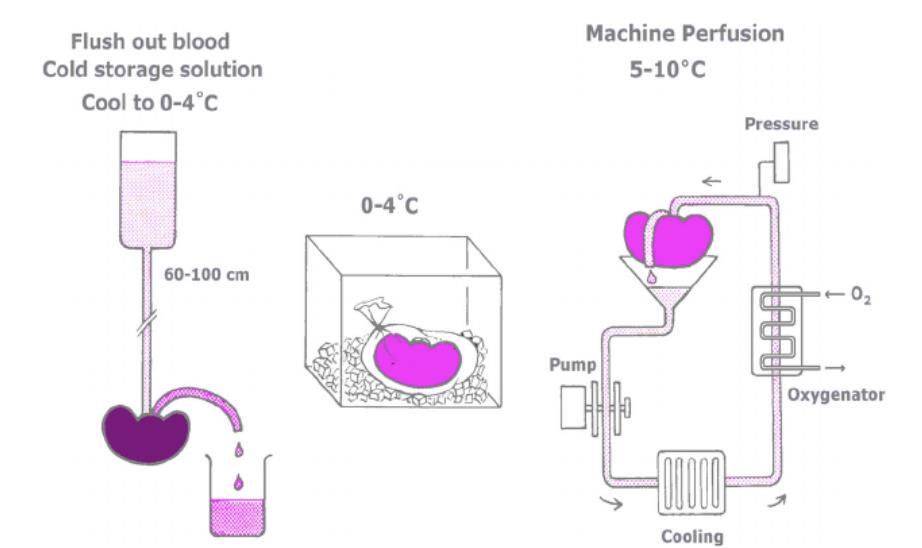
126
What is Heart in a Box and How does it work?
Heart in a box is a new technology that was developed in 2014 by Transmedics, an organ therapy transplant company. Heart in a box allows a donor heart to keep beating and functioning outside the body.
When Heart in a Box was developed, the discovery was made on how to transplant donor’s hearts that had stopped after death successfully. The Heart in a Box is composed of an organ specific perfusion machine with disposable and non-disposable parts and a compact wireless monitor.
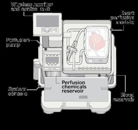
Image: Schematic representation of static cold storage and machine perfusion, 2014
The transplant process begins when the donor's heart is connected to a sterile circuit and once the heart is housed inside the portable device, the heart is reanimated, preserved with a unique fluid developed by the Victor Chang Cardiac Research Institute (Victor Chang Cardiac Research Institute 2022). The monitor that the heart is attached to, allows the cardiologist to see the heart is functioning properly by observing electrical activity that is always occurring in the heart, as the monitor displays a real-time system of organ measurements that include, aortic pressure, coronary flow, blood pressure and heart rate. The donor’s blood is warm (34°), oxygenated and is nutrient filled, which allows for an extended “out of body” time, and minimises the detrimental effects on the heart, such as tissue damage and the blood not receiving a substantial amount of oxygen, due to the deterioration of cells, if the blood were to be cold. The blood is then supplied and “is pumped through to the aorta, thereby passing blood through the coronary arteries, and deoxygenated blood perfuses through the left atrium through the coronary sinus and passes through the tricuspid valve to the right ventricle. The blood is then ejected through the pulmonary artery to the blood oxygenated and then finally is returned to the receiver” (Saez et al, 2014). Once the heart has been assessed and the cardiologist is satisfied, the heart is then transplanted into the recipient.
Advantages and Disadvantages of both Technologies
Heart in a Box is a new technology that has eliminated disadvantages from older heart transplant techniques, like the Static Cold Storage or has improved the disadvantages that the Static Cold Stage consists of. However, Heart in a Box still contains disadvantages compared to the Static Cold Stage.
127
Image: How does Heart in a Box work, Cleveland, 2012
Firstly, “OCS Heart is the only FDA approved technology for extracorporeal perfusion and preservation of Donor hearts in the U.S.” (Transmedics, 2022). Heart in a Box is the first commercially available system that allows the donor heart to be maintained in a warm perfused oxygenated state during the transfer period. As a result of this, Australia’s home of heart research, Victor Chang Cardiac Research Institution, says that Heart in a Box “reduces the amount of damage that can occur in the heart” and it “reduces the number of muscle cells that die” during the time that the heart is in the box (Victor Chang Cardiac Research Institute 2022). It reduces the amount of damaged that can occur in the heart, because the technique used is hyperthermic, meaning that the heart is consistently pumped with nutrient filled, warm blood (34°) throughout the transplant period, compared to the Static Cold Storage where the technique is hypothermic, meaning that the heart is resting at a cold temperature (4°), this increases the likelihood for tissue injury on the heart and muscles cells dying due to the lack of oxygen that the cells are receiving. Victor Chang Cardiac Research Institution also states that Heart in a Box is “making the heart more resilient to transplantation” and “improves heart function when it is restarted”, due to the heart still receiving oxygenated blood, allowing cellular respiration. Thus, minimising the amount of cell death that could potentially occur.
A major advantage that Heart in a Box has compared to the Static Cold Storage technique is it extends the amount of ischemic time - the amount of time the heart has outside the body. Transmedics Organ Care System (OCS), the founding company of Heart in a Box says that the heart can remain outside the body for up to “12 hours”, juxtaposed to the Static Cold Storage, where the heart can last for four hours. Director, UCLA Heart and Lung Transplants, Doctor Abbas Ardehali says, “OSC allows us to take the time variable out of the equation… A good illustration of this is, on an annual basis more than thirty or forty in Hawaii go unused because of the distance, these hearts cannot be transported to the mainland. This technology can potentially afford those hearts to the rest of the country” (Organ Care System OCS Heart, Transmedics, 2019).
Another significant advantage of Heart in a Box is the way the doctors can test the heart's condition before transplanting the heart into the recipient. The digital monitor allows the specialist to monitor the heart's aortic pressure, the rate in which it is beating, the blood pressure and the coronary flow as well as a live electrocardiogram (ecg). If the heart does begin to beat abnormally, the machine's setting can be adjusted to change the blood flow. This technology is positive because it optimises the chance of a successful heart transplant as doctors can see if the heart is functioning to a state where it can be transplanted, maximising the recipient's chance of survival. In an academic article by the University of Minnesota, evaluating Heart in a Box, Cardiovascular surgeon, Kenneth Laio says “This gives us time to assess the heart until about 10 minutes before we put it in…We will watch the heart work, pumping, until we are totally satisfied that the heart is usable” (Breining, 2017). Monitoring the heart has shown success for the patient’s post-surgery as seen through Dr Gero Tenderich “PROTECT 1 clinical trial” evaluating the “Safety and Performance of the Organ Care System for Heart Transplants”, the results show that “100% survival of patients 30 days post-surgery” and that “using the OSC allowed for patients

128
Image: Trandmedics, 2022
to spend less time on a ventilator and experience a quicker recovery in the hospital” (Science Daily, 2007). In contrast, a comparative study was demonstrated to evaluate heart transplant outcomes using Static Cold Storage technique, showing the mortality rate for the Static Cold Storage 30 days postsurgery was 13% out of the 24 participants (Sandro Spronga, et al, 2021). This survival rate could potentially reflect upon the fact that the Static Cold Storage does not allow doctors to assess the heart before it is transplanted into the recipient, which is a limitation to the recipient because there is a risk of fatality.
Transmedics are conducting an extended trial to “Evaluate the Organ Care System for use with unutilised donor hearts that may not meet current standard acceptance criteria for transplantation”, where 75 patients were enrolled (Transmedics, 2022). In this clinical trial, the target donors were “marginal donors” - people whose hearts might have been rejected by the traditional criteria for heart transplants. If this criterion is effective, more hearts will be available for transplants, therefore, less hearts will be wasted. The types of expanded criteria donor hearts used were:
● “Expected ischemic time >4 hours - 37%
● 20 or more mins of down time - 31%
● LVEF of 40-50% - 28%
● Older donors >55 years - 13%
● Coronary artery disease - 8%” (Transmedics, 2022)
The Static Cold Storage uses the traditional criteria for determining what a good heart looks like for transplantation. This includes:
● A donor who is younger than 55 years old
● A donor with no history of chest trauma or cardiac disease
● No history of low blood pressure or low oxygen in the blood
● A normal electrocardiogram and a normal echocardiogram
This expanded trial will be beneficial in determining whether “unuseful” hearts that fit in the traditional criteria can be used for possible transplants. The expanded trial will also limit the wastage of hearts that wouldn't have been acceptable in the traditional criteria that is used by the Static Cold Storage, because hearts will be acceptable in the new expanded criteria for the future.
However, Heart in a Box is quite costly for an individual, costing $250,000 USD. Thus, representing a barrier that could prevent many hospitals from acquiring the device and people not being able to afford the most substantial treatment they require. Juxtaposed to the Static Cold Storage, where the cost of standard care is from $70 to $205 USD, therefore making the Static Cold Storage significantly more accessible for hospitals to obtain this technique. As a result of Heart in a Box being a new technology, it is difficult to have access to the technology because it is very expensive and there is not a sustainable amount of data to prove the claims that have been made.
129
Table1 : Advantages and Disadvantages of ‘Heart in a Box’ and ‘Static Cold Storage’
Heart in a Box Static Cold Storage
Advantages
● FDA approved
● Heart is constantly beating outside the body - cellular respiration still occurs
● Heart is maintained in a warm perfused oxygenated state
● Reduces damage to the heart
● Hyperthermic technique
● Heart is still supplied with nutrients
● Ischemic time increased
● The heart can be monitored
● The expanded trial
Disadvantages
● Expensive
● Difficult to access
● Limited amount of scientific data
● Less expensive
● More accessible to hospitals
● Extensive amount of scientific data
● Hypothermic technique (heart is kept cold) - no cellular respiration
● Increased damaged to the heart
● Limited amount of ischemic time
● The heat cannot be monitored
● Heart is not beating
● Heart is not supplied with nutrients
● Traditional criteria only
Evaluation of both technologies
As hypothesised, it is evidently clear that ‘Heart in a Box’ is a technology that is significantly effective as a strategy for heart transplants, which is in need because of the high prevalence of heart disease globally. ‘Heart in a Box’ is a superior technology rather than the ‘Static Cold Storage’ as it is the first commercially available system that allows the donor heart to be maintained in a warm perfused oxygenated state during the transfer period, the heart is constantly beating outside the body, allowing cellular respiration to occur, the heart is maintained in a warm perfused state at 34° and is still provided with the necessary nutrients and oxygen, thus decreasing the risk of damaging the heart. Heart in a Box also increases and extends the ischemic time, allowing the heart to be out of the body for up to 12 hours, unlike the Static Cold Storage technique which has an ischemic time of 4 hours. The expanded trial that Transmedics is conducting is also great for the future of heart transplants as it includes ‘marginal donors’, meaning that there will be a decreased amount of wastage and it is providing more people with hearts. But, considering that Heart in a Box is a new technology, it is difficult for hospitals and individuals to access the technology because it is exceptionally expensive and there is little scientific data to gain greater knowledge about how to improve the technology, contrasting the Static Cold Storage technique where it is significantly less expensive to both hospitals and individuals and easily more accessible. To conclude, ‘Heart in a box’, is extremely more effective compared to the ‘Static Cold Storage’ against heart disease.
130
References
Akhtar, M 2014, Schematic representation of static cold storage and machine perfusion, Photograph, N.a., viewed 8 May 2022, <https://www.researchgate.net/figure/Schematic-representation-of-staticcold-storage-and-machine-perfusion-Left-before_fig2_275257408>.
Eisen, H 2021, Patient education: Heart transplantation (Beyond the Basics), viewed 8 May 2022, <https://www.uptodate.com/contents/heart-transplantation-beyond-thebasics#:~:text=More%20than%205000%20cardiac%20 transplants,should%20receive%20a%20heart%20transplant.>.
Faris, D 2017, ‘Heart in a Box’ a Big Step Forward for Organ Transplants, ZME Science, viewed 8 May 2022, <https://www.zmescience.com/medicine/heart-in-a-box-a-big-step-forward-for-organtransplants/>.
Greg Breining, G 2017, HEART IN A BOX, N.a., viewed 8 May 2022, <https://med.umn.edu/newsevents/medical-bulletin/heart-box>.
Heart Transplant 2022, John Hopkins Medicine, viewed 8 May 2022, <https://www.hopkinsmedicine.org/health/treatment-tests-and-therapies/heart-transplant>.
Increasing Survival Of Organ Transplant Patients By Reducing Time Interval For Transported Organs 2007, Science Daily, viewed 8 May 2022, <https://www.sciencedaily.com/releases/2007/04/070426144823.htm>.
Jing, L, Yao, L & Zhao, M 2018, Organ preservation: from the past to the future, pdf, viewed 8 May 2022, <https://www.nature.com/articles/aps2017182.pdf?origin=epub>.
Nilsson, J 2021, Non-ischaemic Heart Preservation Versus Standard Cold Storage in Human Heart Transplantation (NIHP2), U.S National Library of Medicine, viewed 8 May 2022, <https://clinicaltrials.gov/ct2/show/NCT04066127>.
OCS Heart 2022, Transmedics, viewed 8 May 2022, <https://www.transmedics.com/ocs-hcp-heart/>.
Saez, D, Zych, B & Sabashnikov, A 2014, Evaluation of the Organ Care System in Heart Transplantation With an Adverse Donor/Recipient Profile, pdf, viewed 8 May 2022, <https://www.annalsthoracicsurgery.org/article/S0003-4975(14)01499-4/pdf>.
Sponga, S, Benedetti, G & Manna, N 2021, Heart transplant outcomes in patients with mechanical circulatory support: cold storage versus normothermic perfusion organ preservation, viewed 8 May 2022, <https://pubmed.ncbi.nlm.nih.gov/33221874/>.
Transplant success with heart-in-a-box method 2020, viewed 8 May 2022, <https://www.hospitalhealth.com.au/content/clinical-services/news/transplant-success-withheart-in-a-box-method-454317287>.
Victor Chang Cardiac Research Institute 2022, Heart in a Box, viewed 26 April 2022, <https://www.victorchang.edu.au/heart-in-a-box>.
131
Victor Chang Cardiac Research Institute 2022, Heart Transplant Research Breakthrough, N.a., Sydney, viewed 8 May 2022, <https://www.victorchang.edu.au/news/heart-transplant-breakthrough>.
World Health Organisation 2020, The top 10 causes of death, Australian Government, viewed 8 May 2022, <https://www.who.int/news-room/fact-sheets/detail/the-top-10-causes-of-death>.
Wong, Y, Law, J & Sharma, V 2021, Real World Experience with Transmedics Organ Care System in Cardiac Transplantation with Donor Organs Associated with Marginal Risk Factors, The Journal of Heart and Lung Transplants, viewed 8 May 2022, <https://www.jhltonline.org/article/S10532498(21)00583-0/fulltext>.
132
Evaluating the Appropriateness of Early Detection/Treatment and Prevention Initiatives for Cancers in NSW
Hasnain Aly (Year 12)
The Illawarra Grammar School, 10/12 Western Avenue, Wollongong, NSW, Australia, 2500
What Is Cancer?
Cancers are a group of diseases characterised by abnormal and uncontrolled cell division which results in the development of tumours (WHO 2019). Cancerous, or malignant, tumours are tumours that spread to other parts of the body, usually nearby tissue, but can spread through the cardiovascular or lymphatic systems, reaching distant regions in a process known as metastasis. Cancers are categorised by the area within which they develop. For example, kidney cancers are one of the most likely to metastasise, commonly spreading to the liver or lung (NCI 2020). These secondary cancers still consist of cancerous kidney cells, not liver or lung cells.
WhatCausesCancer?
Cancers are caused by genetic mutations affecting the process of cell division. These mutations result in cells reproducing without being signalled to, or cells incorrectly receiving signals to cease division and/or undergo apoptosis (NCI 2020). Genetic mutations may arise at random, from genetic damage due to exposure to carcinogenic substances, or are inherited. Approximately 5% of cancers are inherited, the rest being sporadic (NCI 2018).
RiskFactorsForCancers
Age is a significant risk factor for developing cancer that cannot be avoided. The probabilityof cancerous mutations occurring increases over time . Other risk factors include chronic illnesses, lifestyle choices such as smoking and alcohol, infection with certain viruses, e.g. Human Papilloma Virus or Epstein Barr Virus, or hormonal factors such as increased oestrogen levels, which all impact particular age groups. In order to minimise the health and economic costs of cancer, early detection, treatment and prevention are all important paths of action (Drexler, 2019). In order to efficiently target these approaches, resources for particular cancers should be directed at the age groups where they will have the greatest impact. These may include targeted measures such as preemptive screening programmes, early interventions and educational campaigns.
ResearchAimandQuestions
As a result of the background research conducted in this study, it has been demonstrated that age is a significant risk factor in the development of cancers, and as it cannot be controlled, its unavoidable influence on the prevalence of cancer should be strategically combatted.
ResearchAim
This study aims to evaluate the suitability of early screening, treatment and prevention measures for three different types of cancers through examining trends in prevalence in types across age groups. To achieve this, trends in prevalence of three specific cancers across age groups will be identified and compared to current cancer initiatives in order to evaluate them.
ResearchQuestions
133
What are trends in prevalence of three types of cancers across different age groups?
Do these trends support existing early detection, treatment and prevention programs?
WhyIsEarlyDetection/TreatmentandPreventionImportant?
With advances in modern medicine, the prevalence of infectious diseases in developed nations has significantly reduced, leaving non-infectious diseases to place a significant burden on the healthcare systems of such nations. It is widely accepted that early detection, treatment and prevention of any disease is extremely beneficial both for patients and the healthcare system. Not only does it carry economic benefits, but it also reduces the physical and psychological discomfort for patients and their carers (NIB, 2021). These benefits are extremely relevant in relation to cancers, due to the significant reduction in cure rates and increased treatment required if cancers are not detected or treated early in their development (Drexler, 2019).
RisksofPreemptiveScreening
While pre-emptive screening may be beneficial for the early detection of cancer, there is also the risk of overdiagnosis and overtreatment, which varies between different cancers. Overdiagnosis occurs when screening detects an abnormality that would not actually cause a problem for the patient, for example non-malignant breast masses. Overtreatment occurs when a cancer is unnecessarily treated, resulting in treatment toxicity and unnecessary medical costs. Both overdiagnosis and over screening can cause significant psychological and physical consequences, as well as placing unnecessary burden on medical providers.
An example of this problem is in the case of prostate cancer screening. Basch et al, in their extensive 2012 study recommended that PSA screening for prostate cancer be discouraged for men with a life expectancy less than ten years as harms outweigh potential benefits. The specific harms include complications from unnecessary biopsy and treatment (surgery or radiotherapy).
These recommendations were made on the basis of evidence from five large randomized clinical trials, which was then evaluated by a panel of clinical experts and published in a leading peer-reviewed journal, making their findings extremely reliable and valid. Basch et al’s paper strongly recommended that patients to be provided with sufficient information to provide informed consent for PSA screening. Information should be available in simplified language for patients. Gøtzsche and Nielsen’s 2006 study on the risks and benefits of mammography screening for breast cancer went as far as to provide such an information sheet within the paper for clinical use.
StudyMethodology DataSource/Collection
Data for this study has been sourced from The Australian Institute of Health and Welfare (AIHW) Cancer Data in Australia 2021: Book 1a – Cancer incidence (age-standardised rates and 5-year age groups). This source of data is highly valid and reliable as it originates from a government organisation, and contains an extensive breadth of data spanning almost 40 years.
134
ChosenCancers
Research was conducted into cancers with established screening programs within Australia. Three cancers (breast, cervical and prostate) were selected due to their applicability to the research question and the researcher’s personal interest. Both breast and cervical cancers are the targets of extensive early detection and prevention programs within Australia, allowing their analysis to yield insightful results. Additionally, analysing data on prostate cancer will provide an interesting perspective for a cancer where the benefits of screening are controversial and highly debated within the medical comunity.
DataAnalysisMethod
Data was available for five year age groups up to 90+, and all ages combined. Data was provided from 1982-2021, but data from 2018-2021 is expected prevalence rather than observed. Due to this, the five most recent years with observed data (2013-2017) were used for data analysis. The means of each age group’s age specific incidence rates across the five years were calculated and plotted in a frequency histogram. The mean was used as the chosen method of centrality due to the unskewed nature of the data set.
HypothesisandExpectedOutcomes Hypothesis
Data analysed will strongly support existing initiatives for early screening/treatment and prevention as the data source is highly reliable, and Australia is a highly developed country with extensive healthcare systems.
NullHypothesis
Data analysed will not support existing initiatives for early screening/treatment and prevention. If the null hypothesis is accepted by analysis of data in this study, this would indicate errors in study methodology, as initiatives for early screening/treatment and prevention are backed up by extensive professional data analysis and research.
CriteriatobeEvaluatedAgainst
The appropriateness of initiatives for early detection/treatment and prevention will be evaluated for how well they align with the data analysed. The ages of highest incidence of the chosen cancers will be compared to the ages where screening or prevention initiatives are targeted, which will be used to a judge their appropriateness. Additionally, current scientific knowledge will be considered when evaluating initiatives to consolidate analysis of data.
Findings
Raw data tables for the three chosen cancers are available in appendices.
General
A significant finding yielded in this study is that the incidence rates of all cancers have followed a consistent trend of increase over the past 40 years, even when adjusted for population (figure 1). As this is not the focus of this study, it will not be investigated further, but could be a focus for future research.
135
When analysing incidence rates for the three chosen cancers, it was found that that cervical cancer has a significantly lower incidence compared to the other two cancers (figure 2).
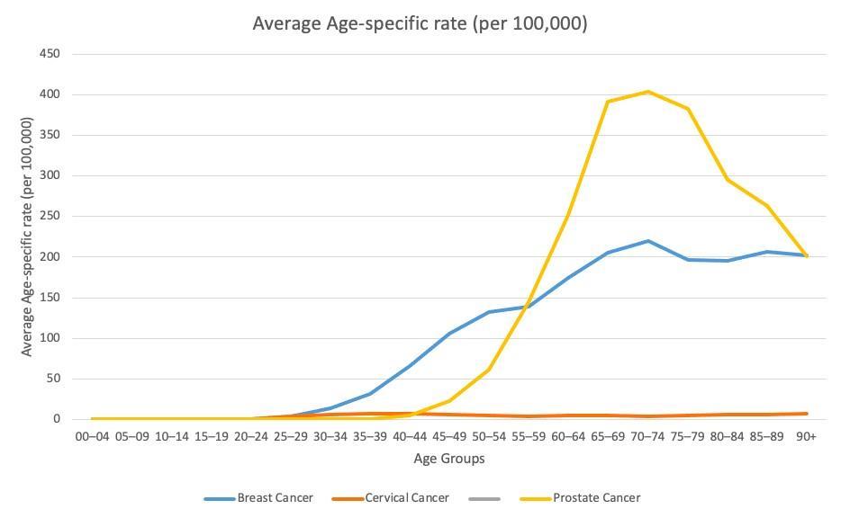
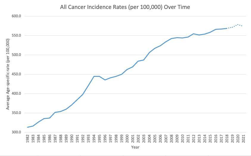
136
Figure 1: Incidence rates for all cancers 1982-2021, adjusted for population. Note that dotted line represents projected data.
Figure 2: Age specific incidence rates for chosen cancers 2013-2017.
Also demonstrated in figure 2, both breast and prostate cancer peak in incidence between 70-74 years (although prostate cancer is around double that of breast cancer), compared to the average peak for all cancers at 85-89 years (figure 3). Cervical cancer peaks in incidence at an even younger age 35-39 (figure 2.5).
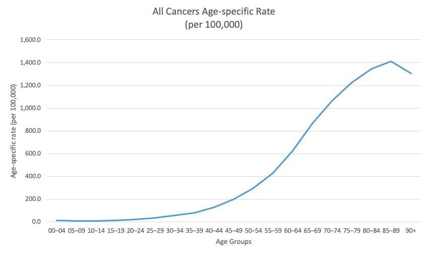
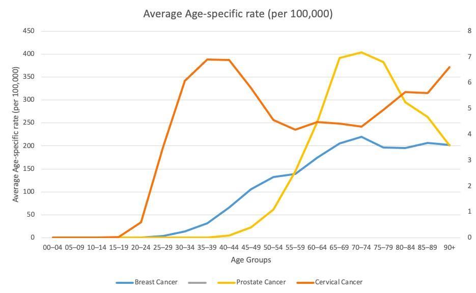
137
Figure 2.5: Age specific incidence rates for chosen cancers 2013-2017 with cervical cancer graphed on secondary axis.
Figure 3: Age specific incidence rates for all cancers 2013-2017.
Figure 4: Age specific incidence rates for breast cancer 2013-2017.
The Australian Cancer Council, Australia’s leading cancer charity, recommends screening mammography to be conducted every two years from ages 50-75.
Additionally, the American College of Obstetricians and Gynaecologists, America’s leading group of medical professionals specialising in women’s health, recommends that mammography screening should take place every one to two years starting from age 40, no later than age 50. They also recommend that screening continue until at least age 75.
This advice from two major authorities in the field of breast cancer is heavily supported by the analysis of data, which shows a strong increase in incidence around ages 45-49, which continues to increase until ages 70-74, before plateauing (figure 4).
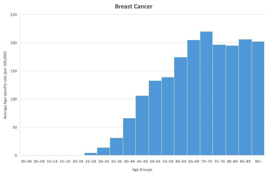
In Australia, free mammography screenings are available for women aged 40 and over, and letters of invitation are sent every two years to women aged 50-75. This initiative strongly aligns with the trends seen in figure 4. Furthermore, stopping screening invitations at age 75 is highly supported by current scientific knowledge, with a 2011 paper from Ellen Warner published in the New England Journal of Medicine estimating that only two deaths per 1,000 would be prevented by screening women of the age of 70 to 74 years, and little to no evidence suggesting benefits of screening beyond the age of 74. This evidence strongly supports Australia’s early detection and treatment program.
However, mammography screening for breast cancer carries risk of overdiagnosis and overtreatment, and while it does carry benefits, the level of benefit is unclear (Gøtzsche & Nielsen, 2006). It was estimated by Gøtzsche and Nielsen that mammography screening for breast cancer reduces mortality by 15%, but causes 30% overdiagnosis, and that 10% of women who have mammography screening for breast cancer will suffer psychological distress due to false positives. Based on this study, and other previously discussed studies on the risks of overdiagnosis, it is strongly recommended that women receiving mammography screening are fully informed of its risks and benefits. The researcher would like
138 BreastCancer
to direct readers to Gøtzsche and Nielsen’s information sheet in their paper for more information and advise that women be provided with such a resource when offered mammography screenings.
Figure 5: Age specific incidence rates for cervical cancer 2013-2017.
The World Health Organisation (WHO) advises that over 95% of cervical cancers are caused by the human papillomavirus (HPV), which is sexually transmitted and affects the majority of sexually active individuals, with about 90% of cases clearing up spontaneously. Furthermore, cervical cancers take around 15-20 years to develop in otherwise healthy women. This information aligns with the analysis of data, as incidence begins to increase at around 20-24, spiking significantly from 30-49. This indicates that women who became infected with HPV in their youth while they were sexually active will only show symptoms of cervical cancer around 15-20 years down the line. In order to prevent HPV related cervical cancer, the Australian government introduced a school based HPV vaccination program for females aged 12-13, which was modified to include males in 2017. Additionally, Australia offers free cervical cancer screenings for women aged 25-75 every five years. Australia as a country has been at the forefront of the fight against HPV and cervical cancer since the 1970s (Stenhouse, 2016), and it was only in 2020 that the World Health Assembly adopted a global strategy to eliminate cervical cancer. This strategy consists of a three staged prevention, including HPV vaccination for girls aged 9-14, and screening for women aged 30 and over. This approach has proven to be highly successful, with a highly reliable 2007 epidemiological study from Kevin A Ault finding that administering HPV vaccine in women “could substantially reduce the incidence of HPV16/18-related cervical precancers and cervical cancer”. Not only did this study consist of a large sample size (n=20,583), but it was also randomised, controlled (with a placebo group), and double blind. The appropriate methodology results in the conclusions of this study to be considered extremely valid and reliable.
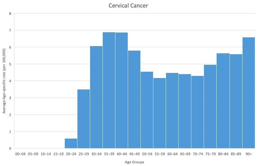
139
CervicalCancer
Australia’s initiatives for combating cervical cancer through early detection and prevention (HPV vaccine) are supported by the analysis of data in this study, as well as current scientific knowledge.
ProstateCancer
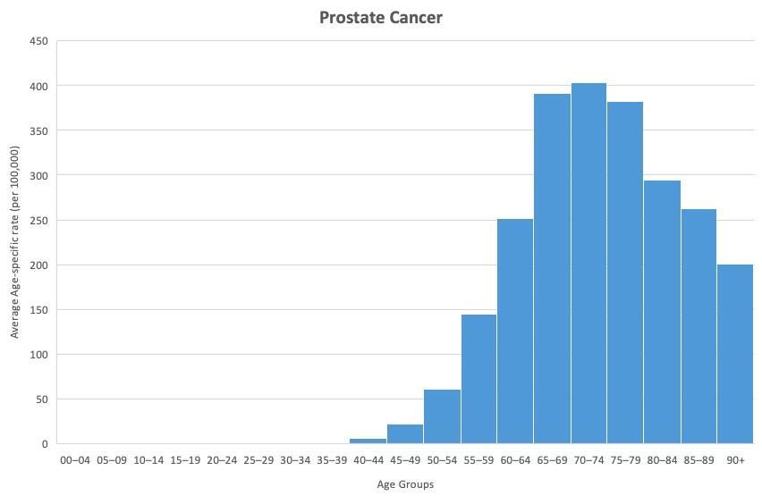
The Prostate Cancer Foundation of Australia (PCFA) statesthat approximately 50% of males will have some form of prostate disease before age 70. Australia has one of the highest incidence of prostate cancer rates globally, with one in seven Australian men being diagnosed with prostate cancer during their lifetimes. Furthermore, it is also the second most diagnosed cancer and the third most fatal cancer in Australian men (Cancer Council Australia, 2020). This is supported by analysis of data, where the incidence rate of prostate cancer was significantly higher than other cancers, including breast cancer
Prostate cancer has been the recipient of significant misconception surrounding early detection screening, possibly due to the invasive nature of the digital rectal examination (DRE), which is no longer recommended for routine screening as it only helps detect tumours near the rectum. The prostate specific antigen (PSA) blood test is generally employed to test for an antigen produced by the prostate gland, higher levels of which may indicate some form of prostate disease (Prostate Cancer Foundation of Australia 2021). However, PSA testing is problematic as it does not definitively test for prostate cancer, and may present false positives due to other prostate diseases. It can also overdiagnose low-risk prostate cancers, resulting in unnecessary treatments with potential harmful side effects and psychological distress for patients and their family (Basch et al., 2012).
Due to these potential risks, guidelines recommend that PSA testing is appropriate for men aged 40/4569 with a family history, and ages 50-69 without family history. Additionally, screening over the age of 70 carries a significantly increased risk of overdiagnosis and overtreatment. This advice aligns with the analysis of data as incidence begins to rise throughout 50s
140
Figure 6: Age specific incidence rates for prostate cancer 2013-2017.
Conclusion
This study aimed to evaluate the suitability of early screening, treatment and prevention measures for three different types of cancers through the examination of trends in prevalence in cancer types across age groups and consolidating with current scientific knowledge. Throughout this report, a comprehensive evaluation has demonstrated the high suitability of Australia’s early screening, treatment and prevention measures for three selected cancers, resulting in the acceptance of the hypothesis.
Bibliography
A Pray, L 2008, Errors in DNA Replication | Learn Science at Scitable, Nature.com, Nature Education, viewed 28 March 2022,
<https://www.nature.com/scitable/topicpage/dna-replication-and-causes-of-mutation409/#:~:text=Nonetheless%2C%20these%20enzy mes%20do%20make,every%20time%20a%20cell%20divides!>.
ACOG 2017, Mammography and Other Screening Tests for Breast Problems, Acog.org, viewed 7 April 2022, <https://www.acog.org/womens-health/faqs/mammography-and-other-screening-tests-for-breastproblems>.
ACRF 2021, Types of Cancer | What Are The Different Types of Cancer | ACRF, ACRF, viewed 25 March 2022,
<https://www.acrf.com.au/support-cancer-research/types-ofcancer/?gclid=CjwKCAjwrfCRBhAXEiwAnkmKmR_IlLgFuXcqdUUvknw8Z6 tRfISyCEpCZ8CCXVIjND1Laz_SovjgRoCMBIQAvD_BwE&fwp_load_more=2>.
AIHW 2020, How healthy are Australians? - Australian Institute of Health and Welfare, Australian Institute of Health and Welfare, viewed 4 May 2022, <https://www.aihw.gov.au/reports/australiashealth/how-healthy-are-australians>.
AIHW 2021, Cancer data in Australia, Cancer incidence by age visualisation - Australian Institute of Health and Welfare, Australian Institute of Health and Welfare, viewed 25 March 2022, <https://www.aihw.gov.au/reports/cancer/cancer-data-in-australia/contents/cancer-incidence-by-agevisualisation>.
Ault, KA 2007, ‘Effect of prophylactic human papillomavirus L1 virus-like-particle vaccine on risk of cervical intraepithelial neoplasia grade 2, grade 3, and adenocarcinoma in situ: a combined analysis of four randomised clinical trials’, The Lancet, vol. 369, no. 9576, pp.
1861
1868, viewed 6 May 2022, <https://pubmed.ncbi.nlm.nih.gov/17544766/>.
Autier, P & Boniol, M 2018, ‘Mammography screening: a Major Issue in Medicine’, European Journal of Cancer, vol. 90, pp. 34–62, viewed 4 May 2022, <https://pubmed.ncbi.nlm.nih.gov/29272783/>.
Basch, E, Oliver, TK, Vickers, A, Thompson, I, Kantoff, P, Parnes, H, Loblaw, DA, Roth, B, Williams, J & Nam, RK 2012, ‘Screening for Prostate
Cancer With Prostate-Specific Antigen Testing: American Society of Clinical Oncology Provisional Clinical Opinion’, Journal of Clinical Oncology, vol. 30, no. 24, pp. 3020–3025, viewed 6 May 2022, <https://pubmed.ncbi.nlm.nih.gov/22802323/>.
Beard, J 2019, Info, PSA Testing, viewed 27 April 2022, <http://psatesting.org.au/info/>.
Cancer Council Australia 2017, Early detection and screening, Cancer.org.au, viewed 25 April 2022, <https://www.cancer.org.au/cancer-information/causes-and-prevention/early-detection-andscreening>.
Cancer Council Australia 2020, Mammogram, Cancer.org.au, viewed 7 April 2022, <https://www.cancer.org.au/mammogram>.
Cancer Council Australia 2022, Early detection of prostate cancer, Cancer.org.au, viewed 25 April 2022, <https://www.cancer.org.au/cancer-information/causes-and-prevention/early-detection-andscreening/early-detection-of-prostate-canc er>.
141
–
Drexler, M 2019, The Cancer Miracle Isn’t a Cure. It’s Prevention., Harvard Public Health Magazine, Harvard Public Health Magazine, viewed 31 March 2022,
<https://www.hsph.harvard.edu/magazine/magazine_article/the-cancer-miracle-isnt-a-cure-itsprevention/>.
Gøtzsche, PC & Nielsen, M 2006, ‘Screening for breast cancer with mammography’, in PC Gøtzsche (ed.), Cochrane Database of Systematic Reviews, viewed 6 May 2022, <https://pubmed.ncbi.nlm.nih.gov/17054145/>.
Australian Government Department of Health 2019a, BreastScreen Australia Program, Australian Government Department of Health, viewed 25 April 2022,
<https://www.health.gov.au/initiatives-and-programs/breastscreen-australia-program>.
Australian Government Department of Health 2019b, National Cervical Screening Program, Australian Government Department of Health, viewed 25 April 2022,
<https://www.health.gov.au/initiatives-and-programs/national-cervical-screening-program>.
http://canceraustralia.gov.au 2020, HPV immunisation, National Cancer Control Indicators, viewed 27 April 2022,
<https://ncci.canceraustralia.gov.au/screening-and-immunisation/immunisation/hpvimmunisation#:~:text=In%202007%2C%20the%20s chool%2Dbased,include%20male%20students%20in%202013.>.
http://www.canceraustralia.gov.au 2019, Health professionals | Cancer Australia, Canceraustralia.gov.au, viewed 28 April 2022, <https://www.canceraustralia.gov.au/cancer-types/prostatecancer/clinicians-hub>.
Mühlhauser, I 2007, ‘Ist Vorbeugen besser als Heilen?’, Zeitschrift für ärztliche Fortbildung und Qualität im Gesundheitswesen - German Journal for Quality in Health Care, vol. 101, no. 5, pp. 293.e1–293.e9, viewed 4 May 2022, <https://pubmed.ncbi.nlm.nih.gov/17711254/>.
National Cancer Institute 2020, Metastatic Cancer: When Cancer Spreads, National Cancer Institute, Cancer.gov, viewed 25 March 2022, <https://www.cancer.gov/types/metastatic-cancer>.
NCI 2015, Risk Factors for Cancer, National Cancer Institute, Cancer.gov, viewed 28 March 2022, <https://www.cancer.gov/about-cancer/causes-prevention/risk>.
NCI 2022, Dictionary of Cancer Terms, National Cancer Institute, Cancer.gov, viewed 25 March 2022, <https://www.cancer.gov/publications/dictionaries/cancer-terms/def/cancer>.
NCI 2020, Annual Immunisation Coverage Report 2020 available now | NCIRS, Ncirs.org.au, viewed 27 April 2022, <https://www.ncirs.org.au/annual-immunisation-coverage-report-2020-availablenow>.
NHMRC 2014, PSA Testing for Prostate Cancer in Asymptomatic Men Information for Health Practitioners, NHMRC, March, viewed 8 May 2022, <https://www.nhmrc.gov.au/sites/default/files/documents/reports/clinical%20guidelines/m en4d-psa-testing-asymptomatic.pdf>.
NIB 2021, Why is prevention better than cure?, Nib.com.au, nib, viewed 4 May 2022, <https://www.nib.com.au/the-checkup/prevention-is-better-than-cure>.
NCI 2021, What Is Cancer?, National Cancer Institute, Cancer.gov, viewed 25 March 2022, <https://www.cancer.gov/about-cancer/understanding/what-is-cancer>.
Prostate Cancer Foundation of Australia 2021a, Prostate cancer – a guide for newly-diagnosed men, Issuu, viewed 27 April 2022, <https://issuu.com/prostatecancerfoundationaus/docs/pcf13457__prostate_cancer_-_a_guide_for_newly_dia>.
Prostate Cancer Foundation of Australia 2021b, What you need to know about prostate cancer, Issuu, viewed 27 April 2022, <https://issuu.com/prostatecancerfoundationaus/docs/pcf13452__what_you_need_to_know_about_prostate_ca>.
Stenhouse, A 2016, How Australians have been leading the fight against cervical cancer since 1978 | Know Pathology Know Healthcare, Know Pathology Know Healthcare | The engine room of healthcare explained, viewed 27 April 2022, <https://knowpathology.com.au/australians-leading-cervical-cancer-fight/>.
142
Warner, E 2011, ‘Breast-Cancer Screening’, New England Journal of Medicine, vol. 365, no. 11, pp. 1025
1032, viewed 6 May 2022, <https://pubmed.ncbi.nlm.nih.gov/21916640/>. WHO 2019, Cancer, Who.int, World Health Organization, viewed 25 March 2022, <https://www.who.int/health-topics/cancer>.
143
–
Asthma and an evaluation of the effectiveness of short acting bronchodilators as a method of treatment
Liam Harvey (Year 12)
The Illawarra Grammar School, 10/12 Western Avenue, Wollongong, NSW, Australia, 2500
Introduction
According to the World Health Organisation (WHO) – a specialised agency responsible for monitoring and managing international public health, 262 million people in 2019 were impacted by bronchial asthma and its symptoms, resulting in over 460000 deaths globally. The most common treatment method for bronchial asthma is the use of an inhaled short-acting bronchodilator.

In a changing world where technology is advancing, new industries and power solutions are producing more air pollutants than ever before. 95% of the world’s population experiences exposure to air particulates and pollutants that are above the WHO’s recommended guidelines of 10µg/m3 (Ritchie & Roser 2022). This constant and increasing exposure to unsafe concentrations of air pollutants and particulates is a factor that exacerbates the symptoms of asthma on those with the chronic condition, leading to more frequent application of treatment solutions (Asthma Australia, 2021).
Due to this global increase in the air pollutant level into unsafe quantities that could be a trigger factor and impact those with asthma, an evaluation of the effectiveness of short acting bronchodilators is necessary to ensure their viability for the future.
ResearchQuestion+SubQuestions
The main, guiding research question for this evaluation is: Are short acting bronchodilators an effective treatment for bronchial asthma?
To answer this main question, a range of sub-questions need to be addressed:
• What is bronchial asthma?
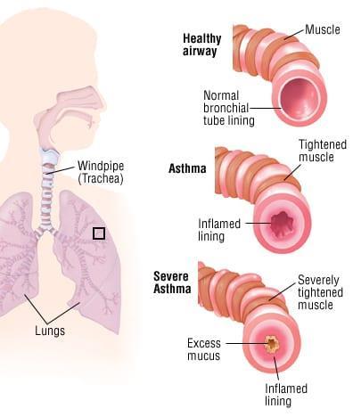
• What are short-acting bronchodilators?
• What are the measures of effectiveness of bronchodilators?
• What are the technologies that can boost their effectiveness?
Asthma
According to the Global Initiative for Asthma (GINA): an international organisation that coordinates asthma control programs, research, and guidelines, and Asthma Australia: An Australian organisation that aims to assist and educate those with asthma, asthma is defined as a chronic noncommunicable disorder where common, characterising symptoms include:
• airway inflammation
• constriction of airway muscles
• bronchial hyperresponsiveness
• wheezing
• persistent cough
• chest tightness
• shortness of breath
• excessive mucus production
144
Diagram 2: Diagram of the differences in a normal airway, an asthmatic airway, and a severely asthmatic
Symptoms of asthma can vary in duration and intensity, making diagnosis reliant on a case-by-case understanding and historical basis. More intense and severe symptoms can result in hospitalisations and death, as the person is unable to breathe. There are a range of common factors and triggers that can cause an episodic flare-up of asthma symptoms that can divide asthma into a range of factor phenotypes, including but not limited to (Asthma Australia 2021):
Phenotype Cause
Allergic Asthma
Allergens including pollen, dust, and animal dander.
Non-allergic Asthma Includes viruses (cold/flu), smoke and aerosol sprays (deodorants).
Occupational Asthma
Exercise-induced Asthma
Nocturnal Asthma
Occupational triggers such as chemicals, fumes, and coal dust.
Caused by exertion and physical activities
Factors related to the night, such as dust mites and weather conditions
Specifically, regarding the pathophysiology of asthma and the body’s response to these factors, specific antibodies called Immunoglobulin E (IgE) are released due to the detection of one of these factors present in the environment or in the body. The IgE antibodies bind to mast cells, which are immune cells that control the release of inflammatory chemicals such as histamine, and causes them to release those chemicals, generating the symptoms of bronchoconstriction and inflammation, as they increase blood flow to the airways and cause the smooth muscle cells of the airway to contract (See Diagram 1) (Sinyor, B & Perez, LC 2021).
According to the Australian Institute of Health and Welfare (AIHW) website – a government-run institute that provides meaningful information and statistics regarding health and welfare, 11% of the Australian population (2.7 million people) have asthma, as collected from 2017-2018. This means that 11% of the population is using some form of inhaled short-term bronchodilator to combat their symptoms of asthma, supporting the need for an evaluation of short-term bronchodilator effectiveness.
145
Inhalers


Short-acting bronchodilators, also known as asthma relievers, are medication that is fast-acting to quickly counteract the symptoms of asthma when they are exacerbated. Specifically, they relax the smooth muscle cells within the airway which contract when trigger factors occur in the environment. The most common bronchodilator chemical used in Australia is called salbutamol, and there are four main relievers that use this chemical: Ventolin, Asmol, Zempreon and Airomir (See Diagram 2) (Asthma Australia, 2021). These relieving inhalers are not to be confused with preventers, which are used every day to provide a baseline level of protection from symptoms. They are commonly composed of an aluminium canister with a blue/grey plastic housing (Asthma Australia, 2021). Chemically, relievers operate by dispersing the bronchodilator (in the case of the Diagram 2, salbutamol) as an aerosol – a gas with fine particles of the medicine dispersed inside of it. This will provide quicker access to the airways and the bloodstream, which is where the salbutamol can take effect. This means that the medication will work within minutes, maximising relief from symptoms and preventing further exacerbation. Salbutamol, also known as a beta-2 agonist, works by activating the beta-2 receptor. This receptor is present in a range of cell groups, including cardiac cells and smooth muscle cells – when activated in smooth muscle cells, it causes them to relax, and when activated in cardiac cells, leads to an overall increase in heart rate, according to research conducted by researchers from the Alexandria School of Medicine, and the University of Florida (Abosamak, N & Shahin, M 2021).
Because of this, a potential side effect of the use of salbutamol is an increase in heart rate, as the chemical cannot target specific cells – hence it may activate beta2 receptors in cardiac cells (Syed, SA, et al. 2021).
Potential additions to current reliever technology include a powdered bronchodilator that is easier to use for those with inhibited use of aerosol relievers, called terbutaline (Figure 3), and spacer technology that increases the amount of bronchodilator that reaches and is absorbed into the airways (Figure 4).


146
Diagram 3: Image of the 4 most common inhalers in Australia, all of which use salbutamol (Asthma Inhalers used in Australia, 2021)
Diagram 3: Image of a dry powder reliever that uses terbutaline (Asthma Inhalers used in Australia 2021)
Diagram 4: Image of a plastic spacer used to improve bronchodilator distribution in the airways (Spacer, 2021)
Prediction
Based on the background research conducted, it is predicted that inhaled short-acting bronchodilators are an effective method of treating bronchial asthma with minimal side-effects. Furthermore, it is predicted that technologies such as spacers can improve the effectiveness of inhaled short-acting bronchodilators delivered using current reliever technology.
Effectivenessofreliever’sintreating Asthma
The effectiveness of short-acting bronchodilator relievers will be measured using the following criteria:
• Long-term impact on asthmarelated hospitalisations since introduction of short-acting bronchodilators
• Impact on variable lung function tests conducted through spirometry
• Cost
A study conducted in Salvador City, Brazil by C. Souza-Machado, A, et al – a group of Brazilian researchers, found that there was an inverse relationship between the introduction of inhaled short-acting bronchodilator relievers as a method of asthma treatment and hence the number of asthmatic patients using inhaled short-acting bronchodilator relievers, and the hospitalisation rate per 10000 people. The study analysed data before and after the implementation of the ProAR program in the city, which dispensed 220889 units of inhaled reliever medication to those in need. The middle line of Figure 1 represents an 87.5% decrease in the hospitalisation rate of asthmatic patients in Salvador between 2002-2006. Figure 2 further illustrates the impact of relievers on the hospitalisation rate, with a drop from approximately 0.09% of asthmatic patients going to hospital in 2003, to approximately 0.02% in 2006.

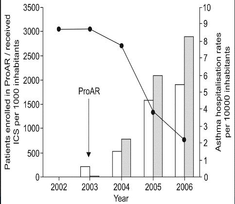

Within Australia, according to the Australian Institute of Health and Welfare, there were 38792 hospitalisations in 2017-18 where the primary cause was asthma-related symptoms. According to Asthma Australia, the National Service Improvement Framework for Asthma was released in 2005 and was a significant step in improving the accessibility of and the quality of short-acting bronchodilator medication in Australia. Figure 3 shows the overall decrease in hospitalisations for both groups aged 014, and the fluctuations in hospitalisations for both groups aged 15+. It can be inferred that this decrease in hospitalisations was contributed to by this Framework, and hence the use of short-acting
147
Figure 1: Graph showing the impact of the ProAR dispensing program on the asthmatic hospitalisation rate in Salvador City. Asthmatic inhabitants are represented by the middle line, and the program was implemented in 2003 (represented by the arrow) (Souza-Machado, C, et al., 2009)
Figure 2: Combination graph highlighting the inverse relationship between the number of patients enrolled in the ProAR dispensing program and the asthma hospitalisation rates per 10000) (Souza-
bronchodilators to combat the exacerbated symptoms of asthma. A decrease in hospitalisations correlates to an increase in the use of relievers to combat exacerbated symptoms. Spirometry is a method of assessing the function of the lungs: the amount of air that can be breathed in and out, how fast and how hard air can be breathed out at one time (Asthma Australia 2021). Asthma can impact the result of this; hence spirometry tests are a way to diagnose asthma but can also highlight the effectiveness of short-acting bronchodilators if spirometry tests are performed before and after the use of a bronchodilator, known as Bronchodilator Response (BDR) testing.
A study conducted by Dr H A Thiadens, et al, from the Leiden University Medical Centre, Netherlands, found a weakmoderate correlation between the inhalation of 400µg of salbutamol through a reliever device, and an increase in Forced Expiratory Volume (FEV) – the amount of air a person can exhale within a set time period. The study determined that a positive bronchodilator response was classified as an increase in FEV during the first second of exhalation of 9% or more after having inhaled 400µg of salbutamol, compared to their FEV value before taking the bronchodilator. Within this study, 32 participants (13.3%) of the 240 participants had a positive bronchodilator response in accordance with the definition set out by the study. This supports the effectiveness of short-acting bronchodilators as they can successfully increase the amount of air a person can exhale by a minimum of 9%
Another study conducted by Christer Janson, et al, used a similar definition for a positive bronchodilator response, but instead the study defined it as a minimum increase in FEV during the first second of exhalation of 12%, from the spirometry performed before and after the inhalation of 200µg of salbutamol. The study found that in the 2833 patients with asthma who participated in the study, 17.3% had a positive bronchodilator response.

Both studies that were conducted contribute to the effectiveness of short-acting bronchodilators as a treatment for asthma symptom exacerbations.
148
Figure 3: Graph highlighting the decreasing trend in hospitalisations per 100000 population in a range of groups (Australian
Figure 4: Extracted table data of the before and after FEV results after the inhalation of 200µg of salbutamol, across a control group (left column) and the current asthma group (right column). Both groups exhibit a slight increase in FEV, contributing to the effectiveness of short-acting bronchodilators in minimising symptoms and reversing smooth muscle cell constriction (Janson, C, et al, 2019)
Asthma relievers are an extremely cost-effective treatment and can save time and money compared to other treatment solutions, including hospital visits. The AIHW Disease Expenditure Database found that hospitals spent $204 million on asthma and its related expenses in 2015-16.
However, asthma relievers are over-the-counter treatments (do not require a prescription) and can be purchased for at a minimum of $10 (Pharmacy Online 2022). Through effective use of a reliever, asthmatic patients would prevent their airway from inflammation and bronchoconstriction shown in Figure 9 and prevent the need for a potential hospital visit if symptoms become exceedingly exacerbated.

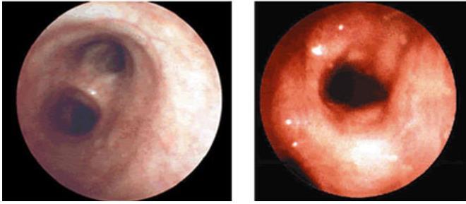
Assisting Technologies
A range of assisting technologies currently exist that can further improve on the effectiveness of short-term bronchodilator relievers. One such technology is the use of a spacer. As shown in Diagram 6, spacers work by first dispersing the bronchodilator into the air, making the inhalation more gradual, resulting in more of the medication getting into the lungs and airways where it is most effective (Asthma Australia 2021). Another method of short-acting bronchodilator delivery is through a nebulizer, where the bronchodilator is converted into a fine mist that can be inhaled normally. This method of delivery is employed on individuals who find inhaler devices difficult to use or have anatomical reasons (Asthma Australia 2021).

However, studies have shown that nebulizers are less effective in delivery of medicine compared to inhalers with a spacer. In a data review conducted by Christopher J Cates, Emma J Welsh and Brian H Rowe, it was found that in the emergency department when children were presented for severe exacerbations of asthma, the average length of stay using a nebulizer for treatment was 103 minutes, whilst the average length of stay using a spacer and reliever was 73 minutes. Overall, spacers are an addition onto relievers that will improve their effectiveness through improving the delivery of the short-acting bronchodilator into the airways and lungs.

149
Diagram 5: Left image shows a normal airway, and right image shows an asthmatic airway narrowed due to inflammation. Through use of bronchodilators, the airways would return to a state like the left image (Bronchial asthma image n.d.),
Diagram 6: Diagram showing the difference in bronchodilator distribution in the body, when using a spacer and not using a spacer on the reliever (Spacer, 2021)
Conclusion
Based on the evidence found in this study, it can be concluded that short-acting bronchodilators are an effective method of treatment for exacerbated asthma symptoms. Furthermore, their effectiveness can be improved by utilising spacer technology.
Bibliography
Abosamak, N & Shahin, M 2021, Beta 2 Receptor Agonists/Antagonists, viewed 8 May 2022, <https://www.ncbi.nlm.nih.gov/books/NBK559069/#:~:text=Beta%202%20receptors%20are %20predominantly,%2C%20lymphocytes%2C%20and%20skeletal%20muscles.>.
Almadhoun, K & Sharma, S 2021, Bronchodilators, viewed 6 May 2022, <https://www.ncbi.nlm.nih.gov/books/NBK519028/>.
Asthma Australia 2021, Asthma Puffers & Relievers, viewed 8 May 2022, <https://asthma.org.au/treatment-diagnosis/medicines-and-devices/relievers/>.
Asthma Australia 2021, Asthma Triggers and Causes, viewed 25 March 2022, <https://asthma.org.au/about-asthma/triggers/>.
Asthma Australia 2021, History, viewed 8 May 2022, <https://asthma.org.au/about-us/history/>.
Asthma Australia 2021, Spirometry, viewed 8 May 2022, <https://asthma.org.au/aboutasthma/understandingasthma/spirometry/#:~:text=Spirometry%20measures%20the%20amount%20of,confirm%20 whether%20you%20have%20asthma>.
Asthma Inhalers used in Australia 2021, Image, Asthma Australia, viewed 8 May 2022, <https://asthma.org.au/treatment-diagnosis/medicines-and-devices/relievers/>.
Asthmatic Airway Diagram 2014, Diagram, Harvard Health, viewed 29 April 2022, <https://www.2minutemedicine.com/patient-basics-asthma/>.
Australian Institute of Health and Welfare 2019, National asthma indicators – an interactive overview, viewed 9 May 2022, <https://www.aihw.gov.au/reports/chronic-respiratoryconditions/asthma-monitoring-based-on-current-indicators/contents/indicators/indicator-10costs-of-asthma>.
Australian Institute of Health and Welfare 2020, Asthma, Australian Government, viewed 29 April 2022, <https://www.aihw.gov.au/reports/chronic-respiratoryconditions/asthma/contents/asthma>.
Bronchial asthma image n.d., Photograph - bronchoscopy, Asthma Initiative of Michigan, viewed 31 March 2022, <https://getasthmahelp.org/asthma-diagnosis-classification-adults.aspx>.
Cates, CJ, Welsh, EJ & Rowe, BH 2013, Holding chambers (spacers) versus nebulisers for beta‐agonist treatment of acute asthma, viewed 9 May 2022, <https://www.ncbi.nlm.nih.gov/pmc/articles/PMC7032675/>.
Global Initiative for Asthma (GINA) 2021, GINA Full Report 2021, viewed 7 April 2022, <https://ginasthma.org/wp-content/uploads/2021/05/GINA-Main-Report-2021-V2WMS.pdf>.
Janson, C, et al, 2019, Bronchodilator reversibility in asthma and COPD: findings from three large population studies, PDF, viewed 9 May 2022, <chromeextension://efaidnbmnnnibpcajpcglclefindmkaj/https://erj.ersjournals.com/content/erj/54/3 /1900561.full.pdf>.
Pharmacy Online 2022, Ventolin CFC-Free Inhaler 100mcg x 200 doses, viewed 9 May 2022, <https://www.pharmacyonline.com.au/ventolin-cfc-free-inhaler-100mcg-x-200-dose>.
Ritchie, H & Roser, M 2022, Outdoor Air Pollution, viewed 25 March 2022, <https://ourworldindata.org/outdoor-air-pollution#how-are-deaths-from-outdoor-air-pollutionchanging>
Sinyor, B & Perez, LC 2021, Pathophysiology of Asthma, viewed 28 April 2022, <https://www.ncbi.nlm.nih.gov/books/NBK551579/>.
Souza-Machado, C, et al., 2009, Rapid reduction in hospitalisations after an intervention to manage
150
severe asthma, PDF, viewed 8 May 2022, <chromeextension://efaidnbmnnnibpcajpcglclefindmkaj/https://erj.ersjournals.com/content/erj/35/3 /515.full.pdf>.
Spacer 2021, Photograph, Asthma Australia, viewed 8 May 2022, <https://asthma.org.au/treatmentdiagnosis/medicines-and-devices/devices/>.
Syed, SA et al. 2021, Short-Term Effect of Inhaled Salbutamol on Heart Rate in Healthy Volunteers, viewed 8 May 2022, <https://www.ncbi.nlm.nih.gov/pmc/articles/PMC8018588/#:~:text=Salbutamol%20causes% 20an%20increase%20in,adrenergic%20receptors%20of%20the%20heart%2CZA>.
Thiadens, HA, et al, 1999, Can peak expiratory flow measurements reliably identify the presence of airway obstruction and bronchodilator response as assessed by FEV1 in primary care patients presenting with a persistent cough?, PDF, viewed 9 May 2022, <chromeextension://efaidnbmnnnibpcajpcglclefindmkaj/https://thorax.bmj.com/content/thoraxjnl/5 4/12/1055.full.pdf>.
World Health Organisation 2021, Asthma, viewed 25 March 2022, <https://www.who.int/newsroom/fact-sheets/detail/asthma>.
151
152
