Facial Emotion Detection Milestone 1
10/19/22, 9: 59 AMReference_Notebook_Facial_Emotion_Detection_Milestone+1 (2) Page 1 of 26file:///Users/jeffreydavis/Desktop/Applied%20Data%20Science/Projec…Reference_Notebook_Facial_Emotion_Detection_Milestone+1%20(2).html
Problem Definition
The context:
In many applications that involve safety, customer service, and mental heath the ability to recognize emotions and expressions is useful to understand if a customer is enjoying their experience, if a driver is in a poor mental state, or if a user is suffering from depression.
The objectives:
The objective is to use Deep Learning techniques to develop a computer vision model that can accurately detect facial expressions, which are useful for follow-on applications of emotion detection. The algorithm will provide a multi-output classifications emotions from expressions from facial expressions.
The key questions: What are the key questions that need to be answered?
How well identified and organized is the data?
How many different expressions are represented?
How accurate must the model be to be effective?
Is using CNN going to be move effective than an ANN?
The problem formulation: Can a machine learning model be able to identify facial expressions accurately enough to be effective for follow on applications to determine emotions.
About the dataset
The data set consists of 3 folders, i.e., 'test', 'train', and 'validation'. Each of these folders has four subfolders:
‘happy’: Images of people who have happy facial expressions. ‘sad’: Images of people with sad or upset facial expressions. ‘surprise’: Images of people who have shocked or surprised facial expressions. ‘neutral’: Images of people showing no prominent emotion in their facial expression at all.
10/19/22, 9: 59 AMReference_Notebook_Facial_Emotion_Detection_Milestone+1 (2) Page 2 of 26file:///Users/jeffreydavis/Desktop/Applied%20Data%20Science/Projec…Reference_Notebook_Facial_Emotion_Detection_Milestone+1%20(2).html
Important Notes
This notebook can be considered a guide to refer to while solving the problem. The evaluation will be as per the Rubric shared for each Milestone. Unlike previous courses, it does not follow the pattern of the graded questions in different sections. This notebook would give you a direction on what steps need to be taken to get a feasible solution to the problem. Please note that this is just one way of doing this. There can be other 'creative' ways to solve the problem, and we encourage you to feel free and explore them as an 'optional' exercise.
In the notebook, there are markdown cells called Observations and Insights. It is a good practice to provide observations and extract insights from the outputs.
The naming convention for different variables can vary. Please consider the code provided in this notebook as a sample code.
All the outputs in the notebook are just for reference and can be different if you follow a different approach.
There are sections called Think About It in the notebook that will help you get a better understanding of the reasoning behind a particular technique/step. Interested learners can take alternative approaches if they want to explore different techniques.
Mounting the Drive
NOTE: Please use Google Colab from your browser for this notebook. Google.colab is NOT a library that can be downloaded locally on your device.
Importing the Libraries
10/19/22, 9: 59 AMReference_Notebook_Facial_Emotion_Detection_Milestone+1 (2) Page 3 of 26file:///Users/jeffreydavis/Desktop/Applied%20Data%20Science/Projec…Reference_Notebook_Facial_Emotion_Detection_Milestone+1%20(2).html
Mounted at /content/drive
In [ ]: # Mounting the drive from google.colab import drive drive.mount('/content/drive')
In [ ]: import zipfile import matplotlib.pyplot as plt import numpy as np import pandas as pd import seaborn as sns import os
# Importing Deep Learning Libraries from tensorflow.keras.preprocessing.image import load_img, img_to_array from tensorflow.keras.preprocessing.image import ImageDataGenerator from tensorflow.keras.layers import Dense, Input, Dropout, GlobalAveragePooling2D from tensorflow.keras.models import Model, Sequential from tensorflow.keras.optimizers import Adam, SGD, RMSprop
Let us load the data
Note:
You must download the dataset from the link provided on Olympus and upload the same on your Google drive before executing the code in the next cell.
In case of any error, please make sure that the path of the file is correct as the path may be different for you.
In [ ]: # Storing the path of the data file from the Google drive path = '/content/drive/MyDrive/Colab_Notebooks/Applied_Data_Science/Deep_Learning/Facial_emotion_images.zip'
# The data is provided as a zip file so we need to extract the files from the zip with zipfile.ZipFile(path, 'r') as zip_ref: zip_ref.extractall()
In [ ]: picture_size = 48 folder_path = "Facial_emotion_images/"
Visualizing our Classes
Let's look at our classes.
Write down your observation for each class. What do you think can be a unique feature of each emotion, that separates it from the remaining classes?
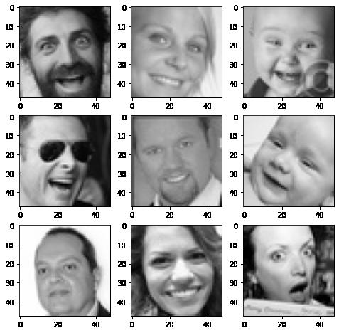
Happy
10/19/22, 9: 59 AMReference_Notebook_Facial_Emotion_Detection_Milestone+1 (2) Page 4 of 26file:///Users/jeffreydavis/Desktop/Applied%20Data%20Science/Projec…Reference_Notebook_Facial_Emotion_Detection_Milestone+1%20(2).html
In [ ]: expression = 'happy' plt.figure(figsize= (8,8)) for i in range(1, 10, 1): plt.subplot(3, 3, i)
img = load_img(folder_path + "train/" + expression + "/" + os.listdir(folder_path + "train/" + expression)[i], target_size plt.imshow(img) plt.show()
Observations and Insights:
The dataset looks representitive of several types of happy expressions; however, these intial representations do not have many skin tone differences. My concern at this point is overfitting an accurate training set. I will keep a close eye on signs of overfitting. I belive that the eyes, in combination with the up-turn at the corner of the mouth, as well as raised cheeks will be some of the defining features.
10/19/22, 9: 59 AMReference_Notebook_Facial_Emotion_Detection_Milestone+1 (2) Page 5 of 26file:///Users/jeffreydavis/Desktop/Applied%20Data%20Science/Projec…Reference_Notebook_Facial_Emotion_Detection_Milestone+1%20(2).html
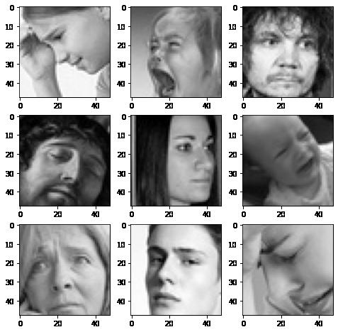
Sad
In [ ]: # Write your code to visualize images from the class 'sad'. expression = 'sad' plt.figure(figsize= (8,8)) for i in range(1, 10, 1): plt.subplot(3, 3, i) img = load_img(folder_path + "train/" + expression + "/" + os.listdir(folder_path + "train/" + expression)[i], target_size plt.imshow(img) plt.show()
10/19/22, 9: 59 AMReference_Notebook_Facial_Emotion_Detection_Milestone+1 (2) Page 6 of 26file:///Users/jeffreydavis/Desktop/Applied%20Data%20Science/Projec…Reference_Notebook_Facial_Emotion_Detection_Milestone+1%20(2).html
Observations and Insights:
The angry faces seem to have several distinguisihing features from the happy expressions. At fist glance it seems representive of several facial structures, skin tones, and facial features. The downturn of the eyes, pouty lips and crincles in forhead may be the most defining features.
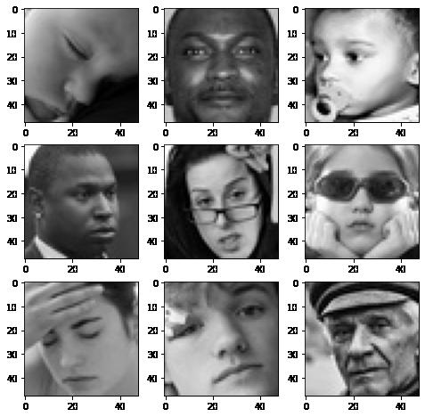
Neutral
In [ ]: # Write your code to visualize images from the class 'neutral'. expression = 'neutral'
plt.figure(figsize= (8,8)) for i in range(1, 10, 1): plt.subplot(3, 3, i)
img = load_img(folder_path + "train/" + expression + "/" + os.listdir(folder_path + "train/" + expression)[i], target_size plt.imshow(img) plt.show()
10/19/22, 9: 59 AMReference_Notebook_Facial_Emotion_Detection_Milestone+1 (2) Page 7 of 26file:///Users/jeffreydavis/Desktop/Applied%20Data%20Science/Projec…Reference_Notebook_Facial_Emotion_Detection_Milestone+1%20(2).html
Observations and Insights:
At first glance these images are going to be difficut to distingues between other emotions. It may be nessassary to use data augmentation. It is clear looking at this that using CNN will most likely be more effective than ANN. What will define this from happy, will likely be the lack of major emotion on other parts of the face. No tightness in the eyebrows, for example, will differenetiate the faces from sad faces. The lack of cheeks rising to the eyes will likely differentiate them from happy faces.
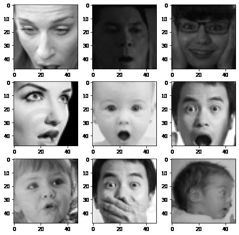
Surprised
10/19/22, 9: 59 AMReference_Notebook_Facial_Emotion_Detection_Milestone+1 (2) Page 8 of 26file:///Users/jeffreydavis/Desktop/Applied%20Data%20Science/Projec…Reference_Notebook_Facial_Emotion_Detection_Milestone+1%20(2).html
In [ ]: # Write your code to visualize images from the class 'surprise'. expression = 'surprise' plt.figure(figsize= (8,8)) for i in range(1, 10, 1): plt.subplot(3, 3, i)
img = load_img(folder_path + "train/" + expression + "/" + os.listdir(folder_path + "train/" + expression)[i], target_size plt.imshow(img) plt.show()
Observations and Insights:
The data set looks clean. All immages have the same dimensions accross datasets. The looks of surprise will probably be destiguished by the widness of the eyes, and raising of the eyebrows, along with gaping mouths. All of the images (accross all data sets) vary in size and are positionally different on within the frame of the picture.
10/19/22, 9: 59 AMReference_Notebook_Facial_Emotion_Detection_Milestone+1 (2) Page 9 of 26file:///Users/jeffreydavis/Desktop/Applied%20Data%20Science/Projec…Reference_Notebook_Facial_Emotion_Detection_Milestone+1%20(2).html
Checking Distribution of Classes
In [ ]: # Getting count of images in each folder within our training path num_happy = len(os.listdir(folder_path + "train/happy")) print("Number of images in the class 'happy': ", num_happy)
num_sad = len(os.listdir(folder_path+ "train/sad")) print("Number of images in the calss 'sad': ",num_sad)
num_neutral = len(os.listdir(folder_path+ "train/neutral")) print("Number of images in the calss 'neutral': ",num_neutral)
num_surprise = len(os.listdir(folder_path+ "train/surprise")) print("Number of images in the calss 'surprise': ",num_surprise)
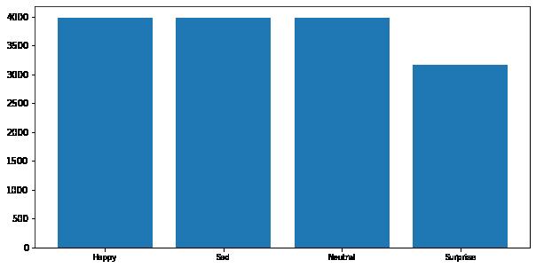
Number of images in the class 'happy': 3976
Number of images in the calss 'sad': 3982
Number of images in the calss 'neutral': 3978
Number of images in the calss 'surprise': 3173
In [ ]: # Code to plot histogram plt.figure(figsize = (10, 5))
data = {'Happy': num_happy, 'Sad': num_sad, 'Neutral': num_neutral, 'Surprise' df = pd.Series(data) plt.bar(range(len(df)), df.values, align = 'center') plt.xticks(range(len(df)), df.index.values, size = 'small') plt.show()
10/19/22, 9: 59 AMReference_Notebook_Facial_Emotion_Detection_Milestone+1 (2) Page 10 of 26file:///Users/jeffreydavis/Desktop/Applied%20Data%20Science/Projec…eference_Notebook_Facial_Emotion_Detection_Milestone+1%20(2).html
Observations and Insights:
There are substantially less examples of surprise in the training data, by ~1000 images. This may have some effect on the efficacy of the training. Once we build initial models we will want to build a confusion matrix to identify if there is a loss of efficacy due to the reduction of surprise. We can attempt to correct the issue through undersampling and data augmentation.
Normalizing the data may also reduce the effect.
Think About It:
Are the classes equally distributed? If not, do you think the imbalance is too high? Will it be a problem as we progress?
Are there any Exploratory Data Analysis tasks that we can do here? Would they provide any meaningful insights?
Creating our Data Loaders
In this section, we are creating data loaders that we will use as inputs to our Neural Network. A sample of the required code has been given with respect to the training data. Please create the data loaders for validation and test set accordingly.
You have two options for the color_mode. You can set it to color_mode = 'rgb' or color_mode = 'grayscale'. You will need to try out both and see for yourself which one gives better performance.
10/19/22, 9: 59 AMReference_Notebook_Facial_Emotion_Detection_Milestone+1 (2) Page 11 of 26file:///Users/jeffreydavis/Desktop/Applied%20Data%20Science/Projec…eference_Notebook_Facial_Emotion_Detection_Milestone+1%20(2).html
In [ ]: batch_size = 32 img_size = 48
datagen_train = ImageDataGenerator(horizontal_flip = True, brightness_range=(0.,2.), rescale=1./255, shear_range=0.3)
train_set = datagen_train.flow_from_directory(folder_path + "train", target_size = (img_size, img_size color_mode = 'rgb', batch_size = batch_size, class_mode = 'categorical', shuffle = True)
datagen_validation = ImageDataGenerator(horizontal_flip = True, brightness_range=(0.,2.), rescale=1./255, shear_range=0.3)
validation_set = datagen_validation.flow_from_directory(folder_path + "validation" target_size = (img_size, img_size color_mode = 'rgb', batch_size = batch_size, class_mode = 'categorical', shuffle = True)
datagen_test = ImageDataGenerator(horizontal_flip = True, brightness_range=(0.,2.), rescale=1./255, shear_range=0.3)
test_set = datagen_test.flow_from_directory(folder_path + "test", target_size = (img_size, img_size color_mode = 'rgb', batch_size = batch_size, class_mode = 'categorical', shuffle = True)
Found 15109 images belonging to 4 classes. Found 4977 images belonging to 4 classes. Found 128 images belonging to 4 classes.
Model Building
10/19/22, 9: 59 AMReference_Notebook_Facial_Emotion_Detection_Milestone+1 (2) Page 12 of 26file:///Users/jeffreydavis/Desktop/Applied%20Data%20Science/Projec…eference_Notebook_Facial_Emotion_Detection_Milestone+1%20(2).html
Think About It:
Are Convolutional Neural Networks the right approach? Should we have gone with Artificial Neural Networks instead?
What are the advantages of CNNs over ANNs and are they applicable here?
Give the fact that the images are placed in different size and spacial orientation, filter strides will maintain more fidelity and understanding about the immage prior to flattening. In turn the abilty to weight share in CNNs will provide the model with the total value of the image, rather than just a single point.
Creating the Base Neural Network
Our Base Neural network will be a fairly simple model architecture.
We want our Base Neural Network architecture to have 3 convolutional blocks. Each convolutional block must contain one Conv2D layer followed by a maxpooling layer and one Dropout layer. We can play around with the dropout ratio.
Add first Conv2D layer with 64 filters and a kernel size of 2. Use the 'same' padding and provide the input_shape = (48, 48, 3) if you are using 'rgb' color mode in your dataloader or else input shape = (48, 48, 1) if you're using 'grayscale' colormode. Use 'relu' activation
Add MaxPooling2D layer with pool size = 2.
Add a Dropout layer with a dropout ratio of 0.2.
Add a second Conv2D layer with 32 filters and a kernel size of 2. Use the 'same' padding and 'relu' activation.
Follow this up with a similar Maxpooling2D layer like above and a Dropout layer with 0.2 Dropout ratio to complete your second Convolutional Block.
Add a third Conv2D layer with 32 filters and a kernel size of 2. Use the 'same' padding and 'relu' activation. Once again, follow it up with a Maxpooling2D layer and a Dropout layer to complete your third Convolutional block.
After adding your convolutional blocks, add your Flatten layer.
Add your first Dense layer with 512 neurons. Use 'relu' activation function.
Add a Dropout layer with dropout ratio of 0.4.
Add your final Dense Layer with 4 neurons and 'softmax' activation function
Print your model summary
10/19/22, 9: 59 AMReference_Notebook_Facial_Emotion_Detection_Milestone+1 (2) Page 13 of 26file:///Users/jeffreydavis/Desktop/Applied%20Data%20Science/Projec…eference_Notebook_Facial_Emotion_Detection_Milestone+1%20(2).html
In [ ]: # Initializing a Sequential Model model1 = Sequential()
# Add the first Convolutional block model1.add(Conv2D(64, (2, 2), padding = 'same', activation = 'relu', input_shape model1.add(MaxPooling2D(2, 2)) model1.add(Dropout(rate = 0.2))
# Add the second Convolutional block model1.add(Conv2D(32, (2, 2), padding = 'same', activation = 'relu')) model1.add(MaxPooling2D(2, 2)) model1.add(Dropout(rate = 0.2))
# Add the third Convolutional block model1.add(Conv2D(32, (2, 2), padding = 'same', activation = 'relu')) model1.add(MaxPooling2D(2, 2)) model1.add(Dropout (rate = 0.2))
# Add the Flatten layer model1.add(Flatten())
# Add the first Dense layer model1.add(Dense(512, activation = 'relu')) model1.add(Dropout (rate = 0.4))
# Add the Final layer model1.add(Dense(4, activation = 'softmax'))
model1.summary()
10/19/22, 9: 59 AMReference_Notebook_Facial_Emotion_Detection_Milestone+1 (2) Page 14 of 26file:///Users/jeffreydavis/Desktop/Applied%20Data%20Science/Projec…eference_Notebook_Facial_Emotion_Detection_Milestone+1%20(2).html
Model: "sequential_4"
Layer (type) Output Shape Param # =================================================================
conv2d_13 (Conv2D) (None, 48, 48, 64) 832
max_pooling2d_13 (MaxPoolin (None, 24, 24, 64) 0 g2D)
dropout_12 (Dropout) (None, 24, 24, 64) 0 conv2d_14 (Conv2D) (None, 24, 24, 32) 8224
max_pooling2d_14 (MaxPoolin (None, 12, 12, 32) 0 g2D)
dropout_13 (Dropout) (None, 12, 12, 32) 0 conv2d_15 (Conv2D) (None, 12, 12, 32) 4128
max_pooling2d_15 (MaxPoolin (None, 6, 6, 32) 0 g2D)
dropout_14 (Dropout) (None, 6, 6, 32) 0 flatten_4 (Flatten) (None, 1152) 0 dense_7 (Dense) (None, 512) 590336
dropout_15 (Dropout) (None, 512) 0 dense_8 (Dense) (None, 4) 2052
Compiling and Training the Model
10/19/22, 9: 59 AMReference_Notebook_Facial_Emotion_Detection_Milestone+1 (2) Page 15 of 26file:///Users/jeffreydavis/Desktop/Applied%20Data%20Science/Projec…eference_Notebook_Facial_Emotion_Detection_Milestone+1%20(2).html
================================================================= Total params: 605,572 Trainable params: 605,572 Non-trainable params: 0
In [ ]: from keras.callbacks import ModelCheckpoint, EarlyStopping, ReduceLROnPlateau checkpoint = ModelCheckpoint("./model1.h5", monitor='val_acc', verbose=1, save_best_only early_stopping = EarlyStopping(monitor = 'val_loss', min_delta = 0, patience = 3, verbose = 1, restore_best_weights = True )
reduce_learningrate = ReduceLROnPlateau(monitor = 'val_loss', factor = 0.2, patience = 3, verbose = 1, min_delta = 0.0001)
callbacks_list = [early_stopping, checkpoint, reduce_learningrate] epochs = 20
In [ ]: # Write your code to compile your model1. Use categorical crossentropy as your loss model1.compile(optimizer = Adam(learning_rate = 0.001), loss = 'categorical_crossentropy'
In [ ]: # Write your code to fit your model1. Use train_set as your training data and validation_set history = model1.fit(x= train_set, validation_data = validation_set, epochs
Epoch 1/20
473/473 [==============================] - 94s 197ms/step - loss: 1.3421 - a ccuracy: 0.3237 - val_loss: 1.2627 - val_accuracy: 0.4316
Epoch 2/20
473/473 [==============================] - 96s 203ms/step - loss: 1.2065 - a ccuracy: 0.4530 - val_loss: 1.1329 - val_accuracy: 0.5164 Epoch 3/20
473/473 [==============================] - 90s 191ms/step - loss: 1.1079 - a ccuracy: 0.5133 - val_loss: 1.0343 - val_accuracy: 0.5558
Epoch 4/20
473/473 [==============================] - 89s 187ms/step - loss: 1.0679 - a ccuracy: 0.5333 - val_loss: 1.0167 - val_accuracy: 0.5704
Epoch 5/20
473/473 [==============================] - 91s 192ms/step - loss: 1.0276 - a ccuracy: 0.5538 - val_loss: 0.9883 - val_accuracy: 0.5746 Epoch 6/20
473/473 [==============================] - 91s 193ms/step - loss: 1.0055 - a ccuracy: 0.5648 - val_loss: 0.9385 - val_accuracy: 0.6030
Epoch 7/20
473/473 [==============================] - 92s 194ms/step - loss: 0.9851 - a ccuracy: 0.5733 - val_loss: 0.9105 - val_accuracy: 0.6205
Epoch 8/20
473/473 [==============================] - 89s 189ms/step - loss: 0.9631 - a ccuracy: 0.5824 - val_loss: 0.8975 - val_accuracy: 0.6281
10/19/22, 9: 59 AMReference_Notebook_Facial_Emotion_Detection_Milestone+1 (2) Page 16 of 26file:///Users/jeffreydavis/Desktop/Applied%20Data%20Science/Projec…eference_Notebook_Facial_Emotion_Detection_Milestone+1%20(2).html
Epoch 9/20
473/473 [==============================] - 91s 191ms/step - loss: 0.9560 - a ccuracy: 0.5887 - val_loss: 0.8771 - val_accuracy: 0.6397
Epoch 10/20
473/473 [==============================] - 88s 186ms/step - loss: 0.9337 - a ccuracy: 0.5961 - val_loss: 0.9312 - val_accuracy: 0.6096
Epoch 11/20
473/473 [==============================] - 89s 188ms/step - loss: 0.9223 - a ccuracy: 0.6058 - val_loss: 0.8616 - val_accuracy: 0.6428
Epoch 12/20
473/473 [==============================] - 90s 191ms/step - loss: 0.9148 - a ccuracy: 0.6053 - val_loss: 0.8454 - val_accuracy: 0.6574
Epoch 13/20
473/473 [==============================] - 99s 208ms/step - loss: 0.9031 - a ccuracy: 0.6184 - val_loss: 0.8526 - val_accuracy: 0.6562
Epoch 14/20
473/473 [==============================] - 98s 207ms/step - loss: 0.8960 - a ccuracy: 0.6208 - val_loss: 0.8474 - val_accuracy: 0.6522
Epoch 15/20
473/473 [==============================] - 91s 192ms/step - loss: 0.8766 - a ccuracy: 0.6282 - val_loss: 0.8141 - val_accuracy: 0.6572 Epoch 16/20
473/473 [==============================] - 89s 187ms/step - loss: 0.8756 - a ccuracy: 0.6286 - val_loss: 0.8065 - val_accuracy: 0.6769
Epoch 17/20
473/473 [==============================] - 89s 188ms/step - loss: 0.8638 - a ccuracy: 0.6366 - val_loss: 0.8321 - val_accuracy: 0.6558 Epoch 18/20
473/473 [==============================] - 89s 188ms/step - loss: 0.8559 - a ccuracy: 0.6358 - val_loss: 0.8057 - val_accuracy: 0.6755
Epoch 19/20
473/473 [==============================] - 90s 191ms/step - loss: 0.8464 - a ccuracy: 0.6438 - val_loss: 0.8057 - val_accuracy: 0.6671 Epoch 20/20
473/473 [==============================] - 90s 191ms/step - loss: 0.8384 - a ccuracy: 0.6493 - val_loss: 0.8080 - val_accuracy: 0.6699
Evaluating the Model on the Test Set
10/19/22, 9: 59 AMReference_Notebook_Facial_Emotion_Detection_Milestone+1 (2) Page 17 of 26file:///Users/jeffreydavis/Desktop/Applied%20Data%20Science/Projec…eference_Notebook_Facial_Emotion_Detection_Milestone+1%20(2).html
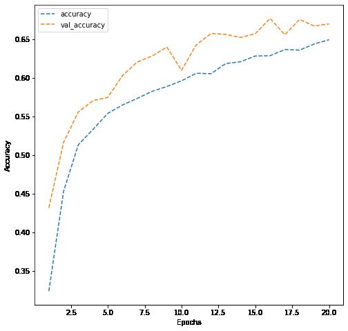
In [ ]: # Write your code to evaluate your model on test data. dict_hist = history.history list_ep = [i for i in range(1, 21)] plt.figure(figsize = (8, 8)) plt.plot(list_ep, dict_hist['accuracy'], ls = '--' , label = 'accuracy') plt.plot(list_ep, dict_hist['val_accuracy'], ls = '--' , label = 'val_accuracy' plt.ylabel('Accuracy') plt.xlabel('Epochs') plt.legend() plt.show()
10/19/22, 9: 59 AMReference_Notebook_Facial_Emotion_Detection_Milestone+1 (2) Page 18 of 26file:///Users/jeffreydavis/Desktop/Applied%20Data%20Science/Projec…eference_Notebook_Facial_Emotion_Detection_Milestone+1%20(2).html
Observations and Insights:
Results are not acceptable, althought validation accuracy was running parallel to training accuracy, the top result was ~67% accurate, clearly not meeting the needs of any potential follow-up application. I tested the models with both rgb and greyscale. The results are almost identical.
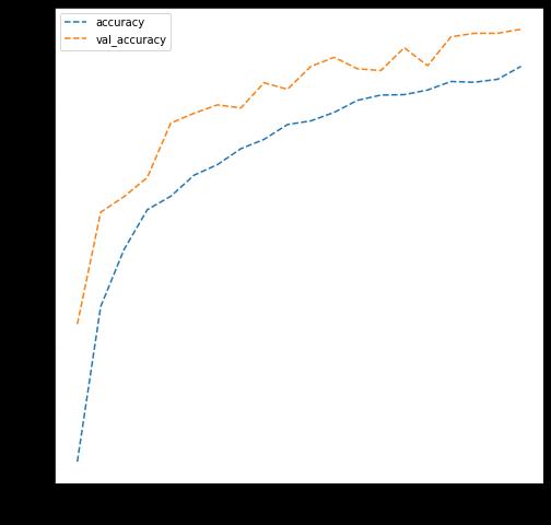
Grayscale:
Creating the second Convolutional Neural Network
10/19/22, 9: 59 AMReference_Notebook_Facial_Emotion_Detection_Milestone+1 (2) Page 19 of 26file:///Users/jeffreydavis/Desktop/Applied%20Data%20Science/Projec…eference_Notebook_Facial_Emotion_Detection_Milestone+1%20(2).html
In the second Neural network, we will add a few more Convolutional blocks. We will also use Batch Normalization layers.
This time, each Convolutional block will have 1 Conv2D layer, followed by a BatchNormalization, LeakuRelU, and a MaxPooling2D layer. We are not adding any Dropout layer this time.
Add first Conv2D layer with 256 filters and a kernel size of 2. Use the 'same' padding and provide the input_shape = (48, 48, 3) if you are using 'rgb' color mode in your dataloader or else input shape = (48, 48, 1) if you're using 'grayscale' colormode. Use 'relu' activation.
Add your BatchNormalization layer followed by a LeakyRelU layer with Leaky ReLU parameter of 0.1
Add MaxPooling2D layer with pool size = 2.
Add a second Conv2D layer with 128 filters and a kernel size of 2. Use the 'same' padding and 'relu' activation.
Follow this up with a similar BatchNormalization, LeakyRelU, and Maxpooling2D layer like above to complete your second Convolutional Block.
Add a third Conv2D layer with 64 filters and a kernel size of 2. Use the 'same' padding and 'relu' activation. Once again, follow it up with a BatchNormalization, LeakyRelU, and Maxpooling2D layer to complete your third Convolutional block.
Add a fourth block, with the Conv2D layer having 32 filters
After adding your convolutional blocks, add your Flatten layer.
Add your first Dense layer with 512 neurons. Use 'relu' activation function.
Add the second Dense Layer with 128 neurons and use 'relu' activation function.
Add your final Dense Layer with 4 neurons and 'softmax' activation function
Print your model summary
10/19/22, 9: 59 AMReference_Notebook_Facial_Emotion_Detection_Milestone+1 (2) Page 20 of 26file:///Users/jeffreydavis/Desktop/Applied%20Data%20Science/Projec…eference_Notebook_Facial_Emotion_Detection_Milestone+1%20(2).html
In [ ]: # Creating sequential model model2 = Sequential()
# Add the first Convolutional block model2.add(Conv2D(256, (2, 2), padding = 'same', input_shape = (48, 48, 3))) model2.add(BatchNormalization()) model2.add(LeakyReLU(alpha = 0.1)) model2.add(MaxPooling2D(2, 2))
# Add the second Convolutional block model2.add(Conv2D(128, (2, 2), padding = 'same')) model2.add(BatchNormalization()) model2.add(LeakyReLU(alpha = 0.1)) model2.add(MaxPooling2D(2, 2))
# Add the third Convolutional block model2.add(Conv2D(64, (2, 2), padding = 'same')) model2.add(BatchNormalization()) model2.add(LeakyReLU(alpha = 0.1)) model2.add(MaxPooling2D(2, 2))
# Add the fourth Convolutional block model2.add(Conv2D(32, (2, 2), padding = 'same')) model2.add(BatchNormalization()) model2.add(LeakyReLU(alpha = 0.1)) model2.add(MaxPooling2D(2, 2))
# Add the Flatten layer model2.add(Flatten())
# Adding the Dense layers model2.add(Dense(512, activation = 'relu')) model2.add(Dense(128, activation = 'relu')) model2.add(Dense(4, activation = 'softmax')) model2.summary()
Model: "sequential_6"
Layer (type) Output Shape Param # ================================================================= conv2d_20 (Conv2D) (None, 48, 48, 256) 3328 batch_normalization_8 (Batc (None, 48, 48, 256) 1024 hNormalization)
leaky_re_lu_8 (LeakyReLU) (None, 48, 48, 256) 0
10/19/22, 9: 59 AMReference_Notebook_Facial_Emotion_Detection_Milestone+1 (2) Page 21 of 26file:///Users/jeffreydavis/Desktop/Applied%20Data%20Science/Projec…eference_Notebook_Facial_Emotion_Detection_Milestone+1%20(2).html
max_pooling2d_20 (MaxPoolin (None, 24, 24, 256) 0 g2D)
conv2d_21 (Conv2D) (None, 24, 24, 128) 131200
batch_normalization_9 (Batc (None, 24, 24, 128) 512 hNormalization)
leaky_re_lu_9 (LeakyReLU) (None, 24, 24, 128) 0
max_pooling2d_21 (MaxPoolin (None, 12, 12, 128) 0 g2D)
conv2d_22 (Conv2D) (None, 12, 12, 64) 32832
batch_normalization_10 (Bat (None, 12, 12, 64) 256 chNormalization)
leaky_re_lu_10 (LeakyReLU) (None, 12, 12, 64) 0
max_pooling2d_22 (MaxPoolin (None, 6, 6, 64) 0 g2D)
conv2d_23 (Conv2D) (None, 6, 6, 32) 8224
batch_normalization_11 (Bat (None, 6, 6, 32) 128 chNormalization)
leaky_re_lu_11 (LeakyReLU) (None, 6, 6, 32) 0 max_pooling2d_23 (MaxPoolin (None, 3, 3, 32) 0 g2D)
flatten_6 (Flatten) (None, 288) 0 dense_12 (Dense) (None, 512) 147968 dense_13 (Dense) (None, 128) 65664 dense_14 (Dense) (None, 4) 516
10/19/22, 9: 59 AMReference_Notebook_Facial_Emotion_Detection_Milestone+1 (2) Page 22 of 26file:///Users/jeffreydavis/Desktop/Applied%20Data%20Science/Projec…eference_Notebook_Facial_Emotion_Detection_Milestone+1%20(2).html
================================================================= Total params: 391,652 Trainable params: 390,692 Non-trainable params: 960
Compiling and Training the Model
Hint: Take reference from the code we used in the previous model for Compiling and Training the Model.
In [ ]: from keras.callbacks import ModelCheckpoint, EarlyStopping, ReduceLROnPlateau checkpoint = ModelCheckpoint("./model2.h5", monitor='val_loss', verbose = 1, ##Changing parameters did not make sense, as we already are testing several changes early_stopping = EarlyStopping(monitor = 'val_loss', min_delta = 0, patience = 3, verbose = 1, restore_best_weights = True )
reduce_learningrate = ReduceLROnPlateau(monitor = 'val_loss', factor = 0.2, patience = 3, verbose = 1, min_delta = 0.0001)
callbacks_list = [early_stopping, checkpoint, reduce_learningrate] epochs = 20
In [ ]: # Write your code to compile your model2. Use categorical crossentropy as the loss model2.compile(optimizer = Adam(learning_rate = 0.001), loss = 'categorical_crossentropy'
In [ ]: history = model2.fit(x= train_set, validation_data = validation_set, batch_size # Write your code to fit your model2. Use train_set as the training data and validation_set # set a batch size of 32 to try and reduce compute time, there was little effect.
Epoch 1/20
473/473 [==============================] - 487s 1s/step - loss: 1.1187 - acc uracy: 0.4927 - val_loss: 1.0121 - val_accuracy: 0.5626 Epoch 2/20
473/473 [==============================] - 484s 1s/step - loss: 0.9738 - acc uracy: 0.5784 - val_loss: 0.9560 - val_accuracy: 0.5907 Epoch 3/20
473/473 [==============================] - 481s 1s/step - loss: 0.8976 - acc uracy: 0.6112 - val_loss: 0.9301 - val_accuracy: 0.6018
Epoch 4/20
473/473 [==============================] - 485s 1s/step - loss: 0.8615 - acc uracy: 0.6333 - val_loss: 0.8541 - val_accuracy: 0.6389
Epoch 5/20
473/473 [==============================] - 482s 1s/step - loss: 0.8169 - acc uracy: 0.6505 - val_loss: 0.8217 - val_accuracy: 0.6520
Epoch 6/20
10/19/22, 9: 59 AMReference_Notebook_Facial_Emotion_Detection_Milestone+1 (2) Page 23 of 26file:///Users/jeffreydavis/Desktop/Applied%20Data%20Science/Projec…eference_Notebook_Facial_Emotion_Detection_Milestone+1%20(2).html
473/473 [==============================] - 482s 1s/step - loss: 0.7922 - acc uracy: 0.6683 - val_loss: 0.9359 - val_accuracy: 0.6048
Epoch 7/20
473/473 [==============================] - 481s 1s/step - loss: 0.7816 - acc uracy: 0.6713 - val_loss: 0.8136 - val_accuracy: 0.6568
Epoch 8/20
473/473 [==============================] - 482s 1s/step - loss: 0.7537 - acc uracy: 0.6851 - val_loss: 0.8126 - val_accuracy: 0.6635
Epoch 9/20
473/473 [==============================] - 483s 1s/step - loss: 0.7379 - acc uracy: 0.6906 - val_loss: 0.7948 - val_accuracy: 0.6661
Epoch 10/20
473/473 [==============================] - 480s 1s/step - loss: 0.7189 - acc uracy: 0.6985 - val_loss: 0.8349 - val_accuracy: 0.6641
Epoch 11/20
473/473 [==============================] - 479s 1s/step - loss: 0.6977 - acc uracy: 0.7067 - val_loss: 0.8288 - val_accuracy: 0.6552
Epoch 12/20
473/473 [==============================] - 485s 1s/step - loss: 0.6823 - acc uracy: 0.7146 - val_loss: 0.7521 - val_accuracy: 0.7000
Epoch 13/20
473/473 [==============================] - 485s 1s/step - loss: 0.6788 - acc uracy: 0.7173 - val_loss: 0.8540 - val_accuracy: 0.6673
Epoch 14/20
473/473 [==============================] - 477s 1s/step - loss: 0.6579 - acc uracy: 0.7256 - val_loss: 0.8309 - val_accuracy: 0.6659
Epoch 15/20
473/473 [==============================] - 534s 1s/step - loss: 0.6471 - acc uracy: 0.7319 - val_loss: 0.8474 - val_accuracy: 0.6715
Epoch 16/20
473/473 [==============================] - 569s 1s/step - loss: 0.6362 - acc uracy: 0.7409 - val_loss: 0.7543 - val_accuracy: 0.6916
Epoch 17/20
473/473 [==============================] - 570s 1s/step - loss: 0.6193 - acc uracy: 0.7435 - val_loss: 0.8034 - val_accuracy: 0.6992
Epoch 18/20
473/473 [==============================] - 529s 1s/step - loss: 0.6140 - acc uracy: 0.7460 - val_loss: 0.7674 - val_accuracy: 0.6962
Epoch 19/20
473/473 [==============================] - 480s 1s/step - loss: 0.5925 - acc uracy: 0.7601 - val_loss: 0.8115 - val_accuracy: 0.6862
Epoch 20/20
473/473 [==============================] - 473s 1s/step - loss: 0.5892 - acc uracy: 0.7587 - val_loss: 0.7665 - val_accuracy: 0.7012
Evaluating the Model on the Test Set
10/19/22, 9: 59 AMReference_Notebook_Facial_Emotion_Detection_Milestone+1 (2) Page 24 of 26file:///Users/jeffreydavis/Desktop/Applied%20Data%20Science/Projec…eference_Notebook_Facial_Emotion_Detection_Milestone+1%20(2).html
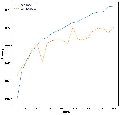
In [ ]: # Write your code to evaluate model's test performance dict_hist = history.history list_ep = [i for i in range(1, 21)] plt.figure(figsize = (8, 8)) plt.plot(list_ep, dict_hist['accuracy'], ls = '--' , label = 'accuracy') plt.plot(list_ep, dict_hist['val_accuracy'], ls = '--' , label = 'val_accuracy' plt.ylabel('Accuracy') plt.xlabel('Epochs') plt.legend() plt.show()
10/19/22, 9: 59 AMReference_Notebook_Facial_Emotion_Detection_Milestone+1 (2) Page 25 of 26file:///Users/jeffreydavis/Desktop/Applied%20Data%20Science/Projec…eference_Notebook_Facial_Emotion_Detection_Milestone+1%20(2).html
Observations and Insights:
This model barely performed better than the last, and as the training data improved the model was not improving its generalization (Validation accuracy was stuck at ~70%).
Niether of these models performed well, and the second used a considerable amount of time and compute power.
The difference in the color setting was negligable, although grayscale would remove several of the parameters. The most obvious issue is that the model is learing slowly and poorly, There are several steps we can look at from here:
chaging the parameters - including some Dropouts
Data augmentation
changing some hyper-parameters (such as learning rate)
Network structure. This model places several nerons in a thin slice of layers.
Potentially using the same number of nodes, spread accross more hidden layers. Also, the great deal of CNN did not have a noticable change on the generalization of the model, so we can try simplifying this part of the model.
Think About It:
Did the models have a satisfactory performance? If not, then what are the possible reasons?
Which Color mode showed better overall performance? What are the possible reasons? Do you think having 'rgb' color mode is needed because the images are already black and white?
**Proposed Approach**
Potential techniques: What different techniques should be explored? Data
Augmentation; Parameter and hyperparameter adjustment, deeper hidden layers. Also must keep an eye on overfitting
Overall solution design: We will work with developing a more simple CNN, with deeper parameters.
Measures of success: The measure of success is accuracy of test data. 90% or better.
10/19/22, 9: 59 AMReference_Notebook_Facial_Emotion_Detection_Milestone+1 (2) Page 26 of 26file:///Users/jeffreydavis/Desktop/Applied%20Data%20Science/Projec…eference_Notebook_Facial_Emotion_Detection_Milestone+1%20(2).html
