Advertising Channel Effects on Sales

Effects of Advertising on Sales

LVC 1 - Introduction to Supervised Learning: Regression

Context and Problem

This is a practical application project presented for the MIT Applied Data Science Course utilizing multi-variant regression to analyse advertising effectiveness and spending.

An interesting application of regression is to quantify the effect of advertisement on sales. Various channels of advertisement are newspaper, TV, radio, etc. In this case study, we will have a look at the advertising data of a company and try to see its effect on sales.

We will also try to predict the sales given the different parameters of advertising.

Data Information

The data at hand has three features about the spending on advertising and the target variable is the net sales. Attributes are: TV - Independent variable quantifying budget for TV ads Radio - Independent variable quantifying budget for radio ads News - Independent variable quantifying budget for news ads Sales - Dependent variable

Importing libraries and data

In [1]: import pandas as pd import numpy as np import numpy as np from sklearn import linear_model import matplotlib.pyplot as plt

In [2]: Ad_df = pd.read_csv('Advertising.csv') Ad_df.head()

Out[2]:

Unnamed: 0 TV Radio Newspaper Sales

0 1 230.1 37.8 69.2 22.1

1 2 44.5 39.3 45.1 10.4

3 17.2 45.9 69.3 9.3

4 151.5 41.3 58.5 18.5

5 180.8 10.8 58.4 12.9

Note: this is a fairly simple dataset with only 4 variables.

In [3]: # Dropping the first column as it is just the index Ad_df.drop(columns = 'Unnamed: 0', inplace=True)

In [4]: Ad_df

Out[4]: In [5]: Ad_df.info()

TV Radio Newspaper Sales

0 230.1 37.8 69.2 22.1 1 44.5 39.3 45.1 10.4 2 17.2 45.9 69.3 9.3 3 151.5 41.3 58.5 18.5 4 180.8 10.8 58.4 12.9 ... 195 38.2 3.7 13.8 7.6 196 94.2 4.9 8.1 9.7 197 177.0 9.3 6.4 12.8 198 283.6 42.0 66.2 25.5 199 232.1 8.6 8.7 13.4 200 rows × 4 columns

<class 'pandas.core.frame.DataFrame'>

RangeIndex: 200 entries, 0 to 199

Data columns (total 4 columns): # Column Non-Null Count Dtype --- ------ -------------- -----

0 TV 200 non-null float64

1 Radio 200 non-null float64

2 Newspaper 200 non-null float64

3 Sales 200 non-null float64

dtypes: float64(4) memory usage: 6.4 KB

Observations:

All the variables are of float data type.

There is a total of 200 samples (a small data set, but useful for a regression analysis.

Let us now start with the simple linear regression. We will use one feature at a time and have a look at the target variable.

In [6]: # Dataset is stored in a Pandas Dataframe. Taking out all the variables in a numpy Sales = Ad_df.Sales.values.reshape(len(Ad_df['Sales']), 1)

TV = Ad_df.TV.values.reshape(len(Ad_df['Sales']), 1)

Radio = Ad_df.Radio.values.reshape(len(Ad_df['Sales']), 1)

Newspaper = Ad_df.Newspaper.values.reshape(len(Ad_df['Sales']), 1)

In [7]: # Fitting a simple linear regression model with the TV feature tv_model = linear_model.LinearRegression() tv_model.fit(TV, Sales) coeffs_tv = np.array(list(tv_model.intercept_.flatten()) + list(tv_model.coef_ coeffs_tv = list(coeffs_tv)

# Radio feature radio_model = linear_model.LinearRegression() radio_model.fit(Radio, Sales) coeffs_radio = np.array(list(radio_model.intercept_.flatten()) + list(radio_model coeffs_radio = list(coeffs_radio)

# Newspaper feature newspaper_model = linear_model.LinearRegression() newspaper_model.fit(Newspaper, Sales) coeffs_newspaper = np.array(list(newspaper_model.intercept_.flatten()) + list coeffs_newspaper = list(coeffs_newspaper)

# Storing the above results in a dictionary and then display using a dataframe dict_Sales = {} dict_Sales["TV"] = coeffs_tv dict_Sales["Radio"] = coeffs_radio dict_Sales["Newspaper"] = coeffs_newspaper

metric_Df_SLR = pd.DataFrame(dict_Sales) metric_Df_SLR.index = ['Intercept', 'Coefficient'] metric_Df_SLR

Out[7]:

TV Radio Newspaper Intercept 7.032594 9.311638 12.351407 Coefficient 0.047537 0.202496 0.054693

In [8]: # Let us now calculate R^2 tv_rsq = tv_model.score(TV, Sales) radio_rsq = radio_model.score(Radio, Sales) newspaper_rsq = newspaper_model.score(Newspaper, Sales)

print("TV simple linear regression R-Square :", tv_rsq) print("Radio simple linear regression R-Square :", radio_rsq) print("Newspaper simple linear regression R-Square :", newspaper_rsq) list_rsq = [tv_rsq, radio_rsq, newspaper_rsq] list_rsq

Out[8]:

TV simple linear regression R-Square : 0.611875050850071 Radio simple linear regression R-Square : 0.33203245544529525 Newspaper simple linear regression R-Square : 0.05212044544430516 [0.611875050850071, 0.33203245544529525, 0.05212044544430516]

In [9]: metric_Df_SLR.loc['R-Squared'] = list_rsq metric_Df_SLR

Out[9]:

TV Radio Newspaper

Intercept 7.032594 9.311638 12.351407

Coefficient 0.047537 0.202496 0.054693 R-Squared 0.611875 0.332032 0.052120

Observations:

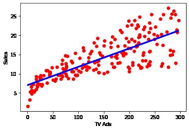
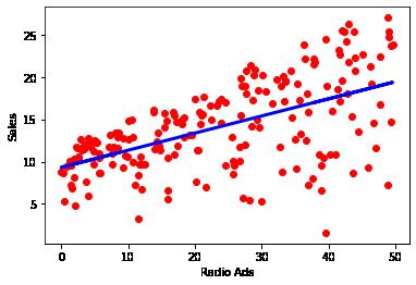
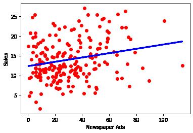
R^2 is highest with TV (followed byt Radio and Newspaper)

We can assume at this point that we can assume the majority the data for TV is explained by the regression model. Radio and Newspaper are less likely to be predicted by the model.

It is also important to point out that this is all based on single varient regression and does little to explain the comination of marketing channels.

Visualizing the best fit line using the regression plot

In [10]: plt.scatter(TV, Sales, color='red') plt.xlabel('TV Ads') plt.ylabel('Sales') plt.plot(TV, tv_model.predict(TV), color='blue', linewidth=3) plt.show()

plt.scatter(Radio, Sales, color='red') plt.xlabel('Radio Ads') plt.ylabel('Sales') plt.plot(Radio, radio_model.predict(Radio), color='blue', linewidth=3) plt.show()

plt.scatter(Newspaper, Sales, color='red') plt.xlabel('Newspaper Ads') plt.ylabel('Sales') plt.plot(Newspaper, newspaper_model.predict(Newspaper), color='blue', linewidth plt.show()

above

Multiple Linear Regression

of

In [11]: mlr_model = linear_model.LinearRegression() mlr_model.fit(Ad_df[['TV', 'Radio', 'Newspaper']], Ad_df['Sales'])

LinearRegression

LinearRegression()

Out[11]: In [12]: Ad_df['Sales_Predicted'] = mlr_model.predict(Ad_df[['TV', 'Radio', 'Newspaper' Ad_df['Error'] = (Ad_df['Sales_Predicted'] Ad_df['Sales'])**2 MSE_MLR = Ad_df['Error'].mean()

In [13]: MSE_MLR Out[13]: In [14]: mlr_model.score(Ad_df[['TV', 'Radio', 'Newspaper']], Ad_df['Sales']) Out[14]:

Observations: The R^2 value for the multiple linear regression comes out to be 89.7% this is a stark improvement over simple LR.

Detailing the model

In [15]: # let us get a more detailed model through statsmodel. import statsmodels.formula.api as smf lm1 = smf.ols(formula= 'Sales ~ TV+Radio+Newspaper', data = Ad_df).fit() lm1

print(lm1.summary()) #Inferential statistics

OLS Regression Results

Dep. Variable: Sales R-squared: 0.8 97 Model: OLS Adj. R-squared: 0.8 96 Method: Least Squares F-statistic: 570 .3 Date: Wed, 19 Oct 2022 Prob (F-statistic): 1.58e96 Time: 12:34:41 Log-Likelihood: -386. 18 No. Observations: 200 AIC: 780 .4

Df Residuals: 196 BIC: 793 .6 Df Model: 3 Covariance Type: nonrobust

coef std err t P>|t| [0.025 0.97 5] Intercept 2.9389 0.312 9.422 0.000 2.324 3.5 54 TV 0.0458 0.001 32.809 0.000 0.043 0.0 49 Radio 0.1885 0.009 21.893 0.000 0.172 0.2 06 Newspaper -0.0010 0.006 -0.177 0.860 -0.013 0.0 11

Omnibus: 60.414 Durbin-Watson: 2.0 84 Prob(Omnibus): 0.000 Jarque-Bera (JB): 151.2 41 Skew: -1.327 Prob(JB): 1.44e33 Kurtosis: 6.332 Cond. No. 45 4.

Notes: [1] Standard Errors assume that the covariance matrix of the errors is corre ctly specified.

In [16]: print("*************Parameters**************") print(lm1.params)

print("*************P-Values**************") print(lm1.pvalues)

print("************Standard Errors***************") print(lm1.bse)

print("*************Confidence Interval**************") print(lm1.conf_int())

print("*************Error Covariance Matrix**************") print(lm1.cov_params())

*************Parameters**************

Intercept 2.938889

TV 0.045765 Radio 0.188530

Newspaper -0.001037 dtype: float64

*************P-Values**************

Intercept 1.267295e-17

TV 1.509960e-81

Radio 1.505339e-54

Newspaper 8.599151e-01 dtype: float64

************Standard Errors***************

Intercept 0.311908 TV 0.001395 Radio 0.008611

Newspaper 0.005871 dtype: float64

*************Confidence Interval************** 0 1

Intercept 2.323762 3.554016 TV 0.043014 0.048516

Radio 0.171547 0.205513 Newspaper -0.012616 0.010541

*************Error Covariance Matrix**************

Intercept TV Radio Newspaper

Intercept 0.097287 -2.657273e-04 -1.115489e-03 -5.910212e-04

TV -0.000266 1.945737e-06 -4.470395e-07 -3.265950e-07

Radio -0.001115 -4.470395e-07 7.415335e-05 -1.780062e-05 Newspaper -0.000591 -3.265950e-07 -1.780062e-05 3.446875e-05

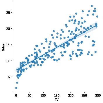
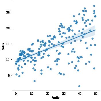
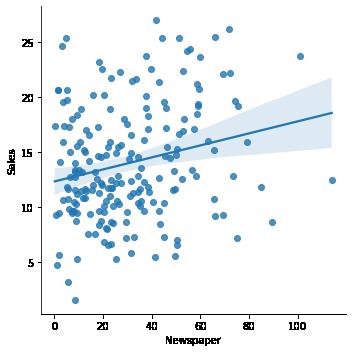
Visualizing the confidence bands in Simple linear regression

In [17]: import seaborn as

'TV', y = 'Sales', data = Ad_df)

'Radio', y = 'Sales', data = Ad_df )

'Newspaper', y = 'Sales', data = Ad_df)

[18]:

[19]:

LVC 2 - Model Evaluation: Cross validation and Bootstrapping

We realize that the newspaper can be omitted from the list of significant features owing to the p-value.

us now run the regression analysis adding a multiplicative feature in it.

let us remove the sales_predicted and the error column generated earlier Ad_df

drop(columns

"Sales_Predicted"],

[20]: # Let us do the modelling with the new feature. import statsmodels.formula.api as

lm2

smf.

= 'Sales ~ TV+Radio+Newspaper+TVandRadio', data = Ad_df lm2

OLS Regression Results

Method: Least Squares F-statistic: 146 6.

Date: Wed, 19 Oct 2022 Prob (F-statistic): 2.92e-1 44 Time: 12:37:10 Log-Likelihood: -270. 04 No. Observations: 200 AIC: 550 .1

Df Residuals: 195 BIC: 566 .6 Df Model: 4 Covariance Type: nonrobust

coef std err t P>|t| [0.025 0.97 5]

Intercept 6.7284 0.253 26.561 0.000 6.229 7.2 28 TV 0.0191 0.002 12.633 0.000 0.016 0.0 22 Radio 0.0280 0.009 3.062 0.003 0.010 0.0 46 Newspaper 0.0014 0.003 0.438 0.662 -0.005 0.0 08 TVandRadio 0.0011 5.26e-05 20.686 0.000 0.001 0.0 01

Omnibus: 126.161 Durbin-Watson: 2.2 16 Prob(Omnibus): 0.000 Jarque-Bera (JB): 1123.4 63

Skew: -2.291 Prob(JB): 1.10e-2 44 Kurtosis: 13.669 Cond. No. 1.84e+ 04

Notes:

[1] Standard Errors assume that the covariance matrix of the errors is corre ctly specified.

The condition number is large, 1.84e+04. This might indicate that there are strong multicollinearity or other numerical problems.

Observations

We see an increase in the R-square here. Now the model must be tested.

Performance assessment, testing and validation

Train, Test, and Validation set

In [21]: from sklearn.model_selection import train_test_split

In [22]: features_base = [i for i in Ad_df.columns if i not in ("Sales" , "TVandRadio" features_added = [i for i in Ad_df.columns if i not in "Sales"] target = 'Sales' train, test = train_test_split(Ad_df, test_size = 0.10, train_size = 0.9)

In [23]: train, validation = train_test_split(train, test_size = 0.2, train_size = 0.80

In [24]: train.shape, validation.shape,test.shape

Out[24]:

We will split data into three sets, one to train the model, one to validate the model performance (not seen during training) and make improvements, and the last to test the model. ((144, 5), (36, 5), (20, 5))

In [25]: # now let us start with the modelling from sklearn.linear_model import LinearRegression

mlr = LinearRegression() mlr.fit(train[features_base], train[target])

print("*********Training set Metrics**************")

print("R-Squared:", mlr.score(train[features_base], train[target])) se_train = (train[target] mlr.predict(train[features_base]))**2 mse_train = se_train.mean() print('MSE: ', mse_train)

print("********Validation set Metrics**************") print("R-Squared:", mlr.score(validation[features_base], validation[target])) se_val = (validation[target] mlr.predict(validation[features_base]))**2 mse_val = se_val.mean() print('MSE: ', mse_val)

*********Training set Metrics************** R-Squared: 0.9098066004061993 MSE: 2.3529856864594056

set Metrics************** R-Squared: 0.8666926059456124 MSE: 4.75733253704616

In [26]: # Can we increase the model performance by adding the new feature?

# We found that to be the case in the analysis above but let's check the same for mlr_added_feature = LinearRegression()

mlr_added_feature.fit(train[features_added], train[target])

print("*********Training set Metrics**************")

print("R-Squared:", mlr_added_feature.score(train[features_added], train[target se_train = (train[target] - mlr_added_feature.predict(train[features_added])) mse_train = se_train.mean() print('MSE: ', mse_train)

print("********Validation set Metrics**************") print("R-Squared:", mlr_added_feature.score(validation[features_added], validation se_val = (validation[target] - mlr_added_feature.predict(validation[features_added mse_val = se_val.mean() print('MSE: ', mse_val)

*********Training set Metrics**************

R-Squared: 0.9776059015819181

MSE: 0.5842222743152014

********Validation set Metrics**************

R-Squared: 0.9354500815069292

MSE: 2.3035888570852756

Observations

We found the R-squared increased as we would expect after adding a feature. Also the error decreased. Let us now fit a regularized model.

Regularization

features_added

['TV', 'Radio', 'Newspaper', 'TVandRadio']

In [28]: from sklearn.linear_model import Ridge from sklearn.linear_model import Lasso

#fitting Ridge with the default features ridge = Ridge() ridge.fit(train[features_added], train[target])

print("*********Training set Metrics**************") print("R-Squared:", ridge.score(train[features_added], train[target])) se_train = (train[target] ridge.predict(train[features_added]))**2 mse_train = se_train.mean() print('MSE: ', mse_train)

print("********Validation set Metrics**************") print("R-Squared:", ridge.score(validation[features_added], validation[target se_val = (validation[target] ridge.predict(validation[features_added]))**2 mse_val = se_val.mean() print('MSE: ', mse_val)

*********Training set Metrics**************

R-Squared: 0.9776059015327091 MSE: 0.5842222755989765

********Validation set Metrics**************

R-Squared: 0.9354506151865334 MSE: 2.303569811695008

In [29]: from sklearn.linear_model import Ridge from sklearn.linear_model import Lasso

#fitting Lasso with the default features lasso = Lasso() lasso.fit(train[features_added], train[target])

print("*********Training set Metrics**************") print("R-Squared:", lasso.score(train[features_added], train[target])) se_train = (train[target] - lasso.predict(train[features_added]))**2 mse_train = se_train.mean() print('MSE: ', mse_train)

print("********Validation set Metrics**************") print("R-Squared:", lasso.score(validation[features_added], validation[target se_val = (validation[target] - lasso.predict(validation[features_added]))**2 mse_val = se_val.mean() print('MSE: ', mse_val)

*********Training set Metrics**************

R-Squared: 0.9767053837296212 MSE: 0.6077151865060982

********Validation set Metrics**************

R-Squared: 0.9363883036797417 MSE: 2.2701065817669406

In [30]: # predict on the unseen data using Ridge

rsq_test = ridge.score(test[features_added], test[target]) se_test = (test[target] ridge.predict(test[features_added]))**2 mse_test = se_test.mean()

print("*****************Test set Metrics******************")

print("Rsquared: ", rsq_test) print("MSE: ", mse_test) print("Intercept is {} and Coefficients are {}".format(ridge.intercept_, ridge

*****************Test set Metrics****************** Rsquared: 0.9681085419848279 MSE: 0.4967054721540549 Intercept is 6.863952092438041 and Coefficients are [ 0.01851559 0.03374944 -0.00117849 0.00106835]

We will now evaluate the performance using the LooCV and KFold methods.

K-Fold and LooCV

In [31]: from sklearn.linear_model import Ridge from sklearn.linear_model import Lasso from sklearn.model_selection import cross_val_score

In [32]: ridgeCV = Ridge() cvs = cross_val_score(ridgeCV, Ad_df[features_added], Ad_df[target], cv = 10 print("Mean Score:") print(cvs.mean(), "\n") print("Confidence Interval:") cvs.mean() cvs.std(), cvs.mean() + cvs.std() # note that the same can be set as LooCV if cv parameter above is set to n, i.e, 200.

Mean Score: 0.9649887636257691

Out[32]:

Confidence Interval: (0.9430473456799694, 0.9869301815715689)

Extra: Statsmodel to fit regularized model

In [33]: # You can also use the statsmodel for the regularization using the below code # import statsmodels.formula.api as smf

# We will use the below code to fit a regularized regression.

# Here, lasso is fit

# lm3 = smf.ols(formula= 'Sales ~ TV+Radio+Newspaper+TVandRadio', data = Ad_df).fit_regularized(method

# print("*************Parameters**************")

# print(lm3.params)

# Here, ridge regularization has been fit

# lm4 = smf.ols(formula= 'Sales ~ TV+Radio+Newspaper+TVandRadio', data = Ad_df).fit_regularized(method

# print("*************Parameters**************")

# print(lm4.params)

Bootstrapping

In [34]: # let us get a more detailed model through statsmodel. import statsmodels.formula.api as smf lm2 = smf.ols(formula= 'Sales ~ TV', data = Ad_df).fit() lm2.params print(lm2.summary()) #Inferential statistics

OLS Regression Results

Dep. Variable: Sales R-squared: 0.6

Model: OLS Adj. R-squared: 0.6

Method: Least Squares F-statistic: 312

Date: Wed, 19 Oct 2022 Prob (F-statistic): 1.47e42 Time: 12:39:39 Log-Likelihood: -519.

Observations: 200 AIC: 104

Residuals: 198 BIC: 104

Model: 1 Covariance Type: nonrobust

coef std err t P>|t| [0.025 0.97

7.0326 0.458 15.360 0.000 6.130 7.9

0.0475 0.003 17.668 0.000 0.042 0.0

Omnibus: 0.531 Durbin-Watson: 1.9

Prob(Omnibus): 0.767 Jarque-Bera (JB): 0.6

Skew: -0.089 Prob(JB): 0.7

Kurtosis: 2.779 Cond. No. 33

that the covariance matrix of the errors is corre ctly

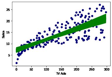
In [43]: #Now, let us calculate the slopes a 1000 times using bootstrapping import statsmodels.formula.api as smf

Slope = [] for i in range(1000): bootstrap_df = Ad_df.sample(n = 200, replace = True ) lm3 = smf.ols(formula= 'Sales ~ TV', data = bootstrap_df).fit() Slope.append(lm3.params.TV)

plt.xlabel('TV Ads') plt.ylabel('Sales') plt.plot(bootstrap_df['TV'], lm3.predict(bootstrap_df['TV']), color='green' plt.scatter(Ad_df['TV'], Ad_df['Sales'], color=(0,0,0.5)) plt.show()

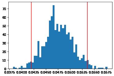
In [38]: # 2.5 and 97.5 percentile for the slopes obtained import numpy as np Slope = np.array(Slope) Sort_Slope = np.sort(Slope)

Slope_limits = np.percentile(Sort_Slope, (2.5, 97.5)) Slope_limits

Out[38]:

array([0.04200087, 0.05356044])

In [39]: # Plotting the slopes and the upper and the lower limits plt.hist(Slope, 50) plt.axvline(Slope_limits[0], color = 'r') plt.axvline(Slope_limits[1], color = 'r')

Out[39]:

<matplotlib.lines.Line2D at 0x7fbe44160850>

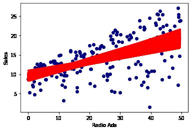
In [45]: #Running a bootstrap analysis for Radio Ads Slope = [] for i in range(1000): bootstrap_df = Ad_df.sample(n = 200, replace = True ) lm4 = smf.ols(formula= 'Sales ~ Radio', data = bootstrap_df).fit() Slope.append(lm4.params.Radio) plt.xlabel('Radio Ads') plt.ylabel('Sales') plt.plot(bootstrap_df['Radio'], lm4.predict(bootstrap_df['Radio']), color= plt.scatter(Ad_df['Radio'], Ad_df['Sales'], color=(0,0,0.5)) plt.show()

In [46]: # 2.5 and 97.5 percentile for the slopes obtained

Slope = np.array(Slope) Sort_Slope = np.sort(Slope)

Slope_limits = np.percentile(Sort_Slope, (2.5, 97.5)) Slope_limits

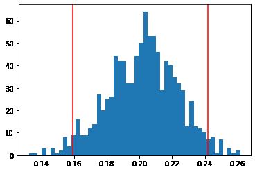
Out[46]:

In [47]: # Plotting the slopes and the upper and the lower limits plt.hist(Slope, 50) plt.axvline(Slope_limits[0], color = 'r') plt.axvline(Slope_limits[1], color = 'r')

Out[47]:

array([0.15927472, 0.24196078]) <matplotlib.lines.Line2D at 0x7fbe28c5e970>

In [ ]:

Observations

Model Accuracy:

We can see from bootstraping both TV and Radio that we can make a fairly accurate prediction on spending to sales.

Both TV and Radio demonstrate a normal distribution

TV and Raido both demonstrate a positive correlation between spending and sales. Newspaer shows no demonstratable predicitive effect.

Recommendation

The combination of Radio and TV provide a marketable differences in sales data. Recommend the continued spending and analysis on current campaigns, and reanalyzing after any changes to campaigns, channels, or timing of addes

Recommend no longer utilizing newspaper ads as a means of direct sales support.

There is no correlation between newspaper spending and sales. note: this recommendation is solely focused on sales parameters, it is not an overview of branding, awareness, nor content effectiveness.