Model Building
Artificial Neural Network (ANN)
Let's create an ANN model sequentially, where we will be adding the layers one after another. Unlike Convolutional Neural Networks, Artificial Neural Networks cannot have images as inputs. We need to pass tabular data to Artificial Neural Networks. Therefore we need to Flatten the images to convert it into 1-D arrays before we feed it to the Fully Connected Layers. Therefore, our first layer in the ANN while working with image data should be a 'Flatten' layer.
In [ ]: ann_model = Sequential()
ann_model.add(Flatten(input_shape = (48, 48, 1)))
# Dense or Fully Connected Layers ann_model.add(Dense(64, kernel_initializer = 'he_normal', activation = 'tanh' ann_model.add(Dense(128, kernel_initializer = 'he_normal', activation = 'tanh' ann_model.add(Dense(256, kernel_initializer = 'he_normal', activation = 'tanh'
# Classifier ann_model.add(Dense(2, activation = 'sigmoid'))
# Adam optimizer with 0.0001 learning rate adam = Adam(0.0001)
# Compiling the model ann_model.compile(loss = 'categorical_crossentropy', optimizer = adam, metrics
In [ ]: # Model summary ann_model.summary()
10/19/22, 10:43 AMBrain_Tumor_Identification_using_MRI_Scans (1) Page 7 of 19file:///Users/jeffreydavis/Desktop/Applied%20Data%20Science/Project…t/Postings%20/Brain_Tumor_Identification_using_MRI_Scans%20(1).html
Model: "sequential" Layer (type) Output Shape Param # ================================================================= flatten (Flatten) (None, 2304) 0 dense (Dense) (None, 64) 147520 dense_1 (Dense) (None, 128) 8320 dense_2 (Dense) (None, 256) 33024 dense_3 (Dense) (None, 2) 514 =================================================================
Total params: 189,378 Trainable params: 189,378 Non-trainable params: 0
In [ ]: # Fitting the model history1 = ann_model.fit(train_set, steps_per_epoch = train_set.n//train_set.batch_size epochs = 10, validation_data = validation_set )
10/19/22, 10:43 AMBrain_Tumor_Identification_using_MRI_Scans (1) Page 8 of 19file:///Users/jeffreydavis/Desktop/Applied%20Data%20Science/Project…t/Postings%20/Brain_Tumor_Identification_using_MRI_Scans%20(1).html
Epoch 1/10
21/21 [==============================] - 7s 305ms/step - loss: 0.7424 - accu racy: 0.5542 - val_loss: 0.6708 - val_accuracy: 0.6076
Epoch 2/10
21/21 [==============================] - 6s 276ms/step - loss: 0.6328 - accu racy: 0.6316 - val_loss: 0.6477 - val_accuracy: 0.6354
Epoch 3/10
21/21 [==============================] - 6s 310ms/step - loss: 0.5995 - accu racy: 0.6660 - val_loss: 0.6074 - val_accuracy: 0.6424
Epoch 4/10
21/21 [==============================] - 6s 286ms/step - loss: 0.5651 - accu racy: 0.7156 - val_loss: 0.5866 - val_accuracy: 0.6771
Epoch 5/10
21/21 [==============================] - 6s 272ms/step - loss: 0.5390 - accu racy: 0.7299 - val_loss: 0.5876 - val_accuracy: 0.6528
Epoch 6/10
21/21 [==============================] - 6s 274ms/step - loss: 0.5292 - accu racy: 0.7457 - val_loss: 0.5321 - val_accuracy: 0.7396
Epoch 7/10
21/21 [==============================] - 6s 293ms/step - loss: 0.5317 - accu racy: 0.7438 - val_loss: 0.5612 - val_accuracy: 0.6944 Epoch 8/10
21/21 [==============================] - 6s 276ms/step - loss: 0.5381 - accu racy: 0.7310 - val_loss: 0.5712 - val_accuracy: 0.7014
Epoch 9/10
21/21 [==============================] - 6s 308ms/step - loss: 0.5246 - accu racy: 0.7446 - val_loss: 0.5393 - val_accuracy: 0.7257 Epoch 10/10
21/21 [==============================] - 6s 304ms/step - loss: 0.5066 - accu racy: 0.7577 - val_loss: 0.5232 - val_accuracy: 0.7257
10/19/22, 10:43 AMBrain_Tumor_Identification_using_MRI_Scans (1) Page 9 of 19file:///Users/jeffreydavis/Desktop/Applied%20Data%20Science/Project…t/Postings%20/Brain_Tumor_Identification_using_MRI_Scans%20(1).html
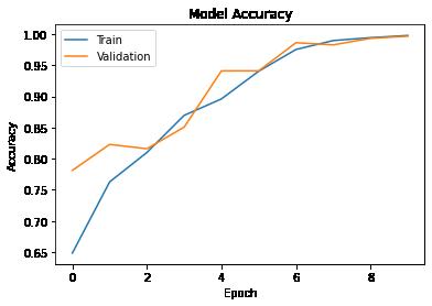
In [ ]: # Plotting training and validation accuracies with the number of epochs on the X-axis plt.plot(history1.history['accuracy']) plt.plot(history1.history['val_accuracy']) plt.title('Model Accuracy') plt.ylabel('Accuracy') plt.xlabel('Epoch') plt.legend(['Train', 'Validation'], loc = 'upper left') plt.show()
Observations:
The validation accuracy showed little fluctuations over 10 epochs. After 10 epochs, the model is giving similar training and validation accuracies of about 77%.
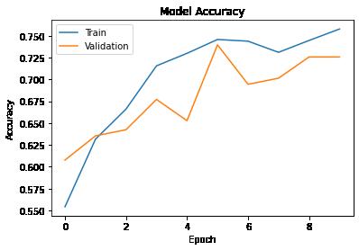
One of the possible reasons can be local spatiality, i.e., since these tumors are present at varying locations within these MRI scans, ANNs wouldn't be able to adjust their weights to detect their presence at a particular location within the image. We can try CNN models to resolve the issue due to local spatiality.
Convolutional Neural Network (CNN)
Let's create a CNN model and see if we get better accuracy than the ANN model.
10/19/22, 10:43 AMBrain_Tumor_Identification_using_MRI_Scans (1) Page 10 of 19file:///Users/jeffreydavis/Desktop/Applied%20Data%20Science/Project…/Postings%20/Brain_Tumor_Identification_using_MRI_Scans%20(1).html
In [ ]: model1 = Sequential()
# First Convolutional block model1.add(Conv2D(16, (3, 3), activation = 'relu', input_shape = (48, 48, 1))) model1.add(MaxPooling2D(2, 2))
# Second Convolutional block model1.add(Conv2D(32, (3, 3), activation = 'relu')) model1.add(MaxPooling2D(2, 2))
# Flattening layer model1.add(Flatten())
# Fully Connected layer model1.add(Dense(128, activation = 'relu'))
# Classifier model1.add(Dense(2, activation = 'sigmoid'))
# Adam optimizer with 0.0001 learning rate adam = Adam(0.0001)
# Compiling the model model1.compile(loss = "categorical_crossentropy", optimizer = adam, metrics
# Model summary model1.summary()
Model: "sequential_1"
Layer (type) Output Shape Param # ================================================================= conv2d (Conv2D) (None, 46, 46, 16) 160 max_pooling2d (MaxPooling2D (None, 23, 23, 16) 0 )
conv2d_1 (Conv2D) (None, 21, 21, 32) 4640 max_pooling2d_1 (MaxPooling (None, 10, 10, 32) 0 2D)
flatten_1 (Flatten) (None, 3200) 0 dense_4 (Dense) (None, 128) 409728 dense_5 (Dense) (None, 2) 258 =================================================================
Total params: 414,786 Trainable params: 414,786 Non-trainable params: 0
10/19/22, 10:43 AMBrain_Tumor_Identification_using_MRI_Scans (1) Page 11 of 19file:///Users/jeffreydavis/Desktop/Applied%20Data%20Science/Project…/Postings%20/Brain_Tumor_Identification_using_MRI_Scans%20(1).html
In [ ]: # Fitting the model history2 = model1.fit(train_set, steps_per_epoch = train_set.n//train_set.batch_size epochs = 10, validation_data = validation_set )
Epoch 1/10
21/21 [==============================] - 10s 446ms/step - loss: 9.8832 - acc uracy: 0.5921 - val_loss: 3.3382 - val_accuracy: 0.7153
Epoch 2/10
21/21 [==============================] - 8s 365ms/step - loss: 2.7900 - accu racy: 0.6978 - val_loss: 1.9653 - val_accuracy: 0.6944
Epoch 3/10
21/21 [==============================] - 8s 367ms/step - loss: 1.7008 - accu racy: 0.7113 - val_loss: 1.6495 - val_accuracy: 0.7153
Epoch 4/10
21/21 [==============================] - 8s 378ms/step - loss: 1.4004 - accu racy: 0.7396 - val_loss: 1.3690 - val_accuracy: 0.7361
Epoch 5/10
21/21 [==============================] - 8s 375ms/step - loss: 1.0041 - accu racy: 0.7864 - val_loss: 1.1683 - val_accuracy: 0.7465 Epoch 6/10
21/21 [==============================] - 8s 367ms/step - loss: 0.8511 - accu racy: 0.7941 - val_loss: 1.0275 - val_accuracy: 0.7639
Epoch 7/10
21/21 [==============================] - 8s 367ms/step - loss: 0.6592 - accu racy: 0.8371 - val_loss: 1.0989 - val_accuracy: 0.7535 Epoch 8/10
21/21 [==============================] - 8s 368ms/step - loss: 0.5038 - accu racy: 0.8618 - val_loss: 0.7727 - val_accuracy: 0.7812 Epoch 9/10
21/21 [==============================] - 8s 358ms/step - loss: 0.5010 - accu racy: 0.8634 - val_loss: 0.7222 - val_accuracy: 0.7812 Epoch 10/10
21/21 [==============================] - 8s 366ms/step - loss: 0.4608 - accu racy: 0.8727 - val_loss: 0.9909 - val_accuracy: 0.8056
#
validation
with the
10/19/22, 10:43 AMBrain_Tumor_Identification_using_MRI_Scans (1) Page 12 of 19file:///Users/jeffreydavis/Desktop/Applied%20Data%20Science/Project…/Postings%20/Brain_Tumor_Identification_using_MRI_Scans%20(1).html
In [ ]:
Plotting training and
accuracies
number of epochs on the X-axis plt.plot(history2.history['accuracy']) plt.plot(history2.history['val_accuracy']) plt.title('Model Accuracy') plt.ylabel('Accuracy') plt.xlabel('Epoch') plt.legend(['Train', 'Validation'], loc = 'upper left') plt.show()
Observations:
Both the train and validation accuracies have improved in comparison to the ANN model. - After 10 epochs, the training accuracy is about 92% and the validation accuracy is about 87%.
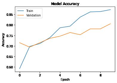
We can further try to increase the model accuracy as even small errors can prove to be very costly in the field of medical research. We observe from the above graph that both train and validation accuracies are displaying an upward trend against the number of epochs. This shows that the model performance can improve further if we increase the model complexity or by training the model for more number of epochs. Below we are trying the former approach.
Increasing the complexity of the CNN Model
Let's see if we can improve the model performance.
10/19/22, 10:43 AMBrain_Tumor_Identification_using_MRI_Scans (1) Page 13 of 19file:///Users/jeffreydavis/Desktop/Applied%20Data%20Science/Project…/Postings%20/Brain_Tumor_Identification_using_MRI_Scans%20(1).html
In [ ]: model2 = Sequential()
# First CNN block model2.add(Conv2D(64, (3, 3), padding = 'same', input_shape = (48, 48, 1))) model2.add(Activation('relu')) model2.add(MaxPooling2D(pool_size = (2, 2)))
# Second CNN block model2.add(Conv2D(128, (5, 5), padding = 'same')) model2.add(Activation('relu')) model2.add(MaxPooling2D(pool_size = (2, 2)))
# Third CNN block model2.add(Conv2D(512, (5, 5), padding = 'same')) model2.add(Activation('relu')) model2.add(MaxPooling2D(pool_size = (2, 2)))
# Fourth CNN block model2.add(Conv2D(512, (5, 5), padding = 'same')) model2.add(Activation('relu')) model2.add(MaxPooling2D(pool_size = (2, 2)))
# Flattening layer model2.add(Flatten())
# First fully connected layer model2.add(Dense(256)) model2.add(Activation('relu'))
# Seconf fully connected layer model2.add(Dense(512)) model2.add(Activation('relu'))
# Classifier model2.add(Dense(2, activation = 'softmax'))
# Adam optimizer with 0.0001 learning rate opt = Adam(learning_rate = 0.0001)
# Compiling the model model2.compile(optimizer = opt, loss = 'categorical_crossentropy', metrics =
# Model summary model2.summary()
10/19/22, 10:43 AMBrain_Tumor_Identification_using_MRI_Scans (1) Page 14 of 19file:///Users/jeffreydavis/Desktop/Applied%20Data%20Science/Project…/Postings%20/Brain_Tumor_Identification_using_MRI_Scans%20(1).html
Model: "sequential_2"
Layer (type) Output Shape Param # =================================================================
conv2d_2 (Conv2D) (None, 48, 48, 64) 640
activation (Activation) (None, 48, 48, 64) 0
max_pooling2d_2 (MaxPooling (None, 24, 24, 64) 0 2D)
conv2d_3 (Conv2D) (None, 24, 24, 128) 204928
activation_1 (Activation) (None, 24, 24, 128) 0
max_pooling2d_3 (MaxPooling (None, 12, 12, 128) 0 2D)
conv2d_4 (Conv2D) (None, 12, 12, 512) 1638912
activation_2 (Activation) (None, 12, 12, 512) 0
max_pooling2d_4 (MaxPooling (None, 6, 6, 512) 0 2D)
conv2d_5 (Conv2D) (None, 6, 6, 512) 6554112 activation_3 (Activation) (None, 6, 6, 512) 0
max_pooling2d_5 (MaxPooling (None, 3, 3, 512) 0 2D)
flatten_2 (Flatten) (None, 4608) 0 dense_6 (Dense) (None, 256) 1179904 activation_4 (Activation) (None, 256) 0 dense_7 (Dense) (None, 512) 131584 activation_5 (Activation) (None, 512) 0 dense_8 (Dense) (None, 2) 1026 =================================================================
Total params: 9,711,106
Trainable params: 9,711,106 Non-trainable params: 0
10/19/22, 10:43 AMBrain_Tumor_Identification_using_MRI_Scans (1) Page 15 of 19file:///Users/jeffreydavis/Desktop/Applied%20Data%20Science/Project…/Postings%20/Brain_Tumor_Identification_using_MRI_Scans%20(1).html
In [ ]: # Fitting the model history3 = model2.fit(train_set, steps_per_epoch=train_set.n//train_set.batch_size epochs = 10, validation_data = validation_set )
Epoch 1/10
21/21 [==============================] - 167s 8s/step - loss: 1.8269 - accur acy: 0.6486 - val_loss: 0.4963 - val_accuracy: 0.7812
Epoch 2/10
21/21 [==============================] - 168s 8s/step - loss: 0.5000 - accur acy: 0.7628 - val_loss: 0.4130 - val_accuracy: 0.8229
Epoch 3/10
21/21 [==============================] - 166s 8s/step - loss: 0.4221 - accur acy: 0.8100 - val_loss: 0.3671 - val_accuracy: 0.8160 Epoch 4/10
21/21 [==============================] - 168s 8s/step - loss: 0.3276 - accur acy: 0.8696 - val_loss: 0.3294 - val_accuracy: 0.8507
Epoch 5/10
21/21 [==============================] - 166s 8s/step - loss: 0.2746 - accur acy: 0.8959 - val_loss: 0.2084 - val_accuracy: 0.9410 Epoch 6/10
21/21 [==============================] - 165s 8s/step - loss: 0.1841 - accur acy: 0.9404 - val_loss: 0.1634 - val_accuracy: 0.9410 Epoch 7/10
21/21 [==============================] - 167s 8s/step - loss: 0.1146 - accur acy: 0.9752 - val_loss: 0.1113 - val_accuracy: 0.9861 Epoch 8/10
21/21 [==============================] - 166s 8s/step - loss: 0.0654 - accur acy: 0.9896 - val_loss: 0.0873 - val_accuracy: 0.9826 Epoch 9/10
21/21 [==============================] - 165s 8s/step - loss: 0.0407 - accur acy: 0.9942 - val_loss: 0.0535 - val_accuracy: 0.9931 Epoch 10/10
21/21 [==============================] - 167s 8s/step - loss: 0.0274 - accur acy: 0.9977 - val_loss: 0.0398 - val_accuracy: 0.9965
# Plotting training
validation
with the number of
10/19/22, 10:43 AMBrain_Tumor_Identification_using_MRI_Scans (1) Page 16 of 19file:///Users/jeffreydavis/Desktop/Applied%20Data%20Science/Project…/Postings%20/Brain_Tumor_Identification_using_MRI_Scans%20(1).html
In [ ]:
and
accuracies
epochs on the X-axis plt.plot(history3.history['accuracy']) plt.plot(history3.history['val_accuracy']) plt.title('Model Accuracy') plt.ylabel('Accuracy') plt.xlabel('Epoch') plt.legend(['Train', 'Validation'], loc = 'upper left') plt.show()
Observations:
The performance of this model is higher in comparison to the performance of previous models. We can see that we have received training and validation accuracies over 99%.
The similar training and validation accuracies show that model is not overfitting the training data.
The possible reason for such improvement is likely the higher number of trainable parameters. As suspected, the earlier models were not complex enough (less number of parameters) to have their weights adjust appropriately to identify the patterns in the images. Hence, we are choosing this model as the final model.
Evaluating Model Performance on the Test data
Observations:
The
is giving the test
of 100%, which is similar to the training and validation
This shows that the final model can
its performance on
10/19/22, 10:43 AMBrain_Tumor_Identification_using_MRI_Scans (1) Page 17 of 19file:///Users/jeffreydavis/Desktop/Applied%20Data%20Science/Project…/Postings%20/Brain_Tumor_Identification_using_MRI_Scans%20(1).html
4/4 [==============================] - 3s 688ms/step - loss: 0.0422 - accura cy: 0.9922 Test_Accuracy:- 0.9921875
model
accuracy
accuracies.
replicate
unseen data. In [ ]: test_images, test_labels = next(test_set) accuracy = model2.evaluate(test_images, test_labels, verbose = 1) print('\n', 'Test_Accuracy:-', accuracy[1])
In [ ]: from sklearn.metrics import classification_report from sklearn.metrics import confusion_matrix pred = model2.predict(test_images) pred = np.argmax(pred, axis = 1) y_true = np.argmax(test_labels, axis = 1)
# Printing the classification report print(classification_report(y_true,
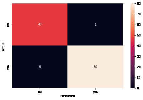
# Plotting the heatmap using confusion matrix cm = confusion_matrix(y_true, pred) plt.figure(figsize = (8, 5)) sns.heatmap(cm, annot = True, fmt = '.0f', xticklabels = ['no', 'yes'], yticklabels plt.ylabel('Actual') plt.xlabel('Predicted') plt.show()
Plotting Classification Matrix precision recall f1-score support
1.00 0.98
0.99
accuracy 0.99
avg
10/19/22, 10:43 AMBrain_Tumor_Identification_using_MRI_Scans (1) Page 18 of 19file:///Users/jeffreydavis/Desktop/Applied%20Data%20Science/Project…/Postings%20/Brain_Tumor_Identification_using_MRI_Scans%20(1).html
0
0.99 48 1
1.00 0.99 80
128 macro
0.99 0.99 0.99 128 weighted avg 0.99 0.99 0.99 128
pred))
Observations:
We can observe from the confusion matrix that 100% of images having a tumor are classified correctly by the model. Classifying a person with no tumor as having tumor is less severe than classifying a person with tumor as having no tumor because the former case can be caught in next stage clinical trials but the later case might go untreated and can prove fatal for the person. But model2 takes care of both these cases.
Hence, we can say the model is reliable to be used in the field of medical research.
Conclusion
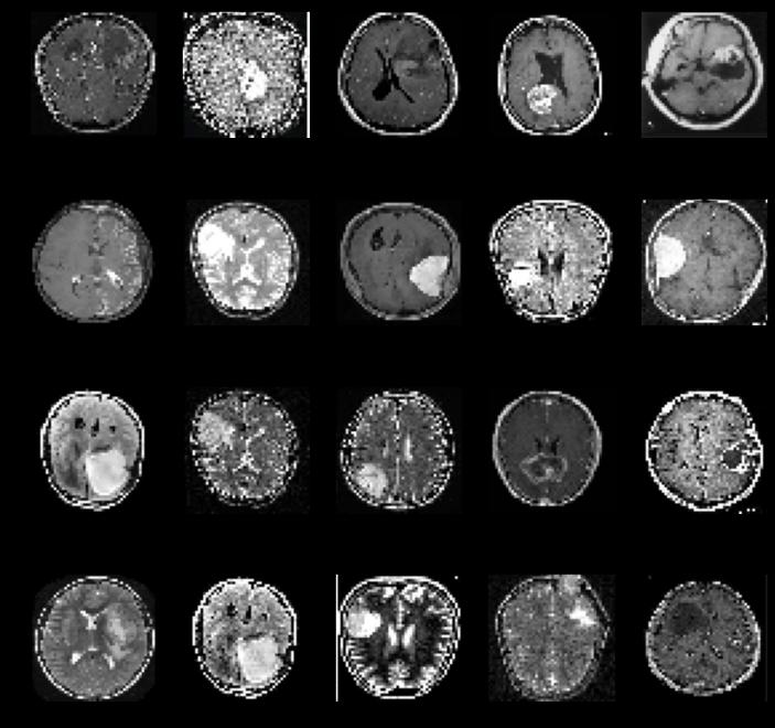
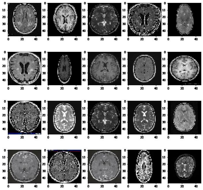
The aim of this problem was to create a Deep Learning model to detect the presence of a brain tumor from MRI scan images. We visualized MRI scans of both types of brains, i.e., having tumor and not having tumor. We saw that brains having tumors had patches of white or gray pixels in either hemisphere of the brain.
The first model was a Fully Connected Neural Network. We observed that the model did not perfom very well on the data at hand. The possible reasons were the lack of ANN's ability to tackle local spatiality as the white or gray patches were present at varying locations.
The second and third models were Convolutional Neural Network architectures. The second model showed good improvement in comparsion to the performance of the first model. However, we chose to build another model, which is more reliable to be used in real world and having very low number of miclassifications. It would be fatal if it were to predict an MRI of an affected brain as being healthy.
Our third model's architecture was slightly more complex. It had many more Convolutional layers, which proved useful. They accurately predicted almost 100% of the MRI scans correctly. Therefore this is the final architecture we propose for this task.
10/19/22, 10:43 AMBrain_Tumor_Identification_using_MRI_Scans (1) Page 19 of 19file:///Users/jeffreydavis/Desktop/Applied%20Data%20Science/Project…/Postings%20/Brain_Tumor_Identification_using_MRI_Scans%20(1).html