ONTARIO OIL AND GAS:
4. Unconventional Resource Potential of Ontario
Phillips, A.1 ; Carter, T.R.2; Fortner, L.4; Clark, J.5; Hamilton, D.2 ; Dorland, M.3; Colquhoun, I.2
1 Clinton-Medina Group Inc., Calgary, AB, 2 Geological consultant, London, ON
3 Geological consultant, Woodstock, ON
4 Ontario Ministry of Natural Resources and Forestry, London, ON
5 Ontario Oil, Gas and Salt Resources Library, London, ON
Introduction
This paper is the fourth of a four-part series. Part 1 summarized the exploration, production and geology of southern Ontario. Part 2 summarized the conventional oil and gas plays of the Cambrian and Ordovician strata of southern Ontario. Part 3 described the conventional oil and gas plays in the Silurian and Devonian strata of southern Ontario. This paper will provide a review of the unconventional resource potential of Ontario.
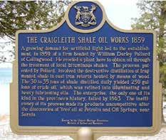
Ontario, or more correctly, Canada West prior to Confederation, was an unconventional oil producer as early as 1859. The Craigleith Oil Shale Works began production in a quarry outside Collingwood and would produce up to 1000 gallons a day of lamp and lubricating oils from 3035 tons of black Ordovician shale in castiron retorts (Dabbs, 2007). The discovery and development of conventional oil production from the Oil Springs and Petrolia Oil Pools in Lambton County, 200 miles to the southwest, proved cheaper and the oil shale operation closed down in 1863.
On the south shore of Lake Erie in Fredonia,
New York, natural gas was being produced from shale 38 years earlier in 1821 (Curtis, 2002). William Hart dug a 27 foot well into the Devonian shales along Canadaway Creek and by 1825 the natural gas was supplying light for two shops, two stores and a grist mill (Harper and Kostelnik, 2007). These two early discoveries proved the existence of unconventional oil and gas production in the area. By the 1860’s cheaper conventional oil and gas production became the dominant product and it would be over 100 years before unconventional resources would come back into the picture.
In late 1982 the Ontario Geological Survey (OGS) initiated the Oil Shale Assessment Project to evaluate the resource potential of Ontario’s Paleozoic black shales. The multi-phase project saw the drilling of core holes in the Province through the 1980’s with additional drilling and testing continuing to the current decade. The Geological Survey of Canada (GSC) has also published a preliminary inventory of Shale Gas possibilities in Canada which included seven organic-rich units in Ontario (Hamblin, 2006). These efforts, in
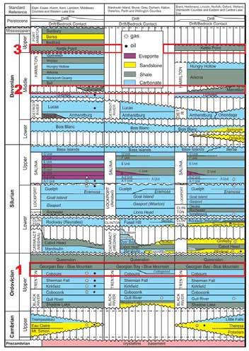
combination with recent shale oil and gas discoveries in surrounding jurisdictions (Pennsylvania , Quebec, Ohio and Michigan) in the Appalachian and Michigan Basins has re-focused attention to Ontario’s unconventional potential. Three of those units in southern Ontario will be examined herein; the organic-rich black shales and mudstones of the Ordovician Collingwood-
(Continued on page 19...) TECHNICAL ARTICLE RESERVOIR ISSUE 11 • DECEMBER 2016 17
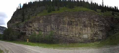
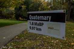
Figure 1. Ontario Heritage Foundation roadside marker near the gate of Craigleith Provincial Park.
Figure 2: Stratigraphic columns of southern Ontario with highlighted organicrich black shale intervals. Modified from Armstrong and Carter (2010).
Blue Mountain (Utica), the Devonian Marcellus, and the Devonian Kettle Point formations (Figure 2).
Ordovician Collingwood-Blue Mountain “Utica”
The black, organic-rich upper Ordovician shales and mudstones that overly the Trenton-Black River carbonates in southwestern Ontario have a complicated nomenclatural history (Armstrong and Carter 2010). The widespread dark grey to black shales seen in oil and gas wells in the subsurface traditionally was called the Collingwood Shale (Sanford, 1961). Those working the outcrop belt and shallow subsurface consider only the transitional shaly limestone section at the top of the Trenton-Black River carbonates to be the Collingwood Member of the Lindsay Formation (Russell and Telford, 1983). The Lindsay Formation is the outcrop equivalent of the Cobourg Formation (Armstrong and Carter, 2010). The thick dark-coloured organic shales above would be the lower part of the Blue Mountain Formation. Recent work by the Ontario Geological Survey (Russell and Telford, 1983; Béland-Otis, 2012) and Sweeney (2014) place these shales into the Rouge River Member of the Blue Mountain Formation. Regardless of which name
is used these shales all form part of the distal portion of the larger “Utica Black Shale Magnafacies” (Lehmann et al, 1995; Hamblin, 2006). These organic-rich strata were deposited under anoxic conditions prior to and during initial deposition of the upper Ordovician siliciclastics in the Appalachian Basin.
The Rouge River organic-rich shales are the lowermost documented facies of the Blue Mountain Formation which in turn is conformably overlain by the Georgian Bay Formation. The two formations are grouped together in the Ontario petroleum well database due to the difficulty of making a consistent formation top pick for the Blue Mountain. The Blue Mountain Formation is dominantly composed of soft, laminated, non-calcareous grey to dark grey shale with only minor interbeds of limestone and siltstone. The proportion of limestone and siltstone beds increases gradually upwards into and within the Georgian Bay Formation. The Georgian Bay-Blue Mountain clastics form a wedge that thickens gradually from northwest to southeast into the Appalachian Basin (Figure 4). Organic-rich facies of the Rouge River Member comprise only the lowermost 2 to 50 metres, also thickening to the southeast. Depth to the top of the Rouge
River ranges from outcrop in the northwest to over 900 metres beneath parts of Lake Erie.
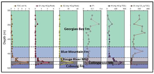
The drilling and testing program conducted by the Ontario Geological Survey to evaluate the resource potential of these black shales has yielded some critical geochemical data (Barker, 1985; Obermajer et al, 1999; Béland-Otis, 2015). These data indicate that some of these black to dark grey mudstones are good to excellent Type II organic-rich source rocks which are thermally mature over a large area in the subsurface of southwestern Ontario (Figure 5). Moving deeper in the basin these organic-rich units thicken.
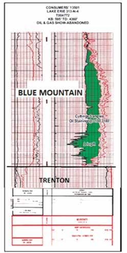
Figure 6 displays an overlay of the sonic and resistivity log of a well drilled in west central Lake Erie in 1978. This Delta Log R technique (Passey et al, 1990) identifies shales with source rock potential. The green highlighted separation between the sonic and resistivity curves is an indicator of good source rock potential. The presence of low velocity kerogen will lower the Δt values on the sonic curve and the higher Rt values on the resistivity curve indicate the presence of generated hydrocarbons in mature source rocks. The wellsite geologist reported oil shows and staining in the
TECHNICAL ARTICLE 18 RESERVOIR ISSUE 11 • DECEMBER 2016
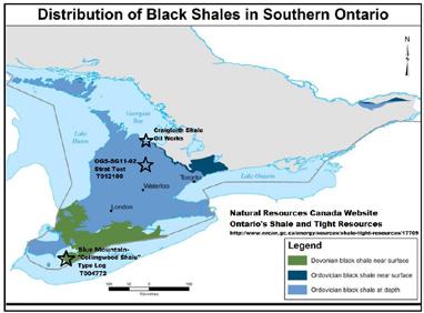
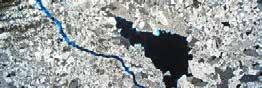
Figure 3: Ordovician black shale distribution (blue) in Southern Ontario. (NRCAN website)
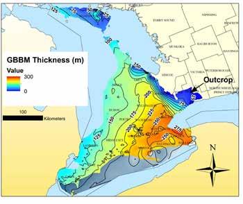
Figure 4. Isopach of the combined Georgian Bay and Blue Mountain (GBBM) formations, showing thickening from northwest to southeast into the Appalachian Basin. Organic-rich facies of the Rouge River Member comprise only the lowermost 2 to 50 metres, also thickening to the southeast.
shale samples through this interval. The shaded cross-over on the Delta Log R plot indicates over 160 feet (48.8m) of source potential in the lowermost Blue Mountain interval. Unfortunately, very few wells in southwestern Ontario have associated resistivity logs. Historic wells in Ontario traditionally did not include wireline logs or only included a GR-Neutron log suite at best, with many wells predating this technology entirely. This makes identification and correlation of these organic-rich units more challenging. Elsewhere in the “Utica” play operators have landed their horizontal wells in the more brittle transitional facies of the upper Trenton Group and steered the horizontal leg up towards the overlying shale contact. In Ohio the Point Pleasant zone is the target. In Encana’s discovery well in Michigan, Petoskey State Pioneer 1-3-HD1, the Collingwood Member at the top of the Trenton was the horizontal landing point and the 5304’ horizontal leg was steered up to the Utica Shale contact (Phillips, 2016).
Resource Potential
In the northeastern United States the Utica Formation is the subject of intensive exploration and evaluation as an unconventional source of natural gas and crude oil. The United States Geological Survey (USGS) has assessed the unconventional oil and natural gas resource potential of the Utica Formation (Kirschbaum et al, 2012) in an area covering parts of Maryland, Ohio, New York, Pennsylvania, Virginia
and West Virginia. They estimate a mean resource volume of 940 million barrels of "technically recoverable" oil and 939 billion cubic feet of associated natural gas within the Utica Shale Oil Assessment Unit (AU) at the 50% probability level, with a range from 590 to 1,386 million barrels at the 95% and 5% probability levels respectively. An additional resource of 37 trillion cubic feet of natural gas and 200 million barrels of natural gas liquids is estimated to occur within the Shale Gas Assessment Unit.
Development of the Utica shale in the United States did not begin until approximately 2010 (Geology.com, 2014). Since that time 1807 horizontal wells have been drilled into the Utica in Ohio alone (http://oilandgas. ohiodnr.gov/shale#SHALE, accessed on Oct.11, 2016). Daily production as of September 12, 2016 totals 3.6 billion cubic feet/day of natural gas and 69,000 barrels/ day of crude oil (Energy Information Administration, 2016).
Total organic carbon content in the Utica Shale Oil AU ranges from 1 to 3%. In Ontario, Obermajer (1999) measured values from 0.74% to 2.69% in the Blue Mountain Formation and up to 7.5% in the Collingwood. In both areas, organic geochemical indicators show the presence of oil-prone Type II organic matter with a thermal maturity in the oil window.
A quantitative resource potential estimate for the Ordovician shales of southern Ontario has not been completed.
of organic-rich shales overlying the Trenton Group. (Phillips, 2014).
Devonian Marcellus
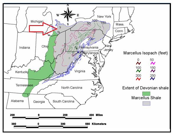
The thick Upper Devonian shale sequence of the Appalachian Basin has seen a lot of interest in recent years. The Marcellus shale gas play is the largest in the United Sates with proved reserves (to end of 2014) of 84.5 Tcf. The Marcellus also had the most reserves (22.1 Tcf) added in 2014 (EIA, 2015). The distal edge of the Marcellus Shale in the Appalachian Basin extends up into southwestern Ontario (Figure 7).
The Ontario Geological Survey included the Marcellus Shale in their resource potential evaluation in the 1980’s (Johnson et al, 1989). Initial mapping indicated that the sub crop edge ran very close to the north shore of Lake Erie and most of the potential
(Continued on page 20...) TECHNICAL ARTICLE RESERVOIR ISSUE 11 • DECEMBER 2016 19
Figure 5: OGS SG11-02, Arthur 4-6-V (T012100) Strat Test. Rock-Eval®6 pyrolysis logs (TOC, S1, S2, PI, HI, OI) from core samples (Béland-Otis, 2015). White-filled dots represent questionable data due to low TOC, S1 and/or S2.
Figure 6: Consumers’ 13501 Lake Erie 313-N-4 (T004772) Δ Log R Plot, sonic-resistivity overlay through the lowermost 200 feet
would therefor be under the lake. This was confirmed with the drilling of five shallow core holes along the north shore of Lake Erie. Only three of the five shallow wells intersected Marcellus Shale. Geochemical analyses were performed on these three shallow cores, core from an industry well at Port Stanley and cuttings samples from several Lake Erie wells targeting deeper Silurian strata. The report concluded that the Marcellus contains a significant thickness of organic-rich Type II/III shale that is marginally mature to mature (Johnson et al, 1989; Hamblin, 2006).
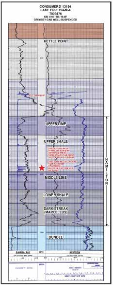
The Devonian black shales have a long history of gas production along the south shore of Lake Erie in New York, Pennsylvania and Ohio. The USGS has grouped them into the Northwestern Ohio Shale and Marcellus Shale Assessment Unit (Milici and Swezey, 2006). The area to the north under Lake Erie is a natural extension to this play. With over 2000 wells drilled in the Canadian waters of Lake Erie a large number have recorded gas shows while drilling through the Devonian shale section. Figure 8 displays the open-hole logs from the Consumers’ 13184 Lake Erie
154-M-4 well drilled in 1972. While drilling at a depth of 584’ (178.0m) the well kicked gas at a rate estimated at 1 MMcf/d (28,320 m3/d). The well was killed with heavier drilling fluid and tested after reaching total depth. The gas rate on the test was reported as 50 Mcf/d (1,416 m3/d) with a shut-in pressure of 235 psig. The caliper log shows washout around the depth where gas was encountered. It is of interest to note the fractured shale unit that produced the gas show is not the lower Marcellus Shale but a more brittle overlying shale unit in the Hamilton Group. Range Resources noted that in their early Marcellus horizontal wells in Washington County, Pennsylvania, those landed in the lower Marcellus section had modest initial production rates averaging only 478 Mcfe/d. Subsequent drilling in the same area during which the horizontal legs were landed higher in the shale section saw significantly higher initial production rates averaging 3,527 Mcfe/d (Zagorski, 2015).
The Marcellus section has yielded a number of gas shows while drilling deeper Silurian gas wells in the central portion of Lake Erie and along the sub crop edge near the north shore of Lake Erie. In a small sampling of 89
used to describe the formations of the Hamilton Group.
wells drilled on Lake Erie around the well shown in Figure 8, 26 wells (29%) had gas shows in the shallow Devonian section as reported by the driller (Phillips, 2014).
Resource Potential
The Marcellus shale gas play is the largest gas field in the United States with 84.5 Tcf in proved reserves at the end of 2014 (U.S Energy Information Administration,
TECHNICAL ARTICLE 20 RESERVOIR ISSUE 11 • DECEMBER 2016
Figure 7: Marcellus Shale Isopach Map (Milici, 2005).The red arrow indicates the extension of the shales into southern Ontario.
Figure 8. Open-hole logs Consumers’ 13184, Lake Erie 154-M-4, showing the Devonian shale section from Kettle Point at 367 feet to top of Dundee Formation limestone at 689 feet. Driller terminology has been
2015) and a mean undiscovered natural gas liquids resource of 3.4 billion barrels (Coleman et al, 2011). Annual production in 2014 totaled 4.9 Tcf of natural gas. The Marcellus play underlies an area of over 72,000 square miles, occurring in a continuous accumulation encompassing most of Pennsylvania, West Virginia, Ohio, and New York, and parts of Maryland, and Virginia. Depths to the Marcellus vary from outcrop to nearly 11,000 feet (3350 metres), with most production occurring where the formation is 2,000 to 6,000 feet below sea level (http://www.eia.gov/todayinenergy/ detail.php?id=20612). Thickness varies from less than 50 feet to 300 feet (15-90 m.) in most of the productive area, reaching even greater thicknesses feet in New York. Production is derived almost exclusively from horizontal wells completed with multi-stage high volume hydrofracture treatments. Hydraulic fracturing has been banned in New York State.
There have been no horizontal wells drilled in the Marcellus in Ontario and there is no production from this formation. No quantitative resource assessment has been completed.
Devonian Kettle Point
The Upper Devonian Kettle Point
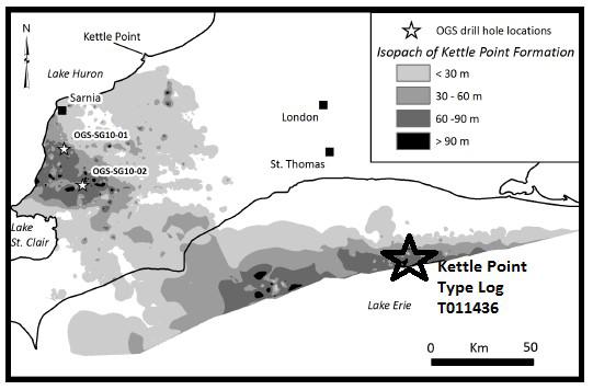
Formation overlies the Hamilton Group (which includes the Marcellus Shale) and is preserved through the central portion of southwestern Ontario in the Chatham Sag (Figure 9), underlying an area of over 4,000 square kilometres.
Typically, the Kettle Point Formation is overlain by Quaternary sediments, except for a small area south of Sarnia where Port Lambton Group shales and siltstones overlie the Kettle Point Formation. It is equivalent to the productive Antrim shale in Michigan and the Ohio shales in Ohio, Pennsylvania and New York (Russell, 1985). The Kettle Point succession of black organicrich shales and grey-green organic-lean shales can exceed 100 metres thickness, but the preserved thickness is generally much less, averaging about 30 metres. The black shales within the sequence exhibit the highest organic content up to 15.1 wt.%, with thermal maturity data indicating these shales to be immature to marginally mature (Barker, 1985; Obermajer et al, 1997).
Drilled in the summer of 2006 eleven wireline recoverable cores (105.50164.65m) were cut in the Kettle Point Shale and three wireline recoverable cores (186.50-209.00m) were cut in the Marcellus Shale interval. Total organic carbon values
in the Kettle Point were measured at 6.08 and 12.87 wt. % (Phillips, 2014). These values fall in line with those obtained from the Ontario Geological Survey onshore Ontario wells (Béland-Otis, 2013).
Early reports from the Geological Survey of Canada refer to the common seepage of natural gas from the thick sand and gravel deposits that overlie the Kettle Point Formation. Water well records commonly record the occurrence of natural gas in the groundwater in the same area (Singer et al., 1997, 2003) and petroleum well records document gas shows in the upper few metres of the Kettle Point (Carter et al, 2008). Many domestic water wells in areas underlain by the Kettle Point black shales must be vented outdoors to prevent methane from entering residences and farm buildings.
The Ontario Geological Survey drilled and cored 2 boreholes through the full thickness of the Kettle Point formation to collect core and gas samples (BélandOtis, 2013). Drill core samples from the boreholes were analysed for gas content, gas composition, isotopic composition of methane, total organic carbon, oil, gas and water saturation, permeability, porosity, mineralogy, adsorption isotherms and rock mechanics. Both thermogenic and biogenic gas were identified. The stratigraphicallyequivalent Antrim Shale Play to the west in central Michigan also includes a significant component of biogenic gas (Martini et al, 2003).
The open hole logs from the Talisman Central Lake Erie 157-V-4d (T011436) in Figure 10 illustrate the Devonian Kettle Point and Marcellus Shale section.
Resource Potential
The Antrim Shale in Michigan has been developed by over 9000 wells, with cumulative production of 2.5 trillion cubic feet of natural gas to the end of 2006 (Goodman and Maness, 2008), and exceeding 3 Tcf of natural gas to date. Annual production at the end of 2006 totalled 140 billion cubic feet which declined to 95 billion cubic feet by 2014. Well depths range from 150 to 600 metres. Many wells have been on production for more than 30 years.
(Continued on page 22...) TECHNICAL ARTICLE RESERVOIR ISSUE 11 • DECEMBER 2016 21
Figure 9. Isopach map of the Kettle Point Formation (Béland Otis, 2013).Well T003476 in Fig.8 is located 20 km east of well T011436.
A significant proportion of the natural gas in the Antrim has been produced by in situ microbial methanogenesis (Martini et al, 2003) of organic carbon. The identification of biogenic gas in the Kettle Point Formation suggests that the same play type may occur in southern Ontario.
No quantitative resource assessment of the Kettle Point Formation in southern Ontario has been completed.
Summary
To date only a handful of vertical wells have cored and tested the Ordovician and Devonian shales and mudstones in Ontario. Most of these data have confirmed hydrocarbon potential within these units. No horizontal wells have been attempted to test the resource potential of shales in Ontario. The shallow depths and proximity to large urban centres may present some unique challenges for future development, as well as opportunities.
References
Armstrong, D.K., and Carter, T.R., 2010. The subsurface Paleozoic stratigraphy of southern Ontario; Ontario Geological Survey, Special Volume 7, 301p.
Barker, J.F., 1985. Geochemical Analysis of Ontario Oil Shales; Ontario Geological Survey, Open File Report 5568, 77p.
Béland Otis, C., 2012. Shale Gas Potential for the Ordovician Shale Succession of Southern Ontario; Oral Presentation at the AAPG Eastern Section Meeting, Cleveland, Ohio, USA. Search and Discovery Article #50730 (2012).
Béland (Otis, C., 2013. Gas Assessment of the Devonian Kettle Point Formation; Ontario Geological Survey Open File Report 6279, 63p.
Béland Otis, C., 2015. Upper Ordovician Organic-Rich Mudstones of Southern Ontario: Drilling Project Results; Ontario Geological Survey Open File Report 6312, 59p.
Carter, T.R., Fortner, L., and Béland Otis, C., 2008. Shale Gas Opportunities in Southern Ontario – an Update. Oral Presentation at the 48th Annual OPI Conference and Trade Show, Sarnia, Ontario, Canada, November 11-13, 2008.
Coleman, J.L., Milici, R.C., Cook, T.A., Charpentier, R.R., Kirschbaum, M., Klett, T.R., Pollastro, R.M., and Schenk, C.J., 2011. Assessment of undiscovered oil and gas resources of the Devonian Marcellus Shale of the Appalachian Basin Province, 2011; United States Geological Survey, Fact Sheet 2011-3092, 2 p. available at http://pubs. usgs.gov/fs/2011/3092/.
Curtis, J.B., 2002. Fractured shale-gas systems; Bulletin of American Association of Petroleum Geologists, v. 86, No. 11 (November 2002), p. 1921-1938.
Dabbs, F., 2007. Craigleith Oil Shale Works, Ontario; Petroleum History Society Archives, Volume XVIII, Number 2.
Geology.com, 2014. Utica Shale - The natural gas giant below the Marcellus, accessed July 30, 2014 at http://geology. com/articles/utica-shale/.
Hamblin, A.P., 2006. The “Shale Gas” concept in Canada: a preliminary inventory of possibilities; Geological Survey of Canada, Open File Report 5384, 103p.
Harper, J. A., and Kostelnik, J., 2007. The Marcellus Shale Play in Pennsylvania Part 1: A Historical Overview, Pennsylvania Department of Conservation and Natural Resources, Pennsylvania Geological Survey, Marcellus Shale Play, Pennsylvania DCNR webpage
Johnson, M.D., Telford, P.G., Macauley, G., and Barker, J.F., 1989. Stratigraphy and oil shale resource potential of the Middle Devonian Marcellus Formation, southwestern Ontario; Ontario Geological Survey, Open File report 5716, 149p.
Kirschbaum, M.A., Schenk, C.J., Cook, T.A., Ryder, R.T., Charpentier, R.R., Klett, T.R., Gaswirth, S.B., Tennyson, M.E., and Whidden, K.J., 2012. Assessment of undiscovered oil and gas resources of the Ordovician Utica Shale of the Appalachian Basin Province, 2012: U.S. Geological Survey Fact Sheet 2012–3116, 6 p.
Lehmann, D., Brett, C.E., Cole, R. and Baird, G., 1995. Distal sedimentation in a peripheral foreland basin: Ordovician black shales and associated flysch of the western Taconic foreland, New York State and Ontario; Geological Society of America Bulletin, v. 107, p.708-724.
Martini, A.M., Walter, L.M, Ku, T.C.W., Budai, J.M., McIntosh, C., and Schoell, M., 2003. Microbial production and modification of gases in sedimentary basins: A geochemical case study from a Devonian shale gas play, Michigan
TECHNICAL ARTICLE 22 RESERVOIR ISSUE 11 • DECEMBER 2016
Figure 10. Kettle Point type well (Phillips, 2014), showing Kettle Point Formation from 82.5 metres to 156.2 metres. Driller terminology has been used to describe the formations of the underlying Hamilton Group.
basin, Bulletin of American Association of Petroleum Geologists, v. 87, No. 8 (August 2003), p. 1355-1375.
Milici, R.C., 2005. Assessment of Undiscovered Natural Gas Resources in Devonian Black Shales, Appalachian Basin, Eastern U.S.A.; U.S. Geological Survey Open File Report 2005-1268, 31p.
Milici, R.C., and Swezey, C.S., 2006. Assessment of Appalachian Basin Oil and Gas Resources: Devonian Shale-Middle and Upper Paleozoic Total Petroleum System; U.S. Geological Survey Open File Report 2006-1237, 70p.
Obermajer, M., Fowler, M.G, and Snowdon, L.R., 1999. Depositional Environment and Oil Generation in Ordovician Source Rocks from Southwestern Ontario, Canada: Organic Geochemical and Petrological Approach; Bulletin of American Association of Petroleum Geologists, v. 83, No. 9 (September 1999), p. 1426-1453.
Passey, Q.R., Creaney, S., Kulla, J.B., Moretti, F.J., and Stroud, J.D., 1990. A Practical Model for Organic Richness for Porosity and Resistivity Logs; Bulletin of American Association of Petroleum Geologists, v. 74, No. 12 (December 1990), p. 1777-1794.
Phillips, A.R., 2014. Devonian and Ordovician Shale Correlations Under Lake Erie, Bridging the Gap; Oral Presentation at the AAPG Eastern Section Meeting, London, Ontario, Canada, September 2730, 2014.
Phillips, A.R., 2016. North America’s First Oil Shale Play, Ordovician Collingwood (Utica) Shale in Southwestern Ontario; Core Workshop, 54th Annual OPI Conference and Trade Show, London, Ontario, Canada, May 4, 2016, 47p.
Russell, D.J., 1985. Depositional Analysis Of A Black Shale Using Gamma-Ray Stratigraphy: The Upper Devonian Kettle Point Formation Of Ontario; Bulletin of Canadian Petroleum Geology, v. 33, No. 2 (June, 1985), p. 236-253.
Russell, D.J. and Telford, P.G., 1983. Revisions to the stratigraphy of the Upper Ordovician Collingwood Beds of Ontario –A potential oil shale; Canadian Journal of Earth Sciences, v.20, p.1780-1790.
Sanford, B.V., 1961. Subsurface Stratigraphy of Ordovician Rocks in Southwestern Ontario; Geological Survey of Canada, Paper 60-26. 54p.
Sweeney, S.N., 2014. Allostratigraphy of the Upper Ordovician Blue Mountain Formation, southwestern Ontario, Canada. MSc thesis, University of Western Ontario, electronic thesis and dissertation repository, Paper 2555, 301 p., http://ir.lib. uwo.ca/etd/2555/
United States Energy Information Administration, 2016. Drilling productivity report release date September 12, 2016 accessed Oct.11, 2016 at www.eia.gov/ petroleum/drilling/#tabs-summary-2.
United States Energy Information Administration, 2015. U.S. Crude Oil and Natural Gas Proved Reserves, 2014; U.S. Energy Information Administration Report. 49p.
https://www.eia.gov/state/print. cfm?sid=MI
Zagorski, B., 2015. Marcellus ShaleGeological Considerations for an Evolving North American Liguids-Rich Play; Oral Presentation at AAPG DPA Playmaker Fourm, “From Prospect to Discovery”, January 24, 2013, Houston, Texas. Search and Discovery Article #110183 (2015).
TECHNICAL ARTICLE RESERVOIR ISSUE 11 • DECEMBER 2016 23


Wednesday September 20, 2017


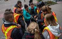
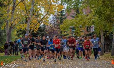
24 RESERVOIR ISSUE 11 • DECEMBER 2016 THANK-YOU to the all the participants, sponsors and volunteers
the 28th Annual 10k & 5k Road Race and Fun Run! Top 10KM Top 5KM CSPG Female Holly Ratzlaff 0:42:29.5 CSPG Female Tina Donkers 0:26:48.1 CSPG Male Darren Lazaruk 0:40:43.2 CSPG Male Cameron Demmans 0:19:37.2 CSEG Female Shannon Bjarnsason 0:48:59.5 CSEG Female Jocelyn Frankow 0:27:09.6 CSEG Male Darren Hinks 0:41:17.9 CSEG Male Franck Delbecq 0:18:17.0 CAPL Male Sean McLeod 0:42:59.2 Ken Buckley 0:29:01.2 CAPL Male
of
29th Annual Road Race and Fun Run
The Geology of Wine Tasting
Jon Noad, Sedimental Services
Iam sure that there are many geologists who take a keen interest in wine, and not just in drinking it. Explaining the vast diversity of quality, flavours and aromas is no simple task, and what fascinates me is the relative role of the geology, and the associated soils, in determining which vineyards are winners and losers. Many factors will influence the character of the wine, generally summarized under the French term “terroir”.
What is terroir? The term was developed in France in the late 1960s to encompass the totality of the setting, or the “sense of place”, in which the grapes grow. The term has some almost mystical connotations, but includes the climate and weather, the soils and geology, as well as the slope and aspect (direction in which the slope faces). All of these characteristics are thought to have a significant influence on the flavour of whichever grape species has been chosen for cultivation. After harvesting, the processes used by the grower to transform the grapes into wine will have a key influence on the flavour, and the wine will also change character through maturation after bottling.
The impact of geology and soil
So how much influence does the geology have on the final product, compared to the climate? This topic was examined by James E. Wilson (a retired petroleum geologist) in 1998, in his book “The role of Geology, Climate and Culture in the making of French Wines”, and revisited in a series of articles by Simon Haynes of Calgary. Obviously a significant area of land is affected by broadly similar weather patterns, so the disparity in the quality of wines produced from adjacent vineyards, often at the same elevation and slope orientation, cannot be explained by differences in climate alone. This shifts the focus onto the geology and soil as key influences on the grape character.
The chemical analysis of wines confirms that the associated flavours are due to nutrient elements (typically metallic
cations) and only distantly related to geological minerals, which are complex crystalline compounds (Maltman 2013). Hence the chemical composition of the rocks will not directly influence the grapes, particularly as the actual concentrations of mineral elements are typically miniscule, in part because they are relatively insoluble. Almost all minerals are also flavourless, with the exception of halite, and our mouths are unable to taste them. They are also lacking in aroma, with a few unpleasant exceptions, such as sulphur. So it is clearly not the mineral composition of the rocks that affect the taste, but must be something else.
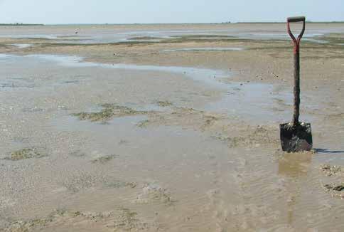
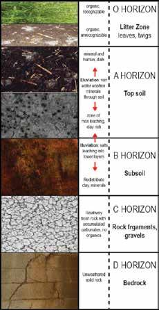
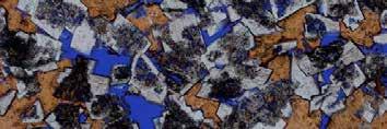
Geology directly affects the soil, in that soils form from the breakdown of bedrocks over time (Figure 1). It is suggested that a typical soil forms at around an inch every thousand years. Immature soils are not layered, and are little more than gravels overlying bedrock, but mature soils may be stratified with surficial organic debris, topsoil and gravelly subsoil. Once the soil has formed it will affect the vines in two significant ways: firstly the level of nutrients in the soil will nourish the vines to a certain degree. More importantly, the soil and the underlying weathered bedrock will act as a conduit, inhibiting or enhancing the flow of groundwater, as well as potentially acting as a reservoir for water to replenish the vine through its root system.
Grapes respond to both feast and famine; hardship in the form of arid soils will usually lead to smaller grapes with more concentrated flavours. However yields will consequentially be much lower in such environments. The presence of water, stored in fractures in the bedrock near the surface, may provide vines with a longer growing season. However in areas of thicker, porous soils, the roots of vines may have to extend more than 50 metres into the subsurface in the search for water, meaning that a great deal of photosynthetic energy may be expended. This may in turn adversely affect the quality of the grapes on the vine. In very fertile, damp soils, the grapes may become “flabby”, with softer flesh and more dilute
flavours.
Finally geology has a very obvious impact on the topography. Igneous and metamorphic rocks may weather to very rugged terrains, while softer (usually younger) sediments may lead to very flat, poorly drained areas, where vines will grow less successfully. The geology will also affect the degree and aspect of the slope. Very steep slopes drain effectively, but may lead to arid environments, with too little available water for the vines to suck up. Hence there are several ways in which the geology can impact eventual wine quality, and the right balance between adversity and plenty is needed to create the perfect wine.
RESERVOIR ISSUE 11 • DECEMBER 2016 25 SOCIETY ARTICLE
Figure 1. Typical soil profile (after a figure by Owais Khattak).

A flavourful case study
Working with a sommelier from the COOP, we recently put together a wine tasting event that explored a variety of terroirs, and the potential impact of the geology on the various wines offered for sampling. A mixed audience of geologists and wine fanciers were in attendance to evaluate the relative contributions of climate and geology. Below I have selected some of the chosen wines, in order to highlight the geological contribution to their character (Figure 2).
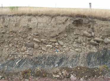
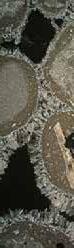
First up was a Sauvignon blanc from the Marlborough region of New Zealand. These dry, white wines are renowned for their extremely fruity flavours, which may come close to overpowering the wine. Most of the vineyards are located on older river terraces, which may feature a fine grained, river borne (silts and muds) or windblown (loess) component, in addition to poorly sorted river pebbles. The river gravels are often only a couple of metres thick, underlain by metamorphosed bedrock (Figure 3), but may reach 30 m in thickness, when they will require drip irrigation. These cannot really be described as soils.
This geology is little different to the geology of the Loire Valley, where some of the world’s great sauvignon blancs (Sancerre, for example) are grown. However in France they are dry and “flinty” (a term relating to the acid hints in the wine only), rather than exceptionally fruity in character. Considerable scientific study of the Antipodean white wines (how would
you fancy a PhD. looking at the geology of wine?) indicates that the reason for this fruitiness is the presence of thiols, chemicals that impart the classic kiwi and peach notes to the wine. The thiol concentrations are enhanced by machine harvesting (which presumably bruises the grapes), by the presence of unique yeasts (thought to relate to the very high UV levels, around 30% above the norm) and by higher than usual temperature fluctuations. Hence the geology apparently plays less of a role than climate in determining the character of this wine, acting mainly as a conduit.
A fascinating comparison between a South African Chardonnay from Stellenbosch and a Chablis from Burgundy demonstrated that these very similar grapes produced more acidic notes when planted on French gravel scree slopes derived from weathering of Jurassic limestones, with water trapped by Kimmeridgian clays. In contrast the South African soils have been forming for around 65 million years, and are very depleted in minerals and nutrients. Lime and phosphate have to be added to the acid, granitic soils, and the chardonnay wine is softer and more “middle of the road” as a result of the additives.
Rosés are Red
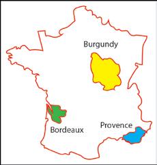
Provence is considered as the spiritual home of Rosé wines, and exhibits a striking spectrum of these wines ranging from pale pinks with a delicate taste, through to bold, almost ruby wines with a strong berry component. The reason is almost certainly
26 RESERVOIR ISSUE 11 • DECEMBER 2016 SOCIETY ARTICLE
Figure 2.The range of wines selected for the Geology of Wine tasting (part 1). Figure 3. Soil profile showing gravel development, Marlborough region, New Zealand (www.glug.com.au).
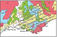
Figure 4. Geological map of Provence (shaded).
France Wine Locations
the contrast between the arid, Cretaceous limestone soils, and the weathering products of the ancient crystalline massifs to the East (Figure 4). The grapes utilized include tight bunhes of the tiny, strongly flavoured cinsault, which can be eaten from the vine.
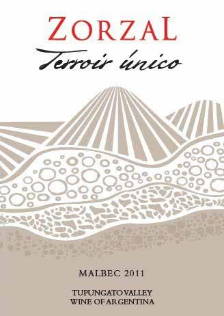
Turning to the reds, the Malbecs of Argentina have a huge range in quality and taste. This relates directly to the geology, with a mix of outcropping volcanics and limestones, as well as alluvial gravels and silts (Figure 5). Such a diverse “rock garden” may be encountered at a single vineyard. The winemaker typically has to dig a series of pits across his property in order to evaluate where to plant the vines, and blending is employed to smooth out the localized vagaries in quality.
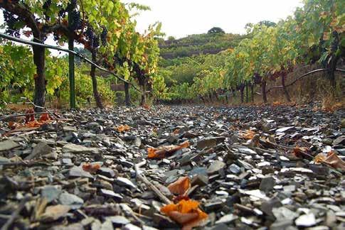
Next we chose the Priorat region of NE Spain for its unique terroir. The geology is striking, with very rugged topography and exceptionally stoney soils (Figure 6). Shards of dark grey, Carboniferous slate spall from the underlying bedrock, and form a poor soil termed as “llicorella” in the Catalan language. Associated mica in the top 50 cm, eroded from volcanic rocks, traps water beneath it. The yields are very low, with the Garnacha vines basically growing on weathered bedrock, their roots penetrating deeply in their search for water, but the
flavours are intense in what is one of the country’s best and most expensive wines.
Classic wines on display
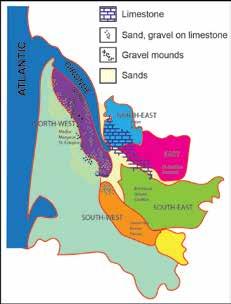
Bordeaux is justifiably one of the world’s most famous wine growing regions. The landscape and geology are very variable, meaning that different wines flourish in different settings (Figure 7). Vineyards southwest of the Gironde River are planted on poorly sorted, glacial derived, river terraces, the best wines (like Margaux and Medoc) harvested from terraces around 700,000 to a million years in age. The other side of the river includes St. Emilion, grown on Tertiary limestones, and Pomerol, also grown on river terrace gravels. The gravels host small, dark grapes, which are stressed and therefore rich in flavour, while the limestone related wines are softer and easy drinking.
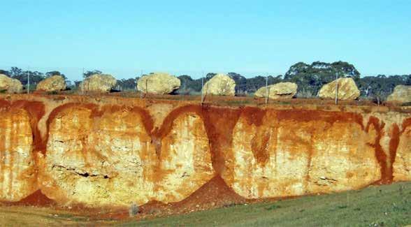
Our final wine region is located around the town of Coonawarra, some 400 km south of Adelaide in South Australia. This area produces one of the world’s great Cabernet sauvignon wines, grown on terra rosa soils (Figure 8). These soils comprise insoluble red clays produced by the karstic weathering of limestone, colored by iron oxides preserved above the water table. The clay allows surprisingly good drainage, in an area with a maritime climate similar to the Bordeaux region. The wines are full of
plum and blackcurrant notes.
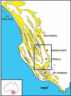
The terroir covers a narrow belt around 20 km long and only 2 km wide, located on a limestone ridge, located between two of a series of subparallel dune fields (Figure 9). The Coonawarra red soils formed just to the west of the beach rocks, and overlie rocks deposited on the edge of a lagoon. Using oil exploration methodology, one might hope to use the sweet spot at Coonawarra
RESERVOIR ISSUE 11 • DECEMBER 2016 27
SOCIETY ARTICLE
Figure 5. Geological Malbec wine label from Argentina.
Figure 6. Llicorella slate soil and vines, Priorat (from catalanwine365.wordpress.com).
Figure 7. Map of Bordeaux wine region showing the soil and wine distribution.
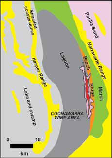
as a potential analogue for other terra rosa deposits between other dune fields (Figure 10). However this is a classic example of where a simple exploration play seems to work only once, although work continues to try and identify other areas where similarly spectacular wines could be grown.
It’s all in the plumbing
In conclusion, geology and soils are critical in helping to develop flavours of grapes on the vine. However it is not the associated minerals that lead to the flavours, but rather the porosity and permeability of the soils. The soils act like a hydroponic tank, water typically running through a framework of gravels beneath the surface,
with an underlying storage medium made up of fractured bedrock. The geology also affects the nutrient levels in the soil, which may help or hinder vine growth, as well as controlling the topography of the vineyard. However when someone starts telling you that they can “taste the minerality”, you will know better!
Note:
The CSPG is planning on hosting a Geology of Wine Tasting early in 2017. This is your chance to learn about the impact of terroir and “vini-geology” on flavour, while you taste some impressive vintages. Watch this space for further details!
28 RESERVOIR ISSUE 11 • DECEMBER 2016 SOCIETY ARTICLE
Figure 8. Striking terra rosa soils overlying limestone at Coonawarra (www.glug.com.au).
Figure 9. Geological sketch map of Coonawarra wine region (www.glug.com.au).
Figure 10. Map of Pleistocene dunes around Coonawarra (after http://sahistoryhub.com.au)
2016 Gussow Geoscience Conference: Clastic
Sedimentology: New Ideas and Applications
October 11th to 13th, 2016, Banff, Alberta
Jon Noad, Conference Chair

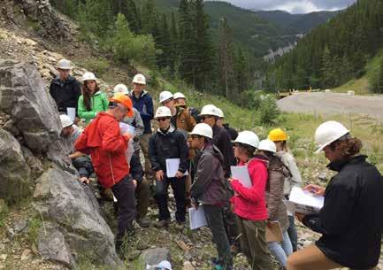
This year’s conference was held at the Banff Centre, and was, without any doubt, a resounding success. The conference co-chairs received universally positive feedback from all those who attended, both in terms of the venue and the outstanding quality of the talks. The hard work of the five conference co-chairs (Noad, Jablonski, Tye, Ranger and MacEachern), coupled with the outstanding efforts of the session chairs (Miall, Hasiotis, Dashtgard, Gingras, Fielding, Bann, Hubbard, Arnott, Slatt, and Plint) ensured a strong technical program filled with engaging presentations and poster displays.
The conference was split into five sessions, which followed a “source to sink” pattern, beginning with terrestrial (fluvial), passing through estuarine (paralic) and shoreface systems into deep water deposits, and finishing with a mud session. Each session commenced with an excellent introductory overview from the session chairs, all of whom stressed the rapid progress in their subdivision of the field of clastic sedimentology.
Talks in the terrestrial session examined existing models for alluvial facies (Fielding), as well as questioning the interpretation and abundance of braided channels deposits in the fossil record (Blum). The braided to meandering transition was also examined (Noad), and these fluvial
themes generated animated discussion, which was great to see at the conference. We investigated preservation and geological time (Miall), and then looked at quantitative facies models (Colombera). The session concluded with a whirlwind tour of terrestrial trace fossils (Hasiotis) and their significance. Particularly striking were the Triassic crayfish beds of Utah.
After an evening where most of the attendees sampled the food and beverages of Banff, (as well as discovering a handy short cut back to the Banff Centre that skirted the cemetery), the following day kicked off with the paralic-estuarine session. We were treated to several discourses on facies models for transitions from fresh water fluvial channels, through estuaries and to the shoreline, with cosmopolitan examples from the Gironde of France (Fenies), Willapa Bay (Gingras) and the Sittaung River of Myanmar (Choi). Talks zoomed
in to look at the morphology of tidal bars (Schoengut) and distributary channels (La Croix), before a visit to some stunning riverside outcrops of the McMurray Formation (Jablonski) demonstrated how Lidar style data can be used in numerical analyses.
After lunch we moved to the fully marine shoreface, with three of the talks looking at deltaic deposits of the Wilrich (Bann), Viking (MacEachern) and the modern Fraser River Delta (Ayranci). Of particular interest was the way that trace fossil data was used to delineate subtleties of depositional settings. A sequence stratigraphic framework was employed to demonstrate both falling stage conditions and delta asymmetry in the Viking. A subsequent tidal facies talk showed facies criteria for identifying tidal signatures in shoreface settings (Dashtgard). We also looked at Permian deposits of Australia
RESERVOIR ISSUE 11 • DECEMBER 2016 29
SOCIETY ARTICLE
Photo by Jon Noad
CORPORATE SUPPORTERS
I H S Markitt
Birchcliff Energy Ltd.
Pro Geo Consultants
RPS Energy Canada Ltd.
Bannatyne Wealth Advisory Group
Canadian Global Exploration Forum
CMC Research Institutes, Inc.
Encana
EV Cam Canada Inc.
Halliburton
RIGSAT Communications
RS Energy Group
Schlumberger Canada Limited
Cabra Consulting Ltd.
Pulse Seismic Inc
McDaniel & Associates Consultants Ltd.
CAPL
ConocoPhillips
Earth Signal Processing Ltd.
Mount Royal University
Valeura Energy
YaleCanada
Compass Directional Services
Integrated Sustainability Consultants Ltd.
TAQA North Ltd.
Navigator Resource Consulting
Synterra Technologies
Baker Hughes Calgary
Roke Technologies Ltd.
Signature Seismic Processing Inc.
As of November 9, 2016
(Fielding). The final talk gave us a beautiful synthesis of Late Albian allostratigraphic across Alberta (Plint and Drljepan), drawing from numerous graduate studies.
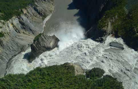
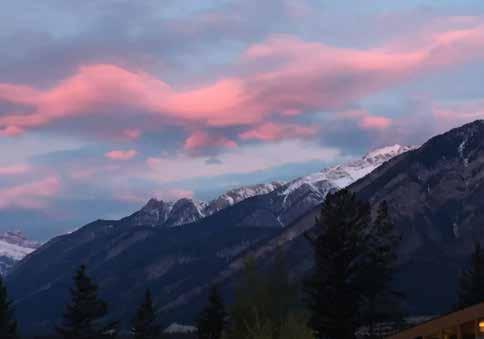
The conference dinner that evening was a great chance to network and discuss the ideas of the day. A more relaxed presentation on the Calgary Flood of 2013 (Noad) was preceded by thanks to the organizing committee and CSPG staff, as well as to the session chairs and speakers. It had been a great day, enhanced by the amazing weather, chilly yet with plenty of sunshine (see the photo from sunrise the following morning).
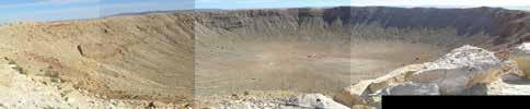
The final day of the conference began with the deep-water session. A fascinating presentation on a Nova Scotian impact crater (Deptuck) got everyone engrossed, followed by a talk on flow criticality in turbidites and its contrast in process style to open channel flow (Arnott) Bill impressed everyone by carrying on speaking through two power cuts that plunged the auditorium into complete darkness. The following talk on flow monitoring in BC fjords (Clarke) was similarly affected, but did not stop us seeing some great images of crescentshaped dunes and channel migration year on year. The last three talks all looked at submarine channels, contrasting the meandering morphology of submarine channels with those in the fluvial realm. The modeling of these systems (Sylvester) is complex, and was complemented by outcrop studies focused on the Gulf Islands of BC (Hubbard) and Chile (Southern).
After lunch we waded into the mud,
beginning with a nice overview of Devonian mudstones (Harris). Talks on aggregate grains and their use in differentiating marine and terrestrial deposits (Cheadle, Pavan) were followed by an interesting discussion of condensed sections (AlMufti). A general overview on data analysis in unconventional shale deposits centred on the Woodford Shale (Slatt) set the stage for a presentation that showed how sequence stratigraphy could be related to brittle/ductile contrasts in the unit (Jing). The mud session concluded the conference
We must definitely mention the outstanding posters presented on diverse topics ranging from Cretaceous meander belts (Durkin, Broughton) to estuarine facies models of the McMurray (Fustic); deposition and diagenesis of mudstones (Percy) and sequence stratigraphy of Horn River mudstones (Ayranci); to dating of shelf margin evolution using zircons (Daniels) and deep-marine channel evolution (Arnott).
Overall this was a stunning conference. The number of participants (around 66) ensured a fairly intimate atmosphere that helped to generate discussion, while the presence of many world-class sedimentologists ensured that the data presented, and the talks themselves, were of the highest quality. The geological discussions over a few beers in the evenings were worth the entrance price on their own. If you were not able to attend, you missed a conference that will be talked about for many years to come.
30 RESERVOIR ISSUE 11 • DECEMBER 2016 SOCIETY ARTICLE


RESERVOIR ISSUE 11 • DECEMBER 2016 31 Did you know there is over $20,000 available in CSPG awards and scholarships?! STUDENTS! Please visit www.cspg.org/students for more information Scholarship/Award Amount Available Application Deadline Regional Graduate Student Scholarships ($2,500 x 4) January 20, 2017 Undergraduate Student Awards ($1,000 x 4) January 20, 2017 Student Event Grants ($1,000 x 5) March 17, 2017 Andrew Baillie Award ($1,000 x 2) GeoConvention 2017

The 2017 Mountjoy Conference sponsored by SEPM (Society for Sedimentary Geology) and CSPG (Canadian Society of Petroleum Geologists) will be held the week of June 26-30, 2017 in Austin, Texas, at the University of Texas Commons Learning Center and the Bureau of Economic Geology Core facility.
The Technical Program Committee (David Budd, Gregor Eberli, Cathy Hollis, Don McNeill, Gene Rankey, Rachel Wood) on behalf of the SEPM and CSPG, is very pleased to announce that the ABSTRACT SUBMISSION IS NOW OPEN for the 2nd Mountjoy Carbonate Research Conference!
The theme of the meeting is "Carbonate Pore Systems”.
The meeting will be a mix of oral and poster presentations (Monday and Thursday), an in-meeting fieldtrip (Tuesday), and a full-day core workshop (Wednesday). The meeting will provide abundant time for discussion and interaction with the technical presenters and attendees. Those attending the Conference will gain an improved understanding of porosity at variable scales in carbonate rocks. Registration for the meeting opens in February, 2017 and is capped at 150 people maximum. Details of the meeting, and the trips, are located at http://www.sepm.org/MountjoyII
In a glance, the technical sessions and session Chairs include:
Sedimentological, Stratigraphic, and Diagenetic Controls on Development of Carbonate Pore Systems
Mike Grammer | Oklahoma State University James Bishop | Chevron David Budd | University of Colorado
Microporosity
in
Conventional and Unconventional Carbonate Reservoirs
Steve Kaczmerak | Western Michigan University Gregor Baechle | Consultant, Houston, TX Bob Loucks | BEG University of Texas
Multiscale Prediction and Upscaling of Carbonate Porosity and Permeability
Neil Hurley | Chevron Ralf Weger | University of Miami Beth Vandenberg | British Petroleum (BP)
Interactions in Multi-Modal Pore Systems
Bob Goldstein | University of Kansas Charlie Kerans | BEG University of Texas Alex MacNeil | Osum Oil Sands Co.
Visualization, Quantification, and Modeling of Carbonate Pore Systems and Their Fluid Flow Behavior
Paul M. (Mitch) Harris | University of Miami / Rice University Gregor Eberli | University of Miami Gareth Jones | ExxonMobil
The technical committee would also like to invite submission of abstracts for the all-day core. Cores representing a spectrum of geologic time and depositional settings, as well as unique diagenetic environments from some of the most significant producing reservoirs will be on display. The cores will be highlighted in a core preview display during the technical sessions on Monday. Wednesday will be the full core display and discussion with presenters at the Austin Core Research Center (CRC), located adjacent to the University of Texas, Bureau of Economic Geology headquarters.
The core workshop represents a great way to see examples of all sorts of different reservoirs, and to get your hands on the rock. The core displays will demonstrate important aspects of reservoir quality of both conventional and unconventional carbonate reservoirs.
For any questions, feel free to contact the conference General Chair or any of the Technical Program chairs:
General Chair: Paul (Mitch) Harris | pmitchharris@gmail.com
Technical Program Chairs: Don McNeill | dmcneill@rsmas.miami.edu Gene Rankey | grankey@ku.edu
Core Conf. Chair: Laura Zahm | laz@statoil.com
Field Trip Chair: Astrid Arts | astrid.arts@cenovus.com