$10.00 DECEMBER 2015 VOLUME 42, ISSUE 11 Canadian Publication Mail Contract – 40070050 RETURN UNDELIVERABLE CANADIAN ADDRESSES TO: CSPG – 110, 333 - 5 Avenue SW Calgary, Alberta T2P 3B6 Addressee Additional Delivery Information Street Address Postal Box Number and Station Information Municipality, Province/Territory Postal Code 14 Geomodeling: A Team Effort To Better Understand Our Reservoirs Part 6: Geophysicists And Geomodeling 21 Annual Young Geoscientists Networking Reception 22 Gussow Conference 2015 Fine Grained Clastics: Resources to Reserves Meeting Summary
Geomodeling: A Team Effort To Better Understand Our Reservoirs
CSPG OFFICE
#110, 333 – 5th Avenue SW Calgary, Alberta, Canada T2P 3B6
Tel: 403-264-5610
Web: www.cspg.org
Please visit our website for all tickets sales and event/course registrations Office hours: Monday to Friday, 8:00am to 4:30pm
The CSPG Office is Closed the 1st and 3rd Friday of every month.
OFFICE CONTACTS
Membership Inquiries
Tel: 403-264-5610 Email: membership@cspg.org
Technical/Educational Events: Biljana Popovic
Tel: 403-513-1225 Email: biljana.popovic@cspg.org
Advertising Inquiries: Kristy Casebeer
Tel: 403-513-1233 Email: kristy.casebeer@cspg.org
Sponsorship Opportunities: Lis Bjeld
Tel: 403-513-1235 Email: lis.bjeld@cspg.org
Conference Inquiries: Candace Jones
Tel: 403-513-1227 Email: candace.jones@cspg.org
CSPG Foundation: Kasandra Amaro
Tel: 403-513-1234 Email: kasandra.amaro@cspg.org
Accounting Inquiries: Eric Tang
Tel: 403-513-1232 Email: eric.tang@cspg.org
Executive Director: Lis Bjeld
Tel: 403-513-1235, Email: lis.bjeld@cspg.org
EDITORS/AUTHORS
Please submit RESERVOIR articles to the CSPG office. Submission deadline is the 23rd day of the month, two months prior to issue date. (e.g., January 23 for the March issue).
To publish an article, the CSPG requires digital copies of the document. Text should be in Microsoft Word format and illustrations should be in TIFF format at 300 dpi., at final size.
CSPG COORDINATING EDITOR
Kristy Casebeer, Programs Coordinator, Canadian Society of Petroleum Geologists
Tel: 403-513-1233, kristy.casebeer@cspg.org
The RESERVOIR is published 11 times per year by the Canadian Society of Petroleum Geologists. This includes a combined issue for the months of July and August. The purpose of the RESERVOIR is to publicize the Society’s many activities and to promote the geosciences. We look for both technical and non-technical material to publish. The contents of this publication may not be reproduced either in part or in full without the consent of the publisher. Additional copies of the RESERVOIR are available at the CSPG office.
No official endorsement or sponsorship by the CSPG is implied for any advertisement, insert, or article that appears in the Reservoir unless otherwise noted. All submitted materials are reviewed by the editor. We reserve the right to edit all submissions, including letters to the Editor. Submissions must include your name, address, and membership number (if applicable).The material contained in this publication is intended for informational use only.
While reasonable care has been taken, authors and the CSPG make no guarantees that any of the equations, schematics, or devices discussed will perform as expected or that they will give the desired results. Some information contained herein may be inaccurate or may vary from standard measurements. The CSPG expressly disclaims any and all liability for the acts, omissions, or conduct of any third-party user of information contained in this publication. Under no circumstances shall the CSPG and its officers, directors, employees, and agents be liable for any injury, loss, damage, or expense arising in any manner whatsoever from the acts, omissions, or conduct of any third-party user.
Printed by McAra Printing, Calgary,
Alberta.
Gussow Conference 2015
FRONT COVER
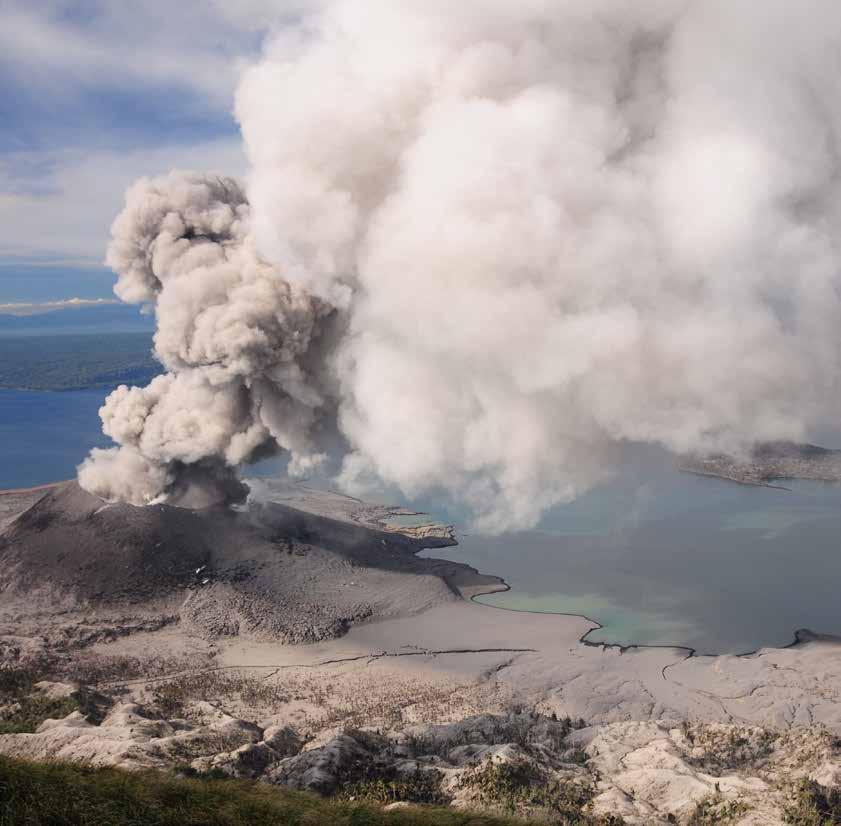
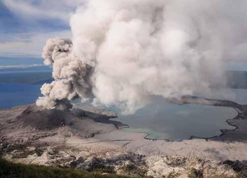
Tavurvur is a stratovolcano within the Rabaul caldera, located at the eastern tip of New Britain Island, Papua New Guinea.
Explosive eruptions have occurred persistently since 1994, repeatedly covering the town of Rabaul and surrounding area in fine, powdery ash.
Photo by: Nicholson, Paul G. DECEMBER 2015 – VOLUME 42, ISSUE 11 ARTICLES
Part
Geophysicists And
14 Annual Young Geoscientists Networking Reception 21
6:
Geomodeling
Fine
Resources to Reserves Meeting Summary ............................... 22 Honorary Member - Graeme Bloy 26 DEPARTMENTS Message from the Board 5 Technical Luncheons ................................................................................................................... 8 Division Talks .............................................................................................................................. 11 Rock Shop 25 RESERVOIR ISSUE 11 • DECEMBER 2015 3
Grained Clastics:


Speaker: Steve Grasby | Geological Survey of Canada
Tuesday December 8th , 2015
Wine & Appetizers 10:30-11:30am Technical Luncheon 11:30-1:00pm
This is a sellout social event that you don’t want to miss!
Tickets are available at www.cspg.org

Sponsored by:

CSPGandgeoLOGICSystemsPresentour Annual Holiday Social & Technical Luncheon Talk: Glacier Gas– ImpactofContinental GlaciationonSedimentaryBasins
CSPG BOARD


PRESIDENT
Tony Cadrin president@cspg.org Tel: 403.303.3493
PRESIDENT ELECT
Greg Lynch • Shell Canada Ltd presidentelect@cspg.org Tel: 403.384.7704
PAST PRESIDENT
Dale Leckie pastpresident@cspg.org
FINANCE DIRECTOR
Astrid Arts • Cenovus Energy directorfinance@cspg.org Tel: 403.766.5862
FINANCE DIRECTOR ELECT
Scott Leroux • Long Run Exploration directorfinanceelect@cspg.org Tel: 403.802.3775
DIRECTOR
Mark Caplan conferences@cspg.org
DIRECTOR
Milovan Fustic • Statoil Canada Ltd. publications@cspg.org Tel: 403.724.3307
DIRECTOR
Michael LaBerge • Channel Energy Inc. memberservices@cspg.org Tel: 403.301.3739
DIRECTOR
Ryan Lemiski • Nexen Energy ULC ypg@cspg.org Tel: 403.699.4413
DIRECTOR
Robert Mummery • Almandine Resources Inc. affiliates@cspg.org Tel: 403.651.4917
DIRECTOR
Darren Roblin • Kelt Exploration corprelations@cspg.org Tel: 587.233.0784
DIRECTOR
Jen Russel-Houston • Osum Oil Sands Corp. Jrussel-houston@osumcorp.com Tel: 403.270.4768
DIRECTOR
Eric Street • Jupiter Resources street@jupiterresources.com Tel: 587.747.2631
EXECUTIVE DIRECTOR
Lis Bjeld • CSPG lis.bjeld@cspg.org Tel: 403.513.1235
Message from the Board
A message from Astrid Arts, Finance Director
Financial Overview of the CSPG 2015 Fiscal Year
The CSPG 2015 fiscal year ran from September 1, 2014 through to August 31, 2015.
A lot can happen in a year.WTI went from US $92.92 to US $49.20, the Canadian dollar went from $0.91 to $0.76 US and over 35,000 people in Alberta lost their jobs in the petroleum industry. Albertans elected an NDP government in May who increased corporate and personal income taxes and have left an air of uncertainty over our industry. The CSPG is registered federally under the NotFor-Profit Act and so as an organization we won’t feel an added tax burden but we recognize that many of our members, corporate sponsors, advertisers and exhibitors will. We are in a recession unlike any we have seen since the 1980’s. Most companies are not projecting WTI prices to turn around until 2017 but even that may be bullish. How long this will last is anybody’s guess.
The CSPG has felt the effects of the downturn. On the whole though, we are in good financial shape to weather the storm thanks to the solid work of many past CSPG Finance Directors, CSPG Executives as well as Lis, Eric and the rest of the CSPG office staff. Savings during profitable years has positioned the CSPG with an Internally Restricted Rainy Day fund of $1.1 MM and an unrestricted fund of $720 K at year end. Our portfolio is conservatively invested where we hold an asset mix of 80% Fixed Income and 20% Equities on an Adjusted Cost Base. Operationally, we brought in $1.9 MM in Revenue and had $2.2 MM in Expenses. Fully audited Financial Statements will be available on the cspg.
org website by the end of December if you are curious about all the details. For 2015 we posted a loss of ~$230 K, quite a swing from the ~$175 K profit we made in fiscal year 2014. Most of that loss was the result of reduced sponsorship, lower attendance at our events, donation to CSPG Foundation and a reduced profit from the GeoConvention Partnership. Nothing unexpected in a downturn.
As a Not-For-Profit society our metrics for success are different than the E&P and Service companies many of our members work for. The mission of the CSPG is to advance the professions of the energy geosciences – as it applies to geology, foster the scientific, technical learning and professional development of its members; and promote the awareness of the profession to industry and the public. As a society we accomplish this through the tireless work of volunteers in 40+ committees, it is astounding what our CSPG community accomplishes and it is something we should all be proud of. Some highlights of our activities from 2015:
• 16 Technical Luncheons, Fall & Spring Education Weeks & a Gussow Conference on Geomodelling
• The GeoConvention Partnership ran its first geoConvention since its formation as its own legal entity in which CSPG has a 45% ownership (along with CSEG 45% and CWLS 10%)
• Three Joint Venture Conferences
• Oil Sands with AAPG, Playmakers with AAPG & the inaugural Mountjoy Carbonate Conference with SEPM
(... Continued on page 7)
RESERVOIR ISSUE 11 • DECEMBER 2015 5
Submit your hike to be featured in the
“GO TAKE A HIKE” SERIES
Before writing an article please contact the series coordinator via email at Philip.Benham@shell.com. He can provide a template document and confirm that a particular hike has not been submitted before.
Submission guidelines:
Preferred format is powerpoint, 2-3 pages in length, include map, hike directions, annotated photos, Geological description and references. While hikes focus on western Canada, hikes in other parts of the world are welcome.

CSPG Regional Graduate Student Scholarships
4 x $2,500 awards available by region (Atlantic/Quebec, Ontario, Western, Open)
Eligibility:
Graduate Students enrolled full-time at a Canadian University in their first year of an MSc or PhD Geology or Earth Science Program
Disciplines include: Sedimentology, structural geology, stratigraphic studies involving clastic or carbonate rocks, paleontology, geochemistry, hydrogeology, petrophysics and reservoir geology
Active student members of CSPG (membership is free!)
Previous winners are not eligible
Application deadline is January 15, 2016
For application form and other requirements please see www.cspg.org/scholarships
CORPORATE SPONSORS
SAMARIUM
CSPG Foundation
geoLOGIC systems ltd.
DIAMOND
AGAT Laboratories
Alberta Energy Regulators
TITANIUM
Tourmaline Oil Corp.
APEGA
PLATINUM
Weatherford Canada Partnership
Cenovus Energy
Loring Tarcore Labs Ltd.
Imperial Oil Resources
SILVER
Devon Energy Corp
Enerplus Corporation
Nexen ULC
Seitel Canada Ltd.
MEG Energy Corp.
Husky Energy Inc.
BRONZE
Chinook Consulting
Talisman Energy
Long Run Exploration
Qatar Shell GTL Limited
Osum Oil Sands Corp.
Crescent Point Energy Trust
Pro Geo Consultants
Exxonmobil Exploration Co. Ltd.
Belloy Petroleum Consulting
GLJ Petroleum Consultants Ltd.
Gaffney, Cline & Associates
RIGSAT Communications
CSEG Foundation
MJ Systems
Paradigm Geosciences Ltd.
Core Laboratories
IHS Global Canada Limited
(... Continued from page 5)
• 4 sporting events
• Road Race & Fun Run, Squash Tournament, Mixed Golf and Classic Golf Tournaments (Classic moved to a new 1 day format)
• Continued investment in our Young Professional and Outreach programs and we launched the CSPG Ambassador program which is working on improving our relationships with universities and organizations across the country.
• $75 K donation to the CSPG Foundation (from 2014 Audited Profits)
Looking forward into the 2016 Fiscal Year we are looking at ways to adjust
our programs to best meet our member needs in this new environment. We recognize that our community is one of our biggest strengths and our society and industry will be forever different when prices rebound. Our demographics will have changed as many of our members retire. New grads, young and seasoned professionals who have struggled to find work over the last year, may choose to leave industry and the profession. As a society we have money in the bank to pay for our activities for a few more years at current spending levels but we have challenged our committees to see what they can do this year with 80% of their budgets. This is the 88th year of our society and if there is one thing we can say with certainty, it is that every time the price of oil goes down … it always goes back up.

RESERVOIR ISSUE 11 • DECEMBER 2015 7
As
Ocotber 30, 2015
Geologic
Ltd., CSPG’s Top
the
of
A Special Thanks to
Systems
Sponsor of
Month.
TECHNICAL LUNCHEONS DECEMBER LUNCHEON
Glacier Gas - Impact of continental glaciation on sedimentary basins
SPEAKER
Steve Grasby Geological Survey of Canada
11:30 am
Tuesday, December 8th, 2015 Calgary, TELUS Convention Centre Macleod Hall ABC Calgary, Alberta
Please note: The cut-off date for ticket sales is 1:00 pm, five business days before event. [Tuesday, December 01, 2015].
CSPG Member Ticket Price: $45.00 + GST. Non-Member Ticket Price: $47.50 + GST.
Each CSPG Technical Luncheon is 1 APEGA PDH credit. Tickets may be purchased online at www.cspg.org
ABSTRACT
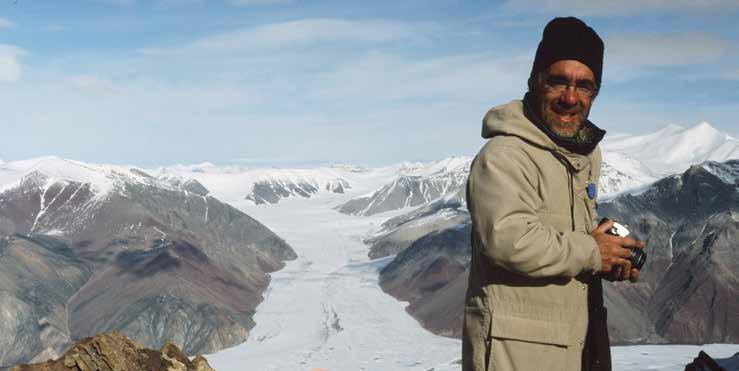
Northern hemisphere continents were covered by ice sheets up to 4 km thick during the last glacial period. Until recently the impact this had on sedimentary basins has been largely ignored. The underlying bedrock was exposed to both the lithostatic load of ice in addition to tremendous sub-glacial water pressures. This has a significant transitory effect on underlying sedimentary basins. Where overlying more porous and permeable units, subglacial waters were injected into underlying sediments, reversing continental-scale fluid flow systems. Therefore relic pressure distribution patterns in the modern basins reflect gradual recovery of the basin hydrodynamics flow system in response to offloading of ice, and are not related to longer term fluid migration that drove oil and gas migration. Injection of fresh waters also flushed saline fluids from the rock systems, creating conditions more suitable for methanogenesis and in some cases has initiated biogenic formation of economic methane accumulations. Fresh waters injection has also lead to subsurface dissolution of evaporite beds and the formation of salt collapse features. Post glaciation establishment of new flow systems has led to gradual flushing of these glacial waters from sedimentary basins, in some areas they still represent a significant source of potable water that may not be readily be replenished by modern recharge. At the other extreme, glacial waters that have dissolved
salt beds now discharge as saline springs along the basin margins. Highly overpressured conditions, developed in response to subglacial water pressures, also provide opportunities to examine the response of shales to extreme cases of fluid injection that may inform discussion on issues ranging from shale gas development to nuclear waste repositories.
BIOGRAPHY
Steve Grasby - Since completion of his Ph.D at the University of Calgary in 1997, Dr. Grasby has worked at the Geological Survey of
Canada on both source rock analyses as well as groundwater issues across western and northern Canada. He has led and participated on several regional groundwater projects, including southern Manitoba, Alberta, the Okanagan Valley, and currently the Nanaimo Lowlands. In addition he has conducted extensive research on the biogeochemistry of thermal and mineral springs across Canada, including several of the northern most known springs in Canada’s High Arctic. He was awarded the Queen Elizabeth II Diamond Jubilee Medal in recognition of his research in 2012.
CRAINʼS LOG ANALYSIS COURSES For Engineers, Geologists, Geophysicists, and Technologists Every April and Octoberin Calgary Details /Registration at www.spec2000.net/00-coursedates.htmSlide Shows, Reference Manuals, and Exercises Included AV-01 Practical Quantitative Log Analysis AV-02 Advanced Quantitative Log Analysis AV-03 Analysis of Unconventional Reservoirs Details / Order Onlineat: www.spec2000.net/00-av-training.htm Single-User, Corporate, and Academic Licenses Available Individual Reference Manuals and Slide Shows Available Separately Shareware Petrophysical Encyclopediaat www.spec2000.net 50+ Years OfExperience AtYour Fingertips === E. R. (Ross) Crain. P.Eng. 1-403-845-2527 ross@spec2000.net === === 8 RESERVOIR ISSUE 11 • DECEMBER 2015
Webcasts sponsored by
TECHNICAL LUNCHEONS JANUARY LUNCHEON
Back for more?
The first Permian oil discovery in the Barents Sea has many analogues in the Sverdrup Basin, Arctic Canada
SPEAKER
Benoit Beauchamp Department of Geoscience, University of Calgary, Calgary, Alberta 11:30 am
Thursday, January 14, 2016 Calgary, TELUS Convention Centre Calgary, Alberta
Please note: The cut-off date for ticket sales is 1:00 pm, five business days before event [Thursday, January 07, 2016]. CSPG Member Ticket Price: $45.00 + GST. Non-Member Ticket Price: $47.50 + GST.
Each CSPG Technical Luncheon is 1 APEGA PDH credit. Tickets may be purchased online at https://www.cspg.org
ABSTRACT
The 2013 Gohta oil discovery is the first significant discovery in the Permian succession
of the Barents Sea. The oil pool lies beneath a sub-Early Triassic angular unconformity, suggesting block faulting and tilting prior to the onset of Triassic sedimentation. The reservoir rocks are Permian spiculitic cherts and heterozoan carbonates of shallow origin that accumulated at a time of cool oceanographic conditions. The porosity may be the result of extensive sub-Triassic subaerial karsting. The seemingly unique set of attributes of the the Gohta Discovery has been observed at a number of localities in the Canadian Arctic Archipelago. The Sverdrup Basin was adjacent to the Barents Sea area throughout its Late Paleozoic-Mesozoic history prior to the break-up of Pangea. The succession is thicker than that of the Barents Sea, owing to greater subsidence rates, but its stratigraphic sequences are identical. Permian spiculitic chert is widespread, especially in the Late Permian succession, when carbonates were all but eradicated.The loss of carbonates can be in part associated with cooler oceanic conditions and possibly to upwelling-enhanced ocean acidification along NW Pangea. Late Permian organic-rich shales locally interfinger with the chert and may constitute a source rock. Porosity is unusually high in Late Permian chert. Large carbon isotopic depletion in carbonate material beneath the sub-Triassic unconformity suggests extensive meteoric leaching occurred. The sub-Triassic unconformity is widespread and one of the basin’s most significant in terms of base level drops.The unconformity is also locally angular and associated with basal conglomerates of
Permian pebble to cobble spiculitic chert clasts. An angular relationship is observed on northern Ellesmere and Axel Heiberg islands. From these observations we conclude the set of conditions that led to Gohta is a genuine play worth exploring some more in the Barents Sea and, when conditions are right, in the Sverdrup Basin as well.
BIOGRAPHY
Benoit is a Professor of Geoscience at the University of Calgary. He obtained his undergraduate and M.Sc. degrees in geology at the Université de Montréal studying Carboniferous carbonates from Western Canada. Subsequently, he moved to Calgary to pursue a Ph.D. in geology at the University of Calgary. For his dissertation, he studied Carboniferous and Permian sedimentary rocks in the Canadian Arctic. After obtaining his Ph.D. in 1987, Benoit worked for 18 years as a Research Scientist with the Geological Survey of Canada in Calgary, leading major field expeditions to the High Arctic. In 2005, he became the Executive Director of the Arctic Institute of North America at UofC. In 2011, he returned to the Department of Geoscience as a full-time professor. Much of Benoit’s research interests revolve around understanding the Late Paleozoic-Early Triassic sequences and petroleum systems, which takes him to exotic places such as Ellesmere Island, Svalbard and Oman. Benoit has been an active contributor to many CSPG events and endeavours over the years, including his leadership roles in the 1993 and 1997 CSPG Conventions and in the 2007 Gussow Conference.
RESERVOIR ISSUE 11 • DECEMBER 2015 9
Webcasts sponsored by
TECHNICAL LUNCHEONS JANUARY
Antarctica’s sedimentary archives of past glacial history: Tools for understanding climate change
SPEAKER
Julia Wellner
AAPG Distinguished Lecturer
11:30 am
Tuesday, January 26, 2016 Calgary, TELUS Convention Centre Calgary, Alberta
Please note: The cut-off date for ticket sales is 1:00 pm, five business days before event [Tuesday, January 19, 2016].
CSPG Member Ticket Price: $45.00 + GST. Non-Member Ticket Price: $47.50 + GST.
Each CSPG Technical Luncheon is 1 APEGA PDH credit. Tickets may be purchased online at https://www.cspg.org
ABSTRACT
During times of past extensive glaciations, the Antarctic ice sheet extended from its current position, reaching across the continental shelf. As the ice sheet retreated to its modern extent, the shrinking ice sheet left behind seawater, rather than ancient ice, leaving behind a sedimentary signature of deglacial history. Marine geophysical survey data, including 3.5 kHz profiles and multibeam swath bathymetry, combined with sediment cores, are used to map the extent of past ice, estimate the speed at which it was flowing, and understand the style of retreat. Radiometric dating gives ages of retreat and allows comparison to other global archives. Past periods of glacial retreat, which tend to be diachronous, are compared to the modern day retreat, which is happening across large areas in a short period of time. Ongoing work is targeting records from times of past high
CO2 conditions, like those predicted in our future.
BIOGRAPHY
Julia Wellner - Wellner is a sedimentologist and stratigrapher who works primarily in the Gulf of Mexico and offshore Antarctica on questions related to sediment facies, stratigraphic architecture, glacial history, and sea-level change. She earned her PhD from Rice University in 2001 where she also completed a post-doctoral fellowship. She has been at the University of Houston since 2006 where she teaches stratigraphy, sequence stratigraphy, marine geology, and oceanography. Wellner has completed over a dozen ocean-going cruises collecting seismic data and sediment cores, including eight in Antarctica.
GeoConvention 2016

With low commodity prices and an everchanging economic and business environment, it is imperative that the industry optimize the way in which it operates. Whether enhancing recovery methods, finding the optimal path for a horizontal well or maximizing the return of capital employed, Optimizing Resources, the theme for GeoConvention 2016, is key to success.
Please join us and contribute as speaker, exhibitor or sponsor In recognizing the business environment which we are operating in, GeoConvention is pleased to offer heavily discounted delegate rates for the 2016 program.


for our 2016 program, in addition to the technical program and exhibit floor at the Convention Centre, we will be hosting an offsite component at the Lake Louise Inn – check out geoconvention.com for details.
www.geoconvention.com
EARLY BIRD REGISTRATION NOW OPEN MARK YOUR CALENDAR GeoConvention 2016 is March 7 – 11 10 RESERVOIR ISSUE 11 • DECEMBER 2015
New
LUNCHEON Webcasts sponsored by
Husband and Wife survive an 18-Month Trip around Africa in a Land Cruiser
SPEAKER
Tom Feuchtwanger
12:00 Noon
Wednesday December 9th 2015
Buzzards Restaurant & Bar 140-10 ave SW, Calgary, AB T2R 0A3
ABSTRACT
In an attempt to seek adventure, escape the daily grind, and recharge their 30year marriage, exploration geologist Tom Feuchtwanger and healthcare professional Janet Wilson purchased a Land Cruiser in South Africa, modified it for extended selfsupported travel, and spent 18 months circumnavigating the African continent. He will present this once-in-a-lifetime adventure: its highs, its lows, and what they learned about
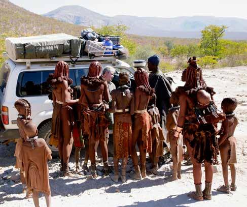
themselves and the world along the way. Tom will also include some comments about the
hydrocarbon resource opportunities and challenges that Africa is facing currently.
CSPG Structural Geology Division Lunchtime Talk
12:00-1:00pm | Thursday December 3, 2015
Schlumberger, Conference Room, Second Floor, Close to Reception, 200 125-9 Ave SE
Random Rocks, Structures and Geo IQ – Christmas Social
Just us in December for something different. Three things geologists love – rocks, structures and showing how brilliant they are!
We will be having a Christmas Quiz, with great photographs, brain teasers and cryptic clues. Put together a team of 2-3 people, give yourselves a good name, then come along and test your Geology IQ. See your friends, enjoy some snacks, have a bit of fun. Contest starts at 12 noon – sharp! All are welcome and no registration is required. Bragging rights for the winner! For more information go to www.cspg.org
RESERVOIR ISSUE 11 • DECEMBER 2015 11 DIVISION TALKS INTERNATIONAL DIVISION Sponsored by
Tom Feuchtwanger P.Geol.
DIVISION TALKS GEOMODELING DIVISION
Modeling three ways from electrofacies: categorical, e-facies probabilities, and petrophysics with assignment
SPEAKER
David Garner
Halliburton/Landmark
CO-AUTHORS
R. Mohan Srivastava
FSS Canada Consultants
Jeffrey Yarus
Halliburton/Landmark
12:00 noon
Wednesday, December 9, 2015
Husky Conference Room A, 3rd Floor, +30 level, South Tower, v707 8th Ave SW, Calgary, Alberta
ABSTRACT
[This paper was previously presented at EAGE Petroleum Geostatistics Biarritz, France, 7-11 September 2015]
Geomodeling for petroleum reservoirs is conventionally done hierarchically by facies to establish regions within which rock and fluid properties can be considered “stationary”. Many reservoir models do not use depositional facies description, but use “electro-facies” from clustering of petrophysical log curves. This paper compares three approaches to the development of e-facies geomodels, 3D models of categorical codes that can be used as stationary domains within which rock and fluid properties can be simulated. The first approach takes the e-facies codes developed through cluster analysis as conditioning data and uses a method for simulating categorical variables, plurigaussian simulation, to directly build a 3D model of the e-facies. The second approach takes the petrophysical logs at the wells as conditioning data and uses a standard method for co-simulating continuous variables, to build 3D models of the log responses; these are then converted to e-facies using the rules developed through cluster analysis. The third method works directly with the e-facies probabilities that most cluster analysis techniques can provide. These probabilities are co-simulated as
DIVISION TALKS BASS DIVISION
Data
Integration Techniques for Geocellular Model Building, An Example from the McMurray
SPEAKER
Pippa Murphy
Schlumberger Canada
12:00 noon
Tuesday December 15, 2015 | 12:00pm
ConocoPhillips Auditorium, Gulf Canada Square, 401-9th ave SW Calgary AB
ABSTRACT
In order to accurately simulate the movement of a steam chamber through the McMurray
formation, we need to be able to capture the complex heterogeneity of the geology within these models. We also need to gather a firm understanding of the distribution of gas and water that may have an effect on the ability of these steam chambers to grow.
The aim of the game is always to honor the information at the wells whilst achieving sound results in terms of geostatistics. But what other information could we use to increase our confidence in the models that we are building, and could we use some of this data to impose a more geological flavor to our models rather than relying on the fully stochastic population techniques that we commonly see today.
During this talk we’ll look at an example model where geological analogues, as well as data derived from seismic have come together to build a realistic and confident model of the McMurray which can then be used for simulation and field development going forward.
continuous variables in 3D, ensuring they are bounded and sum to 1, and a unique e-facies code is assigned, by taking the e-facies with the maximum probability at each location.
BIOGRAPHY
David Garner is a chief scientist and technical advisor with the Landmark R&D Division of Halliburton. His current focus is mainly on developing new technologies and filling gaps in integrated subsurface earth modeling. David has previously worked in R&D at Statoil and in various geomodeling/geostatistical roles at Chevron, ConocoPhillips and his old consulting company, TerraMod Consulting.
Mr. Garner currently serves as a co-chair for the Geomodeling Technical Division of the CSPG. He previously served on the CSPG board of directors and was general chair for the Gussow 2011 and 2014 conferences, “Advances in Applied Geomodeling for Hydrocarbon Reservoirs: Closing the Gap I and II”.
INFORMATION
There is no charge for the division talk and we welcome non-members of the CSPG. Please bring your lunch. For details or to present a talk in the future, please contact Weishan Ren at renws2009@gmail.com
BIOGRAPHY
Pippa Murphy is a Geoscience Consultant and Petrel expert with Schlumberger Canada. She started her career with Schlumberger in 2005 as a technical consultant working on multiple international plays out of the UK. Now based in Calgary, Pippa works closely with oil and gas companies to leverage the full range of capabilities in Schlumberger software to solve their exploration and development challenges. She is currently engaged in a number of heavy oil related projects. Pippa is a Geologist by background and studied at Kingston University in London, England.
INFORMATION
BASS Division talks are free. Please bring your own lunch. For further information about the division, joining our mailing list, a list of upcoming talks, or if you wish to present a talk or lead a field trip, please contact either Steve Donaldson at 403-808-8641, or Mark Caplan at 403-9757701, or visit our web page on the CSPG website at http://www.cspg.org.
12 RESERVOIR ISSUE 11 • DECEMBER 2015
Sponsored by
Sponsored by
DIVISION TALKS PALAEONTOLOGY DIVISION
Sue (the Tyrannosaurus Rex) and the Chicago Field Museum
SPE A KER
Mona Marsovsky
APS Executive Member and Professional Engineer
7:30pm
Friday, January 15, 2016 Mount Royal University, Room B108
ABSTRACT
In the 1990’s controversy erupted around the Tyrannosaurus Rex (T-Rex) dinosaur named Sue. This included seizure of Sue’s skeleton by the FBI (Federal Bureau of Investigation), court hearings which resulted in a jail sentence for the person who excavated Sue’s skeleton, and an
auction in which Sue sold for more than 8 million dollars to the Field Museum in Chicago with the bill footed by the Ronald McDonald House and Disney. After years of preparation by staff and volunteers at the Field Museum in Chicago, Sue is now proudly displayed at the Field Museum. Mona will present an overview of Sue’s background and some of the things that Sue has taught us (scientific and otherwise). Mona will also illustrate some of the other treasures in the Chicago Field Museum.
BIOGRAPHY
Mona Marsovsky is a life member of the APS who has served as the APS treasurer since 2002. She is also a member of the Society of Vertebrate Paleontology. She is an amateur whose paleo habit has been supported by her work as a professional engineer (Mona Trick P. Eng.) programming gas and oil field optimization software for the oil industry. As part of her work, she has taught training courses and given luncheon talks all over the world.
GEOEDGES INC.
Detailed and accurate geology at your fingertips in Petra, GeoGraphix, ArcGIS, AccuMap, GeoScout and other applications
US Rockies & Williston Basin Geological Edge Set
US / Appalachian Basin Geological Edge Set
American Shales Geological Edge Set (all colors)
Mexico Geological Edge Set
Texas & Midcontinent US Geological Edge Set
INFORMATION
This event is presented jointly by the Alberta Palaeontological Society, the Department of Earth and Environmental Sciences at Mount Royal University, and the Palaeontology Division of the Canadian Society of Petroleum Geologists. For details or to present a talk in the future, please contact CSPG Palaeontology Division Chair Jon Noad at jonnoad@hotmail. com or APS Coordinator Harold Whittaker at 403-286-0349 or contact programs1@ albertapaleo.org. Visit the APS website for confirmation of event times and upcoming speakers: http://www.albertapaleo.org/.
information contact: Joel Harding at 403 870 8122 email joelharding@geoedges.com www.geoedges.com
Western Canada: Slave Point, Swan Hills, Leduc, Grosmont, Jean Marie, Horn River Shales, Elkton, Shunda, Pekisko, Banff, Mississippian subcrops and anhydrite barriers in SE Sask., Bakken, Three Forks, Montney, Halfway, Charlie Lake, Rock Creek, Shaunavon, BQ/Gething, Bluesky, Glauconitic, Lloyd, Sparky, Colony, Viking, Cardium, CBM, Oilsands Areas, Outcrops
US Rockies & Williston: Red River, Mississippian subcrops & anhydrite barriers (Bluell, Sherwood, Rival, etc), Bakken, Three Forks, Cutbank, Sunburst, Tyler, Heath, Muddy, Dakota, Sussex, Shannon, Parkman, Almond, Lewis, Frontier, Niobrara, Mesaverde shorelines, Minnelusa, Gothic, Hovenweep, Ismay, Desert Creek, Field Outlines, Outcrops
Texas & Midcontinent: Granite Wash, Permian Basin paleogeography (Wolfcampian, Leonardian, Guadalupian), Mississippian Horizontal Play, Red Fork, Morrow, Cleveland, Sligo/Edwards Reefs, Salt Basins, Frio, Wilcox, Eagleford, Tuscaloosa, Haynesville, Fayeteville-Caney, Woodford, Field Outlines, Outcrops, Structures
North American Shales: Shale plays characterized by O&G fields, formation limit, outcrop, subcrop, structure, isopach, maturity, stratigraphic crosssections. Includes: Marcellus, Rhinestreet, Huron, New Albany, Antrim, UticaCollingwood, Barnett, Eagleford, Niobrara, Gothic, Hovenweep, Mowry, Bakken, Three Forks, Monterey, Montney, Horn River, Colorado
Eastern US / Appalachia: PreCambrian, Trenton, Utica-Collingwood, MedinaClinton, Tuscarora, Marcellus, Onondaga Structure, Geneseo, Huron, Antrim, New Albny, Rhinestreet, Sonyea, Cleveland, Venango, Bradford, Elk, Berea, Weir, Big Injun, Formation limits, Outcrops, Allegheny Thrust, Cincinatti Arch, Field outlines
Mexico: Eagle Ford-Agua Nueva, Pimienta, Oil-Gas-Condensate Windows, Cupido-Sligo and Edwards Reefs, Tuxpan Platform, El Abra-Tamabra facies, Salt structures, Basins, Uplifts, Structural features, Sierra Madre Front, Outcrops, Field Outlines
Deliverables include:
-Shapefiles and AccuMap map features
-hard copy maps, manual, pdf cross-sections
-Petra Thematic Map projects, GeoGraphix projects, ArcView map and layers files
-bi-annual updates and additions to mapping
-technical support
Western
Northern
Eastern
Canada Geological Edge Set
North
for
RESERVOIR ISSUE 11 • DECEMBER 2015 13
Sponsored by
GEOMODELING: A TEAM EFFORT TO BETTER UNDERSTAND OUR RESERVOIRS
Part 6: Geophysicists and Geomodeling
| By Thomas Jerome, RPS, Sher Ali, Brion Energy and Nilanjan Ganguly, Canacol Energy
INTRODUCTION
After discussing, in the last two papers, how geologists and petrophysicists can get involved in a geomodeling project, we now look at the role of geophysicists.This paper is the last one on the relationships between geoscientists and geomodelers. The next three papers will talk about the role of engineers.
Geophysicists in oil and gas companies worked mostly on 2D seismic data before the technology to acquire 3D seismic data was developed and became popular. Companies are now also using seismic data to monitor the development of their fields thanks to the acquisition of 4D seismic data. Nowadays, geomodelers still have to integrate some 2D seismic lines into their models and some are starting to work on the integration of 4D time-lapse data. But for most of us, when we think about geophysical data, we have in mind the integration of 3D seismic data into our geomodels. This topic is the focus of this paper.
First, one has to ask: Why do we need a geomodel if we have acquired 3D seismic data? After all, seismic cubes give us an image of our reservoirs between the wells. Don’t they solve all of our problems? Using a technology as a stand-alone product has its use. When integrated with other technologies, such as geomodeling, that is
when it shows its potential.
A seismic cube does give us a 3D image of the reservoir; however, the resolution is usual too low to capture the level of detail engineers need to truly understand the reservoir. Wells data provides the level of detail we are looking for, but this data can be cumbersome to interpolate in 3D. The solution is to integrate well data and seismic data.
We use trends extracted from seismic to guide the interpolation of wells data in 3D. Some uncertainty about the reservoir will remain, coming both from the seismic interpretation process, from the work on the wells and from the integration of the well data with the seismic. This uncertainty needs to be taken into account as well. Integrating different type of data together and understanding the impact of uncertainties in a model: these are two tasks that geomodels are designed for.
As such, it’s advisable to build a geomodel whenever seismic data and seismic interpretation are available. In the meantime, building a geomodel only based on well data while seismic is readily available would be a shame. Good seismic information will always tell us more about the reservoir than the results of pure mathematical interpolation techniques. If a geomodel is about to be built, a geomodeler should always ask if seismic data are available.
Geomodeling can be used for time-to-depth conversion. This will be covered in the first section. Secondly, seismic interpretation is extremely useful to guide how the geomodel 3D-grids shall be built. The second section focuses on the integration of stratigraphic interpretation, while the third section looks at the integration of structural interpretation in geomodeling. Lastly, considerable information about the rock characteristics can be extracted from the seismic cube, such as seismic attributes or fracture density for example. This data can be used to guide geostatistical algorithms. It will be the topic of the last section. Each of these sections will also cover the associated uncertainties.
To close the introduction, a second question is in order: who should really be accomplishing all these tasks that we will cover in this paper? The geomodeler with his geomodeling software or the geophysicist with his 3D geophysical package? Over the last few years, software companies specializing in geophysical packages have added more and more tools of grid construction, of geostatistics and of 3D-grid analysis (volume computation for example). In a similar way, geomodeling packages are now able to accomplish large parts of many geophysical workflows. So who should integrate seismic and well data and study the remaining reservoir uncertainties? The geomodeler or the geophysicist? As far
14 RESERVOIR ISSUE 11 • DECEMBER 2015
as the authors of this paper are concerned, it doesn’t matter who does the job. Our goal is to highlight aspects of a reservoir study in which we believe geophysics and geomodeling shall be combined. Each team will decide who has the time, the tools and the experience to do the agreed-upon workflow. Ultimately, it’s all a team effort. It doesn’t matter who is pushing the buttons on a computer, as long as the job gets done.
TIME-TO-DEPTH CONVERSION
Time-to-depth conversion means that each seismic data point in the time domain will be given a depth coordinate. Each point keeps its XY location. There is no lateral displacement, only a vertical one. Such approach is insufficient in complex domains such as structural plays or salt plays. There, depthmigration and not time-to-depth conversion will likely be applied. This topic isn’t discussed hereafter. Only time-to-depth conversion is. Readers interested in depth-migration can refer for example to (Jones, 2010) for more details. For more details about time-to-depth conversion, the reader can refer to (AlChalabi, 2014).
Well logs, such as sonic, are used to transfer the wells to the time domain. A sonic log quantifies the reverse of the instantaneous wave velocity of the rocks in the vicinity of the borehole. Converting the wells to the time domain is also the time when the geophysicist must decide which seismic event can be associated with which well top. It guides the seismic interpretation of the seismic cube; that is to say the picking of the horizons and faults from the seismic cube. Details on how to integrate a seismic interpretation in geomodeling are covered in the two next sections. Before doing so though, the seismic interpretation must be converted to the depth domain. That’s where time-to-depth conversion is being used.
While sonic logs are being used to convert the wells from depth to time in great details, sonic is usually not used for converting the seismic data to depth. It can be extremely challenging to extrapolate sonic logs data between the wells. It has the same level of uncertainty than extrapolating facies data or petrophysical data in 3D. Such an approach is sometimes needed though and the topic will be discussed in more detail later in this section.
Instead of defining the time-to-depth conversion from the sonic log, interval velocities or average velocity are used.
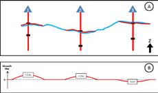
An interval velocity is the mean velocity between two horizons at a given XY location. Interval velocities are computed along each well. Figure 1A illustrates the concept with interval velocities computed for the shallow
unit between the ground (for onshore seismic) and the first key horizon HrzA, then for the unit A between HrzA and HrzB and lastly for the unit B between HrzB and HrzC. In a given unit, sonic shows that the velocity varies vertically. The interval velocity is an integration of these local vertical variations. Well tops are all we need to compute an interval velocity. The depth of top horizon and of the bottom horizon are known (by definition). As the well has been converted to time, the time two way-time (TWT) is known too. The interval velocity is the ratio between the delta-depth and the delta-TWT. If the interval velocity is more or less constant at each well, an average constant interval velocity might be assigned to the whole unit over the lease. This approach is also used when there are too few wells to interpolate the interval velocity on the map in any meaningful way. On the contrary, if we have enough wells and if the interval velocity varies from well to well, interpolation techniques are used to generate an interval velocity map between the well interval velocities. For every XY location, the interval velocity value from the map is then assigned to every point of the seismic cube at this coordinate. Having done this for each geological unit, the seismic cube can be converted to the depth domain with all the seismic interpretation. If only the seismic horizons need to be converted, it is done directly from the interval velocity maps.
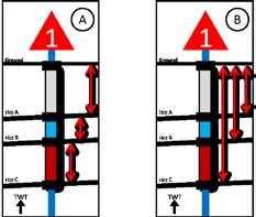
An average velocity is the mean velocity not between two horizons, as for the interval velocity, but between the ground and a given horizon (example, Figure 1B). Once the average velocity for a given horizon is known at each well, a map of average velocity is defined, either as a constant everywhere, or using interpolation techniques. The average velocity maps are then used to convert the seismic cube and/or interpretation to the depth domain.
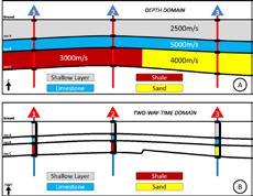
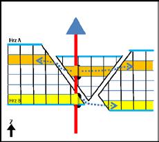
Interval velocities are preferred to average velocities for units with lateral changes of interval velocity (Figure 2). In this example,
the two first layers have more or less constant interval velocity of 2,500m/s and 5,000m/s respectively (Figure 2A) while the deepest layer has a sharp lateral change of interval velocity. The layer is a shale unit (3000m/s) truncated by a sand channel (4000m/s). Facies is one of the key factors to control the distribution of velocity in a geological unit. This lateral change of facies has an impact on the geometry of the seismic horizon of HrzC (Figure 2B). Where we are in the sand, the layer appears thinner, in the time domain, than where we are in the shale; while in the depth domain, the thickness changes smoothly between wells 2 and 3. In such a reservoir, it is essential to properly capture the limit between the zone where the wells have an interval velocity of more or less 3000m/s and are in the shale, to the zone where the wells are in the sand and show an interval velocity of 4000m/s. It means tracking the limit sand-shale between the wells and then to interpolate the interval velocities within each facies domain.
All these approaches of computing velocities at each well and then interpolating maps from them can also be done in a geomodeling package, if this is more convenient for the asset team to do so. Geostatistical algorithms, as introduced in the previous papers of this series, are perfect for interpolating the velocity maps. Not only to capture trends in the velocities, but also to generate multiple possible velocity maps, and so capture the velocity uncertainty between the wells.
No matter where these maps are generated, the geomodeler should make sure that these maps do include all the wells needed for the geomodeling workflow, and not only those used by geophysicist. In many projects, some wells might have facies and petrophysical logs, but they might not have a sonic log. Such wells would not be converted to the time domain by the geophysicist. It might be perfectly fine for seismic interpretation: once the time-converted wells have confirmed which seismic event shall be picked, the interpreter can follow these events in the whole cube, even around wells without a sonic log. The (... Continued on page 16)
Figure 1. Interval velocities (A) versus average velocities (B).
RESERVOIR ISSUE 11 • DECEMBER 2015 15
Figure 2. Reservoir with a lateral change of facies and velocity in the depth domain (A) and the time domain (B).
geophysicist might have the reflex, or be forced by his software, to create the velocity maps only from the time-converted wells. As a result, the depth-converted horizons, while fitting nicely to the wells with sonic, may not match to the wells without sonic. Such mismatches can be cleaned in the geomodeling workflow, as discussed in the next section, but it might be more elegant to create the velocity maps from all the wells in the first place, as well tops are all that is required to compute interval and average velocities. Sonic is not needed.
While illustrating the concept of lateral change of velocity, Figure 2 was also overly simplistic. In many reservoirs, the heterogeneity is such that facies do change both laterally and vertically, in very complex ways, and difficult to predict from wells. The velocities in such geological units might be better defined by creating geomodeling 3D-grid in the time-domain. A 3D facies model can then be built with geostatistical algorithms, and then the velocity can be modeled by facies. In such reservoirs, it might be necessary to interpolate sonic logs by facies instead of interval velocities, to really capture the heterogeneity. This geomodel will create multiple cubes of velocity for this unit, each one representing a possible distribution of the facies and the velocity in 3D. Overall, geomodeling packages are better equipped than geophysical packages to do such complex time-to-depth conversions.
SEISMIC INTERPRETATION AND STRATIGRAPHIC MODELING
When depth-converted seismic horizon data are available, the geomodeler must consider how to integrate the data into the model. He must create horizon surfaces which respect both the seismic interpretation and the well markers. Even when all the wells, with or without sonic, are used for time-todepth conversion, it is rare that the seismic interpretation matches precisely to the well markers. The reasons are many. The velocity maps might not have respected exactly the velocity value at each well. The time-depth conversion itself, once the velocity is modeled, might not have been exact either. This is not as rare as one might think. The reason might be also a question of timing in the team. Some well locations or some well KB elevation might have been adjusted after the depthconversion was done. Similarly, the geologist might have modified slightly the markers interpretation after the velocity maps were completed. At last, some wells might have been drilled after the seismic data got depthconverted. Or it might be a combination of all these events. In a perfect world, the geophysicist would systematically redo the
depth-conversion. But in many projects, the team might not have the time for that. The geophysicist might have been already assigned to some other tasks (or projects)...or the final deadline for the whole project might be too close to provide an opportunity to redo the depth-conversion.
If the mismatches are large, it is still recommended to adjust the velocity model and redo the depth-conversion. But if mismatches are reasonable, then they can be fixed directly in the geomodeling package.The technique, described hereafter, can probably be applied in many geophysical packages.
In Figure 3A, a seismic interpretation (blue line) has been depth-converted using the three wells 1, 2 and 3. The interpreted horizon is close to the well markers but a mismatch remains. Should it be corrected? A general rule in geomodeling is that if well data and seismic data are partly in contradiction, the well data shall be respected in priority because well data are more precise than seismic data. In the process of adjusting to the well, we try to respect the seismic data as much as possible. Naturally, if well and seismic data are in complete contradiction, it is wiser to understand ‘why’ instead of enforcing this rule blindly. Once the source of the inconsistency is identified, the team might agree that the data can be corrected to make them coherent one with the other, or the team might decide that the inconsistency is the result of different interpretations (for example). In that case, several geomodels might be needed, one for each interpretation. For the purposes of this section, we assume that it makes sense for our dataset to modify the seismic horizon to fit to the well markers.
One might be tempted to simply create a surface from the seismic interpretation and then adjust this map directly to the markers. By doing this, we mean using the depth of each marker to adjust the depth of the map. Such an approach might be risky. While the markers will be respected, it is also very likely that the whole surface will be completely smoothed out even far from the wells. The adjusted map might look very similar to the map we could generate from the markers alone. If it happens, at the least the team
needs to decide if that was the intention or if a different approach is needed. Creating a map showing the difference between the original and the corrected geometry is a nice way to understand how the geomodeling process modified the map exactly.
Instead of interpolating the depth values directly, we suggest another approach which better respects the geometry of the seismic interpretation: create a map of the adjustment you need to apply to the seismic horizon map (Figure 3A, blue line) to get it to fit to the markers. Then move the seismic horizon map with this adjustment map.
The first step of this workflow is to compute the mismatch between the original seismic map and each well marker. In our example (Figure 3A), the mismatch at well 1 is +1.2m, the mismatch at well 2 is +0.9m and the mismatch at well 3 is -0.6m. A negative number means that the marker is deeper than the surface at this location.We now know that the adjustment map must have the value +1.2, +0.9 and 0.6 at the respective XY locations of wells 1, 2 and 3 (Figure 3B). We also decide that the adjustment must be null past a certain distance from each well location. It means that outside of areas centered at each well, we don’t want to modify the original seismic map.
The second step of this workflow is to define the radius of these areas. More details will be given in a later paragraph. Once the radius defined, we know the displacement at each well and we know the displacement is 0m beyond the radius. All that remains to do is to use some interpolation technique to extrapolate a decreasing displacement from each well toward the limit of its associated area. On Figure 3B, it is illustrated by a bell shape around each well. Lastly, the displacement map is added to the original seismic horizon. The resulting, corrected horizon is equal to the original map far from the wells (= outside of the pre-defined radial zones around each wells) while the horizon has now changed around each well. Each marker is now respected while keeping the overall geometry of the seismic interpretation.
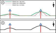
Figure 4. Effect of using different radius to compute the adjustment map. A) map resulting to three different radii (small, medium or large). B) map resulting from using at each well a radius function of the local mismatch.
(... Continued from page 15)
Figure 3. A) Original (blue) vs marker-adjusted (red) seismic interpretation. B) Adjustment map needed to correct the mismatch observed in (A).
16 RESERVOIR ISSUE 11 • DECEMBER 2015
As illustrated in Figure 4, the challenge is to decide what radius to use around each well. In this example, the mismatch at well A is half of the mismatch at well B. If we use a very small radius for both wells (Figure 4A, black thin line), the adjustment zone is really narrow and the corrected horizon surfaces might show an obvious bullseye around each well. Using a medium-size radius (Figure 4A, red dashed line), the bullseye effect might be less noticeable, and so acceptable, around well A, while it might still be too visible around well B. At last, using a large radius (Figure 4A, green thick line), the bullseye effect might now be minimal on both wells, but the question might become that we are altering a too large portion of the seismic maps around each well.
Ultimately, this is all a trade-off that the team must agree upon. If some mismatches are really too large or the bullseyes are too visible, then, as mentioned earlier, it might be wiser to redo the depth-conversion. An alternate approach might be to use different radii for each well (Figure 4B). The idea is to select a radius proportional to the absolute value of the mismatch: the more important the mismatch, the larger the radius. In Figure 4B, we could use a medium radius around well A and a large one around well B.
Once surfaces are created for each horizon on the well markers and a seismic interpretation exists, the geomodeler can continue taking advantage of the seismic interpretation in two ways, both illustrated in Figure 5.
Figure 5 is an extension of the example presented in Figure 4. Horizon A is the one for which a seismic interpretation existed, and got adjusted to the well markers at wells 1, 2 and 3. For the horizons B and C though, there is no seismic interpretation, only well markers.
In many reservoirs the horizons, or a subset of them, might be conformable, one with the other. If one of these conformable horizons has been picked on seismic, then it can be used as a reference to model the other horizons. In Figure 5, Horizon B is interpreted as conformable with Horizon A. We can use the geometry of the Horizon A to model the geometry of Horizon B. A thickness map of the unit between Horizon A and Horizon B is interpolated from the thickness at each well (using geostatistical algorithms). Then, the geometry of Horizon B is calculated by subtracting the thickness map to the depth map of Horizon A.This is a first additional way to take advantage of a seismic interpretation. Sometimes, none of the seismic events they can interpret correspond to any of the stratigraphic markers interpreted by the geologists on the wells.These events are linked to other change of log signatures along the
wells. When this happens, it is recommended to treat such horizon as we did here with Horizon A, and then create horizons for the real stratigraphic tops (= the horizons we do need for the 3D-grid) following the approach proposed here for Horizon B.
Other horizons known only from well markers are simply not conformable to any horizon picked on seismic. Such horizons can only be modeled from the well markers. No seismic horizon, such as Horizon A, can be used as a reference. In Figure 5, this is the case of Horizon C.
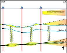
Another use of seismic interpretations is for quantifying the uncertainty on the geometry of the horizons. Horizons A, B and C illustrate different type of uncertainty geomodelers have to consider.
Horizon A is the best defined horizon as it was visible on seismic. There are still two sources of uncertainty though: uncertainty in the picking itself in the time domain and uncertainty in the depth-conversion (or depth migration as discussed at the beginning of the previous section).
Horizon B was created from Horizon A. As such, it inherits all Horizon A’s sources of uncertainty. An additional uncertainty must be considered too: the uncertainty on the thickness of the unit between Horizon A and Horizon B.
Horizon C, at last, is only known from well markers. As such, we have no real idea of how uncertain the interpolated surface is. Of course, mathematically, we can run different scenarios for this horizon, but which scenario bound to the uncertainty shall we use? +/5m? +/- 50m? More maybe? A solution is to define the range of uncertainty on Horizon C from Horizon A with the following approach.
Firstly, we create a new surface for Horizon A only from well markers. Such geometry is illustrated in a dashed blue line on Figure 5. We now have two geometries for Horizon A: the surface made from the seismic and the well markers and the geometry made
only from the well markers. The mismatch between the two maps tells us how incorrect – that is to say how uncertain – our map of Horizon A from the markers alone is. On Figure 5, the error is reasonable between the wells (yellow color), while it is very large to the east beyond well 3. One might assume that a similar range of uncertainty would have been found around Horizon C if it would have been possible to pick it on seismic. If we accept this assumption, we can simply assign the uncertainty map from Horizon A onto Horizon C (Figure 5, vertical thick arrows).
Many geomodeling packages have tools to create multiple versions of a given horizon, each version being a variation around a base case geometry. The tool is fed with an initial geometry of the horizon (Figure 5, the interpolated Horizon C map from the well markers) as well as an estimate of the range of uncertainty (Figure 5, the map of mismatches computed on Horizon A). Each variation is slightly different from the reference surface, but all surfaces fall within the range of uncertainty pre-defined by the uncertainty map. In Figure 5, a few possible variations of Horizon C are represented in thin dark lines.
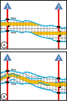
Figure 6. Reservoir in which the horizons are defined from seismic and from well tops. A) traditional approach to build the mesh of the 3D-grid (horizontal mesh). B) modern approach integrating local seismic events interpreted in the reservoir.
Up to this point, this section focused on integrating “traditional” seismic horizon interpretations. By “traditional”, we mean surfaces that can be picked across the whole seismic cube such as Horizon A on Figure 5. In the last few paragraphs of this section, we are considering the integration of the smaller
(... Continued on page
Figure 5. Modeling horizons from seismic interpretations and/or well markers and managing the uncertainty associated to the model.
18) RESERVOIR ISSUE 11 • DECEMBER 2015 17
seismic events that can be picked inside each geological unit.
In geomodeling, once the top and bottom horizons of a reservoir are modeled, we often create a 3D-grid with a mesh parallel to the top horizon, parallel to the base horizon or proportional between the two surfaces. If it seems more appropriate for the local geology, we can instead make the mesh horizontal (Figure 6A) or parallel to a surface other than the top and bottom horizons. In all these approaches, the seismic cube is not used to create the mesh, except when the reference surface the mesh is parallel to was itself picked on seismic.
This being said, as geomodelers, we should not forget that the internal heterogeneity of the reservoir might be partly visible on the seismic, in the form of local seismic events, that geophysicists can pick. A close collaboration between the geologist and the geophysicist might be needed there to ensure that those local, internal seismic events are coherent with the geological interpretation of the reservoir. If such local events are interpreted, it is in the team’s interest to see these local seismic events being used in the construction of the geomodel.
At the time this paper is written (autumn 2015), geomodeling packages start having tools to take these local events into account when creating the mesh of the 3D-grid. Figure 6B illustrates this concept as the mesh is following a few seismic events picked in the reservoir (thick blue lines between Horizon A and Horizon B). While such techniques are still not widespread, we think geomodelers should already start looking into this. Property modeling in a 3D-grid (facies and petrophysics) is primarily guided by the geometry of the 3D-grid itself. If we can add more “geology” into these meshes by using the local seismic events, we might improve the accuracy of our models.
SEISMIC INTERPRETATION AND STRUCTURAL MODELING
The technique presented in the previous section, to tie depth-converted seismic horizons to well markers, can be applied to adjust depth-converted seismic fault surfaces to fault markers. The remainder of this section provides an opportunity to discuss how geophysicists and geomodelers can collaborate to model a fault network through integration of seismic interpretation and geomodeling techniques.
In faulted reservoirs, only seismic data can really help defining the geometry of the faults and define how all these faults are interconnected to form the fault network. A
faulted geomodel is only as good as the seismic interpretation of the fault network, and how well this interpretation has been respected. In many projects, the workflow is a two-step process (Figure 7, “traditional workflow”). The geophysicist spends time creating and fine-tuning his interpretation of the fault network. Then, once the interpretation is finalized, it is transferred to the geomodeling package and the geomodeler creates the model. Building a faulted 3D-grid has been a tedious task in the geomodeling industry for years, partly because many packages were using an approach called pillar gridding. This technique is described later in this section as it is still used today. For complex fault networks, such geomodeling tasks can take a lot of time. In that context, a complex fault network would be one with many faults, maybe some faults dying in the reservoir or/ and some complex fault relationships such as Y-faults, X-faults. Because it takes time to build such model, it is often impossible to circle back with the geophysicist, even if building the geomodel highlights some inconsistency in the geophysical interpretation. There might simply be no more time left in the project to do these adjustments.
Over the last few years, some geomodeling packages have added more robust and simpler techniques to build quickly a fault 3D-grid. For the geomodelers having access to such modern workflows, it allows them to work with their geophysicist in a more integrated way (Figure 7, “integrated workflow”). The idea is for the geophysicist to provide a good, but not complete initial interpretation. The detailed cleaning, traditionally done to make life easier for the geomodeler, is not needed anymore. The geomodeler builds an initial structural model from this dataset, using the modern structural modeling workflows now available. The goal is to quickly get a 3D-grid which can be reviewed by the whole team. As for the traditional workflow, the review often leads to the need for further refinement of the geophysical interpretation and/or of the geomodel itself. But here, as the initial geophysical interpretation and the initial structural model were built fast, there is still time in the project for the geophysicist and the geomodeler to refine together the structural model.The final 3D-grid represents the reservoir more accurately. For this reason, we highly recommend using such modern approaches whenever available.
Considering that pillar gridding is still used a lot, more details are given hereafter (Figure 8). On the contrary, at the time this paper is written (autumn 2015) not all the details about these modern workflows have been made public yet by the different software companies. As such, a general idea of what
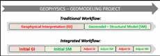
Figure 7. Geophysical and geomodeling project to build a fault network. The traditional workflow vs. a more modern, integrated one. The time spent on each task varies from project to project.
can be achieved with these techniques is illustrated in this section (Figure 9).
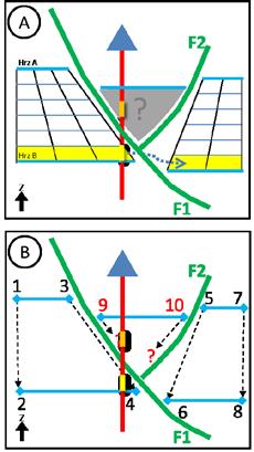
Figure 8A shows a faulted reservoir in which the faults F1 and F2 form a Y-fault network. The faults and the horizons A and B have been picked on seismic. The reservoir is also crossed by a well on which facies interpretation has been done (two facies zones are represented in orange and yellow). The 3D-grid represented on Figure 8A is typical of what a pillar gridding algorithm can generates. To the left of fault F1, the vertical mesh is parallel to the fault F1 near F1 and it progressively gets vertical when we reach the left limit of the modeled area. Similarly, the 3D-grid to the right of the fault F2, the mesh is parallel to the fault F2 and it gets progressively vertical the further away we are from it. Modeling the block between the faults is the challenging part. Most likely, and not represented here, the model would have been simplified to make it happen. The fault F2 will have been edited so as to remove the branching. Its geometry might have been altered to move the branching deeper, below
(... Continued from page 17) 18 RESERVOIR ISSUE 11 • DECEMBER 2015
Figure 8. A) 3D-grid of a Y-fault system modelled by pillar gridding. B) Details of the pillar gridding algorithm.
the modeled year. Another option could be to make F2 vertical and completely crossing the reservoir (fault dying in the reservoir are also an issue for the pillar gridding algorithm). In some project, the fault F2 might have been simply ignored and the throw it creates on the horizon A would be smoothed out. In all cases, very likely, the geometry of this fault network would have been altered.
Figure 8B explains in further detail why this is happening. The first step in pillar gridding is to connect each extremity of the top horizon to an extremity of the bottom horizon. By extremities, we mean points labelled 1, 3, 9, 10, 5 and 7 on Horizon A and the points 2, 4, 6 and 8 on Horizon B. Point 1 from Horizon A is connected to point 2 of Horizon B because they correspond to the left extremity of the input horizons. Point 3 from Horizon A and Point 4 from Horizon B are connected because they both represent the point of contact between the horizon and the fault F1 on the left fault block. Using a similar approach, the points 5 and 6 are connected as well as the point 7 and 8. But what shall we do with the extremities 9 and 10 on Horizon A? As the block between the two faults doesn’t extend to Horizon B, there is no extremity on Horizon B to associate them to. And that’s where the pillar gridding algorithm is blocked. Simplifying the geometry of Fault F2 is the trick used to make sure we have as many extremities on Horizon A that we have on Horizon B. Once it’s done and all the extremities are connected, the vertical mesh is further defined inside each block so as to make a smooth transition between one connection to the next one. At last, the horizontal geometry to the mesh is added.
model is sealed has always been one of these issues. By sealed, we mean that there must be no gap between the horizon surfaces and the fault surfaces where the former gets in contact on the later. The gap visible on Figure 8 and Figure 9 between the horizon and the fault surfaces were added only to give more clarity to the pictures.
Secondly, these new workflows try to ensure that there no need to simplify the fault network anymore. It means that they don’t rely on pillar gridding algorithms. Figure 9 is an example of the type of output 3D-grid we can get. The fault block between F1 and F2 is now properly managed. Observe also how the cells of the 3D-grid are now cut by the two faults instead of being parallel to them (Figure 8). This is also an improvement as conceptually, one has to imagine that rocks got deposited before they got faulted (except around growth faults). As such, it makes sense that our facies distribution gets “cut” as in Figure 9 instead of getting aligned to the fault as in Figure 8.
As for the integration of local seismic events, described at the end of the previous section, these modern structural modeling techniques have both challenges and benefits. Challenges, because they are still new and use geomodels and we are not yet used to them. But beneficial too, as some complex reservoirs, when applied correctly, might be the key to building a really good geomodel.
GUIDING PROPERTY
MODELING WITH SEISMIC DATA
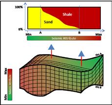
A seismic cube can contain a lot of useful information to guide 3D facies modeling and 3D petrophysical modeling. Geophysicists, for decades, have been developing many techniques to correlate signature in the seismic cube to specific facies or log signature along the well. The general goal is to identify a signature in the seismic cube at the well location and to track such signature between the wells, assuming that wells drilled there would see the same log/ facies signature than observed on the existing wells. The purpose of the present paper is not to detail all these geophysical techniques – it would be impossible. The reader can refer to books such as (Chopra and Castagna, 2014), (Li, 2014) and (Simm and Bacon, 2014) for some introduction on the topic. Our goal here is to see, once the geophysicist has created one or several new seismic attributes, how shall we use them in our geomodeling workflows?
and, as explained hereafter, all these seismic attributes are integrated in the geomodel using a limited set of techniques too.
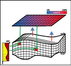
Error! Reference source not found. illustrates how a continuous seismic attribute can be transformed into a set of cubes of facies probabilities. Along each well, the facies distribution is compared with the values of the seismic attribute (Error! Reference source not found., upper part). In our example, one can see that for values of the attributes up to A, the facies on the well is always sand.We can assume that between the wells, everywhere where the attribute is in that range, we will have always sand. In these cells, the cube of sand probability is equal to 100%, while the cube of shale probability is equal to 0%. In a symmetric way, for values above B, the facies at the well is always shale. In the cells with this range of values, the cube of sand probability is equal to 0% and the cube of shale probability is equal to 100%.
The new structural modeling workflows developed over the last few years seem to focus on two things.
Firstly, they automate a lot of the tedious tasks usually done manually in older workflow. These tasks are not described in any details here, except to say that ensuring that the
On a geomodeling point of view, seismic attributes and petrophysics are similar. You can have numerous seismic attributes in the same way that as you can have many different types of logs to model in 3D. But at the end of the day, all these logs are modeled using a limited set of geomodeling techniques
If this binary behavior (either 100% chance to be in sand or 100% chance to be in shale) was true for all values of the seismic attribute, we wouldn’t even need any geostatistical computation. For a given cube of seismic attribute, the facies distribution would be purely deterministic. It would mean that the seismic attribute on its own would be enough to characterize the reservoir. In practice though, the relationship is never as clear as this and there is always at least range of values for which there is probability to be either in the sand or in the shale. This is where geomodeling and geostatistics find its place: it allows throwing the dices and generating multiple facies realizations which respect that information. Concretely, for each attribute value between A and B (Error! Reference source not found., upper part) we assign the proper probability in the sand and the shale cubes.
This illustrates what was discussed in the introduction of this paper. Seismic cubes
Figure 9. Example of 3D-grid built with more modern structural modeling techniques, that don’t rely on pillar gridding algorithms.
Figure 10. Cube of facies probability built from combining a VPC and a facies proportion map.
RESERVOIR ISSUE 11 • DECEMBER 2015 19
(... Continued on page 20)
can’t see the reservoir at the resolution that wells can. As such, seismic attributes can’t capture the details and there are always some discrepancies between the seismic information and the well information. Geostatistics, through the use of cube of facies probability, allows studying this uncertainty. The same approach would work if the seismic attribute was a discrete property.
As mentioned earlier, several attributes might have been computed. Each attribute will generate its set of probability cubes. If multiple sands and shale probability cubes exist, they can be combined into an integrated single cube. The same can be done to merge together a set of cubes coming from seismic and the set of cubes generated from merging VPC and facies proportion maps. The idea is that each cube, each data, shows one aspect of the facies distribution and to understand the whole distribution, we need to combine them.
If a seismic attribute relates to a continuous well log such as porosity, or fracture density, the seismic attribute is directly used as a secondary variable with geostatistical algorithms such as Collocated Sequential Gaussian Simulation (collocated SGS). The workflow is identical to the one described in the paper on petrophysics where the 3D
porosity model was used as a guide to model the water saturation in 3D. Such algorithms are able to use multiple secondary variables if needs be.
The reader can refer for example to (Doyen, 2007) for more details about these different techniques.
CONCLUSION
Geophysical data are an essential part of any geomodeling workflow and reciprocally, geomodeling techniques can complement generating certain geophysical results as well as get the most out of the different types of geophysical interpretation.
The most common mistake is to assume that seismic is only useful for guiding horizon and fault modeling. A lot of information about the reservoir characteristics can also be extracted from a 3D seismic cube. Once this accepted, a proper collaboration between the geophysicist, the geomodeler and the other team members will allow for the best integration possible.
TO GO BEYOND
As part of its training program, the CSPG offers a course on geophysics. Beyond that, those interested in these topics shall also look at the excellent training program organized also yearly by the CSEG (Canadian Society of Exploration Geophysicists), as well as to the presentations that they organize and the magazine that they publish.
ACKNOWLEDGEMENT
The authors would like to thank Maximo Rodriguez, Senior Geophyscist at ConocoPhillips Canada, and Junaid Khan, Senior Geophysicist in Husky
REFERENCES
Al-Chalabi, M., 2014. Principles of Seismic Velocities and Time-to-Depth Conversion. EAGE Publications. 488 pages.
Chopra, S. and Castagna, J.P., 2014. AVO. SEG. 288 pages.
Doyen, P.M., 2007. Seismic Reservoir Characterization. An Earth Modelling Perspective. EAGE Publications. 255 pages.
Jones, I. F., 2010. An Introduction to: Velocity Model Building. EAGE Publications. 295 pages.
Li., M., 2014. Geophysical Exploration Technology. Applications in Lithological and Stratigraphic Reservoirs. Elsevier. 449 pages.
Simm, R. and Bacon, M., 2014. Seismic Amplitude. An Interpreter’s Handbook. Cambridge University Press. 271 pages.
THE AUTHORS
Feel free to contact the authors about this paper or about the series.
Thomas Jerome is the Calgary manager of the Reservoir Modeling team in RPS (Thomas.Jerome@rpsgroup.com). Geologist by background, Thomas has spent the last 15 years working on geomodeling projects, first in Middle-East and in Calgary, Canada, since 2008. He has worked on conventional and unconventional reservoirs, both Canadian and international. Thomas is leading this CSPG’s series on Geomodeling.
Sher Ali is Senior Geomodeller with Brion Energy Corporation at Calgary (Sher.Ali@ Brionenergy.com). Sher started his career from Asia and worked in Africa and Middle East before moving to Calgary, Canada in 2011.
Nilanjan Ganguly is a Senior Geophysicist with Canacol Energy Ltd (nganguly@ canacolenergy.com). Nilanjan received his B. Sc. degree in Geological Sciences from Indian Institute of Technology and M. Sc. in Geophysics from University of Victoria. For the past 16 years, Nilanjan has worked on various international and frontier basins: primarily in Africa, Middle East and South America. His professional interests include exploration in highly structured areas, AVO, seismic attributes and inversion.
(... Continued from page 19) Many CSPG memberships expire December 31st. Watch your email for a link to renew online. **membership is on an individual basis; you may have a different expiry date** 20 RESERVOIR ISSUE 11 • DECEMBER 2015
Figure 11. Combining well facies and a seismic attribute to create a set of cubes of facies probability.
ANNUAL YOUNG GEOSCIENTISTS NETWORKING RECEPTION
| By Denise Yee, 2015 Young Geoscientists Networking Reception Chair
The 6th Annual Geoscientists Networking Reception took place on October 29th, 2015 at The Garage Sports Pub in Eau Claire. With 100 attendees, both inexperienced and senior geologists enjoyed a few drinks while getting the opportunity to network with each other.
The annual event is held to help bridge the gap between experienced and new-to-the industry geoscientists. The reception is an informal way for communication of stories, tips and tricks of the oil and gas industry to get passed down to the younger generation. The exposure to mentorship opportunities and CSPG involvement options are two major reasons for attendance. If you have any ideas for such events or would like to volunteer for a position on the newly formed Young Professionals Committee, please contact Ryan Lemiski at ypg@cspg.org.
CSPG thanks the volunteer committee and our generous sponsors for the event; Chinook Consulting (Booth Sponsor), ITG Investment Research (Booth Sponsor) and Crescent Point Energy Trust (Gold Sponsor).

Thank-you to our sponsors!


Thank-you for supporting CSPG initiatives

Calling all Young Geoscientists! Join us for our Christmas Social and Technical Luncheon on December 8th at the TELUS Convention Centre The CSPG is inviting you to take part in a new initiative at our Technical Luncheons. It will provide an opportunity for young professionals to network with senior geoscience mentors, enjoy a quality technical presentation, and gain valuable APEGA PDH at a reserved table! Go to www.cspg.org/ypg to register and find out about more about the new initiatives focused on Young Professionals!
RESERVOIR ISSUE 11 • DECEMBER 2015 21
GUSSOW CONFERENCE 2015
Fine Grained Clastics: Resources to Reserves
Meeting Summary
On a cool winter’s eve earlier this year, a professor, a philosopher and a wizard entered the castle of one of our society’s past royalty (executive). There, under the influence of thin crust pizza and a few beverages, the concept for Gussow 2015 was created.
The goal to inform and educate this year’s Gussow delegates using the theme of taking unconventional fine-grained reservoirs from resources to reserves was the task at hand and the flow of the conference was constructed to follow this format. With over 85 G&G and Engineering attendees hearing 34 papers over the two and a half day event, the agenda proceeded from setting the foundation based on rocks and fluids, to tools required to build the plays, to getting value as a reserve or marketable product and then to reviewing case studies was well received.
Sessions were held in the Max Bell building at the Banff Centre from October 13-15th with presentations evenly split between representatives from academia, industry and service companies. Of note, Roger M. Slatt visited from the University of Oklahoma and Stephen A. Sonnenberg joined proceedings from the Colorado School of Mines. Postconference training was offered in downtown Calgary by Steve Sonnenberg on October 16th (Unconventional Oil).
Some, but not all, of the highlights and takeaways were:
Frank Stoakes on Swan Hills carbonates: “You don’t need geophysics, you need core!”
JP Zonnenveld on the Triassic: “The Montney basin is similar to an upside down Sea of Japan”
Roger Slatt on the incised valley Woodford shale play”: “...drill in the lows.”
Steve Sonneberg’s Wattenberg Field: “ one of the largest in the USA and still growing production”
Ken Ratcliffe: “ ... you need to stay in your reservoir while drilling horizontally.”
Dave Eaton on Microseismic facies analysis: “ ... parent and child events for more detailed analysis.”
Natalia Verkhovtseva on improving completions “ ...using downhole microseismic and tilt-meters.”
Dan Potocki’s DFIT analysis on wells throughout the planet
Tyler Schlosser on assessing Value: “...68% confidence the price will be between $32 and $75/bbl in 2016”
Sheila Legget’s public consultation: “...guide posts for the right thing to do”.
Tuesday evening wrapped up with an outdoor presentation by Paul McKay on the geology of the mountain ranges that can be summed up by “... all you need to remember is ‘PBR’, Palliser, Banff then Rundle!”
The Wednesday evening dinner Keynote address by Raffi Tahmazian of Canoe Financial gave us a very educational and engaging Energy Update. “...we are
cautiously optimistic that we may have turned the corner...”
It was a great conference with tremendous learning’s and good conversation; it became clear that it is necessary to fully understand the rocks, push the envelope on technology and focus on economic results.
Special thanks go out to the CSPG staff, Candace Jones and Lis Bjeld, Mark Caplan and Paul McKay of the CSPG executive, and the Banff Centre. Thank you to all attendees, speakers and poster presenters. Also, a large thank you to our event sponsors: Long Run Exploration, APEGA, Paradigm and AGAT Laboratories.
 Gussow Co-Chairs: (left to right)
Rob Galant, P.Geo. “The Philosopher”
John LJ Duhault, P.Geoph. “The Wizard”
Per Kent Pedersen, P.Geo. “The Professor”
Gussow Co-Chairs: (left to right)
Rob Galant, P.Geo. “The Philosopher”
John LJ Duhault, P.Geoph. “The Wizard”
Per Kent Pedersen, P.Geo. “The Professor”
22 RESERVOIR ISSUE 11 • DECEMBER 2015
Group photo of the participants at the Gussow Conference

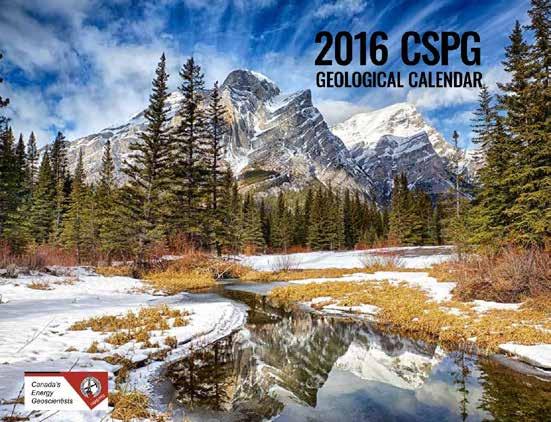
Available NOW for 10 dollars! Office: 110-333, 5th Ave SW Phone: 403.264.5610 Start your year off right with the 2016 Geological Calendar RESERVOIR ISSUE 11 • DECEMBER 2015 23
Save the Date The prestigious AAPG 2016 Annual Convention & Exhibition (ACE) returns to Calgary for the first time in a decade. Join the world's best and brightest geoscientists and energy leaders at this premier industry event. Exhibition and Sponsorship Opportunities Available. ACE.AAPG.org 24 RESERVOIR ISSUE 11 • DECEMBER 2015


elizabeth macey, B.A., cartographer . 993. 0055 emacey@telus.net www3.telus.net/elizabethmacey . . presentations posters graphics . maps technical illustrations RESERVOIR ISSUE 02 • FEBRUARY 2015 9 • Domestic and International wellsite supervision • Conventional and Unconventional wells • Extensive Hz experience • Customized corporate solutions available (403) 250-3982 sales@clconsultants.ca www.clconsultants.ca Wellsite Geologists Inc. the Rock Solid Choice Wellsite Supervision Project Management Graphic Well Profiles Verticals / Horizontals EUB Sample / Core Studies Conventional / Un-conventional 1350, 734 - 7th Ave SW Calgary, AB T2P 3P8 B 403.234.7625, www.WellsiteGeologists.com C 403.660.9883, info@WellsiteGeologists.com 1602 – 5th St N.E. Calgary, AB. T2E 7W3 Phone: 403-233-7729 www.tihconsulting.com e-mail: tih@shaw.ca T.I.H. Consulting Ltd. Geologic Well-Site Supervision
CORPORATE SUPPORTERS
Paramount Resources
CMC Research Institutes, Inc.
Big Guns Energy Services
Earth Signal Processing Ltd.
Pason System
Roke Technologies Ltd.
Canada Brokerlink Inc.
ITG Investment Research
Nalcor Energy
Lee Energy Systems
NExT- A Schlumberger Company
Compass Directional Services
EV Cam Canada Inc.
Valeura Energy
Birchcliff Energy Ltd.
Sproule Associates Limited
Waterline Resources
Cabra Consulting Ltd.
McDaniel & Associates Consultants Ltd.
National Oilwell Varco
Signature Seismic Processing Inc.
Navigator Resource Consulting
Pulse Seismic Inc
Richardson GMP
Surge Energy Inc.
Statoil Canada
Mundiregina Resources Canada
Mcleay Geological Consultants Ltd.
Enviro-Tech Surveys Ltd
Tucker Energy Services Canada
Bounty Developments Ltd.
Franconia Geoscience
GeoChemTech Inc.
Prospect Drivers Inc.
RPS Energy Canada Ltd.
AS OF OCTOBER 30, 2015
HONORARY MEMBER Graeme Bloy

Graeme Bloy completed his Honors B.Sc. and M.Sc. at the University of Alberta, the first in 1975, and the second in 1979 with a thesis on Geochronology of Uranium Mineralization in the East Arm of Great Slave Lake. Graeme joined the CSPG in 1978 and his first committee in 1981: the Manpower Survey Committee, where he served for three years. Then he served for five years on the Education Committee, earning himself a Service Award in 1991. He was Co-Chair of Technical Sessions for the 1994 CSPG-CWLS convention. Mr. Bloy was the Educational Trust Fund Chair from 2000 to 2005, and earned a Service Award during that time. His three year Executive term centred around his 2009 Presidential year, where he focused on reorganizing the office and conferences, and growing the Educational Trust Fund. He also served on the President’s Award Committee and the Compensation and Benefits Committee while on the Executive. He earned a H. M. Hunter Award 2012, and then joined that Committee to honor others. From the late 1980s through 2005, Graeme co-lead CSPG field seminars and co-organized several CSPG short courses on carbonate deposition and reservoir characterization and fractured carbonate reservoirs.
As well as the CSPG, Graeme is a member of AAPG, SEPM and APEGA. He is active in the Roman Catholic Diocese of Calgary and is a Master’s swimmer.
Graeme started his career as a Geologist for Hudson’s Bay Oil & Gas, followed by positions at BP Canada, ThomsonJensen Petroleum and Husky Oil. In 1996, he became the Staff Geologist at Startech Energy, a role he held for two years, and accelerated development of acquisitions through infill and horizontal drilling. Next he moved to Devon as an Exploration Manager, where he used his expertise in carbonate rocks and fractured carbonates to define reservoir predictability and quality assessment; mentored and trained junior geologists; and managed a 75 well per year drilling program. In 2007, Mr. Bloy moved to West Energy as the Vice President of Exploration, a role he held for two years, before moving to Canada Capital Energy as the Vice President of GeoSciences, where he was responsible for the startup of private Chinese–funded oil company based in SE Saskatchewan. Since 2013, Mr. Bloy has been the President of Atum Consulting and Quarterpoint Resources. He provides geoscience expertise, assists in a geoscience management role, and acts as a geoscience advisor to external senior management teams and Board of Directors for issues concerning strategies for growth, divestiture or investment.
Graeme’s role as a mentor cannot be understated. He is clearly dedicated to spotting talent and doing what it takes to nurture and grow individuals. His willingness to donate his knowledge, time and unbridled passion for our science is well known, and very much appreciated by all who work with him.
Graeme Bloy has been a geoscientist for more than 35 years, as well as an entrepreneur, a mentor and an outstanding volunteer. His wide range of experience brings a phenomenal knowledge base to any team in which he works or leads, and his commitment to the advancement of science has bettered both the companies he has worked for and the industry at large. The CSPG is pleased to welcome Graeme Bloy in to the ranks of Honorary Membership.
26 RESERVOIR ISSUE 11 • DECEMBER 2015
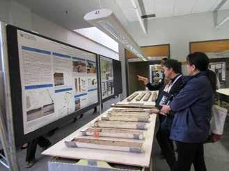
The vision and goal of the Canadian Society of Petroleum Geologists (CSPG) is to make the Core Conference the signature post-session of the AAPG 2016 Annual Convention & Exhibition (ACE), being hosted in Calgary, Alberta, Canada . The theme for the 2016 International Core Conference, "Redefining Reservoir: Core Values”, will reflect the key geologic value we all share: the rocks tell the most important stories in our hydrocarbon quests!
2016 INTERNATIONAL CORE CONFERENCE
Dates: June 23rd-24th, 2016
Time: Thursday: 8 AM to 4 PM
Friday: 8 AM to 3 PM - CoreMeltdowntoFollow
Location: AER Core Research Centre
3545 Research Way NW, Calgary, AB, Canada
Fee: $195 US (includesCoreMeltdownticket)
$25 US for Core Meltdown only

If you haven’t been to a Core Conference before, you are in for a treat! The conference will be held in the world-class AER Core Research Centre that will accommodate over 30 core displays and accompanying posters over the two-day event. Exhibitors provide scheduled talks summarizing their displays and remain with their core to discuss concepts and features. This year we will host cores from all over the globe – Turkey, Brazil, Germany, and North America. Displays will include both conventional and unconventional plays; siliciclastics, carbonates and evaporates, shales, oil sands, as well as some displays relating to carbon capture technology. We hope you will extend your stay in Calgary to attend this two-day post-ACE Core Conference on June 23rd and 24th, 2016!

CORE MELTDOWN 2016 AGAT Rocky Mountain Saloon
Don’t miss out on the tradition – join us for the Core Meltdown at this year’s AGAT Rocky Mountain Saloon. After two days of technical discussion and demonstration, come enjoy Calgary’s Western Heritage at our rain or shine tent event. Live music, food, and beverages make this event the perfect way to finish off the week. Admission and two drink tickets are included in the conference fee. Tickets for the Core Meltdown only may also be purchased separately. Hope to see all you cowboys and cowgirls there!

RESERVOIR ISSUE 11 • DECEMBER 2015 27
Help influence the governing of your profession
For the first time in more than 30 years, we’re reviewing the Engineering and Geoscience Professions Act to ensure it continues protecting the public interest while reflecting modern industry business practices.
A lot has changed over the years, and APEGA needs to be governed by legislation that gives us the authority and tools to regulate geoscience in today’s world.
Reviewing the legislation is a complex and lengthy process, starting with the Act, followed by the Regulations, and then the Bylaws. We anticipate it will take until spring 2019 to complete.
If you haven’t already participated in any of the consultations, you will have more opportunities in 2016 to provide your feedback and shape the future of the geoscience profession.

For more information and updates, please visit: www.apegalegislativereview.ca
