Wildlife Habitat Connectivity in Whatcom County, Washington

E x e c utive Su m ma r y

Wildlife habitat connectivity is crucial for the survival and well-being of many wildlife species, especially where human development has fragmented the natural landscape. Whatcom County, Washington has recognized the importance of preserving wildlife habitat connectivity alongside other critical areas such as wildlife habitat conservation areas, fish habitat conservation areas, and wetlands. However, Whatcom County has not yet formally identified critical areas for wildlife habitat connectivity conservation areas within the County’s geography.

This report by Wildlands Network describes a novel set of geospatial connectivity analyses that provide information about the current state of wildlife habitat connectivity in Whatcom County. We used multiple, complementary modeling methods to identify the largest remaining patches of wildlife habitat, the best connections between those habitats, the most likely migration paths for terrestrial wildlife, and the relative value of each part of the landscape for supporting wildlife habitat connectivity.

This information is intended to support Whatcom County’s efforts to identify important areas for wildlife habitat connectivity and designate critical connectivity areas for consideration under the County’s Critical Area Ordinance. These critical connectivity areas could help highlight important habitat connections in need of conservation, identify fragmented areas where habitat restoration could improve connectivity, and guide future development to areas where it would have the least negative impact on connectivity. We hope the greater conservation community will also use these maps to support their work to protect wildlife across Whatcom County and the surrounding landscape.

Black-tailed deer.

Photo: Cavan

Wildlife habitat connectivity – the ability of a landscape to facilitate the movement of wildlife species across it – is critical for wildlife to thrive and ecosystems to function. Animals move to find resources, migrate across seasons, avoid dangerous disturbances, or find new mates and habitats. Even stationary species like plants and fungi move across generations as habitats shift and environments change. The ability to move through a connected landscape with intact habitat and limited human impact is necessary for many species to survive, thrive, and evolve. This is especially true in the face of the growing impacts of climate change, which will cause species’ ranges to shift. Fortunately, awareness of the importance of wildlife habitat connectivity and corresponding efforts to conserve and restore it are on the rise around the world.

Whatcom County, Washington has recognized the importance of wildlife habitat connectivity and identified the need for a connectivity analysis of their geographic area. The Critical Area Assistance Handbook recommended identifying and designating any lands essential for habitat connectivity (Ousley et al. 2003). Another report for the Whatcom County Critical Areas Ordinance noted that “Washington State Growth Management Act guidelines suggested that ‘Land essential for preserving connections between habitat blocks and open space’ be one of the identified habitat types to be designated as a fish and wildlife habitat conservation area” (Whatcom County Planning and Development Services, 2005). Despite these recommendations, Whatcom County has not yet identified critical areas for wildlife habitat connectivity.

Locating these critical areas will inform development planning under Whatcom County’s Critical Area Regulations, which include a stated goal to “maintain the natural geographic distribution, connectivity, and quality of fish and wildlife habitat and ensure no net loss of such important habitats” (Whatcom County Planning and Development Services, 2017). Critical Connectivity Areas should be considered alongside previously mapped features like Wildlife Habitat Conservation Areas (including streams), Floodplains and Frequently Flooded Areas, and wetlands during Critical Area Regulation reviews. In addition, maps of wildlife habitat connectivity in Whatcom County could support and inform local conservation and restoration efforts through the County’s Conservation Easement Program and other County and partner conservation programs. These maps could also guide implementation of the State Wildlife Action Plan, which is currently under revision. While several large-scale connectivity maps have been developed for the United States, none offer the level of local detail and resolution necessary for recognizing critical connectivity areas in the developing and actively managed areas of Whatcom County (McRae et al. 2016, Theobald et al. 2011, Belote et al. 2016, Barnett and Belote 2021). So, the Whatcom County Planning Department’s Natural Resources Division reached out to the Wildlands Network to support development of a connectivity map specifically for the County.

Wildlands Network is a non-profit conservation organization that seeks to reconnect, restore, and rewild North America for the benefit of all life. We are a science-driven organization

Figure 1. Whatcom County, Washington, the Whatcom County jurisdictional boundary, and the management status of protected lands.

specializing in connectivity analysis, conservation, and policy whose founders were among the vanguard of conservation ecology and connectivity science (e.g. Michael Soulé, considered one of the founders of conservation biology, John Davis, and Reed Noss). Whatcom County asked Wildlands Network to analyze and visualize the current state of wildlife habitat connectivity in the County to help identify critical connectivity areas, increase conservation and restoration of connectivity, and guide development in the county to maintain ecosystem connectivity and minimize connectivity loss.

Whatcom County is situated in the northwestern corner of Washington State between Skagit County to the south, Okanogan County to the east, British Columbia to the north, and the Salish Sea (Puget Sound) to the west. The actual jurisdictional area of Whatcom County covered by the Critical Area Ordinance – not including other municipalities, federal land, and tribal nations – covers less than half of the land area of the county proper (Figure 1). This jurisdictional boundary contains the bulk of the county’s urban development, human population, major roads, and working lands (including agriculture and forest lands), all of which contribute to fragmentation of wildlife habitat and loss of connectivity. The land here includes coastal lowlands, abundant wetland and riparian areas, rich valleys, and mountainous foothills. The

eastern part of the county, dominated by the Cascade Mountain Range that runs south-to-north through Washington into Canada, is almost entirely federally owned and managed by the U.S. Forest Service or the National Park Service.

Although this connectivity analysis was designed to serve Whatcom County, we expanded our study area beyond the County borders. This was both because we did not want edge effects at the county line (due to the analysis not incorporating information about the land outside it) and because to wildlife and ecosystems, these borders are mostly arbitrary. Instead, we decided to define our study area as the combined area of three of Washington’s Water Resource Inventory Areas (WRIAs 1, 3, and 4). These management units are defined by major drainage basins including the Nooksack basin, the Upper and Lower Skagit basins, the Sumas River basin, the Sauk basin, and the Strait of Georgia basin. Their combined area covers all of Whatcom County, most of Skagit County to the south, some of Snohomish County, and part of British Columbia to the north (Figure 2). Using this expanded study area allowed us to create maps that look beyond the borders of Whatcom County, are more relevant to current landscape management scales (the WRIAs), and are ecologically meaningful.

Figure 2. The project study area was defined by the watersheds that make up Water Resource Inventory Areas 1, 3, and 4.

An Overview of Wildlife Habitat Connectivity Modeling

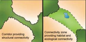
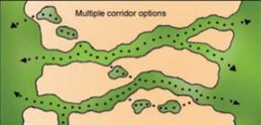
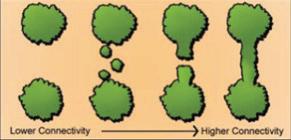
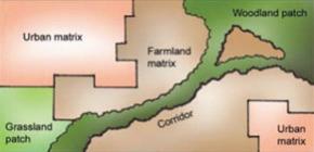
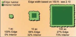
Wildlife habitat connectivity describes the degree to which wildlife species can move across a landscape to access the habitat and resources they need to survive. In a fragmented landscape, suitable habitat is often isolated in patches surrounded by unsuitable habitat, like islands in an ocean; larger patches are more valuable because they have more interior area that can be used as habitat (Figure 3A). For example, in a developing area like western Whatcom County, forest-dwelling species may be limited to patches of forest surrounded by a matrix of urban, agricultural, and less suitable natural lands (Figure 3B). Connectivity between these patches in the form of permeable landscape, stepping stone habitat patches, or connected habitat corridors allows those species to move between habitat and supports the survival of the species overall (Figure 3C). These important habitat connections should allow multiple movement routes through a relatively permeable landscape (Figure 3D). And ideally, a connection between core habitat patches should be wide enough and suitable enough to act as intermediate species habitat in its own right (Figure 3E). Using multiple strategies to increase landscape permeability and movement pathways between core habitat patches is essential for maintaining wildlife habitat connectivity on the landscape level.

There are many ways to model wildlife habitat connectivity, from single-species models based on animal movement data to general landscape models for large groups of species. Since our mission was to provide a broad overview of connectivity in Whatcom County, we chose a structural landscape approach. Structural connectivity models, unlike species-specific models, use information about the landscape itself –including proxy variables related to naturalness, human landscape modification, or mortality risk – to create a generalized, species-agnostic model of wildlife habitat connectivity. Previous research, including some in Washington and the Columbia Plateau, has shown structural connectivity modeling to be a robust alternative to species-specific models that offers comparable insight into wildlife habitat connectivity with fewer data and analytical requirements (Marrec 2020, Krosby 2015).

The biggest limitation to this broad approach is that it cannot and does not accurately capture habitat connectivity for all wildlife due to the various needs of different species. Most importantly, our connectivity models are limited to terrestrial wildlife and do not reflect the network of habitats used by most aquatic species. But even among terrestrial wildlife, certain

Figure 3. Wildlife habitat connectivity in a fragmented landscape depends on the configuration of habitat patches and connecting corridors through a matrix of less suitable lands (Figures from Bentrup 2008).

landscape features may facilitate or inhibit the movement of some species and not others. For example, a major highway poses a deadly barrier to animals that move on foot, but might have very little impact on the movement of many bird species. When creating a connectivity model, we must decide what to include as barriers to movement, and that brings with it certain assumptions about the species to which that model best applies. The connectivity models described in this report best reflect the needs of terrestrial species that: 1) avoid human development when possible, 2) avoid roads and/or risk mortality by crossing them, 3) avoid traversing steep slopes when possible, 4) cannot easily cross large bodies of water, and 5) prefer habitat consisting of unfragmented natural landcover in patches of 100 acres or larger.

We used two connectivity analysis methods to provide a more complete picture of connectivity in Whatcom County.

The first, Linkage Mapper, is a widely-used suite of connectivity tools that can be used to map wildlife linkages and corridors between core areas of habitat (McRae and Kavanagh 2011). The second, Omniscape, uses circuit theory to simulate wildlife movement across the entire landscape without defined habitat cores (Landau 2021).

Finally, we created a Connectivity Value index to summarize how much each part of the landscape contributes to wildlife habitat connectivity. This index combines the results of the analyses in this report with other connectivity data including Wildlands Network’s Pacific Climate and Non-Climate Connectivity Maps, created in partnership with the University of Washington (Nuñez et al. 2022).

Creating the landscape resistance layer Methods

Before conducting connectivity analyses using Linkage Mapper and Omniscape, we needed to create a landscape resistance data layer. Landscape resistance is a metric that represents the relative difficulty and/or risk to wildlife moving across a landscape due to characteristics of that landscape. This metric is often expressed as “cost distance.” Every piece of land that an animal must cross has some cost to the animal. This can mean the literal calorie cost of traversing that land or the relative risk of death from predation, hunting, vehicle collisions, and other natural or human causes. For example, it is generally much safer and easier for an animal to move through its preferred habitat in a remote area than to traverse the same distance across a human-populated landscape with dangerous roads. Creating a landscape resistance layer is an attempt to calculate the relative cost to

wildlife moving through a landscape, here represented as 30-by-30-meter cells in a raster grid.

There are many ways to calculate landscape resistance ranging from structural resistance based on landcover type to localized, species-specific resistance generated from actual animal movement data. Since the purpose of this project was to give a broad overview of structural connectivity for all terrestrial wildlife, we used a general approach based on detailed landcover and dispersal barriers like roads. This approach was partially modeled after a recent connectivity modeling project in southwestern Washington completed for the Washington Wildlife Habitat Connectivity Working Group (Gallo et al. 2019).

Whatcom Falls. Photo: Paula Cobleigh

For landcover information, we used the Ecological Systems of Washington in the U.S. (WDNR 2019) and 2015 Landcover of Canada in British Columbia (Natural Resources Canada 2015). The Ecological Systems of Washington is a 30-by-30-meter cell raster layer based on the U.S. National Land Cover Database (NLCD), but it includes many more land cover categories for specific ecosystem types (like “Northern Rocky Mountain Western Larch Savannah”) and human disturbance (like “Quarry, Mines, and Gravel Pits”). The 2015 Landcover of Canada is the same resolution (30-by-30-meters), but the categories are significantly less detailed, containing only general types of natural community and only one class for “urban and built-up” areas. Each landcover class was assigned a score from 1 to 1000, where 1 represents the least resistance to wildlife movement. In general, we borrowed these scores from Gallo et al. (2019), but because we used different landcover datasets, some scores had to be added or adjusted. A full list of the landcover types and the scores assigned to them can be found in

Fragmenting features such as roads impose significant additional costs to landscape connectivity, both due to physical risk to wildlife and avoidance of these areas by wildlife. We used data from the National Transportation Dataset (in the U.S.), Statistics Canada, and CanVec (in Canada) to show roads, railroads, and trails in our study area (USGS 2021, Statistics Canada 2020, CanVec 2019). The National Transportation Dataset and Statistics Canada both showed roads classified based on type (from highways to minor roads), but each used a different classification system. We assigned landscape resistance values to each analogous class from each dataset to match each other, and the road classes used by Gallo et al., as closely as possible (Appendix A). All railways were given a single resistance value of 500, and all trails were scored as 100.

The last resistance feature we calculated was slope, derived from the National Elevation Dataset (USGS 2021). Slope reflects the impact of steep areas on animal movement through avoidance or increased caloric cost of traversal. Although slope may not impact the movement of all species (and in fact some species may preferentially use steep slopes), in a general structural connectivity model, steep slopes especially can be an important factor limiting species movement. We followed the lead of Gallo et al. in assigning increasing resistance scores for low (<20 degrees = 1), medium, (20-40 degrees = 50) and steep slopes (>40 degrees = 500).

Finally, all the resistance factors were added together to create a single landscape resistance score with a resolution of 30-by-30-meter cells. The score ranges from 1 (a natural area with no human impacts and low slope) to 2,502 (a high-density urban cell containing a highway and a railroad).

Female elk. Photo: Jeffrey Banke

Creating habitat core areas

To analyze wildlife habitat connectivity with Linkage Mapper, the habitat areas to be connected with modeled corridors must first be defined. We created a dataset of habitat cores by adapting methodology developed for ESRI’s Green Infrastructure initiative (ESRI 2017). In essence, this method uses landcover and fragmenting features (including roads, railroads, and built structures) to find contiguous patches of natural landcover above a certain size threshold. We used the Ecological Systems of Washington and 2015 Landcover of Canada to define natural land and disturbed/developed land for the U.S. and Canada, respectively. Fragmenting features were defined using the same road and railroad datasets used in the landscape resistance layer. These datasets were used as inputs to a Python model publicly available from ESRI’s Green Infrastructure website that created patches of contiguous natural land that are at least 100 acres and thicker than 200 meters at their thinnest point. We performed ten 8-neighbor smoothing passes and simplified the polygons to close small holes within patches and smooth the jagged, raster-like appearance of the edges.

The resulting cores represent intact wildlife habitat in the most general sense, and in reality, the cores may vary wildly in wildlife value, from relatively undisturbed areas in the Cascade Range spanning thousands of acres to isolated 100-acre patches surrounded by urban development near Bellingham. Linkage Mapper treats all of these cores as suitable wildlife habitat, and its tools are more interested in how wildlife are likely to navigate the landscape between the cores.

Analyzing wildlife habitat connectivity with Linkage Mapper

Linkage Mapper is a widely-used suite of connectivity tools that can be used to map wildlife linkages and corridors between habitat cores (McRae and Kavanagh, 2011). The Linkage Pathways tool uses input data for habitat cores and cost distance (from landscape resistance) to calculate the accumulated cost of wildlife movement from each core to all other adjacent cores. This results in a network of least cost paths, which are the optimal linkages between cores along which an animal would accrue the least possible total cost distance.

However, least cost paths are not necessarily realistic representations of how wildlife moves across the landscape. A least cost path implies that an animal has perfect knowledge of the landscape and that it will follow the optimal path from one habitat core to another. For this reason, the Linkage Pathways tool also calculates least cost corridors between each pair of adjacent cores and combines them to create a single, composite least cost corridor map for the

entire study area. These least cost corridors represent the predicted movement cost to wildlife in a broader area relative to the optimal least cost path. This relative metric of connectivity is more useful for understanding the nature of the connections between habitat cores. For example, least cost corridors can show whether a given connection between two cores is channelized and restricted to the least cost path or broad and permeable with similarly low cost over a large area.

Another useful tool in Linkage Mapper is Pinchpoint Mapper (McRae 2012). This tool uses circuit theory to analyze wildlife movement within the least cost corridors created by the Linkage Pathways tool. The result identifies bottlenecks where simulated species flow is forced through a narrow area, usually due to high landscape resistance on either side. These so-called pinchpoints represent possible high-priority areas for conservation or restoration because even a small decrease in habitat value or increase in landscape resistance would have a disproportionate negative impact on connectivity.

We used the Linkage Pathways tool from Linkage Mapper (ver. 2.0) to create least cost paths and least cost corridors between our 100+ acre contiguous habitat cores using our landscape resistance layer to calculate cost distance. We then used Pinchpoint Mapper to identify circuit flow pinchpoints within least cost corridors with a cost-distance cutoff of 200,000 cost units. Both of these analyses used a 10-mile buffer around the WRIA 1, 3, and 4 study area as the processing extent to reduce edge effects.

Analyzing wildlife habitat connectivity using Omniscape

Omniscape is a newer method of mapping wildlife habitat connectivity that is a useful complement to Linkage Mapper (Landau et al. 2021). Using circuit theory, Omniscape simulates the predicted movement of wildlife across a landscape with varied levels of resistance from landcover and dispersal barriers. Essentially, circuit theory treats animals on a landscape like electrons on a circuit board with multiple open pathways, each with a different resistance level. At every point in an animal’s journey, it makes decisions on which direction to move based on the nature of the adjacent landscape around it, just as electrons flow across a circuit board following paths of least resistance, with expected current flow being inversely proportional to the resistance encountered on that particular pathway.

While traditional Circuitscape models wildlife movement using input nodes (i.e. core areas) as sources of current, Omniscape uses every cell of a landscape raster grid as both a potential current source and ground. Using a circular

moving window with a user-specified radius, Omniscape analyzes each cell in turn as a target (or ground), calculates current flow to that target from all source cells within the window, and sums the resulting current maps from every cell to create a cumulative flow raster for the entire landscape (Figure 4). The input landscape resistance raster can be inverted by Omniscape and used as a current source strength raster, following the logic that low-resistance areas represent high-quality habitat and are thus more likely to be sources of wildlife. The result is a circuit flow model that essentially predicts wildlife movements of a distance less than the input radius from any location to every other location. In other words, an Omniscape analysis with an input radius of 10 kilometers would show the predicted likelihood of wildlife movement along every possible path from 0 to 10 kilometers long across the entire landscape.

block size in Omniscape is a way of sub-sampling the landscape to reduce the processing load with only negligible changes to the output (Landau 2021). In this case, it divided our landscape into blocks of 25 x 25 cells (750 x 750 meters) and used only the center cell of each block as a target pixel, exponentially reducing the Omniscape runtime to days instead of weeks.

Finally, we created a normalized current flow map that divides the landscape into categories that characterize wildlife habitat connectivity in a meaningful way. Normalized cumulative current was calculated by dividing cumulative current (the predicted flow of simulated wildlife across the landscape resistance raster) by flow potential (the null model in which flow from the source layer is simulated across a null landscape where all resistance is set to 1). We then classified normalized cumulative current into distinct categories of flow types. The result is an index that describes how wildlife flow is affected by barriers and resistance on the landscape. If the normalized current flow is close to 1, then flow is similar to the null model and thus is not greatly affected by landscape barriers. If normalized current flow is less than 1, then flow is lower than expected in the null model due to barriers. If normalized current flow is higher than 1, that means flow is being redirected to that area by surrounding barriers. Although these categories are frequently used to describe Omniscape results, the values used to define each category are somewhat arbitrary, based on expert opinion, and specific to the landscape in question (McRae et al. 2016, Costa et al. 2021, Schloss et al. 2022). In this analysis, we classified normalized cumulative current into four categories:

For this analysis, we modeled connectivity in WRIAs 1, 3, and 4 using landscape resistance as the input raster for both conductance and source strength. However, for Omniscape, we created a second version of our landscape resistance raster that did not include slope as one of the resistance factors (Figure B3). This is because when we tested Omniscape with the original landscape resistance raster, the result appeared to show similar areas of highly-channelized wildlife flow in the developed/agricultural west as in the mostly natural east (Figure B4). That result, which suggested that high slopes in the Cascade Range were as much of a barrier to wildlife habitat connectivity as urban development and highways in the west, was unintuitive and somewhat disingenuous. Removing slope from the equation helped create a map that better captures the differences in wildlife habitat connectivity across the study area.

As with Linkage Mapper, we used a 10-mile buffer around the study area to reduce edge effects. For the moving window, we used a circle with a radius of 333 cells, or 9,990 meters. Due to the large radius and small cell size, we used a block size of 25 to make the analysis more manageable. Using a

Creating an overall Connectivity Value index

Lastly, we created a summary index of Connectivity Value to show, at a glance, the estimated overall value that each part of the study landscape contributes to wildlife habitat connectivity. This index was a combination of pre-existing connectivity maps and the novel connectivity analyses conducted in this report, described in the sections above, plus a special emphasis on the value of riparian areas for connectivity, as requested by Whatcom County. In total, six different connectivity value scores were calculated and then averaged to calculate Connectivity Value in the WRIA 1, 3, and 4 watershed study area.

Two of these six connectivity scores came from Wildlands Network’s Pacific Connectivity Map. This map, which summarizes dozens of published studies on wildlife habitat connectivity from California to British Columbia, was developed by Wildlands Network and researchers at the

Figure 4. Example of an Omniscape solution for a circular moving window containing multiple current source cells. Omniscape calculates a solution for every cell in the resistance surface raster, then sums the results to calculate cumulative current flow for the entire landscape.

University of Washington (Nuñez et al. 2022). The map includes two connectivity indices: climate connectivity value, based on studies that explicitly address wildlife migration in the face of climate change, and non-climate connectivity value, based on studies that examined present-day connectivity (see maps in Appendix B).

Another three of the connectivity score components came from the landscape resistance layer, Linkage Mapper least cost corridors, and Omniscape results from this report. Landscape resistance was inverted and rescaled so that areas with the lowest resistance had the highest connectivity score. The relative cost-weighted distance from Linkage Mapper’s least cost corridors was also inverted so that the lowest-cost areas were given the highest connectivity score. Cumulative current from Omniscape was rescaled so that the highest current received the highest connectivity score. Finally, the sixth connectivity score simply awarded high value to areas within 100 feet of all streams and waterbodies in the study area (not including the water bodies themselves, which can be barriers to wildlife). This addition was requested by Whatcom County to emphasize the value of riparian

Results

Landscape resistance to wildlife

Using geospatial information about landcover, roads, railways, trails, and slope, we created a landscape resistance layer that represents the predicted risk and/or energy cost to wildlife moving across the study area (Figure 5). Landscape resistance was generally highest in the west near the highly-developed and densely-populated metro areas of Vancouver, Ferndale, Bellingham, and Mt. Vernon. Resistance was moderately high in the agricultural lowlands outside these cities and in the valleys reaching east into the mountains. In the east, largely dominated by the Cascade Mountains where development is limited and roads are few, resistance is generally much lower, and patterns of resistance are governed mostly by steep slopes and wide water bodies that can pose barriers to many terrestrial species.

Least cost paths and corridors from Linkage Mapper

We used the landscape resistance layer above along with the habitat core areas we created using the Green Infrastructure approach to conduct wildlife habitat connectivity analyses using Linkage Mapper. The result is a map of 100 acre or larger blocks of contiguous natural landcover connected by a network of least cost paths and least cost corridors (Figure 6). Least cost paths show the optimal path that an animal would take from one habitat core to an adjacent core if it wanted to face the lowest possible amount of landscape resistance. Of course, in reality animals do not have perfect knowledge of the landscape and rarely follow set paths to a

corridors for movement of many species and reflect the importance of waterways to planners and managers in the area.

The six scores for (1) Pacific Climate Connectivity, (2) Pacific Non-climate Connectivity, (3) landscape resistance, (4) least-cost corridors, (5) Omniscape cumulative current, and (6) riparian buffers were each rescaled using equal intervals from 0 to 100, where 100 represents the highest connectivity value, and then averaged together to calculate the Connectivity Value index.

All geospatial analyses were conducted using ESRI’s ArcGIS Pro or ArcMap software (ESRI 2022, ESRI 2022).

certain destination, but least cost paths show us where the cumulative resistance of the landscape between two cores is the highest. Least cost corridors show how costly all other possible paths are relative to the optimal least cost path.

Taken together, least cost paths and corridors can help us understand the nature of connections between adjacent habitat cores. Least cost paths show us the best possible connection, and least cost corridors show how constricted or permeable the connection is. For example, consider these two different connections between core areas (Figure 7): in the first (A to B), the corridor cost is low in a wide area surrounding the least cost path, suggesting that this area is widely permeable to wildlife and that the least cost path is likely not the only practical path; in the second (C to D), the corridor cost rapidly increases around the least cost path, suggesting that this narrow connection is constricted by high landscape resistance on either side. This has direct implications for connectivity management, and in this case suggests that the second connection (B) is a higher-priority target for corridor conservation and/or restoration.

Pinchpoints from Linkage Mapper

After creating least cost corridors, we used Pinchpoint Mapper to find pinchpoints within the corridors where simulated wildlife flow is constrained to narrow bottlenecks. Pinchpoint Mapper is useful for identifying possible high-priority corridors in need of conservation action to

Figure 5. Landscape resistance surface representing the relative predicted risk and/or energy cost to terrestrial wildlife moving across the study area.

Figure 6. Linkage Mapper outputs showing least cost paths and least cost corridors between habitat cores that consist of unbroken blocks of natural landcover 100 acres or larger.

prevent further fragmentation from severing vital connections. These pinchpoints could also benefit from restoration that decreases resistance to wildlife flow by improving habitat and/or removing barriers.

Most of the significant pinchpoints occur in the western part of the study area where roads and human populations are denser and least cost paths are often surrounded by high-resistance landscape such as urban development or agricultural fields (Figure 8). For example, two of the most constricted pinchpoints occur along the riparian corridors of the Nooksack River and Bertrand Creek where they are the last remaining natural pathway for wildlife through heavily agricultural lands (Figure 8, A and B). Another notable pinchpoint, squeezed between a Bellingham suburban development and a golf course, is the only modeled connection between Lummi land to the west and the Cascade foothills to the east (Figure 8, C).

Omniscape Connectivity Model

We created an Omniscape model of wildlife habitat connectivity using a version of our landscape resistance layer that did not include slope as a resistance factor. This resistance layer without slope was the input for conductance and its inverse was the input for current source strength. This

model simulates wildlife movements of up to 9,990 meters along every possible path across the study area. The resulting map shows cumulative current, which represents the predicted level of wildlife flow (Figure 9). Paths with high values are predicted to be used more often by dispersing wildlife than the surrounding areas. This can be due to a combination of factors including low landscape resistance along the path, high landscape resistance surrounding the path that channelizes flow, and high source strength, which represents the amount of wildlife in the area to use that path.

As expected, the results show a strikingly different pattern of wildlife habitat connectivity in the west and east of the study area. In the west, where landscape resistance is higher due to urban development, agriculture, and roads, simulated wildlife flow is often channelized into tight corridors between the remaining, fragmented natural areas. In the east, where natural landcover dominates, flow is more uniform, indicating that wildlife face fewer movement restrictions and wildlife habitat is more intact and connected.

To understand the results of Omniscape more clearly, we created a map of normalized cumulative current categorized into distinct flow types by dividing cumulative current (predicted wildlife flow across the landscape resistance surface) by flow potential (predicted flow on a null surface

Figure 7. Two example connections between adjacent habitat core areas from Linkage Mapper. The left connection (A to B) shows low corridor cost around the least cost path, suggesting many comparable paths through a permeable landscape. The right connection (C to D) shows high corridor costs outside the least cost path, suggesting a constrained connection surrounded by high-resistance landscape.

with no landscape resistance at all) and dividing the results into four classes. The result is an index that can be used to classify the landscape into categories of flow type: channelized, intensified, diffuse, and impeded (Figure 10). In diffuse areas, wildlife flow is broadly unrestricted and habitat is well-connected with few major barriers. Impeded areas have less flow compared to their surroundings due to barriers and areas of high landscape resistance. Intensified areas show where wildlife flow is higher than the null model because of impedance by adjacent high-resistance areas, and channelized areas have especially high flow where it has been forced into bottlenecks.

Connectivity Value Index

We created a Connectivity Value index as a general, at-a-glance measure of how much each part of the landscape contributes to wildlife habitat connectivity (Figure 11). The inputs to this index came from the Pacific Connectivity Map

created by Wildlands Network and the University of Washington; the landscape resistance, least cost path, and Omniscape models created for this report; and a map of riparian areas in the study area. The result is a relative score that can be used to estimate how important a given part of the landscape is for maintaining wildlife habitat connectivity or to identify fragmented areas for restoration.

The Wildlife Habitat Connectivity Value index shows broadly the difference between connectivity in the developed west and the more natural east, as seen in the landscape resistance, Linkage Mapper, and Omniscape results. However, because it is a relative metric, the index can also be used to examine connectivity value in a smaller area like Whatcom County’s jurisdictional boundary and identify the most important lands for wildlife habitat connectivity there. This map also emphasizes the importance of intact riparian corridors to many terrestrial and aquatic species, especially in the western lowlands.

Figure 8. Pinchpoint Mapper results from Linkage Mapper. Pinchpoints represent areas where simulated wildlife flow through the least cost corridors is highly constrained by surrounding landscape resistance. Red arrows highlight notable pinchpoints.

Figure 9. Omniscape output showing the cumulative current of simulated wildlife movements up to about 10 kilometers.

Figure 10. Normalized cumulative current map from Omniscape used to categorize simulated wildlife flow into different classes of wildlife habitat connectivity status.

Figure 11. Connectivity Value index for Whatcom County and its surrounding watersheds. This index was calculated using Linkage Mapper corridor cost, Omniscape cumulative current, landscape resistance, riparian areas, and Wildlands Network’s Pacific Climate and Non-climate Connectivity maps.

Discussion

Water Resource Inventory Areas 1, 3, and 4 - which include most of Skagit County and parts of Snohomish County and British Columbia. Taken together, our Linkage Mapper and Omniscape results present a robust picture of the current state of structural wildlife habitat connectivity on this landscape. Our Wildlife Habitat Connectivity Value index provides an easy-to-understand snapshot of connectivity value designed to support land use decisions.

This work was supported by, and partially modeled after, previous work in southwest Washington by researchers for the Washington Wildlife Habitat Connectivity Working Group (Gallo et al. 2019). That analysis also used Linkage Mapper and Omniscape together to provide a nuanced picture of wildlife habitat connectivity and considered the benefits and drawbacks of each approach.

Linkage Mapper is a powerful toolbox for creating clear, intuitive connectivity maps based on user-defined habitat cores and the heterogenous landscape between them. However, creating those habitat cores and deciding what counts as “core habitat” for wildlife can be difficult, especially for a broad structural connectivity analysis like this one. We decided to use a relatively inclusive definition of habitat cores – in this case, unbroken patches of “natural” landcover 100 acres or larger – but in reality, these cores may have wildly different value for wildlife. A 100-acre core in the suburbs of Bellingham is almost certainly poorer habitat for most species than a 5,000-acre core in the remote Cascades, for example. One useful approach to this problem would be to think of those smaller cores as stepping stones along connectivity

corridors in the fragmented west of Whatcom County, it can’t

purposes of this project, though, identifying corridors in the west, where continuing development and fragmentation threaten connectivity, is a more urgent need.

In contrast to Linkage Mapper, Omniscape provides a full picture of wildlife habitat connectivity across the entire landscape. This both removes the need to define habitat cores and gives us insight into relative connectivity value within the habitat core areas from Linkage Mapper. The biggest downside to Omniscape is simply that it can be confusing. The complex web of connections can be potentially overwhelming for land managers or planners seeking to use this map to identify critical connectivity areas, especially without the cores to show what habitats are being connected. Plus, to echo the authors of the WWHCWG study, deciding what counts as a habitat core can be an important step for examining the goals and assumptions of our connectivity analysis.

Because of the strengths and weaknesses of these different approaches, Wildlands Network has provided Linkage Mapper and Omniscape maps together to provide a complete and nuanced picture of wildlife habitat connectivity in Whatcom County and its surrounding watersheds. We then boiled down several aspects of wildlife habitat connectivity into an accessible, easy to understand Connectivity Value index. We hope that these maps will inform land managers and planners about the current state of wildlife habitat connectivity and empower them to conserve and restore connectivity for the benefit of all of Whatcom County’s wildlife into the future.

Marmot. Photo: Patricia Thomas

R ecommendat i on s

This report showed the results of multiple, complementary approaches to assess the current state of wildlife habitat connectivity in Whatcom County. While the Connectivity Value index provides the combined output of all the models and provides an easy-to-understand map, each model used in this project provides a unique insight into wildlife habitat connectivity. Each of our output maps should be considered during development planning, conservation prioritization, development of comprehensive planning documents, and transportation planning.

The Linkage Mapper model of habitat cores connected by least cost paths and least cost corridors identifies the most intact habitats remaining on the landscape and the best connections between them. This information can be used to guide conservation to keep important habitat cores intact, avoid severing crucial connections, and restore connectivity between cores where no good connections currently exist. The Pinchpoint map from Linkage Mapper goes a step further by highlighting the most tenuous connections between cores that may have the most urgent need for conservation or restoration to avoid connectivity loss.

As for the Omniscape connectivity model, the categorized normalized cumulative current map breaks the landscape into four categories describing different types of wildlife movement potential. Each of these movement types requires a different type of management to maintain or improve wildlife connectivity. Areas characterized by diffuse

the margins of development, and may be at risk of decreased wildlife connectivity if fragmentation continues. Channelized areas highlight corridors where wildlife movement is constrained by high-resistance landscape surrounding them. These corridors should be considered as threatened connections that may require protection or restoration. Impeded movement areas are largely developed areas that cause wildlife movement diversion through channelized corridors. Since they are already impeded, these areas should be considered as locations for new development to minimize the impacts of that development on wildlife habitat connectivity.

We also recommend that Whatcom County continues to monitor the status of wildlife habitat connectivity into the future as development and conservation continue. This report was written with the intent of full transparency so that these analyses can be repeated in the future with new landscape data. Future analysis could reveal important insights such as the measurable impact of development and fragmentation on connectivity loss and, conversely, the increases in connectivity that are possible when critical connections between habitat cores are restored.

Mule deer. Photo: T Schofield

Data A v ailabili ty

All final geospatial datasets and larger versions of the maps are available upon request or at the links below:

Geospatial Datasets: https://www.dropbox.com/sh/y7c1pa7watvgziv/AAD5I66zB16rlBsyidojQkQoa?dl=0

Large Format Maps: https://www.dropbox.com/sh/76ka86a2fb05gmh/AACFFzjxK9QmH5b89b6ZsD_3a?dl=0

Interactive Online Map: https://wn.maps.arcgis.com/apps/webappviewer/index.html?id=dac97348fe2f473db0344ebe0f5e2708

Northern Pygmy Owl. Photo: kajornyot

Sources Cited

Geospatial Data

CanVec. Lakes, Rivers and Glaciers in Canada – CanVec Series – Hydrographic Features. Government of Canada: March 2019. https://open.canada.ca/data/en/dataset/9d96e8c9-22fe-4ad2-b5e8-94a6991b744b.

CanVec. Transport Networks in Canada – CanVec Series – Transport Features. Government of Canada: March 2019. https://open.canada.ca/data/en/dataset/2dac78ba-8543-48a6-8f07-faeef56f9895.

Natural Resources Canada. 2015 Landcover of Canada. Government of Canada: November 2019. https://open.canada.ca/data/en/dataset/4e615eae-b90c-420b-adee-2ca35896caf6.

Nuñez, T., Littlefield, C., Michalak, J., and Lawler, J. Pacific Climate and Non-Climate Connectivity Map. Wildlands Network: 2020. Statistics Canada. Canada Road Network. 2020. https://www12.statcan.gc.ca/census-recensement/2011/geo/RNF-FRR/index-s-eng.cfm?year=20.

USGS. National Elevation Dataset. ESRI: March 2021. https://www.arcgis.com/home/item.html?id=0383ba18906149e3bd2a0975a0afdb8e.

USGS. National Hydrography Dataset Plus. Version 2.1. ESRI: June 2020. https://www.arcgis.com/home/item.html?id=4bd9b6892530404abfe13645fcb5099a.

USGS. National Transportation Dataset for Washington 20211115. November 2021. https://www.sciencebase.gov/catalog/item/4f70b1f4e4b058caae3f8e16.

USGS. Protected Areas Database of the United States. Version 2.1. ESRI: April 2021. https://www.arcgis.com/home/item.html?id=7a04053a74c54d589f9f4648cdabf0af.

Washington Department of Natural Resources. Ecological Systems of Washington. August 2019. https://www.arcgis.com/home/item.html?id=663db06f9c41482e9d5105b47719ba4d.

Washington State Department of Ecology. Water Resource Inventory Areas. Washington Geospatial Open Data Portal: September 2020.

https://geo.wa.gov/datasets/waecy::waecy-water-resource-inventory-areas-wria/explore?location=47.249136%2C-120.888027%2C 6.83.

Software and tools

ESRI. ArcGIS Pro. Version 2.9.1. Redlands, CA: Environmental Systems Research Institute, Inc., 2022.

ESRI. ArcMap. Version 10.8.1. Redlands, CA: Environmental Systems Research Institute, Inc. 2022.

ESRI. Green Infrastructure Center Model for ArcGIS Pro. 2017. https://www.esri.com/en-us/industries/green-infrastructure.

Landau, V.A. Omniscape.jl User Guide. 2021. https://docs.circuitscape.org/Omniscape.jl/stable/usage/.

Landau, V.A., Shah, V.B., Anantharaman, R., and Hall, K.R. 2021. Omniscape.jl: Software to compute omnidirectional landscape connectivity. Journal of Open Source Software, 6(57), 2829.

McRae, B.H. Pinchpoint Mapper Connectivity Analysis Software. Seattle, Washington: The Nature Conservancy, 2012. https://linkagemapper.org.

McRae, B.H. and Kavanagh, D.M. Linkage Mapper Connectivity Analysis Software. Version 2.0. Seattle, Washington: The Nature Conservancy, 2011. https://linkagemapper.org.

Sources Cited

Literature

Barnett, K., and Belote, T. 2021. Modeling an Aspirational Connected Network of Protected Areas Across North America. Ecological Applications, 31(6). DOI: 10.1002/EAP.2387.

Belote, R.T., Dietz, M.S., McRae, B.H., Theobald, D.M., McClure, M.L., Irwin, G.H., McKinley, P.S., Gage, J.A., and Aplet, G.H. 2016. Identifying Corridors Among Large Protected Areas in the United States. PLoS One, 11(4). DOI: 10.1371/journal.pone.0154223.

Bentrup, G. 2008. Conservation buffers: design guidelines for buffers, corridors, and greenways.Gen. Tech. Rep. SRS-109. Asheville, NC: US Department of Agriculture, Forest Service, Southern Research Station.

Costa, A., Dondero, L., Allaria, G., Sanchez, B.N.M., Rosa, G., Salvidio, S., and Grasselli, E. 2021. Modelling the amphibian chytrid fungus spread by connectivity analysis: towards a national monitoring network in Italy. Biodiversity and Conservation, 30. DOI: 10.1007/s10531-021-02224-5.

Gallo, J.A., Butts, E.C., Miewald, T.A., and Foster, K.A. 2019. Comparing and Combining Omniscape and Linkage Mapper Connectivity Analyses in Western Washington. Conservation Biology Institute, Corvallis, Oregon. DOI: 10.6084/m9.figshare.8120924.

Krosby, M., Breckheimer, I., Pierce, D., Singleton, P., Hall, S.A., Halupka, K., Gaines, W., Long, R., McRae, B.H., Cosentino, B., and Schuett-Hames, J. 2015. Focal Species and Landscape “Naturalness” Corridor Models Offer Complementary Approaches for Connectivity Conservation Planning. Landscape Ecology, 30. DOI: 10.1007/s10980-015-0235-z.

Marrec, R., Abdel Moniem, H.E., Iravani, M., Hricko, B., Kariyeva, J., Wagner, H.H. 2020. Conceptual Framework and Uncertainty Analysis for Large-scale, Species-agnostic Modelling of Landscape Connectivity Across Alberta, Canada. Scientific Reports, 10(1), 6798. DOI: 10.1038/s41598-020-63545-z.

McRae, B.H., Popper, K., Jones, A., Schindel, M., Buttrick, S., Hall, K., Unnasch, R.S., and Platt, J. 2016. Conserving Nature’s Stage: Mapping Omnidirectional Connectivity for Resilient Terrestrial Landscapes in the Pacific Northwest. The Nature Conservancy, Portland, Oregon. http://nature.org/resilienceNW.

Nuñez, T., Littlefield, C., Michalak, J., and Lawler, J. 2022. Climate and Non-Climate Connectivity Networks in the Far Western U.S. Frontiers in Ecology and the Environment, under review.

Ousley, N.K., Bauer, L., Parsons, C., Robison, R.R., Peters, D., and Unwin, J. 2003. Critical Areas Assistance Handbook. Washington State Department of Community, Trade and Economic Development. https://www.commerce.wa.gov/wp-content/uploads/2016/08/gms-ca-handbook-critareas-2007.pdf.

Schloss, C.A., Cameron, D.R., McRae, B.H., Theobald, D.M., and Jones, A. 2022. “No-regrets” pathways for navigating climate change: planning for connectivity with land use, topography, and climate. Ecological Applications, 32(1). DOI: 10.1002/eap.2468.

Theobald, D.M., Reed, S.E., Fields, K., and Soule, M. 2012. Connecting Natural Landscapes Using a Landscape Permeability Model to Prioritize Conservation Activities in the United States. Conservation Letters, 5(2). DOI:10.111/j.1755-263X.2011.00218.x.

Whatcom County Planning and Development Services. 2005. Final Report for the Whatcom County Critical Areas Ordinance: Best Available Science Review and Recommendations for Code: 2005 Update. https://www.whatcomcounty.us/DocumentCenter/View/1622/2005-Best-Available-Science-Report-PDF?bidId=.

Whatcom County Planning and Development Services. 2017. WWC 16.16 Critical Areas Regulations. https://ecology.wa.gov/DOE/files/c2/c2535df0-aa8f-4db0-826f-06685581c6ad.pdf.

A ppendi x A: Land s cape R es ist an c e Fac t or s

This table shows the resistance scores assigned to each class of each dataset that went into calculating our landscape resistance raster. These datasets were scored and combined into five resistance rasters for 1) landcover, 2) roads, 3) rails, 4) trails, and 5) slopes. Those five rasters were then summed, and any cells with value “5” were reclassified to “1” (these cells represent minimum resistance cells that had a resistance score of 1 in all 5 score rasters).

Table A1. Data sources and assigned resistance scores used to calculate landscape resistance.

A ppendi x A: Land s cape R es ist an c e Fac t or s

Appendix B: Supplementary Figures

Figure B1. Climate connectivity value from Wildlands Network’s Pacific Connectivity Map (Nuñez et al. 2022). This index was used as one of the input datasets for calculating the Wildlife Habitat Connectivity Value index for Whatcom County.

Appendix B: Supplementary Figures

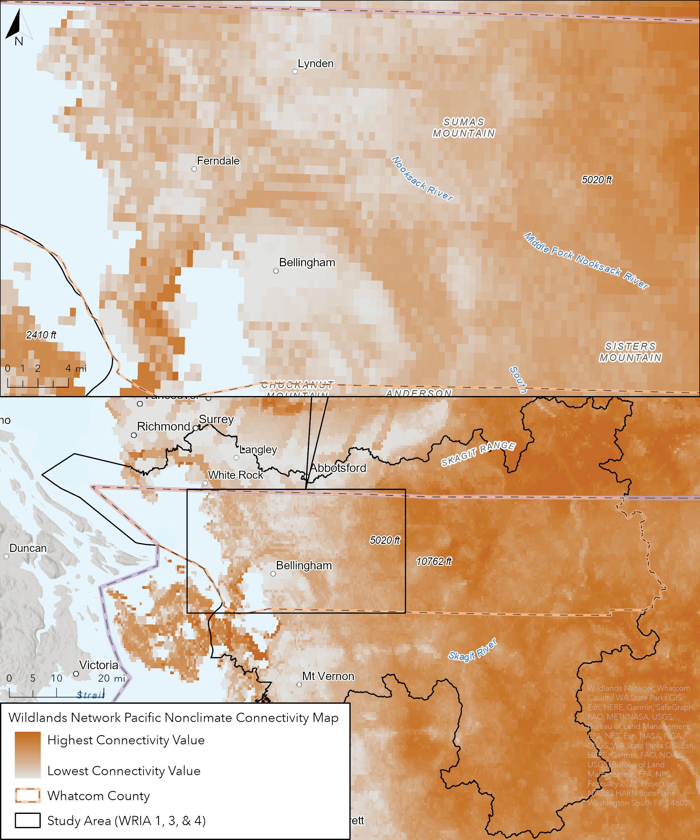Figure B2. Nonclimate connectivity value from Wildlands Network’s Pacific Connectivity Map (Nuñez et al. 2022). This index was used as one of the input datasets for calculating the Wildlife Habitat Connectivity Value index for Whatcom County.

Appendix B: Supplementary Figures

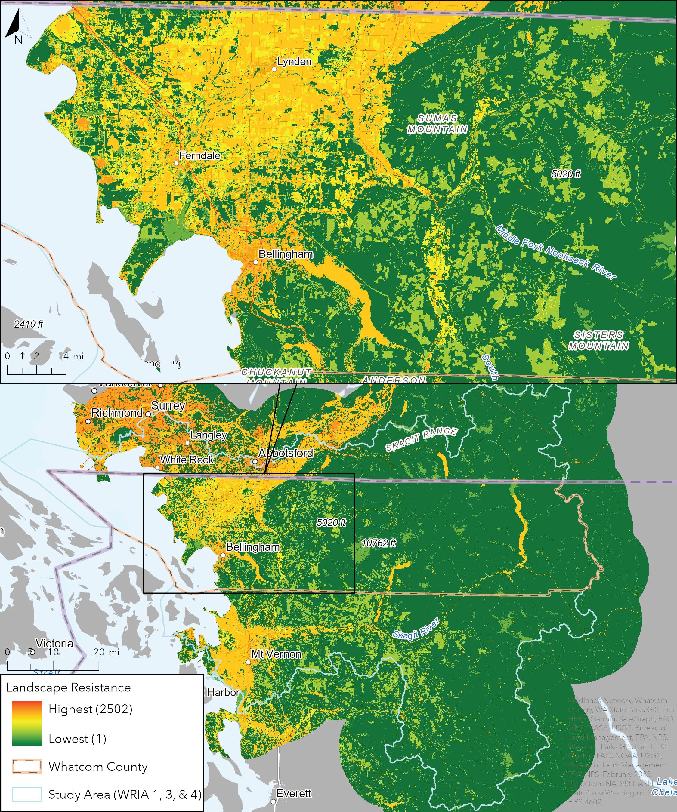Figure B3. Landscape resistance surface for Omniscape representing the relative predicted risk and/or energy cost to generalized, terrestrial wildlife moving across the study area. This is the same as the resistance surface used for Linkage Mapper (Figure 5) except that the resistance from slope has been removed, resulting in lower resistance values especially in the eastern, mountainous part of the study area.

Appendix B: Supplementary Figures

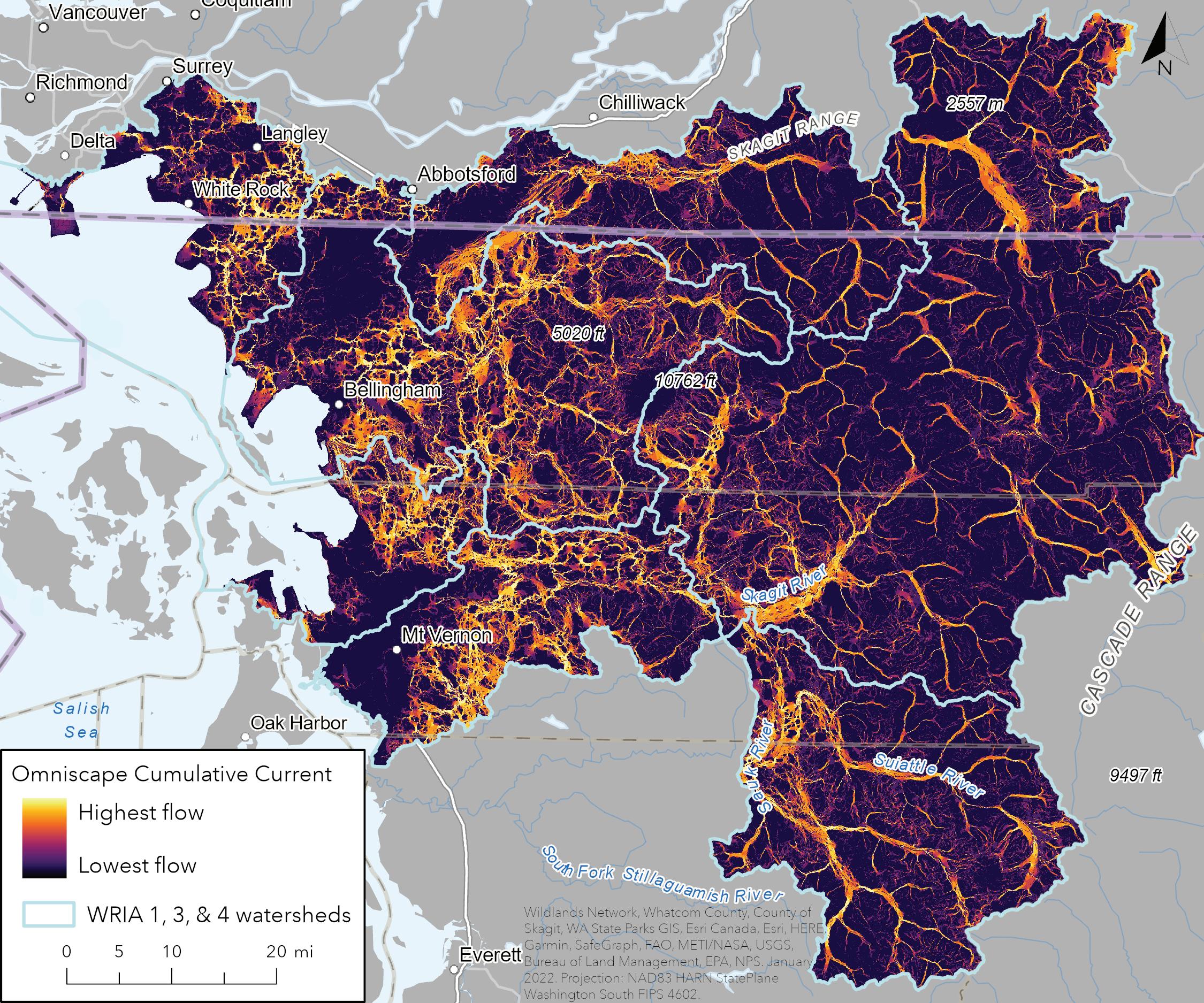Figure B4. Preliminary Omniscape connectivity result calculated using the landscape resistance surface that includes slope resistance (Figure 5). The simulated wildlife current flow was highly channelized all across the study area, even in the mostly natural and broadly permeable east, because of the disproportionate influence of slope in areas that otherwise have very low resistance to wildlife movement. For the final Omniscape result used in this report, we repeated Omniscape using the same resistance surface without slope (Figure B3).