6 minute read
Creating an overall Connectivity Value index


Lastly, we created a summary index of Connectivity Value to show, at a glance, the estimated overall value that each part of the study landscape contributes to wildlife habitat connectivity. This index was a combination of pre-existing connectivity maps and the novel connectivity analyses conducted in this report, described in the sections above, plus a special emphasis on the value of riparian areas for connectivity, as requested by Whatcom County. In total, six different connectivity value scores were calculated and then averaged to calculate Connectivity Value in the WRIA 1, 3, and 4 watershed study area.
Two of these six connectivity scores came from Wildlands Network’s Pacific Connectivity Map. This map, which summarizes dozens of published studies on wildlife habitat connectivity from California to British Columbia, was developed by Wildlands Network and researchers at the
Advertisement
University of Washington (Nuñez et al. 2022). The map includes two connectivity indices: climate connectivity value, based on studies that explicitly address wildlife migration in the face of climate change, and non-climate connectivity value, based on studies that examined present-day connectivity (see maps in Appendix B).
Another three of the connectivity score components came from the landscape resistance layer, Linkage Mapper least cost corridors, and Omniscape results from this report. Landscape resistance was inverted and rescaled so that areas with the lowest resistance had the highest connectivity score. The relative cost-weighted distance from Linkage Mapper’s least cost corridors was also inverted so that the lowest-cost areas were given the highest connectivity score. Cumulative current from Omniscape was rescaled so that the highest current received the highest connectivity score. Finally, the sixth connectivity score simply awarded high value to areas within 100 feet of all streams and waterbodies in the study area (not including the water bodies themselves, which can be barriers to wildlife). This addition was requested by Whatcom County to emphasize the value of riparian
Results
Landscape resistance to wildlife
Using geospatial information about landcover, roads, railways, trails, and slope, we created a landscape resistance layer that represents the predicted risk and/or energy cost to wildlife moving across the study area (Figure 5). Landscape resistance was generally highest in the west near the highly-developed and densely-populated metro areas of Vancouver, Ferndale, Bellingham, and Mt. Vernon. Resistance was moderately high in the agricultural lowlands outside these cities and in the valleys reaching east into the mountains. In the east, largely dominated by the Cascade Mountains where development is limited and roads are few, resistance is generally much lower, and patterns of resistance are governed mostly by steep slopes and wide water bodies that can pose barriers to many terrestrial species.
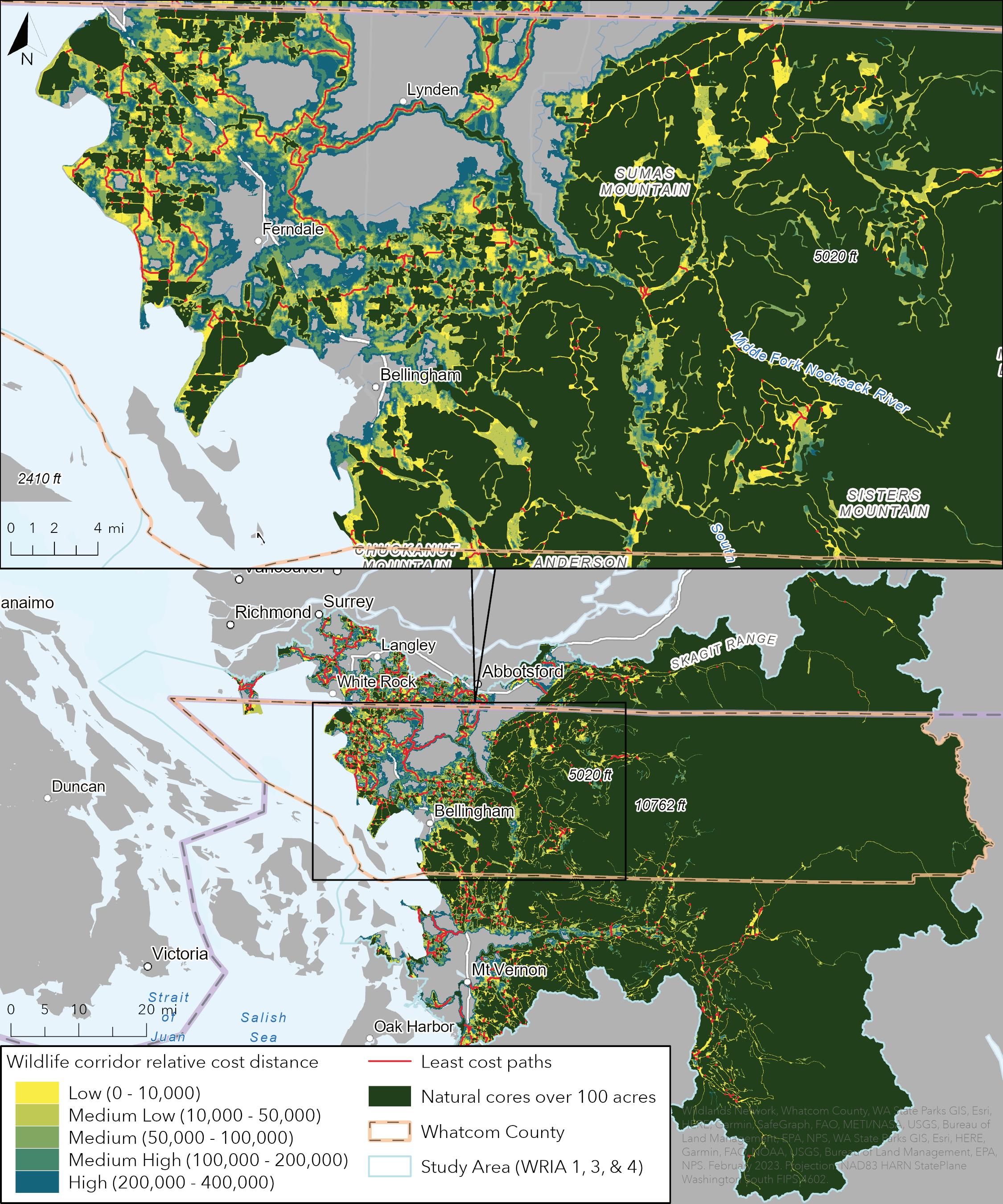
Least cost paths and corridors from Linkage Mapper
We used the landscape resistance layer above along with the habitat core areas we created using the Green Infrastructure approach to conduct wildlife habitat connectivity analyses using Linkage Mapper. The result is a map of 100 acre or larger blocks of contiguous natural landcover connected by a network of least cost paths and least cost corridors (Figure 6). Least cost paths show the optimal path that an animal would take from one habitat core to an adjacent core if it wanted to face the lowest possible amount of landscape resistance. Of course, in reality animals do not have perfect knowledge of the landscape and rarely follow set paths to a corridors for movement of many species and reflect the importance of waterways to planners and managers in the area. certain destination, but least cost paths show us where the cumulative resistance of the landscape between two cores is the highest. Least cost corridors show how costly all other possible paths are relative to the optimal least cost path.
The six scores for (1) Pacific Climate Connectivity, (2) Pacific Non-climate Connectivity, (3) landscape resistance, (4) least-cost corridors, (5) Omniscape cumulative current, and (6) riparian buffers were each rescaled using equal intervals from 0 to 100, where 100 represents the highest connectivity value, and then averaged together to calculate the Connectivity Value index.
All geospatial analyses were conducted using ESRI’s ArcGIS Pro or ArcMap software (ESRI 2022, ESRI 2022).
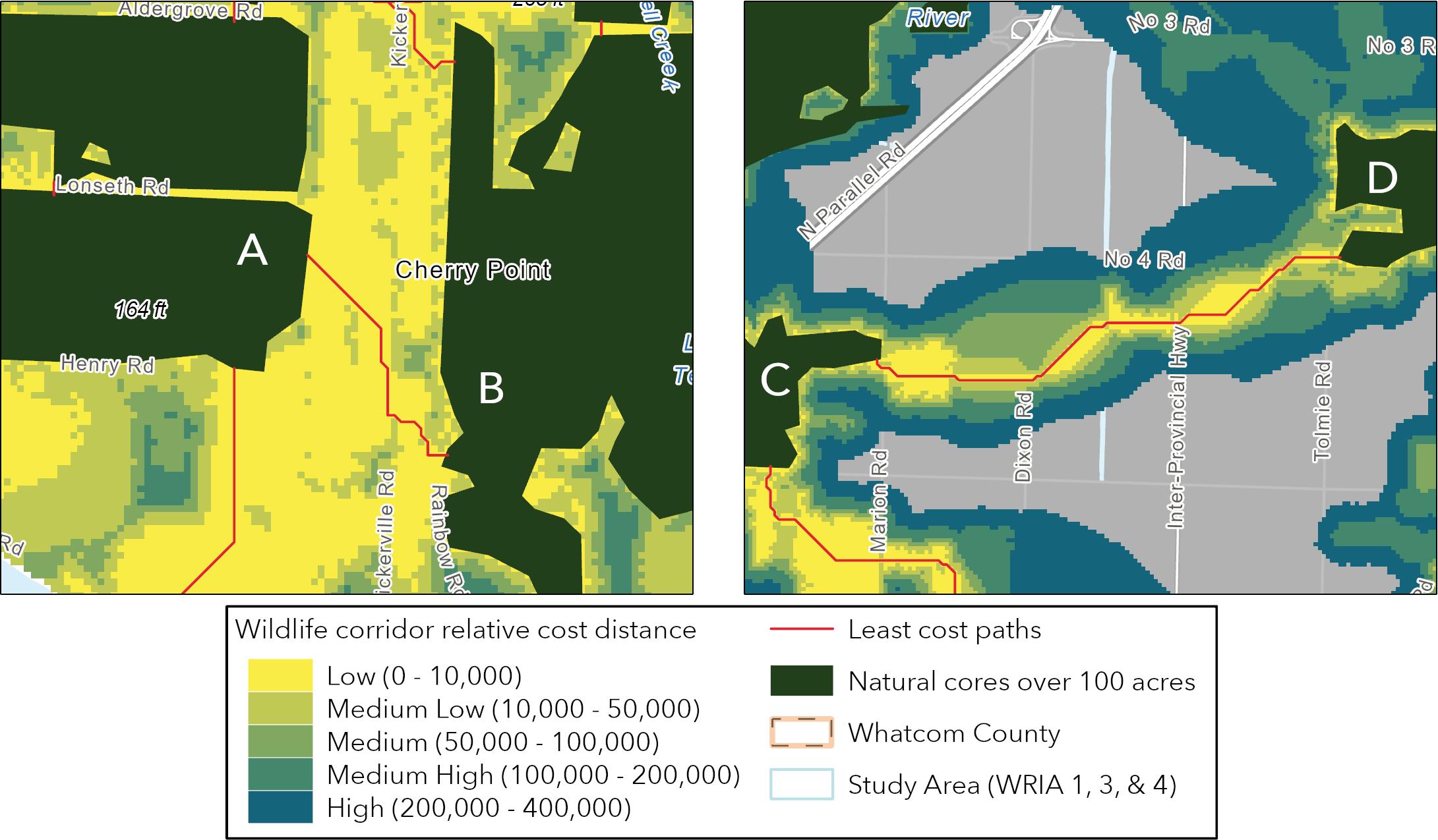
Taken together, least cost paths and corridors can help us understand the nature of connections between adjacent habitat cores. Least cost paths show us the best possible connection, and least cost corridors show how constricted or permeable the connection is. For example, consider these two different connections between core areas (Figure 7): in the first (A to B), the corridor cost is low in a wide area surrounding the least cost path, suggesting that this area is widely permeable to wildlife and that the least cost path is likely not the only practical path; in the second (C to D), the corridor cost rapidly increases around the least cost path, suggesting that this narrow connection is constricted by high landscape resistance on either side. This has direct implications for connectivity management, and in this case suggests that the second connection (B) is a higher-priority target for corridor conservation and/or restoration.
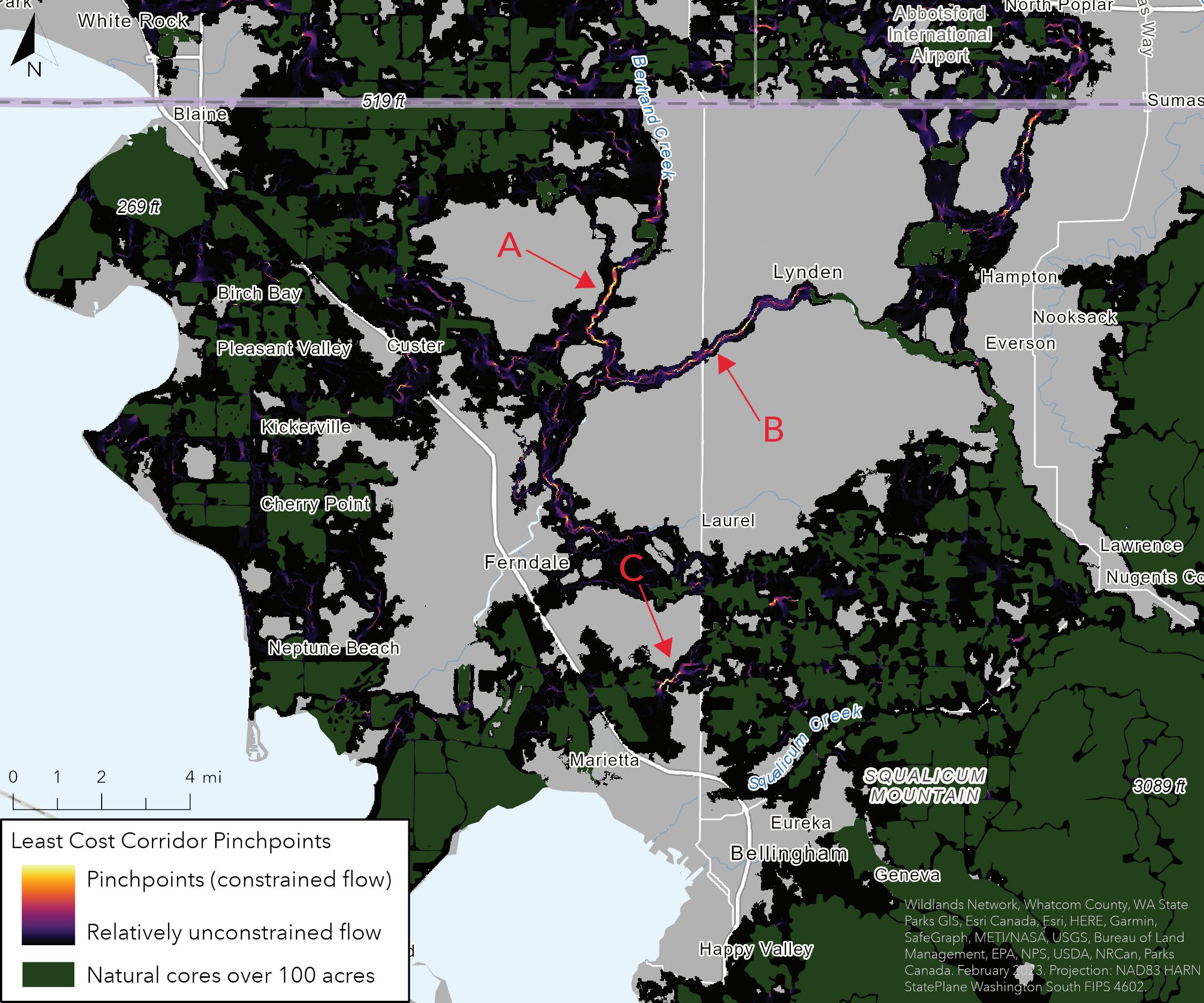
Pinchpoints from Linkage Mapper
After creating least cost corridors, we used Pinchpoint Mapper to find pinchpoints within the corridors where simulated wildlife flow is constrained to narrow bottlenecks. Pinchpoint Mapper is useful for identifying possible high-priority corridors in need of conservation action to prevent further fragmentation from severing vital connections. These pinchpoints could also benefit from restoration that decreases resistance to wildlife flow by improving habitat and/or removing barriers.

Most of the significant pinchpoints occur in the western part of the study area where roads and human populations are denser and least cost paths are often surrounded by high-resistance landscape such as urban development or agricultural fields (Figure 8). For example, two of the most constricted pinchpoints occur along the riparian corridors of the Nooksack River and Bertrand Creek where they are the last remaining natural pathway for wildlife through heavily agricultural lands (Figure 8, A and B). Another notable pinchpoint, squeezed between a Bellingham suburban development and a golf course, is the only modeled connection between Lummi land to the west and the Cascade foothills to the east (Figure 8, C).
Omniscape Connectivity Model
We created an Omniscape model of wildlife habitat connectivity using a version of our landscape resistance layer that did not include slope as a resistance factor. This resistance layer without slope was the input for conductance and its inverse was the input for current source strength. This model simulates wildlife movements of up to 9,990 meters along every possible path across the study area. The resulting map shows cumulative current, which represents the predicted level of wildlife flow (Figure 9). Paths with high values are predicted to be used more often by dispersing wildlife than the surrounding areas. This can be due to a combination of factors including low landscape resistance along the path, high landscape resistance surrounding the path that channelizes flow, and high source strength, which represents the amount of wildlife in the area to use that path.
As expected, the results show a strikingly different pattern of wildlife habitat connectivity in the west and east of the study area. In the west, where landscape resistance is higher due to urban development, agriculture, and roads, simulated wildlife flow is often channelized into tight corridors between the remaining, fragmented natural areas. In the east, where natural landcover dominates, flow is more uniform, indicating that wildlife face fewer movement restrictions and wildlife habitat is more intact and connected.
To understand the results of Omniscape more clearly, we created a map of normalized cumulative current categorized into distinct flow types by dividing cumulative current (predicted wildlife flow across the landscape resistance surface) by flow potential (predicted flow on a null surface with no landscape resistance at all) and dividing the results into four classes. The result is an index that can be used to classify the landscape into categories of flow type: channelized, intensified, diffuse, and impeded (Figure 10). In diffuse areas, wildlife flow is broadly unrestricted and habitat is well-connected with few major barriers. Impeded areas have less flow compared to their surroundings due to barriers and areas of high landscape resistance. Intensified areas show where wildlife flow is higher than the null model because of impedance by adjacent high-resistance areas, and channelized areas have especially high flow where it has been forced into bottlenecks.
Connectivity Value Index
We created a Connectivity Value index as a general, at-a-glance measure of how much each part of the landscape contributes to wildlife habitat connectivity (Figure 11). The inputs to this index came from the Pacific Connectivity Map created by Wildlands Network and the University of Washington; the landscape resistance, least cost path, and Omniscape models created for this report; and a map of riparian areas in the study area. The result is a relative score that can be used to estimate how important a given part of the landscape is for maintaining wildlife habitat connectivity or to identify fragmented areas for restoration.
The Wildlife Habitat Connectivity Value index shows broadly the difference between connectivity in the developed west and the more natural east, as seen in the landscape resistance, Linkage Mapper, and Omniscape results. However, because it is a relative metric, the index can also be used to examine connectivity value in a smaller area like Whatcom County’s jurisdictional boundary and identify the most important lands for wildlife habitat connectivity there. This map also emphasizes the importance of intact riparian corridors to many terrestrial and aquatic species, especially in the western lowlands.