Potential Future Land Loss
of Small Islands of Puerto Rico and the United States Virgin Islands
FINAL REPORT
for
Project Number: R-111-1-10 to University of Puerto Rico
Sea Grant College Program
Mayagüez, Puerto Rico
by David M. Bush
William J. Neal
Pablo Llerandi-Román Chester W. Jackson, Jr.
August 5, 2013
INTRODUCTION
Understanding how shorelines respond to rising sea level is critical for developing sound coastal management and land use planning guidelines, and is even more important when considering the effect on small islands. Commonly applied coastal recession models are less than adequate in predicting coastal evolution. Such models typically lack adequate baseline data or do not consider local complexities in sufficient detail. Add to this the uncertainty of change in rate of future sea-level rise, and most results are not much better than a simple slope/retreat model.
In this study we evaluated potential shoreline change and associated land loss as a result of continuing sea-level rise of selected associated islands of Puerto Rico and the United States Virgin Islands (USVI). Three techniques of predicting change were employed: (1) the simple slope-retreat model, (2) extrapolation of historical shoreline change, and (3) a modification of the Coastal Vulnerability Index (CVI) currently in use in the United States and Canada, but applied here for the first time to small islands. The modification to the CVI required field and remote mapping of the islands to be able to better predict potential changes for each island subenvironment. State-of-the-art software was employed to assess shoreline change and perform CVI analyses for each location using AMBUR and a recently developed hazard-vulnerability assessment tool called AMBUR-HVA.
Outreach was a second major task of the project. To that end, a field- and inquiry-based professional development workshop was held for in-service teachers, graduate students, and informal educators. The original plan was to hold two workshops, one in Puerto Rico and one in the U. S. Virgin Islands. However, owing to financial limitations, a single workshop was held, in Humacao, with attendees from the USVI.
No perfect model exists to predict coastal recession during times of rising sea level. The most commonly used model has been the Bruun Rule (Bruun, 1962). That model and similar
approaches require so many simplifying assumptions as to be rendered useless in real world applications (Pilkey and Davis, 1987; Cooper and Pilkey, 2004). Another approach is to consider geomorphological changes during a shoreline transgression (Carter and Orford, 1993), although this approach must consider a longer time frame than that of interest to the coastal planner and manager.
This study forecasts shoreline change and land loss using three methods. (1) For simplicity, an overview of the setting was established using a coastal slope/retreat model. (2) Next, determination of historical shoreline change using air photo and satellite imagery, and extrapolation of those changes into the future. The former approach presupposes that the dominant control on coastal regression is the offshore/onshore long profile of the area of interest; the latter approach presupposes that “what’s past is prologue.” Good data is available for both approaches and by understanding the limits of the projects, sound results can be obtained. (3) Finally, a more detailed forecast was made by applying a variation of the Coastal Vulnerability Index (CVI, see discussion below). The CVI model looks at shoreline segments based on composition and develops a potential response to sea-level rise for each island subenvironment, and/or unique shoreline stretch.
The mainland coast of Puerto Rico has been and continues to be well studied (Morelock, 1978; Morelock, 1984; Bush, 1991; Thieler and Danforth, 1993, 1994a; Bush et al., 1995; Thieler and Carlo, 1995; Schwab et al., 1996; Bush et al., 2001; Morelock and Barreto, 2003, Donnelly, 2005). The USVI have been evaluated to a lesser degree, for example, Cambers (1997) reported on Eastern Caribbean Island coastal changes. However, much less attention has been paid to the associated small islands. Small islands are important resources for reasons of recreation, cultural, historical significance, and/or development (Maul, 2005). It is clear that the significance of understanding the risks of coastal recession and inundation, plus the sustainability of coastal development, include aspects beyond the evaluation of expected sea-level rise, as noted in studies of Pacific Island Nations (Dickinson, 1999). For these reasons, the study focused on selected small associated islands.
Further, a bilingual workshop for in-service teachers, marine/environmental educators, and graduate students from Puerto Rico, the U.S., and the USVI was developed and presented. The workshop was titled: “Coastal Processes, Geoindicators, and Earth Science Education at the secondary school level.” It was conducted at the Sea Grant facilities of the University of Puerto Rico, Humacao. Participants visited Playa Palmas de Lucía in Yabucoa, the beach south of Punta Tuna in Maunabo, and the rock outcrops in Punta Tuna as part of the workshop. Evaluations of the workshop were obtained from the attendees, and follow-up comments have been obtained.
METHODS
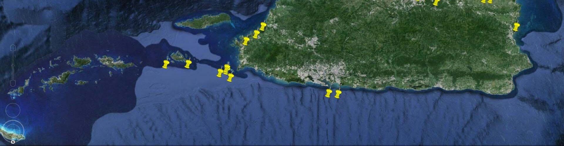
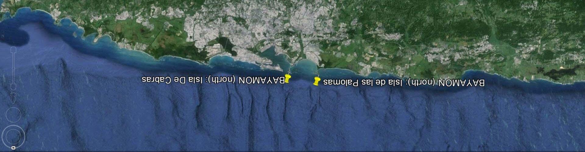
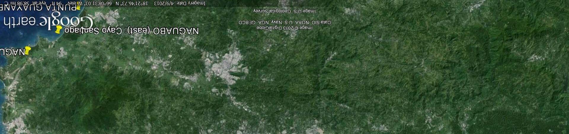
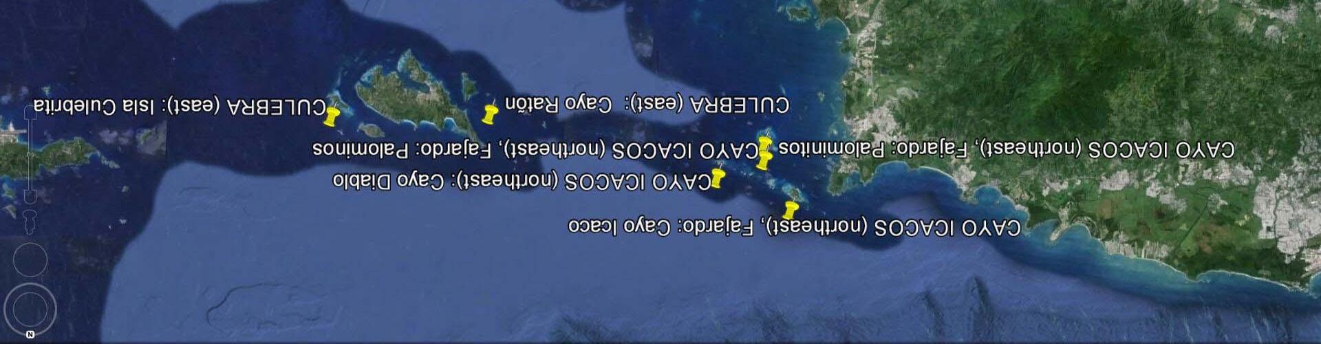
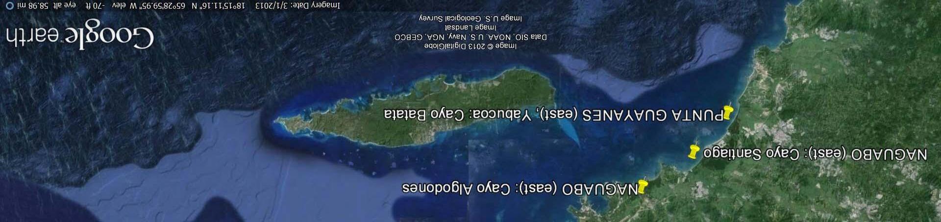
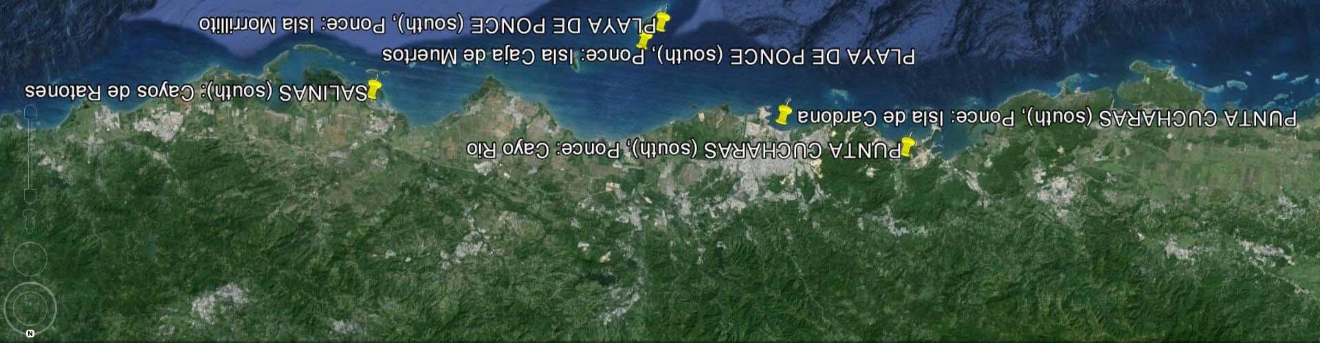
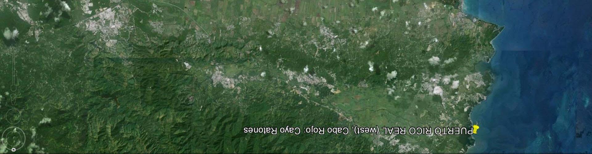
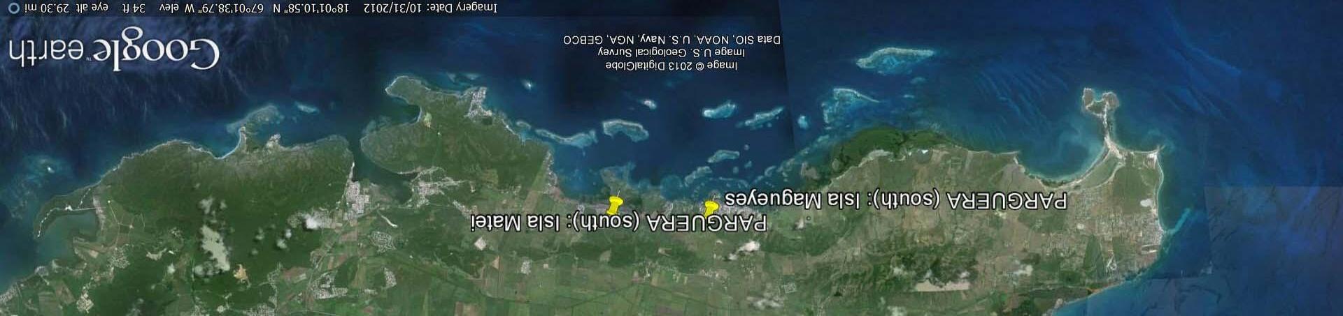
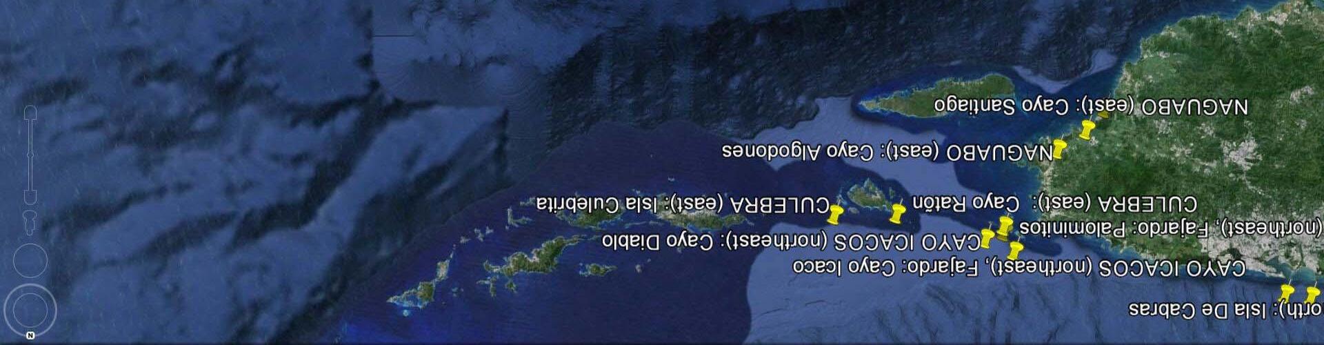
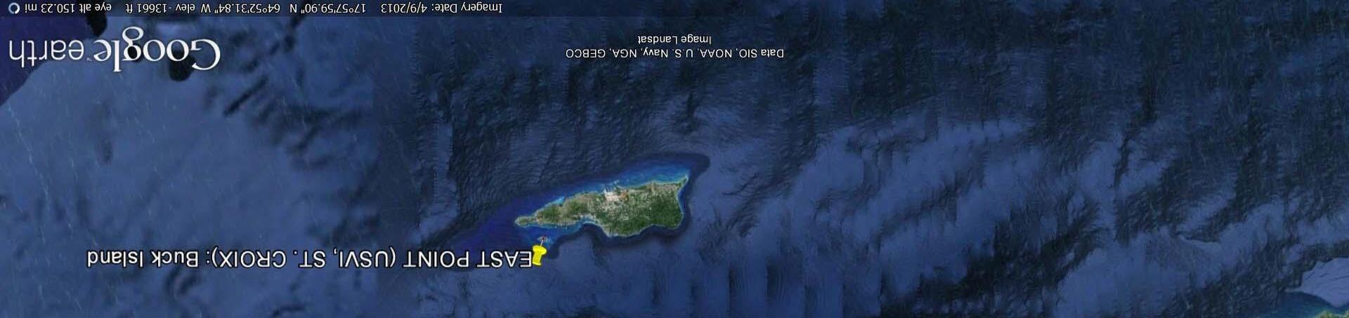
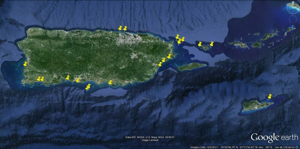
There are well over 100 small islands and cays surrounding Puerto Rico and the U. S. Virgin Islands. Twenty islands were selected for inclusion in the study because they exhibit either historical, cultural, recreational, or scientific importance, or some combination of factors (Table 1, Figure 1, Plates 1-6). Islands that contain benchmarks were considered for inclusion because benchmarks increase the precision and accuracy of the CVI field mapping. Appendix A presents Google Earth images of all the islands in the study. There are several generations of images available within Google Earth. In addition, transects were drawn across the islands in several directions in order to measure island width in various orientations.
The project evolved in three parts, (1) calculating shoreline change, (2) developing and applying a Coastal Vulnerability Index (CVI), and (3) outreach.
Table 1. Islands included in the study.
USGS Quad (location on PR) Island
Bayamón (north)
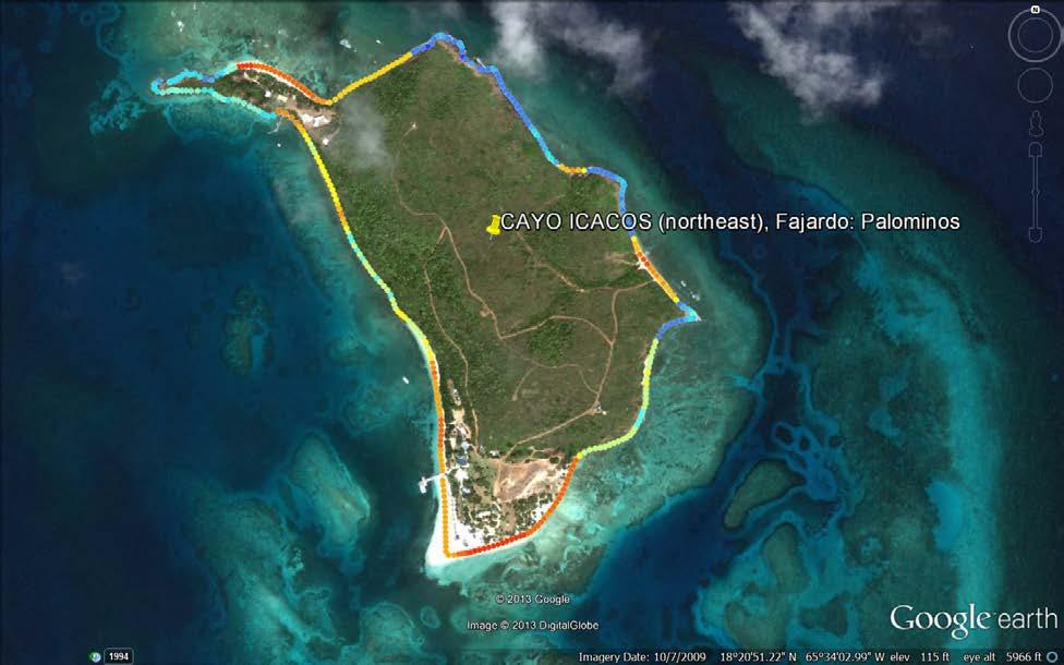
Cayo Icacos (northeast)
Culebra (east)
Naguabo (east)
Punta Guayanés (east)
Salinas (south)
Playa de Ponce (south)
Punta Cucharas (south)
Parguera (south)
Puerto Real (west)
East Point (USVI, St Croix)
Characteristics
Isla de las Palomas Rare northern island
Isla de Cabras Historical and recreational significance
Palominos Reefs, recreation
Palominitos Reefs, recreation
Cayo Icacos Reefs, recreation
Cayo Diablo Reefs, recreation
Cayo Ratón Reefs, recreation
Isla Culebrita
Large, high elevation, and wetlands
Cayo Algodones Sandy, has bench mark
Cayo Santiago Large, forested, has bench mark
Cayo Batata
Very small, has bench mark
Cayos de Ratones Mangroves, lighthouse
Isla Caja de Muertos
Isla Morrillito
Isla de Cardona
Cayo Río
Isla Magueyes
Isla Matei
Cayo Ratones
Large, lighthouse, recreation
Sandy, associated with Caja de Muertos
Small, lighthouse, reefs
Medium size, near port, reef
UPR Marine Station, mangroves
Large, high elevation, mangroves
Small, erosion problem
Buck Island National Park
Shoreline Change Methods
Shoreline change was approached in two ways. First, what would happen to an island shoreline assuming rapid (essentially instantaneous) sea-level rise on an unchanging land surface (the slope/retreat model). This is sometimes also referred to as “filling the bath tub” and seeing how the shoreline changes. It is largely dependent on the slope of the island itself. Second, measuring the historical evidence from air photos and satellite imagery, shoreline position change is analyzed. Along with digitizing the position of historical shorelines, the most recent shoreline was classified and digitized by shoreline type. This provided a catalog of shoreline segments to later be applied to a vulnerability analysis.
Slope/Retreat Calculation
Shoreline recession based on migration surface slope gives an idea of shoreline retreat based strictly on the slope of the island surface to be transgressed given a specific rise in sea level. Sea-level rise and resultant transgression are assumed to occur instantaneously under this scenario, so that slope of the flooded surface would be the only control on shoreline recession. NOAA has an on-line sea-level rise viewer with data from Puerto Rico, the Sea Level Rise and Coastal Flooding Impacts Viewer (NOAA, 2011) As such, we decided to forgo calculating and plotting slope-retreat maps in deference to the already-available NOAA tool. The NOAA Sea Level Rise and Coastal Flooding Impacts viewer may be accessed at http://www.csc.noaa.gov/slr/viewer/#. It should be noted that NOAA has attempted to calibrate the elevations of their 3D models from geodetic datum (PRVD02) to a tidal datum of mean higher high water (MHHW) for better modeling with aerial LiDAR data. However, it was determined that future work is needed to better calibrate aerial LiDAR to tidal datums given vertical errors (1+ meters) that exist with PRVD02 datums. Terrestrial LiDAR was used to produce a high resolution elevation model of Cayo Ratones and calibrated to the instantaneous
mean high water line observed. This provided centimeter vertical accuracy and a better 3D surface model of the cay and holds great promise for future studies of cays in Puerto Rico.
Historical Shoreline Change
Historical shoreline change was calculated using AMBUR software (Jackson et al., 2012) and employed the methodology that was defined in the in the manuscript by Jackson et al., (2012). Monitoring changes in the position of the shoreline or other shoreline markers indicates the dynamics between sea-level change, sediment supply, hydrography, and meteorology. The actual shoreline, dividing line between land and the marine realm, is the most obvious line of demarcation. Perhaps no information is more critical for coastal management than shoreline change history.
Historical shoreline change is typically determined using aerial photographs from as many different surveys as possible preferably with at least one set of photos from each decade. Thieler and Danforth (1994b) used air photo data for the main island of Puerto Rico up through the 1980s. For this study, shorelines from NOS T-sheets and LiDAR data were used along with air photos.
The more generations of air photos covering the larger amount of time, the better the data will be with fewer errors. Methodology and discussions on shoreline position errors are presented in several studies (e.g., Crowell et al., 1991; Douglas and Crowell, 2000; Moore, 2000; and Thieler and Danforth, 1994a & b). All shoreline positions have some degree of inaccuracy, and such errors should be reported so that rate-of-change calculations may be interpreted and used judiciously. Newly developed digital shoreline analysis systems (Jackson et al., 2012) can take a shoreline position and forecast a new shoreline position using a sea level rise rate and a beach slope It can also forecast using traditional rate methods and can be modified to incorporate other parameters (Jackson et al., 2012).
Historical shoreline position data was digitized from NOAA t-sheets and aerial photographs (Table 2). Accuracy of shoreline position obtained from the air photos is much better than that from the t-sheets. The historical shorelines were digitized as continuous lines.
The Shoreline position rate of change calculated using end point rate in the AMBUR program (Jackson et al., 2012) as discussed previously. AMBUR was set to derive transects every 10 meters, resulting in a total of 5,234 transects among all the study area islands. The length of all shorelines digitized totaled 106km. The total area of all the islands in the study was 609.97 hectares, just over 6 square kilometers.
Table 2. Inventory of data used for shoreline change analysis.
Coastal Vulnerability Index Methods
A Coastal Vulnerability Index (CVI) incorporates geologic and physical process variables that are dominant in the coastal system, and provides a relative yet quantitative measure of vulnerability. The CVI accounts for the dynamic nature of the coast and reflects its sensitivity to change with respect to rising sea level.
Small islands of the Northeastern Caribbean are discrete environments that lack study in any great detail. It was therefore necessary to utilize a variable set appropriate to the environmental conditions of the study area. The lure of the CVI approach lay in its flexibility to
be modified based on the question, the geologic setting, and the oceanographic regime of interest. Many coastal vulnerability assessments using the CVI technique occur in the literature, each of them using a format designed to suit the study area. The CVI was originally developed by Gornitz and Kanciruk (1989) for the mid-Atlantic region; see also Shaw et al. (1998), Thieler and Hammar-Klose, (1999) and Wood (2009) for a review of formats.
There are several reasons for examining small islands exclusively in this regard. First, many small islands in the Northeastern Caribbean are recognized for scientific, historical, and/or cultural/recreational significance. Islands of this size are convenient grounds for the testing of new models, because they are mostly removed from the influence of anthropogenic activity and development (Nunn, 1986). For the main islands of Puerto Rico and USVI, this phenomenon is emphasized due to extensive development in the coastal zone. Therefore, small associated islands can be considered more naturally intact environments than those subjected to anthropogenic disturbance. In some ways, small islands approximate the compartmentalized beach systems of the main island coast; both environments are characterized by little to no communication of energy between adjacent systems. Furthermore, processes shaping the main island coast will incur change more rapidly over the smaller surface area of a small island. This capacity for sensitivity to change over a shorter period of time suggests small islands as a potential proxy for future shoreline change.
In an effort to optimize coastal resource management for U.S. National Parks, the USGS and National Park Service (NPS) employed a CVI in their National Assessment of Coastal Vulnerability to Sea Level Rise (Thieler and Hammar-Klose, 1999). In this series of CVI studies, the variable set included: Geomorphology, Historical Shoreline Change Rate (m/yr), Regional Coastal Slope (%), Relative sea-level change (mm/yr), Mean significant wave height (m), and Mean tidal range (m). Most of the shorelines analyzed were large and continuous, with the exception of St. John’s Island of the USVI and Dry Tortugas National Park in Florida.
Owing to its setting in the Northeastern Caribbean, the vulnerability assessment for St. John’s was used as a comparative basis for our modified CVI assessment. Modification of the variable set to reflect coastal vulnerability to sea level rise for PR/USVI was required due to differences in the geologic, oceanographic, and climatic settings of the Northeast Caribbean and the continental United States.
Most of the selected islands have not been previously studied, are not easily accessible, or are far removed from tidal gauges. Thus, much of the data are approximate and therefore quite preliminary. To address these issues, detailed field mapping was completed for several islands including Cayo Ratones, Isla de Cardona, and Isla Magueyes
The powerful advantage of this approach is that the proposed CVI may be refined and applied for similar vulnerability assessments of the main islands of Puerto Rico and the U.S. Virgin Islands. A refined and complete CVI for this region would improve the factual basis for coastal management in the Northeastern Caribbean. Accurate vulnerability assessment in this area also has large economic and scientific implications. The risks associated with sea-level rise in the Northeastern Caribbean greatly affects its residents, as current population densities are highest in low lying areas. Additionally, these areas rely on tourism as a major revenue source. Revenue from tourism is diminished by eroding shorelines and failing structures. Mitigation is possible after an erosion problem has developed, but the cost to maintain these efforts becomes tremendous over time. Soft stabilization (i.e., beach nourishment) and hard stabilization (seawalls, groins, etc) both require regular monitoring and maintenance. Therefore, preventative action and understanding the potential for erosion and inundation is much more effective and cost efficient. As populations increase, more people will be forced into coastal areas. In light of
projected sea level rise scenarios, which may rise as much as 10 to 23 inches by the year 2100 (IPCC AR4, 2007), it is evident that the need for effective, accurate and preventative coastal zone management is dire.
CVI Parameters
Applying a Coastal Vulnerability Index (CVI) starts with assessing which geomorphic and physical parameters are most important in driving coastal processes in the study area. Once the parameters are determined and weighted, the CVI can be applied to each shoreline segment. Sea-level rise is incorporated into the CVI. Predicting change is critical for proper coastal zone management and land use planning. However, the lack of complete understanding of the variables and processes of coastal forcing and the disagreement among researchers on which quantitative approaches are valid severely restricts satisfactory outcomes of such studies (Gutierrez et al., 2007).
Because of such complexities and disagreements, an approach was developed for predicting future shoreline regression and land loss called the Coastal Vulnerability Index. The approach is based on evaluations of geomorphic and physical parameters of the coastal system in question that have major influence over the natural vulnerability to the effects of sea-level rise (Gutierrez et al., 2007). The method has been widely applied (see Gutierrez et al., 2007, for a summary). Of special relevance to this proposal are several U. S. Geological Survey Open-File reports dealing with small National Park islands similar in many regards to those considered for study in Puerto Rico and the USVI. For example, Virgin Islands National Park (Pendleton et al., 2004a), Dry Tortugas National Park in Florida (Pendleton et al., 2004b), and the National Park of American Samoa (Pendleton et al., 2005). In addition, the coast of Canada is evaluated by (Shaw et al., 1998). Although at a much larger scale, the Canadian study includes many small islands and a variety of geologic shoreline types, thus sharing some similarity with the small islands of the proposed study.
As originally developed by Gornitz and Kanciruk (1989), Gornitz (1990, 1991) and Gornitz et al. (1991), the Coastal Vulnerability Index utilized six variables. Shaw et al. (1998) modified the approach for application in Canada to include seven variables. The U. S. Geological Survey approach is the most widely published version and utilized six variables. It was based on an earlier database developed by Gornitz and White (1992). For comparison, the six variables utilized by the USGS (from Thieler and Hammar-Klose, 1999) versus the seven variables used by Shaw et al. (1998) are given below for illustration purposes.
The six variables utilized by the USGS (from Thieler and Hammar-Klose, 1999) are: -geomorphology, -shoreline erosion and accretion rates (m/yr), -coastal slope (percent), -rate of relative sea-level rise (mm/yr), -mean tidal range (m), and -mean wave height (m).
The seven variables used by Shaw et al. (1998) in Canada are: -relief -rock type
-coastal landform
-sea-level tendency
-shoreline displacement rate
-mean tidal range (higher tides)
-mean annual maximum significant wave height
Rankings of each variable within the Coastal Vulnerability Index utilized by Thieler and Hammar-Klose (1999) are given in the Table 3. Obviously some of the variables above are not applicable to small islands. For example, for a single small island, mean tide range will likely not vary, not have been measured, or will not easily be measured. The same holds for mean wave height. This meant that we had to assess which parameters are most pertinent to Puerto Rico and USVI and would need to be ascertained and incorporated.
Table 3. CVI paramers used by Thieler and Hammar-Klose (1999).
Ranking of Coastal Vulnerability Index (from Thieler and Hammar-Klose, 1999) Very low Low Moderate High Very high VARIABLE 1 2 3
Geomorphology
Rocky, cliffed coasts Fiords Fiards
Medium cliffs Indented coasts Low cliffs Glacial drift Alluvial plains
Cobble beaches Estuary Lagoon Barrier beachs Sand Beaches Salt marsh Mud flats Delta Mangrove Coral reefs
Our revised CVI utilized only four parameters: -shoreline composition -sea level change -slope -shoreline change rates
Shoreline composition
Shoreline composition was determined from field work, air photos, satellite imagery, and an Environmental Sensitivity Index (ESI) produced by Research Planning Institute, Inc. (RPI) (Zengel et al., 2001). The ESI was developed for oil-spill contingency planning and response and
coastal resource management. As part of the ESI assessment, the shoreline is classified into ten categories some with subcategories for a total of 15 coastal classification categories. The ESI categories are presented in order of increasing sensitivity to spilled oil. The data are available digitally and were incorporated into our evaluations. The 15 classes were collapsed into five weighted categories for use within our CVI. The shoreline classifications in our CVI are, of course, in order of increasing vulnerability to coastal change.
Coastal shoreline habitat classification (Zengel et al., 2001), in order of increasing sensitivity to spilled oil:
la. Exposed rocky cliffs
lb. Exposed, solid man-made structures
2a. Exposed wave-cut platforms in bedrock
2b. Scarps and steep slopes in muddy sediments
3. Fine- to medium-grained sand beaches
4. Coarse-grained sand beaches
5. Mixed sand and gravel beaches
6a. Gravel beaches
6b. Riprap
7. Exposed tidal flats
8a. Sheltered rocky shores
8b. Sheltered, solid man-made structures
9a. Sheltered tidal flats
9b. Sheltered, vegetated low banks
10. Mangroves
Shoreline classification categories in our modified CVI, in order of increasing vulnerability to coastal change, that is, increasing erodibility or mobility of the substrate:
1. Rocky shores and platforms; seawalls
2. Gravel beaches and riprap; Sheltered mangroves
3. Mixed sand & gravel beaches and fill; Exposed mangroves
4. Coarse-grained sand beaches; Sheltered tidal flats
5. Fine-grained sand beaches; Exposed tidal flats
Particular importance was placed on shorelines dominated by mangroves, which can offer protection to land areas behind them by dampening wave energy. Wave height, and thus flux of energy, can be reduced as much as 66% through 100 meters of mangroves as mangrove roots and lower branches act as physical barriers (McIvor et al., 2012a).
Mangroves have also been shown to reduce the effects of storm surge (Krauss et al., 2009; Zhang et al., 2012) and from erosion (Thampanya et al., 2006). Mangroves slow water movement and block wave energy. Storm surge may be reduced as much as 50 cm per kilometer of mangrove width and waves by at least 75% over that distance (McIvor et al., 2012b). Of course, on the small islands in this study there are no sites with 1 km of mangrove, however, some attenuation of energy is expected, and the model will hold for islands outside the study area.
Some indication of the reduction of flow velocity over various types of ground surfaces is giving by the Manning coefficient of friction (also called simply the Manning number and denoted by the symbol n) (Li and Zhang, 2001). When water flows over a land surface, regardless of whether or not it is confined in channels, is driven purely by gravity such as in rivers or overland flow, or is pushed by storm surge, the friction between the flowing water and the land creates a drag force
which causes expenditure of energy and thus can dampen water flow velocity. Any vegetation present can increase the roughness of the boundary surface and further reduce flow velocity (Chow et al. 1988; Jin et al., 2000).
Some examples of experimentally derived Manning numbers are given in Chow (1959) and Mattocks and Forbes (2008):
Open water/sand
Scattered brush/shrub/scrub
Forest/estuarine forested wetland
Dense woods
0.02
0.05 (0.035 to 0.07)
0.10 (0.08 to 0.12)
0.15 (0.11 to 0.20)
For illustration purposes, a Manning coefficient of 0.02 will theoretically allow a flow velocity five times the speed of a land surface with a coefficient of 0.1. Thus water flowing over a sandy surface could flow five times faster than water flowing over forested wetland. Mazda et al. (1997) report Manning coefficients as high as 0.4-0.7 in some mangrove swamps. Acrement and Schneider (1989) review coefficients for flood plains.
Not only do they block wind, wave, and storm surge, another aspect to the importance of mangroves is their sediment-trapping capabilities, which allow wetland surfaces to keep pace with sea level rise (McIvor et al., 2013). Though Cahoon et al. (2006) reports sediment surfaces lagging behind sea-level rise. Studies in Twin Cays, Belize, report mangrove surfaces being maintained for thousands of years (McKee et al., 2007; McKee, 2011). These studies stress the importance of protecting mangroves and maintaining an unimpeded surface over which they can migrate as sea level rises.
Sea-Level Change
In addition to being useful for coastal planning and management in the short term (up to 10 years, for example), projections of shoreline position 50 and 100 years into the future are useful for long-term planning. An analysis of sea-level change data is reported by the Puerto Rico Climate Change Council (PRCCC) (2013). The current rate of sea-level rise will result in a rise of 0.4 meters by 2100 (Figure 2). According to the report, if the observed Puerto Rico sea level rise trend continues linearly, with no acceleration in rate, by 2100 the sea level around Puerto Rico will have risen by at least 0.4 meters. The U.S. Army Corps of Engineers (USACE) conducted an analysis for the PRCCC to project possible future sea level rise for the North and South coasts to 2165. Sea-level rise estimates range from 0.07 to 0.57 meters (0.20 to 1.87 feet) above current mean sea level by the year 2060 and between 0.14 and 1.70 meters (0.40 to 5.59 feet) above current mean sea level by the year 2110. In order to produce maps of projected shoreline position, the low, moderate, and high rates of sea-level rise were utilized (Table 4). Results are shown in the Addendum to follow this report.
Table 4. Projected sea-level positions assuming a low, moderate, and high rate of sea-level rise over the next 50 and 100 years. Numbers are relative to current sea level. Data from PRCCC (2013).
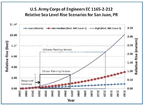
Figure 2. Sea level rise projection scenarios for Puerto Rico through 2150 (Puerto Rico Climate Change Council (PRCCC) 2013).
The current rate of sea-level change was obtained from NOAA tide gauge station information. San Juan and Isla Magueyes have the two longest operating gauges in Puerto Rico. Charlotte Amalie, St. Thomas, USVI, also has a long-operating station. We decided it was most expedient and accurate to use only the data from these three stations. The value for the San Juan station is 1.65 +/- 0.52 mm/yr over the time period of 1962 to 2006, equal to to a change of 0.54 feet in 100 years (NOAA Sea Level Trends web page: http://tidesandcurrents.noaa.gov/sltrends/sltrends_station.shtml?stnid=9755371). For Isla Magueyes, the trend is 1.35 +/- 0.37 mm/yr over the time period 1955 to 2006 which is equivalent to a change of 0.44 feet in 100 years (NOAA Sea Level Trends web page: http://tidesandcurrents.noaa.gov/sltrends/sltrends_station.shtml?stnid=9759110). For Charlotte Amalie mean sea level trend for Charlotte Amalie, St. Thomas, USVI, is 1.20 millimeters/year with a 95% confidence interval of +/- 0.96 mm/yr based on monthly mean sea level data from 1975 to 2006 which is equivalent to a change of 0.39 feet in 100 years. From NOAA Sea
Level Trends web page http://tidesandcurrents.noaa.gov/sltrends/sltrends_station.shtml?stnid=9751639.
In the rates from the three stations are so similar as to be essentially the same. In fact, on the CVI (see below) all three fall into the same weighted category. It should also be noted that modern GPS constraints are providing estimates for the magnitude and direction of tectonic plate movement of the Puerto Rico–Virgin Islands platform (Grindlay et al, 2005; Mann, 2005). Ideally, future CVI assessments for this area should incorporate measures of neotectonic subsidence/uplift to corroborate against the calculated rate of relative sea level rise. Unpublished preliminary subsidence data for Puerto Rico seems to indicate that Puerto Rico is undergoing subsidence faster on the northeastern/north coast which may have a greater impact than global sea-level rise.
Shoreline Change
Given that there has yet to be an accepted method adopted by both industry and academia for analyzing shoreline change, AMBUR was employed to calculate changes and produce a variety of statistical data (Jackson et al., 2012). The advantage of using AMBUR is that it provides a tool for assessing highly curved/sinuous shorelines that are difficult to assess using existing tools. Furthermore, transects and data generated with AMBUR can be used with the newly developed AMBUR-HVA tool to calculate a CVI for different shoreline types and localities. The program calculates shoreline change by measuring the position differences of two or more historical shorelines along transects. Transects were cast at orientations approximately normal to, or in the direction of shoreline movement along a baseline at a spacing interval of 10 m for this study. Each transect captured the shoreline change distances and rates between the oldest and modern shoreline.
Slope Data
Slope data was primarily derived from USACOE 2004 aerial LiDAR that was provided by NOAA’s Coastal Services Center. Bare-earth LiDAR points were used to produce a 3D surface or grid that was approximately 1-meter per pixel. The algorithm used to construct digitial elevation models (DEM) for each location was ANUDEM, a robust 3D modeling/surfacing program. The percent slope was calculated in ArcGIS 10.1 for each pixel the in DEM. Transects were cast alongshore at 10 meter spacing and at least 20 meters inland and offshore of the historical shorelines and intersected with DEMs of each location. The mean slope was calculated for each transect using AMBUR-HVA.
Coastal Vulnerability Index Calculation
The final weighting of CVI parameters is given in Table 5. Geomorphology was mapped but not used in the analysis. The idea behind geomorphology was that it is a representation of island composition and land cover. That is, what is the shoreline going to encounter inland from the current shoreline as sea level rises. There seemed to be a lot of redundancy between
shoreline type and our developing geomorphology category that we decided to abandon geomorphology as a CVI input, though it is retained in Table 5 for illustration purposes.
Table 5. Final CVI parameter weighting.
Geomorphology
Shoreline type (ESI Categories)
(after Zengel et al., 2001)
Resistant rock (igneous, metamorphic, siliciclastic)
Rocky shores and platforms; seawalls (1)
Non-resistant rock (limestone, eolianite)
Gravel beaches and riprap; Sheltered mangroves (6,8)
Unconsolidated sediment, gravel
Mixed sand & gravel beaches and fill; Exposed mangroves (5,2)
Unconsolidated sediment, vegetated
Coarse-grained sand beaches; Sheltered tidal flats (9,4)
Unconsolidated sediment, unvegetated
Fine-grained sand beaches; Exposed tidal flats (7,3,10)
The Coastal Vulnerability Index calculation is very simple (Equation 1). The index parameters are weighted on a 1-5 scale. For each parameter, 1 denotes a very low probability of coastal change, 5 being the highest probability of coastal change. The beauty of a CVI is that it can incorporate a wide range of types of input parameters, but as long as they are weighted, their relative importance is shown. Within AMBUR, CVI is calculated as the square root of the product of the ranked variables divided by the total number of variables Thieler, E. R and Hammar-Klose, E. S. (1999).
Equation 1. Final applied CVI calculation:


Outreach: Geoscience Education Activities
A geoscience education, field- and inquiry-based workshop designed to enhance the understanding of concepts related to coastal geomorphology and dynamics took place at the UPR-Sea Grant facilities at Humacao in July 20-22, 2011. In-service teachers, graduate students, and informal educators from Puerto Rico and the USVI participated in the workshop.
The workshop presented a great opportunity to expose participants to the interdisciplinary and systemic approach to coastal research. This approach aligns naturally with recent national and international recommendations stressing the importance of developing systemic skills, integrating knowledge, and promoting inquiry in geoscience education to improve conceptual knowledge (UCAR-TERC, 2007; TERC, 2007; King, 2001). In addition to enhancing conceptual knowledge through systemic thinking and inquiry, Llerandi-Román (2007) showed that positioning the geoenvironmental context of learning at the core of teaching and learning objectives was also effective in developing inservice teachers’ social responsibility and students’ cultural and ecological identities or worldviews. For these reasons, the outreach activities were designed in order to develop meaningful learning experiences related to coastal processes and coastal geomorphology, including the use of geoindicators in assessing coastal conditions in their local and neighboring coastal communities. The project investigators have remained (and will remain) accessible to assist in the future implementation of coastal science/science education activities in the classroom and the field.
The geoscience education workshop followed a contextual/meaningful learning conceptual model for curricular development in which relevant questions related to shoreline response to relative sea level changes and other coastal processes constituted the core of the curriculum similar to the model implemented in Llerandi-Román (2007, p. 51-55). Specific content was selected based on a needs assessment questionnaire distributed to participants before the workshop, and a content analysis of the Puerto Rico Department of Education (PRDE) Science Curricular Framework, PRDE Content Standards and Grade Level Expectations, and the National Science Education Standards (DEPR, 2007; INDEC, 2003; NRC, 1996). Activities focused on developing understanding of: (a) current geoenvironmental conditions affecting the local coastal region in Puerto Rico and the USVI; (b) content/conceptual knowledge of coastal processes and coastal geomorphology; and (c) transforming content/conceptual knowledge into effective teaching strategies in the classroom. The latter refers to the concept of Pedagogical Content Knowledge (PCK) (Shulman, 1986) or the knowledge to teach science content/concepts in specific contexts as a result of teachers’ solid understanding of pedagogical approaches, student learning skills, and science (Appleton, 2008).
Two workshops had been proposed, one in Puerto Rico and one in the U. S. Virgin Islands. However, owing to resource constraints, we decided on one workshop (in Humacao) and inviting and funding participants from the USVI. It is important to acknowledge Lesbia Montero (Sea Grant Program at UPR-Humacao) and Christine Settar (Sea Grant Program at U. of Virgin Islands), who were of great help in organizing the workshop and in contacting teachers (workshop participants) from Puerto Rico and the US Virgin Islands. Dr. Llerandi-Román was the leader of the survey development and he and Dr. Jackson developed and taught the workshop.
A main goal of the outreach portion of the project was to develop and disseminate a Nive l de l ma r y geoindicadore s (Sea - leve l chang e and geoindicators) survey for workshop participants. T his survey was developed using the SurveyMonkey® online platform and services and after going through extensive revision and face validity assessment by
Llerandi-Román and Jackon. The survey questions included both open-ended and Likert-type items in the online platform. SurveyMonkey® generated a secure link that was sent through email by Lesbia Montero (Sea Grant Program at UPR-Humacao) to all workshop participants. Workshop participants answered the online survey before the first day of the workshop.
The online survey was active for several months before and after the workshop. The registration and monthly fee for services in SurveyMonkey® was covered by a professional development allocation for Llerandi-Román by the Department of Geology, GVSU. The survey was completed by 16 Puerto Rican and U.S. Virgin Islands teachers participating in the coastal resources workshop. Results show that 57% of the participants have never taught sea level concepts in the past. The participants’ level of understanding of sea level change and the causes of sea level change is inadequate and contains misconceptions, for example: [related to understanding of the concept] “Sea level change is the change in the amount of water in the ocean, resulting in a different tidal range” and [related to causes] “Changes in Earth's composition - such as glacial melting, drought, major earthquakes”. Another interesting result from the survey, that can assist teacher educators in the future, is that teachers’ sources of information about sea level change derive mainly from Internet news and science websites (82% of participants) and radio and TV news (57%); only 44% of participants reported learning through professional development. Detailed information about participant responses is found in the summary survey report in the Appendix E.
The final format for the workshop was developed over several months and the final revision was based on the participant responses to the online survey. The workshop ran during the period of July 20-22. The final title of the workshop was “Procesos costeros, geoindicadores y la enseñanza de ciencias terrestres a nivel secundario [Coastal processes, geoindicators, and earth science education in secondary school] – A bilingual (Spanish-English) field-based workshop, UPR Sea Grant Program, UPR, Humacao.” Participants (see workshop Appendix F): 20 Puerto Rico and US Virgin Island in-service teachers, marine educators, and University of Puerto Rico, University of Virgin Islands, and University of Toledo, Ohio graduate students.
RESULTS AND FINDINGS
The project generated a tremendous amount of data and output maps, presented in the appendices. We present here summary findings of each aspect of the project. The most important findings of the project are the results of the shoreline change analysis, the coastal vulnerability analysis, and the workshop impact.
Historical Shoreline Change Analysis
Summary shoreline change statistics of all the islands are given in Table 6. Individual transect locations are plotted using Google Earth. Figure 3 is a Google Earth plot of shoreline transect locations around Cayo Palominos. Red and blue dots are locations of transects Red dots indicate transects with net erosion and blue dots indicate transects with net accretion. Shoreline type is not considered for the shoreline change analysis. See Appendix B for complete set of shoreline change maps.
Table 6. Shoreline change analysis statistics.
Length of all shorelines digitized (km)
Area of historical shorelines (ha)
Area of modern shorelines (ha)
Area of estimated land loss (ha)
Shoreline analysis software AMBUR (v.1.03-19) https://r-forge.r-project.org/R/?group_id=476
Number of transects
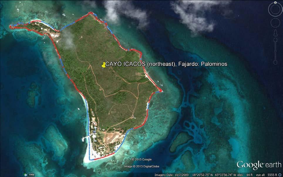
Figure 3. An example of shoreline change analysis output for Isla Palominos. The data are plotted on Google Earth. Red and blue dots are locations of transects selected within the AMBUR program at 10-meter spacing. Red dots indicate transects with net erosion and blue dots indicate transects with net accretion. Shoreline type is not considered. Tables 6 and 7 give overall shoreline change statistics for the project. See Appendix B for complete set of shoreline change maps.
The shoreline change summary calculations are given in Table 7. AMBUR produces the data based on the individual transects analyzed. Mean shoreline change rate is the overall average of change for all transects on each island. Error margin is maximum of +/- 0.2 m/yr. Percent erosion is the percent of each individual island’s shoreline that is experiencing erosion. Mean erosion rate is the average of just the transects experiencing erosion. Mean accretion rate is the average of just the transects experiencing accretion. Transects are created within AMBUR at 10-meter spacing. Subsequent tables present sorted data by mean shoreline change rate and percent erosion.
Table 3. Shoreline change summary.
Negative rates = erosion, positive rates = accretion
Table 8 shows the study area islands sorted by mean shoreline change rate in meters per year. The greatest shoreline change rate is -0.83 meters/year, exhibited by Cayo Ratones. Many of the islands are very nearly stable. Cayo Ratón. Cayo Santiago, Isla Magueyes, and Isla de Cardona have positive shoreline change rates, that is, accretion. Many of the rates are within the statistical margin of error of +/- 0.2 m/yr.
mean shoreline change rate.
Isla Caja de Muertos
Isla Culebrita
Isla Morrillito
Cayo Río
Isla Magueyes 0.05
Isla de Cardona 0.05
*Rates are in meters/year (negative = erosion and positive = accretion)
Table 9 lists study area islands sorted by percent erosion. That is, what percentage of the shoreline of each island is retreating. The largest percentage of the shoreline exhibiting erosion is 95%, found on Cayo Ratones, Isla de los Palomas, and Isla Morrillito.
Table 5. Study area islands sorted by percent erosion.
Island/Cay % Erosion
Cayo Ratones 95
Isla de los Palomas 95
Isla Morrillito 95
Cayo Icacos 93
Isla Caja de Muertos 85
Cayo Diablo 76
Palominitos 75
Isla de Cabras 75
Isla Culebrita 67
Cayo Río 65
Cayos de Ratones 64
Cayo Algodones 63
Paliminos 63
Isla de Cardona 60
Isla Matei 56
Buck 56
Cayo Santiago 55
Isla Magueyes 51
Cayo Batata 45
Cayo Ratón 42
Table 10 is an area analysis for the study islands, based on the island area as measured by the historical shoreline versus the modern shoreline. Accretion area is calculated from every instance where the modern shoreline moved seaward of the historical shoreline. Conversely, the erosion area is calculated from every instance where the modern shoreline moved landward of the historical shoreline. Percent erosion is erosion area compared to historical area. Isla Caja de Muertos is the largest island in the study area with an area of 1,479,280 m 2 (148 ha,1.48 km2). The smallest study island is Palominitos at only 2,132 m 2 (0.21 ha). Palominos has been dominated by erosion
Table 6. Area analysis for islands in the study. Calculated from modern shoreline. Negative numbers indicate erosion.