FINAL REPORT
September 2, 2005
Heavy metals and biomarker toxicity assays in Jobos Bay
National Estuarine Research Reserve
Submitted to:
Sea Grant College Program University of Puerto Rico-Mayagüez
Jessica X. Aldarondo1, Leslie A. Acevedo-Marín1, Sahily González-Crespo1, Enixy Collado2 , Miguel P. Sastre2 , Fatin Samara3, Imar Mansilla-Rivera1, and Carlos J. Rodríguez-Sierra1
1Department of Environmental Health, Graduate School of Public Health, Medical Sciences Campus, University of Puerto Rico, San Juan, Puerto Rico, 00936
2Department of Biology, University of Puerto Rico at Humacao,Humacao, Puerto Rico, 00791
3Department of Chemistry, University at Buffalo, Buffalo, NY 14260
1. Introduction
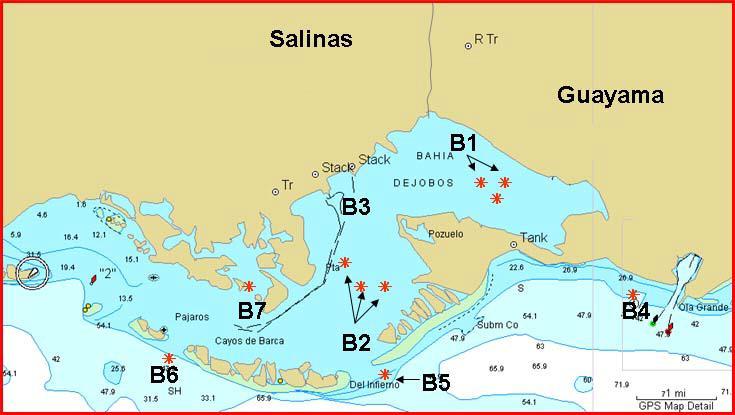
Jobos Bay National Estuarine Research Reserve (JBNERR), comprising an area of 2,800 acres, is located in the south coast of Puerto Rico within the Guayama and Salinas municipalities (Figure 1). JBNERR is the second largest and most important estuary system on the Island supporting a great diversity of fauna and flora (DNER, 2000). Important habitats to wildlife living within the JBNERR limits include coral reefs, extensive seagrass beds, sand beaches, mangrove cays and inland forests, as well as lagoon areas like Mar Negro. Endangered species such as the West Indian manatee, hawksbill and green sea turtles, the brown pelican and the yellow shouldered blackbird live within JBNERR. Areas around JBNERR have undergone significant agricultural and industrial development (DNER, 2000). A number of pesticides and fertilizers were applied to soils on a regular basis to sustain (principally) corn and fruits on agricultural land located to the north of JBNERR. Examples of industrial facilities located in the vicinity of JBNERR included an oil refinery, pharmaceutical plants, a tire recycling center, a solid waste landfill, and a thermoelectric power plant. JBNERR represents a typical tropical Caribbean estuarine system that could serve as a model for coastal management practices in other Caribbean countries. However, since its inception in 1981, little research activity on the environmental quality of JBNERR has been conducted, especially in Jobos Bay. Jobos Bay, with a surface area of 11km2, is a semi-closed aquatic environment, receiving an annual submerged water flow input of approximately 13,000 acres-feet (1.6x10⁷m3) which also comes from streams, rain, and irrigation (DNER, 2000). There is an increasing concern that the proximity of agricultural and industrial activities taking place near the JBNERR could result in undue pressure on this fragile ecosystem by toxic chemical pollutants eventually reaching Jobos Bay via surface water runoff, groundwater or by air. For example, on March 20, 2000, more than 20,000 used tires burned from a tire recycling center spewing toxic chemicals to Jobos Bay. Toxic contaminants reaching Jobos Bay could put in jeopardy not only the well being of this valuable natural ecosystem, but also the health of people associated with it (such as fishermen). Inorganic and organic chemicals released into Jobos Bay could accumulate in bottom sediments reaching concentrations higher than in the water column. For example, Acevedo et al. (2000) found significant differences in metal concentrations in water and sediments from San José (SJL) and Joyuda lagoons, with some sediment metal values like Pb showing 60-fold greater concentrations than in water (Table 1).
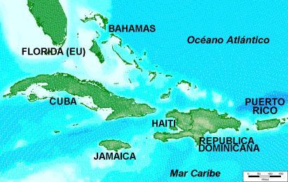
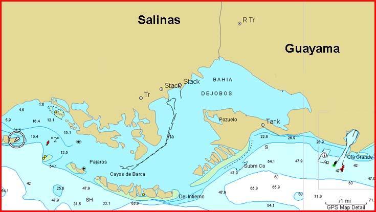
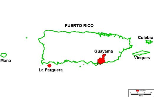
Figure 1. Map of Puerto Rico showing relative locations of JBNERR and reference site of La Parguera.
It is well documented that sediment-bound and water-dissolved chemicals accumulate in biological tissues. On the basis of policyclic aromatic hydrocarbons (PAHs) and halogenated aromatic hydrocarbons concentrations in sediments, Maruya et al. (1997) reported biotasediment accumulation factors for different benthic invertebrate obtaining higher bioaccumulation in clams, while juvenile rainbow trout fish readily accumulated over 50% of pentachlorobenzene after a 6 d incubation (Qiao and Farrell, 1996). Also, the water-filtering false mussel, Mytilopsis domigensis, collected in SJL showed copper (Cu) and zinc (Zn) concentrations as high as 13.9 µg/g dw and 86.3 µg/g dw, respectively (Pérez et al. 2001). Reported concentrations of Cu and Zn in the false mussel (Pérez et al. 2001) were considerably higher than in water samples from SJL (Table 1).
Table 1. Average levels of heavy metals in San José (SJL) and Joyuda lagoons.
(n=11)
From Acevedo et al. (2000). Concentrations units for water are in µg/L, and µg/g dry weight equivalents for sediments. NA, is not analyzed. n, is number of sampling sites.
The bioaccumulation process of anthropogenic chemicals might lead to magnification through the food web, which could increase pollutants levels up to 100-fold, thus, becoming a health hazard to aquatic organisms (Pacirov and Brown 1977; Neff 1978; Bryan and Langston 1992). For instance, organochlorine compounds such as polychlorinated biphenyls (PCBs) have been implicated with reproductive dysfunction with concentrations as low as 1 µg/g body weight in fish (Nirmala, et al., 1999), while PAHs are known mutagens (West et al. 1986; Steinert etal. 1998b). Toxic heavy metals, such as cadmium, copper, and mercury, in aquatic systems are known to cause various adverse effects on fish and shellfish, including premature hatching, growth retardation, developmental abnormalities, and increased mortality (Li et al. 1997; Warnau et al. 1996; Wong et al. 2000). Furthermore, edible fish and shellfish could become a potential health hazard for fish-eating birds such as the endangered brown pelican, and even humans. Fox et al. (1991) reported bill defects in double-crested cormorants from the Great Lakes area that consumed contaminated fish with polyhalogenated aromatic hydrocarbons, while methylmercury, that also accumulate in fish, has been found to be a potent avian embryo and nervous system toxicant (Wolfe et al 1998). Humans are also vulnerable to the neurotoxicant and teratogenic effects of methyl mercury mainly from edible fish and other benthic organisms since terrestrial food is a negligible source for this metal species (D’Itri 1991; Renzoni et al. 1998). A human health risk assessment study for fishermen in Puerto Rico that consumed metal-
contaminated Centropomus spp. (róbalo) fish found muscle-methyl mercury levels that exceeded the United States Environmental Protection Agency chronic reference dose of 0.29 µg/kg/d (Burger et al. 1992). The biomagnification of methyl mercury in the food chain is due to the high lipid solubility, and long biological half-life (Goyer, 1996). National and International Health organizations have establish limits for methyl mercury concentrations as well as for other metals in fish edible muscles to protect against hazardous exposure to humans (Table 2).
Table 2. Health advisory levels of metals (µg/g ww) in edible fish muscle.
Powell et al (1981)
Gonzalez et al. (1991)
Denton and Burdon-Jones (1986)
Diaz et al. (1994)
(1994)
Man So et al. (1999)
Summers et al. (1995)
(As2O3 1.14 (As)
Brasil and Nauen (1983)
Health and Medical Research Council
Spanish Food Directorate tolerance levels
Criterion FDA and Nauen (1983)
Hong Kong Food Regulation
International and FDA (only for Hg) criterion nr, is not reported
Heavy metals are among the aquatic pollutants most frequently detected in different aquatic environmental compartments of estuaries (e.g., sediment, water and biota). Table 1 shows a list of metals commonly studied in aquatic systems by our research group. Metals such as Cd, Pb, and Hg have not known biological functions. Other metals like As, Cu, Se, and Zn are considered essential metals or beneficial only at low concentrations (Goyer, 1996). Factors influencing the toxicity of metals are chemical speciation, interactions with other essential metals, formation of metal-protein or water-dissolved organic matter, age and stage of
development, immune status of the host, and concentration (Goyer, 1996). For instance, metals such as Cd, Cu, and Zn are acutely toxic to fish due to interference with the transport of sodium and calcium (Mattice et al. 1997). The metal Cu has been found to affect the hatching and development of the larvae of estuarine crabs at concentrations as low as 0.5 mg/L (Zapata et al. 2001).
Although metals occur naturally in the environment, human (anthropogenic) activities can augment their natural background concentrations and their potential for health effects (Table 3). It is very important to distinguish the natural versus the anthropogenic contribution of metals in aquatic systems in order to have effective remedial or control actions against environmental contamination by man-made activities. The contribution of anthropogenic sources of metals to coastal and estuarine sediments can be determined using geochemical normalization against a reference element such as iron, aluminum or lithium (Leivuori, 1998). Acevedo et al. (2005) showed that by estimating enrichment factors of metals in SJL and Joyuda lagoon sediments using Fe for normalization, sediment-associated metals in SJL and Joyuda lagoon were of anthropogenic and natural origins, respectively. In addition, utilizing published sediment guideline concentrations (ERM) above which toxic effects in marine organisms are predicted (Long et al. 1995), the author found metal levels (e.g., Hg, Pb, and Zn) in some SJL sampling stations higher than the ERM, associating these concentrations with potential toxic effects to aquatic organisms (Acevedo et al., 2005).
Although the proposed study focuses on the chemical measurement of metals from different environmental compartments of Jobos Bay, there are other hazardous chemicals likely to be present. Since sediments serve both as a sink and a source of anthropogenic pollutants, some of which are mutagenic (e.g., PAHs, organohalogenated pesticides), and at concentrations higher than in other aquatic environmental compartments, it is the most frequently used environmental sample to conduct in vitro toxicity tests such as the mutagenicity assays (Durant and Hemond 1992; Fernández et al. 1992). Mutagenic assays like the Salmonella microsome assay or Ames test assess the ability of environmental pollutants to react with DNA. The Ames test provides the response of the sum of mutagenic chemical constituents present in the sediment sample that chemical analysis alone can not obtain.
Table 3. Heavy metals toxicity characteristics.
METAL ANTHROPOGENIC SOURCES
Arsenic (As) Manufacture of pesticides, herbicides and other agricultural products; smelters
Cadmium (Cd) Electropainting, galvanizing, color pigment for paints and plastics, mining, smelting, batteries
Copper (Cu) Mining, smelting and industrial discharges
Mercury (Hg) Mining, smelting, industrial discharges, burnig coal, refining of petroleum products
CHRONIC EFFECTS
Peripheral vascular disease, neurotoxicity of peripheral and central nervous system, liver, kidney and bladder cancers, leukemia, skin disorders
Chronic obstructive pulmonary disease, emphysema, chronic renal tubular disease
Cirrhosis, cholestatic, inherited disorders of copper metabolism
Central nervous system, neurotoxic effects (vapor Hg, CH3Hg+), mercuric salts: necrosis of kidney and immunological glomerular disease
ACUTE EFFECTS
Fever, anorexia, hepatomegaly, cardiac arrhytmia, death
Nausea, vomiting, abdominal pain
Vomiting, hypotension, coma, jaundice
Acute corrosive bronchitis, intestinal pneumonitis, abdominal cramps, bloody diarrhea and suppression of urine
Lead (Pb) Paints, industrial emissions, leaded-gasoline
Selenium (Se)
Mining and sulfur containing materials
Neurological, neurobehavioral and developmental effects in children, renal effects, reproductive effects
Brittle hair, skin lesion
Zinc (Zn) Industrial mines, batteries Not provided
From Goyer 1996.
Blood pressure
Impaired vision, depressed appetite
Gastrointestinal disease, diarrhea
As already mentioned above, chemical contaminants associated with sediments could mobilize into the water column and become bioavailable to the food web. In vivo assays exist to determine biological damage from exposure to mutagenic chemicals associated to the water column. The highly sensitive alkaline version of the single cell gel electrophoresis (SCGE) or comet assay (Singh 2000) has been used successfully for assessing pollution/environmental stress-induced DNA damage and repair in aquatic organisms (Nascimbeni et al. 1991; Steinert 1996; Steinert et al. 1998a, 1998b; Sastre et al. 2000; Sastre et al. 2001). This technique has been used by Sastre et al. (2000) to study DNA damage in mantle cells of the mussel Musculista senhousia, which is very similar to Brachiodontes exustus (the mussel to be studied) in size and morphology.
The Scorched mussel, Brachiodontes exustus (Mollusca: Mytilidae) is a filter feeder that typically lives in the intertidal zone of marine hard substrates in the Caribbean. This mussel species is often found attached to mangrove roots, pier pilings and other hard substrates at intertidal and/or subtidal levels. This species has been observed in Puerto Rico in all of the above habitats (Sastre et al., 2001). Its distributional range extends from North Carolina to Texas, along the West Indies and from Brazil to Uruguay (Warmke and Abbott 1975). This species can grow to about 20 mm as an adult (Warmke and Abbott 1975), but specimens of over 30 mm in length have been seen in Puerto Rico (Sastre et al., 2001). The fact that B. exustus filters large quantities of water to feed makes it an ideal organism to use as a bioindicator of environmental pollution. The single cell gel electrophoresis (SCGE) or comet assay (Singh, 2000) has been used successfully for assessing pollution-induced DNA damage and repair (Nascimbeni et al., 1991; Sastre et al., 2000, Steinert, 1996; Steinert et al., 1998a, 1998b). Briefly, cells are embedded in agarose gel and placed on a microscope slide, the cells are lysed by detergents and high salt, and the liberated DNA electrophoresed under neutral conditions. When the DNA contains double strand breaks, it migrates from the brightly fluorescent core (or “nucleus”) to the anode, forming an image resembling a comet (when viewed by fluorescent microscopy after staining with a suitable dye). Cells with increased DNA damage display greater fluorescent intensity in the “tail” and longer migration of DNA towards the anode. Singh et al. (1988) introduced a variation of the comet assay where cells are electrophoresed under highly alkaline (pH>13) conditions, and single strand breaks and alkali-labile lesions in the DNA of individual cells can be detected. This variation is much more sensitive to detect DNA damage since almost all genotoxic agents induce, orders of magnitude, more single strand breaks and alkali-labile lesions than double strand breaks (Bernstein and Bernstein, 1991). B. exustus was included in this study mainly because it is relatively abundant at JBNERR, and the comet assay has been used successfully and validated for this species (Sastre et al., 2003).
Although JBNERR was established in 1981, there is a lack of published studies documenting levels of anthropogenic pollutants in Jobos Bay. The hypothesis to be tested is that toxic contaminants, some of which are mutagenic and genotoxic, are present in water and sediments, and are bioaccumulating in aquatic organisms of Jobos Bay due to close proximity to industrial, agricultural, and urban development. This study in JBNERR will determine the extent of
contamination in water, sediments, and biota of Jobos Bay by addressing the following specific objectives:
1) To determine the spatial concentrations of heavy metals in water, sediment, and fish.
2) To determine if the source of metals in sediments is anthropogenic or naturally occurring by normalizing metal concentrations with respect to iron.
3) To determine if sediment-metal concentrations pose a health risk to aquatic organisms using sediment guideline concentrations above which toxic effects in marine organisms are predicted (ERM).
4) To compare metal concentrations in edible fish muscle with levels recommended by local, federal and international health agencies to evaluate the potential health risk to humans.
5) To assess the mutagenicity activity of sediment-accumulated chemicals using the histidine-deficient Salmonella Ames Test.
6) To evaluate the use of the mussel species Brachiodontes exustus as indicator of exposure to water-dissolved carcinogenic contaminants by using the DNA-damage detector known as the Comet assay.
7) To screen for the presence of chemical organics in sediments.
2. Methodology
2.1 Fisherman interview
After explaining the nature of the project and its implications, interested fishermen were asked to sign an informed consent form. Prior to fish sampling, a questionnaire that included a catch record was provided to participating (consented) fishermen to allow us to identify the fish species to be collected based on trophic position (a carnivore), capture frequency and consumption in Jobos Bay.
2.2 Sampling
2.2.1 Fish
After identifying the most common carnivore fish captured by fishermen in Jobos Bay, the sampling of the fish species was conducted with the assistance of local fishermen, and with appropriate permits from the Department of Natural and Environmental Resources. The selection of sampling stations (Figure 2) took into consideration the approximation of potential pollutant sources to Jobos Bay. Fish from the coast of La Parguera was included as a reference site, since this site is located far from agricultural and industrial development. Powder-free rubber gloves were worn during the sampling operation and were changed at different sampling stations. Captured fish were individually placed inside plastic bags, preserved in an ice cooler, and transported to the laboratory for subsequent analyses. Sampling and processing of fish followed USEPA (1996) guidelines.
On December 2003, water and sediment sampling was conducted in the Jobos Bay area, whereas sampling in La Parguera was conducted on January 13, 2004. Superficial sediment and water samples were collected from 14 different stations in the Jobos Bay area (Figure 3), including areas where fish sampling was conducted. Water samples were collected on the same place of sediments. Sampling in La Parguera was conducted on five different sites: Corona Blanca (LP-21) and Turumote (LP-22), where fish sampling was conducted, near the Laurel cay (LP-23), close to the fishing dock (LP-25), and around cays adjacent to the Boquerón State Forest (LP-24).
Figure 3. Water and sediment sampling stations in the Jobos Bay area.
Sediment samples were collected utilizing a Ponar stainless steel dredge (Forestry Suppliers, Inc., Jackson, Mississippi) and placed in a glass tray where sediments were homogenized with a spatula. Sediments for metal analyses were transferred to plastic bags, whereas those for organic chemical analyses were placed in 500-mL wide-mouth amber glass jars with Teflon-lined screw caps. All sediment samples were placed in a cooler with ice, transported to the laboratory and stored either in a freezer at -20oC (metal analyses) or in a refrigerator at 4oC (organic chemical
analyses). After sampling at each station, the dredge, spatula, and glass tray were cleaned to avoid contamination. The cleaning procedure consisted of scrubbing them with a brush, followed by 3 or 4 rinses of ddw, a rinse with 1% hydrochloric acid, several rinses with ddw and a final rinse with 95% ethanol. Excess ethanol was removed with ddw.
Water samples were collected at a one-foot depth with a messenger activated Water Mark horizontal polycarbonate water sampler (Forestry Supplies, Inc., Jackson, Mississippi). Water was transferred to polypropylene bottles (500-mL for Jobos Bay and 1000-mL for La Parguera), acidified to pH < 2 with concentrated HNO3 for preservation, and placed in a cooler with ice to be transported to the laboratory. In-situ water physicochemical characteristics such as station depth, temperature, salinity, conductivity, and dissolved oxygen were measured at every station. For quality control, field blanks and spiked samples were included in each day of sampling. Once in the laboratory, samples were stored in a freezer at -20oC until analysis.
2.2.3 Scorched mussel Brachiodontes exustus
Four sampling sites (Las Mareas, Site 10, the Canal, and Site 9) were selected in JBNERR and a reference site at Papayo (near La Parguera) on the south-western coast of Puerto Rico. Las Mareas is situated near the north-western boundary of JBNERR at a mangrove lagoon connected to Jobos Bay by a narrow mangrove channel (Figure 4). It is the sampling site farthest away from the ocean. The small housing community located along the northern border of the lagoon (Las Mareas community) is not connected to the municipal sewer system, since these facilities are not available in this area. Raw sewage is discharged into septic tanks, which could leach into the lagoon. Site 10 is located at a mangrove lagoon, connected by a mangrove channel to Las Mareas (to the north) and to Jobos Bay (to the south).This lagoon is entirely bordered with mangroves. No houses or other residential structures exist in this area. The Canal sampling site is located at the southern border of the channel that leads to Las Mareas (Figure 4). It is the sampling site closest to the open ocean. Site 9 is located at the eastern boundary of JBNERR, very close to the thermoelectric power plant (Figure 4). Within the power plant boundaries, there are several liquid-retaining ponds, situated very close to this sampling site. Runoff from the power plant may affect water quality at Site 9. The bottom sediments at this site are extraneous to this area. These are mainly composed of a black by-product, produced by a large sugar cane refinery, formerly located to the east of the study area (Central Aguirre).
All B. exustus were hand-picked from submerged Red Mangrove (Rhizophora mangle) roots. Mussels were placed in 1-L plastic bags containing seawater from each sampling site. These were rapidly placed inside a cooler with ice (water temperature in bags approximately 2˚C) and transported to the laboratory within 1.5 h. Study sites in JBNERR were sampled on four occasions: June 27, August 21, November 6, and December 5, 2003. The Papayo reference site (La Parguera) was sampled on one occasion, April 21, 2004. Three mussels from every sampling site in JBNERR were analyzed at each date, and twelve mussels were analyzed from Papayo (La Parguera) on the single sampling occasion.
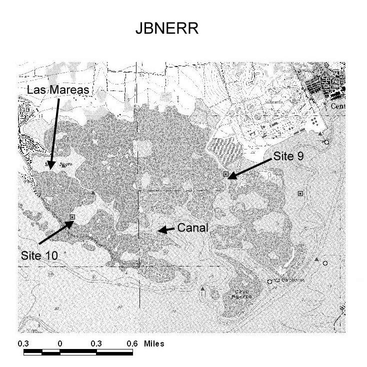
Figure 4. Map of Jobos Bay National Estuarine Research Reserve showing the location of study sites.
2.3 Metals
2.3.1
Fish muscle processing
For fish processing in the laboratory, fish specimens were thawed and length, width, and weight were recorded. Fish samples were rinsed thoroughly with tap water followed by ddw before removing the tissue. Skin with scales was removed with a stainless steel scalpel before removing the muscle. Once removed, muscle tissues were placed inside plastic bags and stored in a freezer at –20 oC. Fish were identified to the species level (Goodson, 1976; Martin and Patus, 1988). Skinless muscle is important for assessing methyl mercury exposure because of its preferential accumulation in muscle, and leaving the skin results in lower Hg concentration in muscle (USEPA, 1996). Scales and skin were removed with a stainless steel knife before removing the muscle. Since nickel and chromium (components of stainless steel) were not being analyzed, the use of a stainless steel knife and scissors was not of concern (USEPA, 1996).
Weights of removed fish muscles were recorded, rinsed with ddw, placed inside plastic bags and stored in a freezer at -20oC.
Water content of fish tissues was determined by drying samples at 60oC, until constant weight. Determination of water content allowed obtaining dry weight (dw) equivalent units for fish tissues. Homogenates of wet muscle were prepared using a ceramic mortar and pestle before microwave assisted digestion.
2.3.2
Sediment processing
Sediment samples were defrosted overnight in a refrigerator and the excess of water was discarded. Sediment samples that were variable in terms of grain-size (stations BJ-1, BJ-2, BJ-4, BJ-8, BJ-13, and LP-24) were homogenized with a sieve of a mesh size of 63 µm. The rest of the sediment samples were homogenized inside the plastic bag prior to digestion.
2.3.3
Digestion
2.3.3.1 Fish and sediment
Digestion of fish muscles for metal extraction started on August 5, 2003. Metals were determined in muscles of Scomberomorus cavalla, Micropogon undulatus, Lutjanus synagris, and Lutjanus analis from Jobos Bay, and in Scomberomorus regalis and Lujanus synagris from La Parguera. Digestion of sediment samples started on June 2004. The digestion methodology in
sediments to analyze As, Cd, Cu, Fe, Pb, Se, Zn was based on the USEPA Method 3051 (USEPA, 1992; CEM, 1994). Except for the analysis of Hg, portions of approximately 0.5 g dry weight equivalents of fish muscles and sediments were digested in a Microwave Sample Preparation oven-model 1000 (CEM Corp, Matthews, NC) with 10 mL of concentrated TraceMetal nitric acid (CEM, 1994). At the end of the digestion, 2 mL of 30% hydrogen peroxide was added and re-digested for 10 additional min (CEM, 1994). After digestion, samples were filtered through a Whatman 41 paper-filter, diluted to 50 mL with ddw, and transferred to 50-mL plastic bottles. The extraction of Hg from muscle tissues and sediments uses a different digestion method, USEPA 7471A, which does not use microwave technology (USEPA, 1992). Briefly, 0.5 g dry weight equivalents of muscle or sediment samples were placed in a 125-mL glass bottle. An acid solution of 5 mL of each concentrated Trace-Metal sulfuric acid and nitric acid was added to glass bottles and heated for 2 min at 95oC in a water bath. The sample was allowed to cool. Then, 30 mL of ddw and 15 mL of potassium permanganate (or until there was no further change in color) was added to each sample. Potassium persulfate (8 mL) was added to each bottle and heated in a water bath at 95C for 1 hr. The sample was diluted with ddw and a hydroxylamine solution (6 mL) was added to each digested sample right before the metal analysis to discolor the solution.
2.3.3.2 Water
Water samples were only digested for the analysis of Hg, As, and Se. The digestion for Hg (Method USEPA 7471A) consisted in transferring 100 mL of water samples to 250-mL glass bottles. An acid solution of 5 mL of Trace Metal-grade sulfuric acid and 2.5 mL Trace Metalgrade nitric acid was added into glass bottles and heated for 2 min at 95oC in a water bath. The sample was allowed to cool. Then, 15 mL of potassium permanganate (or until there was no further change in color) was added to each sample. Potassium persulfate (8 mL) was added to each bottle and heated in a water bath at 95C for 1hr. The sample was diluted with ddw and a hydroxylamine solution (6 mL) was added to each digested sample right before the metal analysis to discolor the solution. The digestion for As and Se consisted of pouring 3 mL of water samples in a 15 mL-plastic bottle. Then, 1 mL of hydrochloric acid and 2 mL of potassium iodide were added to each sample and heated for 45 min at 95oC. The analysis of Cd, Pb, Cu, and Zn did not required digestion of the water samples.
2.3.4 Analysis
A total of seven metals (As, Cd, Cu, Pb, Se, Zn, and Hg) were analyzed for fish muscle, sediment, and water samples. Fe was also analyzed in sediment samples. The analysis of As, Cd, Cu, Pb, Se, Zn, and Fe (only in sediments) in fish muscles and sediments was conducted by a Perkin Elmer Atomic Absorption Spectrophotometer (AAS), Model AAnalyst 800, using modified methods of USEPA (1992) for graphite furnace and direct aspiration flame modes. Hg was analyzed using a flow injection mercury/hydride system (Perkin Elmer – FIAS 400). Se, As, and Hg in water samples were also measured by a Perkin Elmer – FIAS 400 and the rest of the metals in water samples were measured by the AAS mentioned before.
Regression analysis and metal concentrations between sampling sites, were conducted with the non-parametric Mann-Whitney test using the statistical program StatView (SAS Institute Inc., Cary, NC).
2.3.5 Enrichment factors
To assess the anthropogenic contribution of metals to sediments from Jobos Bay and La Parguera areas, enrichment factors (EF) were calculated. Fe was used as the reference element to correct for variable grain size. Iron is often used as a geochemical normalizer for the following reasons (Daskalis and O’Connor, 1995): (1) it is a major component of clay minerals and trace metals are mainly associated to this phase; (2) its geochemistry is similar to that of other trace elements; and (3) its natural concentration in sediments is uniform.
The EF for each sediment sample was calculated using the following equation:
EF = (Me/Fe)sample / (Me/Fe)average shale value where (Me/Fe)sample and (Me/Fe)average shale value are the ratio of the metal concentration (µg/g dw) to Fe levels (% dw) in the sediment sample and in the Earth shale, respectively. The average shale values were taken from Krauskopf and Bird (1995).
2.3.6 Quality assurance
Quality control was achieved by: (i) checking sample containers and reagents, including method blanks to determine background contamination, and (ii) utilizing digested/bench spiked
samples, and standard reference materials (SRM) like SRM 1646A – Estuarine Sediments (National Institutes of Standards and Technology, Gaithersburg, MD) and DORM-2 – Dogfish Muscle (National Research Council, Ontario, Canada), to validate the digestion procedure. In addition, ULTRA-check Blind QC Standards (Fisher Scientific, Pittsburgh, PA) were included to evaluate the AAS calibration curve for each metal.
2.4 Organics (only for sediments)
2.4.1 Sediment processing
Prior to analysis the samples were thawed and air-dried for 48 hrs under dark conditions. The dried samples were ground using a mortar and pestle and passed through a sieve prior to extraction.
2.4.2 Reagents and standards
Dichloromethane (DCM) was purchased from J.T. Baker (Phillipsburg, NJ), acetone from Merck (Whitehouse station, NJ), hexane from EMD (Gibbstown, NJ), and isooctane from VWR International (Bridgeport, NJ). HydromatrixTM for ASE was obtained from Varian (Walnut Creek, CA). Neutral aluminum oxide 90% active (0.063-0.200 mm) was purchased from EM Science (Gibbstown, NJ). A mixture of 16 PAH standard was obtained from Restek (Bellefonte, PA), PAH surrogate (Pyrene-d10 solution) and Internal PAH standard mixture (Acenaphthened10, Phenanthrene-d10 and Chrysene-d12) was obtained from Chemservice (West Chester, PA) (Table 4). PCB standards (PCB 28,52,101,153,138,180,209) were purchased from Accustandard Inc. (New Haven, CT) and (PCB 1,5,29,47,98,154,171,201) from Chemservice (West Chester, PA) (Table 5).
Table 5. Molecular weights and
4,4’, 5,5’ Hexachlorobiphenyl
2,2’, 3,4,4’, 5’ Hexachlorobiphenyl
2,2’, 4,4’, 5,6’Hexachlorobiphenyl
3,3’, 4,4’,
180 2,2’, 3,4,4’, 5,5’ Heptachlorobiphenyl
(394) 201 2,2’, 3,3’, 4,5’, 6,6’Octachlorobiphenyl
209 2,2’, 3,3’, 4,4’, 5,5’, 6,6’ Decachlorobiphenyl
2.4.3
Extraction and cleanup
Twenty grams of dried sediment were mixed with about 10 mL of HydromatrixTM. The mixture was then spiked with 50 µL of pyrene-d10 solution in isooctane (5 µg/mL). The sediment mixture was then loaded into a 33-mL accelerated solvent extraction (ASE) cell fitted with two Whatman circular (1.983-cm diameter) glass microfiber filter from Dionex Corp. (Sunnyvale, CA) and 6-g alumina (activated at 120 °C for 12 h). The cell was fitted initially with one filter, followed by 6 g of alumina, capped with another filter and finally the sediment mixture. The ASE system used was an ASE 200 purchased from Dionex (Sunnyvale, CA, USA). The sediment extraction was performed using a DCM:Hexane (1:1 v/v) mixture as solvent with two cycles at a pressure of 1500 psi and temperature of 100º C. The static time was 5 min, flush volume was 60%, and purge time was 90 sec. The final volume of the extract was approximately 30-40 mL and was carefully evaporated to dryness under a gentle stream of nitrogen and finally brought up to 500-µL with isooctane for analysis by gas chromatography/mass spectrometry (GC/MS) using the selected ion monitoring (SIM) mode (Tables 6 and 7).
2.4.4
Analysis
The concentrated extracts were analyzed using an Agilent 6890 Series gas chromatography system coupled to a MSD 5973 mass spectrometer detector. The GC system was equipped with an HP-5MS capillary column, 0.25 mm i.d., 0.25-µm film thickness, and 30 m length (Hewlett Packard; Houston, TX). The MS was operated under SIM mode using the molecular mass and two additional confirming ions for each analyte (Tables 6 and 7). The temperature program applied in GC was as follows: initial temperature of 110 °C for 5 min, 110-200 °C at 40 °C min-1 for 10 min, 200-280 °C at 7 °C min-1 and 280 °C for 12 min.
Table 6. Ions selected for MS analysis of PCBs.
Analyte
PCB 1 190,188, 152
PCB 5 224, 222,152
PCB 28 258, 256,186
PCB 29 258, 256,186
PCB 47 292, 290, 220
PCB 52 292, 290, 220
PCB 98 326, 324, 256
PCB 101 326, 324, 256
PCB 138 362, 360, 290
PCB 153 362, 360, 290
PCB 154 362, 360, 290
PCB 171 396, 394, 324
PCB 180 396, 394, 324
PCB 201 430, 428, 360
PCB 209 498, 428, 356
Table 7. Ions selected for MS analysis of PAHs.
Analyte
Acenaphthylene
Acenaphthene
Acenaphthene d-10
Anthracene
Benzo[a]anthracene
Benzo[b]fluoranthene
Benzo[k]fluoranthene
Benzo[g,h,I]perylene
Benzo[a]pyrene
Dibenzo[a,h]anthracene
2.4.5
Quality assurance
The extraction recoveries were obtained using the surrogate standard (pyrene-d10) that was added to the sediment samples prior to extraction and were used to correct for the PAH and PCB concentration. Deuterated PAHs (Acenaphthene d-10, Phenanthrene d-10 and Chrysene d-12) and PCB 209 were used as internal standards for PAHs and PCBs respectively, and the deuterated PAH with the retention time closest to a target analyte was used in constructing a calibration curve for that particular compound. Procedural blanks were run with each batch of samples (10 samples per bacth) and were taken through all phases of the analytical procedure. Quantification was based on the base peak, and positive identification was confirmed using the presence of two confirming ions at the area ratios within ±10% variation. Retention time shifts in the chromatogram were corrected using the internal standards, and positive confirmation of the analyte was based in an agreement within ±0.2 min of the expected retention time.
2.5 Mutagenesis assay or Ames test in sediments
2.5.1 Sediment extraction
A portion of 10 g of sediment sample was place inside Teflon vessels with 30 mL of a mixture of hexane:acetone (1:1). This solvent mixture proportion is recommended by the United States Environmental Protection Agency (USEPA) for solid materials because it efficiently extracts polar and non-polar compounds, while generating less toxic waste than dichloromethane (USEPA, 1992). The extraction was conducted with a MSP-1000 microwave sample preparation system (CEM Corp., Matthews, NC) according to the method of López-Avila et al. (1994). Table 8 summarizes the conditions for each extraction technique.
Table 8. Extraction conditions for the MSP-1000.
(stage 1)
(stage 2)
For quality control, laboratory blanks consisted of Teflon vessels with 30-mL extraction solvent but with no sediment samples. In addition, a standard reference material (SRM) 1941b,
Organics in Marine Sediment (National Institute of Standards and Technology, Gaitherburg, MD) was included in the assay. Sediment extracts were transferred into 250-mL rounded bottom flasks. Each sample was reduced to approximately 1 mL using a rotatory evaporator at 50oC, filtered through a 0.45 m-PTFE filter, and collected in 15-mL borosilicate centrifuge tubes. Extracts were further concentrated to 500 µL under nitrogen, and then transferred to 2-mL preweighed amber vials. Sample extracts in 2-mL vials were nitrogen-evaporated to dryness, weighted and reconstituted with 600 µL (100% DMSO, Sigma, Saint Louis) for mutagenesis analysis.
2.5.2 Salmonella strains
TA 98 and TA 100 (Table 9), were inoculated on a 50-mL Falcon tubes with 10-mL of nutrient broth (Fisher Scientific) supplemented with 25 µg/mL of Ampicillin (Sigma, Saint Louis), and grown at 37º C, 200 rpm, for 16 hr in an environment incubator shaker. A blank and positive control was included for each strain: 2-nitrofluorene (Moltox, North Carolina) for TA 98 (2.5 µg per plate) and sodium azide (Sigma, Saint Louis) for TA 100, (2.5 µg per plate) and 2aminoanthracene (Aldrich, Saint Louis) for both strains with S9 (1.25 µg per plate). Six different concentrations were assayed per extract (15, 20, 30, 35, 40, 50 µg per plate) in three replicate plates. The reagents were added in 100 x 13 mm glass tubes previously labeled in the following order: 200 µL of the phosphate buffer pH 7.4 or 10 % S9 (metabolic activation; a 10 % S-9 mix contains, per 100 mL: 10 mL S-9 fraction, 0.5 mM glucose-6-phosphate, 0.4 mM
NADP, 0.8 mmol MgCl2 , 3.3 mM KCl and 10 mM sodium phosphate pH 7.4), the sediment extract, and the cells. The S9 consists of a solution of rat microsomes utilized in the Ames test to detect mutagenic metabolites contained in the sample. Aliquots of 100 µL and 50 µL of TA 98 and TA 100 cultures per tube were used, respectively, and incubated at 37º C in a shaker waterbath (Shaking Waterbath 25, Fisher Scientific) at 45 rpm, for 20 min. Aliquots of 2 mL of molten top agar (0.6 % Bacto-Agar, 0.6 % NaCl, 0.5 mM Biotin/Histidine) were poured onto the surface of GM plates (1.5% Bacto-Agar, 0.5% Glucose, 1X Vogel-Bonner salts). When the top agar has hardened, plates were inverted and placed in a 37º C temperature incubator (Isotemp Incubator, Fisher Scientific) for 48-72 hr. Colonies were counted manually and results expressed as the number of revertant colonies per plate (Maron and Ames, 1983; Claxton et.al., 1987; Gatehouse et.al., 1994; Reed et al., 1999; Mortelmans, et.al., 2000).
Table 9. Characteristics of the Ames assay test strains.
MUTATION
STRAIN
RFA1 UVRB2 HIS3
SPECIFICITY3
TA 98 + - hisD3052 Frame shift
TA100 + - hisG46 Base-pair substitution
1 causes partial loss of the bacteria’s lipopolysaccharide barrier
2 causes deletion of a gene coding for the DNA excision repair system
3 mutation at the histidine operon (Mortelmans et.al., 2000)
SPONTANEOUS REVERTANTS
20 - 50
75 - 200
2.5.3
Spike assay
A spike assay was performed with BJ-14 sediment extract for both strains in the presence and absence of S9 in order to determine if the matrix of the sediment extract interfere with the mutagenicity response. The method utilized was similar to the one previously described. The spike assay consisted in adding positive controls: 2-nitrofluorene (Moltox, North Carolina) for TA 98 (2.5 µg per plate) and sodium azide (Sigma, Saint Louis) for TA 100, (2.5 µg per plate) and 2-aminoanthracene (Aldrich, Saint Louis) for both strain with S9 (1.25 µg per plate), with five different concentrations of the sediment extract (20, 30, 35, 40, 50 µg per plate) in triplicate plates. A solvent control for the positive controls was assayed in duplicate plates consisting in 5.0 µl 100 % acetone for TA 98, 5.0 µl of 10 mM sodium phosphate, pH 7.4, for TA 100 and 5.0 µl of 100% DMSO for both strain in the presence of S9 mix. The results were expressed as the number of revertants colonies per plate.
2.5.4 Data analysis
Means and standard deviations of the number of colonies per plate were calculated from three replicate plates using the Microsoft Excel program. Test results were categorized as noeffect, toxic and mutagenic. Plates were scored as mutagenic if average revertants on sediment extract exposed plates were equal or greater to two times the average number of spontaneous revertants on the solvent control plates (0.00 µg/plate). Plates were scored as toxic if mean revertant values on extract exposed plates were less than half mean spontaneous revertants on solvent control plates (0.00 µg sediment extract per plate). Those plates that were neither identified as mutagenic or toxic were scored as no-effect.
For those plates were the number of revertants colonies were suspected as extreme values, the statistical treatment for outlier rejection, the Dixon’s “Q” test, was used at the 95% confidence level (Rorabacher, 1991).
2.6 Single cell gel electrophoresis (SCGE)/comet assay
2.6.1 Water physical-chemical parameters
Temperaure, salinity, dissolved oxygen, pH and turbidity at sampling sites 9 and 10 (Figure 4) were monitored using YSI model 6000 dataloggers. All paramenters were recorded every 30 min. Data loggers were positioned at approximately 0.75 meters below mean low water. Sites 9 and 10, among others, are monitored continuously by the JBNERR, as part of their Water Quality Metadata program.
2.6.2 Preparation of cell suspensions
Mantle tissue from one valve of B. exustus were removed with a stainless steel microdissection scissor while viewing through a Nikon Model SMZ-2T stereomicroscope, and inserted in 1.5 mL microcentrifuge tubes containing 900 µL filtered seawater (Millipore HA type filter, 0.2 µm retention size). Contents were homogenized for one min using a Kontes pellet pestle motor. A 200 µL aliquot was transferred into another microcentrifuge tube containing 800 µL filtered seawater while kept on ice.
2.6.3 Comet assay
The alkaline version of the single cell gel electrophoresisis (SCGE) or comet assay was performed according to a modification of the technique described by Steinert et al. (1998a). Cell suspensions were spun down in a microcentrifuge at 2000 g for 2 min. The supernatant was discarded and the pellet resuspended in 50-400 µL KLMA (0.65% FisherBiotech low melting temperature DNA grade agarose in Kenney's salt solution, consisting of 0.4M NaCl, 9mM KCl, 0.7mM K2 HPO4, and 2mM NaHCO3, pH 7.5) at 36 ºC. The volume of KLMA depended on cell density, larger pellets being resuspended in larger volumes. Fifty µL of the cell suspension were transfered on slides (duplicate slides for each mussel) previously coated with 1% normal melting temperature agarose (FisherBiotech, low EEO agarose) in TAE (40 mM Tris-acetate, 1 mM EDTA, pH 7.5). These were allowed to gel on a stainless steel tray placed over ice, and top-
coated with 50 µL KLMA. Slides were placed in Coplin jars filled with lysing solution, 2.5 M NaCl, 10 mM Tris, 0.1 M EDTA, 1% Triton X-100 and 10% DMSO, pH 10.0, and incubated at 4ºC for 2 hr.
After lysis the slides were transferred to Coplin jars filled with distilled water and washed 3 times for 3 min in order to remove excess salts. Slides were then placed in a submarine gel electrophoresis chamber filled with alkaline electrophoresis buffer (300 mM NaOH, 1mM EDTA), and DNA that were allowed to unwind for 15 min. After unwinding, electrophoresis was performed at a constant voltage of 0.4 V/cm for 1 h. The slides were neutralized by three 2-min rinses in 0.4 M Tris; and dehidrated by a 5 min rinse in reagent alcohol (Fisher Scientific). After neutralization, slides were dried at room temperature. The complete comet assay procedure was performed the same day samples were taken.
2.6.4 Slide examination and scoring method
The slides were stained with 37 µL of YOYO-1 (Molecular Probes) and examined under a Nikon Eclipse 600 epifluorescent microscope using a B-2A filter cube (excitation filter 450-490 nm blue light, barrier filter 520 nm) at 400 magnification. A visual scoring method was used to classify DNA damage. Cells were classified into one of five categories according to tail intensity (from lowest damage, 1; to maximally damaged, 5). In order to identify damage, images of B. exustus mantle cells exposed to hydrogen peroxide belonging to categories 1 - 5 were printed and used as references. These were chosen in accord with damage categories observed in published photos of a similar scoring technique (Collins and Dušinská, 2002). The technique used by Collins et al. (1993, 1995) and Collins and Dušinská (2002) was similar in using categories, but their values ranged from 0 (not damaged) to 4 (highest damaged). At least 200 “comets” were scored visually per slide.
A DNA damage index was calculated using a modification of the weighted average (Sokal and Rohlf, 1995):
DNA Damage Index = RN/ N where R = damage category (from 1-5); and N = the number of cells belonging to each damage category. According to Kobayashi et al. (1995), the visual scoring method can be as effective as software based scoring. The relationship between the DNA Damage Index and % DNA in the tail and head has already been reported elsewhere for B. exustus (Sastre et al. 2003).
2.6.5 Data analysis
Microsoft Excel was used to organize data from all cells, calculate DNA damage indices and compute descriptive statistics. Stat View version 4.5 software (Abacus Concepts, 1996) was used to calculate a nonparametric Friedman Test among sites (treatments) and sampling dates (blocks) (Sokal and Rohlf, 1995). All probabilites ≤ 0.05 were considered significant.
3. Results and Discussion
3.1 Fish
3.1.1 Collection
From May to June of 2003, the fishing activity took place in the Jobos Bay area (Figure 2). A total of 86 fish specimens comprising eight different fish species and five families were captured from seven areas (stations). In stations B1, B2, B3 (all three located inside the bay), and B7 (Mar Negro) most fish species collected were Scomberomorus cavalla (“sierra”) and Micropogon undulatus (“roncón”), while in B4, B5, and B6, Lutjanus synagris (“arrayado”) predominated followed by Lutjanus analis (“sama”) (Table 10). Four additional fish species were captured but their count was limited to two or less. Stations B1, B2, B3, and B7 are characterized by muddy bottoms, ideal sites for Micropogon undulatus that feed on crustaceans, mollusks and small fish (Martin and Patus, 1988). According to fisher’s accounts from Aguirre, Scomberomorus cavalla is a very common fish species that enter Jobos Bay to feed on smaller fish (e.g., sardines). These two fish species are ideal for a monitoring program on tissue contaminants in estuarine systems because are a bottom feeder and a pelagic fish species. Metal levels in muscle tissues of two common carnivorous coastal species from the area, Lutjanus synagris and Lutjanus analis, were also determined for comparison among species.
Table 10. Collected fish species in the Jobos Bay area.
analis
saurus
Similarly, in coastal waters of La Parguera, a total of 34 fish specimens were captured on July 30 and 31 of 2003 from areas known by local fishermen as "Corona Blanca", near "Enriquez" cays and in the "Turumote". These fishing places were located in open water, more than 1.7 km from the coastline of La Parguera (map not shown). Fish species collected included Scomberomorus regalis ("alasana o sierra"), Lutjanus synagris ("arrayado"), Lutjanus spp. ("pargo"), Haemulon spp. ("cachicata"), Sparisoma spp. ("loro"), and Caranx ruber ("cojinúa") (Table 11) Fish from La Parguera were included as reference samples to compare metal levels with those observed in fish species from Jobos Bay and adjacent areas. Except for Lutjanus synagris, other fish species collected in La Parguera differed from fish species captured in the Jobos Bay area. For instance, although Scomberomorus spp. was found in both sampling sites, the species captured were different (Tables 10 and 11). Micropogon undulatus was not a common fish species on fished areas from La Parguera because sandy bottom floors, instead of muddy, predominated. As already mentioned, M. undulatus inhabits muddy bottom aquatic environments.
Table 11. Fish species collected in La Parguera.
Species
Scomberomorus regalis alasana / sierra 10
3.1.2 Metals in fish tissue
In terms of quality control, percent recoveries from spiked blanks and standard reference materials (SRM) of digestions for fish muscle tissues are presented in Table 12. Average percent recoveries of metals analyzed from spiked blanks varied from 89-100%, and those from the SRM DORM-2 dogfish muscle ranged from 81-103%. Metal concentrations in muscle tissues of four edible fish species from the Jobos Bay area and two fish species from La Parguera area are presented in Tables 13 and 14, respectively. For comparison purposes between fish species for each site, the overall metal concentrations in muscle tissue was used as shown in Table 14 (La Parguera), and Figures 5 and 6 (Jobos Bay). Water content in muscle tissues varied from 77% to 80%.
Table 12. Average percent recoveries from spiked blanks of muscle digestions and the standard reference material DORM2-dogfish muscle.
Spiked Blank
= 16
16
= 16
n = 16 n = 16
= 10
= 16
n = 16 n = 17
stdv = standard deviation; n = number of samples included in average, NA = not available
Table 13. Metal concentrations (µg/g ww) in muscle tissues of fish from the Jobos Bay area.
Species (common name)
Scomberomorus cavalla (sierra) B1 mean ±
n=6
n=14*
*n = 13 for the determination of zinc
n = number of individuals analyzed, se = standard error, MRL = minimum reporting limit of the AAS assuming no matrix interference
Table 13 (cont). Metal concentrations (µg/g ww) in muscle tissues of fish from the Jobos Bay area.
Species (common name)
Micropogon undulatus (roncón)
n=4 B7 mean
n = number of individuals analyzed, se = standard error, MRL = minimum reporting limit of the AAS assuming no matrix interference
Table 13 (cont). Metal concentrations (µg/g ww) in muscle tissues of fish from the Jobos Bay area.
Species (common name)
Lutjanus synagris (arrayado)
B4 mean
B6
n = number of individuals analyzed, se = standard error, MRL = minimum reporting limit of the AAS assuming no matrix interference
Table 13 (cont). Metal concentrations (µg/g ww) in muscle tissues of fish from the Jobos Bay area.
Species (common name)
Lutjanus analis (sama)
n=2
n=5
n=4
n=11
number
Table 14. Metal concentrations (µg/g ww) in muscle tissues of two fish species from La Parguera area.
Species (common name)
Scomberomorus regalis (sierra) mean
n=10
Lutjanus synagris (arrayado)
n=8
n = number of individuals analyzed, se = standard error, MRL = minimum reporting limit of the AAS assuming no matrix interference; *significant at p <0.05 using Mann-Whitney test
Figure 5. Overall average
concentration of metals (µg/g ww) ± standard error in muscle tissues of four fish species from the Jobos Bay area. Different letters denote statistical significance (p<0.05) using the MannWhitney test. n is the number of individual specimens.
Figure 6. Overall average concentration of metals (µg/g ww) ± standard error in muscle tissues of four fish species from the Jobos Bay area. Different letters denote statistical significance (p<0.05) using the Mann-Whitney test. *n=13 for Zn in muscle tissue.
Overall average As concentrations in the four fish species collected from the Jobos Bay area ranged from 0.74 µg/g ww to 2.49 µg/g ww (Table 13). Levels of As were significantly higher in "arrayado" in comparison with the other three fish species (Figure 5). In contrast, "sierra” obtained significantly higher overall average concentrations of Cu (0.25 µg/g ww) and Hg (0.26 µg/g ww), while "roncón” obtained higher levels for Se (0.38 µg/g ww) (Figures 5 and 6). Zn was found to be significantly higher in "sierra" (3.35 µg/g ww) than in "arrayado" (2.70 µg/g ww) and "roncón" (2.65 µg/g ww), but not with "sama" (2.83 µg/g ww). Pb and Cd were detected below the minimum reporting limit.
As it was observed in Jobos Bay (Figure 6), in La Parguera muscle tissues of "arrayado" showed significantly higher overall average concentrations of As than "sierra" (Table 14). In addition, Cu and Zn displayed significantly higher concentrations in "sierra" from La Parguera than in "arrayado" (Table 14). In contrast, Hg concentrations in muscle tissue of "sierra" fish from La Parguera were significantly lower than in "arrayado". Opposite results were obtained with Hg for this two fish species collected in the Jobos Bay area (Figure 6). No statistical differences were observed with Se, while Cd and Pb were below the minimum reporting limit.
Simple linear correlation analyses were used for the log transformed metal concentration (µg/g ww) in muscle tissues and fish body length (cm) for individual and combined sampling sites (Table 15). Correlations of muscle metal concentrations versus fish body size have been used to predict fish size limits to protect human health and determine bioaccumulation, especially for Hg (Chvojka, 1988; Chvojka et al., 1990; Law and Singh, 1991; Díaz et al., 1994; J rgensen and Pedersen, 1994; Joiris et al., 1999; Rodríguez-Sierra and Jiménez, 2002; Sager, 2004). For fish species from the Jobos Bay area, significant statistical relationships were observed for Hg, Se, and As, while for La Parguera, only As, Hg and Zn correlated with fish lenght (Table 15). "Arrayado" from Jobos Bay and La Parguera obtained positive linear relationships for Hg. The same trend with Hg was observed with "sama". Surprisingly, "sierra" from neither of the sampling sites showed a significant relationship between body size and Hg concentrations, even when this fish species obtained higher Hg levels in Jobos Bay (Table 15 and Figure 6). Frequently, Hg levels in muscle tissues exhibit a positive statistical relationship with body size because of limited excretion (Powell et al., 1981). The lack of correlation between Hg
in muscle tissues and body length of "sierra" was probably due to the limited fish length distribution for each site. "Sierra" from Jobos Bay were significantly larger (55.2 cm) than "sierra" from La Parguera (41.9 cm). Combining "sierra" from both sites, a statistical positive relationship was obtained between body length and Hg concentrations (Table 15). Arsenic was positively associated to body length for "sierra" from La Parguera, but negatively associated in "arrayado" from the Jobos Bay area. This same significant negative relationship, although with lower correlation coefficient (a weak association), was obtained for As and Cu when combining fish lenghts of "arrayado" from both sampling sites. Negative association of tissue-metal concentration and fish body length reflects a lack of metal bioaccumulation. An inverse significant relationship was also observed with Zn in "sierra" fish from La Parguera. Inverse relationship with metals (e.g., Cu and Zn) has been observed in other marine fish species (Powell et al., 1981). Selenium positively correlated with "sierra" length from Jobos Bay, but not for La Parguera or sites combined. No significant association was found between metal concentrations in muscle tissue of "roncón" fish and length possibly due to the limited body size range collected by the gill-net. In summary, metal-fish body length association was variable among fish species and sampling sites. When combining sampling sites for "sierra" and "arrayado", only Hg had consistent significant positive associations with fish length. Mercury is known to bioaccumulate and biomagnify through the food-web because of limited fish body excretion (Powell et al., 1981).
Table 15. Regression equations for metal concentrations (log10) and total length (cm) for fish species from the Jobos Bay and La Parguera areas.
JOBOS BAY
Sierra
(As) = 0.143 - 0.003(L), r2 = 0.023, p = 0.60
(Cu) = -0.47 - 0.002(L), r2 = 0.144, p = 0.181 (Zn) = 0.676 - 0.004(L), r2 = 0.016, p = 0.67
(Se) = -0.752 + 0.004(L), r2 = 0.371, p = 0.021 (Hg) = -0.599 + 2E-4(L), r2 = 1.7E-4, p = 0.96
Roncón
(As) = -0.162 - 0.003(L), r2 = 3.8E-4, p = 0.93
(Cu) = -0.651 - 0.004(L), r2 = 0.003, p = 0.82 (Zn) = 0.404 + 4.5E-4(L), r2 = 3.2E-4, p = 0.94
(Se) = -0.025 - 0.012(L), r2 = 0.077, p = 0.224 (Hg) = -2.48 + 0.041(L), r2 = 0.122, p = 0.120
LA PARGUERA
Sierra
(As) = -0.734 + 0.012(L), r2 = 0.604, p = 0.008 (Cu) = -0.29 - 0.007(L), r2 = 0.318, p = 0.089 (Zn) = 0.96 - 0.009(L), r2 = 0.479, p = 0.027 (Se) = -0.678 + 0.003(L), r2 = 0.274, p = 0.121
(Hg) = -1.446 + 0.011(L), r2 = 0.109, p = 0.353
COMBINED SAMPLING SITES
Sierra
(As) = -0.287 + 0.004(L), r2 = 0.071, p = 0.257 (Cu) = -0.585 - 4.6E-5(L), r2 = 5.3E-5, p= 0.98 (Zn) = 0.181 + 0.007(L), r2 = 0.178, p = 0.064 (Se) = -0.503 - 0.001(L), r2 = 0.037, p = 0.414 (Hg) = -1.639 +0.018(L), r2 = 0.404, p =0.001
3.2 Water
3.2.1 Physico-chemical properties
Arrayado (As) = 1.858 - 0.61(L), r2 = 0.266, p = 0.028 (Cu) = -0.024 - 0.02(L), r2 = 0.200, p = 0.063 (Zn) = 0.768 - 0.013(L), r2 = 0.193, p = 0.068 (Se) = -0.320 - 0.010(L), r2 = 0.084, p = 0.243 (Hg) = -2.185 + 0.051(L), r2 = 0.532, p = 0.001
Sama (As) = -0.76 + 0.019(L), r2 = 0.175, p = 0.201 (Cu) = -0.924 + 0.002(L), r2 = 0.051, p = 0.504 (Zn) = 0.515 - 0.002(L), r2 = 0.032, p = 0.60 (Se) = -0.865 + 0.008(L), r2 = 0.186, p = 0.185 (Hg) = -2.002 + 0.028(L), r2 = 0.643, p = 0.003
Arrayado
(As) = 0.608 - 0.021(L), r2 = 0.247, p= 0.210
(Cu) = -0.55 - 0.011(L), r2 = 0.158, p = 0.330
(Zn) = 0.344 + 0.003(L), r2 = 0.24, p = 0.217
(Se) = -0.13 - 0.022(L), r2 = 0.155, p = 0.334
(Hg) = -1.129 + 0.016(L), r2 = 0.771, p = 0.004
Arrayado
(As) = 1.157 - 0.037(L), r2 = 0.193, p = 0.025 (Cu) = -0.406 - 0.014(L), r2 = 0.165, p = 0.039 (Zn) = 0.497 - 0.003(L), r2 = 0.026, p = 0.432 (Se) = -0.132 - 0.019(L), r2 = 0.129, p = 0.072
(Hg) = -1.57 + 0.029(L), r2 = 0.366, p = 0.001
Physico-chemical properties of water samples from the Jobos Bay area and La Parguera are presented in Tables 16 and 17, respectively. Although station depths in the Jobos Bay area were variable (from 1.8 m in station BJ-2 to 13.8 m in BJ-10), dissolved oxygen (4.0 mg/L – 5.6 mg/L) and temperature (26.5oC – 27.8oC) were similar in all stations. In addition, most of the samples obtained measured salinities between 31 parts per thousand (ppt) to 33 ppt (with the
exception of station BJ-8 which obtained a salinity of 25 ppt). Water samples from La Parguera obtained average higher levels of dissolved oxygen (7.0 mg/L ± 1.5 mg/L) and lower values of salinity (30.7 ppt ± 0.4 ppt). Station depths in La Parguera ranged from 1.4 in LP-24 to 7.6 m in LP-21.
Table 16. Physico-chemical properties of water samples from the Jobos Bay area.
Table 17. Physicochemical properties of water samples from La Parguera.
3.2.2 Metal concentrations
A total of seven metals (As, Pb, Cd, Cu, Hg, Se, and Zn) were analyzed in all water samples from Jobos Bay (14 stations) and La Parguera (5 stations) areas. Levels of Hg, Se and Zn in each station of both areas were below the minimum reporting limits of the instrument (0.5 µg/L for Hg and Se, and 20 µg/L for Zn). Values obtained for As, Pb, Cd, and Cu at each station are shown in Figures 7 to 10. For most metals, few differences in metal levels were observed among stations in each site and between sites. Overall average metal concentrations in Jobos Bay and La Parguera are presented in Table 18.
Levels of As in Jobos Bay ranged from 0.81 µg/L in station BJ-9 to 1.37 µg/L in stations BJ5 and BJ-8 (Figure 7). In La Parguera, As concentrations varied from 1.01 to 1.35 µg/L. When comparing average As concentrations (µg/L) between Jobos Bay (1.07 ± 0.03) and La Parguera (1.15 ± 0.05), no statistical differences were observed (Table 18). The highest concentration value for Pb was obtained in station BJ-12 (7.70 µg/L) whereas the lowest (1.29 µg/L) was measured in station BJ-8 (Figure 7). Average Pb values (µg/L) in Jobos Bay (5.4 ± 0.5) and La Parguera (6.2 ± 0.1) were similar. Cadmium levels (µg/L) were statistically higher in Jobos Bay (0.39 ± 0.07) than in La Parguera (0.23 ± 0.02) (Table 18). On the contrary, Cu levels (µg/L) were lower in the Jobos Bay area (0.8 ± 0.1) when compared with La Parguera (2.0 ± 0.4).
When comparing metal levels in water samples of Jobos Bay and La Parguera areas with levels obtained in two other estuarine systems in Puerto Rico (San José Lagoon and Joyuda Lagoon, Acevedo et al., 2000), it can be observed that levels of Hg, Se, and Zn were similar in all four sites (Table 18). Levels of Cd and Cu were lower in Jobos Bay and La Parguera areas than in the two other estuarine systems. As levels were similar to those obtained in San José Lagoon but much lower than levels measured in water samples from Joyuda Lagoon. Levels of Pb in Jobos Bay and La Parguera areas were also much lower than those obtained in Joyuda Lagoon. In the Joyuda Lagoon area are located mineral deposits that are rich in metals (CarvajalZamora et al. 1980), which may explain the observed difference in metal levels in this estuarine system when compared with the other areas in Puerto Rico.
Figure 7. Arsenic concentrations (µg/L) in water samples from the Jobos Bay area (BJ) and La Parguera (LP). Error bars represent standard errors.
Figure 8. Lead concentrations (µg/L) in water samples from the Jobos Bay area (BJ) and La Parguera (LP). Error bars represent standard errors.
0.0
Figure 9. Cadmium concentrations (µg/L) in water samples from the Jobos Bay area (BJ) and La Parguera (LP). Error bars represent standard errors. <MRL = below the minimum reporting limit of the instrument.
Figure 10. Copper concentrations (µg/L) in water samples from the Jobos Bay area (BJ) and La Parguera (LP). Error bars represent standard errors. <MRL = below the minimum reporting limit of the instrument.
Table 18. Average metal concentrations (µg/L) ± standard error in water from the Jobos Bay area (BJ), La Parguera (LP), Joyuda Lagoon (JL), and San José Lagoon (SJL).
n = 14
n = 4
# n = 17
n = number of stations in each site; * = statistical difference between BJ and LP (p<0.05); # = taken from Acevedo 2000
3.3 Sediments
3.3.1 Metals
3.3.1.1 Concentrations
Water content in sediment samples was determined to express metal concentrations on a dry weight basis. Percent of water in sediment samples from the Jobos Bay area ranged from 18.9% in BJ-11 to 87.8% in BJ-8; whereas in La Parguera, water content varied from 29.0% in LP-21 to 77.9% in LP-24. With the exception of sample BJ-5 which was digested only once, and two other samples that were digested in triplicates (BJ-10 and LP-25), the rest of the sediment samples were digested in duplicates for the extraction of metals. Selenium was not analyzed because of the presence of matrix interferences in the samples.
The percent recovery of spiked blanks varied from 83% to 108 %, showing that the laboratory process of the samples did not result on analyte loss (Table 19). On the contrary, low recovery (61% to 75%) was obtained for Pb, Hg, Zn , and Fe from the SRM 1646a estuarine sediment, while better recovery (84% to 95%) was observed for As, Cd and Cu (Table 19). These recoveries suggest that the digestion method was not efficient in recovering all metals from the SRM sediment. However, the reproducibility of the metal concentrations measured in the SRM was good for this digestion method based on the low standard deviations (Table 19).
Table 19. Average percent recoveries from spiked blanks of sediment digestions and the standard reference material NIST 1646a - estuarine sediment.
stdv = standard deviation; n = number of samples included in average, NA = not available
Concentrations of metals in surface sediments from Jobos Bay and La Parguera areas are presented in Table 20. Most of the samples from Jobos Bay and La Parguera areas obtained Hg levels below the minimum reporting limit of the instrument (0.073 µg/g dw). Cadmium concentration values were also low, ranging from 0.01 µg/g dw in various stations of both sites, to 0.2 µg/g dw in stations BJ-8 and LP-24. For the rest of the metals, spatial variations were observed in both sites. For instance, As values (in µg/g dw) in the Jobos Bay area ranged from 8.3 in BJ-14 to 26.6 in station BJ-10. In La Parguera, As concentration values were even more variable, ranging from 0.7 µg/g dw to 30 µg/g dw. Concentration values for Cu in µg/g dw in Jobos Bay varied from 1.6 in BJ-1 to 53 in BJ-3, while in La Parguera concentrations fluctuated from 0.5 (LP-22) to 36 (LP-25).
Although average levels (µg/g dw) of As (17 ± 1), Pb (11 ± 1), Cu (29 ± 3), and Zn (64 ± 6) were higher in sediments from the Jobos Bay area than in those from La Parguera (9 ± 3, 4 ± 1, 14 ± 5, and 28 ± 7, respectively), there was no preferential station for the accumulation of metals in the Jobos Bay area. This may indicate that metals in the Jobos Bay do not come from similar sources. For instance, the highest level of Zn (129 µg/g dw) were found in station BJ-14 possibly from the burning of the former tire recycling plant located in the area. Similarly, the highest levels of Cd (0.21 µg/g dw) were observed in station BJ-8, where human activities from Las Mareas community may be impacting the area. Conversely, in La Parguera, station LP-24 accumulated the highest levels of As, Pb, and Cd, while station LP-25 accumulated higher levels of Cu, Zn, and Hg. Despite these observed patterns, all metals were below the Effects RangeMedian (ERM) value (Table 20), representative of concentrations above which effects frequently occur.
Table 20. Average metal concentrations ± standard error (dry weight basis) in surface sediments from Jobos Bay and La Parguera areas.
JOBOS BAY
n = 2
n = 2
Table 20 (cont). Average metal concentrations ± standard error (dry weight basis) in surface sediments from Jobos Bay and La Parguera areas.
n = 2
n = number of samples analyzed and included in the calculations; NA = not available; MRL = minimum reporting limit of the instrument; se = standard error; * = statistical difference between Jobos Bay and La Parguera sites (p< 0.05); ERM = Effects Range-Median value, representative of concentrations above which effects frequently occurs in aquatic organisms.
Table 21 presents average metal concentrations in sediments from the Jobos Bay area, La Parguera, and two other estuarine systems in Puerto Rico. With the exception of As, metal levels obtained in the Jobos Bay area compare with those obtained in Joyuda Lagoon, a natural reserve. Conversely, their concentrations are much lower than those measured in sediments from San José Lagoon, which is a known metal contaminated system. When compared with the world average shale value, metal levels in Jobos Bay and La Parguera areas were low. This value represents the background concentration of metals in sedimentary rocks formed by clay or argillaceous material worldwide.
Table 21. Average metal concentrations (dw) in sediments from the Jobos Bay area, La Parguera, Joyuda Lagoon, and San José Lagoon.
* = statistical difference between Jobos Bay and La Parguera (p<0.05); # = from Acevedo et al., 2005; ## = from Krauskopf and Bird 1995
3.3.1.2 Enrichment Factors.
Enrichment factors (EF) were calculated to determine the anthropogenic contribution to metal levels in sediments from Jobos Bay and La Parguera areas. EF were interpreted with the following scale (Birch 2003): EF < 1 indicates no enrichment, < 3 indicates minor anthropogenic contribution, 3 – 5 is moderate, 5 – 10 is moderately severe, 10 -25 is severe, 25 –50 is very severe, and > 50 is extremely severe. The anthropogenic contribution to metal levels was not calculated in stations BJ-11, LP-21, LP-22, and LP-23 because Fe levels in these stations were below the minimum reporting limit of the instrument due to coarse-sandy texture of these samples. Sediments with coarse particles like sand are known poor trace metal accumulator resulting in dilution of metal-contaminated fine-grained sediments (Mudroch and Azcue, 1995). EF values for all stations are shown in Figures 11 – 15. In the Jobos Bay area, the only station that showed enrichment (classified as minor) for all metals was BJ-8. This station is located near “Las Mareas”, a fishing village, in “Mar Negro”. This minor anthropogenic contribution observed for all metals (Cd, Pb, Cu, Zn, and As) may indicate that this area is being affected by domestic wastewater discharges or by agricultural activities. Stations BJ-3 and BJ-14 also received minor anthropogenic inputs for most metals except for Cd. These stations are located
nearby a tire recycling center that was burned on March 2000, implying the release of contaminants from this event. Minor enrichment of Zn was observed in most stations except for BJ-7 and BJ-10. Similarly, the anthropogenic input of As into sediments of the Jobos Bay area was observed in all stations, even on a moderate (BJ-5 and BJ-9) or moderately severe (BJ-10) level.
Interestingly, stations LP-24 and LP-25 in La Parguera showed EF for all metals, at least on a minor level. Cu and As were the metals with most anthropogenic inputs, with 3 < EF < 10. LP25 is located near the dock where most boats are maintained and it may be receiving discharges from these activities. However, station LP-24 is the farthest station from the residential area in La Parguera. A previous study (Rodríguez and Jiménez, 2002) revealed that fish collected from this area obtained higher As, Cd and Cu levels than fish collected from San José Lagoon. These results suggest that further studies should be conducted in the area to determine possible sources of metal contamination.
12. Lead enrichment factors in Jobos Bay and La
areas. NA is not available.
14.
available.
is not available.
3.3.2. Organics
A screening organic analysis was conducted for sediments of seven stations of Jobos Bay (BJ-6, BJ-7, BJ-9, BJ-10, BJ-12, BJ-13, and BJ-14) and one station from La Parguera (LP-25) for the presence of seventeen PAHs and fourteen PCB congeners. Within Jobos Bay, spatial variations were observed for PAHs and PCBs in sediments (Tables 22 and 23). In terms of PAHs, station BJ-14 obtained the highest total concentration with 1,986 ng/g followed closely by stations BJ-13 and BJ-9 with 1,007 and 704 ng/g, respectively. Station BJ-14 is located adjacent to the former tire recycling center that burned on March 20, 2000. PAHs are expected to form from the incomplete combustion of the tires resulting in their accumulation in bottom sediments. PAHs from BJ-13 possibly originated from the nearby Pozuelo marina, while PAHs in station BJ-9 is near the thermoelectric plant and may be receiving discharges from this source. Interestingly, sediments from La Parguera (LP-25) obtained the highest concentration of total PCBs. This station in La Parguera is located next to a fishing dock.
3.3.3 Mutagenicity assay
3.3.3.1 Quality control (spontaneous revertants)
The characteristic spontaneous mutant frequency for each strain (TA 98 and TA 100) was determined using the preincubation method previously described in the section of materials and methods. Table 24 shows the mean of spontaneous histidine revertant values per plate with and without metabolic activation (negative control).
When comparing the results shown in Table 24 with those of Mortelmans and Zeiger (2000), the data fit in the range of their results. These control values showed that the genetic integrity of both strains was not compromised and both strains were suitable for the assay.
Table 22. Policyclic aromatic hydrocarborn (PAH) in sediments of the Jobos Bay and La Parguera areas.
Sampling site
Concentrations (ng/g)
Table 23. Polychlorinated biphenyls (PCBs) in sediments of Jobos Bay and La Parguera areas.
Sampling site
Concentrations PCBs (ng/g)
Table 24. Spontaneous histidine-revertant control values* .
NUMBER OF
REVERTANTS
sTRAIN
TA 98
TA 100
WITHOUT S9 WITH S9
25.18 ± 7.08
111.24 ± 30.84
28.00 ± 7.83
129.09 ± 38.51
*Values are expressed as mean with standard deviation.
3.3.3.2 Positive controls
To determine the response of cells to the positive controls (e.g., 2-nitrofluorene, 2aminoanthracene, and sodium azide), the assay was carried out by searching for an optimal doseresponse relationship. For TA 98 and TA 100, 2-nitrofluorene and sodium azide were used at levels of 0, 2.5, and 5.0 µg per plate, respectively, in the absence of the S9 solution. For both strains, 2-aminoanthracene was used at 0, 2.5, and 5.0 µg per plate in the presence of 10% S9 solution (Figures 16 and 17). Amounts of 2.5 µg/plate of 2-nitrofluorene and sodium azide without S9, and 1.25 µg/plate of 2-aminoanthracene with S9 were utilized with sediment extracts of BJ-14, while the SRM 1941b was used to test the assay.
Number of revertans
Number of revertants
Dose response of TA 98 with2-Nitrofluorene
TA 98 (11/29/03)
TA 98 (01/15/04)
Concentration(µg/plate)
Dose response of TA98 with2-Aminoanthracene in presence of S9
TA 98 (01/09/03)
TA 98 (01/15/03)
Figure 16. The dose response for TA 98 with 2-Nitrofluorene and 2-Aminoantracene in presence of 10% S9.
Number of revertants
Dose response of TA 100 withSodiumAzide
Number of revertants
Concentration(µg/plate)
TA 100 (11/29/03)
TA 100 (12/03/03)
TA 100 (01/15/03)
Dose response of TA 100 with 2-Aminoanthracene in presence of S9
TA 100 (12/03/03)
TA 100 (01/09/03)
TA 100 (01/15/03)
Concentration (µg/plate)
Figure 17. The dose response for TA 100 with Sodium Azide and 2-Aminoanthracene in presence of 10% S9.
3.3.3.3
Mutagenicity of sediment extracts
For the Jobos Bay, the mutagenicity assay was performed using sediments from five different sites, BJ-6, BJ-7, BJ-10, BJ-12 and BJ-14, while for La Parguera, LP-21 and LP-25 were included for the assay (Tables 25 and 26). The first site, BJ-6, showed a mutagenictiy response only with TA 100 strain at 15 and 20 µg/ plate without S9, and a toxic effect at 35 and 40 µg/plate. With the TA 98 strain and with S9 for both strains, no effect was detected. BJ-7 showed mutagenicity with TA 100 strain at 15, 20, 30 and 35 µg/ plate without S9, while with S9 it showed mutagenicity at 15 and 20 µg/ plate. TA 98 strain, without S9, presented a mutagenic response at 20 µg/ plate, and a toxic effect for 50 µg/plate without S9. BJ-10 presented a mutagenic response only with TA 100 strain without S9 at 40 µg/ plate. A toxic response was observed with TA 98 strain at 15 and 30 µg/plate without S9 and at 50 µg/plate with S9. For BJ-12 a mutagenic response was detected only with TA 98 strain at 40 µg/ plate without S9. No effect was detected with sediment extracts of BJ-14 when using TA 100 strain with and without S9. In contrast, a mutagenic effect was obtained at 40 µg/plate with TA 98 strain without S9, and a toxic effect at 30 µg/plate without S9, and at 50 µg/plate with S9 for the same strain.
In La Parguera, only TA 98 strain showed mutagenicity a 15 and 30 µg/plate without S9 for LP-25 (Table 26). For LP-21, a toxic effect was obtained at 30, 35 and 50 µg/plate without S9, and at 40 and 50 µg/plate with S9 with the same strain. For TA 100, no response was detected with and without the S9 (Table 26).
For the quality control assay, we detected mutagenicity in TA 100 strain when sodium azide was added at 2.50 µg/plate for the extract (BJ-14) (Table 27). In presence of S9 for a mutagenic effect with the positive control, 2-aminoanthracene was added at 1.25 µg/plate. In the absence of a chemical no effect was detected. For TA 98 strain no response was detected with and without the positive control; in the presence of S9 only with 2-aminoanthracene a mutagenic response was detected (Table 27).
In conclusion, the Ames Salmonella/microsome mutagenicity assay showed mixed results with sediment samples of the Jobos Bay area and La Parguera suggesting the absence or insufficient amount of mutagenic chemical compounds in sediments as to elicit a mutagenic dose-response. Spike experiments with positive controls using sediment extract from BJ-14 showed that the sediment matrix did not interfere with the mutagenicity analysis (Table 27). Table 25. Results showing the standard deviation for the Jobos Bay sites in TA 98 and
TA 100 strains* .
BJ-6
BJ-7 0.00
± 3.51
± 2.89
± 1.41
± 3.46
± 3.21
± 12.02
±11.37
± 0.00
± 2.12
± 2.83 **
± 5.57
± 2.12
± 4.24
± 2.52@
BJ-10 0.00
± 0.00@
± 2.31
± 9.64
± 9.90
BJ-12 0.00
± 2.12
± 0.00@
± 2.08
± 3.46 **
± 19.09
± 4.73
± 2.08
± 2.31
± 26.87**
± 0.00@
± 3.54@
± 4.58
± 2.12
± 7.51
± 5.51
± 4.95
± 3.46
± 4.36
± 2.12
± 3.51
± 3.61
± 1.73
± 2.65
± 2.12
± 8.00
**
±
± 80.61**
± 5.00
±
±
± 1.15
± 1.41
± 1.53 13.33 ± 4.93 16.67 ± 7.23 15.50 ± 6.36 14.67 ± 2.08 14.00 ± 5.29 8.67 ± 2.08@
± 1.15
± 17.62
± 18.73
± 7.07
± 7.07
± 2.83
± 4.24
* Results were expressed as mean of revertants per plate, **mutagenic effect, @ toxic effect.
±
± 21.21
± 14.14
± 18.38
± 13.58
± 14.14
± 15.56
± 0.71
Table 26. Results showing the standard deviation for La Parguera sites with TA 98 and TA 100 strains* Strain
± 10.39
± 13.20
± 3.21
± 0.00@
± 0.00@
± 7.81
± 7.37@
± 7.37
± 3.61
± 3.79
± 1.73
± 1.73@
± 3.00@
*Results were expressed as mean of revertants per plate, **mutagenic effect, @ toxic effect.
Table 27. Results showing the standard deviation for the Jobos Bay site with both strains and the positive controls*
Strain
± 2.83
± 8.00
± 15.31
± 12.02 544.67 ± 122.15**
± 53.74**
817.00 ± 134.35**
671.33 ± 21.94**
± 21.94**
665.00 ± 26.87** * Results were expressed as mean of revertants per plate, ** mutagenic effect, @ toxic effect, 2-AA means 2-aminoanthracene.
± 2.12