Figure 179. Posting showing location of bathymetry and topography values for Charlotte Amalie Bay, St. Thomas, USVI. 115
Figure 180. Depth contour plot of outer computational grid for Charlotte Amalie Bay, St. Thomas. Also shown is the outline of the nested grid. 115
Figure 181. Depth contour for nested computational grid for Charlotte Amalie, St. Thomas. 116
Figure 182. Hs contour plot for Charlotte Amalie, St. Thomas, based on the scenario listed along the top margin of figure. 116
Figure 183. Hs contour plot for (nested) Charlotte Amalie, St. Thomas, based on the scenario listed along the top margin of figure. 117
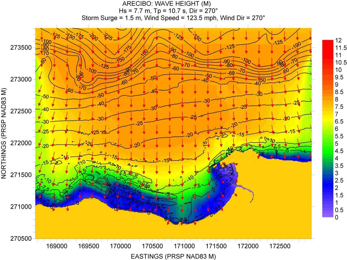
Figure 184. Hs contour plot for Charlotte Amalie, St. Thomas, based on the scenario listed along the top margin of figure. 117
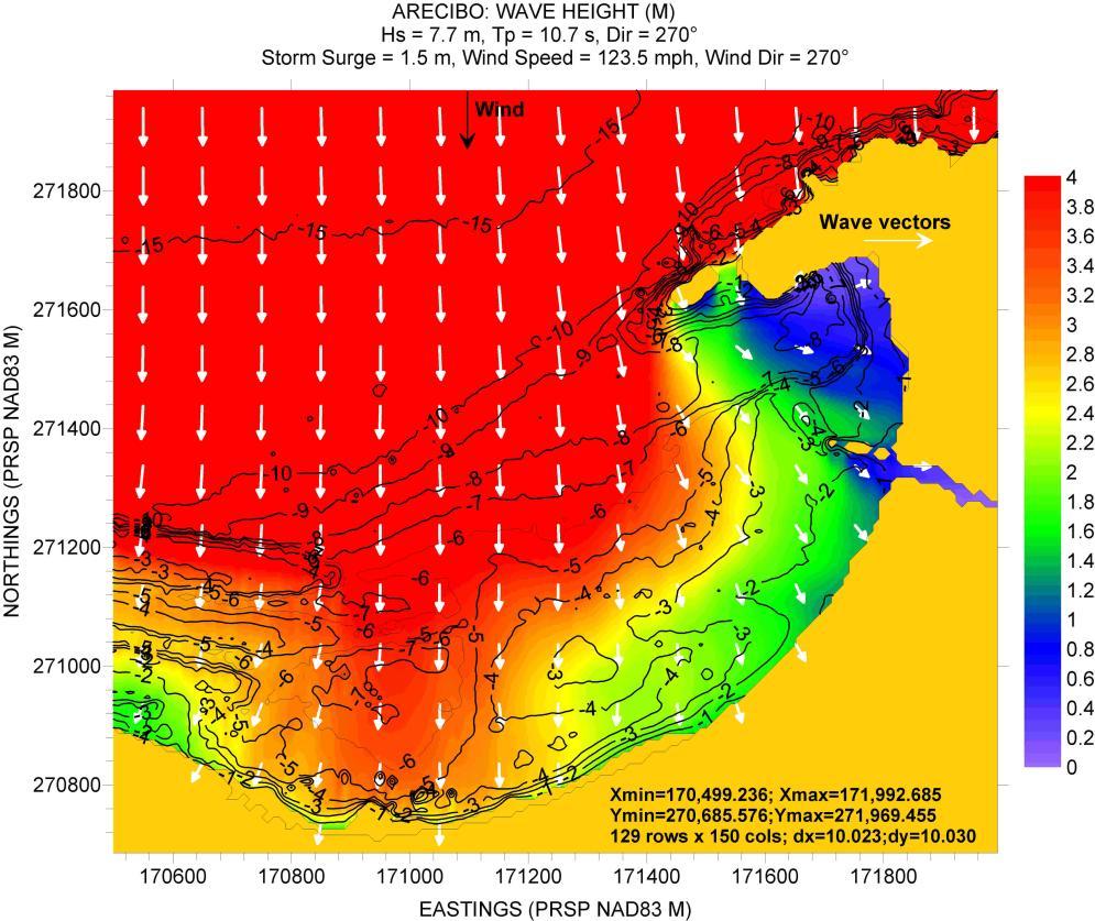
Figure 185. Hs contour plot for (nested) Charlotte Amalie, St. Thomas, based on the scenario listed along the top margin of figure. 118
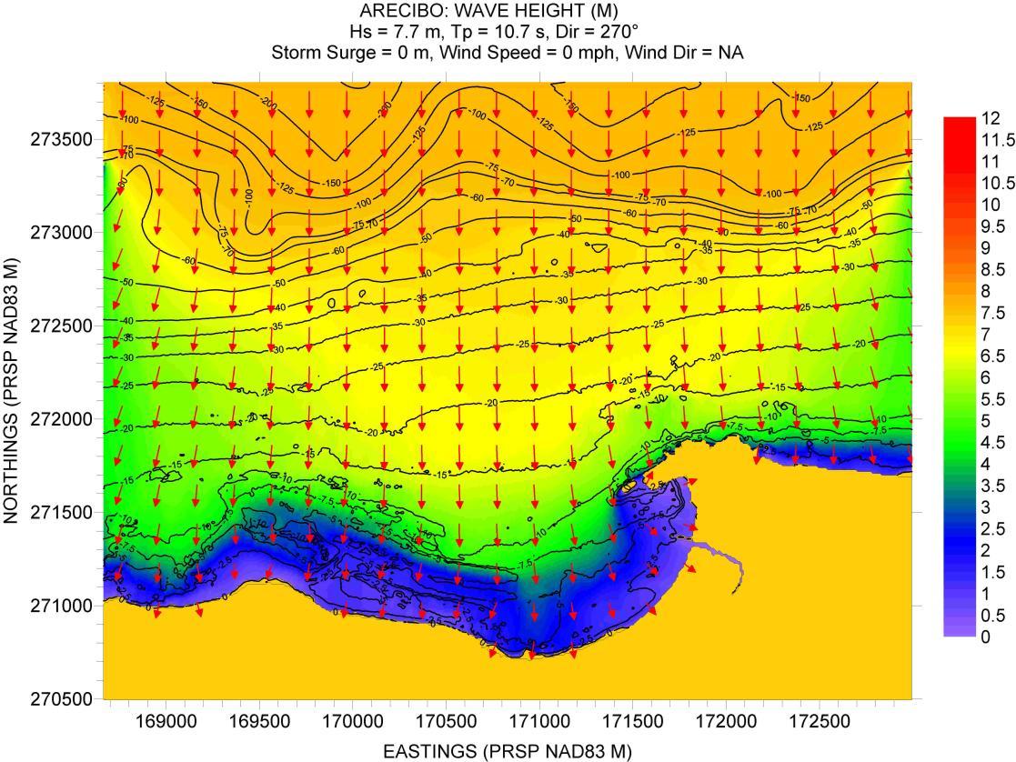
Figure 186. Hs contour plot for Charlotte Amalie, St. Thomas, based on the scenario listed along the top margin of figure. 118
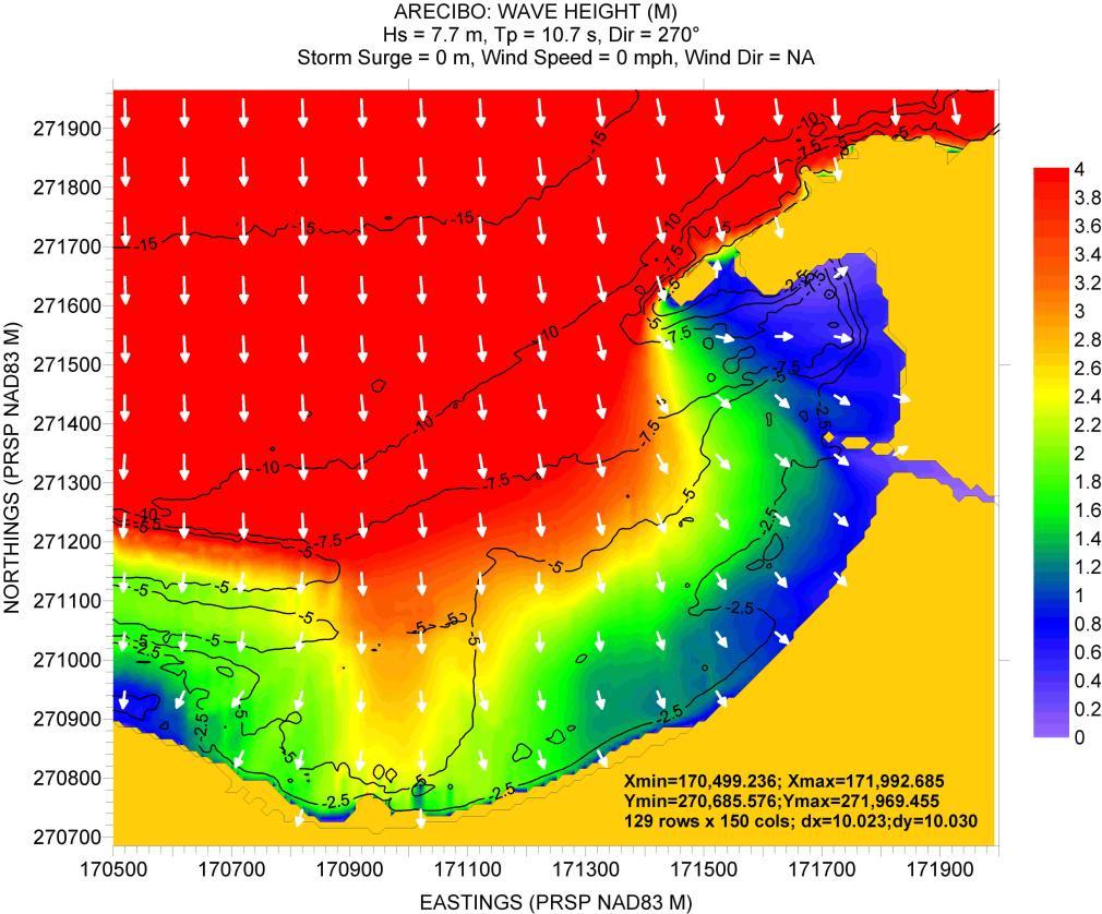
Figure 187. Hs contour plot for (nested) Charlotte Amalie, St. Thomas, based on the scenario listed along the top margin of figure. 119
Figure 188. Hs contour plot for Charlotte Amalie, St. Thomas, based on the scenario listed
along the top margin of figure.
Figure 189. Hs contour plot for (nested) Charlotte Amalie, St. Thomas, based on the scenario listed along the top margin of figure.
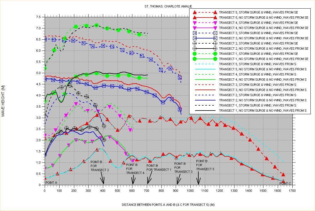
Figure 190. Significant wave height “slices” for Charlotte Amalie Bay, St. Thomas.
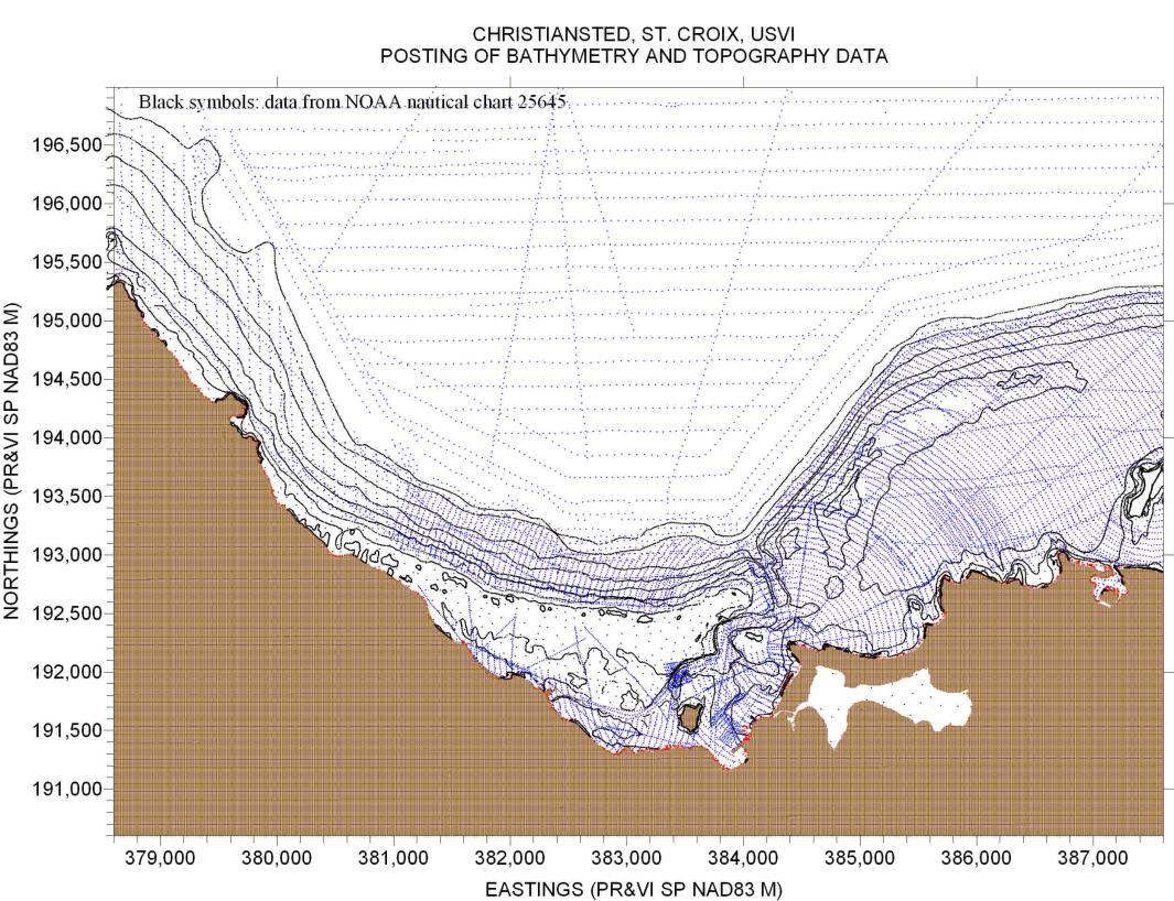
Figure 191. Posting showing location of bathymetry and topography values for Christiansted Bay, St. Croix.
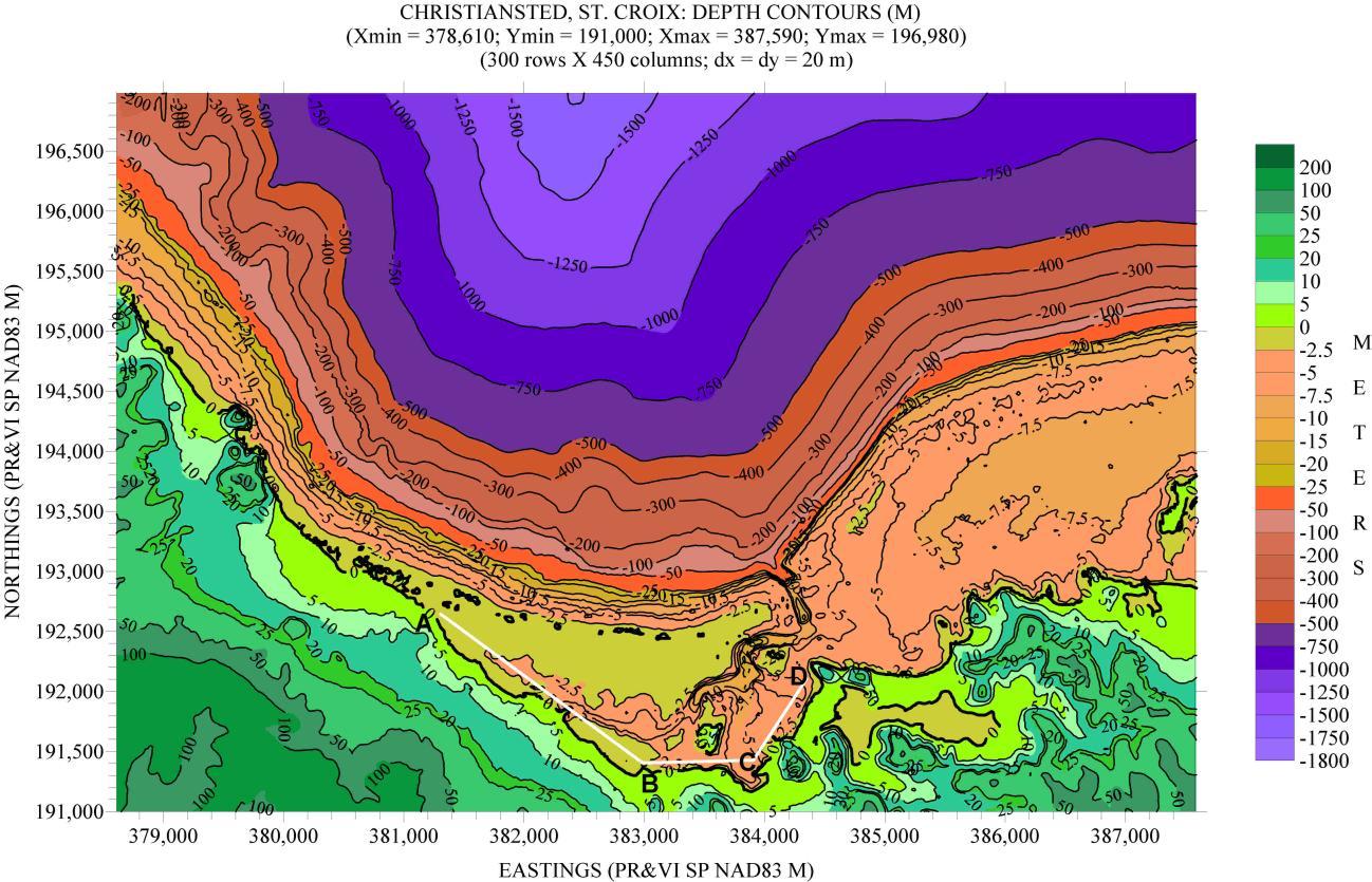
Figure 192. Depth contour plot of computational grid for Christiansted Bay, St. Croix.
Figure 193. Hs contour plot for Chrsitiansted, St. Croix, based on the scenario listed along the top margin of figure.
Figure 194. Hs contour plot for Chrsitiansted, St. Croix, based on the scenario listed along the top margin of figure.
Figure 195. Hs contour plot for Chrsitiansted, St. Croix, based on the scenario listed along the top margin of figure.
Figure 196. Hs contour plot for Chrsitiansted, St. Croix, based on the scenario listed along the top margin of figure.
Figure 197. Hs contour plot for Chrsitiansted, St. Croix, based on the scenario listed along the top margin of figure.
Figure 198. Hs contour plot for Chrsitiansted, St. Croix, based on the scenario listed along the top margin of figure. 125
Figure 199. Significant wave height “slices” for Christiansted Bay, St. Croix. 126
Figure 200. Posting showing location of bathymetry and topography values for Frederiksted Bay, St. Croix.
Figure 201. Depth contour plot of computational grid for Frederiksted Bay, St. Croix.
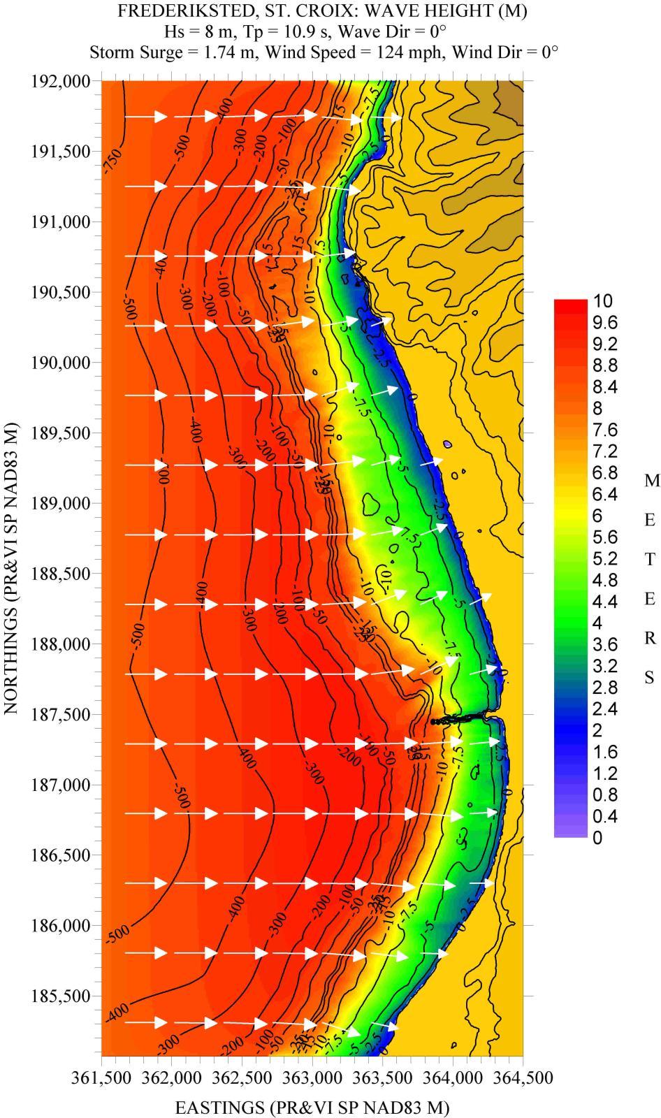
Figure 202. Hs contour plot for Frederiksted, St. Croix, based on the scenario listed along the top margin of figure.
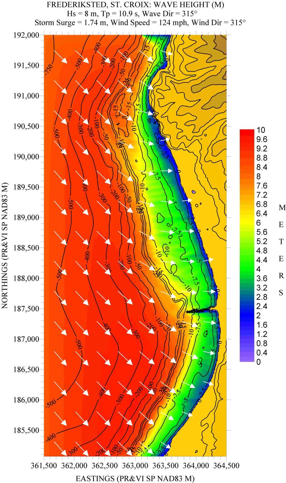
Figure 203. Hs contour plot for Frederiksted, St. Croix, based on the scenario listed along the top margin of figure.
Figure 204. Hs contour plot for Frederiksted, St. Croix, based on the scenario listed along the top margin of figure.
Figure 205. Hs contour plot for Frederiksted, St. Croix, based on the scenario listed along the top margin of figure.
Figure 206. Hs contour plot for Frederiksted, St. Croix, based on the scenario listed along the top margin of figure.
Figure 207. Hs contour plot for Frederiksted, St. Croix, based on the scenario listed along the top margin of figure.
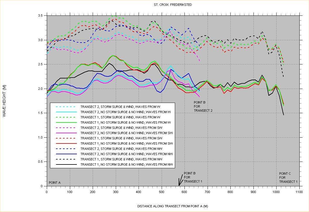
Figure 208. Significant wave height “slices” for Frederiksted, St. Croix.
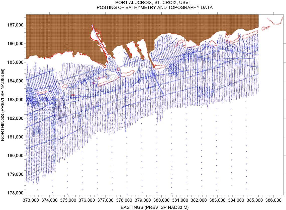
Figure 209. Posting showing location of bathymetry and topography values for Port Alucroix, St. Croix.
Figure 210. Depth contour plot of computational grid for Port Alucroix, St. Croix 138
Figure 211. Hs contour plot for Port Alucroix, St. Croix, based on the scenario listed along the top margin of figure.
Figure 212. Hs contour plot for Port Alucroix, St. Croix, based on the scenario listed along the top margin of figure.
Figure 213. Hs contour plot for Port Alucroix, St. Croix, based on the scenario listed along the top margin of figure.
Figure 214. Hs contour plot for Port Alucroix, St. Croix, based on the scenario listed along the top margin of figure.
Figure 215. Hs contour plot for Port Alucroix, St. Croix, based on the scenario listed along the top margin of figure.
Figure 216. Hs contour plot for Port Alucroix, St. Croix, based on the scenario listed along the top margin of figure.
Figure 217. Significant wave height “slices” for port Alucroix, St. Croix.
INTRODUCTION
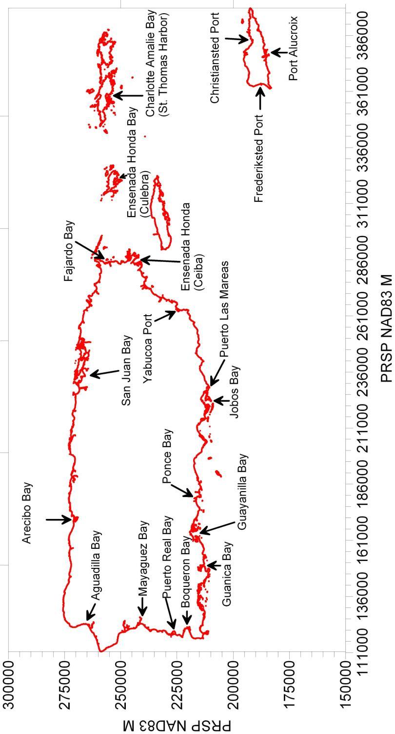
The geographic location of Puerto Rico and the U.S. Virgin Islands (USVI) makes them very vulnerable to being hit by hurricanes, as history has shown. And this includes Category 4 and 5 hurricanes. It is the purpose of this study to use a state-of-the-art wave transformation wind-wave model, together with recently-acquired, high-density, bathymetry to ascertain what can be expected in a worst-case scenario, for the main ports, harbors, and bays in Puerto Rico and the USVI. Figure 1 shows the location of the ports and bays studied.
METHODOLOGY
The physics of wind wave transformation over very complex bathymetry, and its interaction with port and harbor structures, is very complex. And it becomes even more complex and difficult when forced by hurricane winds, for which not much is known to this day. There is no numerical wave model capable, to this day, of accurately modeling all of the factors involved in the wave transformation process. Boussinesq wave models are one option, but they require enormous computer resources, and they still suffer from the lack of wind input (though the author knows of at least one very recent attempt to include wind input in Boussinesq wave models). The other option are the spectral models, like the SWAN model (http://fluidmechanics.tudelft.nl/swan/default.htm). But until the last version that came out this year, wave diffraction was not included. And diffraction could be a factor to consider in regions of significant and sudden changes in depth, like it could happen inside bays and harbors. Not to mention that diffraction is certainly important close to manmade structures.
With version 40.41 of the SWAN model an attempt has been made to include diffraction effects. Due to the fact that spectral models, by definition, do not include wave phase information (they are also called phase-averaging models, while the Boussinesq models are called phaseresolving models), the inclusion of physics which are explicitly dependent on phase information (like diffraction) has to be done in a very approximate way. The new version comes with a wave diffraction test case (the classic one of constant depth diffraction by a semi-infinite wedge), though no comparison is made with the known analytic and/or numerical solutions to this problem. In the bulletin board of the model it is acknowledged that the inclusion of diffraction is still in an experimental stage, and that much testing still remains to be done. It should be stated that the inclusion of diffraction is an option in the model, and that its best use requires more memory, and CPU, resources than its non-inclusion. This involves the use of a very finely discretized wave angular spectrum. In this study a compromise was made in that the highest angular resolution that could be accommodated with the available RAM memory in the PC used (4 GB) was used. The larger the computational domain, the smaller the resolution. But never a resolution smaller than 15° was used. For most of the computational grids, especially for the nested ones, we could afford an angular resolution of 3°. It is for this reason that a qualitative test was made in which a small computational grid (Puerto de Yabucoa) was utilized to make comparison runs with no diffraction, and diffraction with angular resolutions of 15°, 3°, and 0.5°. This is discussed before.
Since the objective is to estimate what could be expected under a worst-case scenario, the following approach was followed. For boundary conditions for the model (significant wave
1. Location of the ports and harbors evaluated in this study.
Figure
height, Hs, peak wave period, Tp) we used the results of a study (Hurricane Hazard Information for Caribbean Coastal Construction) sponsored by the Organization of American States (http://cdcm.methaz.org/cdcm/index.html/) in which Maximum Likelihood Estimates of Hs and Tp values are given all along the Caribbean basin, for different return periods. In our case we limited ourselves to the 100-year return period. The above study also gives the 100-year MLE for 10minute averaged winds, which were the values used when wind forcing was required. In all of the simulations where wind forcing was used it was assumed that it was constant in time, magnitude, direction, and in space. For the largest computational grids the constancy in direction and space is not a completely accurately scenario. Hurricane winds can be considered constant in direction and in space only for the smaller grids. The fact that hurricane winds follow curved trajectories tends to reduce the fetch. So in this sense, when using “constant” hurricane forcing for large computational grids we should be getting conservative results.
In the SWAN model the above values of Hs and Tp are fit to a Jonswap-type frequency spectrum, which is then used as deep-water boundary condition, and is assumed constant along a whole boundary (typically the deep water boundary), or a section of it. A cosm(- p) directional distribution function was assumed, in which p is the peak wave direction, which was assigned by the user based on what was thought was the deep-water peak wave directions that could result in the worst case scenario inside the location under study. The default value of m = 2 was assumed for all of the simulations, corresponding to a Directional Spreading (DSPR) of 31.5°. The Jonswap peak enhancement factor, (, was taken as 3.3.
The frequency spectrum was broken down into 19 frequency bins, going from a minimum wave period of 3 s, up to a maximum wave period of 20 s.
In this report we will proceed as follows. The next section presents a brief overview of the SWAN model. This is followed by a section describing the bathymetry used, followed by a discussion of a qualitative diffraction test. Then we will present the model results, in a case by case basis. Finally, we will present the conclusions.
The SWAN Model (Version 40.41)
The following is directly taken from the SWAN link given above (http://fluidmechanics.tudelft.nl/swan/default.htm) . For further details one should go to that link, and also read the Users Manual. An important factor, which are verification tests, can be found at the link titled References. It suffices to mention that the SWAN model is a well-tested model, being used worldwide.
Features of SWAN
Physics
SWAN accounts for the following physics:
• Wave propagation in time and space, shoaling, refraction due to current and depth, frequency shifting due to currents and non-stationary depth.
• Wave generation by wind.
• Three- and four-wave interactions.
• White-capping, bottom friction and depth-induced breaking.
• Wave-induced set-up.
• Propagation from laboratory up to global scales.
• Transmission through and reflection (specular, diffuse and scattered) against obstacles.
• Diffraction.
Some of the physics mentioned above are optional, so it should be stated that in our computer runs all of the above were included. The SWAN model that was run was the MS Windows version, with the inherent memory limitations that this implies.
BATHYMETRY AND TOPOGRAPHY
The bathymetry used for the preparation of the computational grids was a combination of the National Ocean Service (NOS) data listed on http://poseidon.uprm.edu, and recently (2001) acquired SHOALS data. In order to show the coverage density, for each location a posting of the input data is shown. This is very important since no matter how good the wave model is, the results are as reliable as the input data. For the south coast, between La Parguera and Bahía de Jobos no SHOALS data could be obtained by both the US Army Corps of Engineers and by the USGS. The reason is unknown. But for this same coast there exist relatively good coverage by NOS data. For the rest of the coast SHOALS is available, but in some areas, again, there is no coverage, in this case because of turbidity problems. You can see the areas of SHOALS coverage by the high density of points in the figures showing the posting of the points.
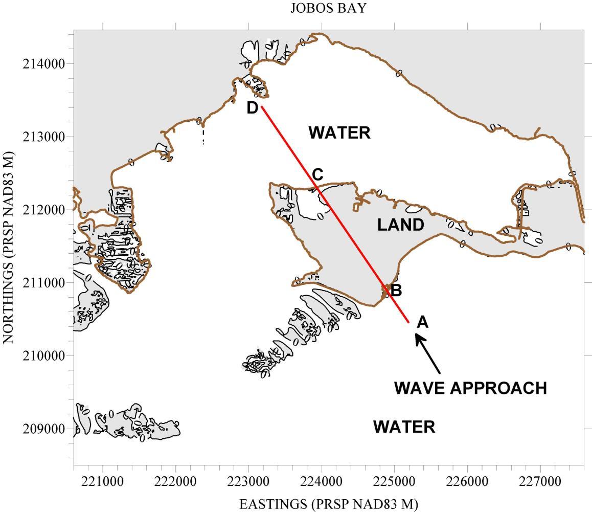
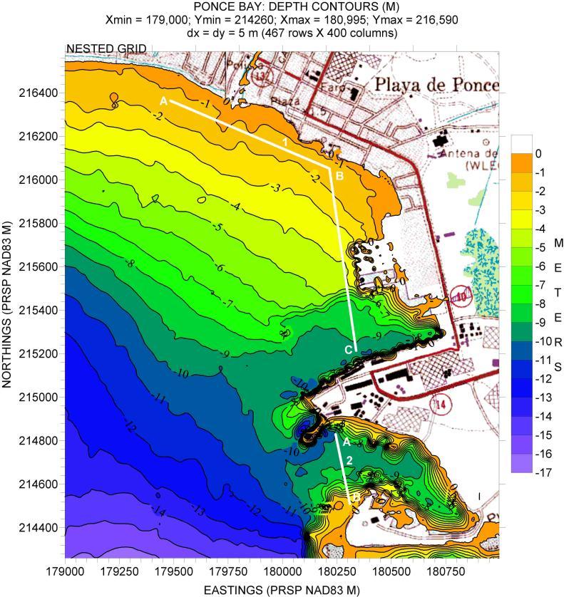
For the preparation of the computational grids, sub-aerial data (topography) was also used. But since some of the simulations involved adding the estimated 100-year return period storm surge elevations to all Mean Sea Level (MSL) water depths, this created some inland flooding over which the model could propagate waves. The topography used is the same, old and unreliable, Digital Elevation Model from the USGS available for Puerto Rico, with a cell size of 30 meters. Since the purpose of the study did not envision including wave propagation over flooded land, it was decided to, once the computational grid was prepared, set all land elevations (z values greater than 0) to a constant value of 10 m above MSL, above all storm surge elevations expected. This eliminates the possibility of wave propagation over flooded land. For open coastlines this does not make much of a difference, but in protected coastlines it could lead to an underestimation of the wave heights reaching the protected shoreline. The reason is very simple (see Figure 2). If the section of land between Points B and C in the figure is not flooded then the a wave train approaching Point A will be completely dissipated when it reaches the first land value at B. This implies that the wave height at Point D would be based (apart from waves reaching Point D from the left) on the effect of wind over the fetch CD, but starting with a wave height of zero meters at Point C. But if the piece of land between Points B and C is flooded then the wave height at Point C will be greater than zero, allowing for a greater wave height at Point D (if water depth allows it). So this is a caveat to have in mind when considering the wave heights inside protected shorelines.
Figure 2. Explanation of the possible effect of having all land values be 10 m high, as discussed in the report.
DIFFRACTION TEST
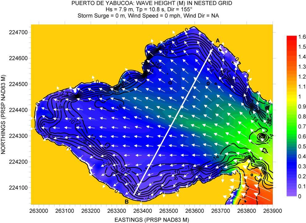
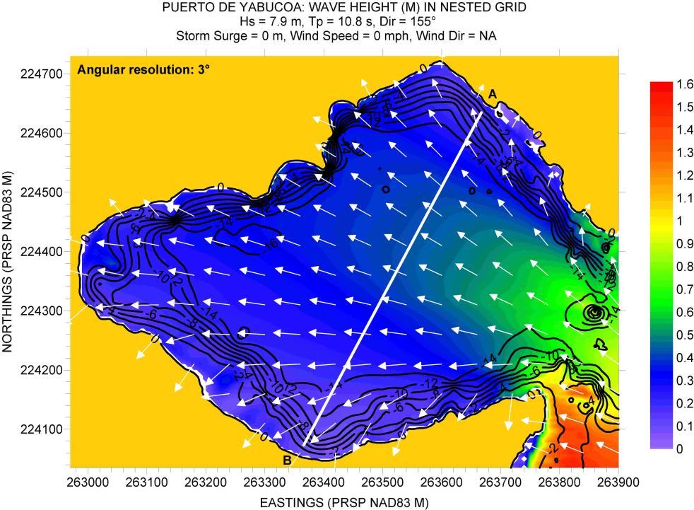
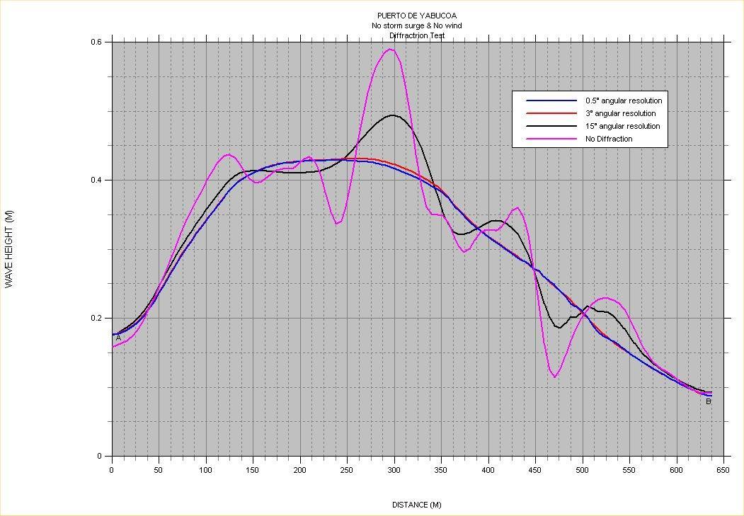
Since wave diffraction could be expected to play an important role in some of the locations studied, a qualitative test was made to see if it really made a difference. This was done at the Puerto de Yabucoa location, shown in Figure 3. Runs were made with no diffraction, and diffraction with angular resolutions of 15°, 3°, and 0.5°. By this is meant that the angular spectrum is broken down into bins of 15, 3, and 0.5 degrees in width. Figures 4, 5, 6 and 7 show the wave height field inside the port with the no diffraction, and diffraction with angular resolution of 15°, 3°, and 0.5°, respectively. The figures show the expected qualitative behavior. The no-diffraction case shows the typical narrow “beams” of energy expected for this case, while the other figures show how the energy concentrated in these “beams” is laterally diffused as diffraction effects are more accurately simulated. The figures show that there is not much difference between the results for angular resolution of 3° and 0.5°. Figure 8 shows a slice of the wave height field taken between Points A and B where this effect can be quantitatively seen.
Based on these results, the goal was to do all simulations with an angular resolution of 3°. But sometimes this became an impossibility due to memory limitations, in which case we were forced to reduce the angular resolution from 3° to 15°. This was a function of the computational grid size. All of the depth contour maps show grid information along the top margin, including
Figure 3. Location of diffraction test.
Figure 4. Wave height field for test with no diffraction.
Figure 5. Wave height field including wave diffraction. Angular resolution of 15°.
Figure 218. Wave height field including wave diffraction. Angular resolution of 3°..
7. Wave height field including wave diffraction. Angular resolution of 0.5°..
8. Comparison of results with no diffraction and diffraction with different angular resolution.
Figure
Figure
the size of the computational cells (dx and dy values).
RESULTS
For each location the model was run using as deep-water boundary conditions the 100-year MLE of Hs and Tp as obtained from the WEB page mentioned above. Two, and in some cases, up to three peak wave directions were modeled, obviously all having a component of propagation towards the location of interest. Each of the above runs was made twice, with and without wind forcing. The case of no wind forcing simulates the effect of a strong hurricane passing sufficiently far away from the location so that wind plays no role, and we just simulate the free propagation of the waves towards the location. The wind forcing, as mentioned above, was taken as the 100-year MLE for that location, and was assumed constant in space, direction, and time. In the simulations where wind forcing was included the 100-year storm surge was added to the MSL water depths. The simulations with no wind forcing were done with MSL water depths (no storm surge component) Although the WEB page from which the MLE of Hs, Tp, and wind also contained the 100-year MLE of the storm surge, the values used were the ones obtained by Mercado (1994). This was so because the Mercado results were obtained with a higher resolution, and more detailed, storm surge model than the model used to obtain the results listed in the WEB page.
We will start with San Juan Bay and move clockwise along the main island, followed by Culebra, St. Thomas, and then St. Croix. For those locations where a nested grid is used, results will be first presented for the outer grid, followed by the results inside the nested grid. The computations inside the nested grids are made using the output from the outer grids along the boundaries of the nested grid, as explained in the SWAN User’s Manual. This output consists of two-dimensional spectral information.
Results will be presented in two ways: 1) Filled contour plots of Hs on top of which deoth contour plots are overlaid, and 2) Hs values along selected “slices” (or transects) as shown in the figures. It should be mentioned that the depth contour plots overlaid on top of the Hs contour plots show the depth under MSL conditions, even for the simulations in which a storm surge has been added. Another thing to have in mind is that we are showing the results for the significant wave height, Hs, and that it should be understood that this implies the presence of higher waves capable of inflicting damage. And since we are interested in the very nearshore wave field, it should be understood that in very shallow waters the wave height is a function of water depth, irrespective of the wind speed. Since we have tried to show quantitative results by taking slices across Hs surfaces, and these slices are taken as close to shore as possible, then variations in Hs along the slice mainly reflect depth variations along the slice.
SAN JUAN BAY
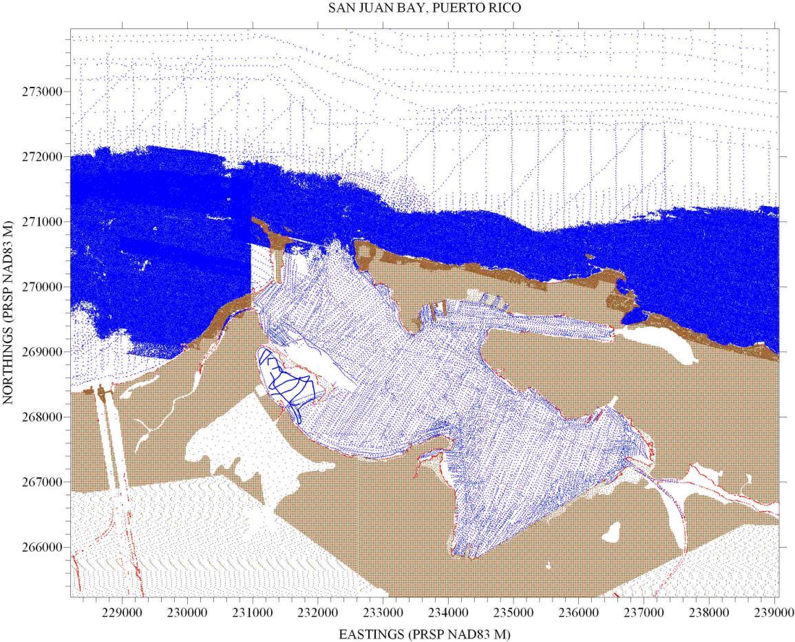
Figure 9 shows the locations where depth and land elevation values were available for preparing the San Juan Bay computational grid. It should be stated that the bathymetry used is from the early 1990’s and does not reflect changes due to dredging. The highly-packed blue values reflect the SHOALS data from 2001. The more sparse values to the north are the NOS values available in http://poseidon.uprm.edu. And this will be the same for all of the locations where SHOALS data is available.
Figure 9. Posting showing location of bathymetry and topography values for San Juan Bay.
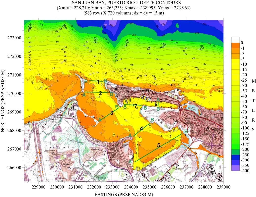
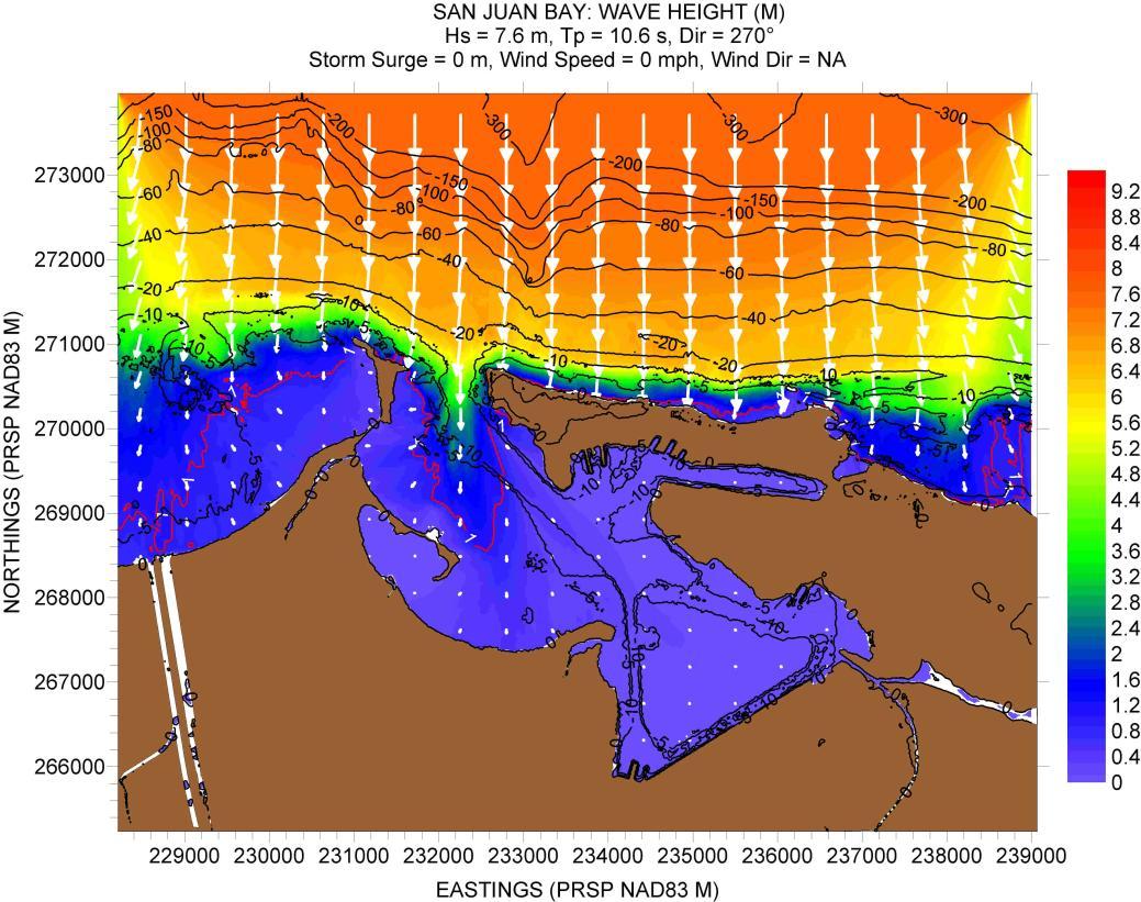
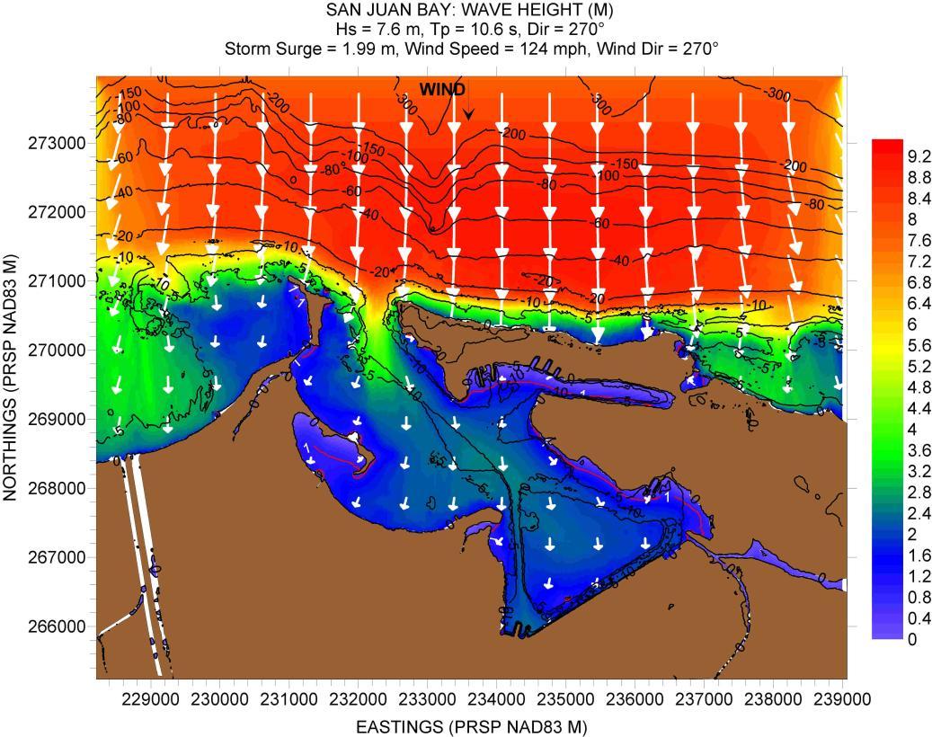
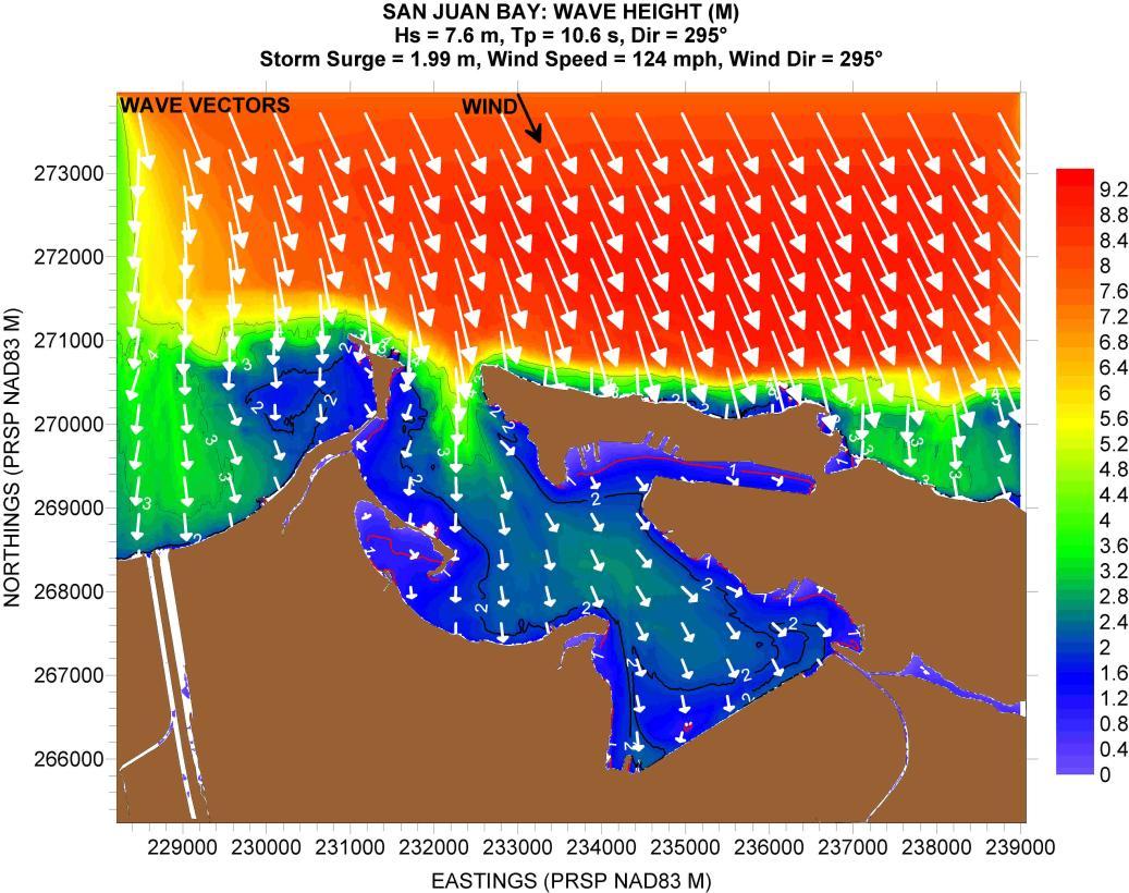
Figure 10 shows the depth contour map based on the computational grid used. Transects 1 to 7 are used to take a “slice” through the wave height field in order to help in quantifying how the waves entering through the bay entrance vary at different locations inside the bay. Figures 11 to 13 show contour plots of the Hs field inside the bay for the conditions indicated along the top of each figure. It remains to explain the convention used for wind and wave directions. The directions given along the top margin of the figures indicate the direction towards which the wind blows and waves propagate to. And 0° points towards the East, increasing in a counterclockwise direction. Also, not all figures are drawn with the same color scale for the right-hand-side colorbar.
Figure 10. Depth contour plot of the computational grid, and locations where Hs “slices” are going to be taken.
11. Hs contour plot for San Juan Bay based on the scenario listed along the top margin of figure.
Figure
Figure 12. Hs contour plot for San Juan Bay based on the scenario listed along the top margin of figure.
Figure 13. Hs contour plot for San Juan Bay based on the scenario listed along the top margin of figure.
The results show that the entrance to San Juan Bay serves as a choke point protecting the interior of the bay from larger waves propagating from offshore. This is quantitatively shown in Figures 14 and 15. With no wind forcing, waves in the interior of the bay rapidly decrease to 1 m, or less, in height. With wind forcing with a component along the longer axis of the bay, waves can reach 2 m along the southernmost part (Puerto Nuevo Docks). This corroborates what was observed during Hurricane Hugo in 1989, when those docks experienced structural damage due to waves. For Transects 6 (San Antonio Channel) and 7, with the wind direction assumed, the figures reflect the effect of wave growth with wind fetch, with the fetch starting along the south coast of the Isleta de San Juan.
Figure 14. Hs variation along the “slices” shown in the legend.
Figure 15. Hs variation along the “slices” shown in the legend.
FAJARDO
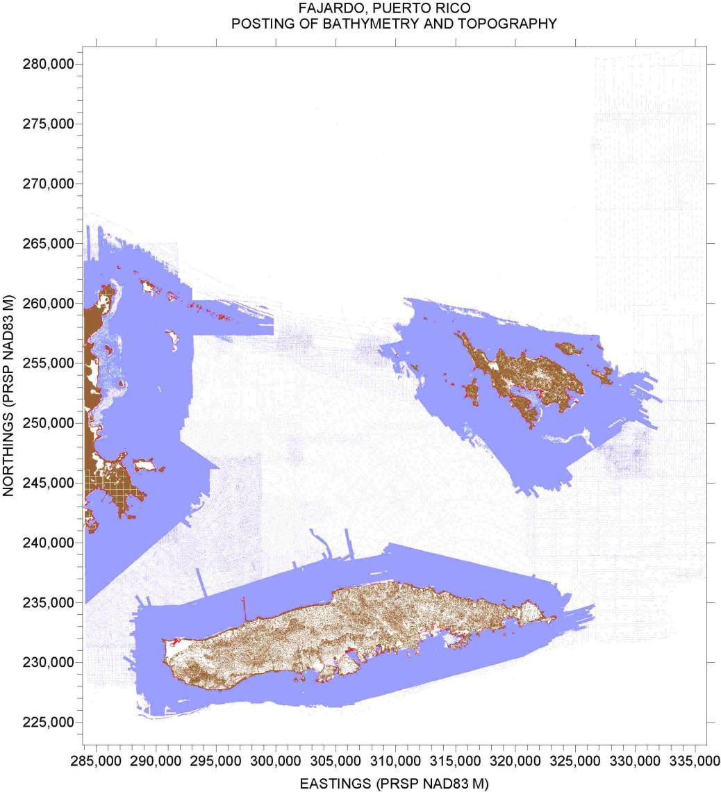
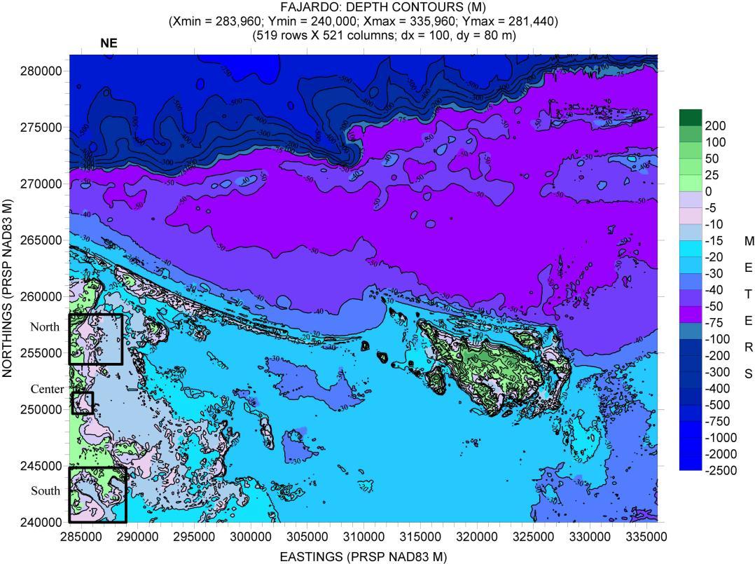
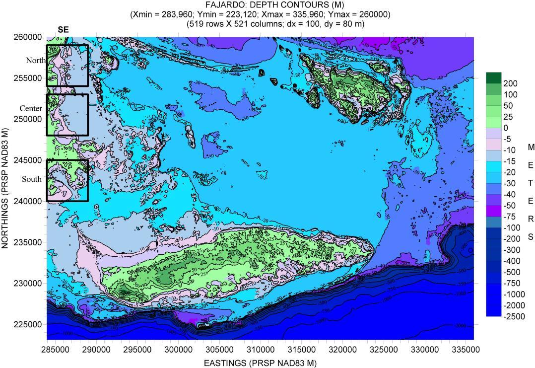
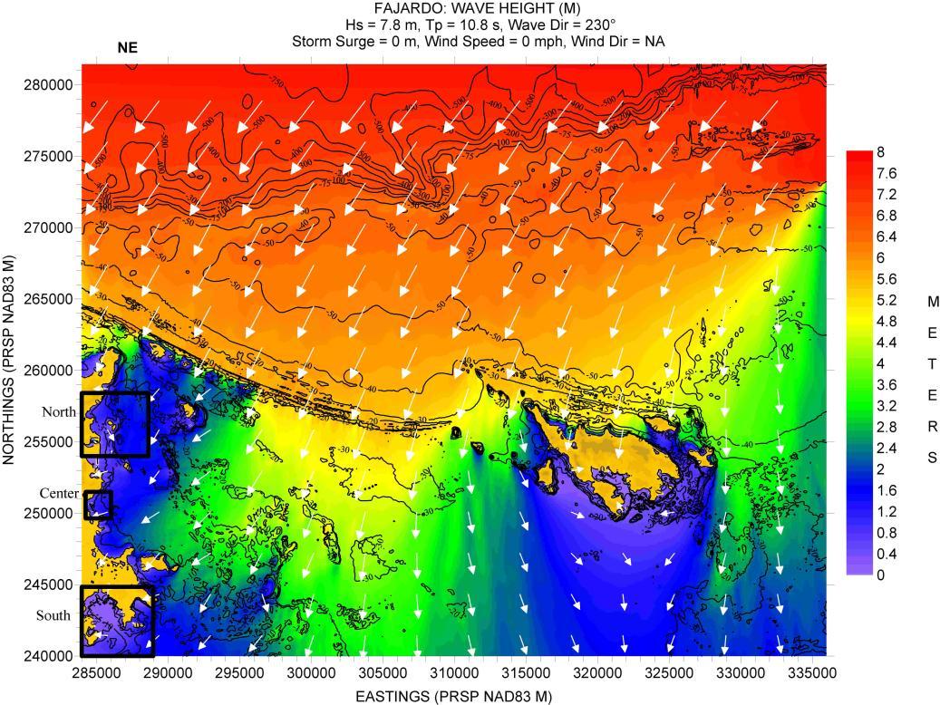
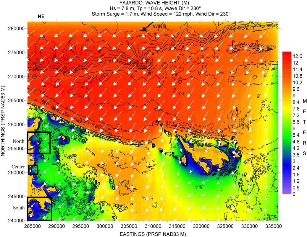
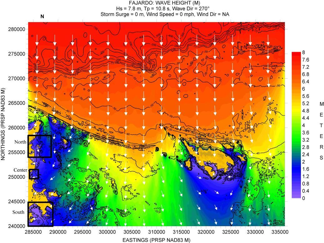
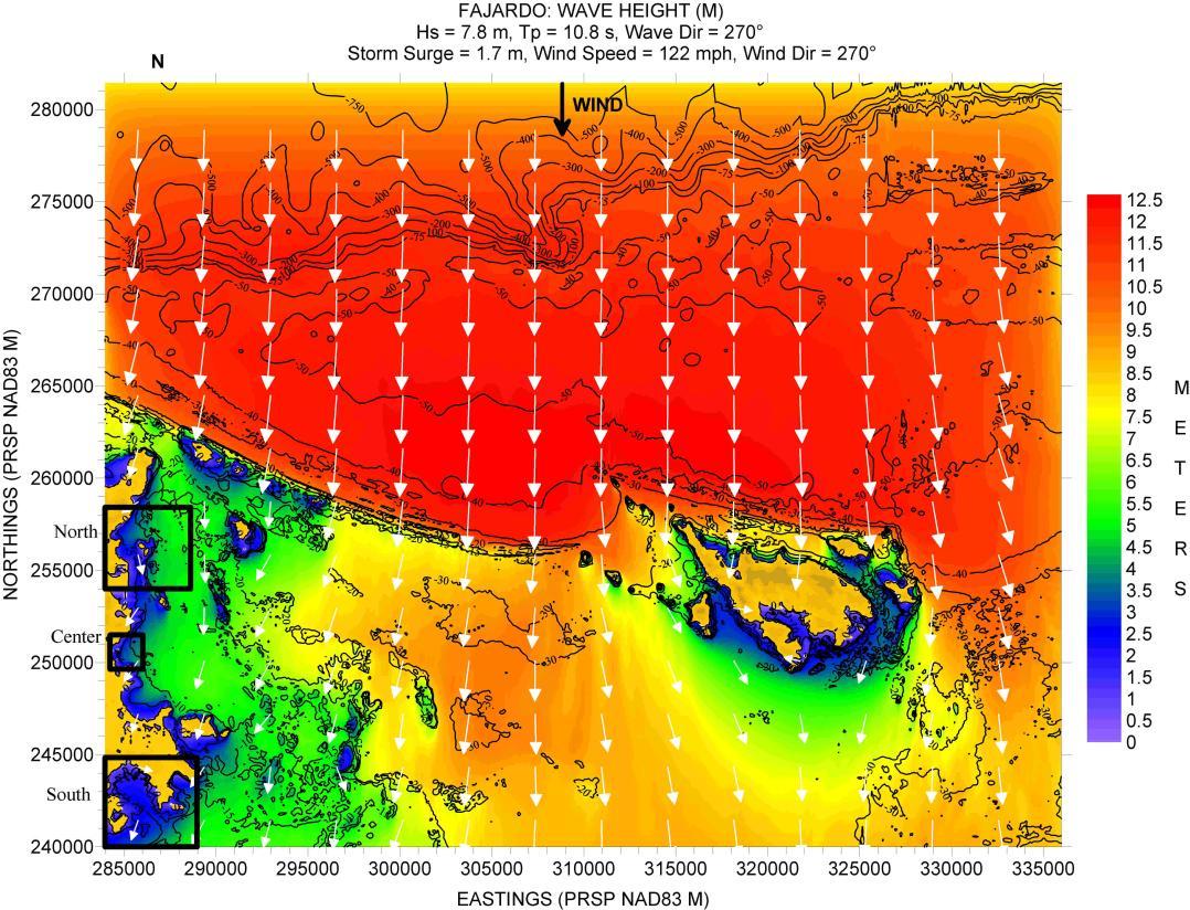
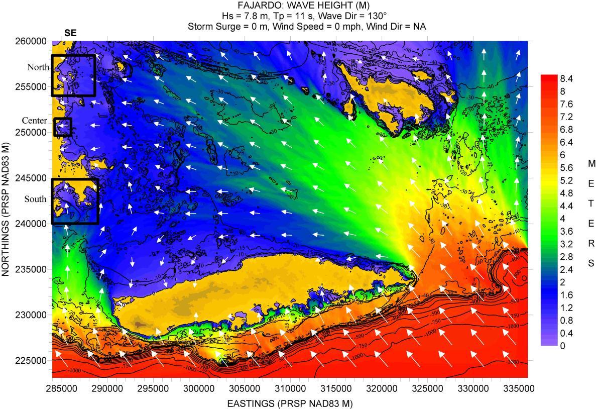
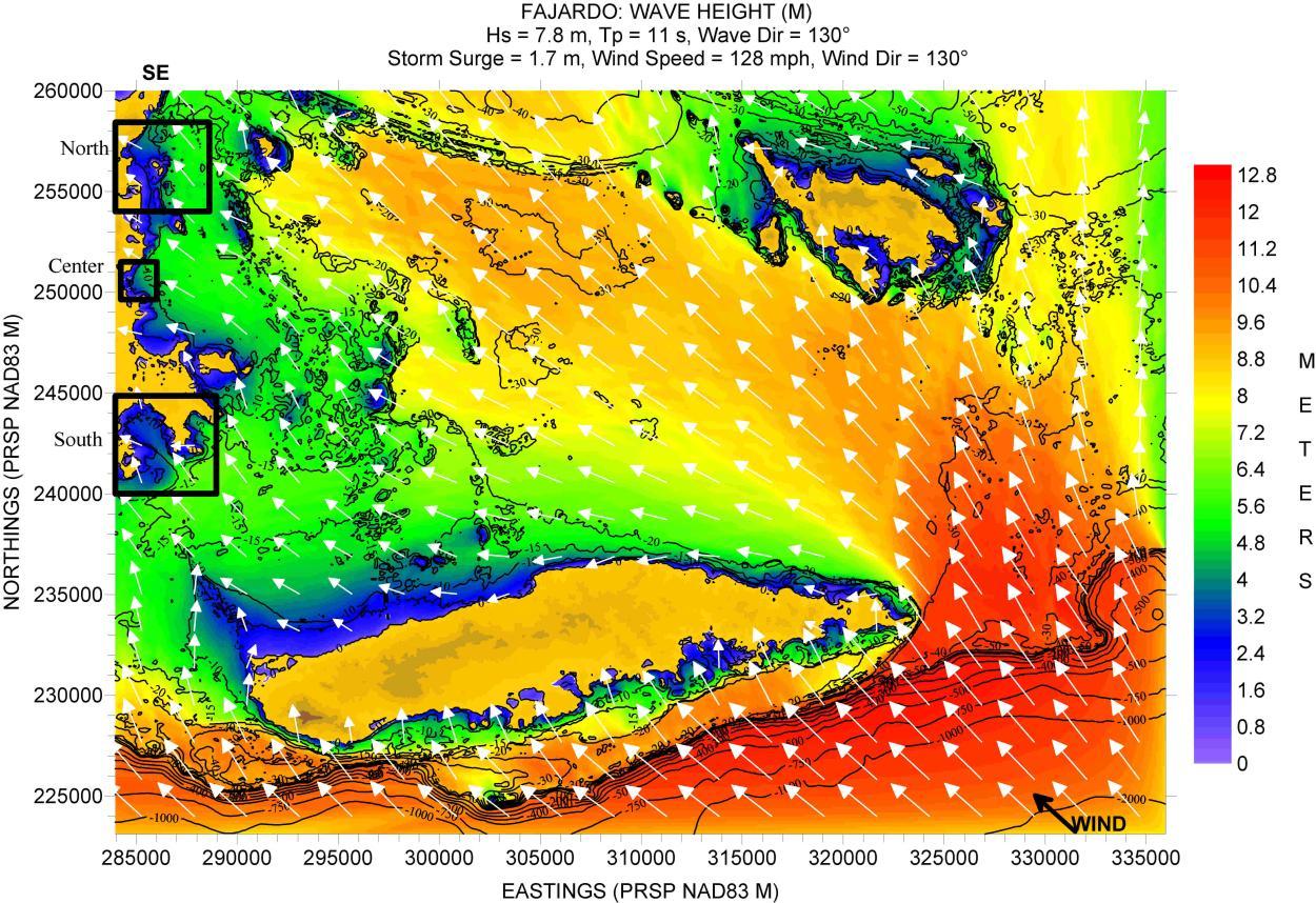
Figure 16 shows the locations where depth and land elevation values were available for preparing the “Fajardo” computational grid. The three locations of interest are shown in Figure 17 (the three nested grids). The east coast of the island is fronted by a very wide shelf (compared with the ones along the rest of the coasts), forcing the use of nested grids inside a large computational outer grid. Figures 17 shows the depth contour plot made from the data shown in Figure 16. For the east coast it was desired to evaluate waves propagating in from the northeast, north, and southeast (the south direction was considered only for the Ceiba-Ensenada Honda-Roosevelt Roads bays, and was done on a separate set of runs that follow). Because of its large extension, it was necessary to break the computational grid shown in Figure 17 into two smaller grids, as shown in Figures 18 and 19, and named “Fajardo NE” and “Fajardo SE”, respectively. The grid of Figure 18 was used for waves propagating from the northeast and north, while the grid of Figure 19 was used for the case of waves propagating in from the southeast.
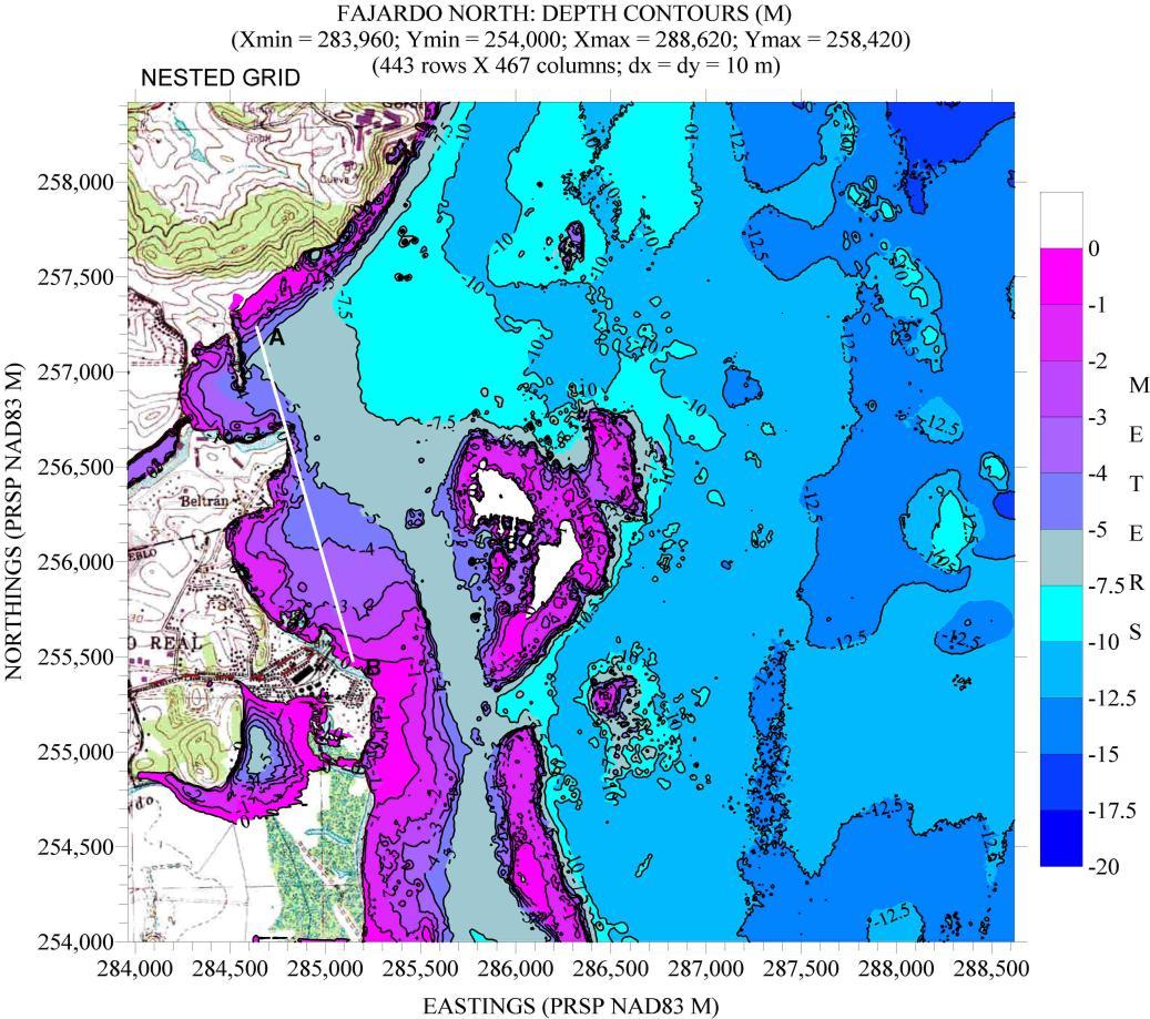
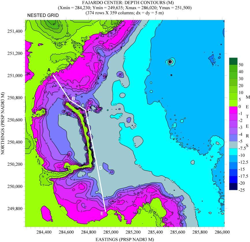
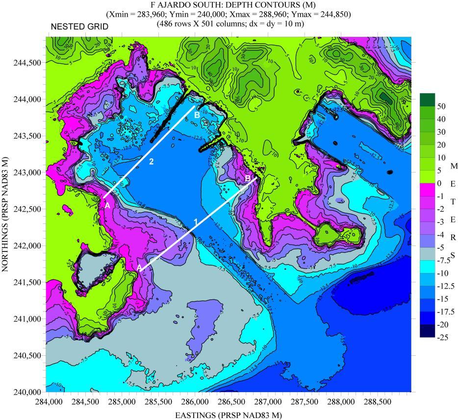
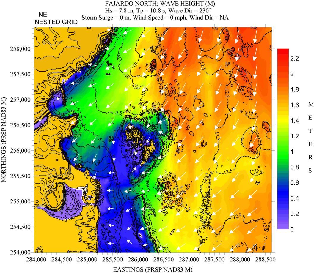
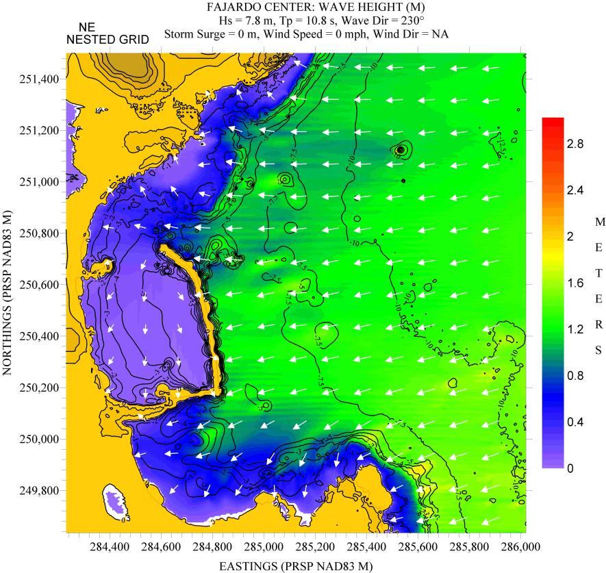
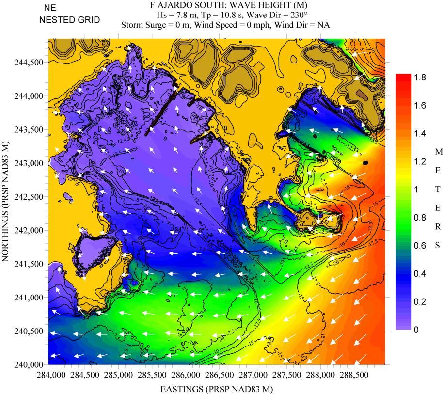
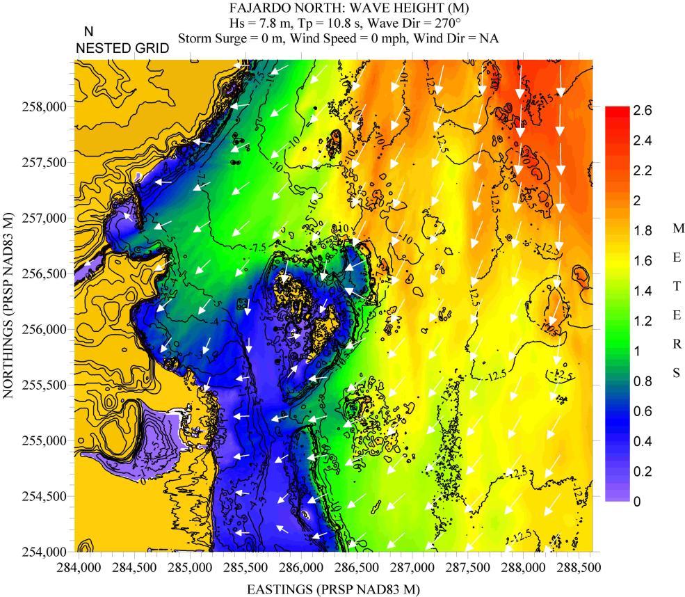
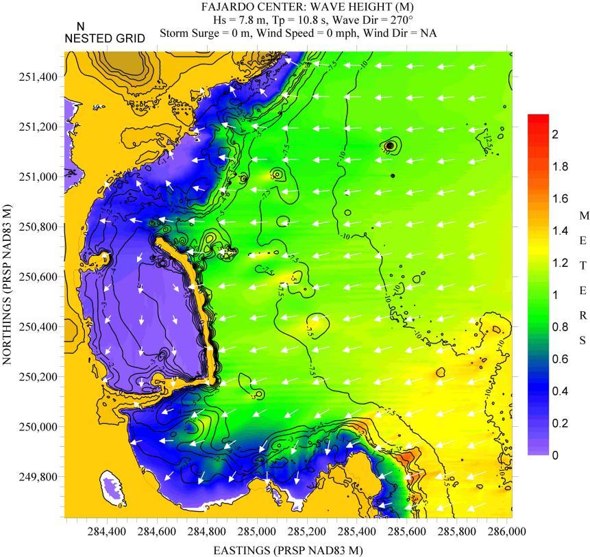
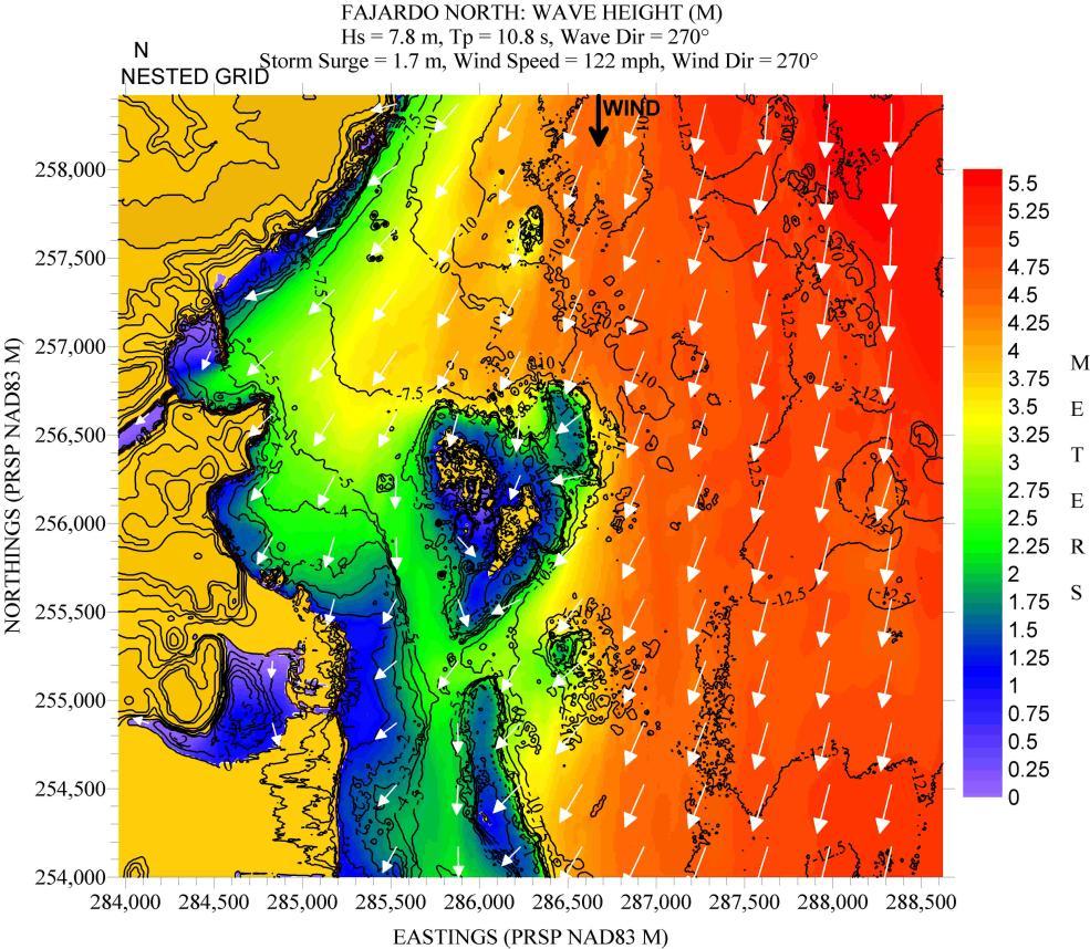
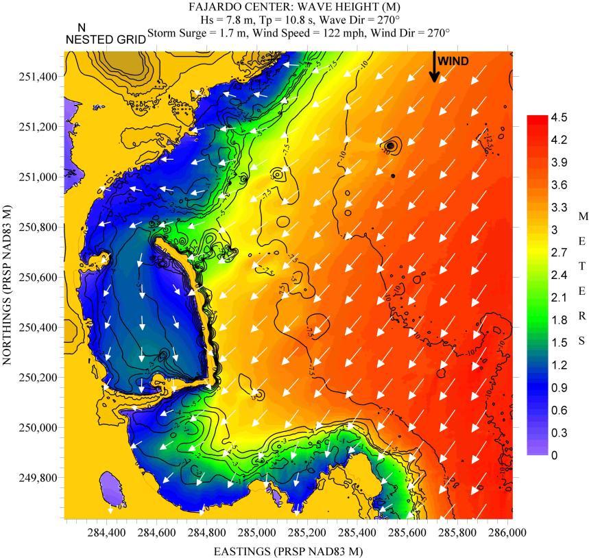
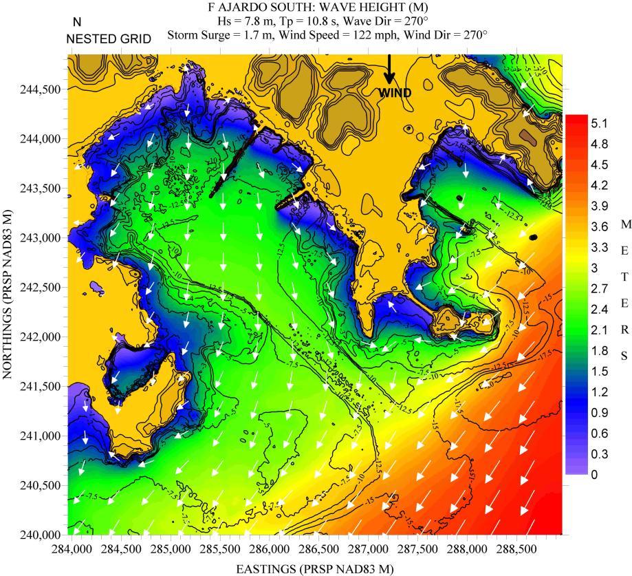
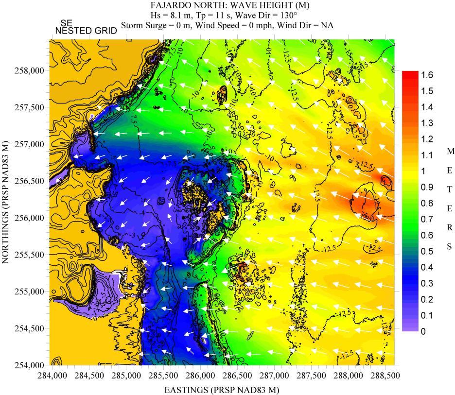
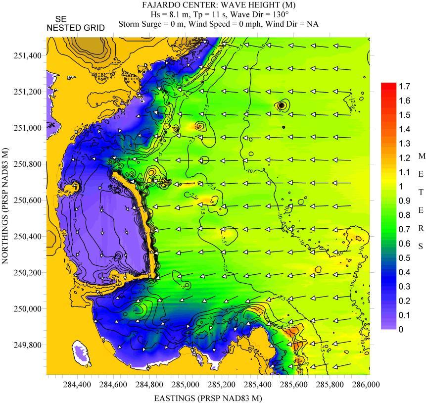
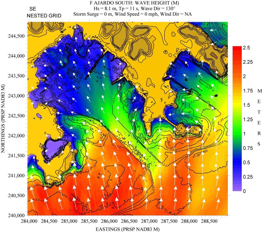
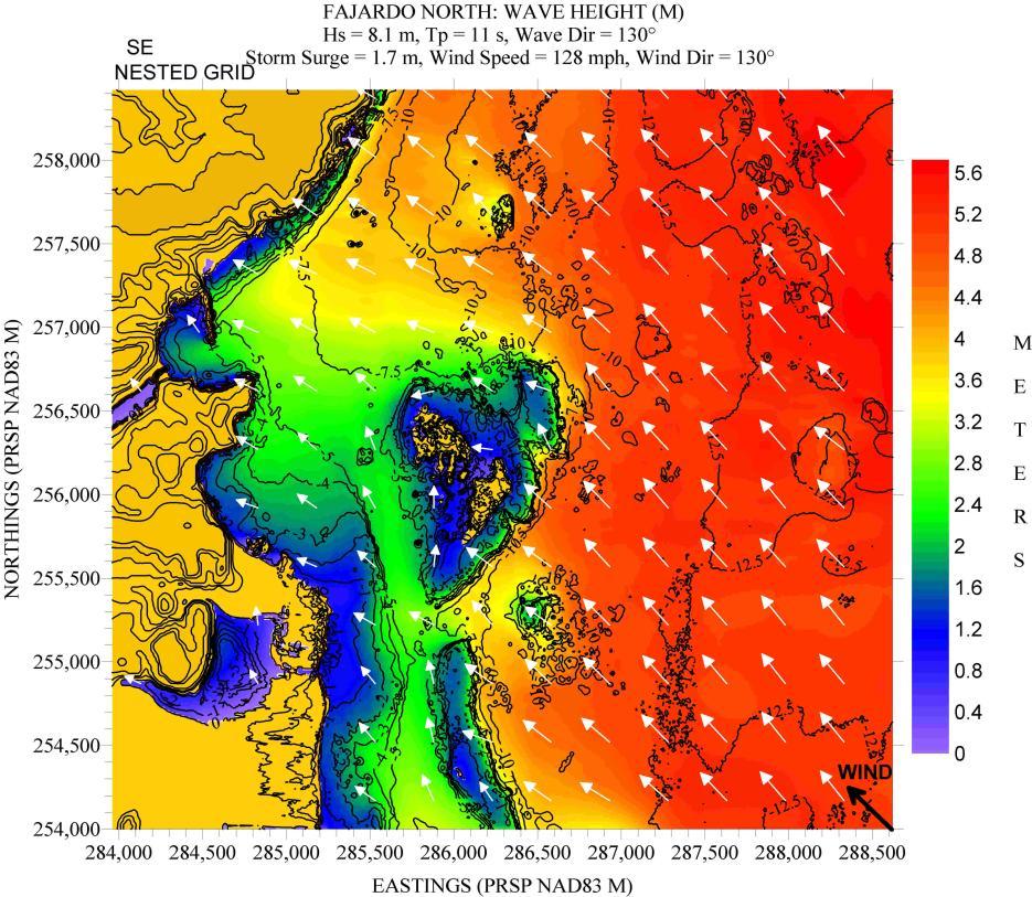
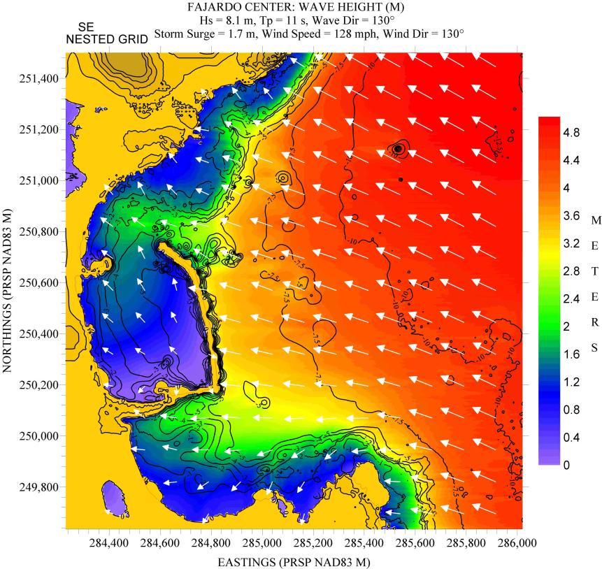
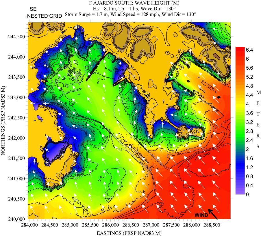
The nested grids are named as Fajardo North (covering approximately from Playa Sardinera south to Punta Barrancas; all of the area is known as Bahía de Fajardo; see Figure 20), Fajardo Center (covering Bahía Demajagua – where the Puerto del Rey Marina is located; see Figure 21), and Fajardo South (covering Ensenada Honda – also known as Roosevelt Roads – and Bahía de Puerca; see Figure 22). The figures show the location where “slices” of the wave height field will be taken.
FAJARDO NE
The results for “Fajardo NE” (see Figures 23 to 38) show the important role that the chain of small islands (known as La Cordillera) between Punta Las Cabezas de San Juan (Fajardo) and the island municipality of Culebra play in absorbing and scattering wave energy coming from the northeast and north. But this protection is weaker along the western section of the island chain, allowing some heavy surf to reach all the way south to “Fajardo Center”. As expected, the combination of storm surge plus wind forcing brings the worst scenarios.
FAJARDO SE
The results for “Fajardo SE” (see Figures 39 to 46) show the protection afforded by Vieques Island, with the possible exception of the “Fajardo North” basin, to the “Fajardo Center” and “Fajardo South” basins. The waves reaching the nested grids are mostly wind-generated along the fetch starting along the north coast of Vieques.
Let us now look at each nested grid individually.
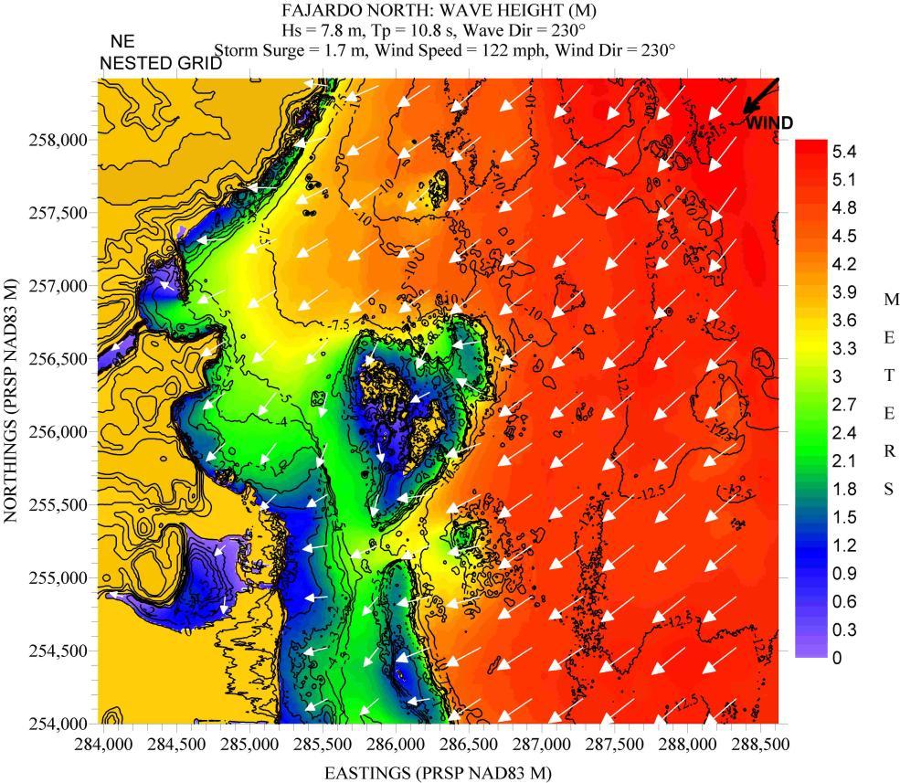
Fajardo North:
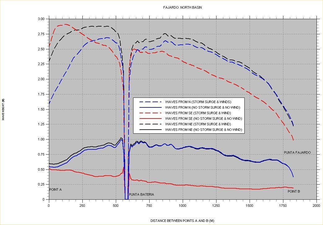
Figure 47 (slice for Fajardo North) shows that, while well protected for the case of no storm surge and no wind, the inclusion of both of these factors leads to significant wave heights of more than 2.5 m close to shore for all of the wave directions considered.
16. Posting showing location of bathymetry and topography values for the location named “Fajardo”.
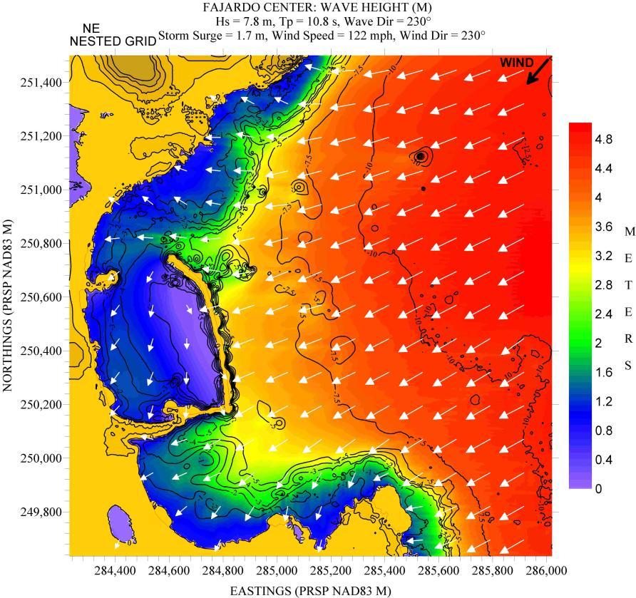
Fajardo Center:
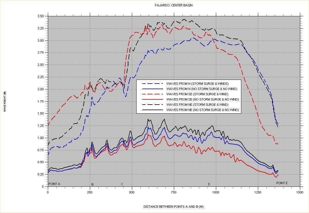
Figure 48 (slice for Fajardo Center) shows the same result, with Hs values above 3 m reaching the exposed side of the breakwater protecting the Puerto del Rey Marina under wind and storm surge conditions. The best protection is for waves from north.
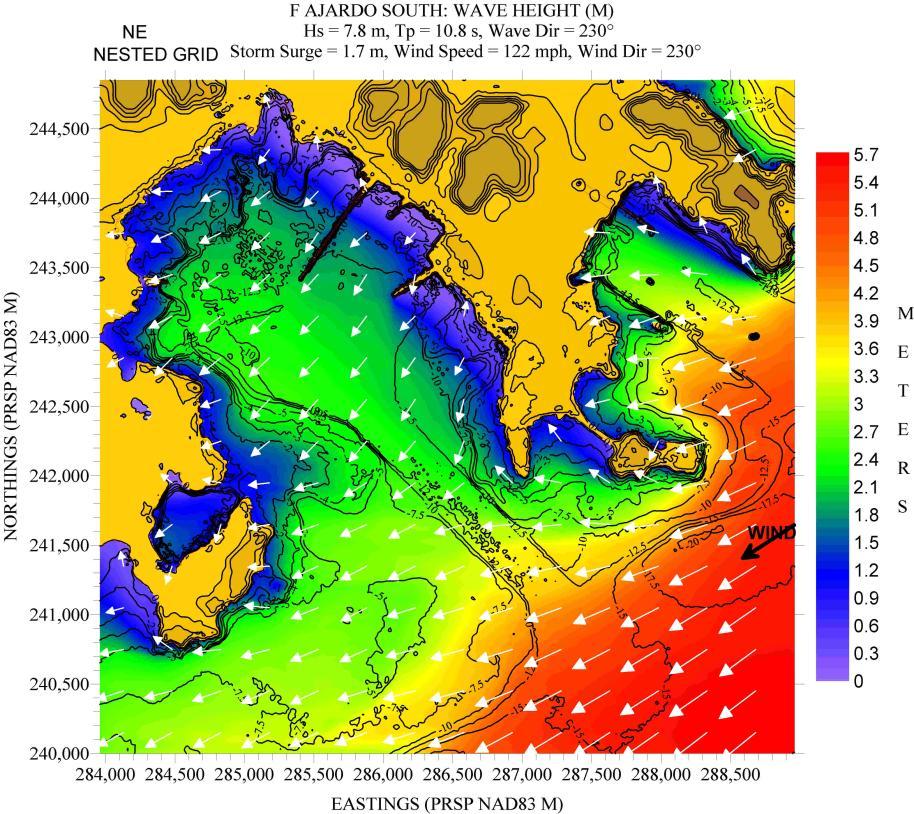
Fajardo South:
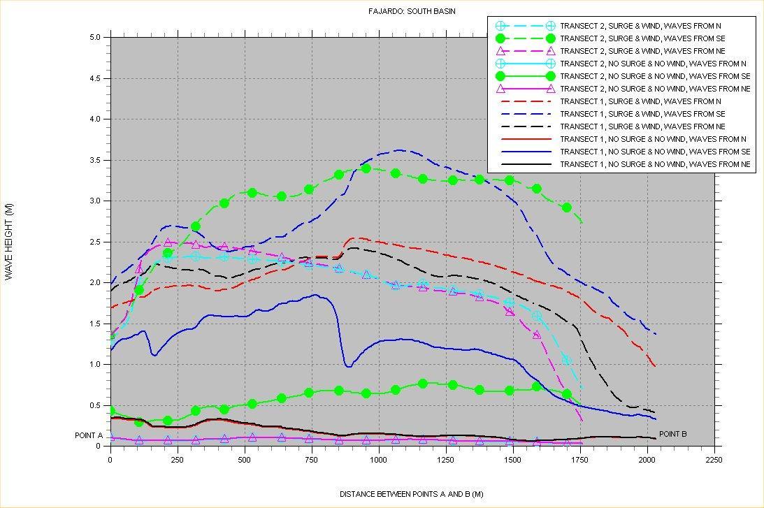
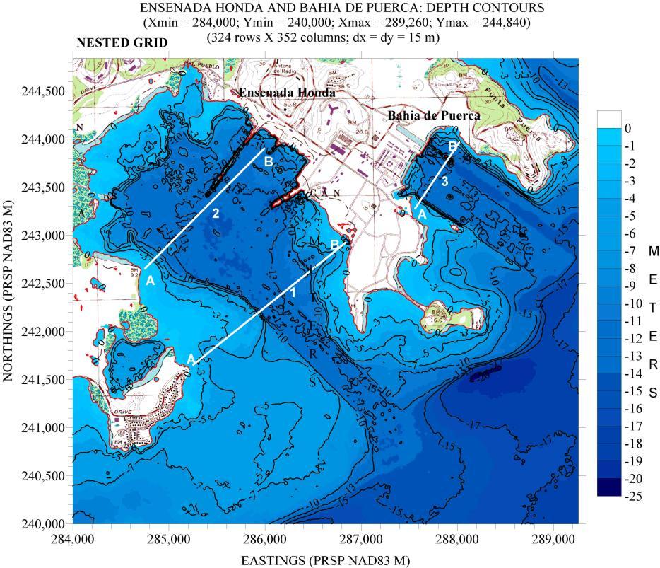
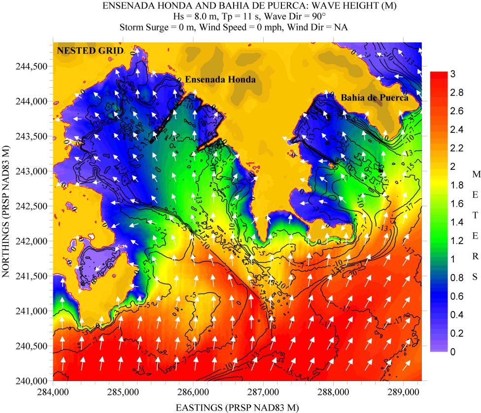
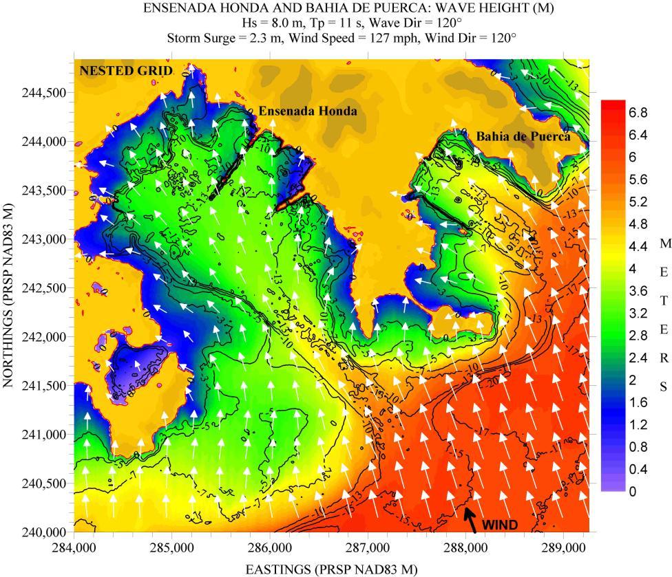
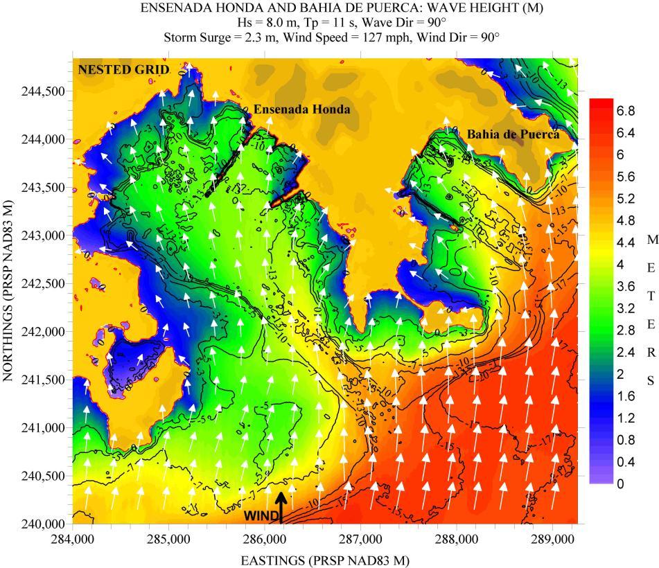
Figure 49 (slices for Fajardo South, inside Ensenada Honda – Roosevelt Roads) shows large waves (≥ 2 m) forming deep inside the bay (Transect 2) under wind and storm surge conditions irrespective of the direction of the wind and offshore waves. The wave directions inside the bay under wind forcing seem to show that the large waves are locally generated, that is, are formed inside the bay by the strong wind forcing. As expected, it is for waves and wind from the southeast
Figure
that conditions are the worst. In this case Hs values can be larger than 3 m along Transect 2 located along the middle of the bay.
17. Depth contour plot of original “Fajardo” computational grid.
Figure 18. Depth contour plot of the outer computational grid named “Fajardo NE”. Waves from the northeast and north are to be considered for this grid.
Figure
19. Depth contour plot of the outer computational grid named “Fajardo SE”. Only waves from the southeast are to be considered for this grid.
Figure
Figure 20. Depth contour plot for Fajardo North nested computational grid.
Figure 21. Depth contour plot for Fajardo Central nested computational grid.
Figure 22. Depth contour plot for Fajardo South nested computational grid.
23. Hs contour plot for
based on the scenario listed along the top margin of figure.
plot for
based on the scenario listed along the top margin of figure.
Figure
Fajardo NE
Figure 24. Hs contour
nested Fajardo North
margin of figure.
Figure 25. Hs contour plot for nested Fajardo Center based on the scenario listed along the top
Figure 26. Hs contour plot for nested Fajardo South based on the scenario listed along the top margin of figure.
margin of figure.
Figure 27. Hs contour plot for Fajardo NE based on the scenario listed along the top
Figure 28. Hs contour plot for nested Fajardo North based on the scenario listed along the top margin of figure.
Figure 29. Hs contour plot for nested Fajardo Center based on the scenario listed along the top margin of figure.
Figure 30. Hs contour plot for nested Fajardo South based on the scenario listed along the top margin of figure.
31. Hs contour plot for
based on the scenario listed along the top margin of figure.
listed along the top margin of figure.
Figure
Fajardo NE
Figure 32. Hs contour plot for nested Fajardo North based on the scenario
listed along the top margin of figure.
margin of figure.
Figure 33. Hs contour plot for nested Fajardo Center based on the scenario
Figure 34. Hs contour plot for nested Fajardo South based on the scenario listed along the top
margin of figure.
Figure 35. Hs contour plot for Fajardo NE based on the scenario listed along the top
Figure 36. Hs contour plot for nested Fajardo North based on the scenario listed along the top margin of figure.
the top margin of figure.
Figure 37. Hs contour plot for nested Fajardo Center based on the scenario listed along
Figure 38. Hs contour plot for nested Fajardo South based on the scenario listed along the top margin of figure.
39. Hs contour plot for
based on the scenario listed along the top margin of figure.
for
based on the scenario listed along the top margin of figure.
Figure
Fajardo SE
Figure 40. Hs contour plot
nested Fajardo North
plot for
based on the scenario listed along the top margin of figure.
listed along the top margin of figure.
Figure 41. Hs contour
nested Fajardo Center
Figure 42. Hs contour plot for nested Fajardo South based on the scenario
margin of figure.
Figure 43. Hs contour plot for Fajardo SE based on the scenario listed along the top
Figure 44. Hs contour plot for nested Fajardo North based on the scenario listed along the top margin of figure.
plot for nested
based on the scenario listed along the top margin of figure.
for
based on the scenario listed along the top margin of figure.
Figure 45. Hs contour
Fajardo Center
Figure 46. Hs contour plot
nested Fajardo South
Figure 47. Significant wave height “slices” for Fajardo North. Dip in curves occurs when the “slice” goes inland at Punta Batería.
Figure 48. Significant wave height “slices” for Fajardo Center.
Figure 49. Significant wave height “slices” for Fajardo South.
ENSENADA HONDA, CEIBA
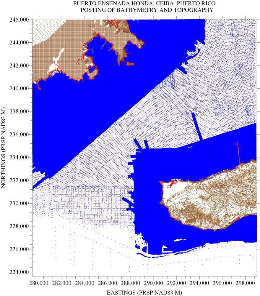
Figure 50 shows the locations where depth and land elevation values were available for preparing the Ensenada Honda, Ceiba (previously known as the Roosevelt Roads Navy Base) computational grid.
Figure 50. Posting showing location of bathymetry and topography values for Ensenada Honda, Ceiba.
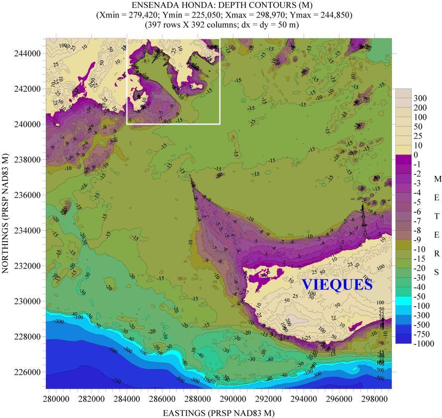
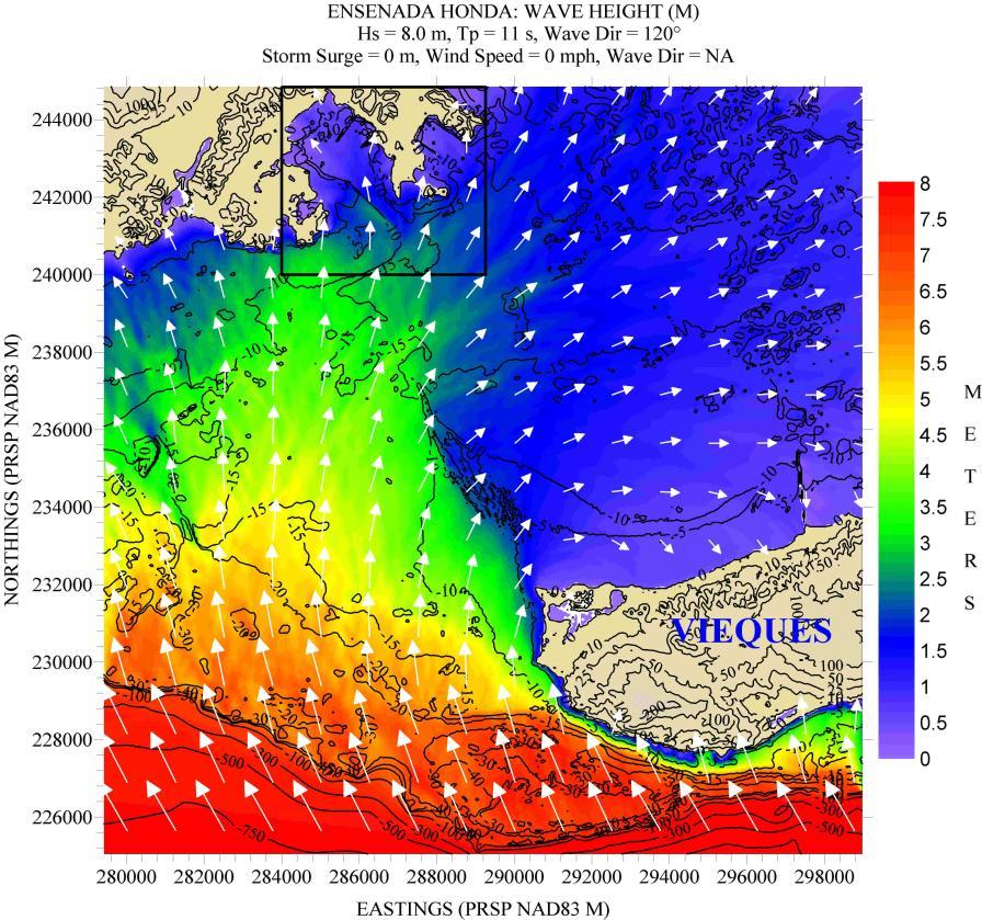
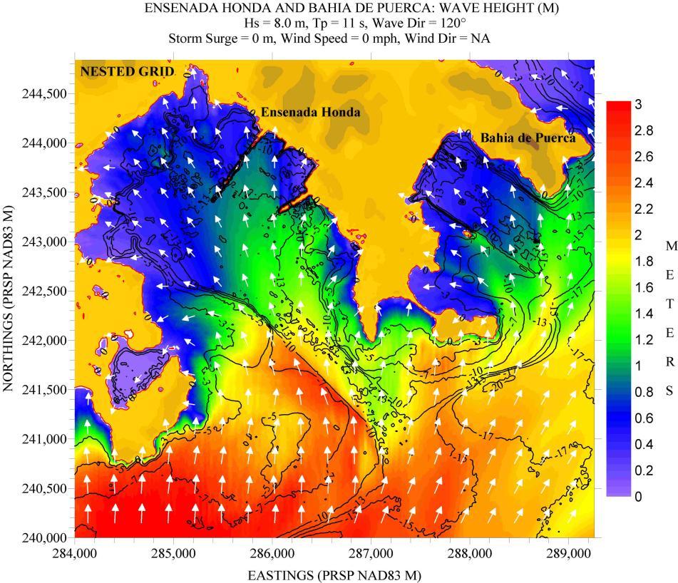
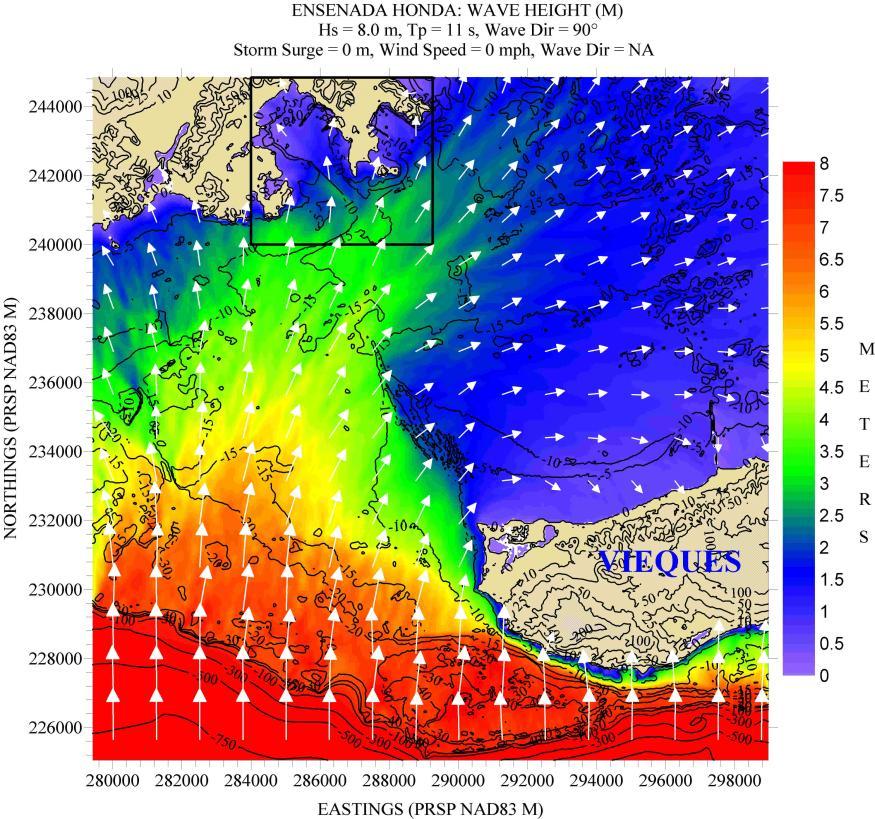
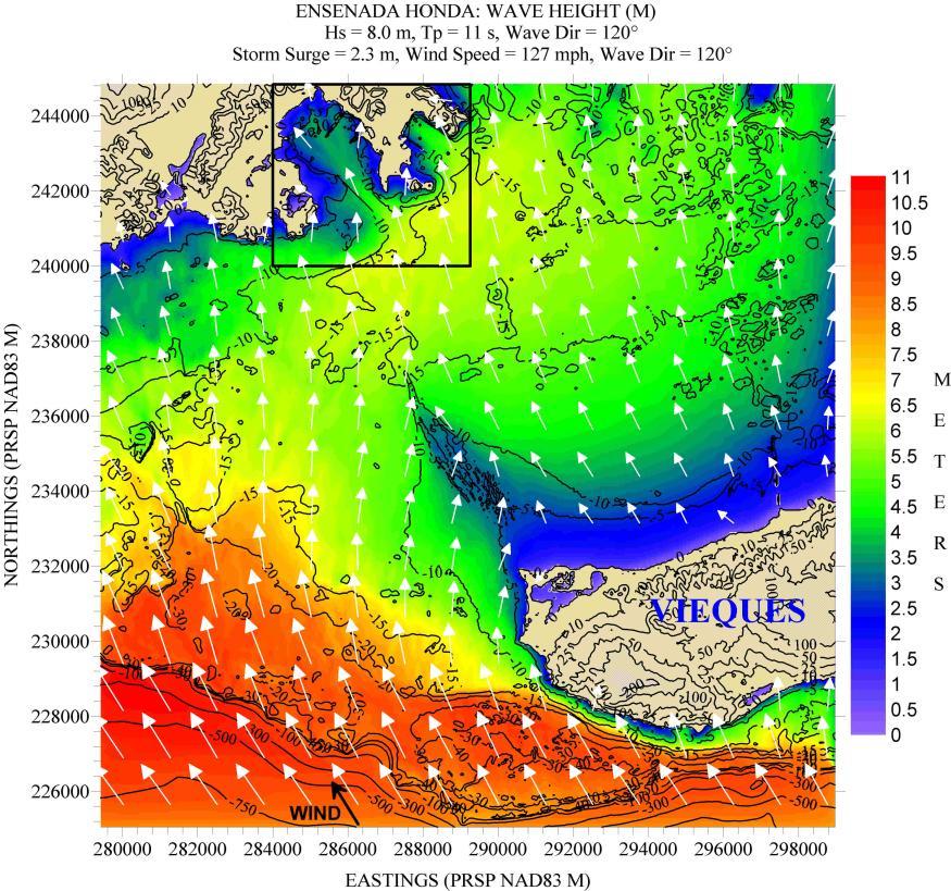
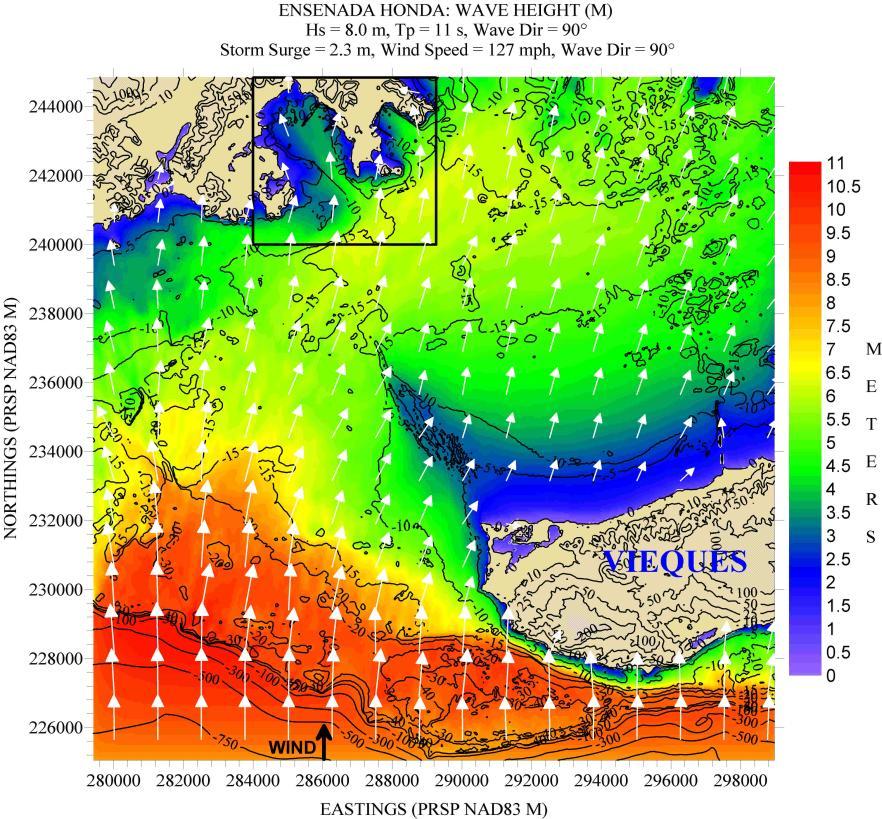
Figure 51 shows the depth contour plot for the outer computational grid for this location, and an outline of the nested grid to be used. Figure 52 shows the computational grid for the nested grid centered on Ensenada Honda Bay and Bahía de Puerca. The figure also shows the location of the three “slices” to be taken to quantify the wave heights. For this location waves and wind from the southeast and south will be used.
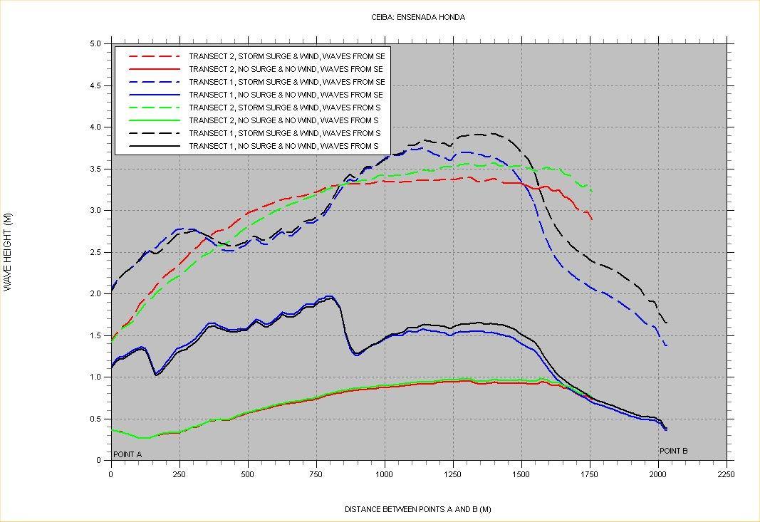
Figures 53 to 60 show the Hs field for the cases outlined along the top margin of each figure. This location is a good example showing the role that entrance channels play in allowing higher waves to enter into the bays and ports. Figure 61 shows the Hs variation along the slices inside Ensenada Honda Bay. It is not surprising that with such a wide entrance, when hurricane winds blow with a component along the axis of the entrance channel, large waves ( 2.5 m) can
Figure 51. Depth contour plot of the outer computational grid for Ensenada Honda, Ceiba.
Figure 52. Depth contour plot of nested computational grid for Ensenada Honda, Ceiba, and locations where “slices” are to be taken.
Figure 53. Hs contour plot for Ensenada Honda, Ceiba, based on the scenario listed along the top margin of figure.
Figure 54. Hs contour plot for (nested) Ensenada Honda, Ceiba, based on the scenario listed along the top margin of figure.
Figure 55. Hs contour plot for Ensenada Honda, Ceiba, based on the scenario listed along the top margin of figure.
Figure 56. . Hs contour plot for (nested) Ensenada Honda, Ceiba, based on the scenario listed along the top margin of figure.
the top margin of
Figure 57. Hs contour plot for Ensenada Honda, Ceiba, based on the scenario listed along
figure.
Figure 58. Hs contour plot for (nested) Ensenada Honda, Ceiba, based on the scenario listed along the top margin of figure.
Figure 59. Hs contour plot for Ensenada Honda, Ceiba, based on the scenario listed along the top margin of figure.
Figure 60. Hs contour plot for (nested) Ensenada Honda, Ceiba, based on the scenario listed along the top margin of figure.
Figure 61. Significant wave height “slices” for Ensenada Honda, Ceiba, Transects 1 and 2.
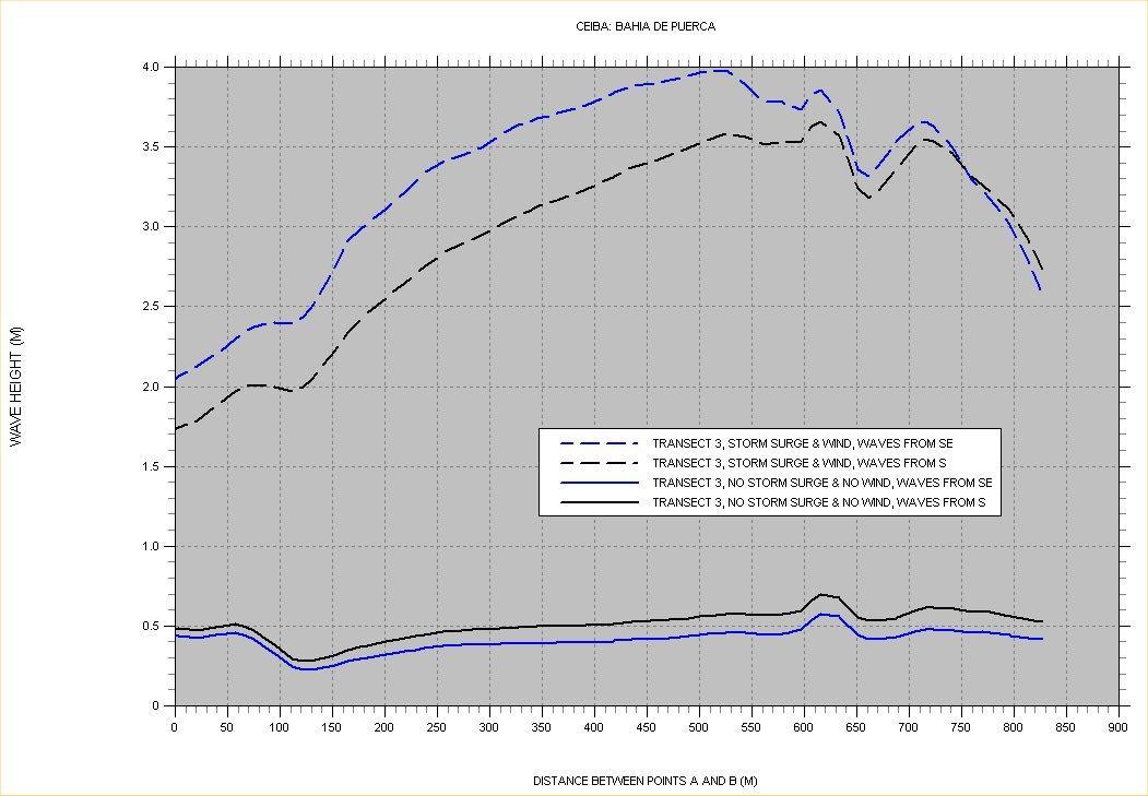
penetrate deep into the back bay. And Figure 62 shows that Bahía de Puerca is even more exposed, allowing waves larger than 3.5 m to reach well inside. Both figures show the largest heights occurring on the entrance channels.
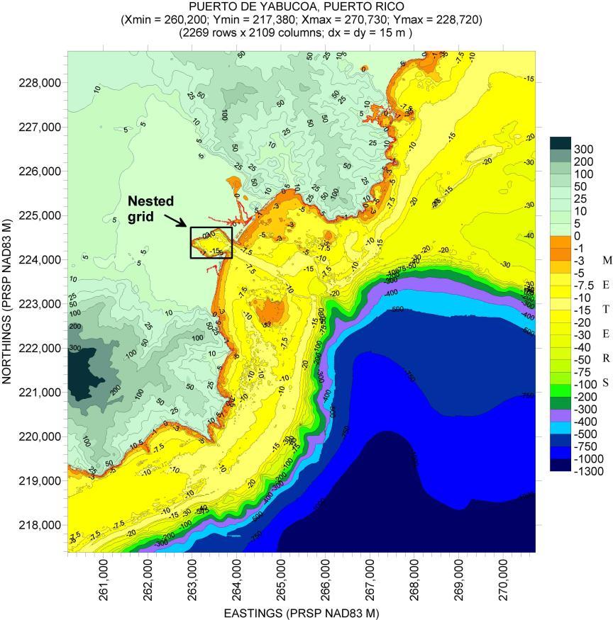
PUERTO DE YABUCOA
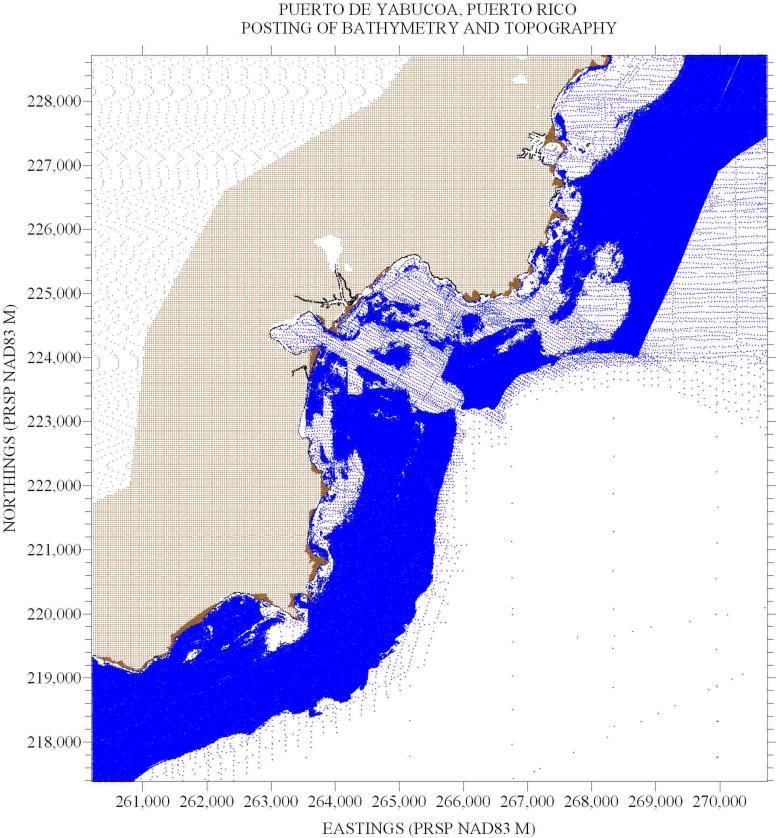
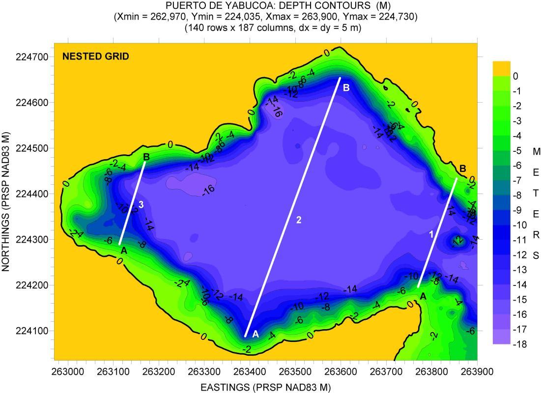
Figure 63 shows a posting of the locations where bathymetry and topography values are available for the computational grid. Figure 64 shows a depth contour plot for the computational grid. Also shown is the outline of the nested grid. Figure 65 shows a depth contour plot of the nested grid. Also shown is the location where Hs slices will be taken.
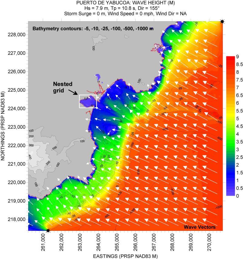
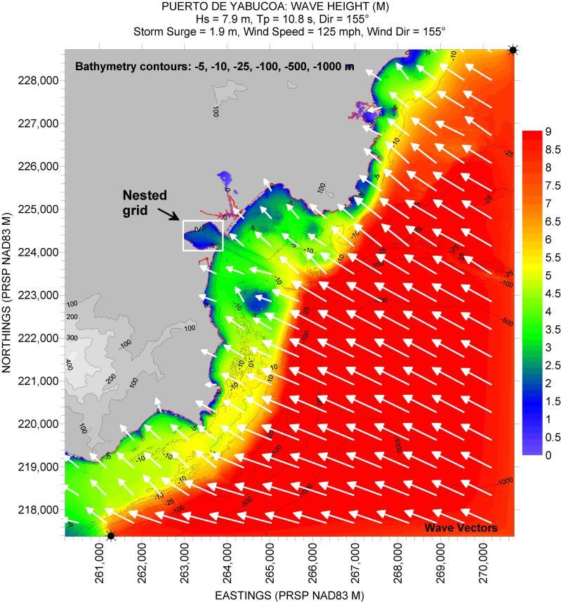
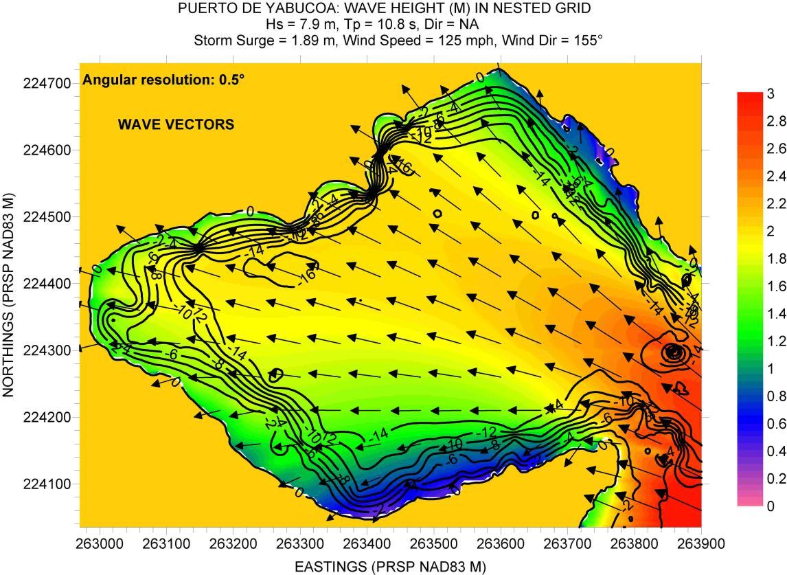
Only one wave and wind direction was run for this case since it is obvious that the worst scenario will be for waves aligned with the wind, both coming from a southeasterly direction along the entrance channel. Figure 66 shows the Hs field for the case of no storm surge and no wind, and Figure 67 shows the results for the nested grid Figure 68 shows the results for the scenario of both storm surge and wind forcing, and Figure 69 shows the corresponding results for the nested grid.
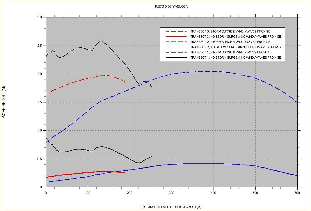
Figure 70 shows that the port is well protected under no wind conditions. But once strong winds are aligned with the entrance channel then waves close to 2 m in height can be expected inside. It should be noticed that while Transect 2 and 3 results with no wind are basically the same in wave heights, once wind starts blowing the results for Transect 3 (farther inside the port) become larger than for Transect 2. This implies that the difference is due to the longer fetch for Transect 3 (relative to the port entrance) and, hence, to local effects.
63. Posting showing location of bathymetry and topography values for Puerto de Yabucoa.
Figure 64. Depth contour plot of the outer computational grid for Puerto de Yabucoa. Outline of nested grid also shown.
Figure
plot
based on the scenario listed along the top margin of figure.
Figure 65. Depth contour plot of nested grid for Puerto Las Mareas.
Figure 66. Hs contour
for Puerto de Yabucoa,
67. Hs contour plot for (nested) Puerto
based on the scenario listed along the top margin of the figure.
68. Hs contour plot for Puerto
based on the scenario listed along the top margin of the figure.
Figure
de Yabucoa,
Figure
de Yabucoa,
Figure 69. Hs contour plot for (nested) Puerto de Yabucoa, based on the scenario listed along the top margin of figure.
Figure 70. Significant wave height “slices” for Puerto de Yabucoa.
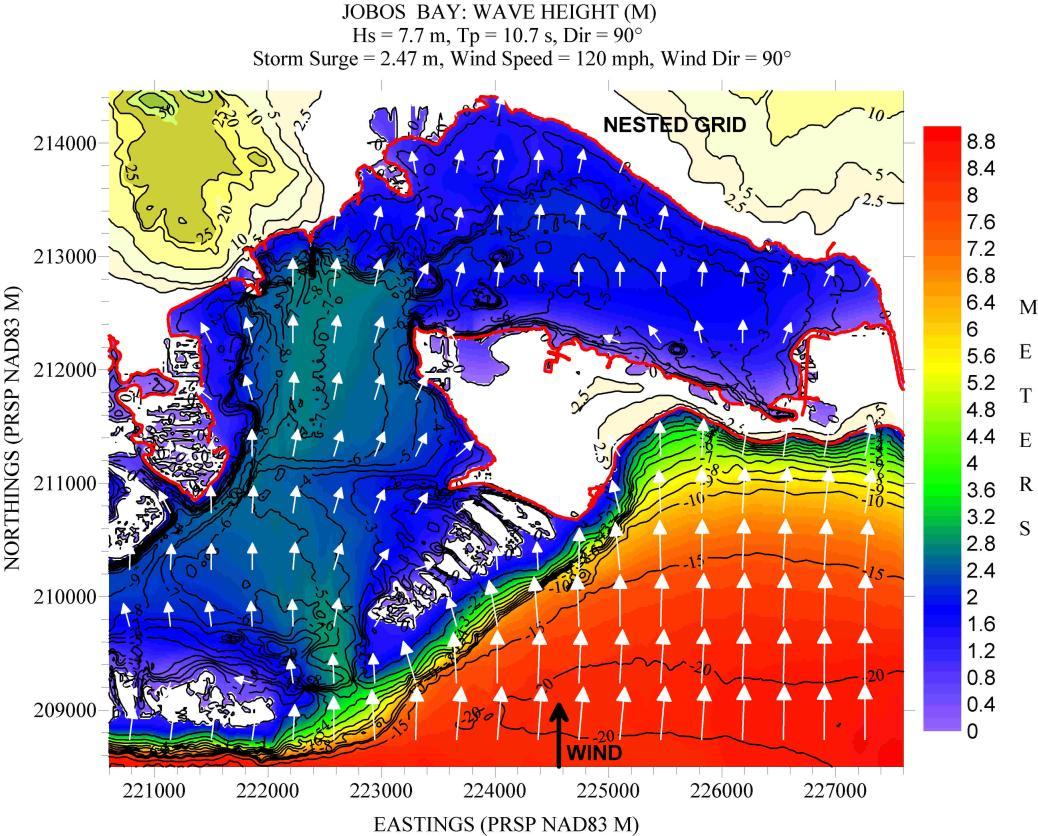
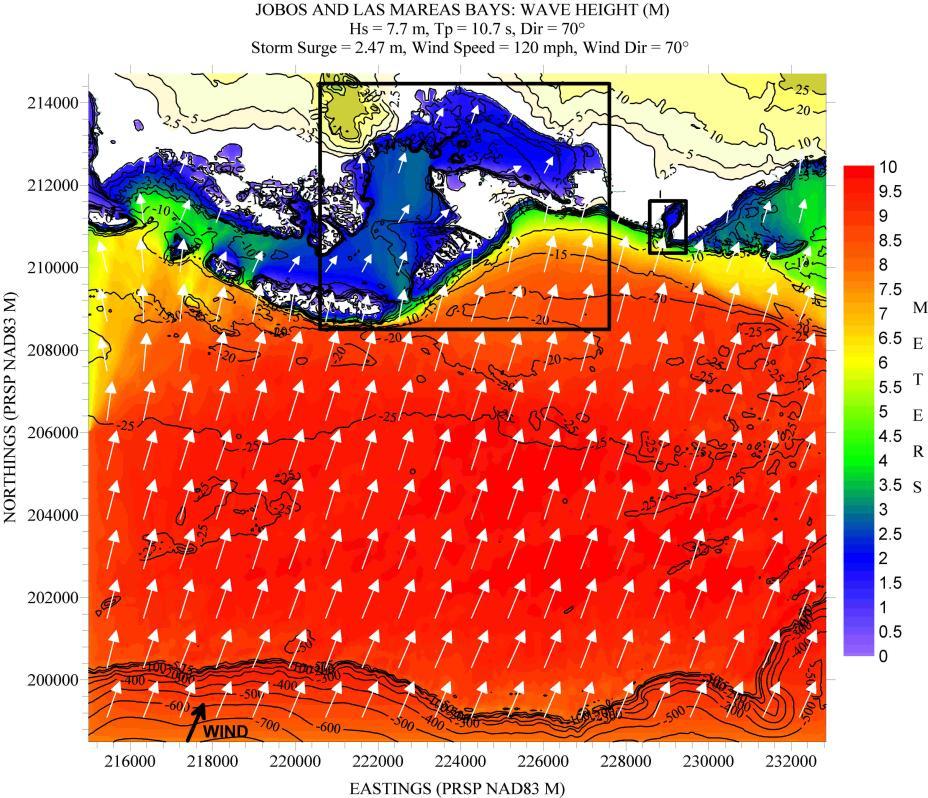
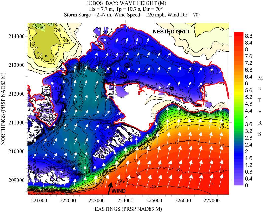
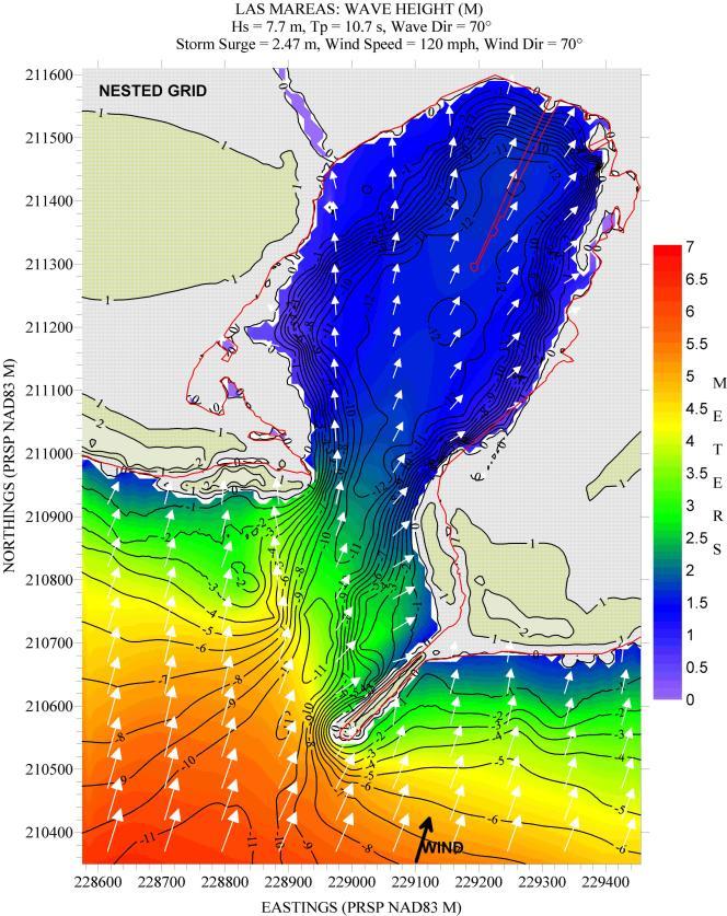
JOBOS BAY & PUERTO LAS MAREAS
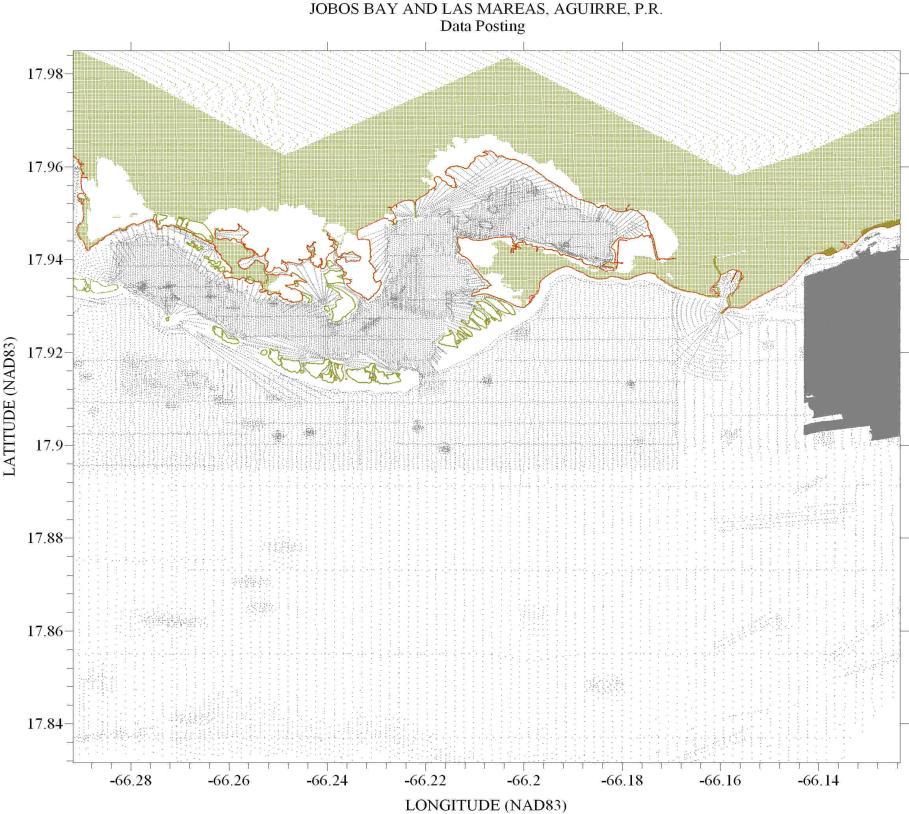
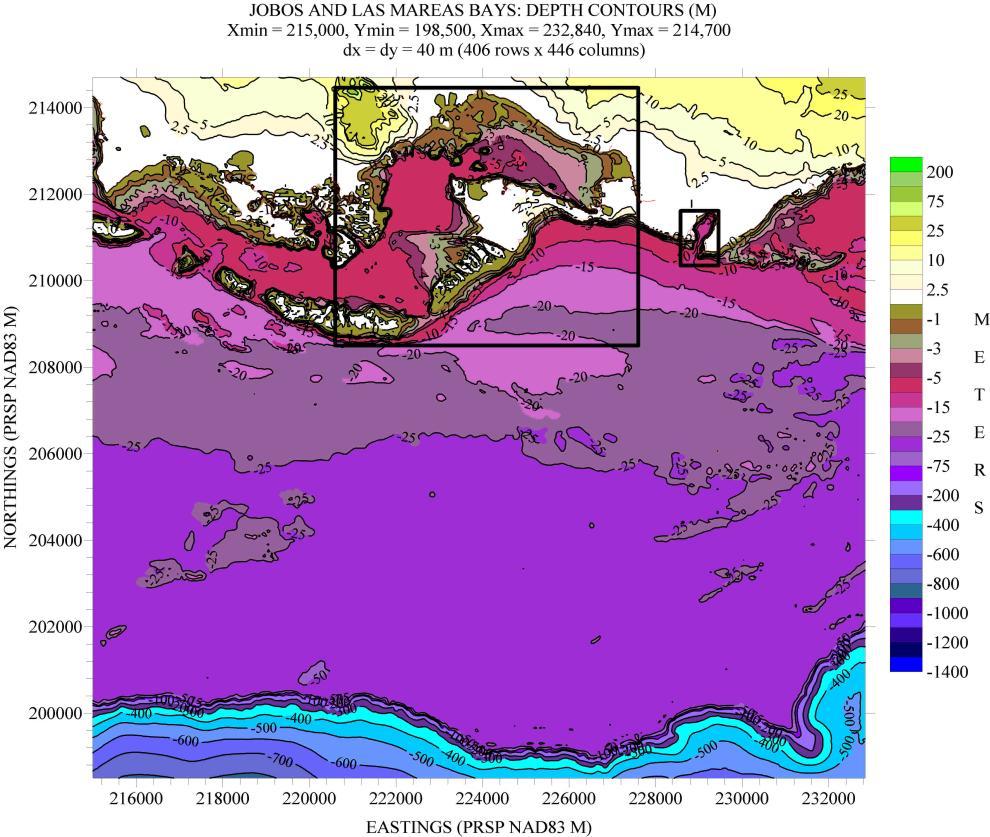
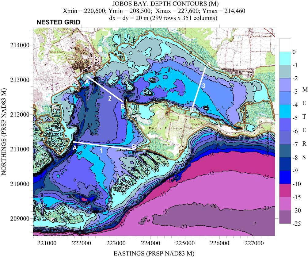
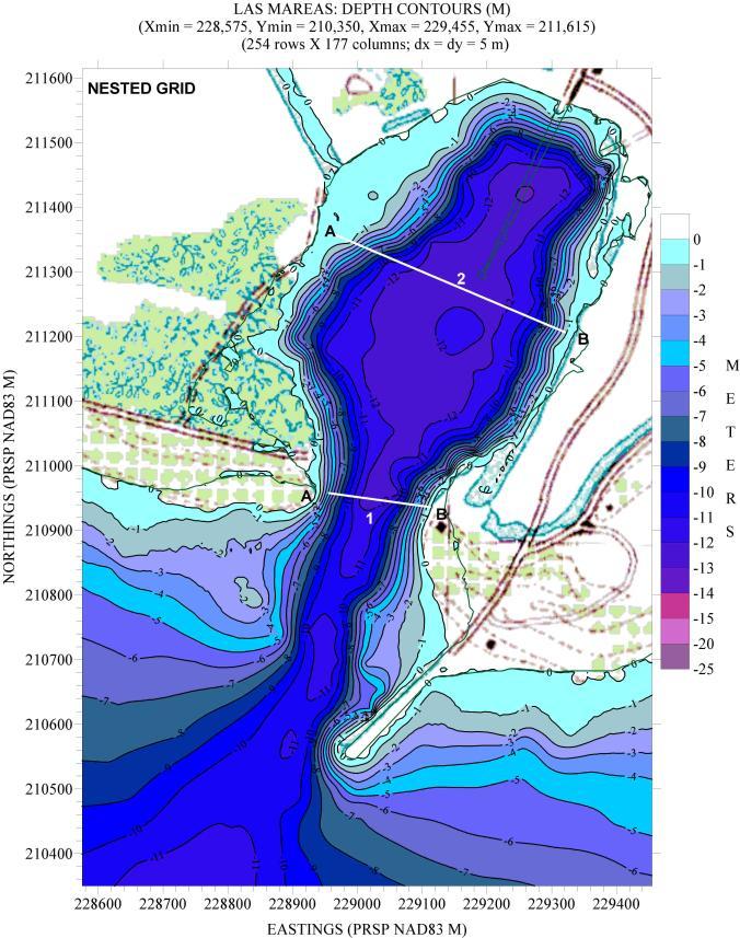
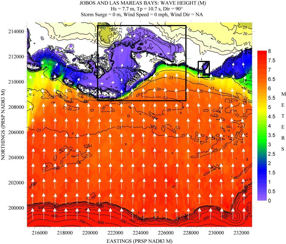
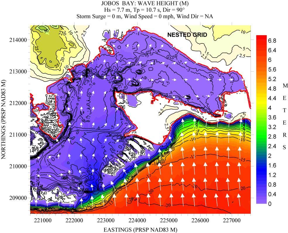
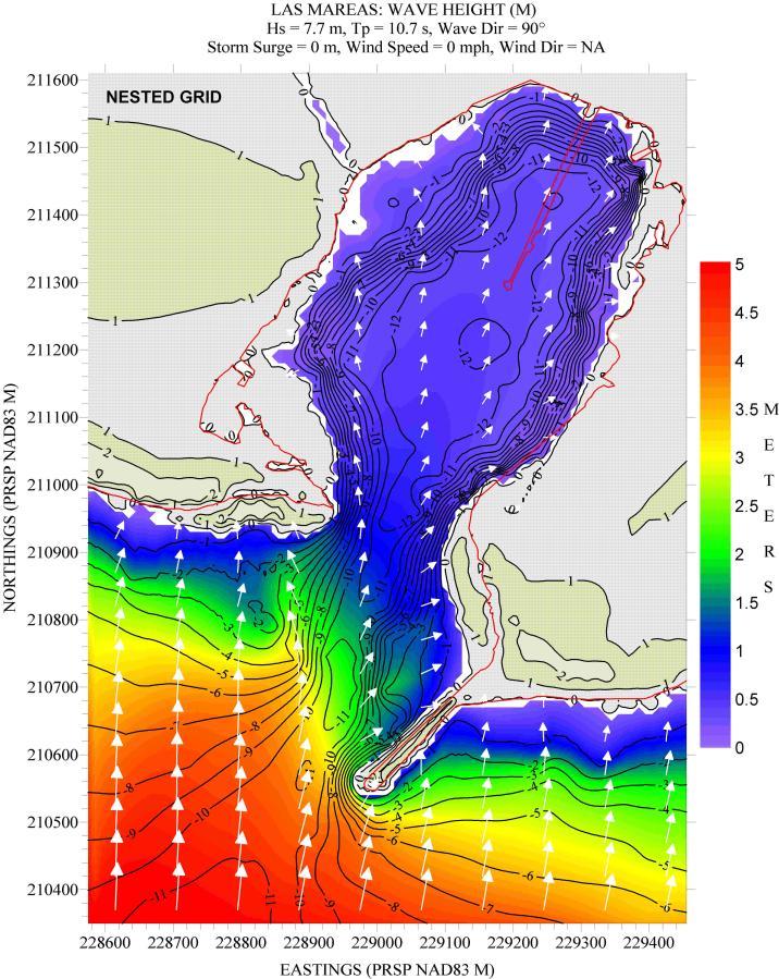
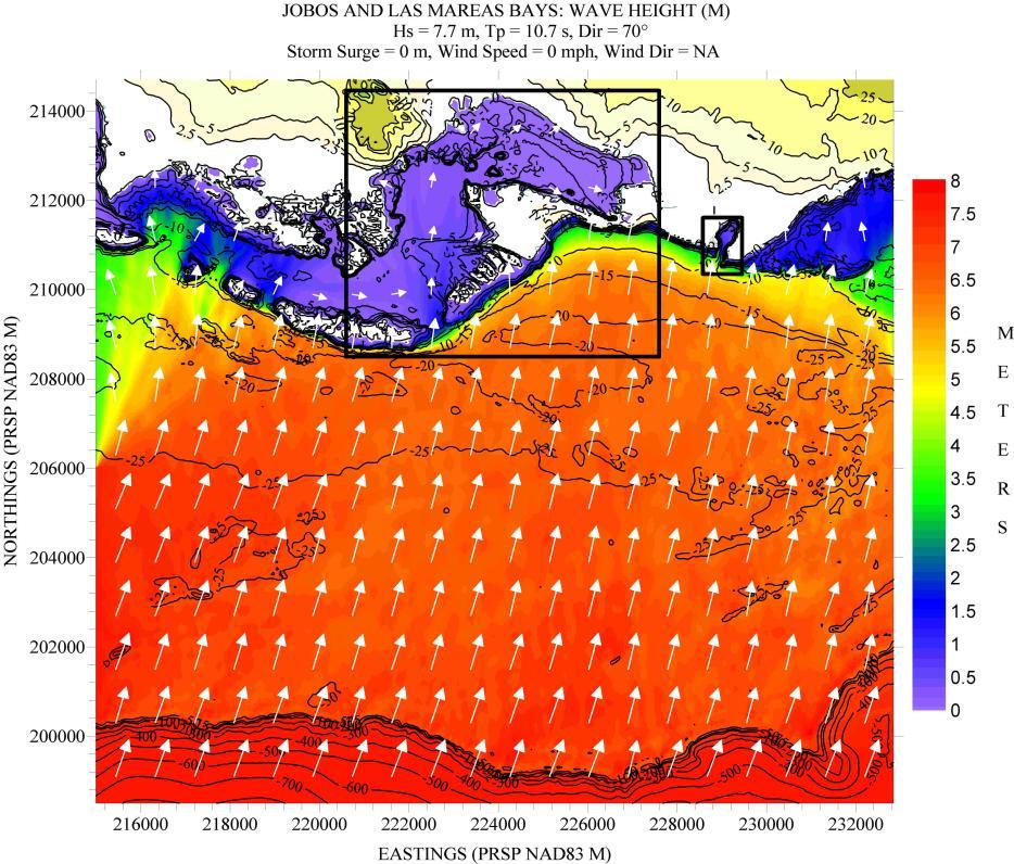
Figure 71 shows a posting of the bathymetry and topography data points. As mentioned above, from this location westward the SHOALS (nor another attempt by the USGS) worked, so along the south coast we will be using NOS ship data from the 1960’s and 1970’s. Figure 72 shows a depth contour plot for the outer computational grid, also showing the outline of the two nested grids for Jobos Bay (largest) and Puerto Las Mareas (smallest). Figures 73 and 74 show depth contour plots for the two nested grids. The figures also show the transects along which the Hs slices are going to be taken.
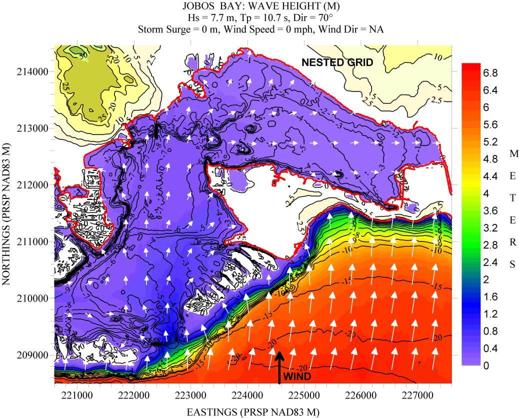
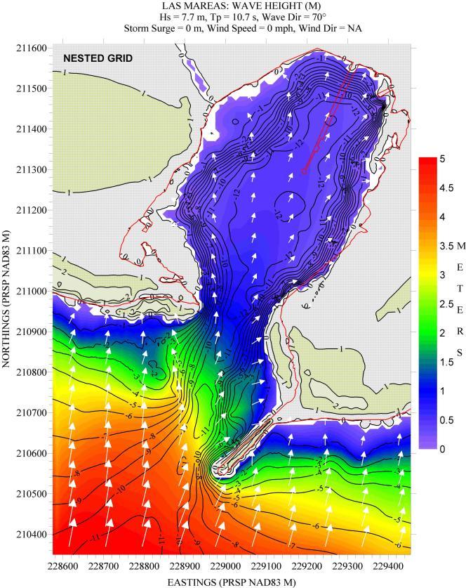
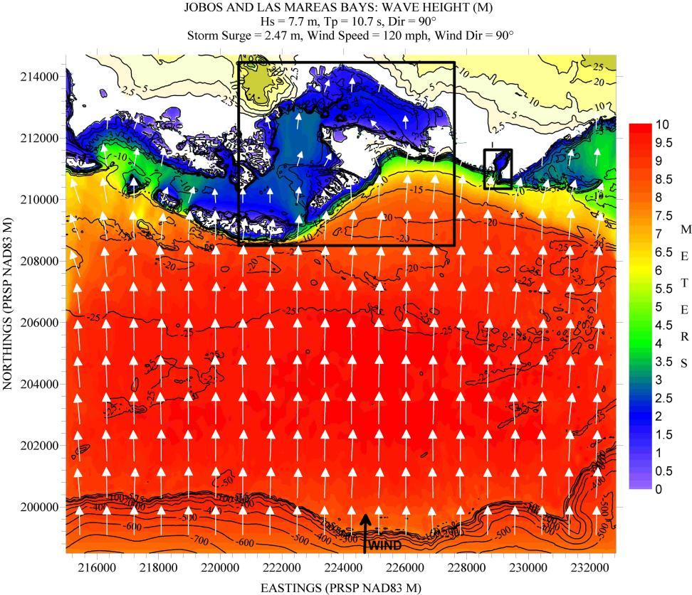
Figures 75 to 86 show the results for these locations Both locations are well protected from waves from offshore, in the Jobos Bay case by the offshore chain of low-lying mangrove islands, and in the Las Mareas case by the choke imposed by the narrow entrance.
Jobos Bay:
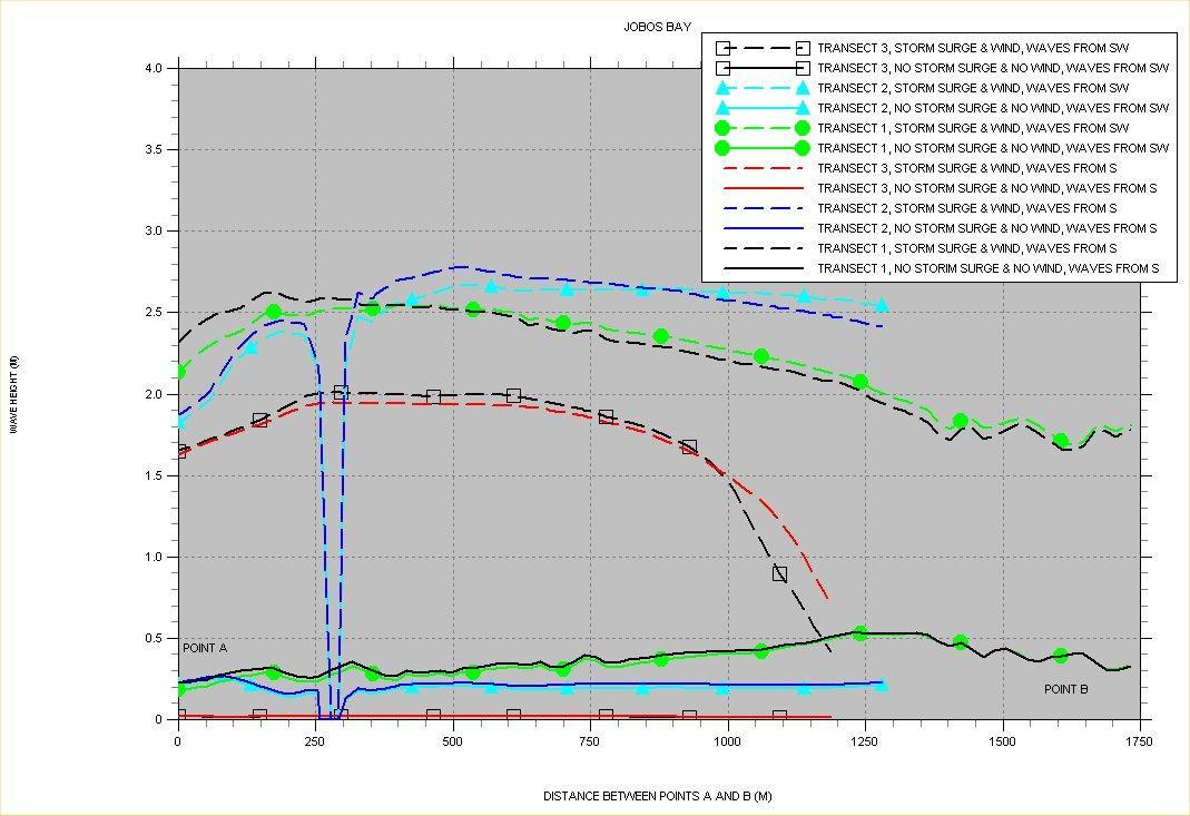
In Jobos, once you add a storm surge and wind then waves become higher, or equal to, 2 m inside the bay, even in the transect further inside the bay (#3). The western side of Transect 1 (near Point A) is more exposed due to the wider inter-island gap among the protecting offshore islands.
Puerto Las Mareas:
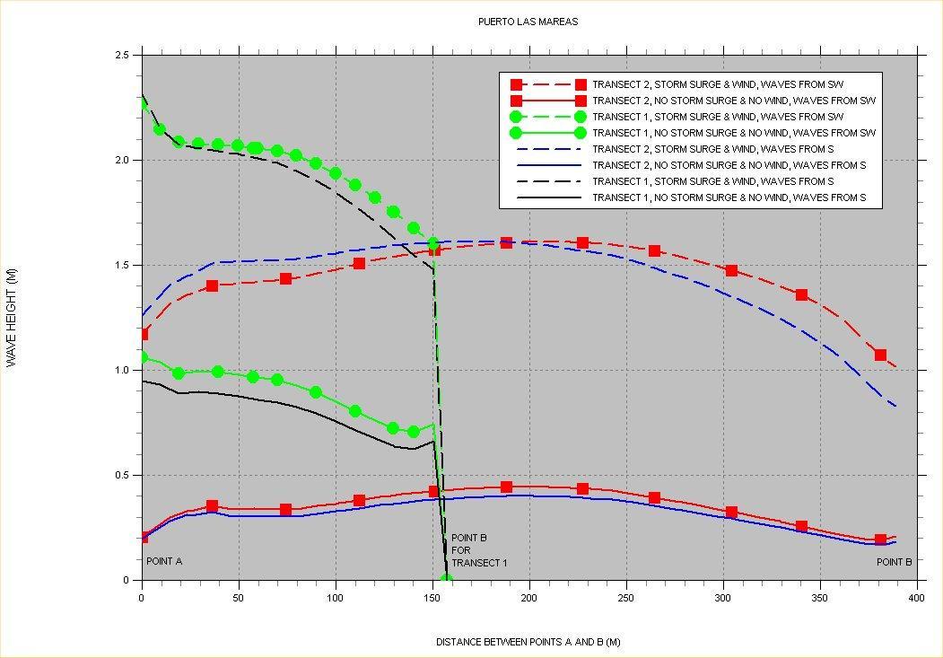
Las Mareas is well protected due to its narrow entrance, with the highest waves on the order of 1.5 m well inside the port even under wind and storm surge conditions. And the entrance jetty seems to also play a role in the protection since it trends towards the southwest.
71. Posting showing location of bathymetry and topography values for Jobos Bay and Puerto Las Mareas.
Figure
Figure 72. Depth contour plot of the outer computational grid for Jobos Bay and Puerto Las Mareas. Outline of nested grids also shown.
Figure 73. Depth contour plot of nested grid for Jobos Bay.
Figure 74. Depth contour plot of nested grid for Puerto Las Mareas.
Figure 75. Hs contour plot for Jobos Bay and Puerto Las Mareas, based on the scenario listed along the top margin of figure.
Figure 76. Hs contour plot for (nested) Jobos Bay, based on the scenario listed along the top margin of figure.
Figure 77. Hs contour plot for (nested) Puerto Las Mareas, based on the scenario listed along the top margin of figure.
Figure 78. Hs contour plot for Jobos Bay and Puerto Las Mareas, based on the scenario listed along the top margin of figure.
Figure 79. Hs contour plot for (nested) Jobos Bay, based on the scenario listed along the top margin of figure.
Figure 80. Hs contour plot for (nested) Puerto Las Mareas, based on the scenario listed along the top margin of figure.
Figure 81. Hs contour plot for Jobos Bay and Puerto Las Mareas, based on the scenario listed along the top margin of figure.
Figure 82. Hs contour plot for (nested) Jobos Bay, based on the scenario listed along the top margin of figure.
Figure 83. Hs contour plot for (nested) Puerto Las Mareas, based on the scenario listed along the top margin of figure.
Figure 84. Hs contour plot for Jobos Bay and Puerto Las Mareas, based on the scenario listed along the top margin of figure.
Figure 85. Hs contour plot for (nested) Jobos Bay, based on the scenario listed along the top margin of figure.
Figure 86. Hs contour plot for (nested) Puerto Las Mareas, based on the scenario listed along the top margin of figure.
Figure 87. Significant wave height “slices” for Jobos Bay.
Figure 88. Significant wave height “slices” for Puerto Las Mareas.
PONCE BAY
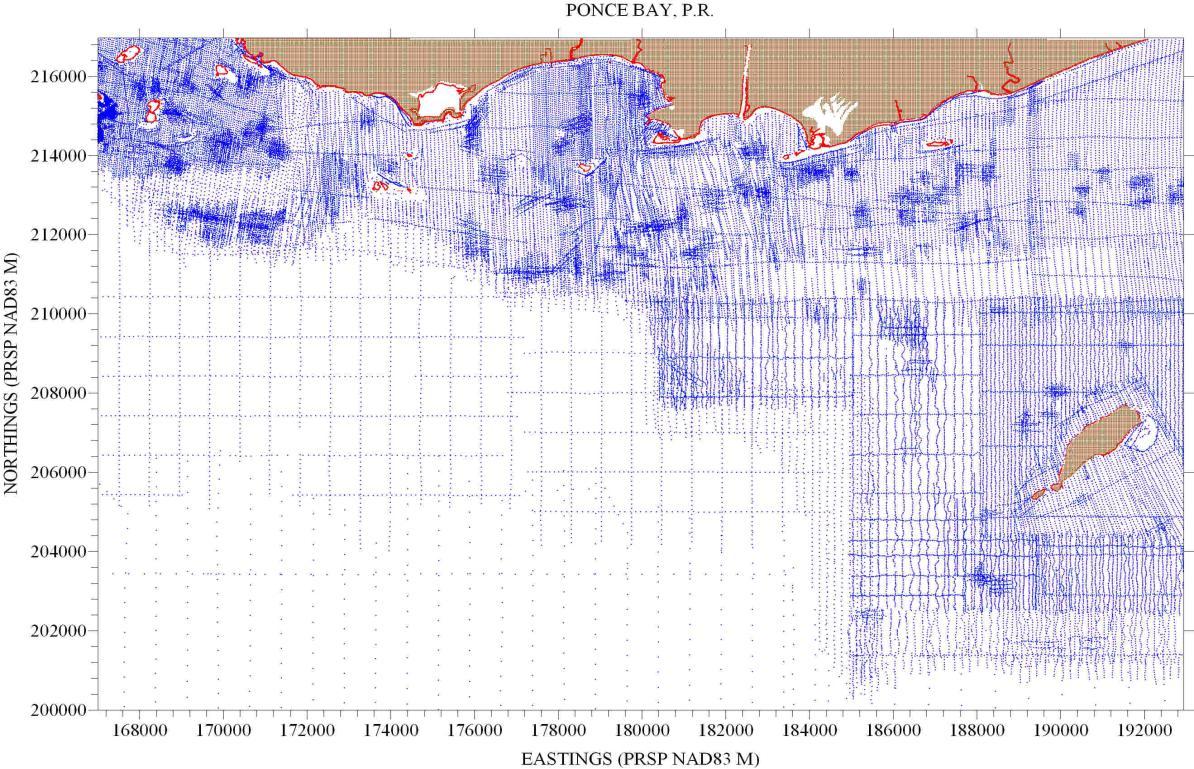
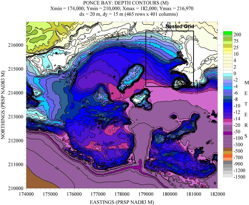
Figure 89 shows a posting of the bathymetry and topography data values. Figure 90 shows a depth contour plot of the outer computational grid, and the outline of the nested grid. Figure 91 shows the depth contour plot of the nested grid, and the “slice” along which Hs values are taken.
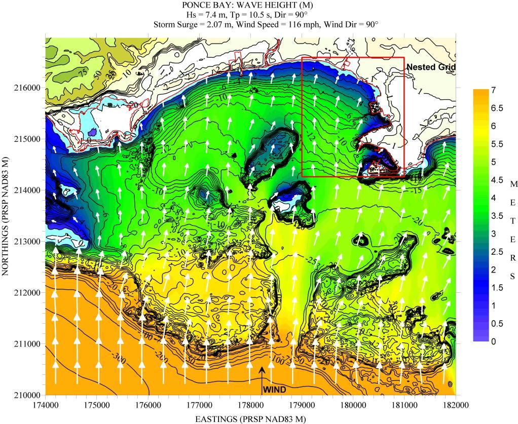
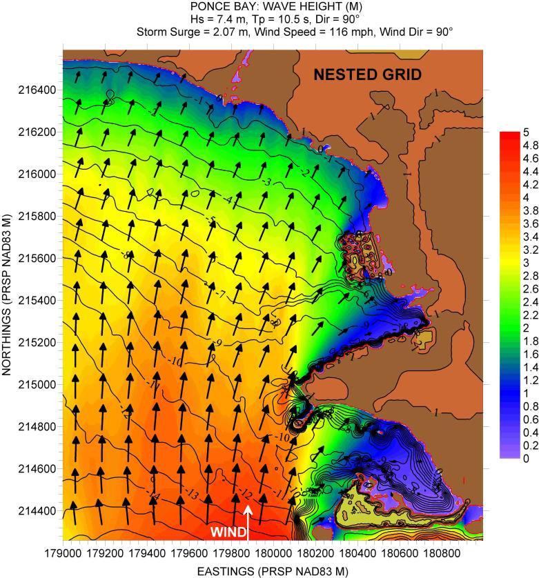
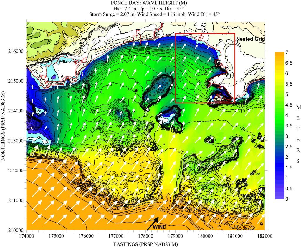
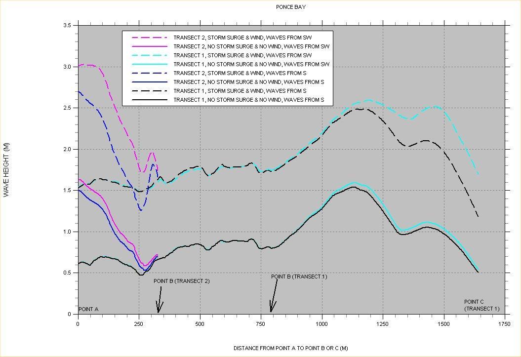
Figures 92 to 99 show contour plots of the Hs field for the simulations carried out and described along the top margin of each figure. The results shown in Figure 100 for Transect 1 show that the bay is relatively well protected between Points A and B, basically because of its shallow depths. Under storm conditions wave heights increase to more than 2 m between Points B and C , which is mainly a reflection of the increasing depth along these two points. Transect 2 shows this section to be exposed to very large waves under storm conditions. In deeper waters inside the bay wave heights can become higher than 3 m under storm conditions (see Figures 97 and 99). Thus Ponce Bay is relatively well exposed due to the fact that under hurricane conditions we can expect waves on the order of 3 m to penetrate well inside the bay in its deeper areas.
Figure 89. Posting showing location of bathymetry and topography values for Ponce Bay.
90. Depth contour plot of outer computational grid for Ponce Bay. Also shown is the outline of the nested grid.
Figure
scenario listed along the top margin of figure.
Figure 91. Depth contour plot of nested computational grid for Ponce Bay.
Figure 92. Hs contour plot for Ponce Bay, based on the
Figure 93. Hs contour plot for (nested) Ponce Bay, based on the scenario listed along the top margin of figure.
Figure 94. Hs contour plot for Ponce Bay, based on the scenario listed along the top margin of figure.
Figure 95. Hs contour plot for (nested) Ponce Bay, based on the scenario listed along the top margin of figure.
Figure 96. Hs contour plot for Ponce Bay, based on the scenario listed along the top margin of figure.
Figure 97. Hs contour plot for (nested) Ponce Bay, based on the scenario listed along the top margin of figure.
Figure 98. Hs contour plot for Ponce Bay, based on the scenario listed along the top margin of figure.
99. Hs contour plot for (nested) Ponce Bay, based on the scenario listed along the top margin of figure.
Figure
Figure 100. Significant wave height “slices” for Ponce Bay.
GUAYANILLA BAY
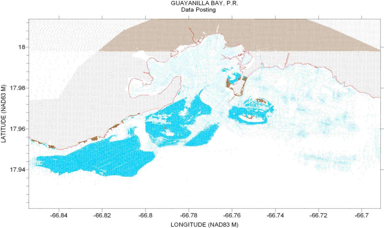
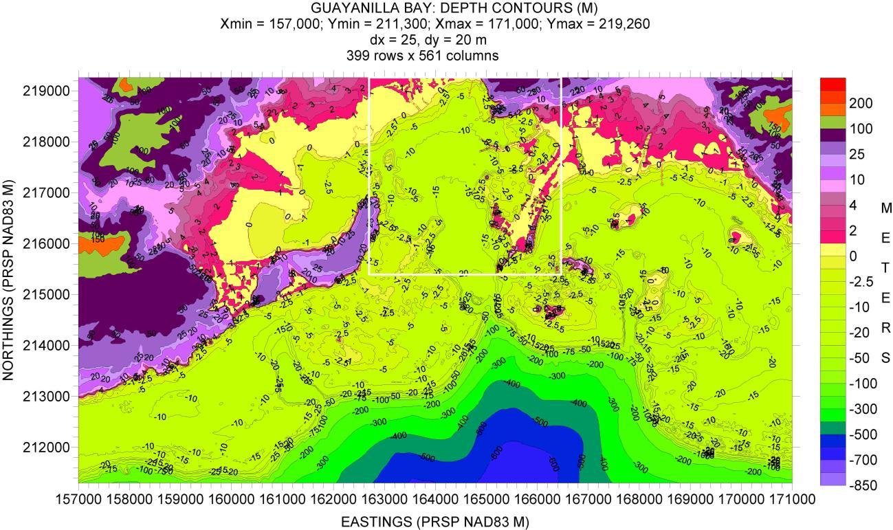
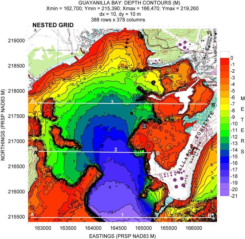
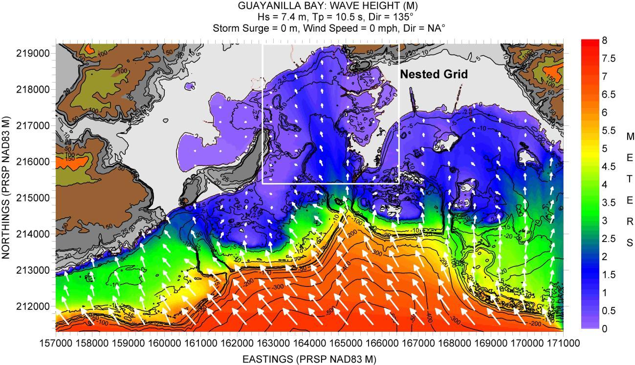
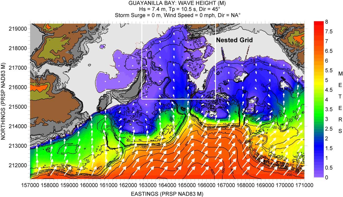
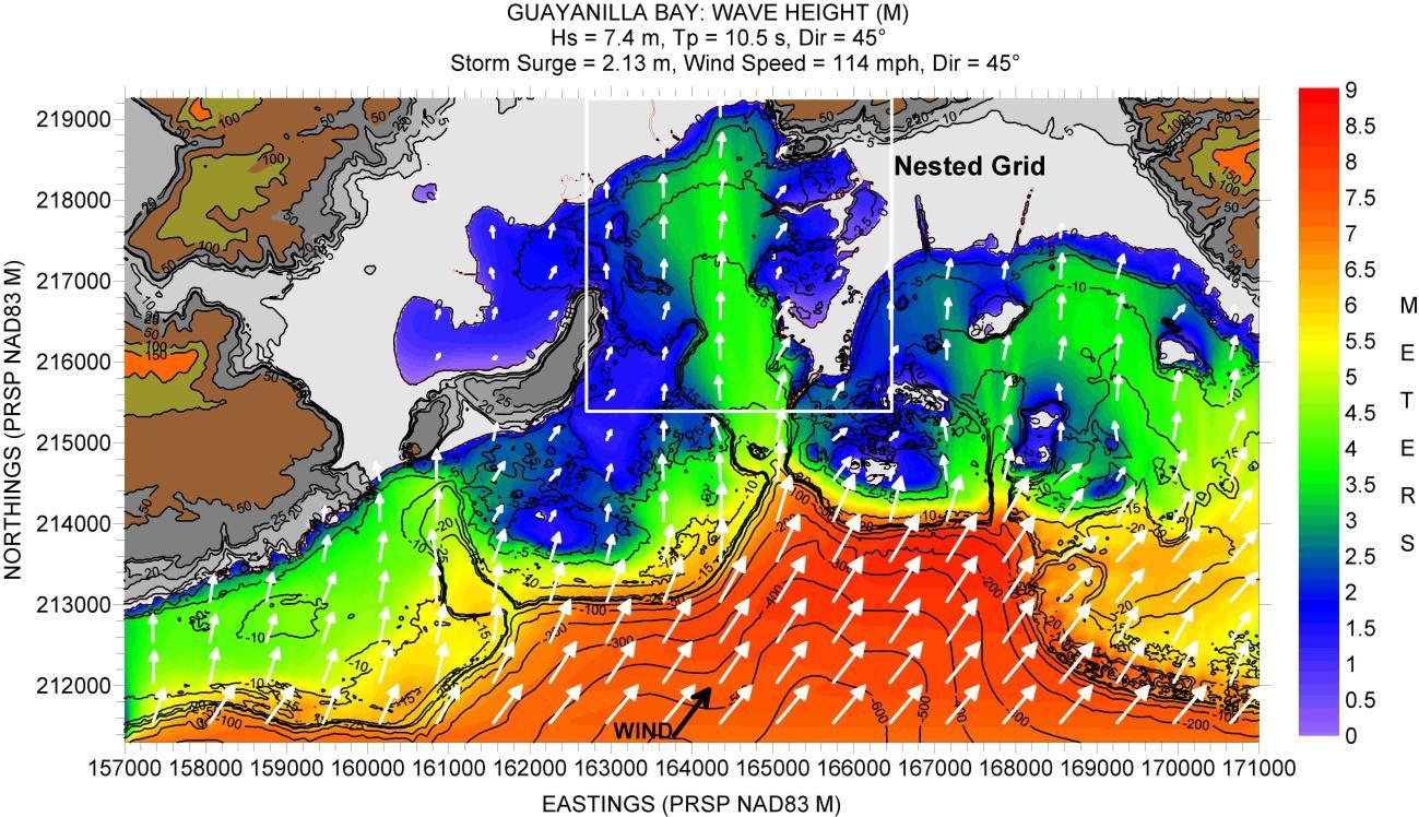
Figure 101 shows a posting of the locations for the bathymetry and topography values. Figure 102 shows a depth contour plot of the computational grid, and also shows the outline of the nested grid. Figure 103 shows a depth contour plot of the nested grid computational grid, including the location of the “slices” to be used.
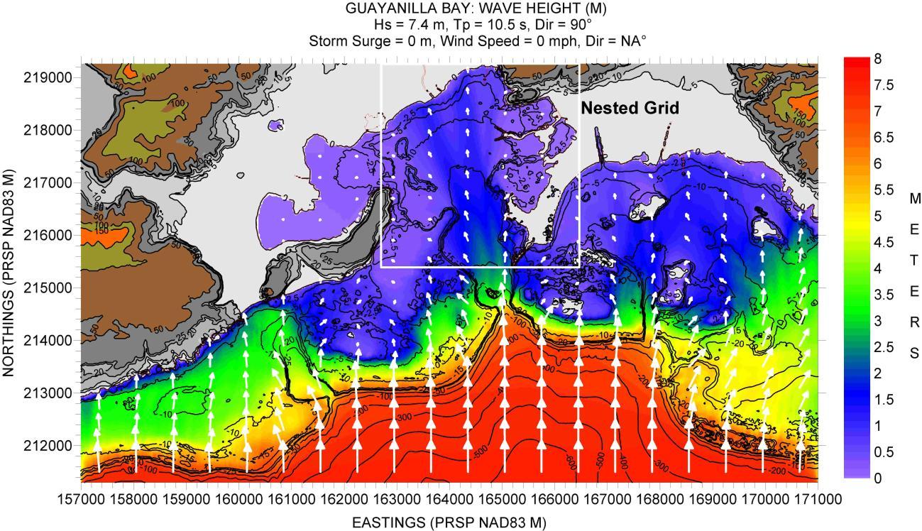
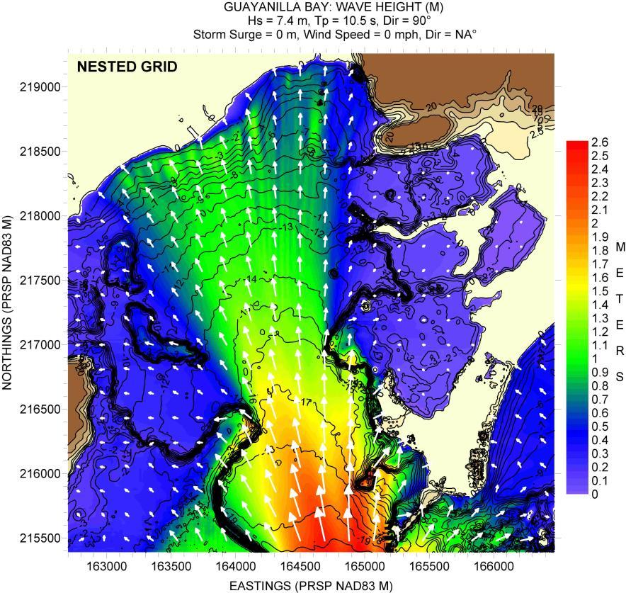
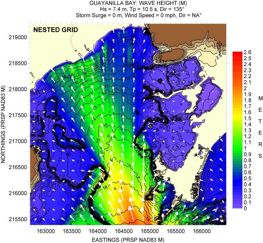
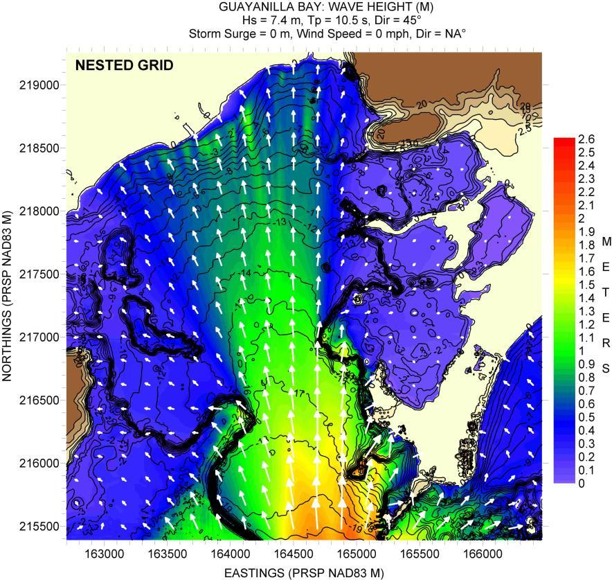
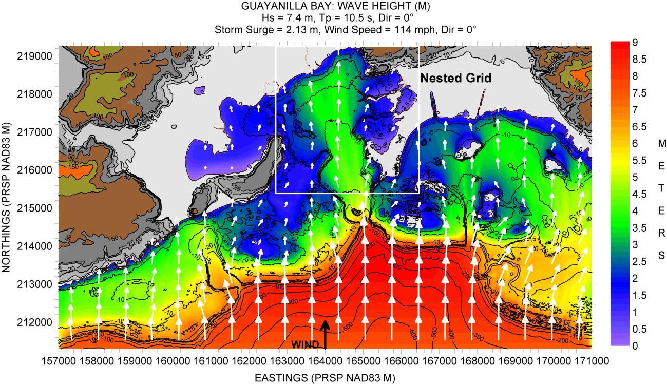
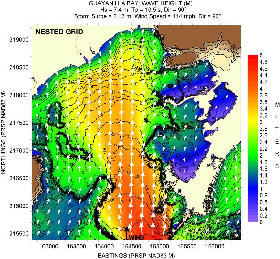
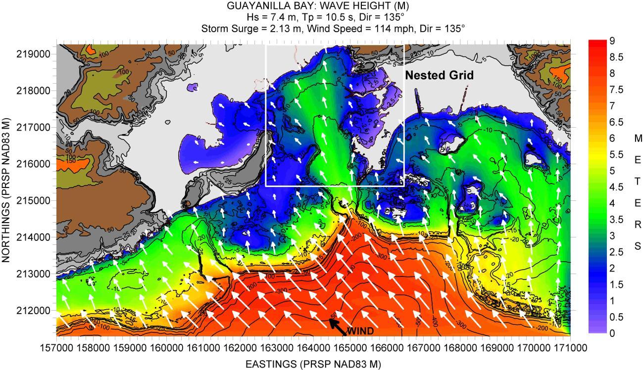
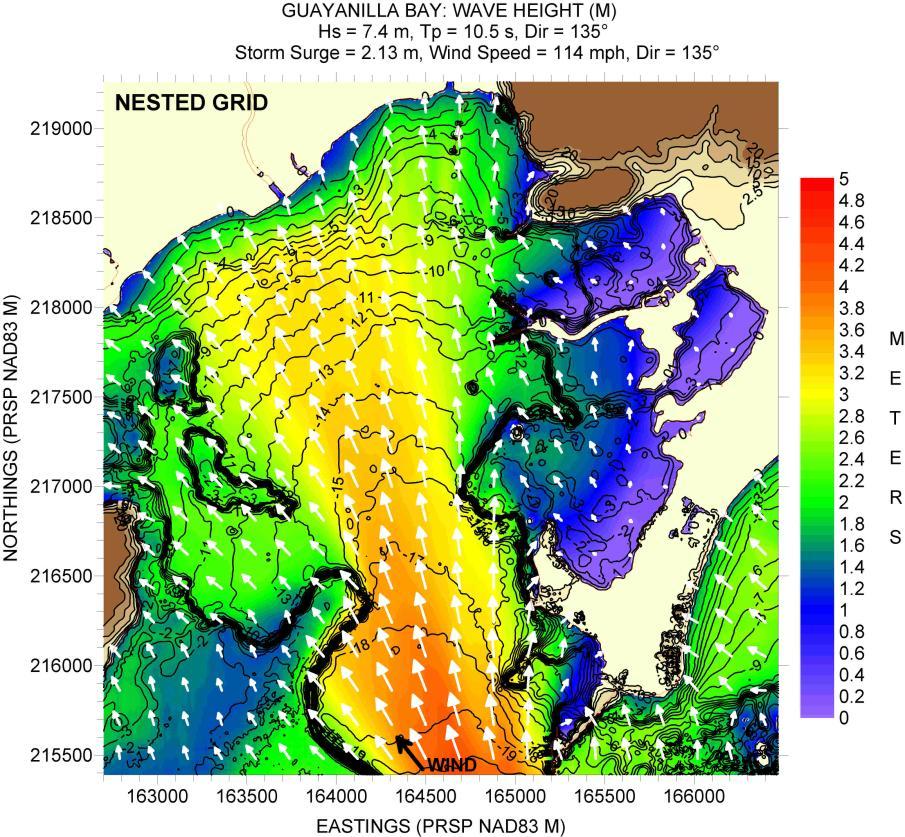
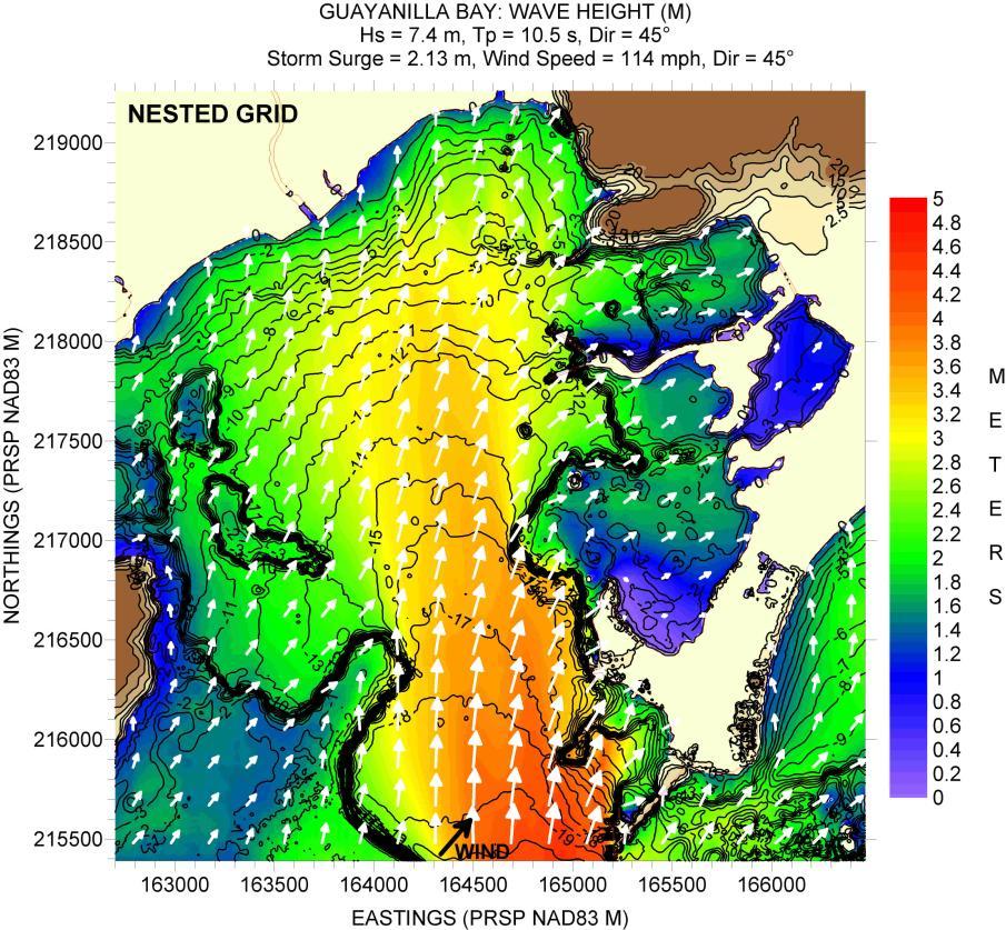
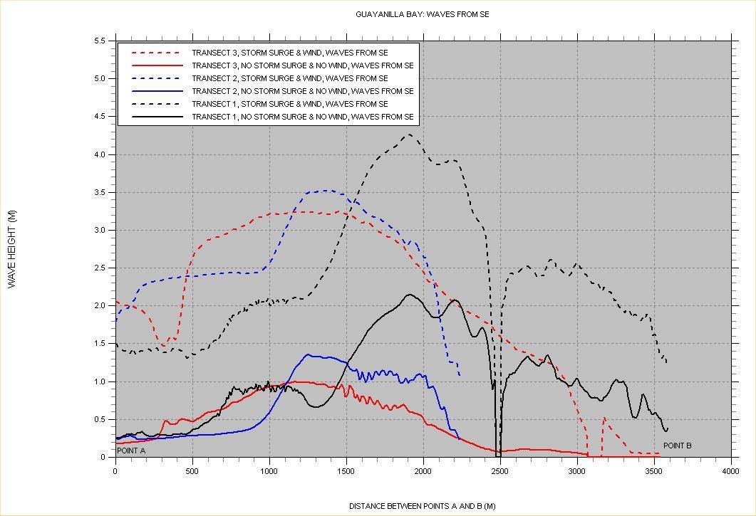
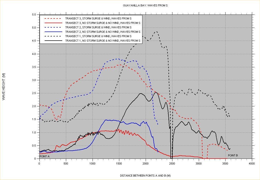
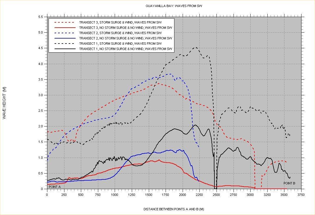
Figures 104 to 115 show contour plots of the Hs field for the simulations carried out and described along the top margin of each figure. This bay is another good example of how the entrance channel facilitates wave energy penetration into the bay. Figures 116, 117, and 118 show the results from the three slices shown in Figure 103, from the southeast, south, and southwest, respectively. The figures show that once inside the bay, the wave field is practically the same no matter the deepwater wave direction. For this bay the shelf break lies close to the bay entrance. We can see large waves (≥ 3 m) penetrating deep inside the bay under wind and storm surge conditions, along the deeper parts of the bay. It is only in the eastern side of the bay, sheltered by Punta Guayanilla and in shallower waters, that some protection can be seen. Waves from the south seem to produce the highest waves inside the bay.
101. Posting showing location of bathymetry and topography values for Guayanilla Bay.
computational grid for
Figure
Figure 102. Depth contour plot of
Guayanilla Bay.
103. Depth contour plot for nested computational grid. Also shown are the locations where Hs “slices” will be acquired.
104. Hs contour plot for Guayanilla Bay, based on the scenario listed along the top margin of figure.
Figure
Figure
Figure 105. Hs contour plot for (nested) Guayanilla Bay, based on the scenario listed along the top margin of figure.
Figure 106. Hs contour plot for Guayanilla Bay, based on the scenario listed along the top margin of figure.
Figure 107. Hs contour plot for (nested) Guayanilla Bay, based on the scenario listed along the top margin of figure.
Figure 108. Hs contour plot for Guayanilla Bay, based on the scenario listed along the top margin of figure.
Figure 109. Hs contour plot for (nested) Guayanilla Bay, based on the scenario listed along the top margin of figure.
Figure 110. Hs contour plot for Guayanilla Bay, based on the scenario listed along the top margin of figure.
Figure 111. Hs contour plot for (nested) Guayanilla Bay, based on the scenario listed along the top margin of figure.
Figure 112. Hs contour plot for Guayanilla Bay, based on the scenario listed along the top margin of figure.
Figure 113. Hs contour plot for (nested) Guayanilla Bay, based on the scenario listed along the top margin of figure.
Figure 114. Hs contour plot for Guayanilla Bay, based on the scenario listed along the top margin of figure.
Figure 115. Hs contour plot for (nested) Guayanilla Bay, based on the scenario listed along the top margin of figure.
Figure 116. Significant wave height “slices” for Guayanilla Bay. Waves from the southeast.
Figure 117. Significant wave height “slices” for Guayanilla Bay. Waves from the south.
Figure 118. Significant wave height “slices” for Guayanilla Bay. Waves from the southwest.
GUANICA BAY
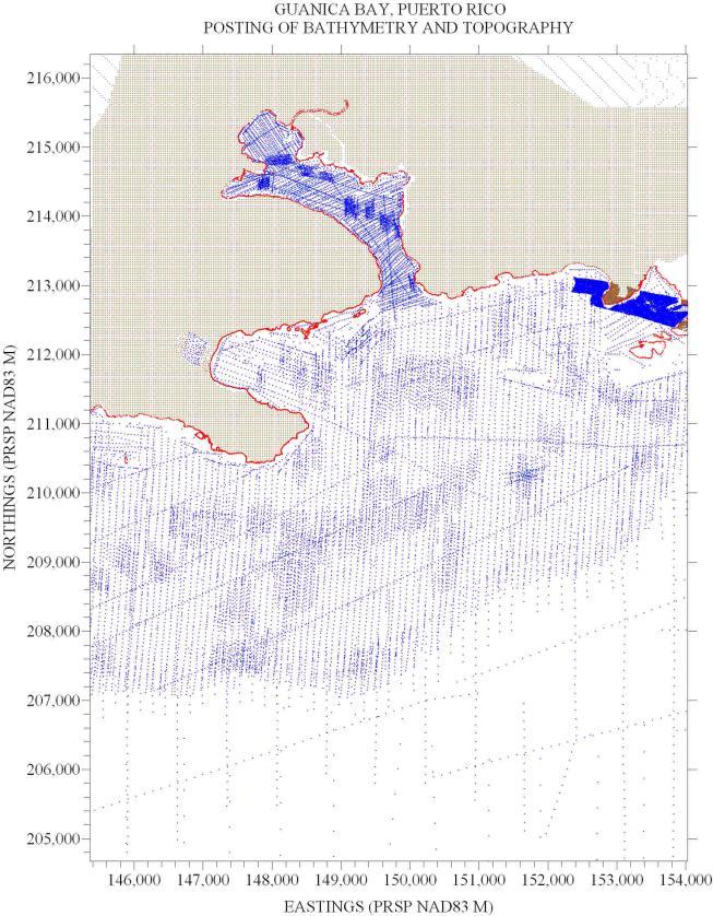
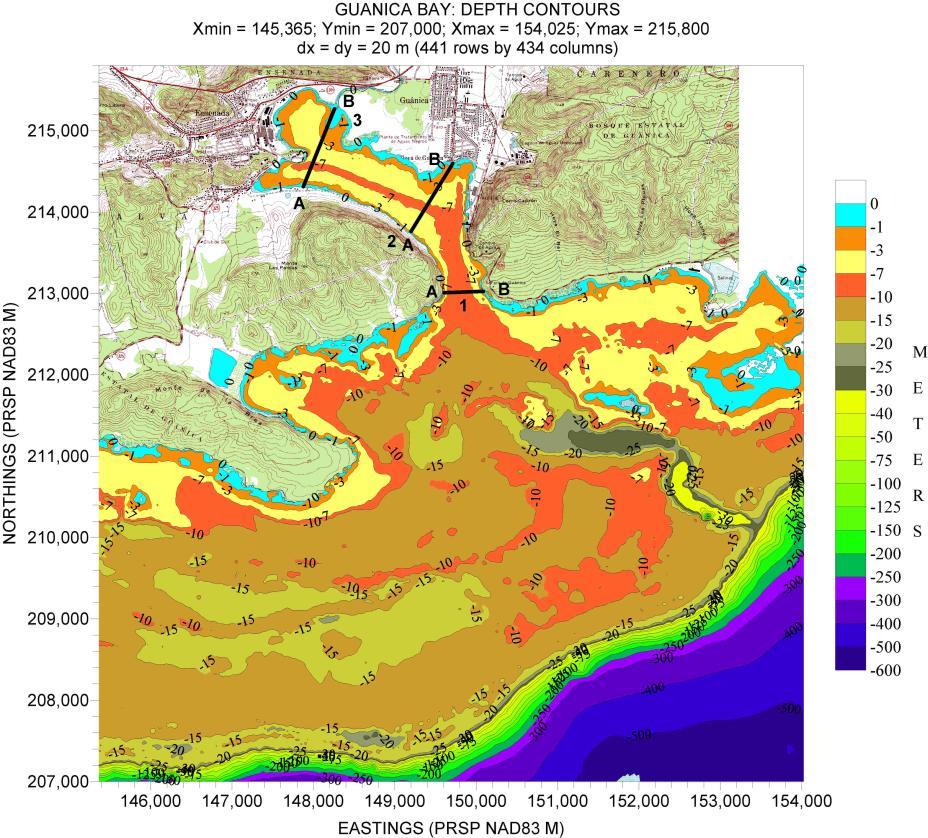
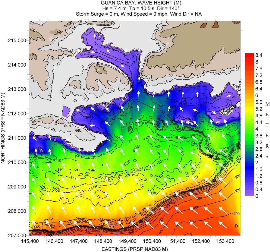
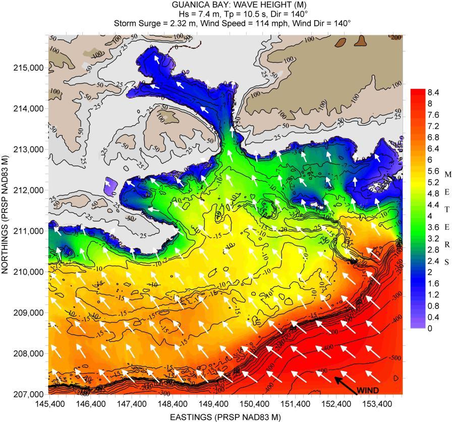
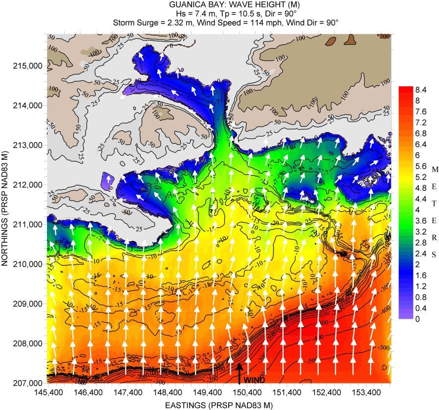
Figure 119 shows a posting of the locations of bathymetry and topography values. Figure 120 shows a depth contour plot of the computational grid, and also the locations where “slices” of Hs will be taken. Figures 121 to 124 show the results for offshore waves propagating from the southeast and south. The southeast direction was chosen since wind blowing from that direction will blow along the long axis inside the bay. The figures show how the long and narrow entrance chokes the propagation of wave energy coming from the outside, even under storm surge and wind conditions.
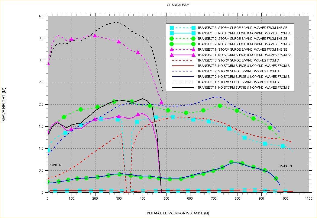
Figure 125 shows the Hs values along the slices. The figure shows the bay is relatively well protected even under storm surge and wind conditions. The long and narrow entrance cuts-off almost all of the wave energy received at Transect 1. Near Point B of Transect 2, under wind from the south, only waves of 1.5 m are observed just offshore of the Guanica town “malecón” (or seawall). Deep inside the bay (Transect 3) waves on the order of 1.5 m are observed as a maximum.
119. Posting showing location of bathymetry and topography values for Guanica Bay.
Figure
Figure 120. Depth contour plot of computational grid for Guanica Bay.
Figure 121. Hs contour plot for Guanica Bay, based on the scenario listed along the top margin of figure.
Figure 122. Hs contour plot for Guanica Bay, based on the scenario listed along the top margin of figure.
Figure 123. Hs contour plot for Guanica Bay, based on the scenario listed along the top margin of figure.
Figure 124. Hs contour plot for Guanica Bay, based on the scenario listed along the top margin of figure.
Figure 125. Significant wave height “slices” for Guanica Bay.
BOQUERON BAY AND PUERTO REAL
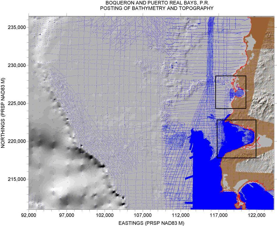
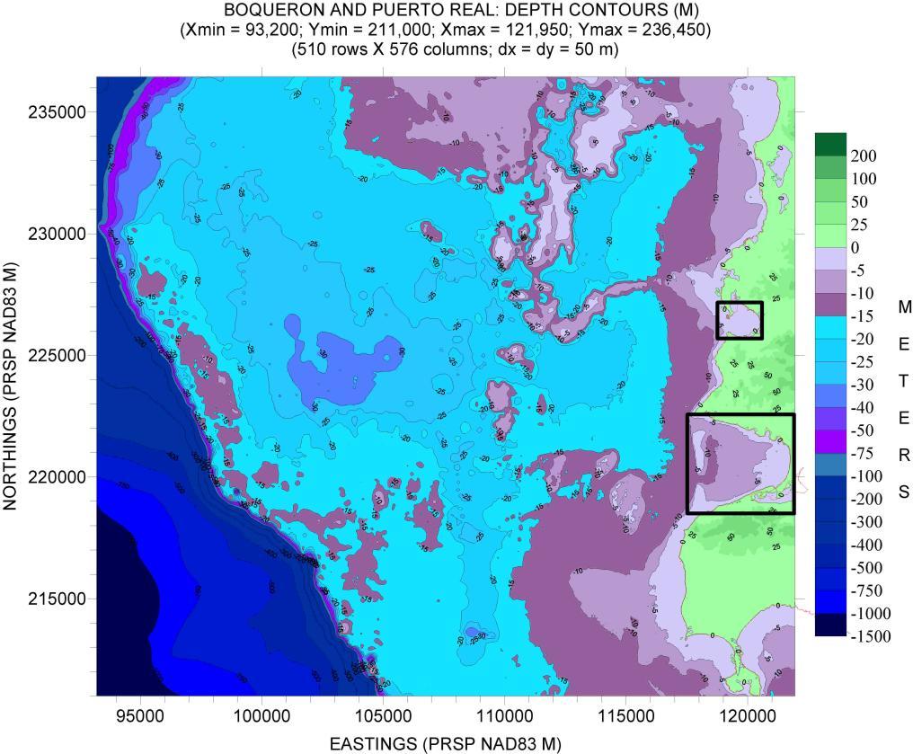
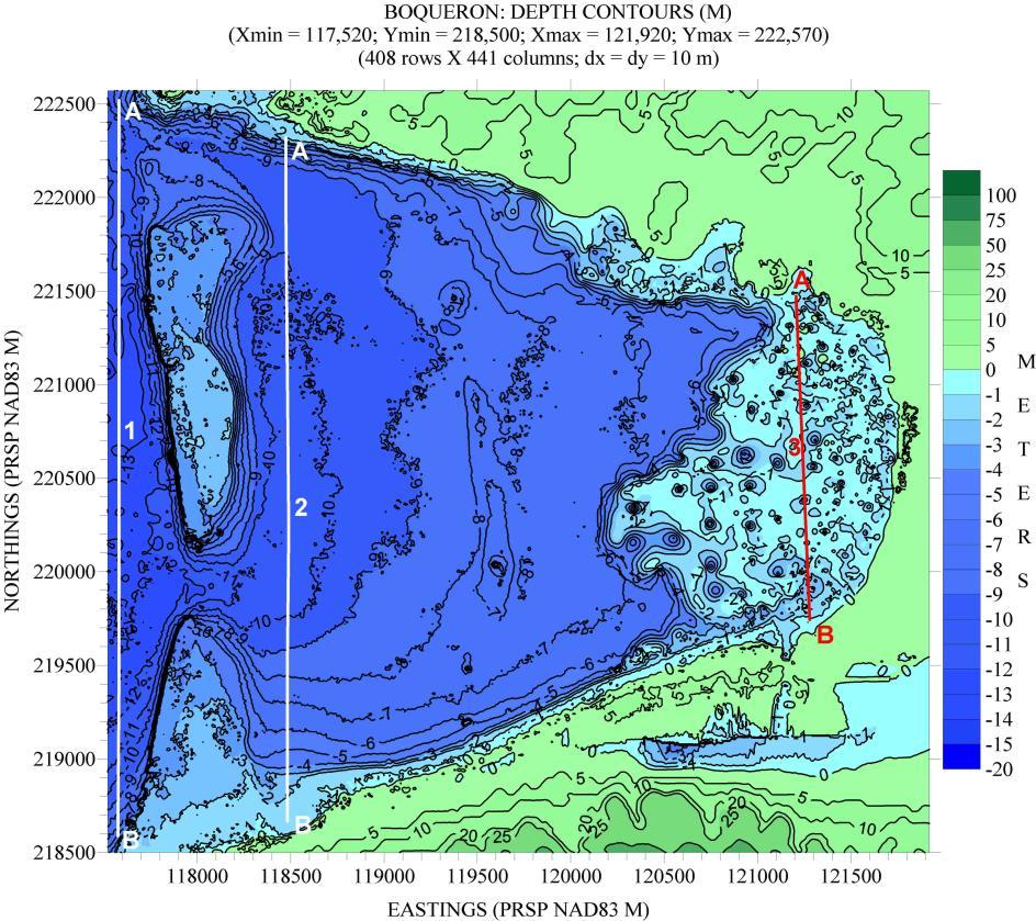
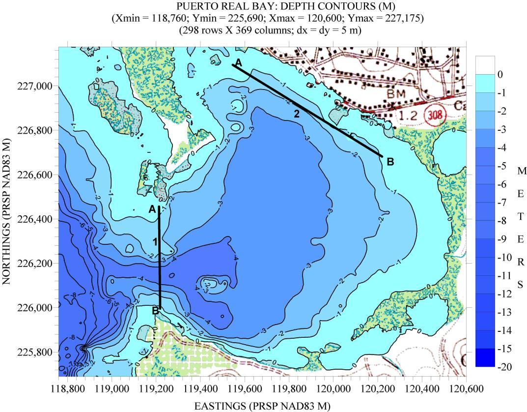
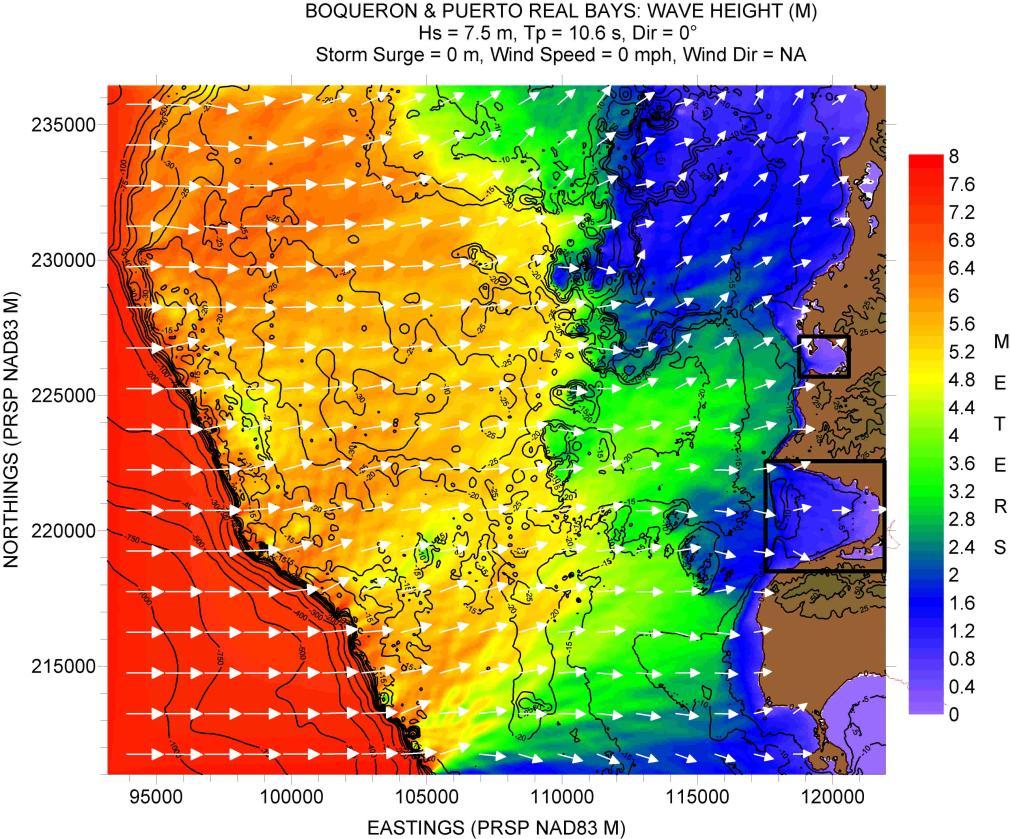
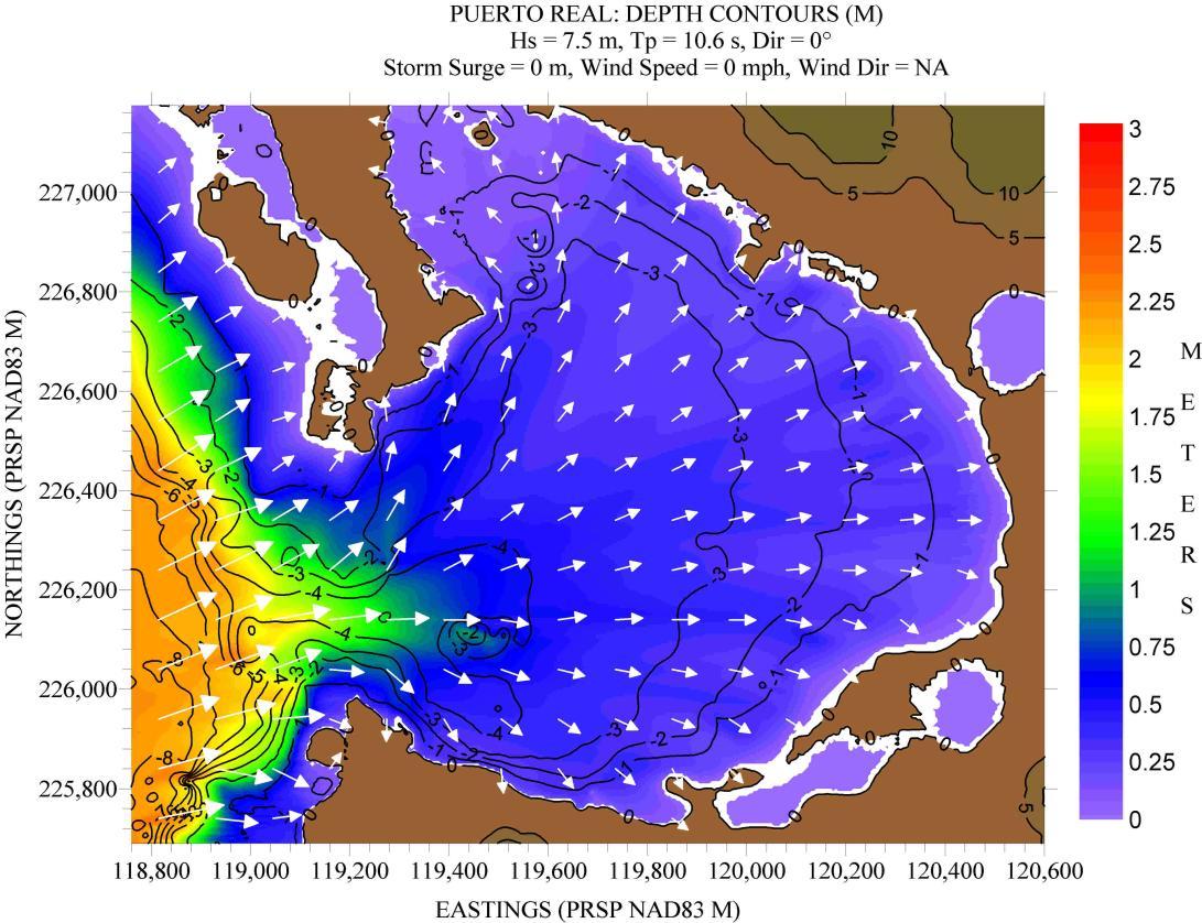
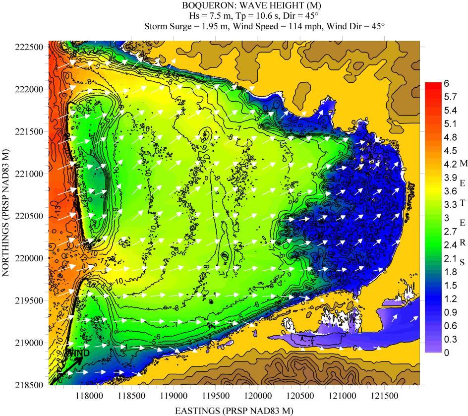
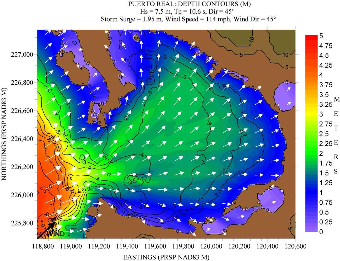
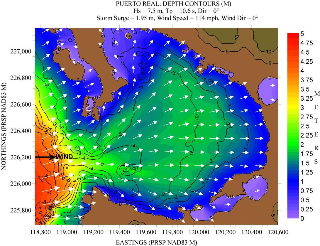
Figure 126 shows the locations where bathymetry and topography values are available. Figure 127 shows a depth contour plot of the computational grid for this location. It also shows the outline of the two nested grids used: Boquerón Bay and Puerto Real. Figures 128 and 129 show depth contour plots for the two nested computational grids. Both figures show the locations of the slices to be taken.
It should be mentioned that inside Boquerón Bay there are problems with the bathymetry coverage. This is reflected in the strange depth contours seen along the eastern side of the bay in Figure 128. This is due to the fact that the SHOALS coverage left gaps inside the bay that I tried to fill in with much older (circa 1904) NOS data. Apparently there is a discontinuity in the z values that leads to the peculiar contour patterns seen in the figure. Hence, the Hs values along the transect (or slice) shown in this part of the bay (#3) should be taken with caution.
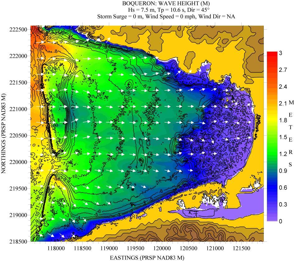
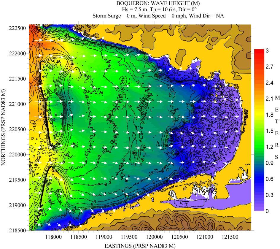
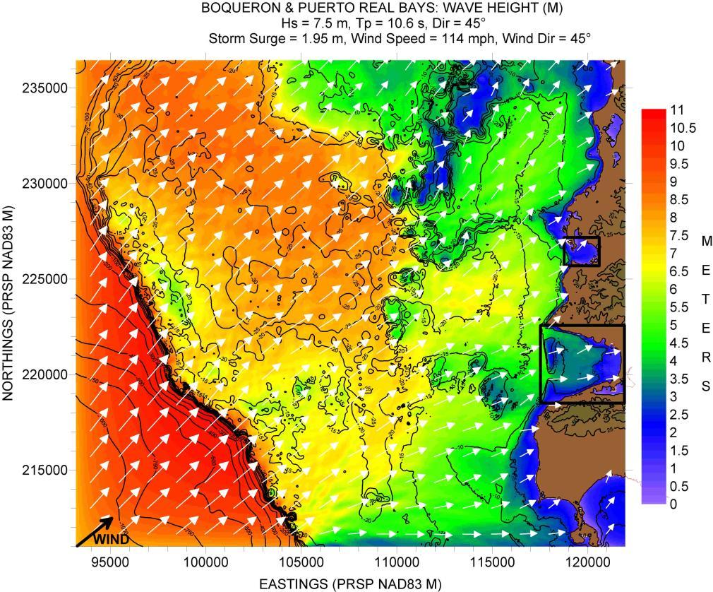
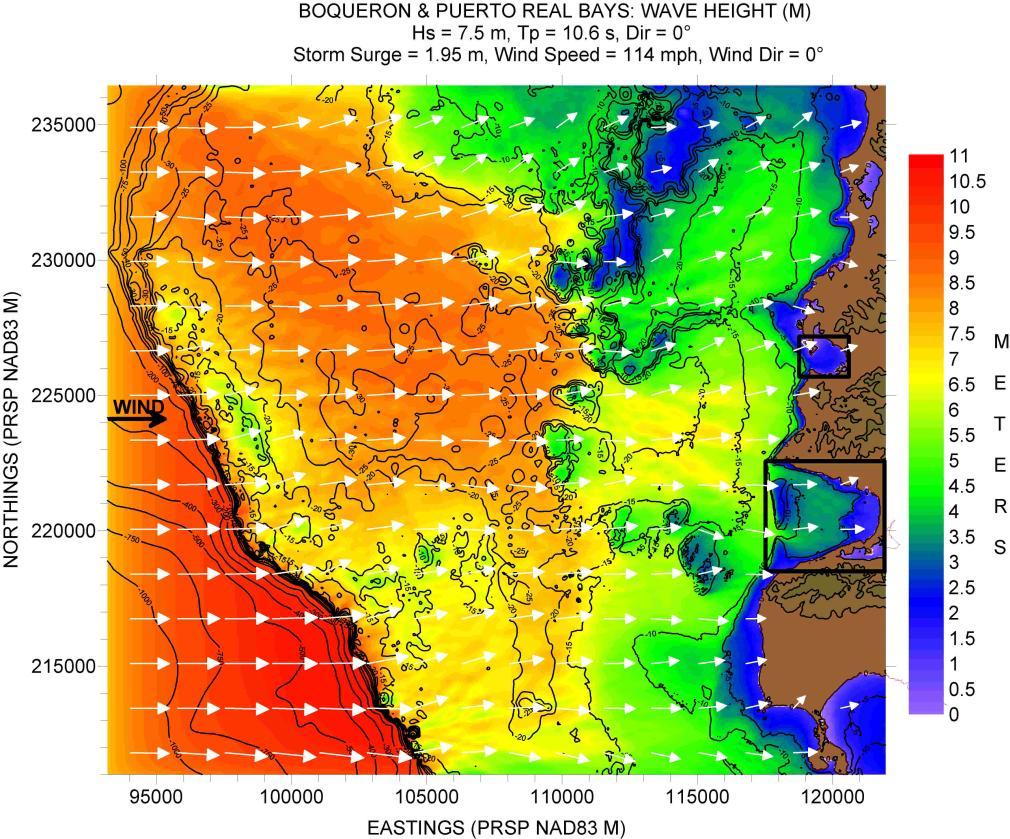
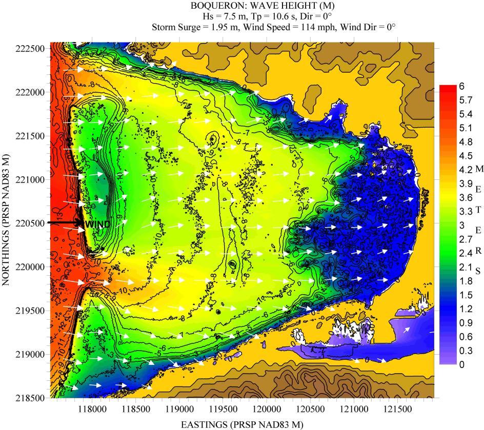
This location has, together with the east coast, the peculiarity of a wide island shelf, forcing the outer computational grid to extend approximately 25 km east-west and north-south. Figures 130 to 141 show the results for the scenarios listed along the top margin of the figures. Two wave directions were considered: 1) waves propagating from the southwest and, 2) waves propagating from the west.
Boquerón Bay:
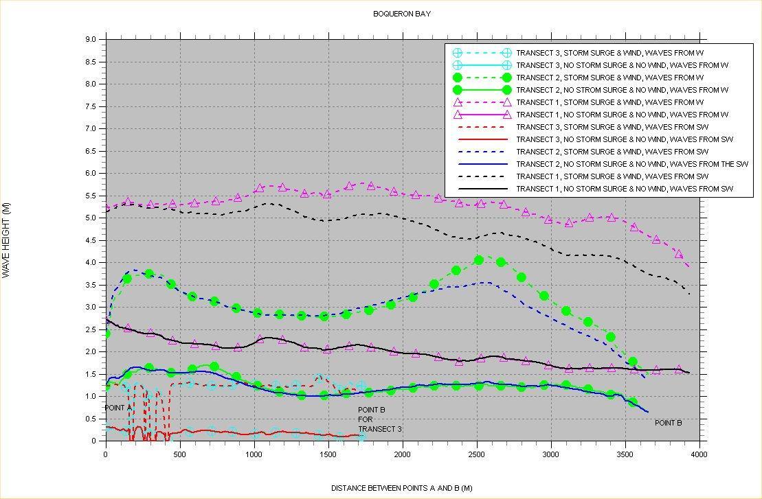
The entrance to this bay is somewhat protected by shallow depths, leaving an entrance channel along the north side of the bay and a slightly deeper south of it. The results (see Figure 142) show that there is not much difference between the two offshore wave directions. Results for Transect 1 (just outside the bay) show that waves 2 to 2.5 m can reach the bay entrance under no storm surge and no wind conditions. This is increased to 4 to 5.5 m under storm surge and wind conditions (decreasing from north to south) Once inside the bay (Transect 2) the values under no storm surge and no wind conditions decrease to 1 – 1.5 m, increasing to 2.5 – 4 m under storm surge and wind conditions (with peaks in the variability along the “slices” corresponding to where the two entrance channels lie). For the easternmost transect (#3) results vary from less than 0.5 m under no storm surge and no wind conditions, up to 1 – 1.5 m under both conditions. But remember the caveat about the bathymetry in the region where Transect 3 is located. In general, the western half of the bay can be impacted by waves higher than 3 m under extreme conditions.
Puerto Real:
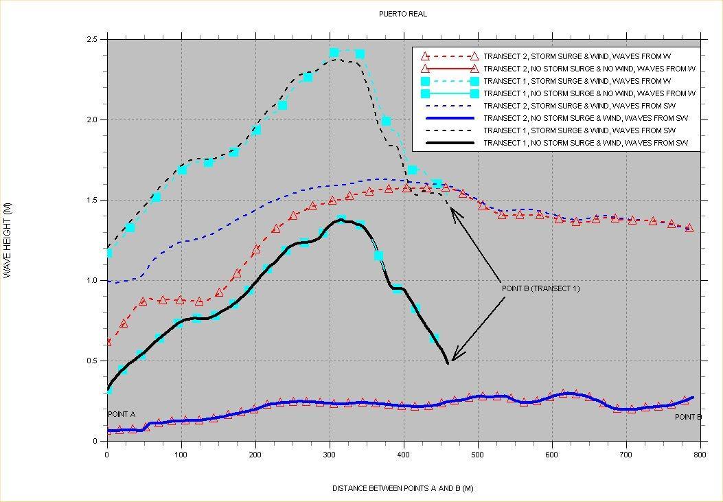
Figure 143 shows that results do not differ much between the two deepwater wave directions used. As a matter of fact, results for Transect 1 and 2 are the same for the case of no storm surge and no wind. It is only under storm surge and wind forcing that they differ, but not much. It can be seen that the Puerto Real village is well protected from waves even under storm conditions.
126. Posting showing location of bathymetry and topography values for Boquerón Bay and Puerto Real.
127. Depth contour plot of outer computational grid for Boquerón Bay and Puerto Real. Also shown is the outline of nested grids.
Figure
Figure
Figure 128. Depth contour plot of nested computational grid for Boquerón Bay.
Figure 129. Depth contour plot of nested computational grid for Puerto Real Bay.
Figure 130. Hs contour plot for Boquerón and Puerto Real Bays, based on the scenario listed along the top margin of figure.
Figure 131. Hs contour plot for (nested) Boquerón, based on the scenario listed along the top margin of figure.
Figure 132. Hs contour plot for (nested) Puerto Real, based on the scenario listed along the top margin of figure.
Figure 133. Hs contour plot for Boquerón and Puerto Real Bays, based on the scenario listed along the top margin of figure.
Figure 134. Hs contour plot for (nested) Boquerón, based on the scenario listed along the top margin of figure.
Figure 135. Hs contour plot for (nested) Puerto Real, based on the scenario listed along the top margin of figure.
Figure 136. Hs contour plot for Boquerón and Puerto Real Bays, based on the scenario listed along the top margin of figure.
Figure 137. Hs contour plot for (nested) Boquerón, based on the scenario listed along the top margin of figure.
Figure 138. Hs contour plot for (nested) Puerto Real, based on the scenario listed along the top margin of figure.
Figure 139. Hs contour plot for Boquerón and Puerto Real Bays, based on the scenario listed along the top margin of figure.
Figure 140. Hs contour plot for (nested) Boquerón, based on the scenario listed along the top margin of figure.
Figure 14100219. Hs contour plot for (nested) Puerto Real, based on the scenario listed along the top margin of figure.
Figure 142. Significant wave height “slices” for Boquerón Bay.
Figure 143. Significant wave height “slices” for Puerto Real.
MAYAGUEZ
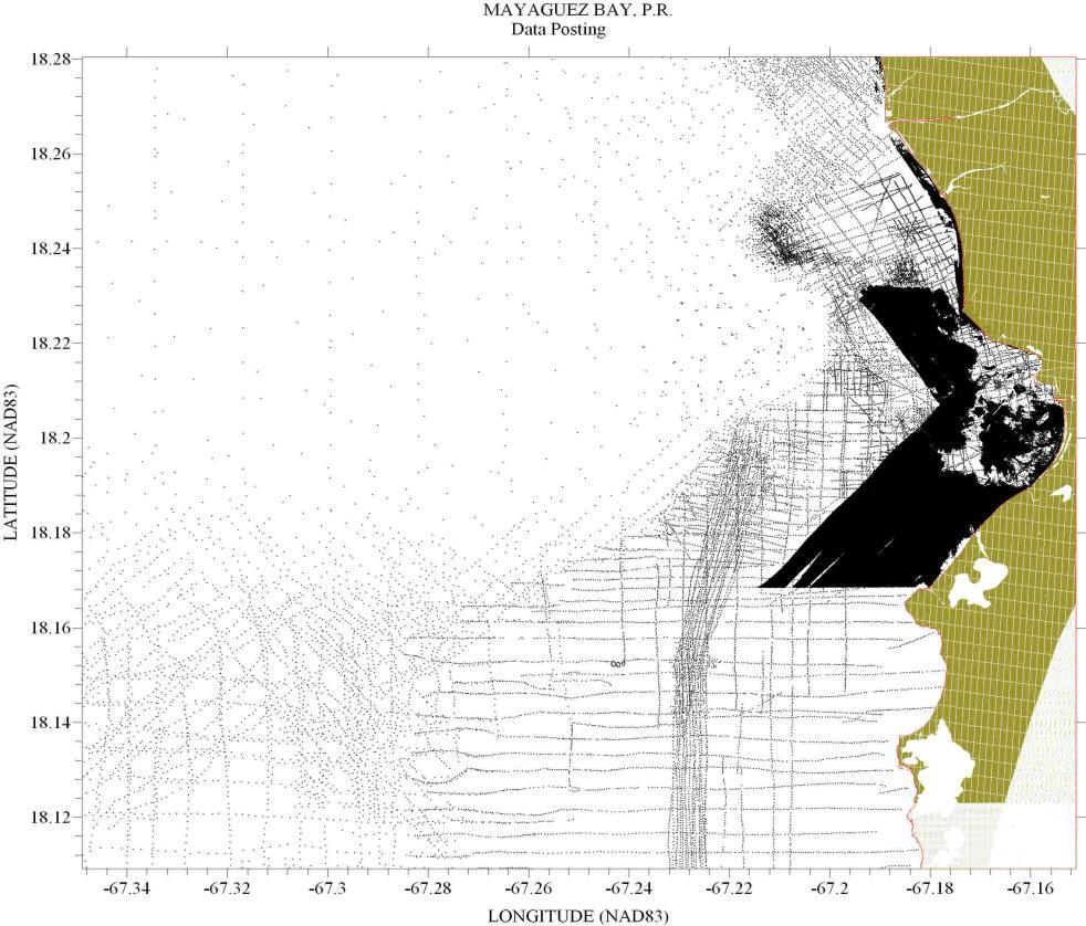
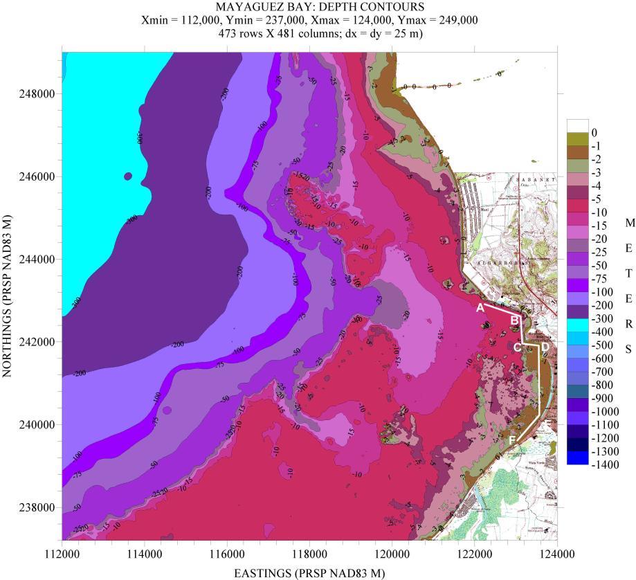
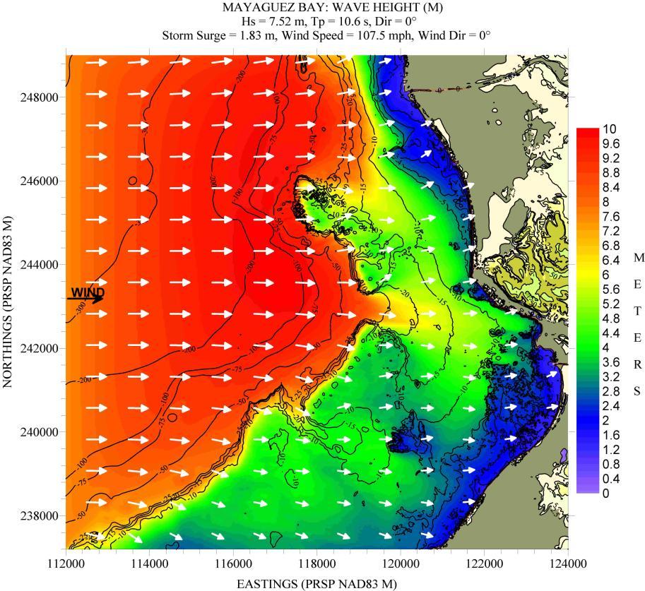
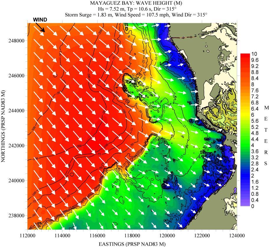
Figure 144 shows the location of the bathymetry and topography values, while Figure 145 shows a depth contour plot of the computational grid. This figure shows the “slice” along which Hs values will be taken. Results are shown in Figures 146 to 149. Two offshore wave directions were considered: waves from the west and from the northwest.
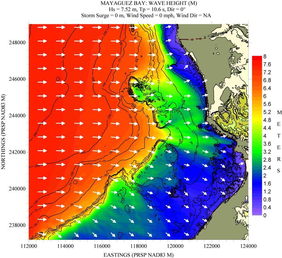
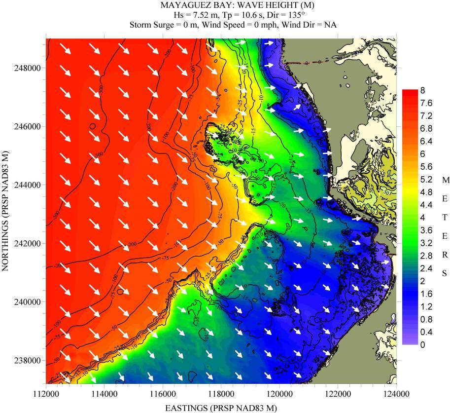
This bay is another example where the entrance channel facilitates wave energy penetration into the northern half of the bay. And the shelf break lies close to the coastline. But once near shore, the wave height is determined by the water depth. In deeper waters inside the bay, Hs values between 3 to 4 m in height can be seen in the figures along the northern part of the bay under no storm surge and wind conditions. Once storm surge and wind conditions are included then these values are increased to 4 to 6 m. These conditions are specifically seen north of the Yaguez River mouth.
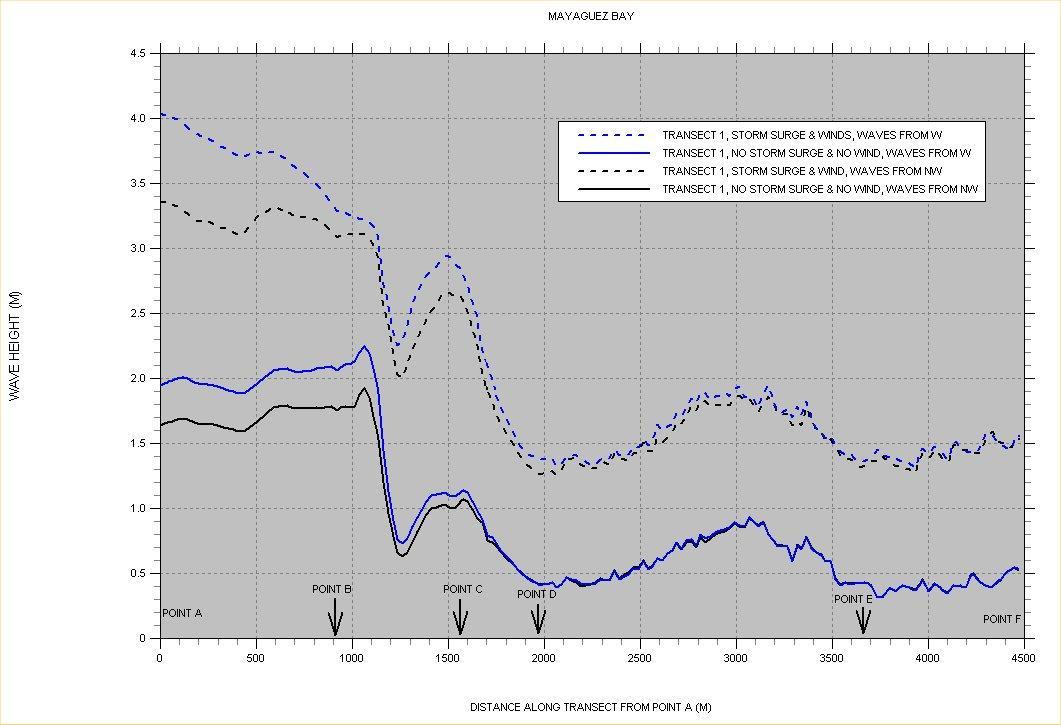
Figure 150 shows the variation of Hs along the “slice” shown in Figure 145. We should remember the caveat that, since we are in shallow water, most of this variability reflects depth variations along the “slice”. The figure corroborates the statement that it is the northern part of the bay which is most exposed, with Hs values varying between 1.5-2 m for the no storm surge and no wind condition, up to 3.5-4 m for the storm condition.
144. Posting showing location of bathymetry and topography values for Mayaguez Bay.
Figure
Figure 145. Depth contour plot of computational grid for Mayagüez Bay.
Figure 146. Hs contour plot for Mayaguez Bay, based on the scenario listed along the top margin of figure.
Figure 147. Hs contour plot for Mayaguez Bay, based on the scenario listed along the top margin of figure.
Figure 148. Hs contour plot for Mayaguez Bay, based on the scenario listed along the top margin of figure.
Figure 149. Hs contour plot for Mayaguez Bay, based on the scenario listed along the top margin of figure.
Figure 150. Significant wave height “slices” for Mayaguez Bay.
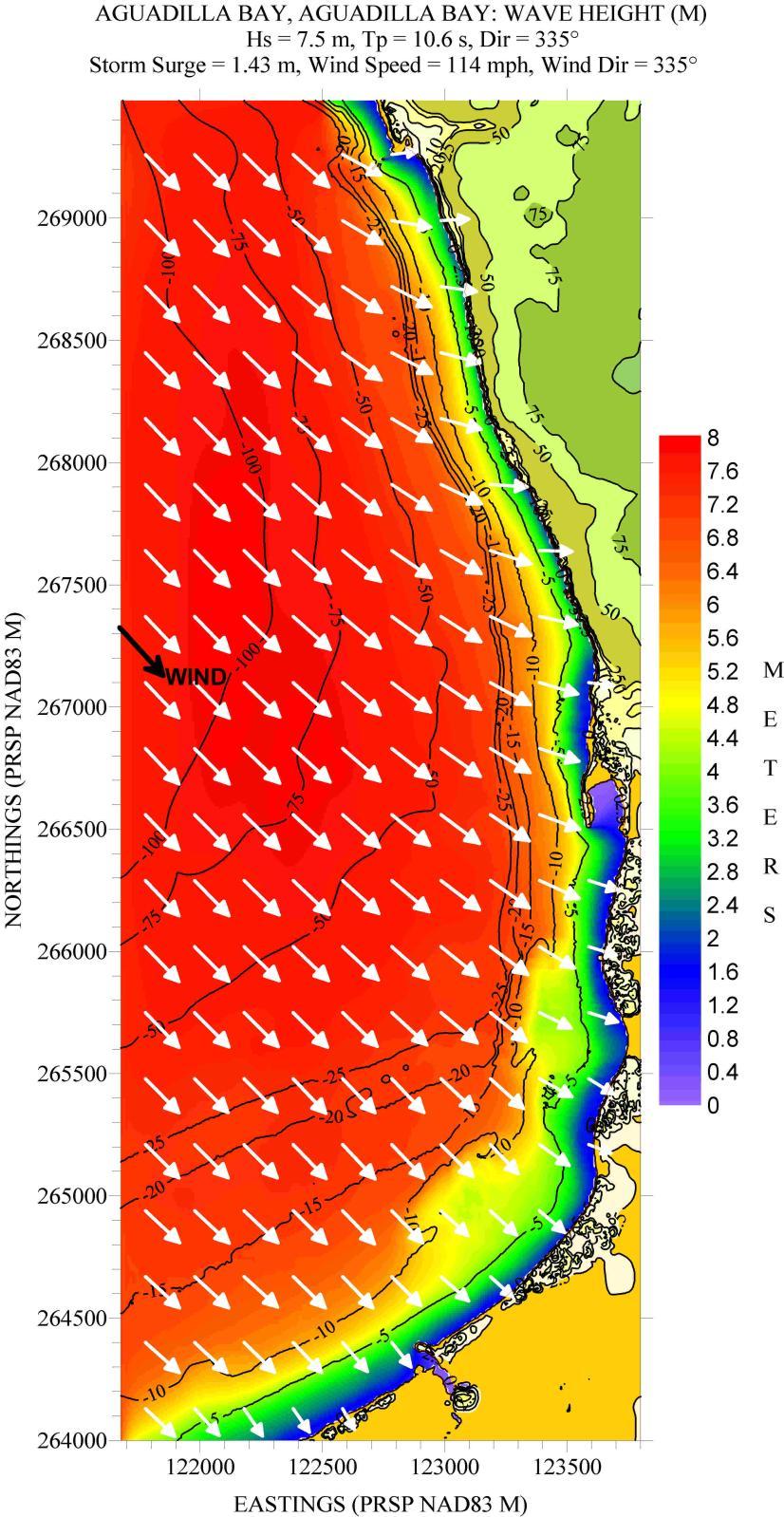
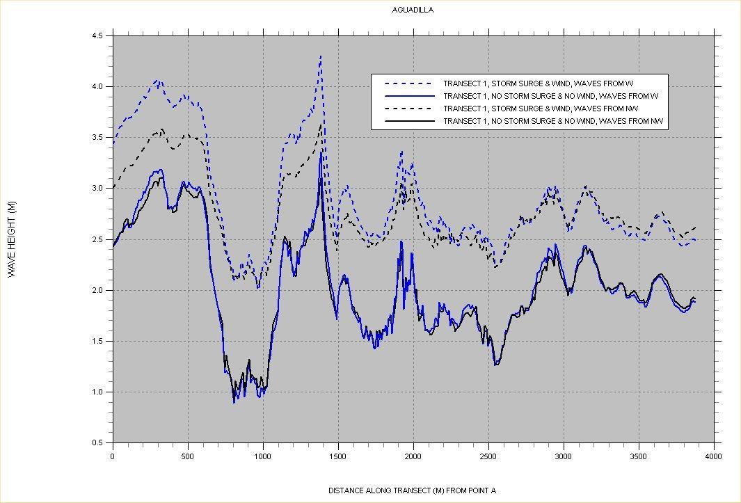
AGUADILLA
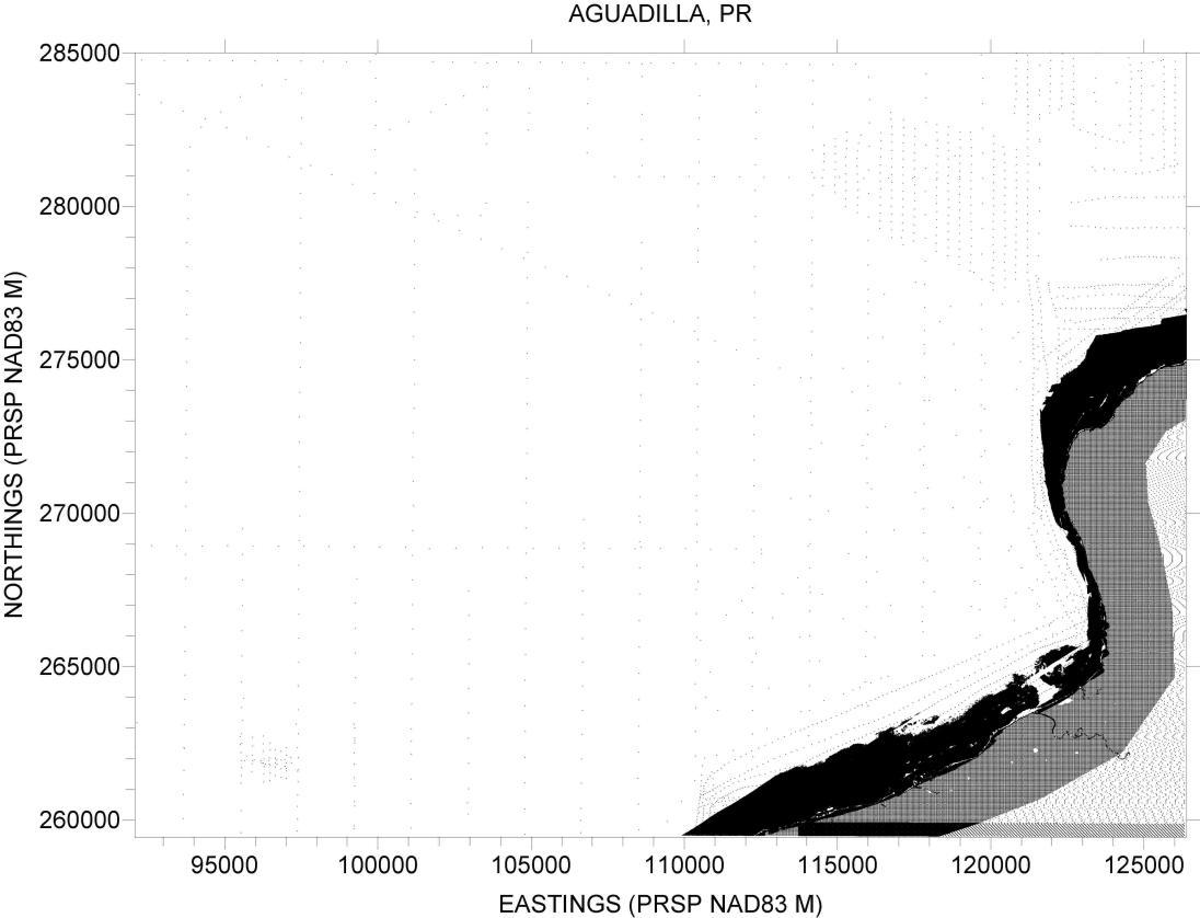
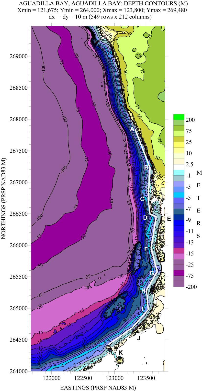
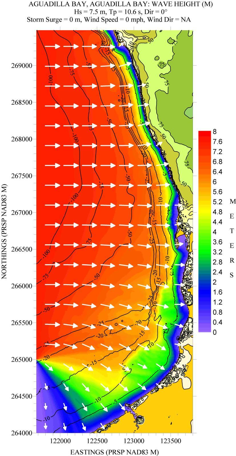
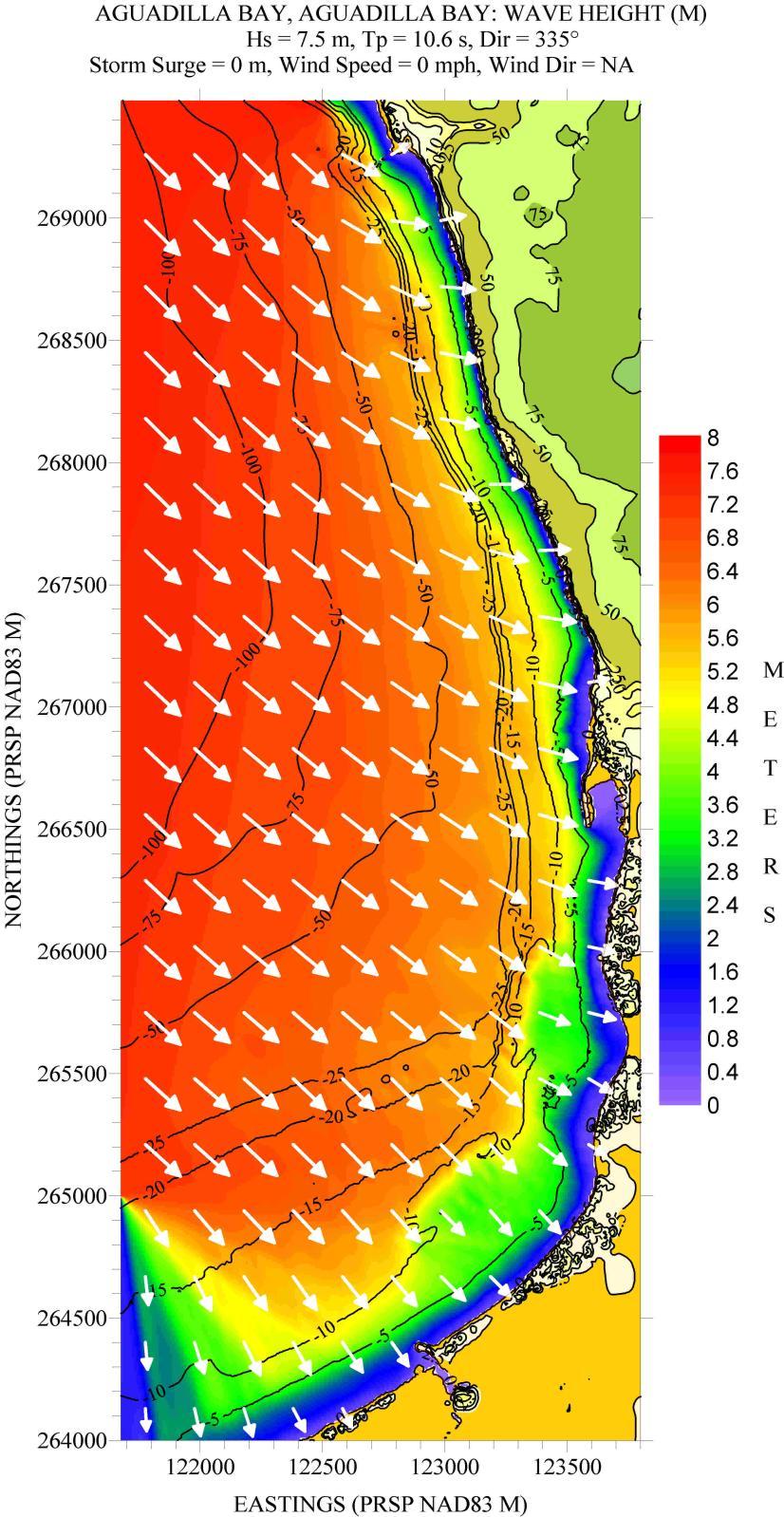
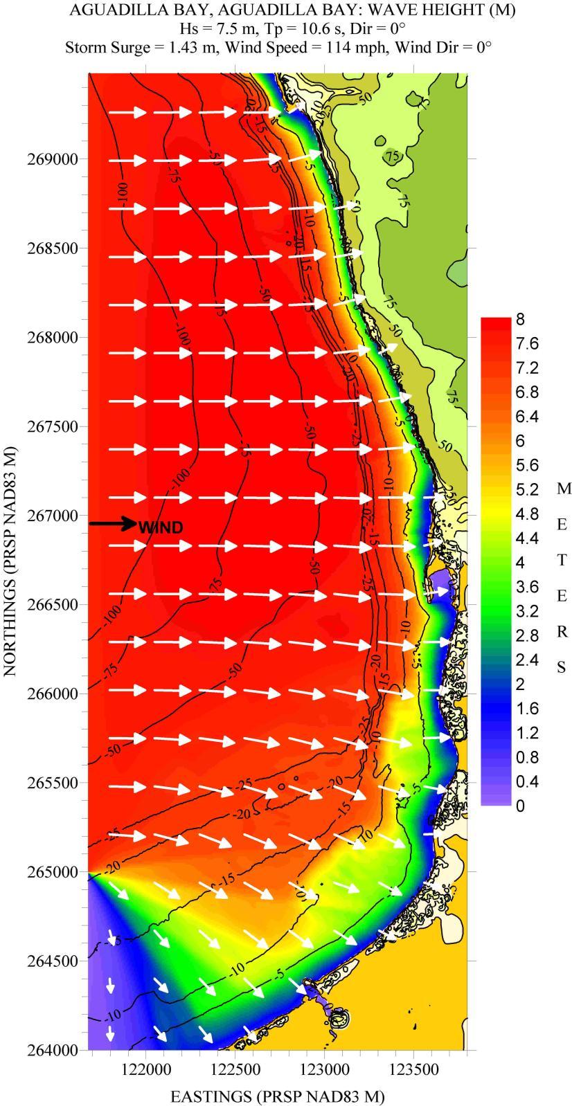
Figure 151 shows the location of bathymetry and topography values used for preparing the computational grid. Figure 152 shows a depth contour plot of the computational grid and the “slice” for obtaining Hs values. Figures153 to 156 show the results for the different scenarios listed along the top margin of each figure. Two deepwater wave directions were considered: waves from the northwest and west. As expected, Aguadilla Bay is well exposed to waves propagating in from a window between north and approximately, west. There is practically no shelf fronting the city, allowing large waves ( 3 m) to break very close to shore
Again, keeping in mind that Hs variations along the “slice” will mainly reflect depth variations, Figure 157 corroborates the above statement about the exposure of the bay. There is not much variation in the results between the two directions considered.
Figure 151. Posting showing location of bathymetry and topography values for Aguadilla Bay.
Figure 152. Depth contour plot of computational grid for Aguadilla Bay.
listed along the top margin of figure.
Figure 153. Hs contour plot for Aguadilla Bay, based on the scenario
listed along the top margin of figure.
Figure 154. Hs contour plot for Aguadilla Bay, based on the scenario
listed along the top margin of figure.
Figure 155. Hs contour plot for Aguadilla Bay, based on the scenario
listed along the top margin of figure.
Figure 156. Hs contour plot for Aguadilla Bay, based on the scenario
Figure 157. Significant wave height “slices” for Aguadilla Bay.
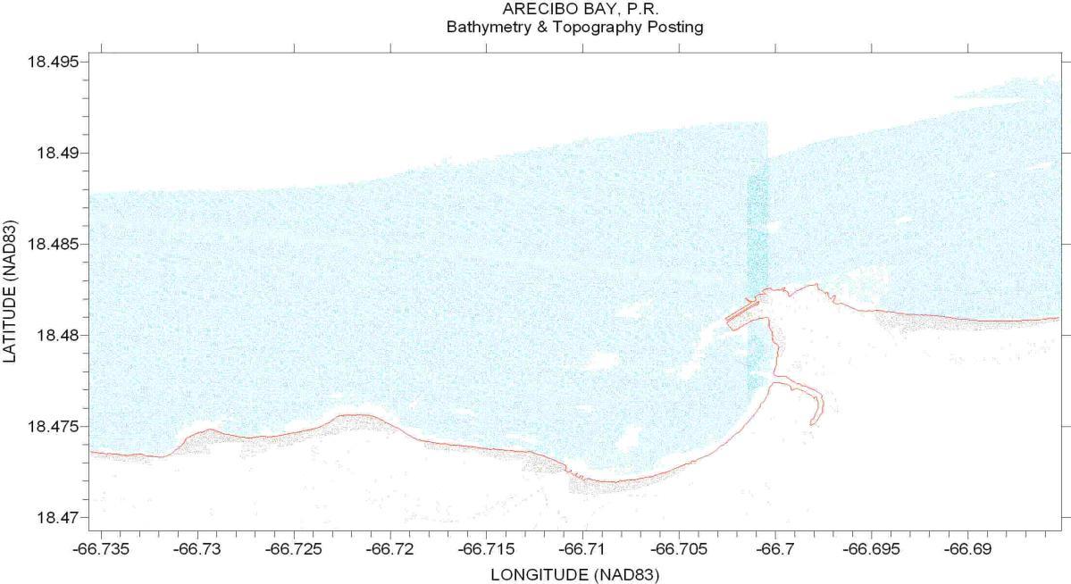
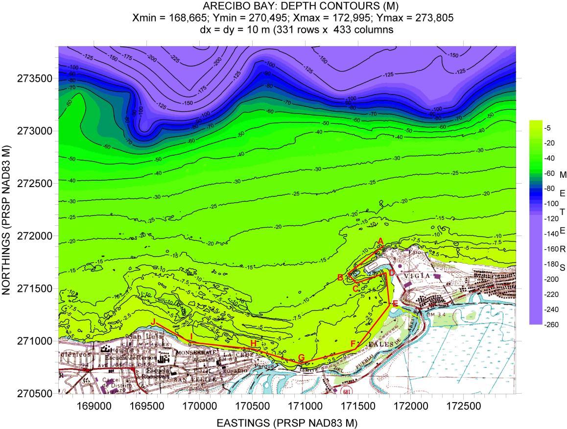
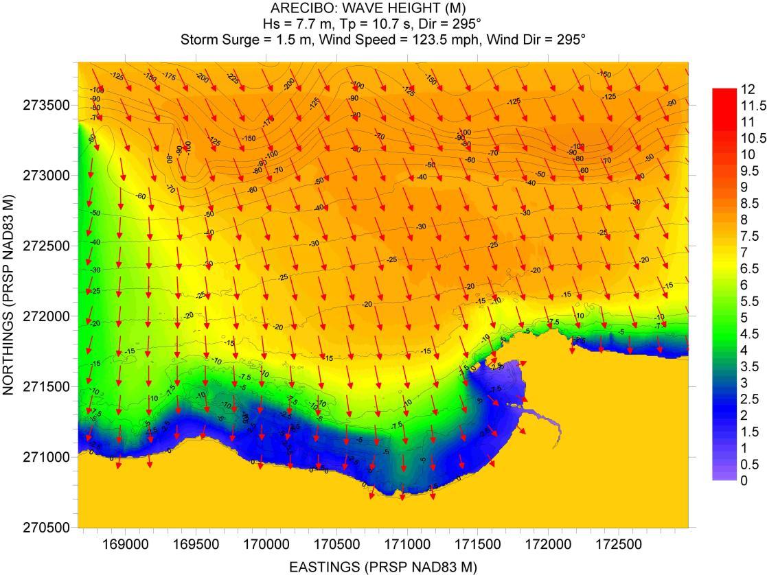
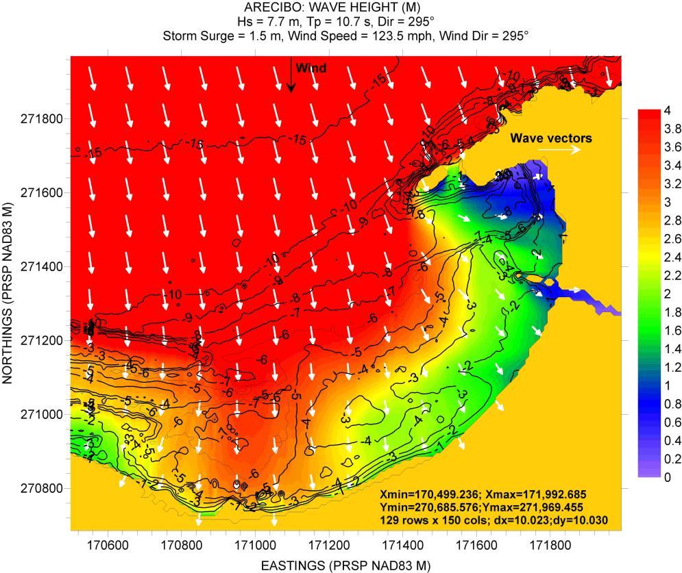
ARECIBO
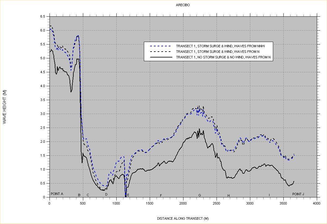
Figure 158 shows the location of the bathymetry and topography values used to prepare the computational grid. Figure 159 shows a depth contour plot of the computational grid.. Two deepwater wave directions were considered: waves from the north and north-northwest. Figures 160 to 165 show the results. This bay is also well exposed to big waves, as expected. Besides having no natural protection and being open to the North Atlantic, it has a very narrow shelf, allowing waves as high to 5 m to crash half a kilometer away, under no storm surge and no wind conditions. What seems to be an ancient Rio Grande de Arecibo mouth allows waves close to 3.25 m in height to crash practically against the coast Figure 166 corroborates this. The best protected section lies between transect sections D-E-F, at the eastern side of the bay.
158. Posting showing location of bathymetry and topography values for Arecibo Bay.
computational
Figure
Figure 159. Depth contour plot of
grid for Arecibo Bay.
Figure 160. Hs contour plot for Arecibo Bay, based on the scenario listed along the top margin of figure.
Figure 161. Hs contour plot for Arecibo Bay, based on the scenario listed along the top margin of figure.
Figure 162. Hs contour plot for Arecibo Bay, based on the scenario listed along the top margin of figure.
Figure 163. Hs contour plot for Arecibo Bay, based on the scenario listed along the top margin of figure.
Figure 164. Hs contour plot for Arecibo Bay, based on the scenario listed along the top margin of figure.
Figure 165. Hs contour plot for Arecibo Bay, based on the scenario listed along the top margin of figure.
Figure 166. Significant wave height “slices” for Arecibo Bay.
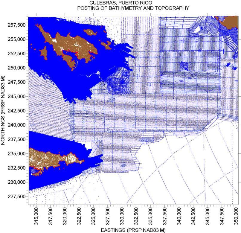
CULEBRA, ENSENADA HONDA
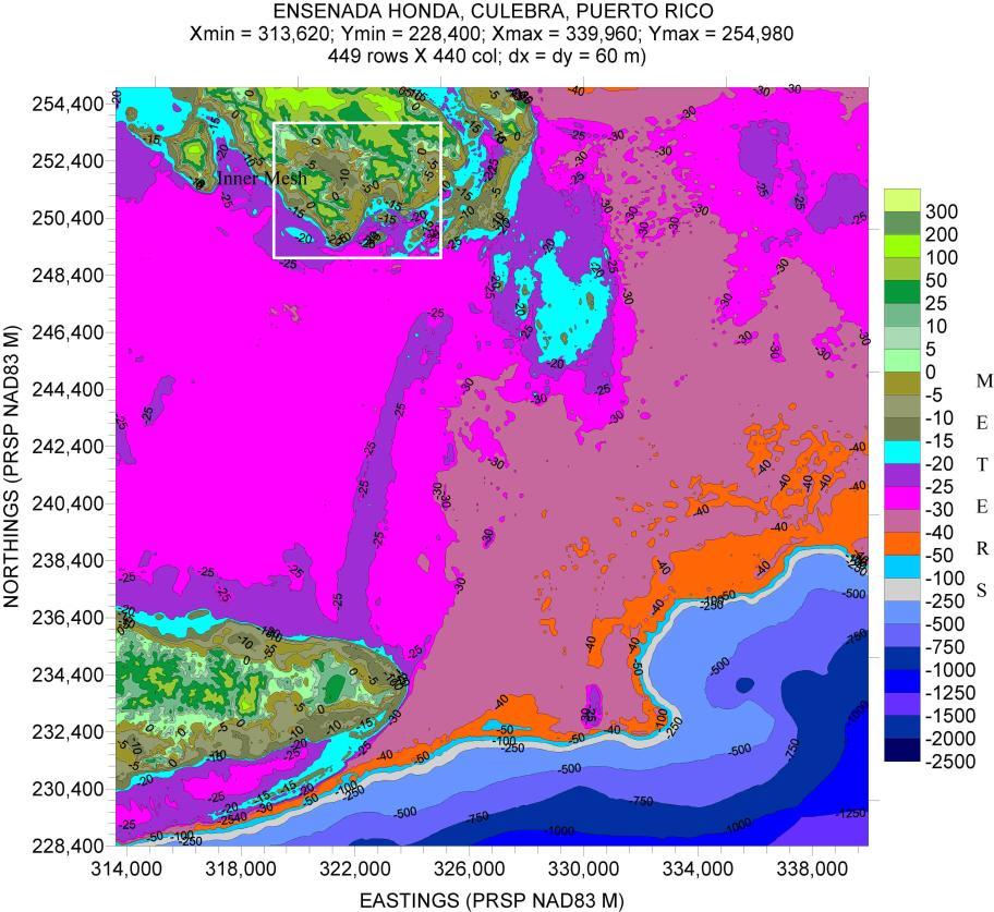
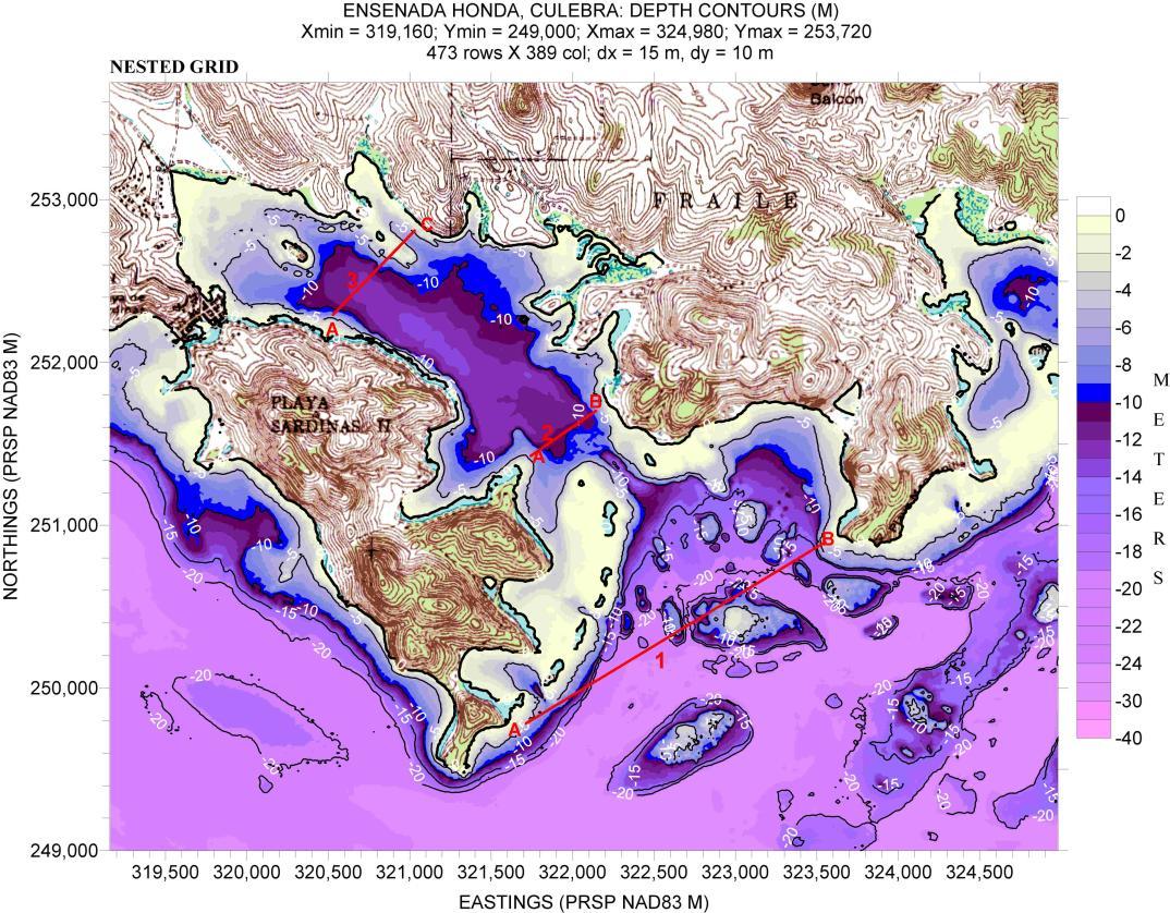
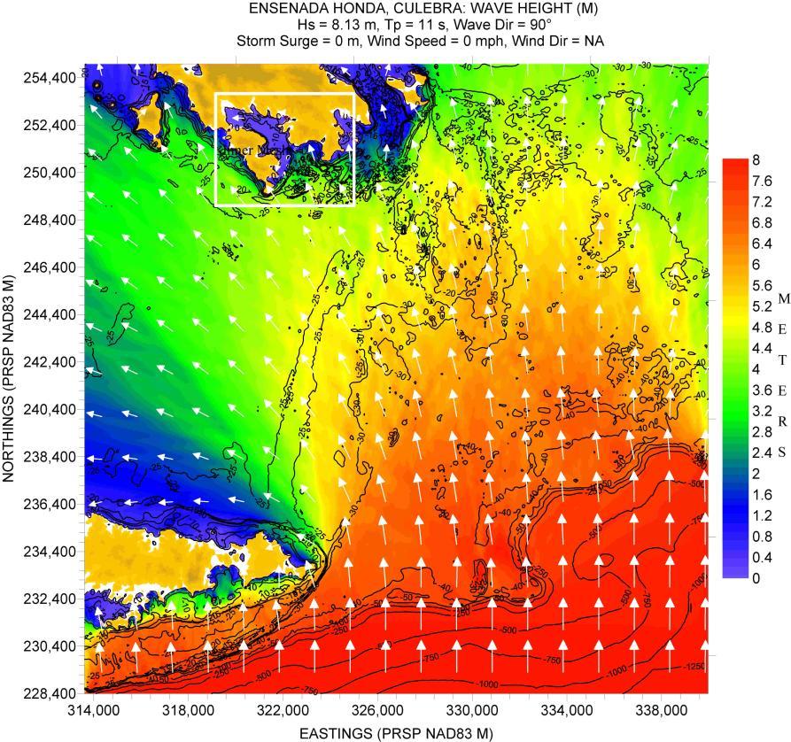
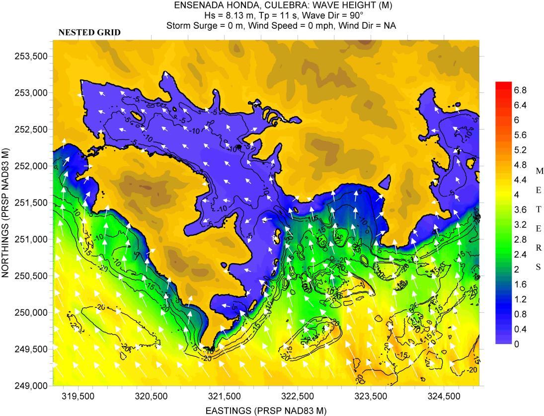
Figure 167 shows a posting of the bathymetry and topography locations used in the preparation of the outer and nested computational grids shown in Figures 168 and 169, respectively. Figure 169 shows the locations for the Hs “slices”. A large outer grid is required because of the extensive shelf east of Puerto Rico. Two deepwater wave directions were simulated: from the southeast and south.
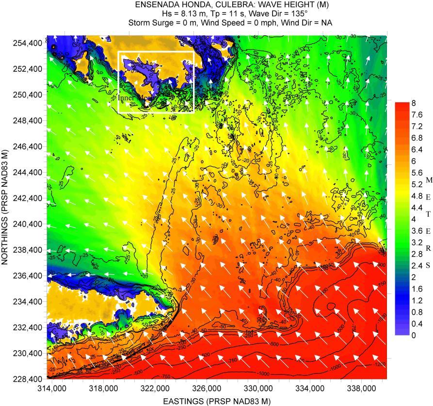
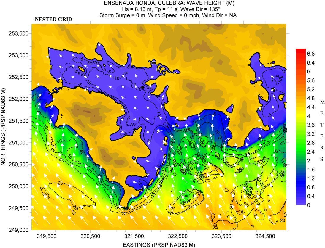
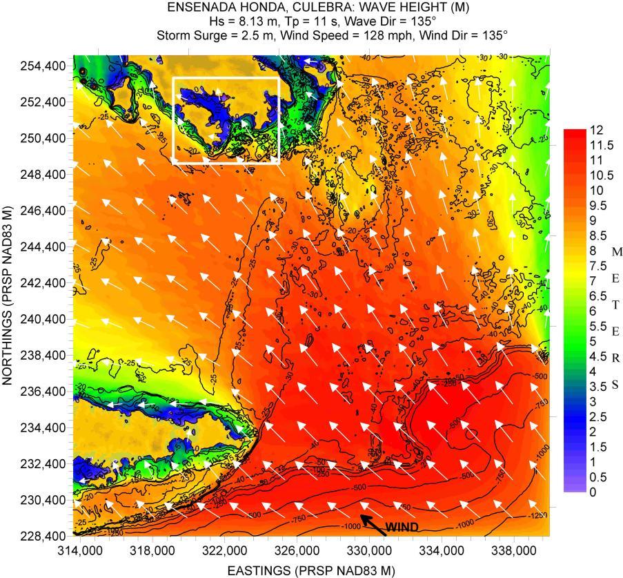
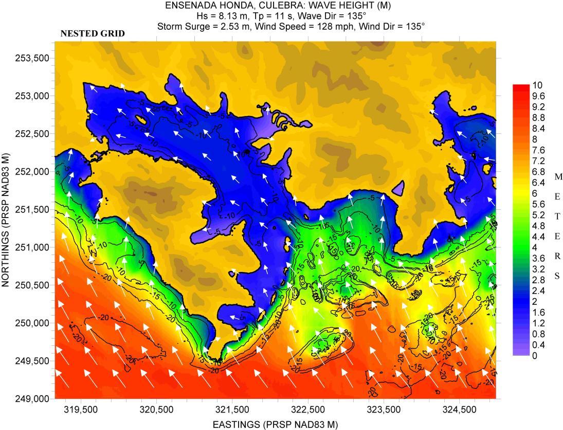
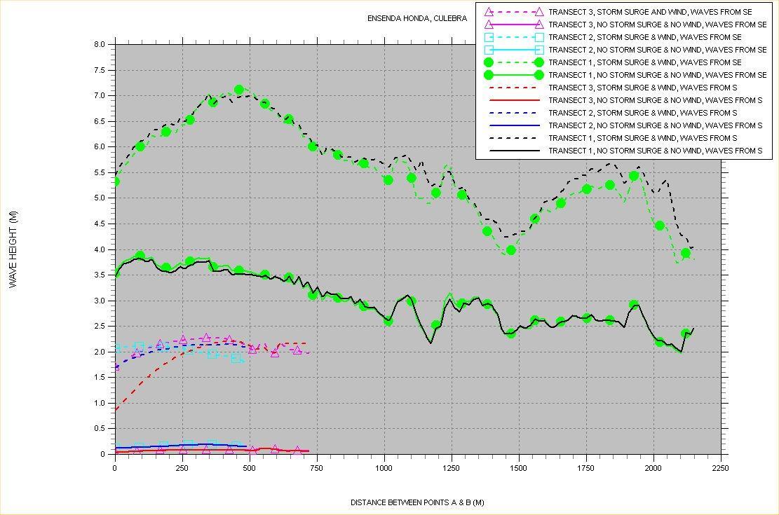
Figures 170 to 177 show contour plots for the Hs results. This bay is also very well protected from wave attack due to its very narrow, and relatively long, entrance channel, protected by fringing reefs. The figures show how the big waves are stopped right at the entrance to the channel. All of this is corroborated by Figure 178, showing the Hs variation at three different locations along the bay. Even under storm surge and wind conditions, Hs heights inside the bay are not higher than approximately 2 m. The fact that results are practically the same at Transects 2 and 3 seems to imply that wave growth inside the bay between these two transects, under these very strong wind conditions, is happening.
This conclusion about how well protected this bay is regarding wave action, when compared with the destruction brought about by Hurricane Hugo in 1989, where all types of boats and yachts could be seen scattered all along the shoreline surrounding the bay, implies that this havoc was due to the combination of storm surge and wind forcing making these to break loose of their moorings, not due to heavy wave action.
167. Posting showing location of bathymetry and topography values for Ensenada Honda Bay, Culebra.
168. Depth contour plot of outer computational grid for Ensenada Honda, Culebra. Also shown is the outline of nested grid.
Figure
Figure
margin of figure.
Figure 169. Depth contour plot of nested computational grid for Ensenada Honda, Culebra.
Figure 170. Hs contour plot for Ensenada Honda, Culebra, based on the scenario listed along the top
Figure 171. Hs contour plot for (nested) Ensenada Honda, Culebra, based on the scenario listed along the top margin of figure.
Figure 172. Hs contour plot for Ensenada Honda, Culebra, based on the scenario listed along the top margin of figure.
Figure 173. Hs contour plot for (nested) Ensenada Honda, Culebra, based on the scenario listed along the top margin of figure.
Figure 174. Hs contour plot for Ensenada Honda, Culebra, based on the scenario listed along the top margin of figure.
Figure 175. Hs contour plot for (nested) Ensenada Honda, Culebra, based on the scenario listed along the top margin of figure.
Figure 176. Hs contour plot for Ensenada Honda, Culebra, based on the scenario listed along the top margin of figure.
the scenario listed along the top margin of figure.
Figure 177. Hs contour plot for (nested) Ensenada Honda, Culebra, based on
Figure 178. Significant wave height “slices” for Ensenada Honda, Culebra.
CHARLOTTE AMALIE, ST. THOMAS, USVI
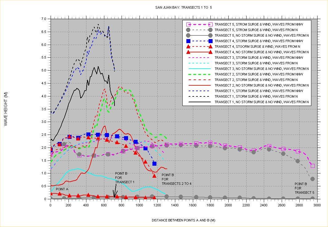
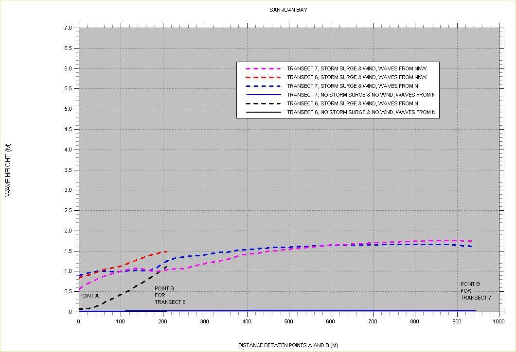
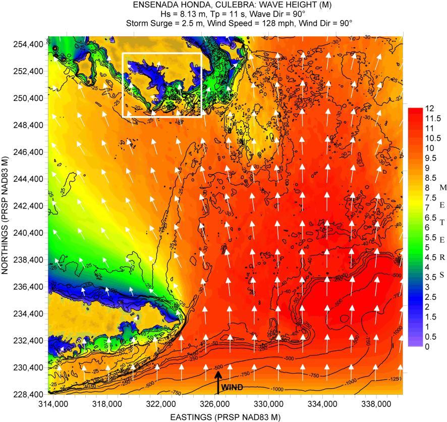
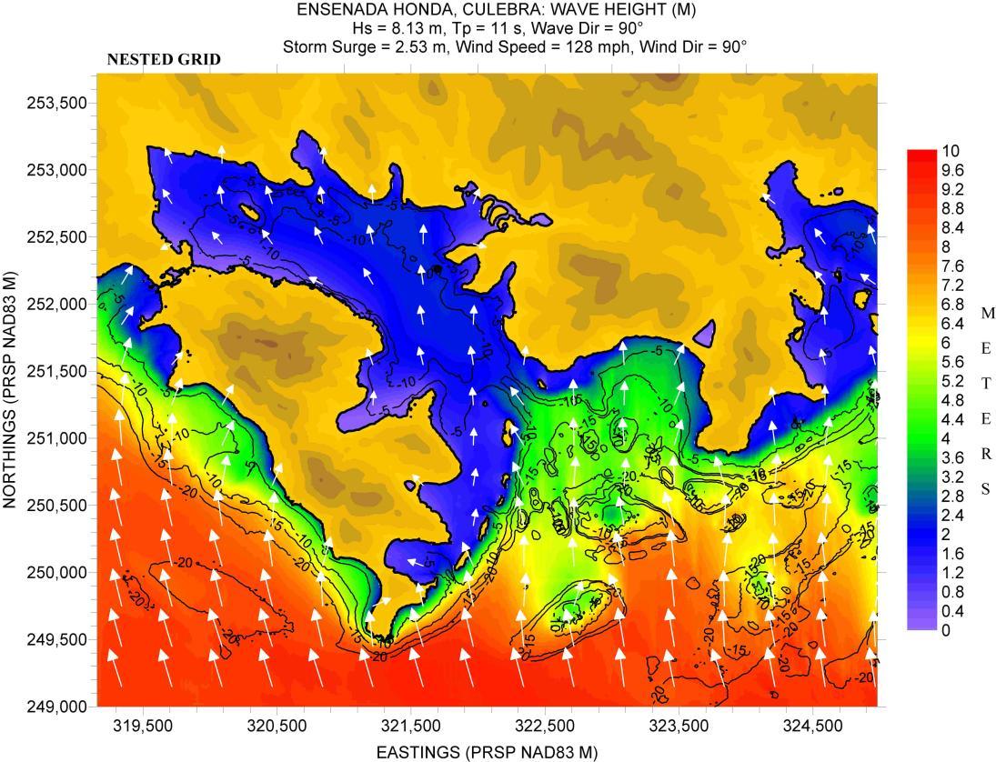
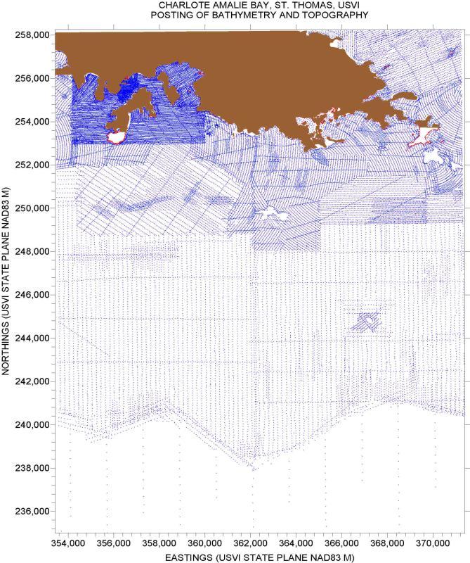
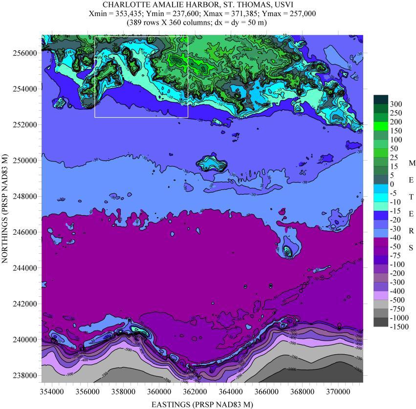
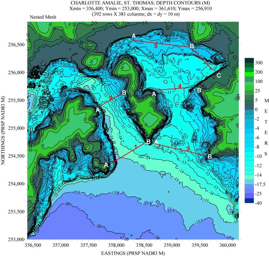
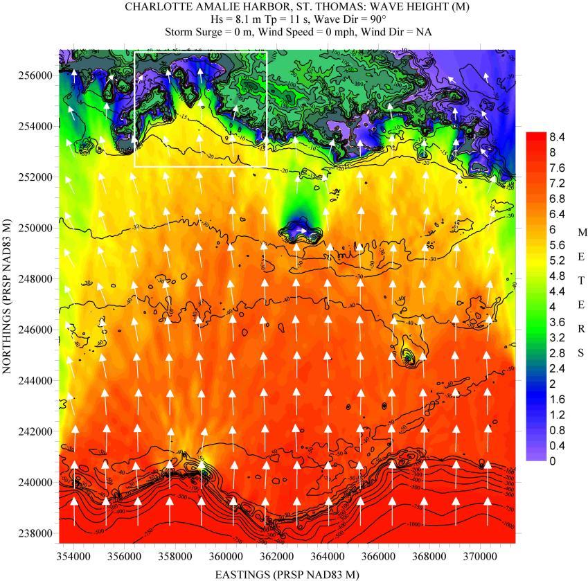
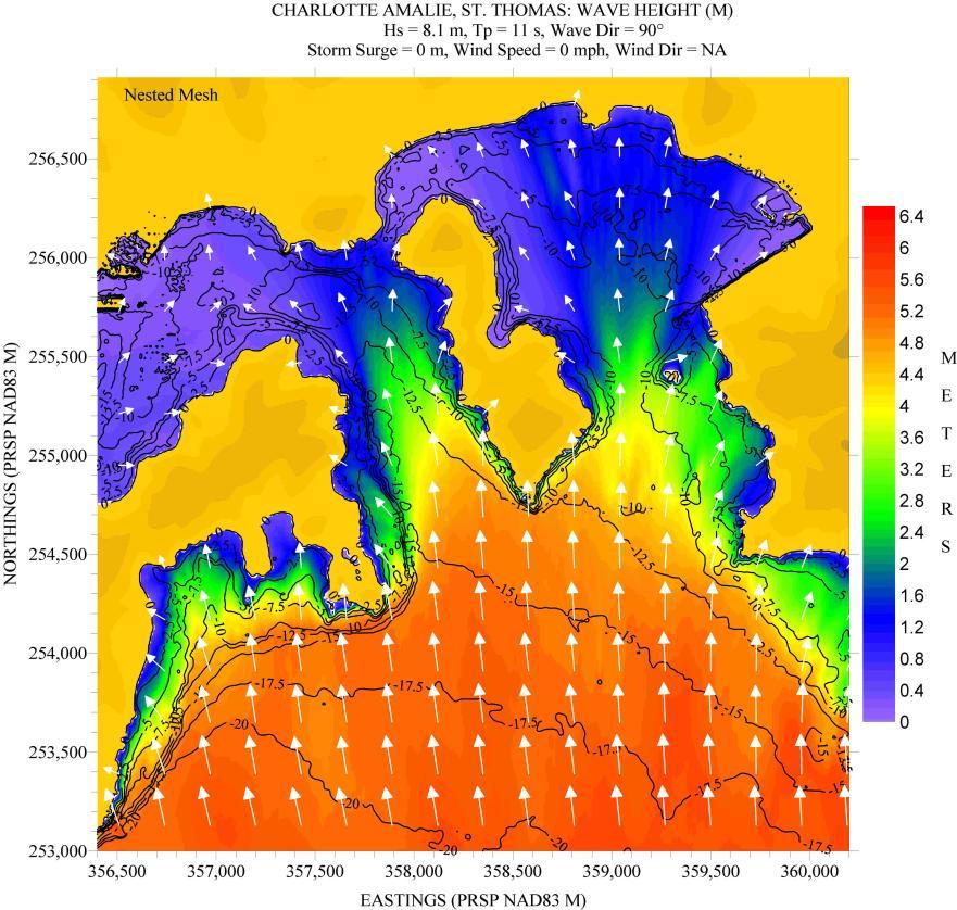
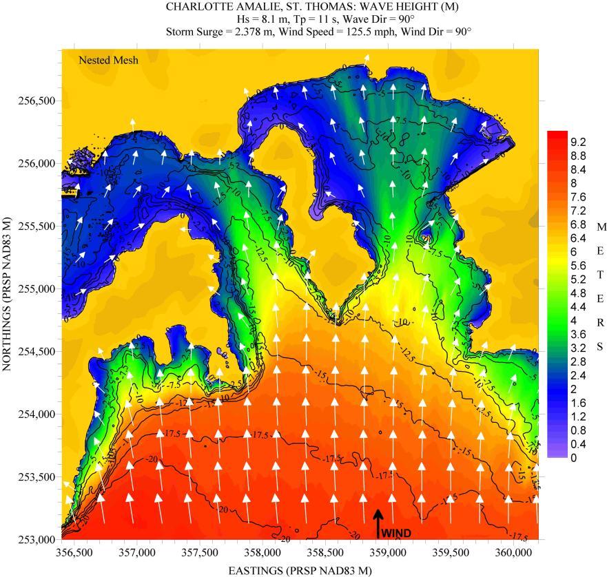
Figure 179 shows the locations where bathymetry and topography values are available. Figure 180 shows a depth contour plot of the outer computational grid, and an outline of the nested grid. Figure 181 shows a depth contour of the nested computational grid, with five transects for the Hs “slices”. Transects 1 and 2 are across East Gregerie Channel (west of Hassel Island, which is the island dividing the bay in two) and Transects 3 to 5 are east of the island.
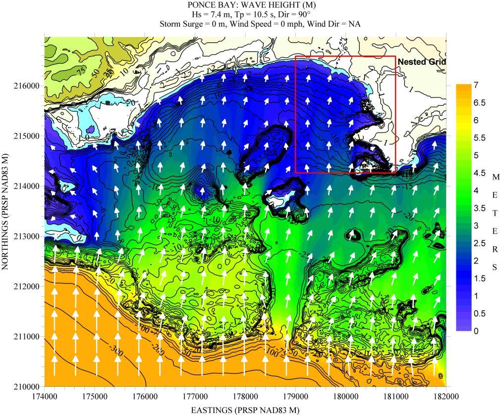
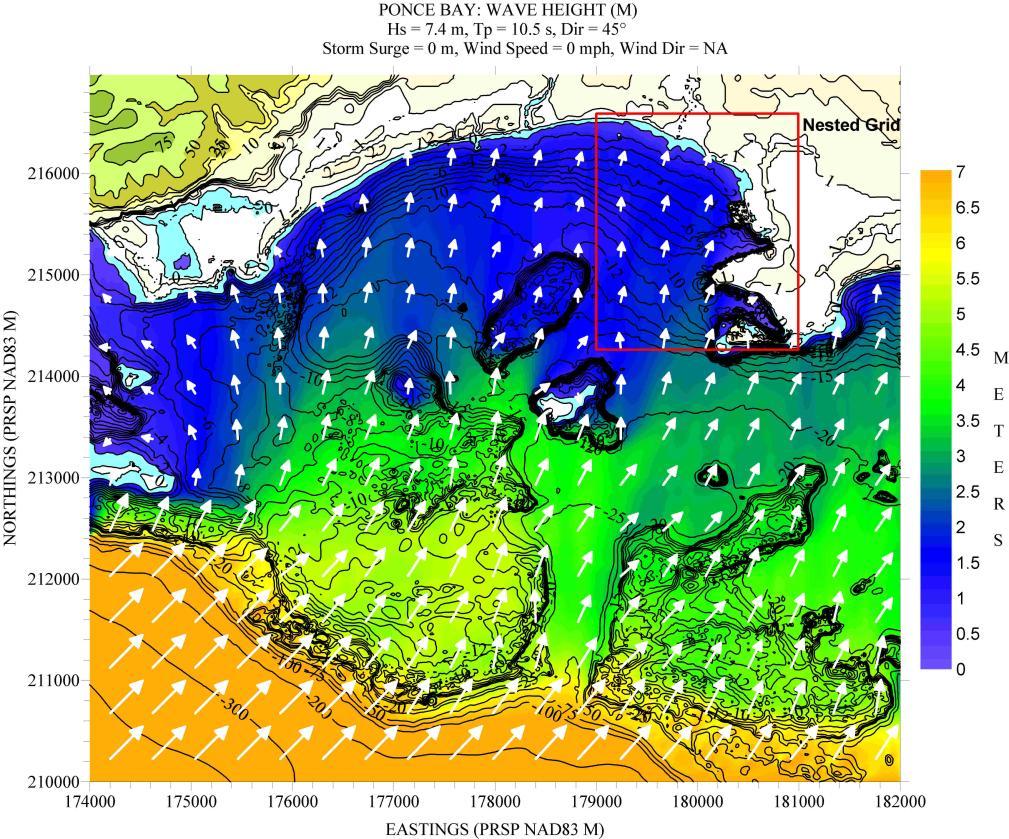
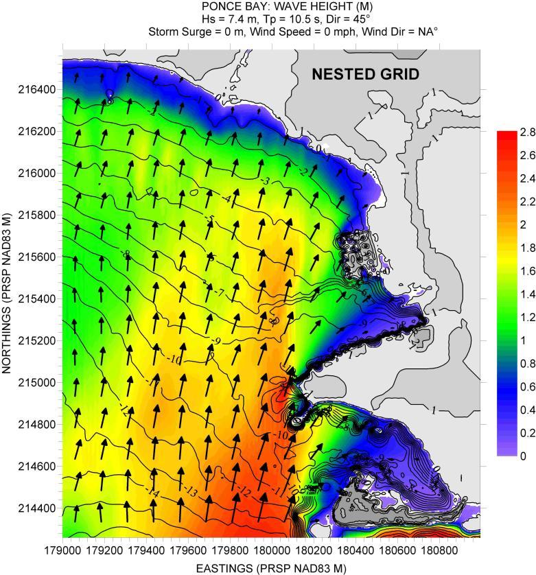
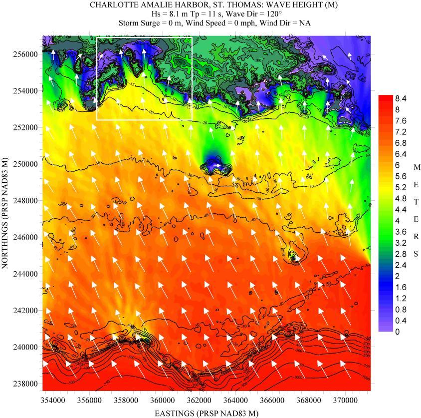
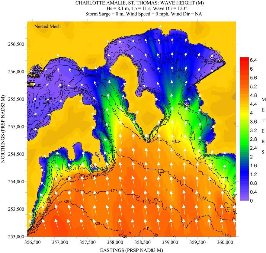
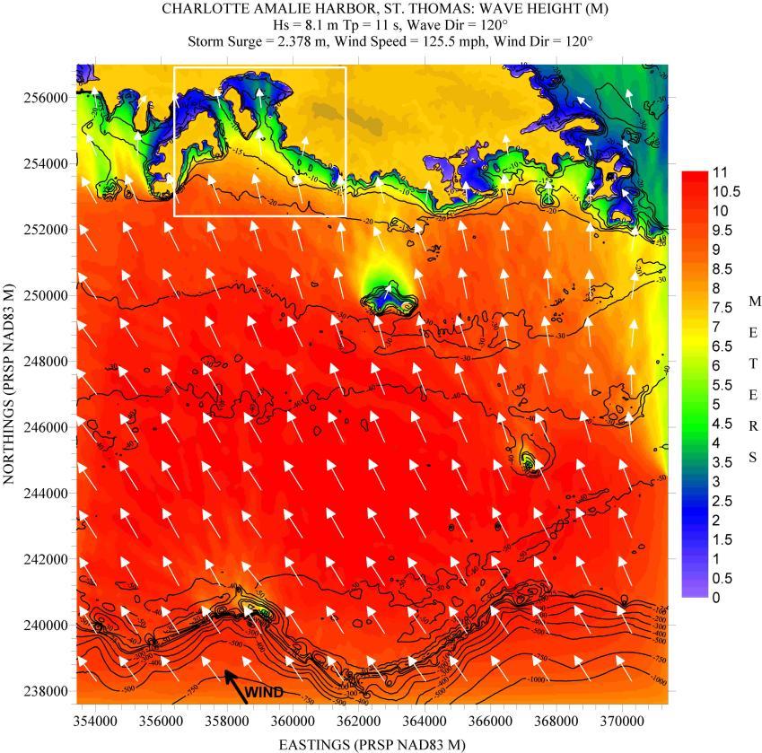
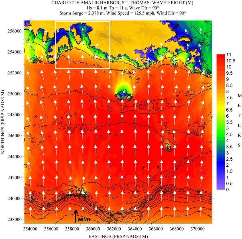
Figures 182 to 189 show contour plots of the Hs field for the simulations described along the top margin of each figure. Two deepwater wave directions were considered: waves from the southeast and from the south. The figures, together with Figure 190, show that large waves (4 - 5 m) are capable of reaching the entrance to both channels even under no storm surge and wind conditions. On East Gregerie Channel this can continue all the way up to Transect 2, with Hs between 2 - 2.5 m.
Along the channel leading to the main bay of Charlotte Amalie, wave energy seems to dissipate somewhat better (compare Transects 2 and 4), but not much (again, for no storm surge and wind conditions), with Hs values hovering around 2 m. Well inside the bay, Transect 5, waves hover around 1 - 1.5 m under no storm surge and no wind conditions, implying some good protection for these conditions.
Under storm surge and wind conditions things are very rough along East Gregerie Channel, with Hs values reaching 4 - 4.5 m along Transect 2 well inside the channel. Along the main channel to the main bay of Charlotte Amalie things are not much different, with Hs values between 2 - 3.5 m along Transect 4. Deep inside Charlotte Amalie Bay (Transect 5), under storm surge and wind conditions, we can see Hs values hovering between 2.5 to 3 m, decaying at both ends of the transect.
179. Posting showing location of bathymetry and topography values for Charlotte Amalie
180. Depth contour plot of outer computational grid for Charlotte Amalie Bay, St. Thomas. Also shown is the outline of the nested grid.
Figure
Bay, St. Thomas, USVI.
Figure
top margin of figure.
Figure 181. Depth contour for nested computational grid for Charlotte Amalie, St. Thomas.
Figure 182. Hs contour plot for Charlotte Amalie, St. Thomas, based on the scenario listed along the
Figure 183. Hs contour plot for (nested) Charlotte Amalie, St. Thomas, based on the scenario listed along the top margin of figure.
Figure 184. Hs contour plot for Charlotte Amalie, St. Thomas, based on the scenario listed along the top margin of figure.
Figure 185. Hs contour plot for (nested) Charlotte Amalie, St. Thomas, based on the scenario listed along the top margin of figure.
Figure 186. Hs contour plot for Charlotte Amalie, St. Thomas, based on the scenario listed along the top margin of figure.
Figure 187. Hs contour plot for (nested) Charlotte Amalie, St. Thomas, based on the scenario listed along the top margin of figure.
Figure 188. Hs contour plot for Charlotte Amalie, St. Thomas, based on the scenario listed along the top margin of figure.
Figure 189. Hs contour plot for (nested) Charlotte Amalie, St. Thomas, based on the scenario listed along the top margin of figure.
Figure 190. Significant wave height “slices” for Charlotte Amalie Bay, St. Thomas.
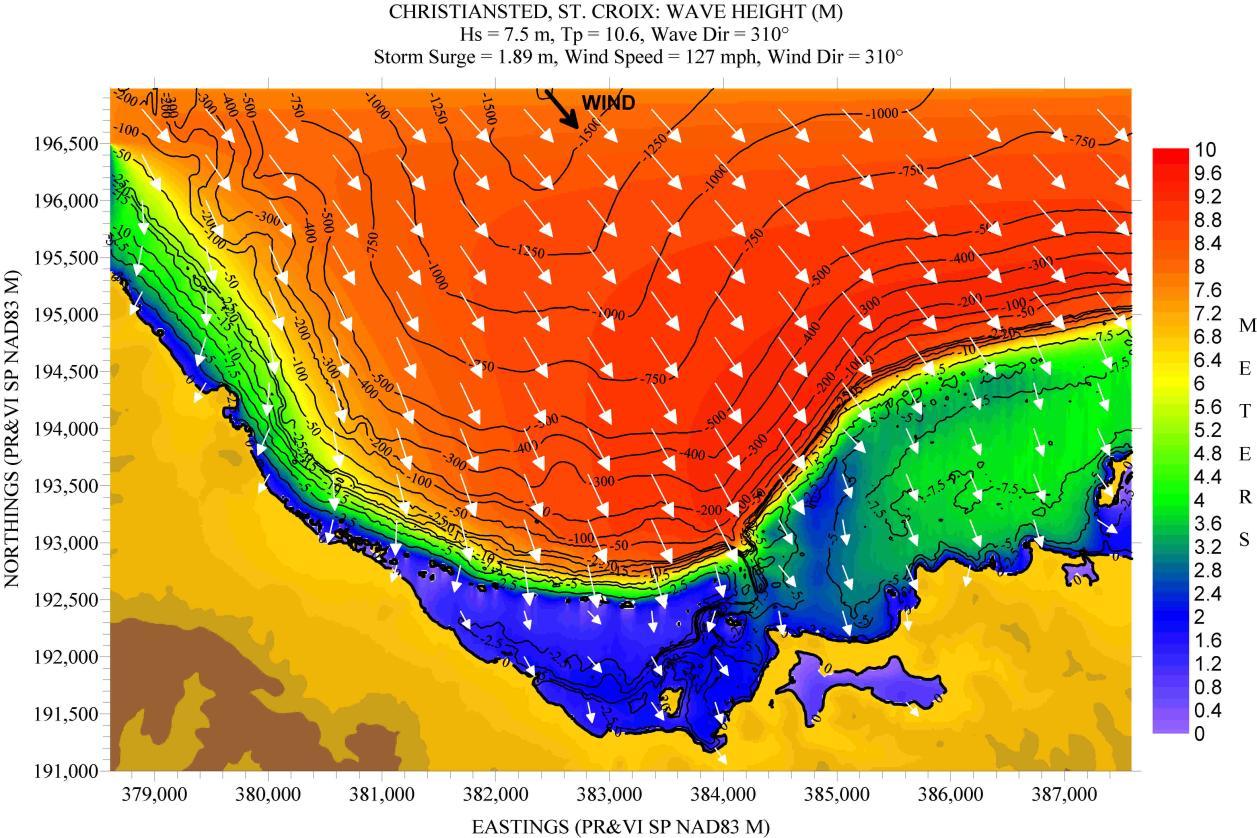
CHRISTIANSTED, ST. CROIX, USVI
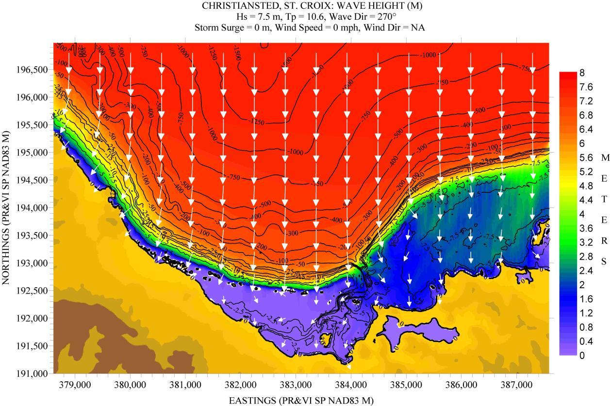
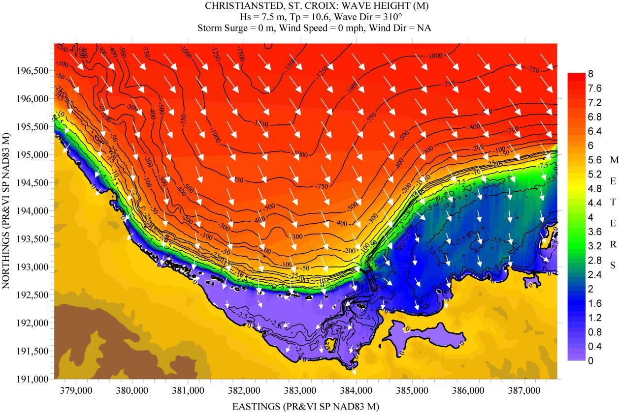
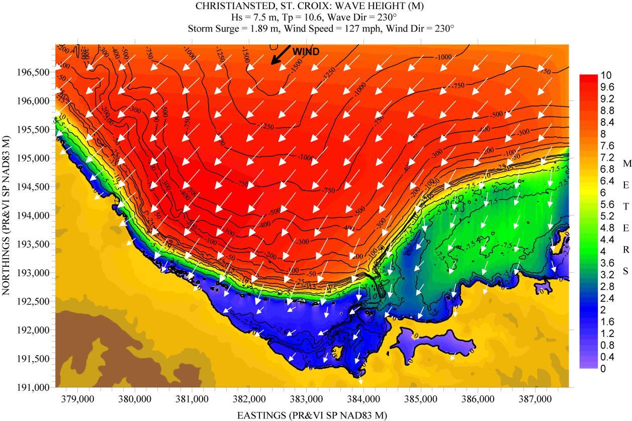
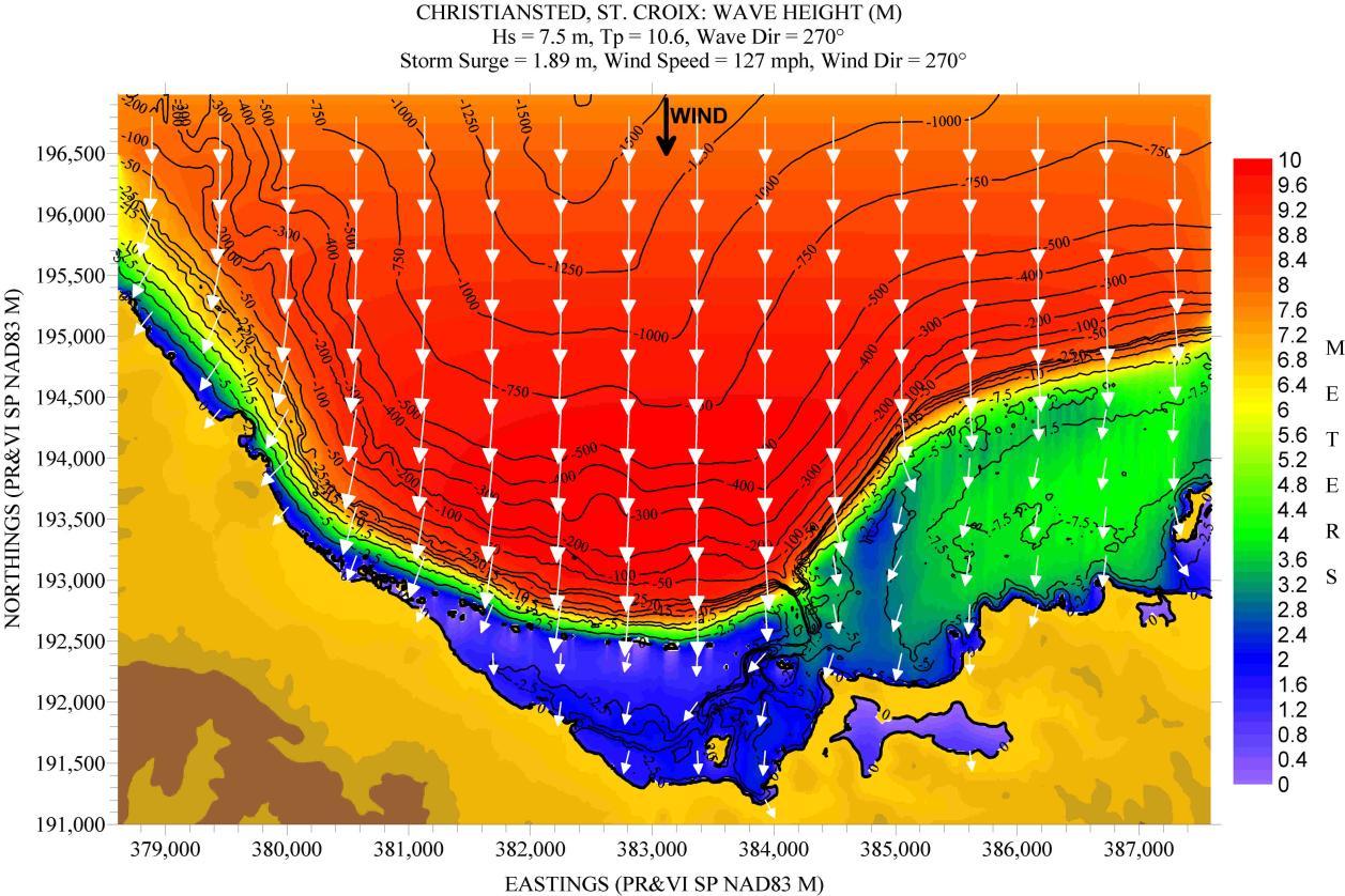
Figure 191 shows the locations where bathymetry and topography data are available. Figure 192 shows a depth contour plot of the computational grid, and the “slice” to obtain Hs values. It can be seen that this location is protected by a natural breakwater consisting of offshore reefs fronting the location practically all along its length. Deepwater waves propagating from the northeast, north, and northwest were simulated.
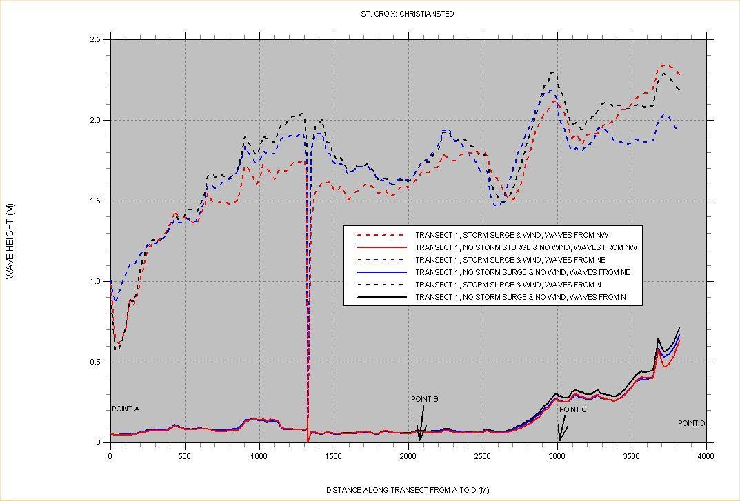
Figures 193 to 198 show contour plots of the Hs field for the conditions described along the top margin of each figure. The figures corroborate the statement above about the protection afforded by the natural breakwater, even though the shelf width is very narrow. Figure 199 shows the Hs variability along the “slice” shown in Figure 192. It shows that under no storm surge and no wind conditions, practically nothing penetrates through, irrespective of the offshore wave direction. Under storm surge and wind conditions Hs starts with half a meter at the western end of the slice (Point A), increasing to 1.5 - 2 m at halfway between Points A and B, and hovering around these two values until Point C, where it increases to around 2 m. Thus we can conclude that this location is well protected.
Figure 191. Posting showing location of bathymetry and topography values for Christiansted Bay, St. Croix.
Figure 192. Depth contour plot of computational grid for Christiansted Bay, St. Croix.
margin of
Figure 193. Hs contour plot for Chrsitiansted, St. Croix, based on the scenario listed along the top
figure.
Figure 194. Hs contour plot for Chrsitiansted, St. Croix, based on the scenario listed along the top margin of figure.
Figure 195. Hs contour plot for Chrsitiansted, St. Croix, based on the scenario listed along the top margin of figure.
Figure 196. Hs contour plot for Chrsitiansted, St. Croix, based on the scenario listed along the top margin of figure.
Figure 197. Hs contour plot for Chrsitiansted, St. Croix, based on the scenario listed along the top margin of figure.
Figure 198. Hs contour plot for Chrsitiansted, St. Croix, based on the scenario listed along the top margin of figure.
199. Significant wave height “slices” for Christiansted Bay, St. Croix.
Figure
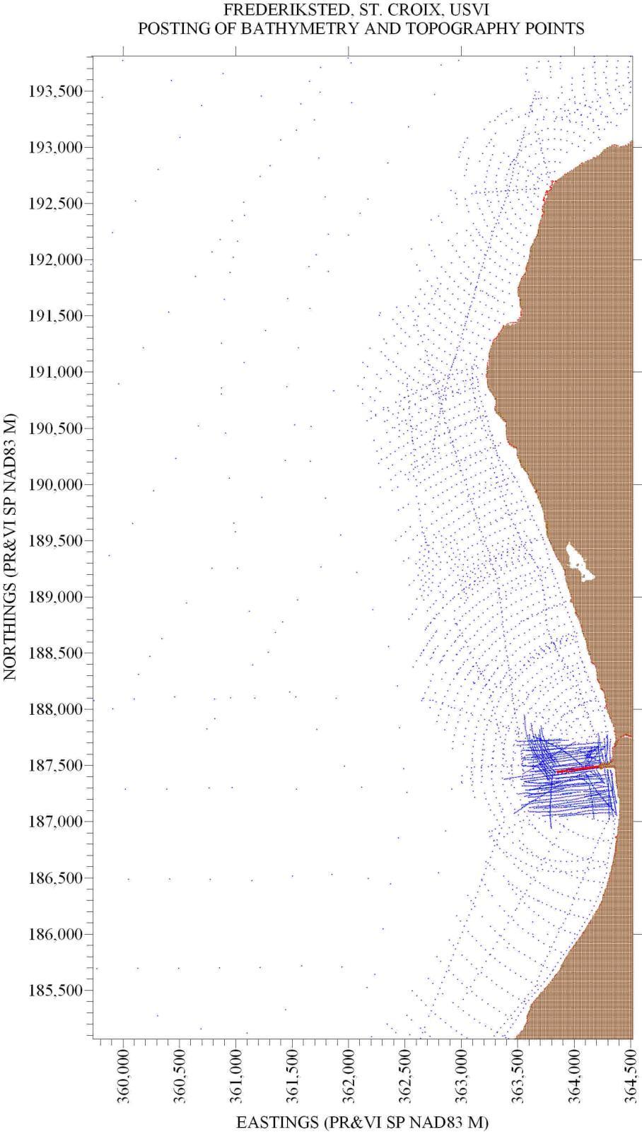
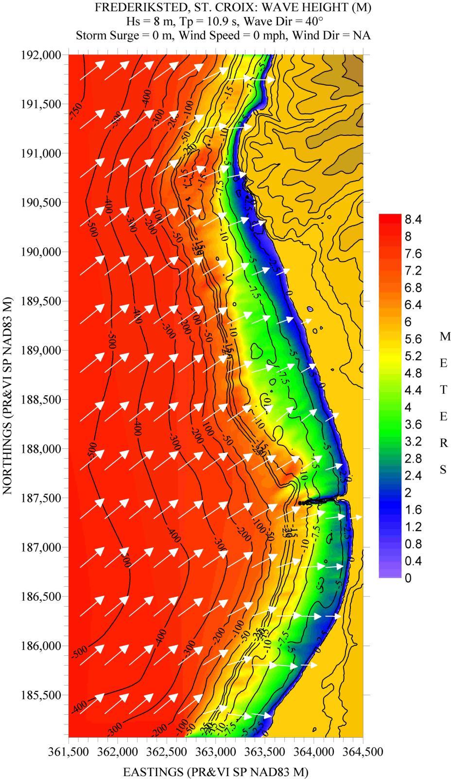
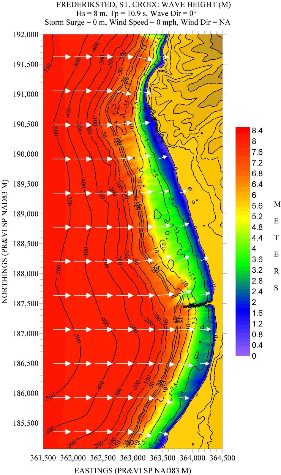
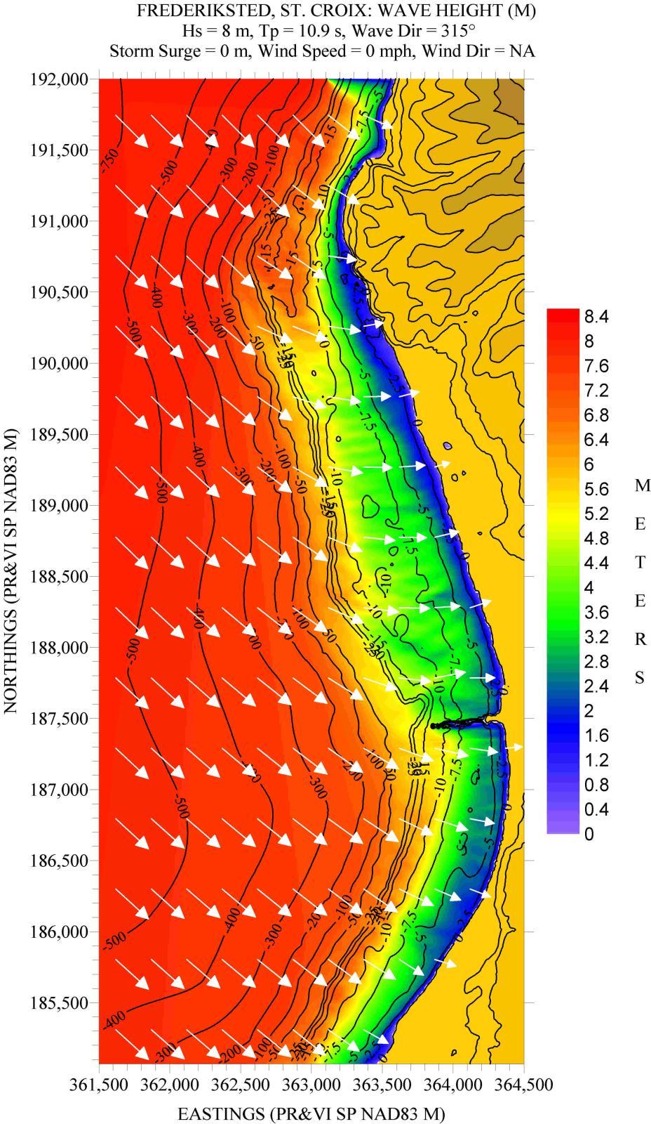
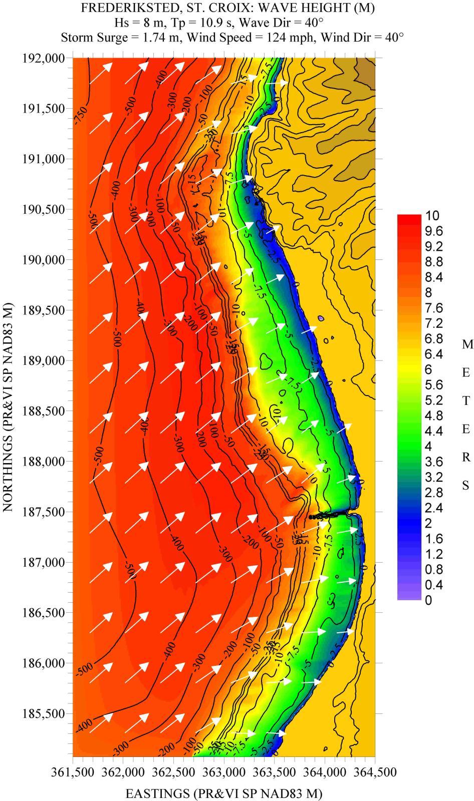
FREDERIKSTED, ST. CROIX, USVI
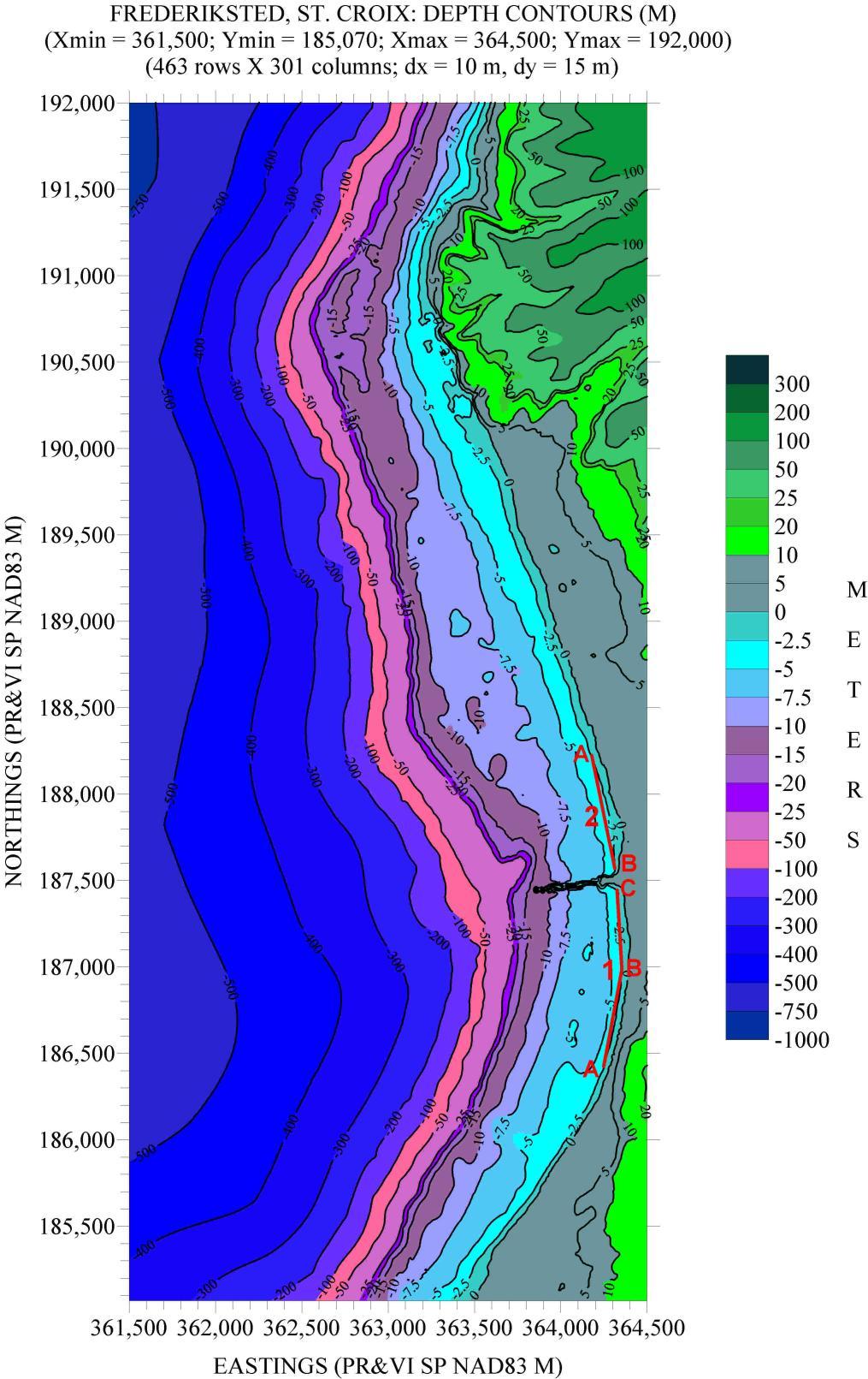
Figure 200 shows a posting of the locations where bathymetry and topography are available, and Figure 201 shows a depth contour plot of the computational grid (with the two “slices” for obtaining Hs values) Figures 202 to 207 show the results of the simulations for the scenarios described along the top margin. Three deepwater wave directions were simulated: from the northwest, west, and southwest.
This location is similar to Aguadilla, with a very narrow shelf and a very exposed coastline. Very large waves crash very close to the coastline. Two “slices” were used, centered along the pier at the location. Figure 208 shows that waves varying between 2 and 3.5 m break very close to the MSL shorelines, depending on whether a storm surge is present or not. It is obvious that this is a very exposed location.
200. Posting showing location of bathymetry and topography values for Frederiksted Bay, St. Croix.
Figure
Figure 201. Depth contour plot of computational grid for Frederiksted Bay, St. Croix.
202.
for
on the scenario listed along the top margin of figure.
Figure
Hs contour plot
Frederiksted, St. Croix, based
203.
for
based on the scenario listed along the top margin of figure.
Figure
Hs contour plot
Frederiksted, St. Croix,
204.
for
on the scenario listed along the top margin of figure.
Figure
Hs contour plot
Frederiksted, St. Croix, based
205.
plot for
based on the scenario listed along the top margin of figure.
Figure
Hs contour
Frederiksted, St. Croix,
for
on the scenario listed along the top margin of figure.
Figure 206. Hs contour plot
Frederiksted, St. Croix, based
the scenario listed along the top margin of figure.
Figure 207. Hs contour plot for Frederiksted, St. Croix, based on
Figure 208. Significant wave height “slices” for Frederiksted, St. Croix.
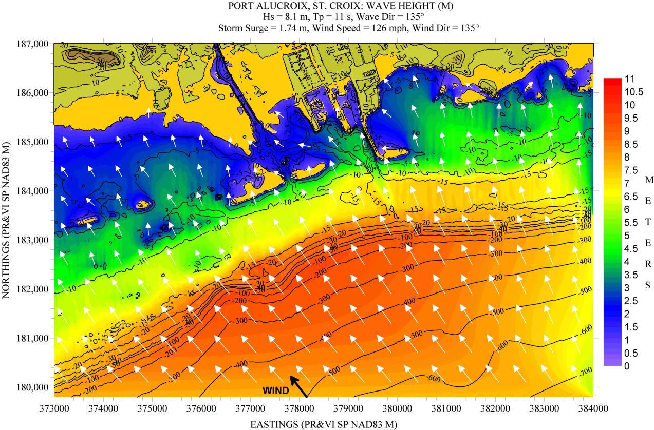
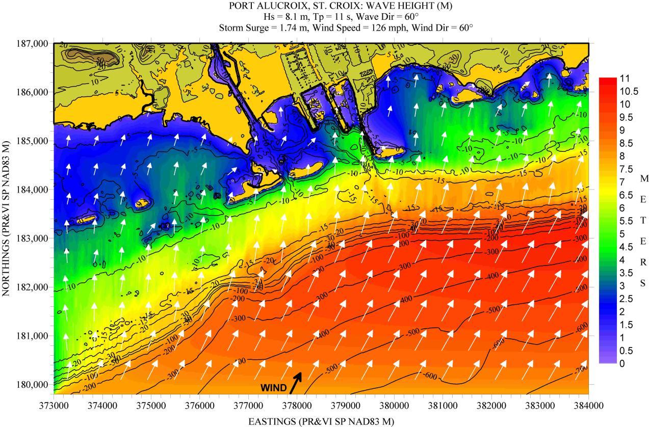
PORT ALUCROIX, ST. CROIX, USVI
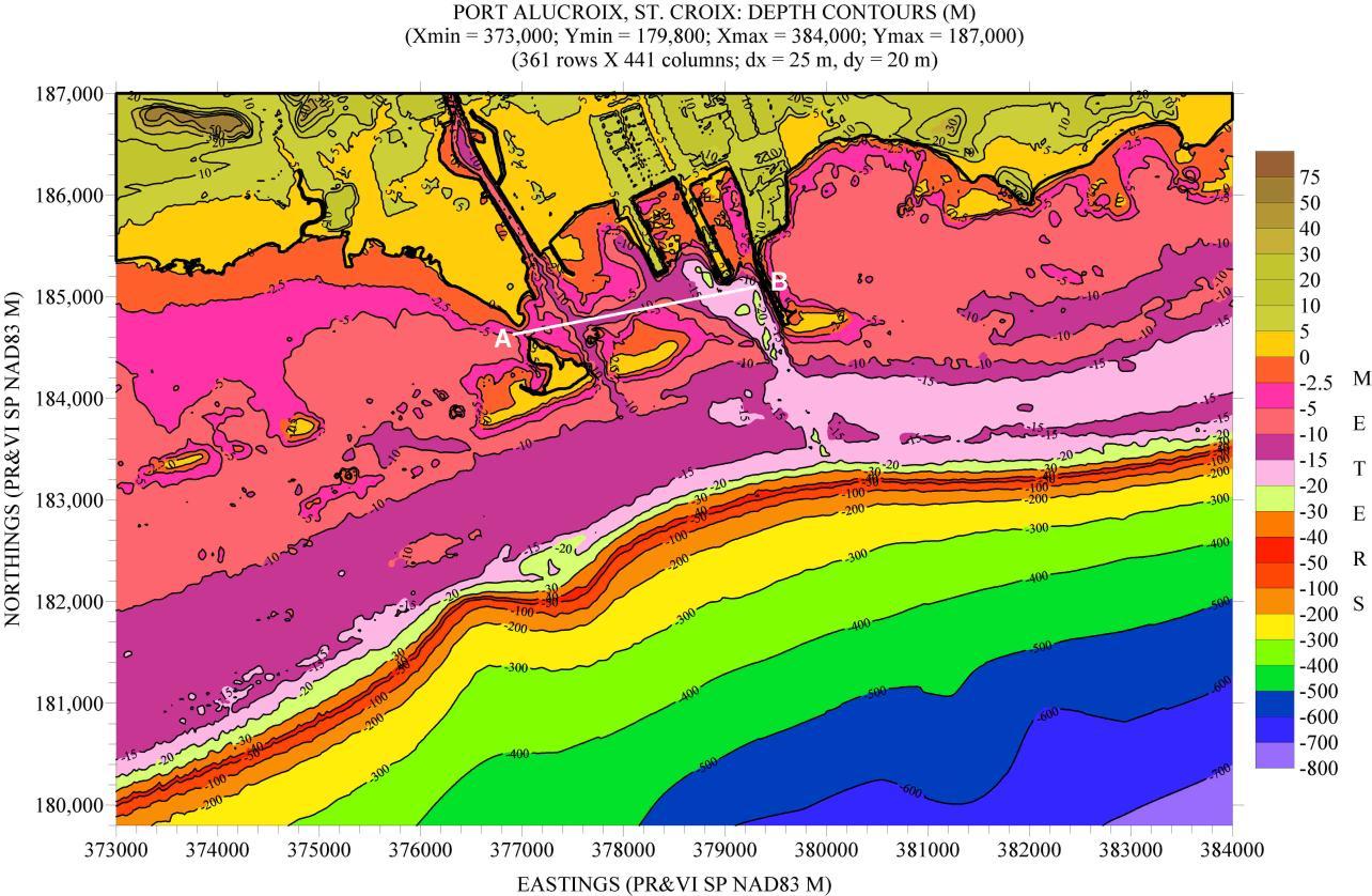
Figure 209 shows a posting of the bathymetry and topography locations for this site. Figure 210 shows a depth contour plot of the computational grid with the “slice” location . This is another location with a very narrow shelf and unprotected with the exception of a fringing reef (called Long Reef) protecting the entrance to the Krause Lagoon Channel.
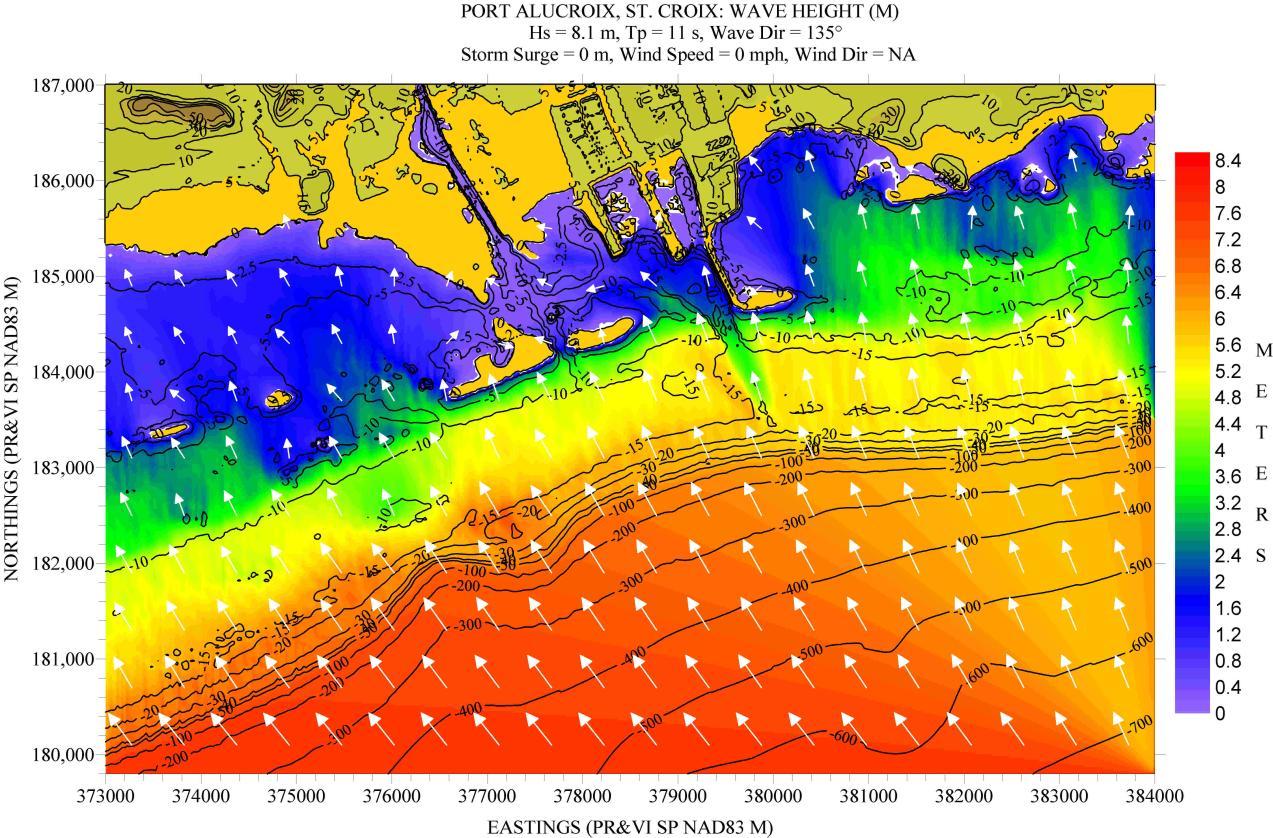
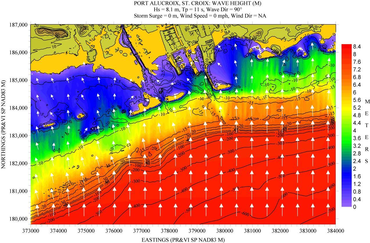
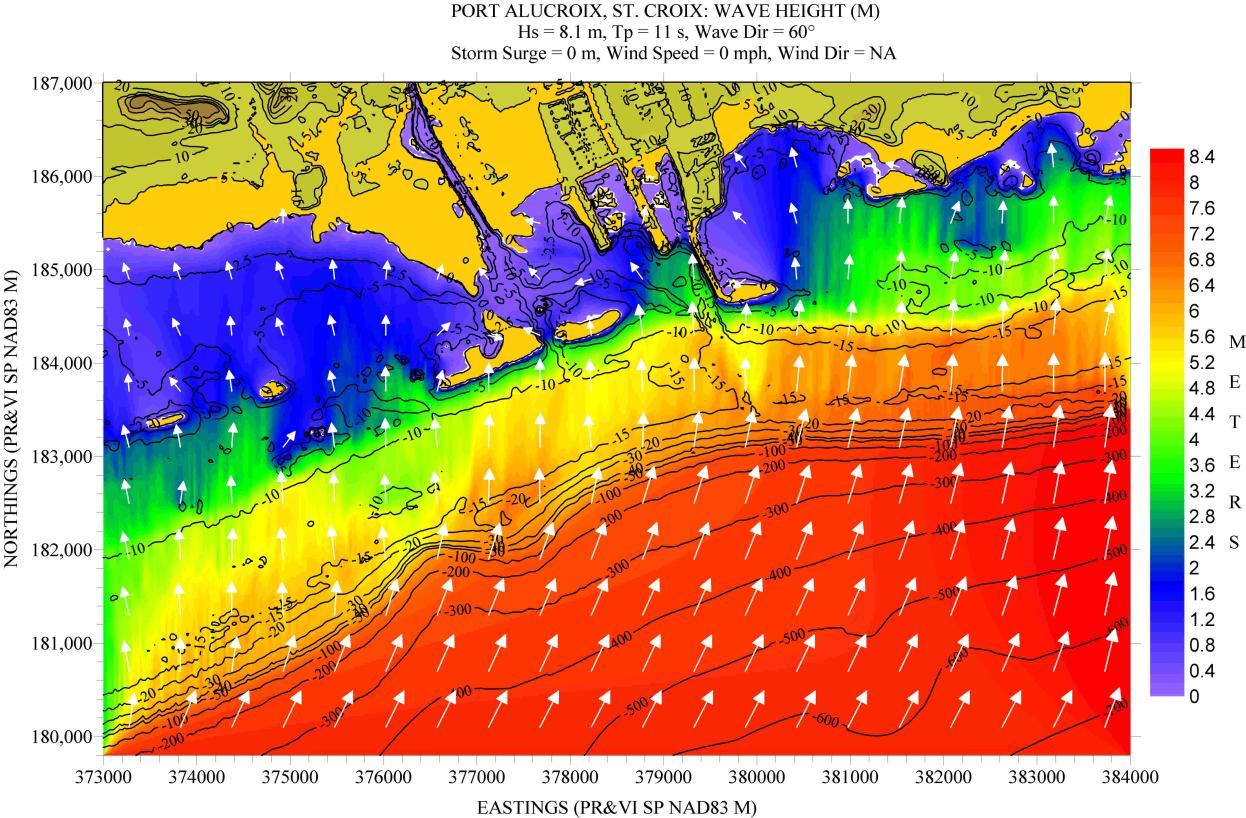
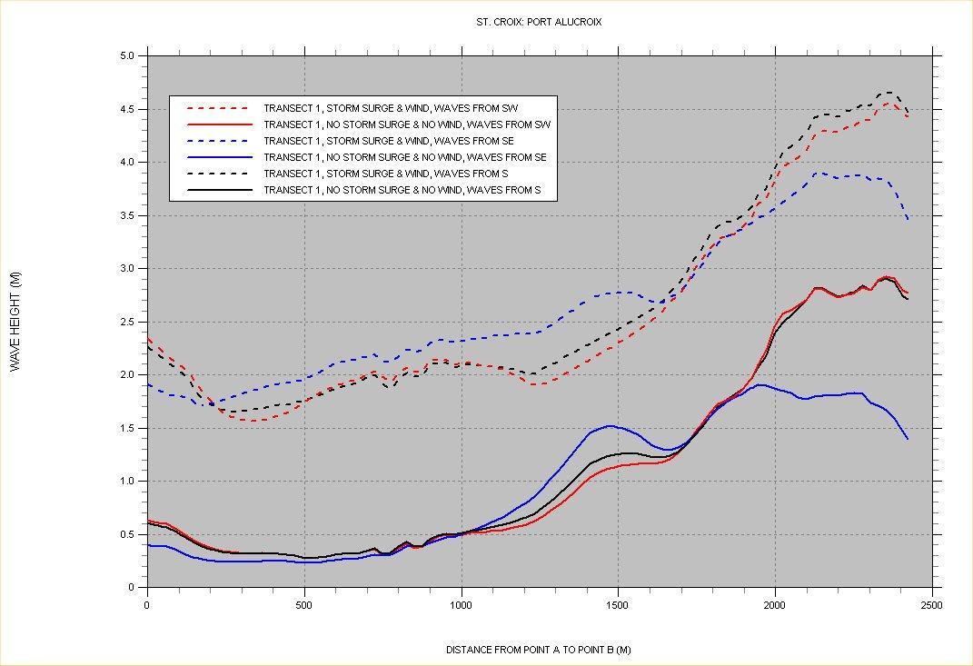
Three deep water wave directions were simulated: waves from the southeast, south, and southwest. Figures 211 to 216 show the results for the scenarios listed along the top of each figure. Figure 217 shows the Hs variation along the “slice”. As expected, under no storm surge conditions Long Reef offers good protection to the western side of the transect, but once outside its protection Hs values start to increase rapidly. For waves from the south and southeast Hs values on the eastern side (close to Point B) hover around 2.75 m.
When a storm surge is added, submerging the reef, then, in combination with the strong wind forcing, Hs values on the previously well protected back-side increased to around 2 m, while on the eastern side increase to around 4.5 m.
209. Posting showing location of bathymetry and topography values for Port
Figure
Alucroix, St. Croix.
Figure 210. Depth contour plot of computational grid for Port Alucroix, St. Croix.
Figure 211. Hs contour plot for Port Alucroix, St. Croix, based on the scenario listed along the top margin of figure.
Figure 212. Hs contour plot for Port Alucroix, St. Croix, based on the scenario listed along the top margin of figure.
Figure 213. Hs contour plot for Port Alucroix, St. Croix, based on the scenario listed along the top margin of figure.
Figure 214. Hs contour plot for Port Alucroix, St. Croix, based on the scenario listed along the top margin of figure.
Figure 215. Hs contour plot for Port Alucroix, St. Croix, based on the scenario listed along the top margin of figure.
Figure 216. Hs contour plot for Port Alucroix, St. Croix, based on the scenario listed along the top margin of figure.
Figure 217. Significant wave height “slices” for port Alucroix, St. Croix.
CONCLUSIONS
This study should be seen as a first, and preliminary, attempt to estimate the wave climatology inside the main bays, ports, and harbors in Puerto Rico and the USVI under extreme weather (i.e., hurricane) conditions. Being an island, we depend a lot on our port infrastructure, and events like Hurricane Hugo (especially its effect in San Juan and Culebra’s bays), was the motivation for this study.
We can conclude that there are bays which are obviously well exposed to big wind waves, in some cases not even requiring a wave simulation to reach this conclusion. Of the ones studied we can include in this category Arecibo, Aguadilla, and Frederiksted (St. Croix).
Then there are the ones on the opposite extreme in that their geometry and shape lead one to conclude beforehand that they are well protected. Of the ones studied, the following fall in this category: Guanica, Jobos, Las Mareas, and Puerto de Yabucoa.
Then are the ones that only a simulation will help in clarifying its exposure. And in this case, results vary as follows:
San Juan Bay – well protected by its narrow entrance channel, but waves generated inside the bay can do some damage, as seen during Hurricane Hugo.
Fajardo North (Bahía de Fajardo) – moderate protection Fajardo Center – waves as high as 3 m can reach the breakwater at Puerto del Rey Marina Fajardo South (Ensenada Honda, a.k.a. Roosevelt Roads, and Bahía de Puerca) – large waves (3 m or higher) expected when strong winds blow along its entrante channel axis)
Ponce Bay – large waves (3 m) can penetrate the deeper parts inside the bay under the extreme weather conditions assumed here.
Guayanilla Bay – the same as for Ponce Bay, large waves (3 m and higher) can penetrate into the deeper parts of the bay under extreme weather conditions.
Boquerón Bay – large waves (2.5 m or higher) can penetrate into the deeper parts of the bay under extreme weather conditions.
Puerto Real Bay – well protected even under extreme weather conditions.
Mayaguez Bay – the northern half of the bay is much more exposed than the southern half. In the deeper parts of the northern half of the bay waves higher than 3.5 m can be seen in the simulations.
Ensenada Honda, Culebra – this bay is well protected by its narrow entrance channel and the myriad of offshore reefs protecting this entrance.
Christianted, St. Croix – this bay is well protected by the fringing reefs lying offshore.
Port Alucroix, St. Croix – the western side of the port is relatively well protected by an offshore fringing reef (Long Reef), but on its eastern side, not being protected by the reef, large waves (2.5 m under no storm surge and no wind conditions; 4.5 m under both conditions) can be seen in the results.
It is hoped that the results shown here will serve as a first, and rough, guide to anyone interested in knowing the extreme wave climatology that can be expected inside these bays and ports.
ACKNOWLEDGMENTS
This project was supported by the Sea Grant Program of the University of Puerto Rico. Special thanks should be given to Dr. Juan Carlos Ortiz, a former Ph.D. student at the Department of Marine Sciences, who expedited my learning of the intricacies of the SWAN model. I would also like to thanks the Faculty of Arts and Sciences, and its Department of Marine Sciences, for the release time given to me for working on this project.
REFERENCES
Mercado, A., 1994. On the use of NOAA’s storm surge model, SLOSH, in managing coastal hazards – the experience in Puerto Rico. Natural Hazards, 10:235-246.