Science Research Journal, Vol 1, 2021

SCIENCE RESEARCH JOURNAL Volume 1

2021 SCIENCE RESEARCH JOURNAL Volume 1

‘Challenging the Status

Quo in Science’

was our Science goal for 2021. In all our Science lessons we encourage students to be active learners; by asking questions, as questions are often more important than the answer. How best do we prepare our students for an uncertain future? How do we teach the skills needed to solve problems that we don’t even know are problems yet? What does it really mean to equip our students with 21st century skills?

The events of 2021 have more than ever shown us the importance of Science, everyone needs Science. We need our students to be scientifically literate, to think critically, to be creative, to ask questions, to solve problems, to be curious and to know that Science transforms lives. This year like no other we have been able to witness the importance and value of scientific research. Scientific research uses the scientific method to prove a hypothesis, claim or observation, it develops and promotes knowledge and information, it drives innovation and allows us all to live better and longer lives.

A number of our IB, HSC and Yearr 10 Science students this year have conducted some exceptional scientific research. They developed their own question, conducted some background information, carefully planned and conducted their valid and reliable methodology to test their research, collected their data and analysed it before drawing their conclusions. I am pleased and proud to say that our students have amazed me with the quality of their scientific reports, they have conducted some real world genuine scientific research and in the process have learnt a lot about their world and themselves as learners and become more scientifically literate in the process.

I would like to congratulate each student for their efforts and contributions and I am happy that they have learnt what it means to be a research scientist and enjoyed the challenges that this journey allowed them to experience.

I hope the Santa community enjoys reading the students’ scientific research papers as much as I did.

MOIRA DE DOMENEGHI Head of Science

Contents

Investigation of the Relationship Between the pH of a Methanoic Acid Buffer Solution and the Rate Constant on the Inversion of Sucrose

Anastasia Gikas, Year 12 IB Chemistry HL 1

Investigation of the Effect of Impedance on the Power Factor of an RLC Circuit Anastasia Gikas, Year 12 IB Physics HL 16

Comparing the viscosity of four different liquids Rosanna Cartwright, Year 10 Science 31

The effect of sugar concentration on fermentation Sophie Rigon, Year 10 Science 55

Investigating the relationship between different colour noises and the amount of deep sleep they stimulate Maree Sialepis, Year 10 Science 65

An invesitgation into oxygen exposure and ethanoic acid formation in red wine Hannah Svoboda, Year 12 IB Chemistry SL 73

Measuring Coral Replantation Efficacy Eliose Struthers, Year 12 HSC Science Extension 86

Investigating how the Height from which Water falls impacts the amount of Hydropower produced Isabella Azzopardi, Year 12 IB Physics SL 100

Detremination of Vitamin C Mass by Titration in Different Fruits Maya Lee, Year 12 IB Biology HL 114

Investigating the Effect of Leaf Foliage Density on Radiant Heat Rachel Frecker, Year 12 IB Biology SL 127

Mona Talks Corona: The Automated Chatbot for Adolescents

Joanna Benedict, Sonya Jayatatillake, Victoria Kim, Lordeana Leonard, Sophia Witting, Winners of the Biotech Future 2021 competition 139

Investigation of the Relationship Between the ���� of a Methanoic Acid Buffer Solution and the Rate Constant of the Inversion of Sucrose

Exploration

Research Question

What is the relationship between the pH (2.00, 4.00, 6.00 / ± 0.01) of a methanoic acid buffer solution and the rate constant �� (mol 1 dm3 s 1) of the inversion of sucrose, calculated from the angle of rotation ��(��) using the formula ��(��) =��0����([C12H22O11]0 [H+]0)�� ?

Introduction and Rationale

Sucrose (C12H22O11), also known as saccharose, decomposes into a mixture of glucose and fructose called “invert sugar” when dissolved in an acidic solution. This reaction is known as the inversion of sucrose because it causes a rotation of the plane of polarisation; the sucrose solution is dextrorotatory (D, rotation towards the right), while the mixture of glucose and fructose is levorotatory (L, rotation towards the left) (Physical Chemistry Laboratory, 2018). As this reaction occurs, the taste of sucrose becomes increasingly sweeter and less likely to be spoiled by numerous microorganisms than other types of sweeteners (Sale & Skinner, 1922). In addition, it prevents the crystallisation and moisture loss from the culinary products which contain it. Monitoring the rate and extent of sucrose inversion is important in order to retain flavour and texture in processed foods such as soft drinks, sweets and other products involving sweeteners. Since the presence of a Brønsted Lowry acid (H+) increases the rate of inversion, consideration of the acidity of a solution of sucrose is imperative in manufacturing, cooking, baking and food sciences.

When baking with my grandparents, I was exposed to various traditional desserts which involved different ways of sweetening. I found that using a different sugar or sweetener made a large difference to the overall taste, and became curious as to why, probing my inquiry into reactions with different sugars. Additionally, I was immediately intrigued when I started reading into organic chemistry, particularly stereoisomerism. Following further research into the applications of polarimetry, I discovered that my interest in saccharide chemistry could be paired with polarimetry to design an investigation which enables me to delve into both interests. As aforementioned, this also has many industrial and individual applications which interested me, and finding an ideal acidic pH for a quick rate of reaction which is commercially favourable will allow for efficient, large scale production.

Background

Methanoic or formic acid, HCOOH, is a weak acid with dissociation constant ���� =1.77×10 4 at 25.0ºC (Harned & Embree, 1934). In an aqueous solution, methanoic acid dissociates according to the equation: HCOOH (aq) + H2O (l) ⇌ H3O+ (aq) + HCOO (aq) with ���� being defined as the ratio of the equilibrium concentration of aqueous products to aqueous reactants: ���� = [H3O+][HCOO ]

[HCOOH]

A solution where a weak acid and its conjugate base (or a weak base and its conjugate acid) exist in non zero concentrations is called a buffer solution. Buffer solutions are represented by reversible reactions, where the concentration of either the acid, base, conjugate acid or conjugate base of a weak acid may change. The distinctive characteristics of buffer solutions is that they resist pH change if small amount of an acid or a base is added. Hence, they are important in regulating natural systems such as the pH of blood, the osmotic balance of cells and the biochemical composition of various foods (Brown & Ford, 2014)

The buffer system resulting from the dissociation of HCOOH involves the acid base pair HCOOH/HCOO . Hence, according to Le Chatelier’s principle, if the concentration of the conjugate base (HCOO ) is increased, the position of the equilibrium will favour the reactants. The concentration of the conjugate base may be increased by dissolving a methanoate salt, such as sodium methanoate (HCOONa).

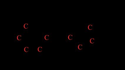
Following the addition of HCOONa, a new equilibrium is established, and the pH of the solution is expected to be higher as there will be a lower concentration of H3O+ (typically, the hydronium ion is written as H+). This phenomenon is known as the common ion effect (Clark et al., 2019) The [H+] affects the rate constant �� (and rate of reaction) in any reaction in which it is a reactant, such as the inversion of sucrose. The chemical reaction for sucrose inversion, or hydrolysis, can be seen in Figure 1.

C12H22O11 (aq) + H2O (l) + H+ (aq) → C6H12O6 (aq) + C6H12O6 (aq)

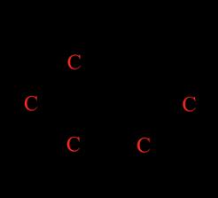
Figure 1: Reaction for the inversion of sucrose. Sucrose, glucose and fructose are all optically active organic compounds, meaning that when plane polarised light, or light in which the electric field vector oscillates only in one direction, passes through a solution of them, they cause it to rotate by a particular angle (Anton Paar GmbH, 2021). Optical activity arises due to the presence of chiral centres or carbon atoms bonded to four different atoms or groups, making them asymmetrical; the chirality of these saccharides is shown in Figure 2 below.

sucrose glucose fructose

Figure 2: Chiral centres of sucrose, glucose and fructose shown in red in their structural formulas. The device used to quantify optical activity is a polarimeter, which consists of a light source, a solution tube and two polarising filters along with a light detector. The monochromatic wave emitted is plane polarised, travelling in one orientation, and is then passed through the solution in the polarimeter’s tube (Brown & Ford, 2014). The plane is rotated by the chiral mixture and an analyser is used to determine rotation, then electrically processed by the photocell and displayed on the screen.

The polarimeter measures the angle of rotation �� of the mixture in the tube, also known as the observed rotation. This is done by displaying the change in angle of the plane of polarised light as it passes through the sample in the solution tube. The angle of rotation �� depends on the following factors: length of the polarimeter ��,concentrationof the solution in thetube �� andthespecificrotation [��]�� ��.Specificrotation([��]�� ��)isa constant physical property of an optically active compound that shows the magnitude and direction of the light’s plane rotation at a particular temperature �� and for a specific wavelength ��. If ��, �� and �� are kept constant, the angle of rotation will be directly proportional to the concentration of the sample in the tube, as shown below: �� =����[��]�� �� �� ∝ ��

In the inversion of sucrose, the rate law can be written as the product of the reactants’ concentrations raised to the power of their reaction order, with ��′ as the rate constant: rate=��′[C12H22O11]��[H2O]��[H+]��

Assuming that the concentration of water is excessively large in relation to the other reactants, it does not significantly change over the course of the reaction. It is therefore considered a constant. Furthermore, assuming that sucrose and H+ are first order reactants (making the overall reaction second order), and this is the only, rate determining step, the differential form of the rate law may be simplified to: rate=��[C12H22O11][H+] where �� is the rate constant with the given assumptions.

However,ina reaction where the concentrationsofthetwofirst orderreactants areunequal (suchas thesecond order reaction for sucrose inversion in this experiment), the integrated rate law must be utilised instead The integrated rate law is an expression derived from calculus and considers the changes in reactant concentration over time. It can be expressed as (Boundless Learning, n.d.):

ln([C12H22O11][H+]0 [H+][C12H22O11]0)=��([C12H22O11]0 [H+]0)��

where �� is the time after the reaction begins (in seconds), [C12H22O11]0 is the initial concentration of sucrose, and [H+]0 is the initial concentration of hydrogen ions. In this experiment, because the concentration of H+ is altered by changing the pH of the methanoic acid solution, the reactant concentrations are unequal and hence it is not possible to calculate the rate constant from the differential form of the rate law; thus, the integrated rate law will be used. In this second order reaction, it is impossible to isolate the concentration of a single reactant, as they both change in parallel. Rather, the ratio of the concentrations is considered. Let [C12H22O11] [H+] =��(��) ln��(��)+ln [H+]0 [C12H22O11]0 =��([C12H22O11]0 [H+]0)�� ln��(��)=��([C12H22O11]0 [H+]0)�� ln [H+]0 [C12H22O11]0 ��(��)=����([C12H22O11]0 [H+]0)�� ln [H+]0 [C12H22O11]0 ��(��) = ����([C12H22O11]0 [H+]0)�� �� ln [H+]0 [C12H22O11]0

= ����([C12H22O11]0 [H+]0)�� [H+]0 [C12H22O11]0

= [C12H22O11]0 [H+]0 ����([C12H22O11]0 [H+]0)��

As aforementioned, the angle of rotation �� is directly proportional to the concentration �� of a substance in a solution (Bora et al., 2018). It follows that if the concentration of the optically active sample changes over time, the angle of rotation will also be time varying. Therefore, the angle of rotation and concentration of the sample in the tube will be treated as functions of time, ��(��) and ��(��) respectively. The concentrations of multiple optically active reactants and/or products are changing in the sample in the polarimeter tube, so the measured angle of rotation is the sum of the mole fraction of each species. For the inversion of sucrose, the measured angle of rotation over time can be calculated using: ��(��)= ����������������(��) ������������(��) ���������������� + ����������������(��) ������������(��) ���������������� + ������������������(��) ������������(��) ������������������

As sucrose is being hydrolysed into glucose and fructose, the angle of rotation should gradually change. Initially, the (overall) angle of rotation should be equal to the angle of rotation of sucrose, as there are no products in the mixture. As the inversion progresses, more glucose and fructose are produced in a molar ratio of1:1.Considering theinitialangleofrotation ��0,andmeasuringhow ��(��)changesover timeasmoresucrose is being hydrolysed, it is possible to determine the change in concentration ratio of the reactants ��(��), where �� acts as the proportionality constant. ��(��)∝ ��(��) Let��0 =�� [C12H22O11]0 [H+]0 ��(��)= ��������([������������������]�� [��+]��)��

The above (bolded) function will thus be used to determine the value of the rate constant ��. The values of ��0 and ��(��) will be measured using a polarimeter, whilst the [C12H22O11]0 value is constant in all trials The [H+]0 is reliant on the pH of the buffer solution, and will have a different value which will be substituted into the equation at pH 2.00, 4.00 and 6.00.

Hypothesis

Increasing the pH of a 0.570 mol dm 3 methanoic acid buffer solution by adding HCOONa will increase the magnitude of the rate constant ��, yielding a less negative value. This is expected due to the common ion effect, where increasing the concentration of a product leads to an equilibrium position favouring the reactants This results in a lower [H+] and a higher pH. As the rate constant of the inversion of sucrose is increased in an acidic environment, higher pH should lead to a lower rate constant. The angle of rotation will be used to determine the rate of the inversion reaction as both sucrose and the products are optically active compounds.

Methodology

Variables

Table 1 details the independent variable in this experiment.

Table 1: Independent variable. Independent variable

pH of the methanoic acid solution

Variation method

The pH is changed by altering the concentration of HCOO in the reaction mixture, which affects the initial concentration of H+ according to Le Chatelier’s principle. The [H+]0 is determined from [H+]0 =10 pH, as seen in Appendix A.

Intervals (± 0.01) [��+]��

2.00 0.0100 4.00 100×10 4 6.00 1.00×10 6

The selection of methanoic acid is justified for multiple reasons. Firstly, it is a weak acid; strong acids have a constant pH independent of the conjugate base concentration, given they completely dissociate. Additionally, HCOOH is a liquid at room temperature (25.0ºC) and it inexpensive, readily available and relatively safe compared to more corrosive acids.

The dependent variable is elaborated on in Table 2.

Table 2: Dependent variable Dependent variable Measurement method

Rate constant of the inversion of sucrose

Calculated from curve fitting; the equation ��(��)=��0����([C12H22O11]0 [H+]0)�� will be used with ��, ��0 and ��(��) being the experimental measurements. This process will be repeated for the three pH levels.

Table 3 explains the controlled variables

Table 3: Controlled variables. Controlled variable Control method

Justification Units

By observing how the angle of rotation of the mixture changes over time, the rate of change of sucrose concentration can be determined. The pH affects the magnitude of the rate constant in the inversion.

mol 1 dm3 s 1 as calculated in the data processing

Stirring process. Be consistent in the vigorousness and duration of stirring the solutions for all trials

Same polarimeter, electronic balance and pH probe used.

Temperature of the solution and surroundings.

Use the Atago Polax D polarimeter, A&D Mercury FX 400 electronic balance and EZDO 7200 pH probe

All trials will be carried out in the same, air conditioned laboratory at approximately 25.0ºC. All solutions used should be kept at the same location. The polarimeter ensures a thermostable environment in the tube during the reaction.

Justification

This ensures that the concentrations are uniform throughout the solution

Errors in calibration or faulty readings may exacerbate systematic errors.

The temperature �� affects the specific rotation, which in turn affects the angle of rotation, as seen in: �� =����[��]�� ��

Polarimeter tube length.

Use the same polarimeter tube of length 100 mm in all trials.

Wavelength of light. Set the polarimeter’s light source to emit monochromatic light of 589 nm.

Type of acid used. HCOOH is used in all trials.

Initial concentration of C12H22O11 and HCOOH.

Risk Assessment

Prepare the solutions so that equal concentrations are used in each trial, as detailed in the method.

The length of the tube �� affects the angle of rotation as per: �� = ����[��]�� �� .

The wavelength �� affects the specific rotation, which in turn affects the angle of rotation, as seen in: �� =����[��]�� �� .

Different acids have different ���� values, which would affect the rate of reaction.

The initial concentrations affect the angle of rotation of the mixture, as per: ��(��)=��0����([C12H22O11]0 [H+]0)��

This ensures that only the concentration of H+, and hence the independent variable pH, is affecting the rate constant.

Table 4 details hazards, risks posed and mitigations to establish a safe experimental environment.

Table 4: Risk assessment.

Hazard Risk Posed Mitigation

Use of a glass beaker, measuring cylinders and a stirring rod.

Given that glass is very fragile, if dropped on any hard surface, it may shatter and cause punctures, cuts, and infections at the wound.

Confirm, prior to beginning the experiment, that none of the glassware is severely scratched or cracked. Wear a laboratory coat, safety glasses, latex gloves and enclosed shoes for added protection. Handle all glassware with care. Have a first aid kit nearby. If the beakers or stirring rods happen to break, use a dustpan to remove shattered pieces.

HCOOH is corrosive.

Dropping the polarimeter on the ground or on someone’s foot.

An acid spill may cause skin burns, eye irritation and/or damage to surroundings.

The polarimeter is heavy and may result in injuries if it falls on someone. It can also fall on the ground where someone may trip over it, or may cause structural damage.

Wear a laboratory coat, safety glasses, gloves and enclosed shoes for added protection. Handle acid with care. Ensure that a spill neutralisation reagent is available at the laboratory. Solutions may be disposed of ethically by simply pouring down the sink (NSW Education Standards Authority, n.d.).

Place the polarimeter away from the edge of the laboratory bench and ensure that only the experimenter is near the device. Neatly collect any loose hanging wires to mitigate trip hazard.

Reagents

The reagents used in this experiment are shown in Table 6.

Table 6: Reagent list.

Quantity

Reagent

5.130 g Pure sucrose 100 cm3 Methanoic acid 90% w/w, 23.6 mol dm 3 stock (The Nest Group, Inc., 2016)

9.905 g Sodium methanoate powder ≥ 99% 4.04 dm3 Distilled water

Method

The pH calculations are shown in Appendix A, and all other relevant calculations used for the stoichiometric relationships in the method can be seen in Appendix B.

1. Calibrate the polarimeter according to the instructions.

2. Prepare a 4.14 dm3 solution of 0.570 mol dm 3 HCOOH by adding 4.04 dm3 of distilled water to the stock 23.6 mol dm 3 solution in the 5 dm3 beaker. To attain a precise volume, transfer 4.00 dm3 of distilled water via the large 5 dm3 beaker, and add 0.04 dm3 of distilled water using a 50 cm3 measuring cylinder.

Part A: pH= 2.00

3. Using a pipette, transfer 10 cm3 of the diluted HCOOH solution into a 25 cm3 measuring cylinder.

4. Add 0.342 g of C12H22O11 into the 25 cm3 measuring cylinder. Stir thoroughly using a stirring rod until fully dissolved.

5. Use 1 strip of the universal indicator paper to ensure that the pH has reached 2.00 (light red). Confirm the pH value using the pH probe.

6. Turn on the sodium lamp of the polarimeter and transfer the mixture into the polarimeter’s observation tube.

7. Record the angle of rotation as soon as the tube is inserted by adjusting the eyepiece lens until the field of view attains a uniform colour (yellow), and then every minute for 20 minutes.

8. Repeat steps 3 7 for four more trials.

Part B: pH= 4.00

9. Using a pipette, transfer 10 cm3 of the diluted HCOOH solution into another 25 cm3 measuring cylinder.

10. Add 0.476 g of HCOONa into the 25 cm3 measuring cylinder from step 9 Stir thoroughly until fully dissolved.

11. Repeat steps 5 7, instead ensuring that the pH has reached 4.00 (light orange).

12. Repeat steps 9 11 for four more trials.

Part C: pH= 6.00

13. Using a pipette, transfer 10 cm3 of the diluted HCOOH solution into another 25 cm3 measuring cylinder.

14. Add 1.505 g of HCOONa into the 25 cm3 measuring cylinder from step 13 Stir thoroughly until fully dissolved.

15. Repeat steps 5 7, instead ensuring that the pH has reached 6.00 (light green).

16. Repeat steps 9 11 for four more trials

Results and Analysis

Raw Data

Qualitative Data

For all trials at all pH levels, a strip of universal indicator paper was used to qualitatively confirm that the buffer solution had the predicted pH. It was observed that for the pH= 2.00 solutions, the indicator paper was light red; for the pH= 4.00 solutions, the indicator paper was light orange, and for the pH= 6.00 solutions, the indicator paper was light green. A pH probe was used to confirm the acidity levels of the HCOOH solutions, as well as to quantify the pH uncertainty. Furthermore, when the sucrose was added, the solution initially appeared cloudy, but after stirring, it became transparent. No further observations could be made when the reaction was in the polarimeter due to its opaque tube.

Quantitative Data

The collected raw, quantitative data is displayed in Table 7

Table 7: Quantitative raw data.

Time �� (±0.01s)

Instantaneous angle of rotation ��(��) / ±0.5º ����= 2.00 / ± 0.01 ����= 4.00 / ± 0.01 ����= 6.00 / ± 0.01 T1 T2 T3 T4 T5 T1 T2 T3 T4 T5 T1 T2 T3 T4 T5

0.00 35.5 37.0 36.0 35.5 35.5 35.5 36.0 35.5 36.0 37.0 35.5 35.0 35.0 36.0 37.0 60.00 29.5 30.5 30.0 29.5 29.0 31.0 31.5 31.0 31.0 31.0 32.0 32.5 32.0 32.5 32.0 120.00 24.5 25.5 25.0 25.0 25.0 28.0 28.5 28.0 28.5 29.0 29.0 29.5 28.0 29.5 29.0 180.00 19.5 20.0 20.0 19.5 19.5 25.0 25.0 25.0 25.0 25.0 27.0 27.5 27.0 26.5 27.0 240.00 15.5 15.5 16.0 16.0 15.5 22.5 22.0 22.5 22.0 22.5 24.0 24.5 24.0 23.5 24.0 300.00 12.0 12.5 12.0 12.0 12.0 18.5 19.0 19.0 19.0 18.5 22.0 22.5 22.5 22.0 22.0 360.00 9.5 10.0 9.5 9.0 10.0 17.0 17.5 17.0 17.0 17.0 20.0 20.0 20.5 20.0 20.0 420.00 7.5 7.5 7.0 6.5 7.0 15.0 14.5 15.0 15.0 14.5 18.5 18.5 19.0 18.0 18.5 480.00 6.0 6.0 5.5 5.5 6.0 12.5 13.0 13.0 13.0 12.5 16.0 16.0 17.0 16.5 17.0 540.00 5.0 5.0 5.0 4.5 5.0 11.0 11.0 11.5 11.0 11.5 14.5 14.5 15.5 15.0 15.5 600.00 4.0 4.0 4.0 4.0 4.0 9.5 9.5 9.5 9.0 9.0 13.5 13.5 14.0 13.5 14.0 660.00 2.5 3.0 3.0 3.0 2.5 8.0 7.5 8.0 8.0 7.5 12.5 12.5 12.5 12.0 12.5 720.00 1.5 1.5 2.0 1.5 1.5 7.0 6.5 6.5 7.0 6.0 11.5 11.0 11.0 11.0 11.5 780.00 1.0 1.0 1.0 1.0 0.5 6.5 6.0 6.0 6.0 5.0 10.5 10.0 10.0 10.0 10.5 840.00 0.0 0.0 0.5 0.0 0.0 6.0 5.5 5.5 5.0 5.0 9.5 9.0 9.0 9.0 9.5 900.00 0.5 0.5 0.0 0.0 0.5 5.5 5.0 4.5 4.5 4.5 8.0 8.5 8.5 8.5 8.5 960.00 0.5 1.0 1.0 1.0 1.0 5.0 4.5 4.0 4.5 4.0 7.5 7.0 7.0 7.5 7.5 1020.00 1.5 1.5 1.0 1.0 1.5 4.0 4.0 3.5 4.0 3.5 7.5 6.5 6.5 7.0 7.0 1080.00 2.0 2.0 1.5 1.5 2.0 3.5 3.5 3.0 3.5 3.0 7.0 6.0 6.0 6.5 6.5 1140.00 2.5 2.5 2.5 2.0 3.0 3.5 3.0 3.0 3.0 3.0 6.5 6.0 6.0 6.0 6.0 1200.00 3.0 3.0 3.0 3.0 3.5 3.0 3.0 3.0 3.0 3.0 6.0 5.5 5.5 6.0 5.5

Data Processing

The mean angle of rotation for each pH level and each point in the time series was calculated as follows: Mean angle of rotation for pH= 2.00 at �� = 0.00 s: ��(0)= ��0 = 35.5+37.0+36.0+35.5+35.5 5 ��(0)=��0 = 35.9° uncertainty = 0.5+0.5+0.5+0.5+0.5 5 =±0.5° After averaging the instantaneous angles of rotation, the rate constant �� was calculated for each time step by rearranging the bolded formula derived in the Background: ��(��)= ��������([������������������]�� [��+]��)��

Table 8: Processed data. Red value indicates an outlier.

Time ��/ ±0.01 s ����= 2.00 / ± 0.01 ����= 4.00 / ± 0.01 ����= 6.00 / ± 0.01

Mean angle of rotation ��(��)/± 0.5º Rate constant �� / mol 1 dm3 s 1 Mean angle of rotation ��(��)/ ± 0.5º Rate constant �� / mol 1 dm3 s 1

Mean angle of rotation ��(��)/± 0.5º Rate constant �� / mol 1 dm3 s 1 0.00 35.9 36.0 35.7 60.00 29.7 0.0351 ± 0.0058 31.1 0.0239 ± 0.0050 32.2 0.0181 ± 0.0052 120.00 25.0 0.0335 ± 0.0032 28.4 0.0195 ± 0.0027 29.0 0.0178± 0.0027 180.00 19.7 0.0370 ± 0.0025 25.0 0.0201 ± 0.0019 27.0 0.0158 ± 0.0019 240.00 15.7 0.0383 ± 0.0022 22.3 0.0199 ± 0.0016 24.0 0.0168 ± 0.0015 300.00 12.1 0.0403 ± 0.0022 18.8 0.0216 ± 0.0014 22.2 0.0160 ± 0.0013 360.00 9.6 0.0407 ± 0.0021 17.1 0.0206 ± 0.0013 20.1 0.0161 ± 0.0011 420.00 7.1 0.0429 ± 0.0023 14.8 0.0211 ± 0.0012 18.5 0.0158 ± 0.0010 480.00 5.8 0.0422 ± 0.0024 12.8 0.0215 ± 0.0012 16.5 0.0162 ± 0.0010 540.00 4.9 0.0410 ± 0.0024 11.2 0.0216 ± 0.0011 15.0 0.0162 ± 0.0009 600.00 4.0 0.0406 ± 0.0026 9.3 0.0225 ± 0.0012 13.7 0.0161 ± 0.0009 660.00 2.8 0.0429 ± 0.0032 7.8 0.0232 ± 0.0012 12.4 0.0161 ± 0.0009 720.00 1.6 0.0480 ± 0.0046 6.6 0.0235 ± 0.0013 11.2 0.0162 ± 0.0009 780.00 0.9 0.0525 ± 0.0067 5.9 0.0232 ± 0.0013 10.2 0.0161 ± 0.0008 840.00 0.1 0.0778 ± 0.0242 5.4 0.0226 ± 0.0013 9.2 0.0162 ± 0.0009 900.00 0.3 4.8 0.0224 ± 0.0013 8.4 0.0161 ± 0.0009 960.00 0.9 4.4 0.0219 ± 0.0013 7.3 0.0166 ± 0.0009 1020.00 1.3 3.8 0.0220 ± 0.0014 6.9 0.0162 ± 0.0009 1080.00 1.8 3.3 0.0221 ± 0.0015 6.4 0.0160 ± 0.0009 1140.00 2.5 3.1 0.0215 ± 0.0015 6.1 0.0155 ± 0.0009 1200.00 3.1 3.0 0.0207 ± 0.0015 5.7 0.0153 ± 0.0009 Average 0.0412 ± 0.0033 0.0218± 0.0016 0.0163 ± 0.0013 The rate constant for pH= 2.00 trials from times 900.00 to 1200.00 s was impossible to calculate as it involved a natural logarithm of a negative value (��(��)). When �� =0, the denominator becomes 0 and the calculation for �� again becomes invalid. The erroneous value of �� for 840.00 s in the pH= 2.00 mean angle of rotation is a result of the mathematical nature of the logarithmic function; as the angle of rotation approaches 0, the natural logarithm also approaches 0, which mathematically approximates to negative infinity. The value in red was hence considered an outlier and excluded from the average �� calculation. For pH=2.00: Averagerateconstant�� = 0.0351 0.0335 ⋯ 0.0525 13 = 0.0412mol 1dm3s 1 uncertainty = 0.0058+0.0032+⋯+0.0067 13 =±0.0033

Figure 3 illustrates the resulting angle of rotation curves from the processed data in Table 8.

Figure 3: Mean angle of rotation of the reaction mixture as a function of time for pH=2.00, 4.00 and 6.00.

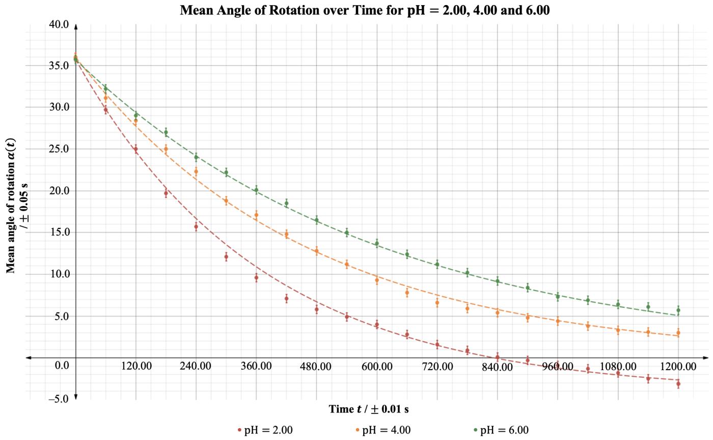
It is evident in Figure 3 that regardless of the pH, the rotation angle of the mixture decays exponentially over time. This was expected as the angle of rotation is given by an exponential function, and all values of �� are negative in the equation below: ��(��)= ��������([������������������]�� [��+]��)��

Comparing the rate constants for the three pH levels, it was found that the pH= 6.00 trials had the least negative value of ��, followed by the pH= 4.00 trials and ultimately the pH= 2.00 trials had the most negative constant. This trend is evidenced as the fastest change of the mean angle of rotation for pH= 2.00 and the slowest change for pH= 6.00. As all experiments started from approximately identical initial rotation angles, and the inversion of sucrose reaction involved the same amounts of reactants, it can be extrapolated that all curves should approach the same horizontal asymptote as �� →∞; due to time constraints, this investigation only took observations up to �� = 1200.00 s.

Conclusion and Evaluation

Conclusion

In conclusion, the investigation hypothesis was that increasing the pH, by increasing the concentration of HCOONa, would result in a less negative rate constant �� for the inversion of sucrose. As evidenced in Figure 3, the reaction of sucrose in a pH= 2.00 buffer solution yielded the most negative rate constant, which in turn indicates the fastest rate of reaction. In contrast, the reaction of sucrose in a pH= 6.00 methanoic acid buffer solution yielded the least negative value of ��, corresponding to the slowest rate of reaction. Hence, the experimental evidence suggests that the original hypothesis may be accepted. The pH= 2.00 buffer solution consisted of 0.570 mol dm 3 methanoic acid. Adding HCOONa to the pH= 2.00 buffer solution disturbs the position of the chemical equilibrium, as the concentration of the conjugate base (HCOO ) increases, and according to Le Chatelier’s principle, the position of the new equilibrium will be established to favour the reactants. By carefully calculating the amount of conjugate base that must be added, solutions with pH= 4.00 and 6.00 were obtained, both of which are less acidic than the original solution due to the common ion effect. The concentration of the acid present directly affects the rate of reaction of the inversion of sucrose, as H+ is

amongst the reactants in this reaction. As the hydrolysis reaction progresses, the dextrorotatory sucrose is turned into a levorotatory solution of glucose and fructose In order to test the hypothesis, it was necessary to gauge the concentration changes over time for the three pH levels; thus, the angle of rotation was recorded over 20 minutes. As the reaction progressed, the angle observed in the polarimeter would gradually become more negative, as more products are generated.

It is common to use polarimetry in order to study reaction kinetics, including the rate of reaction for reactions where the reactant and product solutions demonstrate optical activity. The inversion of sucrose is in fact a well studied reaction with polarimetry (Wienen & Shallenberger, 1988), (Makwakwa, 2014). Accurately modelling the rate of reaction of sucrose inversion is critical in the food industry as establishing the degree of hydrolysis affects the sweetness of sugar and the potential formation of syrup crystals (Sale & Skinner, 1922).

Evaluation

Determiningthevalidityof thisinvestigationinvolves assessingthechoiceoftheindependent(pH),dependent (rate constant) and controlled variables, as well as the experimental methodology. Using pH as the independent variable is a valid choice as its magnitude affects the [H+], which in turn affects the rate constant. The chosen intervals of pH should produce significantly different values of ��, and hence they were designed to be sufficiently apart from one another. The dependent variable (rate constant) is an equally valid choice as it allows to directly test the hypothesis. Since the rate constant depends on the rate of change of the concentrations of all species in the inversion reaction, and concentrations are determinant of the rotation angle of the solution, measuring the angle of rotation over time is a valid methodological process. Furthermore, for the experiment to be valid, appropriate measures were taken to eliminate the effect of the controlled variables on the rate constant, as shown in Table 3

The assumptions for calculating �� with the integrated rate law were that the [H2O] remains constant, and that the [C12H22O11] and [H+] are considered first order and are unequal. In the context of this experiment, these are valid and necessary assumptions as otherwise, the mathematical complexity would be extremely high. Additionally, when preparing the mixture of sucrose and the buffer, it was assumed that the inversion process does not start until the mixture is inserted into the polarimeter, and that the H+ runs out some time after the measurements have stopped. Finally, the angle of rotation of the optically active mixture was calculated assuming that the products of the inversion reaction consisted of a single glucose and a single fructose stereoisomer, produced in a 1:1 molar ratio, which was an essential if not valid assumption.

The reliability of the results was high as the angles of rotation observed for different trials of the same pH were within a narrow range, as detailed in Table 7. For each of the five trials, a pH probe was used to confirm the [H+] was constant, rendering the experiment reliable.

The glassware used for volumetric preparation and sampling of the reactants was as precise as possible in the context of a school laboratory. The electronic balance and pH meter were both highly precise, digital instruments, that could measure masses of 0.001 g and pH of 0.01 respectively. On the other hand, the polarimeter’s precision was lower (±0.5°). This issue becomes more relevant as the sucrose inversion progresses and the rotation angle changes by a progressively smaller magnitude. Due to the cost and sophisticated nature of polarimeters, this experiment relied on the only polarimeter model that was available in this context. Regardless, the value of �� was calculated with a precision of 4 decimal places to illustrate its variability over time. Whilst the polarimeter precision could be higher, the overall precision is acceptable. The results of an accurate experiment would be closely matching the theoretical results; however, the rate constant may not be obtained by simply using a deterministic formula and hence it is challenging to directly compare experimental and theoretical values. As this experiment is very original, the percentage error cannot be calculated, but the accuracy may still be assessed with the help of secondary sources Similar experiments indicated that the rate constant of the sucrose inversion lied within the experimental range of 0.0100 to 0.0450 mol 1 dm3 s 1 and the reaction in a more acidic environment demonstrated a more negative �� (Jenkins & Williams, 1996). In light of the agreement of the experimental and secondary trends, the accuracy can be deemed fairly high.

Table 9 details all sources of error which may have affected the investigation results.

Table 9: Summary of error sources, their significance, and suggested improvements. Source of error Significance and impact of error Improvement to reduce error Systematic errors (which may affect accuracy)

Assuming that the order of sucrose and H+ used to calculate the rate constant is 1 for each reactant.

If the real order of reactants is not 1, the formula used to calculate ��(��) would change. The concentrations used to prepare the solutions of the incremental pH would also be different. Highly significant.

Obtain primary data for the orders of the reactants by designing a reaction kinetics experiment.

Conduct more comprehensive secondary research to seek for more accurate order values and rate law formulas.

Delayed reaction time between the point when the reaction begins and when the first polarimeter measurement is taken (ie. for transferring the solution into the polarimeter and taking the initial measurement).

The H+ may have run out within the 1200.00 seconds that results were being taken.

Assuming that the glucose and fructose in the products each consist of only one stereoisomer, in the molar ratio 1:1.

Observer error when handling the polarimeter to record the value of ��(��) at a specific point in time. The manual operation of the polarimeter induces random errors when discerning the point where the field of view is uniformly coloured yellow.

Inconsistent timing when recording the angle of rotation as the manual process takes a few (2 5) seconds to complete.

Preparation of reactants and the prescribed concentration value may be slightly off.

All values of �� in the experimental data were offset by a constant delay, which in turn would have an impact on the parameters of the exponential decay used in finding ��: ��(��) =��������([������������������]�� [��+]��)��

Relatively significant.

If H+ is no longer present as a reactant in the sucrose inversion, the rate of the reaction would slow down, affecting the value and accuracy of �� Relatively significant

Add the necessary extra steps to the method that would allow measuring the delay time and using that as an offset added to the recorded time intervals. Estimate the value of ��0 by extrapolating the graph.

For every trial, ensure that the sucrose concentration is equal to the H+ concentration, so that both reactants are consumed at the same rate

Obtain a more accurate prediction about the types and ratios of stereoisomers under specific experimental conditions. Adjust the method so that the prescribed reaction conditions are met. Random errors (which may affect precision)

The actual types and ratios of stereoisomers in the products affect horizontal asymptote on the ��(��) graph. This affects the value and accuracy of �� Relatively significant

Qualitatively assessing the colour by eye is inherently random, which may yield erroneous values for the angle of rotation. Highly significant.

The ��(��) values used to plot and analyse the data may have been taken too early or too late in relation to the expected time. Relatively insignificant; ��(��) does not notably change within the delay duration.

The method relied on using specific masses and concentrations of various chemical species. Any random deviation may alter results. Relatively insignificant due to the high precision of the apparatus.

Use a digital or automatic polarimeter with the capacity to display on a screen and potentially extract the ��(��) values to a spreadsheet. This would eliminate the human error in determining the angle of rotation and lead to more accurate and precise results.

Use more precise apparatus to prepare the reactants and use volumetric methods (such as titration) to confirm the exact prescribed concentrations.

Investigation Extension and Improvements

Given enough time, the experimental process could have been altered to test multiple pH levels in shorter intervals (for instance pH= 1.00, 1.50, 2.00, etc.). This would improve the evaluation of the hypothesis that the angle of rotation is affected by the pH levels. Furthermore, the modifications proposed in Table 9 could be implemented without changing the aim and overall direction of the experiment. A possible extension of the experiment would be to introduce a range of new qualitative and quantitative experimental considerations or parameters, such as texture and taste of the invert sugar and the costs of preparation in an industrial setting This would ensure that a more practical interpretation of the results could be made, as the angle of rotation itself has little relevance in the industrial preparation of food. Rather, the angle of rotation could be paired with these additional factors as an indicator of the optimal pH and time (of inversion) to produce the sweetest, commercially favourable invert sugar. This would require an extended methodology with further steps designed to determine the effects of changing pH on the effectiveness of the invert sugar as a sweetener and preservative, as well as the usefulness of polarimetry in commercial applications.

Reference List

Anton Paar GmbH. (2021). Sugar inversion. Anton Paar. https://wiki.anton paar.com/en/sugar inversion/#why worry about sugar inversion Bora, K. J., Goswami, D., Upadhyay, V., & Kalita, D. (2018). Optical method for measuring optical rotation angle and refractive index of chiral solution. Bulletin of Physics Projects, 3, 27 31. https://www.bbcphysics.in/images/pdfs/BPP Vol 3_pdf/article 5.pdf

Boundless Learning. (n.d.). The Integrated Rate Law. Lumen. Retrieved February 6, 2021, from https://courses.lumenlearning.com/introchem/chapter/the integrated rate law/ Brown, C., & Ford, M. (2014). Higher Level Chemistry (2nd ed.). Pearson Education. Clark, J., Danai, M., Tung, E., & Chieh, C. (2019). Common Ion Effect. Chemistry LibreTexts. https://chem.libretexts.org/Bookshelves/Physical_and_Theoretical_Chemistry_Textbook_Maps/Sup plemental_Modules_(Physical_and_Theoretical_Chemistry)/Equilibria/Solubilty/Common_Ion_Effe ct

Harned, H. S., & Embree, N. D. (1934). The Ionization Constant of Formic Acid from 0 to 60°. Journal of the American Chemical Society, 56(5), 1042 1044. https://doi.org/10.1021/ja01320a010

Jenkins, B., & Williams, J. (1996, November 6). Inversion of sucrose; kinetics of a pseudo first order reaction determined by polarimetry differential equations. http://people.uncw.edu/lugo/MCP/DIFF_EQ/deproj/sucrose/sucrose.htm

Makwakwa, T. A. (2014). A Study of the Effect of Salt Solutions on the Kinetics of Sucrose Inversion as Monitored by Polarimetry. University of South Africa. http://uir.unisa.ac.za/bitstream/handle/10500/18902/dissertation_makwakwa_ta.pdf;sequence=3

NSW Education Standards Authority. (n.d.). Formic Acid. Chemical Safety in Schools. https://online.det.nsw.edu.au/ecmjsp/chemicals/?mode=viewchemares&chemalpha=F&chemid=795 #skipToContent

Physical Chemistry Laboratory. (2018). Chemical Physics | Details. Tel Aviv University. https://www.tau.ac.il/~phchlab/exp inversion theory.html

Sale, J. W., & Skinner, W. W. (1922). Relative Sweetness of Invert Sugar. Journal of Industrial & Engineering Chemistry, 14(6), 522 524. https://doi.org/10.1021/ie50150a019

The Nest Group, Inc. (2016, December 2). Molarity of Concentrated Acids & Bases https://www.nestgrp.com/protocols/trng/molarity.shtml

Wienen, W. J., & Shallenberger, R. S. (1988). Influence of acid and temperature on the rate of inversion of sucrose. Food Chemistry, 29(1), 51 55. https://doi.org/10.1016/0308 8146(88)90075 1

Appendices

Appendix A: ���� calculations (using ICE tables)

Changing the concentration of HCOO in the equilibrium mixture of the reaction leads to a change in pH. An ICE table was used with the concentrations of HCOOH, H+ and HCOO to change the independent variable. Table 10 shows the calculation for a pH of 2.00

Table 10: ICE table for a pH of 2.00.

[HCOOH] [H+] [HCOO ] Initial 0570 0000 0000 Change 00100 00100 00100 Equilibrium 0.560 0.0100 0.0100 pH= log[H+]= log001=200

When the HCOONa is added to a solution of HCOOH at equilibrium, according to Le Chatelier’s principle, the reaction favours the reactants. In turn, this means that an amount of H+ and HCOO ions will react and form methanoic acid. Letting the concentration of this amount be �� mol dm 3 (this is the amount in the “Change” row of Table 11), when equilibrium is established, the ���� can be expressed as: ���� = [H+][HCOO ]

[HCOOH] 1.77×10 4 = (001 ��)(�� ��) 0560+�� where �� = concentration of HCOONa required, in order to achieve pH of 4.00 in the buffer solution. The solution to this equation was approximated with the software Wolfram Alpha and it was found to be equal to: �� =5×10 7 ×(1000000�� √1000000000000��2 19646000000��+500051329+10177) In order for the pH to be approximately 4.00, the [H+] at equilibrium (0.01 ��) must be equal to 100×10 4. Hence, using the solver feature in Excel, it was calculated that �� must be 0700 mol dm 3 Table 11: ICE table for a pH of 4.00. [HCOOH] [H+] [HCOO ] Initial 0.560 0.0100 0.700 Change 9.85×10 3 9.85×10 3 9.85×10 3 Equilibrium 0.570 1.02×10 4 0.690 pH= log[H+]= log(102×10 4)=399≈400 The calculation for pH of 6.00 was conducted in a similar manner.

Appendix B: Stoichiometric calculations used in the method Other relevant calculations used for the stoichiometric relationships in the method are evident in Table 12 Table 12: Stoichiometric calculations used in the method. Calculation for the dilution of the methanoic acid solution (in step 2 of the method).

Calculation for mass of sucrose used (in step 4 of the method).

��1��1 =��2��2 ��2 = 23.6×0.100 0.570 =41403508772≈414dm3

��= ���� ��= ������ The volume used is 0.0100 dm3, due to the maximum volume which can be input in the polarimeter’s observation tube. Arbitrarily assuming a concentration of C12H22O11 of 0.100 mol dm 3: ��= 0100×00100×(12×1201+22×101+11×1600) ��= 0.342g

Calculation for amount of HCOONa added when pH= 4.00 (in step 10 of the method).

Calculation for amount of HCOONa added when pH= 6.00 (in step 14 of the method).

��= ������

The volume used is 0.0100 dm3, due to the maximum volume which can be input in the polarimeter’s observation tube. According to Le Chatelier’s principle, a concentration of 0.710 mol dm 3 of HCOONa is required for an equilibrium pH of 4.00:

��= 0700×00100×(101+1201+2×1600+2299)

��= 0476g

��= ������

The volume used is 0.0100 dm3, due to the maximum volume which can be input in the polarimeter’s observation tube. According to Le Chatelier’s principle, a concentration of 2.223 mol dm 3 of HCOONa is required for an equilibrium pH of 6.00: ��= 2.213×0.01×(1.01+12.01+2×16.00+22.99) ��= 1.505g

Appendix C: Sample calculations for the uncertainty of the initial concentrations of sucrose and H+, and the rate constant ��

Table 13 includes the calculations for the uncertainty of [C12H22O11]0 for all trials, and a sample calculation for the uncertainty of [H+]0 for all pH= 2.00 trials.

Table 13: Sample calculations for initial concentrations uncertainties. Uncertainty of [C12H22O11]0 for all trials: Uncertainty of [H+]0 for all pH= 2.00 trials: �� = �� �� = �� ���� since �� is a constant, it has no uncertainty

percentageuncertainty = 0.001 0.342 ×100+ 0.05 10 ×100 =0.79% uncertainty = 0.79 100 ×0.01=±7.9×10 5 moldm 3

To find this uncertainty, an indirect method was used as there is no direct calculation for the propagation of uncertainties of exponential functions. Namely, the extreme values of [H+]0 were calculated, and the uncertainty was found as: [H+]0 =10 pH [H+]0lowerboundary = 10 200 001 = 9.772×10 3 [H+]0upperboundary = 10 200+001 =1.023×10 2

uncertainty =max(|[H+]0upperboundary [H+]0|, |[H+]0lowerboundary [H+]0|) =max(23×10 4,228×10 4) =±2.3×10 4 moldm 3

Please note that the value of the uncertainty ends up being the same for all pH= 4.00 and 6.00 trials as well.

Finally, Table 14 explains the uncertainty calculation for the rate constant for pH= 2.00 at �� = 60.00 s.

Table 14: Sample uncertainty calculation for the rate constant. Uncertainty for the rate constant for pH= 2.00 at �� = 60.00 s: �� =

ln(��(��) ��0 ) ([C12H22O11]0 [H+]0)��

For the numerator, a similar process was used as with the exponential function in Table 13. ln(��(��) ��0 ) lowerboundary =ln([297 05] [35.9+0.5])= 0.2204

For the denominator, the uncertainty for the concentration difference and the time had to both be found: uncertaintyofconcentrationdifference =2.3×10 4 +7.9×10 5 =3.09×10 4 moldm 3

ln(��(��) ��0 ) upperboundary = ln([29.7+0.5] [35.9 0.5])= 0159

uncertainty =max(|ln(��(��) ��0 ) upperboundary ln(��(��) ��0 )|, |ln(��(��) ��0 ) lowerboundary ln(��(��) ��0 ) |) =max(0.031,0.031) =±0031

percentageuncertainty = 0031 ln(29.7359) =16.2%

percentageuncertaintyofconcentration difference = 3.09×10 4 01 001 ×100=0.343%

percentageuncertaintyoftime = 0.01 60 ×100= 0.017%

The final uncertainty of �� is hence: percentageuncertainty =105%+0343%+0017%=±1656% uncertainty = 16.56 100 ×00351= ±00058mol 1 dm3 s 1

Investigation of the Effect of Impedance on the Power Factor of an RLC Circuit

Exploration

Research Question

What is the relationship between the impedance (1.00, 2.00, 3.00, 4.00 Ω) and the power factor of an RLC AC circuit, considering capacitive and inductive effects?

Introduction and Rationale

Power transmission and distribution networks deliver electricity from power plants to the consumer via alternating current (AC) circuits (Hamper, 2014). Furthermore, multiple electrical devices, such as motors and conveyor belts, use AC power. Due to the presence of electric and magnetic fields in capacitors and inductors respectively, the delivered power to the load of an AC circuit may be adversely affected. The concept of impedance, which is used to describe the aforementioned effects, is critical to investigate the delivered power in an AC circuit.

After studying capacitance in class in relatively simple circuits, my curiosity and interest in the topic enabled me to begin further research into more complex circuits involving capacitors, such as RLC circuits. Personally, I was extremely fascinated by the factors which affect power loss, seeing the great importance of AC power in numerous aspects of our daily lives. This investigation enabled me to understand the ways in which power loss can be minimised, which can in turn contribute to improved efficiency and sustainability in industrial and distribution settings. Electrical engineering is also a career path that I am considering after school, and hence this experiment acts as an indicator of what I can expect to study in the future.

Background

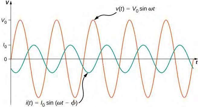
Most AC circuits contain resistors, capacitors and inductors; they are referred to as RLC circuits . The angular frequency (�) of an AC circuit characterises how rapidly the voltage and current change polarity and is proportional to the frequency as per � = 2�� (Ling et al., 2016). Both the voltage and the current in such a circuit change in a sinusoidal manner as seen in Figure 1, according to the equations: � (�) = �0 sin �� � (�) = �0 sin(�� � )

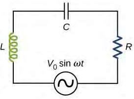
There is a phase difference (� ), measured in radians, between the voltage and current curves which depends on the inductance (� ) and capacitance (� ) of the circuit. Capacitance is measured in Farad (F) and inductance is measured in Henry (H). Capacitors in RLC circuits charge and discharge continuously, which results in the presence of electric fields between the two metal plates. These electric fields oppose changes in current, an effect that is described with the quantity known as capacitive reactance (�� ). Similarly, RLC circuits contain inductors, which demonstrate an opposition to the flow of current via the induction of magnetic fields (Hewes, 2007). This effect is described as inductive reactance (�� ). Both reactances depend on � and the respective parameters of the capacitor (� ) and inductor (� ), and are measured in Ohms (Ω).

Figure 1: The schematic of an RLC circuit (left) and the changes in voltage and current over time (right) ; (Ling et al., 2016)

Collectively, the effects of opposing the current due to the reactances and the effect of voltage drop as a result of resistance (� ) are described by the quantity known as impedance (�)

� = √� 2 + (�� �� )2

While the resistance and the reactances have the same dimensions, they are not added algebraically, implying that they have a more complex geometrical relationship between them. In fact, t hey are all represented by vectors, where the � , �� and �� describe the magnitudes (Ling et al., 2016). However, each of the � , �� and �� have different effects on the phase angle � , specifically:

• The resistance does not cause a phase difference (� = 0).

• The capacitive reactance generates a phase difference of � = � 2 . This results in the current leading the voltage by � 2

• The inductive reactance generates a phase difference of � = + � 2 . This results in the current lagging the voltage by � 2

Depending on the relative magnitudes of the capacitive and inductive reactances, RLC circuits are classified as capacitive (when �� > �� ) or inductive (when �� < �� ). In a similar fashion to the reactances, there are three different components of the voltage in an RLC circuit: �� , �� and �� . The voltage components, along with the current, are typically drawn in phasor diagrams, where all vectors rotate about the origin and by convention the current vector is drawn parallel to �� . A phasor diagram for an RLC circuit is depicted in Figure 2.

The resistance (� ) and reactance ( �� and �� ) phasors are always in phase with their respective voltages. The phase angle � may be calculated using trigonometry as seen in Figure 2.

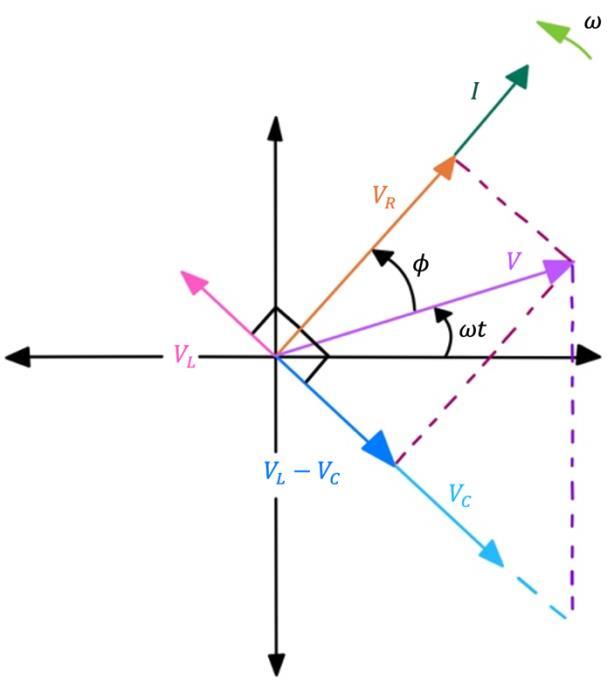
�=arctan(�� −�� �� )=arctan(�� −�� � )

It follows that if �� ≠�� , then the phase angle �≠0 In this scenario, the power dissipated in an AC circuit has two natures: real power (� ) and reactive power (� ). The real power (� ) represents the actual amount of power being consumed in the circuit. As with DC circuits, it is measured in Watts ( W). On the other hand, reactive power (� ) is the amount of power stored momentarily in electric and magnetic fields in the capacitors and inductors respectively. It is measured in Volt Amperes reactive (VAr), which is a unit that represents the same amount of power as 1 W (Ling et al., 2016).

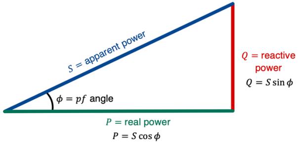
Figure 2: Phasor diagram of an RLC circuit.

For inductors and capacitors, due to the phase difference between the voltage and the current, there are times where the voltage and the current have opposite signs. Power flowing in an inductor or capacitor is calculated as the product of voltage and current ( � (�) = � (�) �(�)). Half of the time, � (�) and � (�) will have the same sign; hence, the power would be positive. Accordingly, for the other half of the time, the power would be negative as �(�) and � (�) have opposite signs. When the power is positive, the inductors and capacitors both store energy from the circuit; when the power is negative, they both release energy back into the circuit. Hence, on average, the capacitive and inductive devices have a net zero power dissipation in AC circuits.

An AC circuit must be able to handle both the real and reactive power at any point in time in order to avoid burning or damaging the circuit. The combined eff ect of real and reactive power is called apparent power ( �) and is calculated as the geometric sum of its components using Pythagoras’ theorem, as illustrated in Figure 3 (Kuphaldt, 2020).

� = √� 2 + �2

Figure 3: Geometric sum of the apparent power.

The SI unit for apparent power is Volt Amperes (VA). The equivalent AC calculation, derived from Ohm’s law, for the power dissipated in a DC circuit with resistor s (� = � 2 �) is: � = � 2 �

The ratio of real power to apparent power (or resistance to impedance) is equal to the power factor ( �� ): �� = cos � = � � = � � = � √� 2 + (�� �� )2

The power factor is a very useful metric that represents the utilisation of power in an AC circuit. The closer it is to 1, the lower the reactive power, which in turn means the real power is transferred to the load more efficiently.

Hypothesis

The maximum power factor of an RLC AC circuit will be observed when the inductive reactance is equal to the capacitive reactance, and thus the impedance is equal to the resistance. This is inferred from the fact that when �� = �� , � = 0, and hence cos � is at its maximum value of 1. Whenever �� > �� (circuit is inductive in nature), it should be that � > 0 and whenever �� < �� (circuit is capacitive in nature), it should be that � < 0 As long as the phase angle is between � 2 to � 2 , the power factor ( cos � ) will be between 0 and 1. The power factor of the circuit pairs with equal magnitude impedance values is expected to be also equal.

Methodology

Variables

The independent variable is elaborated on in Table 1

Table 1: Independent variable Independent variable Variation method

Impedance ( � )

Use seven different RLC circuits, designed appropriately to ensure that each circuit gives a different value for the impedance.

Impedance increments and nature

4.00 Ω, capacitive 3.00 Ω, capacitive 2.00 Ω, capacitive 1.00 Ω, neither capacitive nor inductive 2.00 Ω, inductive 3.00 Ω, inductive 4.00 Ω, inductive

In this experiment, six circuits (three capacitive and three inductive) were tested along with another circuit which was neither capacitive nor inductive. The rationale behind this design decision was threefold. Firstly, it allows for testing the hypothesis, where the circuit which is neither capacitive nor inductive is expected to have the highest power factor. Moreover, investigating both capacitive and inductive RLC circuits to vary impedance is more pertinent to real life engineering and physics systems (Qabazard, 2015). Finally, it allows for determining whether the power factor variation in capacitive or inductive RLC circuits is symmetrical

The first step in the circuit design was the choice of the resistance value. The value of � should be relative ly small in order for the reactances to be of comparable magnitudes and to be able to purchase appropriate capacitors and inductors that are commonly available (which usually have a small capacitance and inductance respectively). The value of � was arbitrarily chosen to be 1.00 Ω. Next, the angular frequency of the circuit was calculated as � = 2�� = 2� × 50 ≈ 314 rad. s 1. Beginning from the circuit with impedance 1.00 Ω, which has �� = �� , it follows that �� = 1 �� , and hence �� = 1 � 2 ≈ 1 01 × 10 5 . By arbitrarily choosing the value of � = 1.00 × 10 3 F, it can be calculated that the value of � must be approximately 1.00 × 10 2 H. Hence, the impedance of the circuit with a 1.00 Ω resistor, a 1.00 × 10 3 F capacitor and a 1.00 × 10 2 H inductor is: �

Starting from this base circuit, three more capacitive and three more inductive RLC circuits were designed so that the impedance varied by 1.00 Ω each time. For the capacitive circuits, the inductance was arbit rarily chosen to be very small ( 1.00 × 10 6 H) so that �� < �� . Accordingly, for the inductive circuits, the capacitance was arbitrarily chosen to be relatively high ( 1.00 × 10 2 F) so that �� > �� . For each of these six circuits, the target impedance, angular frequency, resistance and one of � or � were known, and thus it was possible to calculate the necessary � or � value respectively. For example, in order to design the capacitive RLC circuit with an impedance 2.00 Ω: � = √� 2 + (�� �� )2 = √� 2 + (�� 1 �� )2 ∴ � = | 1 � 2 � �√� 2 � 2 | � = | 1 3142 × 10 6 314√22 12 | ≈ 1 80 × 10 3 F

This process was repeated for the five additional circuits in order to achieve impedances of 2.00, 3.00 and 4.00 Ω in inductive and capacitive nature, as summarised in Table 2 The experimental impedances are slightly off from the originally planned 1.00 Ω intervals. This limitation was imposed due to the availability of specific values of capacitance and inductance in the market components.

Table 2: Circuit design and parametrisation summary Circuit number Capacitance / F Inductance / H Capacitive reactance / Ω Inductive reactance / Ω Impedance / Ω Circuit Nature

1 8.20 × 10−4 1.00 × 10−6 3.88 3.14 × 10−4 4.01 Capacitive

2 1.13 × 10−3 1.00 × 10−6 2.82 3.14 × 10−4 2.99 Capacitive

3 1.80 × 10−3 1.00 × 10−6 1.77 3.14 × 10−4 2.03 Capacitive

4 1.00 × 10−3 1.00 × 10−2 3.18 3.14 1.00 Neither

5 1.00 × 10−2 6.50 × 10−3 0.32 2.04 1.99 Inductive

6 1.00 × 10−2 1.00 × 10−2 0.32 3.14 3.00 Inductive

7 1.00 × 10−2 1.33 × 10−2 0.32 4.18 3.99 Inductive

Table 3 explains the dependent variable.

Table 3: Dependent variable Dependent variable Measurement method

Power factor ( �� )

The power factor (�� ) will be calculated as cos � , where � is the phase angle obtained by comparing the source AC voltage as compared to the RLC alternating voltage curves.

Justification Units

Using school equipment, the most direct way to obtaining the power factor is by determining the phase angle for each value of the impedance. The phase angle itself is directly related to impedance, according to:

This is a dimensionless quantity (no units).

Table 4 details all of the controlled variables in this experiment.

Table 4: Controlled variables

Controlled variable Control method

Ambient temperature kept at 25ºC (room temperature).

Carry out all trials in the same airconditioned laboratory.

Justification

The resistance, capacitance and inductance values are affected by temperature. If the temperature was not controlled, the impedance calculation would be invalid (Li & Yin, 2017). Minor fluctuations are negligible.

Same pieces of electrical equipment used in all trials of the same circuit.

Oscilloscope model and setting.

Use the same type of resistors, capacitors, inductors, connecting wires and breadboards for each circuit.

Use the exact same oscilloscope for every trial of every circuit, configured in the same way.

This warrants that the only factor affecting the dependent variable across the different trials for each circuit is the impedance. If different types of electrical equipment were to be used in each trial, there is a higher risk of the impedance value being affected due to discrepancies in the manufacturer’s tolerance.

To ensure the measurements for the phase angle and impedance are made with the same instrument (and same configuration).

Resistance �= 1.00 Ω

The load resistor in all circuits is of equal resistance ( �= 1.00 Ω) and same model (same company).

This investigation aims to determine the effect of impedance, in capacitive and inductive RLC circuits, on the power factor. Varying resistance would affect the overall impedance (and hence the power factor), as well as the capacitive or inductive nature of each circuit.

2.00 V output used in all circuits.

Do not alter the voltage setting on the power pack for any trial; keep it at 2.00 V.

The oscilloscope has a vertical scale of 2.00 mV to 10.0 V, meaning that 10.0 V is the maximum potential difference which can be used in this experiment. 2.00 V was arbitrarily chosen as a relatively small voltage would justify the use of small resistance and reactance values; the smallest power pack output available was 2.00 V.

The resistance ( � ) and reactance ( �� and �� ) phasors remain in phase with their corresponding voltages, �� , �� and �� . Changing the voltage would affect the value of � and therefore the power factor for all impedances.

Frequency maintained at 50.0 Hz.

Risk Assessment

Use the same power pack in each circuit for all trials.

The frequency must be kept constant so that � is also a constant value. If � varied, it would affect the capacitive and inductive reactances and therefore the impedance.

Table 5 details hazards, risks posed and mitigations to establish a safe experimental environment.

Table 5: Risk assessment.

Hazard Risk posed Mitigation

The risk of an electric shock can arise due to the one of the following reasons:

1.Using unsafe or defective electrical components.

Each risk posed can be minimised by:

Risk of electric shock.

2.Electrical conductors come in contact with wet hands.

3.Touching any exposed wires or any energised, uninsulated component. These may cause skin burns, or even internal tissue and heart damage under certain conditions.

1.Using new capacitors, inductors, resistors and breadboards (which are less likely to be faulty) and visually inspect pre-used equipment to ensure there are no apparent defects.

2.Thoroughly dry hands before handling any electrical equipment and make sure that there is no water near the circuits.

3.Confirm that all cables and devices are securely plugged in. Use latex gloves when handling equipment.

Burns or fire risk if shortcircuited.

Short-circuit may appear due to defective electrical components or incorrect connection in the circuit. The current may reach dangerously high levels, creating a fire hazard and risk of burns or electric shock.

Only work with the components with the power pack disconnected and off. Confirm that all cables and devices are securely plugged in and use well-insulated wires. Use latex gloves and identify the location of the first aid kit and fire extinguisher in the laboratory.

Dropping the oscilloscope or power pack on the ground.

Equipment

The oscilloscope and power pack (each having a mass of a few kg) are quite heavy and may result in broken bones or other injuries if it falls on someone. It can also fall on the ground where someone may trip over it, or may cause structural damage.

Place the oscilloscope and power pack away from the edge of the laboratory bench and ensure that only the experimenter is near the devices. Neatly collect any loose hanging wires to mitigate trip hazard.

The required components for this experiment are shown in Table 6

Table 6: Equipment list.

Quantity Equipment

1 100 MHz digital storage oscilloscope (PASCO SB 9621A)

Uncertainty

± 0.5 ms

1 50.0 Hz Battery pack (IEC LB2631-101) ± 0.10 Hz

1 pair Latex disposable gloves

2 Connector wires

2 Alligator clips

3 1.00 × 10−2 F, 10V capacitors (CDE/Illinois 109TTA010M) ±20%

1 1.80 × 10−3 F, 40V capacitor (KEMET PEG225KG4180ME1) ±20%

2 1.00 × 10−3 F, 16V capacitors (Vishay MAL212015102E3) ±20%

1 1.30 × 10−4 F, 250V capacitor (Vishay 53D131F250HJ6) 10%, + 50%

1 8.20 × 10−4 F, 40V capacitor (Vishay MAL212517821E3) ±20%

1 4.70 × 10−3 H, 55 mA inductor (EPCOS/TDK B78108S1475J) ±5%

1 1.80 × 10−3 H, 95 mA inductor (EPCOS/TDK B78108S1185J000) ±5%

3 1.00 × 10−2 H, 0.06 A axial inductors (EPCOS/TDK B82144A2106J) ±5%

1 3.30 × 10−3 H, 62 mA inductor (EPCOS/TDK B78108S1335J) ±5%

3 1.00 × 10−6 H, 2.2 A inductor (EPCOS/TDK B82144A2102K) ±10%

7 1.00 Ω metal oxide resistors (KOA Speer MOSX2CT52A1R0J) ±5%

7 Half-size breadboard (Digilent 240-131)

Method

Part A: Circuit design (for the specific electrical circuit diagrams , refer to Appendix B).

1. Connect one 1.00 Ω resistor in each one of the seven breadboards. 2. Connect the capacitor and inductor and shown in Table 7 for circuit 1 in series to the resistor. 3. Repeat step 2 for circuits 2 7 on a separate breadboard. For circuit 2, the two capacitors must be connected in parallel to each other, and for circuits 5 and 7, the two inductors must be connected in series.

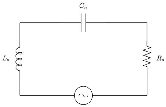
Table 7: List of components for each circuit.

Circuit List of capacitors

List of inductors

1 one 8.20 × 10−4 F one 1.00 × 10−6 H 2 one 1.00 × 10−3 F one 1.00 × 10−6 H one 1.30× 10−4 F 3 one 1.80 × 10−3 F one 1.00 × 10−6 H 4 one 1.00 × 10−3 F one 1.00 × 10−2 H 5 one 1.00 × 10−2 F one 4.70 × 10−3 H one 1.80 × 10−3 H 6 one 1.00 × 10−2 F one 1.00 × 10−2 H 7 one 1.00 × 10−2 F one 1.00 × 10−2 H one 3.30 × 10−3 H

Part B: Data collection

Figure 4: Generic electrical diagram showing the RLC circuits.

1. Connect the power pack to the two holes of the breadboard at the beginning and end of the RLC circuit 1. 2. Connect the ground and channel 1 probes of the oscilloscope across the 1.00 Ω resistor. 3. Connect the channel 2 probe of the oscilloscope at the point between the inductor and the power pack.

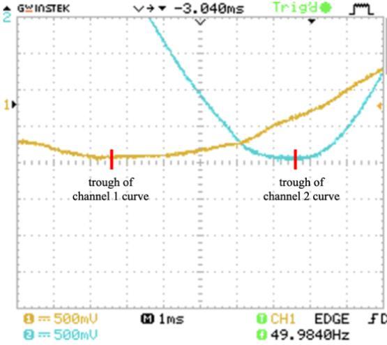
4. Turn on the power at 2.00 V and 50.0 Hz and adjust the vertical position of each curve so that the troughs (minimums) of the sinusoidal graphs lie on the horizontal axis . Also, adjust the horizontal scale of the oscilloscope so that appropriate phase difference measurements may be obtained

5. Record the phase difference ( ∆� ) between the two sinusoidal waveforms in the oscilloscope screen as the horizontal displacement between the two troughs.

6. Repeat steps 2 5 another four times.

7. Repeat steps 1 6 using RLC circuits 2 to 7.

Results and Analysis

Raw Data

Qualitative Data

When the oscilloscope probes were connected at the ind icated points in each circuit, the screen displayed two sinusoidal curves corresponding to the voltage at each probe. The characteristics of the sinusoidal curves changed according to the variation in the value of impedance (amplitude and phase difference) . An example showing the phase difference is evident in Figure 5.

Quantitative Data

Quantitative raw data collected is sh own in Table 8. Please note that during the data processing, the impedance magnitude was assumed to have no uncertainty. This was a necessary assumption as otherwise, according to the manufacturer tolerance values, the final uncertainty would be unreasonably large. An example of the aforementioned issue, and the relevant calculations, can be found in Appendix A

Table 8: Quantitative raw data

Impedance (

Figure 5: Oscilloscope screenshot showing the phase difference between the two voltage curves in circuit 7.

Data Processing

A summary of all processed data is evident in Table 9

Table 9: Summary of processed data

Circuit Average phase difference / ±0.0005 s

Average phase angle � / ±0.03 rad)

Power factor �� 1 0.0250 1.25 0.315 ± 0.029 2 0.0230 1.15 0.408 ± 0.028 3 0.0210 1.05 0.498 ± 0.026 4 0.0000 0.00 1.000 ± 0.000 5 0.0210 1.05 0.498 ± 0.026 6 0.0230 1.15 0.408 ± 0.028 7 0.0250 1.25 0.315 ± 0.029

For circuit 4, the uncertainty for the phase angle was assumed to be ± 0.03 rad, as calculating with ∆� � would result in a division by 0. Furthermore, the uncertainty in phase angle of ± 0.03 rad would result in �� with a value of 1.000 for both the upper and lower boundaries. This is a result of the nature of the cosine function, where cos ( 0.03) = cos (0.03).

The average phase difference for each trial was calculated as follows:

Average phase difference for circuit 1:

∆� = 25.0+ 25.0+ 25.0+ 25.0+ 25.0 5 ∆� = 25.0 ms ∆� =0.0250 s

uncertainty= 0.5+0.5+0.5+0.5+0.5 5 uncertainty =±0.5 ms uncertainty =±0.0005 s

As explained earlier, the phase angle is illustrated as the horizontal displacement of the two curves in relation to one another. The oscilloscope’s horizontal axis has dimensions of time, whilst the phase difference has dimensions of angle. Hence the measure ments must be normalised by dividing by the period � . Furthermore, since � = 1 � , and the frequency in the experiments is always 50 .0 Hz, � and �� may be calculated as: � (rad) = ∆� � = � ∆� = 50 0∆� �� = cos �

Average phase angle for circuit 1: �=−50.0×0.0250 � =−1.25 rad uncertainty=(0.01 50.0 + 0.0005 0.0250)× 100 =2.02% uncertainty = 2.02 100 × |−1.25| =0.02525 ≈±0.03

Average power factor for circuit 1: �� = cos(−1.25) �� =0.315

��lower boundary = cos (−1.28) =0.286 ��upper boundary = cos (−1.22) =0.343

uncertainty=max(|��upper boundary ��|,|��lower boundary ��|) uncertainty =max(0.029,0.028) uncertainty =±0.029

Figures 6 and 7 are graphs showing the relationship between the power factor the impedance, for circuit s 1 4 and 4 7 respectively.

Relationship between the Power Factor and Impedance (Circuits 1 4)

Power factor

1.000

0.800

0.600

0.400

0.200

0.000

1.200 0.00 0.50 1.00 1.50 2.00 2.50 3.00 3.50 4.00 4.50

Impedance (Ω)

Experimental Values Theoretical Values

Figure 6: Graph showing the dependence of the power factor on impedance for the capacitive circuits. Please note that the circuit with impedance 1.00 Ω is neither inductive nor capacitive.

Relationship between the Power Factor and Impedance (Circuits 4 -7)

Power factor

1.000

0.800

0.600

0.400

0.200

0.000

1.200 0.00 0.50 1.00 1.50 2.00 2.50 3.00 3.50 4.00 4.50

Impedance (Ω)

Experimental Values Theoretical Values

Figure 7: Graph showing the dependence of the power factor on impedance for the inductive circuits. Please note that the circuit with impedance 1.00 Ω is neither inductive nor capacitive.

In Figures 6 and 7, it is evident that the power factor has an inversely proportional relationship to the impedance. This trend was expected as the power factor is given by (as explained in the Background Information) �� = � � . The trend shows a purely resistive AC circuit (circuit 4, as �� = �� ) has the highest power factor. On the contrary, the circuits with most dominant capacitive (circuit 1) or inductive (circuit 7) nature demonstrated the lowest power factor.

Conclusion and Evaluation

Conclusion

To conclude, in this experiment the following hypothesis was tested: when the inductive reactance was of the same magnitude as the capacitive reactance, the power factor of the RLC AC was expected to be at a maximum. After the seven circuits were tested, and the results were processed, it was evident that the highest power factor was observed when �� = �� . In turn, the phase difference between the voltage and current in these circuits was 0 ( � = 0), and therefore the power factor ( �� = cos �) obtained its maximum value of 1. Hence, there is evidence to suggest the hypothesis can be accepted. The phenomena responsible for the observed trend can be attributed to the continuous charging and discharging of the capacitors and the induced magnetic fields in the inductors, both of which introduce additional resistance to the flow of current. Thus, in order to minimise losses in electrical power transmission and distribution in AC circuits, the inductive and capacitive effects must cancel out. As the presence of ind uctors and capacitors is unavoidable in most large scale AC circuits, such as power generation and industrial motors, an extensive effort must be applied to ensure that �� = �� . In most modern applications, this is achieved with the help of power electro nics, which continuously monitor the power factor and if it deviates from 1, they dynamically modify �� or �� using a negative feedback architecture (Kundur, 1994).

The secondary hypothesis that could be tested in this experiment was whether the power factor of the circuit pairs with equal magnitude impedance values would be equal. The symmetry of capacitive and inductive effects in circuits with the same magnitude of |�� �� | , but opposite values of � (for instance, circuits 1 and 7), was confirmed by the analysis of experimental results. This implies that regardless of whether there are capacitive or inductive effects in an AC circuit, the power factor experiences a similar drop. Individually, capacitors and inductors may cause significant power losses in AC RC and RL circuits; however, the aforementioned engineered symmetry could be utilised to minimise power losses. The principle used by power electronics to achieve power factors close to 1 in real life applications relies exactly on this circuit design

Evaluation

In assessing the validity of this experiment, the choice of the independent (impedance) and dependent (power factor) variables, the control methods of the controlled variables, and the expe rimental methodology must be considered. In the research hypothesis, it was claimed that the power factor of the RLC circuit would depend on the impedance, and would obtain the maximum value when the impedance was minimum. Choosing the magnitude and nature of the impedance as the independent variable, and the power factor as the dependent variable, rendered the experiment valid. The variation of the independent variable was incremental in intervals of 1.00 Ω, starting from highly capacitive (4.00 Ω) to purely resistive (1.00 Ω) to highly inductive (4.00 Ω). Since both the inductive and capacitive reactances depend on the angular frequency, which is not a conveniently integer number, extensive care was taken when designing each circuit to ensure that the impedance varied according to the 1.00 Ω intervals, as in Tables 2 and 7. Additionally, as shown in Table 4, appropriate measures were taken to ensure that all controlled variables were kept constant , which in turn, further improves the validity Finally, the method steps were designed in a logical order so that all the variations in the impedance would produce a measurable effect on the power factor, and they could be replicated easily by any other researchers in the future without ambiguity.

In assessing the reliability of the investigation, the c onsistency of results must be evaluated . For each circuit configuration, the exact same independent variable values were used as input, and hence a reliable result would produce the same output, as was seen in Table 8 Given that all five phase differences in each circuit were measured to be the same, the reliability of the experiment can be deemed exceptionally high. Furthermore, the pairs of circuits with corresponding impedance magnitude, but opposite phase angles, (circuits 1 and 7; 2 and 6; 3 and 5) produced the exact same phase difference measurements, which confirms the high reliability . The experiment featured measurements done with highly precise, digital equipme nt. Namely, the oscilloscope used was able to measure the phase difference (which was critical to calculating the power factor) with a precision of ±0.0005 s. This ensures the measurements were reliable and precise. On the other hand, with regards to precision, the tolerance provided by the manufacturer for the magnitudes of inductance, capacitance and resistance varied from ±5% to 10%, +50% (as was indicated in Table 6). Inevitably, such high tolerance values introduce the risk of having imprecise impedance in a particular circuit , especially circuit 2, where a high uncertainty capacitor was used However, this is not a factor that can be controlled or mitigated, d ue to the inductors, capacitors and resistors available for purchase. Additionally, there was no evidence of circuit 2 having a higher percentage error compared to its pair circuit 6 (refer to Table 10). During the data processing, the impedance magnitudes were assumed to have no uncertainty, as otherwise the final uncertainty for the power factor would propagate to unreasonably large numbers. Lastly, all measured and processed values were obtained to 3 significant figures, ensuring that the number of decimal places corresponded with the uncertainty of each device. Such level of precision is satisfactory for an investigation of this nature. The accuracy of the experiment may be assessed as the relative difference between the measured power factors and the theoretical power factors , calculated using �� = � � . The mean percentage error for each circuit can be seen in Table 10 All experimental values, with the exception of circuit 5, are overestimates of the theoretical values, which indicates a source of systematic error due to a potential, unconscious observer bias. As illustrated in Figure 5, the apex of both curves, and in particular the channel 1 curve, were exceptionally broad. The process of exporting oscilloscope data directly to a spre adsheet could not be completed due to incompatibility issues (which produced incoherent measurements in the dataset) ; hence the phase difference had to be measured by eye as the horizontal difference between the troughs of the two curves The broadness of the curves rendered an accurate measurement improbable.

Table 10: Comparison of experimental and theoretical values of the power factor. Red indicates high values.

Circuit

A sample calculation for the mean percentage error is shown below.

Percentage error for circuit 1 =|experimental value−theoretical value theoretical value |× 100 =|0.315 −0.249 0.249 |× 100 ≈ 26.5%

As evidenced in Table 10, the circuit 1 and 7, and 2 and 6 pairs had a notably high mean percentage error, as opposed to circuits 3 5 which had a very small mean percentage error. Mathematically, the reason for this was that the difference between experimental and theoretical power factors (numerator of the percentage error calculation) was much larger for circuits 1, 2, 6 and 7, exacerbated by the fact that the theoretical values (denominator) were also smaller. The common characteristic of these circuits is that they have the highest impedance values among all trials. The literature suggests that due to the nature of the oscilloscope probes and the way they take measurements, higher impedance values in a circuit may yield erratic results At low AC frequencies, such as the 50.0 Hz used, the probe lead is characterised by high resistance in order to minimise the energy drawn by the circuit. When the circuit is close to resistive (circuits 3 5), the overall contribution of the reactances on the impedance is lower , and since the probe lead is very resistive, this effect is not very apparent, which in turn leads to lower percentage error. On the other hand, in circuits with higher reactances relative to the resistance (circuits 1, 2, 6, and 7) the high resistance of the probe “masks” the inductive and capacitive effects , leading to a higher percentage error (Maliniak, 2014). A full list of all factors which may contribute towards hindering the accuracy and precision can be seen in Table 11

Table 11: Evaluation of sources of error, their impacts, and possible improvements which can be made to the experiment.

Source of error Significance and impact of error

Improvement to reduce error Systematic errors (which may affect accuracy)

Observer bias when extracting the phase difference from the oscilloscope curves by eye.

Overestimating the phase difference leads to a higher deviation of the experimental power factor compared to the theoretical values. Highly significant.

Extract the voltage data from the oscilloscope and determine the minimum values and phase difference, rather than judging by eye. If this is not possible, use multiple experimenters or observers and take the average.

The masking effect of the reactance contribution by the oscilloscope probes at the low AC frequency of 50.0 Hz.

The impedance in circuits 1, 2, 6 and 7 (ie. with a highly inductive or capacitive nature) was underestimated as the reactance contribution was “masked”. This causes higher than expected power factors as �� ∝ 1 � Highly significant for the inductive and capacitive circuits.

Use a more sensitive oscilloscope probe that does not have such a high resistance at low AC frequencies. Use an oscilloscope with different modes for high or low frequencies, or perform the experiment with higher frequencies.

Variations in absolute humidity and air pressure in the laboratory between the time that each trial was conducted.

The impedance values of an RLC circuit may be slightly affected by these local environmental changes (Li & Yin, 2017). Relatively insignificant.

Conduct the experiment in a laboratory that is underground or in a building location without windows to minimise the linkage between the ambient and interior conditions.

Random errors (which may affect precision)

The AC frequency was not precisely 50.0 Hz in all trials, as displayed on the oscilloscope ( Figure 5). It fluctuated slightly under and over.

Since both reactances depend on � , which in turn depends on the frequency, there is a source of random error whenever the frequency is not exactly 50.0 Hz. Ultimately, this affects the measured power factor. Low significance.

Use a signal generator or power control electronics to ensure a stable frequency of the AC power input.

The resistors, capacitors and inductors used had high manufacturer tolerance.

The contact between the oscilloscope probe and the electrical components’ metallic terminal may have been unstable.

The values of � , � and � all affect the impedance and thus the power factor. Low significance as the circuit pairs displayed identical phase differences.

The probe tip was hooked onto the terminals of the axial resistors, capacitors and inductors. The possible instability may have affected the phase difference measurements. Low significance as the circuit pairs displayed identical phase differences.

Investigation Extension and Improvements

Purchase and use more precise (but also more costly) components with a tighter range of manufacturer tolerance.

Ensure that the probes are stabilised and tightly wrapped around the terminals of each component.

If the resources and time were available, the experiment may be improved by testing more impedance values in shorter intervals (such as 1.25 Ω, 1.50 Ω, etc.) and a larger range (for example between 1.00 Ω and 100 Ω). This improvement would further validate the observed trends and highlight any potential deviations at higher values of impedance.

The rationale behind this investigation was to study the effects of different magnitudes and types of impedance on the power factor of an AC RLC circuit. Extending the investigation could include designing and testing circuits that are closer to real life case studies rather than basic laboratory circuits. Namely, using higher AC voltages and impedances (both capacitive and inductive) would allow the evaluation of more realistic power circuits, such as those used in industrial application s, generation, transmission and distribution. Additionally, a separate direction could be studying the effects of impedance on circuits that include semiconductors (transistors or diodes), which are the basis of modern electronics , rather than just RLC circuits.

An extended methodology could include an experiment that evaluates power factor correction solutions After establishing the effects of impedance on the power factor, various power factor correction topologies could be tested and assessed in ter ms of how well they can minimise the reactive power stored in the circuit.

Reference List

Hamper, C. (2014). Higher level Physics (G. Drabble, Ed.; 2nd ed.). Pearson Education Limited. Hewes, J. (2007). Impedance and Reactance. The Electronics Club. https://dlb.sa.edu.au/rehsmoodle/file.php/466/kpsec.freeuk.com/imped.htm

Kundur, P. (1994). Power system stability and control (1st ed.). McGraw Hill Education.

Kuphaldt, T. R. (2020, August 16). 11.3: Calculating Power Factor . Workforce LibreTexts. https://workforce.libretexts.org/Bookshelves/Electronics_Technology/Book%3A_Electric_Circuits_I I_ _Alternating_Current_(Kuphaldt)/11%3A_Power_Factor/11.03%3A_Calculating_Power_Factor

Li, Z., & Yin, Z. (2017). A Method for Controlling Parallel and Series R LC Circuits with Time Varying Resistance, Inductance and Capacitance. Circuits, Systems, and Signal Processing , 37(6), 2629 2638. https://doi.org/10.1007/s00034 017 0669 4

Maliniak, D. (2014, May 6). Oscilloscope Probes Influence Measurements . Electronic Design. https://www.electronicdesign.com/technologies/test- measurement/article/21799660/oscilloscopeprobes influence measurements

Ling, S. J., Sanny, J., & Moebs, W. (2016). University Physics (Vol. 2). Openstax College Rice University. Qabazard, M. A. A. (2015). Resonance Circuits and Applications. International Journal of Inventive Engineering and Sciences (IJIES) , 3(5), 6 13. http://www.ijies.org/wp content/uploads/papers/v3i5/E0606043515.pdf

Appendices

Appendix A: Sample Calculation for Imp edance Uncertainty in Circuit 4

As listed in Table 7, circuit 4 contains one 1.00 × 10−3 F capacitor and one 1.00 × 10−2 H inductor, as well as a 1.00 Ω resistor which all circuits contain. According to the manufacturer ratings as in Table 6:

• capacitance �=1.00 × 10−3 ± 20% F

• inductance �=1.00 × 10−2 ± 10% H

• resistance �=1.00 ± 5% Ω

• frequency �= 50.0±0.10 Hz

The values of the capacitive reactance �� and the inductive reactance �� , and their uncertainties, are then calculated. The values of �� and �� correspond with Table 2. �� = 1 �� = 1 2��� = 1 2�× 50.0×1.00 × 10−3 =3.18131 Ω

percentage uncertainty of �� =( 0.1 50.0 × 100)+ 10% = ±10.2%

percentage uncertainty of �� =( 0.1 50.0 × 100)+ 20% = ±20 2% �� = �� =2��� =2�× 50.0×1.00 × 10−6 =3.14159 Ω

Finally, the impedance � and its uncertainty for circuit 4 is as follows: �= √� 2 + (�� −�� )2 = √1.002 + (3.14159 −3.18131 )2 ≈1.00 Ω

absolute uncertainty of �� −�� = 10.2 100 ×3.14159 + 20.2 100 ×3.18131 =±0.963428 Ω

percentage uncertainty of �� −�� =| 0.963428 3 14159 −3 18131|× 100 = ±2321 17% percentage uncertainty of � = 1 2 [2(5%) +2(2321 17%)] =±2326 17%

absolute uncertainty of � = 2326.17 100 ×1.00086 ≈±��.� Ω

The same calculations for uncertainty were carried out for the remaining circuits. The results indicated a similarly high absolute uncertainty of the impedance. In circuit 4, where �=1.00 Ω, the values of ±20.2% and ±10.2% for the �� and �� uncertainties respectively produce a notably high uncertainty for the calculation of �� −�� in relation to � . Furthermore, the denominator in the calculation for the percentage uncertainty of �� −�� is miniscule (as circuit 4 is supposed to be purely resistive), which magnifies the final absolute uncertainty of � . As a result, it was decided to assume that the magnitude of the uncertainty of the impedance was 0 Ω, as the high value indicated above was the result of mathematical anomalies rather than physical errors.

Circuit 1 (Capacitive)

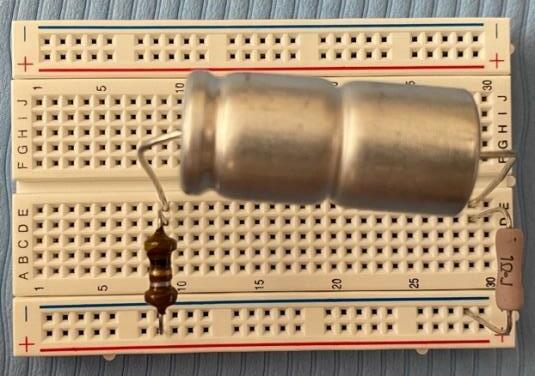
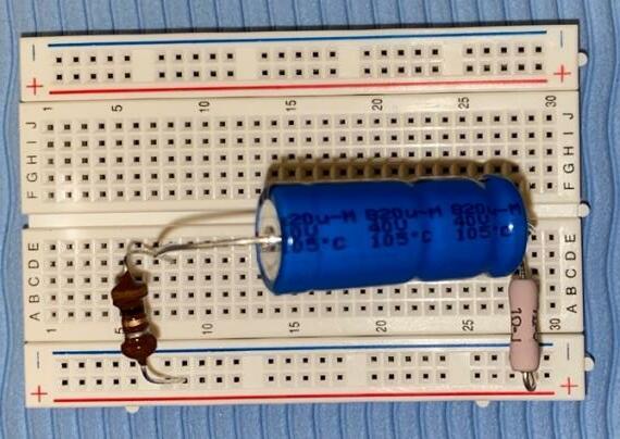
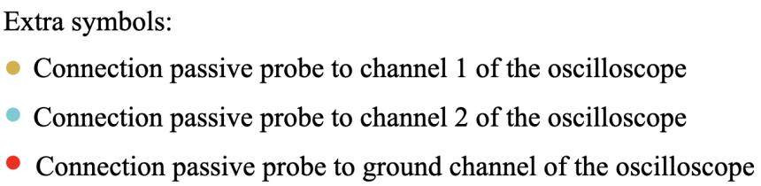
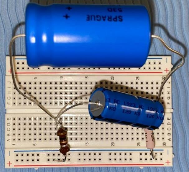
Circuit 2 (Capacitive)

Circuit 3 (Capacitive)

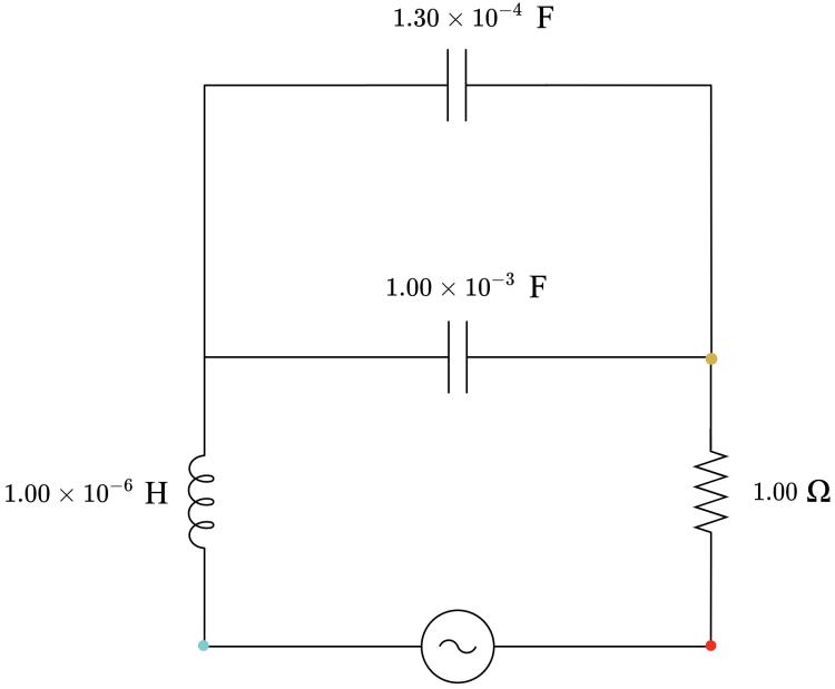
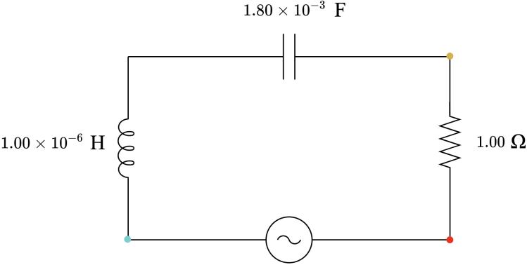
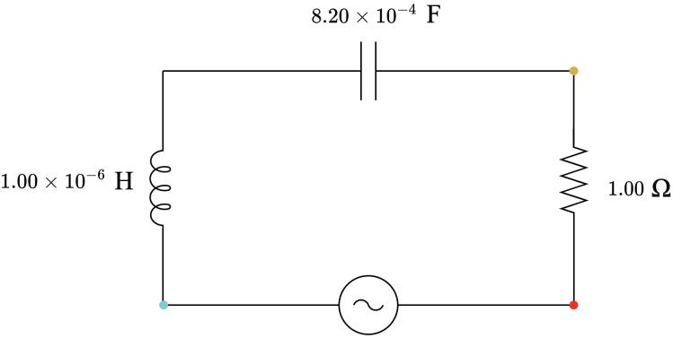
Circuit 5 (Inductive)

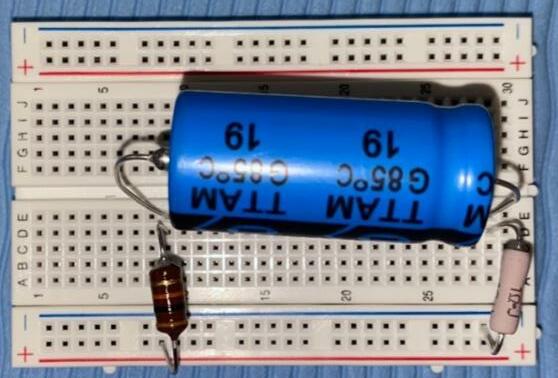
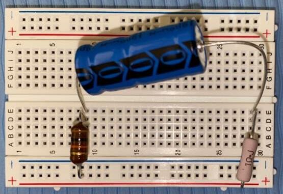
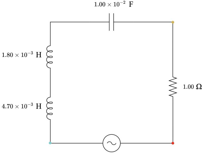
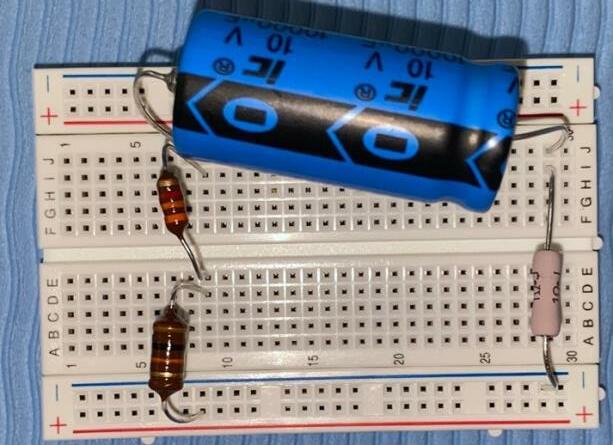
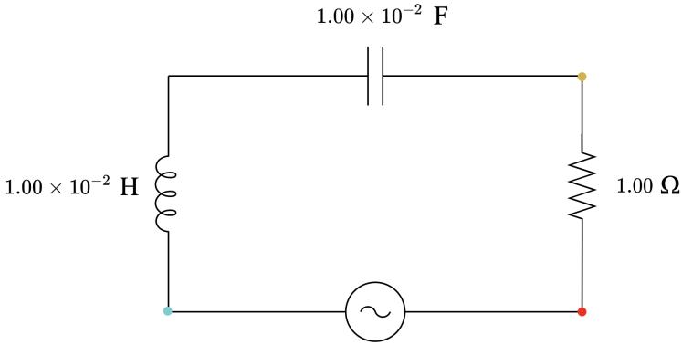
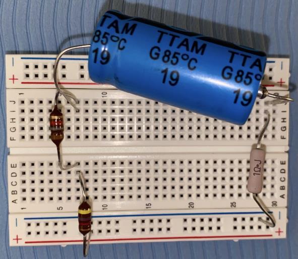
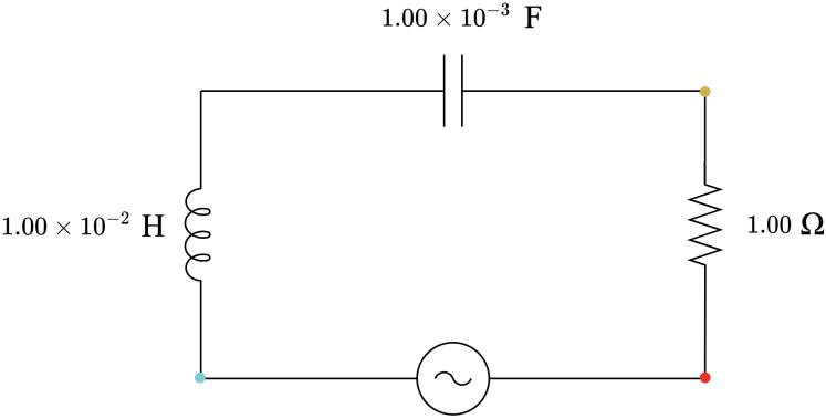
Circuit 6 (Inductive)

Circuit 7 (Inductive)

Comparingtheviscosityoffourdifferentliquids

Aim:Tomeasureandcomparetheviscosityoffourdifferentliquids,namely:honey,corn syrup,goldensyrupandmolasses,andtheeffecttheyhaveonthespeedofamarbledropped intoajaroftheliquid.

Backgroundresearch: AccordingtoPrincetonUniversity,“viscosityisameasureofafluid’sresistancetoflow” (n.d.).Liquidswithhighviscositywill“resistmotion”becausetheirmolecularstructure creates“alotofinternalfriction”(PrincetonUniversity,n.d.).Incontrast,liquidswithlow viscosity“floweasily”becausetheirmolecularstructurecreates“verylittlefrictionwhen...in motion”(PrincetonUniversity,n.d.).AccordingtoEducation.com,whenamarbleisdropped intomultipleliquidsofdifferentviscosities,thevelocityofthemarblewillbeslowestinthe liquidthathasthehighestviscosity(n.d.).Furthermore,theviscosityofaliquidisaffectedby temperature(AZoM,2013).Hightemperaturescandecreaseviscosity,andlowtemperatures canincreaseviscosity(AZoM,2013).ViscosityismeasuredinNewton-secondspermeter squared(Ns/m2)(ScienceBuddies,n.d.b).Thefollowingequationcanbeusedtocalculate theviscosityofaliquidwhenamarbleisdroppedintotheliquid(ScienceBuddies,n.d.b): where:

μistheviscosityoftheliquidinNewton-secondspermetersquared(Ns/m2).

Δρisthedifferenceindensitybetweenthemarbleandtheliquidinkilogramsper metercubed(kg/m3).

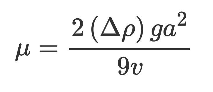
gistheaccelerationduetogravity,9.81meterspersecondsquared(m/s2).

aistheradiusofthemarbleinmeters(m).

vistheaveragevelocity(thedistancethemarblefalls,dividedbythetimeittakesto fall,inmeterspersecond(m/s)).

AccordingtoNASA,thisequationforviscositydependsoncertainassumptions,including: themarblehasreacheditsterminalvelocityandtheReynoldsnumberisverysmall(NASA, 2021).Terminalvelocityreferstothemaximumvelocity(Cain,2010).TheReynoldsnumber referstotheratioofinertialforcestoviscousforces(NASA,2021)anditmustbeverylow, ortheviscositycalculatedusingtheformulaabovewillbeinaccurate(ScienceBuddies, n.d.b).ToensurethattheReynoldsnumberislow,liquidssuchaswateroroilcannotbeused intheformulaabove(ScienceBuddies,n.d.b).

Bothviscosityanddensityarephysicalpropertiesofliquids(Pearson,2017).Bothdensity andviscosityareaffectedbytemperature(Druin,1968).Densityisdefinedasthe“measure ofspacesbetweentwoparticlesinagivenfluid”andreferstohowcompactasubstanceis (BYJU'S,n.d.).Whenaliquidisheated,thespacebetweenitsparticlesincreases,which resultsinadecreaseinfluiddensity(Druin,1968).Duetoreducedfluiddensity,theliquid becomeslessviscous(Druin,1968).Therefore,asthetemperatureofaliquidincreases,its

densitydecreasesandtheliquidbecomeslessviscous(Druin,1968).Herearethedensitiesof somecommonhouseholdliquids:

● Thedensityofhoneyis1360kg/m3 (SoftSchools,n.d.).

● Thedensityofcornsyrupis1380kg/m3 (Elert,n.d.).

● Thedensityofgoldensyrupis1430kg/m3 (Rust,n.d.).

● Thedensityofmolassesis1600kg/m3(Numerade,n.d.). Storingthesecommonhouseholdliquidsbecomeseasierwithknowledgeofviscosityandits relationshipwithtemperature.Thiscanhelponedeterminewhethercertainliquidsshouldbe storedintherefrigeratororatroomtemperature.

Thescientificconceptofviscosityhasimportantreal-lifeapplications.Forexample,knowing theviscosityofaliquidcanbebeneficialwhenpouringliquidintoajar,orspreadingliquid ontoasurface.Therearemanypracticalapplicationsforviscosityineverydaylife.For example,accordingtoQSStudy,viscosityiscrucialininkjetprinting,andfoodanddrink manufacturing(n.d.).Viscosityisalsoimportantinlubricationinvehiclesasitaffects“the rateofoilconsumption”andacar’sabilityto“startinhotorcoldconditions”(QSStudy, n.d.).Additionally,viscosityisalsocrucialinthecookingindustryasit“playsasignificant roleinthepreparationandservingoffood”throughtheuseofcookingoilsandfatsaswellas in“sauces,soups,andstews”(QSStudy,n.d.).Moreover,manufacturingequipmentalso utilisesknowledgeofviscosityaslubricationisveryimportantinthemanufacturingindustry (ThoughtCo,n.d.).Forexample,lubricantsprovideprotectionformovingpartsandcan preventmachinesfrommalfunctioning(ThoughtCo,n.d.).Inaddition,amajorconsideration inthemedicalindustryisbloodviscosity(ThoughtCo,n.d.).Recognisingtheviscosityof bloodiscriticalwhenperforminginjectionsorbloodtransplantsasbloodwithahigh viscosity“canformdangerousinternalclots”andbloodwithalowviscosityisunabletoclot, whichcanleadto“bloodlossandevendeath”(ThoughtCo,n.d.).Itisclearthatviscosityis crucialinmanyareasofeverydaylifeandifviscosityisnotregulatedproperlyinmany industries,itwillhavedevastatingconsequences.

Furthermore,therearereal-lifeexampleswhereknowledgeofviscositycouldsavelives.For example,theGreatMolassesFloodof1919wasatragichistoricaleventwhere21peoplelost theirlives(“GreatMolassesFlood”,2021).ThefloodoccurredinBoston,USA,on15 January1919,whenagiantsteeltankcontainingmolassesexploded(Sohn,2020). Approximately7.5millionlitresofmolassesspreadinasimilarfashiontoatsunamiwave, reachingspeedsofupto56km/h(Lyons,2009).Thiswasadevastatingevent,withover150 peopleinjured(Sohn,2020).Thefloodofmolassesdestroyedbuildings,carsandother importantinfrastructure(“GreatMolassesFlood”,2021).Duetothecoldweatherontheday onwhichthetankexploded,themolassesbecameveryviscousandthisledtoanincreased numberofcasualties(Sohn,2020).Casualtiesresultedfrompeoplebeingpinnedunderfallen infrastructureandbecomingsubmergedintheviscousliquid(Lyons,2009).Accordingto Encyclopaedia Britannica,rescueeffortswouldhavebeeneasieriftheweatherwaswarmer. Itisclearthatviscosityhasmanyeverydayapplicationsandaninterestingbuttragic connectiontohistory.

Hypothesis:Thatthemarblewilltakethelongestamountoftimetoreachthefinishingline whenthejarcontainsmolasses,followedbygoldensyrup,cornsyrupandhoney.Thisis becausemolasseswillhaveahigherviscositythantheotherliquidsasitisverythickwhich willcreateresistance,causingthemarbletofallslowly.Thishypothesisisbasedonthe backgroundinformationthatmolasseshasthehighestdensityofthefourliquids,of1600 kg/m3,whichmeansitisacompactliquid,whichwillcreateresistanceagainstthemarbleand causeittofallslowly.

Variables:

Variable Information

Independent Theviscosityofeachliquid (honey,cornsyrup,golden syrupandmolasses), measuredinNewton-seconds permetersquared(Ns/m2).

Dependent Theamountoftimeittakes forthemarbletoreachthe finishingline,measuredin seconds.

Controlled Variables

Temperatureoftheliquid

Howthevariablewascontrolled

N/A

N/A

Volumeoftheliquid

Sizeofmarble

Massofmarble

Typeofjar

Heightatwhichthemarbleis dropped

Equipmentandmaterials:

Thetemperatureofeachliquidwas measuredbeforeeachtrial,toensure theliquidswerethesametemperature foreachtrial.

Thevolumeoftheliquid(350mL)was measuredusingameasuringjug.

Thesamesizedmarblewasusedinall liquidsandtrials.

Themassofeachmarblewasthesame (5g).

Fouridenticaltransparentglassjarsof height17cmanddiameter6cmwere used.

Theheightatwhicheachmarblewas droppedwasthesame(17cm).

❖ 4identicaltransparentglassjarsofheight17cmanddiameter6cm

❖ 4identicalmarblesofdiameter1.5cmandmass5g

❖ 1measuringjugofcapacity500mL

❖ 4tablespoons

❖ 1stopwatch

❖ 1blackmarkerpen

❖ 1ruler(30cm)

❖ 1thermometer

❖ 1labcoat

❖ 1pairofsafetyglasses

❖ 1teatowel(30cmby40cm)

❖ 350mLhoney

❖ 350mLcornsyrup

❖ 350mLgoldensyrup

❖ 350mLmolasses

Pleasenotethatthisexperimentalsorequiresatableoraflatsurface,andaccesstoasink withrunningwater.

RiskAssessment: Risk Precaution

Brokenglass-Iftheglassjarsorthe marblesbreak,brokenglassmaycutany exposedskin.

Topreventtheglassjarsandmarblesfrom breaking,handlethemcarefully.Alabcoat willalsoreducetheamountofskinexposed andthereforereduceone’schanceof becominginjured.Safetyglassesmustalso beworntoprotecttheface.

Ifglassdoesbreak,ensureitisimmediately andthoroughlysweptupusingadustpan andbroom.

Substancespills-Ifthehoney,cornsyrup, goldensyrupormolassesspillonthefloor, theywillbecomeasafetyhazardandmay causeinjury.

Topreventhoney,cornsyrup,goldensyrup ormolassesfromspilling,handlethe substancescarefullyandinspectalljarsand containersforleaks,cracksorevidenceof deteriorationbeforeconductingthe experiment.Alabcoatandsafetyglasses mustbewornduringtheexperimentto preventthesubstancesfromirritatingthe eyesandskin.

Method:

1.Fourjarswerecarefullyplacedonthetable.

2.350mLofhoneywasmeasuredusingthemeasuringjug,andpouredintothefirstjar.

3.Themeasuringjugwaswashedthoroughlyanddried.

4.350mLofcornsyrupwasmeasuredusingthemeasuringjug,andpouredintothe secondjar.

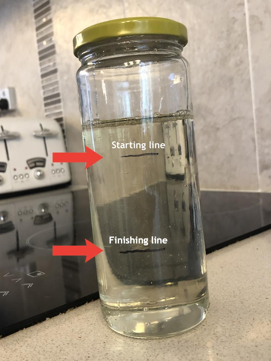
5.Themeasuringjugwaswashedthoroughlyanddried.

6.350mLofgoldensyrupwasmeasuredusingthemeasuringjug,andpouredintothe thirdjar.

7.Themeasuringjugwaswashedthoroughlyanddried.

8.350mLofmolasseswasmeasuredusingthemeasuringjug,andpouredintothefourth jar.

9.Oneachjar,astartinglinewasdrawn2cmbelowthetopofthesurfaceoftheliquid usingamarkerpen(asshowninFigure1).

10.Oneachjar,afinishinglinewasdrawn5cmabovethebottomofthejarusinga markerpen(asshowninFigure1).

Figure1

11.Thedistancebetweenthestartinglineandfinishinglinewasmeasuredandrecorded foreachjartoensuretheywerethesamedistanceapart,andthefollowingtablewas drawn(Table1):

Table1

Distancebetweenstartingandfinishingline (cmto2d.p.)

Liquid

Honey Cornsyrup Goldensyrup Molasses

12.Theequipmentsetupwascheckedtoensurethatitmatchedthefollowingdiagram, Figure2.

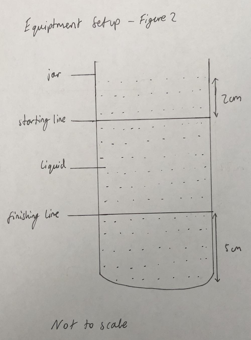
13.Thefollowingtable(Table2)wasdrawn.

Table2

Timetakenforthemarbletotravelfromthestartinglinetothe finishingline(secondsto2d.p.)

Trial1 Trial2 Trial3 Trial4 Trial5 Average

Liquid

Honey Cornsyrup Golden syrup Molasses

14.Thefollowingtable(Table3)wasdrawn.

Table3

Temperatureoftheliquidbeforeeachtrial(℃ tothenearest degree)

Trial1 Trial2 Trial3 Trial4 Trial5 Average

Liquid

Honey Cornsyrup Golden syrup

Molasses

15.Thefollowingtable(Table4)wasdrawn.

Table4

Qualitativeobservationsmadeduringtheexperimentalprocedure Honey

Trial Observations

Observations

Cornsyrup

Observations

syrup

16.Thetemperatureoftheliquidinthefirstjarwasmeasuredusingathermometerand recordedinTable3.

17.Thethermometerwaswashedthoroughlyanddried.

18.Amarblewasdroppedintothemiddleofthefirstjarfromaheightequaltotherimof thejar.

19.Ateye-level,whenthemarblereachedthestartingline,thestopwatchwasstarted.

20.Whenthemarblereachedthefinishingline,thestopwatchwasstopped.

21.ThetimeonthestopwatchwasrecordedinTable2andthestopwatchwasreset.

22.QualitativeobservationswererecordedinTable4.

23.Usingatablespoon,themarblewasretrievedfromthejarandthoroughlywashedand dried.

24.Steps16-23wererepeated4moretimes.

25.Steps16-24wererepeatedfortheotherthreejars.

26.Theaveragetimetakenforthemarbletotravelfromthestartinglinetothefinishing linewascalculatedandrecordedinTable2.

27.TheaveragetemperatureoftheliquidwascalculatedandrecordedinTable3.

Results:

Theresultsoftheexperimentareshowninthetablesandgraphsbelow

Table1

Distancebetweenstartingandfinishingline (cmto2d.p.)

Honey 5.50

Liquid

Cornsyrup 5.50 Goldensyrup 5.50 Molasses 5.50

Table2

Timetakenforthemarbletotravelfromthestartinglinetothe finishingline(secondsto2d.p.)

Trial1 Trial2 Trial3 Trial4 Trial5 Average

Liquid

Honey 15.56 15.13 16.17 16.39 16.05 15.86 Cornsyrup 104.80 101.42 100.04 103.50 99.51 101.85 Golden syrup 16.95 16.89 16.98 16.90 16.22 16.79 Molasses 2.92 2.15 3.05 2.02 1.92 2.41

Table3

Temperatureoftheliquidbeforeeachtrial(℃ tothenearest degree)

Trial1 Trial2 Trial3 Trial4 Trial5 Average

Honey

Liquid

Cornsyrup 20 20 20 20 20 20 Golden syrup 20 20 20 20 20 20 Molasses 20 20 20 20 20 20

Qualitativeobservationsmadeduringtheexperimentalprocedure Honey

Trial Observations

Pre-trial

Thehoneyhadastrongsmellandwassticky.Theliquidwasbrownin colourandtransparent.

1 Whenthemarblewasdroppedinthehoney,themarblemovedrather quicklyatfirst,thensettledintoasteady,slowspeedbythetimeitpassed thestartingline.Themarblethencontinuedtofallslowly.

2 Asthemarbleenteredthehoney,alargeholeappearedwherethemarble wasandthehoneysankwiththemarble.Whenthemarblewasfully submerged,theholedisappearedandthehoneybecamelevelagain.The marblefellveryslowly.

3 ThistrialseemedslightlyslowerthanTrial1andTrial2.Themarblefellat averyslowrateandsmallbubblesbegantoappearintheliquid.

4 Themarbleseemedtofallveryslowlythroughthehoneyandmoresmall bubblesappeared.

5 Themarbleslowlysankthroughthehoneyandseveralsmallbubbleswere visible.

Cornsyrup

Trial Observations

Pre-trial

Thecornsyrupwasconsiderablythickerthanthehoneyandalsorather sticky.Therewasnoapparentscent.Thecornsyrupitselfwastransparent andcolourless.

1

Whenthemarblewasdroppedintothecornsyrup,therewasalmostno movementatallandthemarblefellextremelyslowly.

2 Themarbleslowlysankthroughthecornsyrupandsmallbubblesbecame visible.Themarbleseemedtofallslightlyfasterthantheprevioustrial.

3 Themarblefellveryslowlythroughthecornsyrupandevenmorebubbles appearedinthethickliquid.

4 Themarblefellextremelyslowlythroughtheliquidandsomemorebubbles appearedinthecornsyrup.

5

Inthistrial,themarblecontinuedtomoveveryslowlythroughthecorn syrup,butitseemedtobeslightlyfasterthantheprevioustrials.Lotsof smallbubbleswerevisibleduringthistrial.

Goldensyrup

Trial Observations

Pre-trial

1

Thegoldensyrupwasthick,yellowy-brownincolourandasweetodour waspresent.

Whenthemarblewasdroppedintheliquid,itfellquicklyatfirst,then settledintoasteady,slowpacebeforeitpassedthestartingline.Themarble continueditsslowdescentpastthefinishingline.

2 Themarblefellthroughtheliquidinasimilarfashiontotheprevioustrial. Nobubbleswerevisible.

3

Asthemarbleslowlyfellthroughtheliquid,smallbubblesappeared.

4 Themarbleslowlysankthroughthegoldensyrupandsmallbubbles becamevisible.Themarbleseemedtofallslightlyfasterthaninthe previoustrial.

5 Morebubblesappearedinthistrialwhenthemarblefellthroughthegolden syrup.Thistrialseemedtobefasterthanalloftheprevioustrials.

Molasses

Trial Observations

Pre-trial

1

Themolasseswasadark,barelytransparentliquidthathadastrongodour. Itwasratherthinandsticky.

Thedarkcolourofthemolassesmadeitslightlydifficulttoseethemarble. Luckilythemarblewasbrightlycolouredsoitwasvisibleasitfellthrough theliquid.Themarbleseemedtofallveryquickly.

2

Inthistrial,themarbleseemedtofallveryquicklythroughthemolasses andnovisiblebubblesoccurredinthemolassesliquiditself.

3 Themarbleappearedtofallveryfastthroughthemolasses.Again,no bubbleswerevisible.

4 Whenthemarblewasdroppedintothemolasses,itappearedtofallvery quickly.Nobubbleswerevisible.

5

Inthistrial,themarbleappearedtofallfasterthaninalloftheprevious trials.Themarblecontinuedtomoveveryquicklythroughthemolasses.

Qualitativeobservations-photographs

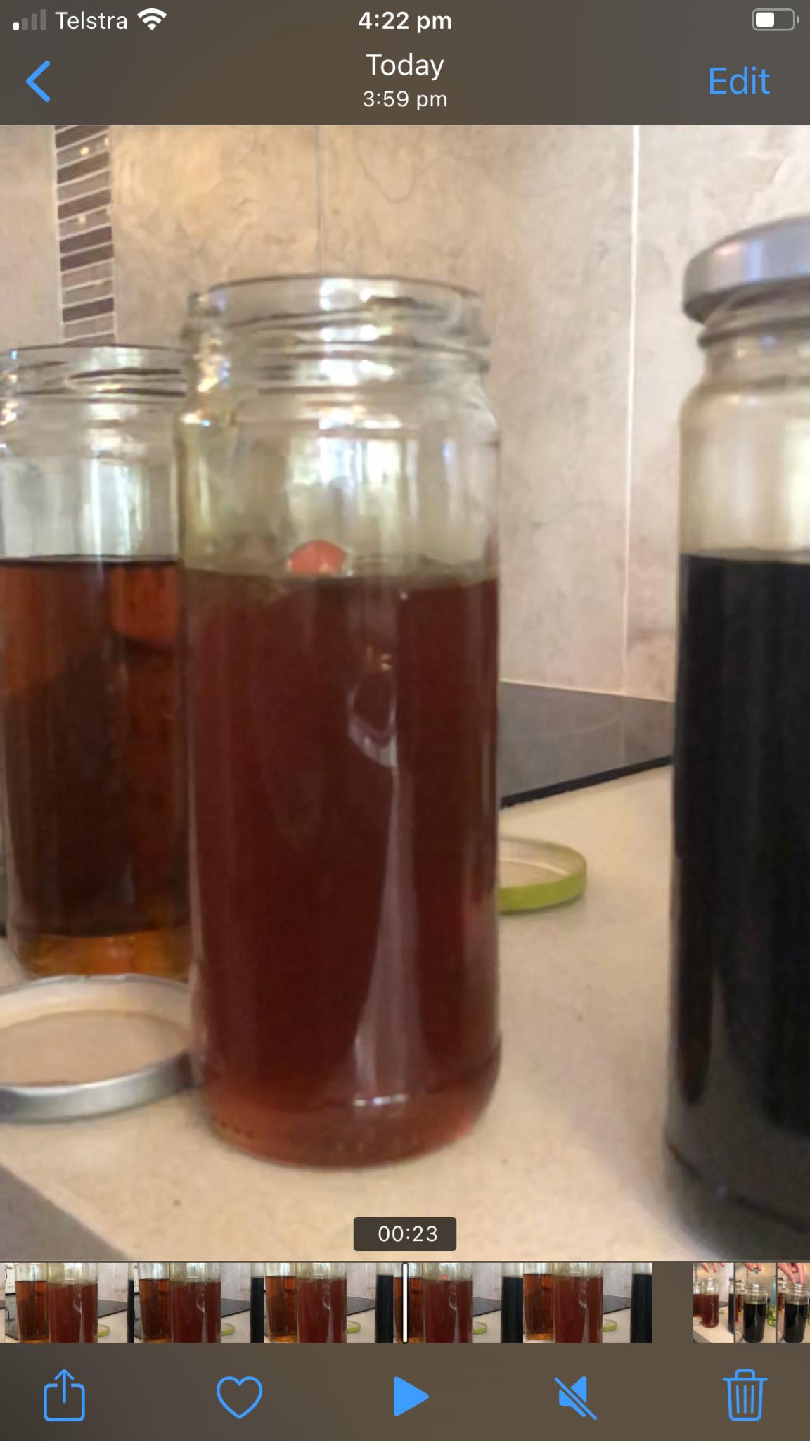
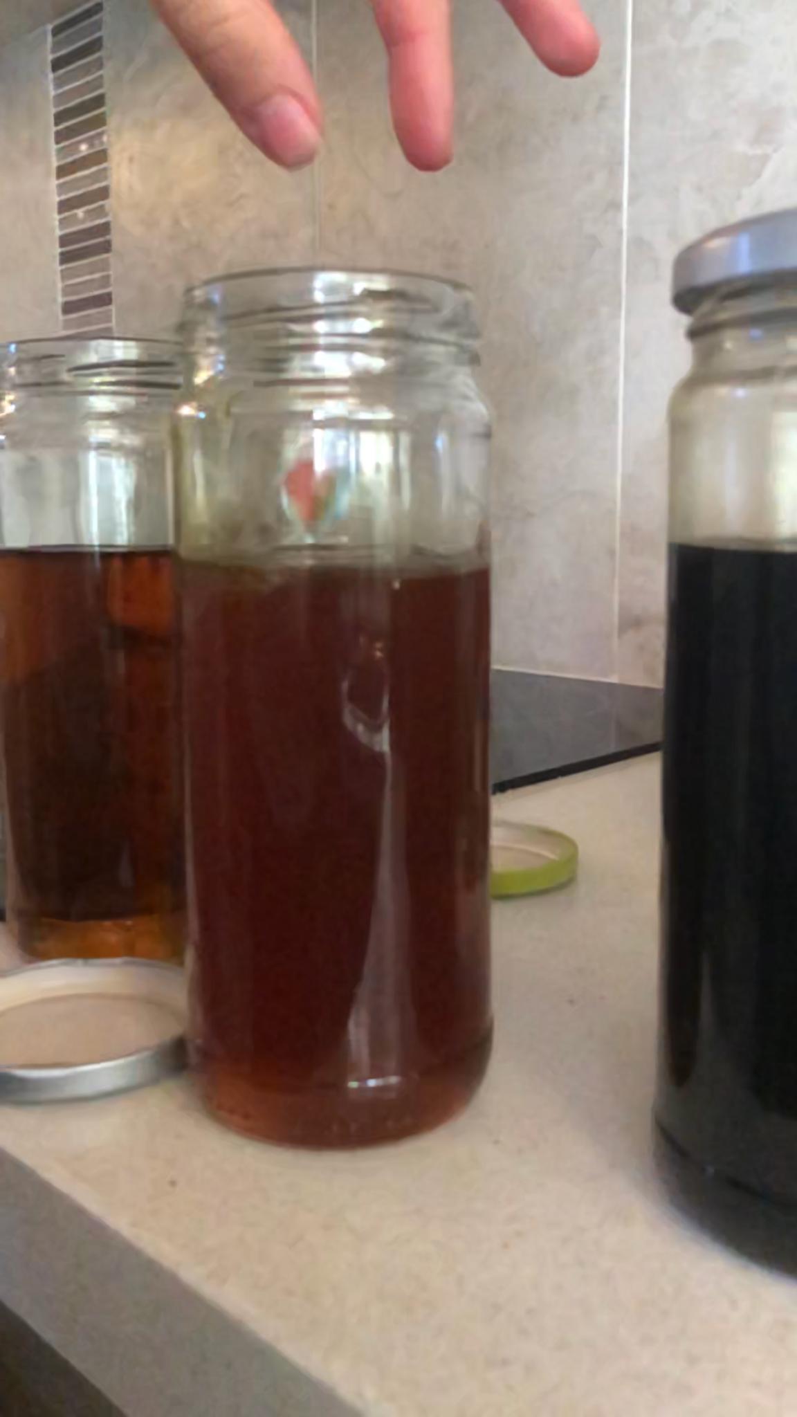
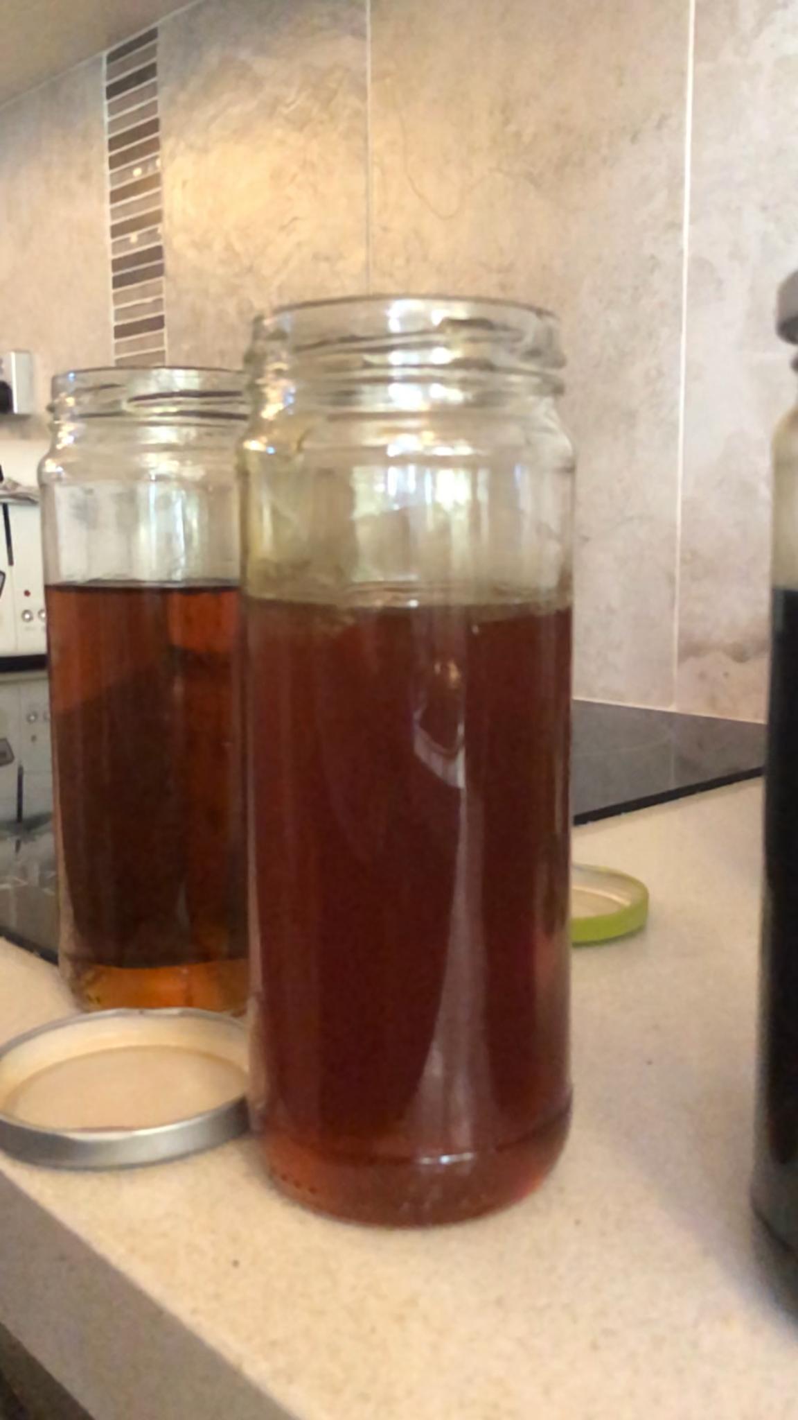
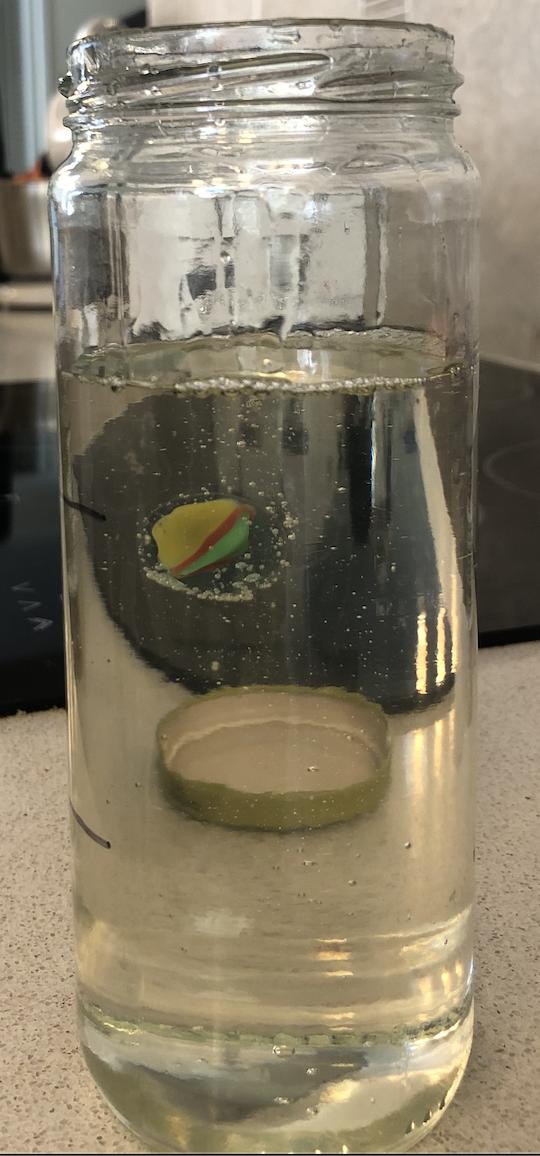
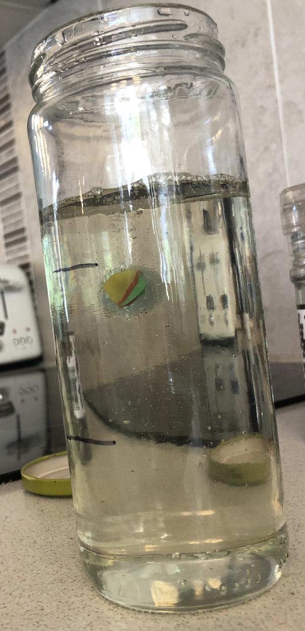
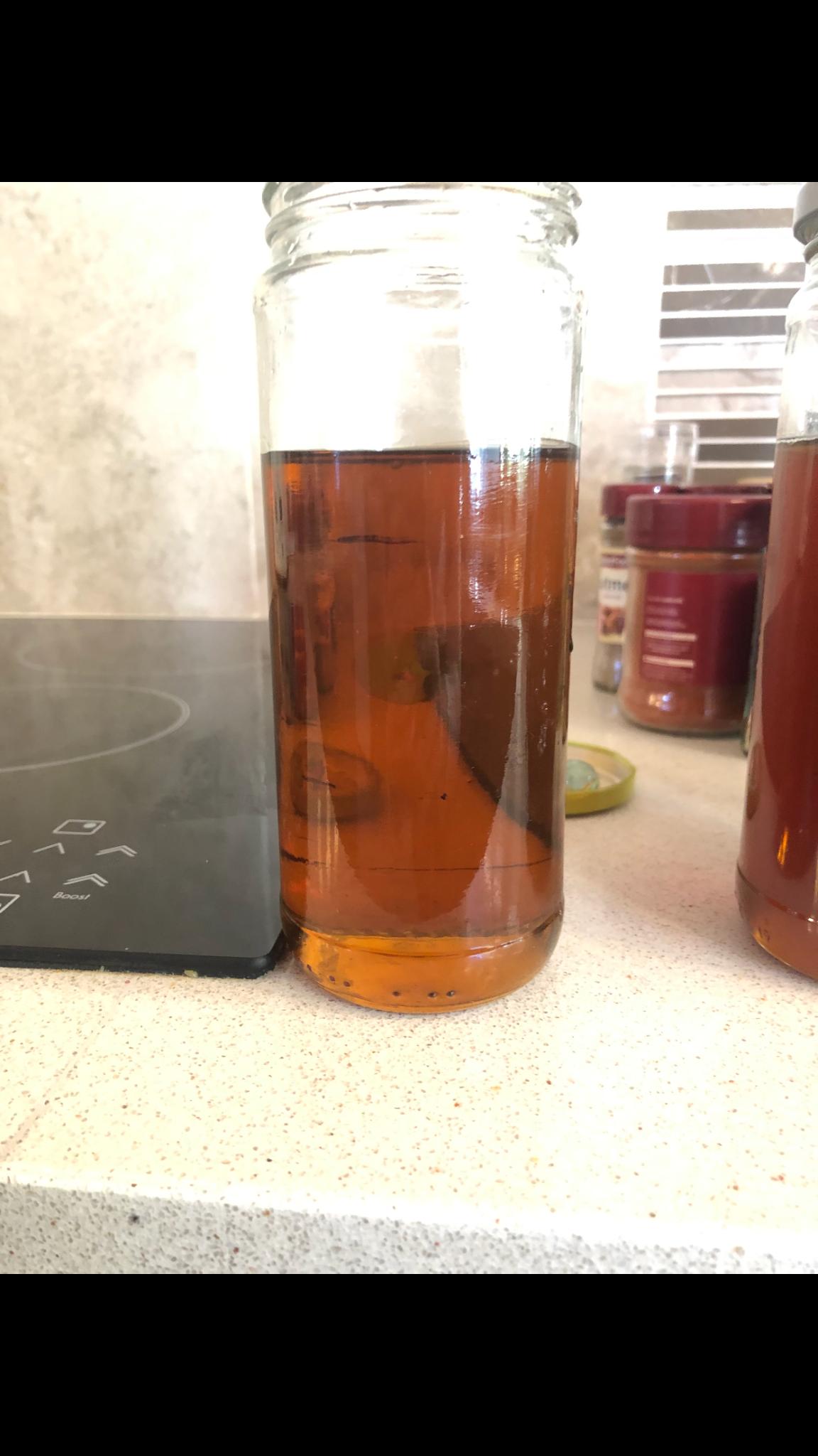
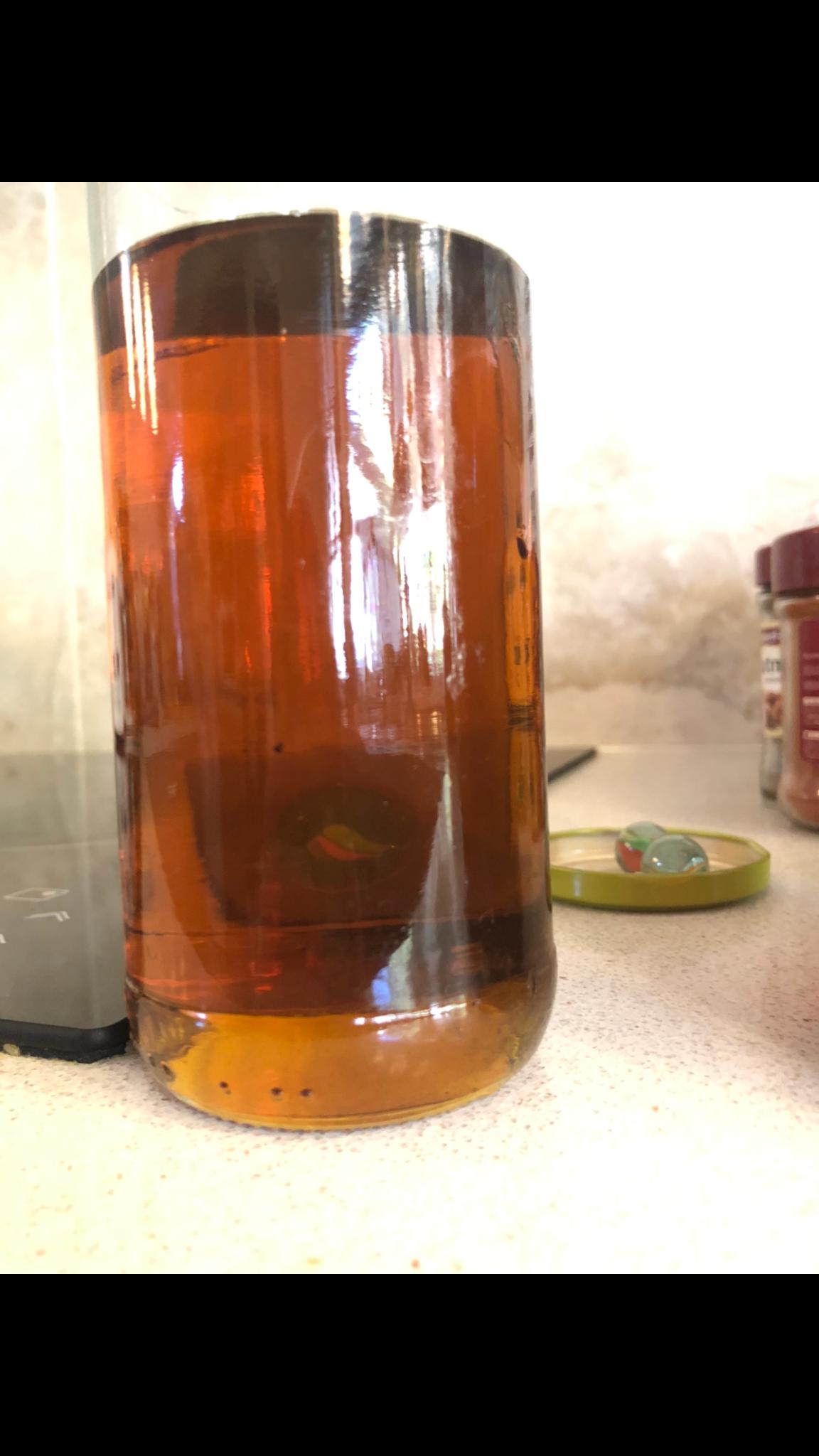
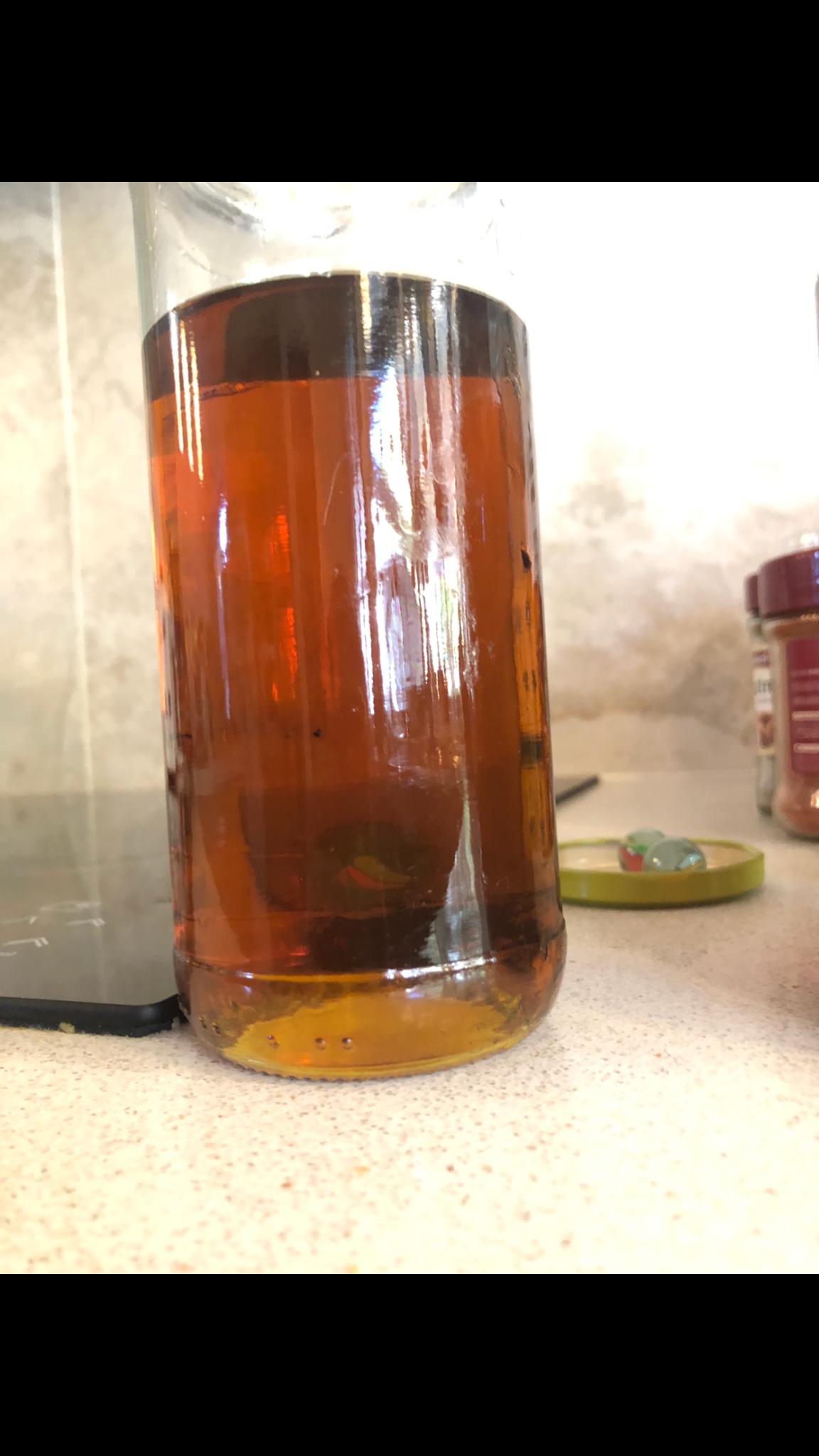
Processeddata:

Table5

Theaverageandthestandarddeviationoftheresultsofthetimetakenfor themarbletotravelfromthestartinglinetothefinishingline(to2d.p.)

Average (s) Standarddeviation

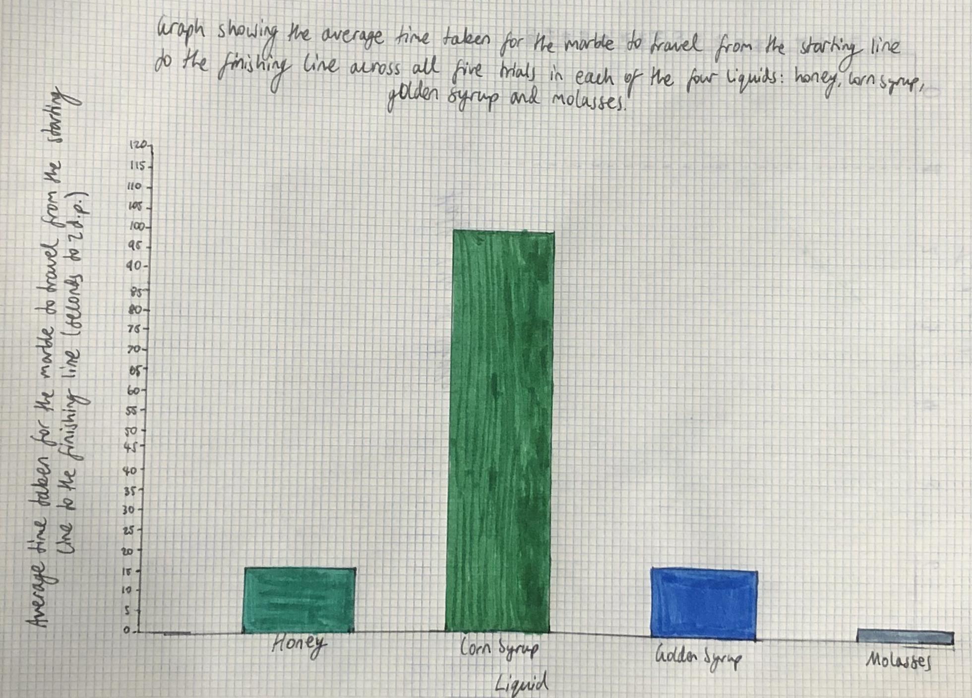
Honey 15.86 0.51

Liquid

Cornsyrup 101.85 2.26 Goldensyrup 16.79 0.32 Molasses 2.41 0.53

ThestandarddeviationvalueswerecalculatedusingtheSTDEVfunctioninMicrosoftExcel. Thisfunctionhasthefollowingformula:

Standarddeviation= whereisthesamplemeanand n isthesamplesize. Figure3

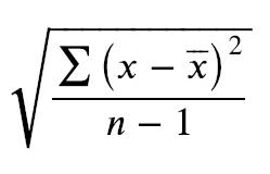
Figure5

Calculatingviscosity:

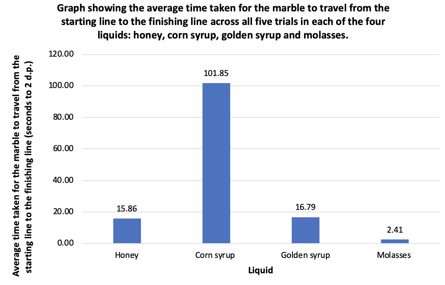
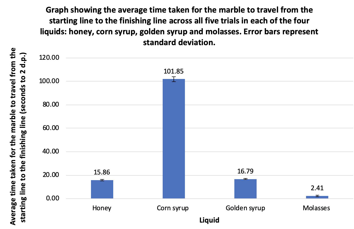
Thefollowingequationwasusedtocalculatetheviscosityofeachliquid:

where:

μistheviscosityoftheliquidinNewton-secondspermetersquared(Ns/m2). Δρisthedifferenceindensitybetweenthemarbleandtheliquidinkilogramspermeter cubed(kg/m3).

gistheaccelerationduetogravity,9.81meterspersecondsquared(m/s2). aistheradiusofthemarbleinmeters(m). vistheaveragevelocity(thedistancethemarblefalls,dividedbythetimeittakestofall,in meterspersecond(m/s)).

Calculatingthedensityofthemarble

1.Massofmarbleis5gwhichequals0.005kg

2.Diameterofthemarbleis1.5cmsotheradiusishalfthediameter,whichequals0.75cmor 0.0075m

3.Volumeofsphere=4/3πr3

Therefore,V=4/3xπx0.00753 V=0.00000176714m3

4.Density=mass/volume Therefore,densityofthemarble=0.005kg/0.00000176714m3 Density=2829.421211kg/m3

Densityofeachliquid(sourcedfrombackgroundresearch)

Thedensityofhoneyis1360kg/m3

Thedensityofcornsyrupis1380kg/m3

Thedensityofgoldensyrupis1430kg/m3 Thedensityofmolassesis1600kg/m3

Calculatingaveragevelocityofthemarble

Theaveragetimetakenforthemarbletotravelfromthestartinglinetothefinishingline(a distanceof5.5cm)wasusedtocalculatetheaveragevelocityofthemarbleineachliquid,as follows:

Velocityofthemarbleinhoney

Velocity=distance/time

V=0.055m/15.86s

V=0.055/15.86m/s

Velocityofthemarbleincornsyrup

Velocity=distance/time

V=0.055m/101.85s

V=0.055/101.85m/s

Velocityofthemarbleingoldensyrup

Velocity=distance/time

V=0.055m/16.79s

V=0.055/16.79m/s

Velocityofthemarbleinmolasses

Velocity=distance/time

V=0.055m/2.41s

V=0.055/2.41m/s

Calculatingtheviscosityofeachliquid

Theviscosityofeachliquidwascalculatedbysubstitutingtheappropriatevaluesintothe equation

Honey

Viscosity=(2x(marbledensity-honeydensity)xgxa^2)/(9x(0.055/time))

Viscosity=(2x(2829.421211-1360)x9.81x0.0075^2)/(9x(0.055/15.86))

Viscosity=51.95960232

Viscosity=51.96Ns/m2

Cornsyrup

Viscosity=(2x(marbledensity-cornsyrupdensity)xgxa^2)/(9x(0.055/time))

Viscosity=(2x(2829.421211-1380)x9.81x0.0075^2)/(9x(0.055/101.85))

Viscosity=329.1334156

Viscosity=329.13Ns/m2

Goldensyrup

Viscosity=(2x(marbledensity-goldensyrupdensity)xgxa^2)/(9x(0.055/time))

Viscosity=(2x(2829.421211-1430)x9.81x0.0075^2)/(9x(0.055/16.79))

Viscosity=57.62463193

Viscosity=57.62Ns/m2

Molasses

Viscosity=(2x(marbledensity-molassesdensity)xgxa^2)/(9x(0.055/time))

Viscosity=(2x(2829.421211-1600)x9.81x0.0075^2)/(9x(0.055/2.41))

Viscosity=7.266524803

Viscosity=7.27Ns/m2

Therefore,theviscosityofeachliquidindescendingorder,roundedto2decimalplaces,is: cornsyrup(329.13Ns/m2),goldensyrup(57.62Ns/m2),honey(51.96Ns/m2)andmolasses (7.27Ns/m2).

Discussion:

Table2showsthetimetakenforthemarbletotravelfromthestartinglinetothefinishing lineduringthefivetrialsineachliquid.Thedatarevealsthattheaveragetimetakenforthe marbletoreachthefinishinglineineachliquidwasasfollows(indescendingorder):101.85s forcornsyrup,16.79sforgoldensyrup,15.86sforhoneyand2.41sformolasses.Table5and Figure5containthestandarddeviationoftheseresults.Thestandarddeviationindicatesthe spreadofthedata.Thedatafromthecornsyruptrialshadthehigheststandarddeviation, 2.26.Thiswasfollowedbythestandarddeviationformolasses,0.53,andthestandard deviationforhoney,0.51.Lastly,thesmalleststandarddeviationwasforgoldensyrup,0.32. Asthestandarddeviationforeachliquidwassmall,thisrevealsthattherewaslittlevariation inthedatacollectedandthedataisthereforemorelikelytobereliable.

Table1confirmsthatthedistancebetweenthestartinglineandfinishinglinewasconsistent overalljars,andwas5.50cm.Table3confirmsthatthetemperatureoftheliquidbeforeeach trialineachliquidwasconsistent,at20℃.Theseweretwoimportantcontrolledvariables whichincreasedthevalidityoftheexperiment.Thebackgroundresearchemphasisedthe importanceofcontrollingtemperatureaswhenthetemperatureofaliquidincreases,its densitydecreasesandtheliquidbecomeslessviscous(Druin,1968).

SeveraltrendsarosefromFigure3andFigure4,ascanbeseenfromtheheightofthe columnsinthesecolumngraphs.Forexample,itisevidentthatthemarbletookthelongest amountoftimetotravelfromthestartinglinetothefinishinglineonaverageincornsyrup, byasignificantmargin,asitisbyfarthetallestcolumninthegraphs.Additionally,the averageresultsforhoneyandgoldensyrupweresimilar,beingonly0.93sapart,asshownby thecolumnsofsimilarheight.Finally,anothertrendisthatthemarbletooktheshortest amountoftimetotravelfromthestartinglinetothefinishinglineonaverageinmolasses,as indicatedbytheshortestcolumn.

Thefollowingequationfromthebackgroundresearch(ScienceBuddies,n.d.b)wasusedto calculatetheviscosityofeachliquid:

Substitutingtherelevantinformationintotheequationrevealedthattheviscosityofeach liquidindescendingorderis:cornsyrup(329.13Ns/m2),goldensyrup(57.62Ns/m2),honey (51.96Ns/m2)andmolasses(7.27Ns/m2).Thisorderreflectsthatoftheaveragetimetaken forthemarbletoreachthefinishinglineineachliquid.Thisalsoissupportedbythe backgroundresearch,whichstatesthatwhenamarbleisdroppedintomultipleliquidsof

differentviscosities,thevelocityofthemarblewillbeslowestintheliquidthathasthe highestviscosity(Education.com,n.d.).

Evaluation:

Theresultsfromthisexperimentarereliablebecauseeachtrialwasrepeated5timesandthe datacollectedwasincloserangeoftheothervalues,whichsuggestsconsistencyand reliability.ThisisfurthersupportedbythelowstandarddeviationscalculatedinTable5.The experimentconductedwasvalidbecauseallthevariablesapartfromtheindependentand dependentvariableswerecontrolled.Furthermore,allmeasurementswereprecise,using equipmentsuchasmeasuringjugsandthermometers,andtherecordeddataisthereforevalid. Thedatawasalsoaccuratelydisplayedandaconclusion,fulfillingtheaimoftheexperiment, couldbeformedbasedonthedata.Themethodultimatelyallowedappropriatedatatobe collectedtoeithersupportorrefutethehypothesis.

However,threemainsourcesoferrorwereidentifiedinthisexperiment:

1.Whenthemarblewasremoved,someliquidwasalsoremovedalongsidethemarble. Thiscausedlessthan350mLtoberemainingwithinthejaraftereachtrialandmay haveimpactedthetimeatwhichterminalvelocitywasachievedbythemarble, overallimpactingthedatacollected.

2.Thisexperimentreliesonthereactiontimeofthepersontimingthemarble’sdescent fromthestartinglinetothefinishingtime.Reactiontimeisnotveryreliablebecause therearemanyfactorsthatcanimpactit,suchasamountofsleep,ageandcaffeine intake(Taheri&Arabameri,2012).Theaveragehumanreactiontimeis approximately250milliseconds(Ackerman,2019).Thismakesthedatacollectedless accurate.

3.Duringthethirdorfourthtrialforallliquidsexceptmolasses,smallbubblesstartedto appear.Thesewerelikelyairbubblescausedbythemarblemovingthroughtheliquid. Theseairbubblesimpactedtheconsistencyoftheliquid,whichmayhaveaffectedthe overallresultsoftheexperiment.

Toaddressthesethreesourcesoferror,thefollowingmodificationscouldbemade:

1.Beforeconductingtheexperiment,the350mLlinecouldbemarkedonthejar.This wouldenablethejarstobesupplementedwithadditionalliquid,ifrequired,toensure 350mLisinthejarbeforeeachtrial.

2.Toeliminatetheexperiment’srelianceonhumanreactiontime,eachtrialcouldbe filmedandthevideotimestampswouldbeusedtodeterminetheamountoftimetaken forthemarbletofallfromthestartinglinetothefinishingline.

3.Aftereachtrial,theliquidmustbelefttosettle,waitinguntilnobubblesarevisible, beforeconductingthenexttrial.Thiswillpreventbubblesfromimpactingthetrial’s results.

Conclusion:

Inthisexperiment,thehypothesiswasrefuted.Thehypothesisstatedthatthemarblewilltake thelongestamountoftimetoreachthefinishinglinewhenthejarcontainsmolasses,

followedbygoldensyrup,cornsyrupandhoney.However,theexperimentalresultsindicated thatthemarbletookthelongestamountoftimetoreachthefinishinglineincornsyrup (101.85s),followedbygoldensyrup(16.79s),honey(15.86s)andmolasses(2.41s),which didnotsupportthehypothesis.Furthermore,thisexperimentconcludedthattheviscosityof eachliquidindescendingorderis:cornsyrup(329.13Ns/m2),goldensyrup(57.62Ns/m2), honey(51.96Ns/m2)andmolasses(7.27Ns/m2).Theaimoftheexperimentwasfulfilledas theviscosityofthefourliquidswasmeasuredandcompared.

Ackerman,E.(2019). Upgrade to Superhuman ReflexesWithout Feeling Like a Robot https://spectrum.ieee.org/enabling-superhuman-reflexes-without-feeling-like-a-robot

Ahmad,B.(2019). Measuring Viscosity of DifferentFluids Using Ball Drop Method. https://www.researchgate.net/publication/337707277_MEASURING_VISCOSITY_OF _DIFFERENT_FLUIDS_USING_BALL_DROP_METHOD

Ali,H.S.,Al-Zuky,A.A.,Al-Saleh,A.H.,&Mohamad,J.H.(2019).Measureliquidviscosity bytrackingfallingballautomaticallydependingonimageprocessingalgorithm. Journal of Physics: Conference Series. 1294(2),1-15. https://doi.org/10.1088/1742-6596/1294/2/022002

AZoM.(2013). How does Temperature Change Viscosityin Liquids and Gases? https://www.azom.com/article.aspx?ArticleID=10036

Cain,F.(2010). What Is Terminal Velocity? https://www.universetoday.com/73617/terminal-velocity/

CoolScienceExperimentsHeadquarters.(2016,May3). How to test the Viscosity of a Liquid [Video].YouTube.https://www.youtube.com/watch?v=2Gdxu4XcsbY&t=116s

CoolScienceExperimentsHeadquarters.(2020). Viscosityof Liquids Science Experiment. https://coolscienceexperimentshq.com/viscosity-of-a-liquid-experiment/#Video

Druin,M.L.(1968). Viscosity-density correlationof Newtonian liquids [PDF]. https://digitalcommons.njit.edu/cgi/viewcontent.cgi?article=2388&context=dissertation s

Education.com.(n.d.). Marble Race: Finding Viscosityof Fluids. https://www.education.com/science-fair/article/compare-viscosity-fluids/

Elert,G.(n.d.). Density - The Physics Hypertextbook.https://physics.info/density/

GreatMolassesFlood.(2021).In Encyclopaedia Britannica https://www.britannica.com/topic/Great-Molasses-Flood

Ito,M.A.(2012). Marble Viscosity Race [PDF]. https://csef.usc.edu/History/2012/Projects/J0113.pdf

Lyons,C.(2009). A Sticky Tragedy: The Boston MolassesDisaster https://www.historytoday.com/archive/sticky-tragedy-boston-molasses-disaster

Mueller,P.(2018). Let It Flow: How to Calculate Viscosity. https://www.powerblanket.com/blog/let-it-flow/

NationalAeronauticsandSpaceAdministration(NASA).(2021). Reynold’s Number. https://www.grc.nasa.gov/www/BGH/reynolds.html

Numerade.(n.d.). The Density of Molasses. https://www.numerade.com/questions/the-density-of-molasses-is-1600-mathrmkg-math rmm3-find-the-mass-of-the-molasses-in-a-075-l-jar-2/

Pearson.(2017).FluidMechanicsforChemicalEngineers. https://www.informit.com/articles/article.aspx?p=2832417&seqNum=4

PrincetonUniversity.(n.d.). Definition of Viscosity. https://www.princeton.edu/~gasdyn/Research/T-C_Research_Folder/Viscosity_def.html

QSStudy.(n.d.). Practical Applications of Viscosity. https://qsstudy.com/physics/practical-applications-of-viscosity

Robb,A.(2016). Viscosity Experiment. https://study.com/academy/lesson/viscosity-experiment.html

Rust,A.(n.d.). Syrup.https://sites.google.com/site/volcanologyanalogues/home/syrup

Schellart,W.P.(2011).Rheologyanddensityofglucosesyrupandhoney:Determiningtheir suitabilityforusageinanalogueandfluiddynamicmodelsofgeologicalprocesses. Journal of Structural Geology, 33(6),1079-1088. https://doi.org/10.1016/j.jsg.2011.03.013.

ScienceBuddies.(2015,August27).MarbleRace--inLiquid! Scientific American. https://www.scientificamerican.com/article/marble-race-in-liquid/

ScienceBuddies.(n.d.a). Race Your Marbles to Discovera Liquid's Viscosity - Procedure. https://www.sciencebuddies.org/science-fair-projects/project-ideas/Chem_p055/chemist ry/race-your-marbles-to-discover-liquids-viscosity#procedure

ScienceBuddies.(n.d.b). Race Your Marbles to Discovera Liquid's Viscosity - Background. https://www.sciencebuddies.org/science-fair-projects/project-ideas/Chem_p055/chemist ry/race-your-marbles-to-discover-liquids-viscosity#background

SoftSchools.(n.d.).Reynold'sNumberFormula. https://www.softschools.com/formulas/physics/reynolds_number_formula/78/

Sohn,E.(2020).WhytheGreatMolassesFloodWasSoDeadly. https://www.history.com/news/great-/molasses-flood-science

Taheri,M.,&Arabameri,E.(2012).Theeffectofsleepdeprivationonchoicereactiontime andanaerobicpowerofcollegestudentathletes. AsianJournal of Sports Medicine, 3(1),15–20.https://doi.org/10.5812/asjsm.34719

Tang,X.J.(2016).Measurementsoffluidviscosityusingaminiatureballdropdevice. AIP Publishing.87(5),054301.https://doi.org/10.1063/1.4948314

ThoughtCo.(n.d.). What Is Viscosity in Physics? https://www.thoughtco.com/viscosity-2699336

Warnant,P.,Arena,P.,Burrows,K.,Lofts,G.,Evergreen,M.J.(2017). Jacaranda Core Science Stage 5 NSW Australian curriculum.(2nded.).Milton:JohnWiley&Sons Australia.

SRP - The effect of sugar concentration on fermentation Sophie Rigon

Aim: Toinvestigatetheeffectofincreasedsugarconcentrationontherateoffermentationwithyeastby measuringthepercentageofalcoholproducedbythefermentationofliquidscontainingdiffering concentrations of sugar.

Background Research:

Fermentationisanenzymaticprocessinwhichcellsobtainenergyfromcarbohydrates,evenwhenthere isanabsenceofoxygen(Helmenstine,2020).Duringthisprocess,enzymesofparticularmicroorganisms, suchasbacteriaandfungi,breakdownsugarmetabolites,therebygainingenergy(Tay,2019).Glycolysis, whichisthe“metabolicpathwaythatconvertsglucose(atypeofsugar)intopyruvate,” isoneofthefirst mainstepsoffermentation(Alba-Lois&Segal-Kischinevsky,2010).Duringglycolysis,glucoseisconverted intopyruvicacid,andentersaseriesofchemicalreactionsknownasthecitricacidcycleifoxygenis available.Afterundergoingthesereactions,theacidproceedstotherespiratorychain,causingcellsto produce“36-38moleculesofATPforeachmoleculeofglucoseoxidised.” (Alba-Lois&Segal-Kischinevsky, 2010).However,intheabsenceofoxygen,thepyruvateproducedduringglycolysisdoesnotcontinue throughoxidationaswellasthecitricacidcycle,andtheelectrontransporttraindoesnotoccur(Khan Academy2021).Inthiscase,pyruvicacidcaneitherbeconvertedintoethanol(alcohol)andcarbon dioxidethroughethanolfermentation,wherepyruvateinsugarsarebrokendownbyyeasts,producing alcoholicdrinksandbread,orbeconvertedintolactatethroughlacticacidfermentation,wherestarches orsugarsarebrokendowntoproducelacticacidandotherwasteproducts(Alba-Lois& Segal-Kischinevsky,2010).Thetypeoffermentationpyruvicacidtakespartinisdependentuponthe typeofcell,however,thisinvestigationwillfocusonethanolfermentationratherthanlacticacid fermentation.

Alternative metabolic routes following glycolysis. (Alba-Lois & Segal-Kischinevsky, 2010)

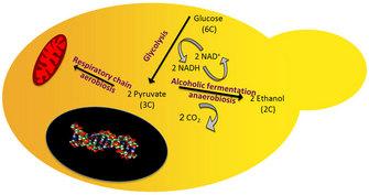
Yeastandothertypesofmicroorganismscanbeusedtobreakdownpyruvicacidinordertoproduce ethanol(Alba-Lois&Segal-Kischinevsky,2010).Aseukaryoticmicroorganisms,yeastsperform fermentationbyconvertingsugarintoalcoholthroughwhichtheyareabletoobtainenergy(Maicas, 2020).Yeastsandethanolfermentationareprimarilyusedtoproducebeer,wine,andotheralcoholic beverages, as well as bread (Helmenstine, 2020).

Duringethanolfermentation,pyruvateisbrokendownintoethanolandcarbondioxide.Thenet chemical equation for this process and the production of ethanol from glucose is:

C6H12O6 (glucose) → 2C2H5OH (ethanol) + 2CO2 (carbondioxide)

Glycolysisofaglucosemoleculeproducestwomoleculesofpyruvicacid,whicharethenreducedtotwo moleculesofethanolandcarbondioxideunderanaerobicconditions(Malakeretal.,2020).Specifically, thisprocessofbreakingdownglucoseintoethanolinvolvesacarboxylgroupbeingremovedfromthe pyruvate,whichissubsequentlyreleasedascarbondioxide.Thisproducesacetaldehyde,atwo-carbon molecule,whichcausesethanoltobeformedafterNADHpassesitselectronstoacetaldehyde,thereby regenerating NAD+ (Khan Academy, 2021).

Chemical process of ethanol fermentation. (Wikipedia,2021)

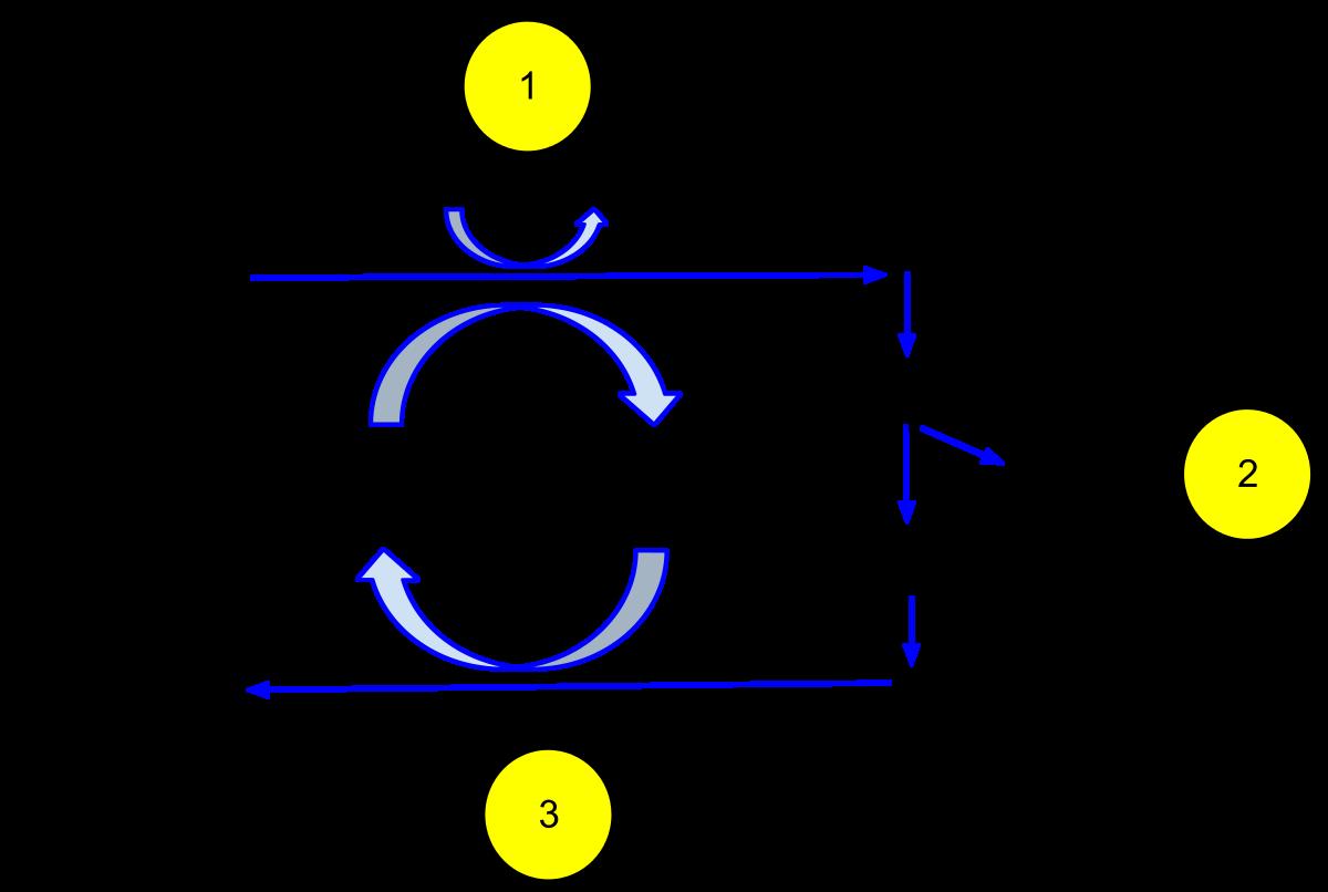
Sugarisoneoftheprimaryfactorsthatcanimpactandaffecttherateoffermentation.Inparticular,the concentrationofsugar,“increasesthefermentationproductioninyeast,untilthesaturationgradientis reachedcausingastopincarbondioxide,” andethanol(Bryanetal.,2018).Sugaraffectstherateof fermentationduetothefactthatitisaninputtocellularrespiration,andaidstheprocessofethanol fermentation.Specifically,yeastisafungus,meaningthatasupplyofenergyisneededforitslivingand growth(Hewitson&Hill,2018).Thisenergyrequiredbytheyeastissuppliedthroughsugar.Yeastisable toreleasetheenergyfromsugarduringfermentation,meaningthattheyeastismoreactiveifthereare highersugarlevels,andwillbefasterinitsgrowthuptoaparticularpoint(Hewitson&Hill,2018). Additionally,anincreasedlevelofsugarmeansthatthereisagreateravailabilityofthereactant,inthis case sugar, within the chemical reaction which thereby increases the rate of fermentation of yeast.

Hypothesis: Theyeastplacedintheliquidwiththehighestsugarconcentrationwillproduceagreater percentageofalcoholthanliquidswithlowersugarconcentrations,meaningthatitwouldhavethe highestrateoffermentation.Thiswillbeduetothefactthatthereisagreateravailabilityofthereactant in the chemical reaction in which alcohol is produced, thereby increasing the rate of fermentation.

Variables:

Independentvariable: Theindependentvariableinthisexperimentisthesugarconcentrationofthe liquids. This will be changed by using different types of fruit juices with differing concentrations of sugar.

Dependentvariable: Thedependentvariableinthisinvestigationisthepercentageofalcoholproduced duringfermentation.Thiswillbemeasuredusingatriple-scalehydrometer,whichmeasuresthespecific gravityofaliquid,whichistheratioofaliquid’sdensitytothatofwater.Fromthesemeasurementsof the specific gravity of the liquid the percentage of alcohol can be calculated.

Controlled variables:

● Volumeoffruitjuice:Thisvariablecanbecontrolledbyusingameasuringcylindertomeasure the same volume of fruit juice.

● Typeandmassofyeast:Thisvariablecanbecontrolledbyweighingtheyeastusinganelectronic scalebeforeplacingitintothefruitjuice,andensuringthatthesametypeofyeastisusedforall trials.

● Sizeofthecontainers:Thisvariablecanbecontrolledbyusingthesamesizeandtypeof containers for each trial.

● Amountoftimeoverwhichthedependentvariableismeasured:Thisvariablecanbecontrolled bybeginningeachtrialatthesameorverysimilartimeandensuringthattheamountoftime between the initial and final measurements of the dependent variable is the same for each trial.

Equipment and Materials:

● 300mL tap water

● 300mL unsweetened apple juice

● 300mL cranberry juice

● 300mL grape juice

● 24g baker’s yeast

● 1x triple-scale hydrometer

● 12x 500mL plastic containers

● 1x measuring cylinder

● 1x electronic scale

● 1x large test tube

Risk Assessment:

Potential Risk Precaution

Glass from triple-scale hydrometer causes cuts to hands and other body parts as a result of the triple-scale hydrometer being dropped.

Slipping and injuries to the body as a result of liquids spilling.

Handle the triple-scale hydrometer with caution, use the instrument correctly, and keep in the centre of the workbench to prevent it from falling or being pushed off. Use a dustpan to clean up broken glass in the case that the triple-scale hydrometer is broken.

Handle liquids with caution to prevent spillage, and ensure that they are in the containers at all

times. Keep containers in the centre/away from the edges of the workbench to prevent them from falling off. In the case that the liquids are spilled, immediately clean up safely using absorbent towels.

Method:

1.100mL of grape juice was measured and placed into a plastic container.

2.Step 2 was repeated twice; 100mL of grape juice was measured and placed into a plastic container, which was then repeated.

3.Steps 2-3 were repeated, with unsweetened apple juice, cranberry juice and water being used in place of grape juice.

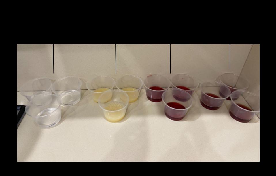
4.The initial specific gravity of each liquid was measured using a triple-scale hydrometer.

5.1g of baker’s yeast was added to each container containing the liquids.

6.The final specific gravity of the liquids in each container was measured using a triple-scale hydrometer six days after the initial specific gravity was measured.

7.The final percentage of alcohol of each liquid was calculated when the final specific gravity was subtracted from the initial specific gravity of each liquid, and then multiplied by 131.25.

Diagrams and photographs:

Measuring the specific gravity using a triple scale hydrometer

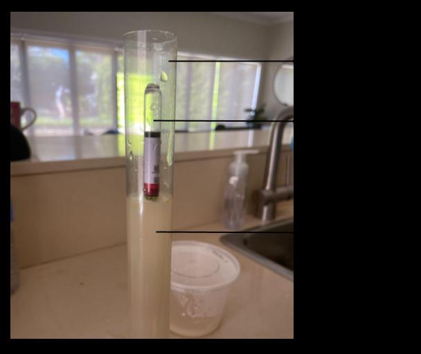
Results:

Table 1 - Initial specific gravity of each liquid:

Concentration of sugar (%) Initial specific gravity

Trial 1 Trial 2 Trial 3

0.0 1.000 1.000 1.000 10.8 1.046 1.046 1.046 11.3 1.046 1.046 1.046 13.7 1.060 1.060 1.060

Table 2 - Final specific gravity of each liquid:

Concentration of sugar (%) Final specific gravity of each liquid (after six days)

Trial 1 Trial 2 Trial 3

0.0 1.001 1.002 1.000 10.8 0.998 1.000 1.000 11.3 0.990 0.990 1.000 13.7 1.004 1.001 1.002

Percentage of alcohol of each liquid:

The final percentage of alcohol of each liquid was calculated using the following formula:

Percentage of alcohol (%) = (Initial specific gravity - Final specific gravity) x 131.25

Table 3 - Final percentage of alcohol of each liquid:

Concentration of sugar (%)

Final percentage of alcohol of each liquid (%)

Trial 1 Trial 2 Trial 3 Average

0.0 -0.132 -0.263 0 -0.132

10.8 6.300 6.036 6.036 6.124 11.3 7.350 7.350 6.036 6.912 13.7 7.350 7.740 7.613 7.568

Qualitative observations:

● Afewhoursaftertheyeasthadbeenaddedtoeachcontainer,eachliquidhadalayeroffoam, exceptforthewater,wheretheyeastremainedatthebottomofthecontainer.Thislayerof foam indicated that the yeast was active.

● Thefoamatthetopofeachliquiddecreasedsignificantlytwo-threedaysaftertheyeastwas addedtoeachcontainer,withthemajorityoftheyeastthatwasstillvisiblebeinglocatedonthe bottom of each container.

● Eachliquidsignificantlydiscolouredandbecamequitecloudythroughouttheexperimentin comparisontotheinitialcolouroftheseliquidsasaresultoftheaddedyeast.Inparticular,the water became a murky brown colour.

● Onthesixthdayoftheexperiment,theyeasthadnotfullydissolvedwithineachliquid. Additionally,asoftsubstancehadformedatthebottomofeachcontainerwhichwasparticularly noticeablewhentheliquidwaspouredintothetesttubesothatthefinalspecificgravitycould be measured.

Graphs:

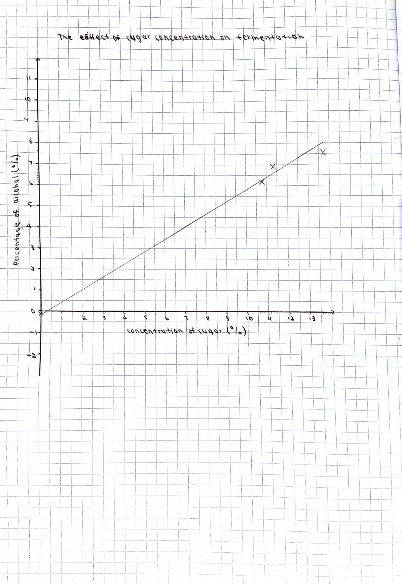
Figure 2: The effect of sugar concentration on fermentation (Excel graph)

Discussion:

Describing and explaining trends:

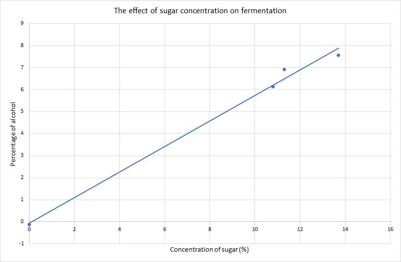
Theresultsofthisexperimentdemonstratethatliquidscontaininghighersugarconcentrationsproduce higherpercentagesofalcoholwhenfermentationwithyeasttakesplace.Thetrendshowninboth graphssupportsthis;theliquidthathadasugarconcentrationof13.7%(grapejuice),whichwasthe highestsugarconcentrationusedintheinvestigation,producedthegreatestaveragepercentageof alcohol,meaningthatithadthefastestrateoffermentation.Specifically,thepercentageofalcohol producedbythisliquidwas7.568%.Conversely,theliquidwiththelowestsugarconcentrationof0% (water)producedthelowestaveragepercentageofalcoholof-0.132%.However,thisvaluewas unexpectedinregardstothenegativevalueofthepercentageofalcoholproducedduringtrialsinvolving water.Inparticular,duetothefactthatthesugarconcentrationofthewateris0%,itwasexpectedthat thefinalpercentageofalcoholwouldbeequaltoorslightlygreaterthan0%.Additionally,anegative valueforthepercentageofalcoholisimpossibleasthisvaluemustalwayseitherbepositiveorequalto 0%.Notwithstandingthispossibleinaccuracy,theresultsoftheexperimentclearlyshowthathigher concentrationsofsugarproducehigherpercentagesofalcoholduringfermentationwithyeast,meaning thattherateoffermentationisfaster,asreinforcedbythepositivegradientofbothgraphswhich demonstratethatthereisastrongpositivecorrelationbetweensugarconcentrationandthepercentage of alcohol produced during fermentation.

Theseresultsandthetrendsshownthroughthedataandgraphsrelatetothebackgroundresearchof thisreportinregardstohowsugarconcentrationaffectstherateoffermentation.Inparticular,through thebackgroundresearch,itwasdiscoveredthatsugarisaninputtocellularrespirationand fermentation,andisareactantwithinthischemicalreaction,meaningthathigherconcentrationsof sugarwillproducegreaterlevelsofalcoholasaresultofthegreateravailabilityofthereactant(sugar). Thiscorrespondswiththeresultsofthisinvestigation,astheliquidwiththehighestsugarconcentration of13.7%(grapejuice)producedthegreatestpercentageofalcohol(7.568%)whencomparedtothe liquids with lower concentrations of sugar.

Evaluation:

Theresultsgainedandcollectedduringthisinvestigationwerereliable,asthreetrialsofeachchangeto theindependentvariablewerecompleted.Theresultsofeachtrialwere,forthemostpart,verysimilar. Hence,theresultsofthisexperimentwerereliableastherepetitionoftheexperimentproducedvery similarresults,however,theresultsofthisinvestigationwouldhavebeenmorereliableifthe experiment had been completed many more times.

Thisexperimentwasvalid,asthemethodinvestigatesandcollectsresultsregardingthepercentageof alcoholproducedduringfermentationwithliquidscontainingdifferentconcentrationsofsugar,whichis theaimoftheinvestigation.Italsousesthecorrectmaterials,successfullyaddressestheindependent anddependentvariables,andcontrolsthevariablesthatarerequiredtobeconsistentandcontrolled throughouttheexperiment,however,thereweresomeissuesinregardstoinconsistentmeasurements ofthemassoftheyeastplacedineachliquid,whichwasoneofthecontrolledvariables,asaresultof theinaccurateelectronicscalesusedtoweightheyeast.Thus,whiletherewereissuesinregardstothe accuracyofcertainequipmentandinstruments,thisexperimentwasvalidduetothewayinwhichthe method successfully tests the aim of this investigation.

Oneoftheprimaryproblemsthatwasfacedinthisexperimentwastheuseoftapwaterratherthan distilledwaterforthecontrolledsetupoftheexperiment,whichmostlikelyresultedinthenegative valueoftheaveragefinalpercentageofalcoholproducedduringfermentationwiththisliquid.This problemwouldhaveaffectedthemeasurementsandresultsofthesetrialsastheadditionalchemicals thatareaddedtotapwaterbywatercompaniescouldhavepossiblyaffectedtherateoffermentationas wellasthefinalreadings.Thisuseoftapwaterratherthandistilledwaterwouldhaveimpactedthefinal percentageofalcoholproducedduringeachtrialastheunknownchemicalspresentwithintapwater couldpotentiallyaffectandhindertherateoffermentation.Furthermore,anotherproblemthatwas encounteredduringthisexperimentwasthatthemassoftheyeastwasnotcontrolledacrossalltrialsas aresultoftheinaccuracyoftheelectronicscalebeingused.Inparticular,theelectronicscaledidnot recorddecimalplacesandoccasionallyhaddifficultypickinguptheweightofyeast,whichwouldhave thereforeaffectedtheresultsoftheexperimentasthemassoftheyeastusedduringeachtrialdiffered slightly.Hence,thefinalpercentageofalcoholproducedduringeachtrialwouldhavebeenaffectedby thedifferingmassesofyeastusedduetothefactthatgreaterorlesseramountsofyeastcanincreaseor decrease the rate of fermentation respectively.

Ifthisexperimentwastobecarriedoutagain,distilledwaterwouldbeusedinplaceoftapwatersothat thechemicalspresentwithintapwatercouldnotimpacttherateoffermentationduringthetrials involvingwater.Additionally,amoreaccuratescientificelectronicscalethatrecordsdecimalplaces wouldbeusedratherthanastandardkitchenscaleinordertoensurethatthemassoftheyeastis consistentandcontrolledthroughouteachofthetrials,therebyensuringthattheresultsofthe experiment are fair and accurate.

Conclusion:

Thehypothesisofthisexperimentwassupportedastheliquidswithhigherconcentrationsofsugar producedthegreatestpercentageofalcoholduringtheprocessoffermentationwhencomparedtothe liquidswithlowerconcentrationsofsugar.Thisisevidentthroughtheresultsoftheinvestigation,asthe grapejuice,whichhadthehighestsugarconcentrationof13.7%,producedthegreatestpercentageof alcohol,7.568%,whereastheliquidswithlowersugarconcentrationsproducedlowerpercentagesof alcohol during fermentation with yeast.

Reference list:

Alba-Lois, L. & Segal-Kischinevzky, C. (2010). Yeast Fermentation and the Making of Beer and Wine. Nature Education. 3(9).

https://www.nature.com/scitable/topicpage/yeast-fermentation-and-the-making-of-beer-14372 813/

Bryan, A., Hart, C., Wise, M. & Roberts, B. (2018). Glucose Concentrations Effect on Rate of Fermentation in Yeast. Journal of Undergraduate BiologyLaboratory Investigations. https://undergradsciencejournals.okstate.edu/index.php/JUBLI/article/view/8738

Helmenstine, A. (2020). What is Fermentation in Chemistry?

https://www.thoughtco.com/what-is-fermentation-608199

Hewitson, J. & Hill, C. (2018). How Does Sugar AffectYeast Growth?

https://www.saps.org.uk/saps-associates/browse-q-and-a/169-q-a-a-how-does-sugar-affect-yea st-growth

Khan Academy. (2021). Fermentation and anaerobic respiration.

https://www.khanacademy.org/science/ap-biology/cellular-energetics/cellular-respiration-ap/a/ fermentation-and-anaerobic-respiration

Maicas, S. (2020). The Role of Yeasts in Fermentation Processes. Microorganisms. 8(8). https://www.ncbi.nlm.nih.gov/pmc/articles/PMC7466055/

Malakar, S., Kr Sanjib, S. & Jolvis Pou, K.R. (2020). Biotechnological Interventions in Beverage Production. The Science of Beverages. https://doi.org/10.1016/B978-0-12-816678-9.00001-1

Tay, A. (2019). The Science of Fermentation. https://www.labmanager.com/insights/the-science-of-fermentation-1432

Warnant, P., Arena, P., Burrows, K., Lofts, G., & Evergreen, M.J. (2018). Jacaranda Core Science 5. John Wiley & Sons Australia.

Wikipedia. (2021). Ethanol fermentation. https://en.wikipedia.org/wiki/Ethanol_fermentation

Scientific Report - SRP - Maree Sialepis

Investigating the relationship between different colour noises and the amount of deep sleep they stimulate

Aim: To investigate the effect of pink, brown andwhite noise on the duration of deep sleep found through a percentage of overall sleep.

Background Research

Deep sleep allows the brain to effectively store memories and information as well as affecting its ability to recall information (Medical News Today, 2019). According to Suruchi Chandra M.D Integrative Psychiatry and Medicine (2021), “During sleep, ourbrains produce slower brain waves that allow the body and brain to enter a state of rest and restoration. There are fewer of the faster brain waves that occur during periods of focus and concentration.’’ Colour noises are able to amplify the slow rate at which the brain waves travel, stimulating more deep sleep. When brain waves slow down, this is accompanied by a relaxation of muscles including the eyes. Heart rate, blood pressure and body temperature will also decrease resulting in an overall better sleep. Through my proposed investigation, I will be able to uncover if colour noise really does reap the benefits of increasing or at least bringing deep sleep to a healthy level in individuals or perhaps if brown or white noise produces better results. Through this, I can promote the use of the most effective colour noise, something extremely accessible to the general public that can promote high quality sleep and brain functioning.

Neha Pathak, a doctor of medicine (2020), states that, “Pink noise is a constant sound in the background. It filters out things that distract you, like people talking or cars going by, so they don’t interrupt your sleep. You may hear it called ambient noise.” Pinknoise achieves this through its constant and steady frequency or pitch which creates a flat, even sound like rain or tidal waves. Doctor Michelle Drerup confirms that, “The pink noise actually enhances brainactivity that’s associated with deep phases of sleep.” This is because pink noise is a spectrum offrequencies whether the power per hertz decreases in intensity at a rate of 3 decibels per octave whilst the frequency increases simultaneously. As a result, “the lower frequencies in pink noise are louder and have more power than the higher frequencies” (Castro, 2013). The body also feels comfortable when listening to it because it changes in equal octave intervals. This constant decrease in sounds mimics natural rhythms of the body such as heart beating.

Brown noise is described to be deeper than pink and white noise. These soothing, lower frequencies may stimulate slower brain waves and thus produce deeper sleep. According to Dr Axe (2020), “Brown noise is considered a layered sonic hue that has a sound like a low roar.” The power of brown noise decreases as frequencies increase.. “Some report thatbrown noise serves as the perfect soft, monotonous soundtrack to life...brown noises can also be used to boost relaxation and focus. Continuous, soft noise can be used to help “quiet your mind” and tune out thoughts that may be running through your head.” This instant relaxation of thebrain and muscles is essential to stimulating deep sleep. White noise is a sound that contains all bands of frequency just as the colour white contains all colours of the spectrum. White noise has flat spectral density meaning that it is a signal that has equal power at different frequencies. The monotony and ‘one sound’ produced by white noise is proven to “help people who suffer with tinnitus and people who have trouble sleeping. That is because our brain can determine a single source frequency, but it becomes difficult to hear multiple” (Bazoyan, 2020). Thus, the continuity and stable nature of white noise does contend as an effective colour noise that can slow down brain waves and contribute to the stimulation of deep sleep.

Hypothesis:

I hypothesise that white noise will promote longer deep sleep because it contains all bands of frequency. This means that it is more effective in masking a variety of frequencies in sounds (ranging from 20 Hz to 20 000 Hz) that could disrupt the brain’s process in entering the deep sleep phase.

Variables in your investigation

Independent Variables Dependant Variables

Colour noise The duration of deep sleep as a percentage of overall sleep

Controlled Variables

The duration of colour noise being played - -

The time at which the subject prepares for sleep and wakes up - -

The volume of the colour noise - -

The distance of the audio device from the head of the subject - -

The diet and interactions of the subject - -

The room temperature - -

The amount of light within the room

Equipment and Materials

-Fitbit watch and app

-Audio device

-30 mins of white, brown and pink colour noise (provided by an audio device)

-Appropriate place to sleep

Risk Assessment

Risk Precaution

The subject may feel at discomfort with listening to the sound.

The subject may struggle with maintaining a constant diet or experience digestive issues.

In this unlikely case, choose another subject.

Ensure that the diet does not need to be the same each day but rather typical with no fluctuations caused by consumption of caffeine, excess sugar etc.

The subject’s typical and natural sleep patterns may be disrupted leading to mood/health problems.

The Method

If discomfort in sleep patterns causes extreme impacts, select another subject.

1.Prepared the subject for sleep at 11:00pm, ensuring they were in a comfortable position.

2.Ensured no air conditioning was on and only one small lamp outside the room was on.

3.Situated the audio device (phone) approximately 50cm away from the subject’s head.

4.Ensured the subject was wearing the fitbit device.

5.Played the first colour noise audio for 30 minutes.

6.Woke the subject up at 8:30am using an alarm clock.

7.Checked the statistics on the Fitbit application and recorded the percentage of deep sleep results into a table of results.

8.Repeated the experiment 3 days in a row with the same colour noise.

9.Repeated the experiment for another 3 days for a different colour noise, and then repeated for an additional 3 days using another colour noise. Results:

Quantitative Data:

Through observation of myself and my experience with the colour noises, I found that the pink noise did feel comforting and settling, seeming as though it changes in equal octave intervals so the stability of the sound may enable a sense of relaxation. The pink noise was also powerful enough to filter out the surrounding sounds but not to the point where it was a disruption to my body’s process in shutting down and calming down thoughts. The brown noise on the other hand was quite low and soft which meant that it was ineffective in blocking surrounding sound. The weakness of it may have affected its ability to slow down the speed of brain waves. White noise however was deemed, from an observational perspective, the most effective in putting me to sleep. This is because white noise is the auditory equivalent to white light, meaning it includes every frequency so even the smallest disruptive sounds can be masked, regardless of their frequency.

(sample screenshots of experiment)

Processing and Analysis of Results Graphs

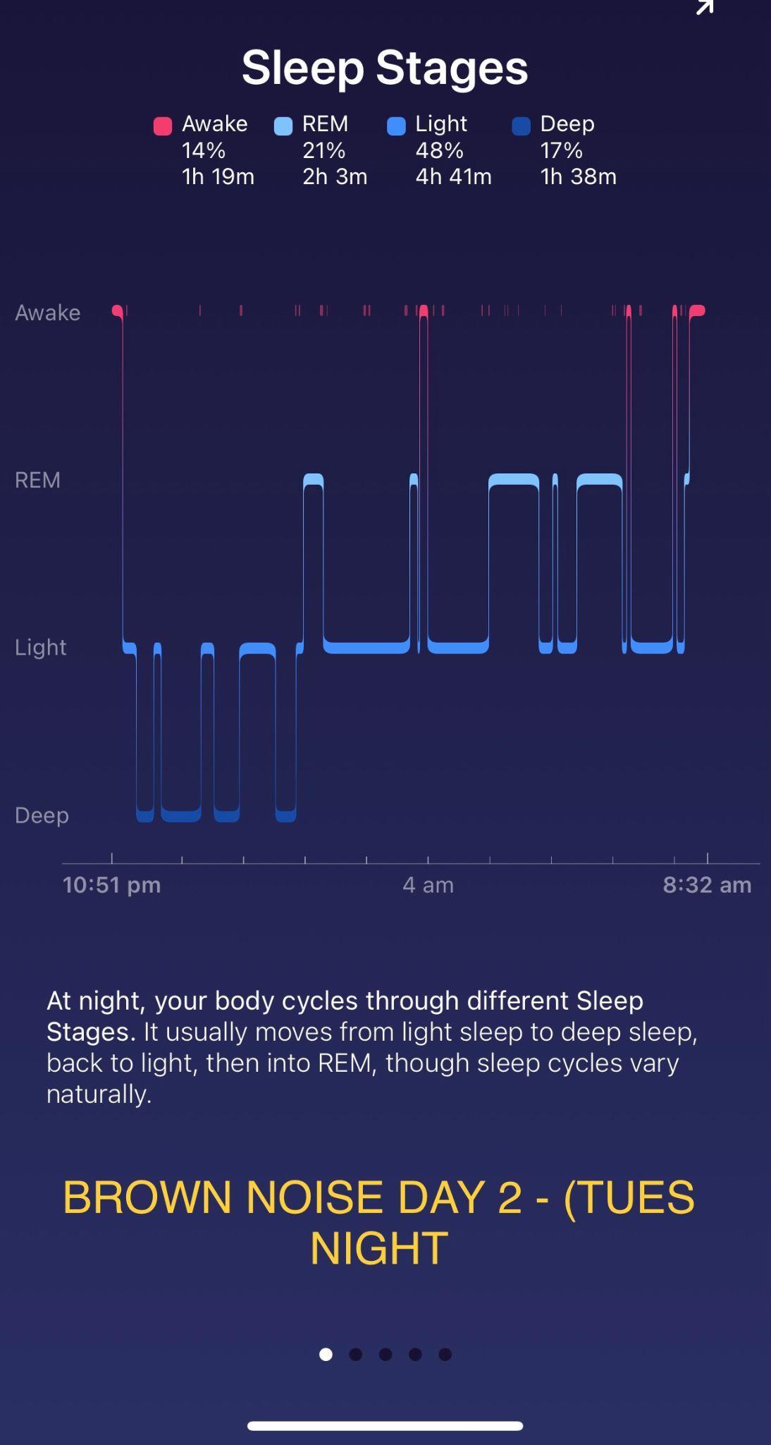
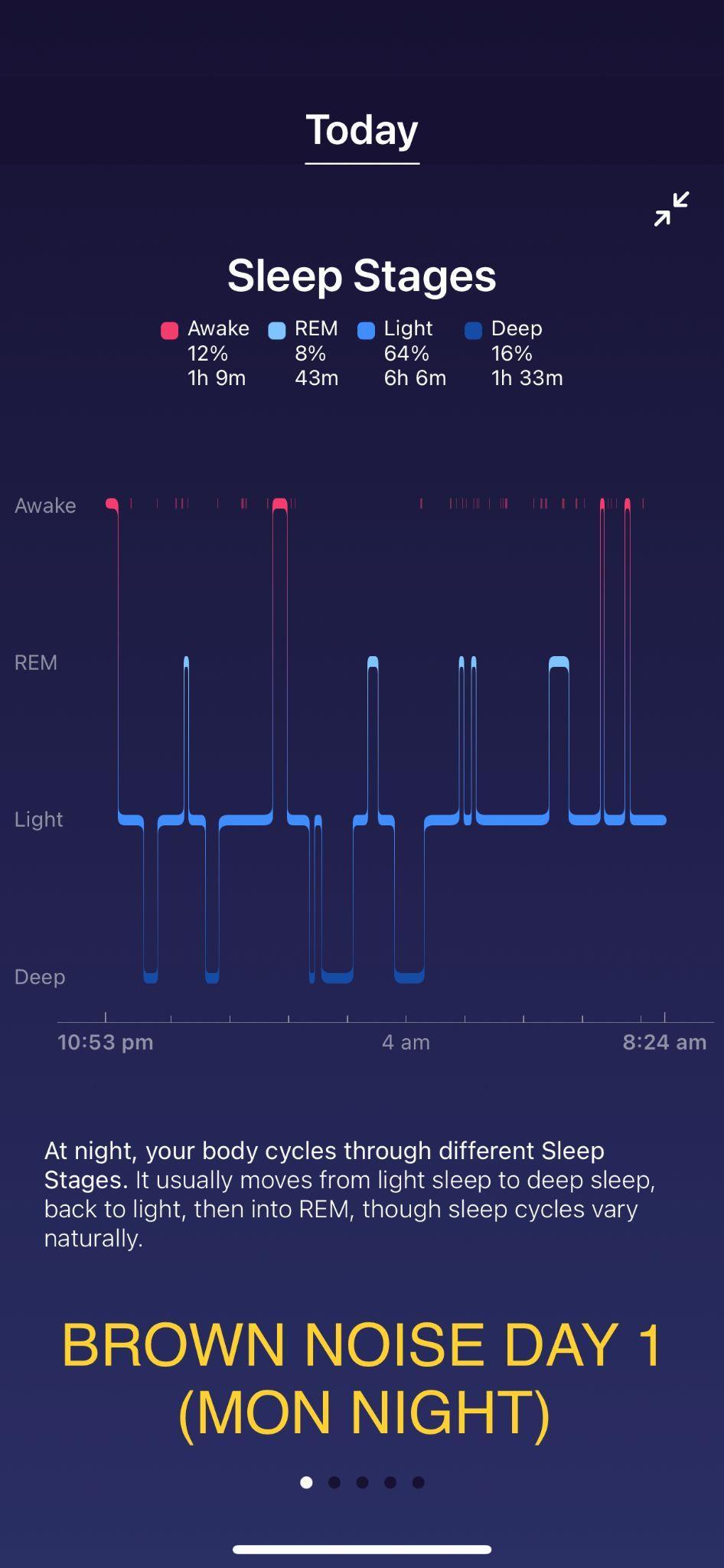
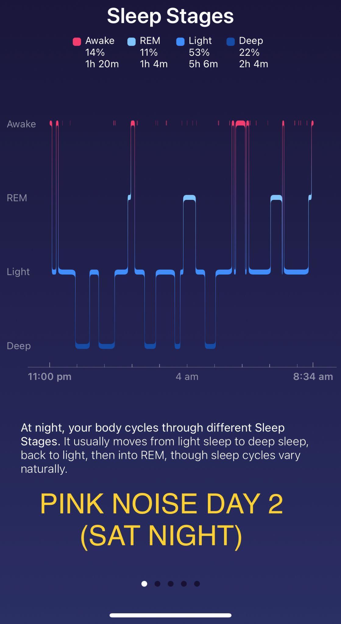
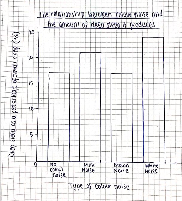
FIGURE 1

FIGURE 2

The Discussion

Describing and Explaining Trends

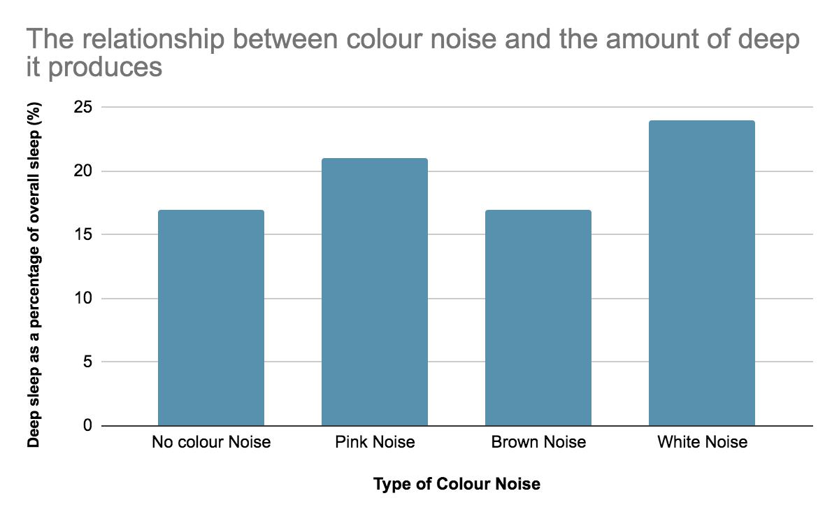
An evident feature found within the results is that white noise was the most effective colour noise for inducing deep sleep in comparison to brown noise which had close to no effect and pink noise which was successful but still did not produce as much deep sleep as white noise. White noise produced an average of 24% which was 7% more than usual deep sleep levels. Additionally, brown noise had no effect on deep sleep at 17% and pink noise produced slightly better results with an average of 21%. A trend found within the results was that white noise was more effective than pink and brown noise because it is a sonic embodiment of every frequency. This means it can range from 20 Hz to 20 000 Hz that fire off at random times throughout with equal power. White noise is also more effective than pink noise because it features frequencies that are both high and low whilst pink noise only features lower frequency sounds. This variety of frequency means that white noise is more successful in blocking out a range of different sounds produced by the subject’s environment. It prevents random and unprecedented inconsistencies in sound from disturbing the brain and thus deep sleep. In isolation of brown and pink noise, pink noise is deemed more effective because its lower frequencies are louder than the higher frequencies meaning the sound is less abrasive. However, although brown noise does have stronger and louder low frequencies this can be excessive and the deep sound may be too ‘rough’ or deep for the human ear and brain thus disrupting the body’s process in reducing the speed of brain waves.

Evaluation

I ensured my experiment was reliable by repeating it 3 times for each colour noise and finding an average in the results. However, in order for this reliability to be present the results despite being repeated, needed to be similar which is what I indeed achieved. Across my trials I found a 1-2% difference in results.

In order to receive valid results and ensure the experiment itself was conducted with validity, multiple variables were controlled resulting in a controlled environment. In attempting to achieve this, I went to bed at the same time each night and woke up at the same time with a 5-10 min leeway. It was also ensured that the same amount of light came through the bedroom, the colour noise played for 30 mins each night at the same volume, room temperature remained constant, my daily routine and diet remained relatively constant and the subject slept in the same place. Despite this, there was some difficulty in controlling the wake up and sleep time variables considering I did not have total control over what time my brain would go into a sleep phase thus I applied a 5-10 minute leeway which could have interfered slightly with my results although they were considerably consistent. In terms of measurement technique, my results relied on the fitbit tracking device. Although the source is extremely reputable and scientifically proven, I could only rely on my visual and auditory observations to a limited extent meaning any error derived from the results would be from the form of measurement. Furthermore, the amount of deep sleep was calculated as a percentage of overall sleep rather than based on hours as I didn’t want external factors such as the

amount of REM or Light sleep to impact the amount of hours of deep sleep. This thus looked at the data as a ratio rather than an isolated value.

The main error lies in the reliability of the fitbit watch itself. The watch relies on a combination of movement, heart rate and oxygen level patterns to determine the stages of sleep entered by the body. It also uses heart rate variability as this fluctuates depending on when the body enters deep, REM or light sleep. Despite the detailed collection of data being considerably accurate and reliable, complications such as movement of the watch on the wrist could have interfered with the fitbit monitor’s recording of this information. However, this is something that cannot be controlled in the experiment but would affect the results to a minor degree.

A second source of error that lied within the experiment is the control of diet and stress levels. This is yet another variable that could not be controlled due to the fact that the experiment was not conducted in an isolated laboratory but rather a normal environment where I, the subject, could not avoid undergoing certain events such as changes in diet (although not drastic), participating in exams, sports etc. These are compulsory events that I had to partake in which could have influenced the results. However again, the results only differentiated by 1-2% thus this error wouldn’t have had an immense influence.

In order to modify my experiment, I would ensure that the subject could, if possible, maintain a very similar diet over the course of the testing and undergo the experiment at a time where there were no ‘events’ that could impact stress, heart rate levels, mood or food/beverage consumption. I would also perhaps find a way to ensure that the fitbit watch results were reliable by using an additional different sleep tracking device beforehand to compare if the results obtained are similar and thus reliable.

Conclusion:

In the experiment, the relationship between different colour noises of pink, brown and white and the deep sleep they produced as a percentage of overall sleep was investigated. The results obtained support the hypothesis that white noise would be most effective in producing the most deep sleep. Its range of frequencies allow it to more successfully ‘mask’ or ‘block out’ external sounds of the environment that could thus disrupt the reduction of brain wave activity/speed.

APA Reference List

Bazoyan, A. (2020). White Noise and Other 5 NoiseColors. Krisp. https://krisp.ai/blog/did-you-know-that-noise-has- a-color/

Britannica, T. Editors of Encyclopaedia (2013). Noise. Encyclopedia Britannica. https://www.britannica.com/science/noise-acoustics#ref894665

Capritto, A. (2019).The secret to better sleep: Pink,Black, Blue and Brown noise. CNET. https://www.cnet.com/health/sleep/white-noise-pink-noise-blue-noise-brown-noise/

Castro, J. (2013). What is Pink Noise? Live Science. https://www.livescience.com/38464-what-is-pink-noise.html

Chandra, S. (2021). Pink Noise For Better Sleep, Memory& More. Suruchi Chandra Integrative Psychiatry /////& Medicine.https://www.chandramd.com/blog/pink-noise-benefits-sleep-memory

Health Essentials. (2018). Why "Pink Noise' MightJust Help You Get a Better Night's Sleep. Cleveland /////Clinic.https://health.clevelandclinic.org/why-pink-noise-might-just-help-you-get-a-better-nights-slee

Johnson, J. (2019). What to know about deep sleep. Medical News Today. https://www.medicalnewstoday.com/articles/325363

Johnson, G., Losos, J., Mason, K., Singer, S., Raven, P. (2010). Biology Ninth Edition. McGraw Hill.

Levy, J. (2020). What is Brown Noise? Benefits + Howto Use it for Better Sleep. Dr Axe. /////https://draxe.com/health/brown-noise/

Robinson, K, M. (2020).Pink Noise: Can it Help YouSleep? WebMD. https://www.webmd.com/sleep-disorders/pink-noise-sleep

Silver, N. (2020).How Long Does It Typically Taketo Fall Asleep? Healthline. https://www.healthline.com/health/healthy-sleep/how-long-does-it-take-to-fall-asleep

HS - Chemistry IA - FINAL

by Hannah Svoboda

Submission date: 02-Jun-2021 07:27PM (UTC+1000)

Submission ID: 1598939033

File name: HS_-_Chemistry_IA_-_FINAL.pdf (2.32M)

Word count: 6340

Character count: 31447

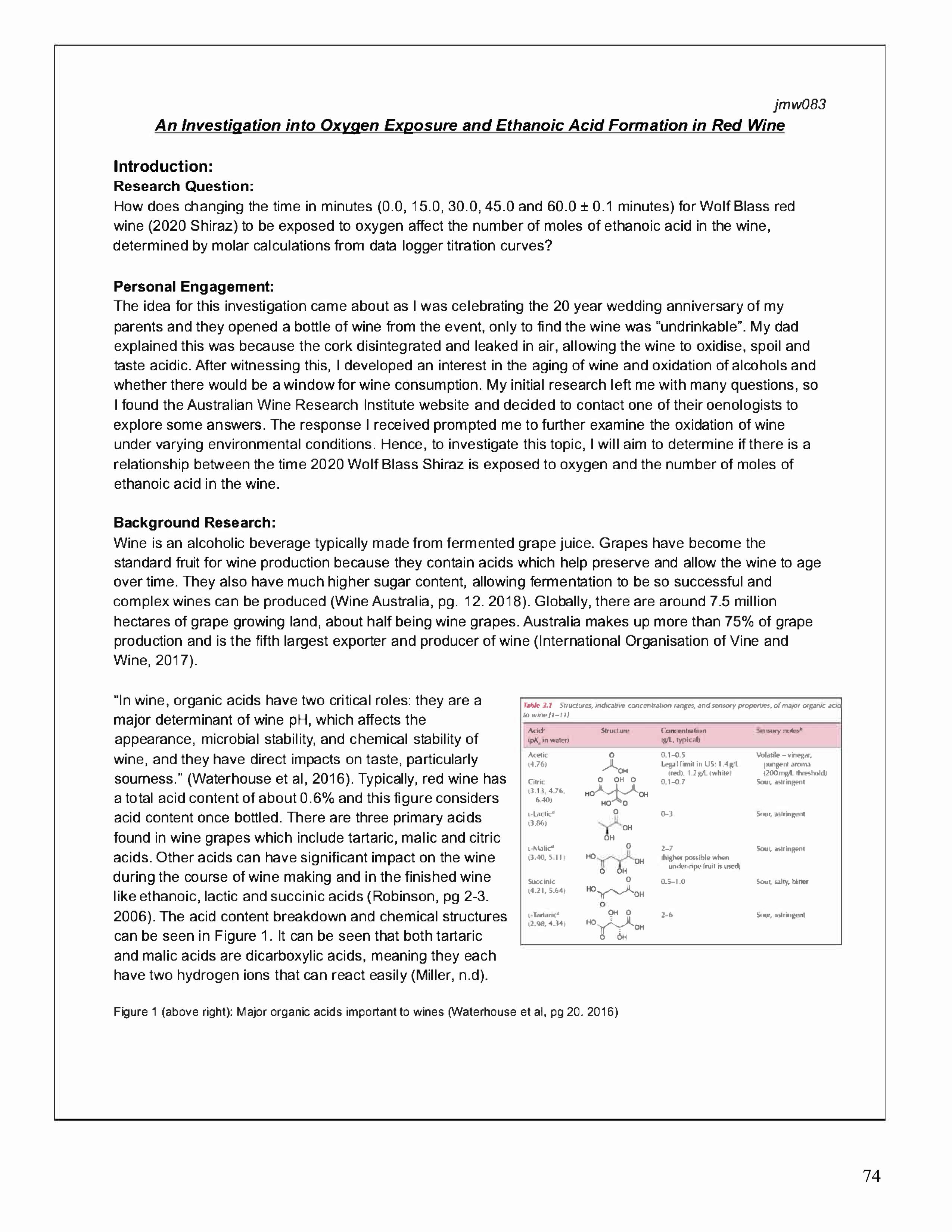
jmw083 Alcohols are organic compounds containing the hydroxyl (-OH) functional group, directly bonded to carbon. The carbon which is directly attached to the OH is referred to as the "carbinol" carbon (Ashenhurst, 2021), which can be seen in red on the ethanol structure in Figure 2. However, it is this carbinol carbon that is key to understanding common classifications used for alcohols, including "primary", "secondary" and "tertiary" alcohols (Ashenhurst, 2021). The names of alcohols can also be identified through their suffix '-ol'. To conclude the classification of an alcohol, the carbinol carbon must be examined: if it is attached to "one carbon, the alcohol is primary; two, secondary etc."

Ethanol is a simple primary alcohol with the molecular formula C2H5OH and the primary intoxicating ingredient of many alcoholic beverages including beer, wine, and spirits (Encydopaedia Britannica, 2019). A highly water-soluble liquid at room temperature, ethanol is also widely used as a solvent in cosmetics and pharmaceuticals (Pearson Chemistry 12 - New South Wales, 2019). The oxidation of primary alcohols, like ethanol, is a two stage process where an aldehyde is produced first, followed by a carboxylic acid. Any primary alcohol follows the sequence of oxidation seen in Figure 2.

H H I I +!OJ.heat H -f'o +!OJ heat reflux

H C C +!OJ.heat ----->

cth.Jn..il aldehyde cthanal aldehyde

H +!OJ.heat -----> n-flux

H C C H 011

cthanoit:u;:id arboxylic .acid ethanoicacid carboxylicacid

H -f'o H C C OH I H H c1hano primaryalcohol ethanol primaryalcohol

Figure 2: Ethanoicacid formation from the oxidation of ethanol, with intermediate ethanal (Brown, & Ford, pg505. 2014)

Ethanol is oxidised to ethanal which can be viewed as oxidation by removal of hydrogen, evident in Figure 2. For ethanoic acid to be formed, the aldehyde, in this case ethanal, must remain in the reaction mixture to oxidise for a longer period of time, essentially requiring a complete oxidation of ethanol. Ethanol also undergoes bacterial oxidation to form ethanoic acid. This form of oxidation is a problem for wine producers as air contains a large proportion of bacteria called Acetobacter, which use atmospheric oxygen to oxidise ethanol in wine, producing a weak solution of ethanoic acid. When a bottle of wine is exposed to oxygen in the air, bacteria slowly oxidise the ethanol to ethanoic acid, in extreme cases oxidising all of the ethanol into vinegar. Although ethanol is less reactive than other phenolics (chemical compounds consisting of one or more hydroxyl groups bonded directly to an aromatic hydrocarbon group [Swanson, 2003]), its high concentration in wine makes it a significant competitor in the oxidation-reduction potential medium when strong oxidants are present or the length of time to oxidise is extended (Margalit, 2016).

Ethanoic acid (CH3COOH) is the main volatile acid in wine. The term 'volatile acidity', or VA, is used to define a number of acids in this group. According to Victoria Burt, of the Wine & Spirit Education Trust (WSET), volatile acidity can be caused by "ethanoic acid bacteria, inadequate levels of sulfur dioxide, and excessive exposure to oxygen." (Clark, 2019). Sulfur dioxide, or SO2 , is an approved wine additive and used often as a preservative. Chemicals such as acetaldehyde can be added to wine, binding to the sulfur dioxide and making it unavailable as an antioxidant, hence the wine is available to oxidise.

This investigation will aim to determine ethanoic acid concentrations in red wine as the high ethanol content allows for higher concentrations of H+ ions to be detected through the complete oxidation of the alcohol. Sodium hydroxide (NaOH) will be used as a strong base and titrated against the weak ethanoic acid

jmw083 (CH3COOH) of the red wine, represented by the first equation below where the reactants are in a 1:1 molar ratio The secondequation represents the conjugate acid/base pairs:

CH3COOH(aq) + NaOH(aq) "'- NaCH3C00(aqJ + H20{IJ

CH3COOH(aq) + H20(1J "'- CH3COO·(aqJ + H30+(aq)

The reaction of a carboxylic acid like ethanoic acid is reversible so the equation is written with equilibrium arrows. Ethanoic acid is classified as a weak acid hence it only partially dissociates in water to form hydronium ions.

Titration curves are graphs used in Chemistry which plot the volume of titrant (NaOH/strong base in this situation) against pH Generally, the initial pH of a weak acid is higher than a strong acid. The beginning of the curve only increases gradually because the solution acts as a buffer, continuing until the base overcomes the buffering capacity (Sohn & Thornton, 2019). The equivalence point sees the pH to be greater than 7 as seen in Figure 3 because all of the acid (CH3COOH) has been converted to its conjugate

Titntlonof• wHk acid with■ 1tton1 ban

-•poin1

'°

.&O base (CH3COO-). Figure 3 (above right): The titration of a weak acid with a strong base (Freyre, n.d [CC])

An increase in the production of ethanoic acid through the oxidation of wine would result in the same initial pH reading of the wine and therefore the same initial concentration of W ions. However, different concentrationsof the acid in the actual wine itself would be present given wine is not just H• ions, rather a very complex mix of chemicals in solution. The titration would hence see more base required to reach the equivalence point in the trials with lower oxidation times as the overall concentration of acid in the wine is decreasing with the W ions increasing (W ion concentration will be greater than the initial acid concentration and require less base for neutralisation).

Hypothesis:

The number of moles of ethanoic acid in the wine will increase as the time for exposure to oxygen increases because when the ethanol present in wine oxidises, it forms ethanoic acid.

Variables: Figure 4: Independent and dependent variables withjustification

Variable Information

Justification

Independent Time in minutes for The selected time incrementsin minutes (0.0, 15.0, 30.0, 45.0 and 2020 Wolf Blass 60.0 ± 0.1 minutes) will ensure the wine has a range of times to be Shiraz to be exposed to oxygen and tested to provide distinguishable results. exposed to oxygen These five increments testedwill include data from five consistent, precise trials to ensure reliability of the experiment.

Controlled variables: Figure 5: Controlled variables; method and reason to control

Control Method to Control

Reason to Control

Typeof Purchase the same brand Alcohol content varies between brands and typesof wine soitis winebeing and typeof winetouse for important toensureonly2020 Wolf Blass Shiraz will bebought tested alltests and trials. and tested.

Batchof Purchasing the same Usingthesamebatchof wine ensures constant: grapes; growing winebeing harvest of wine: this conditions; production; treatment; harvesting time; andsoilquality. tested experiment will beusing Hence, confidenceincreases that changesinacidlevelsof the 2020Wolf BlassShiraz wine after oxidationare related to the experimental aim.

Volumeof Use a25cm3 glasspipette Ensuresany aciditychangesareaccountedfor astheoxidationof wineused tomeasureout 25.000 ± ethanolin wine. Alsoallowsfor the volumeof wine to remain per trial 0.045cm3 of wineeach trial. controlled, hence molar calculations will be moreaccurate.

Beaker to Use the same 100cm3 Pyrex The sizeof beaker usedtocontain wine samples must remain contain glass beakers. constanttoensure thesame surfaceareaof wineisexposedto wine air, preventingany furtheroxidationduring thetitration.

Molarityof Use alabtechnician The molarityof the sodiumhydroxide (NaOH)solution must NaOH prepared 0.100mol sodium remain constant throughout trials toensure molar calculationsafter solution hydroxide solution the data is collected will beconsistent.

Volumeof Teacher will add, with a Tobest model the agingof wine, acetaldehyde will beadded to acetaldehyde pipette, 1.0 ± 0.1cm3of "bind sulfur dioxide, makingit unavailableas an antioxidant" so added to acetaldehyde to eachlarger oxidationmayoccur (Cordingley, B.[Personalcommunication wine beakerof wine. (email)].November25, 2020).

Air stone/ The AquaOne 500 air Air will bebubbledinto the wine usingan air stone to get alarger pipe stone, pump and pipe gas/liquidinterface. This models oxidation of wine over time and diameter diameter will be used. allows results to beobtainedover theexperimental period.

PASCOpH Use the samePASCO No needtoconsider varying calibrationsof the equipmentif the probe digitalpH probe each trial. same probeis used for all trials.

Temperature/ Conductedonthesame "Anincreasein temperature typicallyincreases rateof reaction" locationof bench with temperature and (Key, 2020)sothiscontrolensuresonlyoxygen exposuretime experiment anomaliesmonitored. affects acid levels, eliminating environmental interference.

Confounding variables:

• Thewine may continuetooxidise withthe air during the titration, afterpumping with the aquarium bubbler.Thiscouldthereforeleadtosome ethanoicacidformation after the set time planned (0.0, 15.0, 30.0, 45.0 and 60.0 ± 0.1 minutes)for thewinetooxidise

• If two bottlesof the same wineareneededfor the experiment duetothenumberof trials conducted, onemayhave aslightly higher concentrationof ethanol for acidformation, even if they were produced under the sameconditions

• Theambient temperaturein thelabmay fluctuate over the five day periodthe experiment was conducted duetovarying weather inthelocationof the lab

Equipment Uncertainty Purpose

15x 100cm3 ± 10cm3 Usedtocontain the 25 ± 0.045cm3 ofredwine foreach trial underthe beakers burette fortitration against the sodiumhydroxide. Conical flaskscouldnot be used dueto also needing to place the pH probein the solution.

20.0cm3 ± 0.1cm3 Acetaldehydeisneededin thisexperiment to "bind sulfur dioxide, makingit acetaldehyde unavailable as anantioxidant" (Cordingley, B. [Personal communication (email)]. November25, 2020), hence oxidation can occurat a faster rate.

2x bottles2020 N/A Usedas ageneralmodelforethanol conversioninto ethanoicacidinred Wolf BlassShiraz wine after oxidation. This wine is being chosen due to easy access to the product and noenvironmentalorethical concerns asit issourcedlocally.

1250cm3 X NaOH ± 0.001 mol Acts as the titrant in the experiment so that the concentration of acid in the solution (0.1oo mol) wine canbe calculated stoichiometrically

1xAquaOne 500 N/A Theaquariumpump andtube will aeratethebeakerscontainingwine to be aquariumpump, exposed to oxygen. Theairrock attaches to the tube and sitsat thebottom airrock, tube ofthe beaker, so aircanpumpthrough theentirevolumeofwine.

1x PASCO digital ± 0.01 pH Takes precisepH readingsin the titration, providing a data loggergraph to pH probe units display the equivalence point, and determine that value to record.

1x plastic pipette ± 0.1cm3 Usedby the teacher to add the volumeofacetaldehydeto the wine.

1x pipette filler N/A Usedtorelease airanddraw the wineinto the glass pipette safely

1x 25.000cm3 ± 0.045cm3 Needed to measurea constant and accurate volumeof the redwine into glasspipette thebeakers eachtrialforthetitration.

1x 50.00cm3 ± 0.05cm3 Contains the NaOH. The abilitytocontrolprecisionoverotherequipmentis burette beneficial for performing acid content molar calculations in the wine.

1x buretteclamp N/A Requiredto hold the burette level and securelyforthetitration.

1x retort stand N/A Support the burette clampand hold equipment at a comfortable height.

3 x 200.0cm3 ± 7.5cm3 To containeach test of the red winewhich will beexposed to oxygen beaker beforedividinginto smallerbeakersforthe trialsand eachtitration.

1x funnel N/A To safelypour NaOH solution into the burette, minimising spillage risk.

1x Fastime ± 0.01 Ensures the time the wineis left tooxidiseisequal tothat statedin the stopwatch seconds independent variable.

1x IEC magnetic N/A Usedtoensure that thesolutionofwine withbaseis mixedautomatically stirrerand bar whilethetitrationis occurring without the need formanual stirring.

Distilled water N/A To rinsethe pHprobeaftereachtrial.

RiskAssessment/Environmental and Ethical Considerations: Figure 7: Risk, environmental and ethical assessment, hazards and methods to minimise risk

Hazard Risk Method to Minimise Risk

Broken glass Cuts to skin

• Be careful when handling glass apparatus

• If glass breaks, alert teacher and clean up using dustpan, wrap in newspaper before putting it in the bin Do not use fingers

• Teacher use only a possible cancer risk

Acetaldehyde is Increased

• Do not ingest, inhale or come in contact with chemicals. Wear gloves, carcinogen goggles and a lab coat (PubChem, 2021)

Inhalation of Airway and

• Teacher use only, do not stand over or inhale the chemicals acetaldehyde lung irritation

• Should inhalation occur, contact Poisons Information Centre Australia

• Causes serious contact irritation and bums, teacher supervision or exposure irritation use.Immediately callmedical assistance if contact occurs

Acetaldehyde Skin and eye

Wine ingestion Allergic

• Wash hands after use and keep away from others while using reaction

• Do not drink to limit contamination or allergen spread

• Do not ingest chemicals, may cause abdominal pain (LabChem, 2018) NaOH solution irritation

Ingestion of Stomach

• If ingested, contact Poisons Information Centre Australia

• Dispose of acetaldehyde solution in chemical waste bin through lab disposal contamination technicians to avoid waterway contamination (IMAP, 2017)

End-product Environment

There are no ethical considerations as no animal or human subjects wereused in the investigation.

Method:

1) Gather all equipment and reagents. Put on a lab coat and goggles.

2) Open the bottle of Wolf Blass 2020 Shiraz and pour into a 200cm3 beaker

**Note: Steps 3-5 ofthis method do notneed to be completedfor thefirst test of0.0minutes±0.1 minute

3) Set up the AquaOne 500 aquarium pump, attach the tube and the air stone then place the air stone at the bottom of the beaker. The stone will ensure the tube remains submerged.

4) Teacher required to add 1 ± 0.1cm3 acetaldehyde to the beaker using a plastic pipette under a fume hood.

5) Turn on the aquarium pump and start the stopwatch for the time exposed to oxygen for each test (0.0, 15.0, 30.0, 45.0 and 60.0 ± 0.1 minutes) as stated in the independent variables table, Figure 4.

6) While the pump is bubbling air into the wine, set up the retort stand and burette clamp.

7) Rinse the burette with the prepared 0.100 mol NaOH solution into the sink.

8) Ensuring the stopcock is closed, fill the burette using a funnel with NaOH solution to the zero mark, with the bottom of the meniscus on the mark. Place the burette into a clamp on the retort stand.

9) After the time for the test reads on the stopwatch, turn off the pump and take out the air stone.

10) Use a 25cm3 glass pipette and filler to draw up 25 ± 0.045cm3 of wine from the beaker into a 100cm3 beaker and place under the burette tip on the magnetic stirrer, placing the stirrer bar in the beaker.

11) Turn on the PASCO digital pH probe and follow instructions to pair via Bluetooth to the SparkVUE app.

12) Place probe inside the beaker, ensuring a pH reading is visible on the screen.This probe replaces the need to use an indicator for equivalence point, considering wine is a coloured solution.

13) Begin to titrate the wine against the NaOH by twisting the stopcock open. The SparkVUE app is a data logger and requires the screen to be clicked for every 1cm3 of base added to the wine, creating the graph.

jmw083

14) Titrate the full 50 ± 0.05cm3 of NaOH solution to graph a full titration curve on the data logger. Export the trial for when the equivalence point will be determined at a later time and recorded in Figure 9.

15) Rinse the pH probe with distilled water over the sink and set aside.

16) Pour mixture of red wine and NaOH into a large waste beaker and move the beaker aside.

17) Repeat Steps 8 to 14 until 5 trials of the same test yield consistent data.

18) Repeat Step 15 for the remaining test times for the wine to be exposed to oxygen.

19) Clean up the lab bench and dispose of waste chemicals with lab technician assistance.

Justificationof Method:

This method was designed for accurate and reliable data collection through consideration like the chemicals and equipment used to convey and obtain results, trial repetition and general accessibility of the experiment. A total of five time intervals (0.0, 15.0, 30.0, 45.0 and 60.0 ± 0.1 minutes) for the wine to be exposed to oxygen will be tested, with each test repeated until five sets of consistent results are yielded. Equipment used like the PASCO digital pH probe and glass pipette have very low uncertainties of ±0.01 pH units and ±0.045cm3 respectively which increases the precision of the experiment. The method is accessible as materials can be sourced through a school laboratory with moderate testing times.

MeasurementUncertainties:

Figure 8: Measurement uncertainties table and considerations

Measuring Instrument Uncertainty Smallest Quantity Measured % Measurement Error

PASCO pH probe ± 0.01 pH units 3.77 pH units 0.265%

25cm3 glass pipette ± 0.045cm3 25.000cm3 0.180% 50cm3 burette ± 0.05cm3 25.40cm3 0.197%

Measurement uncertainties (Figure 8) should ideally be lower than 1% in Chemistry and a strength of this experiment is that the highest percentage measurement error is 0.265%, for the PASCO pH probe. This shows that the percentage errors of the measuring instruments and equipment used to collect the data for this investigation have been considered and are within an appropriate range to increase precision.

Data Collection and Processing:

Raw Data:

Figure 9: Raw data table of the volume of sodium hydroxide rnrated to reach the equivalence point± 0.05cm3 for all trials

Time for wine to be exposed Volume of NaOH titrated to reach the equivalence point± 0.05cm3 to oxygen± 0.1 minutes Trial 1 Trial 2 Trial 3 Trial 4 Trial 5 0.0 29.50 30.10 30.10 29.70 30.30 15.0 27.10 27.05 27.15 27.05 27.20 30.0 26.70 26.75 26.85 26.80 26.70 45.0 25.55 25.55 25.70 25.75 25.65 60.0 24.65 24.70 24.75 24.70 24.55

The raw data seen in Figure 9 was attained through a data logger on the SparkVUE app, which sourced data from the PASCO digital pH probe during the titration. Images/files of each titration trial for the data logger were exported and inserted into a software (WebPlotDigitizer) which found the equivalence point on the graph to two decimal places.

*Note: WebP/otDigitizersoftware source locatedin reference list

Processed Data: Figure 10: Processeddata table

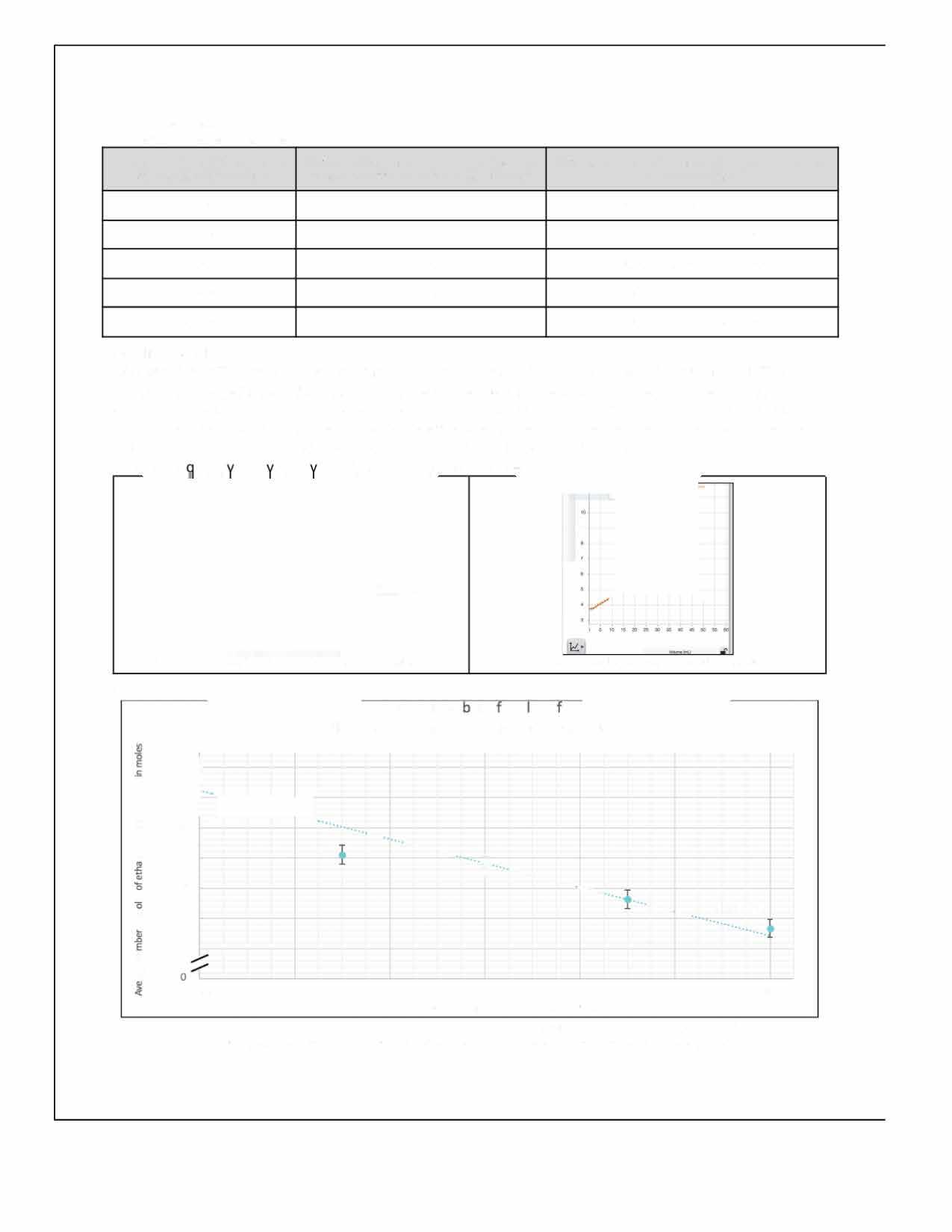
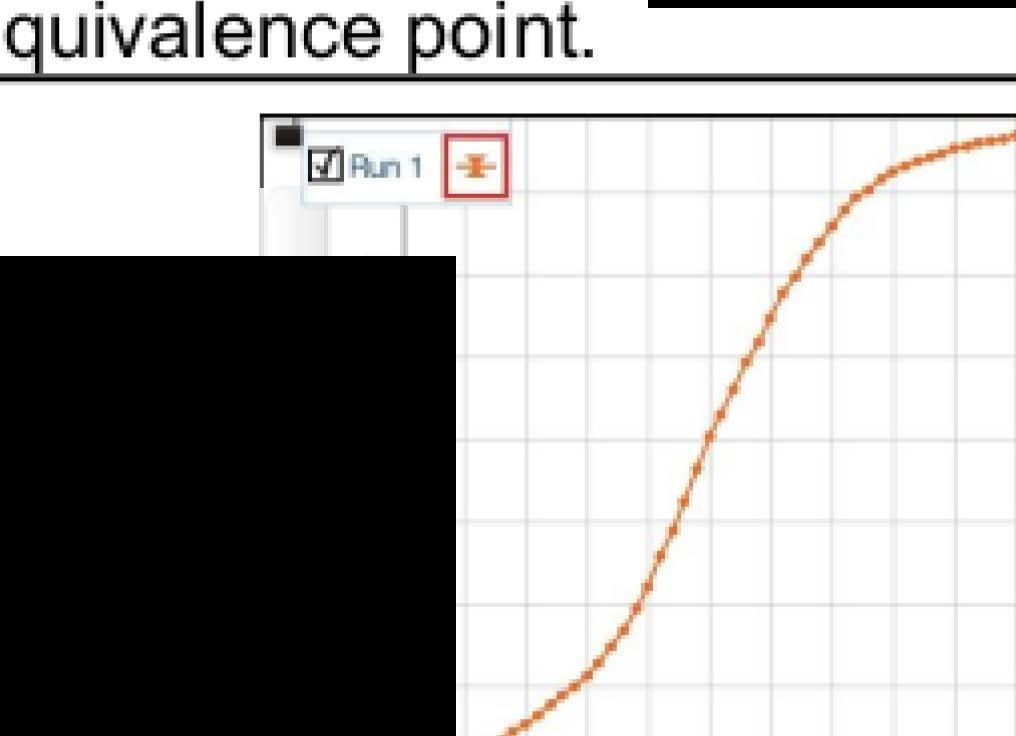
Time for wine exposure to Average volume of NaOH titrated to Average number of moles of ethanoic acid oxygen ± 0.1 minutes reach equivalence point ± 0.05cm3 in the wine (mol) 0.0 29.94

2.994 X 10" ± 3.494 X 1Q-5 15.0 27.11

2.711 X 10" ± 3.211 X 1Q-S 30.0 26.76

2.676 X 10" ± 3.176 X 1Q-5 45.0 25.64

2.564 X 10" ± 3.064 X 1Q-5 60.0 24.67 2.467 X 10" ± 2.967 X 1Q-5

QuaIitative/Photos:

Observations: The wine colour turned fromdeep red to green/blue once in a solution with NaOH. The odour also changed froma distinct alcohol-based wine scent to one similar to vinegar at the conclusion of each trial. The initial pH of the wine remained constant for all trials at approximately 3.77 ± 0.01 pH units. Photos: Figure 11 is anannotated photo of the experimental setup. Once prepared as per this image, the data logger was turned on and the trial could begin. Figure 12 displays the data logger graph which was then subse uentl anal sed b a software to determine the e . '

Figure11:Annotatedphotobyauthorofexperimentalsetup

Discussion:

Analysis:

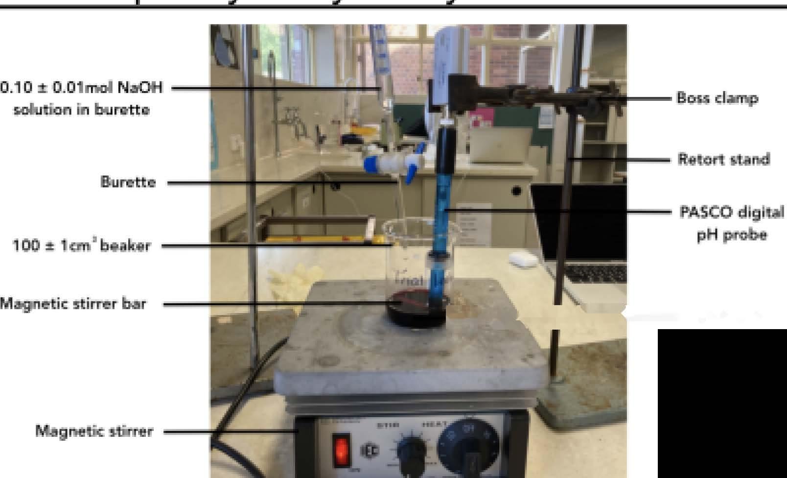
The data gathered from this investigation exploring the relationship between the time wine is exposed to oxygen and the levels of ethanoic acid in the wine shows a very strong, negative linear correlation, which can be observed in Figure 13. As the time for the wine to be exposed to oxygen increases, the average number of moles of ethanoic acid in the wine decreases. This decrease is also displayed in the processed data in Figure 10, as when the wine was exposed to oxygen for 0.0± 0.1 minutes, the average number of moles of ethanoic acid in the wine over five trials was 2.994 x 10 3± 3.494 x 10 5 mol, whereas when the wine was exposed to oxygen for 60.0± 0.1 minutes, the average number of moles of ethanoic acid was lower at 2.467 x 10 3± 2.967 x 10 5 mol. The vertical error bars on each data point in Figure 13 represent the absolute error propagated for each test, or the uncertainty of the average number of moles for each time interval the wine was exposed to oxygen. Therefore, higher uncertainty exists between the data points at the 15± 0.1 minutes and 30± 0.1 minutes tests as the error bars overlap. The R-value calculated from the data collected in this experiment was -0.9108. This value supports the very strong, negative linear relationship between the data points and is represented above the trendline in Figure 13. However, an outlier in the data existed at 15± 0.1 minutes of oxygen exposure with a value of 2.711 x 10·3± 3.211 x 10 5 mol and the R-value could have been closer to -1 (perfect negative correlation) if excluded from analysis or re-tested. It is unable to be exactly determined what caused this value to deviate from the expected trendline but it is likely to be attributed to a combination of the many listed errors in Figure 14.

Conclusion:

The results of this investigation revealed that as the time for the wine to be exposed to oxygen increased, the average number of moles of ethanoic acid in the wine decreased. The equivalence point differed between tests as seen by the average volume of NaOH required to titrate to the equivalence point± 0.05cm3 in Figure 10. There is a general decrease in the volume of NaOH required with 29.94± 0.05cm3 needed for the 0.0± 0.1 minutes test and 24.67± 0.05cm3 needed for the 60.0± 0.1 minutes test. The pH of the equivalence point remained greater than 7 for all tests because all of the acid (CH3COOH) was converted to its conjugate base (CH3COO ). This showed that the overall concentration of acid in the wine decreased as the H+ ions increased, because Wion concentration was greater than the initial acid concentration and required less base for neutralisation. These results are supported by the scientific understanding of reactions between weak acids and strong bases as detailed in the background information. Because ethanoic acid is a weak acid, it only partially dissociates in water to form hydronium ions and there is a buffer until the base (NaOH) overcomes the buffering capacity, hence the reaction is in constant equilibrium. Also, the reactants were in a 1:1 molar ratio which allows for the explanation that higher volumes of NaOH were required to neutralise the higher number of moles of ethanoic acid in the wine, seen when there was less time for the wine to oxidise. The percentage error could not be calculated for this experiment given the lack of theoretical values available. Despite extensive research and re-contacting the AWRI, no theoretical values which could be attained as a reference to this investigation, hence evidence as to whether the main sources of error were systematic or random cannot be produced. Generally, suggestions and ways to minimise error and improve the investigation are listed in Figure 14.

The experimental findings connect to industry in the properties and changes of wine under varying environmental conditions, such as oxygen exposure which was tested in this investigation. Winemakers often dedicate additional time into researching the chemical processes and importance of determining acid content in wine through methods explored similar to titration and molar calculations, better facilitating production, storage and consumption. Ensuring the consistency of these industrial processes is vital in winemaking as there are many internal and external variables for oenologists to understand and control.

Evaluationand Extension:

The purpose of this investigation was to explore if a relationship exists between the time 2020 Wolf Blass Shiraz isexposed to oxygen and the number of moles of ethanoic acid in the wine. The experiment had a number of weaknesses, limitations and errors which are all outlined in Figure 14, a table of systematic and random errors, their impact on the experiment and methods to eliminate these sources of error. As the data was collected over many days, one way to improve the overall precision in results would have been attempting to conduct all trials on the same day, where conditions inside the lab would be constant.

Although the experiment was quite reliable as the five trials completed yielded similar results (as seen in Figure 9), the range between these trials could always be further reduced through the additional improvements and minimised error methods in Figure 14. The investigation also had a high degree of validity as focus remained on the experimental aim, the hypothesis was supported and all controlled variables were kept. The precision regards the uncertainty and repeated measurements of a trial, which were outlined in both the measurement uncertainties table of Figure 8 and the processed data table of Figure 10. Percentage uncertainty of the mean for the test times the wine was exposed to oxygen (0.0, 15.0, 30.0, 45.0 and 60.0 ± 0.1 minutes) were all under 1.20%, where sample calculations can be found in the Appendix. The precision of the experiment was hence somewhat high, but should ideally be lowered to under 1% to be considered highly precise. In this case, the limitation of precision was due to measuring and calculating such small values of ethanoic acid formation in the wine, with 2.467 x 10 3 ± 2.967 x 10 5 mol (or 0.0024670 ± 0.0000297 mol) being the lowest value detected through calculation. This could be improved by exposing the wine to oxygen for longer periods of time so more distinguishable results may be obtained with further ethanol conversion to ethanoic acid. However, the overall impact of theseerrors is unable to be connected to accuracy as no literature values were obtained despite extensive research to calculate percentage error or determine how close the experimental data was to established values.

Some strengths of the investigation included: having a wireless, digital pH probe to indicate for the equivalence point; using a data logger to obtain a pH curve directly from the raw data; obtaining the equivalence point using the raw data from an accurate software; and the repetition of at least five, consistent trials per test. To extend this investigation, the experiment could be tested with:

• Longer periods of time for the wine to oxidise given wine spoilage often occurs over longer periods of time, allowing the wine to have longer oxygen exposure may give a moreaccurate indication of the relationship between oxidation time and ethanoic acid formation in wine

• Different ambient temperatures of the wine -to determine if other environmental conditions impact upon levels of ethanoic acid formation in wine, which could link to storage methods of wine

• A different wine variety (eg. Riesling, Pinot Grigio etc.) to Shiraz - allows comparison to be made between different types of wine to investigate any similarities or differences

Figure 14: Random and systematicerrors, effect on experiment and method to minimise impact

Error Detail Effect on Experiment

Method to Minimise Impact

Systematic Different bottles of Chemical concentrations could Error cannot be minimised as the wine wine used vary between bottles volumerequired isgreater thana bottle

Systematic Changes in acid CO2 may be dissolved in solution Consideration this error and as it may content of solution (in equilibrium with carbonic acid) causea larger range between trials

jmw083

Systematic Human error in AFastime stopwatch was used to Account for the human error by timing tests and time the wine aeration but human including an uncertainty in the time the turning off the error was involved in reacting to wine was exposed to oxygen of± 0.1 aquarium pump turn the pump off minutes (or 6 seconds)

Systematic Parallax error of The burette was set up very high Use a small step ladder to ensure reading the to compensate for the magnetic eye-level can be maintained with the burette stirrer hence eye-level could not meniscus of the burette or use a lower be maintained on the meniscus lab bench/desk

Random Calibration of the Lead to variance in interpretation Consistency in initial values should be pH probe may of the equivalence point for each checked with another probe. Lab have varied over trial, ultimately affecting the values technicians to assist in recalibrating the the trial duration in Figures 9 and 10 probe each day if needed

Random Varying ambient Change in temperature across the Note all fluctuations in temperature in conditions over days the experiment was the lab over the period the experiment the duration of the conducted may have led to slightly was conducted or attempt to conduct all experiment varying reaction rates trials during the same day

Random Distraction of the The experimenter had to use Ensure others in the room know that experimenter complete focus while using the concentration is required during trials, when using the data logger by clicking for each limit external distractions and redo any data logger 1.00± 0.05cm3 that the meniscus trials which were influenced by passed along the burette distractions or misclicks

Random Magnetic stirrer This resulted in the stirrer stopping Re-start any trials where the stirrer bar bar getting caught mid-trial so the solution would not gets caught in the beaker to allow for on pH probe be thoroughly mixed consistency in data collection/method

Reference List:

Ashenhurst, J. (2021). Alcohols (1) Nomenclatureand Properties. RetrievedFebruary 17, 2021, from https://www.masterorganicchemistry.com/2014/09/17/alcohols1nomenclatureandproperties/ Brown &Ford. (2014). ChemistryfortheIB Diploma. (2014 edition). Oxford: Oxford University Press. Retrieved February 28, 2021.

Cordingley, B. [Personal communication (email)]. November 25, 2020. Encyclopaedia Britannica. (2019). Ethanol. RetrievedFebruary 1, 2021, from https://www.britannica.com/science/ethanol

IMAP. (2017). Acetaldehyde: Human health tier II assessment. Retrieved February 13, 2021, from https://www.industrialchemicals.gov.au/sites/default/files/Acetaldehyde_Human%20health.pdf

International Organisation of Vine and Wine. (2017). 2017 World Vitiviniculture Situation. Retrieved March 1, 2021, from https://www.oiv.int/public/medias/5479/oiv-en-bilan-2017.pdf

LabChem. (2018). Sodium Hydroxide, 0.1N (0.1M) Safety Data Sheet. RetrievedFebruary 13, 2021, from http://www.labchem.com/tools/msds/msds/LC24270 pdf

Margalit, Y. (2016). Concepts in Wine Chemistry. (third edition). USA: Wine Appreciation Guild. Retrieved February 1, 2021.

jmw083 Miller, M.(n.d). MonitoringAcids and pH in Winemaking. Retrieved February 11, 2021, from https://www.accuvin.com/wp-content/uploads/2015/04/MonitoringAcidsandpHinWinemaking.pdf

PubChem.(2020). PubChemCompound SummaryforCID 177, Acetaldehyde. Retrieved February 23, 2021, from https://pubchem.ncbi.nlm.nih.gov/compound/Acetaldehyde

Robinson, J.(2006). The Oxford Companion to Wine.(third edition). Oxford: Oxford University Press. Retrieved February 23, 2021.

*Rohatgi, A.(2020). WebPlotDigitizer. Retrieved April 17, 2021, from https://automeris.io/WebPlotDigitizer/index.html

Sohn, H & Thornton, J.(2019). Titrations of a Weak Acid with a Strong Base. Retrieved February 17, 2021, from https://chem Iibretexts org/Ancillary_Materials/Demos_Techniques_and_Experiments/ Swanson, B.(2003). TANNINSAND POLYPHENOLS. Retrieved March 9, 2021, from https://www.sciencedirect.com/science/article/pii/8012227055X011780

Wine Australia.(2018). Introduction to Wine Educator Guide. Retrieved March 1, 2021, from https://www.google.com/url?ntroduction-to-Wine-Educator-Guide.pdf%3Fext%3D.pdf

AppendixofCalculations:

Figure 8:

% measurementerror

Example from PASCO pH probe -row 1: [uncertainty x 100]/amount measured = % error 0.01 X [100/3.77] = 0.265%

Figure 10:

Average volume ofNaOHtitratedtoreach equivalence point (± 0.05cm3)

Example from Test #1 (0.0 ± 0.1 minutes): (29.50 + 30.10 + 30.10 + 29.70 + 30.30)/5 = 29.94 ±0.05cm3

Uncertainty ofaverage volume ofNaOHtitratedto reach equivalencepoint

Example fromTest#1 (0.0 ± 0.1 minutes): (0.05 + 0.05 + 0.05 + 0.05 + 0.05)/5 = 29.94 ±0.05cm3

Propagatedpercentage (%) errorforthenumber of (n) ofCH3COOH moles (n) ofCH3COOH Examplefrom Test #1 (0.0 ± 0.1 minutes): Example from Test #1 (0.0 ± 0.1 minutes): Absolute error = 1.1670004...% x 2.994 x 10 3 Prop. % error = %1error ofwlume) + %1errorofconcentration)

Absolutepropagatederror forthe number ofmoles

Absolute error = 0.00003494 moles Prop. % error = 1% + 0.1670004...% Absolute error = ± 3.494 x10-5 moles Prop. % error = ± 1.1670004...%

Percentage(%) error for the concentration(c) of Finding theaverage number ofmoles of NaOH CH3COOH titrated to reach equivalencepoint C(cH,cooH) = 0.100 ± 0.001 mol dm·3

Example from Test #1 (0.0 ± 0.1 minutes): % error =(0.001/0.100) x 100 n(CH,COOH) = n(NaOH) % error = ± 1% 'given theyare in a 1:1 molarequation

Percentage(%) error for the volume 01) of CH3COOH n = cV

% error =(0.05/29.94) x 100 n(trialO) = C(CH,C00H) X V(CH3C00H) % error = ± 0.1670004...% n(trialO) = 0.1 X(29.94/1000) n(trialO) = 0.002994 = 2.994 x10·3 moles

Average number ofmolesofethanoic acid in the wine in moles

Example from Test #1 (0.0 ± 0.1 minutes): :. = 2.994 X 10·3 ± 3.494 X 10·5

MeasuringCoral ReplantationEfficacy

HSCScienceExtension EloiseStruthers

Abstract;

Asaresultofincreasinganthropogenicpressures,Australianmarinelifealreadylivesina 1ºCworld,resultinginthedeclineofthefunctionallungsoftheocean.Asthecoralreefsare hometooveraquarterofallmarinelife,studiesmustbeconductedintohowthese ecosystemscanbebetterpreserved.Inattemptstouncoverafactorthatimprovesthesuccess ofrestorationstudies,thispapertestedwhethertheuseofAcroporidcoralsenhancesthe efficacyofthereplantationprojects,Usingthepubliclyaccessible‘CoralRestoration Database’,aformulawascreatedtomeasuretheefficacyofeachstudy,wherebytheuseof Acroporawasidentifiedastheindependentvariable.Itwasfoundthatstudiesthatfocusedon thecoralhadnostatisticallysignificantdifferenceinefficacytothosethatdidn’t. Accordingly,morecomplexresearchisrequiredintofactorsthatmakerestorationmore successful.

LiteratureReview:

Coralreefsarethemostbiodiverseecosystemworldwideanddirectlysustainover500 millionpeople.(IUCN,2017).Assuch,theimportanceoftheseecosystemsisamultiplicity ofecological,aestheticandeconomicfactors.However,theincreasingeffectsofclimate change,asaconsequenceofanthropogenicpressures,poseamajorthreattothereefs.(Bay, 2020).Whenthewatertemperatureexceedsconventionallevels,thezooxanthellae (symbioticalgae)livinginthehostcoralproducetoxicoxygenspecies.Thisreaction instigatestheexpulsionofthesymbioticalgae,ina processknownas‘bleaching’.(NOAA, 2021).Thoughthisstateisnotfatal,thehostismoresusceptibletodeathfromdiseaseor abioticstressors,duetoenergydeprivation.(DeCarloetal,2020).Itisthereforeapparentthat thepreservationofcoralreefsisparamounttomaintainingalllifeonearth,butthedispute remainsastohowtoachievesaidconservation.ThisliteraturereviewhighlightsAcroporaas oneofthemostprominentandwell-researchedcoralgenera,havinggreathistorical significance.Additionally,thereviewillustratesthevarietyofcoralconservationmethods andtheshifttowardsmoremodernapproaches,suchastheuseofgenetictechnologies.

Overthepasttwomillionyears,‘Acropora’hasremainedthemostabundantcoralgenus. Thoughthespecieshavebeeninexistenceforover50millionyears,preeminencewasonly establishedaftertheseriesoficeagesthatcontinuouslycausedtheoceantoriseandfall.The historicalsuccessoftheAcroporaspeciesisthereforewidelyattributedtoitsabilityto withstandchangingsealevels.(Pavid,2016).Pavid(2016)furtherillustratesthescientific consensusonAcropora’ssuccessduetotheir ‘highestgrowth rates’,growing5-10xfaster thanothercorals(Crameretal,2020).Thisislargelyduetotheirreproductionvia fragmentation,(figure1a)aswellastheevolvedprocessthatenablesatransferofnutrients fromasidebranchtothetip,ensuringactivepolypgrowth.(Figure1b).Subsequently, Acroporahasremainedaprominentlydurableanddominantcoralgenusoverthepasttwo millionyears.

Acroporacorals,however,areextremelysensitivetochangesintemperatureandpHlevels (oceanacidification).Resulting,climatechangehasprovokeda‘particularly startling’ deteriorationofAcroporidcoralglobally,astheseenvironmentalfactorsaregreatlyaltered. (Pavid,2015).ThereasonforthemassmortalityofAcropora,however,cannotbeidentified solelyashumanactivities,asinthelate70s,outbreaksofWhite-banddisease(WBD)killed approximately80%ofthespecies(Crameretal,2020).Thoughtheoriginandtransmission ofWBDremainunknown,risingseatemperaturesandexcessnutrientsexacerbatedthe detrimentaloutbreaks,duetotheabioticsuppressionofcoralimmunity.Accordingly,itis believedeffortsshouldbedirectedtowardseliminatinglocalanthropogenicstressorsto revitaliseAcroporidcorals.However,muchofthescientificcommunitydisputesthisidea, reinforcingpreservationeffortsshouldencompassmanydifferentspecies,toensure functionalbiodiversereefs.(Hoegh-Guldberg,1999)

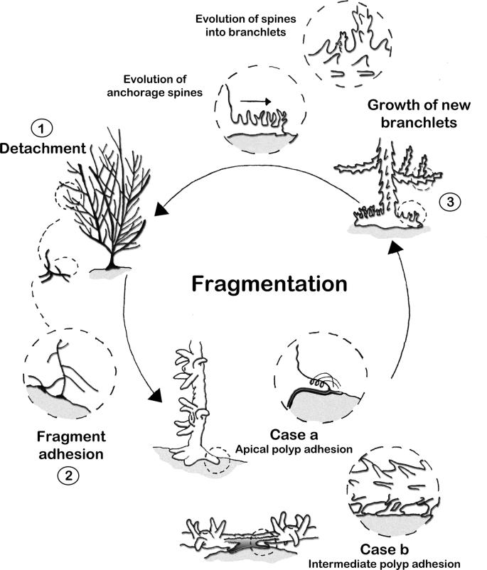
Withthenecessitytoconserveallcorals,variouspassiveandactiverestorationtechniques havebeenemployedglobally.Passivetechniquesincludeprotectiontoallownatural rejuvenation,whereasactiverestorationcomprisesimmediateinterventionthatintendsto acceleraterecovery.(TheNatureConservancy,2021).Passivemethodstakeprecedenceasan approach,however,cantypicallyonlyoccurwherecentralcontributorstosurvivalamid temperaturerisearepresent.Themainfactorsare;

● Geneticallypredisposedtosurvivewarmertemperatures

● Naturallyprotectedfromhotspellsduetocoldcurrents

● Abletoconstantlyremainwell-fedduetoplanktonpresence Reefslackinginthisnaturalprotectionoftenresultinmoredirebleachingevents,requiring activerestorationprocedurestobeimplemented.Withthescantknowledgeofbleaching susceptibility,scientistsmusttakeavarietyofapproachestofindaconservationmodelthat suitsmanycoralgenus.(Dance,2019).Dance(2019),aimedtointroduceenoughnewcorals toallowthereeftoreproduceindependently. Todoso,ocean-basednurserieswere

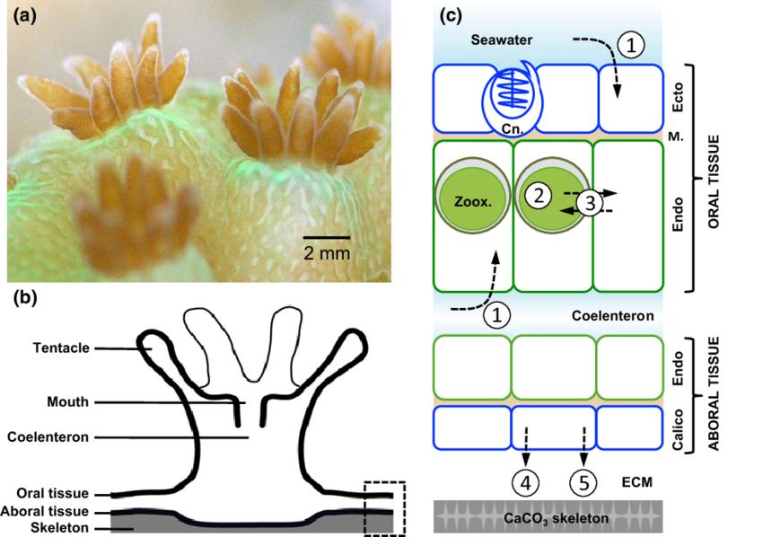Figure1a.CoralFragmentation Figure1.bAcroporapolypbranching

establishedintree-likestructuresandlefttogrow.Asampleofthegrowncoralwasthen testedintheenvironment,andifprovensuccessful,wasplantedontheseafloor.(figure2) Thismethodhasproventobeprosperous,however,thearticledoesnotmentiontheprocess toselectthecoralused,onlyspecificallyreferencingtheiruseofAcroporidcorals.Theother mostprominentapproachtocoralconservationshiftstheemphasisawayfromstudythecoral itself,andratherthechangestotheenvironmentinstead.DeCarloetal(2020)testedtherole ofnutrientsinmodulatingbleachingsusceptibility,revealingnutrientstressisequallyafactor ofbleaching(figure3).ThisworkwasconsistentwithsimilarstudiesconductedintheRed Seaandthusprovidedareliableperspective,assertingtheneedtoshiftscientificfocuses.

Inrecentyears,therehasbeenaninclinationtoconcentrateonthegeneticsofcoral,inwhich understandingthegeneticmechanismsthatunpinbleachingisconsideredfundamentalto conservation.(Bay,2020)Themajorimpedimentsinunderstandingcoralmolecularandcell biologyincludethedeficitofexperimentallycompliantmodelsandofgenetictechniquesthat assessproteinfunctionandgeneexpression.(Clevesetal,2020)However,abreakthrough study,Clevesetal,(2020)hasutilisedthemicroinjectionofCRISPR/Cas9intoanAcropora specie,tomutatetheHeatShockTranscriptionFactor1(HSF1).Todoso,twosgRNAswere createdtotargetexonsandcauseaframeshiftmutation,producinganon-functionalprotein. ItwasfoundthatcoralswiththeHSF1mutationhadreducedthermaltolerance,thus confirmingtheimportanceofthegene.Duetothevarietyofthetranscriptionfactor,however, themostvitalHSF1targetinstressreductionremainsunknown.Thisresearchhassincebeen republishedglobally,providingscopeforfurtherresearchworldwideregardingspecificHSF1 targetsandtheirexactroles.

Astheeffectsofclimatebecomemorepronounced,theneedtoconservecoralreefsbecomes increasinglyurgent.WhileresearchshowsthehistoricalsignificanceoftheAcroporaspecies, acceleratinganthropogenicpressureshaveinitiatedthecoral’sdecline.Resultingly,various passiveandactivemethodshavebeenimplementedtostopandreservethedevastation.From traditionallylabour-intensivesetups,nutrientregulationandgeneknockoutmethods,a varietyoftechniqueshavebeentested. Thereisprogressbutthequestion,however,remains astowhetheraspecificspeciesismorelikelytosurvivethanothers,andwhetherthe synthesisofnewtechniquesshouldadheretothis.

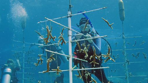
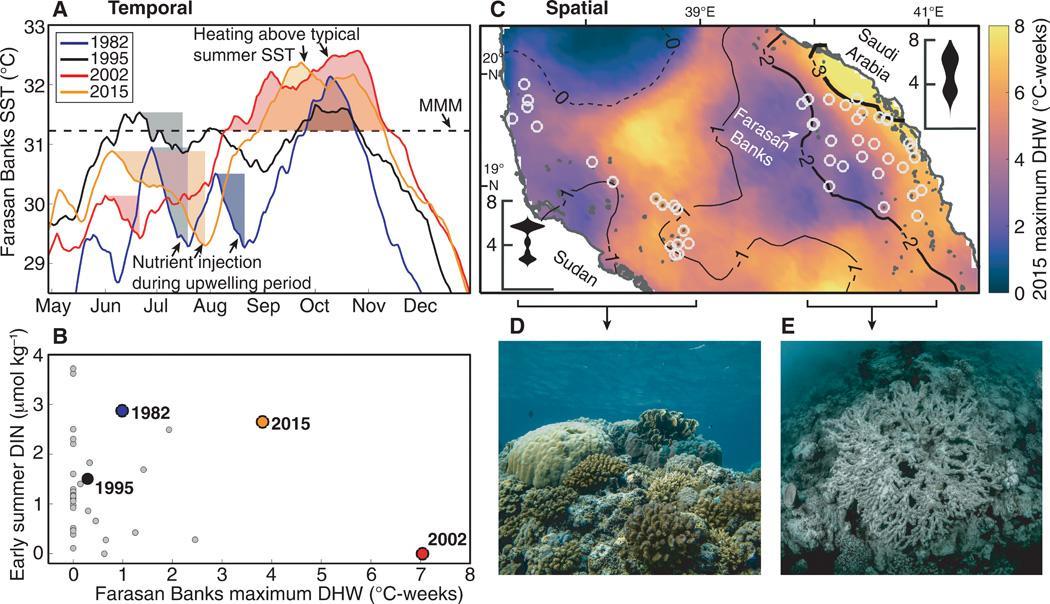Figure2;Ocean-basednurseryinCuraçaoislandFigure3; Coralbleachinginresponsetoofheat&nutrientstress

ScientificResearchQuestion:

HowdoestheuseofAcroporidCoralsaffecttheefficacyofreplantationprojects,as measuredthroughmeta-analysisofamultivariabledatabase?

ScientificHypothesis:

HA:ThereplantationstudiesthathaveusedAcroporaastheirprimarycoralwillproduce higherefficacyscoresthanthosethatdidnot,duetotheextensiveunderstandingand historicaldominanceofthecoral.

Methodology: Ethics Statement

ThisresearchwasconductedinconsultationwiththeHeadOfScienceatSantaSabina College,whichinvolvedreceivingethicalapproval.Throughthisprocess,riskswithinthe datacollectionstageswereanticipatedandhence,alleviated.Thesecondarydatawas obtainedthroughthepubliclyaccessible‘Coral RestorationDatabase 2020’aspublishedby theInternationalCoralReefInitiative(ICRI)(figure1/below).Allfollowingmeta-analysis wasconductedjudiciously,ensuringanaccuratereflectionofthegivendatawasrepresented.

Study Design

Duetothenatureofthisresearchproject,theinitialstepnecessitatedfindingrelevant secondarydata.Oncethiswasacquired,aformulawasderivedasametrictomeasurethe efficacyofeachrestorationproject. Figure 2 highlightstheprocessofethicallycreatingthe formulatoapply,inwhichrelevantcolumnswithinthedatabasewereselectedand manipulatedtoreducetheriskofinflatingthefinalscore.

Inclusion/exclusion Criteria

Toensurevalidresearchcurrency,allreefrestorationprojectsconductedbeforetheyear2000 wereexcludedfromthestudy.Further,anystudiesthatdidhaveavalueprovidedinoneof theeightcolumnsusedintheformulawereexcluded.

Data Collection

Theformulawasappliedtotheremaining133studies,eachproducingacomparablevalue forefficacy.TheuseofAcroporidcoralwasthenidentifiedastheindependentvariable,and thescoresweresubsequentlydividedintothosewithandthosewithout,asshowninfigure3. Studiesthatusedmorethan4species,includingAcropora,wereidentifiedseparatelyand discardedbeforefurtheranalysis.

Data Analysis

Themean,median,rangeandstandarddeviationofeachsetofdatawerecalculatedusing standardcalculations.(figure4a)AnF-testwasthenusedtodeterminewhetherthevariance betweenthetwodatasetsissignificantlydifferent.Thef-testresultisalwaysaboutthenull hypothesis,whereifthecalculatedp-valueisgreaterthanthealphavalue,thenull hypothesis cannotberejected(figure4b).Atwo-tailedt-testwasthenappliedtodeterminewhetherthe

nullhypothesis(thatstudiesusingAcroporidcoralswerenotmoreefficaciousthanthose without)couldberejected(figure4c).

Results

Figure 1 - Sample from the Coral Restoration Database Accessible through; https://docs.google.com/spreadsheets/d/1qLZV4crHMj26t96leX3rt_cFCR9QfjaXpbgChGohBxU/edit#gid=1206000473

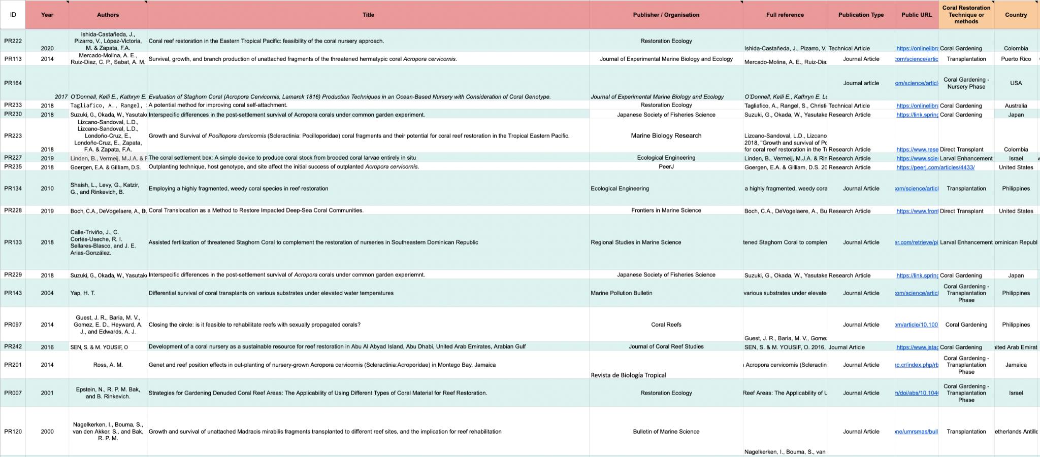
Figure 2a - Justification and process of creatinga formula to measure the efficacy.

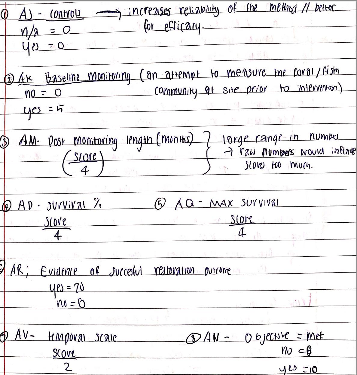
Columnsthatnaturallyprovided largervaluesweredividedtoreduce inflation,whereastherestwere simplyadded.

Incolumns,AJ,AKandAR,thedata waspresentedasyesorno’s, however,thesecolumnswerevitalin calculatingefficacy,soanumerical valuewasassignedtoeachword.

Figure 2b - Final Formula - using columns from coraldatabase

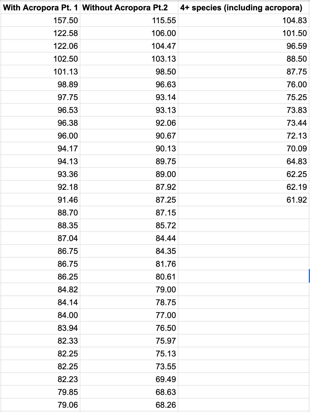
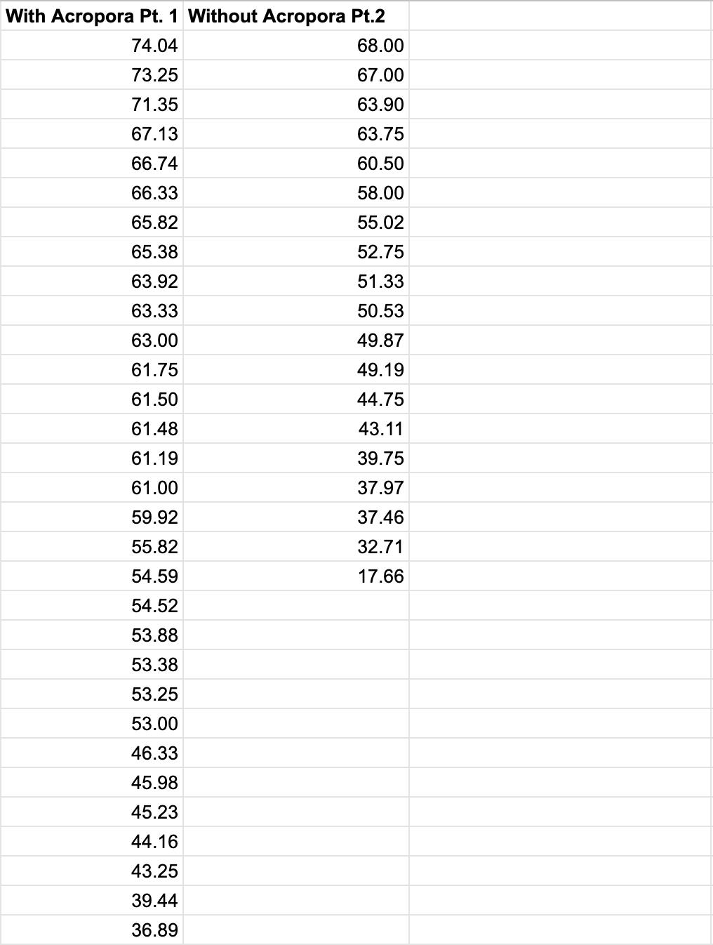
Figure 3 - Tables with efficacy metric sorted intostudies “With Acropora” and “Without Acropora” (table split across two images).

ThethirdcolumnwascreatedforstudiesthatmentionedAcropora,aswellasfourormore otherspecies.Thiscolumnwassubsequentlydisregardedinfurthercalculations,duetothe lackofspecificity.

Figure 4a - Means and standard deviations

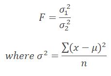
Lowerorderstatisticaltestswerecompletedonbothgroups,asdisplayedinthetable.

GroupA(withAcropora) GroupB(withoutAcropora)

Mean 75.91 72.54

Median 76.55 75.24

Range 120.61 97.33

StandardDeviation 22.06 21.69

Thegraphshowsthe meanandstandard deviationsofthe efficacyofeachgroup, using10%errorbars.

ThemeanofgroupAis higherthanthatof groupB,however,the standarddeviationand medianaresimilar.To determinewhetherthe differenceinoverall efficacyineachgroupis statisticallyanF-test wasapplied.

Figure 4b - F-test

● Usetodeterminewhetherthevarianceis statisticallysignificant

● Alwaysinreferencetothenullhypothesis;

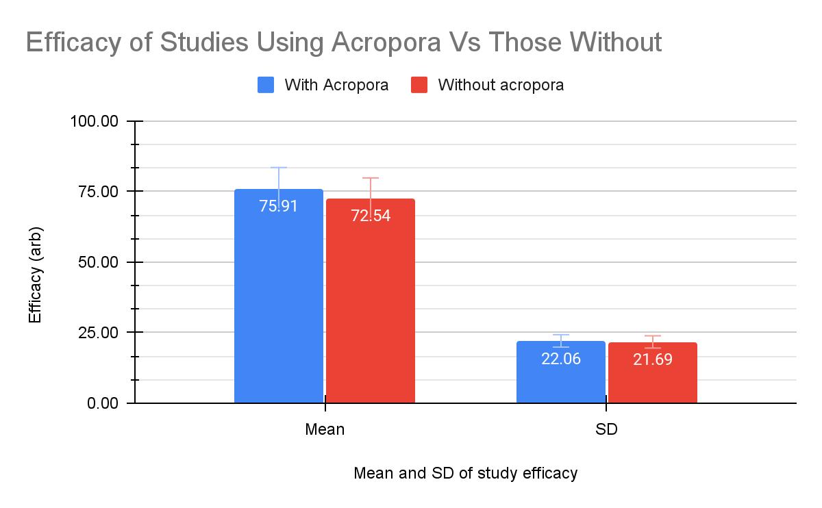
HO:TheuseofAcroporidcoralsdoesnotenhancethe effectivenessofreplantationstudiesandthusprojectsthat focusonthegenuswillnotproduceahigherefficacyscore.

● IfP> ��,thenullhypothesiscannotberejected

● FValue=Largersamplevariance/Smallersample variance

GroupA

GroupB

SampleMean 75.914 72.537

SampleSD 22.059 21.690

Populationsize 64 50

CalculatedP-Value 0.416

CriticalF-Value(��) 0.05

ThecalculatedP-value>CriticalFvalue,meaningthenullhypothesiscannotberejected. However,afurtherstatisticalanalysismustbeappliedtoensurethevalidityoftheseresults.

Figure 4c - Unpaired T-test

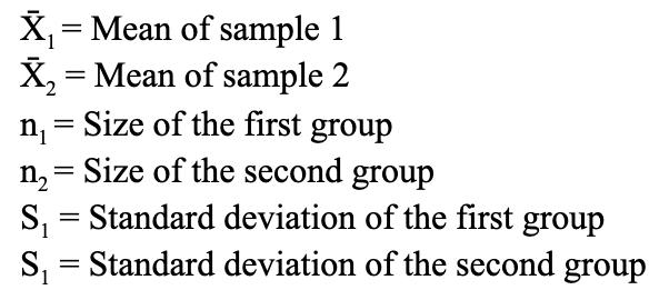
● Astatisticaltestofwhethertwosamplemeansare equal.

○ Thistestisappropriatewhenthe variancesofthetwopopulationsareequal

● Alwaysinreferencetothenullhypothesis

● IfT> ��,thenullhypothesisisrejected(=HA)

DegreesofFreedom 112

Critical(��)Value 1.980

T-value 0.817

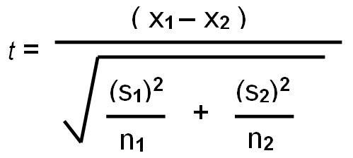
ThecalculatedTvalue<criticalvalue.Thereismorethana5%probabilitythatthe differenceinmeansisduetochance.Thenullhypothesisisaccepted.

Discussion:

ThisresearchpapertestedwhethertheuseofAcroporidCoralsinreplantationprojects alteredthestudy’soverallefficacy.Duetotheextensiveunderstandingofthecoralgenus,as wellasitshistoricaldominance (Pavid,2016),itwashypothesizedthatstudiesthatprimarily focusedonAcroporawouldhavehigherlevelsofpotency.Aftertheefficacywasmeasured, usinganarbitraryformula (figure2),itwasfoundthatstudiesthatusedAcropora(groupA) hadatopscoreof157.50,whereasthetopscoreofthosethatdidn't(groupb)was115.55. However,themeansofeachgrouphadamuchsmallerdifference,inwhichgroupA exhibitedameanof75.91,whereasgroupBproducedaslightlyloweraverageof72.54.

Accordingly,amorecomplexstatisticalanalysiswasrequiredandprovedthatthedifference inmeansnorvariancewasnotstatisticallysignificant (figure4),andthustheuseofAcropora doesnotenhancethepotency.

Statistical analysis

Todeterminewhetherthenullhypothesiscouldberejectedornot,higher-orderstatistical analyseswereappliedtothedata.Generally,anF-testisusedtodeterminewhetherthe variancebetweentwodatasetsissignificantlydifferent,andsubsequentlydecideswhichtype oft-testmaybeundertaken.AnF-testwasselectedasbothgroupsarehighlyvariable,thus necessitatingacomparisonofthevariationbetweendatasets.TheresultoftheF-testis alwaysinreferencetothenullhypothesis(HO),whereifthecalculatedp-valueislessthan thegivenαvalue,thenullhypothesismustberejected.Whendetermined,usingthemean, standarddeviationandrangeofeachgroup,thep-valueequalled0.415 (figure4),wherethe criticalαvaluewas0.05.Assuch,p-value>αvalue=HO couldnotberejected.Furthermore, theunpairedt-testisastatisticaltestofwhethertwosamplemeansareequal,inwhichthe twogroupsareindependent.AsthemeansofgroupAdidnotaffectthoseofgroupB,this testwasselectedtofurtherattesttoaconclusivefinding.

Ifthecalculatedt-value>givenαvalue,=HAthenullhypothesismustberejected.When solved,theT-valuewas0.817,whichwaslowerthanthepredeterminedcriticalvalueof 1.980, (figure4)whichfurtherassertedthatthenullhypothesiscouldnotberejected.Assuch, itwasproventhatthespecificuseofAcroporidcoralsdoesnotenhancetheefficacyofa replantationstudy.Thedata,however,islimitedduetothespecificityoftheindependent variable,asthereareonlytwogroupsavailableforfinalcomparison,meaningthatthereare noidentifiabletrendsbetweenstudies.Assuch,furtheranalysisintothetypesofstudyand locationwouldenhancetheoverallvalueofthispaper.

Accounting for the null hypothesis Despitelimitations,thefindingsofthisresearchareconclusivewithpeer-reviewedpapers,in thatthedeclineofAcroporaislargelyattributedtoincreasinganthropogenicpressuresandis, therefore,morevulnerableincurrentclimates (Sakaietal.,2019).Assuch,thenewfound knowledgethatAcoproadoesnotincreasestudysuccessisconsistentwiththerecognitionof itsrecentmortality.

WhilsttheAcroporagenushaspreviouslybeenidentifiedasthemostabundantcoral,there hassincebeenanotabledeclineincoralcoverageglobally,placing⅓ofallcoralatriskof extinction (Carpenteretal.2018).Scientistsareconsequentlyendeavouringtodiscovernew conservationmethodswhichsuitthemajorityofreefs,manyofwhicharelargelyAcropora species.AstudyreleasedinNovember2020showedthatHSF1hadavitalroleinAcroporid heattolerance,uncoveringamajorbreakthroughintocoralgenomics.Thisdiscovery subsequentlyinspiredtherationalethatstudiesusingthecoralwouldbemoreefficacious,as itdemonstratedacomplexunderstandingonagenomiclevel (Clevesetal.,2020).Thispaper, however,wouldnothaveinfluencedanyofthestudiesfoundintheCoralRestoration Database,astheywereallcompletedby2020&thuscouldnotyethaveappliedthis knowledgefortechniques.Hence,theresultsofthispapershowedthatthenullhypothesis

couldnotberejectedbutwithincreasinggenomicbreakthroughs,thismaychangeinfuture studies.

Validity, Reliability, Accuracy and Ethical Considerations

Thevalidityofanexperimentreferstothecontrolleduseofvariablestoaddresstheaim (internal)andwhetherthesucceedingconclusioncanexplainthephenomenon(external). Validitywashenceachievedastheexperimentonlyusedoneindependentvariable(theuseof Acropora),whichwaskeptclearlydefined.Thefollowingeffectoftheindependentwas measuredthroughthedependentvariable,beingtheefficacyscore.Thephenomenon demonstratedwasthattheuseofAcroporadidnothaveastatisticallysignificanteffectonthe efficacyofstudies.Theconclusionwasabletoexplainthisfinding,asmethodshavenotyet beenbetteradaptedtosuitthisspecificgenusnorhavetheyaccountedforitsvulnerability duetochangingtemperatureandpH.However,thevaliditycouldbeimprovedthroughthe useoftwocontrolstudies,whichkeptallvariableswithintheirexperimentaldesigntheexact samebutfortheuseofAcropora.

Reliabilityreferstothesizeofthedataandtherepeatswithconsistentresults.Duetothe natureoftheresearch,norepeatsweretrialled,hencelimitingthereliability.Thatbeingsaid, thefinaldatacontainedalargesamplesizeof112,beingreflectiveofmanypublishedand crediblereplantationstudiesconductedinthepast20years.

Theaccuracyoftheexperimentwassuppressedthroughthecreationofanarbitrarymetricfor efficacy,asitisnotcomparabletootherstudies.However,intheproductionoftheformula, skilfulchoicesweremadesoastoreducetheriskofinflation/deflationfromspecificcolumns (figure2).Asthiswasameta-analysis,alldatawasethicallyobtainedfromapublicly accessiblesite.Nevertheless,theresultsmaystillhavebeeninfluencedbybiaswhenselected foruseeg.allstudiespriorto2000wereculled.

Limitations and Areas for Future Research

Byobligation,variousmetricshavebeenusedfromthegivendatabasetocomparedifferent coralrestorationexperiments.However,factorssuchasthesurvivalratesmaynotbea suitabledeterminantofefficacy,duetotheincreasedriskofbias.Publisheddatahas inadequateincentivetoproduceunsuccessfulprojects,likelyduetogeneralconcernsofnot appeasingtheintendedaudience.Assuch,thereispresumablyageneralbiasfavouring survival.Survivorshipmayalsobeinflatedthankstoshorterexperimentaltimeframesor areasofnaturallyhighsurvival.Furthermore,anabsenceofuniformityinreportingsuccess limitstheabilitytocomparestudies,evenwithvaluesprovidedforeachmetric.Thedeficitof specificityindistinguishingfragmentsize,forexample,hindersfurtherabilitytoanalyse projectsanddeterminehowtofairlycomparethem.Anadditionallimitationofthisresearch paperisthelackofdetailexploredineachindividualstudy.Thoughtheindependentvariable wasidentifiedandhandledaccordingly,therewasnoacknowledgementofdifferencesinthe methodsbeyondjustthecoralused.Assuchitisrecommendedforfuturestudiestorecognise thedifferencesbetweeneachstudyandidentifyanotherfactortobeconsideredaspartofthe

independentvariable.Genomicsendeavoursarealsocrucialtosavingcoral,wherebythe morecomplexknowledgemustbeappliedtorestorationtechniques.

Conclusion

ThisstudyaimedtofindwhethertheuseofAcroporidcoralsenhancedtheefficacyofthe replantationprojects.Ameta-analysisofthe‘CoralRestoration Database’ wasconducted,in whichanarbitrarymetrictomeasuretheefficacyofstudieswasapplied.Thefollowing scoresweredividedintotwogroups;studiesthatfocusedonAcroporaandthosethatdidn’t andwerecompared.Thoughtherewasaslightdifferenceinmeans,statisticalanalysisproved thisdifferencetobeinsignificant.Assuch,thenullhypothesiscouldnotberejected,meaning thattheuseofAcroporainreplantationprojectsdoesnotenhancetheefficacyofthestudy. Thisislikelyduetothevulnerabilityofthecoralgenusinenvironmentswithincreased temperature,pHornutrientdensity,asexasperatedbyclimatechange.Furthermore, breakthroughunderstandingsofAcroporahavenotyetbeenimplementedintorestoration techniques.Thispaper,therefore,assertstheneedforfurtherresearchintothefactorsthat enhancereplantationmethodstoprovidecoralreefswithachanceforsurvival.

Bauer,A.(2021). Importance of Coral Reefs - Biodiscoveryand the Great Barrier ReefQueensland Museum.Qld.gov.au;QueenslandMuseum. https://www.qm.qld.gov.au/microsites/biodiscovery/05human-impact/importance-of-coral-ree fs.html

Cleves,P.A.,,Bradford,J.,&Bay,L.K.(2020). Reduced thermal tolerance in a coral carrying CRISPR-induced mutations in the gene fora heat-shock transcription factor. NationalAcademyofSciences, https://doi.org/10.1073/pnas.1920779117

Cramer,K.L.,Jackson,J.B.C.,Donovan,M.K.,Greenstein,B.J.,Korpanty,C.A.,Cook, G.M.,&Pandolfi,J.M.(2020). Widespread loss ofCaribbean acroporid corals was underway before coral bleaching and disease outbreaks. ScienceAdvances,6(17), https://doi.org/10.1126/sciadv.aax9395

Dance,A.(2019). These corals could survive climatechange -- and help save the world's reefs. NaturePublishingGroup. https://link.gale.com/apps/doc/A650920221/AONE?u=61ssc&sid=bookmark-AONE&xid=d 00d5864

DeCarlo,T.M.,Hammerman,N.M.,Pandolfi,J.M.,Monroe,A.A.,&Berumen,M.L. (2020). Nutrient-supplying ocean currents modulatecoral bleaching susceptibility. Science Advances https://doi.org/10.1126/sciadv.abc5493

Hoegh-Guldberg,O.(1999). Climate change, coral bleachingand the future of the world’s coral reefs. MarineandFreshwaterResearch.https://doi.org/10.1071/mf99078

InternationalUnionforConservationofNature.(2017). Coral reefs and climate change IUCN.https://www.iucn.org/resources/issues-briefs/coral-reefs-and-climate-change

Pavid,K(2016). World's most important coral speciesin major decline. NaturalHistory Museum. https://www.nhm.ac.uk/discover/news/2016/april/worlds-most-important-coral-in-major-decli ne.html

Sakai,K.,Singh,T.,&Iguchi,A.(2019). Bleachingand post-bleaching mortality of Acropora corals on a heat-susceptible reef in 2016. PeerJ,7,e8138. https://doi.org/10.7717/peerj.8138

SECOREInternational | Why coral reefs need our help.(2015).Secore.org. http://www.secore.org/site/corals/detail/why-coral-reefs-need-our-help.23.html

USDepartmentofCommerce,NationalOceanicandAtmosphericAdministration.(2021). What is coral bleaching? Noaa.gov.https://oceanservice.noaa.gov/facts/coral_bleach.html

VanOppen,M.J.H.,&Oakeshott,J.G.(2020). A breakthrough in understanding the molecular basis of coral heat tolerance. ProceedingsoftheNationalAcademyofSciences. https://doi.org/10.1073/pnas.2020201117

Investigating how the Height (from 0.0000 5.0000 ± 0.0005 m) from which Water falls impacts the amount of Hydropower (W) produced.

1. Context:

Renewable energy sources such as hydropower are more sustainable, increasingly available, and important for addressing Climate Change. Coal power stations “can only extract 25% of the energy” from their “fuel source” while “hydropower stations… achieve over 90% efficiency,” (Clean Energy Council, 2012). However, “coal and gas… still represent close to 60% of global electricity supply,” (IEA, 2020). In 2019, hydropower provided 16% of the world's electricity and produced 5 7% of Australia’s supply for decades, (Australian Government, 2021). Despite increasing use of renewable energy, they remain the minority while society remains dependent on non renewable energy sources that contribute to Climate Change. Consequently, as renewable energy is becoming increasingly necessary globally to reduce greenhouse gas emissions that contribute to Climate Change, this investigation explores the renewable energy source of hydropower which connects to Topic 8.

2. Research Question:

How does the height (from 0.0000 5.0000 ± 0.0005 m) water falls from impact the power (W) produced in a turbine powered electricity generator?

3. Aim: To investigate how hydropower (W) produced by turbine generators changes with the height water falls (from 0.0000-5.0000 ± 0.0005 m)

4. Background Research and Justification of Hypothesis:

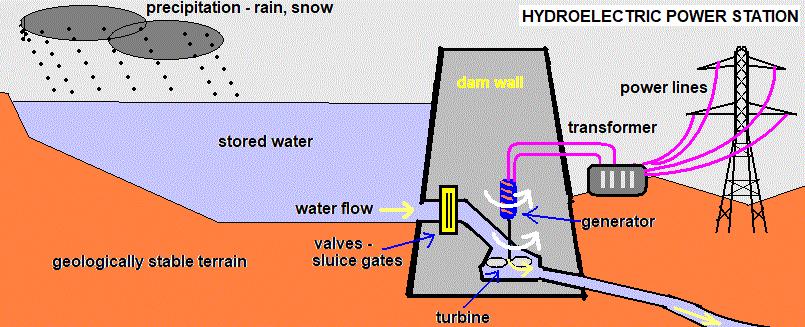
4.1 Primary Energy (Renewable & Non-Renewable Energy Sources) & Secondary Energy. There are two types of primary energy found in nature that have not been processed in any way, being either renewable or non renewable energy. Non renewable sources are “natural resources,” (Energy Education, 2020b) extracted from nature such as fossil fuels (i.e. oil, natural gas and coal). These fuels are not reusable and are finite, being depleted faster than they can be extracted. Future projections predict that oil availability will end by 2052, gas by 2060, and coal by 2090, (MAHB Admin, 2019). While “energy rich and relatively cheap to process,” (National Geographic Society, 2019), non renewables pollute and contribute greenhouse gases to the atmosphere, thus contributing to climate change. Conversely, renewable sources are natural processes from which energy can be extracted and transformed in a useful way. Relying on Earth's systems rather than Earth’s resources, they replenish their energy supply, rendering them environmentally sustainable. Examples include solar radiation from the Sun, or water falling from great heights from which solar and hydropower can be harnessed respectively.

Secondary energy is produced when primary energy is transformed into other forms of energy such as electricity or kinetic energy, that are easier and more convenient to use, transport, and/or store.

4.2 Hydropower & Hydroelectric Power Plants:

Hydropower is a renewable energy source derived from moving masses of water, infinite in supply because the water cycle is a consistently replenishing system. The kinetic energy of flowing water is converted into mechanical and electrical energy. It can store large amounts of energy and quickly produce power. However, it is dependent on location, requires drastic changes to the environment (eg; flooding of areas for dams), and initial costs as a result are high.

Hydroelectric power plants are generally turbine driven by water flow from a higher point. It requires an upper and lower reservoir of water. Energy can be stored as gravitational potential energy in the upper reservoir. Sluice gates or valves control the water flow and thus the rate of electricity generation. When water from the upper reservoir passes through the turbine, the pressure on the turbine’s blades causes the shaft to rotate.

Figure 1: Hydroelectric Power Station, (Brown, 2020).

The generator connected to the turbine then converts the motion, or kinetic energy, into electrical energy that can be transferred to power lines for people’s use. Though hydroelectric power plants typically only work in the one direction, a pumped storage system can reverse the direction of water flow to refill the upper reservoirs, (Brown, 2020)

4.3 Energy Store Changes: Gravitational Potential Energy ⇒ Kinetic energy ⇒ Electrical energy. Table 1: Energy Store Changes in hydroelectric power plants by stage, (Brown, 2020).

Stage Energy Store Mechanical Change

1 Gravitational Potential Energy stored in water from the upper reservoir 2 ⇒ Kinetic Energy of flowing water 3 ⇒ Kinetic Energy of the turbine rotation and generator rotation of a coil in a magnetic field 4 ⇒ Electrical Energy the generator outputs (from the rotation of the coil that produces an emf).

4.4 The Turbine:

The process’ efficiency depends on the turbine. In the investigation, Seeed Studio’s Micro Water Turbine (DC 5V) is used. Like in a hydroelectric plant, the pressure of flowing water rotates the turbine within the small device. Connected to the motor, it will rotate as well, generating electricity. The wires extending from the device can be connected to a circuit to measure voltage and current.

Table 2: Features and specifics of the turbine, (Seeed Studio, 2021 and Core Electronics, 2021b).

Feature Name Feature Feature Name Feature Maximum Output Voltage (V) 5.0 ± 0.3 Axial Clearance Approximately 0.2 1.0mm Maximum Output Current (mA) 150.0 Start Water Pressure 0.05 Mpa Resistance (Ω) 10.5 ± 0.5 Flow range (dm3.min 1) 3.5 20 Maximum Working Pressure 1.2 MPa Mechanical Noise ≤ 55dB Outlet Closed Highest Pressure Resistance 0.6 MPa Working Temperature Range 0 80 ° C

4.5 Variables affecting the production of Hydropower:

Table 3: The principle behind determining hydropower (used in Table 13, Appendix 1 2)

A mass of water (m) is falling down a vertical height (h). The potential energy, or work that can be harnessed is mgh, where g represents gravity. Thus…

Potential energy = work = kinetic energy = mgh

Power (P) then equals work done over time. P = �������� �������� = ����ℎ ��

Figure 2: Water falling from a vertical height h has its potential energy converted into kinetic energy, which can be used to drive turbines, (Tsokos, 2014).

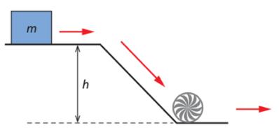
• P = Power (W).

• m = mass (kg).

• h = height (m).

• g = gravity = 9.81 m.s 2 .

The mass (m) then equals the product of the density of water (ρ) and the volume it occupies (∆V). P = ����ℎ �� = ��∆����ℎ ��

• m = mass = ρ∆V (kg). • ρ = the density of water = 1000 kg.m 3 . • ∆V = the volume it occupies (m3s 1)

The Quantity (Q), known as the flow rate, is the volume that passes through over time. Thus… P = ��∆����ℎ �� = ������ℎ

• ρ = the density of water = 1000 kg.m 3 . • ∆V = the volume it occupies (m3)

• Q = quantity = flow rate = ∆�� �� (m3.s 1).

In terms of energy, Power is also known to equal voltage by current. Thus the equation… P = VI ∴ VI = ������ℎ

• V = Voltage (V).

• I = Current (A).

4.6 Modelling Hydroelectric Power Plants: An Isolated Representation of Reality.

The investigation will attempt to imitate hydroelectric power plants with water falling vertically from the upper to lower reservoir, on a smaller scale using pipes and a turbine. A carton (Table 6 7) attached to the top of the pipe(s) acts as the upper reservoir, whilst water from a garden hose will be poured into the carton and piped through in a constant stream. The pressure from garden hoses on average is 1.37 2.41 MPa, (Williams, 2017), and exceeds the turbine’s maximum working pressure. By pouring the water through varying heights of the pipe (from 0.0000 5.0000 ± 0.0005 m) and measuring the voltage and current output of the turbine, the impact of the height on hydropower production can be determined experimentally (P = VI). A theoretical value can be ascertained for comparison using the equation P = ρQgh, wherein only the flow rate is subject to change and will be determined in the experiment.

5. Hypothesis:

Considering the equation VI = ρQgh (Table 3), voltage (V) and current (A) have a directly proportional relationship with the height (m) water falls from. Thus, as the height increases, so too should the voltage and current from the turbine generator and as such, the power (W)

6. Variables:

Table 4: Independent, dependent, and controlled variables and method of measurement or control. Type

Variable Method of Measurement or Control

Independent

Dependent

The height (± 0.0005 m) from which water falls from through a pipe before reaching the turbine. Six pipe heights: 0.0000 5.0000m tall. The power at 0.0000 m high will be subtracted from the others.

Ensure height of pipe is measured from the same point, using a ruler (to the nearest mm) to improve validity and reliability of method. Subtracting the power from 0.0000m high will account for possible zero errors (systematic), as hypothetically there would be no stored energy to be converted into power.

The Power (W) produced from the turbine generator. Use a correctly calibrated multimeter with a minimum of 2 decimal places to discern a digital reading of voltage and current with small uncertainty for precision and reliability.

Materials/equipment used.

Controlled

Use the same equipment and materials detailed in Table 6 for each trial in the method for validity.

Ensure different heights are equal increments apart for continuous data with a small uncertainty for precision. The density (ρ, kg.m 3) of the liquid passing through the turbine. The density of water = 1000 kg.m 3 .

Intervals from which height of pipe is measured (1.0000 ± 0.0005 m intervals).

Ensure the same liquid, from the same source, is used to avoid adversely affecting the validity of theoretical data Perform experiment at same location where temperature remains relatively constant (around 26°C), to not affect water density. The location/conditions (ie; temperature).

The proportion by which the flow rate (m3.s 1) changes.

Flow rate is influenced by the hose pressure and height water falls from. Ensure the hose’s tap turned the same proportion for all trials (a 3/4 turn). Using the same hose, the proportion flow rate changes should remain consistent with height. Hose Pressure (MPa). On average, 1.37 2.41 MPa, (Williams, 2017).

Acceleration due to gravity (g) = 9.81 m.s 1 , considering P = ������ℎ

Pipe diameter (mm). All pipes used will be 25 mm in diameter.

7. Risk Assessment:

Conduct the experiment in the same place.

Ensure the pipe is the same width so that only the length changes.

Table 5: Safety, environmental and ethical considerations

Hazard Risk Method to Control Risk

Slipping hazard.

Spilt water can pose a risk for people walking by, causing minor or severe injury through slipping or falling.

Handle all liquids outside (in a garden) to minimise the potential for water to go onto the floor or hard surfaces in a greater area.

Keep all electronics and the circuit as far from water as possible. If water is spilt, dry surface with towel Water spray. Water spray coming into contact with one’s eyes, causing slight irritation.

Water near electronics. Water coming in contact with electronics poses danger of electrocution.

Wear safety glasses and lab coat to protect oneself and one’s eyes from possible water spray.

Wastage of water. Wasting unnecessary amounts of fresh water would have a negative environmental impact.

Use water from a hose outside and collect water in a bucket to be used to water plants in the gardens so no water is wasted. As flow rate will be measured in a 1dm3 measuring cylinder, secure it to base of bucket so any spillage beyond 1dm3 can be caught. Cutting of pipes. Potential for serious injury of cutting oneself, particularly one’s hands. Cut the pipes with supervisor guidance and ensure no distractions while using the cutting equipment.

8. Equipment:

Table 6: Quantity (Qty), Brand and Uncertainty of Equipment.

Quantity Equipment Brand Uncertainty 1 Micro Water Turbine: Hydroelectric Generator 5V Seeed Studio ± 0.3 V 2 3.00 m tall PVC Pipes (25mm in diameter) Holmon ± 0.0005 m 1 Digital Multimeter (Cat: QM 1500) Jaycar ± 0.01 V 1 Milliammeter Scale: 50 mA PeakTech ± 0.5 mA Scale: 500 mA ± 5 mA 1 1000 cm3 Measuring Cylinder. Polylab ± 5 cm3 1 Measuring Tape Stanley ± 0.0005 m 1 Stopwatch Fastime ± 0.01 s 1 Packet of Blu Tack Bostik N/A 1 Duct Tape (48mm by 54.8 m) 3M N/A 5 Wires Haines Educational N/A 4 Alligator Clips Haines Educational N/A 2 Metal Bar from Retort Stand Haines Educational N/A 1 Hose connected to a tap outside Pope N/A 1 Diffused LED (5mm PTH) Sparkfun N/A 1 Hacksaw Stanley N/A 1 Clamp Trojan N/A 1 4 dm3 Distilled Water Carton Glendale Packaging N/A 1 Scissors Studymate N/A 1 Male Thread PVC Pipe Fitting Adapter Uxcell N/A 1 Bucket House & Home N/A 1 2B Pencil Staedtler N/A 1 Protective: Safety Glasses, Gloves and Lab Coat N/A N/A

9. Diagrams:

Table 7: Labelled Images of the Experiment (Method). Method Part 1 Method Part 2 Carton & Turbine Connector of Blu Tack surrounded by Duct Tape (for the 0.0000 ± 0.0005 m Pipe)

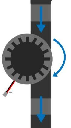
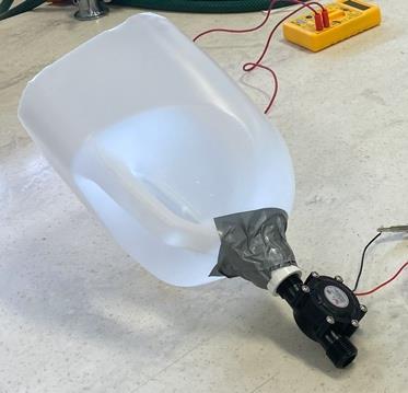
Micro Water Turbine (5V) (Seeed Studio, 2021 and Core Electronics, 2021b)

Circuit Diagram (Terminal/battery represents the 5V Micro Water Turbine)

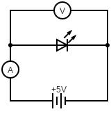
Method Part 2 Method Part 3

Blu Tack surrounded by Duct Tape

Connector between 2 Pipes with support metal bars

1.0000 3.0000 ± 0.0005 m Pipes

4.0000 5.0000 ± 0.0005 m Pipes

10. Method:

Part 1: Setting Up the Equipment for 0.0000m, 1.0000m, 2.0000m, and 3.0000m tall Pipes.

1. Cut the distilled water carton in half and discard the base.

2. Mark along the edge of one 3.0000m pipe at 1.0000m high using a pencil and measuring tape.

3. Secure the pipe with a clamp to ensure it does not move whilst cutting the pipe.

4. Cut the pipe along the marking made using a hacksaw.

5. Remove the now 1.0000m and 2.0000m high pipe from the clamp.

6. Place the end of the turbine generator against one end of the 1.0000m pipe.

7. Place Blu Tack all along the edge connecting the turbine generator with the 1.0000m pipe. This should also help prevent water from leaking in the gap.

8. Secure the turbine generator and Blu Tack to the bottom of the 1.0000m high pipe with duct tape, going around the pipe at least 4 times. This should also help prevent water leaking in the gap.

9. Place the lid opening of the water carton against the top end of the 1.0000m high pipe and secure using Blue Tack and duct tape to help prevent water from leaking.

10. Complete Part 3.

11. Repeat Steps 6 10 for the 2.0000m and then 3.0000m pipe lengths.

12. Repeat Steps 6 10 for the 0.0000m pipe length, attaching the water carton and turbine together directly using Blue Tack and duct tape to help prevent water from leaking.

Part 2: Setting Up the Equipment for 4.0000m and 5.0000m tall Pipes.

1. Connect a 1.00m pipe to 3.0000m pipe as previously to form a 4.0000m pipe.

2. Duct tape two metal bars from the retort stands on either side of where the two poles joined to improve the rigidity of the structure.

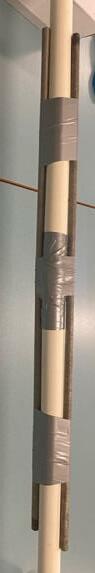
3. Connect a 2.0000m pipe to 3.0000m pipe as previously to form a 5.0000m pipe.

4. Repeat steps 6-10 from Part 1 with each pipe length.

Part 3: Obtaining Results

1. Set up equipment as per diagram (see Table 7) and described in Part 1 using the 1.0000m tall pipe.

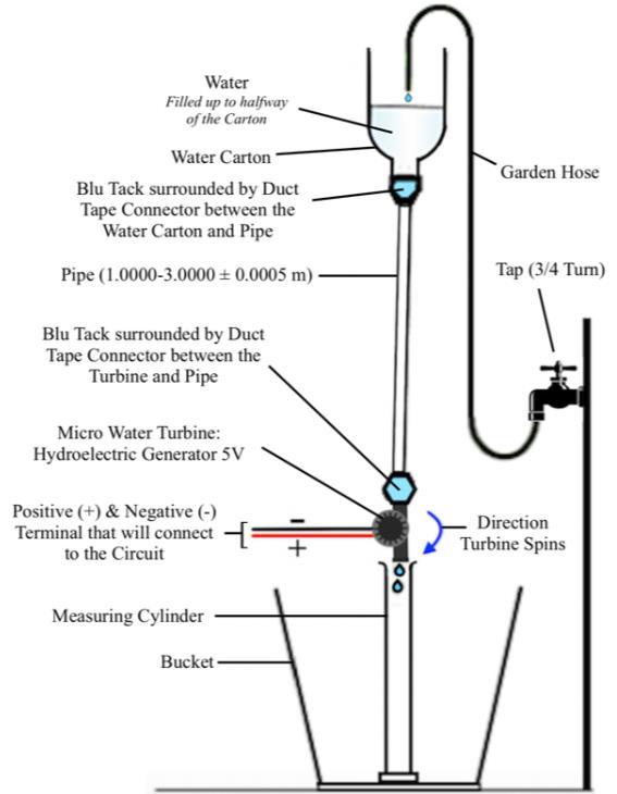
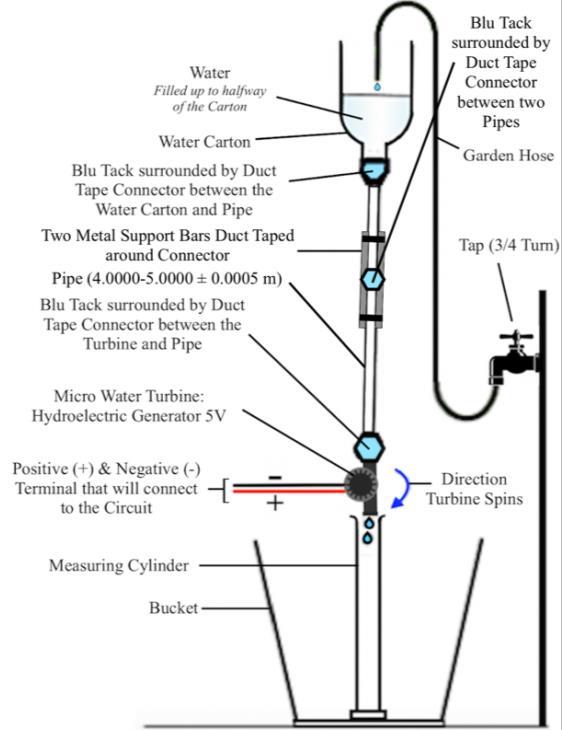
2. Attach a 1000 cm3 measuring cylinder to the base of a bucket.

3. Hold the pipe over the measuring cylinder.

4. Block the turbine’s opening at the base of the pipe.

5. Turn on the hose (3/4 turn) and wait until the water carton half is around half full.

6. Unblock the turbine’s opening to allow water to begin flowing into the pipe.

7. Record the time taken for 1dm3 of water to be filled using the measuring cylinder and stopwatch.

8. Record the voltage and current using the Multimeter and Milliammeter, respectively.

9. Turn off the hose.

10. Empty the measuring cylinder and bucket of water into the garden.

11. Repeat steps 1 10 four more times.

12. Repeat steps 1 11 for each other pipe length.

13. Clean up the workstation.

11. Quantitative Results:

Halfway through collecting data, the current exceeded the 50mA scale. The 500mA scale had to be used to measure current at 4.0000 5.0000m heights, seen in separate tables with different uncertainties to maintain precision in the preceding values taken with the 50mA scale (0.0000 3.0000m heights)

Table 8: Raw data for the Current (±0.5 mA), Voltage (± 0.01 V) and the Time to Fill 1 dm3 (± 0.01 s) when water falls from a Pipe of Heights (± 0.0005 m) 1.0000m, 2.0000m and 3.0000m tall. Height (± 0.0005 m) Trial Current (± 0.5 mA) Voltage (± 0.01 V) Time to Fill 1 dm3 (± 0.01 s)

0.0000 1 0.0 0.00 35.40 2 0.0 0.00 35.51 3 0.0 0.00 35.45 4 0.0 0.00 35.35 5 0.0 0.00 35.34

1.0000 1 11.0 2.00 15.14 2 10.0 2.00 14.86 3 11.0 2.00 15.09 4 11.0 2.00 15.02 5 10.0 2.00 14.94 2.0000 1 28.0 2.08 10.55 2 28.0 2.08 10.60 3 28.0 2.07 10.50 4 27.5 2.08 10.36 5 28.5 2.07 10.59 3.0000 1 38.0 2.13 8.50 2 39.0 2.12 8.66 3 38.5 2.09 8.62 4 38.0 2.10 8.55 5 38.0 2.10 8.58

Table 9: Raw data for the Current (± 5 mA), Voltage (± 0.01 V) and the Time to Fill 1 dm3 (± 0.01 s) when water falls from a Pole of Heights (± 0.0005 m) 4.0000m and 5.0000m tall.

Height (± 0.0005 m) Trial Current (± 5 mA) Voltage (± 0.01 V) Time to Fill 1 dm3 (± 0.01 s) 4.0000 1 50 2.12 7.36 2 55 2.13 7.53 3 50 2.11 7.46 4 50 2.12 7.39 5 55 2.12 7.44 5.0000 1 60 2.14 5.42 2 60 2.14 5.40 3 60 2.14 5.41 4 60 2.14 5.45 5 60 2.14 5.42

12. Qualitative Results:

Table 10: Qualitative data observed during the experiment. Process Observation

Water initially filling the carton. After the hose was turned on, the base of the turbine was blocked to allow the carton at the top to fill up to halfway. When turbine was unblocked, for the carton to remain consistently filled to halfway, the tap had to be adjusted consistently from a 3/4 turn.

Water falling through the pipe and exiting turbine

13. Data Processing:

The water flow when it exited the turbine at the base of the pipe was laminar (smooth and regular). As the height increased, the same volume of water filled the measuring cylinder in a shorter time and the flow seemed stronger.

Table 11: The Average; Current (± 0.5 mA & ± 0.0005 A), Voltage (± 0.01 V) and Time to Fill 1dm3 (± 0.01 s) when water falls from heights 0.0000 3.0000m ± 0.0005 m tall, (Appendix 1 2).

Height (± 0.0005 m) Average Current (± 0.5 mA) Current (± 0.0005 A) Voltage (± 0.01 V) Time to Fill 1dm3 (± 0.01 s)

0.0000 0.0 0.0000 0.00 35.41

1.0000 10.6 0.0106 2.00 15.01 2.0000 28.0 0.0280 2.08 10.52 3.0000 38.3 0.0383 2.11 8.58

Table 12: The Average; Current (± 5 mA & ± 0.005 A), Voltage (± 0.01 V) and the Time to Fill 1dm3 (± 0.01 s) when water falls from heights 4.0000 5.0000m ± 0.0005m tall, (Appendix 1 2).

Height (± 0.0005 m)

Average Current (± 5 mA) Current (± 0.005 A) Voltage (± 0.01 V) Time to Fill 1dm3 (± 0.01 s) 4.0000 52 0.052 2.12 7.44 5.0000 60 0.060 2.14 5.42

Table 13: The Experimental Power (W), Average Flow Rate, Q (m3.s 1) & Theoretical Power (W), for each height (0.0000 5.0000 ± 0.0005 m), (Table 3, Appendix 1 2). Height (± 0.0005 m) Experimental Power, P (W) Average Flow Rate, Q (m3.s 1) Theoretical Power, P (W)

0.0000 0.0000 ± 0.0000 2.82 x 10 5 ± 1.49 x 10 7 0.0000 ± 0.0000 1.0000 0.0212 ± 0.0011 6.66 x 10 5 ± 3.77 x 10 7 0.6536 ± 0.0040 2.0000 0.0581 ± 0.0013 9.51 x 10 5 ± 5.66 x 10 7 1.8650 ± 0.0116 3.0000 0.0807 ± 0.0014 11.65 x 10 5 ± 7.18 x 10 7 3.4293 ± 0.0217 4.0000 0.110 ± 0.011 13.45 x 10 5 ± 8.53 x 10 7 5.277 ± 0.034 5.0000 0.128 ± 0.011 18.45 x 10 5 ± 12.62 x 10 7 9.050 ± 0.063

Table 14: Percentage error for each height (0.0000 5.0000 ± 0.0005 m), (Appendix 3). Height (± 0.0005 m) 0.0000 1.0000 2.0000 3.0000 4.0000 5.0000 Percentage Error (%) 0.0000 96.7562 96.8832 97.6457 97.911 98.581

14.Graphs:

Table 15: The Relationship between the Height (0.0000 5.0000 ± 0.0005m) from which water falls and the Theoretical (W) and Experimental Power (W) produced.

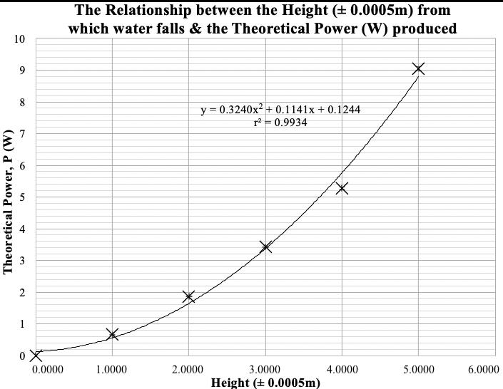
Graph 1: Experimental Power, P (W) Graph 2: Theoretical Power, P (W)

15.Analysis:

15.1 Describing Trends:

The line of best fit in Graph 1 (LOBF 1) indicates that there is a linear directly proportional relationship between the height from which the water falls through the pipes (0.0000 5.0000 ± 0.0005m) and the power produced (W). While not all values pass within the error bars of the graph (from 1.0000 2.0000 ± 0.0005m heights), the same number of points are above and below the line and uncertainties are small, indicating high precision (± 0.0005m for height and ± 0.0000 0.011 W for experimental power). This is reinforced by the high r2 value (r2 = 0.9928) and correlation constant (r = 0.9964), indicating a strong correlation. Thus, the LOBF 1 in Graph 1 supports the hypothesis, power increases as height increases.

Similarly in Graph 2 detailing the expected theoretical power (W) produced, the line of best fit (LOBF 2)has a high r2 value (r2 = 0.9934), indicating a strong correlation. While not all values pass within the error bars of the graph (at 0.0000m, 2.0000m, 4.0000m and 5.0000m heights), the same number of points are above and below the line and the uncertainties are small, indicating high precision (± 0.0005 m for height and the range ± 0.0000 0.063 W for theoretical power). Whilst the power is still suggested to increase as the height increases, the LOBF 2 is a curved line, indicating a non linear relationship between the height and power produced, slightly deviating from the predicted directly proportional relationship, considering the equation VI = ρQgh (Table 3).

Error

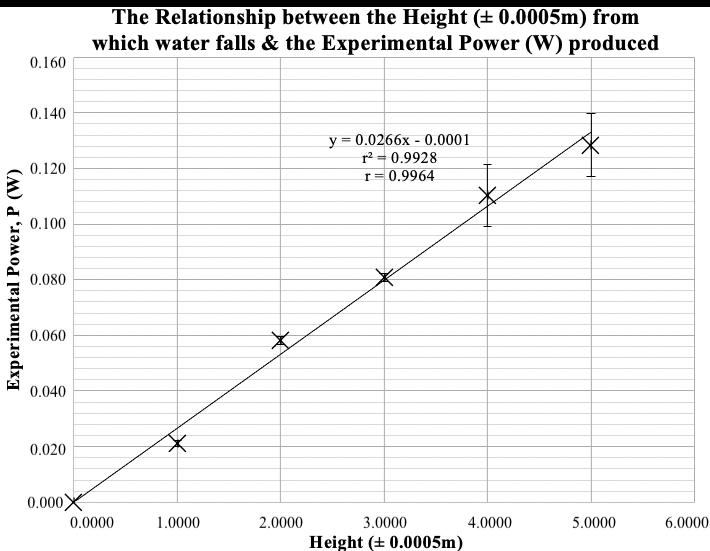
The varying scales on the y axis required to present the data in Graphs 1 and 2 alongside the differing shapes of LOBF 1 and LOBF 2 indicate low accuracy when comparing the expected theoretical and experimental power produced. This is reinforced by the high percentage error (Table 14) for heights 1.0000 5.0000 ± 0.0005 m high, (the 0.0000 m height the exception), and the theoretical values (m = 0.3240) greater rate of increase than the experimental values (m = 0.0266).

15.2 Explaining Trends:

In Graph 1, the larger error bars for 4.0000 5.0000 ± 0.0005m heights reflect the change of scale required to measure the current (from 50mA to 500mA) for the experimental power since it exceeded the limit using the smaller scale. The different shapes of LOBF 1 and LOBF 2 can be attributed to the varying scales of power produced, (0.0000 0.1600 W in Graph 1 and 0.0000 10.0000 W in Graph 2). Due to the larger scale in Graph 2, what initially appears as a linear relationship in Graph 1 could potentially imitate the curve of Graph 2 as more power is produced. The difference was perhaps also because the flow rate (Q) did not change proportionally as the height increased, (Table 13).

The large percentage error is perhaps indicative of the efficiency of the turbine and the effectiveness of the height. The calculation of theoretical power assumed all the energy produced by the falling water

converted into electrical power (Table 1 and Table 3), and that the turbine and generator were both 100% efficient. In reality, efficiency is “always less than 100%,” (Open University, 2020). With proper infrastructure, efficiency is around 80 90%, (Blakers, Lu, & Stocks, 2020). Considering this is a model using pipes, duct tape, Blu Tack and a 5V turbine generator, the system would likely be far less efficient. As water passes through the pipe and turbine generator, at each stage depicted in Table 1 there will be a loss of energy to the water, reservoir walls (the carton and pipe walls), turbine, and generator due to sound, heat and friction (Open University, 2020), since “water is doing work against the surface of pipes and turbine blades,” (Brown, 2020) and the turbine has mechanical noise ≤ 55dB (Table 2). The turbine itself has a resistance of 10.5 ± 0.5 Ω which would restrict the current (A) that could pass through the circuit, limiting the experimental power measured.

Unlike a real hydroelectric power plant, not all water used to calculate flow rate nor experimental power dropped from the expected height, for both the carton and pipe were full before the investigation began. Some dropped from anywhere between 0.0000m and the total height. The 0.0000 m height was the exception with no percentage error considering it did not produce any power. At 0.0000 m high, there would be no potential energy in water to convert to kinetic and then electrical energy (Table 1). Experimentally, this is reinforced by the flow rate at 0.0000 m high (2.82 x 10 5 ± 1.49 x 10 7 m3.s 1), which was not within the turbine generator’s flow range required (3.5 20 dm3.min 1) to produce power.

The large discrepancy between the theoretical and experimental power produced is also because the voltage (V) measured was limited to the LED attached in parallel to the multimeter [with voltage range 2.0 2.4 V, (Core Electronics, 2021a)]. All measured values for voltage (V) fell within the range, and were perhaps limited to this measure. In this case, the experimental power derived from the circuit (Table 13) would be the power needed to light the LED, not the power produced by the turbine itself.

The theoretical power measured, based on the flow rate of water exiting the turbine, was perhaps not an accurate representation of the power produced by the turbine. Rather, it contained the excess energy that did not spin the turbine or generator to convert kinetic energy into electrical energy and power. The useful power converted to electrical energy could be much smaller. Nonetheless, excess power would also increase proportionally based on the systems efficiency. The fact water leaving the turbine came out increasingly quickly as the height increased, (Table 10 12), thus increasing flow rate and theoretical power, (Table 13), still demonstrated the general trend that power increased as the height increased

16.Conclusion:

The precision and accuracy of the experimental and theoretical data was adversely affected due to systematic and random errors. This included the; turbine’s resistance limiting the current (A), inefficiency of energy conversion, ineffectiveness of total height, LED voltage limit, and the measure of water’s flow rate showing excess energy rather than useful energy which did not have a proportional increase The degree of precision is high with small uncertainties and a strong correlation between height and the power produced, however the accuracy when comparing the expected theoretical and experimental values was low, apart from the 0.0000m height which produced no power overall, as expected. This is reflected in the percentage error values (%, Table 14).

While it is yet to be clarified whether height and power have a linear directly proportional or non-linear relationship, the general trend in the literature values is nonetheless reflected in the experimental values. The data in both Graph 1 and 2 shows there is a definite increase in power with increasing height, as expected considering the equation P = VI = ������ℎ. Thus, this investigation’s data validly fulfills the aim to determine how hydropower (W) produced by turbine generators changes with the height water falls (from 0.0000 5.0000 ± 0.0005 m).

While hydroelectric power stations are dependent on location, require drastic changes to the environment (ie; flooding of areas for dams), and initial costs as a result are high, it is worth investing in these systems in the long run to reduce people’s reliance on fossil fuels and their negative environmental impact, contributing to air pollution and global warming. The theoretical energy produced in excess as part of the 10-20% inefficiency of typical hydropower systems, is testament to the large amounts of power that can be produced with the assumed 80 90% efficiency, (Blakers, Lu, & Stocks, 2020) with greater heights and proper infrastructure on a larger scale (most likely as a dam), without contributing to Climate Change.

17.Evaluation:

Though the experiment can be improved, it remained somewhat valid and reliable.

17.1 Literature Values.

As identified in the Analysis and Conclusion, the data followed the same general trend. The precision is high with small uncertainties and a strong correlation between height and the power produced. However, there was a large discrepancy between the theoretical and experimental values, indicating low accuracy. This is due to both systematic and random errors, as identified below. While not all individually significant, collectively they can have a large impact.

17.2 Systematic and Random Errors: Validity, Accuracy, Reliability and Precision. Only one independent and dependent variable was involved in the experiment (the height water fell and the power produced, respectively). The weather as a random error could not be controlled completely. By performing the investigation in the same location (outside, Table 5), conditions like temperature fluctuations were limited. Temperature and water density were thus controlled, unlikely to have adversely affected reliability of data to a significant degree. However, not all other variables were controlled, adversely affecting the validity of the investigation and reliability of the data.

While using the same hose, the degree the hose’s valve turned did not remain the same for each height and changed to maintain the water carton being half full. While the hose pressure was uncontrolled, the water carton modelled the upper reservoir of a hydropower plant. Since water was not directly from the hose, its pressure did not affect the flow rate, nor impede the investigation’s validity. However, the fact the pipe was capped to allow the pipe to fill before the carton filled to halfway meant not all the water used to calculate the flow rate and the theoretical power dropped from the expected height. The pressure on one side of the pump was thus different for all trials. This likely prevented the flow rate (Q) and theoretical power from increasing proportionally as height increased. This systematic error meant the intervals height increased, water pressure, and increase of flow rate was uncontrolled, adversely affecting the investigation’s validity and accuracy by contributing to the discrepancy between the experimental and theoretical values.

The method allowed for appropriate data pertaining to the relationship between the height water falls and the power produced to be obtained that fulfilled the aim and supported the general trend of the hypothesis. Data credibly coincided with background research. However, while the proposed method was valid theoretically considering the equation P = ������ℎ, in practice the efficiency of the turbine, the height’s effectiveness, and energy losses needed to be considered.

The measure of water’s flow rate based on water exiting the turbine showed excess energy rather than useful energy. The actual theoretical power produced could be more or less than the data showed. The turbine itself also limits the measure of current with a resistance of 10.5 Ω, impeding efficiency. As systematic errors, they adversely affected the validity of the percentage error (%, Table 14) considering the theoretical calculation assumes 100% of all energy converted into electrical energy. There were also potential energy losses within the pipe and turbine to friction, heat, and sound, (Brown, 2020). Further, the turbine would not work at any height that does not produce a flow rate within the turbine’s flow range (3.5 20 dm3.min 1) like the 0.0000m height, impeding the accuracy of power produced. Thus, not all heights are as effective as the total would imply as some energy goes into turning the turbine. Additionally, the voltage of experimental power was limited by the turbine (5V), and the LED (range of 2.0 2.4 V), adversely affecting experimental values validity.

The investigation involved five trials under five different conditions (from 0.0000 5.0000m heights), and averages were found and used. However due to time constraints, the investigation was only repeated once with the same pipe model for each height, meaning any discrepancies in how the pipe was built and attached to the turbine and generator would impact all trials and the average The flow rate’s (Q) disproportional increase, adversely affecting the validity of the theoretical values, is compounded by the room for human error with reaction time. This was a random error that adversely affected the accuracy and reliability of the data timing how long it took for 1dm3 of water to fall, (Table 8 9). Additionally, when reading the volume on the measuring cylinder, there was potential for parallax error. As a systematic error, it adversely affected the validity of the data. Further, there was some distance between where water would exit the turbine generator, and the measuring cylinder. While a very small amount, some water vapour and droplets likely exited the turbine generator in a wider radius than the measuring cylinder, and were not considered, impeding data’s reliability.

The experimental uncertainties were small. Correctly calibrated scientific equipment was used where possible. Whilst initially 2 multimeters were to be used to measure both the voltage and the current to 2 decimal places (d.p), they had difficulty measuring current. As a result, a milliammeter (mA) was used. While less precise (1d.p using the 50mA Scale & no d.p using the 500mA scale), impeding the reliability of the current, data was collected. Halfway through collecting the data using the 50mA scale, the current exceeded the scale. From 4 5m high, the 500mA scale had to be used, (Table 8 9 & 11 12). This inconsistency in equipment used and discrepancy in uncertainties adversely affected the precision and reliability of the data gathered, more so for 4.0000 5.0000m, as evident in Graph 1

17.3

Limitations of Models.

With a range of 0.0000 5.0000m and a carton used to imitate an upper reservoir, this investigation is a scientific model that conceptually represents change in heights impact on power produced in hydroelectric systems on a much smaller scale. Whilst a scientific model is useful to limit the number of external and uncontrollable variables that could adversely affect the validity of the results, it is not a true representation of reality, limiting the investigations’ ability to be compare these samples data to real hydroelectric systems. Temperature, weather changes, rainfall, nitrites, agricultural run off and turbidity would constantly vary and influence the density of water in dams and other sources that power hydroelectric systems. Further, this investigation only considered one turbine, and was influenced by its efficiency and limits for current and voltage. Despite Blu Tack and duct tape connectors, there is still potential water escaped before passing through the turbine. A valve or sluice gate needed to be imbedded between the carton and pipe to allow the carton to fill to halfway, like an upper reservoir, without the pipe itself being filled. The small scale, simple design, lack of a valve, and environmental limits may have adversely affected the data’s validity and applicability to larger hydroelectric systems.

17.4 Improvements.

To improve the validity of the investigation considering both the efficiency of the turbine and effective height, rather than total height, the equation P = ������ℎ can be changed to P = ��������ℎ��, where η = the efficiency of the hydroelectric turbine and generator, while he = the effective height to produce power, (Open University, 2020) A valve or sluice gate like structure can be imbedded between the carton and pipe to allow the carton to fill to halfway, like an upper reservoir, without the pipe itself being filled. To avoid connecting a 1m and 2m pole to a 3m pole to get 4 5m tall heights, a complete pole of those heights can be used, minimising water leakage and improving the validity of the method and model.

Base flow rate calculations on the difference between the time it takes for water to fall from different heights with and without the turbine attached to discern the power that is used by the turbine. To mitigate human error regarding potential parallax errors and varying reaction times, use calibrated scientific equipment such as a recording device set up on flat ground in line with the reading of 1dm3 on the measuring cylinder that can be used to pinpoint the exact time it fills, improving the reliability of timing and theoretical data. The method should also be changed to remove the distance between the turbine’s exit and the measuring cylinder’s opening to ensure all water leaving the turbine enters the measuring cylinder, improving the validity of theoretical values based on flow rate.

Considering the multimeters trouble measuring current and need to change scales, more capable digital equipment with a larger range that is calibrated correctly to measure values to a minimum of 2 d.p should be used consistently so the scale is not limited, improving data’s precision and reliability. With the turbine’s resistance known (10.5 Ω), it can be used with current to discern it’s efficiency considering how much power was dissipated by the turbine using the equation V = IR, ∴ P = I2R. To circumvent the voltage limit for the LED, a multimeter can be attached directly to the turbine in parallel to measure the voltage produced. Conversely, a lightbulb or LED with a higher voltage range that exceeds the turbine so as not to confuse the two limits can be used to measure power produced.

Table 16: Sources of Error.

Type Error Impact Improvement

Systematic

Distance between water exiting the turbine generator, and the measuring cylinder.

Some water exited the turbine in a wider radius than the measuring cylinder, minimally adversely affecting the validity of the method and theoretical data.

Method changed to minimise distance between turbine’s exit and the measuring cylinder.

Systematic

Assumption entire system was 100% efficient.

Turbine resistance (10.5 ± 0.5 Ω).

Adversely affected the validity of a comparison between the theoretical and experimental results.

The turbine’s resistance limits the measure of current, adversely affecting the efficiency of the turbine and validity of the experimental power alongside its comparison to theoretical values.

Determine the efficiency of the turbine and the power lost before exiting the turbine. Subtract from theoretical data.

Known turbine resistance (10.5Ω) can be used with measured current to discern efficiency and how much power was dissipated by the turbine (V = IR, ∴ P = I2R).

Random

LED Voltage Limit (from 2.0 2.4 V).

Turbine’s flow range (from 3.5 20 dm3.min 1) and consideration of effective height.

Interval’s height increased uncontrolled.

The flow rate’s disproportionate increase. Water pressure uncontrolled. Flow rate based on water exiting the turbine showed excess energy rather than useful energy.

Water leakage and pole connectors.

Parallax error reading volume of the measuring cylinder.

Improperly measured time due to human error; ie varying reaction times.

Inconsistency of equipment used and the uncertainties with equipment.

The experimental power is perhaps limited by the LED which, connected in parallel to the multimeter, impedes the validity of experimental values (P = VI).

The turbine would not work at any height that does not produce a flow rate within range. Not all heights are as effective as the total would imply as some energy turns the turbine. Adversely affects the accuracy of data.

The pipe was capped. Not all water used to calculate flow rate and theoretical power dropped from expected height. Likely prevented flow rate and theoretical power from increasing proportionally as the height increased. Adversely affected validity and accuracy of the investigation by contributing to the discrepancy between experimental and theoretical values.

Unclear whether actual theoretical power produced could be more or less than was calculated and compared with experimental results, adversely affecting the validity of the percentage error (%, Table 14).

Despite Blu Tack and duct tape connectors, there is still potential some water escaped while passing through the pole before reaching the turbine.

The error adversely affects the accuracy of the measurements of time, and thus the validity of the theoretical power expected to be produced.

Any variation in time would propagate all errors in theoretical calculations, thus adversely affecting the reliability and precision of results gathered.

The measuring tape used had an uncertainty of ± 0.0005m, measuring cylinder ± 5cm3, micro water turbine ± 0.3V, stopwatch ± 0.01s, the multimeter ± 0.01V, and the milliammeter ± 0.5mA and ± 5mA depending on scale. These uncertainties adversely affect the reliability and precision of results.

Either attach multimeter directly to the turbine or a lightbulb or LED with a higher voltage range than the turbine to not confuse the two limits.

To improve the validity of the investigation considering both the efficiency of the turbine and effective height, rather than total height, the equation P = ������ℎ can be changed to P = ��������ℎ��, wherein η = the efficiency of the hydroelectric turbine generator, while he = the effective height to produce power. A valve or sluice gate like structure can also be imbedded between the carton and pipe to allow the carton to fill to halfway, like an upper reservoir, without the pipe itself being filled.

Base flow rate calculations on difference between time it takes for water to fall from different heights with and without turbine attached to discern power used by the turbine.

A complete pole of those heights can be used, minimising water leakage and improving the validity of the method and model.

Use calibrated scientific equipment such as a recording device set up on flat ground in line with the reading of 1dm3 on the measuring cylinder that can be used to pinpoint the exact time it fills, improving the reliability of timing and theoretical data.

Use more capable calibrated scientific equipment that has a larger range and can measure values to a higher number of decimal places (such as a multimeter for current). Be consistent in what equipment and scale is used for each variable being measured.

Temperature fluctuations.

Affects the density of the water and minimally adversely affects the reliability of theoretical and experimental data.

Perform the investigation in a more controlled environment that remains convenient to capture wasted water to use ethically in gardens to improve reliability.

Bibliography:

Australian Government. (2019). Renewables. Retrieved 26 January 2021, from https://www.energy.gov.au/data/renewables#:~:text=In%202019%2C%2021%25%20of%20Australia's,%25)%20an d%20hydro%20(5%25).&text=Wind%20generation%20grew%20by%2019,over%20the%20last%2010%20years

Australian Government. (2021). Hydropower and Pumped Hydro Energy Storage. Retrieved 26 January 2021, from https://arena.gov.au/renewable energy/pumped hydro energy storage/

Blakers, A., Lu, B., & Stocks, M. (2020). Australian electricity options: pumped hydro energy storage. Retrieved 26 June 2021, from https://www.aph.gov.au/About_Parliament/Parliamentary_Departments/Parliamentary_Library/pubs/rp/rp2021/Aust ralianElectricityOptionsPumpedHydro

Brown, D. (2020). Renewable hydroelectric & geothermal power generation. Retrieved 3 May, 2021, from https://docbrown.info/ephysics/energy3.htm

Clean Energy Council. (2012). Hydroelectricity Fact Sheet [PDF] Retrieved 1 July 2021, from https://www.awa.asn.au/Documents/Hydro Fact Sheet An Overview of Hydroelectricity in Australia.pdf

Core Electronics. (2021a). LED Rainbow Pack 5mm PTH. Retrieved 7 January, 2021, from https://core electronics.com.au/micro water turbine hydroelectric generator dc 5v with g1 2 thread.html

Core Electronics. (2021b). Micro Water Turbine Hydroelectric Generator (DC 5V) with G1/2'' Thread. Retrieved 7 January, 2021, from https://core electronics.com.au/micro water turbine hydroelectric generator dc 5v with g1 2 thread.html

DTK Hydronet Solutions. (2019). What are the Energy Losses (head losses) in Pipe Networks? Retrieved 1 May 2021, from https://www.dtkhydronet.com/post/what are the energy losses head losses in pipe networks.

Energy Education. (2020a). Primary Energy Flow. Retrieved 26 January 2021, from https://energyeducation.ca/encyclopedia/Primary_energy_flow.

Energy Education. (2020b). Primary Fuel. Retrieved 26 January 2021, from https://energyeducation.ca/encyclopedia/Primary_fuel

Eni School. (2020). Primary & Secondary Sources. Retrieved 26 January 2021, from http://www.eniscuola.net/en/argomento/energy knowledge/energy sources/primary and secondary sources/ IEA. (2020). Global Energy Review 2020. Retrieved 26 January 2021, from https://www.iea.org/reports/global energy review 2020/renewables

International Hydropower Association. (2020). Australia. Retrieved 26 January 2021, from https://www.hydropower.org/country profiles/australia

Lumen Learning. (2012). Electric Power and Energy. Retrieved 6 May 2021, from https://courses.lumenlearning.com/physics/chapter/20 4 electric power and energy/ MAHB Admin. (2019). When Fossil Fuels Run Out, What Then? Retrieved 26 January 2021, from https://mahb.stanford.edu/library item/fossil fuels run/

National Geographic Society. (2019). Nonrenewable Resources. Retrieved 6 May 2021, from https://www.nationalgeographic.org/encyclopedia/nonrenewable resources/

Open University. (2020). 5.2 Power, Head and flow rate. Retrieved 1 July 2021, from https://www.open.edu/openlearn/ocw/mod/oucontent/view.php?id=73762&section=6.2

Seeed Studio. (2021). Micro Water Turbine Hydroelectric Generator (DC 5V) with G1/2'' Thread. Retrieved 1 July 2021, from https://www.seeedstudio.com/Micro Water Tubine Generator DC 5V p 4512.html

Suresh, V. (2014). Physics of Hydropower [PDF] Retrieved 12 February 2021, from https://www.academia.edu/8701598/Physics_of_Hydropower

Tsokos, K.A. (2014). Physics for the IB Diploma. (6th ed.). Cambridge: Cambridge University Press. Retrieved 12 February 2021.

USGS. (2021). Hydroelectric Power Water Use. Retrieved 1 July 2021, from https://www.usgs.gov/special topic/water science school/science/hydroelectric power water use?qt science_center_objects=0#qt science_center_objects

Williams, D. (2017). How to Turn Your Garden Hose into a Pressure Hose. Retrieved 1 July 2021, from https://www.hunker.com/13404448/how to turn your garden hose into a pressure hose

Appendix:

Appendix 1: The experimental power (W) for each height (P = VI, Table 11 13).

Height (±0.0005m)

Voltage (±0.01 V) Current (A) Time, t (±0.01 s)

Average Experimental Power, P (W) (P = VI)

Uncertainty (m3s 1) P (∆�� �� + ∆�� �� )

0.0000 0.00 0.0000 ± 0.0005 35.41 P = 0.00(0.0000) = 0.0000000 0.0000(∆�� �� + ∆�� �� ) = 0.000000

1.0000 2.00 0.0106 ± 0.0005 15.01 P = 2.00(0.0106) = 0.0212000 0.0212(001 200 + 00005 00106) = 0.001106

2.0000 2.076 0.0280 ± 0.0005 10.52 P = 2.076(0.0280) = 0.0581280 0.058128(001 208 + 00005 00280) = 0.001318

3.0000 2.108 0.0383 ± 0.0005 8.582 P = 2.108(0.0383) = 0.0807364 0.0807364(001 2108 + 00005 00383) = 0.001437

4.0000 2.12 0.0520 ± 0.0050 7.436 P = 2.12(0.0520) = 0. 1102400 0.0807364(001 212 + 0005 00520) = 0.011120

5.0000 2.14 0.0600 ± 0.0050 5.42 P = 2.14(0.0600) = 0.1284000 0.1284000(001 214 + 0005 00600) = 0.011300

Appendix 2: The average flow rate (m3s 1, volume = 0.001± 5x10 6m3) and, and theoretical power (W, P = ρ����ℎ, water density=1000 kg.m 3, gravity=9.81 m.s 2) for each height, and their uncertainties, (Table 3,11 13). Height (±0.0005 m) Average Flow Rate, Q = ∆�� �� (m3s 1) Uncertainty (m3s 1) Q (∆�� �� + ∆�� �� )

0.0000 Q = 0001 3541 = 2.8240609997…x 10 5 ≈ 2.82 x 10 5

1.0000 Q = 0001 1501 = 6.662225 …x 10 5 ≈ 6.66 x 10 5

2.0000 Q = 0001 1052 = 9.5057034…x 10 5 ≈ 9.51 x 10 5

3.0000 Q = 0001 8582 = 1.165229550221...x 10 4 ≈ 11.65 x 10 5

4.0000 Q = 0001 7436 = 1.3448090371…x 10 4 ≈ 13.45 x 10 5

5.0000 Q = 0001 542 = 1.84501845018…x 10 4 ≈ 18.45 x 10 5

2.82406 … x 10 5 (5×10 6 0001 + 001 3541) = 1.4917837051601… x 10 7 ≈ 1.49 x 10 7

6.662225 … x 10 5 (5×10 6 0001 + 001 1501) = 3.7749650… x 10 7 ≈ 3.77 x 10 7

6.662225 … x 10 5 (5×10 6 0001 + 001 1052) = 5.6564356865069 … x 10 7 ≈ 5.66 x 10 7

1.1652295... x 10 4 (5×10 6 0001 + 001 8582) = 7.1839076558162 … x 10 7 ≈ 7.18 x 10 7

1.344809… x 10 4 (5×10 6 0001 + 001 7436) = 8.53256 … x 10 7 ≈ 8.53 x 10 7

1.8450… x 10 4 (5×10 6 0001 + 001 542) = 1.26291853324 … x 10 6 ≈ 12.63 x 10 7

Theoretical Power, P (W), (P = ρ������) Uncertainty (W) P (∆�� �� + ∆�� ��)

P = (1000)(Q)(g)(0.00) = 0.0000 0.00(∆�� �� + ∆ℎ ℎ ) = 0.0000

P = (1000)(6.66... x 10 5)(9.81)(1.00) = 0.653564… ≈ 0.6536

P = (1000)(9.505… x 10 5) (9.81)(2.00) = 1.8650190… ≈ 1.8650

P = (1000)(1.1652... x 10 4) (9.81)(3.00) = 3.429705 … ≈ 3.4297

P = (1000)(1.344… x 10 4) (9.81)(4.00) = 5.277030661646... ≈ 5.2770

0.65...(377 x10 7 666 x10 5 + 00005 100 ) = 0.004030022845085... ≈ 0.0040300228

1.86... (566 x10 7 951 x10 5 + 00005 200 ) = 0.01156418169778… ≈ 0.0115641816

3.42... (7183 x10 7 1165 x10 5 + 00005 300 ) = 0.02171378532451… ≈ 0.0217137853

5.27... (853 x10 7 1345 x10 5 + 00005 400 ) = 0.034141380663859… ≈ 0.0341413807

9.04... (1263 x10 7 1845 x10 5 + 00005 500 ) = 0.06285113560545… ≈ 0.0628511356

m), (Table 14).

DeterminationofVitaminCMassbyTitrationinDifferentFruits

ResearchQuestion:Outoffivefruits(oranges,blueberries,redcapsicum,greenkiwifruitandyellowkiwifruit)which hasthegreatestvitaminCmass(±*)? *forerrorrefertotable6(propagateduncertainty)

Aim:ToinvestigatethevariousvitaminCmasses(mg)ofdifferentfruits(orange,blueberry,greenandyellowkiwifruit).

Introduction:Ihavealwaysbeeninterestedinnutritionandthewaythehumanbodyworks.InthefutureIhopetostudy inthemedicalfieldwhichrequiresaninterestinvariousprocessesinthehumanbody.Hence,Iwasmotivatedtopursue furtherresearchintovitaminCanditseffectonthehumanbodyasIhaveresearchedtheilleffectsofvitamindeficiencies andhaveaninterestinthisareaofnutrition.Moreover,throughthisexperimentIwillbeabletoseewhatkindoffruitor vegetableisbestsuitedforahighvitaminCdiet.Additionally,thisinvestigationmayallowmetounderstandwhichkind offruitsarebestsuitedtogrowinlowandmiddleincomenationssothattheseindividualscanstillreceivesufficient vitaminCintakeandmaintainahealthylifestyle.

BackgroundInformation

VitaminC,alsocalledascorbicacid,isarelativelysimple,oxygenrichmoleculecontainingmultiplepolarfunctional groups.Severalhydroxylgroupsandesterfragmentsinthemoleculecanformmultiplehydrogenbondswithwater makingitwatersoluble(Bylikin,Horner,Murphy,&Tarcy2014,p.593).VitaminCisinvolvedincertainmetabolic processesinanimals.Insomeanimals,vitaminCcanbesynthesized,butinhumansitisnecessaryintheirdiet.The consumptionofvitaminCpreventsscurvy,adiseasecharacterisedbysorenessandstiffnessofthejointsandlower extremitiesrigidity,swollenandbloodygums,andhemorrhagesinthetissuesofthebody(T.EditorsofEncyclopaedia, 2018).

RelativelylargeamountsofvitaminCarerequiredin humanbodiesfornutrition.Forexampleinanadultmaleit issaidthat70mgofvitaminCisrequiredintheirdietper day.EffectivesourcesofdietaryvitaminCincludecitrus fruitsandfreshvegetables.However,vitaminCiseasily destroyedinreactionswithoxygen,especiallyinneutralor alkalinesolutionsoratelevatedtemperaturesandtherefore isdifficulttopreserveinfoods.

Figure 1: 2D molecular structure of vitamin C (Brown& Ford,2014,p.726)

Ascorbicacidisapowerfulantioxidantandreducingagentcapableofdonatingoneortwoelectronsinbiochemicalredox reactions.

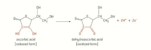
TheconcentrationofvitaminCinasolutioncanbe determinedbyredoxtitrationusingDCPIP (2,6-Dichlorophenolindophenol)asanindicator.Inthe presenceofascorbicacidthepinksolutionoftheprotonated indicatorbecomescolourlessasDCPIPisreduced.As depictedbythischemicalequation:

Figure 2: Molecular depiction of ascorbic acid ina biochemical redox reaction. (Bylikin,Horner,Murphy,&Tarcy2014,p.593)

C12H8NCl2O2 ++C6H8O6 →C12H9NCl2O2+C6H6O6+H+

Duringthetitrationascorbicacidreactswiththetitrant(oxidizingreagent)andthesolutionremainscolourless.Whenthe titrationiscompletealltheascorbicacidisoxidisedtodehydroascorbicacidandthepinkcolouroftheprotonatedDCPIP reappears.Thechemicalequationisdisplayedbelow:

C12H9NCl2O2 →C12H8NCl2O2 + +H+ +2e (Bylikin, Horner, Murphy, & Tarcy 2014, p. 594)

Throughvariousstudies,ithasbeendeterminedthatmanyfruitscontainhighconcentrationsofvitaminCinorganelles suchasthecytosol,cellwallandchloroplasts.“Itreachesaconcentrationofover20mMinchloroplastsandoccursinall cellcompartments,includingthecellwall.”(Smirnoff&Wheeler,2000).Thereforeitcanbeconcludedthatduetothe differencesinfruitstructure,thosewithsimilarstructurewillhavesimilardifferencesinvitaminCmass.However,asthe majorityofthefruitsinthisexperimentarestructurallyuniquetherewillbeasignificantdifferenceinvitaminCmass.

Hypothesis

H1:ThereisastatisticallysignificantdifferenceinthevitaminCmassbetweendifferentfruits.

H0:ThereisnostatisticallysignificantdifferenceinthevitaminCmassbetweendifferentfruits.

Variables

Table 1: Variable Table

Variable Information MethodtoControl/Measure(fordependentvariable)

Independent TypeofvegetablevitaminCis determinedfrom(Orange,Blueberries, RedCapsicum,GreenandYellowKiwi)

Fortheindependentvariable,differentkindsoffruitjuiceswillbeusedforeach subsequentcategorictest.

Dependent MassofVitaminCderivedfromfruit. Tomeasurethemass,theDCPIPredoxtitrationwillbecarriedoutthroughthe stepsinthemethodbeforeusingstoichiometrytodeterminethevitaminC mass.

Controlled Massoffruitusedtomakesolution(g) (±0.01)

VolumeofH₃PO₄ usedtocreatefruit solution(cm3)(±0.5)

Volumeofdistilledwatertowashfruit solutionthroughmuslinfilter(cm3)(±0.5)

Volumeoffruitsolutionthatistitrated (cm3)(±0.04)

Volumeofdistilledwateraddedtofruit solution(cm3)(±0.5)

Molarityofphosphoricacidaddedtofruit solution(2M)

Usinganelectronicbalance(±0.01)themassof50.00goffruit.Thiswillensure thesamemassoffruitisbeingtestedintheindependentvariablesolution.

250cm3 ofH₃PO₄ isaddedtothesolutionandismeasuredwitha250cm3 measuringcylinder(±0.5).Thiswillensurethesolutionsaredilutedequally.

300cm3 ofdistilledwaterisusedtowashthefruitsolutionandismeasuredwith a250cm3 measuringcylinder(±0.5).

Thisismeasuredwitha25cm3 glasspipette(±0.04)beforebeingtitratedagainst DCPIP.WillensurethesamemassesoffruitaretitratedtofindvitaminCmass.

50cm3 ofdistilledwaterisusedtowashthesidesoftheconicalflaskandrinse thetipoftheburette.Thisismeasuredusinga50cm3measuringcylinder(±0.5) beforebeingaddedtothesolutionperiodically.

Thiswillbeensuredandkeptconstantbyusingaconsistentmolaracidforall thetests.SosolutionsareequallyconcentratedandDCPIPreadingsarefair.

Consistentequipmentuse. Throughouttheexperimenttheequipmente.g.glasswarewillbeusedtoensure consistencythroughoutresults.

Method

1.Putonsafetyequipment.

2.Preparematerialsandreagents.

3.Placeaburetteontheretortstandusingaburetteclamp.

4.Placeafilterfunnelatthetopoftheburette.

5.Pour50cm3 (±0.5)ofDCPIPintotheburette.

6.Usinga5cm3 glasspipette(±0.05)measure5cm3 ofascorbicacidintoa conicalflask.

7.TitratetheascorbicacidagainsttheDCPIPindicatorsolutionuntilapink endpointisreached.

8.RecordthevolumeofDCPIPusedinthetitrationinaresultstable.

9.Repeatsteps3to5,fivetimestostandardisetheDCPIP.

10.Placeawatchglassontheelectronicscaleandtaretheweight.

11.Usinganelectronicscaleaccuratelyweigh50.00g(±0.01)ofyellow kiwifruit.

12.Place50.00gofyellowkiwifruitinthefoodprocessor.

13.Usinga300cm3 measuringcylinder,measure300cm3 (±0.5)of2MH₃PO₄

14.Ensurethelidofthefoodprocessorissecurelyattachedandcombineacid andkiwifruit.

15.Usinga300cm3 measuringcylinder,measure300cm3 (±0.5)ofdistilled water.

16.Removethelidofthefoodprocessor.

ScientificDiagram

3: Diagram of Yellow Kiwifruit Vitamin C Determination Set Up

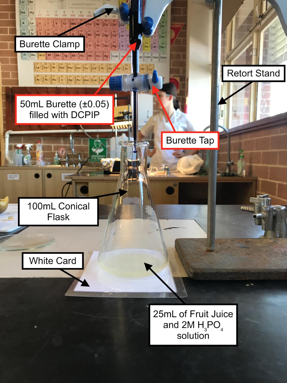
17.Pourthesolutionofacidandkiwifruitthroughasieveusing300cm3 ofdistilledwatertowashthesolutionthrough.

18.Placetheburetteontheretortstandusingtheburetteclamp.

19.Placeafilterfunnelatthetopoftheburette.

20.Pour50cm3 (±0.5)ofDCPIPintotheburette.

21.Usinga25cm3 glasspipette(±0.04)measure25cm3 oftheacidandkiwifruitsolutionintoaconicalflask.

22.TitratethissolutionagainsttheDCPIPindicatorsolutionuntilapinkendpointisreached.

23.RecordthevolumeofDCPIPusedinthetitrationinaresultstable.

24.Repeatsteps10to23,fourmoretimes.

25.Repeatsteps10to23withgreenkiwifruit,yellowcapsicum,redcapsiumandoranges.

26.Cleanupandremovesafetyequipment.

RiskAssessment

Table 3: Risk Assessments

Risk Hazard

Broken Glass ●Cutsfromdamagedorbroken glasstoskin.

Useof 2M

H₃PO₄

●Maycauseharmtotheeyesorina cuttotheskin.

●Causessevereburnsandeye damage.

●Unsafedisposalleadingto environmentaldamage.

Precaution

●Wearsafetyequipmenttoreducethechanceofcutssuchassafetygogglesandlab coats.

●Sweepupbrokenglasswithadustpanandbroom.

●Wearsuchassafetygogglesandlabcoatstoprotecttheskin.

●IfH₃PO₄ comesintocontactwitheyesorcuts,flushwithwaterimmediatelyforatleast 15minutesandremovecontaminatedclothing.

●Washhandsandotherexposedareaswithmildsoapandwaterbeforeeatingand drinkingtoensuresafety.

●H₃PO₄ doesnotposeathreattotheenvironmenthowever,acidshouldbeneutralized withcalciumhydroxideorcarbonatebeforedisposal.

Figure

Table 3: Continued

Risk Assessments

Risk Hazard Precaution

Spilling liquids

Working with electrical appliances

●Slippingandfallingthereforecausing injurytoselforothers.

●Trippingoverunevensurfaces.

●Shocksfromequipmentcancausesevere andpermanentinjuries.

●Faultyoroverloadedequipmentcanlead tofireswhichcancausedamage,injuries andlossoflife.

●Cleanupallspillagesimmediately.Iftheflooriswet,useappropriatesignstotellpeoplethatextracareisneededoruseanotherroute untilthespillageorwetnessisgone.

●Warnofrisksatanychangeinsurface,forexampledrytowet,eventouneven,trafficroutes,byusingsigns,matsormarkings.

●Checkallequipmentisingoodworkingorder.

●Ifyoufindorsuspectafault,stopusingtheequipment,disconnectfromtheelectricalsupplyandlabel'donotuse'.

●Avoidoverloadingsocketsbyprovidingenoughsocket-outlets

●Wherepossibleswitchoffallappliancesatthemainsattheendoftheworkingday

●Switchoffandunplugequipmentbeforeyoucleanitormakeadjustments

●Ensureanaccessibleandclearlyidentifiedswitchislocatednearfixedmachinerytocutoffpowerinanemergency.

Useof DCPIP

●Maybeharmfulbyinhalation,ingestion, orskinabsorption.Maycauseeye,skin, orrespiratorysystemirritation.

●DCPIPmaybehazardoustothe environmentandcauseharm.

●Ensurethatsafetyequipment(safetygogglesandlabcoats)areworn.

●IfDCPIPcomesintodirectcontactwiththeskinoreyes,flushwithwaterimmediatelyforatleast15minutesandremoveany contaminatedclothing.

●DonotingestDCPIP.

●Waftanyscenttoavoidrespiratorysystemirritation.

●EnsurethatallsolutionswithDCPIParecollectedinanorganicwastecollectionandthendisposedofsafely.

Raw

Table 5: Results table for DCPIP volume required totitrate fruit solutions.

TypeofFruitorVegetable

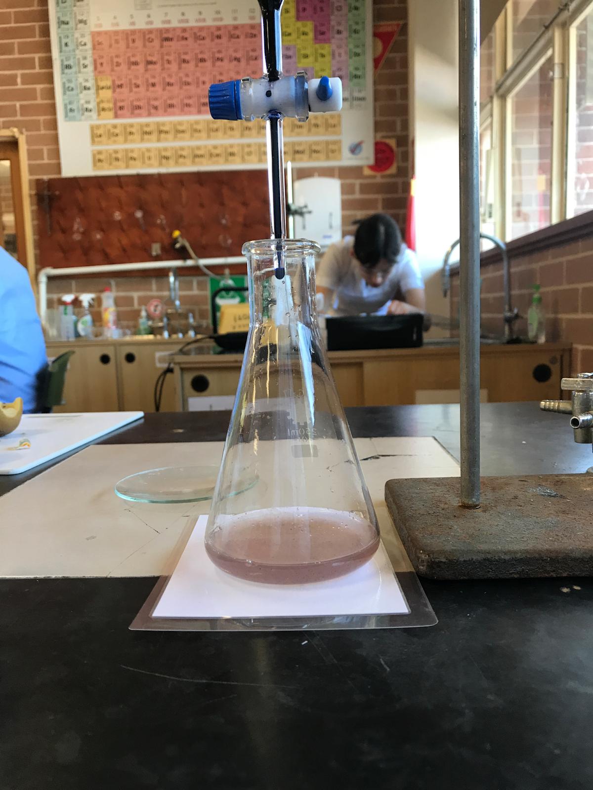
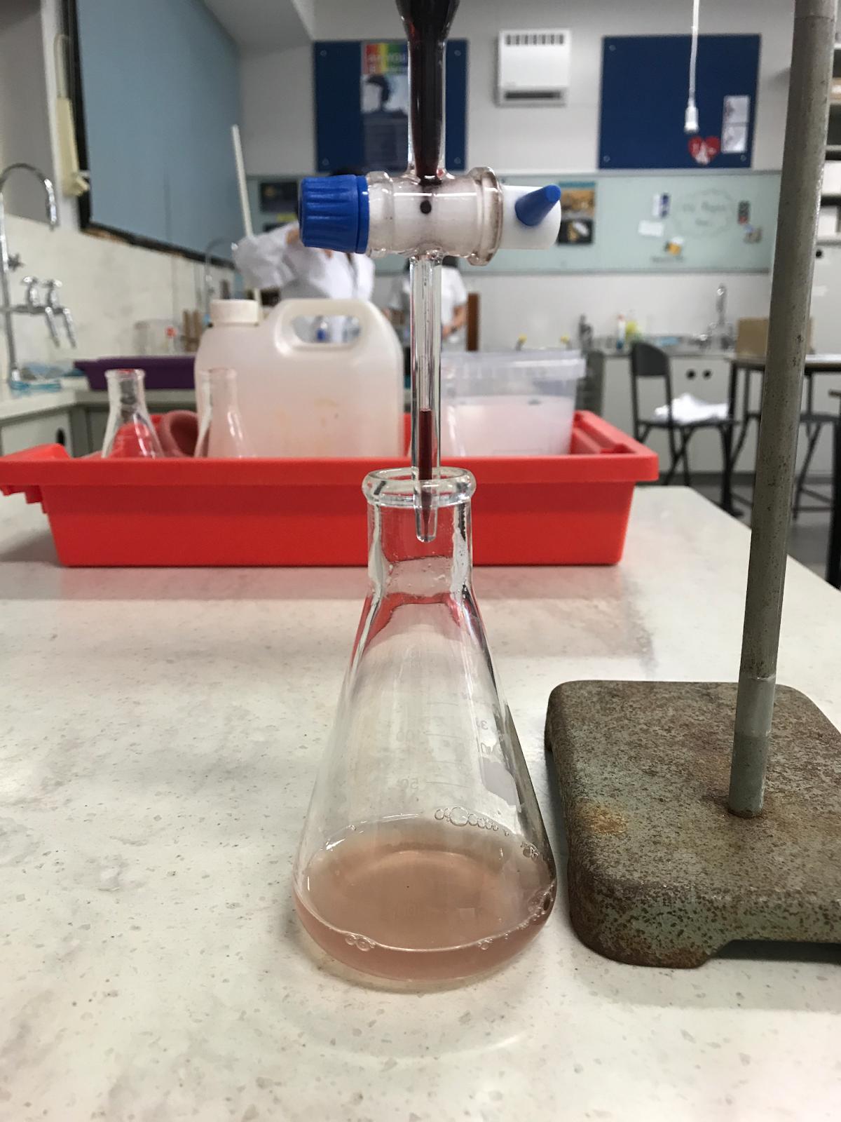
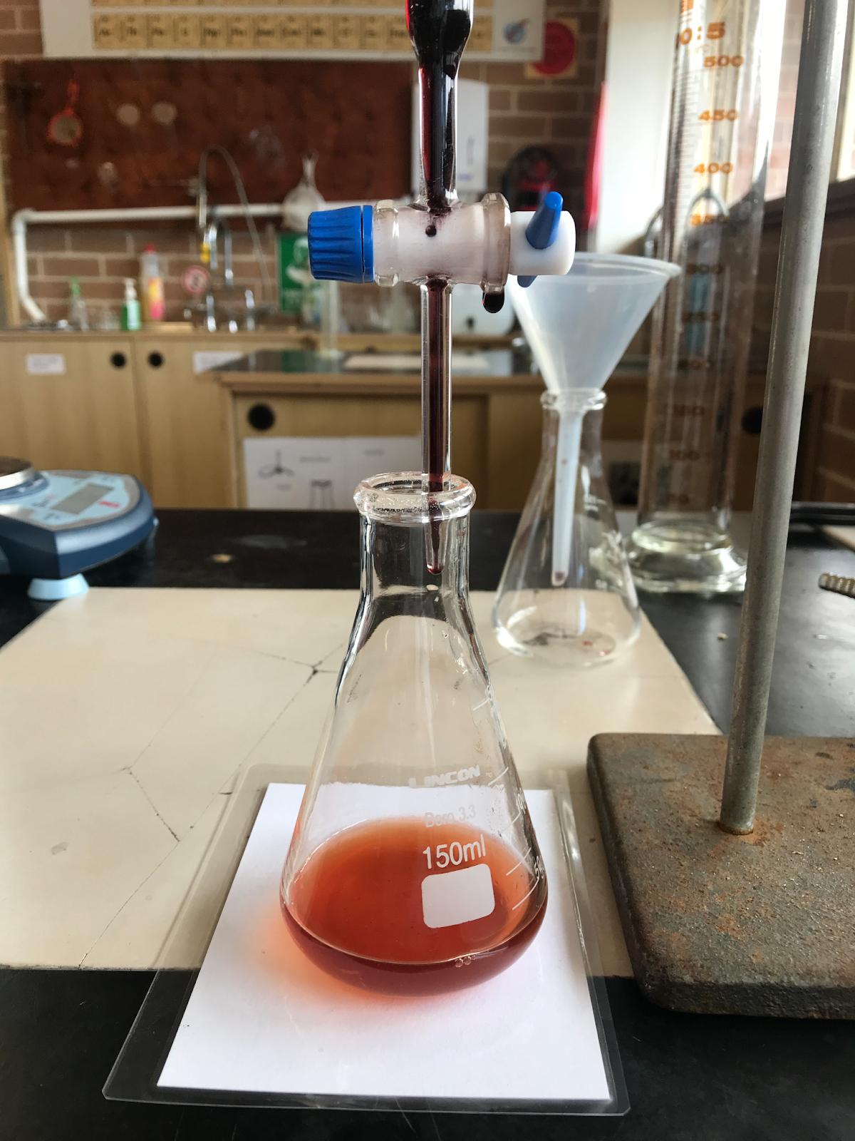
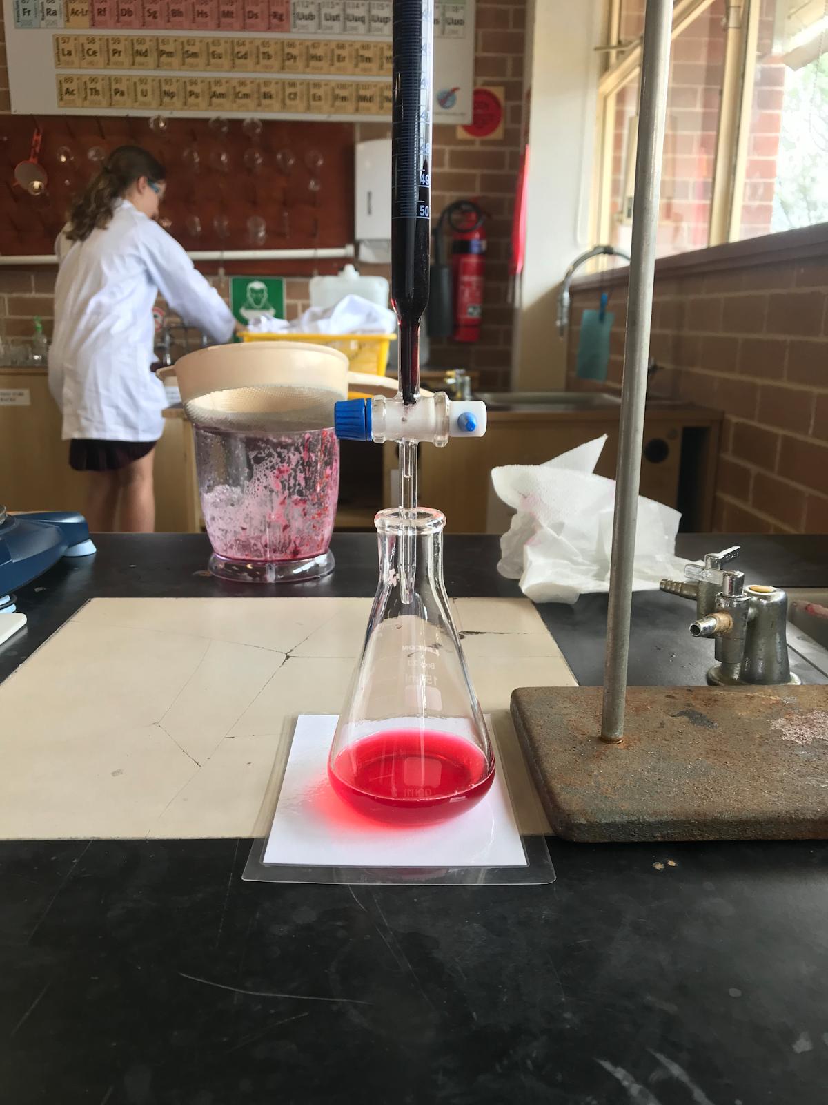
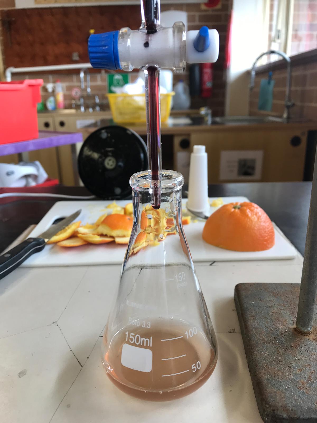
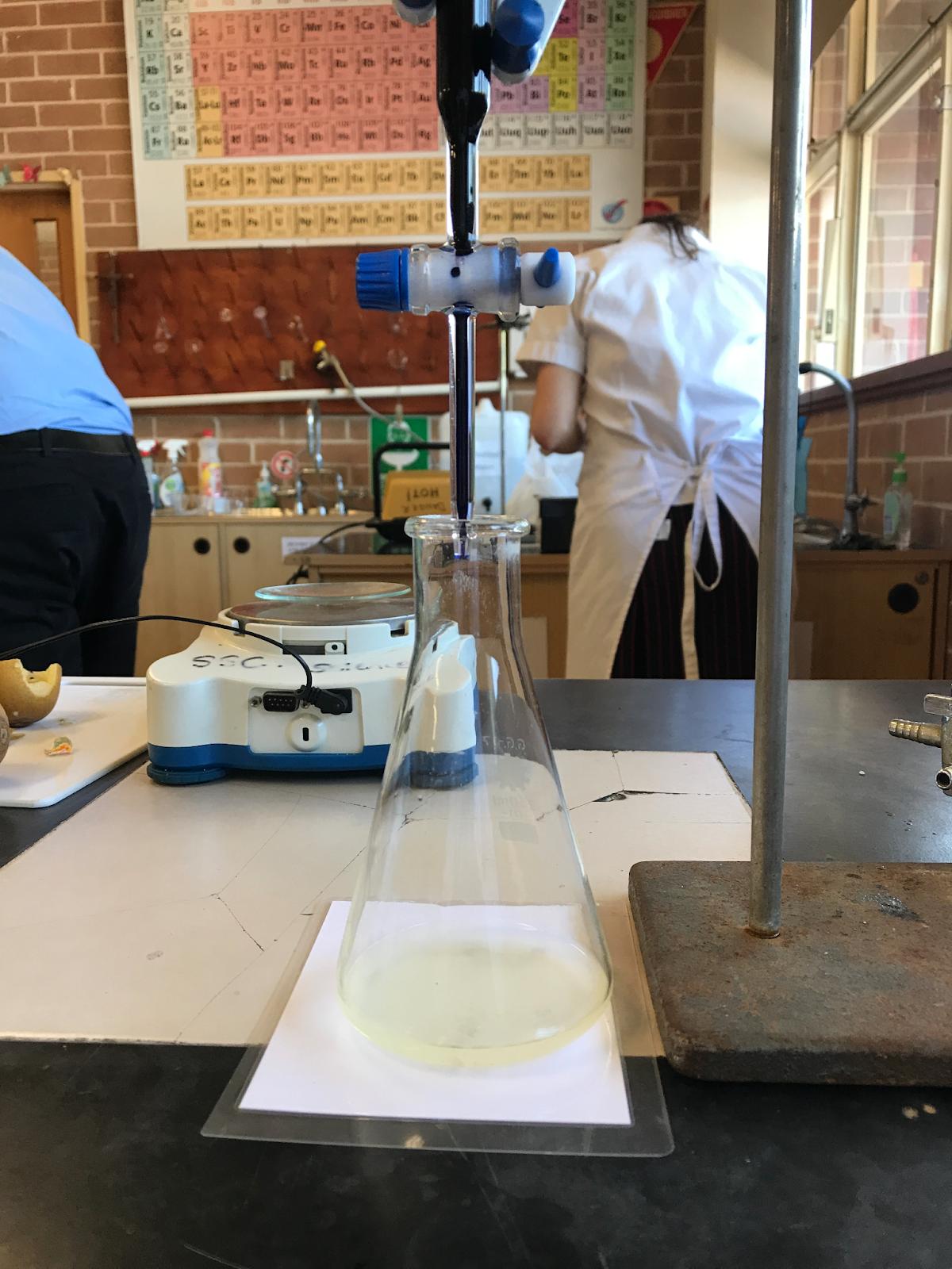
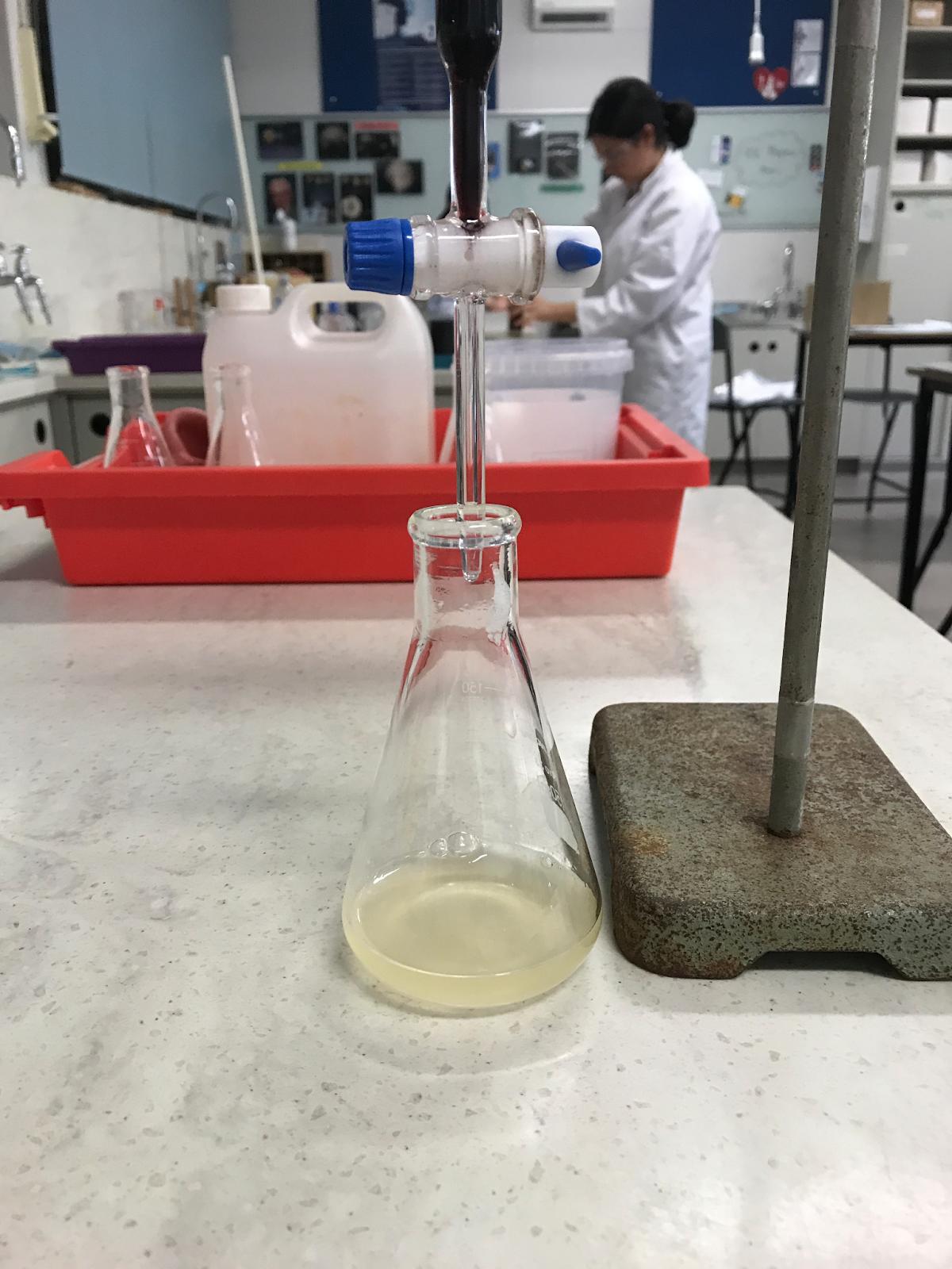
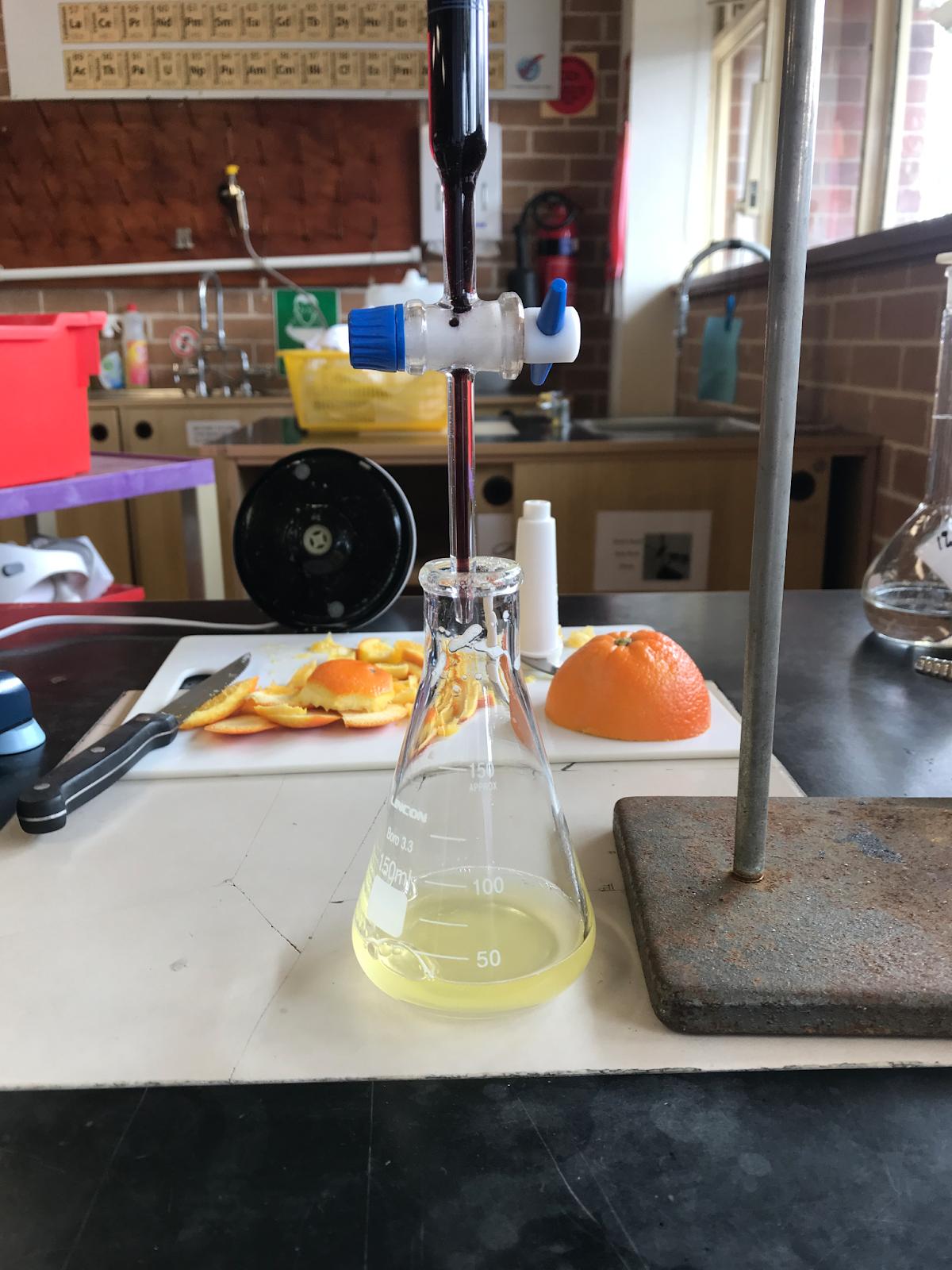
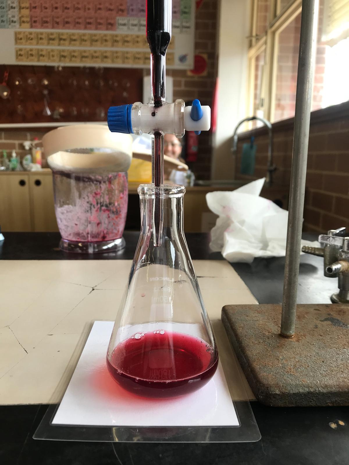
Volume ofDCPIP (mL) (±0.05)

Initial Volume 46.20 45.60 44.90 44.30 43.70 50.00 48.60 47.40 46.20 45.00 50.00 48.20 46.90 45.70 44.80 42.80 42.30 41.70 41.10 40.60 37.40 36.40 35.70 35.00 34.40 Final Volume 45.60 44.90 44.30 43.70 43.00 48.60 47.40 46.20 45.00 43.70 48.20 46.90 45.70 44.80 43.90 42.30 41.70 41.10 40.60 40.00 36.40 35.70 35.00 34.40 33.90

QualitativeData

Table 6: Visual and Written Qualitative Data Depiction.

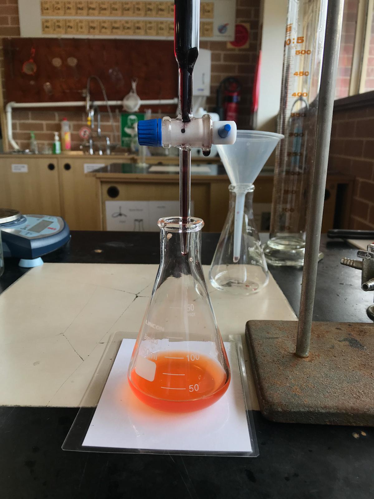
Oranges Blueberries RedCapsicum GreenKiwi YellowKiwi

Initialsolutionwastranslucentand slightlyyellow.AsDCPIPwas added,thesolutionturnedabrown/ purplecolour.

Initialsolutionwasslightlyopaque andred.AsDCPIPwasadded,the solutionturnedamuchdeeperred, purplecolour.

Initialsolutionwastranslucentand brightorange.AsDCPIPwasadded, thesolutionbecameadeeperorange, redcolour.

Initialsolutionwastranslucentand slightlygreen,yellow.AsDCPIP wasadded,thesolutionbecamea brown,purplecolour.

Initialsolutionwastranslucentand yellow.AsDCPIPwasadded,the solutionturnedabrown,purple colour.

ProcessedData

Table 7: Processed Data Table.

TypeofFruitorVegetable

Volume of DCPIP (mL)

Difference (±0.10) 0.60 0.70 0.60 0.60 0.70 1.40 1.20 1.20 1.20 1.30 1.20 1.30 1.20 1.10 1.10 0.50 0.60 0.60 0.50 0.60 1.00 0.70 0.70 0.60 0.50

Average Difference (±0.10) 0.64 1.26 1.18 0.56 0.70

Percentage Uncertaintyof Measurement(%) 15.63 7.94 8.47 17.86 14.29

Standard DeviationError 0.05 0.08 0.07 0.05 0.17

Standard DeviationError Percentage(%) 7.81 6.35 5.93 8.93 24.29

MassofAscorbicAcid(mg) 0.34 0.66 0.62 0.29 0.37

Percentage Uncertainty(%) 16.12 8.35 7.08 18.39 15.44

Propagated Uncertainty 0.055 0.055 0.044 0.053 0.057

Fromthesecalculationsitisclearthatthepercentageuncertaintyofmeasurement(%)islargerthanthestandarddeviationerrorinallcasesotherthaninyellowkiwi.However duetothefurthercalculationstakenwhencalculatingthemassofascorbicacid(seeappendix)ineachfruitthepropagateduncertaintywastaken.Theseerrorbarsarerepresented ingraphs1and2.

StatisticalAnalysis

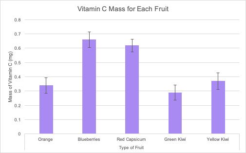
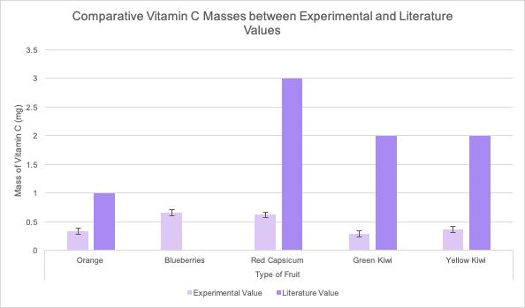
Table 9: One-Way ANOVA Results

ANOVAResultsDetails

Source SS df MS

Between-treatments 2.1304 4 0.5326 F = 47.55357 Within-treatments 0.224 20 0.0112 Total 2.3544 24 P-value is < .00001

Table 10: Student t-Test Results

t-value -13.21844 -12.07477 14.92405 6.03864 13.86362 5.23723

P-value <0.00001 <0.00001 <0.00001 <0.000155 <0.00001 <0.000393

Significance Significant Significant Significant Significant Significant Significant

Analysis

Overallthereisnolineartrendinthedataastheexperimentwascategoricalvariables.Howeverthereweretwo distinctgroupsofhighandlowDCPIPvolumesusedtotitratethevariousfruits.ThefruitsgroupedinhighvitaminC contentare;redcapsicumandblueberries.Withoverlappingerrorbars,itcouldbeconcludedthatthesefruitshave relativelysimilarvitaminCcontentthatwasonlyperpetuatedbythevariouserrorsintheexperiment.Moreover,the highestrecordedmeanvalueoutofthesefruitswasblueberrieswithameanDCPIPvolumeof1.26mLandavitaminC massof0.66mg.Incomparison,fruitswithlowervitaminCcontentindicatedbythevolumeofDCPIPrequiredtotitrate it,includedgreenkiwifruit,yellowkiwifruitandoranges.Thesethreefruitsalsocontainedanoverlapoferrorbarsonall occasionshighlightingthattheresultscollectedbytheexperimentmaybecloserinvitaminCcontentthanindicated. ThroughoutthislowervitaminCcontentgroupthelowestrecordedmeanvolumeofDCPIPwas0.65mLwithavitamin Cmassof0.29mg,fromgreenkiwifruit.ThehighestofthisgroupwasyellowkiwifruitwithameanDCPIPvolume recordedof0.70mLandavitaminCmassof0.37mg.

AsindicatedbythemeanvolumeofDCPIPdataandcalculatedvitaminCmass,blueberrieshavethehighest vitaminccontentandgreenkiwifruithavethelowest.Greenkiwifruit’svolumeofDCPIPrequiredtotitratethesolution was48%lessthanthatofblueberrieswhich,throughstatisticalanalysis,isstatisticallysignificant.Throughthestatistical testofaOne-wayANOVA,itwasindicatedthattheoverallexperimentcreatedasignificantresult.AOne-wayANOVA comparesthemeansoftwoormoreindependentgroupsinordertodeterminewhetherthereisstatisticalevidencethatthe associatedpopulationmeansaresignificantlydifferent.BoththeOne-WayANOVAandtheIndependentSamplest-Test cancomparethemeansfortwogroups.However,onlytheOne-WayANOVAcancomparethemeansacrossthreeor moregroups.BasedontheOne-wayANOVAitwasdeterminedthatthereisasignificantdifferenceinthevitaminC massofdifferentfruits(seetable9).TheOne-wayANOVAindicatesthatthereisaverysignificantdifferencebetween thevitaminCmassofdifferentfruitsasthep-valuecalculatedwas<0.00001.Inbiologythesignificanceleveliswhen thep-valueis<0.05.Thereforethroughthecalculation,theresultcanbeconsideredsignificant.Hence,thisexperiment canacceptthealternativehypothesisof“thereisasignificantdifferencebetweenthevitamincmassesofdifferentfruits”. RejectingthenullhypothesisthatthereisnosignificantdifferencebetweenthevitaminCmassesofdifferentfruits. AfterthecalculationoftheOne-wayANOVA,aposthocTukeyHSDtestwasperformedtodeterminethe internalsignificancebetweengroupsofvariables.Thisconcludedthat6outof10ofthetestscouldbeconsidered significant.IncludingOrange:Blueberries,Orange:RedCapsicum,Blueberries:GreenKiwi,Blueberries:YellowKiwi, RedCapsicum:GreenKiwiandRedCapsicum:YellowKiwi. However,thistestalsocalculatedthatOrange,GreenKiwi andYellowKiwiarevariablesthatdonothaveasignificantdifferencebetweeneachother.Moreover,blueberriesandred capsicumwerealsocategoricalvariablesthatdidnothaveasignificantdifferenceinthevolumeofascorbicacidbetween thepair.ThisstatisticaldifferencewasalsodeterminedthroughtheposthocTukeyHSD.Therefore,forallsignificant

testscalculatedbytheposthocTukeyHSDat-testwascarriedout.Thisdeterminedthep-valueforeachofthesetests andindicatedthesignificanceofthesedifferences.Thesearerepresentedintable10.Thet-testtellsyouhowsignificant thedifferencesbetweengroupsare;inotherwordsitletsyouknowifthosedifferences(measuredinmeans)couldhave happenedbychance.Thetscoreisaratiobetweenthedifferencebetweentwogroupsandthedifferencewithinthe groups.Thelargerthetscore,themoredifferencethereisbetweengroups.Thesmallerthet-score,themoresimilarity thereisbetweengroups.Thet-testformulaisdepictedinfigure5andtheresultsintable10.

Figure 5: t-test formula

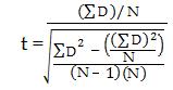
ThelargestdifferenceinthemeanvaluesofDCPIPrequiredtotitrateascorbicacidexistsbetweenblueberries andgreenkiwifruit.Withadifferenceof0.70mLitisevidentthatthereisaverylargedifferencebetweengreenkiwifruit andblueberries'vitaminCmasses.Thisisfurtheremphasisedthroughthecalculationofastudentt-testdepictedintable 9.Throughthiscalculationitwasdeterminedthattheresultwasverysignificantwithap-valueof<0.00001.Therefore highlightingthesignificantdifferencebetweenvitaminCmassesinfruits.

Astandarddeviation(orσ)isameasureofhowdispersedrepeateddataisinrelationtothemean.Forthis experimentaldata,standarddeviationwasbelow0.10forallcategoricalvariablesexceptforyellowkiwifruitThisisdue tothefirsttrialofyellowkiwifruitbeinganoutlier.ThismaybeduetoovershootingthevolumeofDCPIPneededto titratethevolumeofascorbicacidintheyellowkiwifruit.Asitwastheinitialtrial,itwasdifficulttoseewhentheend pointwasreachedHowever,percentageuncertaintyofmeasurementwaslargerthanpercentageuncertaintybasedon standarddeviation.Asrepresentedintheprocesseddatatable(table8).

Conclusion

Duetotheuniquestructuralaspectsofeachindividualfruit,itwashypothesisedthattherewouldbea significantdifferenceinvitaminCmassesacrossthefivefruits.Althoughcorrect,thehypoehtitsesdidnottakeinto accountthefactthattherewouldalsobeinsinginfanctresults.Forexample,duetotheverysimilarstructurebetween yellowkiwifruitandgreenkiwifruit,thep-valuewasconsideredinsignificant.ThiswascalculatedbytheposthocTukey HSDstatisticalanalysis.However,thestructuraldifferencesbetweenthefruitwiththehighestvitaminCcontentandthe lowestvitaminCcontentwasplausible.Theblueberriesandthegreenkiwifruithadverydifferentstructuresandtherefore supportedthealternativehypothesis.Moreover,duetothehighvitaminCconcentrationsinthecellwallofthefruit,the resultofblueberriesasthelargestvitaminCvaluemayhavebeenduetoitbeingtheonlyfruitwiththeskinincludedin thesolutionwhichisgenerallyhigherinvitaminC.Thisisduetothecloserelationshipbetween“theregulationof ascorbatesynthesisandthecellwall”(Fenech,Amaya,Valpuesta,&Botella,2019)hencecellwallsinplantstypically concentratedontheexterioroffruitsarehighinvitaminC.Overall,throughthevariousuniquestructuresofthefruits,the alternativehypothesiswassupported.Moreover,oftenvitaminCisfoundinhigherconcentrationswithinthenatural, lipidaggregatedvesiclescalledliposomeswhicharealsopresentintheliningandphospholipidbilayersofvariousfruits. AstheliposomescontainconcentrationsofvitaminCmass,whentheyareinthesefruitspeciescellwallstheycanbe releasedandhencewhentheskinofthefruitwasintegratedintothesolution,highermassesofvitaminCwerepresent.

Evaluation

Datacollectedthroughtheexperimentshowedtwoseparategroupingsoffruitthatrequiredhighvolumesof DCPIPandthosethatrequiredlowvolumesofDCPIPtobetitrated.ThefruitsthatrequiredhighvolumesofDCPIPwere redcapsicumandblueberries.Basedontheresultscollecteditisclearthatblueberriessupposedlyhadthelargestmassof vitaminC.ThefruitsthatrequiredlesservolumesofDCPIPtobetitratedwereoranges,greenkiwiandyellowkiwi. Further,thefruitthatrequiredtheleastvolumeofDCPIPwasthegreenkiwifruit.Thesegroupsweredeterminedbyan overlapinerrorbars.

Throughouttheexperimentitwasoutlinedthattherewasveryhighpercentageuncertaintyasoutlinedintable 6.Duetothe%uncertaintybeingabovethebiologylimitof<5%itcanbeconcludedthattheexperimenthadlow precision.Toimprovethisinthefuture,usingequipmentwithsmallergraduationswouldhavebeenbeneficial.Duetothe smallvaluesofDCPIPandsolutionsthatwerebeingtitrated,morepreciseequipmentcouldhavehadlowerpercentage uncertaintyoverallandthereforeimproveprecision.Forexample,byhavingaburettewithsmallergraduations,the

percentageuncertaintyoftheDCPIPthatwasexpelledwouldhavebeenlowered,hence,loweringthetotalpercentage uncertainty.

Theresultscollectedwererelativelyreliable.With80%ofstandarddeviationcalculationsbelow0.01,the spreadoverresultsover5trialswasfairlyconsistenthighlightingareliableresult.Thelargeststandarddeviation calculationwasfortheyellowkiwifruitwithavalueof0.17.Thisvaluewasderivedduetotheinitialtrialbeingovershot duetoalackofcolourchangeandconsistentmixingwithinthistrial.Hence,thetrialwasseverelyovershot,leadingtoa largerstandarddeviationvalue.Thesmalleststandarddeviationvaluewasequalbetweengreenkiwifruitandoranges,at 0.05.0.17is240%largerthanthatof0.05,thereforeshowingthatthetestsforgreenkiwifruitandorangesweremuch morereliableastheywereoverallclosertothemean.Overall,throughtheconsistentresultscollectedthroughoutthe trialsoftheexperiment,itcanbeconsideredrelativelyreliable.

Throughthisexperimentitwasdeterminedthattheaccuracyofthisexperimentwasverylow.Throughgraph3, itisclearthattheliteraturevaluesderivedfromtheAustraliangovernmentfooddatastandardsweremuchhigherthan experimentaltestsinallcasesexceptblueberriesandthereforeimpactedwiththeaccuracyofresultswiththelargest percentageerrorof85.50%.Table8,depictsthepercentageerroroftheexperimentdepictingtheinaccuracy.Ifthis experimentwascompletedagain,toimprovetheaccuracy,theintegrationofapHmetertodeterminewhentheendpoint wasreachedcouldbeemployedtoensuremoreaccurateresults.Lowaccuracymayhavebeenduetopoorendpoint determinationthroughvisual,qualitativeinterpretation.Duetodiscrepanciesincolourwhentheendpointwasreached fordifferentfruits,itwasdifficulttodeterminewhenthetitrationhadfinishedandthereforealltheresultswere undershot.Akeyexampleofthisiswiththeblueberrysample.Duetothealreadyred,purplenatureofthemixture,itwas verydifficulttodeterminewhentheDCPIPhadfullyneutralizedtheascorbicacidandthereforetheresultwasundershot. Overall,throughgraph2,itisclearthattheresultsoftheexperimentwerenotparticularlyaccurateduetothelarge percentageerrors,however,themajorityofthefruitsfollowthesametrendastheirliteraturecounterparts,withthe exceptionofblueberries.

Table 11: Table of Errors

SourceofError

Completingthe experimenton differentdays.

Variationsinthe mixingofthe reactants.

Endpoint determination.

Difficultto determinewhen tostoprunning theDCPIP.

TableofErrors

ImpactofError Type MethodtoImproveError

Bycompletingtheexperimentoverseveral daystherewaspotentialfortheresultsto differentdependingontheenvironmental interactions.

Asmixingreactantscanincreasekinetic energyiftheDCPIPandfruitsolutionweren’t mixedthesameamountthetitrationcould indicateafakeendpointandthereforegivean incorrectresultofvitaminCmass.

Asvariousfruitsdepicteddifferentcoloursit wasdifficulttodetermineanendpoint.This mayhaveimpactedtheresultspositivelyor negativelyastheendpointreadmayhavebeen incorrectandthereforethemeasurementof DCPIPwouldbeincorrect.Henceleadingto incorrectvitaminCmassvalues.

Duetothedifferencesanddiscrepanciesin coloursbetweenthefruitjuicesitwas extremelydifficulttodeterminetheendpoint whenaddingtheDCPIP.

Systematic Inordertocontrolthisvariableensurethe experimentiscarriedoutonthesameday.

Random

Inordertoimprovethiserrorensurethatall trialsaremixedthesameamounttoensure consistencyandthereforethesamereaction ofthereactants.

Systematic

Toimprovethis,apilottestofeachfruit usedcouldhavebeenundertakentoidentify whentheendpointwasreached.Therefore, theendpointdeterminationinthefinal experimentwouldhavebeenmoreaccurate, hence,collectedbetterresults.

Systematic

TheadditionofapHmetertodeterminethe endpointofthesolutionwouldbemore accurate.ThepHmeterwouldidentifywhen theendpointisdeterminedthrough quantifiableresultsratherthanbyqualitative interpretation.Thereforethroughthe

Lackofrepeats.

Theexperimentonlycarried5repeatsofeach titration.Whichwaslargeenoughtoanalyse butpotentiallytoosmallforageneraltrend withinafruitspecies.

additionofapHmeter,itwouldbeeasierto determinetheendpointofthetitrationand thereforemakingtheexperimentmore accurate.

Systematic

Toimprovethismorerepetitionsofthe experimentcouldprovidemore representativeresults.Perhaps,further repetitionswouldprovideabettercalculated valueforthemassofvitaminCinthe samplethatwastitratedincomparisontothe muchlowerresultsthatwerecollected.

Implyingthat1g offruit correlated directlyto1cm3 offruitjuice.

Thiserrorinferredthatinthesolutionof H3PO4 andfruitthat50goffruitcorrelated directlyto50cm3.Therefore,whenconsidering the25cm3 sampletitratedineachtrial,only 1.92goffruitwasbeingtitrateddueto calculationsthroughratios.Hence,whentrying tocalculatethemassofascorbicacidinthe fruitthismayhavebeenincorrectas1gofthe fruitmaynotproducemoreorlessthan1cm3 offruitjuice.Therefore,themassesofascorbic acidcalculatedmayhavebeenhigherorlower ifthiswasmorecloselymonitored.

Systematic

Toimprovethiserror,ensurethatwhen blendingthefruitinthefoodprocessorthat itisweigheddirectlyafterandthemassis recordedsothatitcanbecalculatedwhat ratiooffruitjuicethereisinthesolution beingtitrated.

Implyingthat 1.92goffruit wasbeing titratedinevery 25cm3 sample.

Thiserrorimpliedthatinevery25cm3 sample thatwastitrated,1.92goffruitwasbeing titrated.Thiserrormayhaveinterferedwith thefinalvitaminCvalueseitherincreasingor decreasingthisvalueasmoreorlessfruitmay havebeenpresentinthesample.1.92gwas onlychosenasthevalueasinaratiobetween thechemicalsandfruitinthesolution1.92g wasthecalculatedmass.

Random

Toimprovethiserror,makesmallersamples offruitsolutiontotitratesothatitiseasierto recogniseandcalculatehowmuchfruitis presentineachtrial.Hence,making calculationsforvitaminCcontenteasier.

Literature Valueswere onlytothe nearestwhole number.

Thiserrorimpactedtheprocessedandanalysed dataforaccuracy.Astheliteraturevalueswere onlytotheclosestwholenumber,itwas difficulttogagehowclosetheexperimental resultsweretotheliteraturevalue.Especially fortheblueberryvaluewhichgavearesultof 0mg,makingitdifficulttogageapercentage increaseordecreasebetweenliteratureand experimentalvalue.

PossibleExtensions

Random

Toimprovethiserror,findliteraturevalues thatarenotroundedtotheclosestwhole number.

Forthisexperimenttherearevariouspossibleextensions.Firstly,bytestingmorespeciesoffruit,theexperimentalresults coulddepictagreaterspreadofresultsandthereforemoresuccessfullydepictwhetherthereisastatisticaldifferencein vitaminCcontentbetweenspeciesoffruit.Further,throughtheintegrationofapHmeter,theresultscouldbemore accurateastheendpointisnotdeterminedbyvisual,qualitativedata.Moreover,potentiallycomparingthevitaminC contentbetweenfruitsandvegetablesmayhavebeeninterestingtodeterminewhichfoodgroupismoreeffectivein providingvitaminC.

Furthermore,otherexperimentscouldtesthowvitaminCmassinasinglespeciesoffruitdiffersasitisexposed toheat.Byapplyingvarioustemperaturesofheattothesefruitjuicesitcouldbedeterminedatwhattemperatureitis optimumtoeatordrinkfruittoingestthemostvitaminCinanindividual'sdiet.Hence,anotherextensionofthis experimentisusingvaryingtemperaturesofheatappliedtoafruitanddetermininghowthisimpactsvitamincmass overall.

ReferenceList

Britannica,T.EditorsofEncyclopaedia(2018). VitaminC.EncyclopediaBritannica. https://www.britannica.com/science/vitamin-C.

Brown,C,.&Ford,M.(2014). Pearson BaccalaureateChemistry Higher Level 2nd edition.Harlow:Pearson EducationLimited.

Bylikin,S.,Horner,G.,Murphy,B.,&Tarcy,D.(2014). IB Chemistry Course Book: Oxford IB Diploma Programme.Oxford:OxfordUniversityPress CaymanChemical.(2019).DCPIPAssayReagent.RetrievedMarch14th2021,from https://www.caymanchem.com/msdss/700942m.pdf

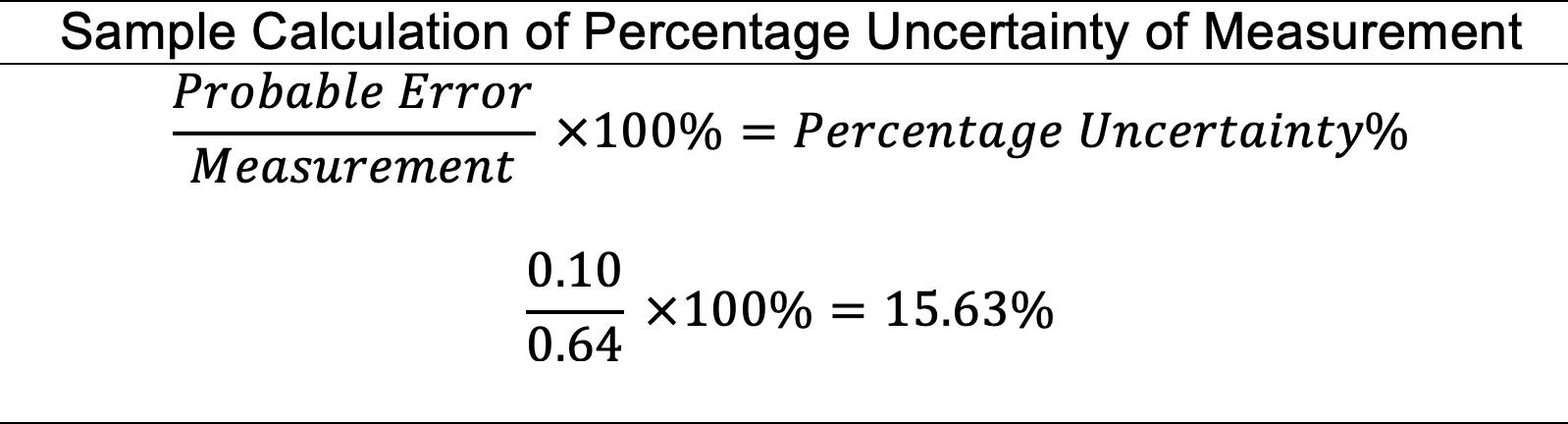
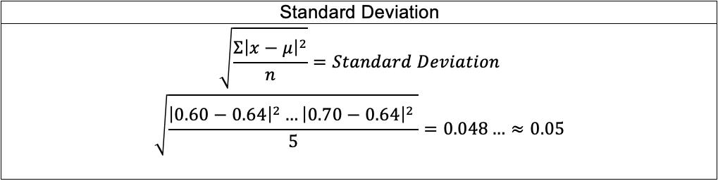
Fenech,M.,Amaya,I.,Valpuesta,V.,&Botella,M.A.(2019).VitaminCContentinFruits:Biosynthesisand Regulation.Frontiersinplantscience,9,2006.https://doi.org/10.3389/fpls.2018.02006

FoodDetails.(2019).RetrievedApril21st2021,from https://www.foodstandards.gov.au/science/monitoringnutrients/afcd/Pages/fooddetails.aspx?PFKID=F006277

FoodDetails.(2019).RetrievedApril21st2021,from https://www.foodstandards.gov.au/science/monitoringnutrients/afcd/Pages/fooddetails.aspx?PFKID=F004815

FoodDetails.(2019).RetrievedApril21st2021,from https://www.foodstandards.gov.au/science/monitoringnutrients/afcd/Pages/fooddetails.aspx?PFKID=F006277

FoodDetails.(2019).RetrievedApril21st2021,from https://www.foodstandards.gov.au/science/monitoringnutrients/afcd/Pages/fooddetails.aspx?PFKID=F002246

FoodDetails.(2019).RetrievedApril21st2021,from https://www.foodstandards.gov.au/science/monitoringnutrients/afcd/Pages/fooddetails.aspx?PFKID=F001290

NicholasSmirnoff&GlenL.Wheeler(2000) AscorbicAcid in Plants: Biosynthesis and Function, Critical Reviews in Biochemistry and Molecular Biology.RetrievedMarch14th2021,from https://www.tandfonline.com/doi/abs/10.1080/10409230008984166 Appendix

BiologySLInternalAssessment

InvestigatingtheEffectofLeafFoliageDensityonRadiantHeat

RESEARCHQUESTION

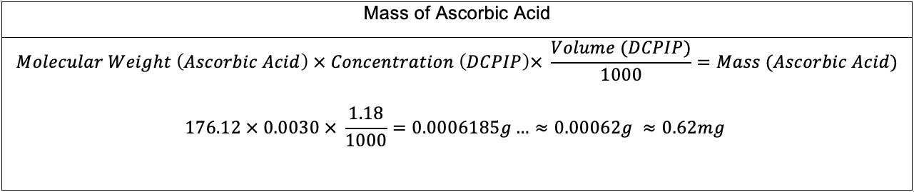
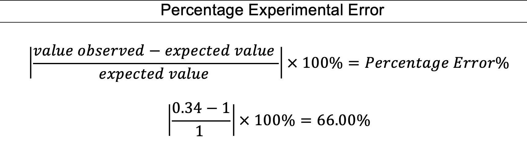
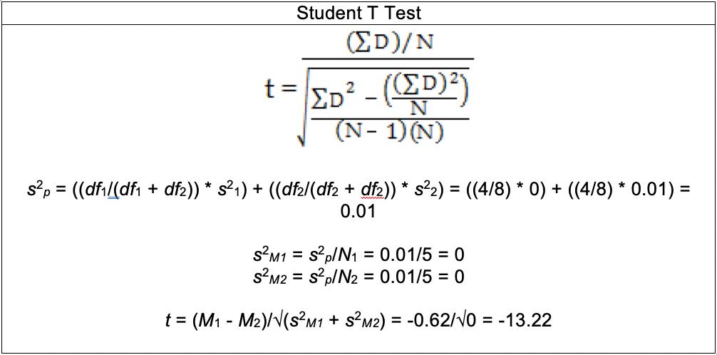
Whatistheeffectofincreasedleaffoliagedensity(0,1and2layers)onradiantheatbelowtheleafcanopy, measuredbyblackglobetemperatureincreaseover10minutes(℃ ±0.1)?

INTRODUCTION

Afterlearningaboutthecoolingcapabilitiesofshadetrees,Ibecameinterestedinaninvestigationintohowtrees canbeusedeffectivelyinurbanareastoprovidecooling,whichisanincreasinglyrelevantareaofscientific research,consideringthecontinuousdevelopmentandexpansionofcitiesacrosstheglobeandrisingtemperatures duetoclimatechange.Theuseoftreesinurbanareasisespeciallyrelevantbecausenotonlyaretheyableto provideshadeandcoolingoutdoors,suchasinparksorurbanforests,buttheycanalsoblocksolarradiationfrom penetratingthewindowsandheatingupthewallsoflarge,urbanbuildings.Aspecificexampleoftheimportance ofurbancoolingistheincreasinglikelihoodofheatwavesandrecord-breakinghotweather,aswellasgenerally highertemperaturesasaresultofglobalwarming.Ithinkitisespeciallyinterestingtoconsidertheuseoftreesto providecoolingincitiesthatnotonlyexperiencewarmweather,butarealsolesseconomicallydeveloped,where luxuriessuchasairconditioningarenotascommon.Conversely,theprevalenceofairconditioninginmore developedurbanareas,whilstcoolingtheinteriorsofbuildings,hastheoppositeeffect,heatingtheairoutside,so thestrategicplantingoftreestopotentiallymitigatethisisalsoarelevantareaofresearch.Anotherinterestingfacet ofthisinvestigationistheexistenceofthe“urbanheatisland”(Ennos,2015).Duringtheday,darksurfacessuchas brickandasphalt,whichareextensivelypresentinurbanenvironments,efficientlyabsorbthesun’sradiantheat energy.Unliketheleavesoftreesthathavenaturalcoolingmechanisms,thesesurfacesreleasethisenergyasheatat night,meaningurbanareascanbeupto7degreesCelsiuswarmerthanthesurroundingcountryside(Ennos,2015). Thus,inlightofthesepotentialpracticalapplications,thisinvestigationseekstodeterminethecoolingcapacitiesof trees’shadecanopy.

BACKGROUNDRESEARCH

Leaveshavevariousradiativepropertieswhichcharacterisetheirradiantheatenergyexchangewiththe surroundingenvironment(Arkebauer,2005).Leaftemperatureiscloselyassociatedwithleafradiantenergy exchange,astheremustbeabalancebetweenenergygainedthroughnetradiationandenergylostthroughvarious processes(Arkebauer,2005).

Theprimarysourceofincomingradiationonaleafissolarradiantheat.Thisistheneitherreflected,absorbedor transmitted(Arkebauer,2005).Energyabsorbedbytheleafitselfcausesatemperaturegainandanassociated reradiationfromtheleafsurfaces.Forthisinvestigation,thesolarradiationtransmittedthroughleavesandtheheat reradiatedfromleavesinthedirectionofthegroundistheheatsourceofinterest,asthisdefinestheperceptible radiantheatloadunderthecanopy.

Theenergytransferredbetweenaleafanditssurroundingscanbedescribedbythefollowingequation,fornet radiationtransferfromincomingradiationandreradiation(Arkebauer,2005):

WhereRn =NetRadiation,Rn’=IncomingRadiation,εleaf =leafabsorptivity,σ=Stefan-Boltzmannconstant,and Tleaf =leaftemperature.

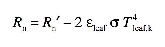
Thisshowshowthereradiationtermdependsstronglyonleaftemperature(varyingwithT4).

Consideringtheenergybudgetoftheleaf,thenetradiationcanbesimplifiedfrom Rn ≈H+λE+S+P, whereSistheenergystoredbytheleaf,andPistheenergyusedforphotosynthesis,to: Rn ≈H+λE, whereHisthesensibleheatflux(conductiveandconvectiveheattransfer)andλEreferstothelatentheatflux(heat lostfromtranspiration),andtermsSandPareneglectedassmall(Arkebauer,2005).

AsfoundbyLin,Chen,Zhang,Fu,&Fan(2017),transpirationisthepredominantmechanismofleafcooling. Inconsiderationoftheaboverelationships,theheatradiationbelowtheleafcanopyishighlydependentonleaf temperature,whichisinturnlargelydependentoncoolingfromtranspiration.

Transpirationistheprocessbywhichwaterinleaftissuesislosttotheatmospherethroughthestomata(Bureauof Meteorology,2021),poresintheepidermisoftheleaf(Allott&Mindorff,2014,p.404).Transpirationisnecessary fortheprocessofphotosynthesis,throughwhichcarbohydratesaresynthesisedusinglightenergy,becauseit requirescarbondioxidetoproduceglucose(Allott&Mindorff,2014,p.404).Tosustainphotosynthesis,carbon dioxidemustbeexchangedwithoxygen,whichisproducedasawasteproduct(Allott&Mindorff,2014,p.404). Carbondioxideisabsorbedthroughthestomata,andinorderforthistooccur,watervapourmustbereleasedfrom theleafandstemintranspiration(Allott&Mindorff,2014,p.404).Plantsalsohaverootsintothesoiltodraw waterandnutrientsintothestemsandleaves(USGS,n.d.).Becauseofwater’scohesiveproperty,duetothe hydrogenbondsbetweenwatermolecules,anditsadhesiveproperty,wherewatermoleculesadheretopolarand hydrophilicsurfaces,watercanbetransportedfromtherootsoftreestotheleavesthroughxylemvessels(Allott, 2014,p.19).

Transpirationinvolvesevaporation,whichisanendothermiccoolingprocess.Energyisabsorbedwhenwater evaporatesandisconvertedfromaliquidtoavapour(Sterling,2004).Thisenergyistransferredfromtheleafto thewatermolecules,whichbecomehighlyenergeticvapourmoleculesandarereleasedintotheatmosphere,and thereforecoolingtheplant(Stirling,2004).Upto99%ofthewaterinleavesislostintheprocessofgasexchange (Babu,2020).

Another,moregeneralaspectofcoolingfromshadetreesisthattreesblocksolarradiationaswellasincreaseair moisture(asdetailedabovethroughtranspiration).Duringtheday,areasthatareexposedtosunlightabsorbheat energy,whichislaterreleasedduringthenight,warmingtheambienttemperatureofthearea.Shadedareas,suchas thosecoveredbytreecanopy,experiencereducedheatradiationduringthedayandhencedonotreleasethe absorbedheatatnight,andthereforehaveacooleraverageambienttemperature(AskNature,2017).

HYPOTHESIS

H1:Thereisasignificantdifferenceintheradiantheatprovidedby0,1and2layersofleaffoliage.

H0:Thereisnosignificantdifferenceintheradiantheatprovidedby0,1and2layersofleaffoliage.

VARIABLES

Independentvariable:Leaffoliagedensity(0,1and2layers)

Dependentvariable:Increaseinradiantheatbelowtheleafcanopy(temperature/time ℃ ±0.1)

Controlledvariables:

Controlledvariable Methodtocontrolthevariable

Lightsource

Positionoflightsource

Temperaturecollectionmethod

Ambienttemperature

Locationofthermometerineachtrial

Sourceofleaves

Cardboardflooring

Orientationofblackbulbthermometer

Measurementintervals

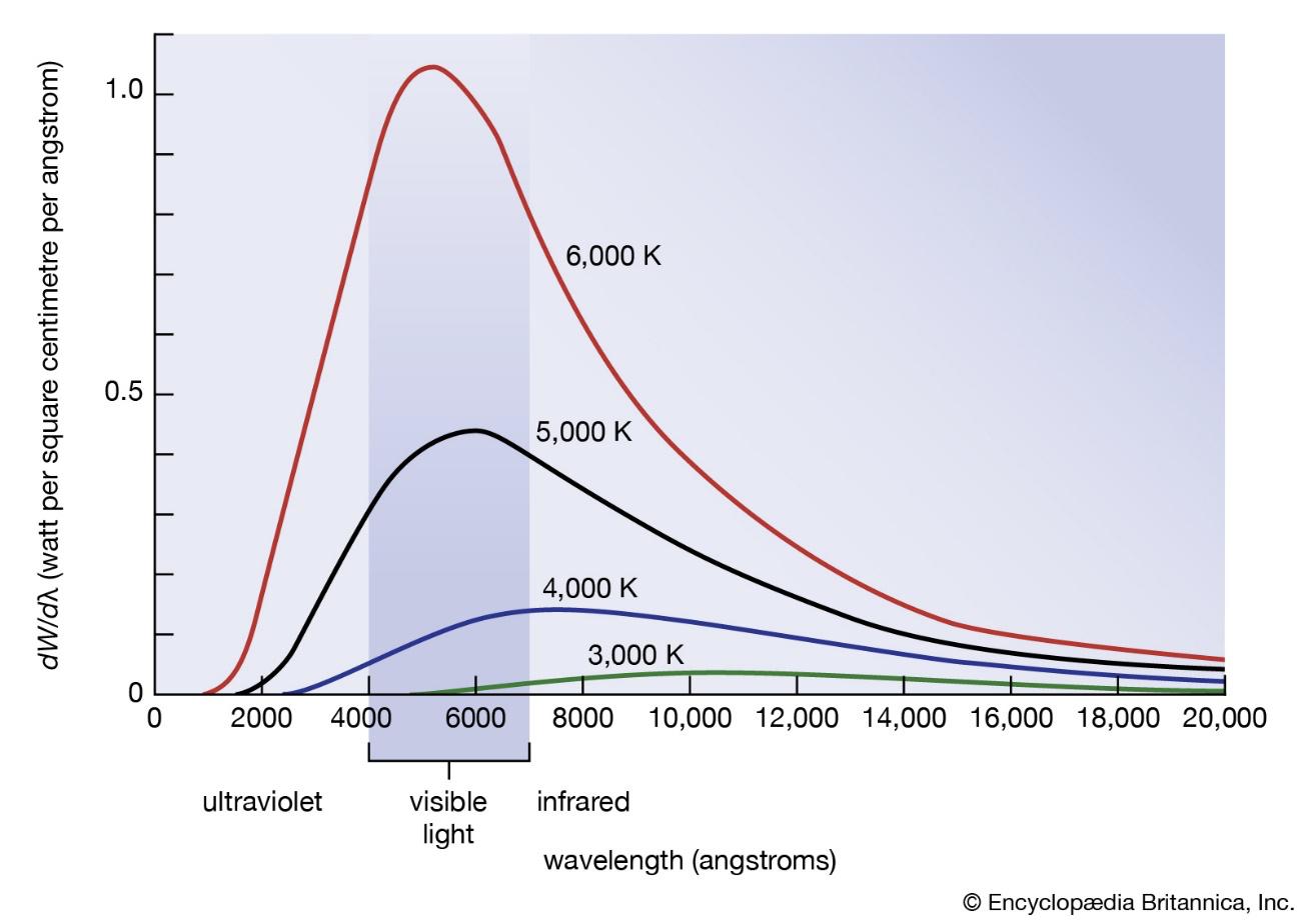
Leaflayerpercentagecoverage

EQUIPMENT

Thesamehalogenlampwasusedforeachtrial.

Thelightsourcewasfixedinplaceabovethegroundbybeing attachedtothetripodstand.Thetripodwasadjustedsothatthe lightwasalways360mmabovethefloor.

Thesameblackgloberadiantheatthermometerwasusedtorecord temperatureduringeachtrial.

Anambienttemperatureof25℃ wasmaintainedforeachtrial.

Thethermometerwaslocatedonthesamepositiononthe cardboardflooring,whichwasdrawnonwithapermanentmarker.

Allleavesweresourcedfromthesamespeciesoftree.

Thesamepieceofcardboardflooringwasusedforeachtrial.

Theblackgloberadiantheatthermometerusedformeasurementof temperaturewasmarkedtoindicatewhichsideofthebulbshould restonthefloor,sothatitwasalwaysorientedthesamewaywhen placedunderneaththefoliagelayer.

Foreachtrial,thetemperaturebelowthefoliagelayerwas measuredaftertenminutes.

Acolouranalysisappwasusedtoanalysethepercentagecoverage ofeachleaflayertominimisedifferencesincoverageaseachnew layerwasconstructed.

Equipment Justification

1xTripod Atripodwasusedtopositionthehalogenlampabovetheleaflayers.

1xHalogenfloodlamp(240V, 500W)

Figure1:Blackbodyradiationatvarioustemperatures(Fritzsche,2016)

1xmetalrack(approximately 200mmx270mminsize)with aheightofapproximately 60mm

1xmetalrack(approximately 200mmx270mminsize)with aheightofapproximately 120mm

Figure2:Leafreflectanceandtransmittance(Arkebauer,2005)

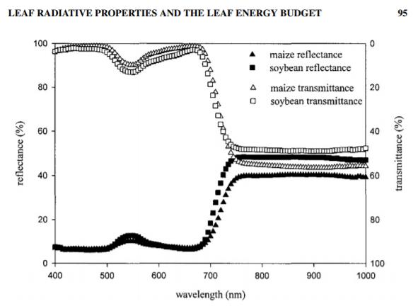
Thehalogenlampisusedtosimulatesolarradiationwithahighintensity artificiallight/heatsource.Duetothedifferenttemperatureofthehalogen elementtothesun,adifferentfrequencyspectrumisproduced(seeFigure1 above)thathasagreaterpercentageofenergyatlongInfraredwavelengths. Asleafenergyabsorptionvarieswithwavelength(seeFigure2above),this sourcedoesnotfullyreplicatenaturallight/heatconditions,butisthebest availablealternative.

Energydensityofsunlightatearth’ssurface:1000W/m2 Therefore,inordertomakethe500Wlight’sintensityroughlyequalto sunlight,thelightmustbeatadistancefromthe“ground”sothatthelight spreadsoveranareaof0.5m2.Afterconductingmeasurements,itwas calculatedthattogetanareaofapproximately0.5m2,thelightshouldbe 360mm(±1mm)fromthefloor.

Theexperimentaldesign,withthemetalrackactingasthebaseforthefoliage layers,waschosenafterpreliminarytesting.Usingtherackswasthemost effectivewaytosimulatemultiplelayersoffoliage,whilststillleavingspace belowforthethermometer.Thisdesignwasreachedafterinitiallyattempting tocreateatree-likestructure,byplacingleavesintoacardboard“trunk”, whichwasunsuccessful.

60xLeaves 60isapproximatelythecorrectnumberofleavesneededtocreatetwoleaf layersonrackswiththedimensionslistedabove.

1xBlackgloberadiantheat thermometer±0.1℃

Ablackglobethermometerisathermometerinsideablackspherewhich absorbsradiantheat.Thetemperaturereadingobtainedequatestotheradiant heatbeingapplied.

30cmofwire Thiswasusedtosecurethelampinplaceonthetripod.

1xA3sheetofcardboardor paper Thiswasusedasaconsistentflooringuponwhichtheleaffoliagewouldbe created.

1xPermanentmarker

Apermanentmarkerwasusedtomakemarkingsonthecardboardflooringto ensurethepositionoftherackswerekeptconsistent.

1xPhoneCamera

Aphonecamerawasusedtophotographeachlayerofleaves,tobeputontoa colouranalysisappforthepercentagecoveragetobecalculated.

1xColourAnalysisApp Thisappwasusedtoensurethatapproximatelythesamepercentageofleaf coverwasachievedeachtimetheleaflayerswerecreatedwithout overlappingtheleaves.

1xTapeMeasure(±1mm) Atapemeasurewasusedtomeasurethedistanceofthehalogenlampfrom theground.

RISKASSESSMENT

Risk Hazard Precaution

Burnstoskin Intenseheatoflight source Lightwashandledwithcaution,attachedhandleswere usedandhandswerekeptawayfromthedirectheatofthe light.Aprominentsafetywarningsignwasalsoinstalled onthelight.

Ethicalrisk Unethicalsourcingof leaves Leavesweresourcedpurposelyfromanon-endangered andnon-nativeplantwithlotsoffoliage.

Environmentalrisk Incorrectdisposalof leaves Allleavesusedintheexperimentweredisposedofafter useintoagardenorganicsbin.

METHOD

1.Gatherequipment.

2.Removearound20leavesfromthechosenplantandbringbacktothelab.

3.PlaceanA3sheetofpaper/cardboardontothefloorofthelab.

4.Traceusingapermanentmarkertheshapeofthemetalrackontothecardboardpiece,aligningthemiddle oftherack’spositionwiththepositionofthelamp.

5.Tracealsothepositionoftheblackglobethermometertobeplacedbelowtherack.

6.Set-upthetripodoverthecardboardsheetandcarefullyattachthelightsource(halogenlamp)after measuringheightwithatapemeasure,usingwiretosecureitinplace360mmabovethepaperflooring.

7.Placeblackglobethermometeronitsdesignatedpositiononthefloor.

8.Turnonthelampandstartthestopwatchsimultaneously.

9.Measureandrecordtheradianttemperatureaftereveryminutefor10minuteswhenthethermometeris exposedtodirectlightandthereiszerofoliage.

10.Repeatsteps8and9fourtimesafterthethermometerhasreturnedtoroomtemperature(around25℃).

11.Placealayerofleavesovertheshortermetalracksothatitssurfaceisentirelycovered.

12.Usingaphoneorcamera,takeaphotooftherackofleaves.

13.Inthephoto’ssettings,turntheexposureto100,thecontrastto80andthesaturationto-100.

14.Usingacolouranalysisapplication,uploadtheeditedphotooftheleaves,croppingtheimageuntilonlythe rackisvisible.

15.Recordthepercentageofcoloursthatcorrespondtotheleavesinthephoto.

16.Gentlymovethemetalrackwithoneleaflayertoitsdesignatedpositionabovethethermometer.

17.Oncethethermometerhasreturnedtoitsinitialtemperature(25℃),turnonthelampandstartthe stopwatchsimultaneously.

18.Measureandrecordtheradianttemperatureaftereveryminutefor10minutes.

19.Repeatsteps17and18fourmoretimesafterthethermometerhasreturnedtoinitialtemperature(25℃).

20.Repeatstep11,insteadplacingleavesoverthetallerrack.

21.Repeatsteps12to15withthe2ndfoliagelayer.

22.Carefullypositionthetallerrackwitha2ndfoliagelayerovertheoriginalrack(1stfoliagelayer).

23.Repeatsteps17and18fivetimeswiththetwofoliagelayers,eachtimeafterthethermometerhasreturned toitsinitialtemperature(25℃).

Photographofset-up:

RESULTS

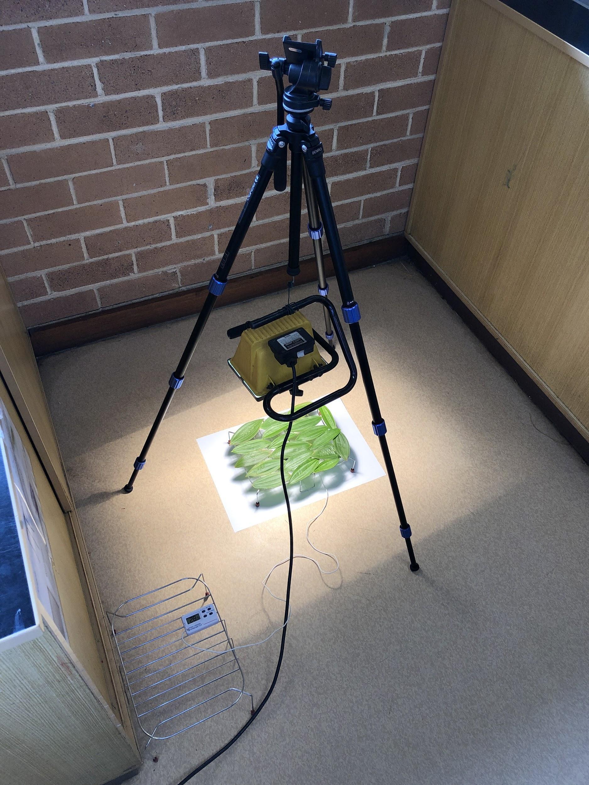
Rawdata

LayersofLeaves Changefromstarttemperaturetofinaltemperature(℃ ±0.1)

Trial1 Trial2 Trial3 Trial4 Trial5

0 6.6 6.9 5.6 6.5 6.1 1 4.6 4.8 4.1 3.5 2.7 2 1.2 0.9 1.4 1.7 1.4

Processeddata

Layersofleaves Averagechangein temperature (℃ ±0.1)

Standarddeviation %uncertaintyof measurement %uncertaintyof repeats

0 6.3 0.450 1.59 7.14 1 3.9 0.766 2.56 19.64 2 1.3 0.264 7.69 20.31

QualitativeData

Becausetheexperimentwasconductedoverdifferentdays,andtheleaveshadtobefresheachtime,acolour analysisappwasusedtocalculatethepercentagecoverofleavesforeachlayerthatwascreated,attemptingto reachasimilarlevelofcoverageeachtimetomaintainconsistency.Eachphotowaseditedwithhighexposureand contrastandzerosaturationtomakeitclearerforthecolourapptodistinguishbetweenleavesandnon-leave substancessuchasgapsbetweenleaves.Exposurewassetto100,contrastwassetto80,andsaturationwassetto

-100.Thefollowingeditedphotosshoweachleaflayer,atotalofsix,whichwascreatedforthedifferenttests. Percentagecoveragevaluesrangedfrom73.92%-79.16%,withanaverageof

Graph

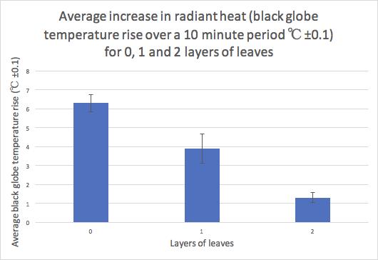
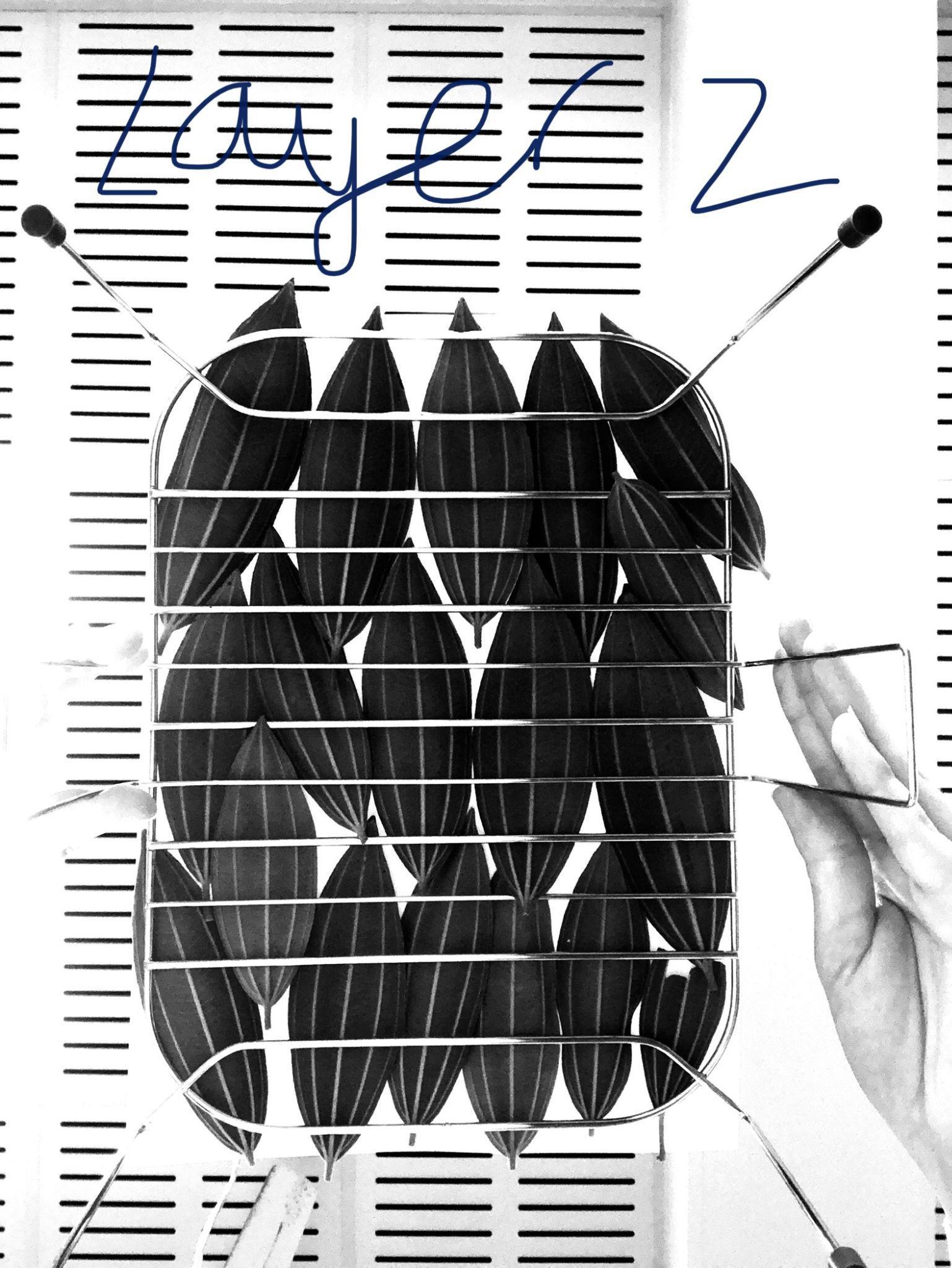
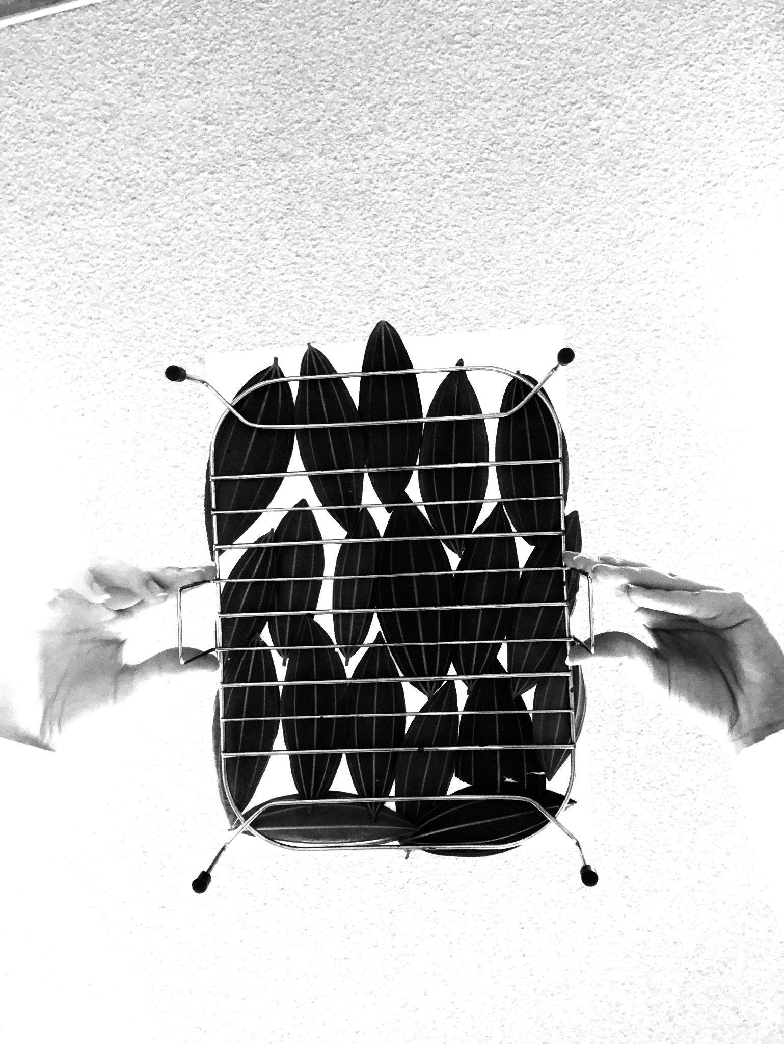
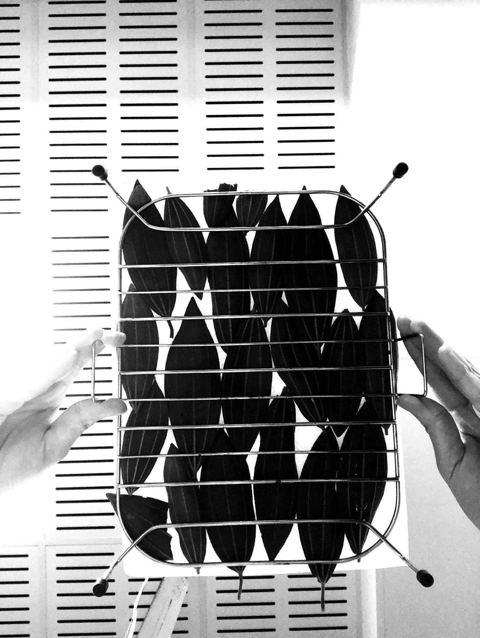
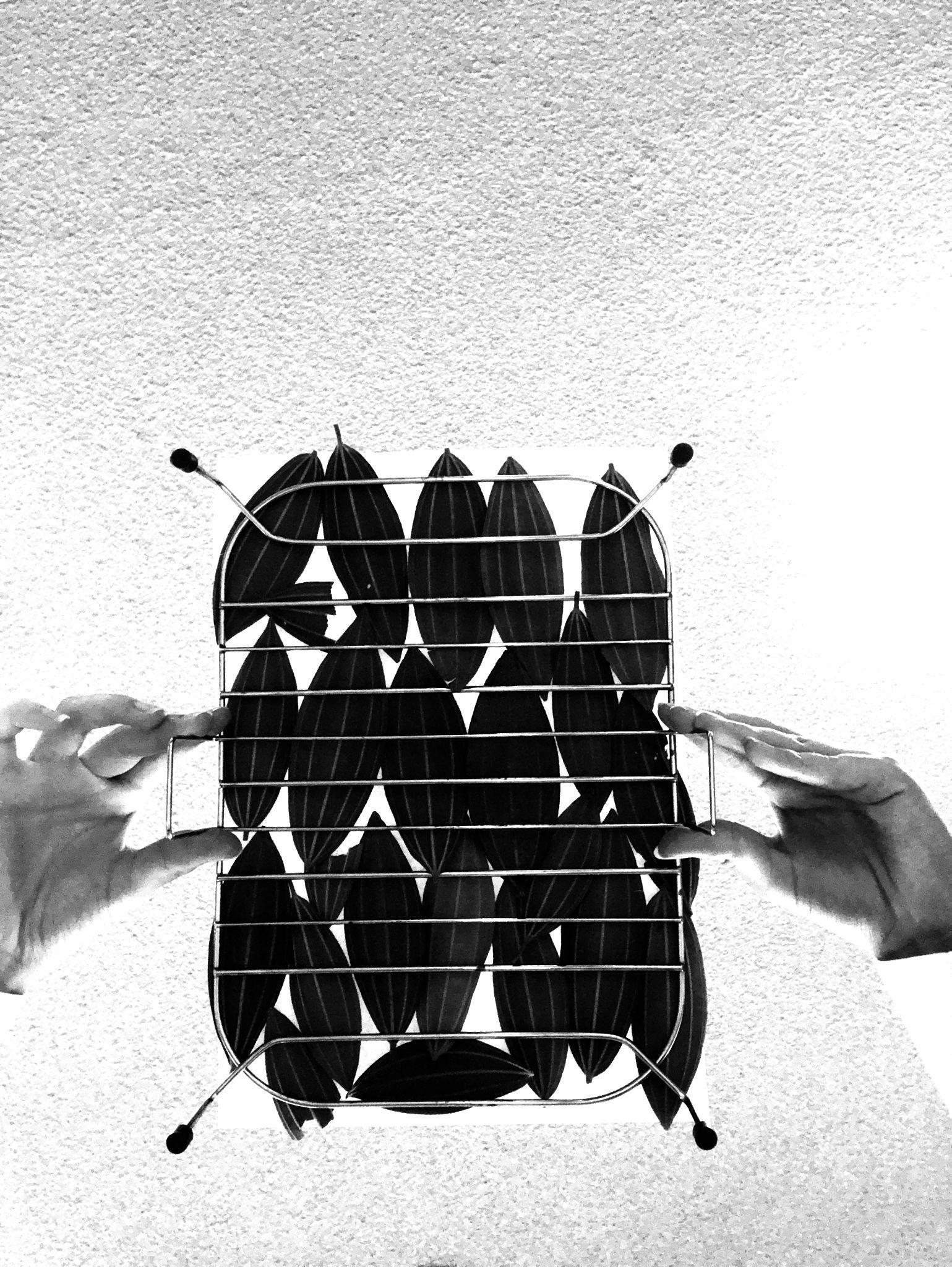
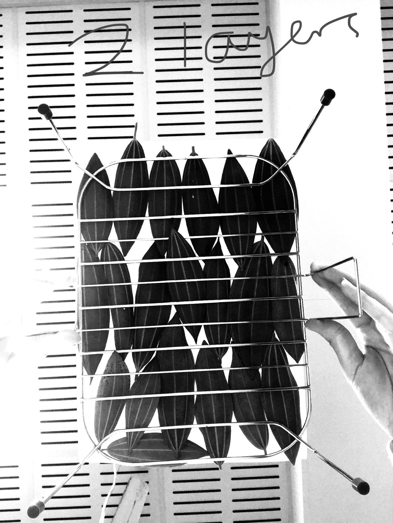
Acolumngraphwasusedtodisplaythedatacollectedinthisexperiment,toreflectthecategoricalnatureofthe independentvariable.

Statisticaltest

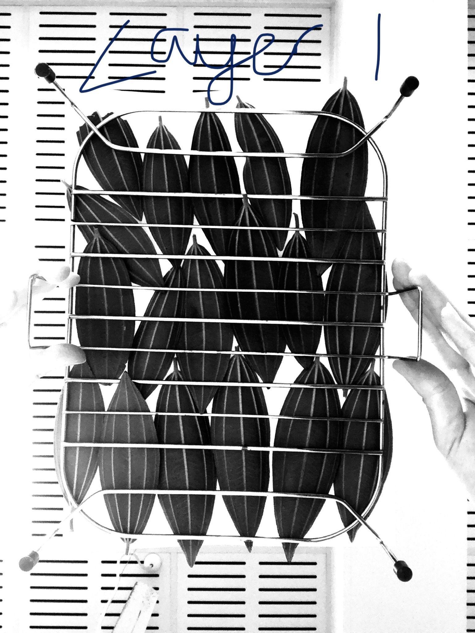
At-testfortwoindependentmeanswasconducted,toestablishiftheresultsarestatisticallysignificant,by determiningtheconfidencelevelinthehypothesis.Thist-testwasusedbecausethisexperimentinvolvesthe comparisonof3separate,independentsamples-0,1and2leaflayers. T-testequation:

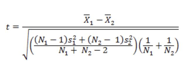
T-testfor0layersand1layer: Meandifferenceintemperature:2.4℃ s2 p =((df1/(df1 +df2))*s2 1)+((df2/(df2 +df2))*s2 2)=((4/8)*0.25)+((4/8)*0.73)=0.49 s2 M1 =s2 p/N1 =0.49/5=0.1 s2 M2 =s2 p/N2 =0.49/5=0.1 t=(M1 -M2)/√(s2 M1 +s2 M2)=2.4/√0.2=5.4 The t-valueis5.40453.The p-valueis.000321.Therefore,theresultissignificant(p<.05).

T-testfor0layersand2layers:

Meandifferenceintemperature:5.0℃ s2 p =((df1/(df1 + df2))* s2 1)+((df2/(df2 + df2))* s2 2)=((4/8)*0.25)+((4/8)*0.09)=0.17 s2 M1 = s2 p/N1 =0.17/5=0.03 s2 M2 = s2 p/N2 =0.17/5=0.03 t =(M1 M2)/√(s2 M1 + s2 M2)=5.02/√0.07=19.25

Thet-valueis19.25082.Thep-valueis<.00001.Therefore,theresultissignificant(p<.05).

T-testfor1and2layers:

Meandifferenceintemperature:2.6℃ s2 p =((df1/(df1 + df2))* s2 1)+((df2/(df2 + df2))* s2 2)=((4/8)*0.73)+((4/8)*0.09)=0.41 s2 M1 = s2 p/N1 =0.41/5=0.08 s2 M2 = s2 p/N2 =0.41/5=0.08 t =(M1 M2)/√(s2 M1 + s2 M2)=2.62/√0.16=6.47

The-valueis6.46963.Thep-valueis.000097.Therefore,theresultissignificant(p<.05).

The3t-testseachhaveapvalueoflessthan0.05,sothereisasignificantdifferenceinthetemperaturechange betweeneachincreasedlayerofleaves.Therefore,thenullhypothesisisrejectedinfavourofthealternative hypothesisthatthereisasignificantdifferenceinthereducedradiantheattransmissionprovidedbyaleaffoliage shade,withaveryhighconfidencelevel.Furthermore,thistestrevealsthatnotonlyis1leaflayerbeneficialin reducingtemperature,butsoare2leaflayers,asthepvalueforthet-testbetween1and2layersisalsosignificant, leadingtotheconclusionthatnotonlydoesfoliagedensityreduceradiantheattransmission,butincreasedfoliage enhancesthiseffect.

DISCUSSION

Analysis:

Descriptionofresults

Asthenumberofleaflayersincreased,theradiantheatinverselydecreased,asmeasuredbythedecreasingblack globetemperaturerise.Forthecontrolof0layers,theaverageblackglobetemperaturerisewas6.3℃,but decreasedtoa3.9℃ risefor1layer,andagaintoa1.3℃ risefor2layers.Theheatradiationwasreducedby2.4℃ from0to1layers,andby2.6℃ from1to2layers,andatotalreductionof5℃ from0to2layers.Evaluatingthe changeonaproportionalbasis,from0to1layers,therewasa38%reductionintemperaturerise,from1to2 layers,therewasa66%reductionandtherewasanoverallreduction,from0to2layers,of79%.Thisshowsthat theadditionof1layerofleaveshasapronouncedeffectonradiantheat,buttheeffectofanaddedsecondlayeris evengreater.Thetotalreductioninradiantheatachievedwith2layers,ofalmost80%,isconsiderable.

Thegraph’sverticalerrorbarsshowthestandarddeviationforeachsetofvalues,thelargestrawerrorforthe experiment.For0leaflayers,thestandarddeviationwas0.450.For1leaflayer,thestandarddeviationwashigher at0.766.2leaflayershadthesmalleststandarddeviationof0.264.Theerrorbarsdonotoverlap,whichincreases confidenceintheresults.

Thepercentageuncertaintyofrepeatswasalsocalculated,bydividingthestandarddeviationforeachvariableby thedatavalueandthenmultiplyingitby100.For0layers,therewas7.14%uncertainty,for1layertherewas 19.64%uncertainty,andfor2layerstherewas20.31%uncertainty.Thesevaluesareallgreaterthan5%and thereforetheerrorinvolvedinrepeatscanbeconsideredlarge,especiallyfor1and2leaflayers.

Explanationofresults

Theresultsofthisexperimentshowblackglobetemperatureriseover10minutesfor0,1and2leaflayers, representingthechangeinradiantheatbelowtheleafcanopy.Thelargereductionintemperatureincreasebetween eachsuccessivelayerisindicativeoftheuseofashadecanopybeingveryeffectiveinreducingradiantheatload, andthereforecoolingthespaceandsurfacesunderneath.Furthermore,itcanbeseenfromtheresultsthatincreased foliagedensityconsiderablyenhancesthiseffect,thereforeindicatingthatadenser,multi-layeredcanopyismost effective.

Thebackgroundresearchidentifiedthattheradiantheatisacombinationoftransmissionandreradiationbythe leavesoftheincomingradiantenergylessthesensibleandlatentheatlosses,ofwhichthedominantcooling mechanismislatentheatlossduetotranspiration.Inconsideringtheeffectofthesecondleaflayer,itisproposed thattheincomingradiationtothatlayerisreducedbythemeasuredreductionofonelayer,38%,butthe transpirationheatlossisofasimilarmagnitudeineachlayer,evidencedbysimilarΔT,thereforeproducinga greaterproportionalreductioninthesecondlayerthanthefirstlayer.

Thecontributionofdirecttransmittanceofradiationthroughtheleaflayerisalsoaconsideration.Whilst transmittancethroughindividualleavesisassumedtobelow(likemostopaquematerials),theaveragelayer coverageofaround77%allows23%transmittanceofheatradiation.Assumingrandomgapdistribution,the transmittancethrough2layersisreducedto5%(0.23x0.23=0.053),sotransmittedradiationisalsogreatly reducedasaheatsource.

Theprocessoftranspirationcontributestothecoolingeffect,aswaterinleaftissuesisconvertedintoavapourand losttotheatmospherethroughthestomata.Thiscoolstheareaaroundthefoliagebecausethelossofenergy involvedintranspirationisgreaterthantheenergyusedintheconversionofwaterfromaliquidtoavapour.

Preliminarytestingindicatedthataddinga3rdlayerofleaveswouldnothaveasignificantlydifferentreductionin radiantheattransmissioncomparedto2layers.Whilstthiswasnottestedexplicitlyinthisinvestigation,these resultsshowthat2leaflayersprovidelargelyreducedradiantheattransmission(-79%)comparedto0leaflayers, buttherelikelywouldnotbeasignificantdifferencewith3layerscomparedto2,as79%oftheoriginalheat radiationhasalreadybeenprevented,andthesmallremainingheatradiationislikelytoincludeotherpathssuchas surroundingreflections,duetotheexperimentdesign.

Evaluation:

Thepercentageuncertaintyofmeasurementrevealstheprecisionoftheequipmentusedintheexperiment.This uncertaintywasbelow5%forboth0and1leaflayers,butincreasedto7.69%for2leaflayers.Overall,therewasa lowerrorofmeasurementandsothedatacanbeconsideredprecise,althoughthe2leaflayersweretheleast preciseofthethree.

Theinternalreliabilityoftheexperimentisgivenbythepercentageuncertaintyofrepeats.For0layers,thereis 7.14%uncertainty,for1layerthereis19.64%uncertainty,andfor2layersthereis20.31%uncertainty.Eachof thesevaluesaregreaterthan5%,andtheuncertaintyfor1and2layersisparticularlyhigh.Theexperiment thereforehassomewhatlowreliability.Theexperimentaldatawasalsolimitedduetothefactthatonly5trials wereconductedforeachtest,andsoabiggerdatapoolwithmoretrialswouldhaveincreasedtheinternal reliability.

Error Detail

Systematic Useofblackglobe thermometerwith readingsto1decimal place

Random Intrinsicvariability

EffectonExperiment MethodtoMinimiseImpact

Whilsttherewasnoevidenceof systematicerror,itispossiblethat thethermometerused,providing temperaturestoonly1decimal place,couldhaveincreasederror.

Intrinsicvariabilitywasone randomerror,astheexperiment wasconductedoverdifferentdays andinslightlydifferentlocations, whichcouldhaveincreasedthe variabilityofresults.Variability wasalsopresentintheuseof leaves,asnewleaveshadtobe usedforeachseparatedayof testing,andnaturalvariationwas presentamongstleafsizes,shapes andsurfacearea.

Theuseofamoreprecisedigital temperatureprobeabletoprovide temperaturereadingswithmore decimalplaceswouldreduceerror andlikelyyieldbetterresults.

Whilstattemptsweremadeto mitigatethisvariabilityby calculatingthepercentage coverageofeverynewlayerand tryingtoensureeachlayerhada similarpercentage,muchofthis randomerrorisdifficultto control.Thatbeingsaid,itis usefultobeawareofthepotential impactonresultsofusingorganic materialssuchasleaves.This inherentvariabilitycouldalsobe reducedbyconductingfurther testingoveralongerperiodof time.

Random Variationinheatfrom thelightsource

Becausethelampwasswitched onandofffortenminuteperiods repeatedly,itispossiblethatthere wassomeinherentvariationinthe heatprovided.

Multipletrialswereconductedto reducethiseffect.Alongertime betweentrialswouldgivemore consistentthermalconditionsfor eachtrial.Inputconditions includingactuallivevoltage couldalsobemeasured.

Random Variationinheightof thelampusedasalight source

Thelamphadtobere-positioned foreachnewdayoftestingand thereforecouldbepositionedata slightlydifferentheightfromthe setupeachtime

Whilstitwasimpracticalforthis experiment,ideally,thetests wouldallbeconductedduringthe sametimeperiodtoavoiderrors insettingup.Amoreprecise holdingmethodandmeasurement toolcouldalsobeusedfor measuringtheheightofthelamp eachtime.

Theoverallaccuracyofthedataisrelativelyhighthough,asthereisnoovertsystematicerrorandagenerallyhigh precision.Thet-testforindependentmeansshowedthattherewasasignificantdifferenceinresultsforeachofthe leaflayertests,furtherindicatinghighaccuracy.Theoveralltrendsoftheresults,showingveryclearreductionsin temperaturerisebetween0and1leaflayers,and1and2leaflayers,arealsoindicationsofaccuracy,asthese correspondstronglytowhatwaspredicted.

Theexperiment’svalidityisgenerallyquitehigh,astheresultsrespondeffectivelytotheexperiment’saimandboth precisionandaccuracyarequitehigh.Thestatisticaltestalsoshowedthattheresultsaresignificantbetweenboth0 and1layers,1and2layers,and0and2layers.Furthermore,thestatedvariableswerecontrolledeffectively,as

Candidatecode:hzy524 detailedinthetableoutliningmethodtocontrolvariables,andnootherconfoundingvariableswereidentified, furthercontributingtothevalidityoftheresults.

Thereweresomelimitationstothisexperimentwhichcouldbeimprovedwithsomeextensions.Firstly,thescope oftheexperimentcouldbebroadenedtoexploremorethoroughlythegeneralimpactofshadestructureson cooling.Forexample,comparativetestingcouldbeconductedusingnon-organicshadestructuresinsteadofleaves, suchaslayersofpaperorcardboard,todeterminemoreclearlyifthecoolingeffectwastheresultoftheparticular useofleaves,orislimitedjusttoshadestructuresingeneral.Comparisonscouldalsobemadetonon-organic shadestructureswithevaporativecoolinglikeleaves,todetermineifthishasanyeffectoncoolingproperties.Tests couldalsobeconductedwithavarietyofdifferenttypesofleaves(plantspecies)toexplorethedifferencesin resultswithleavesofdifferentcolours,shapes,sizes,thicknessesortextures.Anotherpossibleimprovementwould betoalsomeasurethesurfacetemperatureoftheleavesateachlayer,todetermineifthereisatruecorrelation betweenleaftemperatureineachlayerandreradiation,aswasindicatedinthebackgroundresearchbytheequation fornetradiationtransfer.Overall,themajorityofthesesuggestedextensionsreflectthepotentialbenefitsof deepeningtheinvestigationtoexplorethewidercoolingcapabilitiesofshadestructures,differenttypesofleaves, andtobetterunderstandtherelationshipbetweenleaftemperatureandreradiation.

Intermsofhowthisresearchcouldbeimprovedwithregardstorealresearch,perhapsexperimentscouldbe conductedwithactualtreesinthenaturalenvironment,usingrealsunlightinsteadofjustamodel,asthelampwas limitedasasimulationofsunlight.Intermsofmethodology,improvementscouldbemadewiththeconceptof increasingleaflayers,tobetterandlessartificiallyrepresentthedifferentamountsoffoliageprovidedbytrees. Ultimately,thisexperimentdoesprovideinterestinginsightintotheimpactofleaffoliageonreducingradiantheat belowthecanopyandisrelevantforaconsiderationofthereal-worldbenefitsofincorporatingshadetreesinurban areastoincreasecooling.

REFERENCES

Allott,A.(2014). Biology - Study Guide.Oxford:OxfordUniversityPress.

Allott,A.,&Mindorff,D.(2014). Biology - CourseCompanion.Oxford:OxfordUniversityPress.

Arkebauer,T.(2005). Leaf Radiative Properties andthe Leaf Energy Budget.Agronomy&Horticulture--Faculty Publications,693,93-103.

AskNatureTeam.(2017). Leaf color and shape enhancecooling effect.RetrievedJanuary31,2021from https://asknature.org/strategy/leaf-color-and-shape-enhance-cooling-effect/ Babu,S.(2020). Why is it cooler around trees? RetrievedJanuary27,2021from https://eco-intelligent.com/2020/05/23/why-is-it-cooler-around-trees/

BureauofMeteorology.(2021). About Evapotranspiration. RetrievedApril10,2021from http://www.bom.gov.au/watl/eto/about.shtml#:~:text=Evapotranspiration%20is%20the%20term%20used,of %20both%20transpiration%20and%20evaporation.

Ennos,R.(2015). Can trees really cool our citiesdown? RetrievedJanuary27,2021from https://theconversation.com/can-trees-really-cool-our-cities-down-44099

Fritzsche,H.(2016).Wien’slaw.RetrievedMarch2,2021from https://www.britannica.com/science/Wiens-law/additional-info#history

Lin,H.,Chen,Y.,Zhang,H.,Fu,P.,Fan,Z.(2017). Stronger cooling effects of transpiration and leafphysical traits of plants from a hot dry habitat than from a hot wethabitat.FunctionalEcology,31(12).RetrievedMay23, 2021fromhttps://besjournals.onlinelibrary.wiley.com/doi/10.1111/1365-2435.12923

Stirling,T.(2004).Transpiration–WaterMovementthroughPlants[PDF].RetrievedMay15,2021from https://www.sciencemag.org/site/feature/misc/webfeat/vis2005/show/transpiration.pdf

USGS.(n.d.).EvapotranspirationandtheWaterCycle.RetrievedMay22,2021from https://www.usgs.gov/special-topic/water-science-school/science/evapotranspiration-and-water-cycle?qt-sci ence_center_objects=0#qt-science_center_objects

Abstract:

Theidentifiedproblemwithintheareaofcommunicatinghealthisthechallengeforadolescentsto keepupwiththedynamichealthrestrictionsandregulationsthatsurroundtheCOVID-19pandemic. Allmeansofcommunicationintheresearchwhichwehaveconductedistargetedtomediatrendsof adultsandtheirspecificwellbeingneedsassociatedwithfinance,jobsecurity,maritalrelationships etc.Withourfunctioningtechnologicalprototype Mona Talks Corona,ourgoalistofillthegapinthe marketandprovideadolescentswithinstantaneousresponsestotheirhealthqueriesaswellasconnect themtowellbeingresourcesappropriatelymatchedtotheirrequests.Anadditionalbenefitofthis systemisit’smultilingualfacetwhichisinclusivetoallculturaldemographicswithintheadolescent targetmarketaswellastheuseofvoicetotextandtexttovoicefunctionstoaidcommunicationtoall people.

Acknowledgements:

WewouldliketothankMrPhillipPoronnick,ourmentor,forgivingususefuladvice,suggestions andcritiquesforthisresearchproject.WewouldalsoliketothankMsRugiero,ourscienceteacher andGiftedandTalentedCoordinator,for providinguswithcontinuoussupportandencouragement throughoutthisBIOTechjourney.

TableofContents

Coverpage…………………………………………...………………………………………...pg1

Abstract…………………………………………...……………………………………………pg2

Acknowledgements…………………………………………………………………………….pg2

Listoffigures,tablesandabbreviations……………………………………………………….pg4

LiteratureReview ……………………………………………………………………………..pg5 Logbook.…………………………………………...…………………………………………...pg7

ChallengesandFutureWork.…………………………………………...………………………pg10 Conclusion…………………………………………………………………………….………..pg10 References…………………………………………………………………………….………..pg11

a.

Listoffigures,tablesandabbreviations

Thesearefromasurveyconductedonadolescents13-18inSydney,testingtheirCOVID-19 knowledgeandquestioningwhattheywouldmostliketoknowabout.

Table ObservedTrends

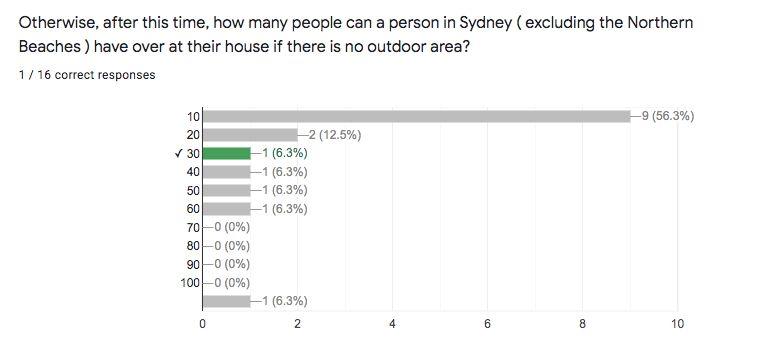
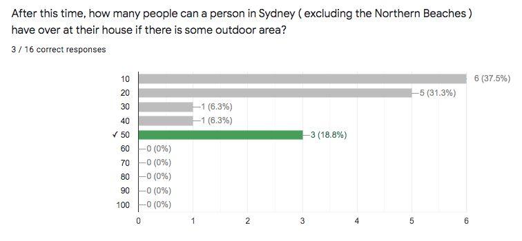
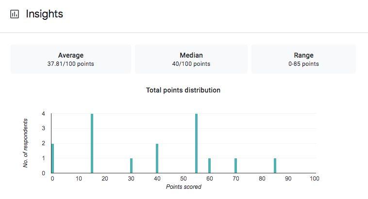
● MeasuresofCentralTendency ○ Averagewas37.81/100 ○ Medianwas40/100

● Botharebelow50%→mostfailedwiththeir awarenessofsocialisingregulations.

b.

● 32%selectedincorrectly ○ Thus thereisagapwhich Mona Talks Corona canfulfil.

c.

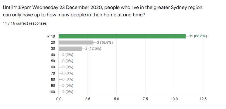
● Only6.3%werecorrect→apositivenoteisthat 68.8%underestimatedthisnumber.

● Mightsuggestatthistimeadolescentswere socialisingwithanumberofpeoplelowerthan therecommended→reducingtheprobabilityof transmission.

d.

● 18.8%werecorrect→ 81.2%underestimatedthe regulations ○ Potentiallydemonstrating(atthetimeof thesurvey)socialisationcouldhavebeen slightlyincreasedtosupportthemental wellbeingofourconsumers,another factortobeconsideredinconjunctionto maintainingphysicalhealth.

● Themostwantedanswerswereinregardstothe latestCOVID-19socialisingrestrictions.(86.6% )

○

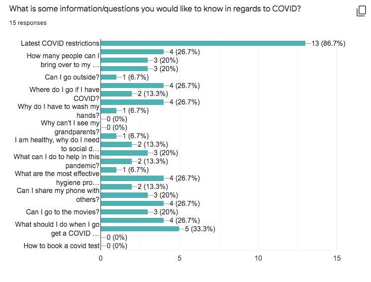
Followedby‘WhatshouldIdowhenI getaCOVIDtest?’at33.3%.Thisis extremelypertinentconsideringthata misunderstandingoftherequirementsor completedisregardiswhatledtothe NorthernBeachescluster.

LiteratureReview

Developingaresearchtopic

Communicatinginhealth:Findinganeffectiveandengagingwaytospreadimportanthealth informationaboutCOVID-19toadolescents.

Keywords

-Targetaudience:Adolescents

-Areoftenunawareofthesituation

-Communicationtypes:apps,advertisements,socialmedia,websites,chatbot.

-MentalhealthrelatingtoCOVID-19.

-Surveyingadolescents->seeingiftheyareawareofthechangingrulesandrestrictions regardingCOVID-19.

-Messagesaboutwhatiswrongorillegalincurrentsituations.

-Differentvaccinesandnewresearchtohelpwiththecoronavirus.

-Whichrestrictionsaremostrelevantforadolescents.

Flowchartofhowdifferentconceptsfitwithinthattopic

Reviewingotherliterature:

Leveraging media and health communication strategies to overcome the COVID-19 infodemic (https://link.springer.com/article/10.1057/s41271-020-00247-w)

● ThisarticlediscussedhowtheCOVID-19pandemicwasequallyan‘infodemic’

○ confusionthroughtherolesocialmediaplayedwithinformingadolescents→ contributingtothecreationofconspiracytheories.

○ Whatthisdictatesisthattheeffectivenessandvalidityoftheinformation communicatedisequallyimportant.

Effective health communication (https://www.ncbi.nlm.nih.gov/pmc/articles/PMC7180027/)

● Providesclearinstructionsonwhatmakeseffectivehealthcommunication+theimportance oflearningfromthispandemicsothattherewillbesystemsinplacefornexttime.

● Possiblyadisastertemplatecouldbeconsideredwherethefeaturesofthehealth communicationarespecifictoa‘newdisease’.

Reviewingexistingadvertisements:

● Germangovernmentcoronavirusadvertisement→ messagethatcouchpotatoesarethe ‘heroes’oftheCOVID-19pandemic.

○ effectiveasitishumorous,engagestheyouthandhelpsencouragepeopletoact responsibly.

Drawbackswithexistingsolutions:

Advertisements-Thissolutionmightnotbeaseffectiveforadolescentsparticularlybecausemanyof themdon’twatchliveterrestrialtelevisionandwatchnetflixorotherstreamingservices.

Sam-The‘chatbot’availablebytheDepartmentofhealthistailoredtothechallengesandconfusions experiencedbypredominantlyadults.

Researchquestion:

Thereisaseriousneedforcommunicatinginhealthduetothelackofplatformsavailablefor adolescentsandthusinfluencingtheirapproachtokeepingsafeandwellduringthepandemic.The primaryfocusofthisprojectwillbeontheproposedinnovativedesignforachatbottosolvethe struggleofcommunicatinghealthtothespecifiedconsumers.

Logbook

Atleast3designs,includingyourfinaldesignforasolutiontoyourproblem

Idea Positive Minus

TVseriessetinthefuturelooking backonourpresentwiththeaimto boostmoralesothatadolescentsare moreinclinedtofollowthehealth restrictionsthatarecommunicated tothem.

● Demonstrating therewillbea positiveoutcome tothispandemic hasthepossibility toincentiviseour targetmarketto contribute, knowingthisisa challengeour societycan collectively overcome.

● Alternativelythis videocanbe viewedinthelight thatwearesoclose tothesolution ○ A)why bother continuing tofollow thehealth recommen dations ○ B)our target marketof adolescent sdon’t believe their contributio nwas necessary.

Aninteractiveinstagrampagethat isregularlyupdatedwith communicatedhealthmessages directfromthedepartmentof health.

● Notcreatinganew platformwill ensurethatthenew servicewillbe easilyaccessibleto ourconsumers.

● Unfortunatelyour hashtagsand interactive activitieswouldbe subjecttothe trendsandwhims ofsocialmediato maintainthe

Interesting/Improvement

● Thisideawas inspiredbytheAd whichGermany created.Sincethe targetmarketis highlyengagedby TheOfficerelatedhumoura satiretvshow, featuringhumour aboutthe unprecedented timescould potentiallyfocus theattentionof adolescents towardsthe communicationof health.

● Wouldbea continuationofthe ‘#stayathome’ movementthatlost momentumduring thequarantine period.

Anautomatedchatbotsystem availableonpopularsocialmedia sites,tailoredtothequeriesof adolescentsduringCOVID-19. → Mona Talks Corona

● Responsesare immediateand constantlyupdated sotheyalignwith themostrecentand current communicated healthmessages.

● Candevelopa functioning prototypewiththe technologicalskill wehave.

Justificationofourselectedsolution

interestof adolescents.

○ Thiscould provetobe a significant struggle.

● Thelimitationsof thesoftwareitself ispresentinterms ofthequestions thatcanbeasked andanswered.The technologymight notbepreparedto answeralltypesof questions.

● Awayinwhich thisnegativehas beenimprovedin ourprototype developmenthas beenthroughthe useof abbreviationssoa widervarietyof inputswillbe accepted.

Mona Talks Corona effectivelywouldaddressthechallengeforadolescentskeepinguptodatewith allthehealthrestrictions,regulationsandrecommendations.Theidentifiedgapinthemarketisthe needtoaddressthehealthandwellbeingconcernsofourconsumers.Oursurveynoteswhichcanbe foundinthesectionTables,FiguresandAbbreviationsdemonstratestheconfusionandlackof knowledgeadolescentshaveinregardstothecurrenthealthclimate.Currentlythemethodsofhealth communicationarenotsuccessfulwithourmarket.

Thepositivefacetsofthisdesignarelistedinthepositivecolumnabove,withanadditionaldirect improvementwehaveemployedthatremovesthenegativewehadlisted.Outofallthedesignswe havediscussedingroupmeetingsthisnotonlywasdecidedthemostprobabletoworkinregardsto ouridentifiedproblembutthemostfeasibleforustocreatewiththeskillswehaveavailable.

Reflectionsofourprogressandmeetings

Meeting1-Wednesday11/11/203:30pm-4:00pm

Thiswasourfirstmeetingwithourmentorforthechallenge,PhilipPoronnik.Wediscussedsome possibleareaswecouldlookintoinourchosentopicarea.Philipletusknowaboutafewresources wecouldutilisewhenworkingwithhimandhealsosharedsomesourcestoaidwithourresearch. Duringthemeetingwediscussedthetargetaudience,leaningtowardsamoreyouthfulaudience,and westartedbrainstormingtheproblemwewouldliketocombat.

Throughouttheweek,weeachcarriedoutalittlebitmoreresearch,includinglawsregarding COVID-19safetyinworkplacesandinpublic,aswellasreadingafewarticlesandwatchingsomeof thevideosourcesweweresent.

Meeting2-Wednesday18/11/203:30pm-4:15pm

WefurtherdiscussedareasforustoresearchandmoreinterestingissuesrelatedtoCOVID-19that haven’talreadybeenoverlydiscussedthisyear.AftertalkingtoPhilipagain,wedevelopedaninterest inhowtheexcessiveuseofantibacterialproductssuchashandsanitiseranddisinfectantspraymay negativelyaffectourimmunesystems.Wewanttounderstandhowprolongedexposureto antibacterialsaffectsourmicrobialcommunitiesandwaystopreventthisaswellaswaysto communicatethepreventionmethods.Inourresearchdoc,wesetgoalstoachievebyournext meetingwithPhilip.Wediscussedlookingtothepasttoseehowpeopleovercamepastpandemics suchasbubonicplagueandSpanishflu.Further,welookedatwaystocreateamorepositiveproduct thatwouldmotivatepeopletomakegoodchange.

Meeting3-Wednesday02/12/203:30pm-4:00pm

Throughthetwoweeksbetweenmeetings,wehadlookedintopossibleproductstodevelopandwe’ve decidedtocreateachatbot.Thiswouldbeagoodmethodofcommunicationwithpeopleofdifferent backgrounds,particularlyregardinghealthandsafety.Betweenthissessionandournextinthree week’stime,weplantocontinueourresearchonchatbotsandwayswecancommunicatewithothers. Wearealsogoingtosurveyothersregardinguseexperienceandhowwecouldimproveonwhat alreadyexistsandcreatesomethinginnovative.

Meeting4-Wednesday23/12/203:30pm-4:00pm,onwards

Wemadeagoodstartonthechatbots,havingmadeafewprototypes.Wealsocreatedaposter, detailingafewstatisticsandthepurposeofourchatbot.Asurveyhadbeensentouttostudentsaged 13-18andwequizzedthemontheirknowledgeofcurrentCOVID-19restrictions.Usingourresults, wewereabletostartadataanalysis.Thedesignforthemascotofourchatbot,Mona,wasalso created.Wemadeagoodstartonourreportandwerewellontrackwiththeproject.

Wecontinuedtoworkonourprojectandconsultedwithourmentorforsomemoreadvice.We createdourslideandmadeseveralvariationsofthesameslidewithdifferentcolourstomatchthe template’scolourscheme.Whenwewerefinallyhappywithourslide,wemovedontofinalisingthe report.Thechatbotwascompletedandwecompiledalltheclipsofitworkingintoonevideo.

OURFUNCTIONINGPROTOTYPELINK:

https://youtu.be/uTAXS1nijfU

TheAmazonLexsoftwarewasusedtocodeandcreatethefunctioningchatbot.Afterattendingan Amazonenrichmentsessionduringschoolterm,thecodingskillsdevelopedwerethenabletobe directlyappliedtothecommunicationofhealthprojects.Withagrowingprevalenceoftechnologyin thelivesofyouth,creatingachatbotusingthissoftwarewasidealformeetingtheneedsofthetarget market.

Thefourmaincodingcomponentsofthechatbotwerethatof:

1.Intent-Havinganintentwasvitaltocreatingachatbot.Ithighlightsthetopicareaorgoalin whichtheusersqueriesaretoconcern.Akeyexampleofanintentwouldbe ‘bookatest’ whichexploresthequeriesaroundCOVID-19testingandassistsininitiatingbookingtest times.

2.Utterance-Astatementorquestionthatissaidbytheuserrelatestotheintent.I.eIwouldlike tobookacovidtestin{place}on{date}at{time}place.Thisthenhasembeddedslotsthatwill assisttheprograminaskingmorequestionstogathermoreinformationinregardstothe booking.

3.Slot-types-Arecreatedforeachintentandareusedtodefinehowdataintheslotis recognizedandhandled.Forthebookatestanalogyslot-typesincludedplaceslot(togain insightintotheuser’sstate),dateslot(forthepreferredtestingday)andtimeslot(forthetime ofdaypreferred).Undereachslottypestherearethepotentialoptionsthat theusermaysay.l i.e.date-monday,tuesdayetc.

4.Slots-defineanyinformationthebotcarriesoutinanintentandarelinkedtotheslot-type. Theyareembeddedintotheutterancesothatthebotisabletoaskmorequestionsandanswer thequerybasedontheresponsesfoundwithintheslot-type.I.e.Iwouldliketobookacovid teston{monday}(thedaywasalistedoptionunderthe slot-type)

Theprototypeisabletodirectlymeettheneedsofthetargetmarketwithoptionsforvoicetotextand texttovoice.Thisenablesclearcommunicationofrules,restrictionsandanswerstootherqueries answeredforallpeople. Additionally,multiplelanguageoptionsareavailablewithcodeavailablefor bothitalianandenglish(USandAUS)speakers.

ChallengesandFutureWork

● Infuture,ourchatbot Mona Talks Coronacouldbetailoredtoanswerquestionsonabroader scaleconcerningCOVID-19.Inthetransitionalperiod,betweennowandthenewnormalnew questionsandupdatedinformationwillbeadded. (i.ebacterialresistanceduetoourincreased hygienepractices)

● Potentialissuesthatmaycomeupintheproductionofourdesignwouldbethedifficultyin engineeringaneffectiveandeasy-to-usechatbotfeature.Wedesignedourownprototypeon AWSEducatebyAmazonanditsuserinterface isflawed.Infuturewemightwanttowork morefromscratch.

○ Wecanutiliseartificialintelligencetechnologytoanswerawiderrangeofquestions

Conclusion

Inconclusion,we’vediscoveredalackofknowledgeconcerningcurrentCOVID-19healthmessages andrestrictions.Inordertocombatthisissue,wehavecomeupwiththesolutionofachatbot,named Mona Talks Corona,toassisteverydayindividualsonCOVID-19-relatedinformationontheplatform oftheirroutinelyvisitedsocialmediasites.TheidenticalserviceacrosstheDepartmentofHealth websiteandsocialmediasiteswillmeanthatthesameinformationwillbeeasilyaccessibleto whereverourconsumersofadolescentswishtofindit.

References

AustralianGovernmentDepartmentofHealth.(2021). Coronavirus (COVID-19) current situation and case numbers. RetrievedfromJanuary4,2021,from https://www.health.gov.au/news/health-alerts/novel-coronavirus-2019-ncov-health-alert/coronavir us-covid-19-current-situation-and-case-numbers

AustraliaGovernmentDepartmentofHealth.(2021). Sam the chatbot. RetrievedNovember5,2021, fromhttps://headtohealth.gov.au/sam-the-chatbot

Fernando,G.(2020,November11). This German coronavirus ad is urging young people to be the heroes of 2020 - by staying at home on the couch. SBSNEWS.RetrievedonDecember28,2020, from https://www.sbs.com.au/news/this-german-coronavirus-ad-is-urging-young-people-to-be-the-heroe s-of-2020-by-staying-at-home-on-the-couch

Finset,A.(2020).Effectivehealthcommunication–akeyfactorinfightingtheCOVID-19pandemic. Elsevier Public Health Emergency Collection. RetrievedonNovember24,2021,from https://www.ncbi.nlm.nih.gov/pmc/articles/PMC7180027/

J,Andrews,L,Foulkes,&S,Blakemore.(2020).Vol.24,No.8 pg.(585-586).TrendsinCognitive Sciences.[PDF].RetrievedonJan7,2021.

Mheidy,N.,&Fares,J.(2020).Leveragingmediaandhealthcommunicationstrategiestoovercome theCOVID-19infodemic. Journal of Public Health Policy. RetrievedonNovember24,2021, fromhttps://link.springer.com/article/10.1057/s41271-020-00247-w

NSWGovernment.(2021). COVID-19 (Coronavirus). RetrievedfromJanuary2,2021,from https://www.health.nsw.gov.au/

NSWGovernment.(2021). Latest COVID-19 news and updates. RetrievedDecember31,2020,from https://www.nsw.gov.au/covid-19/latest-news-and-updates

Reuters.(2020,November16) 'Be lazy, save lives,' Germans urged in COVID video. [Videofile]. https://www.youtube.com/watch?v=FS1DDn2eklU

WorldHealthOrganisation.(2021). Coronavirus disease (COVID-19) pandemic. WorldHealth Organisation.RetrievedonDecember2,2021,from https://www.who.int/emergencies/diseases/novel-coronavirus-2019

Mona Talks Corona

BIOT UTURES 2021 MG018

J.Benedict, S. Jayatillake, V. Kim, L. Leonard, S. Witting

Academic Advisor: Ms Rachele Rugiero Mentor: Philip Poronnik