Sentiment
 Analysis Project with Python & Tensorflow

Analysis Project with Python & Tensorflow
The purpose of my analysis of this data is to answer the question, “Can I build a model to classify a review as either positive or negative with at least seventy percent accuracy?”
The goal of my analysis aligns with my research question. I would like to build a classification model that will yield at least seventy percent accuracy when classifying whether a text review is positive or negative.
I generated a recurrent neural network (RNN) in order to create optimum accuracy. The recurrent neural network yields more accurate classifications than a basic linear regression model would with this dataset because RNN models have hidden (dense) layers and also include optimization functions to minimize loss.
To start my exploratory data analysis, I printed the shape of my dataframe and found I had 3000 rows and 2 columns. Then, I used the .info command and value_counts() to find how many of each type of review (positive and negative) my data contained.
I checked for the presence of null values with the isnull().values.any() command to determine there were no null values contained in my dataset.
I knew it would be relevant to my analysis to make a column that contained the word count and also the character count for each row, so I used the split() and len() command to add those two columns to my dataframe. I sorted the dataframe by word total so that I could find the maximum word total contained within a single review in my dataset.
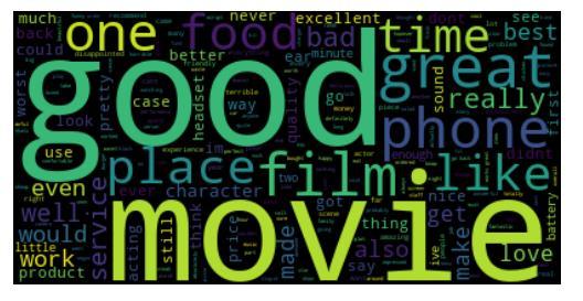
I created a wordcloud to get a good visual representation of what the most commonly used words were in this dataset. I wrote the code so that it would exclude common words (referred to as “stopwords”) that would not change the meaning of the reviews. Here is the output from the code I used to create my wordcloud:
Presence of unusual characters:
By printing my dataset, I was able to visually inspect the actual reviews and the text they contained. I saw that there was punctuation that should be removed to decrease my input vector size for the sake of preprocessing, but I did not see any emojis or non-English characters.
Vocabulary size:
In order to obtain my vocabulary size (count of unique words), I tokenized the ‘Reviews’ column and then printed the tokenizer.word_index. There were 5,402 unique words in the dataframe, but it is important to notice that this included stopwords.
Proposed word embedding length & statistifcal justification for the chosen maximum sequence length:
Since the sentence with the most words contains 71 words, my first thought was to use 71 as my proposed word embedding length. However, when I plotted a histogram of the word counts per sentence, I discovered that the distribution of the word counts is skewed right. (See image.)

Therefore, I decided to use 55 as a starting place for my word embedding length. I also knew I would be removing stopwords and lemmatizing after this, so my proposed maximum sequence length was likely to change after those preprocessing steps.
My goal throughout the tokenization process was to refine the data to produce the simplest, most efficient vectors for my machine learning model I wanted to create to perform sentiment analysis of this data. First, I changed all the letters in the “Reviews” column to lowercase letters, and then I removed the punctuation from all the reviews. I removed the stopwords, which reduced the overall unique wordcount from 5402 to 5279 Although it did not shorten the longest sentence, removing the stopwords did remove hundreds of words from the entire dataset (ProgrammingKnowledge, 2021).
After lowercasing the words and removing the punctuation and stopwords, I used the NLTK package to tokenize the words. I created two additional columns and added them to my dataframe to easily compare the original wordcounts to the reduced wordcounts after I removed the stopwords. I lemmatized the reviews column in a separate dataframe and did a reduced wordcount column so I could compare the lemmatized wordcounts with the wordcounts after removing the stopwords. I did not find a difference by visually inspecting, and I confirmed there was not any noticeable difference by creating a histogram of the lemmatized review columns and comparing it to the histogram of the reduced wordtotal column created by just removing the stopwords. I came to the conclusion that lemmatizing did not make a drastic difference and therefore did not do any further “normalization” of the Reviews column in the main dataframe df2.
Here is the code I used to prepare and tokenize my data:
##import relevant packages
import numpy as np
import pandas as pd
from pandas import Series, DataFrame
import nltk
import matplotlib.pyplot as plt
%matplotlib inline
import seaborn as sns
import warnings
warnings.filterwarnings('ignore')
import os
import datetime
import tensorflow.keras
from tensorflow.keras import Sequential
from nltk.tokenize import word_tokenize
from nltk.corpus import stopwords
import sklearn
##read in the data and concatinate the files (Sewell, 2016)
os.chdir('C:/Users/Ruth Wright/Downloads')
amazon = open('amazon_cells_labelled.txt', 'r').read()
imdb = open('imdb_labelled.txt', 'r').read()
yelp = open('yelp_labelled.txt', 'r').read()
amazon = amazon.split('\n')
imdb = imdb.split('\n')
yelp = yelp.split('\n')
amazon = amazon[:-1]
imdb = imdb[:-1]
yelp = yelp[:-1]
amazon = [x.split ('\t') for x in amazon]
imdb = [x.split ('\t') for x in imdb]
yelp = [x.split ('\t') for x in yelp]
t2data = []
for x in amazon:
t2data.append(x)
for x in imdb:
t2data.append(x)
for x in yelp:
t2data.append(x)
##Create dataframe with 2 columns
df2 = pd.DataFrame(t2data)
df2.columns = ["Reviews", "Positive_Score"]
df2.shape
##print dataframe
display (df2)
##Exploratory data analysis
df2.info()
##Get count of positive reviews and negative reviews
df2['Positive_Score'].value_counts()
##Add wordtotal and chartotal columns
df2['wordtotal'] = [len(x.split()) for x in df2['Reviews'].tolist()]
df2['chartotal'] = df2['Reviews'].apply(len)
df2
##Get max word total
dfsorted = df2.sort_values(by=['wordtotal'])
display (dfsorted)
##View distribution of word totals per sentence
df2.hist('wordtotal')
##Lowercase the review column
df2['Reviews'] = df2['Reviews'].str.lower()
df2
##Check the dataframe for null values
check_for_null = df2['Reviews'].isnull().values.any()
print (check_for_null)
##Import regular expression package to remove punctuation import string
import re from string import *
##Remove punctuation from the reviews column
f = re.compile(r'[^\w\s]+')
df2['Reviews'] = [f.sub('',x) for x in df2['Reviews'].tolist()]
df2
##Import relevant packages to create wordcloud from wordcloud import WordCloud, STOPWORDS, ImageColorGenerator from PIL import Image
##Create wordcloud from nltk.corpus import stopwords from nltk.tokenize import word_tokenize import nltk import matplotlib.pyplot as plt
from wordcloud import WordCloud, STOPWORDS, ImageColorGenerator from PIL import Image
stopwords = set(stopwords.words('english'))
stopwords.update(["br", "href"])
textt = " ".join(review for review in df2.Reviews)
wordcloud = WordCloud(stopwords=stopwords).generate(textt)
plt.imshow(wordcloud, interpolation='bilinear')
plt.axis("off")
plt.savefig('mywordcloud.png')
plt.show()
##Import packages and tokenize sentences import nltk
nltk.download('punkt')
import tensorflow.keras
from nltk.stem import PorterStemmer
porter=PorterStemmer()
from keras.layers import * from keras.preprocessing.text import Tokenizer from keras.preprocessing import sequence
my_data = []
for sentence in df2.Reviews:
my_data.append([word for word in word_tokenize(sentence)])
vocab_size = 50000
x = my_data
print('''\n''',x)
tokenizer=Tokenizer(num_words=vocab_size)
tokenizer.fit_on_texts(x)
x = tokenizer.texts_to_sequences(x)
print('''\n''',x)
##Print tokenized word index before removing stopwords print(tokenizer.word_index)
#Remmove stopwords from Reviews column
my_data = []
for sentence in df2.Reviews:
my_data.append([word for word in word_tokenize(sentence) if word not in stopwords])
vocab_size = 50000
x = my_data
print('''\n''',x)
tokenizer=Tokenizer(num_words=vocab_size)
tokenizer.fit_on_texts(x)
x = tokenizer.texts_to_sequences(x)
print('''\n''',x)
print(tokenizer.word_index)
##The next few blocks of code were written to compare the original wordcount to the reduced wordcounts after removing stopwords. ("Untokenize" the words and save as a new dataframe mydf2)
import re
mydf2 = pd.DataFrame(my_data)
pd.set_option('max_colwidth', 330)
print(mydf2)
##Create new column with "untokenized words" to add to the newly created dataframe mydf2
mydf2['Column A']=mydf2[mydf2.columns[0:]].apply( lambda x: ' '.join(x.dropna().astype(str)),
axis=1
)
mydf2.drop(mydf2.iloc[:,0:41], inplace=True, axis=1)
mydf2
##Add the two new columns with the reduced wordcount and character count to the main data frame df2
df2['Reduced Word Total']=[len(x.split()) for x in mydf2['Column A'].tolist()]
df2['Reduced Char Total']=mydf2['Column A'].apply(len)
df2.shape
df2.columns
df2
##Lemmatize the Reviews column
from nltk.stem import WordNetLemmatizer
lemmatizer = WordNetLemmatizer()
nltk.download('wordnet')
def lem (token_text):
text=[lemmatizer.lemmatize(word) for word in token_text]
return text
mydf2['Column A'].apply(lambda x: lem(x))
mydf2['Lemmatized_Words'] = [len(x.split()) for x in mydf2['Column A'].tolist()]
mydf2['Lemmatized Characters'] = mydf2['Column A'].apply(len)
mydf2
I chose tensorflow to build my model, and tensorflow only accepts input vectors that are the same length. Creating vectors that are all the same length requires padding. Padding is a function that fills in zeros as values to create vectors that are a set length. For instance, if the chosen length for the vectors is 30 tokens and a vector only includes 6 values, the padding function fills in 24 zeros to make the vector 30 tokens in length. The pad_sequence() function accepts an argument, ‘padding’, which can be set so the zeros are filled in at the beginning of the function or at the end of the function (padding = ‘post’). I chose to fill in the zeros at the end of the text sequence so I used the ‘post’ padding option (StatsWire, 2021).
Because I chose a maximum sequence length of 30, and there were many sentences that contained more than 30 tokens, I also had to use the “truncating” argument. I set the “truncating” argument to ‘post’ so that the values were eliminated from the end of a text sequence if it contained more than 30 tokens.
The following is a screenshot of a single padded sequence:
There are only two categories of sentiment. The score of zero indicates a negative review and a score of one indicates a positive review. Since this is a binary dataset, I used the ‘sigmoid’ activation function in the last dense layer of my neural network.
There are several steps I implemented to prepare this data for sentiment analysis. I created a dataframe with the data and then changed all the letters to lowercase. I also removed the punctuation and all the stopwords. I tokenized and lemmatized the data and then vectorized it. I padded and truncated the vectors so that they could be used as input vectors in my neural network. I used the train_test_split function to split the data into training and testing sets, and I decided to use ninety percent of the data for training which left ten percent for the testing set. I also set the validation level at 10% when I built my model.
Here is a screenshot of the output of my TensorFlow model summary:

There are a total of five hidden layers in my model plus an output layer. The first layer is an embedding layer, the next layer is a spatial dropout layer, then the LSTM layer, followed by another dropout layer. (The dropout layers reduce overfitting in the final model.) The last dense layer utilizes the ‘sigmoid’ activation layer because it fits well with binary models. The output layer includes the ‘binary_crossentropy’ loss minimizer, and the ‘adam’ optimizer.
There are a total of eleven parameters.
Choice of hyperparameters:
Activation function: I chose the sigmoid activation function because I generated a binary classification model.
Number of nodes per layer: Choosing the best number of nodes is an experimental process, but choosing a lower number of nodes reduces the processing time for training the model. I chose to use 128 in my LSTM layer because it was efficient.
Loss function: I chose to use the ‘binary_crossentropy’ loss function because it is well-suited to reduce the loss in binary classification models such as mine.
Optimizer: The purpose of optimizers in neural networks is to adjust the weights and learning rates to efficiently reduce the loss in the model. The ‘adam’ optimizer is very effective because it can handle sparse gradients with on problems with lots of “noise.”(Brownlee, 2021)
Stopping criteria: Since this was a relatively small dataset that only included 3000 rows, I decided to set the epochs to twenty. This means that the model would iterate through all the data 20 times and then stop. I could have also set the patience level to 2 or 3 to make the model stop training once it reached a “plateau,” but since I decided to run the model through 20 epochs and inspect the accuracy of the results before I included a patience argument. I was able to obtain a high level of accuracy without invoking the patience argument.
Evaluation metric: I chose to use the ‘accuracy’ evaluation metric for a few reasons. The most important reason I chose to use the ‘accuracy’ metric is that it is easy to understand. The accuracy output is a decimal which translates to the percentage of times the classification model correctly identified the class. The second reason is that the accuracy metric is ideal for binary datasets that have approximately a fifty-fifty split of the scores, and this dataset had exactly a 50/50 split.
Summary of epochs and batch size:
The number of epochs I chose determines how many times the model iterates through the entire dataset. Since this is a small amount of data, relatively speaking, I chose to do 20 epochs. For larger datasets, the number of epochs may need to be much larger in order to get a sufficiently high percentage of accuracy. Also, for larger datasets, the analyst may need to set a batch size that breaks the dataset into “chunks” and processes each “chunk” as it iterates through the entire dataset. Here is a screenshot of the final epoch of my model:
The time stamp shows that the model iterated through my entire dataset twenty times in only 7 seconds.
Here is a screenshot of the line graph depicting the accuracy and loss of the function as its training process took place:

The blue line represents the accuracy of the training data, while the orange represents the accuracy of the validation set of data. The screenshot of the output of the last epoch shows that the accuracy of the
trained model is over eighty percent, and the validation accuracy is over seventy percent, which is sufficient for the purpose of this project. The gap between the blue line and the orange line indicates a small percentage of overfitting, but since the gap is mostly consistent, the slight overfitting is not a huge issue.
Predictive Accuracy:
The predictive accuracy of this model is much better than blindly guessing. A guess would yield a fifty percent rate of accuracy, and this model boasts an accuracy of around eighty percent. (We see that it is exactly 81.89% according to the model output from the last epoch because of the nature of the “accuracy” metric.)
Code to save trained network:
Here is the code I used to save the trained network within my RNN: ##Save model sentiment_analysis = model.save
RNN justification:
This RNN classification model is ideal for this dataset because it ran very efficiently and smoothly. The running time for the training process was less than 10 seconds. Not only did it train quickly, but the accuracy of the model was great as it reached over eighty percent accuracy. A final thought about the effectiveness of this model is that overfitting was prevented due to the dropout layers I invoked
Recommendation:
I recommend that this model be used for business stakeholders wanting to efficiently determine whether their customer feedback reviews are mostly positive or negative. The management of the customer satisfaction department of a business could use this analysis to determine whether their efforts are meeting customer needs, etc.
Sources:
Brownlee, Jason. (2021, January 13). Gentle Introduction to the Adam Optimization Algorithm for Deep Learning. Machine Learning Mastery. https://machinelearningmastery.com/adamoptimization-algorithm-for-deeplearning/#:~:text=Adam%20is%20a%20replacement%20optimization,sparse%20gradients%20o n%20noisy%20problems.
“TensorFlow Tutorial 18 TensorFlow Padding.” YouTube, uploaded by StatsWire, May 28, 2021 https://www.youtube.com/watch?v=9ieVC_ABDNQ
“Python NLTK Tutorial 2 Removing stop words using NLTK.” YouTube, uploaded by ProgrammingKnowledge, March 21, 2021. https://www.youtube.com/watch?v=LLl3bQXhhzI