Data Cleaning & PCA in R

Data Cleaning in R

& Principle

Component Analysis (PCA)

Data Dictionary & Summary

The raw data set in the file ‘churn_raw_data.csv’ contains 10,000 anonymized records of customer demographics, churn status and purchasing behavior from a well-known telecommunications company and also includes each customer’s answers to a customer satisfaction survey. There are 65 variables in the cleaned, treated data set. There were 52 in the original data set, but I added 14 more variables through my cleaning process. The following is a chart that describes the data types and lists an example of each variable.

This is a description chart of the original dataset.

discrete. Provided as a placeholder to indicate order of the data as it imported into R Studio.

CaseOrder

Customer_id

Interaction character

discrete. Provided as a placeholder to indicate the

order of the raw data set.

Qualitative, nominal. Provided as a unique expression to identify each client.

Qualitative, nominal. Unique expression for labelling interactions with clients.

K191035

2b451d12-6c2b-4cea-a295ba1d6bced078

City character Qualitative, nominal. Client’s city where they live. Del Mar

County character

Qualitative, nominal. Client’s county of residence. San Diego

Zip integer Quantitative, discrete. Client’s postal code. 92014

Lat numeric

Lng numeric

Population integer

Quantitative, discrete. The latitude of client’s GPS coordinates of their residence.

Quantitative, discrete. The longitude of the client’s GPS coordinates of their residence.

Quantitative, discrete. The reported population within 1 mile radius of client’s residence per US Census Bureau.

32.96687

-117.2479

13863

Area character

Qualitative, nominal Categorization of the client’s residential address per US Census Bureau.

Urban

TimeZone character

Job character

Qualitative, nominal Time zone of the client’s residence. America/Chicago

Qualitative, nominal. Invoiced person’s stated vocation Solicitor

Children integer Quantitative, discrete. Client’s stated number of children in household.

4

Age integer Quantitative, discrete. Client’s stated age. 50

Education character

Employment character

Income numeric

Marital character

Gender character

Churn character

Qualitative, ordinal. Client’s stated highest degree earned Doctorate Degree

Qualitative, nominal. The client’s stated employment status. Student

Quantitative, discrete. The client’s stated annual income. 18342.12

Qualitative, nominal. The client’s stated marital status. Married

Qualitative, nominal. The client’s response to gender inquiry as nonbinary, male, or female

Qualitative, ordinal Yes/No answer indicates if client discontinued service within last month.

Female

No Outage_sec_perweek numeric

Quantitative, discrete. The mean number of seconds weekly a system outage occurred in the client’s close geographical area

11.835113

Email integer

integer Quantitative, discrete. The instances that the client had to contact technical support

16

3 Yearly_equip_failure integer

Quantitative, discrete. Customer’s times that equipment failed in the last year that needed replacements or resetting.

3

Techie character

Contract character

Qualitative, ordinal. Yes/No answer indicates if client originally considered themselves tech savvy.

Qualitative, ordinal. Customer’s category of contract term monthly, annual, biannual.

Yes

Month-to-month

Port_modem character

Tablet character

InternetService character

Phone character

Multiple character

OnlineSecurity character

OnlineBackup character

Qualitative, nominal. Yes/No answer indicates if they possess a portable modem.

Qualitative, nominal. Yes/No answer indicates if customer possesses a tablet device.

Yes

Yes

Qualitative, nominal. Client’s choice of internet service. DSL

Qualitative, ordinal. Yes/No answer indicates if client purchases a phone service.

Qualitative, ordinal. Yes/No answer indicates if they purchase multiple phone lines.

Qualitative, ordinal. Yes/No answer indicates if they purchased an online security add-on.

Qualitative, ordinal. Yes/No

answer indicates if the client purchased an online backup addon.

No

No

Yes

Yes

DeviceProtection character

TechSupport character

StreamingTV character

StreamingMovies character

PaperlessBilling character

PaymentMethod character

Tenure numeric

MonthlyCharge numeric

Qualitative, ordinal. Yes/No answer indicates if the client purchased a device protection add-on.

Qualitative, ordinal. Yes/No answer indicates if the client purchased a technical support add-on.

Qualitative, ordinal. Yes/No answer indicates if the client purchases streaming television.

Qualitative, ordinal. Yes/No answer indicates if the client purchases streaming movies.

Qualitative, nominal. Yes/No answer indicates if the client opts for electronic billing.

Yes

Yes

Yes

No

No

Qualitative, nominal. Client’s preferred payment method. Electronic Check

Quantitative, continuous. Client’s total time with this company in months.

Quantitative, discrete. The average charge invoiced to this client per month.

2.415992

230.62376

Bandwidth_GB_Year numeric

Quantitative, discrete. The average gigabytes of data utilized by this client in the past 12 months.

Item1 integer Quantitative, discrete. The client’s rating of the value of timely responses with scores 1-8. (1 is most important, 8 is least important.)

Item2 integer Quantitative, discrete. The client’s rating of the value of timely fixes with scores 1-8. (1 is most important, 8 is least important. Same scoring for Item1 through Item8.)

Item3 integer Quantitative, discrete. The client’s rating of the value of timely replacements with scores18. (1 is most important, 8 is least important. Same scoring for Item1 through Item8.)

Item4 integer Quantitative, discrete. The client’s rating of the value of reliability with scores 1-8. (Same scoring for Item1 through Item8.)

Item5 integer Quantitative, discrete. The client’s rating of the value of options with scores 1-8. (Same scoring for Item1 through Item8.)

Item6 integer Quantitative, discrete. The client’s rating of the value of respectful responses with ratings 1-8. (Same scoring for Item1 through Item8.)

Item7 integer Quantitative, discrete. The client’s rating of the value of courteous exchanges with scores 1-8. (Same scoring for Item1 through Item8.)

Item8 integer Quantitative, discrete. The client’s rating of the importance of evidence of active listening with scores 1-8. (Same scoring for Item1 through Item8.)

1259.4155

2

1

1

2

4

2

1

3

This is a description chart of the 13 additional variables that I created throughout my treatment plan.

Quantitative, discrete. The StreamingMovies values reexpressed as ordered numbers.

Plan to detect data anomalies:

2

My plan for identifying data anomalies includes measures to detect possible duplicate values, missing values, and outliers. I will also re-express the ordinal categorical variables as numerical to prepare the dataset for PCA. The steps to detect the anomalies are as follows:

Step 1: I will begin by importing the churn_raw_data file into the R studio environment using the dropdown menu under “File” and choosing the “Import Dataset” option, then choosing the “From text (base)…”

Step 2: Next, I will use the read.csv function included within the dplyr package to read the csv file as a data frame and give the data frame the name “treated_churn_data”. Then, I can display the structure of the data frame using a str() command. Displaying the structure will allow me to observe its dimensions the number of variables and observations. The structure command will also allow me to examine the data types of each variable.

Step 3: I will determine if there are any duplicated rows by using the duplicated() function on the data frame.

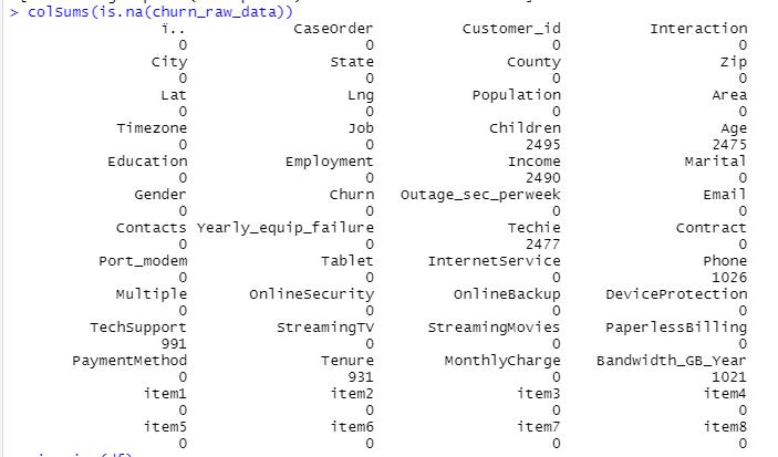
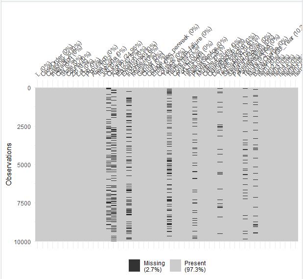
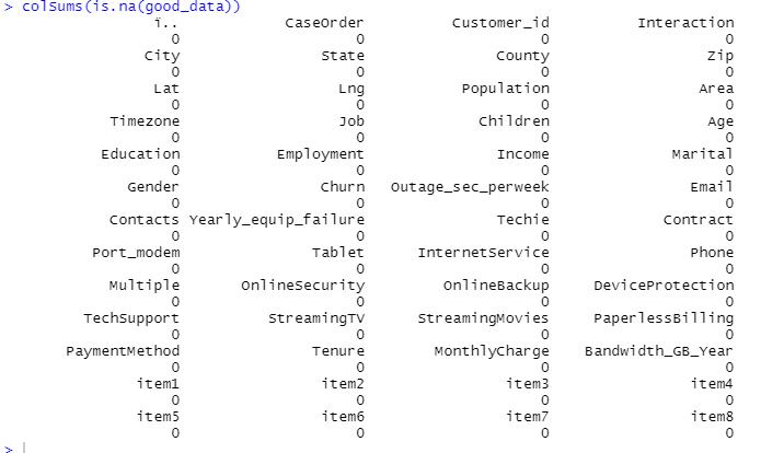
Step 4: I will determine exactly how many missing values exist within each variable by pairing the colSums function with the is.na function for this data frame. This function will provide the count of missing values for every variable in the data set. I will also create a visualization of the missingness of the data by using the vis_miss function from the visdat package. This visualization also identifies the percent of missing values for each variable, along with the percent of missingness for the entire data frame.

Step 5: The next step will be to treat the missing values, because I cannot proceed to detecting outliers without the possibility of the missing values interfering with my detection of outliers. The best treatment method for missing values will need to be determined after carefully considering the percent of missingness, type of data and its context in this dataset, which I will further explain in part D of this task.

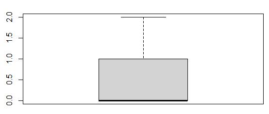
Step 6: Next, I will determine if outliers exist among the quantitative variables, excluding the variables that serve as labels for the order or contain data about geographic locations such as the GPS coordinates, zip code and population variables. (The geographic and population information was obtained from third-party sources according to the provided data dictionary, and so is assumed to be correct.) The process I will use to determine if outliers exist within the quantitative variables is to create a boxplot for each variable using the boxplot function from the ggplot2 package, and then check the boxplot to see if any values exist outside the “whiskers” or

edges of the boxplot. I will use the boxplot()$out command to discover the values and quantity of outliers if they exist within that variable.

I will calculate the z-score in addition to creating boxplots for certain variables that warrant further inspection within the context of this dataset. I will be using the scale() function to calculate the z-score, and then I will create a variable for the z-score and add it to the data frame. This will enable me to write a query to discover the exact value and amount of the outliers that exist within that variable according to their z-score.

Step 7: Finally, I will re-express the ordinal qualitative variables as numerical variables to prepare them for Principle Component Analysis. I will use the revalue() function of the plyr package to perform the conversion from categorical to numeric.

Justification of cleaning plan:

Because the data set includes 10,000 rows with 52 columns, using the duplicated () function that is included in R studio is much more efficient and accurate than manually examining the data for duplicates. For the same reasons, determining missing values should be conducted by using the colSums and is.na functions, which detects missing values for the entire data frame in mere seconds. The additional step of creating visualizations of the missing values through visdat is simple and is well worth the small effort it requires, because the graphical display indicates what percentage of values are missing. The visualization can also give clues as to whether there is any type of relationship among the missing values if there are “groupings” within the display.

Outliers are only present in quantitative variables, so only those type of variables need to be examined. Boxplots are ideal to identify outliers because they determine and clearly display the central tendency of the data set regardless of the distribution, unlike z-scores, which can be affected by skewness. Boxplots are also a better choice than histograms, because histograms can be misleading when outliers are close to the other values. Within a boxplot, outliers are very easy to distinguish because they are the values that appear on the outside of the “whiskers”, and running the boxplot()$out command efficiently displays the number and value of outliers (Larose & Larose, 2019).

Certain variables may contain outliers that are effectively described by using their z-scores within the context of this dataset. The reason for this is that in some cases there are significantly less records that are considered outliers using the z-score method than using the boxplot method. In the cases in which removing the outliers from the boxplot method would result in too many rows being removed, I will explore the use of the z-score method as a viable option.

The reason I plan to re-express the ordinal categorical variables as numerical variables is to prepare the dataset for the Principle Component Analysis. PCA is only able to calculate quantitative values, so re-expressing the categorical variables in a numeric format could possibly result in greater dimensionality reduction when the PCA is performed.

Justification for using R:

The R programming language is ideal for cleaning this data set because I can very easily create powerful visualizations using simply imported packages. For instance, the visdat package allows me to create a visualization of the missing values within my data set, and also includes the exact percentage of missing values within each variable in addition to the entire data set with only one short line of code. Creating the same chart in Python would require more steps

Another justification for using R versus Python is that the initial download of R contains the scale () function that calculates the z-score with one line of code (which can be useful when detecting outliers), while Python requires several steps to calculate z-scores, including importing packages, to perform the same function. Also, performing Multivariate Imputation by Chained Equations (MICE) is simple in R because there is a MICE package that conveniently contains all the functions needed to execute logical regression and predictive mean matching with just a few lines of code.

The availability of the ggplot2 package is exclusive to R, which is another reason I chose to use the R programming language. The ggplot2 package for R is ideal for creating boxplots because they can be created with only one line of code, and customization of the boxplots is available and simple to execute as well.

In addition to the aforementioned reasons to choose the R programming language for this project, performing Principle Component Analysis in R is far simpler than using Python. Using R reduces the number of lines of code by about half, since it automatically extracts all the PCs and applies the PCA to the normalized dataset.

Cleaning Results Summary:

To briefly summarize my results from implementing my plan for detecting data anomalies, I found no duplicates, but I did detect missing values in 8 of the variables, as well as outliers in 15 of the variables. In addition, I also re-expressed 12 ordinal categorical variables as numeric.

Missing Values Summary:

The visualization I created by calling the colSums function shows that there were a significant number of missing values in the Children, Age, Income, Techie, Phone, TechSupport, Tenure, and Bandwidth_GB_Year variables. I have included a screenshot of the missingness chart, which also gives the percentage of missingness for each variable. This is a helpful feature when

trying to quickly determine if enough records are missing to warrant imputation or removal. (Removal is only a viable option if 5% or less of the records are missing in a variable.)

Screenshot of summary of missing values in each of the variables:

Missingness Chart:

Outliers Summary

I found outliers in the following quantitative variables: Children, Income, Outage_sec_perweek, Email, Contacts, Yearly_equip_failure, MonthlyCharge, Item1, Item2, Item3, Item4, Item5, Item6, Item7, and Item8.

The boxplots and description of the outliers for each quantitative variable I explored are shown below:

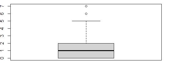
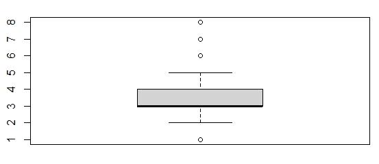
Boxplot of Children

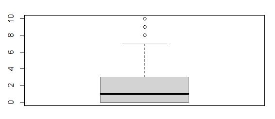
The boxplot for Children depicts values of 8, 9, and 10 as outliers. There are 420 outliers in this variable.

Boxplot of Age

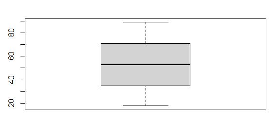
The Age variable did not contain any outliers, and does not require further treatment.

Boxplot of Income

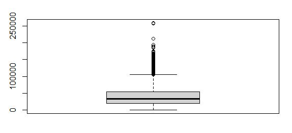
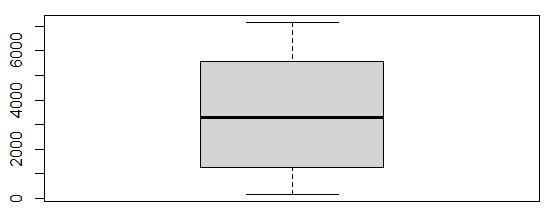
The Income boxplot showed that any income above $ 104867.50 was an outlier, and there were 344 records in that category Since that is a relatively large amount of outliers, I decided to explore using the z-score method. When I calculated the z-score, I found that only 153 entries had a z-score higher than 3, and the lowest income in that category was $126236.20. I decided to use the z-score method for this outlier because it would be more reasonable to treat 144 values versus risking the loss of valuable data by using the boxplot method.

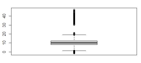
From the boxplot, I can see that outliers exist above and below the boxplot. There are 539 outliers. However, the z-scores indicate that there are 491 records with a z-score higher than 3, but none with a z-score lower than -3. It is also significant to observe that there is a small range of values within the Outages variable (observations range from -1.348571 to 47.04928) Since the z-score outliers do not represent the lower outliers depicted in the boxplot, it is more relevant to use the boxplot to describe the amount of outliers for this variable. This variable contains 539 outliers.

Boxplot of Outage_sec_perweek

Boxplot of Email

Within the Email variable, I found outliers below and above the normal range of values. I used the boxplot()$out command to find the number of emails that were outside the normal range, and there were only 38 entries that belonged in the category of outlier. The normal range is indicated by the boxplot to be between 4 and 20 emails sent.

Boxplot of Contacts

The boxplot indicated values of 6 and 7 as outliers. There were only 8 entries in the outlier range for the Contacts variable.

Boxplot of Yearly_equip_failure

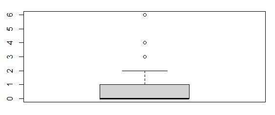
The boxplot depicted values of 3, 4, and 6 as outliers. There were 93 outliers in total in the Yearly_equip_failure variable.

Boxplot Tenure

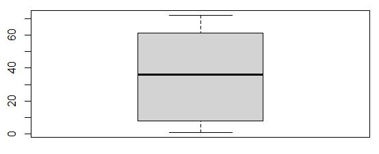
No outliers exist in the Tenure variable, so no further treatment is needed.

Boxplot of MonthlyCharge

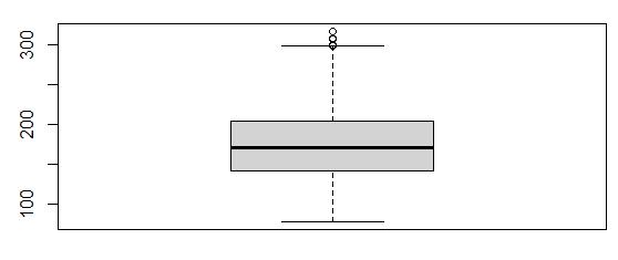
The outliers for the MonthlyCharge variable were any charges above $298.00. There are only 5 clients in the data set that incurred a charge in the outlier range, with the maximum value being about $316.00

Boxplot of Bandwidth_GB_Year

No outliers exist in the Bandwidth_GB_Year variable, so no further treatment is needed.

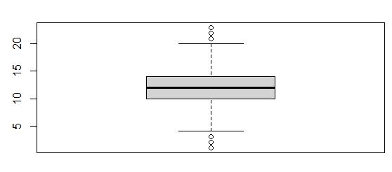
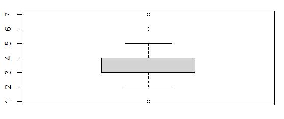
Boxplot of Item1

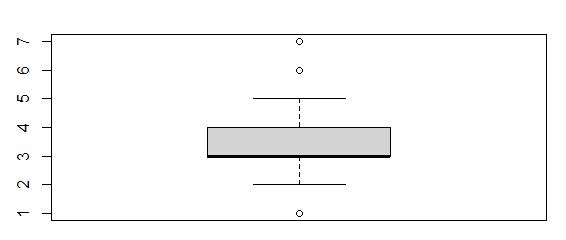
From the boxplot we can see values of 1, 6, and 7 are considered outliers. There are 442 outliers.

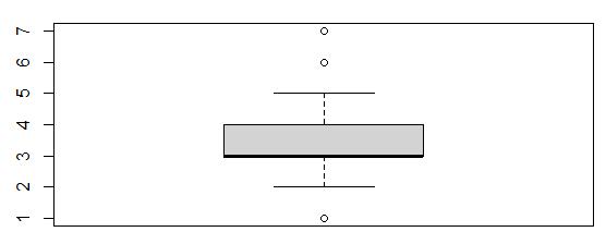
Boxplot of Item2

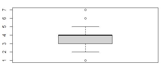
This boxplot showed that values of 1, 6, and 7 were outliers. There were 445 outliers in the Item2 variable.

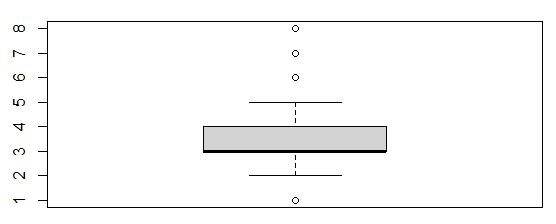
Boxplot of Item3

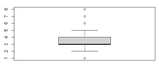
The Item3 boxplot showed that values of 1, 6, 7, and 8 were outliers. There were 418 outliers in Item3.

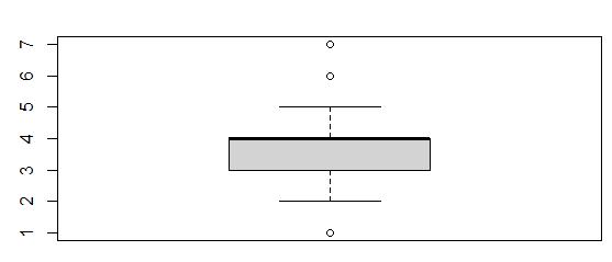
Boxplot of Item4

This boxplot showed that values of 1, 6, and 7 were outliers. There were 433 outliers in Item4.

Boxplot of Item5

This boxplot showed that values of 1, 6, and 7 were outliers. There were 422 outliers in Item5.

Boxplot of Item6

This boxplot showed that values of 1, 6, 7, and 8 were outliers. There were 413 outliers in Item6.

Boxplot of Item7

This boxplot showed values of 1, 6, and 7 were outliers. There were 455 outliers in Item7.

Boxplot of Item8

This boxplot showed values of 1, 6, 7, and 8 were outliers. There were 426 outliers in Item8.

Treatment of Missing Values:

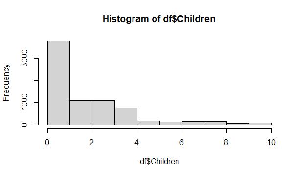
After examining the dataset, I concluded that none of the data is consecutive data, so I could not use backward and forward fill imputation. Also, I could not reasonably assume a constant value for any of the missing values, so specific value imputation was not an option. When I explored the use of univariate implementation by imputing the median of the Children variable (a quantitative variable) in place of the missing values, I noticed that the distribution of the cleaned data was noticeably different from the distribution of the raw data in the Children variable as shown in the illustration below.

Raw Data Histogram:

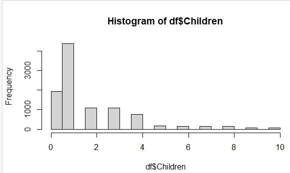
Histogram after univariate imputation, using the median value for imputation.

This prompted me to explore the MICE method for imputation (DataExplained !, March 2020) I decided to use Multivariate Imputation by Chained Equations (MICE) to impute data in place of the missing values because the distribution of the data from each variable was much closer to the original distribution than when I tried univariate imputation. Another benefit to choosing this method was that I could perform the imputation on the entire dataset versus one variable at a time.

Because there are many choices of methods within MICE, I had to determine which method would work for the type of data I was treating. When the variables were numerical, I passed the pmm method (predictive mean modeling) to the MICE function, and when the variables were categorical, I passed it the logical regression method.

I have included some modeling of the effects on the distribution of the data after using MICE to treat the missing values of the quantitative variables in the dataset in the histograms below:

Raw data from the Children variable, which includes 2,495 missing values:

Cleaned data from the Children variable using MICE imputation (predictive mean matching) with no missing values:

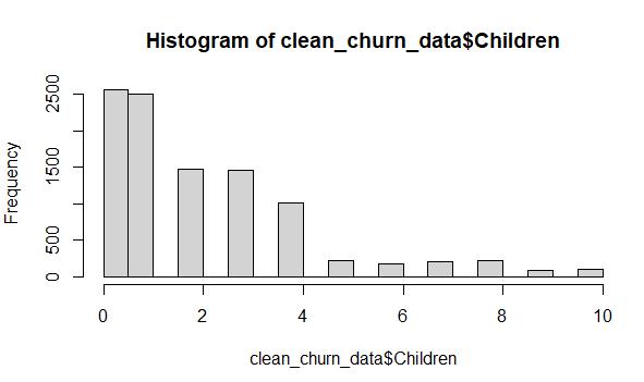
The distribution of the two datasets is very similar. The exception is that there are fewer instances of the “0” value in the cleaned data histogram and more instances of the “1” value, but the effect is negligible since those are the lowest values in the data set.

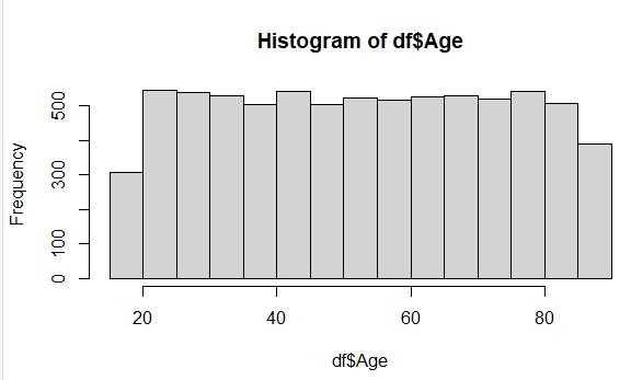
Raw data from the Age variable, which includes 2,475 missing values:

Cleaned data from Age variable after using MICE imputation (predictive mean matching):

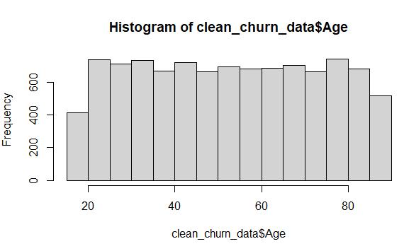
Once again, the distribution of the raw and cleaned data sets are nearly identical after using MICE imputation, even though there are more data points represented in the cleaned data set.

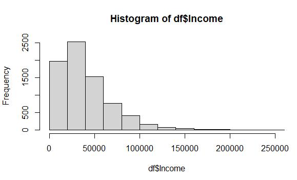
Raw data from the Income variable, which includes 2,490 missing values:

Cleaned data from the Income variable using MICE imputation (predictive mean matching):

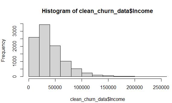
The histogram of the cleaned Income data shows that the distribution was preserved through the MICE imputation method. The data is still skewed to the right, and the ratios of the bars are almost identical to the original depiction of the raw data set.

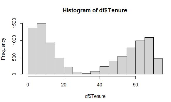
Raw data from the Tenure variable, which includes 931 missing values:

Cleaned data from the Tenure variable using MICE:

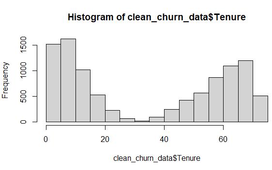
The original histogram of the raw Tenure data depicts a bimodal distribution, which is a difficult distribution to treat using univariate imputation methods. This is an ideal situation for using MICE, and the results that in the cleaned data histogram clearly illustrate that the bi-modal distribution stayed intact throughout the process.

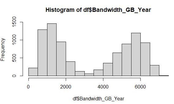
Raw data from the Bandwidth_GB_Year variable, which includes 1021 missing values:

Cleaned data from the Bandwidth_GB_Year variable after MICE imputation:

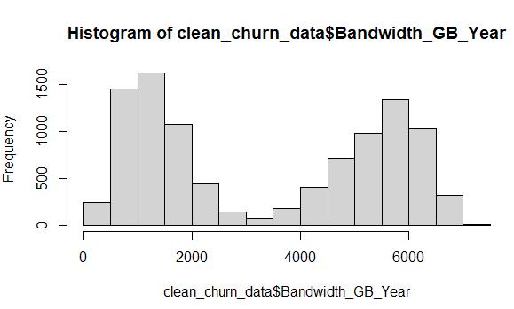
The Bandwidth variable is another prime candidate for MICE imputation, due to its bimodal distribution. After employing the MICE method, the cleaned data histogram depicts the same shape as the original raw data.

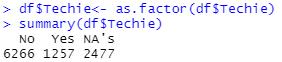
The MICE method also works especially well for categorical data, although the variables must first be converted into factors using the as.factor() function. (DataExplained!, March 2020). For these categorical variables, the MICE package performs logistic regression to more closely predict what value should be imputed in place of the missing values than simply imputing the mode for each missing values. The method worked extremely well for the Techie variable, as shown in the screenshots below. Notice that the percentage(distribution) of “No” and “Yes” answers is the same in the raw data and cleaned data. (The raw data contains about 83% “No” answers and 17% “Yes” answers, excluding the missing values. After MICE is performed, the “No” answers still account for approximately 83% of the “No” answers and 17% of the “Yes” answers.)

Summary of raw data from Techie variable:

Summary of cleaned data from Techie variable:

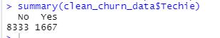
The summary screenshots depict that 2,477 missing values were imputed, yet the distribution stayed very close to what it was in the raw data.

The remaining two categorical variables, Phone and TechSupport, can also be successfully treated with MICE as illustrated below:

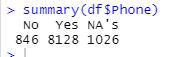
The MICE imputation method replaced 1,026 missing values in the Phone variable, with the distribution remaining very close to the original. Roughly 9% of the answers are “No” in both the raw and the cleaned data, with approximately 11% of the answers as “Yes” both before and after the cleaning method was implemented.

Summary of raw data from Phone variable:

Summary of cleaned data from Phone variable:

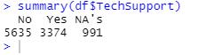
The final categorical variable, TechSupport, was successfully treated with the MICE method as well. About 63% of the answers are “No” in both summaries, with about 37% of the responses as “Yes” in both the raw and cleaned data sets.

Summary of raw data from TechSupport variable:

Summary of cleaned data from TechSupport variable:

To verify that all of the missing values were treated, I passed the colSums(is.na()) function my cleaned data set. The screenshot below shows that there are no more missing values in this data set.

Treatment of Outliers

For the Children variable, I found 420 outliers, and all of them were above the normal range. Since the outliers were values that were reasonable (8, 9, and 10), I decided to retain these records. I considered omitting 420 rows as too risky because it could result in the loss of valuable data for later analysis.

The Income variable boxplot showed 344 rows that contained outliers (values above $ 104867.50), all of which were above the normal range. I considered that to be too many rows to safely remove, but I believed that the outlier incomes were significantly impacting the central tendency of the this data set. Therefore, I decided to use the z-score method to find values that had z-scores higher than 3, and discovered there were only 144 records with z-scores above 3. So, I decided to exclude the z-score outliers by first saving them in a separate data frame

“out.incomedf” using a which() query, and then removed them from the main data set. The boxplots below show the “before” and “after” of the treatment method.

Income Boxplot before exclusion method applied:

Income Boxplot after exclusion method applied:

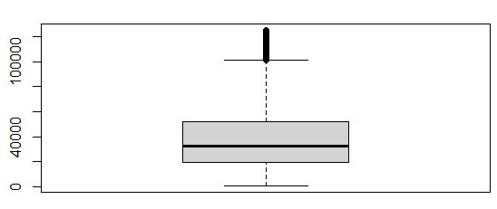
The lower boxplot only 276 outliers, and the maximum value is around $124,000.00. Therefore, the dataset no longer contains the extreme outliers that would interfere with effective analysis.

The Outage_sec_perweek variable did contain variables, but I decided to retain the values for two reasons. Firstly, the source of the data is derived from actual outages in the client’s neighborhood. Secondly, all of the values in this column were within a relatively small range of 48 seconds, so I did not consider the outliers to be extreme.

The Email variable also contained outliers. The boxplot showed there were 38 variables outside of the normal range any that were below 4, and any above 20 I decided to exclude these outlier records from the dataset since the amount of records was very small relative to the entire dataset. I wrote a query to store the outliers in a data frame titled “out.emaildf” and then removed them from the main data frame. The boxplots below illustrate the effectiveness of this treatment method.

The Email Boxplot before the exclusion method was applied:

The Email boxplot after the exclusion method was applied:

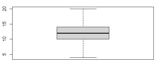
The results boxplot shows that there are no longer outliers in the Email variable.

The Contacts column contained 8 outliers according to its boxplot. I considered the outliers to be extreme as they were values of 6 and 7, and the median value was 1. Since there were only 8, I decided to exclude the outliers by placing them in a separate data frame, “out.contactsdf.” The, I ran a -which() query to drop them from the good_data set (Larose & Larose, 2019) The following boxplots verify the exclusion of all outliers from the Contacts variable.

The Contacts boxplot before exclusion of outliers:

The Contacts boxplot after exclusion of outliers:

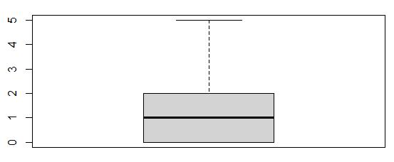
The boxplots illustrate that the outliers are no longer present in the Contacts variable.

The Yearly_equip_failure column contained 93 outliers, which were values of 3, 4, and 6. I decided to exclude rows with these values from the data set because they were extremely far away from the median value of 0, and there were a relatively small number of records containing outliers in relation to the entire dataset. I have illustrated the effectiveness of this treatment in the boxplots below.

The Yearly_equip_failure boxplot before exclusion:

The Yearly_equip_failure boxplot after exclusion of outliers:

The second boxplot is free from the outlier values of 3, 4, and 6. It only contains values from 0 through 2.

The Monthly Charge variable contained 5 outliers, all of them above the normal range, but they were relatively close to the normal range. The maximum value in the dataset was $315.88, and the upper boundary for normal is $298. I decided to retain the outliers since there are only a few and the margin by which they are outside the normal range is small.

There were outliers in the Item1, Item2, Item3, Item4, Item5, Item6, Item7, and Item8 variables. I listed the specific number of outliers for each of these in section D1. To summarize, the number of outliers for each of these categories is between 413 and 455, but the ranges for each dataset are relatively small. (They each contain a range of 8 variables). Since removing or excluding that many rows would jeopardize the integrity of the dataset, and the range of responses is relatively small, I decided to retain the outliers in these variables.

Re-expression of Categorical Variables:

I expressed the following categorical variables as numeric variables by creating a new variable with the same name followed by “.numeric”: Education, Churn, Techie, Contract, Phone, Multiple, OnlineSecurity, OnlineBackup, DeviceProtection, TechSupport, StreamingTV, and StreamingMovies. For example, the numeric re-expression of Education is named “education.numeric.”

For Education, I used the following numbers to represent each education level when I created the new variable as a numerical re-expression:

0 = “No Schooling, 8 = “Nursery School to 8th Grade” , 9 = “9th Grade to 12th Grade, No Diploma”, 11 = “GED or Alternative Credential”, 12 = “Regular High School Diploma”, 13 = “Some College, less than one year”, 14 = “Some College, 1 or More Years, No Degree”, 14 = “Professional Degree”, 15 = “Associate’s Degree”, 16 = “Bachelor’s Degree”, 18 = “Master’s Degree”, and 20 = “Doctorate Degree.” Each education level roughly corresponds to the number of years of education

For the Churn re-expression variable, I assigned “Yes” the value of 1 and “No” the value of 2, since “No” is better in this context. (“Yes” means that the client has left the company in the past month.)

For the Techie re-expression variable, I assigned “Yes” as 2 and “No” as 1, because being technologically inclined requires more practice and skills than a “No” response.

For the Contract re-expression variable, I assigned values based on the number of months of the 3 different contract types. 1 = “month-to-month”, 12 = “one year”, and 24 = “two year”.

For the Phone, Multiple, OnlineSecurity, OnlineBackup, DeviceProtection, TechSupport, StreamingTV, and StreamingMovies re-expression variables, I assigned “Yes” with 2 and “No” with 1, since each of those columns indicate that a client purchased that service if there is a “Yes.” Assigning a higher value to the “Yes” responses makes sense because the context of this dataset is to identify and keep highly profitable customers.

Justification for using the MICE imputation method:

The two available options to treat missing data are either removing the records with missing values or using some time of imputation. Removal of missing data points is only a reliable option when the total amount of missing values is less than 5% of the entire data set, since removal negatively affects the sample size of the dataset.

The MICE method I employed for treating the missing values is only as accurate as the amount and accuracy of the data it receives. It is an advanced method for predicting what data is missing, as it finds hidden “patterns” among the missing data values and predicts what the best match would be. The more data it contains to work with, the more accurate the prediction is. In other words, it is limited by the percent of missingness and available “pattern” among the known data values. Also, it is wise to consider that any imputation method used is just a prediction

The treatment of outliers is more complex. If you are able to prove that the outlier is a factual error, then removal is the best option. If the outliers are legitimate values but are distorting the distribution of the dataset too much, you can use the exclusion method instead. This means that you first save the outlier values to a separate data frame and drop them from the main dataset. (The exclusion method was the method I used to clean this dataset, instead of removal.)

Retaining the outliers within the dataset is another option when you know that the data is legitimate, but you must recognize that the outliers exist. The final option is to impute a value such as the median in place of the outliers, but there is the risk of distorting the distribution of the dataset.

Suggested future analysis:

My research question, “Is there a higher churn rate among customers whose average number of seconds per week of system outage is higher than the mean number of seconds per week of system outage?” involves the Churn variable and the Outage_sec_perweek variable. The Churn variable was an ordinal categorical variable, so I re-expressed it as the numeric variable churn_numeric. This re-expression simplifies the coding for finding the churn percentage to answer my research question.

The Outage_sec_perweek variable did not contain missing values, but it did contain outliers. However, the range of values was relatively small (48 seconds total), so I decided to retain the outliers. Therefore, the results of any analysis performed on this dataset to answer my research question would not be negatively affected by the limitations of my data cleaning process.

Principle Component Analysis (PCA):

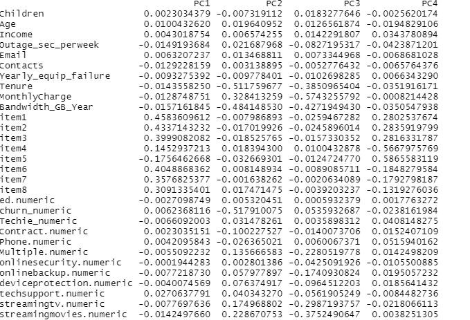
The principle component analysis I conducted produced 30 PC loadings, since I had 30 variables, which are:

Children, Age, Income, Outage_sec_perweek, Email, Contacts, Yearly_equip_failure, Tenure, MonthlyCharge, Bandwidth_GB_Year, item1, item2, item3, item4, item5, item6, item7, item8, ed.numeric, churn_numeric, Techie_numeric, Contract.numeric, Phone.numeric, Multiple.numeric, Onlinebackup.numeric, Onlinesecurity.numeric, deviceprotection.numeric, techsupport.numeric, streamingtv.numeric, streamingmovies.numeric.

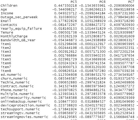
After analysis, I found there are 7 principle components in my dataset. I have listed them here:

Principle Component 1 through Principle Component 4:

Principle Component 5 through Principle Component 7:

Process Summary for PCA:

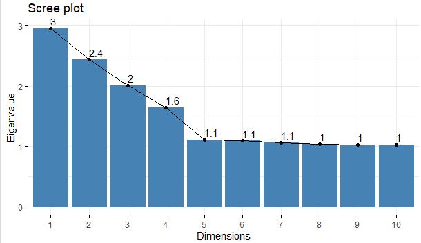
To identify the principle components of my dataset, I utilized the RStudio environment and loaded the factoextra package. I also loaded the visdat library to enable use of the fviz_eig() function. I passed the prcomp function all rows and the column numbers of the thirty numerical variables from my cleaned dataset, and saved the result as a data frame. The prcomp function calculated 30 principle components, so I created a scree plot of the eigenvalues to determine which principle components I should keep using the fviz_eig() function. This is the scree plot I created:

I used the “Kaiser Rule” to determine that I should only consider the first six principle components, because those are the only PCs that had an eigenvalue greater than one. As you can see from the scree plot, only 7 of the loadings have an Eigen value more than 1.

Benefits of using PCA:

The benefit of using the principle component analysis is that it significantly reduces the dimensionality of this dataset. The thirty numeric variables can be “grouped” into just 7 principle components for analysis without risking the integrity of the data. Reducing dimensionality would help any type of analyses run much more efficiently, and the data would also require much less space to store. To summarize, using these principle components would save time and space, which potentially translates to more profit.