Issuu

Sandy soil constraints in south east South Australia: a guide to their diagnosis and treatment Melissa Fraser, PIRSA May 2021

Funded by: The Murraylands and Riverland Landscape Board and Limestone Coast Landscape Board through funding from the Australian Government’s National Landcare Program.

Key messages: • Most sandy soils have multiple constraints that vary with individual

sand types and their location in the landscape. • It is vital to look below the surface to diagnose the presence, extent

and severity of different constraints. • Treatment strategies should address the range of constraints present

to get the best results.

Background There are more than 2.2 M ha of sandy soils in the Murray Mallee and South East regions of South Australia that are prone to develop poor fertility. Despite improvements in crop management and agronomy, there is often a large gap between the potential grain yield that could be achieved, based on rainfall, and the actual yields of crops grown on sandy soils1.

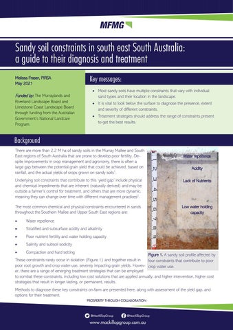
Water repellence

Acidity

Underlying soil constraints that contribute to this ‘yield gap’ include physical and chemical impediments that are inherent (naturally derived) and may be outside a farmer’s control for treatment, and others that are more dynamic, meaning they can change over time with different management practices2.

Lack of Nutrients

The most common chemical and physical constraints encountered in sands throughout the Southern Mallee and Upper South East regions are:

Low water holding capacity

•

Water repellence

•

Stratified and subsurface acidity and alkalinity

•

Poor nutrient fertility and water holding capacity

•

Salinity and subsoil sodicity

•

Compaction and hard setting

Figure 1. A sandy soil profile affected by These constraints rarely occur in isolation (Figure 1) and together result in four constraints that contribute to poor poor root growth and crop water-use, severely impacting grain yields. Howev- crop water use. er, there are a range of emerging treatment strategies that can be employed to combat these constraints, including low cost solutions that are applied annually, and higher intervention, higher cost strategies that result in longer lasting, or permanent, results. Methods to diagnose these key constraints on-farm are presented here, along with assessment of the yield gap, and options for their treatment.

Contents Diagnosing sandy soil constraints 1.1 Water repellence 1.2 pH 1.3 Nutrient status and soil texture 1.4 Salinity and sodicity 1.5 Compaction and hard setting 1.6 The yield gap

Treating sandy soil constraints 4 5 6 7 9 11

2.1 Water repellence 2.2 Acidity and alkalinity 2.3 Nutrient fertility 2.4 Water holding capacity 2.5 Salinity and sodicity 2.6 Compaction and hard setting 2.7 Management and agronomy post amelioration 2.8 References and resource links

13 13 14 15 15 15 18 19

1. Diagnosing sandy soil constraints As the presence and extent of constraints varies across sandy dune swale landscapes, the aim of diagnosis is to identify: Where the different constraints exist in the paddock topography  How do the constraints differ between the dunes, mid-slope and flats? The depth of layers affected by different constraints  At what depths do different constraints start and stop? The severity of the constraint/s present  Is the constraint mild, moderate or severe?

• • •

To reliably achieve this aim, paddocks should first be separated into strategic diagnostic zones for soil assessments, otherwise important issues can be missed or diluted. Tips to identify diagnostic zones for sampling: • Aerial imagery (such as Google Earth) can provide an indication of soil type and topographical zones, providing a good base layer map to separate out dunes and swales (Figure 2a). • Soil proximal sensors, such as electromagnetic induction (EMI), identify changes in soil properties (Figure 2b) and often show a strong correlation to crop and pasture production. At a cost of $15 to $20/ha, EMI maps are a worthy investment. They require thorough ground-truthing after collection to confirm the cause of variation (soil type, moisture content, salts). • Plant production measures such as above ground green biomass as shown by normalised difference vegetation index (NDVI; Figure 2c) and grain yield maps can both identify the boundaries of different production zones. Maps derived in a legume phase (beans, lentils or chickpeas) are useful for detecting acidity issues, as these crops are particularly sensitive to low pH. The number of diagnostic zones generated (usually 3 to 5) will depend on the variation within the paddock and its size; zones will typically separate the dunes, mid-slope and heavier flats. Once these maps have been created, field-based diagnosis of the soils’ physical and chemical fertility can begin. Tools to include in an on-farm diagnosis kit: •

Shovel, post hole digger or front end loader

•

Hand trowel

•

3 x buckets

•

Rain water

•

Push probe or penetrometer

•

Medicine/eye dropper (from the chemist)

•

pH indicator dye (e.g. Manutec)

•

Zip-lock plastic bags and marker pen

•

Camera and stop watch (mobile phone)

•

Tape measure or ruler 2

Figure 2a. Aerial photograph of a paddock with typical dune swale topography in south east South Australia3.

Zone 1 Clay loam

Zone 2 Sand over shallow clay Zone 3 Deep sand

Figure 2b. Map showing differences in soil electrical conductivity, collected using an electromagnetic induction sensor (EM38); ground truthing showed three distinct soil types in the paddock, reflected by the conductivity zones.

Figure 2c. Normalised difference vegetation index4 (NDVI) of a winter cereal crop, showing lower above ground green biomass in October in Zone 3.

Figure 2d. Soil pHCa map, generated using a grid-sampling technique, whereby 8 samples are collected within each 2 ha grid, analysed and reported. Soil pH shows a correaltion with the soil types as identified by EM38 (2b).

1.1 Water repellence Water repellence is a common problem on sandy soils, with waxes from decayed organic material coating grains to make them hydrophobic, impeding water infiltration and affecting seedling germination early in the season. The presence and severity of water repellence can be determined annually by conducting a water droplet penetration test, which assesses the time it takes for demineralised water to infiltrate the soil (Figure 3). This test is best conducted in summer and autumn and must be performed on dry soil. Sample from zones into which you intend to sow this year, either on-row, edgerow or mid-row.

Diagnosis In paddock observations: • Within each diagnostic zone, carefully scrape off the surface organic matter and 2-3mm topsoil layer in an area free of standing stubble, weeds and plant roots, to expose a level surface for testing. Using an eye dropper, carefully place three consistently large droplets of demineralised water (or clean rainwater) on the surface, dropped from the same height (Figure 3). Record the time it takes to infiltrate and determine the degree of repellency (see Table 1). Consider repeating this at 20, 40, 60, 80 and 100 mm depths to gauge repellency through the sowing layer. Repeat in at least 2 other locations within each diagnostic zone to confirm. Collecting samples: • Scrape off the surface organic matter and 2-3mm topsoil layer. Collect a sample from the top 50 mm and place in bucket #1. Collect a second sample from the 50-100 mm layer and place in bucket #2. Ensure samples are representative of the whole depth layer. • Repeat in 3 to 5 sample locations within each zone, combining samples from each depth in the relevant bucket; mix well. Collect combined soil in labelled sample bags. • Repeat for each diagnostic zone within the paddock. • Spread and level a layer of each soil on a labelled plastic tray (takeaway or similar) and place in a warm spot until fully dry. Assess the degree of repellency, following the water droplet penetration procedure as described above. •

Table 1. Severity of water repellence as indicated by the water droplet penetration test5. Non-repellent

Mild

Moderate Severe

Water infiltrates dry soil in 5 seconds or less.

Water takes longer than 5 seconds, but less than 60 seconds to infiltrate. Water takes 60 to 240 seconds to infiltrate. Water takes more than 4 minutes to infiltrate.

Figure 3. Soil is severely repellent if a droplet of water remains on the surface for longer than 4 minutes.

At the Lab: The Molarity of Ethanol Droplet (MED) test is used to objectively assess the severity of repellence. Follow the ‘collecting samples’ procedure described above and send to an accredited laboratory for MED analysis. An agronomist can assist with sample submission forms. 4

1.2 pH pH is a measure of the activity of hydrogen (H+) and hydroxyl (OH-) ions in the soil solution6, indicating acidic (low pH), neutral, or alkaline (high pH) conditions. It’s important to know the pH through the soil profile as the availability and form of macro- and micronutrients can be affected, resulting in plant deficiencies or toxicities where acidity and alkalinity prevail7. As with water repellence and compaction, surface and subsurface pH is usually non-uniform across whole paddocks, often changing between soil types or topographical positions (see Figures 2a to 2d), so strategic soil sampling methods are required to accurately detect pH variability (see pH variation in Figure 4). Acidity can have a severe impact on the productivity of crops and pastures by releasing toxic amounts of aluminium into the soil solution, stunting root growth and limiting nutrient availability and biological activity. Stratified acid bands are becoming increasingly common under no-till cropping, even in soils that were previously thought not to be prone to the development of acidity. Alkalinity is caused by the accumulation of carbonates and bicarbonates of calcium and/or sodium, impacting phosphorus and trace element availability. Soils dominated with calcium carbonate will have a pHw up to 8.2, whereas soils with a pH >8.5 indicate the accumulation of sodium carbonate and bicarbonate, creating toxicities to the plant and also often leading to the physical deterioration of soil structure (see section 1.4). Soil pH is commonly measured in a 1:5 solution of soil to water (pHW), or soil to calcium chloride (pHCa). As pH can be affected by soil moisture status and seasonal conditions, it is recommended to measure pHCa, particularly when the soil is acidic. This test is offered by all commercial laboratories and enables test results from different seasons to be more reliably compared. The pHCa is often 0.5 to 1 unit lower than pHW. To achieve optimum plant growth, the soil pHCa should be maintained between 5.8 and 7.3 in the top 10 cm, and above 4.8 in the subsurface (below 10 cm). pH indicator dye can be used to quickly and cheaply determine whether high or low pH is contributing to poor plant growth, but as the indicator solution can deteriorate over time and the observations are visual (subjective), care should be taken with interpreting results.

Diagnosis In paddock observations: • Within each diagnostic zone, dig 3 to 5 holes to 40 cm, creating a flat vertical soil profile face. • Apply pH indicator liquid dye down the profile and then apply the powder and let the colour develop (Figure 4). Alternatively, you can use a Dig Stick soil probe (spurr probe) to remove an intact soil core and apply the same procedure to assess the change in pH. • Once the colour reaction is complete, use the diagnostic colour card to determine the pH down the profile. Any acid layers will be visible as bright green or yellow colours. The pH measured with this dye is equivalent to pHW, so the ideal pH is between 6 and 8 on the card (Table 2). • Use a tape measure to identify the positions of any pH changes and take a photo, including the tape measure for future reference. At the Lab: If pH variability has been identified using indicator dye, additional soil sampling and more accurate laboratory pH measurement and other analyses are recommended: • Within each diagnostic zone, collect 10 to 15 cores, combining the soil from each relevant layer depth in a clearly labelled bucket. • Depending on the position of the alkaline and acid layers in the profile, soil depths for sampling might include: 05, 5-10, 10-20 and possibly 20-30 cm. If acidity is more common in the 5-15 cm layer, then depths of 0-5, 5-15 and 15-25 cm are more appropriate.

•

Thoroughly mix the samples for each layer depth for each zone and bag a sub-sample; send to an accredited labo atory for pH analysis, organic carbon % and a soil texture assessment (this information is needed to calculate a lime rate if the soil is acidic). Aluminium (measured in CaCl2) is also warranted, along with electrical conductivity and exchangeable cations if the soil is alkaline (see section 1.4).

Table 2. Severity of acidity and alkalinity, as determined using pH indicator dye and a colour chart, which is roughly equivalent to the pH in water.

Alkalinity

Acidity

Rating

Severe Moderate Mild Neutral - ideal Mild Moderate Severe

>9.0 8.5 8 6.5 to 7.5 6 5.5 <5

Alternatively, precision soil sampling approaches, such as grid-based (Figure 2d) or on-the-go Veris® pH mapping can provide more detailed data on the variability in surface pH and possible stratification. These maps can be used to generate variable rate lime prescriptions.

Figure 4. Example soil pit face with pH indicator dye applied. An alkaline surface layer can be seen (purple), overlying acidic soil (bright green) below 3cm.

1.3 Nutrient status and soil texture Nutrient deficiencies and subsoil toxicities are common in sandy soils and can change rapidly within paddocks. Monitoring soil nutrient fertility in the top 10 cm of soil provides an indication of whether nutrients and organic carbon are being maintained or mined in your system over time. All commercial and accredited laboratories measure nitrogen, phosphorus, potassium, sulphur, exchangeable cations and organic carbon in their basic soil test suites. Soil texture determinations, such as particle size (% sand, silt and clay), provide an indication of the soils’ ability to retain and supply soil water (water holding capacity). Interpretation guidelines are usually included with soil test results but to derive the most benefit, recommendations should be tailored to the individual soil types within each diagnostic zone; an agronomist can assist with these interpretations and corrective strategies. In-season tissue testing can also provide a useful indicator of nutrient availability to the plant, rather than total nutrient concentration in your soil. Assessing the chemistry and texture in the subsoil is also warranted, particularly where clayey B horizons are present within the rooting zone, and also when considering deep ripping operations, so as to avoid disturbing areas where subsoil toxicities exist. The common subsoil constraints include extremes in pH (both acidity and alkalinity; section 1.2), salinity and sodicity (section 1.4) and toxic concentrations of chloride and boron. Various testing packages are offered at commercial laboratories to assess these constraints.

Diagnosis • •

Collect soil samples from each diagnostic zone to assess soil nutrient status and soil texture; for crops and pastures collect samples from the 0 to 10 cm layer. Subsoils are commonly sampled in 10 to 30, 30 to 60 and 60 to 90 cm depth increments, however, horizon boundaries should not be crossed, so the increments selected should reflect soil horizon characteristics. 6

• •

Within each diagnostic zone, collect >15 cores, combining the soil from each relevant layer depth in a clearly labelled bucket. Thoroughly mix the samples for each layer depth for each zone and bag a sub-sample; send to an accredited laboratory for full chemical and nutrient analysis along with a texture assessment, such as MIR particle size to determine the proportions of sand, silt and clay. A ‘fit for purpose’ guide to soil sampling can be found here, and tips for specifically diagnosing subsoil constraints can be found here. Precision approaches to soil fertility assessment can also be conducted using grid sampling methods.

1.4 Salinity and sodicity Salinity refers to the accumulation of water-soluble salts in the soil, having a direct impact on plant growth, whereas sodicity relates to the proportion of exchangeable sodium on the cation-exchange complex, which when elevated can lead to clay dispersion in the soil6, having an indirect impact on crop growth through the loss of soil structure. Salinity reduces a plant’s ability to extract water from the soil and can cause toxicities from specific ions8. Soluble salts are present most commonly as sodium and chloride, but also of potassium, calcium and magnesium as sulphates or carbonates6. Salinity is becoming more prevalent in both irrigated and dryland sandy soils across the Murraylands, Riverland and Limestone Coast. Saline seeps are an emerging problem that have rapidly increased in presence, size and severity across sandy soil landscapes over the last decade. Their emergence is due to a combination of topographical, seasonal and farming system factors that lead to waterlogging, scalding and salinisation, often in the most productive zones in the paddock9. Learn more about Mallee Seeps in this video and in resources here and here.

The severity of salinity is determined by measuring the electrical conductivity of a soil:water suspension, commonly in a 1:5 ratio by weight, reported in deciSiemens/metre (dS/m). Handheld conductivity meters are quick and easy to use, following the instructions for use and regular calibration but the most accurate results are obtained by sending soil samples to an accredited laboratory. High exchangeable sodium (sodicity) facilitates the dispersion of clay particles that can block soil pores, impeding infiltration and drainage, resulting in boggy, crusty and pugged soils. They commonly set very hard when they are dry, much like cement. As sodicity affects clay soils, rather than sands, it is more likely to be detected in subsoil layers where the clay content increases. It’s important to know if subsoil sodicity is present prior to ripping, delving or clay spreading to enable optimum amelioration. Sodicity is determined by measuring the amount of exchangeable sodium in the soil in comparison to the other cations (calcium, magnesium and potassium); it is reported as the exchangeable sodium percentage, or ESP, on a soil test.

Diagnosis In paddock observations that may indicate the presence of salinity8: • Crop symptoms – reduced yield and burnt leaf tips and margins • Die back of trees and sensitive plant species • Patches of bare soil • Salt crusts when dry and waterlogging after rainfall • Areas of prolific summer weeds In paddock observations that may indicate the presence of sodicity: • Sandy soils with very low infiltration rate • Very dense clay-ey B horizons 7

Cloudy puddles and surface water following rainfall Boggy patches of soil that set very hard when dry High susceptibility to gully and tunnel erosion Sodicity can be assessed visually by conducting a spontaneous dispersion test:  Collect dry soil aggregates from each sampling layer depth in each diagnostic zone.  Gently place the aggregates in a dish of demineralised water.  Observe the degree of cloudiness around the aggregates at 10, 30 and 120 minutes. If the water becomes cloudy with fine clay particles, you can suspect the presence of sodium in the soil (Figure 5).

• • • •

Figure 5. Degrees of dispersion for soils that are non-sodic (left) to severely sodic (right)10. At the lab: • Collect soil as per the instructions in 1.3 and send to an accredited lab to measure EC, exchangeable cations and the exchangeable sodium percentage. • Determine the soil salinity rating and likely impact on plant response (Table 3) and the severity of sodicity (Table 4). Table 3. Soil salinity ratings determined by measuring electrical conductivity (EC 1:5) for different soil textures (clay percent); from Hazelton and Murphy6. Clay % 10 to 20 20 to 40 40 to 60 60 to 80 Salinity rating Effect on plant growth EC1:5 (dS/m) Non-saline

<0.07

<0.09

<0.12

<0.15

Mild

0.07 – 0.15

0.09 – 0.19

0.12 – 0.24

0.15 – 0.30

Moderately sensitive crops affected

Moderate

0.15 – 0.34

0.19 – 0.45

0.24 – 0.56

0.30 – 0.70

Moderately tolerant crops affected

Severe

0.34 – 0.63

0.45 – 0.76

0.56 – 0.96

0.70 – 1.18

Tolerant crops affected

Very severe

0.63 – 0.93

0.76 – 1.21

0.96 – 1.53

1.18 – 1.87

Very tolerant crops affected

>0.93

>1.21

>1.53

>1.87

Extreme

No effect

Usually too saline for crop growth

Table 4. Soil sodicity rating, ESP and degree of spontaneous dispersion 6 and 10. Exchangeable sodium Sodicity rating Soil dispersion test percentage Non-sodic 0-6 No dispersion after 24 hours. Mild

6 – 10

A milky halo (dispersion) evident after 24 hours.

Moderate

10 – 15

Dispersion evident after several hours.

Severe

>15

Dispersion evident in less than 30 minutes. Soil aggregates completely disperse. 8

1.5 Compaction and hard setting Plant roots need to easily penetrate soil in order to rapidly grow. Their ability to do this is impeded when the soil is compacted (high bulk density caused by machinery compression or livestock trampling) and/or when the soil strength is too high. Soil strength is a measure of the soil resistance to failure when a force is applied and is very dependent on the clay and soil moisture content. Soil strength often increases as the profile dries, including in sands where oxides of iron and manganese are present, as these are prone to forming cemented layers (hard setting).

Diagnosis Soil pit observations • Hard and compacted layers can sometimes be visually observed in sands by digging a pit in each diagnostic zone and looking and feeling for changes in soil structure. Compacted layers or hardpans often have a distinct massive or blocky appearance when dry and may have fractures through them where plant roots are preferentially growing. • Crop vigour and the depth and pattern of root growth can also be useful indicators of physical issues; excavate the soil carefully under crop rows to explore the rooting pattern, including under wheel ruts. • In late spring and summer, compacted layers may be wetter than the soil above it, indicating that plant roots have been unable to penetrate this layer to extract deep soil moisture reserves. Soil strength Simple assessments of soil strength can be made using a push probe: • Make a push probe by fixing a handle onto a 600 mm long x 12 mm wide high carbon steel rod; sharpen the tip into a 20-22mm long, smooth cone and etch 100 mm depth increments along the shank of the probe. • Insert the probe by hand into wet soil. Use the depth increments on the shank to help identify the depth where hard layers start and finish. Such a probe will require 12 kg of down pressure per MPa of soil strength. This means a very dense soil will require up to 40 kg of downward pressure when inserting the probe (equivalent to a soil strength of up to 3.5 MPa; Table 5). More reliable and objective assessments of soil strength can be achieved using an instrumented cone penetrometer (Figure 6), which accurately measures the force required to insert a standard sized cone (12.83 mm) into the soil and is reported in either kiloPascals (KPa) or megaPascals (MPa)11. • Insert the penetrometer into the soil using steady pressure to achieve a constant speed of 3 cm per second. Note the change in penetration resistance (PR) for different depths in the soil. Repeat multiple times in the surrounding area to gauge the average PR and record the severity for each 10 cm layer (Table 5). Repeat in 3 to 5 locations in each diagnostic zone.

Tips for measurement: • • •

Push probes and penetrometers should be used when the soil profile is fully and uniformly wet to avoid misleading effects caused by lack of moisture alone; this is best achieved in mid-winter. Download the Soil Water App to assess soil moisture conditions. If the soil is dry, wet up an area in each diagnostic zone using a large bucket or tub with 2mm holes drilled in the bottom. Fix a porous cloth to the base (chux or similar) to assist even wetting across the surface area. Backfill around the outside edge of the bucket using soil to ensure downward infiltration, before filling with water and allowing to drain. The following day carefully dig down to depth on one edge to confirm the profile wetting is deep enough and collect 3 to 5 penetration measurements on the wet-up area.

• • •

Compare paddock readings to un-trafficked areas, such as along fence lines or in native vegetation. Avoid wheel tracks, headlands, gate ways and other high traffic areas; alternatively, measure these areas separately to gauge machinery impact on soil compaction. Penetrometers are unsuitable for use in soils with more than 10 to 15% gravel12.

Table 5. Effect of penetration resistance on root growth6 and 11 Penetration Degree of consoliResistance Rating Effect on root growth dation (MPa) Nil <0.50 Loose Not affected. Root growth on some cereal Mild 0.50 – 1.50 Medium plants may be restricted. Moderate

1.50 – 2.50

Dense

Severe

2.50 – 3.50

Very dense

Extreme

>3.50

Extremely dense

Compaction developing. Root growth on most plants starts to Root growth restricted to existing pores and planes of weakness. Significant compaction present. Root growth virtually ceases.

Figure 6. An example of an instrumented cone penetrometer, sourced here.

At the lab: Bulk density (BD) refers to the mass of soil in a given volume, commonly expressed in g/cm3, and primarily affects the soils porosity and strength11. BD measurements are useful for confirming compacted layers and are also needed for converting soil nutrient concentrations from mg/kg to kg/ha (e.g. nitrogen). Bulk density is measured by collecting an intact soil sample using a steel ring of a known volume (Figure 7). The retained soil is dried in the oven at 105°C, weighed, and the BD calculated by dividing the dry soil weight by the total soil volume (a comprehensive method can be found here). Root growth is likely to be severely restricted when the BD >1.6 g/m3 (Table 6). Figure 7. Use a steel ring to extract an intact soil core to determine the bulk density. Table 6. Bulk density severity rating6. Rating

Bulk density g/m3

Very low

<1.0

Low

1.0 – 1.3

Moderate

1.3 – 1.6

High

1.6 – 1.9 10

1.6 The yield gap Once the combination and severity of constraints have been determined, the treatment options for their mitigation or amelioration can be considered. To aid these decisions, it is useful to know the yield gap, i.e. the grain yield you can potentially achieve for different crops in an average season, minus the grain yield currently attained. Estimates of the yield gap across sandy soils in the southern region vary from 1 to 3 t/ha where growing season rainfall is less than 300 mm1. It’s also helpful to know how much of this gap can be made up by adopting different treatment options, both agronomically and through soil remediation. The combination of knowing the constraints + yield gap + likely yield response to interventions can assist the selection of economically viable treatments, increasing the likelihood of achieving a sound and reliable return on treatment investment.

Diagnosis To gain an understanding of the water limited yield potential for different crops in your region and for a range of seasons, visit Yield Gap Australia. For the Coorong district within the SA Mallee region, the reported yield gap for wheat, barley, canola and lupins is 2.9, 3.8, 1.2 and 2.0 t/ha respectively (Figure 8). Some of this gap can be attributed to agronomic inputs, disease, pests and frost, but research results show that substantial yield improvements can be obtained when underlying soil constraints are treated. How much of the yield gap can be closed by overcoming constraints? In 2016 the GRDC invested in a new research proFigure 8. Example of a map from Yield Gap Australia that can gram to assist grain growers in the southern region to help inform economic boundaries for treatment investment. identify and overcome the primary constraints to poor crop water-use on sandy soils in the low to medium rainfall environment. The Sandy Soil project13 aims to quantify the likely yield gains that can be achieved in sands when their underlying constraints are addressed. In 2018 a validation program was also launched which aims to expand and test the results of the research program at the paddock scale. Results from these trials are reported through relevant farming system groups, GRDC updates and conferences; links to some of these are reported throughout, and listed below.

Read the latest: • 2019 results from the Victorian Mallee here • Results from the 5 year New Horizons trial at Brimpton Lake, EP here • Summary of results across the Sandy Soils research program here

2. Treating sandy soil constraints Opportunities to treat sandy soil constraints to increase crop production can broadly be categorised as: Mitigation approaches: These are generally lower cost, annual strategies that aim to minimise the impact of a particular soil constraint on crop water use. Management tools include seeding and furrow design, soil openers, fertiliser form and placement, wetting agents and fungicides. These practices are expected to increase access to water in the soil but have little long-lasting impact on the soils inherent ability to hold more water. Amelioration approaches: These are higher intervention, higher cost strategies that aim to have greater, longer-lasting impact, through changing multiple properties of the soil profile. Management tools include strategic deep tillage, with or without the addition of clay, organic matter, or fertilisers of various forms. These practices can be expected to change both the amount of water a soil can hold (drained upper limit) and the amount the crop can extract (crop lower limit), thereby increasing the amount of water available to plants, lifting the yield potential.

Considerations when selecting a treatment option: • • • • •

What combination of constraints need to be overcome? Which is the most severe? What depths need to be targeted? Where do constraints start and stop? Would the soil benefit from mixing/inclusion of topsoil or an amendment? Is erosion a risk at the site? How much are you willing to invest ($/ha) to treat constraints?

The major constraints encountered on sandy soils in the Southern Mallee and Upper South East, along with a summary of the different treatment options available are presented in Table 7. More detailed explanations of the treatments, and considerations pre and post implementation, are discussed below. Table 7. Summary of sandy soil constraints and the mitigation and amelioration options for their treatment Mitigation Options

Amelioration Options

Constraint

Wetting agent

Seeder based

Amendments

Water repellence

✓

Acidity



Low nutrient fertility

Strategic tillage options Ripping

Mixing

Inversion

Clay



✓



Lime Alkaline clay

✓



✓

Fertiliser package Organic amendment Clay

With inclusion plates (IP)

✓



Low water holding capacity



Clay



✓



Sodicity, compaction and hard setting



Gypsum Organic amendment

✓

2.1 Water repellence Mitigation strategies that have been shown to enhance crop establishment in repellent soils include: •

•

Wetting agents (surfactants) or water retaining agents (humectants) applied at sowing (avg. cost = $12 to $20 /ha). Sowing on top of (on-row) or alongside (edge-row) the previous year’s crop stubble can increase access to in-furrow moisture. Furrow openers and/or seeding attachment designs that enhance deeper moisture delving up to the Figure 9. Soil moisture distribution after 50 mm of rain in a water repellent sand seed zone, grade top-soil into in the SA Mallee, showing wet soil below the lupin stubble crop row and pockridges on the inter-row and/or ets of dry soil in the inter-row (cleared) under a thin wet crust. The soil layer control the furrow backfilling below 8-9 cm was uniformly wet. Photo: Jack Desbiolles. process, keeping the water repellent surface layer out of the seed zone. Stable water harvesting press wheel furrows that enhance rain water capture within the seed row.

If on-row/edge row sowing is not possible, and the profile is not uniformly wetted (Figure 9), there is anecdotal evidence that sowing across the previous year’s crop rows on an angle can aid germination by increasing the interception of moist soil in existing stubble rows. Research suggests that combining multiple seeder strategies increases the chances of successful crop establishment. Amelioration strategies that reduce or eliminate repellence: • Strategic deep tillage that mixes or inverts to bury and/or dilute the surface layer of repellent soil: inversion plough, spader or offset discs (see section 2.6 on compaction and hard setting below). • Clay spreading can provide a permanent solution by coating coarse sand grains with a fine layer of clay. Learn more about managing water repellence here and here and read the latest research results here

2.2 Acidity and alkalinity Acidic soils must be limed– lime it or lose it! Lime treats acidity by neutralising the acid reaction in soils. The carbonate component of lime consumes hydrogen ions in the soil solution and in doing so raises the pH.

Liming is the only cost-effective way to manage acidity and is best applied to prevent acidification in the first instance. • Soil texture, rates of nitrogen fertilisation, rate of product removal, rate of lime applied and desired pH all affect reliming frequency. • Lime can come from a variety of sources with different qualities and effectiveness; application rates need to be adjusted to reflect lime quality. If soil magnesium levels are low, consider using dolomitic lime instead. Mitigation: • Lime is usually broadcast on the soil surface in summer and autumn. It should be applied at rates to keep the surface pHCa above 5.5. Calculators can be sourced by contacting brian.hughes@sa.gov.au to calculate lime requirements and costs. • Clay application and incorporation can help to overcome acidity, providing the clayey material applied is neutral to alkaline (pHCa >6.5). Amelioration: • Lime moves very slowly in soils, about 1 cm a year in most conditions, so incorporation counts when treating subsurface acidity issues. Incorporating lime can speed up the reaction time, and also help to mix and dilute stratified layers. See section 2.6 on compaction and hard setting for suitable incorporation methods. Re-application of lime every 3 to 5 years may be required to prevent re-acidification. •

Visit the GRDC Acid Soils SA website to access acidity resources and decision support tools here Learn more about incorporating lime to address subsurface acidity here Alkaline soils: • It is very difficult to adjust the pH of an alkaline soil due to the high buffering capacity and uneconomic amounts of acidifying agents that are required7. • Gypsum will reduce sodicity and can also have an impact on alkalinity to some extent, though the response will not be long lasting. Growing legumes may help to sustain the pH reduction. • Mitigation strategies include selecting tolerant crop species, using fluid forms of phosphorus fertiliser and chelated trace elements suited to alkaline soil conditions.

2.3 Nutrient fertility Mitigation: • Correct nutrient deficiencies by applying a complete package of specific fertilisers at sowing and in-crop, based on the results from soil and tissue tests within each diagnostic zone. An agronomist or consultant can assist with result interpretation and fertiliser formulation to correct deficiencies and meet crop needs. Amelioration: • Clay application and deep incorporation can improve plant nutrition, particularly supplying potassium, which is often deficient in sands. • Incorporating granular or fluid fertilisers via ripping with inclusion plates or rotary spading can help to boost subsoil fertility and provide similar responses to comparable organic amendments. • Incorporate organic amendments such as legume-based hay or pellets, chicken manure, compost or prilled materials to boost organic carbon and supply additional nutrients (primarily nitrogen); expect responses to persist for multiple years. Read more about long term yield responses on ameliorated sands here and here. 14

2.4 Water holding capacity Water holding capacity is the maximum amount of water a soil can hold (known as field capacity). Determined primarily by the soil texture, structure and porosity, sandy soils naturally tend to have a low water holding capacity, typically in the range of 6 to 10 mm for each 10 cm layer6. Amelioration: • Apply and incorporate clay to increase water entry and retention. • To learn more about clay application methods, rates and incorporation, access this resource: Spread, delve, spade, invert: a best practice guide to the addition of clay to sandy soils.

2.5 Salinity and sodicity Salinity: • Select crop species that are tolerant to mild-to-moderate salinity. • Establish salt tolerant pasture species and fence the areas off to control grazing pressure if the problem is severe. • Always maintain ground cover to reduce the concentration of salts at the surface via evaporation. Use hay or straw if needed. • Establish summer active plants and select high yielding winter crops and pastures to maximise water use and reduce recharge. • Overcome other soil constraints, such as nutrient deficiencies or compaction to increase plant root growth and water extraction from deeper soil layers.

Sodicity: • Correcting sodicity is best achieved by applying calcium to the soil. • In an alkaline soil (pHw>8), gypsum (calcium sulphate) is the best option. • Lime (calcium carbonate) can be used to treat a sodic soil that is acidic. • Organic amendments, such as compost, can improve the effectiveness and longevity of response to gypsum application.

2.6 Compaction and hard setting Sandy soils don’t have the capacity to shrink and swell, hence, they have limited ability for natural repair once compacted and therefore often benefit from being physically disturbed via deep tillage. Strategic deep tillage can be used to alleviate multiple soil constraints as summarised in Tables 7 and 8. Deep ripping, rotary spading and one-way disc ploughs are rising in popularity in SA to treat multiple constraints. Some detail on these implements is provided below. Deep Ripping shatters hard or compacted subsurface soil layers to allow greater rooting depth, improving crop access to deeper profile nutrients and moisture, resulting in higher yields14. It’s important to target ripping to those sands where hard or compacted layers are the primary constraint. Where acidity, water repellence, or subsoil toxicities exist, alternative amelioration practices may be required instead of, or in addition to, ripping. Where clay rich subsoils are prone to water logging and dispersion, the addition of gypsum or organic materials may help to encourage aggregation.

Table 8. Examples of strategic deep tillage approaches, working depth, incorporation characteristics and approximate cost (adapted from Davies et al, 201915; n.m. = not measured). Strategic deep tillage method

Ripping Mixing

Implement impact on incorporation of soil amendment and/or topsoil

% topsoil buried below 0.1 m

Approx. cost ($/ ha)

0.3-0.7

Minimal incorporation, depending on ripper type. Backfill to 0.15 m.

5-10

$50-100

0.3-0.7

Topsoil slots from surface typically to depths of 0.350.40 m, but ripping depths can extend to 0.70 m. Can partially incorporate surface spread amendments (e.g. lime, nutrients, organic matter).

10-15

$55-120

Large offset discs

0.2-0.3

Offsets throw soil one way then back again, mixing of topsoil and surface spread amendments, (e.g. lime, subsoil clay, organic matter) typically occurs between 0.15-0.25 m depth.

n.m.

$50-70

One pass tillage - tine

0.3-0.35

Mixing of topsoil and surface spread amendments to 0.15 m and some deeper inclusion to 0.30 m possible depending on tine design.

n.m.

$70-100

0.30-0.4

Mixes to maximum working depth of 0.35-40 m. Can incorporate a range of surface spread amendments (e.g. lime, gypsum, organic matter, subsoil clay, nutrients etc.). Mixing uniformity varies with speed.

50-60

$150-180

0.25-0.4

Partially buries topsoil or surface applied amendments, such as lime or organic matter, in an arc from surface down to a depth of 0.25-0.35 m. Burial quality varies with speed.

$40-60

Ripping only With topsoil slotting (inclusion plate)

Rotary spader

Inversion

Implement working depth (m)

Modified one way disc plough

Key considerations when selecting a deep ripper: • Ripping depth required • Tractor power available • Tine type and tine spacing adjustment (Figure 10a-c) • Can the ripper be fitted with inclusion plates if necessary?  Should an amendment be pre-applied to the surface? Inclusion plates can be fitted to ripping tines (Figure 10a) with the intent of funnelling surface soil layers into the rip line, in a process commonly referred to as ‘topsoil inclusion’ or ‘topsoil slotting’. Fitting inclusion plates can cause a significant increase in draft/power needed to pull a ripper14, so their addition should only be considered where there is a need and likely benefit from incorporating a surface layer or applied amendment deeper in the soil profile, such as for treating subsoil acidity with lime. The design of inclusion plate has a significant impact on inclusion quality16.

Figure 10a. Example of straight shank tines (AgrowPlow AP51 Ripper) with inclusion plates fitted.

Figure 10b. Grizzly Deep Digger with parabolic tines.

Figure 10c. Williamson-Agri CT ripper with low disturbance Michel tine (curved sideways).

Read more about the key things to consider before deep ripping sands, ripper selection and set up here and find the new GRDC Deep Ripping Fact sheet here. Learn more about the UniSA Agricultural Engineering group, options for managing constraints and inclusion plate design here and here Rotary Spading is an approach used when soil mixing is required, such as to dilute water repellent surface layers, or to incorporate clay, lime or organic amendments. They are also very efficient at treating compaction throughout their working depth (between 200 and 400 mm). Spaders typically mix topsoil in the 0 to 30 cm depth, while also bringing some subsoil to the surface, therefore incorporation is not 100%, with material tending to be buried in pockets15 (Figure 11c). Rotary spaders can work between 3 and 7 km/h but if better mixing is required then slower speeds should be used. Consider the product that is being mixed into the soil profile; products such as clay and lime should be mixed well. Research shows reverse-direction dual-pass spading at a low speed can achieve very uniform mixing.

Figure 11a. Triangular shaped spades on curved tines are fixed to a central shaft that rotates at ~90 revs/min10.

Figure 11b. Press wheels on the back of the spader help to firm the surface and reduce wind erosion risk.

Figure 11c. Topsoil incorporation can be seen here in a pocket, which is common when spading at higher speed.

Inversion ploughs such as modified one-way disc ploughs (Plozza Plow) are used for the treatment of water repellence or acidity, and the deeper burial of weed seeds. Modifications to a traditional one-way plough involve fitting larger and more concave discs, the removal of every second disc to suit greater spacing (Figure 12a), increased break-out pressure on the jump arms, and often involve adding more weight to the plough, depending on the model used15. These 17

modifications allow deeper working depth, more space for soil to turn over and a greater degree of inversion. They are a popular option compared to rippers or spaders due to their low modification and operation costs and increased suitability for use in rocky soils. However, soil inversion quality varies, and is the most extreme form of soil physical disturbance that leaves a fully bare, very soft surface at high risk of wind erosion, particularly in very Figure 12a. John Shearer one-way deep sands, so its cost savings must be care- 5GP plough, modified to fit Plozza fully weighed against this increased risk. One discs. pass ‘plough and sow’ combinations are anecdotally used on farm.

Figure 12b. A typical soil profile following inversion using Plozza Plow discs.

2.7 Management and agronomy post-amelioration There are several soil and crop management factors that need to be taken into consideration after ameliorating sandy soils, particularly where strategic deep tillage has been used. These should be worked through before embarking on an extensive amelioration program. Increased erosion risk: Strategic deep tillage will loosen and soften the soil profile. Much of any standing stubble is likely to be flattened, become unanchored or be incorporated. The reduction in soil cover, coupled with the loosened surface, will leave tilled areas more vulnerable to wind erosion. Flat drum or crumble rollers fitted/towed behind implements can help to consolidate the soil surface in preparation for sowing, but the surface may still be vulnerable to drift if dry conditions persist14. Decreased traffic-ability: Loosening of soil to depth, and roughening of the soil surface may decrease traffic-ability after amelioration, particularly where deep ripping has been employed. One way of avoiding this issue is with controlled traffic; the permanent wheel tracks are not ripped, allowing heavy vehicles to travel across ripped areas without any impediment14. Alternatively, orienting rip-lines at an angle to sprayer tracks and seeding directions can also improve trafficability. Regardless of the tillage type, adopting controlled traffic is recommended post-amelioration to reduce the likelihood of re-compacting the soil, extending the longevity of the treatment response. Seedbed finish: is important for workability and good crop establishment. When ripping, excessive clod size can be managed either by delaying operations until the soil moisture improves, using a gradual ripping approach over two passes or by pre-rip cultivation, or by considering dual depth ripper designs and/or optional clod-breaker attachments14. For soils that have been mixed or inverted, very soft seedbed conditions often prevail, so careful consideration should be given to travel speed, seeder working depth and press wheel pressure settings to ensure optimum seed placement and to minimise soil throw and furrow infill at sowing. Learn more about crop establishment following amelioration here. Higher crop potential: A successful amelioration operation should increase the yield potential of crops and pastures for several years. It is important to adjust crop nutrient inputs to meet the new yield potential to ensure optimum grain yields and quality are achieved14, without soil nutrient reserves being mined to deficiency. 18

Macdonald et al (2019). Underperforming sandy soils – targeting constraints for cost effective amelioration. GRDC Adelaide Update paper. Accessed here 2 Fact sheet: Making sense of physical indicators. Accessed here 1

References Macdonald et al (2019). Underperforming sandy soils – targeting constraints for cost effective amelioration. GRDC Adelaide Update paper. Accessed here or https://grdc.com.au/resources-and-publications/grdc-update-papers/tabcontent/grdc-update-papers/2019/02/underperforming-sandy-soils-targeting-constraints-for-cost-effective-amelioration 1

Fact sheet: Making sense of physical indicators. Accessed here or http://www.soilquality.org.au/factsheets/makingsense-of-physical-indicators 2

Accessed: https://www.ceresimaging.net/

Accessed: https://irrisat-cloud.appspot.com/#

Davies et al (2018). Soil water repellence – diagnosing the problem. Accessed here or https://www.agric.wa.gov.au/ water-repellence/soil-water-repellence-diagnosing-problem 5

Hazelton and Murphy (2007). Interpreting soil test results: what do all the numbers mean? [2nd Edition]. CSIRO Publishing, Collingwood, Vic. 6

Fact sheet: Soil pH – South Australia. Accessed here or http://www.soilquality.org.au/factsheets/soil-ph-south-austral

Fact sheet: Salinity – New South Wales. Accessed here or http://www.soilquality.org.au/factsheets/salinity-nsw

Fact sheet: How Mallee Seeps Form, MSF. Accessed here or http://malleeseeps.msfp.org.au/wp-content/ uploads/2020/04/How-seeps-form.pdf 9

Fact sheet: Identifying dispersive (sodic) soils. Accessed here or https://www.agric.wa.gov.au/dispersive-and-sodicsoils/identifying-dispersive-sodic-soils 10

Fact sheet: Subsurface Compaction. Accessed here or http://www.soilquality.org.au/factsheets/subsurfacecompaction 11

Pluske W, Boggs G, Leopold M (2017). Soil Quality: 2 Integrated Soil Management. Soils West, Perth, Western Australia 12

GRDC Project CSP00203: Increasing production on sandy soils in low and medium areas of the Southern Region. Delivered in collaboration by the CSIRO, University of South Australia, Primary Industries and Regions SA, Mallee Sustainable Farming, AgGrow Agronomy and Trengove Consulting. 13

GRDC Paddock Practices (2019). Key considerations before deep ripping sandy soils. Accessed here or https:// grdc.com.au/news-and-media/newsletters/paddock-practices/key-considerations-before-deep-ripping-sandy-soils 14

Davies S, Armstrong R, Macdonald L, Condon J and Petersen E (2019). Soil Constraints: A Role for Strategic Deep Tillage. Chapter 8 In (Eds J Pratley and J Kirkegaard) “Australian Agriculture in 2020: From Conservation to Automation” pp 117-135 (Agronomy Australia and Charles Sturt University: Wagga Wagga). Accessed here or http:// www.agronomyaustraliaproceedings.org/images/sampledata/specialpublications/Australian%20Agriculture%20in% 202020%20web%20PDFs%20larger/Australian%20Agriculture%20in%202020%20Pt2Ch8.pdf 15

Ucgul M, Desbiolles J and Saunders C (2019). Science of deep ripping. Ingrain Magazine, accessed here or https:// ingrain.partica.online/ingrain/vol-1-no-5-summer-20192020/flipbook/20/ 16

Resource links Page 7 links:

Page 9 links Page 10 links Page 11 links

Page 13 links

Page 14 links

Page 15 links Page 17 links

Page 19 links

http://www.fertilizer.org.au/Portals/0/Documents/Fertcare/Fertcare%20Soil%20Sampling%20Guide.pdf? ver=2019-06-17-095413-863 http://vro.agriculture.vic.gov.au/dpi/vro/vrosite.nsf/pages/soil_mgmt_subsoil_pdf/$FILE/ BCG_subsoils_09_ch06.pdf https://www.youtube.com/watch?v=RjLP5FdTIJU&t=93s https://malleeseeps.msfp.org.au/ https://www.landscape.sa.gov.au/mr/land-and-farming/soils/mallee-seeps https://www.electricburst.com.au/collections/conductivity-meters/products/extech-ec500-waterproof-exstik-ii-phconductivity-meter http://soilwaterapp.net.au/ https://www.themeterman.com.au/soil-penetrometer.php http://www.soilquality.org.au/factsheets/bulk-density-measurement http://yieldgapaustralia.com.au/ https://grdc.com.au/resources-and-publications/grdc-update-papers/tab-content/grdc-update-papers/2020/02/ the-hows-and-whys-for-ripping-deep-sandy-soils-of-the-low-rainfall-mallee http://agronomyaustraliaproceedings.org/images/sampledata/2019/2019ASA_Fraser_Melissa_143.pdf http://agronomyaustraliaproceedings.org/images/sampledata/2019/2019ASA_Macdonald_Lynne_363.pdf https://www.youtube.com/watch?v=R9FO0WwPEAA https://www.agric.wa.gov.au/water-repellence/effective-furrow-sowing-water-repellent-soils https://grdc.com.au/resources-and-publications/grdc-update-papers/tab-content/grdc-update-papers/2020/02/ seeder-based-approaches-to-reduce-the-impact-of-water-repellence-on-crop-productivity https://acidsoilssa.com.au/index.php/home/resources/ https://groundcover.grdc.com.au/story/6590796/mixing-speeds-lime-results/ https://grdc.com.au/resources-and-publications/grdc-update-papers/tab-content/grdc-update-papers/2018/02/ amelioration-of-sandy-soils-opportunities-for-long-term-improvement? utm_source=YouTube&utm_medium=video_description&utm_campaign=grains_research_updates https://grdc.com.au/resources-and-publications/grdc-update-papers/tab-content/grdc-update-papers/2021/02/ targeted-amelioration-in-mallee-sands-to-maximise-crop-water-use https://grdc.com.au/__data/assets/pdf_file/0035/75698/grdcspreaddelvespadeinvertpdf.pdf.pdf https://grdc.com.au/news-and-media/newsletters/paddock-practices/key-considerations-before-deep-ripping-sandy -soils https://grdc.com.au/__data/assets/pdf_file/0020/442181/GRDC_DeepRippSth_FS2010_lowres.pdf? utm_source=website&utm_medium=download_button&utm_campaign=pdf_download&utm_term=South&utm_c ontent=Correcting%20layers%20of%20high%20soil%20strength%20with%20deep%20tillage%20-% 20southern%20region https://www.youtube.com/watch?v=A0eApjfCtoM https://ingrain.partica.online/ingrain/vol-1-no-5-summer-20192020/flipbook/20/ https://www.youtube.com/watch?v=MWe0l6UrfDs&list=PL2PndQdkNRHHe0RZUASSU6fpCtkpHK6vL&index=4

The following people are thanked for their contribution and review of this document: Dr Jack Desbiolles, University of South Australia, Mawson Lakes. Dr Nigel Wilhelm, South Australian Research and Development Institute, PIRSA, Urrbrae. Brian Hughes, Rural Solutions SA, PIRSA, Nuriootpa. Meg Bell, MacKillop Farm Management Group E: ceo@mackillopgroup.com.au

Contact: Dr Melissa Fraser Rural Solutions SA, PIRSA 74 Struan House Road Via Naracoorte, SA

E: Melissa.fraser@sa.gov.au M: 0427 084 569

DISCLAIMER: This report has been prepared in good faith on the basis of information available at the date of writing without any independent verification. The Government of South Australia does not guarantee, represent or warrant in any way (express or implied) the quality, accuracy, reliability or completeness of currency of the information in this report nor its usefulness in achieving any purpose. Any person using the information contained in this report does so at their sole risk and is responsible for assessing the usefulness, relevance, accuracy, currency and completeness of the content of this report. The Government of South Australia accepts no liability however arising for any loss, damage, cost or expense incurred or arising by reason of any person using or relying on the information in this report. Products may be identified by proprietary or trade names in this report to help readers identify particular types of products but this is not, and is not intended to be, an endorsement or recommendation in any way of any product or manufacturer referred to. Other products may perform as well or better than those specifically referred to. This work is copyright. Unless permitted by law, no part may be reproduced by any process without prior written permission. All requests and inquiries concerning reproduction of this report should be addressed to Dr Melissa Fraser, Senior Consultant, Rural Solutions South Australia.

This project is supported by The Murraylands and Riverland Landscape Board and Limestone Coast Landscape Board through funding from the Australian Government’s National Landcare Program.