EssentialGuide toPandas

EfficientdataanalysiswithPython.
Learnhowtomanipulate,analyze,andvisualizedataefficientlywith pandas.AcompletepracticalguidetodataanalysiswithPython

EfficientdataanalysiswithPython.
Learnhowtomanipulate,analyze,andvisualizedataefficientlywith pandas.AcompletepracticalguidetodataanalysiswithPython
Welcometoourin-depthmanualonPandas,acornerstonePythonlibrarythatis indispensableintherealmsofdatascienceandanalysis.Pandasprovidesarich setoftoolsandfunctionsthatmakedataanalysis,manipulation,andvisualization bothaccessibleandpowerful.
Pandas,shortfor“PanelData”,isanopen-sourcelibrarythato ershigh-leveldata structuresandavastarrayoftoolsforpracticaldataanalysisinPython.Ithas becomesynonymouswithdatawrangling,o eringtheDataFrameasitscentral datastructure,whichise ectivelyatableoratwo-dimensional,size-mutable, andpotentiallyheterogeneoustabulardatastructurewithlabeledaxes(rowsand columns).
TobeginusingPandas,it’stypicallyimportedalongsideNumPy,anotherkeylibraryfornumericalcomputations.TheconventionalwaytoimportPandasisas follows:
1 import pandasaspd
2 import numpyasnp
Inthismanual,wewillexplorethemultifacetedfeaturesofPandas,coveringawide rangeoffunctionalitiesthatcatertotheneedsofdataanalystsandscientists.Our guidewillwalkyouthroughthefollowingkeyareas:
1. DataLoading: Learnhowtoe icientlyimportdataintoPandasfromdi erent sourcessuchasCSVfiles,Excelsheets,anddatabases.
2. BasicDataInspection: Understandthestructureandcontentofyourdata throughsimpleyetpowerfulinspectiontechniques.
3. DataCleaning: Learntoidentifyandrectifyinconsistencies,missingvalues, andanomaliesinyourdataset,ensuringdataqualityandreliability.
4. DataTransformation: Discovermethodstoreshape,aggregate,andmodify datatosuityouranalyticalneeds.
5. DataVisualization: IntegratePandaswithvisualizationtoolstocreateinsightfulandcompellinggraphicalrepresentationsofyourdata.
6. StatisticalAnalysis: UtilizePandasfordescriptiveandinferentialstatistics, makingdata-drivendecisionseasierandmoreaccurate.
7. IndexingandSelection: Mastertheartofaccessingandselectingdata subsetse icientlyforanalysis.
8. DataFormattingandConversion: Adaptyourdataintothedesiredformat, enhancingitsusabilityandcompatibilitywithdi erentanalysistools.
9. AdvancedDataTransformation: Delvedeeperintosophisticateddata transformationtechniquesforcomplexdatamanipulationtasks.
10. HandlingTimeSeriesData: Explorethehandlingoftime-stampeddata, crucialfortimeseriesanalysisandforecasting.
11. FileImport/Export: Learnhowtoe ortlesslyreadfromandwritetovarious fileformats,makingdatainterchangeseamless.
12. AdvancedQueries: Employadvancedqueryingtechniquestoextractspecific insightsfromlargedatasets.
13. Multi-IndexOperations: Understandthemulti-levelindexingtoworkwith high-dimensionaldatamoree ectively.
14. DataMergingTechniques: Explorevariousstrategiestocombinedatasets, enhancingyouranalyticalpossibilities.
15. DealingwithDuplicates: Detectandhandleduplicaterecordstomaintain theintegrityofyouranalysis.
16. CustomOperationswithApply: Harnessthepowerofcustomfunctionsto extendPandas’capabilities.
17. IntegrationwithMatplotlibforCustomPlots: Createbespokeplotsby integratingPandaswithMatplotlib,aleadingplottinglibrary.
18. AdvancedGroupingandAggregation: Performcomplexgroupingandaggregationoperationsforsophisticateddatasummaries.
19. TextDataSpecificOperations: Manipulateandanalyzetextualdatae ectivelyusingPandas’stringfunctions.
20. WorkingwithJSONandXML: HandlemoderndataformatslikeJSONand XMLwithease.
21. AdvancedFileHandling: LearnadvancedtechniquesformanagingfileI/O operations.
22. DealingwithMissingData: Developstrategiestoaddressandimputemissingvaluesinyourdatasets.
23. DataReshaping: Transformthestructureofyourdatatofacilitatedi erent typesofanalysis.
24. CategoricalDataOperations: E icientlymanageandanalyzecategorical data.
25. AdvancedIndexing: Leverageadvancedindexingtechniquesformorepowerfuldatamanipulation.
26. E icientComputations: Optimizeperformanceforlarge-scaledataoperations.
27. AdvancedDataMerging: Exploresophisticateddatamergingandjoining techniquesforcomplexdatasets.
28. DataQualityChecks: Implementstrategiestoensureandmaintainthe qualityofyourdatathroughouttheanalysisprocess.
29. Real-WorldCaseStudies:Applytheconceptsandtechniqueslearned throughoutthemanualtoreal-worldscenariosusingtheTitanicdataset. Thischapterdemonstratespracticaldataanalysisworkflows,includingdata cleaning,exploratoryanalysis,andsurvivalanalysis,providinginsights intohowtoutilizePandasinpracticalapplicationstoderivemeaningful conclusionsfromcomplexdatasets.
Thismanualisdesignedtoempoweryouwiththeknowledgeandskillstoe ectively manipulateandanalyzedatausingPandas,turningrawdataintovaluableinsights. Let’sbeginourjourneyintotheworldofdataanalysiswithPandas.
Pandas,beingacornerstoneinthePythondataanalysislandscape,hasawealth ofresourcesandreferencesavailableforthoselookingtodelvedeeperintoits capabilities.Belowaresomekeyreferencesandresourceswhereyoucanfind additionalinformation,documentation,andsupportforworkingwithPandas:
1. O icialPandasWebsiteandDocumentation:
• Theo icialwebsiteforPandasispandas.pydata.org.Here,youcanfind comprehensivedocumentation,includingadetaileduserguide,API reference,andnumeroustutorials.Thedocumentationisaninvaluable resourceforbothbeginnersandexperiencedusers,o eringdetailed explanationsofPandas’functionalitiesalongwithexamples.
2. PandasGitHubRepository:
• ThePandasGitHubrepository,github.com/pandas-dev/pandas,isthe primarysourceofthelatestsourcecode.It’salsoahubforthedevelopmentcommunitywhereyoucanreportissues,contributetothe codebase,andreviewupcomingfeatures.
3. PandasCommunityandSupport:
• StackOverflow: Alargenumberofquestionsandanswerscanbefound underthe‘pandas’tagonStackOverflow.It’sagreatplacetoseekhelp andcontributetocommunitydiscussions.
• MailingList: Pandashasanactivemailinglistfordiscussionandasking questionsaboutusageanddevelopment.
• SocialMedia: FollowPandasonplatformslikeTwitterforupdates,tips, andcommunityinteractions.
4. ScientificPythonEcosystem:
• Pandasisapartofthelargerecosystemofscientificcomputingin Python,whichincludeslibrarieslikeNumPy,SciPy,Matplotlib,and IPython.UnderstandingtheselibrariesinconjunctionwithPandascan behighlybeneficial.
5. BooksandOnlineCourses:
• Therearenumerousbooksandonlinecoursesavailablethatcover Pandas,o enwithinthebroadercontextofPythondataanalysisand datascience.Thesecanbeexcellentresourcesforstructuredlearning andin-depthunderstanding.
6. CommunityConferencesandMeetups:
• Pythonanddatascienceconferenceso enfeaturetalksandworkshops onPandas.LocalPythonmeetupscanalsobeagoodplacetolearn fromandnetworkwithotherusers.
7. JupyterNotebooks:
• ManyonlinerepositoriesandplatformshostJupyterNotebooksshowcasingPandasusecases.Theseinteractivenotebooksareexcellentfor learningbyexampleandexperimentingwithcode.
Byexploringtheseresources,youcandeepenyourunderstandingofPandas,stay updatedwiththelatestdevelopments,andconnectwithavibrantcommunityof usersandcontributors.
E icientdataloadingisfundamentaltoanydataanalysisprocess.Pandaso ers severalfunctionstoreaddatafromdi erentformats,makingiteasiertomanipulate andanalyzethedata.Inthischapter,wewillexplorehowtoreaddatafromCSV files,Excelfiles,andSQLdatabasesusingPandas.
The read_csv functionisusedtoloaddatafromCSVfilesintoaDataFrame.This functionishighlycustomizablewithnumerousparameterstohandledi erent formatsanddatatypes.Hereisabasicexample:
1 import pandasaspd
2
3 #LoaddatafromaCSVfileintoaDataFrame
4 df = pd.read_csv('filename.csv')
Thiscommandreadsdatafrom‘filename.csv’andstoresitintheDataFrame df. ThefilepathcanbeaURLoralocalfilepath.
ToreaddatafromanExcelfile,usethe read_excel function.Thisfunction supportsreadingfrombothxlsandxlsxfileformatsandallowsyoutospecifythe
sheettobeloaded.
1 #LoaddatafromanExcelfileintoaDataFrame
2 df = pd.read_excel('filename.xlsx')
ThisreadsthefirstsheetintheExcelworkbook‘filename.xlsx’bydefault.Youcan specifyadi erentsheetbyusingthe sheet_name parameter.
PandascanalsoloaddatadirectlyfromaSQLdatabaseusingthe read_sql function.ThisfunctionrequiresaSQLqueryandaconnectionobjecttothedatabase.
1 import sqlalchemy 2
3 #CreateaconnectiontoaSQLdatabase
4 engine = sqlalchemy.create_engine('sqlite:///example.db')
5 query = "SELECT*FROMmy_table" 6
7 #LoaddatafromaSQLdatabaseintoaDataFrame
8 df = pd.read_sql(query, engine)
ThisexampledemonstrateshowtoconnecttoaSQLitedatabaseandreaddata from‘my_table’intoaDataFrame.
Thiscommand,df.head(),displaysthefirstfiverowsoftheDataFrame, providingaquickglimpseofthedata,includingcolumnnamesandsomeofthe values.
1 ABCDE 2 0810.692744 Yes 2023-01-01-1.082325
3 1540.316586 Yes 2023-01-020.031455
4 2570.860911 Yes 2023-01-03-2.599667
5 360.182256 No 2023-01-04-0.603517
6 4820.210502 No 2023-01-05-0.484947
DisplayBottomRows(df.tail())
Thiscommand,df.tail(),showsthelastfiverowsoftheDataFrame,usefulfor checkingtheendofyourdataset.
1 ABCDE 2 5730.463415 No 2023-01-06-0.442890
3 6130.513276 No 2023-01-07-0.289926 4 7230.528147 Yes 2023-01-081.521620 5 8870.138674 Yes 2023-01-09-0.026802 6 9390.005347 No 2023-01-10-0.159331
Thiscommand, df.types(),returnsthedatatypesofeachcolumninthe DataFrame.It’shelpfultounderstandthekindofdata(integers,floats,strings,etc.) eachcolumnholds.
Thiscommand, df.describe(),providesdescriptivestatisticsthatsummarize thecentraltendency,dispersion,andshapeofadataset’sdistribution,excluding NaN values.It’susefulforaquickstatisticaloverview.
1 ABE
2 count 10.00000010.00000010.000000
3 mean 51.5000000.391186-0.413633
4 std 29.9638670.2676981.024197
5 min 6.0000000.005347-2.599667
6 25%27.0000000.189317-0.573874
7 50%55.5000000.390001-0.366408
8 75%79.0000000.524429-0.059934
9 max 87.0000000.8609111.521620
DisplayIndex,Columns,andData(df.info())
Thiscommand, df.info(),providesaconcisesummaryoftheDataFrame,includingthenumberofnon-nullvaluesineachcolumnandthememoryusage.It’s
essentialforinitialdataassessment.
1 <class 'pandas.core.frame.DataFrame'> 2 RangeIndex:10 entries,0 to 9
Datacolumns (total 5 columns): 4 # ColumnNon-NullCountDtype
6 0 A 10 non-null int64
1 B 10 non-null float64
2 C 10 non-null object
3 D 10 non-null datetime64[ns]
4 E 10 non-null float64 11 dtypes: datetime64[ns](1), float64(2), int64(1), object (1)
12 memoryusage:528.0 bytes
Let’sgothroughthedatacleaningprocessinamoredetailedmanner,stepbystep. WewillstartbycreatingaDataFramethatincludesmissing(NA or null)values, thenapplyvariousdatacleaningoperations,showingboththecommandsused andtheresultingoutputs.
First,wecreateasampleDataFramethatincludessomemissingvalues:
1 import pandasaspd 2 3 #SampleDataFramewithmissingvalues
4 data ={
5 'old_name':[1,2, None,4,5],
6 'B':[10, None,12, None,14],
7 'C':['A' , 'B' , 'C' , 'D' , 'E'],
8 'D': pd.date_range(start = '2023-01-01' , periods =5, freq = 'D'),
9 'E':[20,21,22,23,24] 10 }
11 df = pd.DataFrame(data) 12 df
1 old_nameBCDE
2 01.010.0 A 2023-01-0120
3 12.0 NaNB 2023-01-0221 4 2 NaN 12.0 C 2023-01-0322
5 34.0 NaND 2023-01-0423
6 45.014.0 E 2023-01-0524
ThisDataFramecontainsmissingvaluesincolumns‘old_name’and‘B’.
Tofindoutwherethemissingvaluesarelocated,weuse:
1 missing_values = df.isnull().sum() Result: 1 old_name 1 2 B 2
C 0 4 D 0
E 0 6 dtype: int64
Wecanfillmissingvalueswithaspecificvalueoracomputedvalue(likethemean ofthecolumn):
1 filled_df = df.fillna({'old_name':0, 'B': df['B'].mean() })
Result: 1 old_nameBCDE 2 01.010.0 A 2023-01-0120 3 12.012.0 B 2023-01-0221 4 20.012.0 C 2023-01-0322 5 34.012.0 D 2023-01-0423 6 45.014.0 E 2023-01-0524
Alternatively,wecandroprowswithmissingvalues:
1 dropped_df = df.dropna(axis = 'index')
Result:
1 old_nameBCDE
2 01.010.0 A 2023-01-0120
3 45.014.0 E 2023-01-0524
Wecanalsodropcolumnswithmissingvalues:
1 dropped_df = df.dropna(axis = 'columns')
Result:
1 CDE
2 0 A 2023-01-0120
3 1 B 2023-01-0221
4 2 C 2023-01-0322
5 3 D 2023-01-0423
6 4 E 2023-01-0524
Torenamecolumnsforclarityorstandardization:
1 renamed_df = df.rename(columns ={'old_name': 'A'})
Result: 1 ABCDE 2 01.010.0 A 2023-01-0120
5 34.0 NaND 2023-01-0423
6 45.014.0 E 2023-01-0524
Toremoveunnecessarycolumns:
1 dropped_columns_df = df.drop(columns =['E']) Result: 1 old_nameBCD 2 01.010.0 A 2023-01-01 3 12.0 NaNB 2023-01-02 4 2
5 34.0 NaND 2023-01-04 6 45.014.0 E 2023-01-05
EachofthesestepsdemonstratesafundamentalaspectofdatacleaninginPandas, crucialforpreparingyourdatasetforfurtheranalysis.
Datatransformationisacrucialstepinpreparingyourdatasetforanalysis.Pandas providespowerfultoolstotransform,summarize,andcombinedatae iciently. Thischaptercoverskeytechniquessuchasapplyingfunctions,groupingandaggregatingdata,creatingpivottables,andmergingorconcatenatingDataFrames.
The apply functionallowsyoutoapplyacustomfunctiontotheDataFrameelements.Thismethodisextremelyflexibleandcanbeappliedtoasinglecolumn ortheentireDataFrame.Here’sanexampleusing apply onasinglecolumnto calculatethesquareofeachvalue:
df['squared']= df['number'].apply(lambda x: x**2)
Groupingandaggregatingdataareessentialforsummarizingdata.Here’showyou cangroupbyonecolumnandaggregateanothercolumnusing sum:
#Groupbythe 'group' columnandsumthe 'value' column 7 grouped_df = df.groupby('group').agg({'value': 'sum'})
ThefollowingPythonscriptcreatesaDataFramewithdatacategorizedbygroups andtwovaluecolumns.Itthengroupsthedatabythe group columnandapplies di erentstatisticalaggregationfunctionsto value1 and value2.For value1 ,itcalculatesthemeanandstandarddeviation.For value2,itcomputesthe medianandacustommeasurewhichisastringcombiningthemeanandstandard deviation. 1 import pandasaspd
standarddeviationofaseriesformattedasastring
#CreateanewDataFramewithtwocolumns 'value'
={'group':['A' , 'A' , 'B' , 'B' , 'C' , 'C'],
#Groupbythe 'group' columnandapplydifferent aggregationfunctionstoeachcolumn 15 grouped_df = df.groupby('group').agg({
'value1':[('Mean' , 'mean'),('StandardDeviation' , ' std')], #Calculatemeanandrenamedstandard deviationforvalue1
'value2':[('Median' , 'median'),('Measure' , custom_measure)] #Calculatemedianandapply custommeasuretovalue2
PivottablesareusedtosummarizeandreorganizedatainaDataFrame.Here’san exampleofcreatingapivottabletofindthemeanvalues:
1 #SampleDataFrame
2 data ={'category':['A' , 'A' , 'B' , 'B' , 'A'], 3 'value':[100,200,300,400,150]} 4 df = pd.DataFrame(data)
6 #Creatingapivottable 7 pivot_table = df.pivot_table(index = 'category' , values = 'value' , aggfunc = 'mean')
MergingDataFramesisakintoperformingSQLjoins.Here’sanexampleofmerging twoDataFramesonacommoncolumn: 1 #SampleDataFrames 2 data1 ={'id':[1,2,3], 3 'name':['Alice' , 'Bob' , 'Charlie']} 4 df1 = pd.DataFrame(data1) 5 data2 ={'id':[1,2,4], 6 'age':[25,30,35]} 7 df2 = pd.DataFrame(data2)
#Mergingdf1anddf2onthe 'id' column 10 merged_df = pd.merge(df1, df2, on = 'id')
1 idnameage 2 01 Alice 25 3 12 Bob 30
ConcatenatingDataFramesisusefulwhenyouneedtocombinesimilardatafrom di erentsources.Here’showtoconcatenatetwoDataFrames:
1 #SampleDataFrames
2 data3 ={'name':['David' , 'Ella'],
3 'age':[28,22]}
4 df3 = pd.DataFrame(data3)
5
6 #Concatenatingdf2anddf3
7 concatenated_df = pd.concat([df2, df3])
Result:
1 idagename
2 01.025 NaN
3 12.030 NaN
4 24.035 NaN
5 0 NaN 28 David
6 1 NaN 22 Ella
Thesetechniquesprovidearobustframeworkfortransformingdata,allowingyou toprepareandanalyzeyourdatasetsmoree ectively.
Visualizingdataisapowerfulwaytounderstandandcommunicatetheunderlying patternsandrelationshipswithinyourdataset.Pandasintegratesseamlesslywith Matplotlib,acomprehensivelibraryforcreatingstatic,animated,andinteractive visualizationsinPython.ThischapterdemonstrateshowtousePandasforcommon datavisualizations.
Histogramsareusedtoplotthedistributionofadataset.Here’showtocreatea histogramfromaDataFramecolumn:
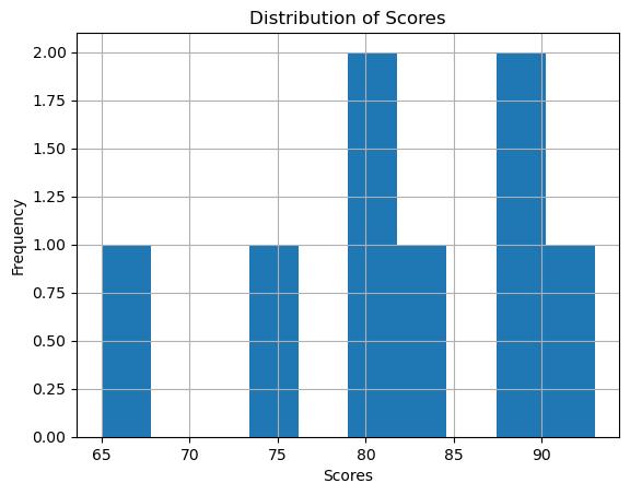
Figure1: Imagegeneratedbytheprovidedcode.
Boxplot
Boxplotsareusefulforvisualizingthedistributionofdatathroughtheirquartiles anddetectingoutliers.Here’showtocreateboxplotsformultiplecolumns:
1 #SampleDataFrame
2 data ={'math_scores':[88,76,90,84,65],
3 'eng_scores':[78,82,88,91,73]}
4 df = pd.DataFrame(data) 5 6 #Creatingaboxplot
7 df.boxplot(column =['math_scores' , 'eng_scores'])
8 plt.title('ScoreDistribution')
9 plt.ylabel('Scores')
10 plt.show()
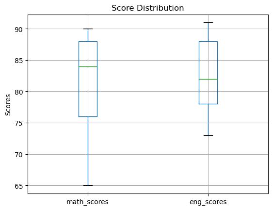
Figure2: Imagegeneratedbytheprovidedcode.
Scatterplotsareidealforexaminingtherelationshipbetweentwonumericvariables.Here’showtocreateascatterplot:
1 #SampleDataFrame
2 data ={'hours_studied':[10,15,8,12,6], 3 'test_score':[95,80,88,90,70]}
4 df = pd.DataFrame(data) 5 6 #Creatingascatterplot
7 df.plot.scatter(x = 'hours_studied' , y = 'test_score' , c = 'DarkBlue')
8 plt.title('TestScorevsHoursStudied')
9 plt.xlabel('HoursStudied')
10 plt.ylabel('TestScore')
11 plt.show()
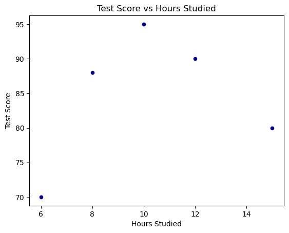
Figure3: Imagegeneratedbytheprovidedcode.
Lineplotsareusedtovisualizedatapointsconnectedbystraightlinesegments. Thisisparticularlyusefulintimeseriesanalysis: 1 #SampleDataFrame
2 data ={'year':[2010,2011,2012,2013,2014], 3 'sales':[200,220,250,270,300]}
4 df = pd.DataFrame(data) 5 6 #Creatingalineplot
7 df.plot.line(x = 'year' , y = 'sales' , color = 'red')
8 plt.title('YearlySales')
9 plt.xlabel('Year')
10 plt.ylabel('Sales')
11 plt.show()
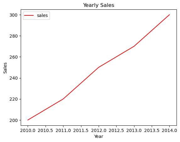
Figure4: Imagegeneratedbytheprovidedcode.
BarChart
Barchartsareusedtocomparedi erentgroups.Here’sanexampleofabarchart visualizingthecountofvaluesinacolumn:
1 #SampleDataFrame
2 data ={'product':['Apples' , 'Oranges' , 'Bananas' , ' Apples' , 'Oranges' , 'Apples']}
3 df = pd.DataFrame(data) 4
5 #Creatingabarchart
6 df['product'].value_counts().plot.bar(color = 'green')
7 plt.title('ProductFrequency')
8 plt.xlabel('Product')
9 plt.ylabel('Frequency')
10 plt.show()
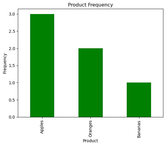
Figure5: Imagegeneratedbytheprovidedcode.
Eachofthesevisualizationtechniquesprovidesinsightsintodi erentaspectsof yourdata,makingiteasiertoperformcomprehensivedataanalysisandinterpretation.
Statisticalanalysisisakeycomponentofdataanalysis,helpingtounderstand trends,relationships,anddistributionsindata.Pandaso ersarangeoffunctions forperformingstatisticalanalyses,whichcanbeincrediblyinsightfulwhenexploringyourdata.Thischapterwillcoverthebasics,includingcorrelation,covariance, andvariouswaysofsummarizingdatadistributions.
Acorrelationmatrixdisplaysthecorrelationcoe icientsbetweenvariables.Each cellinthetableshowsthecorrelationbetweentwovariables.Here’showtogenerateacorrelationmatrix:
Thecovariancematrixissimilartoacorrelationmatrixbutshowsthecovariance betweenvariables.Here’showtogenerateacovariancematrix: 1 #Creatingacovariancematrix 2 cov_matrix = df.cov() 3 print(cov_matrix)
Thisfunctionisusedtocountthenumberofuniqueentriesinacolumn,whichcan beparticularlyusefulforcategoricaldata:
Tofinduniquevaluesinacolumn,usethe unique function.Thiscanhelpidentify thediversityofentriesinacolumn:
1 #Gettinguniquevaluesfromthecolumn
2 unique_values = df['department'].unique()
(unique_values)
Ifyouneedtoknowhowmanyuniquevaluesareinacolumn,use nunique:
1 #Countinguniquevalues
2 num_unique_values = df['department'].nunique()
3 print(num_unique_values)
Thesetoolsprovideafundamentalinsightintothestatisticalcharacteristicsofyour data,essentialforbothpreliminarydataexplorationandadvancedanalyses.
E ectivedatamanipulationinPandaso eninvolvespreciseindexingandselection toisolatespecificdatasegments.Thischapterdemonstratesseveralmethodsto selectcolumnsandrowsinaDataFrame,enablingrefineddataanalysis.
Toselectmultiplecolumns,usealistofcolumnnames.Theresultisanew DataFrame:
Youcanselectrowsbasedontheirpositionusing iloc,whichisprimarilyinteger positionbased:
Toselectrowsbylabelindex,use loc,whichuseslabelsintheindex:
1 #Selectingrowsbylabel
2 selected_rows_by_label = df.loc[0:1] 3 print(selected_rows_by_label)
1 nameage 2 0 Alice 25 3 1 Bob 30
Forconditionalselection,useaconditionwithinbracketstofilterdatabasedon columnvalues:
1 #Conditionalselection
2 condition_selected = df[df['age']>30] 3 print(condition_selected) Result:
nameage 2 2 Charlie 35
ThisselectionandindexingfunctionalityinPandasallowsforflexibleande icient datamanipulations,formingthebasisofmanydataoperationsyou’llperform.
Datao enneedstobeformattedorconvertedtodi erenttypestomeettherequirementsofvariousanalysistasks.Pandasprovidesversatilecapabilitiesfordata formattingandtypeconversion,allowingfore ectivemanipulationandpreparationofdata.Thischaptercoverssomeessentialoperationsfordataformattingand conversion.
ChangingthedatatypeofacolumninaDataFrameiso ennecessaryduringdata cleaningandpreparation.Use astype toconvertthedatatypeofacolumn:
={'age':['25' , '30' , '35']}
df['age']= df['age'].astype(int)
(df['age'].dtypes)
'age' columntointeger
PandascanperformvectorizedstringoperationsonSeriesusing .str.Thisis usefulforcleaningandtransformingtextdata:
#SampleDataFrame 2 data ={'name':['Alice' , 'Bob' , 'Charlie']} 3 df = pd.DataFrame(data)
5 #Convertingallnamestolowercase 6 df['name']= df['name'].str.lower() 7 print(df)
Convertingstringsorotherdatetimeformatsintoastandardized datetime64 typeisessentialfortimeseriesanalysis.Use pd.to_datetime toconverta column: 1 #SampleDataFrame 2 data ={'date':['2023-01-01' , '2023-01-02' , '2023-01-03' ]} 3 df = pd.DataFrame(data)
#Converting 'date' columntodatetime 6 df['date']= pd.to_datetime(df['date']) 7 print(df['date'].dtypes) Result: Page42IbonMartínez-Arranz
SettingaspecificcolumnastheindexofaDataFramecanfacilitatefastersearches, betteralignment,andeasieraccesstorows:
Theseformattingandconversiontechniquesarecrucialforpreparingyourdataset fordetailedanalysisandensuringcompatibilityacrossdi erentanalysisandvisualizationtools.
Advanceddatatransformationinvolvessophisticatedtechniquesthathelpinreshaping,restructuring,andsummarizingcomplexdatasets.Thischapterdelves intosomeofthemoreadvancedfunctionsavailableinPandasthatenabledetailed manipulationandtransformationofdata.
Lambdafunctionsprovideaquickande icientwayofapplyinganoperationacross aDataFrame.Here’showyoucanuse apply withalambdafunctiontoincrement everyelementintheDataFrame:
The melt functionisusedtotransformdatafromwideformattolongformat, whichcanbemoresuitableforanalysis:
(unstacked)
Crosstabulationsareusedtocomputeasimplecross-tabulationoftwo(ormore) factors.Thiscanbeveryusefulinstatisticsandprobabilityanalysis: 1 #Cross-tabulationexample 2 data ={'Gender':['Female' , 'Male' , 'Female' , 'Male'], 3 'Handedness':['Right' , 'Left' , 'Right' , 'Right' ]} 4 df = pd.DataFrame(data)
#Creatingacrosstabulation 7 crosstab = pd.crosstab(df['Gender'], df['Handedness'])
Theseadvancedtransformationsenablesophisticatedhandlingofdatastructures, enhancingtheabilitytoanalyzecomplexdatasetse ectively.
Timeseriesdataanalysisisacrucialaspectofmanyfieldssuchasfinance,economics,andmeteorology.Pandasprovidesrobusttoolsforworkingwithtime seriesdata,allowingfordetailedanalysisoftime-stampedinformation.Thischapterwillexplorehowtomanipulatetimeseriesdatae ectivelyusingPandas.
Settingadatetimeindexisfoundationalintimeseriesanalysisasitfacilitateseasier slicing,aggregation,andresamplingofdata:
3 #SampleDataFramewithdateinformation 4 data ={'date':['2023-01-01' , '2023-01-02' , '2023-01-03' , '2023-01-04'], 5 'value':[100,110,120,130]} 6 df = pd.DataFrame(data)
#Converting 'date' columntodatetimeandsettingitas index
9 df['date']= pd.to_datetime(df['date']) 10 df = df.set_index('date')
print(df)
Resamplingisapowerfulmethodfortimeseriesdataaggregationordownsampling, whichchangesthefrequencyofyourdata:
1 #Resamplingthedatamonthlyandcalculatingthemean 2 monthly_mean = df.resample('M').mean()
Rollingwindowoperationsareusefulforsmoothingorcalculatingmovingaverages, whichcanhelpinidentifyingtrendsintimeseriesdata:
1 #Addingmoredatapointsforabetterrollingexample 2 additional_data ={'date': pd.date_range('2023-01-05' , periods =5, freq = 'D'), 3 'value':[140,150,160,170,180]}
4 additional_df = pd.DataFrame(additional_data)
5 df = pd.concat([df, additional_df.set_index('date')])
7 #Calculatingrollingmeanwithawindowof5days
Thesetechniquesareessentialforanalyzingtimeseriesdatae iciently,providing thetoolsneededtohandletrends,seasonality,andothertemporalstructuresin data.
Oncedataanalysisiscomplete,itiso ennecessarytoexportdataintovarious formatsforreporting,furtheranalysis,orsharing.Pandasprovidesversatiletools toexportdatatodi erentfileformats,includingCSV,Excel,andSQLdatabases. ThischapterwillcoverhowtoexportDataFramestothesecommonformats.
ExportingaDataFrametoaCSVfileisstraightforwardandoneofthemostcommon methodsfordatasharing:
ThisfunctionwillcreateaCSVfilenamed filename.csv inthecurrentdirectory withouttheindexcolumn.
ExportingdatatoanExcelfilecanbedoneusingthe to_excel method,which allowsforthestorageofdataalongwithformattingthatcanbeusefulforreports:
1 #WritingtheDataFrametoanExcelfile
2 df.to_excel('filename.xlsx' , index = False) #index= Falsetoavoidwritingrowindices
ThiswillcreateanExcelfile filename.xlsx inthecurrentdirectory.
PandascanalsoexportaDataFramedirectlytoaSQLdatabase,whichisuseful forintegratinganalysisresultsintoapplicationsorstoringdatainacentralized database:
import sqlalchemy 2 3 #CreatingaSQLconnectionengine 4 engine = sqlalchemy.create_engine('sqlite:///example.db') #ExampleusingSQLite 5 6 #WritingtheDataFrametoaSQLdatabase 7 df.to_sql('table_name' , 8 con = engine, 9 index = False, 10 if_exists = 'replace')
The to_sql functionwillcreateanewtablenamed table_name inthespecified SQLdatabaseandwritetheDataFrametothistable.The if_exists='replace ' parameterwillreplacethetableifitalreadyexists;use if_exists='append' toadddatatoanexistingtableinstead.
TheseexportfunctionalitiesenhancetheversatilityofPandas,allowingforseamPage54IbonMartínez-Arranz
lesstransitionsbetweendi erentstagesofdataprocessingandsharing.
PerformingadvancedqueriesonaDataFrameallowsforprecisedatafilteringand extraction,whichisessentialfordetailedanalysis.Thischapterexplorestheuse ofthe query functionandthe isin methodforsophisticateddataqueryingin Pandas.
The
functionallowsyoutofilterrowsbasedonaqueryexpression.It’sa powerfulwaytoselectdatadynamically:
4 4 Eve 45
Thisqueryreturnsallrowswherethe age isgreaterthan30.
The isin methodisusefulforfilteringdatarowswherethecolumnvalueisina predefinedlistofvalues.It’sespeciallyusefulforcategoricaldata:
1 #SampleDataFrame
2 data ={'name':['Alice' , 'Bob' , 'Charlie' , 'David' , 'Eve '],
3 'department':['HR' , 'Finance' , 'IT' , 'HR' , 'IT' ]}
4 df = pd.DataFrame(data)
5
6 #Filteringusingisin
7 filtered_df = df[df['department'].isin(['HR' , 'IT'])] 8 print(filtered_df) Result: 1 namedepartment 2 0 AliceHR 3 2 CharlieIT 4 3 DavidHR 5 4 EveIT
Thisexamplefiltersrowswherethe department columncontainseither‘HR’or ‘IT’.
Theseadvancedqueryingtechniquesenhancetheabilitytoperformtargeteddata analysis,allowingfortheextractionofspecificsegmentsofdatabasedoncomplex criteria.
Handlinghigh-dimensionaldatao enrequirestheuseofmulti-levelindexing, orMultiIndex,whichallowsyoutostoreandmanipulatedatawithanarbitrary numberofdimensionsinlower-dimensionaldatastructureslikeDataFrames.This chaptercoverscreatingaMultiIndexandperformingslicingoperationsonsuch structures.
MultiIndexingenhancesdataaggregationandgroupingcapabilities.Itallowsfor morecomplexdatamanipulationsandmoresophisticatedanalysis:
SlicingaDataFramewithaMultiIndexinvolvesspecifyingtherangesforeachlevel oftheindex,whichcanbedoneusingthe slice functionorbyspecifyingindex valuesdirectly:
ThisexampledemonstratesslicingtheDataFrametoincludedatafromstates‘CA’
TheseMultiIndexoperationsareessentialforworkingwithcomplexdatastructures e ectively,enablingmorenuanceddataretrievalandmanipulation.
Mergingdataisafundamentalaspectofmanydataanalysistasks,especiallywhen combininginformationfrommultiplesources.Pandasprovidespowerfulfunctions tomergeDataFramesinamannersimilartoSQLjoins.Thischapterwillcoverfour primarytypesofmerges:outer,inner,le ,andrightjoins.
Anouterjoinreturnsallrecordswhenthereisamatchineitherthele orright DataFrame.Ifthereisnomatch,themissingsidewillcontain NaN. 1 import pandasaspd
4 data1 ={'column':['A' , 'B' , 'C'], 5 'values1':[1,2,3]}
6 df1 = pd.DataFrame(data1)
7 data2 ={'column':['B' , 'C' , 'D'],
8 'values2':[4,5,6]}
9 df2 = pd.DataFrame(data2)
11 #Performinganouterjoin
12 outer_joined = pd.merge(df1, df2, on = 'column' , how = ' outer')
13 print(outer_joined) Result:
1
AninnerjoinreturnsrecordsthathavematchingvaluesinbothDataFrames.
1 #Performinganinnerjoin 2 inner_joined =
3 print(inner_joined)
Ale joinreturnsallrecordsfromthele DataFrame,andthematchedrecordsfrom therightDataFrame.Theresultis NaN intherightsidewherethereisnomatch.
1 #Performingaleftjoin
Result:
(left_joined)
1
ArightjoinreturnsallrecordsfromtherightDataFrame,andthematchedrecords fromthele DataFrame.Theresultis NaN inthele sidewherethereisnomatch.
1 #Performingarightjoin 2 right_joined = pd.merge(df1, df2, on = 'column' , how = ' right')
3 print(right_joined)
Thesedatamergingtechniquesarecrucialforcombiningdatafromdi erent sources,allowingformorecomprehensiveanalysesbycreatingaunifieddataset frommultipledisparatesources.
Duplicatedatacanskewanalysisandleadtoincorrectconclusions,makingitessentialtoidentifyandhandleduplicatese ectively.Pandasprovidesstraightforward toolstofindandremoveduplicatesinyourdatasets.Thischapterwillguideyou throughtheseprocesses.
The duplicated() functionreturnsabooleanseriesindicatingwhethereach rowisaduplicateofarowthatappearedearlierintheDataFrame.Here’showto useit:
Inthisoutput, True indicatesthattherowisaduplicateofanearlierrowinthe DataFrame.
ToremovetheduplicaterowsfromtheDataFrame,usethe drop_duplicates () function.Bydefault,thisfunctionkeepsthefirstoccurrenceandremoves subsequentduplicates.
1
Thismethodhasremovedrows3and4,whichwereduplicatesofearlierrows.You canalsocustomizethisbehaviorwiththe keep parameter,whichcanbesetto 'last' tokeepthelastoccurrenceinsteadofthefirst,or False toremoveall duplicatesentirely.
Thesetechniquesareessentialforensuringdataquality,enablingaccurateand reliabledataanalysisbymaintainingonlyuniquedataentriesinyourDataFrame.
The apply functioninPandasishighlyversatile,allowingyoutoexecutecustom functionsacrossanentireDataFrameoralongaspecifiedaxis.Thisflexibilitymakes itindispensableforperformingcomplexoperationsthatarenotdirectlysupported bybuilt-inmethods.Thischapterwilldemonstratehowtouse apply forcustom operations.
Using apply withalambdafunctionallowsyoutodefineinlinefunctionstoapply toeachroworcolumnofaDataFrame.Hereishowyoucanuseacustomfunction toprocessdatarow-wise:
Inthisexample,the custom_func isappliedtoeachrowoftheDataFrameusing apply.Thefunctioncalculatesanewvaluebasedoncolumns‘col1’and‘col2’for eachrow,andtheresultsarestoredinanewcolumn‘result’.
Thismethodofapplyingcustomfunctionsispowerfulfordatamanipulationand transformation,allowingforoperationsthatgobeyondsimplearithmeticoraggregation.It’sparticularlyusefulwhenyouneedtoperformoperationsthatare specifictoyourdataandnotprovidedbyPandas’built-inmethods.
Visualizingdataisakeystepindataanalysis,providinginsightsthatarenotapparentfromrawdataalone.PandasintegratessmoothlywithMatplotlib,apopular plottinglibraryinPython,too erversatileoptionsfordatavisualization.This chapterwillshowhowtocreatecustomplotsusingPandasandMatplotlib.
Pandas’plottingcapabilitiesarebuiltonMatplotlib,allowingforstraightforward generationofvarioustypesofplotsdirectlyfromDataFrameandSeriesobjects.
Here’showtocreateasimplelineplotdisplayingtrendsoveraseriesofvalues:
import matplotlib.pyplotasplt
#Sampledata
data ={'Year':[2010,2011,2012,2013,2014], 6 'Sales':[100,150,200,250,300]}
df = pd.DataFrame(data)
9 #Plotting
10 df.plot(x = 'Year' , y = 'Sales' , kind = 'line')
11 plt.title('YearlySales')
12 plt.ylabel('Sales')
13 plt.show()
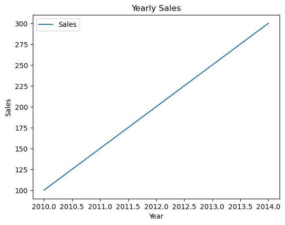
Figure1: Imagegeneratedbytheprovidedcode.
Histogram
Histogramsaregreatforvisualizingthedistributionofnumericaldata:
1 #Sampledata
2 data ={'Grades':[88,92,80,89,90,78,84,76,95, 92]} 3 df = pd.DataFrame(data) 4 5 #Plottingahistogram
6 df['Grades']\ 7 .plot(kind = 'hist' , 8 bins =5, 9 alpha =0.7)
10 plt.title('DistributionofGrades')
11 plt.xlabel('Grades')
12 plt.show()
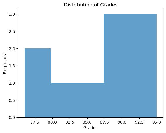
Figure2: Imagegeneratedbytheprovidedcode.
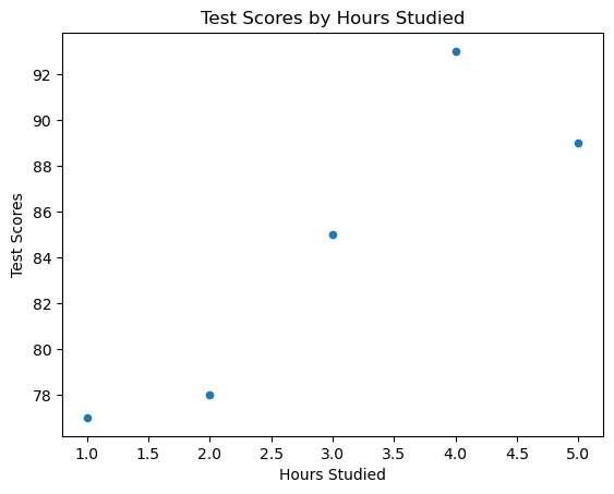
Scatterplotsareusedtoobserverelationshipsbetweenvariables:
1 #Sampledata
2 data ={'Hours':[1,2,3,4,5], 3 'Scores':[77,78,85,93,89]} 4 df = pd.DataFrame(data) 5 6 #Creatingascatterplot
7 df.plot(kind = 'scatter' , x = 'Hours' , y = 'Scores')
8 plt.title('TestScoresbyHoursStudied')
9 plt.xlabel('HoursStudied')
10 plt.ylabel('TestScores')
11 plt.show()
8 x = 'Bars' , 9 y = 'Values' , 10 color = 'blue' , 11 legend = None)
12 plt.title('BarChartExample')
13 plt.ylabel('Values')
14 plt.show()
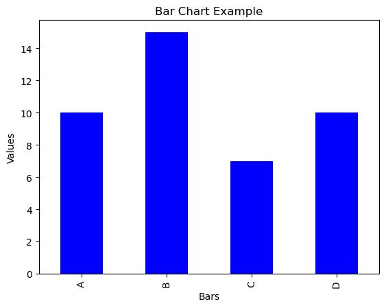
Figure4: Imagegeneratedbytheprovidedcode.
TheseexamplesillustratehowtointegratePandaswithMatplotlibtocreateinformativeandvisuallyappealingplots.Thisintegrationisvitalforanalyzingtrends, distributions,relationships,andpatternsindatae ectively.
Groupingandaggregatingdataarefundamentaloperationsindataanalysis,especiallywhendealingwithlargeorcomplexdatasets.Pandaso ersadvanced capabilitiesthatallowforsophisticatedgroupingandaggregationstrategies.This chapterexploressomeoftheseadvancedtechniques,includinggroupingbymultiplecolumns,usingmultipleaggregationfunctions,andapplyingtransformation functions.
Groupingbymultiplecolumnsallowsyoutoperformmoredetailedanalysis.Here’s howtocomputethemeanofgroupsdefinedbymultiplecolumns:
Thisexampledemonstrateshowtonormalizethe‘Revenue’withineach‘Department’,showingdeviationsfromthedepartmentmeanintermsofstandarddeviations.
Theseadvancedgroupingandaggregationtechniquesprovidepowerfultoolsfor breakingdowncomplexdataintomeaningfulsummaries,enablingmorenuanced analysisandinsights.
Textdatao enrequiresspecificprocessingtechniquestoextractmeaningfulinformationortoreformatitforfurtheranalysis.Pandasprovidesarobustsetofstring operationsthatcanbeappliede icientlytoSeriesandDataFrames.Thischapter exploressomeessentialoperationsforhandlingtextdata,includingsearchingfor substrings,splittingstrings,andusingregularexpressions.
The contains methodallowsyoutofilterrowsbasedonwhetheracolumn’stext containsaspecifiedsubstring.Thisisusefulforsubsettingdatabasedontextual content:
Splittingstringsintoseparatecomponentscanbeessentialfordatacleaningand preparation.The split methodsplitseachstringintheSeries/Indexbythegiven delimiterandoptionallyexpandstoseparatecolumns:
1 #SplittingtheDescriptioncolumnintowords
2 split_description = df['Description'].str.split('' , expand = True)
3 print(split_description)
Thissplitsthe‘Description’columnintoseparatecolumnsforeachword.
Regularexpressionsareapowerfultoolforextractingpatternsfromtext.The extract methodappliesaregularexpressionpatternandextractsgroupsfrom thefirstmatch:
1 #Extractingthefirstwordwhereitstartswitha
2 #capitalletterfollowedbylowercaseletters
3 extracted_words = df['Description'].str.extract(r'([A-Z][ a-z]+)')
Thisregularexpressionextractsthefirstwordfromeachdescription,whichstarts withacapitalletterandisfollowedbylowercaseletters.
Thesetext-specificoperationsinPandassimplifytheprocessofworkingwithtextual data,allowingfore icientandpowerfulstringmanipulationandanalysis.
Intoday’sdata-drivenworld,JSON(JavaScriptObjectNotation)andXML(eXtensibleMarkupLanguage)aretwoofthemostcommonformatsusedforstoringand transferringdataontheweb.Pandasprovidesbuilt-infunctionstoeasilyread theseformatsintoDataFrames,facilitatingtheanalysisofstructureddata.This chapterexplainshowtoreadJSONandXMLfilesusingPandas.
JSONisalightweightformatthatiseasyforhumanstoreadandwrite,andeasy formachinestoparseandgenerate.PandascandirectlyreadJSONdataintoa DataFrame:
#ReadingJSONdata 4 df = pd.read_json('filename.json') 5 print(df)
ThismethodwillconvertaJSONfileintoaDataFrame.ThekeysoftheJSONobject willcorrespondtocolumnnames,andthevalueswillformthedataentriesforthe rows.
XMLisusedforrepresentingdocumentswithastructuredmarkup.Itismore verbosethanJSONbutallowsforamorestructuredhierarchy.Pandascanread XMLdataintoaDataFrame,similartohowitreadsJSON:
1 #ReadingXMLdata
2 df = pd.read_xml('filename.xml')
3 print(df)
ThiswillparseanXMLfileandcreateaDataFrame.ThetagsoftheXMLfilewill typicallydefinethecolumns,andtheirrespectivecontentwillbethedataforthe rows.
Thesefunctionalitiesallowforseamlessintegrationofdatafromwebsourcesand othersystemsthatutilizeJSONorXMLfordatainterchange.ByleveragingPandas’ abilitytoworkwiththeseformats,analystscanfocusmoreonanalyzingthedata ratherthanspendingtimeondatapreparation.
Handlingfileswithvariousconfigurationsandformatsisacommonnecessityin dataanalysis.Pandasprovidesextensivecapabilitiesforreadingfromandwriting todi erentfiletypeswithvaryingdelimitersandformats.Thischapterwillexplore readingCSVfileswithspecificdelimitersandwritingDataFramestoJSONfiles.
CSVfilescancomewithdi erentdelimiterslikecommas(,),semicolons(;),or tabs(\t).Pandasallowsyoutospecifythedelimiterwhenreadingthesefiles, whichiscrucialforcorrectlyparsingthedata.
IftheCSVfileusestabsasdelimiters,here’showyoumightseethefileandread it:
WritingdatatoJSONformatcanbeusefulforwebapplicationsandAPIs.Here’s howtowriteaDataFrametoaJSONfile:
1 #DataFrametowritetoJSON
2 df.to_json('filename.json')
Assuming df containsthepreviousdata,theJSONfile filename.json would looklikethis:
1 {"Name":{"0":"Alice","1":"Bob","2":"Charlie"},"Age":{"0" :30,"1":25,"2":35},"City":{"0":"NewYork","1":"Los Angeles","2":"Chicago"}}
Thisformatisknownas‘column-oriented’JSON.PandasalsosupportsotherJSON orientationswhichcanbespecifiedusingthe orient parameter.
Theseadvancedfilehandlingtechniquesensurethatyoucanworkwithawide rangeoffileformatsandconfigurations,facilitatingdatasharingandintegration acrossdi erentsystemsandapplications.
Missingdatacansignificantlyimpacttheresultsofyourdataanalysisifnotproperly handled.Pandasprovidesseveralmethodstodealwithmissingvalues,allowing youtoeitherfillthesegapsormakeinterpolationsbasedontheexistingdata. Thischapterexploresmethodslikeinterpolation,forwardfilling,andbackward filling.
Interpolationisamethodofestimatingmissingvaluesbyusingotheravailable datapoints.Itisparticularlyusefulintimeseriesdatawherethiscanestimatethe trendsaccurately:
Here, interpolate() linearlyestimatesthemissingvaluesbetweentheexisting numbers.
Forwardfill(ffill)propagatesthelastobservednon-nullvalueforwarduntil anothernon-nullvalueisencountered:
1 #SampleDataFramewithmissingvalues
2 data ={'value':[1, np.nan, np.nan,4,5]}
3 df = pd.DataFrame(data)
4
5 #Applyingforwardfill
6 df['value'].ffill(inplace = True) 7 print(df) Result:
value
Backwardfill(bfill)propagatesthenextobservednon-nullvaluebackwards untilanothernon-nullvalueismet:
Thesemethodsprovideyouwithflexibleoptionsforhandlingmissingdatabasedon thenatureofyourdatasetandthespecificrequirementsofyouranalysis.Correctly addressingmissingdataiscrucialformaintainingtheaccuracyandreliabilityof youranalyticalresults.
Datareshapingisacrucialaspectofdatapreparationthatinvolvestransformingdatabetweenwideformat(withmorecolumns)andlongformat(withmore rows),dependingontheneedsofyouranalysis.Thischapterdemonstrateshowto reshapedatafromwidetolongformatsandviceversausingPandas.
The wide_to_long functioninPandasisapowerfultoolfortransformingdata fromwideformattolongformat,whichiso enmoreamenabletoanalysisin Pandas:
ThisoutputrepresentsaDataFrameinlongformatwhereeachrowcorrespondsto asingleyearforeachvariable(AandB)andeachid.
Convertingdatafromlongtowideformatinvolvescreatingapivottable,which cansimplifycertaintypesofdataanalysisbydisplayingdatawithonevariableper columnandcombinationsofothervariablesperrow:
1 #Assuminglong_dfistheDataFrameinlongformatfrom thepreviousexample 2 #Wewilluseaslightmodificationforclarity 3 long_data ={ 4 'id':[1,1,2,2], 5 'year':[2020,2021,2020,2021], 6 'A':[100,150,200,250], 7 'B':[300,350,400,450]
} 9 long_df = pd.DataFrame(long_data)
#Transformingfromlongtowideformat 12 wide_df = long_df.pivot(index = 'id' , columns = 'year') 13 print(wide_df)
ThisresultdemonstratesaDataFrameinwideformatwhereeach id hasassociated valuesofAandBforeachyearspreadacrossmultiplecolumns.
Reshapingdatae ectivelyallowsforeasieranalysis,particularlywhendealingwith paneldataortimeseriesthatrequireoperationsacrossdi erentdimensions.
Categoricaldataiscommoninmanydatasetsinvolvingcategoriesorlabels,such assurveyresponses,producttypes,oruserroles.E icienthandlingofsuchdata canleadtosignificantperformanceimprovementsandeaseofuseindatamanipulationandanalysis.Pandasprovidesrobustsupportforcategoricaldata,including convertingdatatypestocategoricalandspecifyingtheorderofcategories.
Convertingacolumntoacategoricaltypecanoptimizememoryusageandimprove performance,especiallyforlargedatasets.Here’showtoconvertacolumnto
7 Name: product, dtype: category
8 Categories (3, object):['apple' , 'banana' , 'orange']
Thisshowsthatthe‘product’columnisnowoftype category withthreecategories.
Sometimes,thenaturalorderofcategoriesmatters(e.g.,inordinaldatasuchas ‘low’,‘medium’,‘high’).Pandasallowsyoutosetandordercategories:
1 #SampleDataFramewithunorderedcategoricaldata
2 data ={'size':['medium' , 'small' , 'large' , 'small' , ' large' , 'medium']}
3 df = pd.DataFrame(data)
4 df['size']= df['size'].astype('category') 5 6 #Settingandorderingcategories
7 df['size']= df['size'].cat.set_categories(['small' , ' medium' , 'large'], ordered = True,)
8 print(df['size'])
7 Name: size, dtype: category
8 Categories (3, object):['small' < 'medium' < 'large']
Thisconversionandorderingprocessensuresthatthe‘size’columnisnotonly categoricalbutalsocorrectlyorderedfrom‘small’to‘large’.
ThesecategoricaldataoperationsinPandasfacilitatethee ectivehandlingofnominalandordinaldata,enhancingbothperformanceandthecapacityformeaningful dataanalysis.
AdvancedindexingtechniquesinPandasenhancedatamanipulationcapabilities, allowingformoresophisticateddataretrievalandmodificationoperations.This chapterwillfocusonresettingindexes,settingmultipleindexes,andslicingthrough MultiIndexes,whicharecrucialforhandlingcomplexdatasetse ectively.
ResettingtheindexofaDataFramecanbeusefulwhentheindexneedstobetreated asaregularcolumn,orwhenyouwanttoreverttheindexbacktothedefaultinteger index:
2 039500000 3 119500000 4 221400000
Using drop=True removestheoriginalindexandjustkeepsthedatacolumns.
Settingmultiplecolumnsasanindexcanprovidepowerfulwaystoorganizeand selectdata,especiallyusefulinpaneldataorhierarchicaldatasets:
1 #Re-usingpreviousDataFramewithoutresetting
2 df = pd.DataFrame(data)
3
4 #Settingmultiplecolumnsasanindex
5 df.set_index(['state' , 'population'], inplace = True)
6 print(df) Result:
1 EmptyDataFrame
2 Columns:[]
3 Index:[(CA,39500000),(NY,19500000),(FL,21400000)]
TheDataFramenowusesacompositeindexmadeupof‘state’and‘population’.
SlicingdatawithaMultiIndexcanbecomplexbutpowerful.The xs method(crosssection)isoneofthemostconvenientwaystoslicemulti-levelindexes:
1 #AssumingtheDataFramewithaMultiIndexfromthe previousexample
2 #Addingsomevaluestodemonstrateslicing
#Slicingwithxs 6 slice_df = df.xs(key = 'CA' , level = 'state')
Thisoperationretrievesallrowsassociatedwith‘CA’fromthe‘state’levelofthe index,showingonlythedataforthepopulationofCalifornia.
Advancedindexingtechniquesprovidenuancedcontroloverdataaccesspatterns inPandas,enhancingdataanalysisandmanipulationcapabilitiesinawiderange ofapplications.
E icientcomputationiskeyinhandlinglargedatasetsorperformingcomplex operationsrapidly.Pandasincludesfeaturesthatleverageoptimizedcodepaths tospeedupoperationsandreducememoryusage.Thischapterdiscussesusing eval() forarithmeticoperationsandthe query() methodforfiltering,which arebothdesignedtoenhanceperformance.
The eval() functioninPandasallowsfortheevaluationofstringexpressions usingDataFramecolumns,whichcanbesignificantlyfaster,especiallyforlarge DataFrames,asitavoidsintermediatedatacopies:
data ={'col1':[1,2,3],
'col2':[4,5,6]}
#Usingeval()toperformefficientoperations 9 df['col3']= df.eval('col1+col2')
2 0145
3 1257 4 2369
Thisexampledemonstrateshowtoaddtwocolumnsusing eval(),whichcanbe fasterthantraditionalmethodsforlargedatasetsduetooptimizedcomputation.
The query() methodallowsyoutofilterDataFramerowsusinganintuitive querystring,whichcanbemorereadableandperformantcomparedtotraditional Booleanindexing:
1 #SampleDataFrame
2 data ={'col1':[10,20,30],
3 'col2':[20,15,25]}
4 df = pd.DataFrame(data)
5
6 #Usingquery()tofilterdata
7 filtered_df = df.query('col1<col2')
8 print(filtered_df)
Result:
1 col1col2 2 01020
Inthisexample, query() filterstheDataFrameforrowswhere‘col1’islessthan ‘col2’.Thismethodcanbeespeciallye icientwhenworkingwithlargeDataFrames, asitutilizesnumexprforfastevaluationofarrayexpressions.
ThesemethodsenhancePandas’performance,makingitapowerfultoolfordata analysis,particularlywhenworkingwithlargeorcomplexdatasets.E icientcomputationsensurethatresourcesareoptimallyused,speedingupdataprocessing andanalysis.
Combiningdatasetsisacommonrequirementindataanalysis.Beyondbasic merges,Pandaso ersadvancedtechniquessimilartoSQLoperationsandallows concatenationalongdi erentaxes.ThischapterexploresSQL-likejoinsandvarious concatenationmethodstoe ectivelycombinemultipledatasets.
SQL-likejoinsinPandasareachievedusingthe merge function.Thismethodis extremelyversatile,allowingforinner,outer,le ,andrightjoins.Here’showto performale join,whichincludesallrecordsfromthele DataFrameandthe matchedrecordsfromtherightDataFrame.Ifthereisnomatch,theresultis NaN onthesideoftherightDataFrame.
1 import pandasaspd 2
3 #SampleDataFrames
4 data1 ={'col':['A' , 'B' , 'C'], 5 'col1':[1,2,3]}
6 df1 = pd.DataFrame(data1)
7 data2 ={'col':['B' , 'C' , 'D'],
8 'col2':[4,5,6]}
9 df2 = pd.DataFrame(data2)
10
11 #Performingaleftjoin
12 left_joined_df = pd.merge(df1, df2, how = 'left' , on = ' col')
13 print(left_joined_df)
Result:
1 colcol1col2 2
Thisresultshowsthatallentriesfrom df1 areincluded,andwherethereare matching‘col’valuesin df2,the‘col2’valuesarealsoincluded.
Concatenationcanbeperformednotjustvertically(defaultaxis=0),butalsohorizontally(axis=1).Thisisusefulwhenyouwanttoaddnewcolumnstoanexisting DataFrame:
1 #Concatenatingdf1anddf2alongaxis1
2 concatenated_df = pd.concat([df1, df2], axis =1)
3 print(concatenated_df)
Result: 1 colcol1colcol2
ThisresultdemonstratesthattheDataFramesareconcatenatedside-by-side,aligningbyindex.Notethatbecausethe‘col’valuesdonotmatchbetween df1 and df2,theyappeardisjointed,illustratingtheimportanceofindexalignmentinsuch operations.
Theseadvanceddatamergingtechniquesprovidepowerfultoolsfordataintegration,allowingforcomplexmanipulationsandcombinationsofdatasets,muchlike Page108IbonMartínez-Arranz
youwouldaccomplishusingSQLinadatabaseenvironment.
Ensuringdataqualityisacriticalstepinanydataanalysisprocess.Datao en comeswithissueslikemissingvalues,incorrectformats,oroutliers,whichcan significantlyimpactanalysisresults.Pandasprovidestoolstoperformthesechecks e iciently.Thischapterfocusesonusingassertionstovalidatedataquality.
The assert statementinPythonisane ectivewaytoensurethatcertainconditionsaremetinyourdata.Itisusedtoperformsanitychecksandcanhaltthe programiftheassertionfails,whichishelpfulinidentifyingdataqualityissues earlyinthedataprocessingpipeline.
OnecommoncheckistoensurethattherearenomissingvaluesinyourDataFrame. Here’showyoucanusean assert statementtoverifythattherearenomissing valuesacrosstheentireDataFrame:
4 #SampleDataFramewithpossiblemissingvalues
5 data ={'col1':[1,2, np.nan], 'col2':[4, np.nan,6]}
6 df = pd.DataFrame(data)
7
8 #Assertiontocheckformissingvalues
9 try:
10 assertdf.notnull().all().all(), "Therearemissing valuesinthedataframe"
11 except AssertionErrorase: 12 print(e)
IftheDataFramecontainsmissingvalues,theassertionfails,andtheerrormessage “Therearemissingvaluesinthedataframe”isprinted.Ifnomissingvaluesare present,thescriptcontinueswithoutinterruption.
Thismethodofdatavalidationhelpsinenforcingthatdatameetstheexpectedqualitystandardsbeforeproceedingwithfurtheranalysis,thussafeguardingagainst analysisbasedonfaultydata.
ThiscodeloadstheTitanicdatasetdirectlyfromapubliclyaccessibleURLinto aPandasDataFrameandprintsthefirstfewentriestogetapreliminaryviewof thedataanditsstructure.The info() functionisthenusedtoprovideaconcise summaryoftheDataFrame,detailingthenon-nullcountanddatatypeforeach column.Thissummaryisinvaluableforquicklyidentifyinganymissingdataand understandingthedatatypespresentineachcolumn,settingthestageforfurther datamanipulationandanalysis.
18
14 alone
non-null bool
dtypes: bool(2), float64(2), int64(4), object(7)
Thissectiongeneratesstatisticalsummariesfornumericalcolumnsusingdescribe(), whichprovidesaquickoverviewofcentraltendencies,dispersion,andshapeof thedataset’sdistribution.Histogramsandboxplotsareplottedtovisualizethe distributionofanddetectoutliersinnumericaldata.The value_counts() methodgivesacountofuniquevaluesforcategoricalvariables,whichhelpsin understandingthedistributionofcategoricaldata.The pairplot() function fromSeabornshowspairwiserelationshipsinthedataset,coloredbythe‘Survived’ columntoseehowvariablescorrelatewithsurvival. 1 import matplotlib.pyplotasplt
print(titanic.describe())
#Distributionofkeycategoricalfeatures 8 print(titanic['survived'].value_counts())
print(titanic['pclass'].value_counts())
print(titanic['sex'].value_counts())
titanic.hist(bins=10, figsize=(10,7))
plt.show()
titanic.boxplot(column=['age' , 'fare'])
plt.show()
#Pairplottovisualizetherelationshipsbetween numericalvariables 21 sns.pairplot(titanic.dropna(), hue = 'survived')
#Distributionofkeycategoricalfeatures 8 print(titanic['survived'].value_counts())
print(titanic['pclass'].value_counts())
(titanic['sex'].value_counts())
#Distributionofkeycategoricalfeatures 8 print(titanic['survived'].value_counts())
print(titanic['pclass'].value_counts())
print(titanic['sex'].value_counts())
1 #Histogramsfornumericalcolumns
2 titanic.hist(bins=10, figsize=(10,7))
3 plt.show()
1 #Histogramsfornumericalcolumns
2 titanic.hist(bins=10, figsize=(10,7)) 3 plt.show()
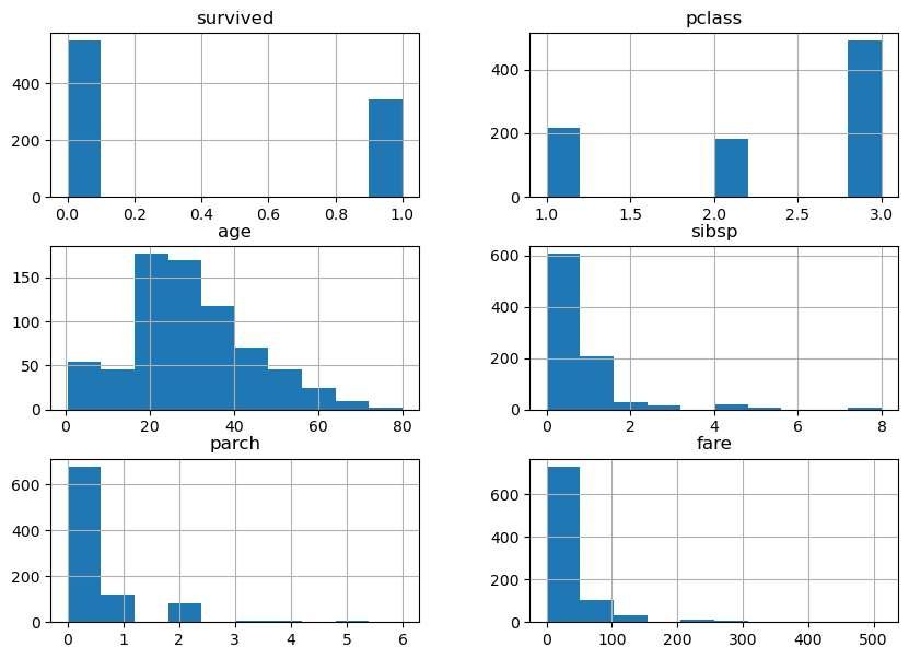
Figure1: Imagegeneratedbytheprovidedcode.
1 #Boxplotstocheckforoutliers
2 titanic.boxplot(column=['age' , 'fare'])
3 plt.show()
1 #Boxplotstocheckforoutliers
2 titanic.boxplot(column=['age' , 'fare'])
3 plt.show()
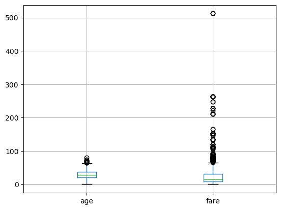
Figure2: Imagegeneratedbytheprovidedcode.
1 #Pairplottovisualizetherelationshipsbetween numericalvariables
2 sns.pairplot(titanic.dropna(), hue = 'survived') 3 plt.show()
1 #Pairplottovisualizetherelationshipsbetween numericalvariables
2 sns.pairplot(titanic.dropna(), hue = 'survived')
3 plt.show()
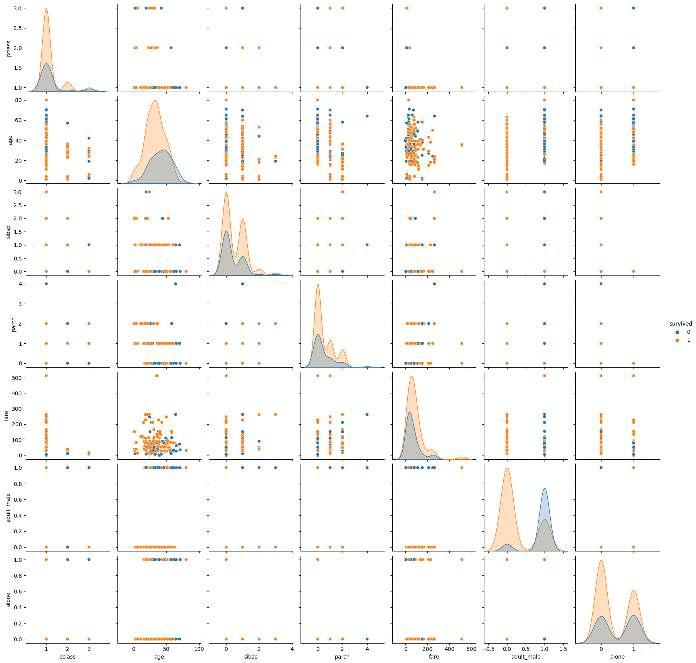
Figure3: Imagegeneratedbytheprovidedcode.
Thiscodechecksformissingvaluesandhandlesthembyfillingwithmedianvaluesfor Age andthemodefor Embarked.Itconvertscategoricaldata(Sex)intoa numericalformatsuitableformodeling.Columnsthatarenotnecessaryforthe
Thissegmentexaminessurvivalratesby class and sex.Ituses groupby() to segmentdatafollowedbymeancalculationstoanalyzesurvivalrates.Resultsare visualizedusingbarplotstoprovideaclearvisualcomparisonofsurvivalrates acrossdi erentgroups.
1 #Groupdatabysurvivalandclass
2 survival_rate = titanic.groupby('pclass')['survived']. mean()
3 print(survival_rate)
1 pclass
2 10.629630
3 20.472826
4 30.242363
5 Name: survived, dtype: float64
1 #Survivalratebysex
2 survival_sex = titanic.groupby('sex')['survived'].mean()
3 print(survival_sex)
1 sex 2 female 0.742038
3 male 0.188908
4 Name: survived, dtype: float64
1 #Visualizationofsurvivalrates
2 sns.barplot(x = 'pclass' , y = 'survived' , data=titanic)
3 plt.title('SurvivalRatesbyClass')
4 plt.show()
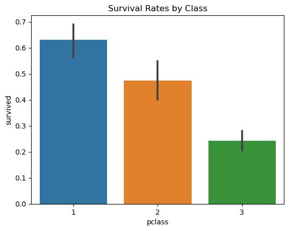
Figure4: Imagegeneratedbytheprovidedcode.
1 sns.barplot(x = 'sex' , y = 'survived' , data=titanic)
2 plt.title('SurvivalRatesbySex')
3 plt.show()
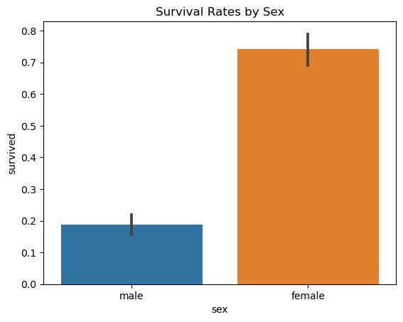
Figure5: Imagegeneratedbytheprovidedcode.
Thefinalsectionsummarizesthekeyfindingsfromtheanalysis,highlightingthe influenceoffactorslike sex and class onsurvivalrates.Italsodiscusseshowthe techniquesappliedcanbeusedwithotherdatasetstoderiveinsightsandsupport decision-makingprocesses.
1 #Summaryoffindings
2 print("KeyFindingsfromtheTitanicDataset:")
3 print("1.Highersurvivalrateswereobservedamong femalesandupper-classpassengers.")
4 print("2.Ageandfarepricesalsoappearedtoinfluence survivalchances.")
5 6 #Discussiononapplications
7 print("Theseanalysistechniquescanbeappliedtoother datasetstouncoverunderlyingpatternsandimprove decision-making.")
ProvidesadditionalresourcesforreaderstoexploremoreaboutPandasanddata analysis.Thisincludeslinkstoo icialdocumentationandtheKagglecompetition pagefortheTitanicdataset,whicho ersaplatformforpracticingandimproving dataanalysisskills.
ThiscomprehensivechapteroutlineandcodeexplanationsgivereadersathoroughunderstandingofdataanalysisworkflowsusingPandas,fromdataloadingto cleaning,analysis,anddrawingconclusions.
1 #ThissectionwouldlistURLsorreferencestofurther reading
2 print("FormoredetailedtutorialsonPandasanddata analysis,visit:")
3 print("-TheofficialPandasdocumentation:https:// pandas.pydata.org/pandas-docs/stable/")
4 print("-Kaggle'sTitanicCompetitionformore explorations:https://www.kaggle.com/c/titanic")
Thischapterprovidesathoroughwalk-throughusingtheTitanicdatasettodemonstratevariousdatahandlingandanalysistechniqueswithPandas,o eringpractical insightsandmethodsthatcanbeappliedtoawiderangeofdataanalysisscenarios.