EssentialGuide toSeaborn

Visualstorytellingmadesimple.
Masterstatisticaldatavisualizationwithseaborn.Createinformative andbeautifulplotsdirectlyfromyourdata
Visualstorytellingmadesimple.
Masterstatisticaldatavisualizationwithseaborn.Createinformative andbeautifulplotsdirectlyfromyourdata
SeabornisaPythondatavisualizationlibrarybasedonMatplotlib.Itprovides ahigh-level,user-friendlyAPIforcreatinginformativeandattractivestatistical graphics.WhileMatplotlibishighlyflexibleandpowerful,Seaborno ersasetof toolsthatmakecommonvisualizationtasksfasterandeasier,especiallywhen workingwithpandasDataFrames.
• EasyintegrationwithpandasDataFrames.
• Beautifuldefaultstyles.
• Built-infunctionsforcommonstatisticalplots.
• SimplifiedsyntaxcomparedtoMatplotlib.
• EasycustomizationandextensionwithMatplotlib.
ThisbookwillguideyouthroughthemainfunctionalitiesofSeaborn,startingfrom simpleplotsandprogressingtomoreadvancedtopicslikegrids,regressionplots, andcasestudies.
Beforestarting,youneedtoinstallSeabornanditsdependencies.Werecommend usingavirtualenvironment.
1 pipinstallseabornpandasmatplotlib
Wewillalsouse jupyter toexecuteanddisplayplotsinsidenotebooks:
1 pipinstalljupyter
Recommendedimports:
1 import seabornassns
2 import pandasaspd
3 import matplotlib.pyplotasplt
4
5 sns.set_theme() #Optionalbutrecommended
YourFirstPlot
Let’screateourfirstsimpleplottomakesureeverythingworks:
1 #Createsomedummydata
2 data = pd.DataFrame({
3 "x": range(10),
4 "y":[i **2 for i in range(10)]
5 })
6
7 sns.lineplot(data=data, x="x", y="y") 8 plt.show()
Youshouldseeasimplelineplot.
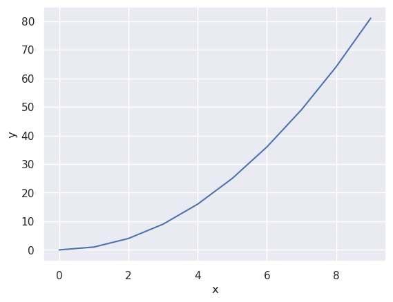
Figure1: Imagegeneratedbytheprovidedcode. DatasetsWeWillUse
Throughoutthisbook,wewillworkwithseveraldatasets: Penguinsdataset
The penguins datasetisamodernalternativetotheclassicirisdataset.ItprovidesmeasurementsofthreepenguinspeciescollectedfromislandsinPalmer Archipelago,Antarctica.
• Variables:species,island,billlength,billdepth,flipperlength,bodymass, sex,year.
Aclassicdatasetaboutrestaurantbillsandtips,includingtotalbill,tip,genderof thecustomer,smokingstatus,dayoftheweek,timeoftheday,andpartysize.
• Variables:total_bill,tip,sex,smoker,day,time,size.
Atimeseriesdatasetshowingthenumberofpassengersoveryearsandmonths. Veryusefulforlineplotsandheatmaps.
• Variables:year,month,passengers.
Inthenextchapter,wewillbeginexploring relationalplots,thebackbone ofscatterplots,lineplots,andmore.
Relationalplotsareusedtodisplayrelationshipsbetweentwoormorevariables. Thisisoneofthemostcommontasksindatavisualization,especiallywhenperformingexploratorydataanalysis(EDA).
Seabornprovidestwomainfunctionsforrelationalplots:- scatterplot() forpoint-basedvisualizations.- lineplot() fortrendortimeseriesvisualizations.
Inthischapter,wewilllearnhowtousethemstepbystep,fromthesimplestusagetoadvancedcustomizationsusingargumentssuchas hue, size,and style. Theseargumentsareespeciallyusefulwhenwewanttoencodeadditionalinformationvisually.
Thescatterplotisusedtovisualizetherelationshipbetweentwonumericvariables. Let’sstartwithasimpleexampleusingthe penguins dataset.
1 #Loaddataset
2 penguins = sns.load_dataset("penguins")
3
4 #Basicscatterplot
5 sns.scatterplot(data=penguins,
6 x="bill_length_mm",
7 y="bill_depth_mm")
8 plt.show()
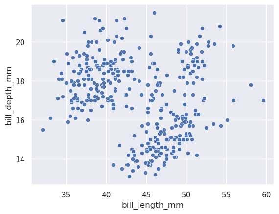
Figure1: Imagegeneratedbytheprovidedcode.
Explanation:
Eachpointrepresentsonepenguin.The x axisshowsthebilllengthandthe y axis thebilldepth.
Seabornallowsyoutoeasilymapacategoricalvariabletothecolorofthepoints usingthe hue argument.
1 sns.scatterplot(data=penguins, 2 x="bill_length_mm", 3 y="bill_depth_mm", 4 hue="species") 5 plt.show()
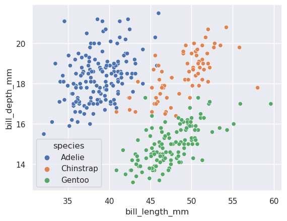
Figure2: Imagegeneratedbytheprovidedcode.
Now,eachspecieshasadi erentcolor.Thismakesiteasiertospotpatternsby species.
Youcanaddevenmoreinformationbyusingthe size and style arguments.
1 sns.scatterplot(
2 data=penguins, 3 x="bill_length_mm", 4 y="bill_depth_mm", 5 hue="species",
6 size="flipper_length_mm", 7 style="sex"
8 )
9 plt.show()
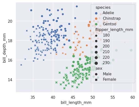
Figure3: Imagegeneratedbytheprovidedcode.
Explanation:
• Thesizeofthepointsrepresentstheflipperlength.
• Thestyle(shape)ofthepointsindicatesthesexofeachpenguin.
NoticehowSeabornautomaticallyhandleslegendswhenyouusemultipleencodings.
Lineplotsaremainlyusedtoshowtrendsoveracontinuousvariable,typicallytime orordereddata.
Let’smovetothe flights dataset,whichisperfectforthistypeofvisualization.
1 flights = sns.load_dataset("flights") 2 flights.head()
1 sns.lineplot(data=flights, x="year", y="passengers") 2 plt.show()
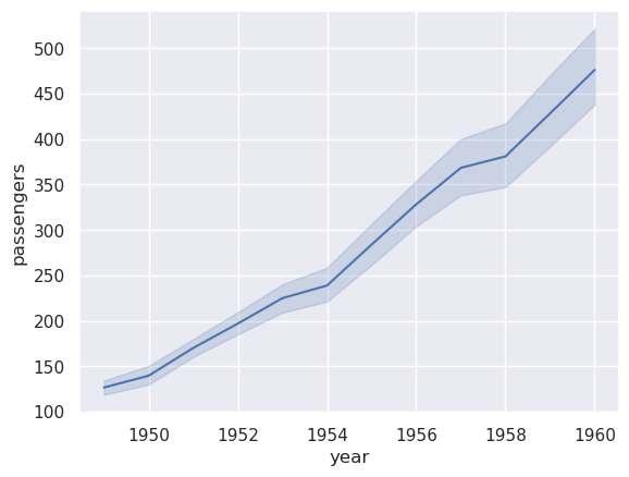
Figure4: Imagegeneratedbytheprovidedcode.
Explanation:
Thisplotshowstheaveragenumberofpassengersforeachyear,aggregatingall months.
Groupedlineplotwith hue
1 sns.lineplot(data=flights, 2 x="year", 3 y="passengers", IbonMartínez-ArranzPage15
4 hue="month") 5 plt.show()
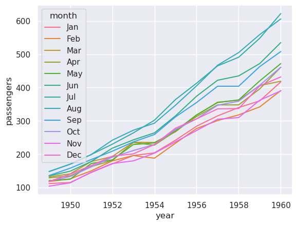
Figure5: Imagegeneratedbytheprovidedcode.
Explanation:
Nowwearesplittingthedataby month.Eachlinerepresentsamonth,makingit possibletoanalyzeseasonalityandtrendsoveryears.
Seabornmakesiteasytocombinemultipleencodings:
1 sns.lineplot( 2 data=flights, 3 x="year", 4 y="passengers", 5 hue="month", 6 style="month", 7 markers=True, 8 dashes=False 9 ) 10 plt.show()
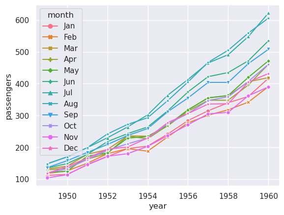
Figure6: Imagegeneratedbytheprovidedcode.
Explanation:
• Di erentmonthsnowhavebothdi erentcolorsanddi erentlinestyles (markers).
• Thisisespeciallyhelpfulwhencreatingplotsforprint,wherecoloralone mightnotbesu icient.
ArgumentDescription
hue
Mapsavariabletocolor size
Mapsavariabletomarkersize style
Mapsavariabletomarkerstyle(scatter)or linestyle(lineplot) markers
Addsmarkerstolineplot dashes
Controlswhethertousedashedlines
• Use scatterplot whenyour x variableis notordered (orwhenshowing individualpointsisrelevant).
• Use lineplot whenyour x variableis ordered or continuous,especiallyin timeseries.
• Don’thesitatetocombinebothwhenyouneedtoemphasizebothtrendand individualdatapoints.
Inthenextchapter,wewilldiveinto distributionplots,whichareessential forunderstandingtheshapeofyourdataandidentifyingpatternssuchas skewness,modality,oroutliers.
Distributionplotsareessentialforunderstandingthestructureofasinglevariable. Theyhelpyouto:
• Checkthedistributionshape(normal,skewed,bimodal).
• Detectoutliers.
• Comparedistributionsbetweengroups.
Seabornprovidesseveralpowerfulfunctionstovisualizedistributions:
• histplot() forhistograms.
• kdeplot() forkerneldensityestimation(KDE).
• ecdfplot() forempiricalcumulativedistributionfunctions.
• rugplot() formarginalticks.
Inthischapter,wewillexploreeachofthesefunctionsandlearnhowtocombine them.
Histogramsareoneofthemostcommontoolstounderstandavariable’sdistribution.
1 sns.histplot(data=penguins, x="flipper_length_mm") 2 plt.show()
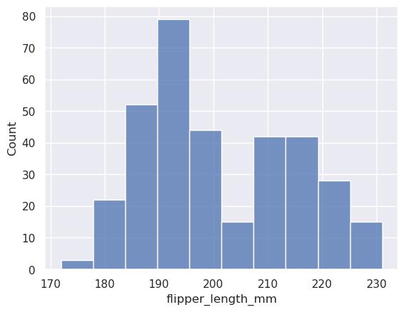
Figure1: Imagegeneratedbytheprovidedcode.
Explanation:
Thehistogramcountshowmanypenguinsfallintoeachbinof flipper_length_mm .Bydefault,Seabornautomaticallychoosesthenumberofbins.
1 sns.histplot(data=penguins, x="flipper_length_mm", bins =30)
2 plt.show()
Changingthenumberofbinsallowsyoutocontrolthegranularityofthehistogram.
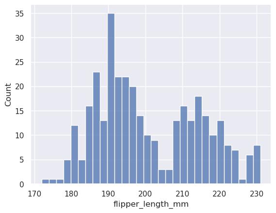
Figure2: Imagegeneratedbytheprovidedcode.
Histogrambycategoryusing hue
1 sns.histplot(data=penguins,
2 x="flipper_length_mm",
3 hue="species",
4 element="step")
5 plt.show()
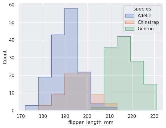
Figure3: Imagegeneratedbytheprovidedcode.
Explanation:
• The hue argumentallowsyoutoseparatethedistributionbyspecies.
• The element="step" makestheplotlessclutteredbydrawingoutlined
histograms.
KDEplotsaresmoothedversionsofhistogramsthathelptoseethedistribution shapemoreclearly.
1 sns.kdeplot(data=penguins, x="flipper_length_mm")
2 plt.show()
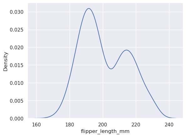
Figure4: Imagegeneratedbytheprovidedcode.
Explanation: Thisshowsasmoothedestimateoftheprobabilitydensityfunction.
KDEbygroupwith hue
1 sns.kdeplot(data=penguins, 2 x="flipper_length_mm", 3 hue="species", 4 fill=True) 5 plt.show()
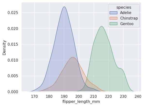
Figure5: Imagegeneratedbytheprovidedcode.
Explanation:
• Byusing hue,youcancomparethedistributionsofflipperlengthsbyspecies.
• fill=True willfilltheareaunderthecurves.
EmpiricalCumulativeDistributionFunctionwith ecdfplot()
AnECDFshowsthecumulativeproportionofthedata.
1 sns.ecdfplot(data=penguins, x="flipper_length_mm")
2 plt.show()
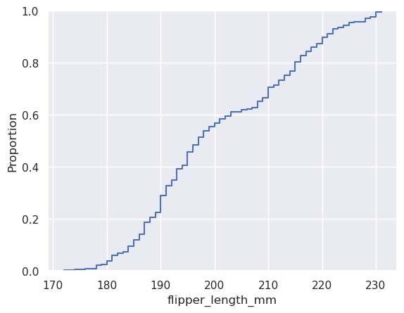
Figure6: Imagegeneratedbytheprovidedcode.
Explanation:
Foreachvalueof flipper_length_mm,theplotshowstheproportionofpenguinswithflipperlengthslessthanorequaltothatvalue.
1 sns.ecdfplot(data=penguins, 2 x="flipper_length_mm",
3 hue="species")
4 plt.show()
Thisvisualizationishelpfulforcomparingdistributionsacrossgroups.
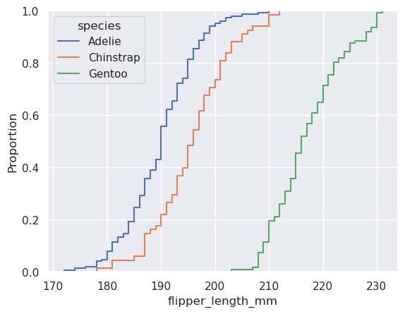
Figure7: Imagegeneratedbytheprovidedcode.
Arugplotaddssmalltickmarksalongtheaxistoshowtheactualdatapoints.
1 sns.rugplot(data=penguins, x="flipper_length_mm")
2 plt.show()
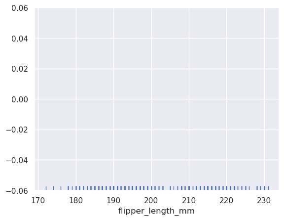
Figure8: Imagegeneratedbytheprovidedcode.
Eachsmallverticallinecorrespondstoadatapoint.Itisusefultovisualizethe densityofdatapoints,especiallywhencombinedwithotherplots.
1 sns.kdeplot(data=penguins, x="flipper_length_mm")
2 sns.rugplot(data=penguins, x="flipper_length_mm")
3 plt.show()
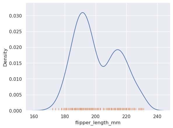
Figure9: Imagegeneratedbytheprovidedcode.
ThecombinationofKDEandrugplotsallowsyoutoseeboththesmootheddistributionandtheactualdatapoints.
• histplot(), kdeplot(),and ecdfplot() acceptcommonarguments like hue, multiple, element, fill,and common_norm.
• Youcaneasilycombinedistributionplotstocreatelayeredvisualizations.
• KDEissensitivetooutliers;useitcarefullywithnoisydata.
histplot() Showfrequencycounts(histogram) kdeplot() Estimateandplotthedistribution’sdensity ecdfplot() Displaycumulativedistributionfunction rugplot() Showindividualdatapointsalonganaxis
Inthenextchapter,wewillexplore CategoricalPlots,whichareessential whenworkingwithqualitativedata.
Categoricalplotsareamongthemostfrequentlyusedtypesofplotsindataanalysis.Theyareessentialforvisualizingtherelationshipbetweencategoricaland numericalvariablesorforcomparingdistributionsacrossdi erentcategories. Seabornprovidesmultiplefunctionstocreatecategoricalplots,eachwithitsown strengths:
• barplot():Estimateanddisplaythemean(orotherestimator)ofanumericalvariableacrosscategories.
• countplot():Displaycountsofobservationsineachcategoricalbin.
• boxplot():Showdistributionswithquartilesandoutliers.
• violinplot():CombineaboxplotandaKDEforricherdistributioninformation.
• stripplot():Displayallindividualdatapoints,usefulforsmalldatasets.
• swarmplot():Displayindividualpointswithoutoverlap.
Inthischapter,wewillexploretheseplotsindepth.
Barplotsareusedtoshowtheaverageofanumericalvariableforeachcategory, o enwithconfidenceintervals.
1 sns.barplot(data=tips, x="day", y="total_bill") 2 plt.show()
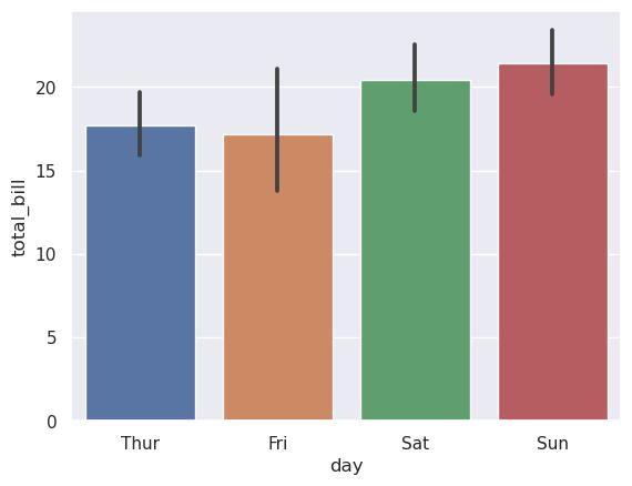
Figure1: Imagegeneratedbytheprovidedcode.
Explanation:
Thisplotshowsthe average total_bill foreachdayoftheweek.
Youcanchangetheestimator(bydefaultisthemean)toothersummarystatistics likethemedian:
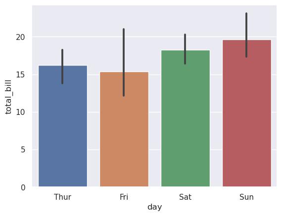
Figure2: Imagegeneratedbytheprovidedcode.
Barplotwith hue
1 sns.barplot(data=tips, 2 x="day", 3 y="total_bill", 4 hue="sex")
5 plt.show()
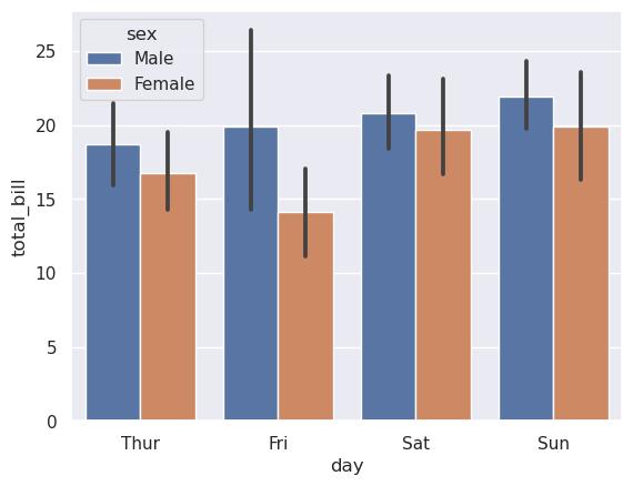
Figure3: Imagegeneratedbytheprovidedcode.
Explanation:
Thebarsaresplitby sex withineachday.
Unlike barplot(), countplot() directlycountsthenumberofobservations ineachcategory.
1 sns.countplot(data=tips, x="day")
2 plt.show()
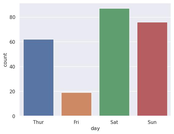
Figure4: Imagegeneratedbytheprovidedcode.
Explanation:
Showshowmanyrecordsthereareforeachdayinthedataset.
Countplotwith hue
1 sns.countplot(data=tips, x="day", hue="sex")
2 plt.show()
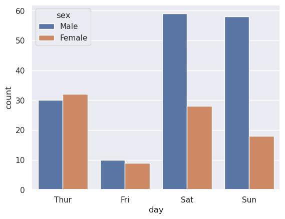
Figure5: Imagegeneratedbytheprovidedcode.
Thisishelpfulforvisualizinghowthecountsvarybetweensubgroups.
Boxplotsshowthedistributionofanumericalvariableusingquartilesandhighlightingpotentialoutliers.
1 sns.boxplot(data=tips, x="day", y="total_bill")
2 plt.show()
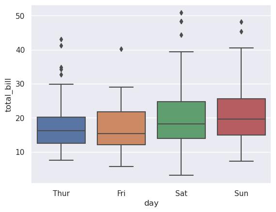
Figure6: Imagegeneratedbytheprovidedcode.
Explanation:
• Theboxrepresentstheinterquartilerange(IQR).
• Thelineinsidetheboxshowsthemedian.
• The“whiskers”extendto1.5*IQR,andpointsbeyondareconsideredoutliers.
Boxplotwith hue
1 sns.boxplot(data=tips, x="day", y="total_bill", hue="sex" )
2 plt.show()
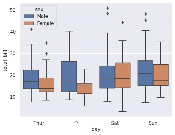
Figure7: Imagegeneratedbytheprovidedcode.
Adding hue allowsustocomparedistributionsbetweensubgroups.
Violinplotscombinetheinformationofaboxplotandakerneldensityestimation (KDE).
Basicviolinplot
1 sns.violinplot(data=tips, x="day", y="total_bill")
2 plt.show()
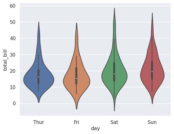
Figure8: Imagegeneratedbytheprovidedcode.
Explanation:
Youcanseethedistributionshapeandquartilessimultaneously.
Violinplotwithsplitandhue
1 sns.violinplot(data=tips, 2 x="day", 3 y="total_bill", 4 hue="sex",
6 plt.show()
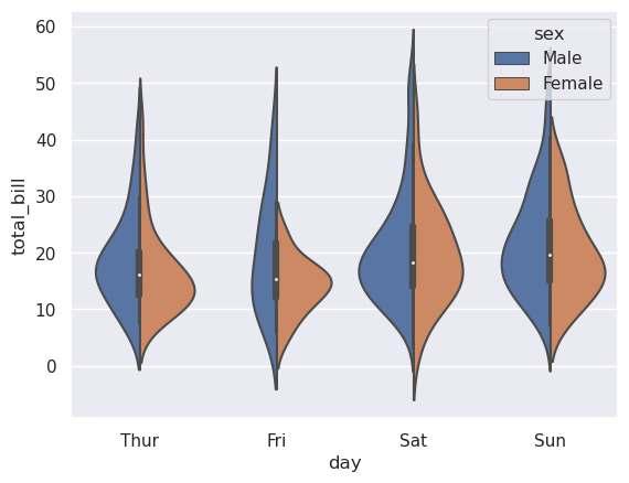
Figure9: Imagegeneratedbytheprovidedcode.
Thisallowsyoutoseebothdistributionsinthesame“violin”when hue hastwo categories.
Stripplotsarescatterplotswherepointsarearrangedalongacategoricalaxis.
1 sns.stripplot(data=tips, x="day", y="total_bill") 2 plt.show()
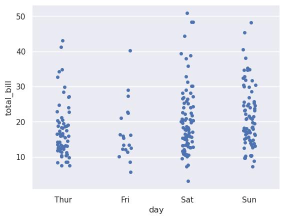
Figure10: Imagegeneratedbytheprovidedcode.
Explanation:
Usefultoseealldatapoints,especiallywithsmalldatasets.
1 sns.stripplot(data=tips, 2 x="day", 3 y="total_bill", 4 jitter=True, 5 hue="sex") 6 plt.show()
• jitter=True spreadsthepointstoavoidoverlap.
• Combiningwith hue helpstodistinguishsubgroups.
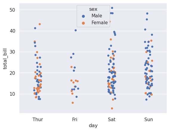
Figure11: Imagegeneratedbytheprovidedcode.
Swarmplotsimproveuponstripplotsbyautomaticallyadjustingpointpositions toavoidoverlaps.
Basicswarmplot
1 sns.swarmplot(data=tips, x="day", y="total_bill")
2 plt.show()
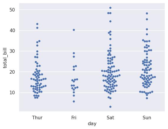
Figure12: Imagegeneratedbytheprovidedcode.
Eachpointrepresentsanobservation,carefullyplacedtoavoidcollisions.
1 sns.swarmplot(data=tips, x="day", y="total_bill", hue=" sex")
2 plt.show()
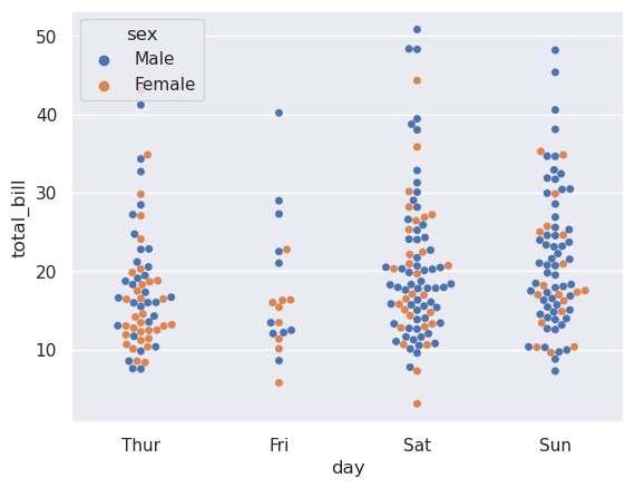
Figure13: Imagegeneratedbytheprovidedcode.
PlotWhentouse
barplot()
countplot()
boxplot()
violinplot()
stripplot()
swarmplot()
Whenyouwanttoshow aggregatedstatistics (mean, median)bycategory
Whenyouwanttoshow counts ofobservationsper category
Whenyouwanttoshow distributionsummary and detect outliers
Whenyouwanttoshow distributionshape and summarystatistics together
Whenyouwanttoshow alldatapoints forsmall datasets
Sameas stripplot() butbetterhandlingof overlappingpoints
• Combiningplotsiscommon: boxplot() + stripplot() or violinplot() + swarmplot() createmoreinformativeplots.
• Bemindfulofreadabilitywhenplottingmanycategories.
• Alwayscheckif hue improvesorcluttersyourvisualization.
Inthenextchapter,wewillexplore RegressionPlots,whichareessential whenyouwanttomodelandvisualizelinearornon-linearrelationships betweenvariables.
Regressionplotsaredesignedtovisualizetherelationshipbetweentwovariables, o entorevealandcommunicatetrendsorpatterns.Theyarecommonlyused to:
• Visualizelinearrelationships.
• Detectnon-linearpatterns.
• Communicatethestrengthofarelationship.
• Showmodel-basedpredictions.
Seabornprovidestwomainfunctionsforregressionplots:
• regplot():Low-levelfunctionthatcreatesascatterplotwitharegression line.
• lmplot():High-levelfunctionwithadditionaloptionsforfacetingandeasy grouping.
Basicregressionplot
1 sns.regplot(data=tips, x="total_bill", y="tip")
2 plt.show()

Figure1: Imagegeneratedbytheprovidedcode.
Explanation:
Thisplotshowsascatterplotof total_bill vs tip withafittedlinearregression lineanda95%confidenceintervalbydefault.
Removingtheconfidenceinterval(ci=None)
1 sns.regplot(data=tips, x="total_bill", y="tip", ci=None)
2 plt.show()
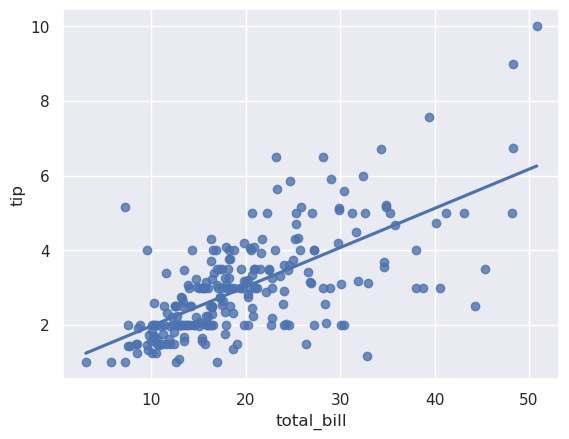
Figure2: Imagegeneratedbytheprovidedcode.
Thissimplifiestheplotbyremovingtheshadedconfidenceinterval.
Bydefault,Seabornfitsalinearmodel,butyoucanfithigher-orderpolynomials.
1 sns.regplot(data=tips, x="total_bill", y="tip", order=2)
IbonMartínez-ArranzPage53
2 plt.show()
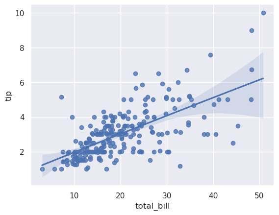
Figure3: Imagegeneratedbytheprovidedcode.
Explanation:
The order=2 argumentfitsaquadraticregressionline.
Robustregression
Youcanmaketheregressionrobusttooutliersbyusing robust=True.
1 sns.regplot(data=tips, x="total_bill", y="tip", robust= True)
2 plt.show()
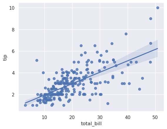
Figure4: Imagegeneratedbytheprovidedcode.
Unlike regplot(), lmplot() allowseasygroupingandfaceting.
1 sns.lmplot(data=tips, x="total_bill", y="tip") 2 plt.show()
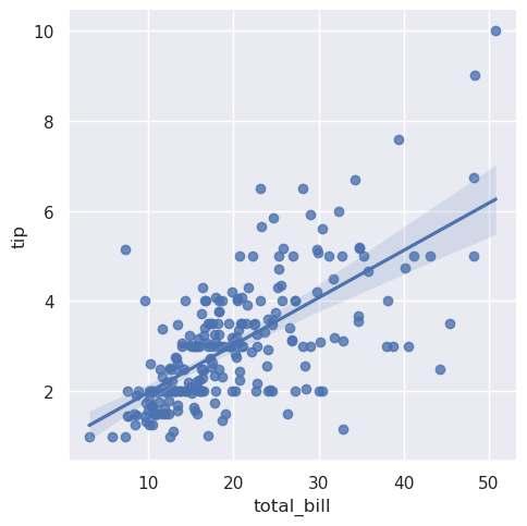
Figure5: Imagegeneratedbytheprovidedcode.
Producesthesameresultas regplot() butreturnsaFacetGridobject.
Regressionwith hue
1 sns.lmplot(data=tips, x="total_bill", y="tip", hue="sex") 2 plt.show()
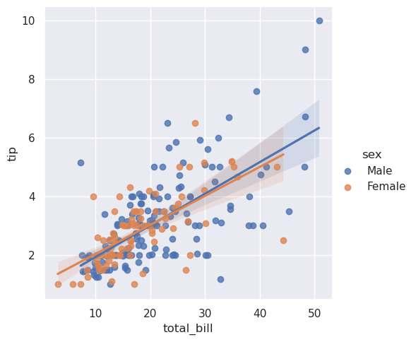
Figure6: Imagegeneratedbytheprovidedcode.
Eachgroup(sex)hasitsownregressionlineandscatterpoints.
1 sns.lmplot(data=tips, 2 x="total_bill",
3 y="tip", 4 hue="sex", 5 markers=["o", "s"]) 6 plt.show()
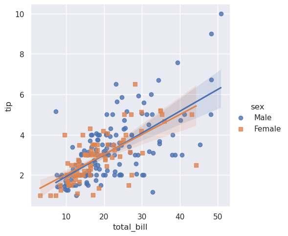
Figure7: Imagegeneratedbytheprovidedcode.
Youcanassigndi erentmarkerstoeachgroupforbetterreadability.
Facetingwith col and row
1 sns.lmplot(data=tips,
y="tip",
col="sex",
row="smoker")
plt.show()
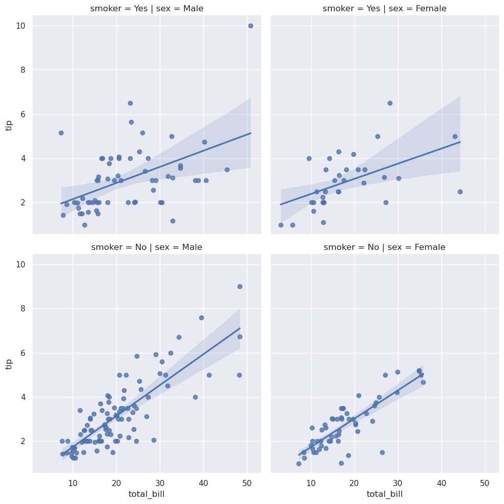
Figure8: Imagegeneratedbytheprovidedcode.
Explanation:
Thisisapowerfulfeature:youcansplitthedataintomultiplepanelsbycategories.
Seaborndoesnotdirectlysupportmultipleregressioninthestatisticalsense(with multiple x variables),butyoucanstill:
1.Splitdatausing hue tosimulategroup-wisemultipleregression.
2.Usecolor,size,orstyletoshowadditionalinformation.
1 sns.lmplot(
2 data=tips,
3 x="total_bill",
4 y="tip",
5 hue="sex",
6 col="smoker",
7 scatter_kws={"s":50},
8 line_kws={"linewidth":2}
9 )
10 plt.show()
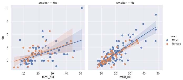
Figure9: Imagegeneratedbytheprovidedcode.
Explanation:
Thisplotcomparesregressionlinesbyboth sex and smoker status,givinginsight intothecombinede ect.
ArgumentsSummary
ArgumentDescription
order
Polynomialregressionorder ci
hue
Confidenceinterval(default95%)
Groupbyacategoricalvariable robust
Robustregressiontoreduceoutlierinfluence markers
Specifymarkerstyle(s)
ArgumentDescription
col / row
scatter_kws
line_kws
Facetingbycategories(lmplotonly)
Customizescatterplotaesthetics
Customizeregressionlineaesthetics
FunctionRecommendedfor
regplot()
lmplot()
Simpleregressionplotswithoutgroupingor faceting
Regressionplotsinvolvinggrouping(hue)or faceting(col, row)
Notes
• Alwayscheckifalinearmodelisappropriate.Inmanyreal-worldcases, relationshipsmaybenon-linear.
• Robustregressionishelpfulwhenyoususpectoutliersarea ectingthe model.
• Avoidoverfittingwhenincreasing order forpolynomialregressions.
Inthenextchapter,wewillexplore MatrixandHeatmapPlots,which areidealforvisualizingrelationshipsbetweenmanyvariables,especially correlations.
Matrixplotsareessentialforvisualizing structureddata suchas:
• Correlationmatrices
• Distancematrices
• Contingencytables
• Anytwo-dimensionalarrayofvalues
Seaborno erstwomainfunctionsformatrixvisualizations:
• heatmap():Displaysamatrixwithcoloredcells,optionallyannotated.
• clustermap():Extends heatmap() byapplyingclustering(hierarchical) torowsand/orcolumnsautomatically.
Theseplotsarecommonlyusedtoidentifypatterns,clusters,orstrongrelationships betweenvariables.
Atypicaluseofmatrixplotsistovisualizethe correlation betweennumerical variables.
Let’susethe penguins dataset:
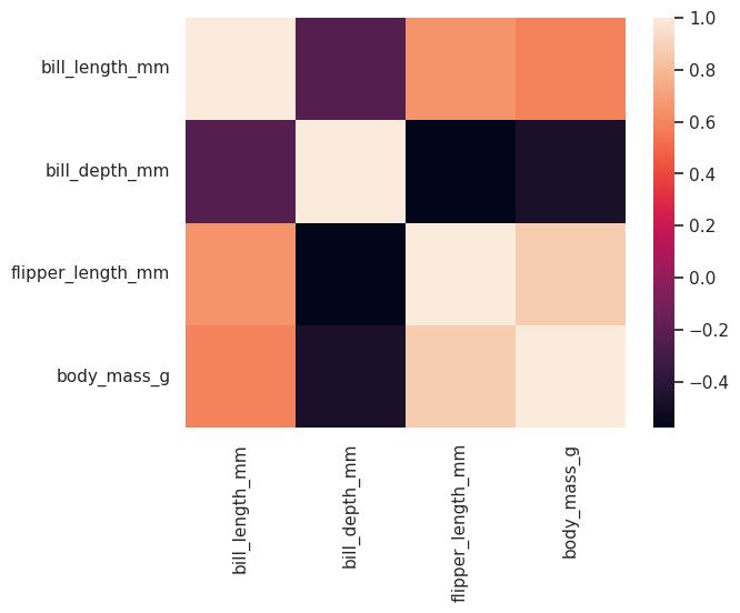
Figure1: Imagegeneratedbytheprovidedcode.
Explanation:
• Darkercolorsrepresentstrongercorrelations.
• Bydefault,Seabornusesabluecolorpalette.
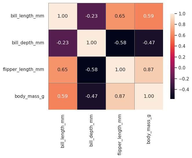
1 sns.heatmap(corr, annot=True)
2 plt.show()

Figure2: Imagegeneratedbytheprovidedcode.
Explanation:
annot=True displaysthecorrelationcoe icientinsideeachcell.
1 sns.heatmap(corr, annot=True, cmap="coolwarm", center=0) 2 plt.show()
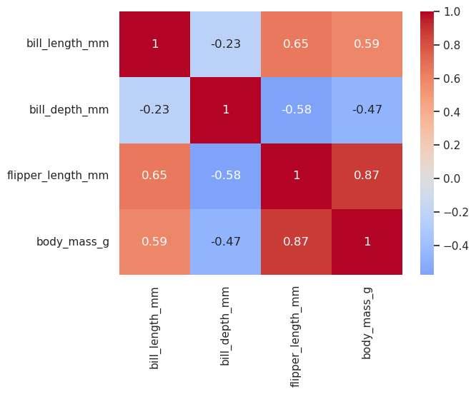
Figure3: Imagegeneratedbytheprovidedcode.
Explanation:
• cmap="coolwarm" helpshighlightpositiveandnegativecorrelations.
• center=0 ensuresthatthecolormapissymmetricaroundzero.
• fmt=".2f" formatsnumberswithtwodecimals.
• linewidths and linecolor addgridlinesbetweencells.
• cbar_kws adjuststhecolorbarsize.
clustermap() performshierarchicalclusteringofrowsandcolumnstoreveal structuresandgroupsinthedata.
1 sns.clustermap(corr) 2 plt.show()
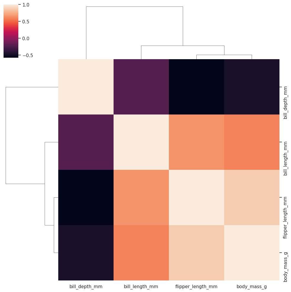
Figure5: Imagegeneratedbytheprovidedcode.
Explanation:
• Variablesarereorderedtoshowclusters.
• Dendrogramsaredisplayedtorepresentthehierarchicalclustering.
1 sns.clustermap(corr, 2 cmap="coolwarm", 3 annot=True, 4 fmt=".2f", 5 linewidths=0.5)
6 plt.show()
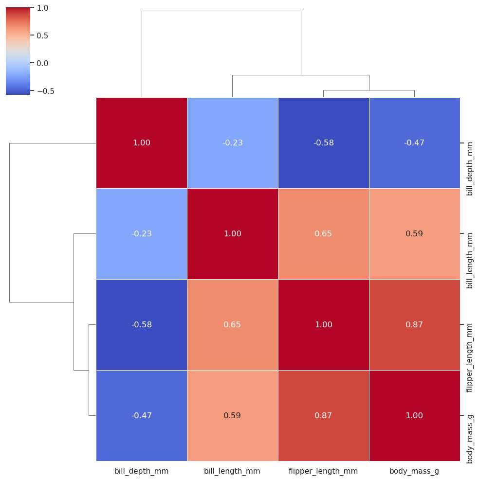
Figure6: Imagegeneratedbytheprovidedcode.
Explanation:
Youcanpassmostargumentsfrom heatmap() to clustermap().
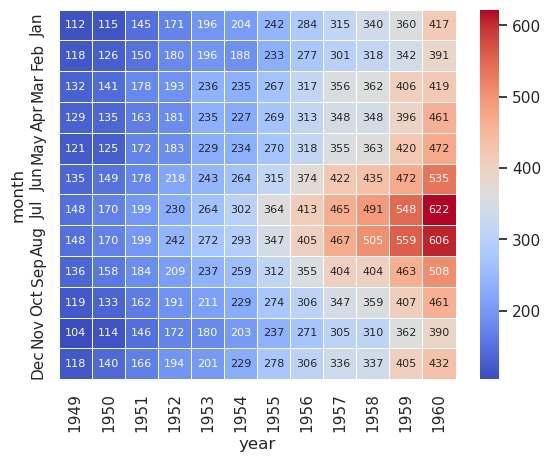
• Rowsaremonths,columnsareyears,andthevaluesrepresentthenumber ofpassengers.
• Thisisaperfectexampleofa timematrix.
1 sns.clustermap(flights_pivot, cmap="coolwarm") 2 plt.show()
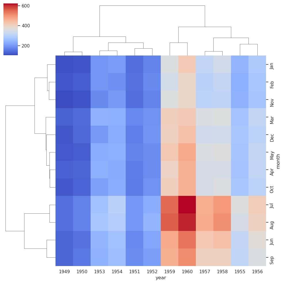
Figure8: Imagegeneratedbytheprovidedcode.
Explanation:
Thisautomaticallyclustersbothmonthsandyearsbasedonthenumberofpassengers,revealingpatternssuchassimilaryearsorseasonalclusters.
• heatmap() isgreatfor knownmatrices,likecorrelations.
• clustermap() ishelpfulwhenyoususpectthedatamighthave hidden structure.
• Adjustthe cmap tohighlightthetypeofinformationyouwanttoemphasize (diverging,sequential,etc.).
• Alwayslabelyouraxesclearlywhenreshapingdata.
heatmap()
clustermap()
Plotanynumericmatrixwith customizablecolorsandannotations
Plotamatrixwithhierarchical clusteringappliedautomatically
annot=True Displaynumericalvaluesinsidethe cells
cmap= Controlthecolorpalette fmt= Controlthenumberformattingin annotations
Inthenextchapter,wewilllearnhowtouse FacetGridandPairGrid,two essentialtoolsforbuildingcomplexgridsofplotsautomatically.
OneofSeaborn’sstrengthsisitsabilitytoeasilycreate multi-plotgrids,allowing youto:
• Exploredistributionsorrelationshipsacrosssubgroups.
• Createpanelplotswithsharedorindependentaxes.
• Automatecomplexplottinglayouts.
Seabornprovidesthreemaintoolsforthis:
• FacetGrid():Themostflexiblewaytocreatecustomgridsofplots.
• pairplot():Aquickwaytovisualizepairwiserelationshipsbetweenvariables.
• catplot():Combinescategoricalplotswithfacetingcapabilities.
1 g = sns.FacetGrid(tips, col="sex")
2 g.map(sns.histplot, "total_bill")
3 plt.show()
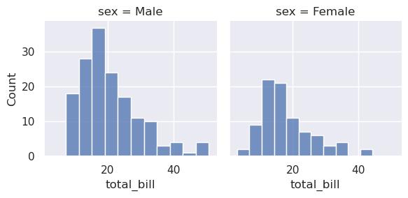
Figure1: Imagegeneratedbytheprovidedcode.
Explanation:
• Createsonehistogramforeachvalueof sex.
• map() allowsyoutospecifytheplottingfunctiontoapply.
1 g = sns.FacetGrid(tips, col="sex", row="smoker")
2 g.map(sns.scatterplot, "total_bill", "tip")
3 plt.show()
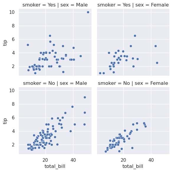
Figure2: Imagegeneratedbytheprovidedcode.
Explanation:
• Createsa gridofscatterplots combining sex and smoker.
• Eachcellofthegridcorrespondstoasubgroup.
1 g = sns.FacetGrid(tips, col="day", hue="sex")
2 g.map(sns.scatterplot, "total_bill", "tip").add_legend()
3 plt.show()
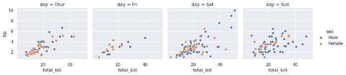
Figure3: Imagegeneratedbytheprovidedcode.
Explanation:
• hue stillworksinsideeachfacet,makingcomparisonseasier.
1 g = sns.FacetGrid(tips, col="day", height=4, aspect=0.7)
2 g.map_dataframe(sns.regplot,
3 x="total_bill", 4 y="tip",
5 scatter_kws={"s":30},
6 line_kws={"color": "red"})
7 g.add_legend()
8 plt.show()
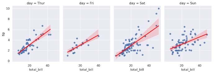
Figure4: Imagegeneratedbytheprovidedcode.
Pairplot
The pairplot() functionisa quickandpowerful waytocreatescatterplot matrices.
BasicPairplot
1 sns.pairplot(penguins.dropna())
2 plt.show()
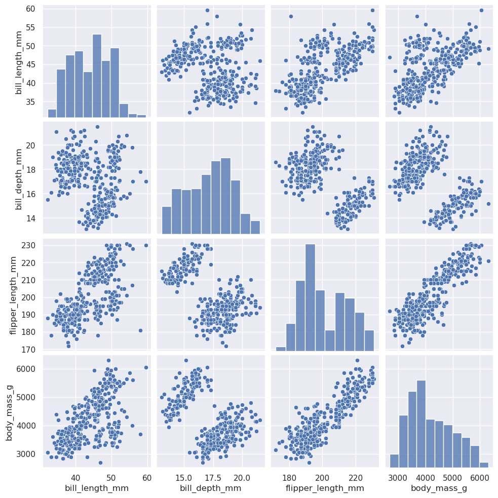
Figure5: Imagegeneratedbytheprovidedcode.
Explanation:
• Automaticallyplotspairwiserelationshipsbetweenallnumericvariables.
• Diagonalplotsshowthedistributionofeachvariable.
Pairplotwith hue
1 sns.pairplot(penguins.dropna(), hue="species") 2 plt.show()
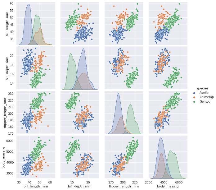
Figure6: Imagegeneratedbytheprovidedcode.
Explanation:
• Colorstheplotsbyspecies.
IbonMartínez-ArranzPage87
• Veryhelpfulfordetectingclustersandpatterns.
1 sns.pairplot(penguins.dropna(),
2 hue="species",
3 markers=["o", "s", "D"])
4 plt.show()
Youcanspecifycustommarkersforeachgroup.
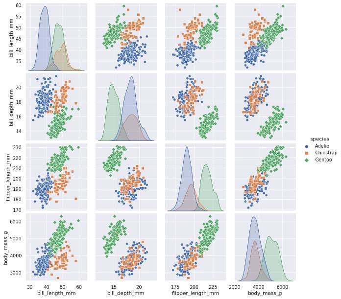
Figure7: Imagegeneratedbytheprovidedcode.
1 sns.pairplot(penguins.dropna(), hue="species", kind="reg" )
2 plt.show()
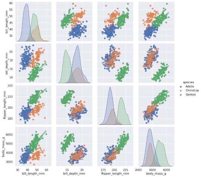
Figure1: Imagegeneratedbytheprovidedcode.
Explanation:
• Addsregressionlinestoscatterplotsinsteadofplainpoints.
catplot() isa general-purpose functionforcategoricalplotswithfacetingbuiltin.
Basiccatplot(equivalenttobarplot)
1 sns.catplot(data=tips, x="day", y="total_bill", kind="bar ")
2 plt.show()
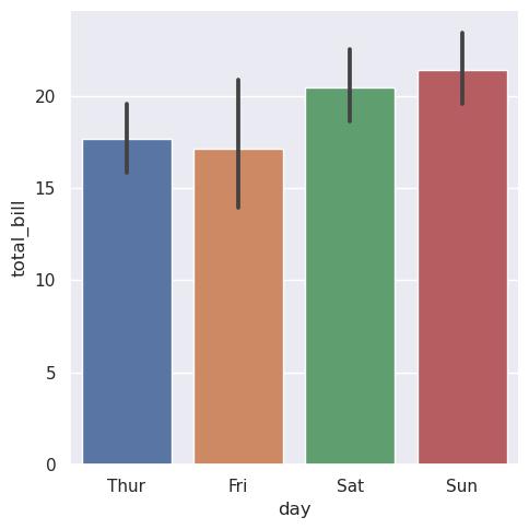
Figure2: Imagegeneratedbytheprovidedcode.
Changingplottype
1 sns.catplot(data=tips, x="day", y="total_bill", kind="box ")
2 plt.show()
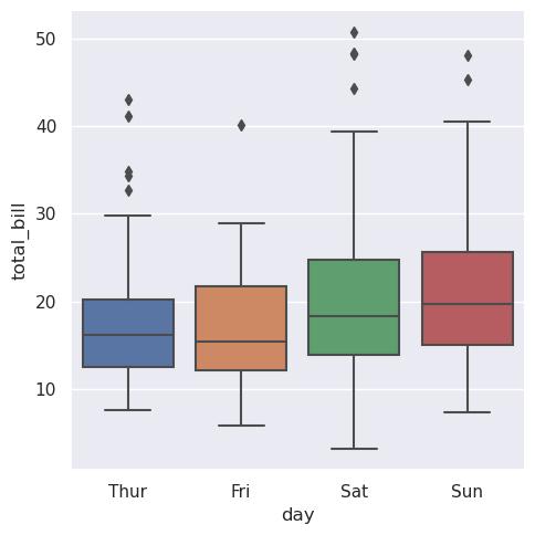
Figure3: Imagegeneratedbytheprovidedcode.
Youcanswitchbetween box, violin, strip, swarm,and bar justbychanging the kind.
Facetingwithcatplot
1 sns.catplot(data=tips, 2 x="day", y="total_bill", 3 hue="sex", 4 col="smoker", kind="box") 5 plt.show()
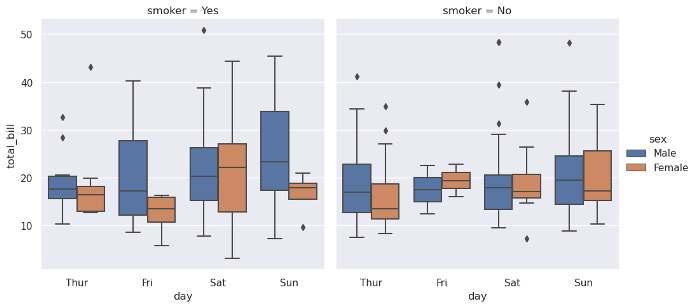
Figure4: Imagegeneratedbytheprovidedcode.
Explanation:
• Createsagridofboxplotssplitby smoker.
• Insideeachplot,the hue separatesthedataby sex.
1 sns.catplot(data=tips, 2 y="day", x="total_bill", 3 kind="violin", hue="sex", split=True) 4 plt.show()
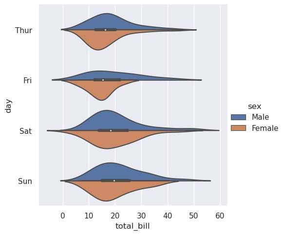
Figure5: Imagegeneratedbytheprovidedcode.
Byswitching x and y,youchangetheorientationoftheplot.
• FacetGrid() givesyoufullcontrolbutrequiresmoremanualsetup.
• pairplot() isexcellentforexploratorydataanalysiswithnumericalvariables.
• catplot() isveryflexibleforcategoricaldataandiso entheeasiestchoice forfast,publication-readyplots.
• Use height and aspect toadjustthesizeoffacets.
• Alwayscheckiftoomanyfacetsmaketheplothardertointerpret.
FacetGrid() Fullcontrolforcreatingcustomgrid plots
pairplot() Automaticpairwisescatterplotsfor numericalvariables
catplot() Categoricalplots+automaticfaceting
Inthenextchapter,wewillfocuson AdvancedCustomization,whereyou willlearnhowtochangethemes,palettes,andstylestomakeyourplots publication-quality.
OneofthegreateststrengthsofSeabornisthatitnotonlymakesiteasytogenerate statisticalplotsbutalsoprovidestoolstomakethem visuallyattractiveand publication-ready.
Inthischapter,youwilllearnhowto:-Changeplotthemesandstyles.-Customize colorpalettes.-Adjustcontextstomatchdi erentaudiences(notebooks,papers, presentations).-Combinealltheseoptionsforfullycustomizedvisualizations.
Seaborncomeswithseveralbuilt-inthemesyoucanusetoquicklyadjustthe overallappearanceofyourplots.
Availablethemes:
• "darkgrid" (default)
• "whitegrid"
• "dark"
• "white"
• "ticks"
1 sns.set_theme(style="whitegrid")
2 sns.boxplot(data=tips, x="day", y="total_bill")
3 plt.show()
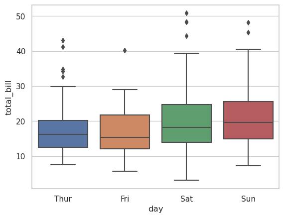
Figure1: Imagegeneratedbytheprovidedcode.
Explanation: whitegrid iscommonlyusedinscientificpublicationsasitprovidescleargridlines.
Ifyouwantmorecontrol,youcanadjustspecificstyleelements.
Example:
1 sns.set_style("whitegrid")
2 sns.set_context("talk", font_scale=1.2)
3 sns.boxplot(data=tips, x="day", y="total_bill")
4 plt.show()
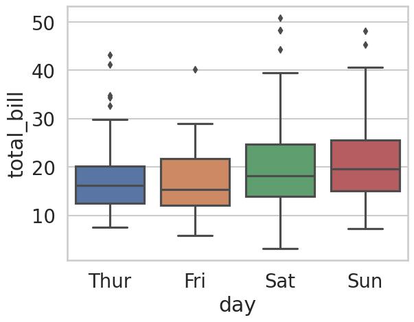
Figure2: Imagegeneratedbytheprovidedcode.
• set_context("talk") adaptstheplotforpresentations.
• font_scale allowsyoutoadjustthesizeoftextelementsglobally.
Colorsplayacrucialroleindatavisualization.Seabornprovidespredefinedpalettes andalsoallowsyoutocreatecustomones.
1 sns.set_theme()
2 sns.boxplot(data=tips, x="day", y="total_bill", hue="sex" )
3 plt.show()
Figure3: Imagegeneratedbytheprovidedcode.
1 sns.set_palette("pastel")
2 sns.boxplot(data=tips, x="day", y="total_bill", hue="sex" )
3 plt.show()
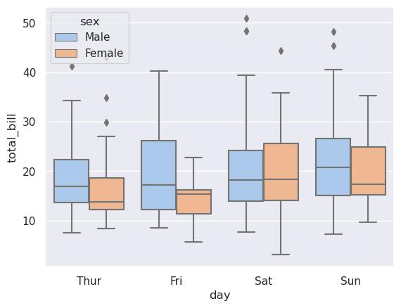
Figure4: Imagegeneratedbytheprovidedcode.
Example:Usingasequentialpalette
1 sns.set_palette("Blues")
2 sns.violinplot(data=tips, 3 x="day", y="total_bill", 4 hue="sex", split=True) 5 plt.show()
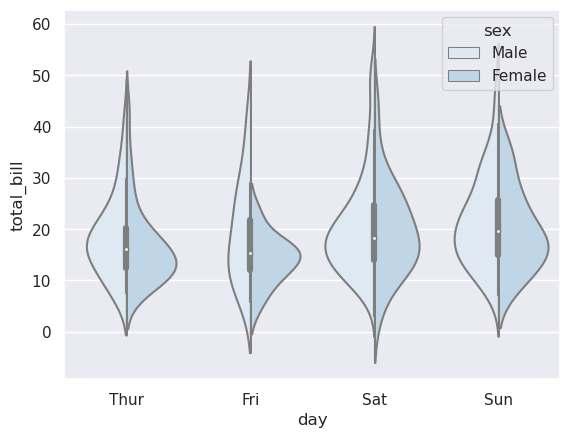
Figure5: Imagegeneratedbytheprovidedcode.
1 custom_palette =["#FF6F61", "#6B5B95"]
2 sns.set_palette(custom_palette)
3 sns.barplot(data=tips, x="day", y="total_bill", hue="sex" )
4 plt.show()
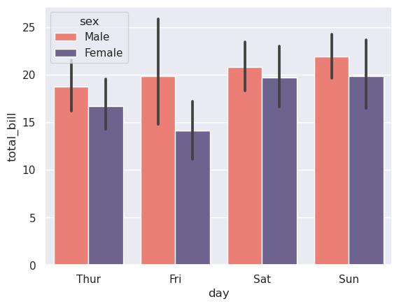
Figure6: Imagegeneratedbytheprovidedcode.
Seabornallowsyoutoadjustthe scale ofelementsdependingonyourtarget audience.
Availablecontexts:
• "paper" (smallerplotsforpapers)
• "notebook" (default)
• "talk" (suitableforpresentations)
• "poster" (forlargevisuals)
1 sns.set_context("poster")
2 sns.barplot(data=tips, x="day", y="total_bill", hue="sex" )
3 plt.show()
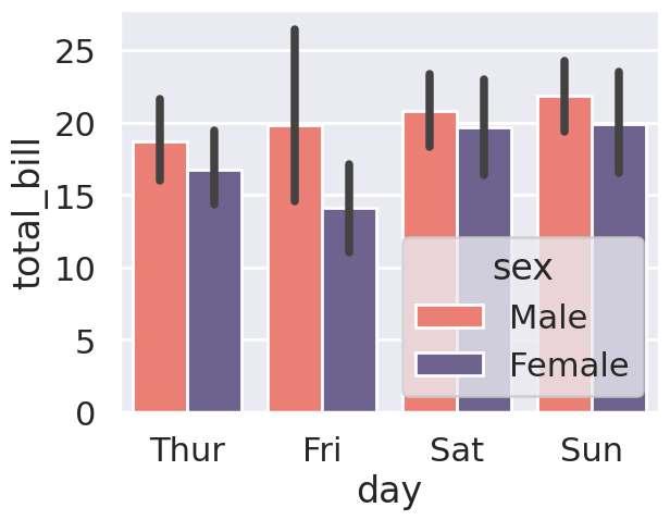
Figure7: Imagegeneratedbytheprovidedcode.
Noticehowallelements(text,lines,markers)arelarger,suitableforprojecting slidesorposters.
1 sns.set_theme(style="ticks", 2 palette="Set2", 3 context="talk")
4 sns.violinplot(data=tips, 5 x="day", y="total_bill", hue="sex", 6 split=True)
7 plt.show()
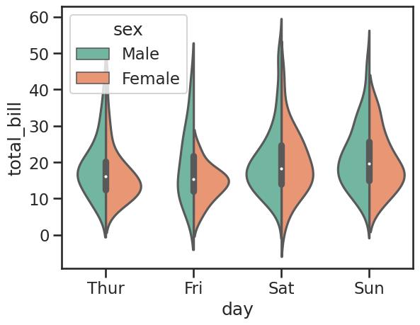
Figure8: Imagegeneratedbytheprovidedcode.
Bycombiningstyle,palette,andcontext,youcancreatecustomizedplotsadapted toyourspecificneeds.
Youcanapplytemporarychangestoaspecificplotwithouta ectingothers:
1 withsns.axes_style("whitegrid"):
2 sns.boxplot(data=tips, x="day", y="total_bill")
3 plt.show()
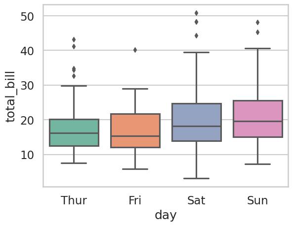
Figure9: Imagegeneratedbytheprovidedcode.
Thisishelpfulwhenyouwanttoapplyadi erentstyleforaspecificplotwithout alteringtheglobaltheme.
SummaryTable FunctionPurpose
set_theme() Settheoverallstyleandpalette
set_style() Changethebackgroundandgrid appearance set_palette() Chooseordefinecolorpalettes set_context() Adjustplotsizeandelementsfor di erentoutputs withsns.axes_style() Temporarilyapplyastylefora specificplot
• For papers:use style="whitegrid", context="paper",and sequentialordivergingpalettes.
• For notebooks: style="darkgrid" and context="notebook" work wellforquickexplorations.
• For presentations:increase font_scale anduse context="talk" or "poster".
• Choosepalettesthatare:
– Colorblind-friendly.
– Consistentwiththestoryyouwanttotell.
– Notoverloadedwithtoomanycolors.
Inthenextchapter,youwilllearnhowtoadd AnnotationsandDetails to makeyourplotsmoreinformativeandvisuallyappealing.
Annotationsandsmalldetailso enmakethedi erencebetweenasimpleplotand agreatplot.Theyallowyouto:
• Highlightimportantfindings.
• Improvereadability.
• Guidetheviewertothekeymessages.
• Makeplotssuitableforpresentationsandpublications.
Inthischapter,youwilllearnhowto:
• Customizeaxislabels,titles,legends.
• Addtextannotationsandmarkers.
• Drawreferencelines.
• Controlticksandgridappearance.
SeabornintegratessmoothlywithMatplotlib,soyoucaneasilyadjustthebasic componentsofyourplots.
1 sns.scatterplot(data=tips, x="total_bill", y="tip")
2 plt.title("TipsvsTotalBill")
3 plt.xlabel("TotalBill($)")
4 plt.ylabel("Tip($)")
5 plt.show()
Explanation:
Alwayslabelyouraxesandgiveyourplotacleartitle.
1 sns.scatterplot(data=tips, 2 x="total_bill", y="tip", hue="sex")
3 plt.legend(title="Gender", loc="upperleft")
4 plt.show()
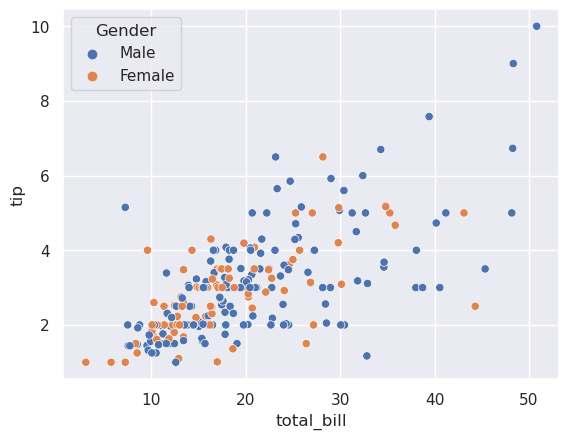
Figure1: Imagegeneratedbytheprovidedcode.
Explanation:
Youcancontrolthelegendpositionandtitleusing plt.legend().
AddingTextAnnotations
Youcanuse plt.text() toinserttextanywhereinyourplot.
Example:
1 sns.scatterplot(data=tips, x="total_bill", y="tip")
2 plt.text(40,8, "Hightiphere!", fontsize=12, color="red ")
3 plt.show()
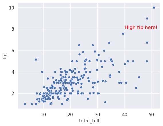
Figure2: Imagegeneratedbytheprovidedcode.
Explanation:
Useannotationstohighlightspecificpointsorregions.
Youcanalsoplotspecificpointswithdi erentaesthetics.
Example:
1 sns.scatterplot(data=tips, x="total_bill", y="tip")
2 plt.scatter(7.4,5.15, s=200,
3 facecolors='none' ,
4 edgecolors='red' ,
5 linewidths=2)
6 plt.text(7.4,5.65, "Outlier?", color="red")
7 plt.show()
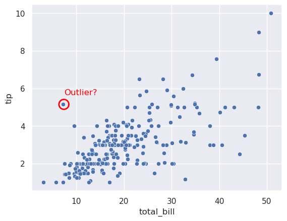
Figure3: Imagegeneratedbytheprovidedcode.
Explanation:
Thistechniqueiso enusedtopointoutoutliersorinterestingdatapoints.
1 sns.scatterplot(data=tips, x="total_bill", y="tip")
2 plt.axhline(5, linestyle="--", color="gray")
3 plt.axvline(30, linestyle="--", color="gray")
4 plt.show()
• axhline() drawsahorizontalline.
• axvline() drawsaverticalline.
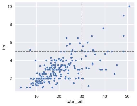
Figure4: Imagegeneratedbytheprovidedcode. Diagonalorcustomlineswith plot()
1 sns.scatterplot(data=tips, x="total_bill", y="tip")
2 plt.plot([0,50],[0,10], linestyle="--", color="purple" )
3 plt.show()
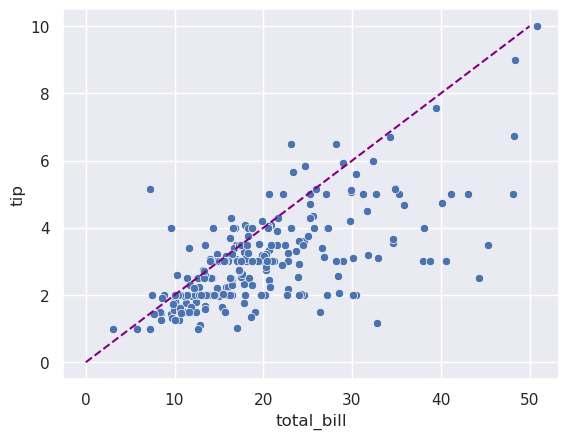
Figure5: Imagegeneratedbytheprovidedcode.
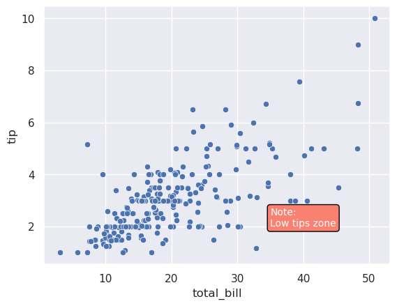
Youcancreatetextwithbackgroundusing bbox.
1 sns.scatterplot(data=tips, x="total_bill", y="tip")
2 plt.text(35,2, "Note:\nLowtipszone",
3 fontsize=10,
1 sns.scatterplot(data=tips, x="total_bill", y="tip")
2 plt.xticks([10,20,30,40,50])
3 plt.yticks([2,4,6,8,10])
4 plt.show()
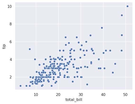
Figure7: Imagegeneratedbytheprovidedcode.
Adjustinggrid
1 sns.set_style("whitegrid")
2 sns.scatterplot(data=tips, x="total_bill", y="tip")
3 plt.grid(True, linestyle="--", linewidth=0.5)
4 plt.show() Page122IbonMartínez-Arranz
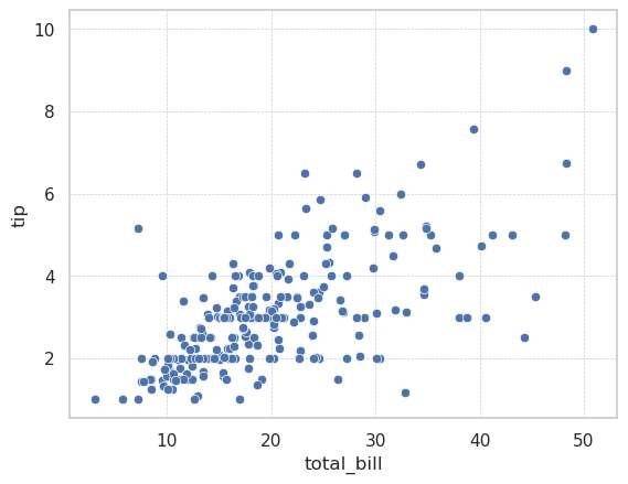
Figure8: Imagegeneratedbytheprovidedcode.
1 sns.scatterplot(data=tips, 2 x="total_bill", y="tip", hue="sex")
3 plt.title("TipsvsTotalBillbyGender")
4 plt.xlabel("TotalBill($)")
5 plt.ylabel("Tip($)")
6 plt.axhline(5, linestyle="--", color="gray")
7 plt.axvline(30, linestyle="--", color="gray")
8 plt.text(40,8, "Hightipzone", fontsize=12, color="red" )
9 plt.legend(title="Gender", loc="upperleft")
10 plt.grid(True, linestyle="--", linewidth=0.5)
11 plt.show()
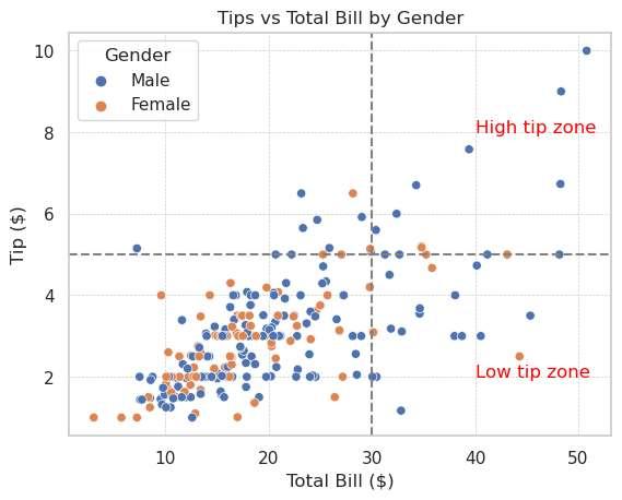
Figure9: Imagegeneratedbytheprovidedcode. Thisexampleputstogetheralltheconceptscoveredinthischapter.
plt.title(), plt.xlabel(), plt.ylabel()
Setplottitleandaxislabels
plt.legend() Customizelegend
plt.text()
Addtextannotations
plt.scatter() Highlightspecificpoints
plt.axhline(), plt.axvline()
plt.grid()
plt.xticks(), plt.yticks()
Addreferencelines
Controlgridappearance
Customizetickmarks
Inthenextchapter,wewilllearnhowtointegrate SeabornwithMatplotlib, givingyoufullcontroloveryourfigureswhenyouneedadvancedcustomizations.
Throughoutthisbook,wehavefocusedonusingSeaborntocreatebeautifuland informativevisualizations.OneofthegreatadvantagesofSeabornisthatitisbuilt ontopofMatplotlib,whichmeansyouareneverlimitedtoSeaborn’sdefault functionality.Infact,combiningSeabornandMatplotlibisthekeytoproducing fullycustomizedplots.
WhileSeabornprovideshigh-levelplottingfunctionswithsmartdefaultsandeasyto-useinterfaces,Matplotlibgivesyou low-levelaccess to:
• Fine-tunethelayoutanddesignofyourplots.
• Controlelementslikeaxes,legends,annotations,andtickmarks.
• Buildcomplexfigurecompositions(e.g.,custommulti-panellayouts).
Inotherwords, Seabornmakesiteasytocreatebeautifulstatisticalplots,and Matplotliballowsyoutomakethemexactlythewayyouwant.
Inthischapter,youwilllearnhowto:
• AccessandmanipulatetheunderlyingMatplotlibaxesandfiguresfrom Seabornplots.
• Combinemultipleplotsintocustomlayouts.
• Addannotations,arrows,referencelines,andotherfinedetails.
• Controllegendplacementandfiguresizesfordi erentusecases.
Masteringthiscombinationwillgiveyoufullcontroloveryourvisualizations, whetheryouarepreparing:
• Aquickexploratoryplot.
• Areportfigure.
• Aslideforapresentation.
• Apublication-qualityfigure.
Let’snowexplorehowSeabornandMatplotlibworktogetherseamlessly.
1 ax = sns.scatterplot(data=tips, x="total_bill", y="tip")
2 ax.set_title("ScatterplotwithMatplotlibTitle")
3 ax.set_xlabel("TotalBill($)")
4 ax.set_ylabel("Tip($)")
5 plt.show()
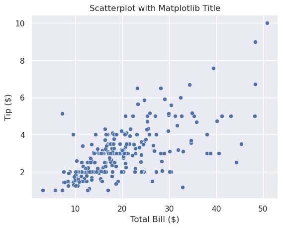
Figure1: Imagegeneratedbytheprovidedcode.
Explanation:
• Seabornreturnsthe AxesSubplot objectdirectly.
• Youcanuse set_title(), set_xlabel(), set_ylabel() asyou wouldinpureMatplotlib.
1 ax = sns.boxplot(data=tips, x="day", y="total_bill")
2 ax.set_xticklabels(["Thu", "Fri", "Sat", "Sun"], rotation =45)
3 plt.show()
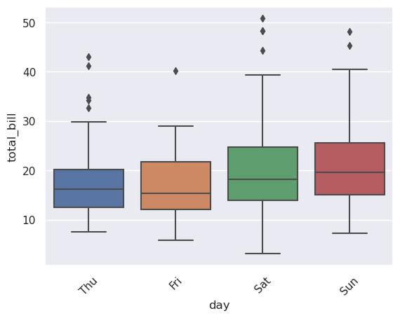
Figure2: Imagegeneratedbytheprovidedcode.
Explanation:
CustomizeticklabelsjustlikeinMatplotlib.
Whenusingmultipleplots,itiscommontoadjustspacingmanually.
1 fig, axes = plt.subplots(1,2, figsize=(10,4))
2
3 sns.histplot(data=tips, x="total_bill", ax=axes[0])
4 sns.boxplot(data=tips, x="day", y="total_bill", ax=axes [1])
5
6 plt.tight_layout()
7 plt.show()
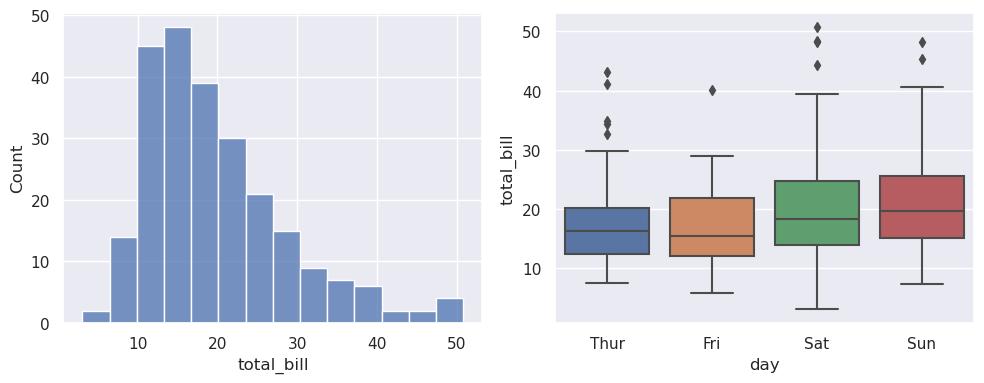
Figure3: Imagegeneratedbytheprovidedcode.
Explanation:
• plt.subplots() createsmultipleMatplotlibaxes.
• Passeach ax toSeaborn’s ax= argument.
• tight_layout() improvesspacingautomatically.
1 fig, axes = plt.subplots(2,2, figsize=(12,8))
3 sns.histplot(data=tips, 4 x="total_bill", 5 ax=axes[0,0])
6 sns.boxplot(data=tips, 7 x="day", y="total_bill", 8 ax=axes[0,1])
9 sns.scatterplot(data=tips, 10 x="total_bill", y="tip", hue="sex", 11 ax=axes[1,0])
12 sns.violinplot(data=tips, 13 x="day", y="total_bill", hue="sex", 14 split=True, ax=axes[1,1])
16 plt.tight_layout() 17 plt.show()
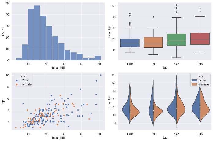
Figure4: Imagegeneratedbytheprovidedcode.
Thisisextremelyusefulfor:
• Creatingcustommulti-plotlayouts.
• Preparingfiguresforpapersandreports.
CombiningSeabornandMatplotlibElements
YoucanaddMatplotlibannotations,arrows,andshapesontopofSeabornplots.
1 ax = sns.scatterplot(data=tips, x="total_bill", y="tip")
2
3 #AddMatplotlibelements
4 ax.axhline(5, linestyle="--", color="red") IbonMartínez-ArranzPage133
5 ax.text(40,8, "Hightipszone", fontsize=12, color="red" )
6 ax.annotate("Outlier?",
xy=(7.4,5.15),
xytext=(8.9,6.65),
arrowprops=dict(facecolor='black' ,
arrowstyle="->"))
plt.show()
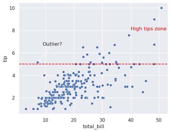
Figure5: Imagegeneratedbytheprovidedcode.
• axhline(), text(), annotate() arefromMatplotlibbutworkseamlesslyonSeabornaxes.
1 ax = sns.scatterplot(data=tips,
2 x="total_bill", y="tip", hue="sex")
3 ax.legend(loc="centerleft", bbox_to_anchor=(1,0.5))
4 plt.tight_layout()
5 plt.show()
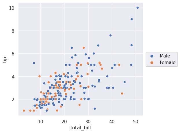
Figure6: Imagegeneratedbytheprovidedcode.
Thisiso ennecessarywhenplotsaretightorwhenpreparingfiguresforpapers.
AlthoughSeabornautomaticallyadaptstofiguresize,youmaywantfullcontrol.
Example:
1 plt.figure(figsize=(8,6))
2 sns.boxplot(data=tips, x="day", y="total_bill")
3 plt.show()
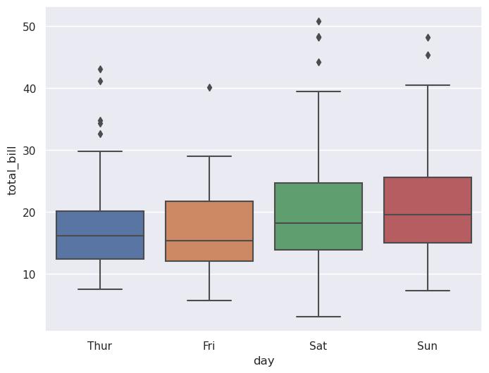
Figure7: Imagegeneratedbytheprovidedcode.
Alternatively,use subplots() andcontrolindividualaxessizesifneeded.
• UseSeabornforplottingandMatplotlibfor fine-tuning.
• plt.subplots() + ax=axes[...] givesyoufullcontroloverlayouts.
• YoucanfreelycombineMatplotlibelementslikearrows,text,annotations withSeabornplots.
• Alwaysuse tight_layout() whenbuildingmulti-plotfigures.
set_title(), set_xlabel() Controlaxislabelsandtitles set_xticklabels() Customizeticklabels plt.subplots() Createcustomlayouts tight_layout() Fixspacingautomatically axhline(), annotate(), text() AddMatplotlibelementsontopof Seabornplots
legend() Controllegendpositionand appearance figsize Setfiguresizemanually
Inthenextchapter,wewillapplyeverythinglearnedsofarin CaseStudies, wherewewillproducefull,high-qualityvisualizationsforrealdatasets.
Inthischapter,wewillputeverythingtogetherbysolvingrealisticproblemsusing Seaborn.Wewill:
• Exploredatasetsvisually.
• Combinemultipleplottingtechniques.
• Customizeplotsforclearcommunication.
• Preparepublication-qualityfigures.
Bytheendofthischapter,youwillhaveacompleteworkflow,fromdataexploration tofullycustomizedvisualization.
The penguins datasetiso enusedtostudyrelationshipsbetweenmorphological measurementsofpenguinsacrossspecies.
1 sns.pairplot(penguins.dropna(), hue="species") 2 plt.show()
Figure1: Imagegeneratedbytheprovidedcode.
Observation:
• Wecanidentifyclustersofspecies.
• Strongrelationshipsappearbetween flipper_length_mm, bill_length_mm ,and body_mass_g.
1 sns.lmplot( 2 data=penguins, 3 x="flipper_length_mm", 4 y="body_mass_g", 5 hue="species", 6 height=6, 7 aspect=1.2, 8 markers=["o", "s", "D"] 9 )
10 plt.title("FlipperLengthvsBodyMassbySpecies")
11 plt.xlabel("FlipperLength(mm)")
12 plt.ylabel("BodyMass(g)")
13 plt.tight_layout()
14 plt.show()
• Regressionlineshighlightspeciesdi erences.
• Markersdi erentiatespeciesvisually.
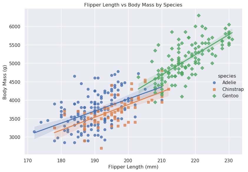
Figure2: Imagegeneratedbytheprovidedcode.
CaseStudy2:TipsDataset-InsightsforaRestaurant Manager
The tips datasetcouldrepresentrealdatafromarestaurantmanagerinterested inunderstandingcustomertippingbehavior.
1 sns.scatterplot(data=tips, 2 x="total_bill", y="tip", hue="day",
3 style="sex")
4 plt.title("TipAmountvsTotalBill")
5 plt.xlabel("TotalBill($)")
6 plt.ylabel("Tip($)")
7 plt.legend(title="Day/Sex")
8 plt.grid(True, linestyle="--", linewidth=0.5)
9 plt.tight_layout()
10 plt.show()
Observation:
• Higherbillstendtoreceivehighertips.
• Therelationshipvariesslightlyacrossdaysandcustomergender.
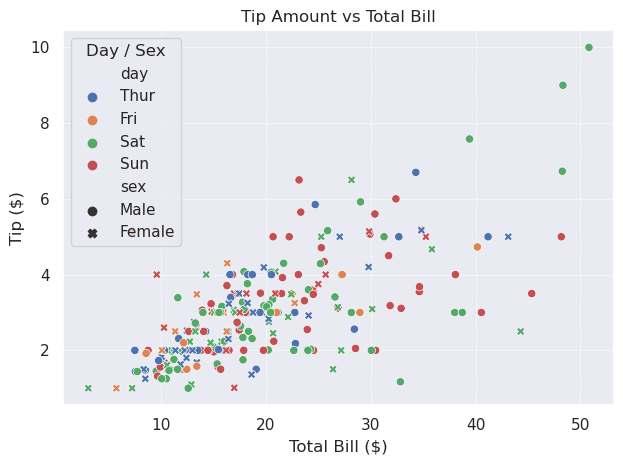
Figure3: Imagegeneratedbytheprovidedcode.
1 sns.catplot(data=tips, x="day", y="tip", hue="smoker", 2 kind="box", height=5, aspect=1.5)
3 plt.title("TipsbyDayandSmokerStatus")
4 plt.tight_layout()
5 plt.show()
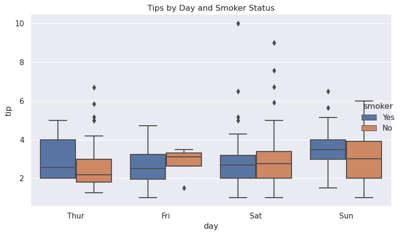
Figure4: Imagegeneratedbytheprovidedcode.
• Smokersandnon-smokersshowdi erenttippingpatternsdependingonthe day.
CaseStudy3:TimeTrendsintheFlightsDataset
Thisdatasetshowsthemonthlynumberofpassengersonanairlineoverseveral years.
1 flights_pivot = flights.pivot(index="month", 2 columns="year", 3 values="passengers")
5 sns.heatmap(flights_pivot, annot=True, fmt="d", cmap=" YlGnBu")
6 plt.title("MonthlyPassengerCounts(1949-1960)")
7 plt.xlabel("Year")
8 plt.ylabel("Month")
9 plt.tight_layout()
10 plt.show()
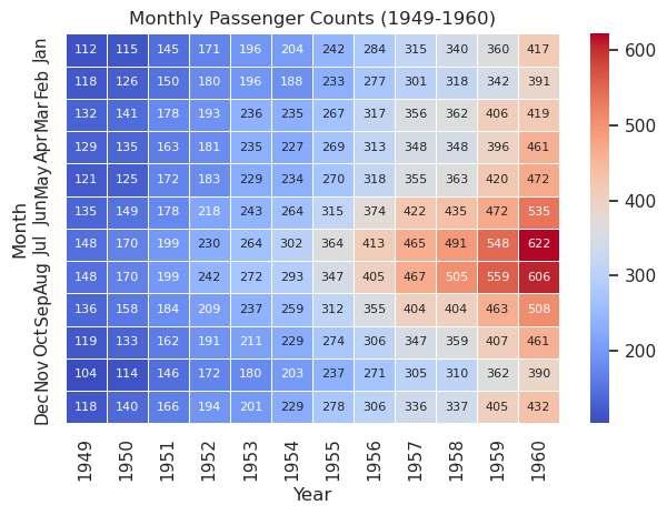
Figure5: Imagegeneratedbytheprovidedcode.
• Clearseasonalityisvisible.
• Passengercountsincreaseyearoveryear.
1 sns.clustermap(flights_pivot, cmap="coolwarm")
2 plt.show()
Figure6: Imagegeneratedbytheprovidedcode.
• Groupssimilarmonthsandyearsautomatically.
• Highlightspotentialpatternsandsimilarities.
Let’scombineseveralplotsintoasinglefigureasyouwouldforareportorpaper.
1 fig, axes = plt.subplots(2,2, figsize=(12,10))
sns.scatterplot(data=tips,
x="total_bill", y="tip", hue="day",
ax=axes[0,0]) 7 axes[0,0].set_title("TotalBillvsTip")
x="day", y="tip", hue="smoker",
ax=axes[0,1])
axes[0,1].set_title("TipsbyDayandSmoker")
#Regressionplot
sns.regplot(data=penguins,
x="flipper_length_mm", y="body_mass_g",
ax=axes[1,0]) 19 axes[1,0].set_title("FlipperLengthvsBodyMass")
sns.heatmap(flights_pivot,
annot=True,
fmt="d",
cmap="coolwarm",
linewidths=0.5,
linecolor="white",
annot_kws={"size":8},
ax = axes[1,1])
axes[1,1].set_title("FlightsHeatmap")
32 plt.tight_layout() 33 plt.show()
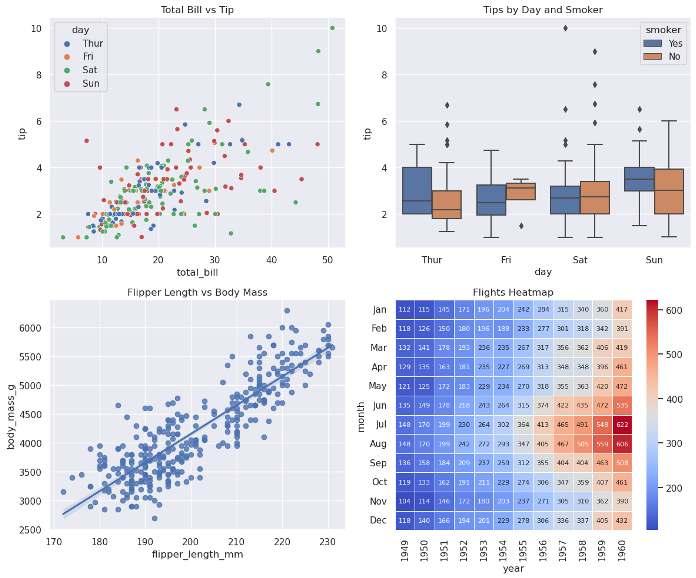
Figure7: Imagegeneratedbytheprovidedcode.
Notes
• Combiningdi erentSeabornplotsintoa singlefigure isapowerfulwayto communicatemultipleaspectsofyourdata.
• plt.subplots() + ax=axes[...] +Seabornplotsallowfortotalflexibility.
• Donotforgettoadjust titles, legends, fontsizes,and spacing whenpreparingfiguresforreportsorpublications.
• UseSeabornforitssimplebutpowerfulplottingfunctions.
• UseMatplotlibtocustomizedetailsandtoarrangeplotsasneeded.
• Combinebothlibrariestocreatecomplex,yetclearandinformativefigures.
Inthenextchapter,wewillsummarizeuseful TipsandTricks toimprove yourplotsevenmoreandavoidcommonpitfalls.
Inthischapter,wewillshareacollectionof practicaltips, commonpitfalls,and bestpractices thatwillhelpyou:
• Improvethequalityofyourplots.
• SavetimewhenworkingwithSeaborn.
• Avoidcommonmistakes.
• Prepareplotsfornotebooks,presentations,orpublications.
Theserecommendationsarebasedonreal-worldexperienceandareapplicable regardlessofyourlevelofexpertise.
Settingaglobalstyleavoidsinconsistentplotsacrossyournotebookorreport.
Tip2—Adjustfiguresizeearlywhenneeded
1 plt.figure(figsize=(8,6))
Thisavoidshavingtoresizeplotslaterorhavingplotstoosmallwhenexporting.
Tip3—Use hue, style,and size meaningfully
Theseargumentsarepowerfulbutcanmakeplotstoocrowdedifoverused. Alwaysaskyourself: Doesaddingcolororstyleimprovereadability?
Tip4—Use tight_layout() o en
1 plt.tight_layout()
Ithelpsautomaticallyfixspacingissues,especiallywhencombiningmultiple plots.
Seabornhandlestheplot,butMatplotlibisyourbestallyforannotations,arrows, textboxes,orpreciselayoutadjustments.
1 ax = sns.scatterplot(data=tips, x="total_bill", y="tip")
2 ax.annotate("Interestingpoint",
3 xy=(40,8),
4 xytext=(30,9),
5 arrowprops=dict(arrowstyle="->"))
1 plt.legend(loc="centerleft", bbox_to_anchor=(1,0.5))
Movinglegendsoutsidetheplotiso ennecessaryinpapersandslides.
1 fig, axes = plt.subplots(1,2, figsize=(12,5))
2 sns.boxplot(data=tips, x="day", y="tip", ax=axes[0])
3 sns.violinplot(data=tips, x="day", y="tip", ax=axes[1])
4 plt.tight_layout()
5 plt.show()
Itiso enclearertoshowtwocomplementaryplotssidebysidethantooverload one.
• Avoid overplotting:Don’tusetoomanyvariablesencodedvia hue, size, and style simultaneously.
• Alwayscheckiftheplothelpsansweryourquestion.
• Use colorcarefully:
– Avoidunnecessarycolors.
– Usecolorblind-friendlypalettes(e.g., "colorblind", "muted", " Set2").
• Customizelabels:change plt.title(), plt.xlabel(),and plt. ylabel() tomakeplotsself-explanatory.
Savingplotsproperly
1 plt.savefig("my_plot.png", 2 dpi=300, 3 bbox_inches="tight")
• Alwaysexportplotswithhighresolution(dpi=300)ifyouplantousethem inpapers.
• Use bbox_inches="tight" toremoveextrawhitespace.
Avoidexportingscreenshots:
Alwaysexportusing savefig() ratherthanscreenshotstopreservequalityand dimensions.
MistakeRecommendation
UsingdefaultlabelsAlwaysaddinformativetitlesandaxislabels
OverloadingwithvariablesUse hue, style,or size selectively IgnoringlegendsAlwaysadjustorcleanyourlegends
Forgettingtoadjustfigure size Use figsize or set_context() appropriately
Notcheckingcolorblind accessibility
Preferpaletteslike "colorblind" or "muted"
Seabornisdesignedtohelpyou:
• Produceinformative,clean,andbeautifulplotswithminimalcode.
• CombineeasilywithMatplotlibforadvancedcontrol.
• Focusonthestoryyouwanttotellthroughyourdata.
Visualizationisnotjustaboutmakingplots;it’saboutmaking insightsvisible.
Inthenext(andfinal)chapter,wewillprovidealistof Referencesand FurtherReading tohelpyoucontinuelearningandimprovingyourdata visualizationskills.
Thefollowingresourcesareo icialandmaintainedbytheSeabornandMatplotlib developers:
• SeabornO icialDocumentation https://seaborn.pydata.org/
• MatplotlibO icialDocumentation https://matplotlib.org/stable/index.html
• PandasO icialDocumentation https://pandas.pydata.org/docs/
• PythonDataScienceHandbook(JakeVanderPlas) https://jakevdp.github.io/PythonDataScienceHandbook/ RecommendedBooks
• DataVisualizationwithPythonandSeaborn
By:MarcGarcia
Afocusedbookonproducinge ectivevisualizationsusingSeaborn.
• PythonDataScienceHandbook
By:JakeVanderPlas
AcompleteguidetodatasciencewithPython,includingMatplotliband Seaborn.
• StorytellingwithData
By:ColeNussbaumerKnaflic
Highlyrecommendedtoimproveyourabilitytocommunicateinsights throughvisuals.
• FundamentalsofDataVisualization
By:ClausO.Wilke
Open-accessbookexplaininggoodpracticesindatavisualization.
https://clauswilke.com/dataviz/
• SeabornTutorials
https://seaborn.pydata.org/tutorial.html
• DataCampSeabornTutorial
https://www.datacamp.com/tutorial/seaborn-python-tutorial
• PracticalBusinessPythonBlog https://pbpython.com/
• TowardsDataScience(VisualizationCategory) https://towardsdatascience.com/tagged/data-visualization
• ColorBrewer2 (Colorblind-friendlypalettes) https://colorbrewer2.org/
• AdobeColorWheel (Forcreatingcustompalettes) https://color.adobe.com/
• SeabornColorPaletteReference
https://seaborn.pydata.org/tutorial/color_palettes.html
Tomasterdatavisualization:
1.Practicebyreproducingplotsfromarticles,papers,oronlinetutorials.
2. Analyzefiguresinscientificpublicationsandthinkaboutwhatworksand whatcouldbeimproved.
3.Experimentwithdi erentdatasetsandexploretheirrelationshipsvisually.
4.CombineSeabornwithMatplotlibwhenyouneedfullcontrol.
Visualizationisakeyskillforanydatascientist,analyst,orresearcher.Seaborn providesagentlelearningcurvewithpowerfultools,butalwaysremember: “Agoodplotisnotonlyinformativebutalsotellsastory.”
Keepexploring,experimenting,andrefiningyourvisualstorytellingskills! Thankyouforfollowingthisguide!