With the advent of integrated circuits and computers, the borders of formal engineering disciplines of electronic and mechanical engineering have become fluid and fuzzy. Most products in the marketplace are made up of interdependent electronic and mechanical components, and electronic/electrical engineers find themselves working in organizations that are involved in both mechanical and electronic or electrical activities; the same is true of many mechanical engineers. The field of mechatronics offers engineers the expertise needed to face these new challenges.
Mechatronics is defined as the synergistic combination of precision mechanical, electronic, control, and systems engineering, in the design of products and manufacturing processes. It relates to the design of systems, devices and products aimed at achieving an optimal balance between basic mechanical structure and its overall control. Mechatronics responds to industry's increasing demand for engineers who are able to work across the boundaries of narrow engineering disciplines to identify and use the proper combination of technologies for optimum solutions to today's increasingly challenging engineering problems. Understanding the synergy between disciplines makes students of engineering better communicators who are able to work in cross-disciplines and lead design teams which may consist of specialist engineers as well as generalists. Mechatronics covers a wide range of application areas including consumer product design, instrumentation, manufacturing methods, motion control systems, computer integration, process and device control, integration of functionality with embedded microprocessor control, and the design of machines, devices and systems possessing a degree of computer-based intelligence. Robotic manipulators, aircraft simulators, electronic traction control systems, adaptive suspensions, landing gears, air-conditioners under fuzzy logic control, automated diagnostic systems, micro electromechanical systems (MEMS), consumer products such as VCRs, driver-less vehicles are all examples of mechatronic systems. These systems depend on the integration of mechanical, control, and computer systems in order to meet demanding specifications, introduce 'intelligence' in mechanical hardware, add versatility and maintainability, and reduce cost
Competitiveness requires devices or processes that are increasingly reliable, versatile, accurate, feature-rich, and at the same time inexpensive. These objectives
can be achieved by introducing electronic controls and computer technology as integrated parts of machines and their components. Mechatronic design results in improvements both to existing products, such as in microcontrolled drilling machines, as well as to new products and systems. A key prerequisite in building successful mechatronic systems is the fundamental understanding of the three basic elements of mechanics, control, and computers, and the synergistic application of these in designing innovative products and processes. Although all three building blocks are very important, mechatronics focuses explicitly on their interaction, integration, and synergy that can lead to improved and cost-effective systems
Aims of this book
This book is designed to serve as a mechatronics course text The text serves as instructional material for undergraduates who are embarking on a mechatronic course, but contains chapters suitable for senior undergraduates and beginning postgraduates It is also valuable resource material for practicing electronic, electrical, mechanical, and electromechanical engineers.
Overview of contents
The elements covered include electronic circuits, computer and microcontroller interfacing to external devices, sensors, actuators, systems response, modeling, simulation, and electronic fabrication processes of product development of mechatronic systems Reliability, an important area missed out in most mechatronic textbooks, is included.
Detailed contents - A route map
The book covers the following topics Chapter 1 introduces mechatronics Chapter 2 provides the reader with a review of electrical components and circuit elements and analysis. Chapter 3 presents semiconductor electronic devices. Chapter 4 covers digital electronics Chapter 5 deals with analog electronics Chapter 6 deals with important aspects of microcontroller architecture and programming in order to interface with external devices. Chapter 7 covers data acquisition systems Chapter 8 presents various commonly used sensors in mechatronic systems. Chapters 9 and 10 present electrical and mechanical external devices, respectively, for actuating mechatronic systems Chapter 11 deals with interfacing microcontrollers with external devices for actuating mechatronic systems; this chapter is the handbook for practical applications of most integrated
Preface XV
circuits treated in this book. Chapter 12 deals with the modeling aspect of control theory, which is of considerable importance in mechatronic systems Chapter 13 presents the analysis aspect of control theory, while Chapter 14 deals with graphical techniques in control theory Chapter 15 presents robotic system fundamentals, which is an important area in mechatronics. Chapter 16 presents electronic fabrication process, which those working with mechatronic systems should be familiar with Chapter 17 deals with reliability in mechatronic systems; a topic often neglected in mechatronics textbooks. Finally Chapter 18 presents some case studies.
The design process and the design of machine elements are important aspects of mechatronics. While a separate chapter is not devoted to these important areas, which are important in designing mechatronic systems, the appendices present substantial information on design principles and mechanical actuation systems design and analysis.
Additional features and supplements
Specific and practical information on mechatronic systems that the author has been involved in designing are given throughout the book, and a chapter has been devoted to hands-on practical guides to interfacing microcontrollers and external actuators, which is fundamental to a mechatronic system.
End-of chapter problems
All end-of-chapter problems have been tested as tutorials in the classroom at the University of the South Pacific A fully worked Solutions Manual is available for adopting instructors.
Online supplements to the text
For the student:
• Many of the exercises can be solved using MATLAB® and designs simulated using Simulink® (both from MathWorks Inc.). Copies of MATLAB® code used to solve the chapter exercises can be downloaded from the companion website http://books.elsevier.com/companions.
For the instructor:
• An Instructor's Solutions Manual is available for adopting tutors This provides complete worked solutions to the problems set at the end of each
chapter. To access this material please go to http://textbooks.elsevier.com and follow the instructions on screen.
Electronic versions of the figures presented are available for adopting lecturers to download for use as part of their lecture presentations. The material remains copyright of the author and may be used, with full reference to their source, only as part of lecture slides or handout notes They may not be used in any other way without the permission of the publisher.
CHAPTE R 1 Introduction to mechatronics
Chapter objectives
When you have finished this chapter you should be able to:
• trace the origin of mechatronics;
• understand the key elements of mechatronics systems;
• relate with everyday examples of mechatronics systems;
• appreciate how mechatronics integrates knowledge from different disciplines in order to realize engineering and consumer products that are useful in everyday life.
1.1 Historical perspective
Advances in microchip and computer technology have bridged the gap between traditional electronic, control and mechanical engineering. Mechatronics responds to industry's increasing demand for engineers who are able to work across the discipline boundaries of electronic, control and mechanical engineering to identify and use the proper combination of technologies for optimum solutions to today's increasingly challenging engineering problems All around us, we can find mechatronic products. Mechatronics covers a wide range of application areas including consumer product design, instrumentation, manufacturing methods, motion control systems, computer integration, process and device control, integration of functionality with embedded microprocessor control, and the design of machines, devices and systems possessing a degree of computer-based intelligence. Robotic manipulators, aircraft simulators, electronic traction control systems, adaptive suspensions, landing gears, air conditioners under fuzzy logic control, automated diagnostic systems, micro electromechanical systems (MEMS),
consumer products such as VCRs, and driver-less vehicles are all examples of mechatronic systems.
The genesis of mechatronics is the interdisciplinary area relating to mechanical engineering, electrical and electronic engineering, and computer science. This technology has produced many new products and provided powerful ways of improving the efficiency of the products we use in our daily life Currently, there is no doubt about the importance of mechatronics as an area in science and technology. However, it seems that mechatronics is not clearly understood; it appears that some people think that mechatronics is an aspect of science and technology which deals with a system that includes mechanisms, electronics, computers, sensors, actuators and so on. It seems that most people define mechatronics by merely considering what components are included in the system and/or how the mechanical functions are realized by computer software Such a definition gives the impression that it is just a collection of existing aspects of science and technology such as actuators, electronics, mechanisms, control engineering, computer technology, artificial intelligence, micro-machine and so on, and has no original content as a technology There are currently several mechatronics textbooks, most of which merely summarize the subject picked up from existing technologies. This structure also gives people the impression that mechatronics has no unique technology The definition that mechatronics is simply the combination of different technologies is no longer sufficient to explain mechatronics.
Mechatronics solves technological problems using interdisciplinary knowledge consisting of mechanical engineering, electronics, and computer technology To solve these problems, traditional engineers used knowledge provided only in one of these areas (for example, a mechanical engineer uses some mechanical engineering methodologies to solve the problem at hand) Later, due to the increase in the difficulty of the problems and the advent of more advanced products, researchers and engineers were required to find novel solutions for them in their research and development. This motivated them to search for different knowledge areas and technologies to develop a new product (for example, mechanical engineers tried to introduce electronics to solve mechanical problems). The development of the microprocessor also contributed to encouraging the motivation. Consequently, they could consider the solution to the problems with wider views and more efficient tools; this resulted in obtaining new products based on the integration of interdisciplinary technologies.
Mechatronics gained legitimacy in academic circles with the publication of the first refereed journal: IEEE/ASME Transactions on Mechatronics. In it, the authors worked tenaciously to define mechatronics Finally they coined the following:
The synergistic combination of precision mechanical engineering, electronic control and systems thinking in the design of products and manufacturing processes
Introduction to mechatronics
This definition supports the fact that mechatronics relates to the design of systems, devices and products aimed at achieving an optimal balance between basic mechanical structure and its overall control
1.2 Key elements of a mechatronic system
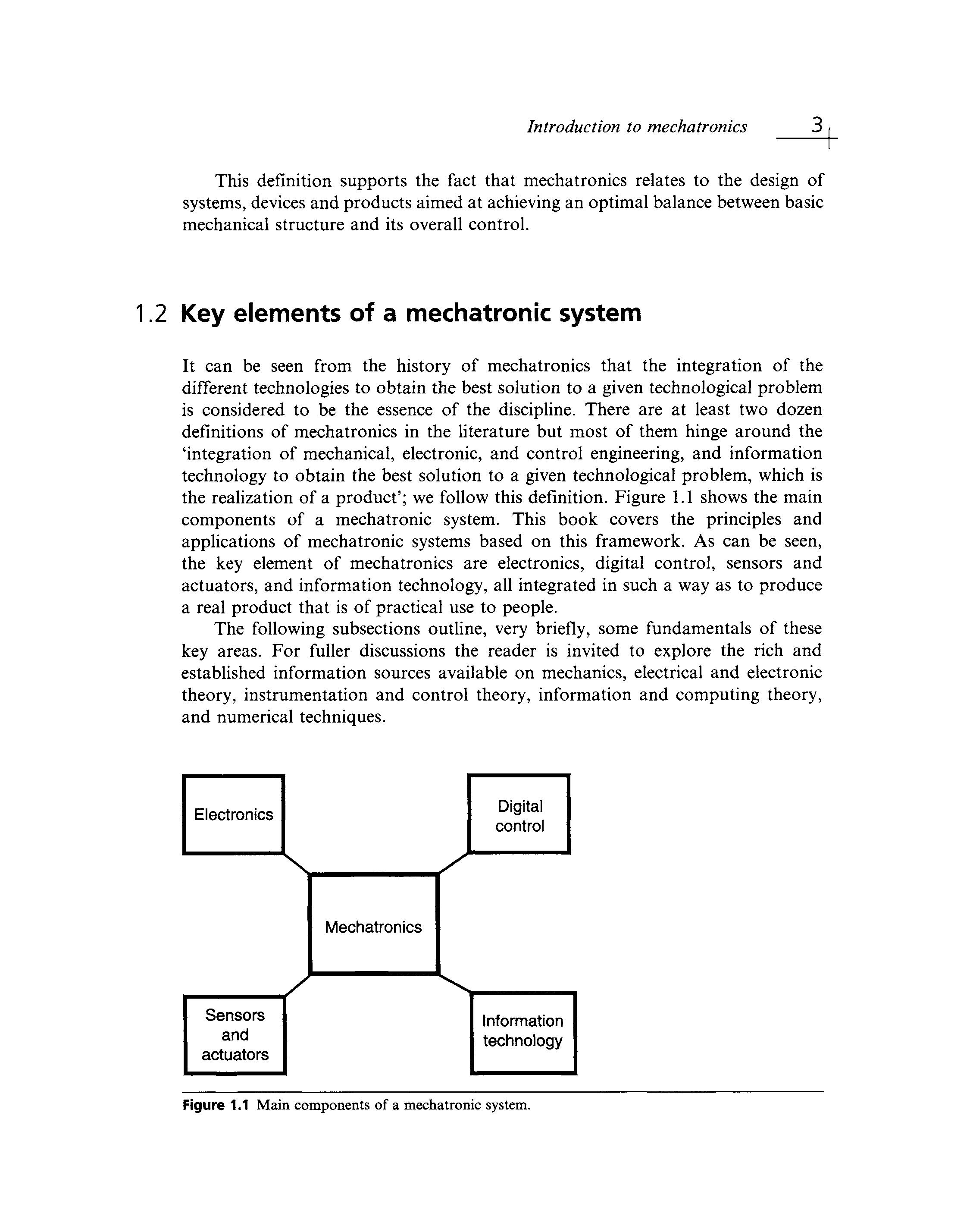
It can be seen from the history of mechatronics that the integration of the different technologies to obtain the best solution to a given technological problem is considered to be the essence of the discipline There are at least two dozen definitions of mechatronics in the literature but most of them hinge around the 'integration of mechanical, electronic, and control engineering, and information technology to obtain the best solution to a given technological problem, which is the realization of a product'; we follow this definition Figure 1.1 shows the main components of a mechatronic system. This book covers the principles and applications of mechatronic systems based on this framework. As can be seen, the key element of mechatronics are electronics, digital control, sensors and actuators, and information technology, all integrated in such a way as to produce a real product that is of practical use to people.
The following subsections outline, very briefly, some fundamentals of these key areas For fuller discussions the reader is invited to explore the rich and established information sources available on mechanics, electrical and electronic theory, instrumentation and control theory, information and computing theory, and numerical techniques.
Figure 1.1 Main components of a mechatronic system.
1.2.1 Electronics
1.2.1.1
Semiconductor devices
Semiconductor devices, such as diodes and transistors, have changed our lives since the 1950s. In practice, the two most commonly used semiconductors are germanium and silicon (the latter being most abundant and cost-effective) However, a semiconductor device is not made from simply one type of atom and impurities are added to the germanium or silicon base These impurities are highly purified tetravalent atoms (e.g. of boron, aluminum, gallium, or indium) and pentavalent atoms (e.g of phosphorus, arsenic, or antimony) that are called the doping materials. The effects of doping the semiconductor base material are 'free' (or unbonded) electrons, in the case of pentavalent atom doping, and 'holes' (or vacant bonds), in the case of tetravalent atoms.
An n-type semiconductor is one that has an excess number of electrons. A block of highly purified silicon has four electrons available for covalent bonding Arsenic, for, example, which is a similar element, has five electrons available for covalent bonding Therefore, when a minute amount of arsenic is mixed with a sample of silicon (one arsenic atom in every 1 million or so silicon atoms), the arsenic atom moves into a place normally occupied by a silicon atom and one electron is left out in the covalent bonding. When external energy (electrical, heat, or light) is applied to the semiconductor material, the excess electron is made to 'wander' through the material In practice, there would be several such extra negative electrons drifting through the semiconductor. Applying a potential energy source (battery) to the semiconductor material causes the negative terminal of the applied potential to repulse the free electrons and the positive terminal to attract the free electrons
If the purified semiconductor material is doped with a tetravalent atom, then the reverse takes place, in that now there is a deficit of electrons (termed 'holes'). The material is called a p-type semiconductor Applying an energy source results in a net flow of 'holes' that is in the opposite direction to the electron flow produced in n-type semiconductors
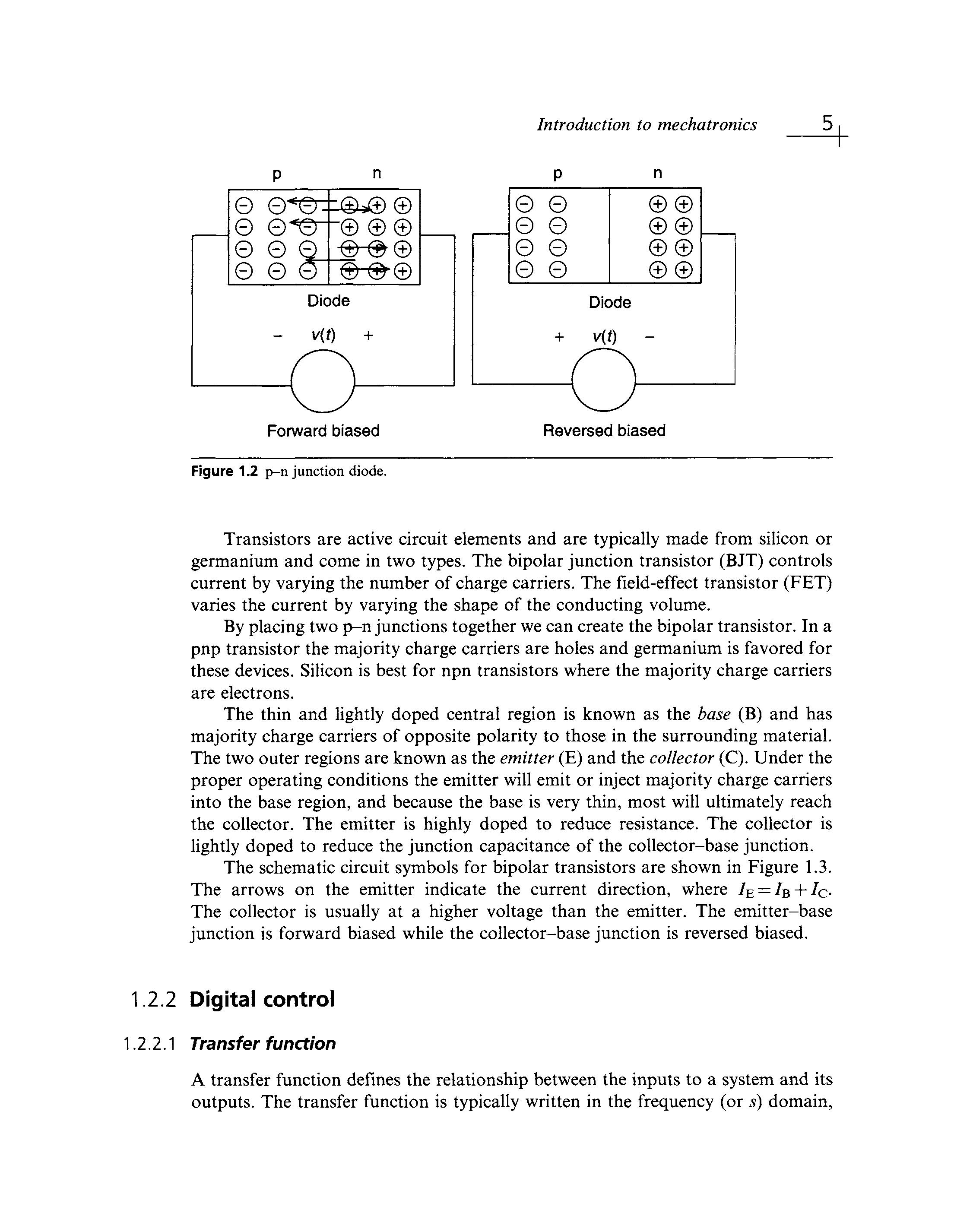
A semiconductor diode is formed by 'joining' a p-type and n-type semiconductor together as a p-n junction (Figure 1.2)
Initially both semiconductors are totally neutral. The concentration of positive and negative carriers is quite different on opposite sides of the junction and a thermal energy-powered diffusion of positive carriers into the n-type material and negative carriers into the p-type material occurs The n-type material acquires an excess of positive charge near the junction and the p-type material acquires an excess of negative charge. Eventually diffuse charges build up and an electric field is created which drives the minority charges and eventually equilibrium is reached A region develops at the junction called the depletion layer. This region is essentially 'un-doped' or just intrinsic silicon To complete the diode conductor, lead materials are placed at the ends of the p-n junction.
Figure 1.2 p-n junction diode.
Transistors are active circuit elements and are typically made from silicon or germanium and come in two types The bipolar junction transistor (BJT) controls current by varying the number of charge carriers. The field-effect transistor (FET) varies the current by varying the shape of the conducting volume.
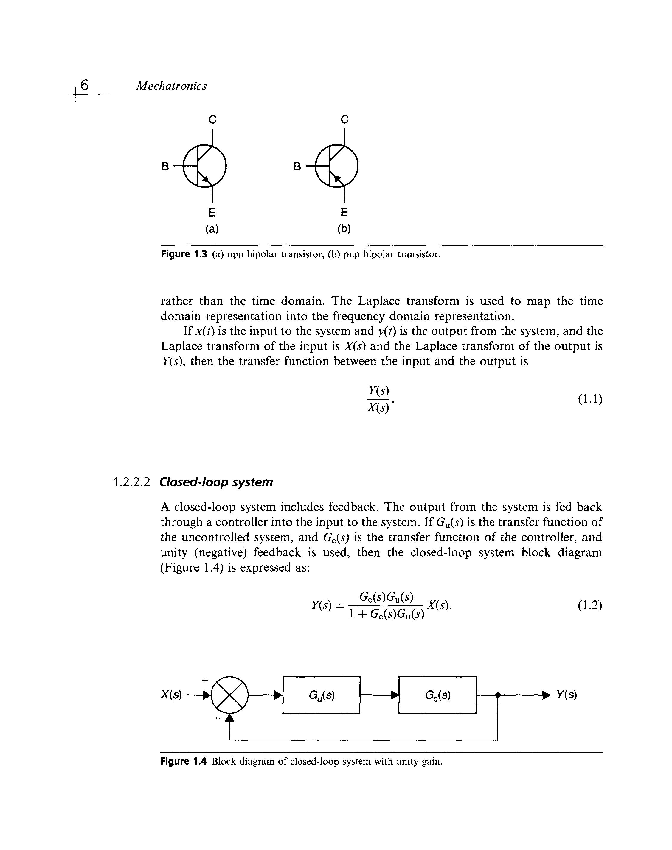
By placing two p-njunctions together we can create the bipolar transistor In a pnp transistor the majority charge carriers are holes and germanium is favored for these devices. Silicon is best for npn transistors where the majority charge carriers are electrons
The thin and lightly doped central region is known as the base (B) and has majority charge carriers of opposite polarity to those in the surrounding material The two outer regions are known as the emitter (E) and the collector (C). Under the proper operating conditions the emitter will emit or inject majority charge carriers into the base region, and because the base is very thin, most will ultimately reach the collector The emitter is highly doped to reduce resistance The collector is lightly doped to reduce the junction capacitance of the collector-base junction.
The schematic circuit symbols for bipolar transistors are shown in Figure 1.3 The arrows on the emitter indicate the current direction, where IE = IB + IC. The collector is usually at a higher voltage than the emitter. The emitter-base junction is forward biased while the collector-base junction is reversed biased
1.2.2 Digital control
1.2.2.1 Transfer function
A transfer function defines the relationship between the inputs to a system and its outputs The transfer function is typically written in the frequency (or s) domain,
rather than the time domain. The Laplace transform is used to map the time domain representation into the frequency domain representation If x(t) is the input to the system and y(i) is the output from the system, and the Laplace transform of the input is X(s) and the Laplace transform of the output is Y(s), then the transfer function between the input and the output is
1.2.2.2 Closed-loop system
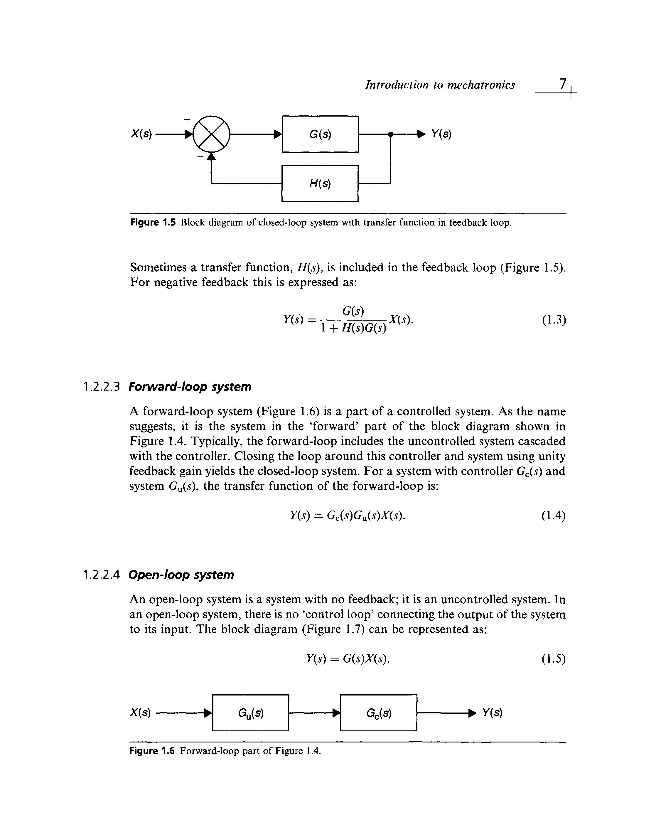
A closed-loop system includes feedback The output from the system is fed back through a controller into the input to the system. If Gu(s) is the transfer function of the uncontrolled system, and Gc(s) is the transfer function of the controller, and unity (negative) feedback is used, then the closed-loop system block diagram (Figure 1.4) is expressed as:
Figure 1.4 Block diagram of closed-loop system with unity gain.
Figure
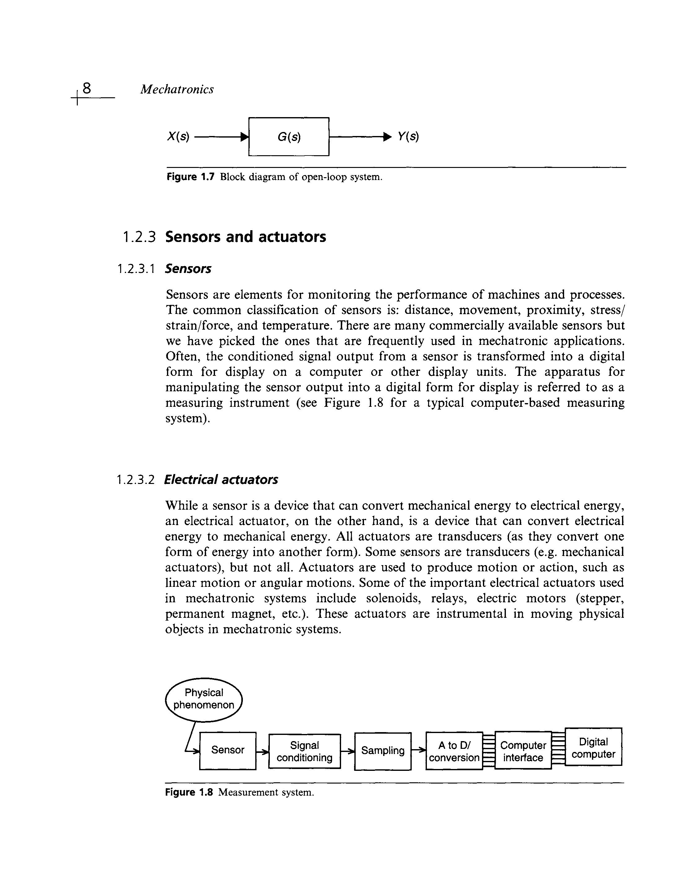
Figure 1.5 Block diagram of closed-loop system with transfer function in feedback loop
Sometimes a transfer function, H(s), is included in the feedback loop (Figure 1.5). For negative feedback this is expressed as:
= G(s) 1 + H(s)G(s)X(s).
1.2.2.3 Forward-loop system
A forward-loop system (Figure 1.6) is a part of a controlled system. As the name suggests, it is the system in the 'forward' part of the block diagram shown in Figure 1.4 Typically, the forward-loop includes the uncontrolled system cascaded with the controller. Closing the loop around this controller and system using unity feedback gain yields the closed-loop system. For a system with controller Gc(s) and system Ga(s), the transfer function of the forward-loop is:
= Gc(s)Gu(s)X(s).
1.2.2.4 Open-loop system
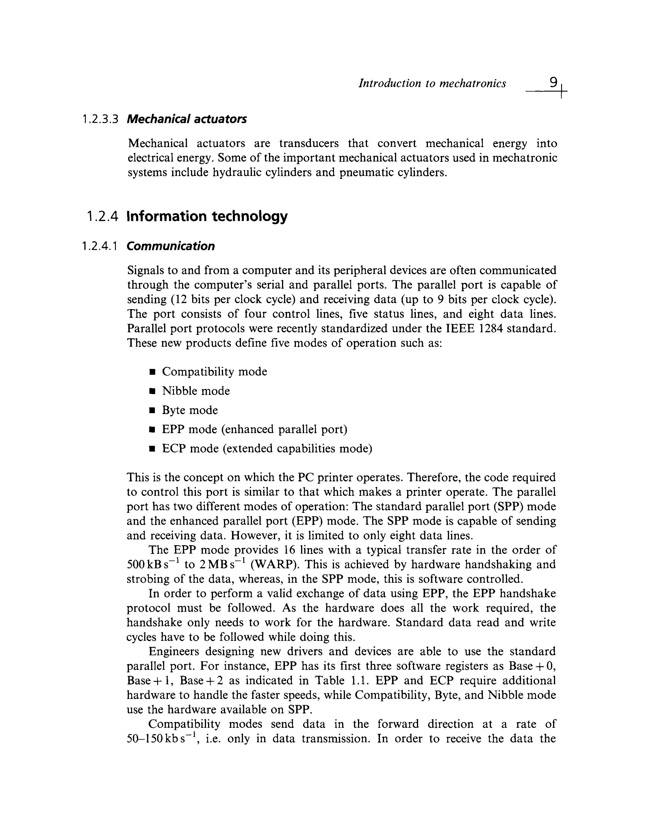
An open-loop system is a system with no feedback; it is an uncontrolled system. In an open-loop system, there is no 'control loop' connecting the output of the system to its input. The block diagram (Figure 1.7) can be represented as: Y(s) = G(s)X(s).
Figure 1.6 Forward-loop part of Figure 1.4.
1.2.3 Sensors and actuators
1.2.3.1 Sensors
Sensors are elements for monitoring the performance of machines and processes. The common classification of sensors is: distance, movement, proximity, stress/ strain/force, and temperature. There are many commercially available sensors but we have picked the ones that are frequently used in mechatronic applications. Often, the conditioned signal output from a sensor is transformed into a digital form for display on a computer or other display units. The apparatus for manipulating the sensor output into a digital form for display is referred to as a measuring instrument (see Figure 1.8 for a typical computer-based measuring system).
1.2.3.2 Electrical actuators
While a sensor is a device that can convert mechanical energy to electrical energy, an electrical actuator, on the other hand, is a device that can convert electrical energy to mechanical energy. All actuators are transducers (as they convert one form of energy into another form). Some sensors are transducers (e.g. mechanical actuators), but not all Actuators are used to produce motion or action, such as linear motion or angular motions. Some of the important electrical actuators used in mechatronic systems include solenoids, relays, electric motors (stepper, permanent magnet, etc.) These actuators are instrumental in moving physical objects in mechatronic systems.
Figure 1.7 Block diagram of open-loop system
Figure 1.8 Measurement system
1.2.3.3 Mechanical actuators
Mechanical actuators are transducers that convert mechanical energy into electrical energy Some of the important mechanical actuators used in mechatronic systems include hydraulic cylinders and pneumatic cylinders.
1.2.4 Information technology
1.2.4.1
Communication
Signals to and from a computer and its peripheral devices are often communicated through the computer's serial and parallel ports. The parallel port is capable of sending (12 bits per clock cycle) and receiving data (up to 9 bits per clock cycle). The port consists of four control lines, five status lines, and eight data lines. Parallel port protocols were recently standardized under the IEEE 1284 standard These new products define five modes of operation such as:
• Compatibility mode
• Nibble mode
• Byte mode
• EPP mode (enhanced parallel port)
• ECP mode (extended capabilities mode)
This is the concept on which the PC printer operates Therefore, the code required to control this port is similar to that which makes a printer operate. The parallel port has two different modes of operation: The standard parallel port (SPP) mode and the enhanced parallel port (EPP) mode. The SPP mode is capable of sending and receiving data. However, it is limited to only eight data lines.
The EPP mode provides 16 lines with a typical transfer rate in the order of 500kBs - 1 to 2MBs 1 (WARP). This is achieved by hardware handshaking and strobing of the data, whereas, in the SPP mode, this is software controlled.
In order to perform a valid exchange of data using EPP, the EPP handshake protocol must be followed. As the hardware does all the work required, the handshake only needs to work for the hardware. Standard data read and write cycles have to be followed while doing this.
Engineers designing new drivers and devices are able to use the standard parallel port For instance, EPP has its first three software registers as Base + 0, Base-Hi, Base+ 2 as indicated in Table 1.1. EPP and ECP require additional hardware to handle the faster speeds, while Compatibility, Byte, and Nibble mode use the hardware available on SPP.
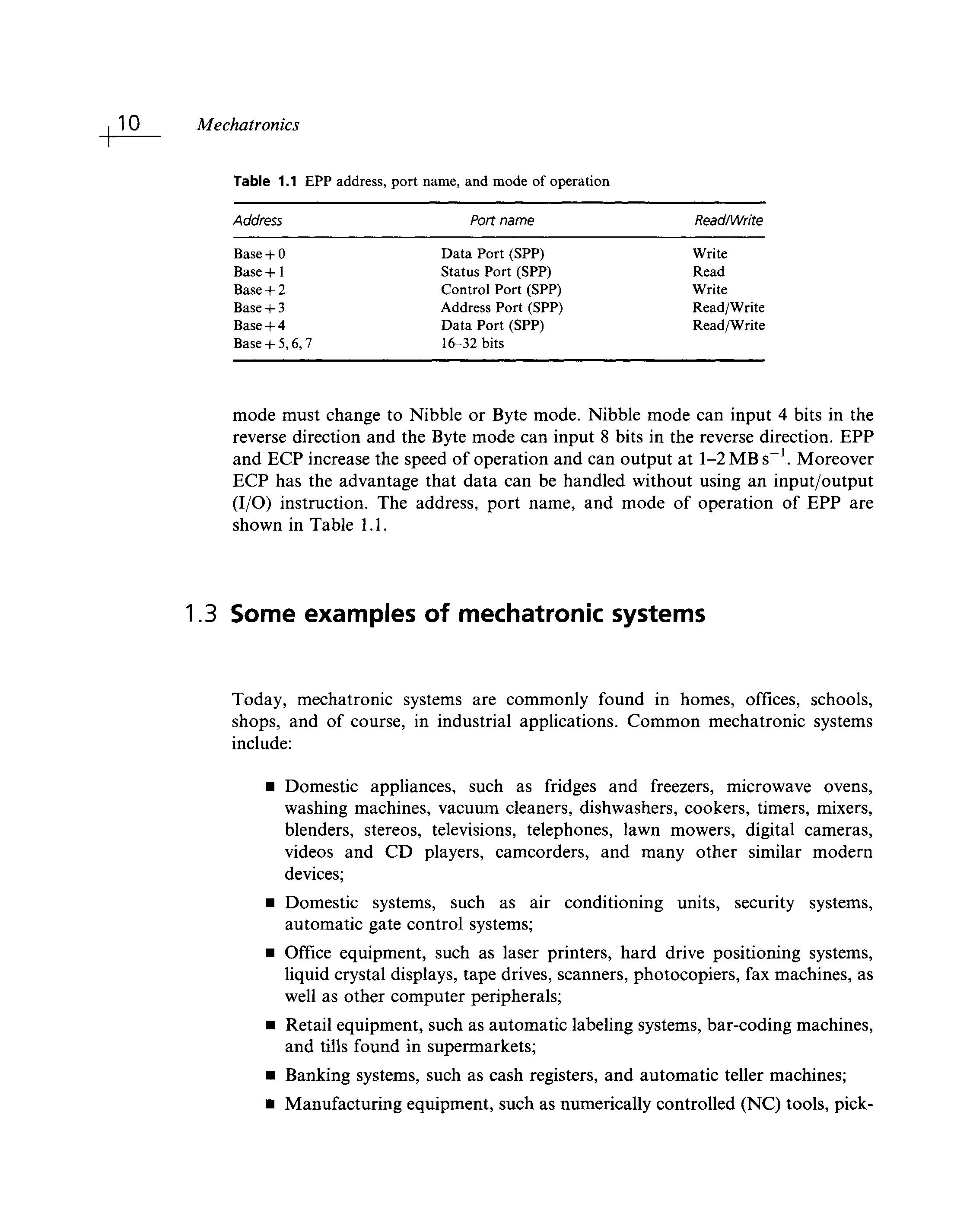
Compatibility modes send data in the forward direction at a rate of 50-150 kbs-1 , i.e. only in data transmission. In order to receive the data the
Table 1.1 EPP address, port name, and mode of operation
Address Port name
Base+ 0
Base+1
Base +2
Base + 3
Base + 4
Base + 5,6,7
Read/Write
Data Port (SPP)
Status Port (SPP)
Control Port (SPP)
Address Port (SPP)
Data Port (SPP) 16-32 bits Write
Read/Write
Read/Write
mode must change to Nibble or Byte mode. Nibble mode can input 4 bits in the reverse direction and the Byte mode can input 8 bits in the reverse direction. EPP and ECP increase the speed of operation and can output at 1-2 MB s_1 . Moreover ECP has the advantage that data can be handled without using an input/output (I/O) instruction The address, port name, and mode of operation of EPP are shown in Table 1.1
1.3 Some examples of mechatronic systems
Today, mechatronic systems are commonly found in homes, offices, schools, shops, and of course, in industrial applications. Common mechatronic systems include:
• Domestic appliances, such as fridges and freezers, microwave ovens, washing machines, vacuum cleaners, dishwashers, cookers, timers, mixers, blenders, stereos, televisions, telephones, lawn mowers, digital cameras, videos and CD players, camcorders, and many other similar modern devices;
• Domestic systems, such as air conditioning units, security systems, automatic gate control systems;
• Office equipment, such as laser printers, hard drive positioning systems, liquid crystal displays, tape drives, scanners, photocopiers, fax machines, as well as other computer peripherals;
• Retail equipment, such as automatic labeling systems, bar-coding machines, and tills found in supermarkets;
• Banking systems, such as cash registers, and automatic teller machines;
• Manufacturing equipment, such as numerically controlled (NC) tools, pick-
Introduction to mechatronics 1 1
and-place robots, welding robots, automated guided vehicles (AGVs), and other industrial robots;
• Aviation systems, such as cockpit controls and instrumentation, flight control actuators, landing gear systems, and other aircraft subsystems
Problems
Ql.l What do you understand by the term 'mechatronics'?
Q1.2 What are the key elements of mechatronics?
Q1.3 Is mechatronics the same as electronic engineering plus mechanical engineering?
Q1.4 Is mechatronics as established as electronic or mechanical engineering?
Q1.5 List some mechatronic systems that you see everyday
Further reading
[1] Alciatore, D and Histand, M (1995) Mechatronics at Colorado State University, Journal of Mechatronics, Mechatronics Education in the United States issue, Pergamon Press
[2] Jones, J.L and Flynn, A.M (1999) Mobile Robots: Inspiration to Implementation, 2nd Edition, Wesley, MA:A.K Peters Ltd
[3] Onwubolu, G.C et al. (2002) Development of a PC-based computer numerical control drilling machine, Journal of Engineering Manufacture, Short Communications in Manufacture and Design, 1509-15
[4] Shetty, D and Kolk, RA (1997) Mechatronics System Design, PWS Publishing Company
[5] Stiffler, A.K (1992) Design with Microprocessors for Mechanical Engineers, McGraw-Hill.
[6] Bolton, W (1995) Mechatronics - Electronic Control Systems in Mechanical Engineering, Longman.
[7] Bradley, D.A., Dawson, D., Burd, N.C. and Leader, A. J. (1993) MechatronicsElectronics in Products and Processes, Chapman & Hall.
[8] Fraser, C. and Milne, J. (1994) Integrated Electrical and Electronic Engineering for Mechanical Engineers, McGraw-Hill.
[9] Rzevski, G. (Ed). (1995) Perception, Cognition and Execution - Mechatronics: Designing Intelligent Machines, Vol. 1, Butterworth-Heinemann.
[10] Johnson, J. and Picton, P. (Eds) (1995) Concepts in Artificial IntelligenceMechatronics: Designing Intelligent Machines, Vol. 2.
[11] Miu, D. K. (1993) Mechatronics: Electromechanics and Contromechanics. SpringerVerlag.
[12] Auslander, D. M. and Kempf, C. J. (1996) Mechatronics: Mechanical System Interfacing, Prentice Hall.
[13] Bishop, R. H. (2002) The Mechatronics Handbook (Electrical Engineering Handbook Series), CRC Press.
[14] Braga, N.C. (2001) Robotics, Mechatronics and Artificial Intelligence: Experimental Circuit Blocks for Designers, Butterworth-Heinemann.
[15] Popovic, D. and Vlacic, L. (1999) Mechatronics in Engineering Design and Product Development, Marcel Dekker, Inc.
CHAPTE R 2
Electrical components and circuits
Chapter objectives
When you have finished this chapter you should be able to:
• understand the basic electrical components: resistor, capacitor, and inductor;
• deal with resistive elements using the node voltage method and the node voltage analysis method;
• deal with resistive elements using the mesh current method, principle of superposition, as well as Thevenin and Norton equivalent circuits;
• deal with sinusoidal sources and complex impedances.
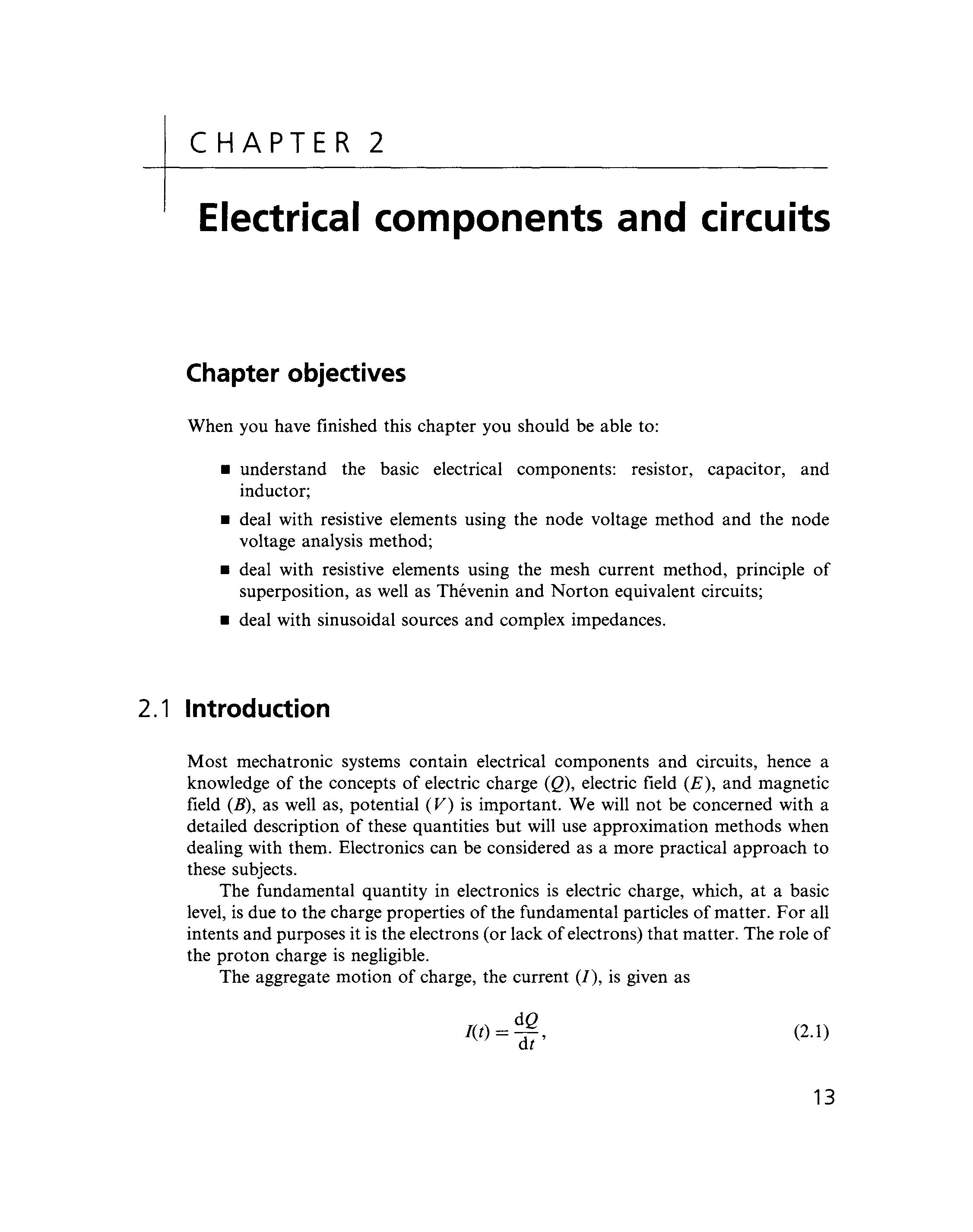
2.1 Introduction
Most mechatronic systems contain electrical components and circuits, hence a knowledge of the concepts of electric charge (Q), electric field (£), and magnetic field (B), as well as, potential (V) is important. We will not be concerned with a detailed description of these quantities but will use approximation methods when dealing with them Electronics can be considered as a more practical approach to these subjects.
The fundamental quantity in electronics is electric charge, which, at a basic level, is due to the charge properties of the fundamental particles of matter For all intents and purposes it is the electrons (or lack of electrons) that matter. The role of the proton charge is negligible.
The aggregate motion of charge, the current (/), is given as
where dQ is the amount of positive charge crossing a specified surface in a time dt. It is accepted that the charges in motion are actually negative electrons Thus the electrons move in the opposite direction to the current flow. The SI unit for current is the ampere (A) For most electronic circuits the ampere is a rather large unit so the milliampere (mA), or even the microampere (JLIA), unit is more common
Current flowing in a conductor is due to a potential difference between its ends. Electrons move from a point of less positive potential to more positive potential and the current flows in the opposite direction
It is often more convenient to consider the electrostatic potential (V) rather than the electric field (E) as the motivating influence for the flow of electric charge The generalized vector properties of E are usually not important. The change in potential d V across a distance dx in an electric field is
A positive charge will move from a higher to a lower potential. The potential is also referred to as the potential difference, or (incorrectly) as just voltage:
The SI unit of potential difference is the volt (V). Direct current (d.c.) circuit analysis deals with constant currents and voltages, while alternating current (a.c.) circuit analysis deals with time-varying voltage and current signals whose time average values are zero
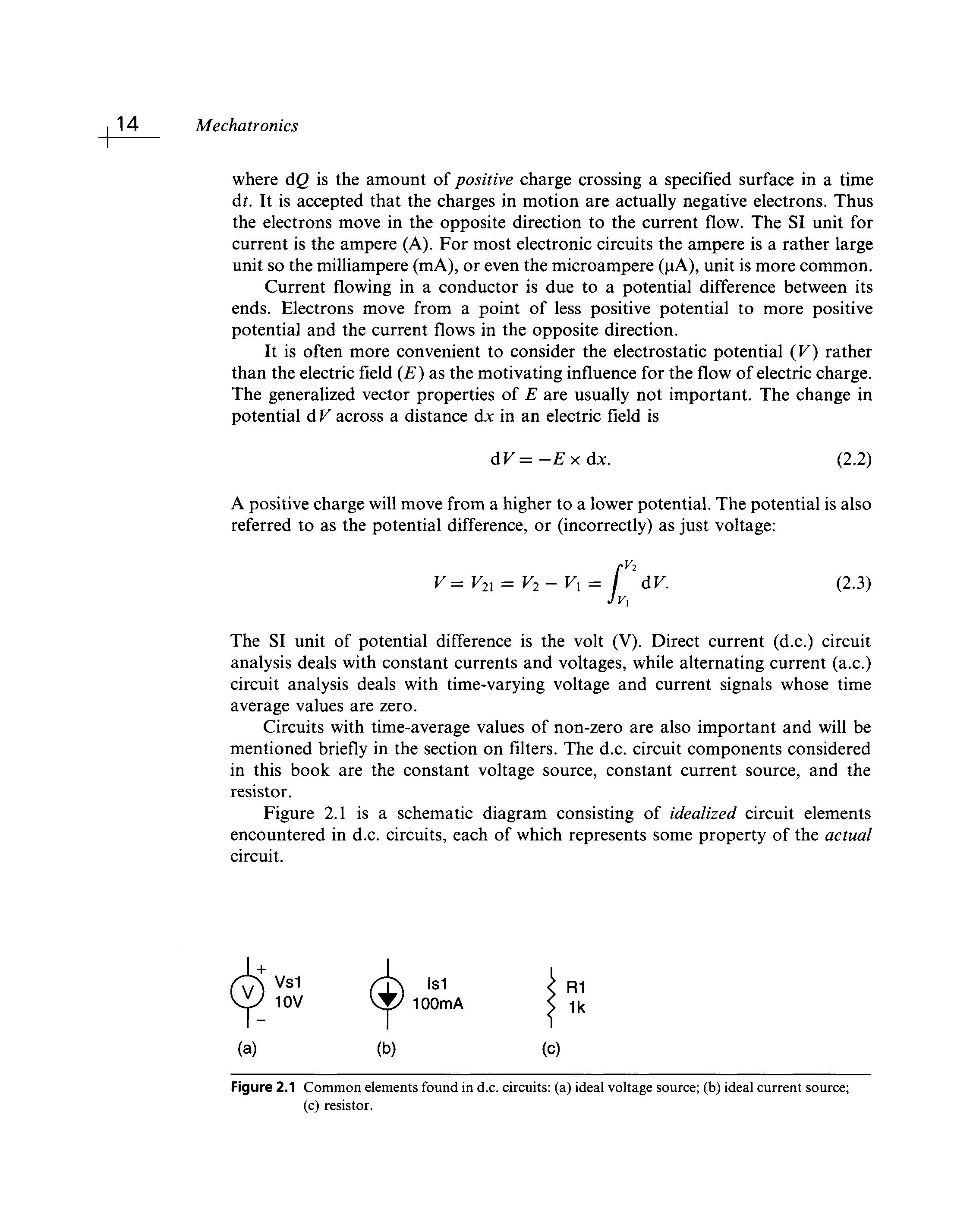
Circuits with time-average values of non-zero are also important and will be mentioned briefly in the section on filters. The d.c circuit components considered in this book are the constant voltage source, constant current source, and the resistor
Figure 2.1 is a schematic diagram consisting of idealized circuit elements encountered in d.c circuits, each of which represents some property of the actual circuit.
Figure 2.1 Common elements found in d.c circuits:(a) ideal voltage source; (b) ideal current source; (c) resistor.
2.1.1 External energy sources
Charge can flow in a material under the influence of an external electric field. Eventually the internal field due to the repositioned charge cancels the external electric field resulting in zero current flow. To maintain a potential drop (and flow of charge) requires an electromagnetic force (EMF), that is, an external energy source (battery, power supply, signal generator, etc.)
There are basically two types of EMFs that are of interest:
• the ideal voltage source, which is able to maintain a constant voltage regardless of the current it must put out (/ -» oo is possible);
• the ideal current source, which is able to maintain a constant current regardless of the voltage needed (V -> oo is possible).
Because a battery cannot produce an infinite amount of current, a suitable model for the behavior of a battery is an internal resistance in series with an ideal voltage source (zero resistance). Real-life EMFs can always be approximated with ideal EMFs and appropriate combinations of other circuit elements.
2.1.2 Ground
A voltage must always be measured relative to some reference point. We should always refer to a voltage (or potential difference) being 'across' something, and simply referring to voltage at a point assumes that the voltage point is stated with respect to ground. Similarly current flows through something, by convention, from a higher potential to a lower (do not refer to the current 'in' something) Under a strict definition, ground is the body of the Earth (it is sometimes referred to as earth). It is an infinite electrical sink. It can accept or supply any reasonable amount of charge without changing its electrical characteristics
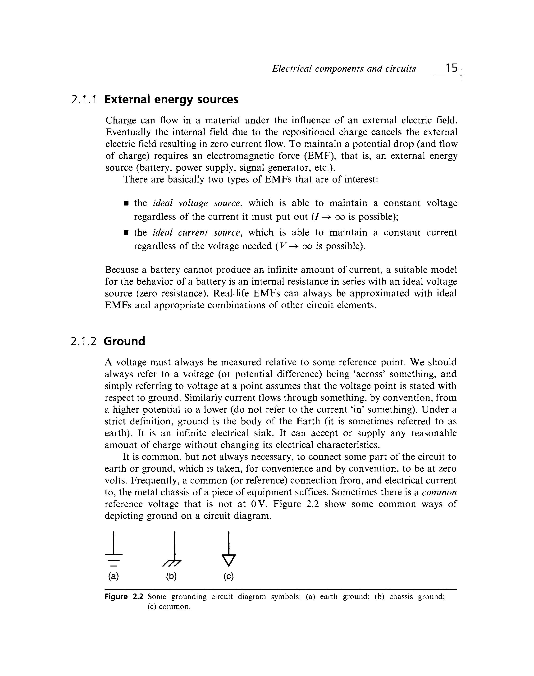
It is common, but not always necessary, to connect some part of the circuit to earth or ground, which is taken, for convenience and by convention, to be at zero volts Frequently, a common (or reference) connection from, and electrical current to, the metal chassis of a piece of equipment suffices. Sometimes there is a common reference voltage that is not at OV Figure 2.2 show some common ways of depicting ground on a circuit diagram.
When neither a ground nor any other voltage reference is shown explicitly on a schematic diagram, it is useful for purposes of discussion to adopt the convention that the bottom line on acircuit is at zero potential
Electrical components
The basic electrical components which are commonly used in mechatronic systems include resistors, capacitors, and inductors. The properties of these elements are now discussed
Resistance
Resistance is a function of the material and shape of the object, and has SI units of ohms (£2) It is more common to find units of kilohm (k£2) and megohm (M£2) The inverse of resistivity is conductivity.
Resistor tolerances can be as much as ±20 percent for general-purpose resistors to ±0.1 percent for ultra-precision resistors. Only wire-wound resistors are capable of ultra-precision accuracy
For most materials:
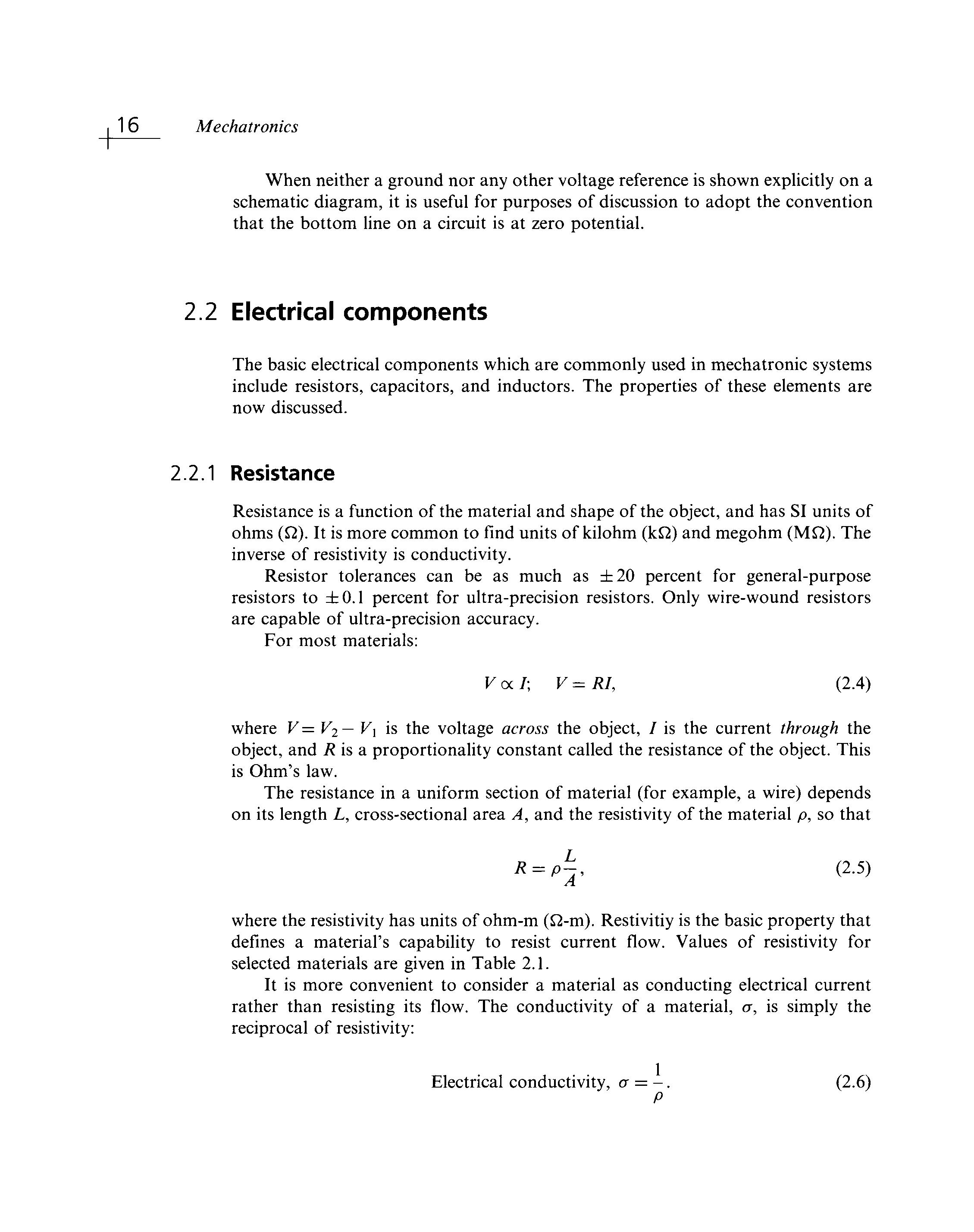
where V=V2—V\ is the voltage across the object, / is the current through the object, and R is a proportionality constant called the resistance of the object. This is Ohm's law
The resistance in a uniform section of material (for example, awire) depends on its length L, cross-sectional area A, and the resistivity of the material p, so that
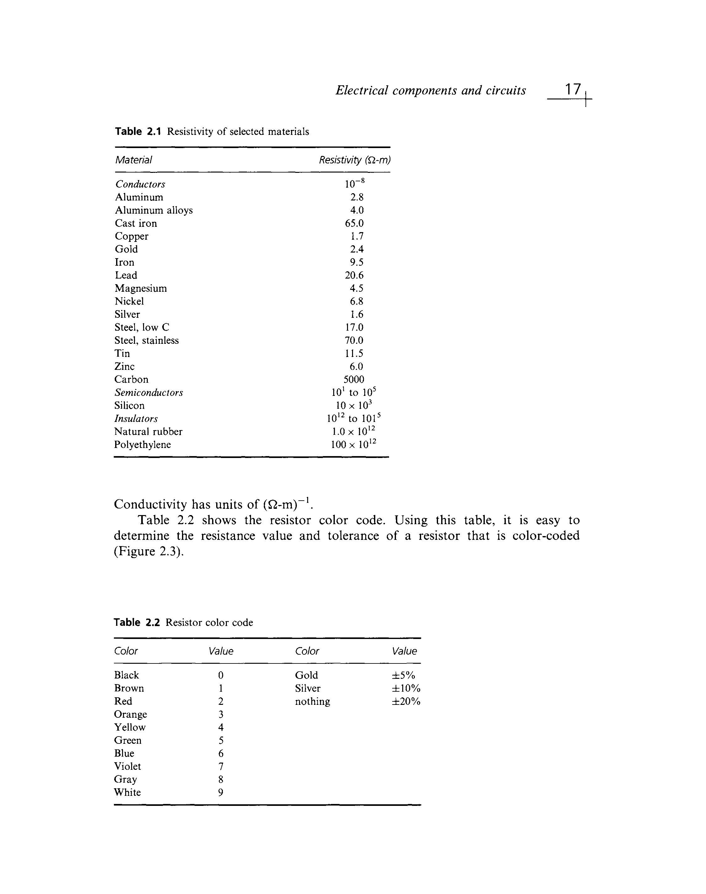
where the resistivity has units of ohm-m (Q-m). Restivitiy is the basic property that defines a material's capability to resist current flow Values of resistivity for selected materials are given in Table 2.1
It is more convenient to consider a material as conducting electrical current rather than resisting its flow. The conductivity of a material, a, is simply the reciprocal of resistivity:
components and circuits
Table 2.1 Resistivity of selected materials
Conductivity has units of (£2-m)~ .
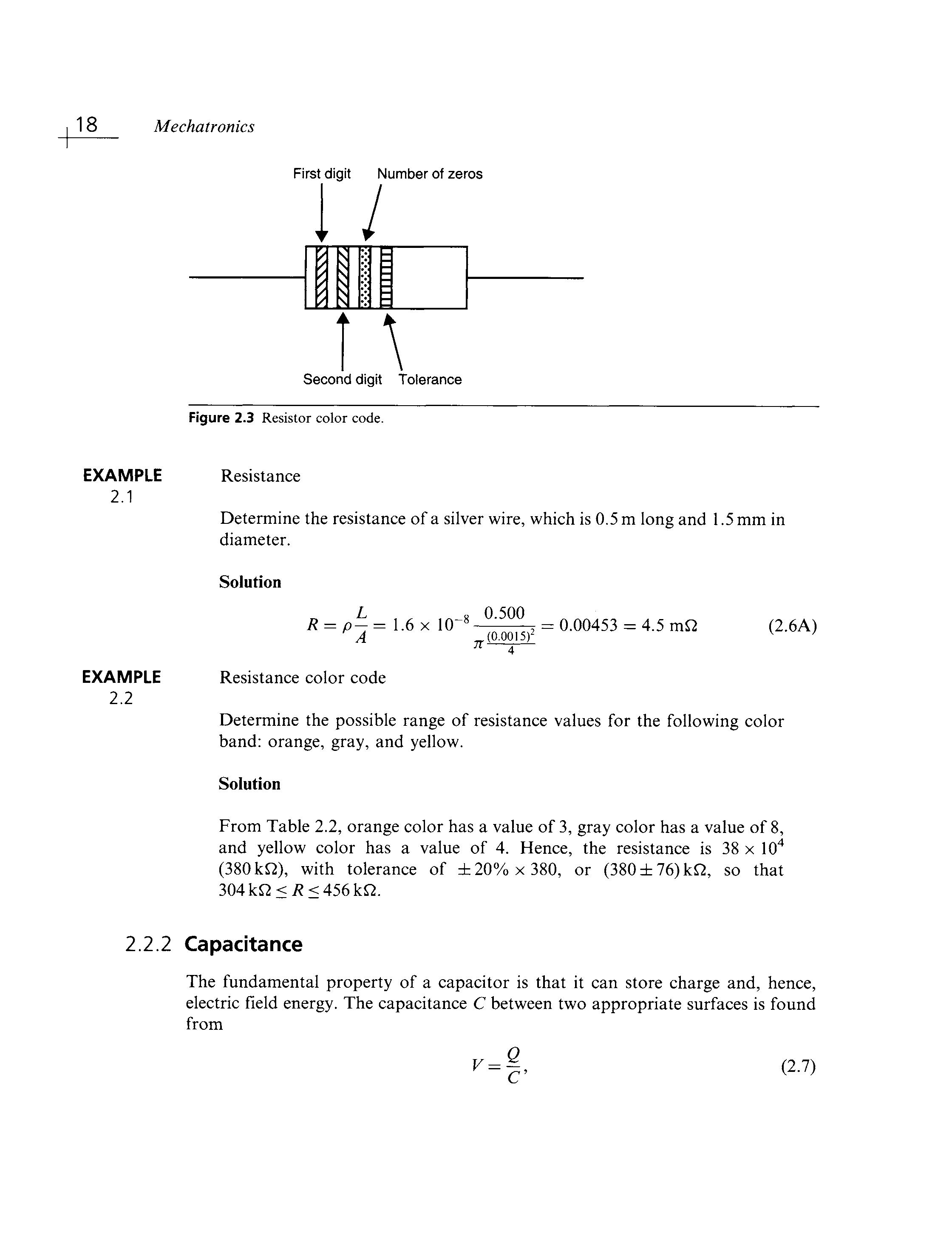
Table 2.2 shows the resistor color code. Using this table, it is easy to determine the resistance value and tolerance of a resistor that is color-coded (Figure 2.3).
Table 2.2 Resistor color code
Electrical components and circuits 19
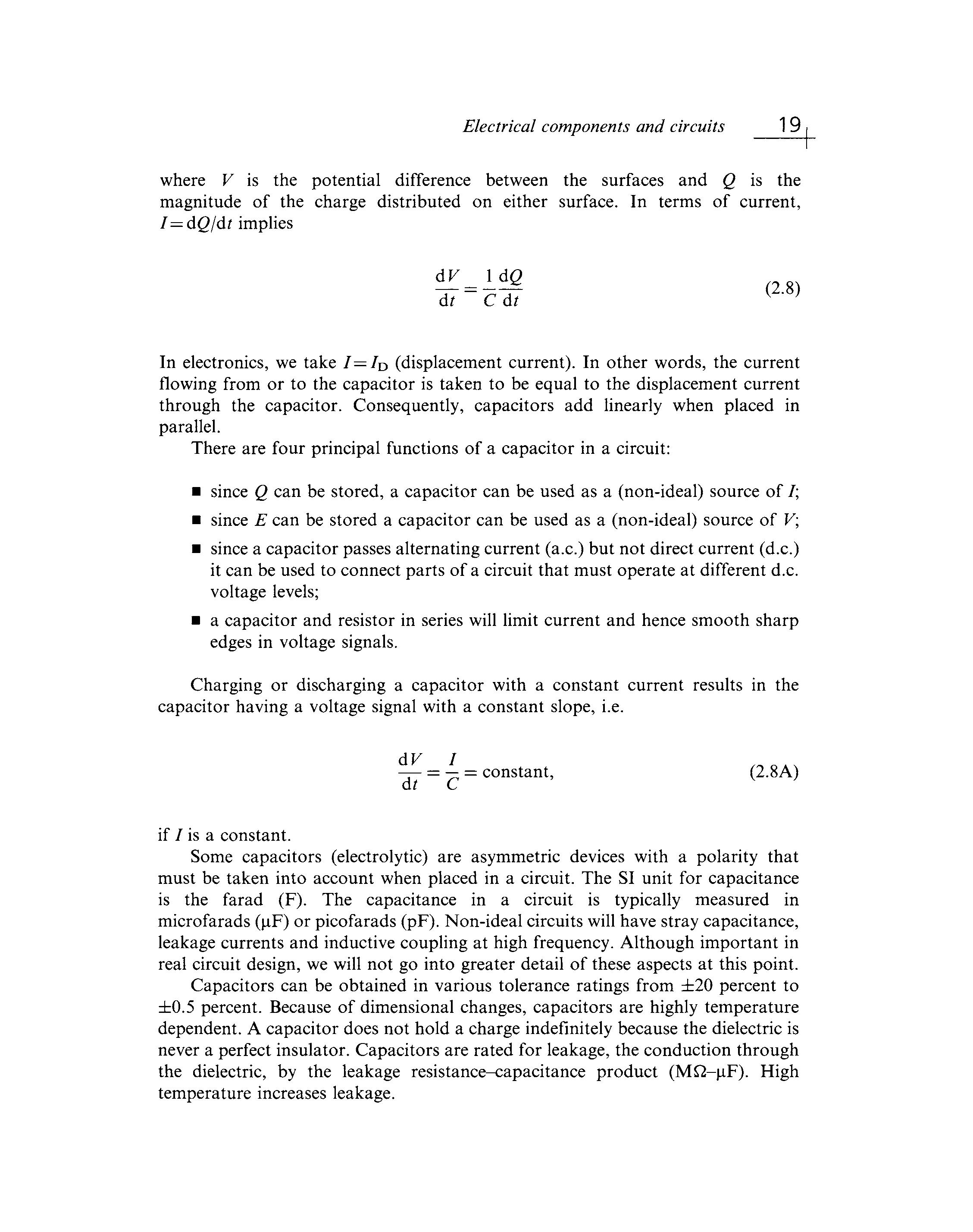
where V is the potential difference between the surfaces and Q is the magnitude of the charge distributed on either surface In terms of current, I=dQ/dt implies
In electronics, we take 7=/ D (displacement current) In other words, the current flowing from or to the capacitor is taken to be equal to the displacement current through the capacitor Consequently, capacitors add linearly when placed in parallel.
There are four principal functions of a capacitor in a circuit:
• since Q can be stored, a capacitor can be used as a (non-ideal) source of /;
• since E can be stored a capacitor can be used as a (non-ideal) source of V;
• since a capacitor passes alternating current (a.c.) but not direct current (d.c.) it can be used to connect parts of a circuit that must operate at different d.c voltage levels;
• a capacitor and resistor in series will limit current and hence smooth sharp edges in voltage signals.
Charging or discharging a capacitor with a constant current results in the capacitor having a voltage signal with a constant slope, i.e.
if / is a constant.
Some capacitors (electrolytic) are asymmetric devices with a polarity that must be taken into account when placed in a circuit The SI unit for capacitance is the farad (F). The capacitance in a circuit is typically measured in microfarads (jaF) or picofarads (pF) Non-ideal circuits will have stray capacitance, leakage currents and inductive coupling at high frequency Although important in real circuit design, we will not go into greater detail of these aspects at this point. Capacitors can be obtained in various tolerance ratings from ±20 percent to ±0.5 percent Because of dimensional changes, capacitors are highly temperature dependent. A capacitor does not hold a charge indefinitely because the dielectric is never a perfect insulator Capacitors are rated for leakage, the conduction through the dielectric, by the leakage resistance-capacitance product (M£2-|iF). High temperature increases leakage.
2.2.3 Inductance
Faraday's laws of electromagnetic induction applied to an inductor states that a changing current induces a back EMF that opposes the change. Putting this in another way,
A-VB=L^-, (2.9) at
where V is the voltage across the inductor and L is the inductance measured in henries (H). The more common units encountered in circuits are the microhenry (uH) and the millihenry (mH) The inductance will tend to smoothen sudden changes in current just as the capacitance smoothens sudden changes in voltage Of course, if the current is constant there will be no induced EMF. Hence, unlike the capacitor which behaves like an open-circuit in d.c circuits, an inductor behaves like a short-circuit in d.c. circuits.
Applications using inductors are less common than those using capacitors, but inductors are very common in high frequency circuits. Inductors are never pure (ideal) inductances because they always have some resistance in and some capacitance between the coil windings. We will skip the effect these have on a circuit at this stage
When choosing an inductor (occasionally called a choke) fora specific application, it is necessary to consider the value of the inductance, the d.c resistance of the coil, the current-carrying capacity of the coil windings, the breakdown voltage between the coil and the frame, and the frequency range in which the coil is designed to operate To obtain a very high inductance it is necessary to have a coil of many turns. Winding the coil on a closed-loop iron or ferrite core further increases the inductance To obtain as pure an inductance as possible, the d.c. resistance of the windings should be reduced toa minimum. Increasing the wire size, which, of course, increases the size of the choke, is the means of achieving this The size of the wire also determines the current-handling capacity of the choke since the work done in forcing a current through a resistance is converted to heat in the resistance. Magnetic losses in an iron core also account for some heating, and this heating restricts any choke to acertain safe operating current. The windings of the coil must be insulated from the frame as well as from each other Heavier insulation, which necessarily makes the choke more bulky, is used in applications where there will be a high voltage between the frame and the winding. The losses sustained in the iron core increases as the frequency increases. Large inductors, rated in henries, are used principally in power applications The frequency in these circuits is relatively low, generally 60Hz or low multiples thereof. In high-frequency circuits, such as those found in FM radios and television sets, very small inductors (of the order of microhenries) are often used
Now that we have briefly familiarized ourselves with these basic electrical elements, it is now necessary to consider the basic techniques for analyzing them.
2.3 Resistive circuits
The basic techniques for the analysis of resistive circuits are:
• node voltage and mesh current analysis;
• the principle of superposition;
• Thevenin and Norton equivalent circuits
The principle of superposition is a conceptual aid that can be very useful in visualizing the behavior of a circuit containing multiple sources. Thevenin and Norton equivalent circuits are the reductions of an arbitrary circuit to an equivalent, simpler circuit In this section it will be shown that it is generally possible to reduce all linear circuits to one of two equivalent forms, and that any linear circuit analysis problem can be reduced to a simple voltage or current divider problem.
2.3.1 Node voltage method
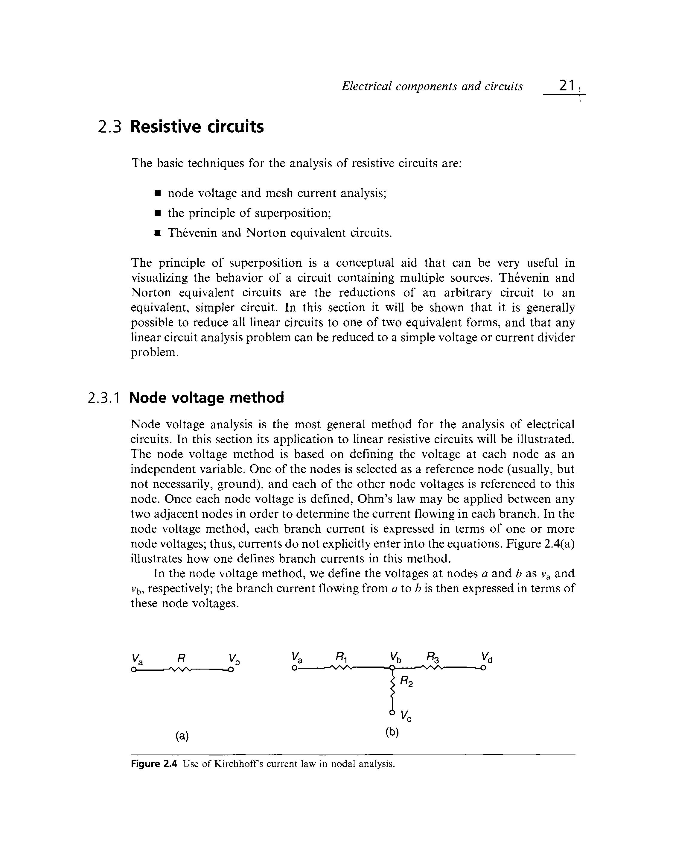
Node voltage analysis is the most general method for the analysis of electrical circuits In this section its application to linear resistive circuits will be illustrated The node voltage method is based on defining the voltage at each node as an independent variable. One of the nodes is selected as a reference node (usually, but not necessarily, ground), and each of the other node voltages is referenced to this node. Once each node voltage is defined, Ohm's law may be applied between any two adjacent nodes in order to determine the current flowing in each branch. In the node voltage method, each branch current is expressed in terms of one or more node voltages; thus, currents do not explicitly enter into the equations. Figure 2.4(a) illustrates how one defines branch currents in this method
In the node voltage method, we define the voltages at nodes a and b as va and vb, respectively; the branch current flowing from a to b is then expressed in terms of these node voltages
Figure 2.4 Use of Kirchhoff s current law in nodal analysis.
Once each branch current is defined in terms of the node voltages, Kirchhoff s current law (KCL) is applied at each node, so E/ = 0
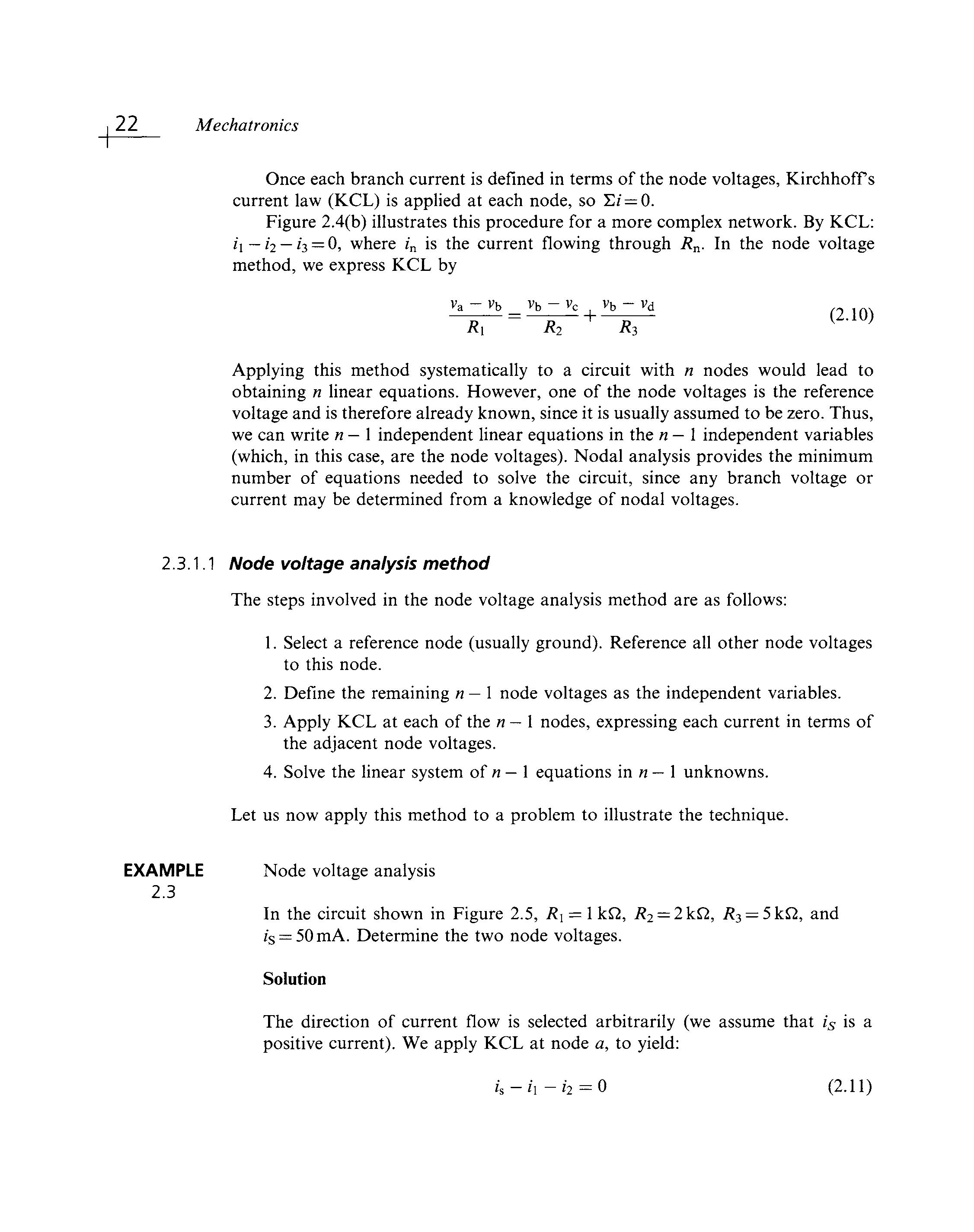
Figure 2.4(b) illustrates this procedure for a more complex network. By KCL: h — h — h = 0, where in is the current flowing through Rn In the node voltage method, we express KCL by
Applying this method systematically to a circuit with n nodes would lead to obtaining n linear equations. However, one of the node voltages is the reference voltage and is therefore already known, since it is usually assumed to be zero. Thus, we can write n — 1independent linear equations in the n — 1independent variables (which, in this case, are the node voltages). Nodal analysis provides the minimum number of equations needed to solve the circuit, since any branch voltage or current may be determined from a knowledge of nodal voltages
2.3.1.1 Node voltage analysis method
The steps involved in the node voltage analysis method are as follows:
1. Select a reference node (usually ground). Reference all other node voltages to this node
2. Define the remaining n — 1 node voltages as the independent variables.
3. Apply KCL at each of the n — 1 nodes, expressing each current in terms of the adjacent node voltages
4. Solve the linear system of n — 1 equations in n — 1 unknowns.
Let us now apply this method to a problem to illustrate the technique.
2.3
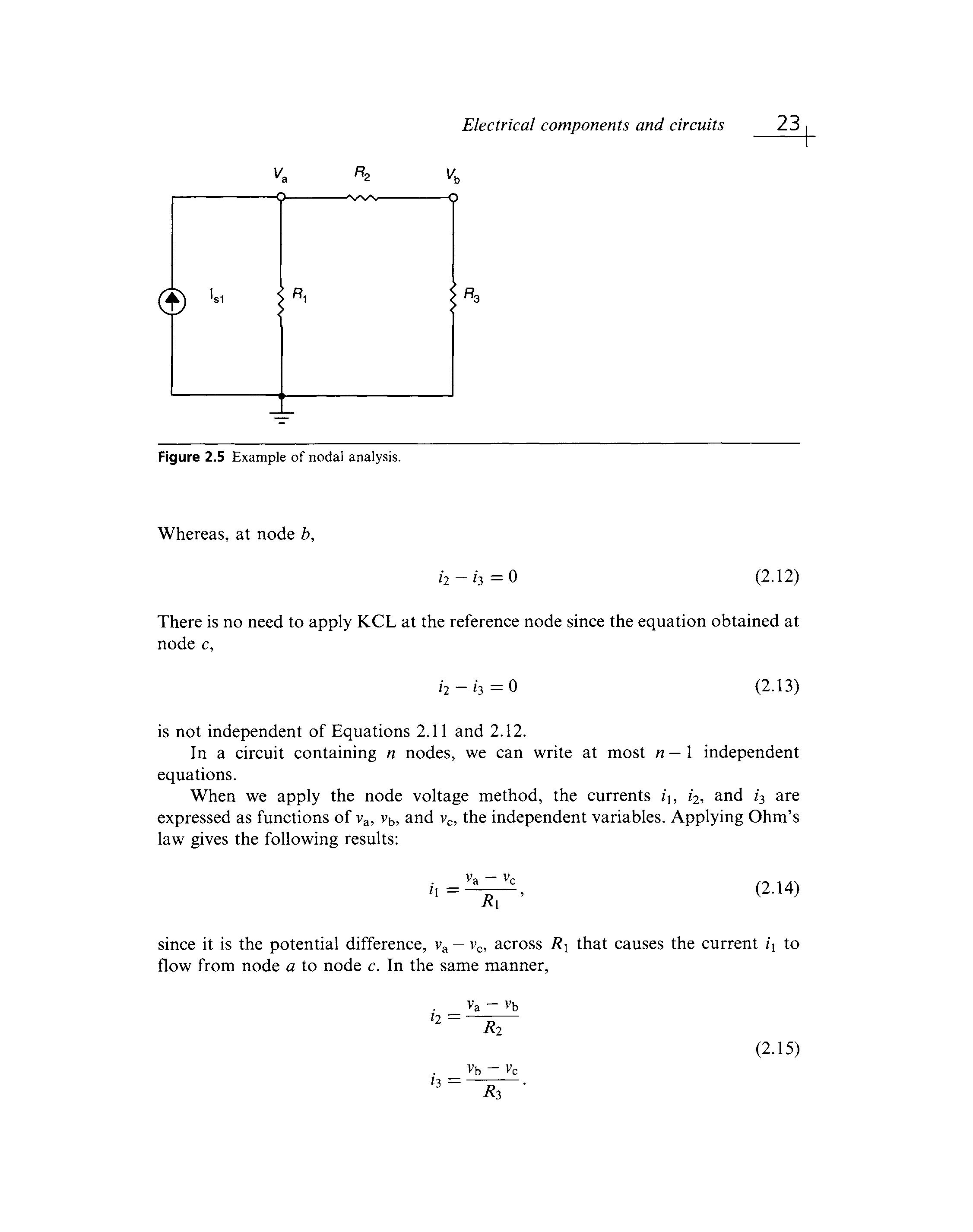
In the circuit shown in Figure 2.5, R\ = \ k£2, R2 = 2kQ, R3 = 5kQ, and /s = 50mA. Determine the two node voltages.
Solution
The direction of current flow is selected arbitrarily (we assume that is is a positive current) We apply KCL at node a, to yield:
Whereas, at node b,
h - h = 0 (2.12)
There is no need to apply KCL at the reference node since the equation obtained at node c,
h - h = 0 (2.13)
is not independent of Equations 2.11 and 2.12
In a circuit containing n nodes, we can write at most n — 1 independent equations
When we apply the node voltage method, the currents iu i2, and i3 are expressed as functions of va, vb, and vc, the independent variables Applying Ohm's law gives the following results:
since it is the potential difference, va — vc, across R\ that causes the current i\ to flow from node a to node c. In the same manner,
Figure 2.5 Example of nodal analysis.
Mechatronics
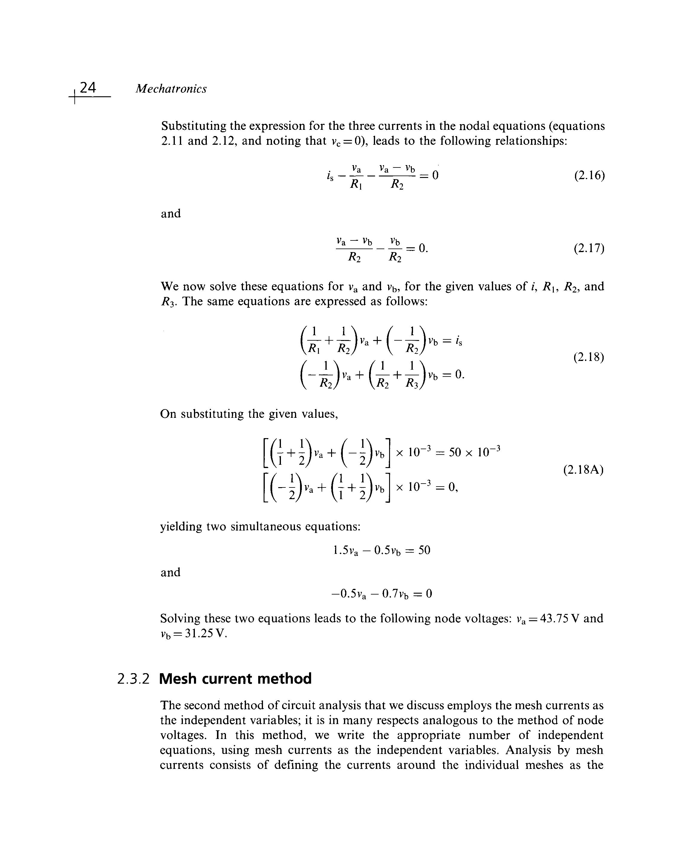
Substituting the expression for the three currents in the nodal equations (equations 2.11 and 2.12, and noting that vc = 0), leads to the following relationships: and
We now solve these equations for va and vb, for the given values of /, Ru R2, and R3 The same equations are expressed as follows:
On substituting the given values, (2.18) ,(l+^a+ (-0Vb]x 10"3 = 50 x 1(T3 x 1(T3 = 0, (2.18A)
yielding two simultaneous equations: 1.5va-0.5vb = 50 and -0.5va - 0.7vb = 0
Solving these two equations leads to the following node voltages: va = 43.75V and vb = 31.25 V.
2.3.2 Mesh current method
The second method of circuit analysis that we discuss employs the mesh currents as the independent variables; it is in many respects analogous to the method of node voltages. In this method, we write the appropriate number of independent equations, using mesh currents as the independent variables Analysis by mesh currents consists of defining the currents around the individual meshes as the
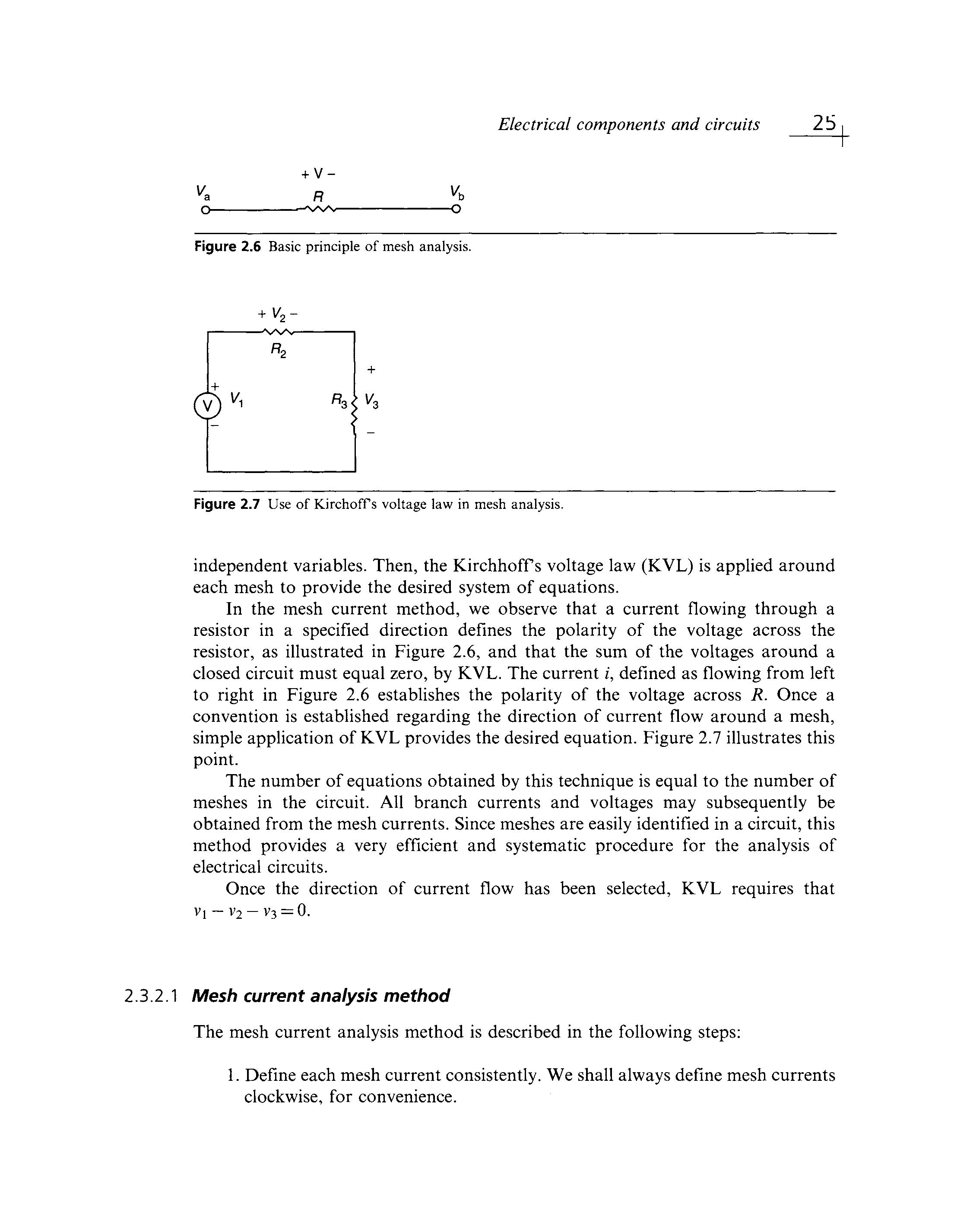
Figure 2.6 Basic principle of mesh analysis + VC
Figure 2.7 Use of Kirchoff s voltage law in mesh analysis
independent variables. Then, the Kirchhoff s voltage law (KVL) is applied around each mesh to provide the desired system of equations
In the mesh current method, we observe that a current flowing through a resistor in a specified direction defines the polarity of the voltage across the resistor, as illustrated in Figure 2.6, and that the sum of the voltages around a closed circuit must equal zero, by KVL The current i, defined as flowing from left to right in Figure 2.6 establishes the polarity of the voltage across 7?. Once a convention is established regarding the direction of current flow around a mesh, simple application of KVL provides the desired equation Figure 2.7 illustrates this point.
The number of equations obtained by this technique is equal to the number of meshes in the circuit All branch currents and voltages may subsequently be obtained from the mesh currents. Since meshes are easily identified in a circuit, this method provides a very efficient and systematic procedure for the analysis of electrical circuits
Once the direction of current flow has been selected, KVL requires that Vi — V2 — V3 = 0
2.3.2.1 Mesh current analysis method
The mesh current analysis method is described in the following steps:
1. Define each mesh current consistently. We shall always define mesh currents clockwise, for convenience
2 Apply KVL around each mesh, expressing each voltage in terms of one or more mesh currents.
3. Solve the resulting linear system of equations with mesh currents as the independent variables
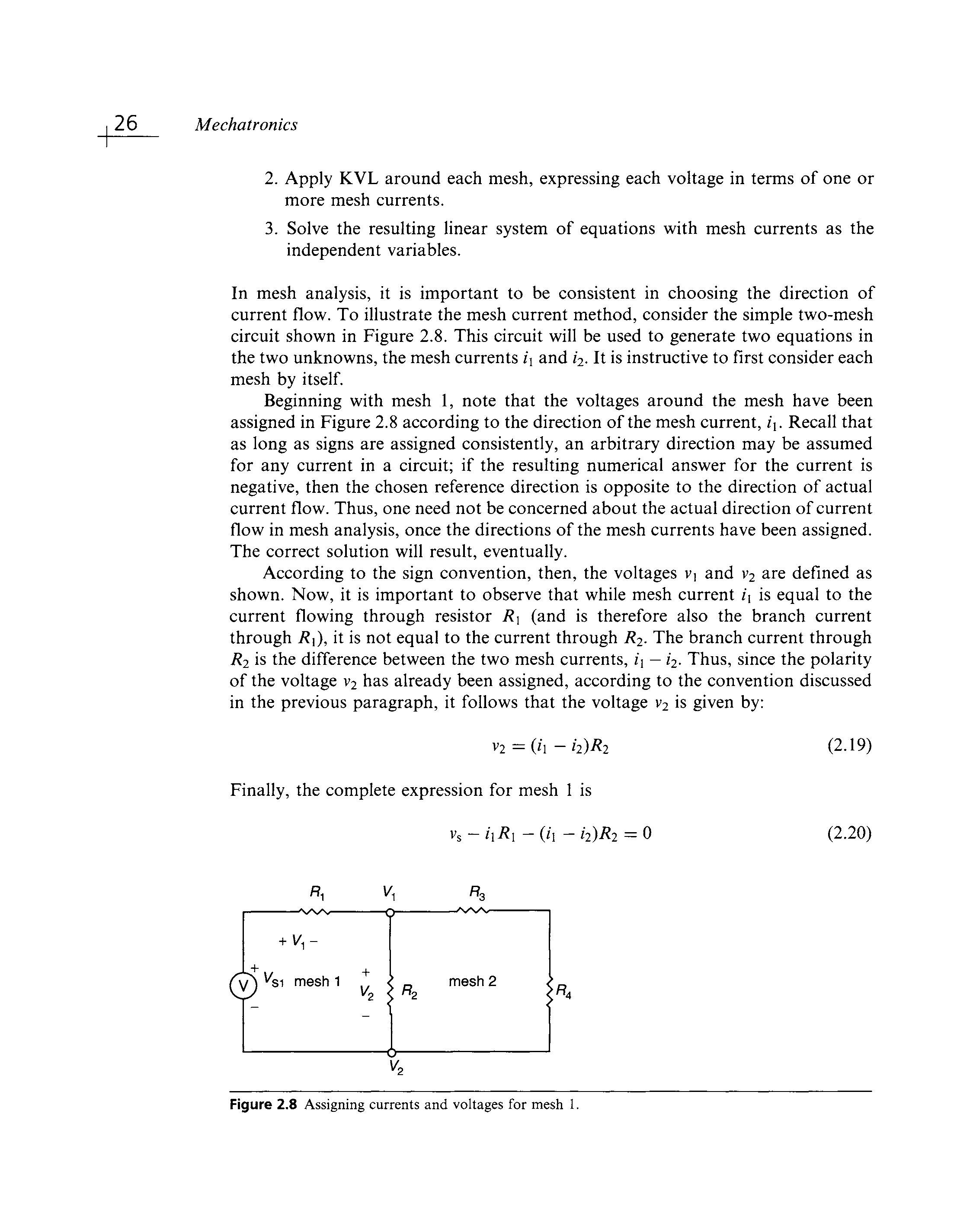
In mesh analysis, it is important to be consistent in choosing the direction of current flow. To illustrate the mesh current method, consider the simple two-mesh circuit shown in Figure 2.8. This circuit will be used to generate two equations in the two unknowns, the mesh currents i\ and i2 It is instructive to first consider each mesh by itself.
Beginning with mesh 1, note that the voltages around the mesh have been assigned in Figure 2.8 according to the direction of the mesh current, i\. Recall that as long as signs are assigned consistently, an arbitrary direction may be assumed for any current in a circuit; if the resulting numerical answer for the current is negative, then the chosen reference direction is opposite to the direction of actual current flow Thus, one need not be concerned about the actual direction of current flow in mesh analysis, once the directions of the mesh currents have been assigned. The correct solution will result, eventually According to the sign convention, then, the voltages vx and v2 are defined as shown. Now, it is important to observe that while mesh current ix is equal to the current flowing through resistor R\ (and is therefore also the branch current through R\), it is not equal to the current through R2 The branch current through R2 is the difference between the two mesh currents, ix — i2. Thus, since the polarity of the voltage v2 has already been assigned, according to the convention discussed in the previous paragraph, it follows that the voltage v2 is given by:
Finally, the complete expression for mesh 1 is
Figure 2.8 Assigning currents and voltages for mesh 1.
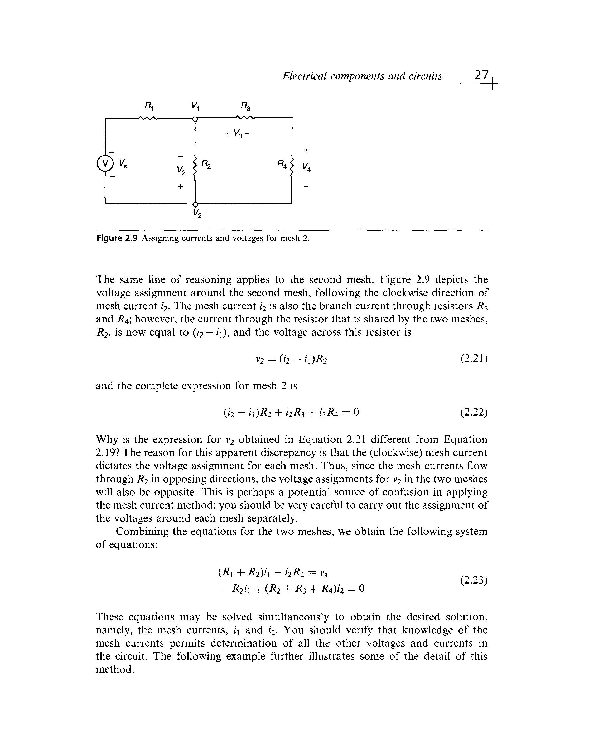
Figure 2.9 Assigning currents and voltages for mesh 2
The same line of reasoning applies to the second mesh. Figure 2.9 depicts the voltage assignment around the second mesh, following the clockwise direction of mesh current i2. The mesh current i2 is also the branch current through resistors R3 and R4; however, the current through the resistor that is shared by the two meshes, R2, is now equal to (i2 — i\), and the voltage across this resistor is
and the complete expression for mesh 2 is (2.22)
Why is the expression for v2 obtained in Equation 2.21 different from Equation 2.19? The reason for this apparent discrepancy is that the (clockwise) mesh current dictates the voltage assignment for each mesh. Thus, since the mesh currents flow through R2 in opposing directions, the voltage assignments for v2 in the two meshes will also be opposite. This is perhaps a potential source of confusion in applying the mesh current method; you should be very careful to carry out the assignment of the voltages around each mesh separately
Combining the equations for the two meshes, we obtain the following system of equations: (R{ + R2)h - i2R2 = vs - R2h + (R2 + ^3 + R4V2 = 0
(2.23)
These equations may be solved simultaneously to obtain the desired solution, namely, the mesh currents, ix and i2 You should verify that knowledge of the mesh currents permits determination of all the other voltages and currents in the circuit. The following example further illustrates some of the detail of this method.
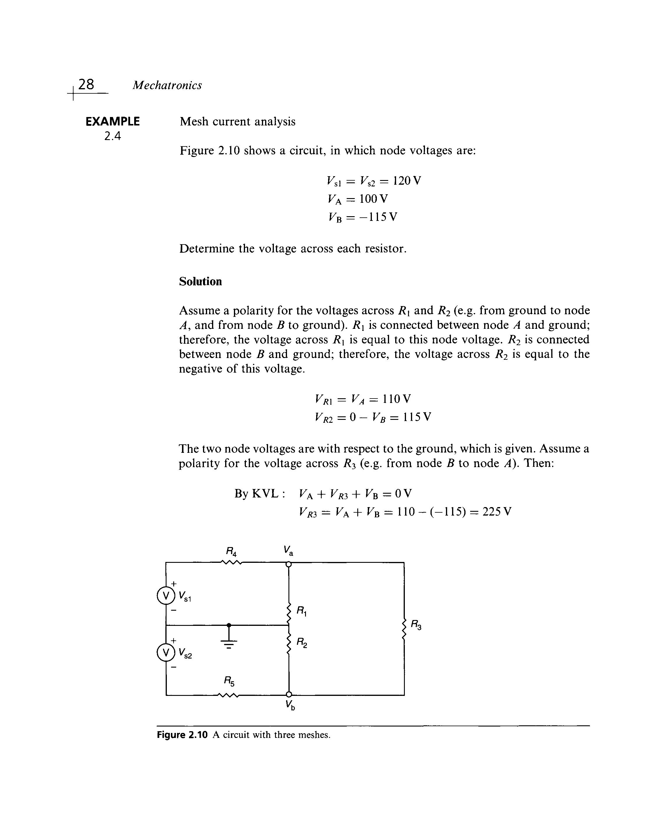
EXAMPLE 2.4
Mesh current analysis
Figure 2.10 shows a circuit, in which node voltages are:
Ksl = Ks2 = 120V
VA = 100V
KB =-115V
Determine the voltage across each resistor.
Solution
Assume a polarity for the voltages across R\ and R2 (e.g from ground to node A, and from node B to ground). R\ is connected between node A and ground; therefore, the voltage across R\ is equal to this node voltage. R2 is connected between node B and ground; therefore, the voltage across R2 is equal to the negative of this voltage.
VR2 = 0-VB=W5W
The two node voltages are with respect to the ground, which is given Assume a polarity for the voltage across RT, (e.g. from node B to node A). Then: ByKVL: KA + VR3 + KB = 0 V
R3 = KA + KB = 110 - (-115) = 225V
Figure 2.10 A circuit with three meshes
Assume the polarities for the voltages across R4 and R5 (e.g from node A to ground, and from ground to node B)\
ByKVL: Ksi + KJW + KA = OV
m = Ksi - VA = 120-110= 10 V
by KVL : - Vs2 - VB - VRS = 0V
2.3.3 The principle of superposition
This section briefly discusses a concept that is frequently called upon in the analysis of linear circuits Rather than a precise analysis technique, such as the mesh current and node voltage methods, the principle of superposition is a conceptual aid that can be very useful in visualizing the behavior of a circuit containing multiple sources. The principle of superposition applies to any linear system and for a linear circuit may be stated as follows:
In a linear circuit containing Nyfr sources, each branch voltage and current is the sum of Ni/r voltages and currents, each of which may be computed by setting all but one source equal to zero and solving the circuit containing that single source.
This principle can easily be applied to circuits containing multiple sources and is sometimes an effective solution technique More often, however, other methods result in a more efficient solution. We consider an example.
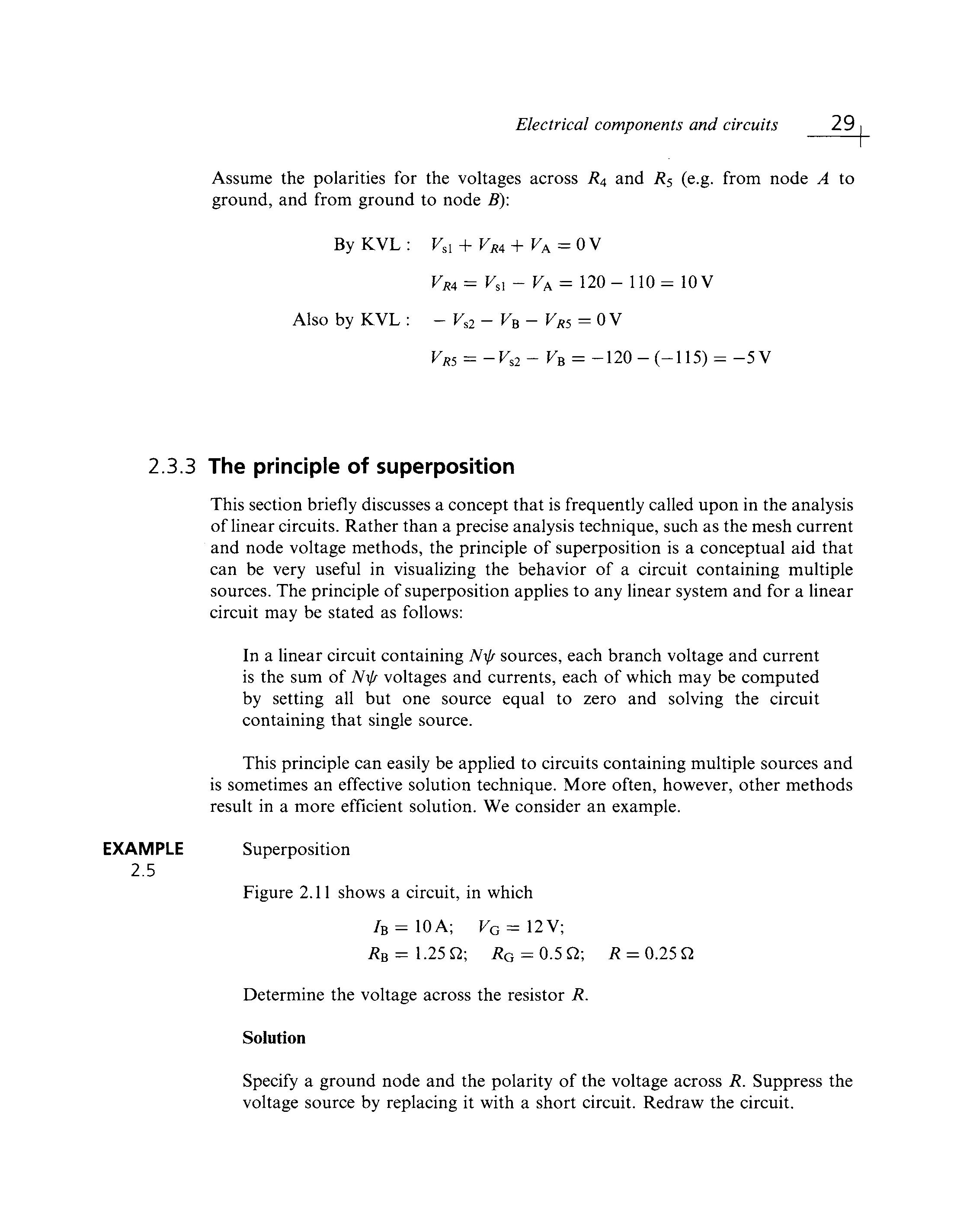
EXAMPLE Superposition
2.5
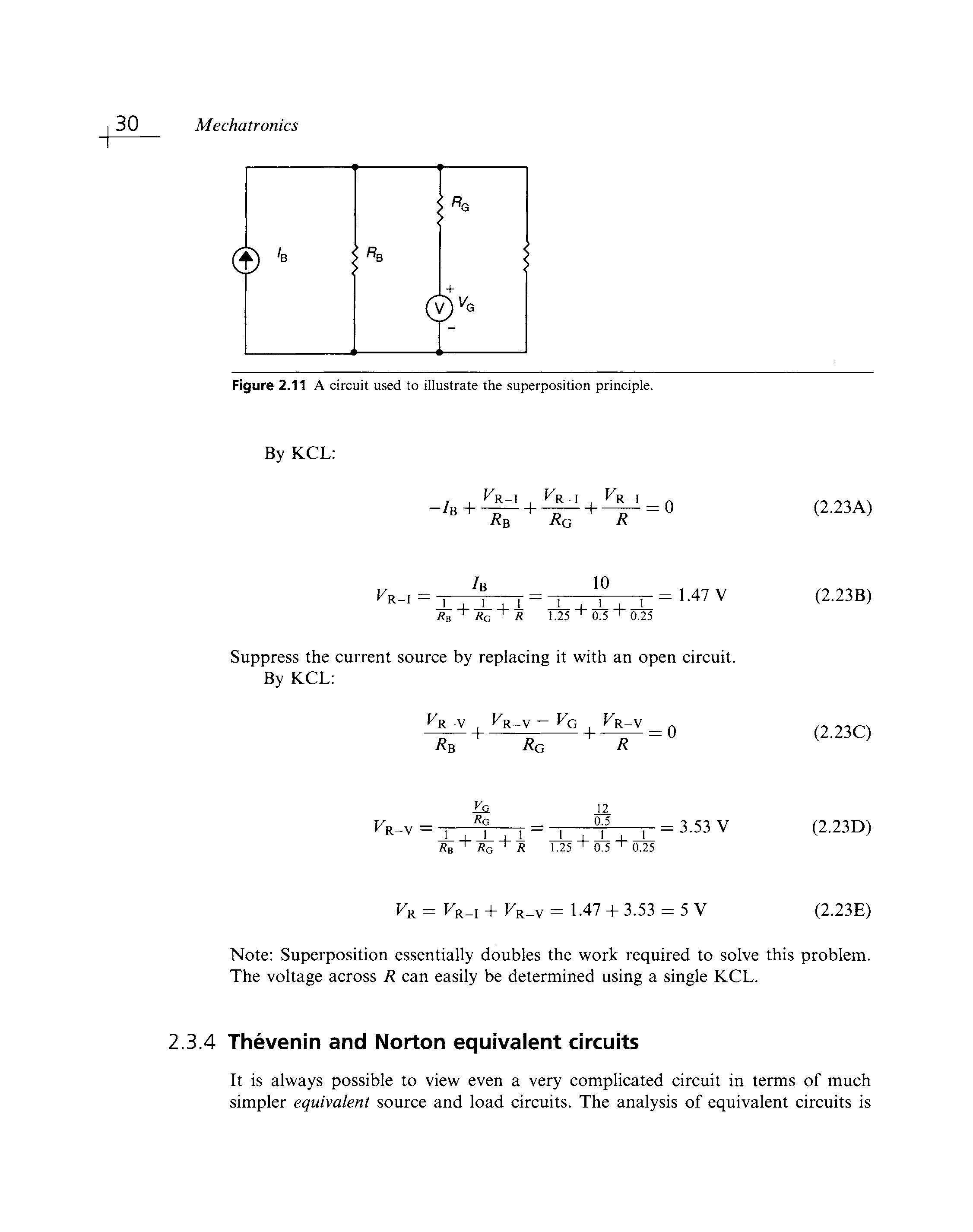
Figure 2.11 shows a circuit, in which /B = 10A; VG = 12V; RB = l.25Q; RG = 0.5Q\ R = 0.25Q
Determine the voltage across the resistor R.
Solution
Specify a ground node and the polarity of the voltage across R. Suppress the voltage source by replacing it with a short circuit Redraw the circuit
Figure 2.11 A circuit used to illustrate the superposition principle
By KCL:
Suppress the current source by replacing it with an open circuit By KCL:
Note: Superposition essentially doubles the work required to solve this problem The voltage across R can easily be determined using a single KCL.
2.3.4 Thevenin and Norton equivalent circuits
It is always possible to view even a very complicated circuit in terms of much simpler equivalent source and load circuits. The analysis of equivalent circuits is
more easily managed than the original complex circuit. In studying node voltage and mesh current analysis, you may have observed that there is a certain correspondence (called duality) between current sources and voltage sources, on the one hand, and parallel and series circuits, on the other. This duality appears again very clearly in the analysis of equivalent circuits: it will shortly be shown that equivalent circuits fall into one of two classes, involving either a voltage or a current source and, respectively, either series or parallel resistors, reflecting this same principle of duality
2.3.4.1 Thevenin's theorem
As far as a load is concerned, an equivalent circuit consisting of an ideal voltage source, FT, in series with an equivalent resistance RT, may represent any network composed of ideal voltage and current sources, and of linear resistors
2.3.4.2 Norton's theorem
As far as a load is concerned, an equivalent circuit consisting of an ideal current source, 7N, in parallel with an equivalent resistance RN, may represent any network composed of ideal voltage and current sources, and of linear resistors
2.3.4.3 Determination of the Norton or Thevenin equivalent resistance
The first step in computing a Thevenin or Norton equivalent circuit consists of finding the equivalent resistance presented by the circuit at its terminals. This is done by setting all sources in the circuit equal to zero and computing the effective resistance between terminals The voltage and current sources present in the circuit are set to zero by the same technique used with the principle of superposition: voltage sources are replaced by short circuits, current sources by open circuits The steps involved in the computation of equivalent resistance are as follows:
1 Remove the load
2. Set all independent voltage and current sources to zero.
3. Compute the total resistance between load terminals, with the load removed. This resistance is equivalent to that which would be encountered by a current source connected to the circuit in place of the load.
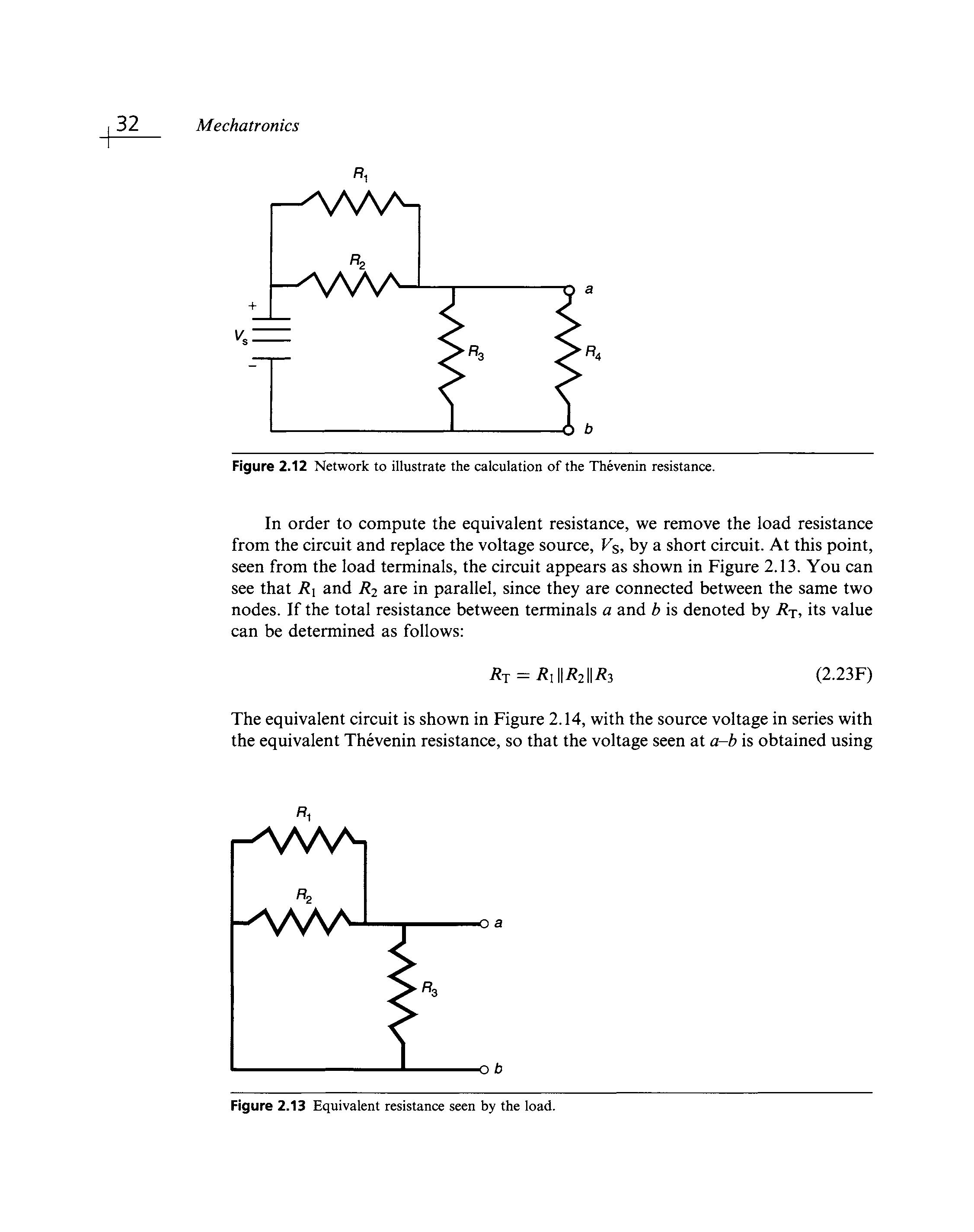
To illustrate the procedure, consider the simple circuit of Figure 2.12; the objective is to compute the equivalent resistance the load i?L 'sees' at port a-b.
Figure 2.12 Network to illustrate the calculation of the Thevenin resistance
In order to compute the equivalent resistance, we remove the load resistance from the circuit and replace the voltage source, Vs, by a short circuit At this point, seen from the load terminals, the circuit appears as shown in Figure 2.13. You can see that R\ and R2 are in parallel, since they are connected between the same two nodes If the total resistance between terminals a and b is denoted by RT, its value can be determined as follows:
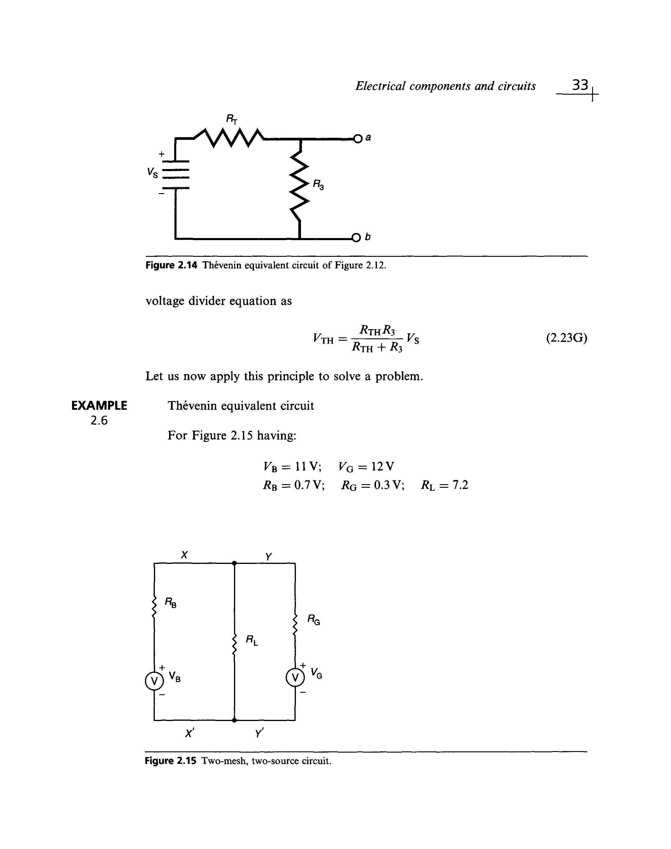
The equivalent circuit is shown in Figure 2.14, with the source voltage in series with the equivalent Thevenin resistance, so that the voltage seen at a-b is obtained using
Figure 2.13 Equivalent resistance seen by the load.
j-AVvA-
Figure 2.14 Thevenin equivalent circuit of Figure 2.12.
voltage divider equation as
Let us now apply this principle to solve a problem.
EXAMPLE Thevenin equivalent circuit
2.6
For Figure 2.15 having:
Figure 2.15 Two-mesh, two-source circuit.
Mechatronics
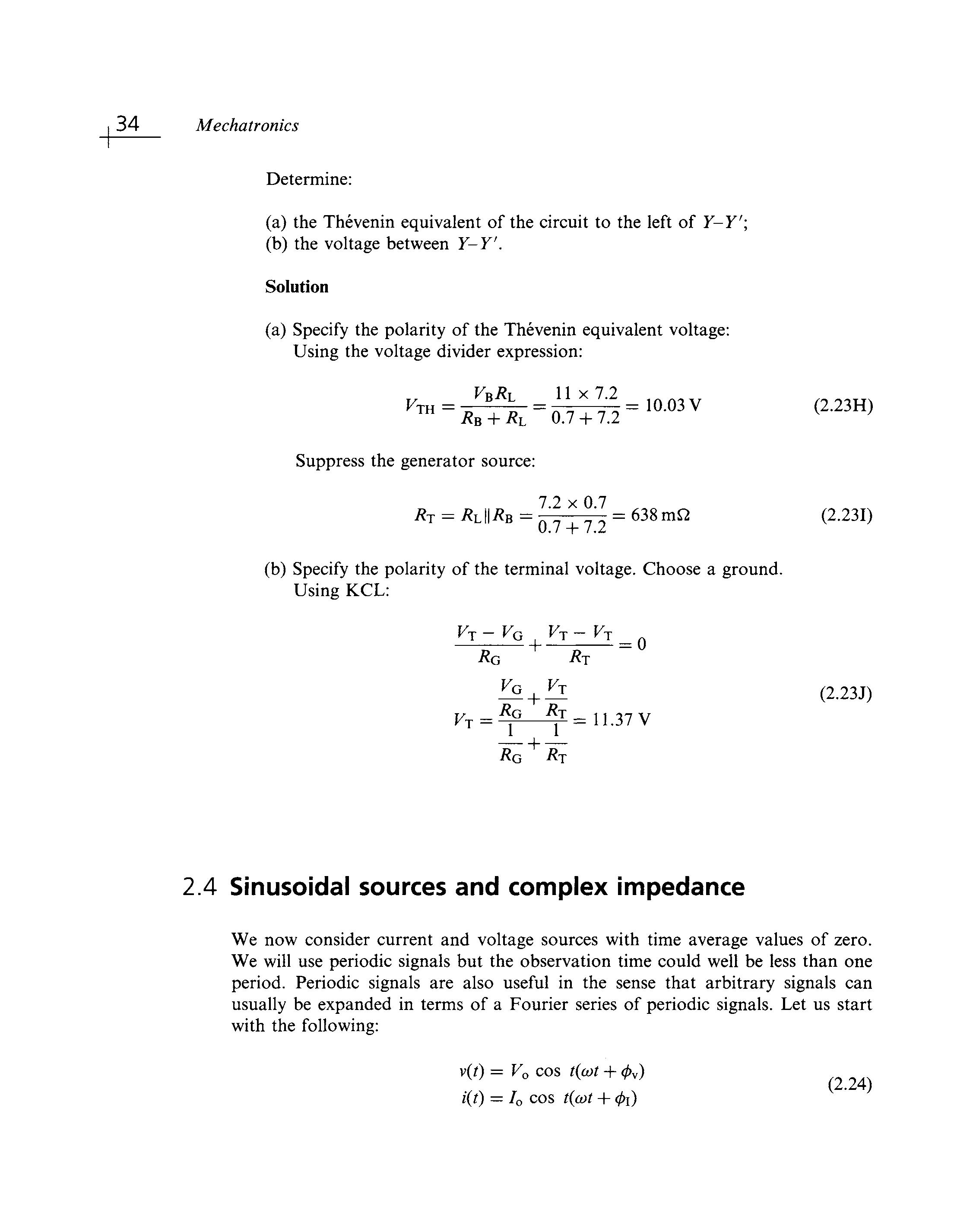
Determine:
(a) the Thevenin equivalent of the circuit to the left of Y-Y'\ (b) the voltage between Y-Y'.
Solution
(a) Specify the polarity of the Thevenin equivalent voltage: Using the voltage divider expression:
Suppress the generator source:
(b) Specify the polarity of the terminal voltage. Choose a ground. Using KCL:
2.4 Sinusoidal sources and complex impedance
We now consider current and voltage sources with time average values of zero. We will use periodic signals but the observation time could well be less than one period. Periodic signals are also useful in the sense that arbitrary signals can usually be expanded in terms of a Fourier series of periodic signals. Let us start with the following:
= V0 cos t(cot + (by) w v ^'
i(i) = I0 cos t(cot + 0i)
Notice that we have now switched to lowercase symbols Lowercase is generally used for a.c. quantities while uppercase is reserved for d.c. values. Now is the time to get into complex notation, often used in electrical and electronic equations, since it will make our discussion easier The above voltage and current signals can be written as
v(t) = V^'^ (2 25) I(t) = / 0 e^' + ^
In order to make things easier, we define one EMF in the circuit to have cp = 0. In other words, we will pick t = 0 to be at the peak of one signal. The vector notation is used to remind us that complex numbers can be considered as vectors in the complex plane Although not so common in physics, in electronics we refer to these vectors as phasors. Hence the reader should now review complex notation. The presence of sinusoidal v(t) or i(t) in circuits will result in an inhomogeneous differential equation with a time-dependent source term The solution will contain sinusoidal terms with the source frequency. The extension of Ohm's law to a.c. circuits can be written as
where co is the source frequency The generalized resistance referred to as the impedance is represented by the letter Z. We can cancel out the common time-dependent factors to obtain
= Z(co)I(co) (2.27)
and hence the power of the complex notation becomes obvious. For a physical quantity we take the amplitude of the real signal as follows
We will now examine each circuit element in turn with a voltage source to deduce its impedance.
2.4.1 Resistive impedance
For a voltage source and resistor, the impedance is equal to the resistance, as expected, given as
2.4.2 Capacitive impedance
For a voltage source and capacitor, the impedance is given as 1 Z = }coC (2.30)
For d.c circuits co = 0 and hence Zc —• oo The capacitor acts like an open circuit (infinite resistance) in a d.c. circuit.
2.4.3 Inductive impedance
For a voltage source and an inductor, the impedance is given as Z = }coL (2.31)
For d.c. circuits co = 0 and hence ZL-> oo. There is no voltage drop across an inductor in a d.c circuit
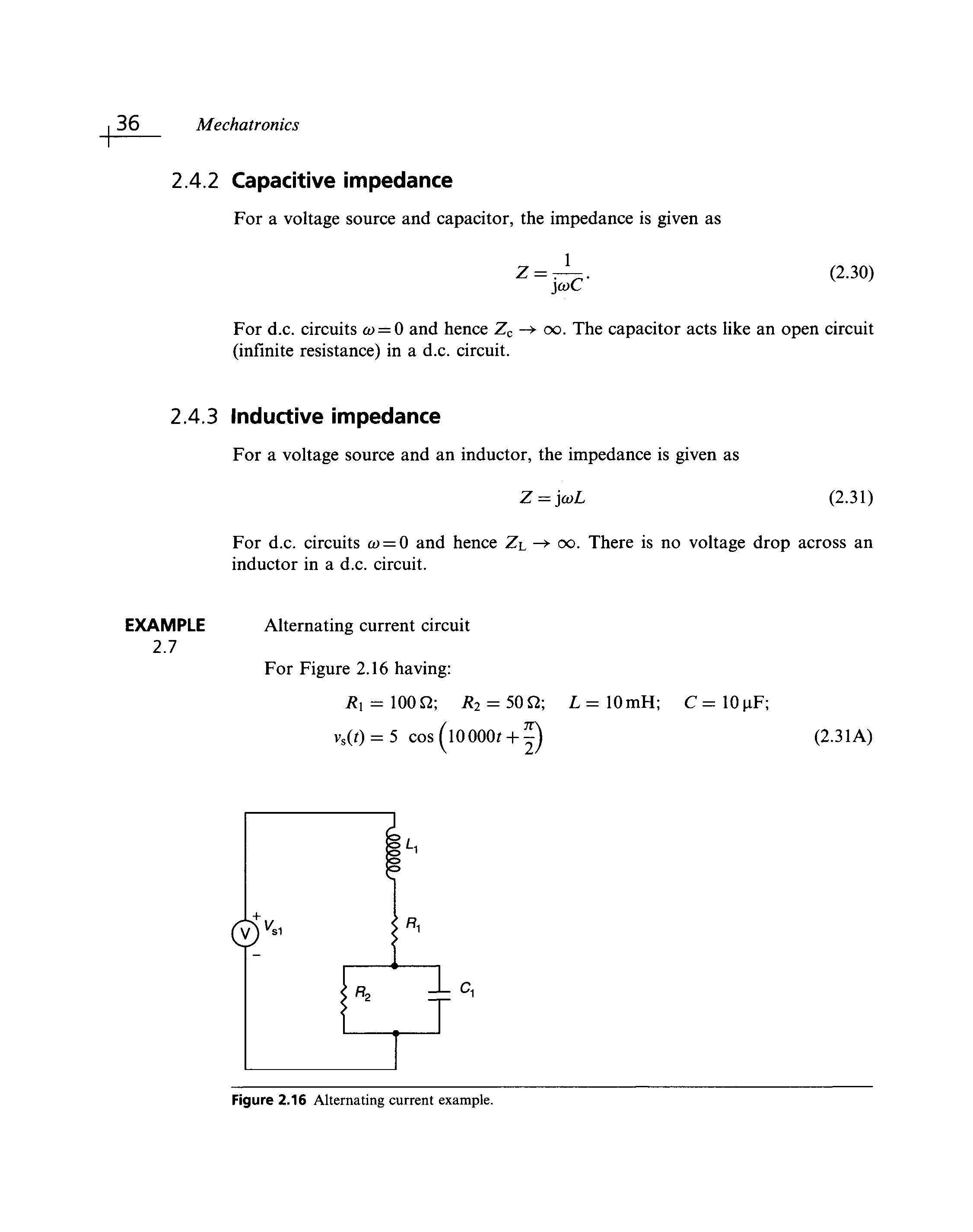
EXAMPLE 2.7
Alternating current circuit
For Figure 2.16 having: Ri = \00Q; R2 = 50Q; L=10mH; C=10|iF; vs(0 = 5 cos(l0000f + ! ) (2.31A)
Figure 2.16 Alternating current example
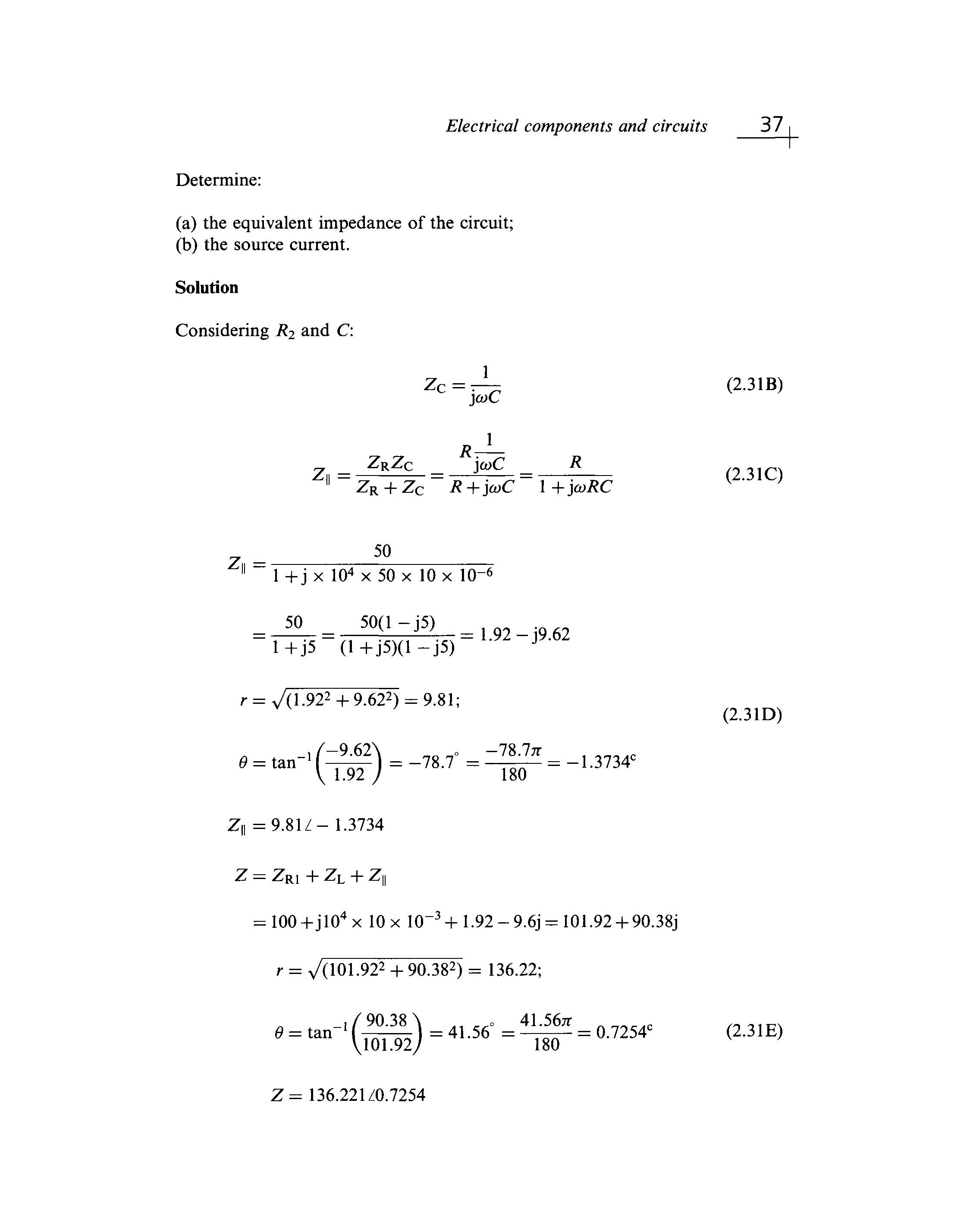
Determine:
(a) the equivalent impedance of the circuit; (b) the source current Solution