MECHATRONICS A Foundation Course
Clarence W. de Silva
Boca Raton London New York
CRC Press is an imprint of the Taylor & Francis Group, an informa business
MATLAB® is a trademark of The MathWorks, Inc. and is used with permission. The MathWorks does not warrant the accuracy of the text or exercises in this book. This book’s use or discussion of MATLAB® software or related products does not constitute endorsement or sponsorship by The MathWorks of a particular pedagogical approach or particular use of the MATLAB® software.
CRC Press
Taylor & Francis Group
6000 Broken Sound Parkway NW, Suite 300
Boca Raton, FL 33487-2742
© 2010 by Taylor and Francis Group, LLC
CRC Press is an imprint of Taylor & Francis Group, an Informa business
No claim to original U.S. Government works
Printed in the United States of America on acid-free paper 10 9 8 7 6 5 4 3 2 1
International Standard Book Number-13: 978-1-4200-8212-8 (Ebook-PDF)
This book contains information obtained from authentic and highly regarded sources. Reasonable efforts have been made to publish reliable data and information, but the author and publisher cannot assume responsibility for the validity of all materials or the consequences of their use. The authors and publishers have attempted to trace the copyright holders of all material reproduced in this publication and apologize to copyright holders if permission to publish in this form has not been obtained. If any copyright material has not been acknowledged please write and let us know so we may rectify in any future reprint.
Except as permitted under U.S. Copyright Law, no part of this book may be reprinted, reproduced, transmitted, or utilized in any form by any electronic, mechanical, or other means, now known or hereafter invented, including photocopying, microfilming, and recording, or in any information storage or retrieval system, without written permission from the publishers.
For permission to photocopy or use material electronically from this work, please access www.copyright.com (http:// www.copyright.com/) or contact the Copyright Clearance Center, Inc. (CCC), 222 Rosewood Drive, Danvers, MA 01923, 978-750-8400. CCC is a not-for-profit organization that provides licenses and registration for a variety of users. For organizations that have been granted a photocopy license by the CCC, a separate system of payment has been arranged.
Trademark Notice: Product or corporate names may be trademarks or registered trademarks, and are used only for identification and explanation without intent to infringe.
Visit the Taylor & Francis Web site at http://www.taylorandfrancis.com
and the CRC Press Web site at http://www.crcpress.com
To Professor Jim A.N. Poo for his friendship and continuous support.
“We live in a society exquisitely dependent on science and technology, in which hardly anyone knows anything about science and technology.”
Carl Sagan
2.4.3
2.5
2.6
2.5.2
2.5.3
2.6.1
2.6.2
2.6.1.1
2.6.1.2
2.6.1.3
2.6.1.4
2.6.1.5
2.6.1.6
2.6.2.1
2.6.2.2
2.6.2.3
2.6.2.4
2.6.3
2.6.3.1
2.6.3.2
2.6.3.3
2.6.3.4
2.6.3.5
2.6.3.6
2.6.3.7 Reluctance .......................................................................................58
2.6.3.8 Inductance .......................................................................................59
2.7 Active Electronic Components ..................................................................................60
2.7.1 Diodes ..............................................................................................................60
2.7.1.1 PN Junctions ...................................................................................60
2.7.1.2 Semiconductors ..............................................................................60
2.7.1.3 Depletion Region ............................................................................61
2.7.1.4 Biasing ..............................................................................................61
2.7.1.5 Zener Diodes ...................................................................................63
2.7.1.6 VVC Diodes .....................................................................................64
2.7.1.7 Tunnel Diodes .................................................................................64
2.7.1.8 PIN Diodes ......................................................................................65
2.7.1.9 Schottky Barrier Diodes ................................................................65
2.7.1.10 Thyristors ........................................................................................65
2.7.2 Transistors .......................................................................................................67
2.7.2.1 Bipolar Junction Transistors .........................................................67
2.7.2.2 Field-Effect Transistors ..................................................................69
2.7.2.3 The MOSFET ...................................................................................70
2.7.2.4 The Junction Field Effect Transistor ............................................71
2.8 Light Emitters and Displays ......................................................................................74
2.8.1 Light-Emitting Diodes...................................................................................75
2.8.2 Lasers ...............................................................................................................76
3.1
3.2
2.8.3
2.9.2
2.9.3
2.9.4
2.9.5
2.9.6
3.2.1
3.2.2
3.2.2.1
3.2.2.2
3.2.2.3
3.2.2.4
3.2.3 Lumped Model of a Distributed System ....................................................95
3.2.3.1 Heavy Spring ..................................................................................96
3.3 Lumped Elements and Analogies ............................................................................98
3.3.1 Across Variables and through Variables ....................................................99
3.3.2 Natural Oscillations ....................................................................................100
3.4 Analytical Model Development ..............................................................................100
3.4.1 Steps of Model Development .....................................................................101
3.4.2 Input–Output Models .................................................................................102
3.4.3 State-Space Models ......................................................................................102
3.4.3.1 Linear State Equations .................................................................102
3.5 Model Linearization .................................................................................................111
3.5.1 Linearization about an Operating Point ...................................................111
3.5.2 Function of Two Variables ..........................................................................113
3.5.3 Reduction of System Nonlinearities..........................................................114
3.5.4 Linearization Using Experimental Operating Curves ...........................120
3.5.4.1 Torque–Speed Curves of Motors ................................................120
3.5.4.2 Linear Models for Motor Control...............................................120
3.6 Linear Graphs ............................................................................................................122
3.6.1 Variables and Sign Convention ..................................................................123
3.6.1.1 Sign Convention ...........................................................................123
3.6.2 Linear Graph Elements ...............................................................................125
3.6.2.1 Single-Port Elements ....................................................................125
3.6.2.2 Two-Port Elements .......................................................................127
3.6.3 Linear Graph Equations ..............................................................................131
3.6.3.1 Compatibility (Loop) Equations .................................................131
3.6.3.2 Continuity (Node) Equations .....................................................132
3.7
3.6.4
3.6.4.1
3.6.4.2
3.6.4.3
3.6.4.4
3.6.5
3.7.1
3.7.2
3.7.3
3.8
3.9
3.10
3.7.2.1
3.7.2.2 Bode Diagram (Bode Plot) and Nyquist Diagram ...................152
3.7.3.1
3.7.3.2
3.8.1
3.8.2
3.9.1
3.9.2
3.9.3
3.10.1
3.11
3.10.2
3.10.3
3.10.1.1 Homogeneous
3.10.1.2
3.10.1.3
3.10.1.4 Stability ..........................................................................................175
3.10.3.1
3.10.3.2
3.10.3.3
3.10.4
3.10.4.1
3.10.4.2
3.10.4.3
3.10.5
3.11.1
3.11.1.1
3.11.1.2
3.11.1.3
3.11.1.4
4.2 Impedance Characteristics ......................................................................................230
4.2.1 Cascade Connection of Devices .................................................................231
4.2.1.1 Output Impedance .......................................................................231
4.2.1.2 Input Impedance ..........................................................................231
4.2.1.3 Cascade Connection.....................................................................232
4.2.2 Impedance Matching...................................................................................234
4.2.3 Impedance Matching in Mechanical Systems .........................................235
4.3 Amplifiers...................................................................................................................237
4.3.1 Operational Amplifier .................................................................................238
4.3.1.1 Use of Feedback in Op-Amps .....................................................241
4.3.2 Voltage and Current Amplifiers ................................................................242
4.3.3 Instrumentation Amplifiers .......................................................................243
4.3.3.1 Differential Amplifier ..................................................................243
4.3.3.2 Common Mode .............................................................................245
4.3.4 Amplifier Performance Ratings .................................................................246
4.3.4.1 Common-Mode Rejection Ratio .................................................247
4.3.4.2 AC-Coupled Amplifiers ...............................................................249
4.3.5 Ground Loop Noise .....................................................................................249
4.4 Filters...........................................................................................................................251
4.4.1 Passive Filters and Active Filters ...............................................................252
4.4.1.1 Number of Poles ...........................................................................253
4.4.2 Low-Pass Filters............................................................................................253
4.4.2.1 Low-Pass Butterworth Filter .......................................................254
4.4.3 High-Pass Filters ..........................................................................................255
4.4.4 Band-Pass Filters ..........................................................................................256
4.4.4.1 Resonance-Type Band-Pass Filters .............................................257
4.4.4.2 Band-Reject Filters ........................................................................257
4.4.5 Digital Filters ................................................................................................258
4.4.5.1 Software and Hardware Implementations ...............................259
4.5 Modulators and Demodulators ...............................................................................260
4.5.1 Amplitude Modulation ...............................................................................262
4.5.1.1 Modulation Theorem ...................................................................263
4.5.1.2 Side Frequencies and Side Bands ...............................................263
4.5.2 Application of Amplitude Modulation .....................................................264
4.5.2.1 Fault Detection and Diagnosis ...................................................266
4.5.3 Demodulation ...............................................................................................267
4.6 Analog-to-Digital Conversion .................................................................................267
4.6.1 Digital-to-Analog Conversion ....................................................................270
4.6.1.1 Weighted Resistor DAC ...............................................................271
4.6.1.2 Ladder DAC...................................................................................272
4.6.1.3 DAC Error Sources .......................................................................274
4.6.2 Analog-to-Digital Conversion ....................................................................276
4.6.2.1 Successive Approximation ADC ................................................276
4.6.2.2 Dual Slope ADC ...........................................................................278
4.6.2.3 Counter ADC ................................................................................280
4.6.2.4 ADC Performance Characteristics .............................................281
4.6.3 Sample-and-Hold Circuitry ........................................................................284
4.6.4 Multiplexers ..................................................................................................285
4.7 Bridge Circuits ...........................................................................................................
5.
5.1
4.7.1
4.7.2
4.7.3 Hardware Linearization of Bridge Outputs.............................................290
4.7.4 Bridge Amplifiers .........................................................................................290
4.7.5 Half-Bridge Circuits.....................................................................................290
4.7.6 Impedance Bridges ......................................................................................291
4.7.6.1
4.7.6.2 Wien-Bridge Oscillator ................................................................293
5.1.1
5.1.2
5.2 Linearity .....................................................................................................................304
5.2.1 Saturation ......................................................................................................305
5.2.2
5.2.3
5.2.4
5.2.5
5.2.6
5.3
5.3.1
5.4 Bandwidth ..................................................................................................................310
5.4.1
5.4.2
5.4.3 Half-Power (or 3 dB) Bandwidth ................................................................311
5.4.4 Fourier Analysis Bandwidth ......................................................................312
5.4.5 Useful Frequency Range .............................................................................312
5.4.6 Instrument Bandwidth................................................................................313
5.4.7 Control Bandwidth ......................................................................................313
5.4.8 Static Gain .....................................................................................................313
5.5 Signal Sampling and Aliasing Distortion .............................................................314
5.5.1 Sampling Theorem ......................................................................................314
5.5.2 Anti-Aliasing Filter ......................................................................................315
5.5.3 Another Illustration of Aliasing ................................................................317
5.6 Bandwidth Design of a Control System .................................................................320
5.6.1 Comment about Control Cycle Time.........................................................320
5.7 Instrument Error Analysis.......................................................................................320
5.7.1 Statistical Representation............................................................................322
5.7.2 Accuracy and Precision...............................................................................322
5.7.3 Error Combination .......................................................................................323
5.7.4 Absolute Error ..............................................................................................325
5.7.5 SRSS Error .....................................................................................................325
5.8 Statistical Process Control........................................................................................328
5.8.1 Control Limits or Action Lines ..................................................................329
5.8.2 Steps of SPC ..................................................................................................329 Problems ................................................................................................................................330
6.2
6.3
6.2.1
6.2.2
6.3.1
6.4
6.3.3
6.3.4
6.3.5
6.3.6
6.3.7
6.3.8
6.3.9
6.4.1
6.4.2
6.4.3
6.5
6.6
6.3.3.1
6.7
6.8
6.5.2
6.5.3
6.5.4
6.6.1
6.3.7.1
6.6.1.1
6.6.1.2
6.6.1.3
6.6.1.4
6.6.1.5
6.6.2
6.7.1
6.7.2
6.8.1
6.8.2
6.8.3
6.8.4
6.8.5
6.9
6.10
6.11
6.12
6.9.1
6.10.1
6.10.2
6.10.3
6.10.4
6.11.1
6.12.1
6.12.2
6.12.3
6.12.3.1
6.12.3.2 Resistance
6.12.3.3
6.12.3.4
6.13 Digital Transducers ...................................................................................................414
6.13.1
6.13.2 Shaft Encoders ..............................................................................................415
6.13.2.1 Encoder Types ...............................................................................415
6.13.3 Incremental Optical Encoder .....................................................................416
6.13.3.1 Direction of Rotation ...................................................................419
6.13.3.2 Hardware Features ......................................................................419
6.13.3.3 Displacement Measurement .......................................................421
6.13.3.4 Digital Resolution .........................................................................421
6.13.3.5 Physical Resolution ......................................................................422
6.13.3.6 Step-Up Gearing ...........................................................................422
6.13.3.7 Interpolation..................................................................................423
6.13.3.8 Velocity Measurement .................................................................424
6.13.3.9 Velocity Resolution.......................................................................424
6.13.3.10 Step-Up Gearing ...........................................................................427
6.13.3.11 Data Acquisition Hardware ........................................................428
6.13.4 Absolute Optical Encoders .........................................................................429
6.13.4.1 Gray Coding ..................................................................................430
6.13.4.2 Code Conversion Logic ...............................................................431
6.13.4.3 Advantages and Drawbacks .......................................................432
6.13.5 Encoder Error ...............................................................................................432
6.13.5.1 Eccentricity Error .........................................................................433
6.14 Miscellaneous Digital Transducers ........................................................................434
6.14.1 Digital Resolvers ..........................................................................................434
6.14.2 Digital Tachometers .....................................................................................435
6.14.3 Hall-Effect Sensors ......................................................................................436
6.14.4 Linear Encoders ...........................................................................................438
6.14.5 Moiré Fringe Displacement Sensors .........................................................439
6.14.6 Binary Transducers ......................................................................................441
6.14.7 Other Types of Sensors ...............................................................................444
6.15
6.15.3
7.3
7.2.3
7.2.4
7.2.5
7.2.6
7.2.6.1
7.2.7
7.3.1
7.3.4
7.3.5
7.3.6
7.3.7
7.3.4.1
7.3.5.1
7.3.5.2
7.3.6.1
7.3.6.2
7.3.6.3
7.3.7.1
7.3.7.2
7.3.7.3
7.3.8
7.3.9
7.3.8.1
7.3.8.2
7.3.9.1
7.3.9.2
8.
7.3.9.3 Motor Sizing Procedure ..............................................................506
7.3.9.4 Inertia Matching ...........................................................................507
7.3.9.5 Drive Amplifier Selection............................................................508
7.4 Induction Motors .......................................................................................................510
7.4.1 Rotating Magnetic Field ..............................................................................511
7.4.2 Induction Motor Characteristics ................................................................512
7.4.3 Torque–Speed Relationship ........................................................................514
7.4.4 Induction Motor Control .............................................................................518
7.4.4.1 Excitation Frequency Control .....................................................518
7.4.4.2 Voltage Control .............................................................................520
7.4.4.3 Field Feedback Control (Flux Vector Drive) .............................523
7.4.5 A Transfer-Function Model for an Induction Motor ..............................523
7.4.6 Single-Phase AC Motors .............................................................................525
7.5 Miscellaneous Actuators ..........................................................................................526
7.5.1 Synchronous Motors ...................................................................................526
7.5.1.1 Control of a Synchronous Motor ................................................527
7.5.2 Linear Actuators ..........................................................................................527
7.5.2.1 Solenoid .........................................................................................527
7.5.2.2 Linear Motors................................................................................529
7.6 Hydraulic Actuators .................................................................................................530
7.6.1 Components of a Hydraulic Control System ...........................................531
7.6.2 Hydraulic Pumps and Motors....................................................................532
7.6.3 Hydraulic Valves ..........................................................................................535
7.6.3.1 Spool Valve ....................................................................................536
7.6.3.2 Steady-State Valve Characteristics .............................................538
7.6.4 Hydraulic Primary Actuators ....................................................................541
7.6.5 The Load Equation.......................................................................................542
7.6.6
7.6.6.1
7.6.7 Constant-Flow Systems ...............................................................................552
7.6.8 Pump-Controlled Hydraulic Actuators ....................................................553
7.6.9 Hydraulic Accumulators.............................................................................553
7.6.10 Pneumatic Control Systems........................................................................554
7.6.10.1 Flapper Valves...............................................................................554
7.6.11 Hydraulic Circuits .......................................................................................557 Problems ................................................................................................................................558
8.2.1
8.2.2.1 Signed Magnitude Representation ............................................582
8.2.2.2 Two’s Complement Representation ...........................................582
8.2.2.3 One’s Complement .......................................................................583
8.2.3
8.2.4
8.2.5 Binary Coded Decimal ................................................................................584
8.2.6 ASCII (Askey) Code .....................................................................................584
8.3 Logic and Boolean Algebra .....................................................................................585
8.3.1 Logic...............................................................................................................585
8.3.1.1 Negation ........................................................................................585
8.3.1.2 Disjunction ....................................................................................585
8.3.1.3 Conjunction ...................................................................................585
8.3.1.4 Implication ....................................................................................586
8.3.2 Boolean Algebra ...........................................................................................587
8.3.2.1 Sum and Product Forms..............................................................588
8.4 Combinational Logic Circuits .................................................................................588
8.4.1 Logic Gates ....................................................................................................588
8.4.2 IC Logic Families .........................................................................................591
8.4.3 Design of Logic Circuits .............................................................................592
8.4.3.1 Multiplexer Circuit .......................................................................593
8.4.3.2 Adder Circuits ..............................................................................593
8.4.3.3 Active-Low Signals ......................................................................594
8.4.4 Minimal Realization ....................................................................................596
8.4.4.1 Karnaugh Map Method ...............................................................596
8.5 Sequential Logic Devices .........................................................................................598
8.5.1
8.5.2 Latch...............................................................................................................600
8.5.3 JK Flip-Flop ...................................................................................................600
8.5.4 D Flip-Flop ....................................................................................................602
8.5.4.1 Shift Register .................................................................................602
8.5.5 T Flip-Flop and Counters............................................................................603
8.5.6 Schmitt Trigger.............................................................................................606
8.6 Practical Considerations of IC Chips......................................................................607
8.6.1 IC Chip Production ......................................................................................607
8.6.2 Chip Packaging ............................................................................................608
8.6.3 Applications ..................................................................................................609
8.7 Microcontrollers ........................................................................................................609
8.7.1 Microcontroller Architecture .....................................................................609
8.7.1.1 Microcontroller Operation ..........................................................610
8.7.2 Microprocessor .............................................................................................611
8.7.2.1 Arithmetic Logic Unit ..................................................................611
8.7.2.2 Program Counter ..........................................................................612
8.7.2.3 Address Register ..........................................................................612
8.7.2.4 Accumulator and Data Register .................................................613
8.7.2.5 Instruction Register .....................................................................613
8.7.2.6 Operation Decoder .......................................................................613
8.7.2.7 Sequencer.......................................................................................613
8.7.3 Memory .........................................................................................................613
8.7.3.1 RAM, ROM, PROM, EPROM, and EEPROM ............................613
8.7.3.2 Bits, Bytes, and Words .................................................................614
8.7.3.3 Volatile Memory ...........................................................................614
8.7.3.4 Physical Form of Memory ...........................................................614
8.7.3.5 Memory Access .............................................................................615
8.7.3.6 Memory Card Design ..................................................................617
9.1
9.2
8.7.4
9.3
8.7.5
8.7.4.1 Microcontroller Pin-Out ..............................................................620
8.7.4.2 Programmed I/O ..........................................................................620
8.7.4.3 Interrupt I/O .................................................................................622
8.7.4.4
8.7.4.5 Handshaking
8.7.4.6
8.7.5.1
8.7.5.2
8.7.5.3 Program
8.7.5.4
8.7.6
9.2.1
9.2.3
9.3.1
9.2.2.1
9.2.3.1
9.3.1.1
9.4 Control Schemes ........................................................................................................649
9.4.1 Feedback Control with PID Action ...........................................................651
9.4.1.1
9.4.2
9.5 Stability .......................................................................................................................656
9.5.1 Routh–Hurwitz Criterion ...........................................................................657
9.5.1.1 Routh Array ..................................................................................658
9.5.1.2 Auxiliary Equation (Zero-Row Problem) .................................659
9.5.1.3 Zero Coefficient Problem ............................................................660
9.5.1.4 Relative Stability ...........................................................................661
9.5.2 Root Locus Method .....................................................................................662
9.5.2.1 Root Locus Rules ..........................................................................664
9.5.2.2 Steps of Sketching Root Locus ...................................................665
9.5.3 Stability in the Frequency Domain ...........................................................668
9.5.3.1 Marginal Stability ........................................................................668
9.5.3.2 The 1, 0 Condition ........................................................................668
9.5.3.3 Phase Margin and Gain Margin ................................................670
9.5.3.4 Bode and Nyquist Plots ...............................................................671
9.6 Advanced Control .....................................................................................................672
9.6.1 Linear Quadratic Regulator Control .........................................................673
9.6.2 Modal Control ..............................................................................................674
9.6.3
9.6.4
9.6.5
9.6.6
9.6.7
9.7 Fuzzy
9.7.1
9.7.2
9.7.3
9.7.4
9.7.5
9.8.1
9.8.2
9.7.3.1
9.7.3.2
9.7.3.3
9.7.3.4
9.7.4.1
10.4
A.4
A.4.2 Rotating Thick Cylinders ............................................................................762
A.4.2.1 Strain Equations ...........................................................................763
A.4.2.2 Stress–Strain (Constitutive) Relations .......................................763
A.4.2.3 Equilibrium Equations ................................................................763
A.4.2.4 Final Result....................................................................................764
A.4.2.5 Temperature Stresses ...................................................................764
A.4.3 Particular Cases of Cylinders .....................................................................764
A.4.3.1 Case 1: Axially Restrained Ends ................................................764
A.4.3.2 Case 2: Thick Pressure Vessel .....................................................765
A.4.3.3 Case 3: Thin Pressure Vessel ......................................................765
A.4.3.4 Case 4: Rotating Cylinder with Free Ends ................................765
A.5 Mohr’s Circle of Plane Stress ...................................................................................766
A.6 Torsion ........................................................................................................................767
A.6.1 Circular Members ........................................................................................767
A.6.2 Torque Sensor ...............................................................................................769
A.7 Beams in Bending and Shear ..................................................................................772
A.7.1 Mohr’s Theorems .........................................................................................772
A.7.2 Maxwell’s Theorem of Reciprocity ............................................................772
A.7.3 Castigliano’s First Theorem ........................................................................773
A.7.4 Elastic Energy of Bending ..........................................................................773
A.8 Open-Coiled Helical Springs ..................................................................................773
A.8.1 Case 1: Axial Load W ..................................................................................773
A.8.2 Case 2: Axial Couple M ...............................................................................775
A.9 Circular Plates with Axisymmetric Loading ........................................................776
A.9.1 Strains ............................................................................................................776
A.9.2 Stresses ..........................................................................................................776
A.9.3 Moments ........................................................................................................776
A.9.4 Equilibrium Equations ................................................................................777
A.9.5 Boundary Conditions ..................................................................................778
A.9.5.1 Fixed Edge .....................................................................................778
A.9.5.2 Simply Supported
A.9.5.3 Partially
B.1 Laplace Transform ....................................................................................................779
B.1.1 Laplace Transforms of Some Common Functions ..................................780
B.1.1.1 Laplace Transform of a Constant ...............................................780
B.1.1.2 Laplace Transform of the Exponential ......................................780
B.1.1.3 Laplace Transform of Sine and Cosine ......................................781
B.1.1.4 Laplace Transform of a Derivative .............................................782
B.1.2 Table of Laplace Transforms .......................................................................783
B.2 Response Analysis ....................................................................................................785
B.3 Transfer Function ......................................................................................................790
B.4 Fourier Transform .....................................................................................................792
B.4.1 Frequency-Response Function (Frequency Transfer Function) ............793
B.5 The s -Plane .................................................................................................................793
B.5.1 An Interpretation of Laplace and Fourier Transforms ...........................794
B.5.2 Application in Circuit Analysis .................................................................794
Appendix C: Probability and Statistics .................................................................................797
C.1 Probability Distribution ...........................................................................................797
C.1.1 Cumulative Probability Distribution Function .......................................797
C.1.2 Probability Density Function .....................................................................797
C.1.3 Mean Value (Expected Value) ....................................................................798
C.1.4 Root-Mean-Square Value ............................................................................798
C.1.5 Variance and Standard Deviation .............................................................798
C.1.6 Independent Random Variables ................................................................799
C.1.7 Sample Mean and Sample Variance ..........................................................800
C.1.8 Unbiased Estimates .....................................................................................800
C.1.9 Gaussian Distribution .................................................................................802
C.1.10 Confidence Intervals....................................................................................803
C.2 Sign Test and Binomial Distribution ......................................................................806
C.3 Least Squares Fit .......................................................................................................808
Appendix D: Software Tools ...................................................................................................813
D.1 Simulink® ...................................................................................................................813
D.2 MATLAB®...................................................................................................................813
D.2.1 Computations ...............................................................................................813
D.2.1.1 Arithmetic .....................................................................................814
D.2.1.2 Arrays.............................................................................................814
D.2.2 Relational and Logical Operations ............................................................815
D.2.3 Linear Algebra ..............................................................................................816
D.2.4 M-Files ...........................................................................................................817
D.3 Control Systems Toolbox ..........................................................................................817
D.3.1 Compensator Design Example...................................................................817
D.3.1.1 Building the System Model .........................................................820
D.3.1.2 Importing Model into SISO Design Tool ..................................820
D.3.1.3 Adding Lead and Lag Compensators .......................................820
D.3.2 PID Control with Controller Tuning .........................................................821
D.3.2.1 Proportional Control ....................................................................821
D.3.2.2 PI Control.......................................................................................821
D.3.2.3 PID Control ...................................................................................824
D.3.3 Root Locus Design Example ......................................................................825
D.4 Fuzzy Logic Toolbox .................................................................................................825
D.4.1 Graphical Editors .........................................................................................828
D.4.2 Command Line–Driven FIS Design ..........................................................828
D.4.3 Practical Stand-Alone Implementation in C ............................................829
D.5 LabVIEW.....................................................................................................................829
D.5.1 Introduction ..................................................................................................830
D.5.2 Some Key Concepts .....................................................................................830
D.5.3 Working with LabVIEW..............................................................................831
D.5.3.1 Front Panel.....................................................................................832
D.5.3.2 Block Diagrams.............................................................................832
D.5.3.3 Tools Palette ..................................................................................834
D.5.3.4 Controls Palette ............................................................................834
D.5.3.5 Functions Palette ..........................................................................834 Index .............................................................................................................................................837
Preface
This is an introductory book on the subject of mechatronics. It can serve as both a textbook and a reference book for engineering students and practicing professionals, respectively. As a textbook, it is suitable for undergraduate or entry-level graduate courses in mechatronics, mechatronic devices and components, sensors and actuators, electromechanical systems, system modeling and simulation, and control system instrumentation.
Mechatronics concerns the synergistic and concurrent use of mechanics, electronics, computer engineering, and intelligent control systems in modeling, analyzing, designing, developing, implementing, and controlling smart electromechanical products. As modern machinery and electromechanical devices are typically being controlled using analog and digital electronics and computers, the technologies of mechanical engineering in such a system can no longer be isolated from those of electronic and computer engineering. For example, in a robotic system or a micromachine, mechanical components are integrated and embedded with analog and digital electronic components and microcontrollers to provide single functional units or products. Similarly, devices with embedded and integrated sensing, actuation, signal processing, and control have many practical advantages. In the framework of mechatronics, a unified approach is taken to integrate different types of components and functions, both mechanical and electrical, in modeling, analysis, design, implementation, and control, with the objective of harmonious operation that meets a desired set of performance specifications in a rather “optimal” manner, resulting in benefits with regard to performance, efficiency, reliability, cost, and environmental impact.
Mechatronics has emerged as a bona fide field of practice, research, and development, and simultaneously as an academic discipline in engineering. Historically, the approach taken in learning a new field of engineering has been to fi rst concentrate on a single branch of engineering, such as electrical, mechanical, civil, chemical, or aerospace engineering, in an undergraduate program and then learn the new concepts and tools during practice, graduate study, or research. Since the discipline of mechatronics involves electronic and electrical engineering, mechanical and materials engineering, and control and computer engineering, a more appropriate approach would be to acquire a strong foundation in the necessary fundamentals from these various branches of engineering in an integrated manner in a single and unified undergraduate curriculum. In fact, many universities in the United States, Canada, Europe, Asia, and Australia have established both undergraduate and graduate programs in mechatronics. This book is focused toward an integrated education and practice as related to electromechanical systems.
Scope of the Book
The book is an outgrowth of my experience in integrating key components of mechatronics into senior-level courses for engineering students, and in teaching graduate and
professional courses in mechatronics and related topics. The material in the book has acquired an application orientation through industrial experience I have gained at organizations such as IBM Corporation, Westinghouse Electric Corporation, Bruel and Kjaer, and NASA’s Lewis and Langley Research Centers. To maintain clarity and the focus and to maximize the usefulness of the book, I have presented the material in a manner that will be convenient and useful to anyone with a basic engineering background, be it electrical, mechanical, aerospace, control, or computer engineering. Case studies, detailed worked examples, and exercises are provided throughout the book. Complete solutions to the end-of-chapter problems are presented in a “Solutions Manual,” which will be available to instructors who take up a detailed study of the book.
The book consists of 10 chapters and 4 appendices. The chapters are devoted to presenting the fundamentals in electrical and electronic engineering, mechanical engineering, control engineering, and computer engineering, which are necessary for forming the foundation of mechatronics. In particular, they cover mechanical components, electrical and electronic components, modeling, analysis, instrumentation, sensors, transducers, signal processing, actuators, control, and system design and integration. The book uniformly incorporates the underlying fundamentals into analytical methods, modeling approaches, and design techniques in a systematic manner throughout the main chapters. The practical application of the concepts, approaches, and tools presented in the introductory chapters are demonstrated through a wide range of practical examples and a comprehensive set of case studies. The background theory and techniques that are not directly useful to present the fundamentals of mechatronics are provided in a concise manner in the appendices. Also, in the Solutions Manual, a curriculum is suggested for an undergraduate degree in mechatronics.
Main Features of the Book
The following are the main features of the book, which will distinguish it from other books on the same topic:
• formatting of the book.
Readability and convenient reference are given priority in the presentation and
Key concepts and formulas developed and presented in the book are summa-
• rized in windows, tables, and lists in a user-friendly format for easy reference and recollection.
• ations and the practice of mechatronics.
A large number of worked examples are included and are related to real-life situ-
Numerous problems and exercises, most of which are based on practical situations
• and applications, and convey additional useful information on mechatronics, are provided at the end of each chapter.
The use of MATLAB
• ®, Simulink®, LabVIEW®, and associated toolboxes are described, and a variety of illustrative examples are provided for their use. Many
problems in the book are cast for solution using these computer tools. However, the main goal of the book is not simply to train the students in the use of software tools. Instead, a thorough understanding of the core and foundation of the subject, as facilitated by the book, will enable the student to learn the fundamentals and engineering methodologies behind the software tools: the choice of proper tools to solve a given problem, interpret the results generated by them, assess the validity and correctness of the results, and understand the limitations of the available tools.
The material is presented in a manner so that users from diverse engineering • backgrounds (mechanical, electrical, computer, control, aerospace, and material) will be able to follow and benefit from it equally.
Useful material that could not be conveniently integrated into the main chapters is • provided separately in four appendices at the end of the book.
An Instructor’s Manual (Solutions Manual) is available, which provides sugges-
• tions for curriculum planning and development, and gives detailed solutions to all the end-of-chapter problems in the book.
A Note to Instructors
A curriculum for a 4-year bachelor’s degree in mechatronics is given in the Instructor’s Manual (Solutions Manual). This book will be suitable as a text for several courses in such a curriculum, as listed below:
Mechatronics
Mechatronic devices and components
Sensors and actuators
Electromechanical systems
System modeling and simulation
Control system instrumentation
Mechatronic system instrumentation
Further material on these topics can be found in the following textbooks (with solutions manuals):
de Silva, C.W., Sensors and Actuators—Control System Instrumentation, CRC Press/Taylor & Francis, Boca Raton, FL, 2007.
de Silva, C.W., Modeling and Control of Engineering Systems, CRC Press/Taylor & Francis, Boca Raton, FL, 2009.
Windows® and Word® are software products of Microsoft ® Corporation, Redmond, WA.
For MATLAB® and Simulink® product information, please contact
The MathWorks, Inc.
3 Apple Hill Drive
Natick, MA, 01760-2098 USA
Tel: 508-647-7000
Fax: 508-647-7001
E-mail: info@mathworks.com
Web: www.mathworks.com
LabVIEW™ is a product of National Instruments, Inc, Austin, TX.
I have personally used these software tools for teaching and for the development of this book.
Vancouver, British Columbia, Canada
Clarence W. de Silva
Acknowledgments
Many individuals have assisted in the preparation of this book, but it is not practical to acknowledge all such assistance here. First, I wish to recognize the contributions, both direct and indirect, of my graduate students, research associates, and technical staff. Particular mention should be made of my PhD student, Roland H. Lang, whose research assistance has been very important. I am particularly grateful to Jonathan W. Plant, senior editor, CRC Press/Taylor & Francis, for his interest, enthusiasm, and strong support throughout the project. Others at CRC Press and its affi liates, in particular, Christine Selvan, Joette Lynch, Anithajohny Mariasusai, Jessica Vakili, and others for their fi ne effort in producing this book. I also wish to acknowledge the advice and support of various authorities in the field—particularly, Professor Devendra Garg of Duke University; Professor Madan Gupta of the University of Saskatchewan; Professor Mo Jamshidi of the University of Texas (San Antonio, Texas); Professors Ben Chen, Tong-Heng Lee, and Kok-Kiong Tan of the National University of Singapore; Professor Maoqing Li of Xiamen University; Professor Max Meng of the Chinese University of Hong Kong; Dr. Daniel Repperger of the U.S. Air Force Research Laboratory; and Professor David N. Wormley of the Pennsylvania State University. Finally, I owe an apology to my wife and children for the unintentional “neglect” that they may have faced during the latter stages of the preparation of this book and am grateful for all their support.
Author
Clarence W. de Silva, PE, fellow ASME, fellow IEEE, fellow Royal Society of Canada, is a professor of mechanical engineering at the University of British Columbia, Vancouver, Canada, and occupies the Tier 1 Canada Research Chair professorship in mechatronics and industrial automation. Prior to this he occupied the Natural Sciences and Engineering Research Council–British Columbia Packers Research Chair in Industrial Automation since 1988. He served as a faculty member at Carnegie Mellon University (1978–1987) and as a Fulbright visiting professor at the University of Cambridge, Cambridge, England (1987–1988).
Professor de Silva received two PhD degrees from the Massachusetts Institute of Technology (1978) and the University of Cambridge, England (1998), and an honorary DEng from the University of Waterloo, Waterloo, Ontario, Canada (2008). Dr. de Silva also occupied the Mobil Endowed Chair professorship in the Department of Electrical and Computer Engineering at the National University of Singapore and the honorary chair professorship of the National Taiwan University of Science and Technology.
Other fellowships include the Fellow Canadian Academy of Engineering, Lilly Fellow, NASA-ASEE Fellow, Senior Fulbright Fellow to Cambridge University, Fellow of the Advanced Systems Institute of BC, Killam Fellow, and Erskine Fellow.
Professor de Silva has received the Paynter Outstanding Investigator Award and Takahashi Education Award, ASME Dynamic Systems & Control Division; Killam Research Prize; Outstanding Engineering Educator Award, IEEE Canada; and the Lifetime Achievement Award, World Automation Congress. He has also received the IEEE Third Millennium Medal; Meritorious Achievement Award, Association of Professional Engineers of BC; Outstanding Contribution Award, IEEE Systems, Man, and Cybernetics Society. He has given 20 keynote addresses.
He has served on 14 journals including IEEE Transactions on Control System Technology; the Journal of Dynamic Systems, Measurement & Control; and Transactions of ASME; editor in chief, the International Journal of Control and Intelligent Systems and the International Journal of Knowledge-Based Intelligent Engineering Systems. Other editorial duties include senior technical editor, Measurements and Control; and regional editor, North America, Engineering Applications of Artificial Intelligence—IFAC International Journal of Intelligent RealTime Automation.
Professor de Silva has published 19 technical books, 18 edited books, 44 book chapters, about 200 journal articles, and over 215 conference papers.
In the areas of research and development, he has been involved in industrial process monitoring and automation, intelligent multi-robot cooperation, mechatronics, intelligent control, sensors, actuators, and control system instrumentation, with funding of about $7 million, as principal investigator, during the past 15 years.
Mechatronic Engineering
Study Objectives
•
•
Introduction to mechatronics
Modeling and design in mechatronics
• Application areas
Mechatronic technologies
• Study of mechatronics
•
1.1 Introduction
The subject of mechatronics concerns the synergistic application of mechanics, electronics, controls, and computer engineering in the development of electromechanical products and systems through an integrated design approach. A mechatronic system will require a multidisciplinary approach for its modeling, design, development, and implementation. In the traditional development of an electromechanical system, the mechanical components and electrical components are designed or selected separately and then integrated, possibly with other components and hardware and software. In contrast, in the mechatronic approach, the entire electromechanical system is treated concurrently in an integrated manner by a multidisciplinary team of engineers and other professionals. Naturally, a system formed by interconnecting a set of independently designed and manufactured components will have a lower level of performance than that of a mechatronic system, which employs an integrated approach for design, development, and implementation. The main reason is straightforward. The best match and compatibility between component functions can be achieved through an integrated and unified approach to design and development, and the best performance is possible through an integrated implementation. Generally, a mechatronic product will be more efficient and cost effective, more precise and accurate, more reliable, more flexible and functional, less mechanically complex, safer, and more environment friendly than a non-mechatronic product requiring a similar level of effort in its development. The performance of a non-mechatronic system can be improved through sophisticated control, but this is achieved at an additional cost of sensors, instrumentation, and control hardware and software, and with added complexity.
Mechatronic products and systems include modern automobiles and aircraft, smart household appliances, medical robots, space vehicles, and office automation devices. In this chapter, the subject of mechatronics is introduced, important issues in modeling, design, and the development of a mechatronic product or system are highlighted, and the associated technology areas and applications are indicated.
1.2 Mechatronic Systems
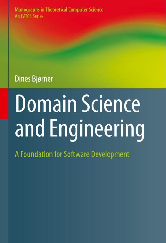
A typical mechatronic system consists of a mechanical skeleton, actuators, sensors, controllers, signal conditioning/modification devices, computer/digital hardware and software, interface devices, and power sources. Different types of sensing, information acquisition, and transfer are involved among all these various types of components. For example, a servomotor, which is a motor with the capability of sensory feedback for accurate generation of complex motions, consists of mechanical, electrical, and electronic components (see Figure 1.1). The main mechanical components are the rotor, stator, and the bearings. The electrical components include the circuitry for the field windings and rotor windings (not in the case of permanent-magnet rotors) and the circuitry for power transmission and commutation (if needed). Electronic components include those needed for sensing (e.g., an optical encoder for displacement and speed sensing and a tachometer for speed sensing). The overall design of a servomotor can be improved by taking a mechatronic approach.
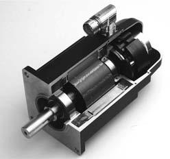
The humanoid robot shown in Figure 1.2a is a more complex and “intelligent” mechatronic system. It may involve many servomotors and a variety of mechatronic components, as is clear from the sketch in Figure 1.2b. A mechatronic approach can greatly benefit the analysis/modeling, design, and development of a complex electromechanical system of this nature.
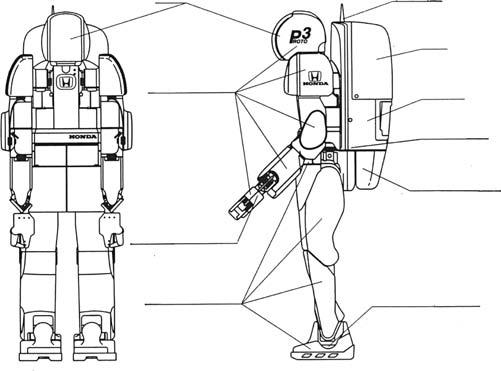
In the computer industry, hard-disk drives (HDD; see Figure 1.3), devices for disk retrieval, access and ejection, and other electromechanical components can considerably benefit from high-precision mechatronics. The impact goes
1.2
1.1
A servomotor is a mechatronic device. (Courtesy of Danaher Motion, Rockford, IL.)
(a) A humanoid robot is a complex and “intelligent” mechatronic system; (b) components of a humanoid robot. (Courtesy of American Honda Motor Co. Inc., Torrance, CA.)
FIGURE
FIGURE
Spindle
Head
1.3
An HDD unit of a computer.
further because digital computers are integrated into a vast variety of other devices and mechatronic applications.
Technology issues of a general mechatronic system are indicated in Figure 1.4. It is seen that they span the traditional fields of mechanical engineering, electrical and electronic engineering, control engineering, and computer engineering. Each aspect or issue within
Modeling, Analysis
Integrated design
Testing and refinement
Sensors and transducers
System development tasks
Controllers
Structural components
Energy sources
Electronics (analog/digital) Actuators
Software
Hydraulic and pneumatic devices
Signal processing
Thermal devices Input/output hardware
Mechanical engineering
FIGURE 1.4
Concepts and technologies of a mechatronic system.
Mechatronic system
Electrical and computer engineering
FIGURE
the system may take a multi-domain character. For example, as noted before, an actuator (e.g., dc servo motor) itself may represent a mechatronic device within a larger mechatronic system such as an automobile or a robot.
The study of mechatronic engineering should include all stages of modeling, design, development, integration, instrumentation, control, testing, operation, and maintenance of a mechatronic system.
1.3 Modeling and Design
A model is a representation of a real system, and the subject of model development (modeling) is important in mechatronics (see Chapter 3). Modeling and design can go hand-inhand in an iterative manner. Of course, in the beginning of the design process, the desired system does not exist. In this context, a model of the anticipated system can be very useful. In view of the complexity of a design process, particularly when striving for an optimal design, it is useful to incorporate system modeling as a tool for design iteration particularly because prototyping can become very costly and time consuming.
In the beginning, by knowing some information about the system (e.g., intended functions, performance specifications, past experience, and knowledge of related systems) and by using the design objectives, it is possible to develop a model of sufficient (low to moderate) detail and complexity. By analyzing and carrying out computer simulations of the model, it will be possible to generate useful information that will guide the design process (e.g., the generation of a preliminary design). In this manner, design decisions can be made and the model can be refi ned using the available (improved) design. This iterative link between modeling and design is schematically shown in Figure 1.5.
It is expected that the mechatronic approach will result in a higher quality of the products and services, improved performance, and increased reliability while approaching some form of optimality. This will enable the development and production of
FIGURE 1.5
Link between modeling and design.
electromechanical systems efficiently, rapidly, and economically. When performing the integrated design of a mechatronic system, the concepts of energy and power present a unifying thread. The reasons are clear. First, in an electromechanical system, ports of power and energy exist that link electrical dynamics and mechanical dynamics. Hence, the modeling, analysis, and optimization of a mechatronic system can be carried out using a hybrid system (or multi-domain system) formulation (a model) that integrates mechanical aspects and electrical aspects of the system. Second, an optimal design will aim for minimal energy dissipation and maximum energy efficiency. There are related implications; for example, greater dissipation of energy will mean reduced overall efficiency and increased thermal problems, noise, vibration, malfunctions, wear and tear, and increased environmental impact. Again, a hybrid model that presents an accurate picture of the energy/power flow within the system will present an appropriate framework for the mechatronic design. (Note: Refer to linear graph models in particular, as discussed in Chapter 3.)
A design may use excessive safety factors and worst-case specifications (e.g., for mechanical loads and electrical loads). This will not provide an optimal design or may not lead to the most efficient performance. Design for optimal performance may not necessarily lead to the most economical (least costly) design, however. When arriving at a truly optimal design, an objective function that takes into account all important factors (performance, quality, cost, speed, ease of operation, safety, environmental impact, etc.) has to be optimized. A complete design process should generate the necessary details for the construction or assembly of the system.
1.4 Mechatronic Design Concept
In a true mechatronic sense, the design of a multi-domain multicomponent system will require the simultaneous consideration and integrated design of all its components, as indicated in Figure 1.4. Such an integrated and “concurrent” design will call for a fresh look at the design process itself and also a formal consideration of information and energy transfer between the components within the system.
In an electromechanical system, there exists an interaction (or coupling) between electrical dynamics and mechanical dynamics. Specifically, electrical dynamics affect the mechanical dynamics and vice versa. Traditionally, a “sequential” approach has been adopted to the design of multi-domain (or mixed) systems such as electromechanical systems. For example, first the mechanical and structural components are designed, next the electrical and electronic components are selected or developed and interconnected, then a computer is selected and interfaced with the system, subsequently a controller is added, and so on. The dynamic coupling between various components of a system dictates, however, that an accurate design of the system should consider the entire system as a whole rather than designing the electrical/electronic aspects and the mechanical aspects separately and sequentially. When independently designed components are interconnected, several problems can arise as follows:
1. When two independently designed components are interconnected, the original characteristics and operating conditions of the two will change due to the loading or dynamic interactions (see Chapter 4).
2. A perfect matching of two independently designed and developed components will be practically impossible. As a result, a component can be considerably underutilized or overloaded, in the interconnected system, both conditions being inefficient and undesirable.
3. Some of the external variables in the components will become internal and “hidden” due to interconnection, which can result in potential problems that cannot be explicitly monitored through sensing and cannot be directly controlled.
The need for an integrated and concurrent design for electromechanical systems can be identified as a primary motivation for the developments in the field of mechatronics.
1.4.1 Coupled Design
An uncoupled design is where each subsystem is designed separately (and sequentially), while keeping the interactions with the other subsystems constant (i.e., ignoring the dynamic interactions). Mechatronic design involves an integrated or “coupled” design. The concept of mechatronic design may be illustrated using an example of an electromechanical system, which can be treated as a coupling of an electrical subsystem and a mechanical subsystem. An appropriate model for the system is shown in Figure 1.6a. Note that the two subsystems are coupled using a loss-free (pure) energy transformer while the losses (energy dissipation) are integral with the subsystems. In this system, assume that under normal operating conditions the energy flow is from the electrical subsystem to the mechanical subsystem (i.e., the electrical subsystem behaves like a motor rather than a generator). At the electrical port that connects to the energy transformer, there exists a current i (a “through” variable) flowing in and a voltage v (an “across” variable) with the shown polarity (the concepts of through and across variables and the related terminology are explained in Chapter 3). The product vi is the electrical power, which is positive out of the electrical subsystem and into the transformer. Similarly, at the mechanical port that comes out of the energy transformer, there exists a torque τ (a through variable) and an angular speed ω (an across variable) with the sign convention indicated in Figure 1.6a. Accordingly, a positive mechanical power ωτ flows out of the transformer and into the mechanical subsystem. The ideal transformer implies that
FIGURE 1.6
(a) An electromechanical system; (b) conventional design.
In a conventional uncoupled design of the system, the electrical subsystem is designed by treating the effects of the mechanical subsystem as a fixed load, and the mechanical subsystem is designed by treating the electrical subsystem as a fixed energy source, as indicated in Figure 1.6b. Suppose that, in this manner, the electrical subsystem achieves an optimal “design index” of Iue and the mechanical subsystem achieves an optimal design index of Ium
Note: The design index is a measure of the degree to which the particular design satisfies the design specifications (design objectives).
When the two uncoupled designs (subsystems) are interconnected, there will be dynamic interactions. As a result, neither the electrical design objectives nor the mechanical design objectives will be satisfied at the levels dictated by Iue and Ium, respectively. Instead, they will be satisfied at lower levels as given by the design indices Ie and Im. A truly mechatronic design will attempt to bring Ie and Im as close as possible to Iue and Ium, respectively. This may be achieved, for example, by minimizing the quadratic cost function:
where D denotes the transformation that represents the design process p denotes information including system parameters that is available for the design
Even though this formulation of the mechatronic design problem appears rather simple and straightforward, the reality is otherwise. In particular, the design process, as denoted by the transformation D, can be quite complex and typically nonanalytic. Furthermore, minimization of the cost function J is by and large an iterative practical scheme and undoubtedly a knowledge-based and nonanalytic procedure. This complicates the process of mechatronic design. In any event, the design process will need the information represented by p.
1.4.2 Mechatronic Design Quotient
Mechatronic systems are complex and require multiple technologies in multiple domains. Their optimal design may call for multiple performance indices. The problem of mechatronic design may be treated as a maximization of a “mechatronic design quotient” or MDQ. In particular, an alternative formulation of the optimization problem given by (1.2) and (1.3) would be the maximization of the MDQ:
subject to (1.3).
Even though Equation 1.4 is formulated for two categories of technologies or devices m and e (and the corresponding indices Ie and Im), the MDQ may be generalized for three or more categories such as: reliability, maintainability, efficiency, cost effectiveness, power and efficiency, size and geometry, control friendliness, and level of intelligence. The
corresponding indices may be qualitative or nonanalytic and may have correlations or interactions. Then, more sophisticated representations (e.g., the use of fuzzy measures) and optimization techniques (e.g., evolutionary computing or genetic programming or GP) may be employed in the design process.
For example, in the use of genetic algorithms (GA) for mechatronic design, we start with a group (population) of initial chromosomes (embryos) where an individual chromosome is one possible design. An individual gene in a chromosome corresponds to an element of information in a design (e.g., system component, connection structure, set of parameters, design attribute). Alleles are possible values of a gene (e.g., available choices for a particular component). The “fitness function” of the GA represents the “value,” “goodness,” or “fitness” of a design. In the present context, the fitness function is the MDQ, which is computable for a given design once the element information of the design is known. Then the problem of design optimization becomes: 12
where, pi is the ith design aspect.
The strength and applicability of the MDQ approach stem from the possibility that the design process may be hierarchically separated. Then, an MDQ may be optimized for one design layer involving two more technology groups in that layer before proceeding to the next lower design layer where each technology group is separately optimized by considering several technology/component groups within that group together with an appropriate MDQ for that lower-level design problem. For example, an upper layer may optimize the actuator type for the particular application (e.g., hydraulic, dc, induction, stepper; see Chapter 7) with an appropriate MDQ. The next lower level may optimize the motor selection (e.g., select a motor from an available set of dc motors) with another MDQ. In this manner, a complex design optimization may be achieved through several design optimizations at different design levels. The fi nal design may not be precisely optimal, yet intuitively adequate for practical purposes; say in a conceptual design.
1.4.3 Design Evolution
Traditionally, the online monitoring of responses/outputs of a system may be used to detect and diagnose the faults and malfunctions (existing or impending) of a system. We believe that such monitoring may also be used to improve the design of an existing mechatronic system. In particular, just like how a health monitoring system can pinpoint a defective component in a system, it should be possible for the same system to at least identify the possible regions (sites) of design weakness in the system. This is the premise of the approach for “design evolution”, as outlined below.
A model of the existing system (whose design needs to be improved) and evolutionary computing (GP) may facilitate the approach of “evolutionary” design improvement through online monitoring. A possible framework for implementing this approach is indicated in Figure 1.7.
The relevant steps are as follows:
1. Develop a model of the existing system.
2. Establish (using a machine health monitoring system and an expert system) which aspects or segments of the original system (and its model) may be modified/improved using information monitored from the system. These will provide “modifiable sites” for the existing system/model.
Interface (for users, domain experts, engineers, etc.)
System model (linear graph)
Optimization scheme (GP)
Structure of a system for evolutionary design.
Existing mechatronic system
Machine health monitoring system
Expert system (engineering knowledge of system)
Performance function (MDQ)
Design improvements
3. Formulate a performance function to represent the “goodness” of the design. This is the MDQ.
4. Use an optimization method (GP) to evolve the model so as to maximize the performance function.
5. Implement, in the existing system, the design changes represented by the evolved model.
The optimization scheme will gradually improve the original model of the system so as to produce better performance (as judged by the MDQ). This will require the comparison of the monitored response of the original system and the simulated response of the model as it evolves (improves), with respect to the MDQ. In Figure 1.7, in addition to the initial model of the system, the evolutionary computing approach, and online monitoring, we have shown an expert system as well for “intelligent” decision making associated with design/model improvement. This expert system may be generated from the knowledge/ expertise of the existing system, its design, and engineering know how.
1.5 Evolution of Mechatronics
Mechanical engineering products and systems that employ some form of electrical engineering principles and devices have been developed and used since the early part of the twentieth century. These systems included the automobile, electric typewriter, aircraft, and elevator. Some of the power sources used in these systems were not necessarily electrical, but there were batteries and/or a conversion of thermal power into electricity through
FIGURE 1.7
generators. These “electromechanical” systems were not “mechatronic” systems because they did not use an integrated approach characterizing mechatronics for their analysis, design, development, and implementation.
Rapid advances in electromechanical devices and systems were possible particularly due to developments in control engineering, which began for the most part in the early 1950s, and still more rapid advances in digital computer and communication as a result of integrated circuit (IC) and microprocessor technologies, starting from the late 1960s. With these advances, engineers and scientists felt the need for a multidisciplinary approach to design and hence a “mechatronic” approach. In 1969, Yasakawa Electric in Japan was the fi rst to coin the term mechatronics, for which the company obtained a trademark in 1972. Subsequently, in 1982, the company released the trademark rights. Even though a need for mechatronics was felt even in those early times, no formal discipline or educational programs existed for the engineers to be educated and trained in this area. The research and development activities mainly in automated transit systems and robotics in the 1970s and the 1980s undoubtedly paved the way for the evolution of the field of mechatronics. With today’s sophisticated technologies of mechanics and materials, analog and digital electronics, sensors, actuators, controllers, electromechanical design, and microelectromechanical systems (MEMS) with embedded sensors, actuators, and microcontrollers, the field of mechatronics has attained a high degree of maturity. Now many universities around the world offer undergraduate and graduate programs in mechatronic engineering, which have become highly effective and popular among students, instructors, employees, and employers alike.
1.6 Application Areas
The application areas of mechatronics are numerous and involve those that concern multidomain (mixed) systems and particularly electromechanical systems. These applications may involve the following:
1. Modifications and improvements to conventional designs by using a mechatronic approach
2. The development and implementation of original and innovative mechatronic systems
In either category, the applications may employ sensing, actuation, control, signal conditioning, component interconnection and interfacing, and communication, generally using tools of mechanical, electrical, electronic, computer, and control engineering. Some important areas of application are indicated below.
Transportation is a broad area where mechatronic engineering has numerous applications. In ground transportation, particularly automobiles, trains, and automated transit systems use mechatronic devices. They include airbag deployment systems, antilock braking systems (ABS), cruise control systems, active suspension systems, and various devices for monitoring, toll collection, navigation, warning, and control in intelligent vehicular highway systems (IVHS). In air transportation, modern aircraft designs with advanced materials, structures, electronics, and control benefit from the concurrent and
integrated approach of mechatronics to develop improved designs of fl ight simulators, fl ight control systems, navigation systems, landing gear mechanisms, traveler comfort aids, and the like.
Manufacturing and production engineering is another broad field that uses mechatronic technologies and systems. Factory robots (for welding, spray painting, assembly, inspection, and so on), automated guided vehicles (AGVs), modern computer-numerical control (CNC) machine tools, machining centers, rapid (and virtual) prototyping systems, and micromachining systems are examples of mechatronic applications. High-precision motion control is particularly important in these applications.
In medical and health care applications, robotic technologies for patient examination, surgery, rehabilitation, drug dispensing, and general patient care are being developed and used. Mechatronic technologies are being applied for patient transit devices, various diagnostic probes and scanners, beds, and exercise machines.
In a modern office environment, automated filing systems, multifunctional copying machines (copying, scanning, printing, FAX, and so on), food dispensers, multimedia presentation and meeting rooms, and climate control systems incorporate mechatronic technologies.
In household applications, home security systems, robotic caregivers and helpers, robotic vacuum cleaners, washers, dryers, dishwashers, garage door openers, and entertainment centers use mechatronic devices and technologies.
The computer industry can considerably benefit from mechatronics. The impact goes further because digital computers are integrated into a vast variety of other devices and applications.
In civil engineering applications, cranes, excavators, and other machinery for building, earth removal, mixing, and so on will improve their performance by adopting a mechatronic design approach.
In space applications, mobile robots such as NASA’s Mars exploration Rover, spacestation robots, and space vehicles are fundamentally mechatronic systems.
It is noted that there is no end to the type of devices and applications that can incorporate mechatronics. In view of this, the traditional boundaries between engineering disciplines will become increasingly fuzzy, and the field of mechatronics will grow and evolve further through such merging of disciplines.
1.7 Study of Mechatronics
Mechatronics is a multidisciplinary field that is concerned with the integrated modeling, analysis, design, manufacture, control, testing, and operation of smart electromechanical products and systems. Hence, one should not use a “compartmentalized” approach in studying this field. Specifically, rather than using a conventional approach to learning standard subjects separately in a disjointed manner, they need to be integrated into a common “mechatronics” framework, along with other specialized subjects.
The study of mechatronics requires a good foundation of such core subjects as mechanics, electronics, modeling, control, signal processing and conditioning, communication, and computer engineering, and specialized subjects like electrical components, mechanical components, sensors and transducers, instrumentation, drives and actuators, intelligent control, interfacing hardware, software, testing, performance evaluation, and cost-benefit