LIFE CYCLE COST ANALYSIS OF NATM USING ANN by IRJET Journal

LIFE CYCLE COST ANALYSIS OF NATM USING ANN

Mayur Jadhav1 , Dr. Madhulika Sinha2

1ME Student, Department of Civil Engineering, Pillai HOC College of Engineering and Technology, Rasayani University of Mumbai

2 Department of Civil Engineering, Pillai HOC College of Engineering and Technology, Rasayani University of Mumbai ***

ABSTRACT

The New Austrian Tunneling Method (NATM) is a widely adopted tunneling technique known for its flexibility and costeffectivenessinvariousgeotechnicalconditions.However,thecomplexityofNATMconstructionprocessesandthevariability ofgeologicalfactorsmakeaccuratecostestimationchallenging.ThisstudyfocusesonconductingacomprehensiveLifeCycle Cost Analysis (LCCA) of NATM projects by integrating Artificial Neural Networks (ANN) as a predictive modeling tool. LCCA evaluates the total cost of a project over its entire lifespan, including initial construction, maintenance, and operation, providing a holistic economic assessment. ANN, with its ability to model complex nonlinear relationships and learn from historical data, is utilized to predict the life cycle costs more accurately than traditional methods. The research involves collecting extensive data from completed NATM tunneling projects, including geological parameters, construction variables, andcostelements.Thisdata isusedtotrainandvalidatetheANN model,enabling ittopredictcostoutcomesundervarying conditionseffectively.TheresultsdemonstratethatANNcansignificantlyenhancetheprecisionofcostforecasting,facilitating betterdecision-makingandbudgetplanning.Moreover,theintegrationofLCCAwithANNsupportsstakeholdersinoptimizing resourceallocationandmitigatingfinancialrisksthroughoutthetunnel'soperationallife.Thisstudycontributestothefieldby offering an innovative approach that combines geotechnical engineering with advanced machine learning techniques to improveeconomicevaluationsofcomplextunnelingprojects,promotingsustainableinfrastructuredevelopment.

1. INTRODUCTION

This study explores the integration of Artificial Neural Networks (ANN) into the Life Cycle Cost (LCC) analysis of the New Austrian Tunneling Method (NATM), a widely adopted approach in tunnel construction due to its flexibility and adaptability acrossdiversegeologicalsettings.ThesuccessofNATMhingesonmeticulousplanningandeffectivecostcontrol,makingLCC analysis essential. LCC analysis assesses all expenditures associated with a project over its entire lifespan, from design and constructiontooperationandmaintenance[1].Itenablestheidentificationoflong-termcost-efficientstrategiesbyaccounting forinitialinvestments,futurerepairs,andoperationalexpenses.Intunnelconstruction,suchcomprehensiveevaluationhelps stakeholders in choosing the most economically viable solutions without compromising safety or project requirements[2]. Traditional methods of LCC analysis, however, often fall short in capturing the complexity and uncertainties inherent in tunnelingprojects.Toovercomethis,thestudyincorporatesArtificial Neural Networksasapowerful computational method toenhance prediction accuracyanddecision-makingcapabilities.ANNsare well-suitedtoprocessvasthistorical data,detect complex patterns, and forecast future costs based on various influencing parameters like geological conditions, construction practices, and material choices. Their ability to adapt and learn enables a more realistic and responsive cost model[3]. By employing ANN in LCCanalysisfor NATM,thisresearchaimsto developa smart, data-driven framework for costestimation and optimization[4]. This approach not only improves accuracy but also empowers engineers and project managers to minimize financial risks, optimize resources, and ensure adherence to safety standards. The synergy between ANN and traditionalcostanalysismarksasignificantstepforwardinmodernizingthefinancialplanningandmanagementoftunneling infrastructure.

2. LITERATURE REVIEW

Recent developments in Life Cycle Cost Analysis (LCCA) across various construction and infrastructure domains reflect a growingemphasisoncombiningtraditionalcostestimationmethodswithadvancedcomputationaltechnologies.Forinstance underlinetheimportance of Environmental Product Declarations(EPDs) asfoundational tosustainablebuilding assessment, withLifeCycleAssessment(LCA)playingacentralrole[5].Theirglobalstudyrevealed27keychallengesinimplementingLCA forEPDs,categorizedintosevengroups,includingdataquality,methodologicallimitations,andtechnologicalconstraints.The

International Research Journal of Engineering and Technology (IRJET) e-ISSN: 2395-0056

Volume: 12 Issue: 06 | Jun 2025 www.irjet.net

p-ISSN: 2395-0072

researchhighlightstheurgentneedforhigh-qualitydataandbettertoolstoenhanceLCAreliability,whichdirectlyimpactsthe credibility of EPDs. Similarly demonstrated how Artificial Neural Networks (ANNs) could be used to build a cost model for roadtunnels[6].Byanalyzingcostcomponentsovera75-yearhorizon,theirmodel,appliedtothe EnaticOdors Motorwayin Greece, offered infrastructure managers a precise tool for financial forecasting and planning. ANN-based models are increasinglybeingusedinfieldswherecostaccuracyandadaptabilitytodynamicvariablesarecrucial.applieddynamicLCCA in heritage site conservation through the MONUREV V2 software, showcasing how scenario simulation can inform balanced cultural and economic decisions[7]. compared ANN and regression models for LCC prediction during the early design phase, revealing ANN’s superior accuracy where early-stagedata isminimal[8]. Aleksandra Murkowski et al.(2022) reinforced this trendbyreviewingliteratureonintegratingEnvironmentalLifeCycleCosting(ELCC)withMachineLearning(ML),concluding thatMLenhancestheprecisionandsustainabilityofprojectdecisions. MeanwhilebridgedBIMwithLCCAusingaRevitplugin,empoweringdesignerstoperformreal-timescenarioanalysisthatincludesoperationalandmaintenancefactors further promotinginformedandsustainablebuildingdesigndecisions[9].

ThescopeofANNapplicationsinLCCAextendstoindustrialsystemsandpublicinfrastructure.focusedonpumpingsystems, comparing healthy and faulty states using a hybrid SVM-HMM model[10]. Their AI-based approach enabled early fault detection and significant energy cost savings. noted that LCA and LCCA are underutilized in geotechnical engineering and called for improved frameworks to assist engineers in minimizing life cycle costs[11]. analyzed LCCA in transportation infrastructure,advocatingfortheinclusionofsocialandusercosts,despitequantificationchallenges[12].Thesefindingsecho the work of who evaluated green building projects in Indonesia using LCCA and identified long-term environmental and economic benefits, despite higher upfront costs. proposed replacing simulation-based LCCA with Deep Neural Networks (DNNs) in asset management systems, significantly reducing computational time and enhancing decision-making for large infrastructuredatasets[13].

In tunneling-specific contexts, several studies contribute valuable insights[14]. introduced an ANN and Cost Significant Item (CSI) framework to simplify LCCA in construction, achieving high estimation accuracy in case studies[15]. applied machine learning with geophones in tunneling projects to automate documentation and optimize predictive maintenance[16] proposed a tunnel data schema for NATM using BIM-compatible IFC extensions, helping digitize tunnel design elements[17] addressed the challenge of managing large datasets from NATM tunnel monitoring through a big-data-enabled data service system, improving planning and resource use. developed a planning-stage model using case-based reasoning to estimate environmentalloadsintunnelconstruction,outperformingtraditionalmethodsinaccuracy[18].Thesestudiesemphasizethe increasingdemandfordigitaltoolsthatmanagedatacomplexityandimprovedecisionsupportinNATM-basedtunneling.

3. RESEARCH METHOD

Life Cycle Cost Analysis (LCCA) has become an essential tool for evaluating the long-term economic performance of infrastructure projects. When applied to tunneling projects utilizing the New Austrian Tunneling Method (NATM), LCCA becomes even more crucial due to the method’s inherent complexities, including variable geological conditions, diverse constructiontechniques,andlong operational lifespans[19]. Traditionally,estimatingthecosts associated with suchprojects hasbeenchallenging.However,theintegrationofArtificialNeuralNetworks(ANN)intoLCCApresentsamodern,data-driven solutionthatsignificantlyimprovespredictiveaccuracyanddecision-making[20].ANNmodels,capableoflearningfromlarge sets of historical data, offer the ability to recognize hidden patterns in cost-related factors ranging from excavation and materialusagetolaborandenvironmentalconditions.BytrainingANNwithreal-worldNATMprojectdata,wecananticipate not only initial construction costs but also long-term expenses such as maintenance, energy consumption, and rehabilitation efforts[21]. Furthermore, the synergy between ANN and tools like ANSYS simulations used for finite element analysis allowsthemodeltoincorporatebothempiricaldataandstructuralbehaviorinsights,enablingacomprehensiveandrealistic approach to cost forecasting[22]. This integration facilitates optimized resource allocation, identification of key cost drivers, andenhancedriskmitigation,ultimatelycontributingtothefinancialsustainabilityofNATMtunnelingprojects.

International Research Journal of Engineering and Technology (IRJET) e-ISSN: 2395-0056

Volume: 12 Issue: 06 | Jun 2025 www.irjet.net p-ISSN: 2395-0072

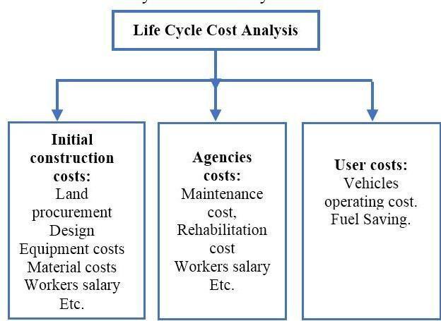
3.1 Methodology and Economic Indicators in LCCA

The methodology for conducting a Life Cycle Cost Analysis in NATM projects using ANN involves several structured steps. Initially, costs related to construction and maintenance are estimated using the Net Present Value (NPV) method, guided by standardssuchasIRCSP-30(2009).Thisapproachinvolvescalculatingthe presentvalueofall costs andbenefitsacross the project’s lifecycle, adjusting for time using discount rates[23]. The four primary steps include estimating initial construction costs, ongoing maintenance, road user costs, and conducting a comprehensive life-cycle cost and benefit analysis using ANN. Tosupporteconomicevaluation,severalindicatorsareemployed,includingNPV,Cost-BenefitRatio(B/C),EquivalentUniform AnnualCosts(EUAC),andInternalRateofReturn(IRR).Eachhasuniqueapplicabilitybasedonprojectscope,decision-making level,andeconomiccontext.Forinstance,incaseswithequalbenefitsacrossalternatives,NPVisthemosteffectiveindicator for comparing differing cost scenarios. NPV’s additive nature simplifies computation by focusing solely on differential costs The economic analysis framework helps decision-makers determine how capital investments weigh against future expenditures,andwhichanalysismethodismostsuitedfortheagency’sgoals[24] Throughthislens,theLCCAmethodology notonlyquantifiescostsbutsupportsstrategicplanningandinvestmentdecisions.

3.2 Data Collection and ANN Model Development

A successful ANN model for LCCA depends heavily on the quality and comprehensiveness of historical data collected from NATM projects. This includes data on construction, operational, maintenance, and rehabilitation costs. Construction data covers excavation, labor, materials, machinery, and unforeseen costs due to geological surprises. Operational costs relate to energy consumption, utilities, and staffing, while maintenance and rehabilitation data focus on regular and major upkeep efforts[25].Additionally,geologicaldata suchasrocktypes,stability,andgroundwaterpresence profoundlyaffectstunnel behaviorandcosts.Othercrucialdataincludesmaterialusage,laborcosts,andenvironmentalconditionsliketemperatureand seismic activity. These diverse data points are obtained from project reports, cost estimation documents, sensor-based monitoring systems, and real-time construction data. Once data is collected, ANN model development involves identifying input variables (e.g., geological factors, excavation techniques, construction methods) and output variables (e.g., total cost, maintenance cost). The network architecture is built with input, hidden, and output layers. ReLU is typically chosen as the activationfunctionforitsefficiencyinhandlinglargedatasets[26].Themodelistrainedusingbackpropagation,whereerrors betweenpredictedandactualoutputsareminimizedthroughiterativeweightadjustments.ThisenablestheANNtoeffectively modelthecomplexrelationshipswithinNATMprojectcostcomponents.

3.3 Model Validation, Testing, and Practical Application

AfterdevelopingtheANNmodel,rigorousvalidationandtestingareessentialtoensureitsreliabilityandapplicabilityin realworld NATM projects[27]. The dataset is typically split into training, validation, and test sets. The training set teaches the model to understand cost patterns, while the validation set helps refine parameters and prevent overfitting. The final evaluationisdoneusingthetestsettoensurethatthemodelgeneralizeswelltonewdata[28].Tofurtherimproverobustness,

International Research Journal of Engineering and Technology (IRJET) e-ISSN: 2395-0056

Volume: 12 Issue: 06 | Jun 2025 www.irjet.net

p-ISSN: 2395-0072

k-foldcross-validationisemployed,wheredataisdividedintomultiplesubsetsandusedinvariouscombinationsfortraining and validation[29]. This enhances the model’s generalization capability and reduces the risk of bias from any single data segment. Performance metrics such as Mean Squared Error (MSE) and R-squared (R²) are used to assess the model’s predictive accuracy. A low MSE and high R² indicate that the model accurately captures the underlying relationships in the data. Ultimately, a well-trained ANN model enables precise forecasting of NATM project costs throughout their lifecycle, supporting better financial planning, design evaluation, and risk management. This modern approach transforms how tunneling projects are assessed economically, promoting long-term sustainability and operational efficiency in the infrastructuresector[30]

4. RESULT AND DISCUSSION

The provided data presents a comprehensive analysis of the annual maintenance costs, life cycle expenses, and predictive modelingoftunnelswithbothrigidandflexiblepavementsovera30-yearhorizon.Utilizingartificialneuralnetworks(ANNs), the study models maintenance cost predictions and evaluates their accuracy through performance metrics such as mean squared error (MSE) and correlation coefficients (R-values). The ANN architectures involve single hidden layers processing input data to forecast multi-dimensional outputs, reflecting the complex relationships in maintenance cost dynamics influencedbyinflationanddiscountrates.

Cost analyses reveal that while rigid pavements incur higher initial expenses, they become more cost-effective than flexible pavementsbeyondthebreak-evenpointaround2030,withatotallifecyclecostadvantageofapproximately4.24%by2048. The data also highlights the significance of discounting future costs at a 12% rate, showing that early investment dominates the net present value (NPV). Predictive models demonstrate strong accuracy in long-term forecasting, particularly for rigid pavements,despitesomeunderestimationofearlyvolatility.Additionally,trainingcurvesandvalidationplotsemphasize the balancebetweenfittingaccuracyandavoidingoverfittingthroughearlystopping. Overall,theintegrationofmachinelearning with economic analysis offers valuable insights for infrastructure planning, indicating that rigid pavement tunnels may provide better economic returns over time despite higher upfront costs, supported by robust predictive modeling to guide maintenanceschedulingandbudgeting.

4.1 Annual maintenance for Tunnel + Rigid Tunnel

Theprovidedimageshowsasimplefeedforwardneuralnetworkarchitecturewithonehiddenlayer.Theinputlayerhasone nodewithavalueof33.Thisinputisfedintothehiddenlayer,whichconsistsof10neurons.Eachneuroninthehiddenlayer applies a weighted sum (represented by "W") and bias ("b") followed by an activation function (indicated by the curve symbol). The processed outputs from the hidden layer then flow into the output layer, which has 33 neurons. Similar operations occur in the output layer weighting, bias addition, and activation. The final output layer produces a 33dimensionaloutputvector.Thisnetworkislikelyusedforregressionorclassificationtaskswheretheinputandoutputsizes areexplicitlydefined.

Figure no.1: Annual maintenance for Tunnel + Rigid Tunnel

International Research Journal of Engineering and Technology (IRJET) e-ISSN: 2395-0056

Volume: 12 Issue: 06 | Jun 2025 www.irjet.net p-ISSN: 2395-0072

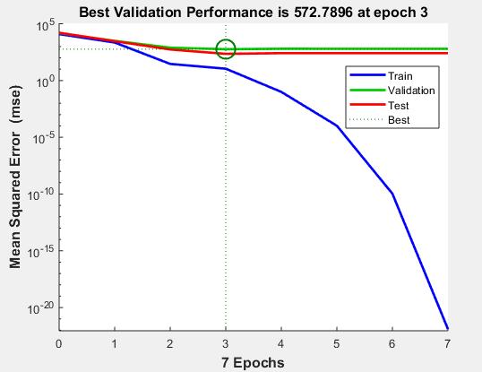
The image shows a plot of Mean Squared Error (MSE) against epochs for training, validation, and testing phases of a model. Theplotislogarithmiconthey-axis.Ithighlightsthebestvalidationperformanceatepoch3,withavalueof572.7896.Atthis epoch,thevalidation error(greenline) reachesits minimum,indicating optimal model performancewithoutoverfitting.The training error (blue line) continuously decreases, showing the model’s learning progress, while the test error (red line) remains steady, closely matching validation error. A green circle marks the best validation point, and a vertical dashed line emphasizes epoch 3. This graph helps to decide the stopping point during training to avoid overfitting while ensuring generalization.ThebestepochisidentifiedbythelowestvalidationMSE,supportingmodelselectioninmachinelearning.

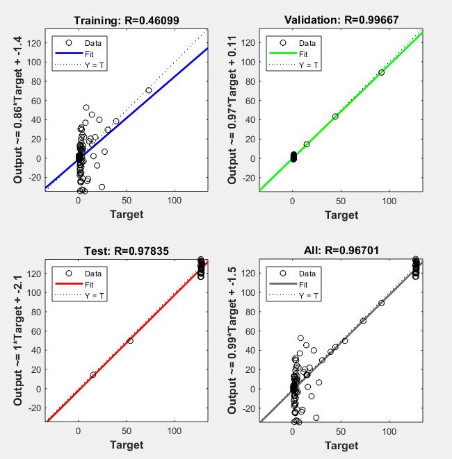
The image presents regression analysis results for a predictive model evaluated on training, validation, test, and combined datasets. The correlation coefficients (R-values) indicate the model's performance: Training (R = 0.46099) shows moderate correlation, while Validation (R = 0.99667) and Test (R = 0.97835) show very high correlation, implying strong predictive

Figure no.2: Best Validation

Figure no.3: Best Trainig, Validation and Test

International Research Journal of Engineering and Technology (IRJET) e-ISSN: 2395-0056

Volume: 12 Issue: 06 | Jun 2025 www.irjet.net p-ISSN: 2395-0072

accuracy on unseen data. The overall dataset has an R-value of 0.96701, confirming good model generalization. The plots depictfittedlinescloselyfollowingtheidealline(Y=T)forvalidationandtestsets,whereastrainingdatashowsmorescatter, suggestingsomeunderfittingornoise.

Figure no.4: ANN prediction of Discounted Cost

ThegraphshowstheANN(ArtificialNeuralNetwork)predictionofdiscountedcostsovertime,from2015to2050.They-axis represents the discounted cost in crores, while the x-axis represents the years. The blue line with circles shows the actual discountedcostvalues,andtheredlinewithstarsrepresentsthepredictedvaluesbytheANNmodel.

Initially, the actual cost fluctuates significantly, peaking around 2020 at about 75 crores, then rapidly drops to near zero by 2023.Thepredictedvaluesstarthighataround45croresin2015andgraduallydecline,aligningwithactualvaluesnearzero around2025.From2025onwards,bothactualandpredictedcostsremainlow,oscillatingslightlyaroundzerowithpredicted valuescloselymatchingactualcosts,showingthemodel'saccuracyinlong-termforecasting.

ThisplotindicatesthattheANNmodeleffectivelycapturesthetrendandmagnitudeofdiscountedcostsovertime,particularly excellinginthelong-termpredictionswherevaluesstabilizenearzero.

International Research Journal of Engineering and Technology (IRJET) e-ISSN: 2395-0056

Volume: 12 Issue: 06 | Jun 2025 www.irjet.net p-ISSN: 2395-0072

4.2 Annual maintenance for Tunnel + Flexible Tunnel

Figure no.5: Hidden and Output Layer

The image depicts a simple neural network architecture with one hidden layer and one output layer. The input layer has 33 nodes, which feed into a hidden layer containing 10 nodes. Each node in the hidden layer has weights (W) and biases (b) applied,followedbyanactivationfunction.Theoutputfromthehiddenlayerthenpassestotheoutputlayer,whichconsistsof 33nodes,eachalsowithweights,biases,andanactivationfunction,producingafinaloutputof33nodes.

This structure is similar to the annual maintenance cost table for Tunnel + Rigid Pavement shown. The table calculates the annualmaintenancecostsanddiscountedvaluesoveryears,reflectingadetailedprocesslikethestepwisetransformationin the neural network. Both represent a systematic progression one through layers of computation (neural network) and the otherthroughyearsofmaintenancecostsconsideringinflationanddiscounting,ultimatelysummarizingthenetpresentvalue overtimeforthecivilconstructionandmaintenancecosts.

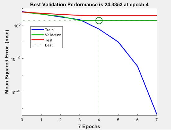
Figure no.6: Best Validation Performance

Thegraphshowsthemeansquarederror(MSE)trendsfortraining,validation,andtestdatasetsover7epochs,withthebest validation performance achieved at epoch 4 (MSE ≈ 24.3353). Initially, all three errors start similarly but diverge as epochs progress.Thetrainingerror(blueline)decreasessignificantlyafterepoch4,indicatingthemodelfitsthetrainingdatabetter. However, validation (green) and test (red) errors remain relatively flat and higher, suggesting possible overfitting. The best validationerrorismarkedwithdottedlinesandagreencircleatepoch4.Thisearlystoppingpointbalancestrainingaccuracy andgeneralization. Thelogarithmicscaleofthey-axis emphasizesthe rapid decline in training errorcompared tovalidation and test errors. The figure highlights that although training error reduces drastically, validation and test errors plateau, indicatingthatcontinuingtrainingbeyondepoch4maynotimprovemodelgeneralization.

International Research Journal of Engineering and Technology (IRJET) e-ISSN: 2395-0056

Volume: 12 Issue: 06 | Jun 2025 www.irjet.net p-ISSN: 2395-0072

Figure no.7: Best Trainig, Validation and Test

The table presents a life cycle cost comparison between tunnels with flexible pavement and those with rigid pavement, factoring ina 5%inflation rateanda 12%discountrate.Initially,in2017, theconstructioncost ofrigidpavementtunnels is higher by 3.06% compared to flexible pavement tunnels, with cumulative costs of 13.77 and 13.36 respectively. Over the years,cumulativecosts for bothtypesincrease,butflexiblepavement remainscheaperuntil theyear2030,whichmarksthe break-even point where costs nearly equalize at approximately 126.00 for rigid and 126.39 for flexible pavement. After this point, flexible pavement costs surpass those of rigid pavement, rising to 132.35 by 2048 compared to 126.73 for rigid pavement. This indicates that, over a 30-year span, rigid pavement proves more cost-effective, being cheaper by 4.24%, highlightingitslong-termeconomicadvantagedespitehigherinitialcosts.

Figure no.8: Gradient and Validation checks

Thegivenimageshowsthe trainingprogressofa machinelearningmodel over six epochsthroughthreeplots. Thefirstplot displays the gradient magnitude, which decreases significantly from around 10^5 to near 10^-5, indicating that the model's parametersarestabilizingandthetrainingisconverging.Thesecondplotshowsthelearningrate(mu),whichalsodecreases steadilyfromroughly10^-5to10^-7,suggestingthattheoptimizationalgorithmisreducingstepsizestofine-tunethemodel

International Research Journal of Engineering and Technology (IRJET) e-ISSN: 2395-0056

Volume: 12 Issue: 06 | Jun 2025 www.irjet.net p-ISSN: 2395-0072

carefully. The third plot represents validation checks (val fail), increasing linearly from 0 to 6, implying that the model is failing validation at each epoch, signaling potential overfitting or poor generalization. Overall, the decreasing gradient and learningrateshowthatthe trainingisprogressing,but thecontinuousvalidationfailuresindicatethatthemodelmaynotbe improvingintermsofvalidationaccuracy,requiringadjustmentsintrainingormodeldesign.

no.9: Best Validation Performance

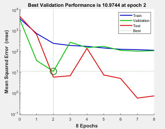
Theplotshowsthemeansquarederror(MSE)performanceofamodelduringtraining,validation,andtestingover8epochs. The vertical axis is logarithmic, displaying MSE values ranging from 0.1 to 10,000, while the horizontal axis represents the number of epochs. The blue line (Train) shows a steady decrease in error but stabilizes around 100. The green line (Validation)decreasesrapidlyinitially,reachingthelowesterrorofapproximately10.97atepoch2,highlightedbyavertical dotted line and a circled point. After epoch 2, validation error fluctuates, indicating potential overfitting. The red line (Test) startshighbutdramaticallydropstobelow1byepoch7,indicatingimprovedtestperformance.Thelegendclarifiesthecolor coding and the best validation point. The best validation performance at epoch 2 signifies the model’s optimal point before overfitting,withMSEaround10.9744,guidingmodelselectionforbalancingaccuracyandgeneralization.

Figure

Figure no.10: ANN Prediction of Discounted cost

International Research Journal of Engineering and Technology (IRJET) e-ISSN: 2395-0056

Volume: 12 Issue: 06 | Jun 2025 www.irjet.net p-ISSN: 2395-0072

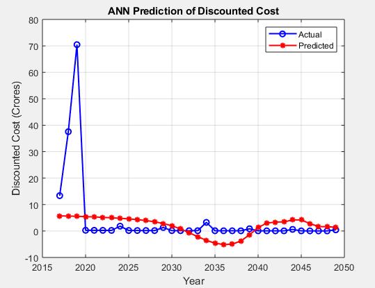
The graph titled "ANN Prediction of Discounted Cost" compares actual and predicted discounted costs (in crores) over time from 2015 to 2050. The blue line with circles represents the actual costs, while the red line with dots shows the predicted costs by an Artificial Neural Network (ANN). Initially, from 2015 to around 2020, actual costs exhibit sharp fluctuations, peaking near 70 crores, whereas predicted costs remain relatively stable around 5-6 crores. Post-2020, actual costs drop significantly and stabilize close to zero, showing minor fluctuations until 2050. The predicted costs gradually decrease from about 5 crores, dip below zero near 2035, and then slowly rise again, aligning more closely with actual values toward 2050. Overall, the ANN model captures the trend but underestimates early volatility and shows smoother predictions throughout. This comparison highlights the model’s strength in trend prediction but also its limitations in capturing sharp real-world fluctuations.

Figure no.11: Cost After Inflation

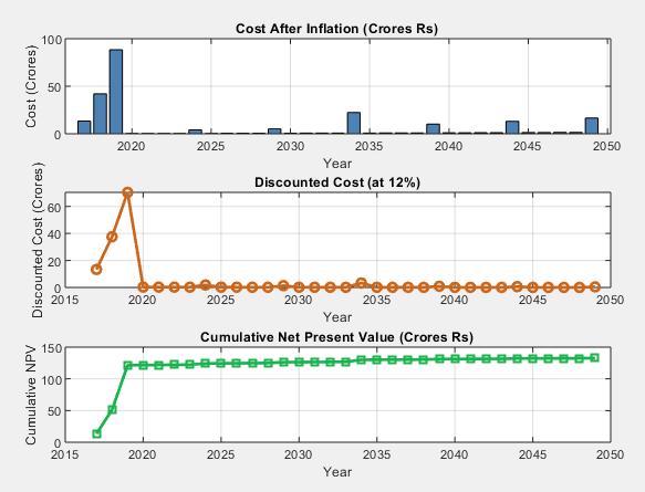
The image presents three related financial plots over the years from 2015 to 2050, focusing on cost and value adjustments consideringinflationanddiscountrates.Thetopplotshowsthe"CostAfterInflation"incroresofrupees,indicatingthatcosts aresignificantlyhigherintheinitialyears(2018-2020),withapeakaround90crores,followedbymuchsmallercostsspread outsporadicallyinlateryears.Themiddleplotdepictsthe"DiscountedCost(at12%),"whereinitialcostspeaksharplyaround 2018-2020 but quickly diminish, reflecting the present value of future costs discounted at a 12% rate, making later costs almostnegligibleinvalue.Thebottomplotillustratesthe"CumulativeNetPresentValue(NPV),"whichstartslowbutsharply risesaround2018-2020toapproximately140croresandthenplateaus,indicating thatmostvalueisaccumulatedearly,and later costs or benefits have minimal impact on the total NPV. Overall, the charts show early high costs with major financial impactandminimallong-termdiscountedcosts,emphasizingtheimportanceofinitialinvestmentsindeterminingnetvalue.

International Research Journal of Engineering and Technology (IRJET) e-ISSN: 2395-0056

Volume: 12 Issue: 06 | Jun 2025 www.irjet.net p-ISSN: 2395-0072

Comparative Analysis

Figure no.12: Training and Test

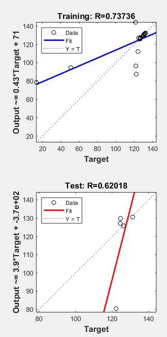
The image displays two scatter plots illustrating the relationship between predicted outputs and target values for a model during training and testing phases. The top plot, labeled "Training: R=0.73736," shows data points scattered around a blue fitted line representing the model’s predictions. The closer the points are to this line, the better the fit. The dotted line representsthe ideal scenariowherepredicted outputequalsthetarget(Y=T). The R-valueof0.73736indicatesa moderate positive correlation during training, meaning the model predictions reasonably align with actual targets, though some variability exists. The bottom plot, labeled "Test: R=0.62018," shows test data with points scattered around a red fitted line, butthislinedivergesmorefromtheidealdottedline.TheR-valueof0.62018indicatesaweakercorrelationinthetestphase, suggestingthemodel’spredictivepowerdecreasesonunseendata.Thisdifferencebetweentrainingandtestingperformance indicatespotentialoverfittingorlimitationsingeneralizationcapability.

International Research Journal of Engineering and Technology (IRJET) e-ISSN: 2395-0056

Volume: 12 Issue: 06 | Jun 2025 www.irjet.net p-ISSN: 2395-0072

Figure no.13:ANN Performance Matrix

Thegraphdepictsthetraining,validation,andtestmeansquarederror(MSE)over9epochsforamachinelearningmodel.The verticalaxisislogarithmic,showingtheMSEvalues,whilethehorizontalaxisrepresentsthenumberofepochs.Theblueline indicatesthetrainingerror, whichsteadilydecreasesovertime, reflectingthe model’simprovingfittothe trainingdata.The red line shows the test error, which follows a similar downward trend. The green line represents validation error, which decreases initially but rises slightly after epoch 3, indicating potential overfitting. The plot highlights the best validation performance of 34.7127 MSE, achieved at epoch 3, marked by vertical and horizontal dotted lines. This epoch is crucial because the validation error is minimized, signifying the optimal balance between underfitting and overfitting. The graph helps in selecting the best epoch for early stopping to ensure generalization on unseen data, avoiding training beyond the pointwherevalidationerrorincreases.

Figure no.14:Training States

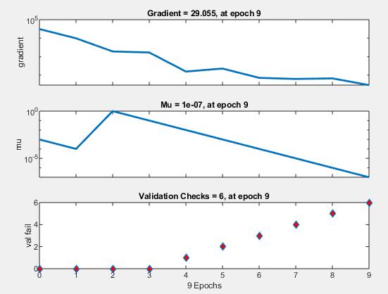
The image shows three line plots depicting the training progress of a machine learning model over 9 epochs. The top plot tracksthe gradient, whichstartsveryhigh(around 10^5)and decreases significantlyby epoch 9 toabout 29.055,indicating thatthemodelisconvergingastheupdatesbecomesmaller.Themiddleplotdisplaysthelearningrateparameter"Mu,"which initially increases to 10^-4 but then steadily decreases to 10^-7 by epoch 9, showing an adaptive adjustment to control the

International Research Journal of Engineering and Technology (IRJET) e-ISSN: 2395-0056

Volume: 12 Issue: 06 | Jun 2025 www.irjet.net p-ISSN: 2395-0072

stepsizeduringtraining.Thebottomplotshowsthevalidationfailures("valfail"),whichremainzeroforthefirstthreeepochs butthenstartincreasinglinearlyfromepoch4to9,reaching6atepoch9.Thissuggeststhatthemodelisencounteringmore validation errors as training progresses, possibly due to overfitting or increased difficulty in improving validation performance.Overall,theplotsindicatedecreasinggradientsandlearningratewithrisingvalidationerrorsatepoch9.

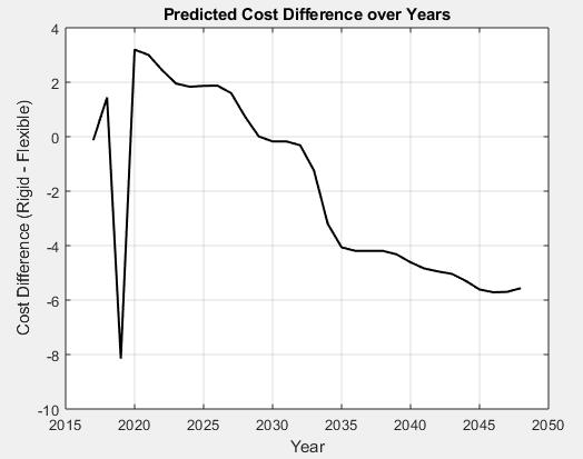
The graph titled "Predicted Cost Difference over Years" illustrates the projected cost difference between rigid and flexible options from 2015 to 2050. The y-axis represents the cost difference (Rigid - Flexible), while the x-axis shows the years. Initially,around2015,thecostdifferenceisslightlypositive,indicatingrigidoptionsarecostlier.However,asharpdip occurs around 2018, showing a significant negative difference of about -8, meaning flexible options were more expensive then. Following this, the cost difference rises dramatically, peaking around 2019-2020 with rigid options costing roughly 3 units more. After 2020, the cost difference steadily declines, crossing zero around 2030 and becoming increasingly negative. By 2050, the cost difference stabilizes near -5.5, implying flexible options become more cost-effective over time. This trend suggests a future economic advantage in using flexible solutions compared to rigid ones, likely due to advancements or cost reductionsinflexibletechnology.

Figure no.14: Predicted Cost Difference over years

Figure no.15: Comparative Predicted NPV

International Research Journal of Engineering and Technology (IRJET) e-ISSN: 2395-0056

Volume: 12 Issue: 06 | Jun 2025 www.irjet.net p-ISSN: 2395-0072

The graph compares the predicted cumulative Net Present Value (NPV) in crores of rupees for rigid and flexible pavements over a period from 2015 to 2050. Both pavement types show a rapid increase in NPV from 2015 to around 2020, with rigid pavementreachingapproximately125croresRsandflexiblepavementslightlylowerbutcloselytrailing.After2020,theNPVs for both pavements plateau, indicating a stabilization in predicted returns. However, flexible pavement continues to show a marginal increase beyond 2020, reaching around 135 crores Rs by 2050, whereas rigid pavement remains almost flat just above125croresRs.Thissuggeststhatflexiblepavementmayofferslightlyhigherlong-termeconomicbenefitscomparedto rigidpavement.Overall,whilebothtypesyieldsignificantreturnsearlyon,flexiblepavementisprojectedtooutperformrigid pavementinthelongrunintermsofcumulativepredictedNPV.

ThegraphdepictsthecumulativeNetPresentValue(NPV)forflexiblepavementovertime,comparingactualversuspredicted values from 2015 to 2050. The Y-axis shows the cumulative NPV in crores of rupees, while the X-axis represents the years. BoththeactualandpredictedNPVvaluesstartlowaround2015butrapidlyincreaseuntil2020,reachingaround120crores. After2020,theNPVvaluesgraduallyriseandstabilizearound130crores.TheactualflexiblepavementNPVisrepresentedby greencircles connected witha solidline,whilethepredictedNPVisshownasa dashedmagenta line.Theclosealignmentof the two lines indicates that the predicted NPV closely matches the actual NPV values throughout the period, reflecting a reliablepredictionmodelforflexiblepavementinvestmentreturnsovertime.

Figure no.16: Flexible Pavement

Figure no.16: Rigid Pavment

International Research Journal of Engineering and Technology (IRJET) e-ISSN: 2395-0056

Volume: 12 Issue: 06 | Jun 2025 www.irjet.net p-ISSN: 2395-0072

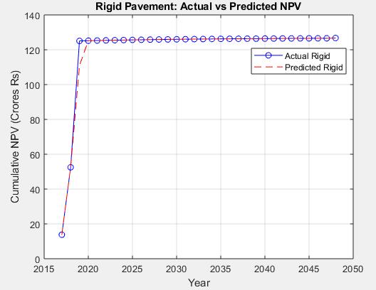
The graph titled "Rigid Pavement: Actual vs Predicted NPV" compares the cumulative Net Present Value (NPV) of rigid pavement over time, from 2015 to 2050. The vertical axis represents the cumulative NPV in Crores of Rupees, while the horizontalaxismarkstheyears.Twolinesareplotted:thebluelinewithcirclesshowstheactualNPV,andthereddashedline showsthepredictedNPV.Bothlinesbeginatalowvaluein2015, risesharplyuntil2020,reachingapproximately130Crores Rs, and then plateau, remaining steady until 2050. The close overlap of the actual and predicted lines indicates a strong agreementbetweenthemodel’spredictionandtheactualobserveddata.Thissuggeststhatthepredictionmodelfortherigid pavement’s NPV is highly accurate in forecasting long-term financial outcomes. The stability in NPV after 2020 indicates no furthersignificantfinancialchangesexpectedinthepavement’svalueoverthefollowingdecades.

5. CONCLUSION

The life cycle cost analysis (LCCA) of the New Austrian Tunneling Method (NATM) using Artificial Neural Networks (ANN) provides a robust framework for evaluating the economic efficiency and sustainability of tunnel construction projects over their entire lifespan. NATM, known for its adaptability to varying geological conditions and its reliance on the surrounding rock for support, presents complex cost implications due to dynamic factors such as excavation methods, support systems, maintenance requirements, and operational conditions. By integrating ANN into LCCA, this study demonstrates an advanced approachtopredictandoptimizecostparameters,therebyenhancingdecision-makingintheearlydesignandplanningstages. ANNmodels,trainedonhistoricalprojectdata,canidentifypatternsandcorrelationsthattraditionalanalyticalmethodsmight overlook.This enablesa morepreciseestimationoftotal lifecyclecosts,incorporatingdirectconstruction expenses,indirect costs,futuremaintenance,andpotential risks.TheapplicationofANNnotonlyimprovestheaccuracyofcostforecastingbut alsosupportsscenarioanalysis,allowingstakeholderstoevaluatealternativedesignsandconstructionstrategiesundervaried economic and environmental conditions. The research concludes that the combination of NATM and ANN-based LCCA significantly improves the efficiency, reliability, and transparency of cost management in tunnel projects. It empowers engineersandprojectmanagerswitha predictivetooltomitigatefinancial risksandoptimizeresourceallocation,ultimately contributingtomorecost-effectiveandsustainableinfrastructuredevelopment.Thestudyrecommendsfurtherexplorationof hybrid AI models and continuous data collection to enhance predictive capabilities and adapt to evolving construction technologies.

REFERENCES

[1] K. Petroutsatou, A. Maravas, and A. Saramourtsis, “A life cycle model for estimating road tunnel cost,” Tunnelling and Underground Space Technology,vol.111,p.103858,May2021,doi:10.1016/j.tust.2021.103858.

[2] F.Davies,L.Moutinho,andB.Curry,“ATMuserattitudes:aneuralnetworkanalysis,” Marketing Intelligence & Planning, vol.14,no.2,pp.26–32,Apr.1996,doi:10.1108/02634509610110778.

[3] A. Qazi, H. Fayaz, A. Wadi, R. G. Raj, N. A. Rahim, and W. A. Khan, “The artificial neural network for solar radiation predictionanddesigningsolarsystems:asystematicliteraturereview,” Journal of Cleaner Production,vol.104,pp.1–12, Oct.2015,doi:10.1016/j.jclepro.2015.04.041.

[4] M. Rafie and F. Samimi Namin, “Prediction of subsidence risk by FMEA using artificial neural network and fuzzy inference system,” International Journal of Mining Science and Technology, vol. 25, no. 4, pp. 655–663, Jul. 2015, doi: 10.1016/j.ijmst.2015.05.021.

[5] O. I. Olanrewaju, A. O. Bello, M. A. Semiu, and S. A. Mudashiru, “Critical barriers to effective communication in the constructionindustry:evidencefromNigeria,” International Journal of Construction Management,vol.25,no.7,pp.783–801,May2025,doi:10.1080/15623599.2024.2362018.

[6] K. Petroutsatou, A. Maravas, and A. Saramourtsis, “A life cycle model for estimating road tunnel cost,” Tunnelling and Underground Space Technology,vol.111,p.103858,May2021,doi:10.1016/j.tust.2021.103858.

[7] E. Hromada, “Real Estate Insights on Mortgage Rates, Apartment Prices, and Rentals in Czech Republic,” IJOES, vol. 13, no.1,pp.13–29,May2024,doi:10.52950/ES.2024.13.1.002.

International Research Journal of Engineering and Technology (IRJET) e-ISSN: 2395-0056

Volume: 12 Issue: 06 | Jun 2025 www.irjet.net p-ISSN: 2395-0072

[8] K. W. Seo et al., “Comparative genetic characterisation of third-generation cephalosporin-resistant Escherichia coli isolatedfromintegratedandconventionalpigfarminKorea,” Journal of Global Antimicrobial Resistance,vol.34,pp.74–82,Sep.2023,doi:10.1016/j.jgar.2023.06.010.

[9] N.Mcneil-AyukandA.Jrade,“AnIntegratedBuildingInformationModeling(BIM)andCircularEconomy(CE)Modelfor the Management of Construction and Deconstruction Waste Based on Construction Methods,” OJCE, vol. 14, no. 02, pp. 168–195,2024,doi:10.4236/ojce.2024.142009.

[10] N. Dutta, K. Palanisamy, P. Shanmugam, U. Subramaniam, and S. Selvam, “Life Cycle Cost Analysis of Pumping System through Machine Learning and Hidden Markov Model,” Processes, vol. 11, no. 7, p. 2157, Jul. 2023, doi: 10.3390/pr11072157.

[11] I.Samuelsson,J.Spross,andS.Larsson,“Integratinglife-cycleenvironmentalimpactandcostsintogeotechnicaldesign,” Proceedings of the Institution of Civil Engineers - Engineering Sustainability, vol. 177, no. 1, pp. 19–30, Feb. 2024, doi: 10.1680/jensu.23.00012.

[12] R.S.Hamid,A.Abror, S.M. Anwar, andA. Hartati, “The roleofsocial mediainthepolitical involvementof millennials,” SJME,vol.26,no.1,pp.61–79,May2022,doi:10.1108/SJME-08-2021-0151.

[13] AliAsgharPilehvar,“Spatial-geographicalanalysisofurbanizationinIran,” Humanit Soc Sci Commun,vol.8,no.1,p.63, Mar.2021,doi:10.1057/s41599-021-00741-w.

[14] A. A. Alqahtani, “Teachers’ perceptions of principals’ motivating language and public school climates in Kuwait,” Management in Education,vol.29,no.3,pp.125–131,Jul.2015,doi:10.1177/0892020615584104.

[15] I. Hartl, M. Sorger, K. Hartl, B. J. Ralph, and I. Schlögel, “Passive seismic monitoring in conventional tunnelling – An innovative approach for automatic process recognition using support vector machines,” Tunnelling and Underground Space Technology,vol.137,p.105149,Jul.2023,doi:10.1016/j.tust.2023.105149.

[16] I. Hartl, M. Sorger, K. Hartl, B. J. Ralph, and I. Schlögel, “Passive seismic monitoring in conventional tunnelling – An innovative approach for automatic process recognition using support vector machines,” Tunnelling and Underground Space Technology,vol.137,p.105149,Jul.2023,doi:10.1016/j.tust.2023.105149.

[17] K. T. Peter et al., “Using High-Resolution Mass Spectrometry to Identify Organic Contaminants Linked to Urban StormwaterMortalitySyndromeinCohoSalmon,” Environ. Sci. Technol.,vol.52,no.18,pp.10317–10327,Sep.2018,doi: 10.1021/acs.est.8b03287.

[18] J.-H.Lee et al.,“Transgenicexpressionofaratiometricautophagyprobespecificallyinneuronsenablestheinterrogation ofbrainautophagy in vivo,” Autophagy,vol.15,no.3,pp.543–557,Mar.2019,doi:10.1080/15548627.2018.1528812.

[19] J.Lai,J.Qiu,Z.Feng,J.Chen,andH.Fan,“PredictionofSoilDeformationinTunnellingUsingArtificialNeuralNetworks,” Computational Intelligence and Neuroscience,vol.2016,pp.1–16,2016,doi:10.1155/2016/6708183.

[20] P.Farmer et al.,“Identificationofmolecularapocrinebreasttumoursbymicroarrayanalysis,” Breast Cancer Res,vol.7, no.S2,p.P2.11,bcr1122,Jun.2005,doi:10.1186/bcr1122.

[21] A.Shah et al.,“Acomprehensivestudyonskincancerdetectionusingartificialneuralnetwork(ANN)andconvolutional neuralnetwork(CNN),” Clinical eHealth,vol.6,pp.76–84,Dec.2023,doi:10.1016/j.ceh.2023.08.002.

[22] D.Gianazza,“Forecastingworkloadandairspaceconfigurationwithneuralnetworksandtreesearchmethods,” Artificial Intelligence,vol.174,no.7–8,pp.530–549,May2010,doi:10.1016/j.artint.2010.03.001.

[23] N. F. Davis, S. McGrath, M. Quinlan, G. Jack, N. Lawrentschuk, and D. M. Bolton, “Carbon Footprint in Flexible Ureteroscopy:AComparativeStudyontheEnvironmentalImpactofReusableandSingle-UseUreteroscopes,” Journal of Endourology,vol.32,no.3,pp.214–217,Mar.2018,doi:10.1089/end.2018.0001.

International Research Journal of Engineering and Technology (IRJET) e-ISSN: 2395-0056

Volume: 12 Issue: 06 | Jun 2025 www.irjet.net p-ISSN: 2395-0072

[24] F.B.Ribeiro,F.A.C.D.Nascimento,andM.A.V.D.Silva,“Environmentalperformanceanalysisofrailwayinfrastructure usinglifecycleassessment:Selectingpavementprojectsbasedonglobalwarmingpotentialimpacts,” Journal of Cleaner Production,vol.365,p.132558,Sep.2022,doi:10.1016/j.jclepro.2022.132558.

[25] A.Mousavi,M.Ghasemi-Nejad-Raeini,M.Taki,andB.Elhami,“EnergyandEnvironmentalAnalysisofDifferentMethods forUsingBagassefromSugarcanebyLifeCycleAssessmentApproach,” Sugar Tech,vol.27,no.3,pp.783–797,Jun.2025, doi:10.1007/s12355-025-01536-y.

[26] M. Price, S. Raghunathan, and R. Curran, “An integrated systems engineering approach to aircraft design,” Progress in Aerospace Sciences,vol.42,no.4,pp.331–376,Jun.2006,doi:10.1016/j.paerosci.2006.11.002.

[27] D.L.VanSchalkwyk,M.Mandegari,S.Farzad,andJ.F.Görgens,“Techno-economicandenvironmentalanalysisofbio-oil productionfromforestresiduesvianon-catalyticandcatalyticpyrolysisprocesses,” Energy Conversion and Management, vol.213,p.112815,Jun.2020,doi:10.1016/j.enconman.2020.112815.

[28] E. S. Yu and C. Y. R. Chen, “Traffic prediction using neural networks,” in Proceedings of GLOBECOM ’93. IEEE Global Telecommunications Conference,Houston,TX,USA:IEEE,1993,pp.991–995.doi:10.1109/GLOCOM.1993.318226.

[29] C.Y.Kim,G.J.Bae,S.W.Hong,C.H.Park,H.K.Moon,andH.S.Shin,“Neuralnetworkbasedpredictionofgroundsurface settlementsduetotunnelling,” Computers and Geotechnics,vol.28,no.6–7,pp.517–547,Sep.2001,doi:10.1016/S0266352X(01)00011-8.

[30] Y.Zhang,J.Joiner,S.H.Alemohammad,S.Zhou,andP.Gentine,“Aglobalspatiallycontiguoussolar-inducedfluorescence (CSIF) dataset using neural networks,” Biogeosciences, vol. 15, no. 19, pp. 5779–5800, Oct. 2018, doi: 10.5194/bg-155779-2018.