
COMPARISON OF THE DIFFERENT IN-SITU METHODS FOR THE MEASUREMENT OF WALLS’ THERMAL RESISTANCE IN EXISTING BUILDINGS
GROUP:
CHENG HANTAO ELVIJS JOSTS ZUZANNA PACHLEWSKA
BUILDING ENERGY DESIGN JANUARY 2022
Pages count Report: 60 Appendix: 62
RASMUS LUND JENSEN HICHAM JOHRA
SUPERVISORS: RASMUS LUND JENSEN HICHAM JOHRA
Aalborg University
Abstract
The goal of the project is to test the performance of the three in situ different U value measurement methods and compare the performance of the literature. The experiment uses a guarded hot box to simulate the environmental conditions that may happened in site and conduct U value measurements on the sample wall according to the method used. The test methods include heat flow meter method, infrared thermography method and numerical single thermal mass method. The reference value is calculated by the data from hot plate measurement. The three different methods are mainly compared based on the error with the reference value. At the same time, the time required for the experiment and the uncertainty value will also be used as a reference. Due to some factors, the experimental data is not very close to the theoretical value, and the error value is significant large. According to the experimental results obtained, infrared technology method can get the fastest result, and heat flow method can get the result closest to the theoretical value. The report also suggests some methods that can be used to verify errors and possible improvements.
Nomenclature
The following list explains several symbols and abbreviations that are used in this document.
symbol meaning unit
U Thermal transmittance of object [W/m2K]
R Thermal resistance of object [m2K/W]
λ, k Thermal conductivity [W/(m·K)]
φ, Q Heat flow rate [W]
q ⃗ Local heat flux density [W/m2]
T Temperature [K]
U Sensor output voltage [μV]
S Sensor temperature corrected sensitivity [μV/(W/m2)]
Ɛ Emissivity of the specimen [ ]
σ Stefan Boltzmann constant [ ]
SN Standard deviation value [ ]
N Number of samples [ ]
Xi Value in the group of data [ ]
x Average value of entire group [ ]
Abstract.....................................................................................................................
...........................................................................................................
.......................................................................................................
...............................................................................................
2.
3.
.............................................................................................
...........
..........................................................................................................
....................................................................................................
....................................................................................................
...............................................
..................................................................................
...............................................
.........................................................................................................
................................................................................
...........................................................................................
...............................................................................
5.
6.
List
.......................................................................................................
List
............................................................................................................
Enclosures ...............................................................................................................
Table of contents
1 Nomenclature
2 1. Introduction
5 1.1 Problem formulation 6 1.2 Delimitations
6 1.3 Research methodology and data processing 6
Case introduction 6
Literature review
11 3.1 Steady state methods to calculate the heat flow in building elements
11 3.2 Dynamic methods to calculate the U value in building elements 12 4. Experiment
13 4.1 Hot plate
13 4.2 HFM average method 16 4.2.1 Theory
16 4.2.3 Experiment setting and device calibration
19 4.2.4 Data analysis 20 4.3 Laser thermometer 35 4.3.1 Theory description
35 4.3.2 Experiment setting and device calibration
36 4.3.3 Data analysis 39 4.4 Dynamic
42 4.4.1 Theory introduction
42 4.4.2 Experient setting 44 4.4.3 Data analysis
44 4.5 Calibration of heat flux
49
Result and discussion 52
Conclusion 57
of reference
59 List of figures 61
of tables
65
66
Appendix A hot plate measurement ............................................................... 66
Appendix B PT100s calibration 71
Appendix C IR thermometer calibration 76
Appendix D CTSM R code for dynamic tests.................................................... 78
Appendix E HFM tests results ......................................................................... 83
HFM test 1 83
HFM test 2....................................................................................................... 84
HFM test 3....................................................................................................... 87
HFM test 4 90
HFM test 5....................................................................................................... 93
HFM test 6....................................................................................................... 94
HFM test 7 97
Other tests..................................................................................................... 101
Appendix F IR tests results............................................................................ 105
IR test 1 ......................................................................................................... 105
IR test 2 106
IR test 3 ......................................................................................................... 107
Appendix G dynamic tests result................................................................... 109
Dynamic test 1 109
The dynamic test 2......................................................................................... 113
The dynamic test 3......................................................................................... 116
Appendix H photos from thermography camera 119
1.Introduction
It is well known that buildings and constructions use a lot of energy, buildings take approximately 40% of the energy consumption in the EU and 36% of the CO2 emissions. Therefore, as a part of the broader goals of energy efficiency and reduction of CO2 emissions, the EU has introduced the energy performance of buildings directive (European Commission , 2020). The energy transmitted through the building maintenance structure will have a great impact on the cooling or heating demand of the building. For example, in (Andrew Stone et al., 2014) states that there are several most influential parameters like U value of the building envelope, heating system efficiency and the building geometry takes 75% of the energy rating variance. It has become a common way to calculate U value through ISO standard and estimate building energy consumption based on the results. However, according to (Rasooli & Itard, 2016) mentioned that the some building with poorer energy label the energy consumption is overestimated to 50%. In another research shows that after the investigation for 77 new buildings in Sweden, the design value has on average 20% lower than the real energy demand (Danielski & Fröling, 2015) Not only for the new building, the U value for old building envelope after long period time of use has also different U value than the design value. Some study from Energy Saving Trust (EST) Solid Wall Insulation Field Trials and studies by Glasgow Caledonian University (GCU) for Historic Scotland and the Society for the Protection of Ancient Buildings (SPAB) found that the researched wall measured U value have always around 1.3 1.4 W/m2K when the design value is 2.1 W/m2K (Rasooli & Itard, 2016; Rasooli & Itard, 2016) If the U value of the building envelope can be measured correctly, then the performance of the building can be better estimated and improved, which can save a lot of cost. The current well known method to determine U value is the heat flow meter method, it can show a reliable result but also needs a long period to finish the test. Especially when the surrounding environment of the temperature sensor is unstable, the experiment time is at least 1 week. However, the usual practice is to extend the experiment time to two weeks or even longer (Li et al, 2014). This undoubtedly adds complexity to the long term experiment. Another way that has become more widely used in the recent is to use infrared thermography technology, this technique can consider all possible heat transfer phenomena when measuring the surface properties of various research investigations, (Fokaides & Kalogirou, 2011) In this experiment, the team will also test the emerging dynamic method. Contrary to the desire of static heat flow meter to eliminate the influence of thermal mass, the dynamic experimental method hopes to characterize the influence of thermal mass, it can provide a deeper understanding of building performance and can be applied to a wider range of conditions (Biddulph et al., 2014) In this report, the three mentioned methods will be used and compared with each other based on theoretical values, and some values from other studies will also be used as references.
1.1 Problem formulation
The objective of the project is testing different in situ U value measurement methods performance, according to the experiment situation the main focus will be investigating the following question:
⚫ Which method has the best performance during the in situ U value measurement simulated by the guarded hot box?
⚫ Which parameter in the experiment will affect the calculation of U value?
⚫ Will different temperature differences affect the U value calculation result?
1.2 Delimitations
The project had some limitations regarding the approach and methodology. All laboratory investigation and data treatment presented in this report were carried out during the fourth semester of the master’s degree of Building Energy Design program. Due to the short time available it was decided to limit the scope of analysis to laboratory conditions only. Another limitation was the simplification of the model of the wall, which consisted of only two layers for all the performed measurements. Moreover, not every method for measuring the heat flow discussed in this report was used in practice, which is mentioned in detail in the following chapters.
1.3 Research methodology and data processing
In order to investigate and evaluate the performance of the 3 chosen methods, all experiments will refer to a variety of description including the methods recorded in the ISO standard and the collected literature. All the experiments are using the hot box to control environment condition for simulating the in situ condition. Data of temperature and heat flux will be sensed by the sensor and transported and recorded by the LabView program VI. The data for HFM and IR will be put into Excel and calculate the U value directly. Data for dynamic test will be load into CTSM R after integrating the correct file format in Excel. The 3 methods will compare the error with the refence value, the time required for the experiment and the uncertainty value based on experiment result.
2.Case introduction
The overall process will be divided to 3 parts: First, a theoretical reference value will
be calculated based on the thermal conductivity from the hot plate test result. Then a guarded hot box is used to control the environment condition for simulating the real on-site condition. The sample wall is put between 2 sides of hot box, the hot side and cold side will be simulated to be heated indoor environment and outdoor environment. Totally 3 different in site measurement methods will be used to test the U value of sample wall: HFM average method, Laser thermometer average method and a numerical simulation by using 2R1C single thermal mass method. In the end, the report will compare each method’s performance and find both advantages and disadvantage. The value from literature will also be used as reference to verify the performance.
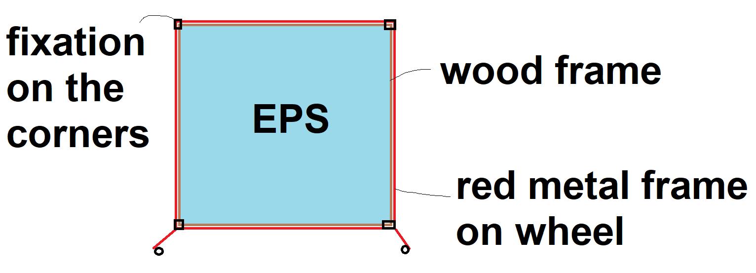
The sample wall is a light wall made by 2 layers of different materials, the first layer is EPS insulation board with 100 mm thickness, another layer is made by OSB board, the thickness of OSB board is only 12 mm. Those 2 layers are fixed with steel plate and screws on a huge metal frame, there is also a layer of wood frame between the metal frame and EPS OSB board. The fixations are separate in the corner of the frame, there are also some in the middle for fixing the EPS board. There are 2 group of wheels under the metal frame, so it is easy to move around.
Figure 1 sketch of the sample wall
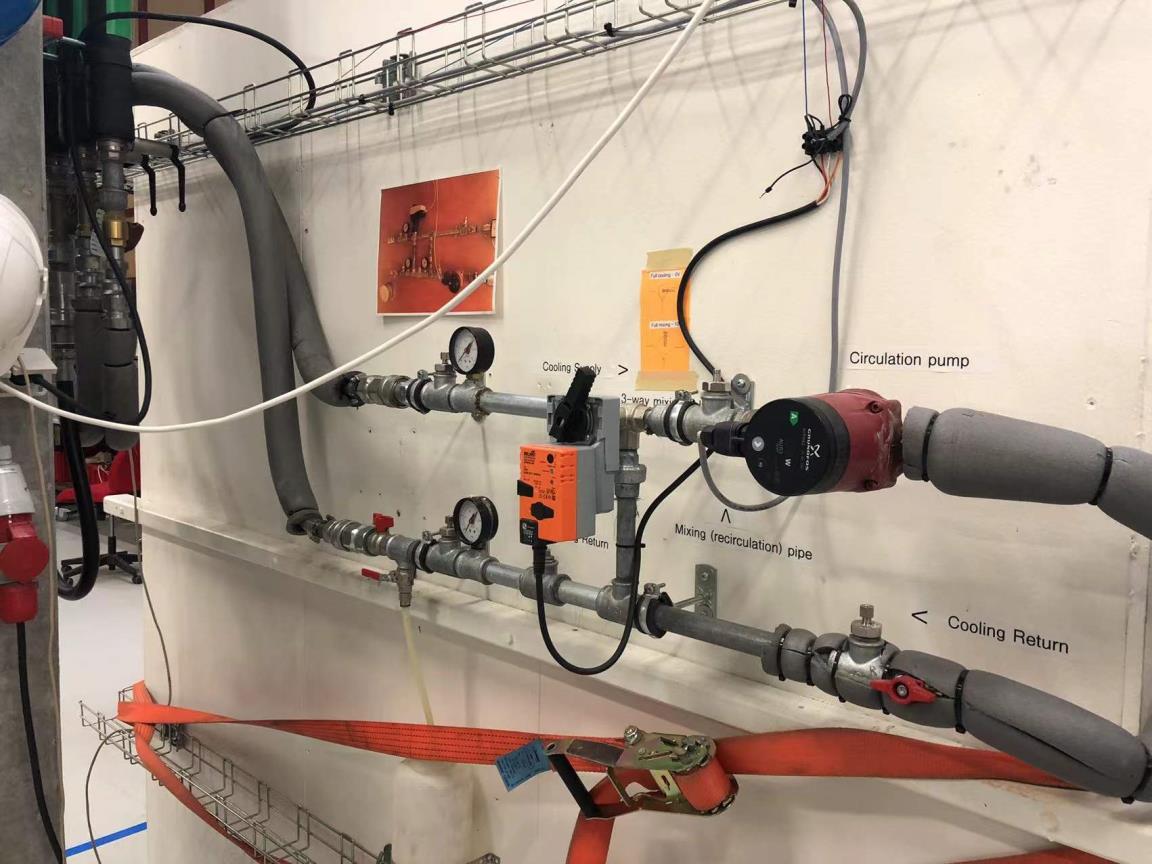
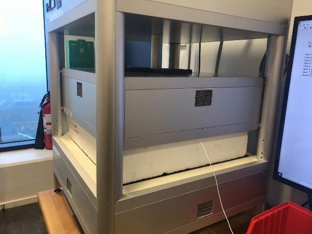
The guarded hot box used in the experiment has a size with 2.7 m*2 m, height is approximately 2.7 m. The inside of hot box is divided into 2 zones, Zone 1 and Zone 3. Zone 2 is used to set for the metering box, but in this experiment it is not used. Zone 1 is set as hot side, it has a cooling system and a heating system module, the cooling did not connect with the supply circle so the cooling pump cannot work properly, and the cooling fan can only create heat but not decrease the temperature in zone 1. The Zone 3 has both workable heating system and heating system, it will be used as the low temperature zone in the subsequent tests with different methods. The cooling supply and return pipe are fixed next to the hot box, due to the cooling supply tunnel, it can provide the cooling system decreasing the Zone 3 temperature to around 12 ℃ 13 ℃, based on that, the temperature in the Zone 3 is usually set as 15 ℃. The
cooling supply water will be going into the Zone 3 and cooling the temperature through a cooler.
Figure 2 cooling pipes for the hot box
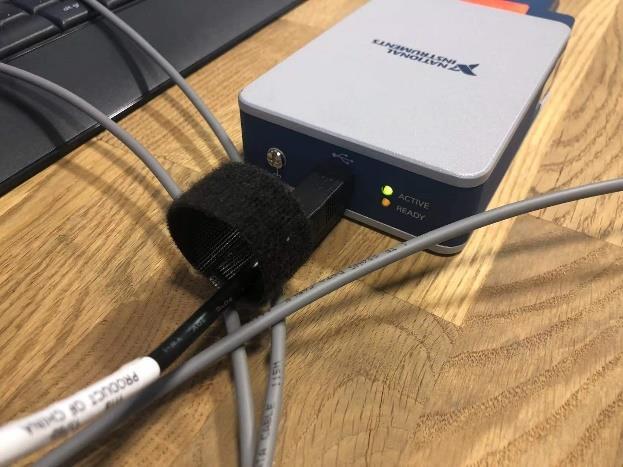
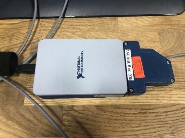
Nearly all the heating, cooling systems and temperature sensors, heat flux sensor and other stuff are connected to a control cabinet on the hot box, it is located on the external surface of the Zone 1. The temperature sensor PT100s and heat flux sensor will be connected with the cDAQ placed in the control cabinet, the cDAQ can receive the data from 8 modules and transport them to the computer through a USB line. There are also other switches and modules to control the power consumption, controlling relays and other functions.
The data transported to computer will be dealing with the Virtual Instrument (VI). VI is created from the LabView which is useful program and can be used to read and control the physical components in the experiment. After coding the relative computer language, it can control the temperature settings in the hot box and create a file to log the data during the test.
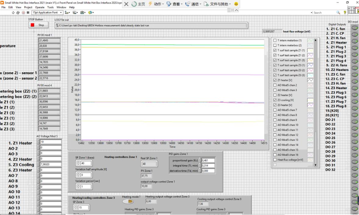
The VI interface include 2 different parts, the one in the front page has several blocks to show different needed information. For example from the Figure 4 interface of the VI, the top side is place showing the position of the recorded data file and the stop button to stop the test. In the middle area, the big screen shows the temperature, heat flux, power output values from the sensors, the parameters showed in the screen can be changed by choosing the name of parameter in the right side block. In the rightmost side, a long block with many buttons can open or shut the function in the hot box, if the cooling fan in the Zone 1 need to be shut down, then only thing need to do is to click the circle button with green mark based on the sequence of the names. On the left side of top part of button’s name, there is a small display box showing the heat flux real time data. The part on the left side of the displaying screen has also the similar function showing the real time data for temperature sensors and voltage output. The bottom side is the area to control the settings for Zone 1 and Zone 3. As the name showing on the setting box, they can be used to set the Zone air temperature, the variation half amplitude and the variation period for the dynamic test. The real SP can show the set temperature in the real time during dynamic test. The PV Zone shows the real time temperature in the Zone, output voltage shows the power output from the heating/cooling system. There is also a PID control panel for set PID value to control the heating and cooling system, those values are tuned by the group so the whole system can reach a steady state environment faster and more stable.
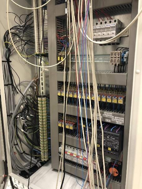 Figure 3 the control cabinet of hot box
Figure 4 interface of the VI
The back page of VI consists by the visual programming code, they have many loops to run the program based on the user requirements and settings. The data from the hot box will be treated here and showing in the front page. The command in the front page like temperature setting will also be handled here and controlled.
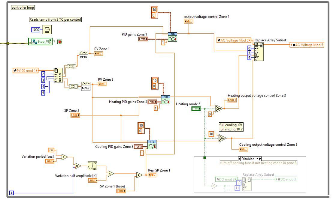
Figure 5 a loop in the back page
3.Literature review
3.1 Steady state methods to calculate the heat flow in building elements
Heat flow meter (HFM)
The first measurement method used in this project is the HFM method as described in DS ISO 9869. In this method thin temperature sensors are placed on the surface of the element and arranged in a way so that the electrical signal can pass through the element and be translated into heat flow. In order to get the most precise results, the HFM should have low thermal resistance and high sensitivity. Additionally, ambient temperature sensors should be considered according to the environmental conditions. Those may include air temperature sensors which are to be shielded against solar radiation or draughts.
The mounting location of the HFMs shall be chosen according to the test and might be investigated beforehand by the thermography imaging. The general rule is that the sensors should be placed in a way which is representative for the whole element and places of possible error such as cold bridges shall be avoided.
The test should be performed for at least 72 hours after the temperature around the HFM has stabilised. There are two available methods for the data treatment: the average method, which is used for simpler steady state conditions, or the dynamic method which is more complicated but allows to shorten the time of the investigation (ISO 9869, 2014)
The test should be performed for at least 72 hours after the temperature around the HFM has stabilised. There are two available methods for the data treatment: the average method, which is used for simpler steady state conditions, or the dynamic method which is more complicated but allows to shorten the time of the investigation (ISO 9869, 2014)
IR thermography
This method has become a popular way of investigating surface temperatures. It is non invasive and can be employed for various investigations of the heat loss through a building element. It is especially useful since it shows surface temperature distributions and can therefore precisely detect spots having higher losses, which can easily detect thermal bridges, cracks or damages of the insulation.
IR can be used together with other methods of investigation. (Mergim Gaši, 2019) suggested in an experiment from 2019 a potential for IR for in situ conditions. They concluded that IR combined with the dynamic method might ensure the approximation of the U value with a higher accuracy than standard methods. Another report by (Fokaides & Kalogirou, 2011) has found the important advantages of the IR
method to be short duration of the measurement procedure and its accuracy, claiming the ‘percentage absolute deviation between the notional and the measured U Values for IR thermography […] in the range of 10 20%.’ The authors believe moreover that another aspect speaking in favour of IR thermography is that the method also considers the radiation effect.
3.2
Dynamic methods to calculate the U-value in building
elements
DS-ISO 9869 Dynamic analysis method
This method, described in DS ISO 9869, can be used to get the steady state properties of a given building element under temperature and heat flow variations. This method presents the building element by its thermal conductance Λ and time constants τ. An identification technique is then applied to find the unknown parameters with a set of linear equations. ���� =Λ(������ ������)+��1������ ��2������ +∑���� �� ( ∑ ������
�� 1 ��=�� �� (1 ����)����(�� ��) +∑���� �� ∑ ������
�� 1 ��=�� �� (1 ����)����(�� ��)
In the formula, TIi and TEi are the indoor and outdoor ambient temperature recorded at time ti. ������ and ������ are the time derivative of the indoor and outdoor temperature, they can be calculated by the difference between 2 recorded value dived by the time step. There are 4 parameters K1, K2, Pn and Qn with no specific meaning in the formula as the variables, they depend on the time constant. The time constant also is related to another parameter ���� which is the exponential functions of the time constant. The time constant is the best estimate of vector �� ⃗ The constant is normally between 1 3, when the m time constants are assumed, the showed formula will have 2m+3 unknow parameter to solve. By using enough data to repeat the formula enough times, an overdetermined system of linear equations can be created. �� ⃗ =(��)�� ⃗ �� ⃗ is the vector related the heat flow data, (X) is the rectangular matrix with the M lines and 2m+3 columns. �� ⃗ is the vector contains 2m+3 components (the unknown parameters) The set of equations can estimate the vector �� ⃗ to have �� ⃗ ∗ , the value
from �� ⃗ ∗ can also estimate the heat flow �� ⃗ ∗ . �� ⃗∗=[(X)′(��)] 1(��)′�� ⃗
In the study from (Gaspar, et al., 2016), compare with the HFM, the dynamic method has only +/ 1% difference with reference value, in addition, the dynamic method can significantly increase the fit with reference value even when the measurement condition is not optimal. However, there is no open source tool was available to the public, it was decided to not spend additional time solving those equations in a program.
Excitation Pulse Method (EPM)
To reduce the monitoring time of the heat flux, a rapid transient in situ measurement technique is introduced, called EPM. In this experimental method, based on the Response Factors theory, a triangular surface temperature pulse is applied to one side of a wall and the temperatures on both surfaces are measured to see how much heat has passed through. This dynamic method introduced by (Arash, 2020) allows the measurement to take much less time. The in situ experiment gave the results in only 1.5 hours with the instrumental error of 6%.
4. Experiment
4.1 Hot plate
The (ISO 7345, 2018) determinates the thermal transmittance of a wall or similar structure as the rate of the transferred energy through a certain amount area of building envelope with the different temperature between both sides under steady state conditions. In the (ISO 6946, 2017) described the theoretical U value calculation by using the materials property and thickness. �� = 1 ������������
Where:
U thermal transmittance of object W/m2K
Rtotal the total thermal resistance of object m2K/W
The Rtotal is the sum of thermal resistance of all the layers in the object, the single layer in the object can be calculated according to: �� = �� ��
Where: R the layer of material’s thermal resistance m2K/W d thickness of the layer mm λthe thermal conductivity of the used material W/Mk
In the real building structure of other similar object, the effects from the air gaps or internal/external surface resistance should also be included as part of the U value calculation. But due to limitation of this experiment, they will be assumed not included
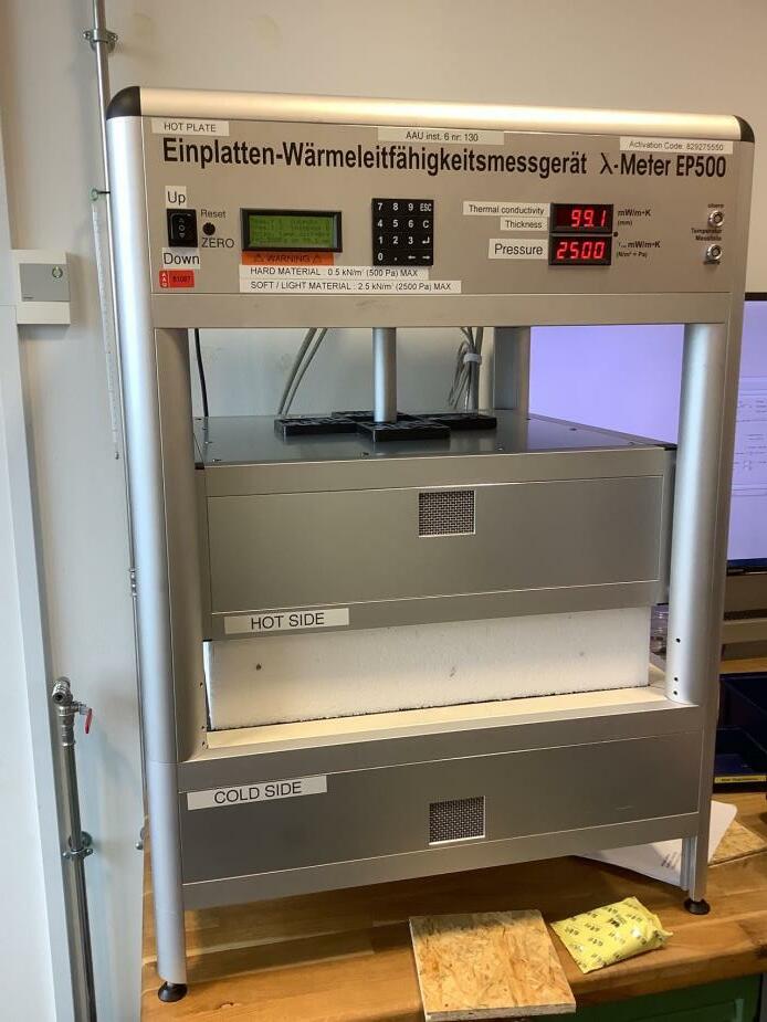
The hot plate machine is a widely used for determining the material’s thermal conductivity. It mainly used the state of the art steady state method, most of the materials are able to find out thermal conductivity by using hot plate. The sample will be placed between 2 sides of hot plate, the hot side and cold side of hot plate will both keep a steady-state temperature boundary condition, then a relatively stable temperature difference and heat flux will be created, at the same time, the direction and speed of temperature changes will also be controlled (Johra, 2019)
Figure 6 the hot plate used in the experiment
There are several parameters monitored for the measurement: the sample surface temperatures on hot side and cold side, the heat flux through the sample, surface area and thickness of the sample. After confirming those parameters, the thermal
conductivity of the sample can be calculated by using the Fourier’s law of heat conduction formula deformation (Johra, 2019)
�� ⃗ = k▽ θ = k ∆�� ∆�� �� =�� ∆�� (��ℎ���� ����������)∗��
Where:
�� ⃗ the local heat flux density, W/m2 k the material’s conductivity, W/mK ▽θ the temperature gradient, K/m
△T the temperature different from both sides, K △x the sample thickness, m
λ thermal conductivity of the material test sample, W/mK
Q heat flux at the center of the test sample, W
Thot temperature of the hot surface of the test sample, K
Tcold temperature of the cold surface of the test sample, K
A section area of the field of measurement at the centre of the test sample, m2
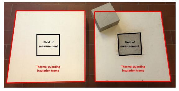
Both insulation materials and non insulating materials can be used in hot plate, for insulation materials, the size is normally 50 cm * 50 cm, the size requirement is smaller for non insulating materials like the OSB board used in the experiment. The surface size is 15cm*15cm, thickness should be from 1 cm to 12 cm. For those non insulating materials, an insulated surrounding is needed to secure the thermal equilibrium with its surroundings The hot plate EP500 type can measure the thermal conductivity range from 0.005 W/mK to 2 W/mK at the temperature from 10 ℃ to 40 ℃(average temperature between the hot plate and the cold plate). The temperature difference between the hot side and cold side ranging from 5K to 15K. When doing the test, there should be a vertical pressure to make sure the thermal contact is enough, the pressure from 0.05 KN/m2 to 2.5 KN/m2 can be set on the sample. The measurement reproducibility error for EP500 is better than 1%, for after short time repetition measurement the error is generally below 0.5%, the test long time after last test is normally within +/ 1%.
Figure 7 Location of the field of measurement, soft insulating materials (left), hard non insulating materials + guarding insulation frame (Johra, 2019)
In order to have a more accurate reference result, 2 test through the hot plate is made. In the first time, 2 different materials made for sample wall are tested separately. When both materials’ thermal conductivity is known, the U value can be calculated based on the method in (ISO 6946, 2017). In the second time, the EPS board was cut to 15 cm * 15 cm size, the thickness is 10 cm as same as the sample wall EPS layer thickness. Both material sample was put together into the hot plate to simulate the real situation in the hot box. Based on the result after the hot plate test, the U value calculation are both close 0.38 W/m2K. The detail hot plate test process and results can be seen in Appendix A hot plate measurement.
4.2
HFM average method
4.2.1 Theory
According to (ISO 8990, 1994), when the amount of heat energy through the warm side to the cold side is known, if there is no other disturbance around the object only the mentioned heat flow effects the object, the U value can be calculated based on the formula:
U= Φ A(���� ����)
Where: U Thermal transmittance, W/m2K
Φ Heat flow rate through the specimen, W A Area perpendicular to heat flow, m2
Ti Internal temperature, K
Te External temperature, K
The (ISO 9869, 2014) states the heat flow meter average method by using the electrical signal from heat flow meter and the known temperature difference. The average method is assumed there is a steady state heat flow through the building envelope, the building envelope has the thermal resistance R can be calculated as the ratio of the measured mean temperature difference between the warm side Ti and cold side Te and the mean recorded heat flow Q. The calculation formula is showing below:
Where:
R thermal resistance, m2K/W
U thermal transmittance, W/m2
Ti internal temperature, K Te external temperature, K Q heat flux per unit area, W/m2
The devices used in the measurement also have requirements. The temperature sensors used in the test should have an accuracy within +/ 2%, if the temperature difference is calculated by subtracting 2 temperatures, the sensors shall have a better accuracy with +/ 0.1 K. The temperature sensors’ calibration needs to perform with several temperature in the relevant range. The thermometer used as reference temperature must have better accuracy than 0.1 K. Normally the data from HFM and temperature sensor should be recorded uninterrupted for at least 72h (3 days) if the temperature near the HFM is stable, if not then the duration should be extended to over 7 days. But there are also some parameters can affect the maximum time step between 2 measurements and the minimum test duration: the nature of element, heavy material has the different minimum test time period with the light material; the indoor and outdoor temperature; and the method used in the data treatment. In order to minimize errors in the test, measurements are better to conduct when the temperature difference is over 10 ℃ (Desogus, et al., 2010). The R value deviation should not exceed +/ 5% between the end and 24 hours before to end the test. However, most of requirements are against the real conditions in site, the surrounding environment conditions created by the hot box can avoid some unnecessary restrictions.
4.2.2 Uncertainty calculation
Not only in experiments, but even in life, all measurement results will carry a certain
�� = 1 �� = ∑ (������ ������) �� ��=1 ∑ ���� �� ��=1
degree of uncertainty. In this experiment, the uncertainty calculation will be used as a reference for evaluating whether the method has advantages. Uncertainty calculations will be divided into two types: theoretical uncertainty and measurement uncertainty. Those uncertainty values will both be used and compared with each other for having a more accurate experiment result. When the measurement uncertainty is way bigger than the theoretical value it means there is problem existed in the experiment. The theoretical uncertainty will be calculated based on the data provided by the equipment manufacturer. In addition, when the value marked on the data is assumed to be 2σ, for example, the PT100 data shows that the uncertainty of the result is +/ 0.1K, 1σ used in the calculation will be +/ 0.05K. When a group of data is being analysed, every single data is normally not same with others, under this condition, the data’s degree of dispersion is approximately normal distribution. If the assumption is correct, then around 68% of the values will located within 1σ from the average. 2σ will have a bigger range with 95%, 3σ means there will be 1% value is out of the range (A Francois et al, 2019).
The calculation of theoretical uncertainty is according to ( Harvard University, 2007)
When there is addition or subtraction in the formula: Q= a + b +··· +c (x + y +··· +z) Then δQ= √δa2 +δb2 +···+δc2 +δx2 +δy2 +···+δz2
When there is addition or subtraction in the formula: �� = ���� c xy···z Then δQ �� = √(δa �� )2 +( δb ��)2 +···+( δc �� )2 +( δx �� )2 +(δy �� )2 +···+( δz �� )2
Where: δ the uncertainty of the parameter (1σ)
Another measurement uncertainty is using standard deviation. The definition of standard deviation is the degree of dispersion between individuals in the group. It can be calculated by using the formula (University of Iowa, 2017): ���� = √∑ (���� ��)2 �� ��=1 ��
Where: SN the standard deviation value N number of samples Xi the value in the group of data x the average value of entire group
4.2.3 Experiment setting and device calibration
The common devices used in this test are:
Instrument Brand and type Measuring range Error Number of devices
Fluxmeter gSKIN XI26 50 ℃ to 150℃ +/ 3% 1
Temperature sensor PT100 75 ℃ to 250℃ +/ 0.1℃ 10
Table 1 devices table
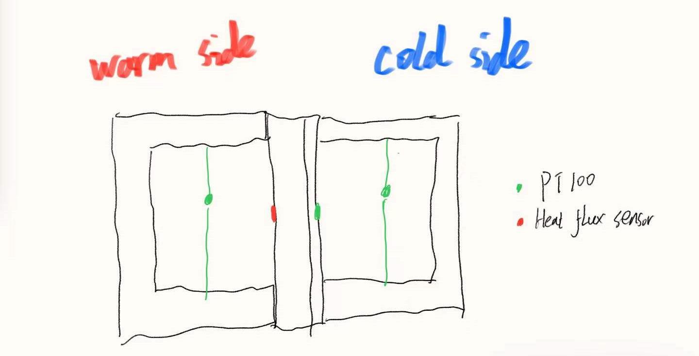
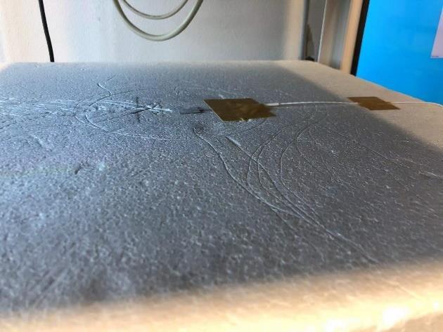
The sample wall will be placed between hot box, EPS board side will face the warm side, the OSB board face the cold side. The heat flux sensor will be placed in warm zone first, taped in the middle area. Each zone has 2 PT100s hanging in the air by the strings between the heating/cooling device to measure the ambient temperature, 3 PT100s on the wall measure the surface temperature.
Figure 8 cross section of hot box in the test
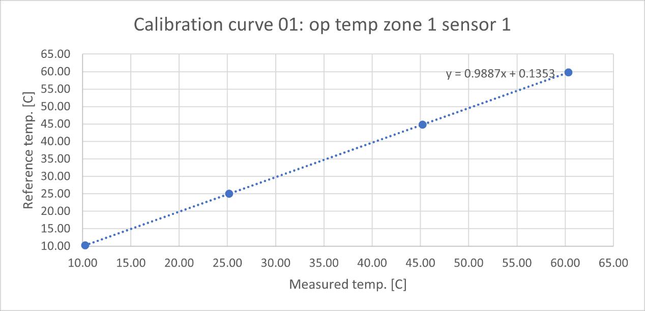
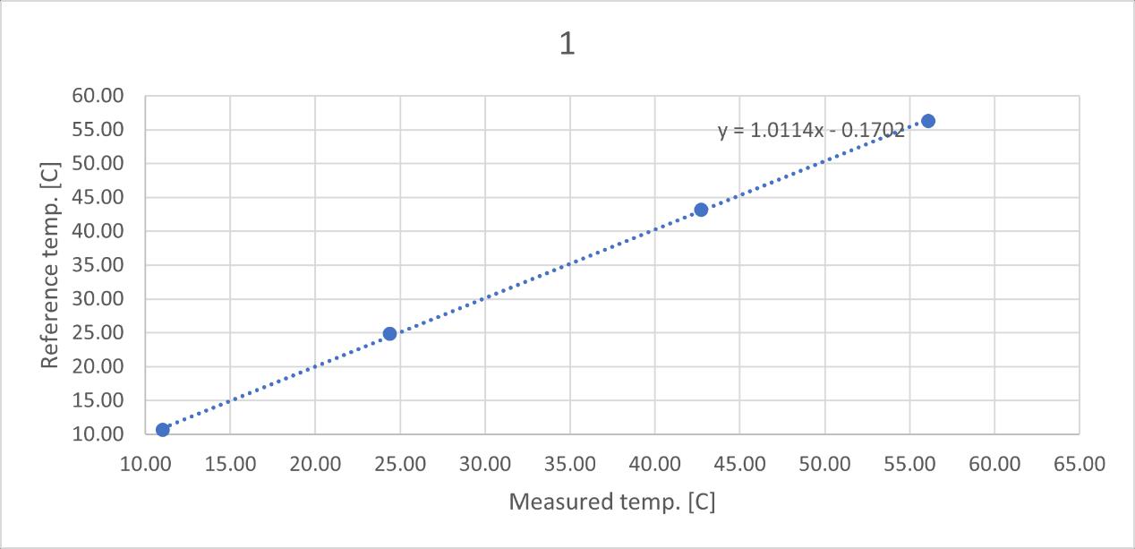
PT100s are calibrated by the F200 Precision Thermometer and Isocal 6, all the PT100s will be placed in the Isocal-6 with the F200 thermometer. Isocal-6 will heat/cool the temperature to the set point, then both PT100s and F200 will give a certain value, based on the reference value from F200, the PT100 can be calibrated to have the real temperature value. 4 temperature set points 10℃, 25℃ ,45℃ ,60℃ are chosen from 10℃ to 60℃ (the experiment temperature range). The detail calibration process can be seen in the Appendix B PT100s calibration
Figure 9 PT100 calibration example
The heat flux sensor is assumed calibrated in the manufacturer company, and since the heat flux sensor will only give the voltage it sense, for having the data with heat flux, there are still require some calculation (Green teg, 2018) �� = �� ��
Where: ϕ heat flux in W/m2 U sensor output voltage in μv S the sensor temperature corrected sensitivity in μv/(W/m2)
4.2.4 Data analysis
Test 1 3
The first method used for simulating U value onsite measurement is the average method. There are 3 test in the beginning have no protection solution for the heat flux sensor and those tests are also more like a test running(the third test period has only 1.5 days, nearly 36h which is way smaller than the 3 days labelled in the (ISO 9869, 2014) but since the sample is thin and made with 2 light materials, the result is still assumed qualified.
Among the first group of tests, except 3rd test set 40℃ in the warm side, the 1st and 2nd tests are set the warm side to 50℃, the cold side are all the same for 15℃. For calculating the U value of the sample wall, only data with +/ 1K is counted as valid data, other parts will be not considered.
Figure 10 the chosen data area
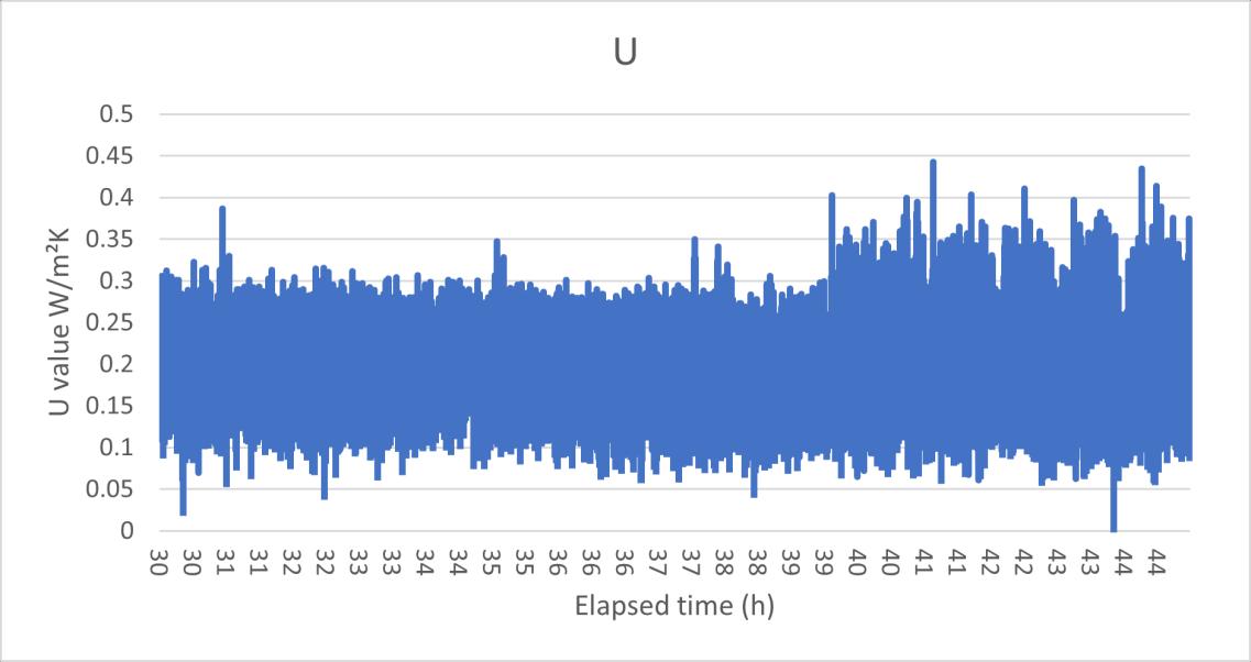
In the first time, the U value result is oscillating from even near 0 to over 0.4 W/m²K, this huge fluctuation is due to the unstable heat flux reading. In the Figure 11 the U value data test 1 and Figure 12 the heat flux data HFM test 1 can be seen that the U value had the same change rhythm with the heat flux, at the same, the surface temperature in the both sides maintained a relatively stable reading. Although in the warm side the temperature showed a slight upward trend, this is assumed still it was a steady state environment, and based on the standard deviation calculating, the error rate in the temperature is only 1.6% which is much smaller than the heat flux (21.6%).
Average when air temperature +/ 1K
Standard deviation Standard deviation/ average (1σ)
Standard deviation/ average (3σ)
U 0.184 0.04 21.5% 64.5% Heat flux 5.66 1.22 21.6% 64.8% Surface temperature difference
30.82 0.49 1.6% 4.8%
Table 2 test results summary of HFM test 1
Figure 11 the U value data test 1
Figure 12 the heat flux data HFM test 1
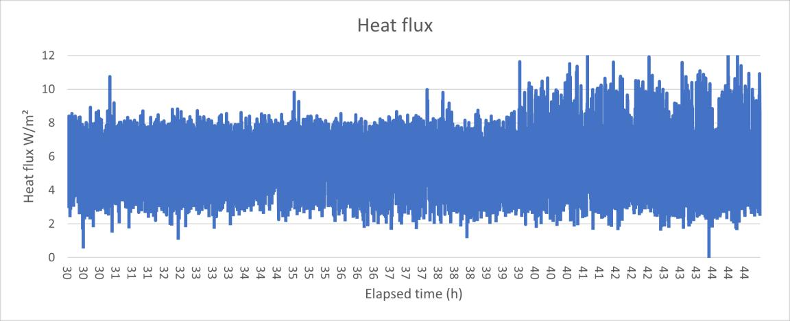

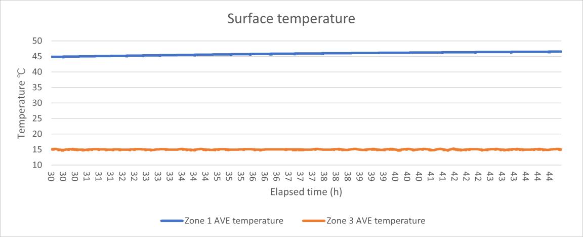
Figure 13 the surface temperature data HFM test 1
In the second test, a problem can affect the U value result was found, the temperature sensor 2 in the warm zone (on the middle of the wall, near the heat flux sensor) showed a very high temperature reading, sometimes the reading was even higher than the 2 sensors for warm zone air temperature.
In order to reduce the impact of high readings, the data from zone 1(warm side) sensor 2 is deprecated, the average surface temperature in the zone 1 will be only calculated by only 2 sensors (zone 1 sensor 1 and zone 1 sensor 3). Although a discovered problem was removed out, according to the calculation results, it was not very helpful.
Average when air temperature +/ 1K
Standard deviation Standard deviation/ average (1σ)
Standard deviation/ average (3σ)
U(before) 0.18 0.04 21.5% 64.5%
Heatflux (before) 5.66 1.22 21.6% 64.8% Surface temperature difference (before)
30.82 0.49 1.6% 4.8%
28.54 0.47 1.6% 4.8%
U (after) 0.20 0.04 21.5% 64.5% Heat flux (after) 5.66 1.22 21.6% 64.8% Surface temperature difference (after)
Table 3 test results summary of HFM test 2
Figure 14 the U value data HFM test 2(after)Figure 15 the heat flux data HFM test 2(after)
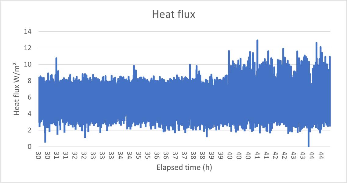
Figure 16 the surface temperature data HFM test 2(after) In the third test, according to the figures below, it can be clearly seen that due to the short running time of the experiment, when the zone air temperature reaches the set temperature, the surface temperature of the sample keeps rising. Therefore, when analysing the third experimental data, the sample interval is divided into two parts, one is taking data when the air temperature reaches the set temperature, and the other is taking data when the sample surface temperature fluctuates regularly.
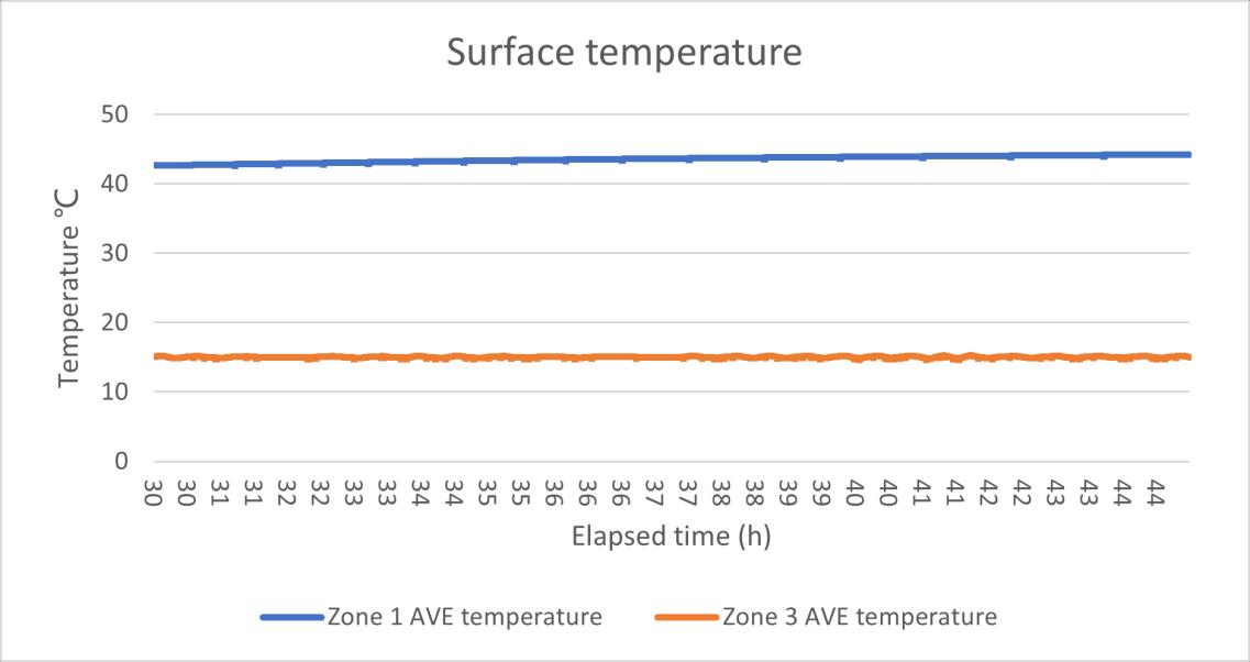
Figure 17 the U value data HFM test 3.1
Figure 18 the heat flux data HFM test 3.1
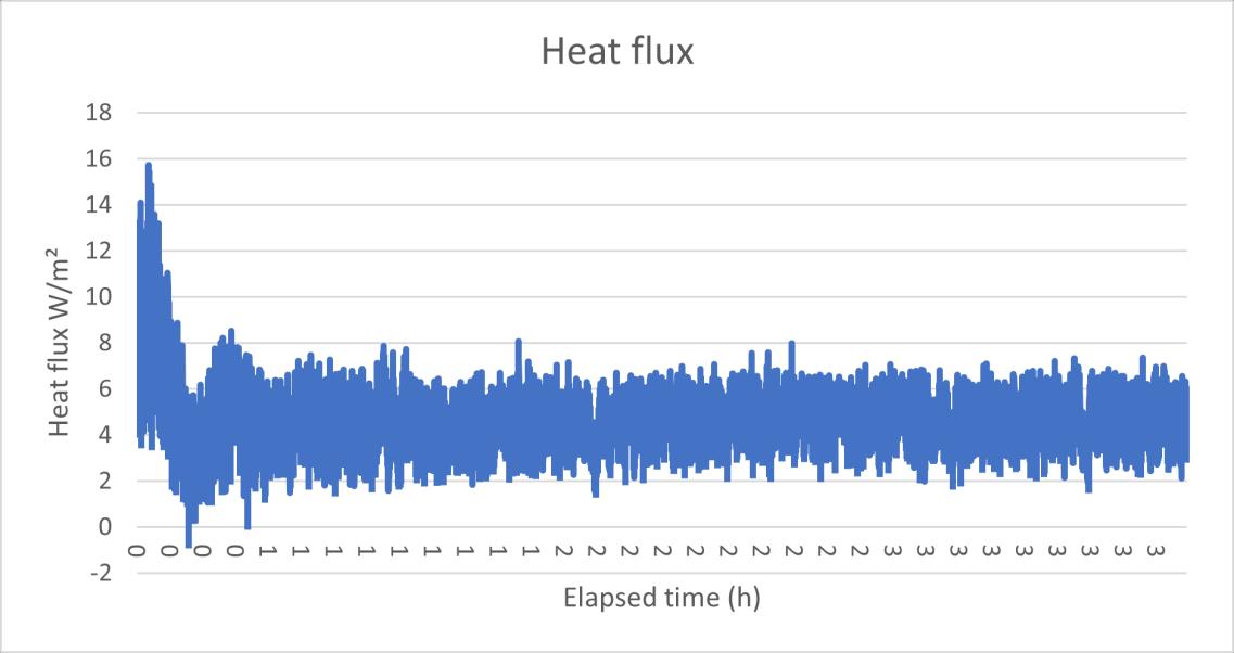
Figure 19 the surface temperature data HFM test 3.1
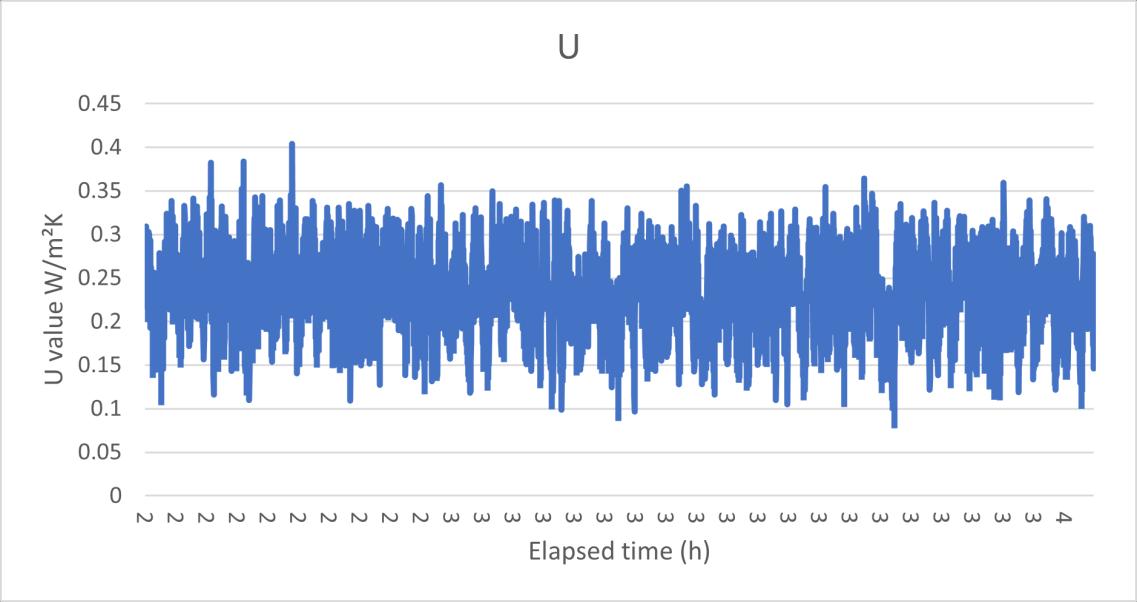
Figure 20 the U value data HFM test 3.2
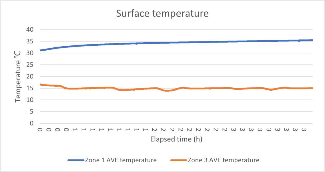
Figure 21 the heat flux data HFM test 3.2
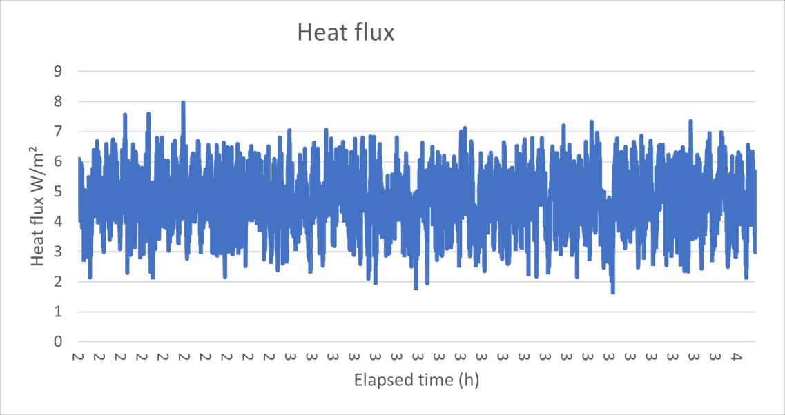
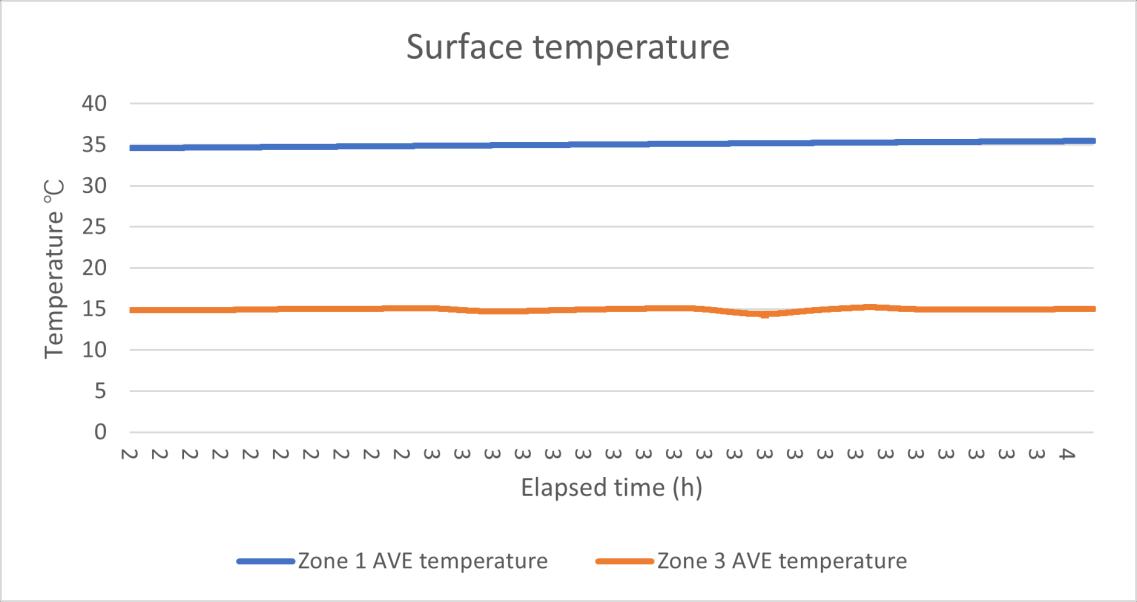
Figure 22 the surface temperature data HFM test 3.2
Average when air temperature +/ 1K
Standard deviation Standard deviation/ average (1σ)
Standard deviation/ average (3σ)
0.25 0.08 33.1% 99.3% Heat flux (3.1) 4.72 1.26 26.6% 79.8%
U(3.1)
Surface temperature difference (3.1)
19.28 1.33 6.9% 20.7%
U (3.2) 0.23 0.04 19.1% 57.4%
Heat flux (3.2) 4.71 0.90 19.1 % 79.8%
Surface temperature difference (3.2)
20.1 0 31 1.5% 4.5%
Table 4 test results summary of HFM test 3
As a small summary, in the above three experiments, although some observed errors were removed to achieve better results as much as possible, the results U value was not very ideal. The U values of the three experiments were all around 0.2 W/m2*K, there is generally an error nearly 50% from the theoretical value. The reason for the huge error may be that the hot box cannot be completely closed. Although a belt tensioner is used to help close the hot box, it is still suspected that there are some small holes existed can affect the experimental results. On the other hand, the heat flux sensor has shown extremely unstable readings in those experiments. This problem may be caused by the heater as the heat supply of the warm zone create a strong draught directly on the heat flux sensor. In the calculation of the average method, U value is calculated by the temperature difference between the cold and warm sides and the thermal energy displayed by the heat flux sensor. As one of the main parameters, extremely variable data will inevitably cause greater errors in the calculation results and cause bad effects.
The fourth test
During the previous tests, the different temperature settings in the warm side seems has effect on the U value calculation, the heat flux standard deviation is also different. The fourth test is mainly to investigate if the different temperature setting or different temperature difference has an influence on U value calculation.
Figure 23 the U value data HFM test 4.40
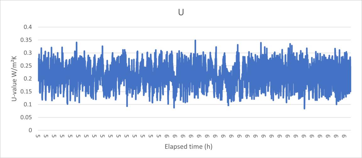
Figure 24 the heat flux data HFM test 4.40
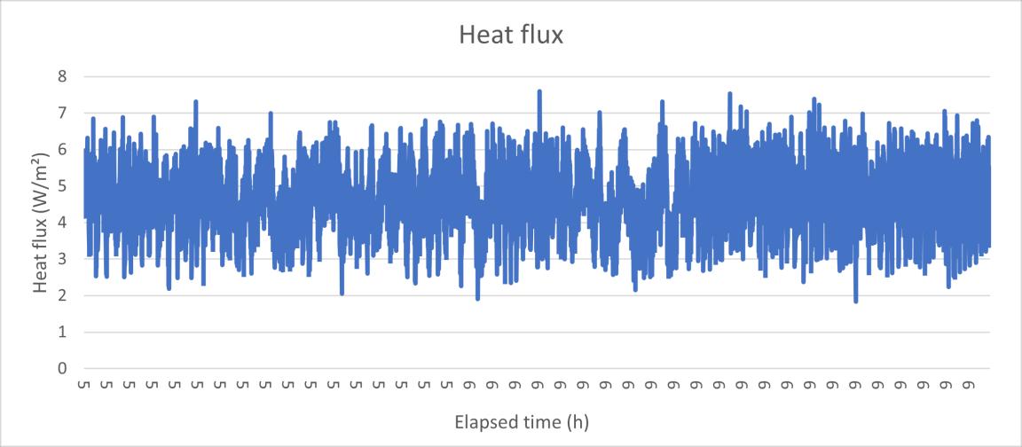
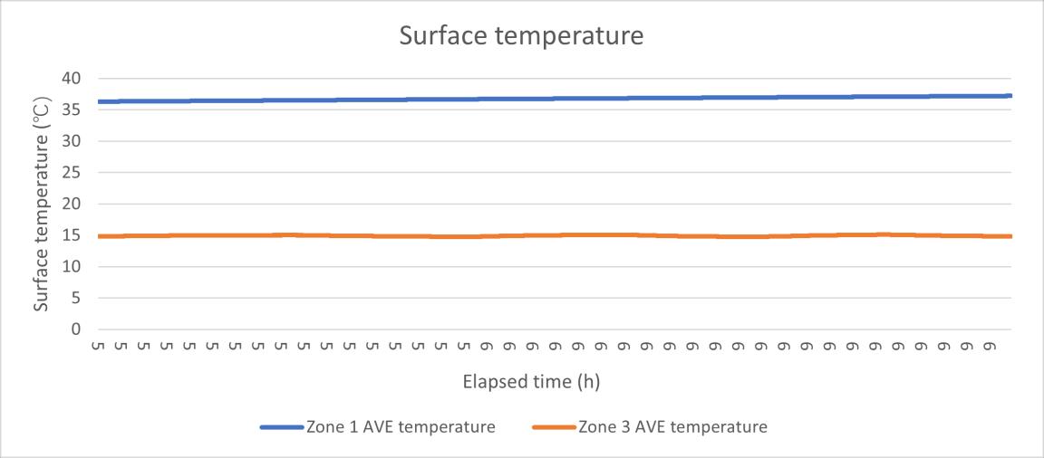
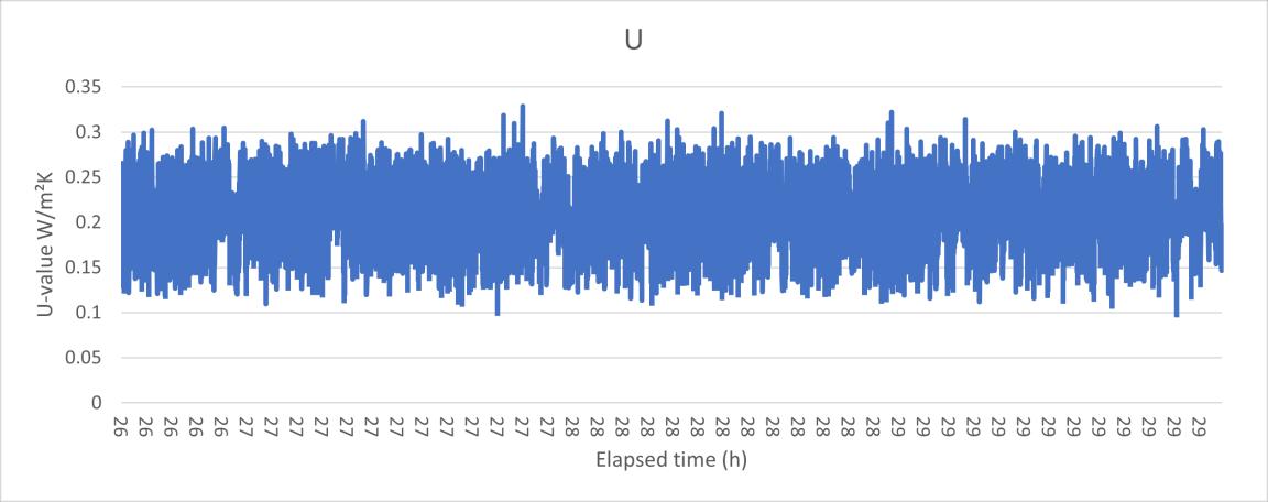
Figure 25 the surface temperature data HFM test 4.40
Figure 26 the U value data HFM test 4.50
Figure 27 the heat flux data HFM test 4.50
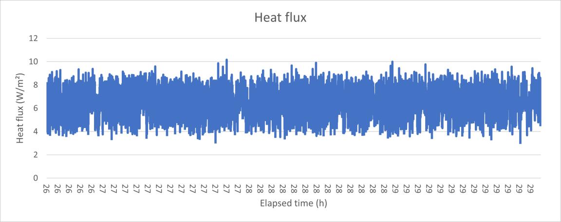
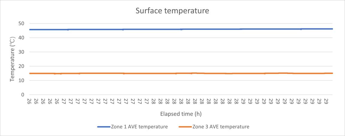
Figure 28 the surface temperature data HFM test 4.50
Average when air temperature +/ 1K
Standard deviation Standard deviation/ average (1σ)
Standard deviation/ average (3σ)
U(4.40) 0.23 0.04 19.1% 57.4% Heat flux (4.40) 4.65 0.89 19.2% 57.6%
Surface temperature difference (4.40)
19.90 0.27 1.4% 4.1%
U (4.50) 0.23 0.03 16.2% 48.7% Heat flux (4.50) 6.52 1.06 16.2 % 48.7%
Surface temperature difference (4.50)
28.6 0 14 0.5% 1.5%
Table 5 test results summary of HFM test 4
Based on the table and figures showing, the temperature setting has no big influence on u value result, the 2 tests have very similar U value, but the heat flux and U value has a little better stability. However, these problems still existed during the experiment, for example, during the experiment, the cooling fan and pump in the warm zone were still running when there is no need to cool down which caused the unnecessary temperature rising. The temperature rise also brings another problem, that is the duration of the experiment. As mentioned in the previous paragraph, the experimental data is considered valid when the air temperature is +/ 1°C. The continuous increasing temperature reduces the time when the temperature is in this temperature range and reduces the number of samples. Due to time constraints, it is impossible to make further investigations about this question in this experiment, but in theory, this experiment should set more groups of temperature differences, there is only one test, and the temperature difference of 10K in this experiment did not bring a significant change.
Test5 7
From the previous data, it is not difficult to see that the varied heat flux is a factor that mainly affects the U value calculation. Therefore, how to protect the heat flux sensor to obtain relatively stable readings has become the main goal of this stage. After discussion, there are several methods used during the test, first method is putting some thermal paste on the heat flux sensor to avoid the directly air jet. Second method is on the basis of method 1 add a hard tape to cover the heat flux sensor.
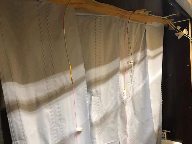
The last method is using some paper fabric between the sample wall and heater, the bottom side of paper fabric use tape stick the paper with the hot box
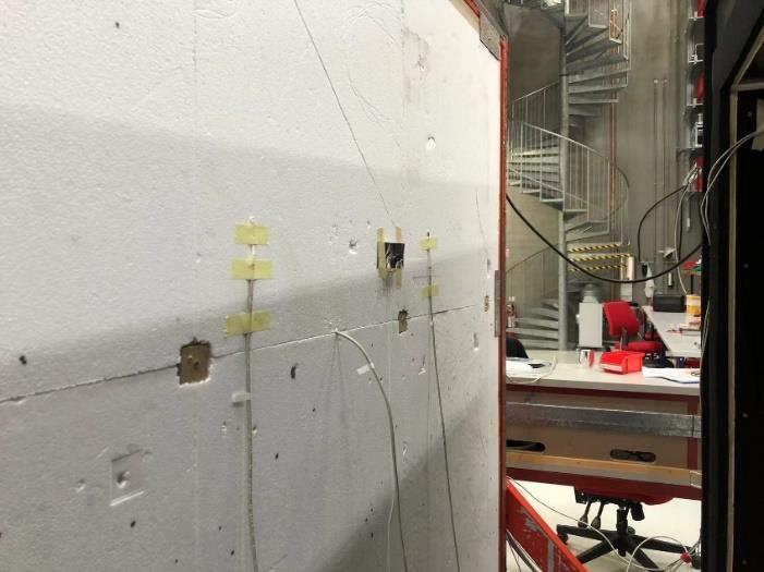 Figure 29 cover on the heat flux sensor
Figure 30 paper fabric cover in the hot box
Average when air temperature +/ 1K
Test 5 thermal paste+ hard cover
Standard deviation Standard deviation/ average (1σ)
Standard deviation/ average (3σ)
U 0.21 0.04 17 2% 51 6% Heat flux 4 31 0.73 17.2% 51.6% Surface temperature difference
19.8 0 27 1.4% 4.2%
Test 6 paper fabric cover warm zone 40
U 0.15 0.04 26.1% 78.4% Heat flux 3.88 1.01 26.1% 78.4% Surface temperature difference
25.1 0.19 0.8% 2.4%
Test 6 paper fabric cover warm zone 50
U 0.21 0.03 14.1% 42.4% Heat flux 7.33 1.04 14.1% 42.4% Surface temperature difference
35.1 0.14 0 4% 1 2%
Table 6 test results summary of HFM test 5 6
Except for test 6 paper fabric cover warm zone 50, the protective methods used in experiments did not improve the situation on the heat flux. In the test 6, the U value and heat flux have very close standard deviation result but since the higher average
heat flux value the error rate is smaller than the result in the test 6 paper fabric cover warm zone 50
In order to answer whether the unstable heat flux reading is caused by the heater airflow, in the next groups of tests, the data will be recorded when air temperature in both zones reach the set point and close the heater fan. Under this situation, the inside of hot box can still keep a shortly relatively steady state. The heat flux is also placed in the cold side to check performance.
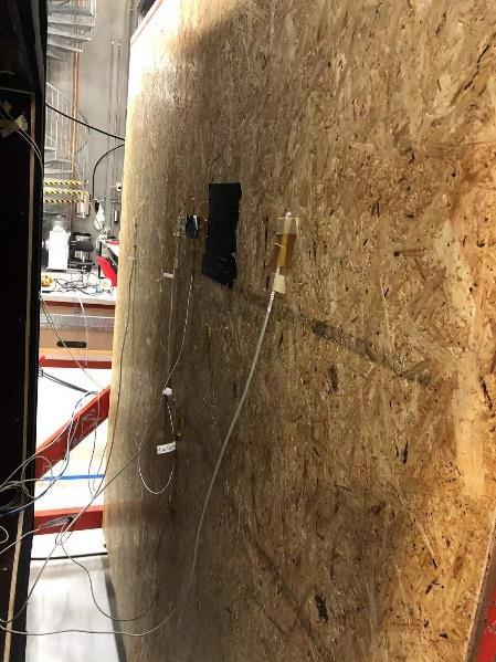
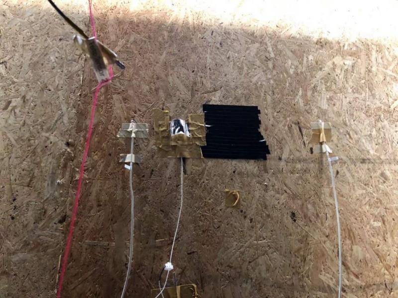
Table 7 heat flux placement in Zone
3
The first problem under this situation is the air temperature in the zone drop very fast after turned off the heating fun and pump. In the previous tests the group assumed it is still steady state when the temperature is +/ 1K, but based on Figure 31 heat flux oscillation after turn off the heating systemshows the heat flux amplitude of wave is very huge. So under this condition, the data will take from a period with more stable part.
Figure 31 heat flux oscillation after turn off the heating system
However, when the heat flux sensor is placed on the cold side, due to the temperature difference, the heat flux reading fluctuates just around zero when it is relatively stable. In the calculation for the test 7, the data will be taken from the beginning time after turning off the cooler.
Average when air temperature +/ 1K
Standard deviation Standard deviation/ average (1σ)
Test 7 heat flux in cold side (closed the cooler)
Standard deviation/ average (3σ)
U 0.073 0.02 31.0% 93.0% Heat flux 1.76 0.55 31.0% 93.0% Surface temperature difference 23.9 0.07 0.3% 0.9%
Test 8 heat flux in warm side (closed the heater)
U 0.086 0.02 28.5% 85.5% Heat flux 2.00 0.57 28.5% 85.5% Surface temperature difference 23.1 0.04 0.2% 0.6%
Table 8 test results summary of HFM test 7 8
According to the Table 8 test results summary of HFM test 7 8, it can be seen that the heat flux still keeps changing violently after turned off the heater/cooler, which means the air jet from heating/cooling system is not the only one parameter effects the experiment. The data for all the HFM tests are in the Appendix E HFM tests results
Figure 32 compare table HFM tests
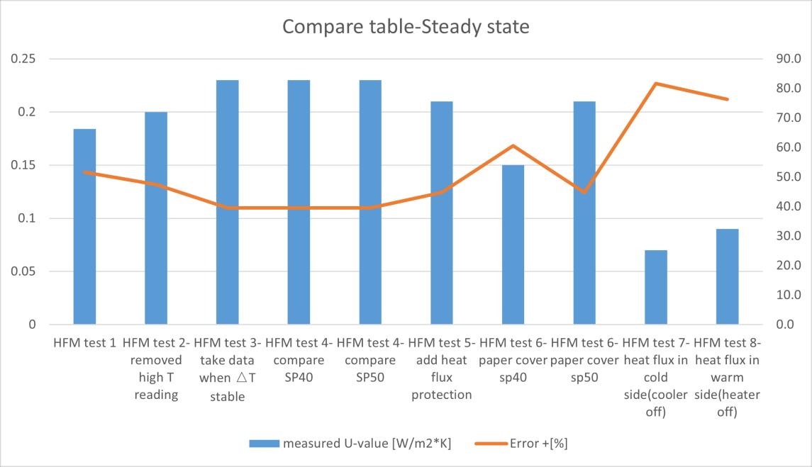
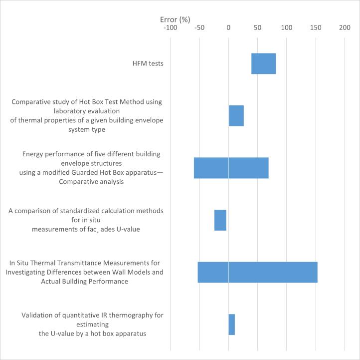
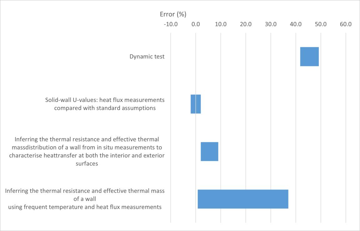
Figure 33 Error rate HFM tests compare with literature
4.3 Laser thermometer
4.3.1 Theory description
One of the most significant differences in infrared technique from other temperature measurement methods is that it is a non invasive method. In addition, IRT is also regarded as a fast solution in a quasi steady state condition, which can generally collect
data on the building envelope in a short period of time. Different with HFM, the IRT will consider both convection and radiation but not only conduction. However, this also makes it extremely vulnerable to climatic conditions, high emissivity pollution and smog. At the same time, it also has higher requirements for data collection and processing, and the cost is generally higher. There are many experiments done according to the methodology proposed by (Fokaides & Kalogirou, 2011) using a thermal camera to calculate the U value of the specimen The theory of IRT method is also similar with the HFM method: �� = εσ(���� 4 �������� 4 )+ℎ��(���� ��������) ������ ��������
Where: U the thermal transmittance, W/m2K Ɛ emissivity of the specimen, σ the Stefan-Boltzmann constant, equal to 5.67*10 8 Tw the temperature of the external surface of the measured specimen, K Tout the out door air temperature, K Tin the in door air temperature, K hc the convective heat transfer coefficient, W/m2K
However, in this experiment, assuming that the convection will not be considered by the experiment, the team chose another experimental method by using the temperature data from the IR thermometer replace the data from PT100s, the heat flux sensor will still record the data during the test, the formula will be as same as the HFM average method: �� = 1 �� = ∑ (��������.�� ��������.��) �� ��=1 ∑ ���� �� ��=1
Where: R thermal resistance, m2K/W U thermal transmittance, W/m2 TiIR warm side surface temperature measured by IR thermomoter, K TeIR cold side surface temperature measured by IR thermomoter, K Q heat flux per unit area, W/m2
4.3.2 Experiment setting and device calibration
The devices used in this test are:
Instrument Brand and type Measuring range Error Remark Fluxmeter gSKIN XI26 50 ℃ to 150℃ +/ 3% Temperature PT100 75 ℃ to +/ 0.1℃
sensor 250℃
Laser thermometer
1
Laser thermometer
2
AMIR 7811 0℃ to 50℃ +/ 1℃
Thermo Control I, Infrarot, Berner
Table 9 IR test devices table
50 ℃ to 550℃ +/ 2℃ Display range: 0.5 ℃
The laser thermometer 2 has no detail information in the manufacturer website, the introduction from an advanced version is assumed as same as the laser thermometer 2. There is also no emissivity setting function in this laser thermometer, so an assumed emissivity 0.95 from the advanced version is used in test.
The 2 laser thermometers are calibrated by using F200 Precision Thermometer and Isocal 6, they are the devices used for calibrating PT100. Because the chamber in the Isocal 6 is made by metal, it has different emissivity to the black body, the electrical tape (black and emissivity is 0.95) is used to cover the top side of Isocal 6 chamber
The F200 Precision Thermometer is not placed in the bottom but close to the black tape, it’s temperature measured will be used as the ref temperature (the set temperature is 10°C, 25°C,45°C and 60°C). When the temperature in the Isocal 6 is stable then quickly opened the cover and measured the temperature on the tape. Once the data are collected, the calibration formula can be calculated. The detail data is showing in the Appendix C IR thermometer calibration
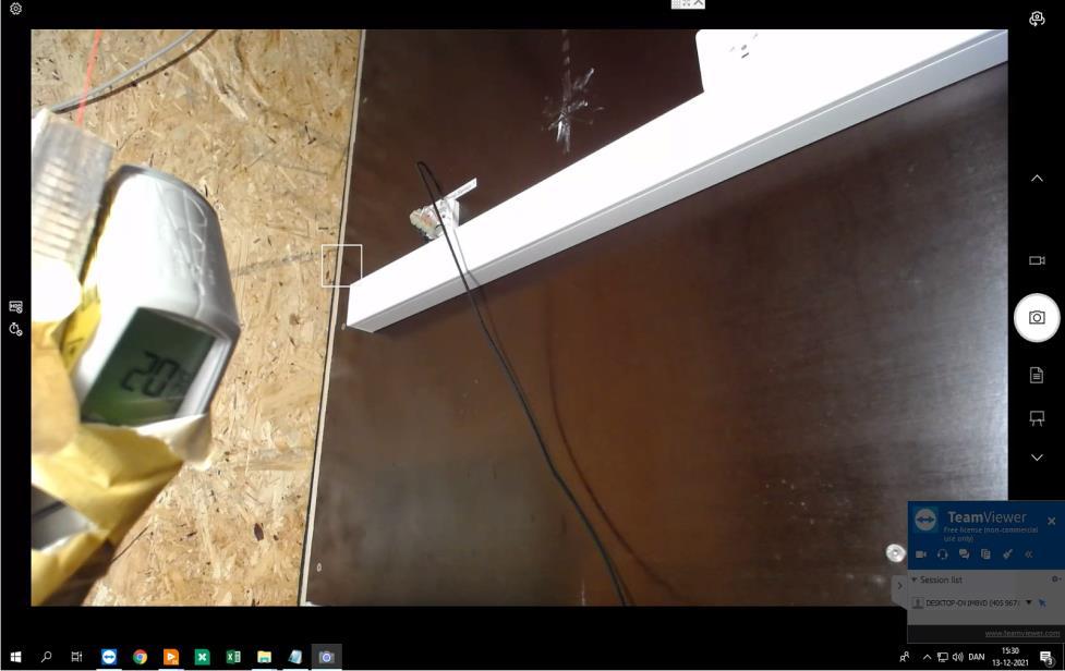 Figure 34 picture during IR test 2
Figure 35 Laser thermometer 1 calibration
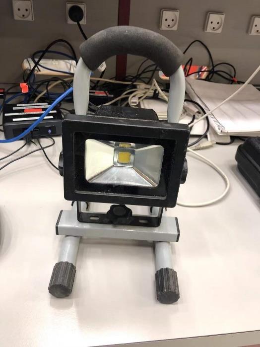
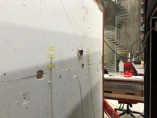
On the sample wall, in the middle area near the heat flux sensor, there are some black electrical tapes with known 0.95 emissivity covered on it. Laser thermometer 1 is put in the warm zone and laser thermometer 2 is in cold zone. The laser is taped with supporting for pointing the target area, each laser thermometer has 1 webcam right behind, a light near by to provide visibility. The lights are also different, the first light is a LED light with less power(10W), another one is an incandescent lamp, it has bigger power than the LED light but also create more heat may affects the test. The incandescent lamp in the first test was in cold zone and transported to warm zone for other tests.
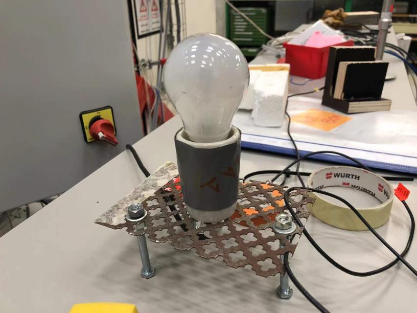 Table 10 different type of light
4.3.3 Data analysis
The data will be analysis like the average method, 2 laser thermometers will record the surface temperature in both sides, time period between 2 measurement point is 10 minutes. The heat flux is the average value in 60 second.
There are 3 measurements, every measurement has 40 minutes totally. The first test is not very accurate since the laser thermometer did not fix tight with the supporting, the focus point did not shoot to the black tape area. The second test and third test are the same running from different time, and zone 1 air temperature was rising because heat from cooling fan in the warm side. Since this method is generally used on site as a fast method and does not have very high temperature requirements like HFM, the experimental data is still considered acceptable.
IR test 1
1 2 3 4 Average
Heat flux 3.48 3.38 2.58 2.01 Surface temperature warm side 38.3 38.5 38.7 38.7 Surface temperature cold side 15.6 16.1 16.1 16.1
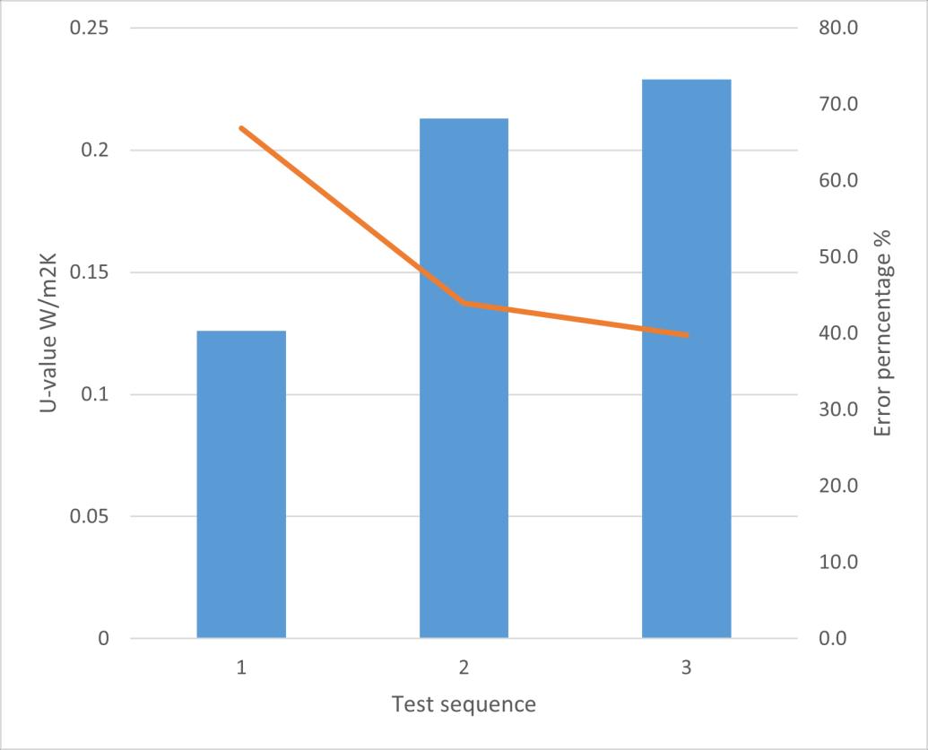
U 0.154 0.151 0.112 0.087 0.126 IR test 2
1 2 3 4 Average
Heat flux 3.67 3.81 3.80 3.35 Surface temperature warm side 36.4 39.7 39.9 40.2
Surface temperature cold side 21.5 21.5 22.0 22.0
U 0.246 0.210 0.213 0.184 0.213 IR test 3
1 2 3 4 Average
Heat flux 4.54 5.07 4.58 4.88 Surface temperature warm side 42.7 42.7 42.9 43.0
4Surface temperature cold side
22.0 22.0 22.0 22.0
U 0.220 0.244 0.219 0.232 0.229
Table 11 test results summary of IR test 1 3
Except the IR test 1 has a lower value than others, the rest of measurement result are close to the U-value calculated by heat flux average method. However, in the temperature in the cold side shows a significant difference between IR test 1 and IR test 2/3. At the same time, in the data from PT100 in the cold zone, it shows the surface temperature in the cold zone is always around 15℃ during the test period.
Figure 36 IR test 2 cold zone surface temperature
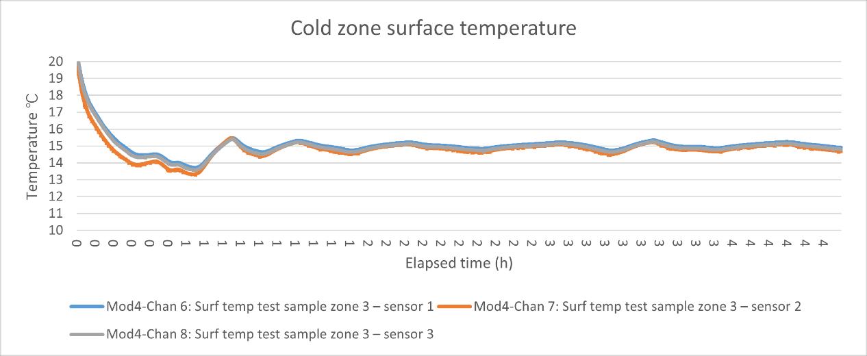
Figure 37 the heat flux data IR test 2
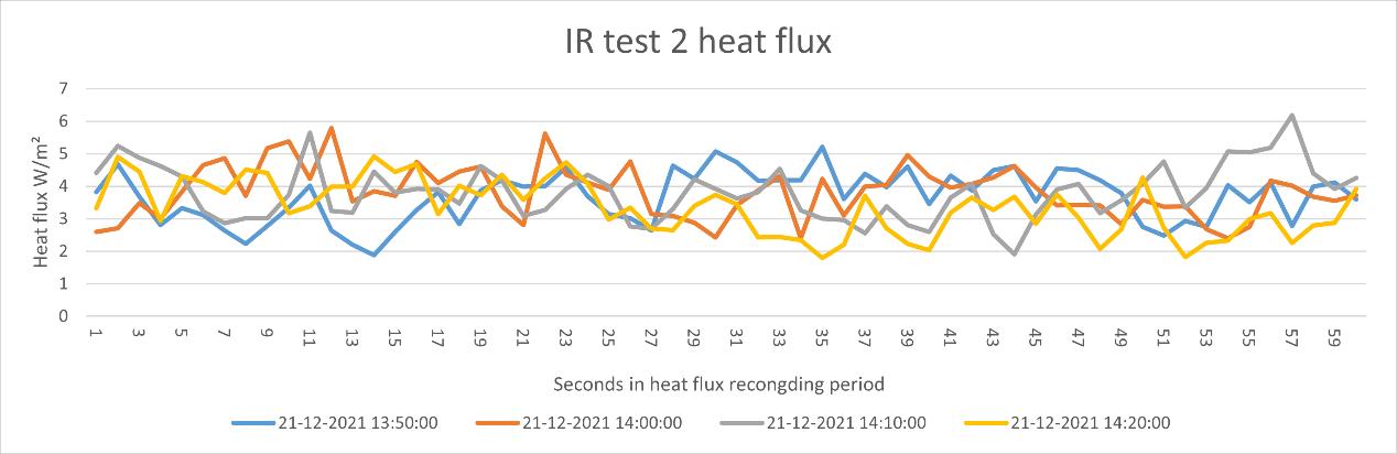
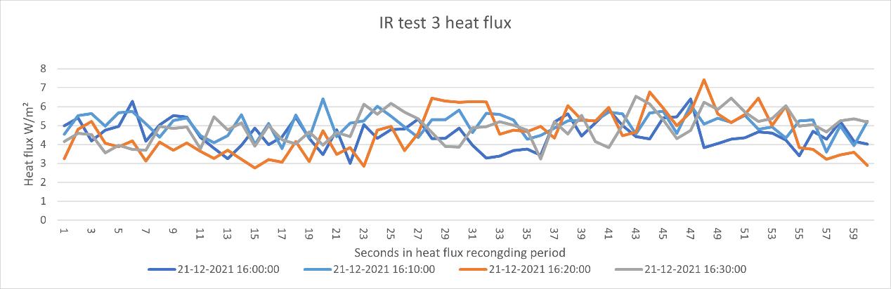
Figure 38 the heat flux data IR test 3
The group also doubted that there is maybe thermal bridge between 2 zones through
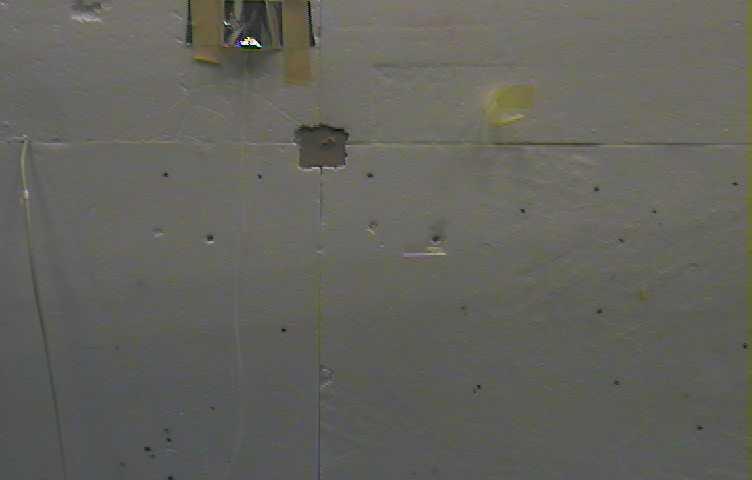
the sample wall, a thermal graph camera is used to look over around the whole wall, based on the infrared photos taken right after one test, there is no huge temperature difference in the sample wall area except the connecting nails. The other photos are put in the Appendix H photos from thermography camera.
Figure 39 thermal Imaging of sample wall right after a test
Due to the limited time and number of people, it is hard to do more tests and investigation. But the plan should be focus on calibrating the heat flux value and verifying the temperature. For example, the 2 laser thermometers can switch to another zone, the recorded value can also be used to compare with the previous test data. The detail data for IR tests is in the Appendix F IR tests results.
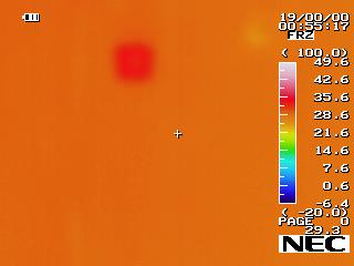 Figure 40 compare table laser thermometer tests
Dynamic
4.4.1 Theory introduction
Lumped thermal mass method
Developed by (Biddulph et al., 2014), a method combined a lumped thermal mess model and a Bayesian based inverse optimization technique to estimate the thermal properties in the situ measurement. Like most of the U value calculation method, the lumped thermal mass method (or called single thermal mass method, 2R1C model) also uses the heat equation as the theory basis Based on the HFM average method the thermal transmittance U is equal to the heat flux divided by the temperature difference between hot and cold side equal to reciprocal of R value. Then if the sample wall is assumed to be 2 parts, each part has a thermal resistance R1 and R2, the total object has a magnitude of thermal mass per unit area C, and the temperature of the thermal mass at the beginning point ���������� 0 The formula during a time step p can be transformed to (Li et al, 2014):
Where: U the thermal transmittance, W/m2K R1,R2 the simulate R value for each part of object, m2K/W ������ �� the assumed constant heat flux entering the object from warm side, W/m2
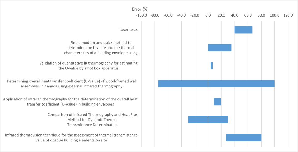
Figure 41 compare table laser tests with literature 4.4
��= 1 ��1 +��2 ������ �� = (������ �� ���������� �� ) ��1
������ �� the temperature on warm side of the object at a time step p, K ���������� �� the temperature on thermal mass at a time step p, K And if the temperature of the thermal mass is known, the temperature of thermal mass at next time step duration(τ) can be calculate based on the heat flow balance forward difference equation: �� ���������� ��+1 ���������� �� �� = ������ ��+1 ���������� ��+1 ��1 + �������� ��+1 ���������� ��+1 ��2 ���������� ��+1 =
������ ��+1 ��1 + �������� ��+1 ��2 +�� ���������� �� �� 1 ��1 + 1 ��2 + �� ��
Where: C assumed thermal mass per unit area, J/m2K ���������� ��+1 the temperature of thermal mass at next time step duration, K τ time step duration, s ������ ��+1 the temperature on warm side of the object at next time step duration, K �������� ��+1 the temperature on cold side of the object at next time step duration, K �������� �� the temperature on cold side of the object at a time step p, K
Once a group of temperature data for warm side and cold side is set, combined with any set of C, R1, R2 and initial thermal mass temperature, the predicted heat flux time series through object can be calculated by repeating the showed formulas. There is also more complicated method by assuming more thermal mass parts in the object for example 3R2C model, with more assumed parameter in the formula it normally can provide more accurate result. Since the limited equipment and time, there will only single thermal mass method in this experiment (Gori, et al., 2016).
For a reference value compare with the best simulate value, the R1 and R2 will used the thermal resistance value from the hot plate value since the temperature sensor to measure the thermal mass temperature will be placed between 2 layers of the sample wall, the reference thermal mass calculation is based on the method from (Biddulph et al., 2014): C���������������� =����������������������,����������������������������������
Where: C the material’s thermal mass per unit area J/m2K ρ the density of material Kg/m3 cp the specific heat capacity of material J/KgK d the thickness of layer made by material m
The thermal mass for the sample wall is made with 2 different materials: EPS and OSB board. The OSB board density is assumed equal to 600Kg/m3 (TRADA, 2014) and specific heat capacity is 1550 J/KgK (Czajkowski, et al., 2016), the thermal mass per unit is calculated to 11160 J/m2K in 0.012 m thickness. The EPS board has assumed density 11 Kg/m3 (Australian Urethane & Styrene, n.d.) and the specific heat capacity is 1210 J/KgK (Engineering ToolBox, 2003) (Material Properties, 2021), so the thermal mass per unit is calculated to 1331 J/m2K in 0.1 m thickness. The total thermal mass for sample wall is the sum of 2 layers which is 12491 J/m2K.
4.4.2 Experiment setting
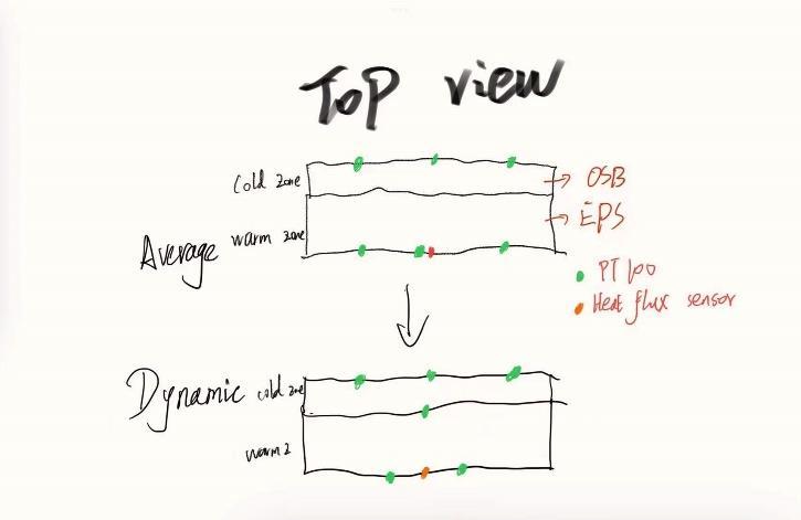
The setting of dynamic test is similar to the average method except 1 PT 100 in the warm side will be put from the surface to the middle of the wall, between the EPS board and OSB board. The other 2 PT100 in the warm zone will be moved and separated to both sides of heat flux sensor, but distance of them will be closer than before.
4.4.3 Data analysis
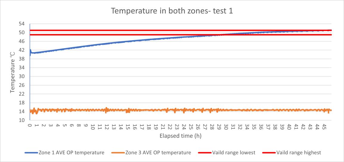
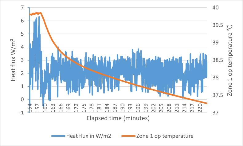
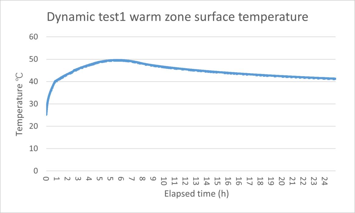
The data is analyzed by CTSM R, warm zone initial temperature is 40℃, a 10 K variation half amplitude is set within 86400s (24 hours).The cold zone set point will be 15℃ as constant. In the experiment, there is a problem that cannot be solved in the short term is no cooling device in the warm zone, so it is difficult to really reduce the temperature of the warm zone to the expected temperature in the dynamic test. Generally the temperature will be decreased to around 42℃ then going up to 50℃ to finish a loop. After the second dynamic test, new variation half amplitude with less time period (43200s) was set for investigation.
Table 12 dynamic test settings and sketchFigure 42 the surface temperature during the dynamic test 1
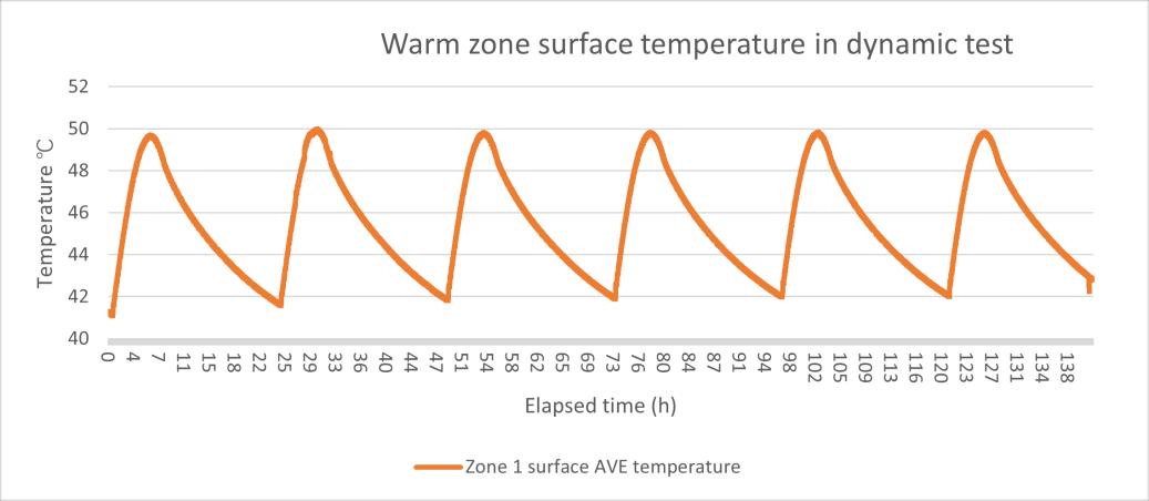
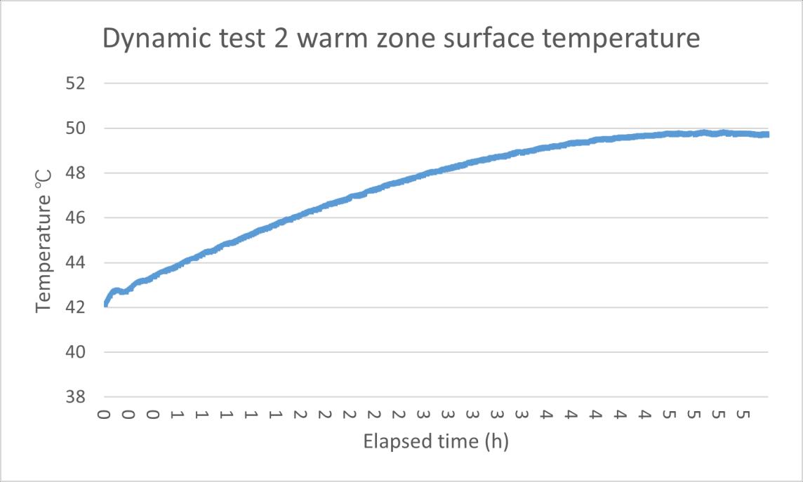
There are 3 dynamic tests used to analysis the U-value. The first one test used data including temperature rising and dropping, test2 and 3 only have the part when temperature rising
Figure 43 surface temperature data for analyzing dynamic test 1
Figure 44 surface temperature data for analyzing dynamic test 2
In the CTSM R, the data will be analyzed by the R code. First the system needs the formulars to create model, so the 2R1C formular will be used in the system. Then the initial point for some parameters are required for simulation, for example the initial temperature in the mass, thermal resistance R1 and R2, the lumped thermal mass per unit area C. The other parameters like Ti and Te will be import from Excel and used for the estimation. All the result will list as a table, it can be present as picture.
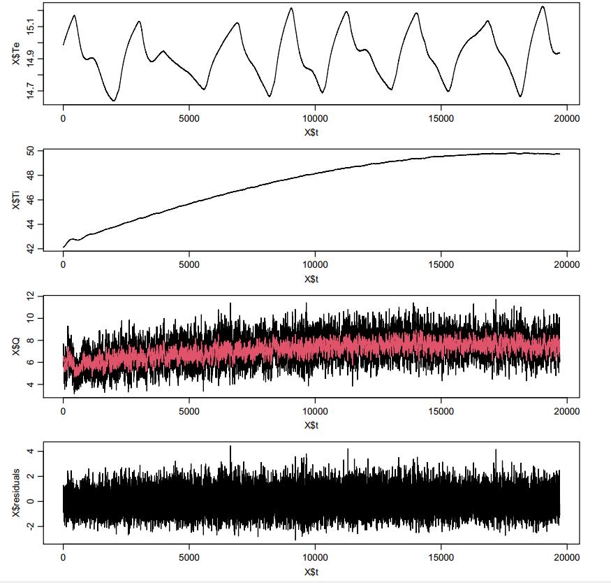
The number under the column estimate and Std.Error are the estimate value and the uncertainty of the parameter. Pr(>|t|) is the value The fraction of probability of the corresponding t distribution outside the limits set by the t value. Normally this value will smaller than 0.05, otherwise it means the model needs more inputs to estimate values. Next one value dF/dPar is also similar than Pr(>|t|), the value should be close to 0 or the result might not be the best solution, then some settings should be changed to repeat calculation. The last value shows the derivative of the penalty function with respect to the particular initial state or parameter. Then the estimate heat flux q will be used to compare with the real value to see if it is verified (the red line in the picture is the estimate value). The detail codes will be put in the Appendix D CTSM R code for dynamic tests. The dynamic test 2 simulation is showing in the figures below:
Figure 45 the simulation result for the assumed parameters
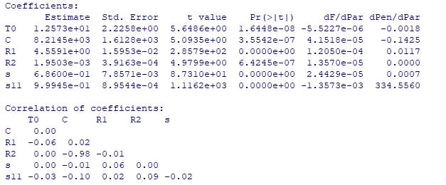
Figure 46 simulation conclusion images red line is the prediction heat flux R1 R2 C R (R1+R2) U Error
Test 1 4.41 0.76 17993 5.17 0.194 49% Test 2 4.56 1.95*10 3 8215 4.56 0.219 44% Test 3 4.53 2.52*10 3 6108 4.53 0.221 42% Theoretical value 2.5 0.13 12491 2.63 0.380
Table 13 test results summary of dynamic test 1 3 with theoretical value
Based on the result, although the U value for 3 tests are near the 0.2 the most of the previous tests, there are still some problems. The simulate thermal mass temperature in 3 tests are lower than the recorded temperature, the test 1 has lowest value, only 9.2℃ when the recorded temperature is 25.4℃. Dynamic test 1 simulation does not match the reference value and the heat flux simulation is complete different with the
measured value, the reason could be the long testing period includes the cooling phase, because there is no cooling system in the warm zone and this cause the temperature is dropping only rely on the heat loss through the sample wall; at same time, based on the result in the heat flux method test 10 11, the heat flux sensor can only sense very little voltage when all the heaters are shut down. The heat flux data is also an important value to confirm by the value of R1, and R1, R2 are basically calculated through the data of temperature difference between 2 sides. The simulate thermal mass temperature is also smaller than the measured temperature in all 3 tests, The dynamic tests 2 and 3 are a little better than test 1, the ratio between R1 and R2 is more matchable to the real result, although the R1 and R2 value is still not 100% correct. A manually calculation is also made rely on the recorded data, the R1 and R2 value is also mutual confirm the result. The thermal mass C in the test 1 has a very high reading, the value is over 18000 J/m2K and it is still has large dPEN/dPAR value means it can be higher, the test 2 and test 3’s result are smaller than 12491 J/m2K, but the reference value is also an approximately calculated based on the density and specific heat capacity of materials. The real thermal mass may need more accurate experiments to determine, for example the thermal mass flow meter. The detail data for 3 dynamic tests is in the Appendix G dynamic tests result
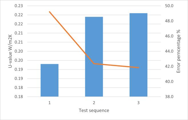 Figure 47 compare table dynamic tests
Figure 48 compare table dynamic tests with literature (literature 1 and 3 assumed the HFM value is the reference value)
4.5 Calibration of heat flux
In the case that almost all experimental results cannot be obtained close to the theoretical value, the heat flux sensor used in the test is suspected of being calibrated. The heat flux sensor calibration will be performed by the hot plate, an EPS board and the heat flux sensor.
In the hot plate, the heat flux sensor will be placed on the EPS board between the board and the hot side of hot plate. Data is transported through the USB cDAQ from the sensor to module, USB cDAQ and computer.
Figure 49 Settings for heat flux calibration
The test in the hot plate shows also wired reading from them the heat flux sensor. After turning on the hot plate, the heat flux sensor located on the EPS board facing the hot side should receive heat energy and generate the positive electricity signal, but according to the recorded data, the heat flux sensor always displays a pretty constant signal with 0.0005. The reason in this situation may because there is a connecting problem, since there is not enough time for further investigation, only further plan for calibration will be described.
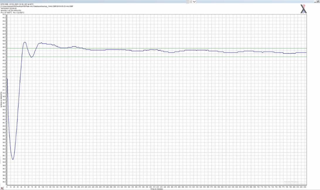
Figure 50 hot plate result picture during the heat flux calibration
Most of heat flux sensor calibration method are using the same laws of physics, the heat flux sensor will be placed on the heat conducting object, then the heat energy will go from the heater to the heat sink, the heating power used by heater will be recorded to divide the area of the heater can calculate the heat flux
ϕ= Pℎ���������� ��ℎ����������
Where:
Φ the heat flux W/m2
Pheater the power used for heater W
Aheater the heater surface area m2
The heat flux sensor sensitivity is the ration between the heat flux sensor output voltage and the applied heat flux Φ.
S= U������ ϕ
Where: S the heat flux sensor sensitivity μv
UHFM the output voltage of HFM μv/(W/m2)
Φ the applied heat flux W/m2
In (Huskseflux, 2018) it is mentioned the calibration settings based on (ASTM C113017, 2017) that the heat flux sensor (3) can be placed between a heater (2) and a solid material block (mass>1 kg) for calibration for example an aluminum block (5) An insulation layer (1) should be put on the heater to protect the heater and thermal energy. The heat flow (4) will be through the heat flux sensor from the heater to the metal block.
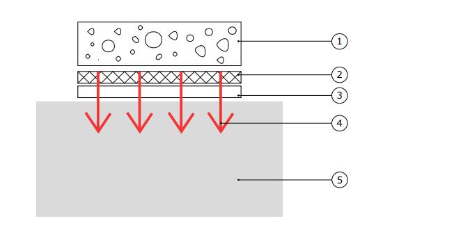
Figure 51 settings for simple heat flux calibration
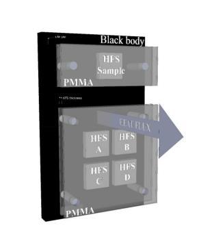
There are also other methods using different equipment, like (Tsai et al., 2004) states another method using the VTBB. The VTBB (variable-temperature blackbody) is using a thermally insulated graphite tube cavity heated by electricity. This method can heat tube very fast by using the large AC currents at low voltage. In (Jean, et al., 2014) described a method called MEC (Méthode Experimentale pour la Calibration” (in French)), this method will not directly place the sample heat flux on the black painted steel plate infrared bulb lamp but at 7cm for obtaining the more average flux. On another side of steel plate, there are 4 heat flux sensors fixed by the polymethyl
methacrylate and screws to also recorded the data and used for getting more accurate result Finally, the temperature sensors will be installed on both side of polymethyl methacrylate board and on the steel plate to measure the temperature during the test.
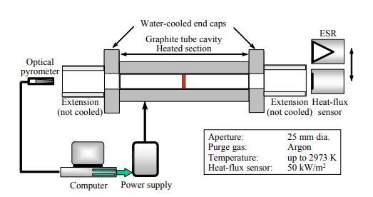
Figure 52 layout of VTBB
Figure 53 settings for MECr
5. Result and discussion
HFM method
Among all the HFM tests, the U value results with the smallest error are the HFM test 3 4, they have 0.23 W/m2K with 39.5% difference compare with the reference value
calculate based on hot plate data, this test also has the lowest heat flux standard deviation (42.3%,3σ) The worst (has biggest difference percentage) one test is HFM test 7, the heat flux standard deviation is also the biggest with 93% (3σ) in all the HFM test, these two tests also have the 2 smallest average heat flux value. In addition, it can be found in the data of HFM test 7 that when the cooling system was turned off, the heat flux reading was not only extremely unstable, but also oscillated around 0 within a period of time. This situation greatly interferes with the calculation of U value, making the final result seriously far away from the reference value.
Except the test 7 and test 8, most of HFM tests have a U value over 0.2 W/m2K. The HFM test 1 has only 0.18 W/m2K, compare with the similar condition test HFM test 2, according to the data that they have almost same average heat flux and standard deviation, the only one different parameter is the temperature difference between 2 sides (will call △T in the later parts) since the test 2 does not take the too high temperature reading in Zone 1, it makes the surface temperature in Zone 1 is smaller than the value in HFM test 1. Another one test has U value result smaller than 0.2 W/m2K is HFM test 6 SP 40. This test was done after dynamic test 1, the Zone 1 sensor 2 was placed into the EPS layer, and the other 2 PT100s were put closer to the middle area near the heat flux sensor. Compare the △T with test previous test, it can be found the △T is higher than the all the previous test when the set point is 40℃ in the warm side, this may be due to the fact that the remaining two thermometers are too close to the middle area and are directly heated by the heating device, which causes the high temperature reading. Too high temperature will also increase the temperature difference, so that the result of U value will also be smaller
In order to explore whether the higher temperature difference would affect the test results, the team conducted two sets of tests. They have all the same environmental factors except the set air temperature of the warm side, first one is 40 ℃ and the second one is 50 ℃ In the HFM test 4, 2 tests have a really close U value with 0.23 W/m2K, but the other parameters like the standard deviation of heat flux and temperature are smaller than the value under set point 40℃. In the HFM test 6, the U value is even better when the set point is 50℃ in Zone 1. In this set of comparative data, it can be observed that the heat flux and temperature standard deviation are almost same, the standard deviation of heat flux are 1.01 and 1.04, the temperature deviation are 0.19 and 0.14 In this case, according to the calculation equation of measured uncertainty, the one with the higher denominator (average value) will inevitably have a smaller percentage, resulting in more accurate data. These two sets of test data show that a higher temperature difference has a beneficial effect on the results, which can make the calculation results more accurate and have a smaller uncertainty value. However, whether it is possible to get closer to the reference value requires more experimental support.
IR test
Although IR test 1 does have the problem that the IR surface thermometer does not point to the target area, the error of the data is still unreasonable. The IR test 1 only has 0.126 W/m2K, the error of up to 25% from the reference value is mainly due to the high uncertainty of the heat flux. The other two experiments are relatively more reasonable and similar to most HFM test results. The two experiments are 0.21 W/m2K and 0.23 W/m2K. One of the more obvious problems in the three experiments is the surface temperature of the cold side. In IR test 1, the temperature of the cold side was always maintained at around 15.5℃ 16℃, while in IR tests 2 and 3, the temperature of the cold side was always maintained at 21.5 ℃ 22 ℃ Although the laser thermometer on the cold side of IR test 1 did not point to the area covered by the black electrical tape, according to subsequent tests, the temperature difference between the surface of the OSB board and the black electrical tape would not exceed 1 degree. Obviously, an experiment result was wrong when the temperature was 15 ℃ in 3 tests. In the dynamic test, the PT100 placed between the EPS board and the OSB board shows that the temperature is generally much higher than the cold side temperature. It can be inferred from dynamic temperature readings that the data of IR test 2 and 3 are more reasonable than IR test 1. Unfortunately, due to the shortage of manpower and time in experiment, further research and the influence of temperature difference on IR test cannot be carried out.
Dynamic test
The all 3 dynamic tests have the error percentage range from around 40% to 50%, dynamic test 3 has the lowest error 41.8% compare with reference value. The dynamic test 2 is a little bit higher than dynamic test 3, the U value is as same as dynamic test 1 value (0.22 W/m2K), the error is 42.4. The dynamic test 1 U value has the value almost half of the reference value. Different with test 1 has much bigger thermal mass value than the reference value, the test 2 and test 3 show 2 very small number, the test 2 thermal mass only has 8215 J/m2K and test 3 has the lowest 6108 J/m2K. The simulate thermal mass temperature area all bellowed the measured temperature, dynamic test 3 has the highest T0 temperature 19.7℃ but it is still smaller than the 27.3℃ based on the measured data. Dynamic test 1 simulated T0 is the smallest one which is 9.2 ℃, the one in the test is a little bit higher (12.6 ℃). Both have a too low simulate T0, even lower than the cold side air temperature, this will not happen which means the dynamic tests are failed.
The low T0 temperature and different cold side surface temperature between 2 IR tests also draw attention to the question: if the temperature readings are also affected by the cooling system. During the dynamic test, the measured thermal mass temperature is 10K higher than the cold side surface temperature, this caused a problem because there is only a layer of OSB board between the thermal mass temperature measured
PT100 and PT100s on cold side surface. According to the hot plate data, this thin layer cannot create so huge temperature difference with only 13mm thickness. This discovery led the team to suspect that the cold side surface PT100s was affected by the excessive cooling system. However, there is another explanation that the PT100 is not fixed between the two layers but stays in the EPS layers Unfortunately, since the limited manpower and time, this investigation could not be carried out.
Unstable heat flux readings inevitably make the calculation of U value more difficult and inaccurate. In addition, due to equipment limitations, the hot box cannot be closed properly, which is also suspected of causing negative effects.
If the three methods are compared based on the existing results, when the U value results calculated by the three methods are generally not much different (ignoring the failed tests like HFM test 7 and 8, IR test 1, dynamic test 1), U-value measurement by IR thermometer is the most suitable on site Useful. The IRT has the shortest testing time period by only 40 minutes. The single thermal mass method also shows a similar U value result, but it requires high level of theory understanding and numerical simulation ability, in addition, the dynamic test has longer test period than the IRT. The HFM has the longest test period and also the smallest error rate in 3 methods. HFM method can be used when the in situ U value measurement is the case where the goal is the closest to the real value, then the HFM should be used although it normally requires much more time to finish the test.
Compare with the literature, the tests made have much more error percentage than most of literature value, although some documents also show a high degree of error, most of the errors are less than the experimental value and are in the acceptable range.
Figure 54 compare table all tests with literatures
Paper name:
1. Comparative study of Hot Box Test Method using laboratory evaluation of thermal properties of a given building envelope system type
2. Energy performance of five different building envelope structures
3. A comparison of standardized calculation methods for in situ measurements of facades U value
4. In Situ Thermal Transmittance Measurements for investigating Differences between Wall Models and actual Building Performance
5. Validation of quantitative IR thermography for estimating the U value by a hot box apparatus
6. Find a modern and quick method to determine the U value and the thermal characteristics of a building envelope using an IR camera
7. Validation of quantitative IR thermography for estimating the U value by a hot box apparatus
8. Determining overall heat transfer coefficient (U Value) of wood framed wall assemblies in Canada using external infrared thermography
9. Application of infrared thermography for the determination of the overall heat transfer coefficient (U-Value) in building envelopes
10. Comparison of Infrared Thermography and Heat Flux Method for Dynamic Thermal transmittance Determination
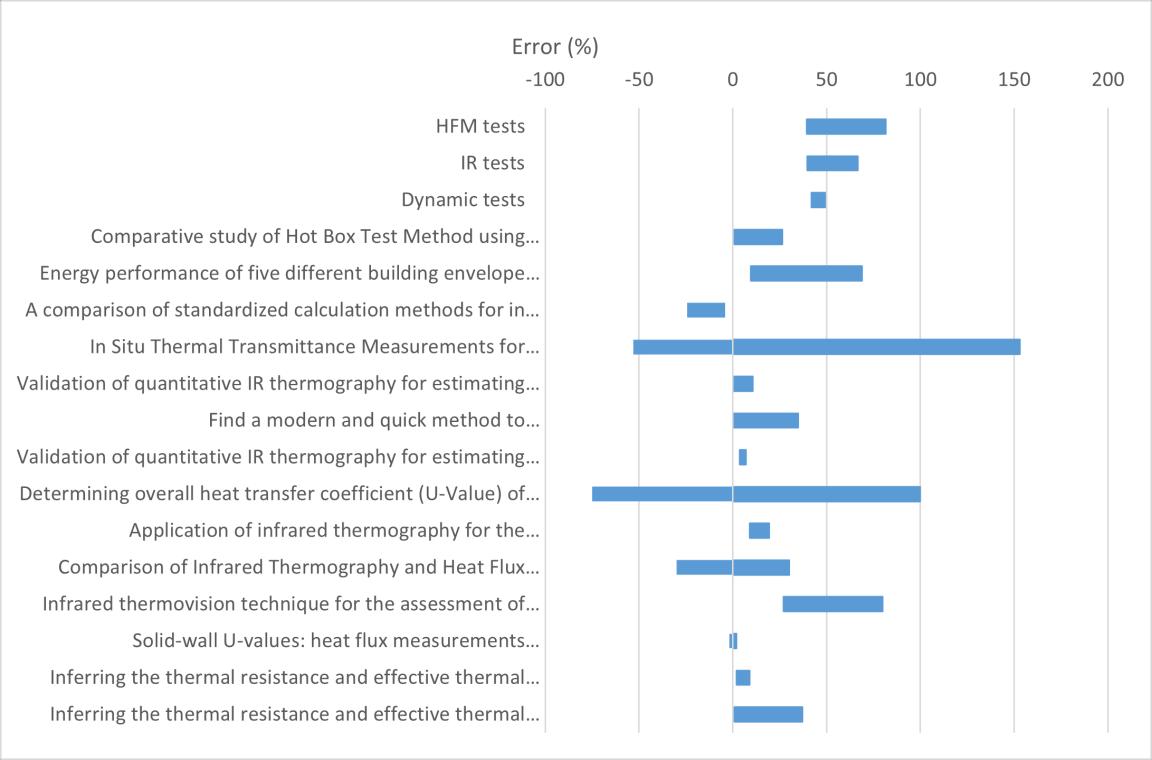
11. Infrared thermo vision technique for the assessment of thermal transmittance value of opaque building elements on site
12. Solid wall U values: heat flux measurements compared with standard assumptions
13. Inferring the thermal resistance and effective thermal mass distribution of a wall
from in situ measurements to characterise heat transfer at both the interior and exterior surfaces
14. Inferring the thermal resistance and effective thermal mass of a wall using frequent temperature and heat flux measurements
6.Conclusion
In the case of using hot plate data and ISO standard calculation results as true reference values, after using different methods to perform U value measurements on the same sample wall to obtain a certain amount of data and refer to other research materials, according to the results, it can be concluded that when the in situ measurement is aimed at fast and efficient, IRT is the most suitable Methods. IRT does not need to install many instruments, and the experiment time is the shortest. When the goal is to get the closest true reference value (calculate according to ISO standard), HFM can have smaller errors than IRT, although HFM is the longest time consuming method. The dynamic method has the advantages of both short time and high enough accuracy. When the n situ measurement has high level personnel with enough ability to finish more complex calculations, the dynamic method can complete the experiment within a few hours and obtain a sufficiently accurate value. It can be observed in multiple tests that the heat flux can have a very large impact on the U value calculation results, especially in the HFM test, when the temperature difference between the two sides of the hot box stabilizes, the uncertainty of U value is mainly caused by unstable heat flux readings. In IRT testing and dynamic methods, temperature also affects the experimental results. In dynamic testing, some suspected wrong temperature data will cause the simulation results to be very different from the actual measured values. In addition, some experimental equipment problems should not be ignored, such as the poor performance and optional functions of the IR thermometer 2. Mistakes in some experiments also have an impact on the experiment, causing the experiment to fail or increase the error. Two HFM control experiments proved that a higher temperature difference can effectively reduce the uncertainty of the experimental results. It is not yet confirmed whether it will also affect U value and other methods.
Due to the shortage of manpower and time, some tests cannot be further explored, such as IR test and dynamic test with higher temperature difference. The thermal mass required in the dynamic experiment should be measured with a special instrument. If the estimated thermal mass is correct, it should be checked whether the formula used in the simulation software is correct and the PT100 can correctly measure the surface temperature of the sample wall. The heat flux sensor needs also further calibration to ensure the data from it is correct and accurate. If the temperature and heat flux are corrected, then the hot box should be checked to exclude any influence from gaps or
holes that may exist. In the IR tests, the IR thermometers can be switched to another side to verify the pervious data is correct, especially for the cold side sample wall surface temperature. If possible, the IR thermometer should use the power cord as the energy supply method instead of the battery. It is not possible to use the battery IR thermometer for a long time at high temperatures.
List of reference
Harvard University, 2007. A Summary of Error Propagation. Available at: http://ipl.physics.harvard.edu/wp uploads/2013/03/PS3_Error_Propagation_sp13.pdf
A Francois et al, 2019. Building thermal bridge heat losses quantification by infrared thermography. Steady state evaluation and uncertainty calculation.
Andrew Stone et al., 2014. Key factors determining the energy rating of existing English houses. 2 5.
Arash, R., 2020. In Situ Determination of Buildings’ Thermo Physical Characteristics, s.l.: s.n.
ASTM C1130 17, 2017. ASTM C1130 17.
Australian Urethane & Styrene, n.d. Expanded Polystyrene. Available at: https://www.thermalps.com.au/imagesDB/wysiwyg/TDS_Expanded_Polystyrene.pdf
B. e. a., 2014. Inferring the thermal resistance and effective thermal mass of a wall using frequent temperature and heat flux measurements]. 8.
Czajkowski, Ł., Olek, W., Weres, J. & Guzenda , R., 2016. Thermal properties of wood based panels: specific heat determination.
Danielski, I. & Fröling, M., 2015. Diagnosis of Buildings’ Thermal Performance A Quantitative Method Using Thermography Under Non steady State Heat Flow. 12. Desogus, G., Mura, S. & Ricciu, R., 2010. Comparing different approaches to in situ measurement of building components.
Engineering ToolBox, 2003. Specific Heat of common Substances. Available at: https://www.engineeringtoolbox.com/specific heat capacity d_391.html European Commission , 2020. European Commission. Available at: https://ec.europa.eu/info/energy climate change environment_en Fokaides, P. A. & Kalogirou, S. A., 2011. Application of infrared thermography for the determination of the overall heat.
Fokaides, P. A. & Kalogirou, S. A., 2011. Application of infrared thermography for the determination of the overall heat.
Gaspar, K., Casals, M. & Gangolells, M., 2016. A comparison of standardized calculation methods for in situmeasurements of fac ades U value.
Gori, V., Biddulph, P., Elwell, C. A. & Marincioni, V., 2016. Inferring the thermal resistance and effective thermal mass distribution of a wall from in situ measurements to characterise heat transfer at both the interior and exterior surfaces.
Green teg, 2018. Instruction Manual for gSKIN® Heat Flux Sensors. Available at: https://greenteg.com/template/userfiles/files/gSKIN_Heat%20Flux%20Sensors%20R %26D_Instructions_v3.pdf
Huskseflux, 2018. USER MANUAL FHF02SC.
Available at: https://www.hukseflux.com/uploads/product documents/FHF02SC_manual_v1803.pdf
ISO 6946, 2017. ISO 6946.
Available at: https://www.iso.org/standard/65708.html
ISO 7345, 2018. https://www.iso.org/standard/65000.html. [联机].
ISO 8990, 1994. ISO 8990:1994
ISO 9869, 2014. ISO 9869.
Jean, A., Craig, A., Miranville, F. & Medina, M., 2014. Experimental Method Calibration (MECr): A new relative method for heat flux sensor calibration. 7 12. Johra, H., 2019. Description of the Guarded Hot Plate Method for Thermal Conductivity Measurement with the EP500
Li et al, 2014. Solid wall U values: heat flux measurements. 16 10. Material Properties, 2021. Polystyrene Density Strength Melting Point Thermal Conductivity.
Available at: https://material properties.org/polystyrene density strength melting point thermal conductivity/ Mergim Gaši, B. M. S. G., 2019. Comparison of Infrared Thermography and Heat Flux Method for Dynamic Thermal Transmittance Determination
Rasooli, A. & Itard, . L. C. M., 2016. Introduction to an In situ Method for Rapid Measurement of the Walls’ Thermal Resistance in Existing Buildings, s.l.: s.n. T. e. a., 2004. NIST MEASUREMENT SERVICES:Heat Flux Sensor Calibration, s.l.: s.n. TRADA, 2014. Panel Guide.
Available at: https://wpif.org.uk/uploads/PanelGuide/PanelGuide_2014_Annex2B.pdf
University of Iowa, 2017. Imaging the Universe.
Available at: http://astro.physics.uiowa.edu/ITU/courses/general-astronomy/erroranalysis/formulae for statistics and.html
List of figures
Figure 1 sketch of the sample wall ..................................................................... 7
Figure 2 cooling pipes for the hot box 8
Figure 3 the control cabinet of hot box .............................................................. 9
Figure 4 interface of the VI 10
Figure 5 a loop in the back page....................................................................... 10
Figure 6 the hot plate used in the experiment ................................................. 14
Figure 7 Location of the field of measurement, soft insulating materials (left), hard non insulating materials + guarding insulation frame (Johra, 2019).......... 16
Figure 8 cross section of hot box in the test ..................................................... 19
Figure 9 PT100 calibration example 20
Figure 10 the chosen data area........................................................................ 21
Figure 11 the U value data test 1 ..................................................................... 22
Figure 12 the heat flux data HFM test 1 22
Figure 13 the surface temperature data HFM test 1........................................ 22
Figure 14 the U value data HFM test 2(after) 23
Figure 15 the heat flux data HFM test 2(after) ................................................ 24
Figure 16 the surface temperature data HFM test 2(after).............................. 24
Figure 17 the U value data HFM test 3.1 25
Figure 18 the heat flux data HFM test 3.1....................................................... 25
Figure 19 the surface temperature data HFM test 3.1 .................................... 26
Figure 20 the U value data HFM test 3.2 26
Figure 21 the heat flux data HFM test 3.2....................................................... 27
Figure 22 the surface temperature data HFM test 3.2 .................................... 27
Figure 23 the U value data HFM test 4.40 28
Figure 24 the heat flux data HFM test 4.40 ..................................................... 29
Figure 25 the surface temperature data HFM test 4.40 29
Figure 26 the U value data HFM test 4.50....................................................... 29
Figure 27 the heat flux data HFM test 4.50 ..................................................... 30
Figure 28 the surface temperature data HFM test 4.50 30
Figure 29 cover on the heat flux sensor ........................................................... 31
Figure 30 paper fabric cover in the hot box...................................................... 32
Figure 31 heat flux oscillation after turn off the heating system 34
Figure 32 compare table HFM tests ................................................................ 35
Figure 33 Error rate HFM tests compare with literature 35
Figure 34 picture during IR test 2 37
Figure 35 Laser thermometer 1 calibration ...................................................... 38
Figure 36 IR test 2 cold zone surface temperature 40
Figure 37 the heat flux data IR test 2 .............................................................. 40
Figure 38 the heat flux data IR test 3.............................................................. 40
Figure 39 thermal Imaging of sample wall right after a test.............................. 41
Figure 40 compare table laser thermometer tests 41
Figure 41 compare table- laser tests with literature ......................................... 42
Figure 42 the surface temperature during the dynamic test 1 .......................... 45
Figure 43 surface temperature data for analyzing dynamic test 1 45
Figure 44 surface temperature data for analyzing dynamic test 2................... 46
Figure 45 the simulation result for the assumed parameters............................ 47
Figure 46 simulation conclusion images red line is the prediction heat flux 47
Figure 47 compare table dynamic tests........................................................... 48
Figure 48 compare table dynamic tests with literature (literature 1 and 3 assumed the HFM value is the reference value) 49
Figure 49 Settings for heat flux calibration ....................................................... 50
Figure 50 hot plate result picture during the heat flux calibration 50
Figure 51 settings for simple heat flux calibration ............................................ 51
Figure 52 layout of VTBB.................................................................................. 52
Figure 53 settings for MECr 52
Figure 54 compare table all tests with literatures............................................ 56
Figure A 1 settings in EP500 67
Figure A 2 EPS board result in EP500................................................................ 68
Figure A 3 OSB board result in EP500............................................................... 69
Figure A 4 EP500 result for 2 layers 70
Figure B 1 precision thermometer F200 71
Figure B 2 Isocal-6............................................................................................ 71
Figure B 3 calibration formula OPZ1S1 ............................................................. 72
Figure B 4 calibration formula OPZ1S2 72
Figure B 5 calibration formula OPZ3S1 ............................................................. 73
Figure B 6 calibration formula OPZ3S2 73
Figure B 7 calibration formula SZ1S1................................................................ 73
Figure B 8 calibration formula SZ1S2................................................................ 74
Figure B 9 calibration formula SZ1S3................................................................ 74
Figure B 10 calibration formula SZ3S1 74
Figure B 11 calibration formula SZ3S2.............................................................. 75
Figure B 12 calibration formula SZ3S3 75
Figure C 1 calibration formula IR thermometer 1 ............................................. 76
Figure C 2 calibration formula IR thermometer 1 77
Figure E 1 U value data 1 83
Figure E 2 heat flux data 1 .............................................................................. 83
Figure E 3 surface temperature data 1 ............................................................ 84
Figure E 4 U value data 2.1............................................................................. 84
Figure E 5 heat flux data 2.1 85
Figure E 6 surface temperature data 2.1 ........................................................ 85
Figure E 7 U value data– 2.2............................................................................. 86
Figure E 8 heat flux data 2.2 86
Figure E 9 surface temperature data 2.2 ........................................................ 87
Figure E 10 U value data 3.1.......................................................................... 88
Figure E 11 heat flux data 3.1 88
Figure E 12 surface temperature data 3.1...................................................... 89
Figure E 13 U value data 3.2.......................................................................... 89
Figure E 14 heat flux data 3.2 90
Figure E 15 surface temperature data 3.2...................................................... 90
Figure E 16 U value data 4.40 91
Figure E 17 heat flux data 4.40....................................................................... 91
Figure E 18 surface temperature data– 4.40..................................................... 91
Figure E 19 U value data 4.50 92
Figure E 20 surface temperature data 4.50..................................................... 92
Figure E 21 heat flux data 4.50 93
Figure E 22 U value data 5 93
Figure E 23 heat flux data 5............................................................................ 94
Figure E 24 surface temperature data 5 ......................................................... 94
Figure E 25 U value data 6.40 95
Figure E 26 heat flux data 6.40....................................................................... 95
Figure E 27 surface temperature data 6.40 96
Figure E 28 U-value data 6.50......................................................................... 96
Figure E 29 heat flux data– 6.50....................................................................... 97
Figure E 30 surface temperature data 6.50 97
Figure E 31 U value data 7 ............................................................................. 98
Figure E 32 heat flux data 7 98
Figure E 33 surface temperature data 7 ......................................................... 99
Figure E 34 overall heat flux condition after turned off the cooler in 1h 7 ...... 99
Figure E 35 U value data HFM 8................................................................... 100
Figure E 36 heat flux data 8 100
Figure E 37 surface temperature data 8 ....................................................... 101
Figure E 38 The overall situation when turn off the heater 8 101
Figure E 39 heat flux data OT1..................................................................... 102
Figure E 40 U value data – OT1 ...................................................................... 102
Figure E 41 surface temperature data OT1 102
Figure E 42 U value data OT2........................................................................ 103
Figure E 43 heat flux data OT2 103
Figure E 44 surface temperature data OT2.................................................... 104
Figure E 45 overall heat flux data OT2........................................................... 104
Figure F 1 IR test 1 surface temperature data 105
Figure F 2 IR test 1 compare data heat flux and U-value................................. 106
Figure F 3 IR test 2 compare data heat flux and U value................................. 107
Figure F 4 IR test 2 surface temperature data 107
Figure F 5 IR test 3 compare data heat flux and U value................................. 108
Figure F 6 IR test 3 surface temperature data................................................. 108
Figure G 1 input data dynamic 1 .................................................................... 109
Figure G 2 simulate parameter value dynamic 1 ............................................ 110
Figure G 3 simulate value compare with real value dynamic 1 110
Figure G 4 ACF residuals dynamic 1 ............................................................... 111
Figure G 5 final result with estimate heat flux dynamic 1 112
Figure G 6 input data-dynamic 2 .................................................................... 113
Figure G 7 simulate parameter value dynamic 2 ............................................ 113
Figure G 8 simulate value compare with real value dynamic 2 114
Figure G 9 ACF residuals dynamic 2 ............................................................... 114
Figure G 10 final result with estimate heat flux dynamic 2 115
Figure G 11 input data dynamic 3 116
Figure G 12 simulate parameter value dynamic 3 .......................................... 116
Figure G 13 simulate value compare with real value dynamic 3 ..................... 117
Figure G 14 ACF residuals dynamic 3 117
Figure G 15 final result with estimate heat flux dynamic 3 ............................. 118
Figure H 1 IR camera photo 1: HFM................................................................ 119
Figure H 2 IR camera photo 1: reference photo.............................................. 119
Figure H 3 IR camera photo 2: corner 120
Figure H 4 IR camera photo 2: reference photo.............................................. 120
Figure H 5 IR camera photo 3: fixture 121
Figure H 6 IR camera photo 3: reference photo.............................................. 121
Figure H 7 IR camera photo 4:fixture and heat flux sensor ............................. 122
Figure H 8 IR camera photo 4: reference photo.............................................. 122
Figure H 9 IR camera photo 5: right side corner and fixture 123
Figure H 10 IR camera photo 5: reference photo............................................ 123
List of tables
Table 1 devices table........................................................................................ 19
Table 2 test results summary of HFM test 1 21
Table 3 test results summary of HFM test 2 ..................................................... 23
Table 4 test results summary of HFM test 3 28
Table 5 test results summary of HFM test 4 ..................................................... 30
Table 6 test results summary of HFM test 5 6 .................................................. 32
Table 7 heat flux placement in Zone 3 33
Table 8 test results summary of HFM test 7 8 .................................................. 34
Table 9 IR test devices table ............................................................................. 37
Table 10 different type of light 38
Table 11 test results summary of IR test 1 3..................................................... 39
Table 12 dynamic test settings and sketch........................................................ 44
Table 13 test results summary of dynamic test 1 3 with theoretical value 47
Table E 1 HFM test result 1 83
Table E 2 HFM test result 2.1......................................................................... 84
Table E 3 HFM test result 2.2......................................................................... 85
Table E 4 HFM test result 3.1 87
Table E 5 HFM test result 3.2......................................................................... 89
Table E 6 HFM test result 4.40....................................................................... 91
Table E 7 HFM test result 4.50 92
Table E 8 HFM test result 5 ............................................................................ 93
Table E 9 HFM test result 6.40....................................................................... 95
Table E 10 HFM test result 6.50 96
Table E 11 HFM test result 7........................................................................... 97
Table E 12 HFM test result 8 99
Table E 13 HFM test result OT1 ................................................................... 101
Table E 14 HFM test result OT1 ................................................................... 103
Table F 1 detail IR test 1 data ......................................................................... 105
Table F 2 IR test 1result.................................................................................. 105
Table F 3 detail IR test 2 data 106
Table F 4 IR test 2 result ................................................................................. 106
Table F 5 detail IR test 3 data 107
Table F 6 IR test 3 result 108
Enclosures
Appendix A- hot plate measurement
Hot plate test 1
Equipment and setup
• Guarded hot plate
• wooden plate 15 cm x 15 cm, 1.2 cm thick
• EPS board 50 cm x 50 cm, 10 cm thick
Settings for the test: 0.3 % and 600 min time 15 K temp. difference between the plates
Figure A 1 settings in EP500
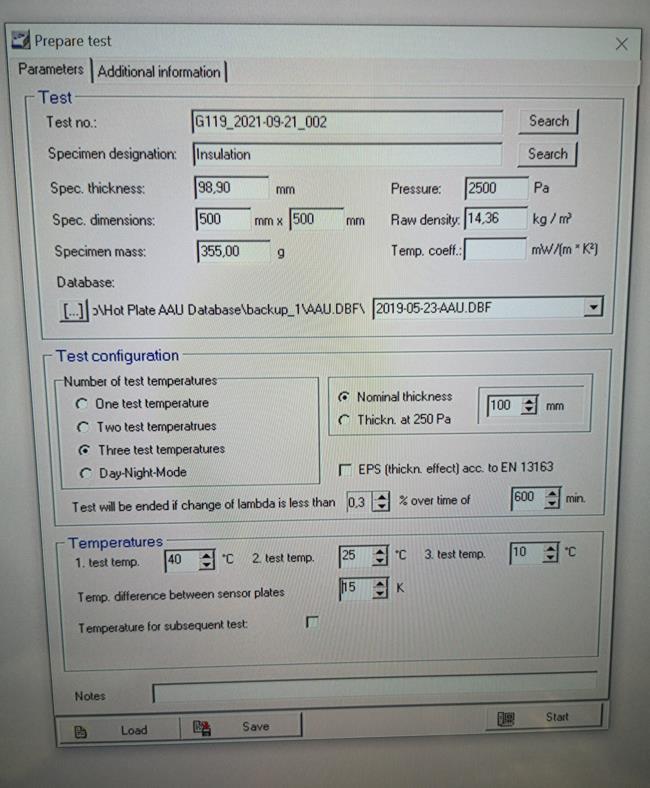
The 2 different materials were tested separately, first one is EPS board.
Results for the EPS:
Figure A 2 EPS board result in EP500 lambda value:
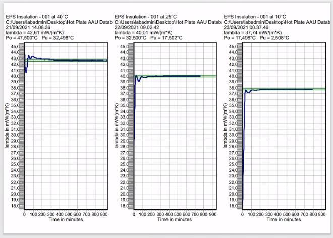
• at 40 °C: λ = 42.61 mW/m*K;
• at 25 °C: λ = 40.01 mW/m*K;
• at 10 °C: λ = 37.74 mW/m*K.
aver.: 40.12 mW/m*K = 0.04 W/m*K
Results for OSB board:
Figure A 3 OSB board result in EP500
lambda value:
• at 40 °C: λ = 92.27 mW/m*K;
• at 25 °C: λ = 87.85 mW/m*K;
• at 10 °C: λ = 85 mW/m*K.
aver.: 88.37 mW/m*K = 0.088 W/m*K
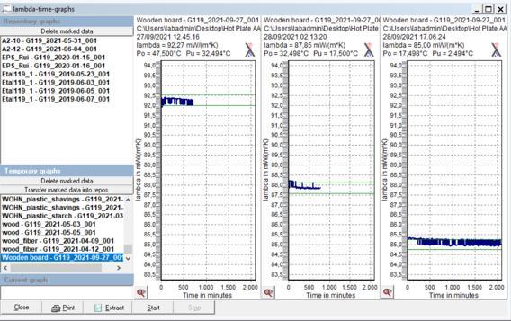
The total R value for both layer equal to: 0.1/0.04+0.012/0.088=2.63 W/m*K
The U value for both layer equal to: 1/2.63=0.38 W/m2*K
Figure A 4 EP500 result for 2 layers
The average R value for 2 layers is (2.53+2.69+2.85)/3=2.69 W/m*K U=1/R=0.37 W/m2*K
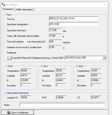
Hot
test 2
plate
Appendix B- PT100s calibration
Calibration of the Pt100s
In order to get precise readings during measurements, the instruments should be calibrated. This chapter presents the calibration of Pt100s used in the hot box measurements.
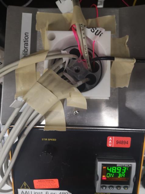
Equipment and setup
• Pt100s temperature probes (10 pieces)
• precision thermometer F200
• multifunction temperature calibration system Isocal 6
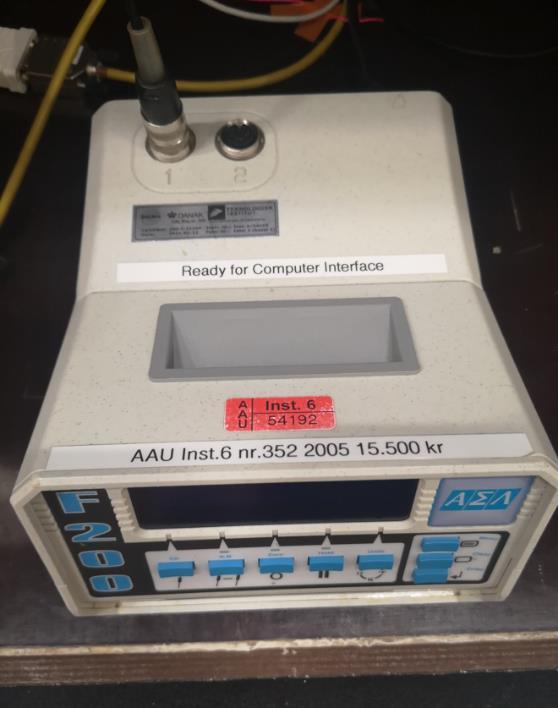
• paper and tape for insulation
• Computer with LabVIEW
Figure B 2 Isocal 6
Figure B 1 precision thermometer F200
Set up for the calibration: Pt100s in the Isocal 6 chamber and the F200 to the right
Measurements
First the Pt100s were put in the chamber of Isocal 6, secured with tape, and covered
with some paper for insulation from the outside temperature. Then Isocal 6 was used to generate temperature which was then measured with the precise thermometer resulting in getting the real reference temperature. Four temperature points were set: 10 °C, 25 °C, 45 °C, 60 °C. For each point the procedure was the same: once the temperature stabilized in the Isocal 6, the value on F200 and on each Pt100 was read and both values were plotted in the graph. After repeating the measurement for all 4 temperature points calibration curves were created, as seen in figures below. The graphs show also a calibration equation for each Pt100.
Mod1 Chan 3: Op temp zone 1 sensor 1
y = 0.9887x + 0.1327 10 15 20 25 30 35 40 45 50 55 60 65 10.00 15.00 20.00 25.00 30.00 35.00 40.00 45.00 50.00 55.00 60.00 65.00
reference temp. [C] measured temp. [C]
Figure B 3 calibration formula OPZ1S1
Mod1 Chan 4: Op temp zone 1 sensor 2
y = 0.9944x + 0.1877 10 15 20 25 30 35 40 45 50 55 60 65 10.00 15.00 20.00 25.00 30.00 35.00 40.00 45.00 50.00 55.00 60.00 65.00
reference temp. [C] measured temp. [C]
Figure B 4 calibration formula OPZ1S2
Mod1 Chan 5: Op temp zone 3 sensor 1
y = 1.0047x 0.3148 10 15 20 25 30 35 40 45 50 55 60 65 10.00 15.00 20.00 25.00 30.00 35.00 40.00 45.00 50.00 55.00 60.00 65.00
reference temp. [C] measured temp. [C]
Figure B 5 calibration formula OPZ3S1
Mod1 Chan 6: Op temp zone 3 sensor 2
y = 1.0164x 0.5701 10 15 20 25 30 35 40 45 50 55 60 65 10.00 15.00 20.00 25.00 30.00 35.00 40.00 45.00 50.00 55.00 60.00 65.00
reference temp. [C] measured temp. [C]
Figure B 6 calibration formula OPZ3S2
Mod4 Chan 3: Surf temp test sample zone 1 sensor 1
y = 1.0388x 0.9618 10 15 20 25 30 35 40 45 50 55 60 65 10.00 15.00 20.00 25.00 30.00 35.00 40.00 45.00 50.00 55.00 60.00 65.00
reference temp. [C] measured temp. [C]
Figure B 7 calibration formula SZ1S1
Mod4 Chan 4: Surf temp test sample zone 1 sensor 2
y = 1.0273x 0.7009 10 15 20 25 30 35 40 45 50 55 60 65 10.00 15.00 20.00 25.00 30.00 35.00 40.00 45.00 50.00 55.00 60.00 65.00
reference temp. [C] measured temp. [C]
Figure B 8 calibration formula SZ1S2
Mod4 Chan 5: Surf temp test sample zone 1 sensor 3
y = 1.0289x 0.7193 10 15 20 25 30 35 40 45 50 55 60 65 10.00 15.00 20.00 25.00 30.00 35.00 40.00 45.00 50.00 55.00 60.00 65.00
reference temp. [C] measured temp. [C]
Figure B 9 calibration formula SZ1S3
Mod4 Chan 6: Surf temp test sample zone 3 sensor 1
y = 1.0173x 0.3591 10 15 20 25 30 35 40 45 50 55 60 65 10.00 15.00 20.00 25.00 30.00 35.00 40.00 45.00 50.00 55.00 60.00 65.00
reference temp. [C] measured temp. [C]
Figure B 10 calibration formula SZ3S1
Mod4 Chan 7: Surf temp test sample zone 3 sensor 2
y = 1.0192x 0.4214 10 15 20 25 30 35 40 45 50 55 60 65
reference temp. [C] measured temp. [C]
10.00 15.00 20.00 25.00 30.00 35.00 40.00 45.00 50.00 55.00 60.00 65.00
Figure B 11 calibration formula SZ3S2
Mod4 Chan 8: Surf temp test sample zone 3 sensor 3
y = 1.0309x 0.5584 10 15 20 25 30 35 40 45 50 55 60 65 10.00 15.00 20.00 25.00 30.00 35.00 40.00 45.00 50.00 55.00 60.00 65.00
reference temp. [C] measured temp. [C]
Figure B 12 calibration formula SZ3S3
Results
Calibration can be done either before the measurements, or after as long as the calibration equation is used to calculate the real temperature. In the case of this project the precision thermometer was not available for some time and therefore it was decided to do the measurements in the hot box first and to perform the calibration afterwards, once F200 is available. The obtained calibration equations were applied later to calculations to get the real temperature readings of the Pt100s. It can be seen that the Pt100s are precise since the equations are not much different than ax + b.
Appendix C- IR thermometer calibration
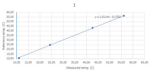
Calibration of the infrared thermometers
In order to get precise readings during measurements, the instruments should be calibrated. This chapter presents the calibration of the two no contact thermometers used in the hot box measurements.
Equipment and setup
• 2 infrared thermometers: AMIR 7811 and Thermo Control I, Infrarot
• precision thermometer F200
• multifunction temperature calibration system Isocal 6
• paper and tape for insulation
• Computer with LabVIEW
Measurements
First the temperature probe from F200 was placed in the chamber of Isocal 6 and covered with some paper for insulation from the outside temperature. Then Isocal 6 was used to generate temperature which was then measured with the precise thermometer for getting the real reference temperature. The plan was for four temperature points: 10 °C, 25 °C, 45 °C, 60 °C. For each point the procedure was the same: once the temperature stabilized in the Isocal 6, the value on F200 and on each infrared thermometer was read and the values were plotted in the graph. Figure C 1 calibration formula IR thermometer 1
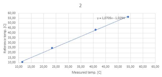 Figure C 2 calibration formula IR thermometer 1
Appendix D- CTSM-R code for dynamic tests
The code for dynamic test 1 is listing below:
## Set the working directory setwd(".")
## Use the ctsmr package library(ctsmr) library(readxl)
## Initialize the model model < ctsm$new()
## Specify the system equations model$addSystem(dT ~ ( 1/(C*R1) * (Ti T) + 1/(C*R2) * (Te T) ) * dt + s11* dw)
## The inputs model$addInput("Te","Ti")
## The observation equation model$addObs( Q ~ 1/R1*(Ti T)) model$setVariance(Q ~ s)
model$setParameter( T0 = c(init=20.2 ,lb=8 ,ub=40 )) model$setParameter( C = c(init=10000 ,lb=8000 ,ub=18000) ) model$setParameter( R1 = c(init=2 ,lb=0 ,ub=5 ) ) model$setParameter( R2 = c(init=2 ,lb=0 ,ub=5 ) ) model$setParameter( s11 = c(init=0.01 ,lb=0 ,ub=1 ) ) model$setParameter( s = c(init=0.01 ,lb=0 ,ub=1 ) )
X < read_excel(file.choose(), sheet = "Sheet1", skip = 0) X < subset (X , select = c("t","Ti","Te","T","Q")) print(X)
par(mfrow=c(3,1),mar=c(3,3.5,1,1),mgp=c(2,0.7,0)) # Setup plot plot(X$t,X$Te,type="l") plot(X$t,X$Ti,type="l") plot(X$t,X$Q,type="l") fit < model$estimate(X)
## Print the parameters estimates and the Correlation Matrix of the estimates summary(fit,extended=TRUE)
## The parameter estimates in a data.frame Prm < data.frame(xm=fit$xm) row.names(Prm) < names(fit$xm)
## The true parameter values Prm$xmtrue < c(20.2,12491,2.6,0.006,0.01,0)
## Approximately lower 95% confidence bound Prm$lower < (fit$xm 3*fit$sd)
## Approximately upper 95% confidence bound Prm$upper < (fit$xm + 3*fit$sd)
## Print it all ##round(Prm,digits=2) format(Prm,digits=4)
## Calculate the one step ahead predictions tmp < predict(fit, newdata=X)
## Calculate the residuals and put them with the data in a data.frame X X$QHat <- tmp$output$pred$Q
X$residuals < X$Q X$QHat
## Auto correlation function and cumulated periodogram par(mfrow=c(1,2))
#Setup plot acf(X$residuals) cpgram(X$residuals)
## Plot of inputs, output, one step ahead predicted output, and residuals par(mfrow=c(4,1),mar=c(3,3.5,1,1),mgp=c(2,0.7,0)) # Setup plot plot(X$t,X$Te,type="l") plot(X$t,X$Ti,type="l") plot(X$t,X$Q,type="l") lines(X$t,X$QHat,col=2) plot(X$t,X$residuals,type="l")
The code for dynamic test 2 is listing below:
## Set the working directory setwd(".")
## Use the ctsmr package library(ctsmr) library(readxl)
## Initialize the model model < ctsm$new()
## Specify the system equations model$addSystem(dT ~ ( 1/(C*R1) * (Ti T) + 1/(C*R2) * (Te T) ) * dt + s11* dw)
## The inputs model$addInput("Te","Ti")
## The observation equation model$addObs( Q ~ 1/R1*(Ti T)) model$setVariance(Q ~ s)
model$setParameter( T0 = c(init=27 ,lb=10 ,ub=35 )) model$setParameter( C = c(init=10000 ,lb=8000 ,ub=15000) ) model$setParameter( R1 = c(init=2 ,lb=0 ,ub=5 ) ) model$setParameter( R2 = c(init=2 ,lb=0 ,ub=5 ) ) model$setParameter( s11 = c(init=0.01 ,lb=0 ,ub=1 ) ) model$setParameter( s = c(init=0.01 ,lb=0 ,ub=1 ) )
X < read_excel(file.choose(), sheet = "Sheet1", skip = 0)
X < subset (X , select = c("t","Ti","Te","T","Q")) print(X)
par(mfrow=c(3,1),mar=c(3,3.5,1,1),mgp=c(2,0.7,0)) # Setup plot plot(X$t,X$Te,type="l") plot(X$t,X$Ti,type="l") plot(X$t,X$Q,type="l") fit < model$estimate(X)
## Print the parameters estimates and the Correlation Matrix of the estimates summary(fit,extended=TRUE)
## The parameter estimates in a data.frame Prm < data.frame(xm=fit$xm)
row.names(Prm) < names(fit$xm)
## The true parameter values Prm$xmtrue < c(27.4,12491,2.6,0.01,0.01,0)
## Approximately lower 99% confidence bound Prm$lower < (fit$xm 3*fit$sd)
## Approximately upper 99% confidence bound Prm$upper < (fit$xm + 3*fit$sd)
## Print it all ##round(Prm,digits=2) format(Prm,digits=6)
## Calculate the one step ahead predictions tmp < predict(fit, newdata=X)
## Calculate the residuals and put them with the data in a data.frame x X$QHat < tmp$output$pred$Q X$residuals < X$Q X$QHat
## Auto correlation function and cumulated periodogram par(mfrow=c(1,2))
#Setup plot acf(X$residuals) cpgram(X$residuals)
## Plot of inputs, output, one step ahead predicted output, and residuals par(mfrow=c(4,1),mar=c(3,3.5,1,1),mgp=c(2,0.7,0)) # Setup plot plot(X$t,X$Te,type="l") plot(X$t,X$Ti,type="l") plot(X$t,X$Q,type="l") lines(X$t,X$QHat,col=2) plot(X$t,X$residuals,type="l")
Test 3:
# Set the working directory setwd(".")
## Use the ctsmr package library(ctsmr) library(readxl)
## Initialize the model model < ctsm$new()
## Specify the system equations model$addSystem(dT ~ ( 1/(C*R1) * (Ti T) + 1/(C*R2) * (Te T) ) * dt + s11* dw)
## The inputs model$addInput("Te","Ti")
## The observation equation model$addObs( Q ~ 1/R1*(Ti T)) model$setVariance(Q ~ s)
model$setParameter( T0 = c(init=27.2 ,lb=10 ,ub=40 )) model$setParameter( C = c(init=10000 ,lb=6000 ,ub=20000) )
model$setParameter( R1 = c(init=2 ,lb=0 ,ub=6 ) ) model$setParameter( R2 = c(init=0.1 ,lb=0 ,ub=5 ) ) model$setParameter( s11 = c(init=0.01 ,lb=0 ,ub=1 ) ) model$setParameter( s = c(init=0.01 ,lb=0 ,ub=1 ) )
X < read_excel(file.choose(), sheet = "Sheet1", skip = 0)
X < subset (X , select = c("t","Ti","Te","T","Q")) print(X)
par(mfrow=c(3,1),mar=c(3,3.5,1,1),mgp=c(2,0.7,0)) # Setup plot
plot(X$t,X$Te,type="l") plot(X$t,X$Ti,type="l") plot(X$t,X$Q,type="l") fit < model$estimate(X)
## Print the parameters estimates and the Correlation Matrix of the estimates summary(fit,extended=TRUE)
## The parameter estimates in a data.frame Prm < data.frame(xm=fit$xm) row.names(Prm) < names(fit$xm)
## The true parameter values Prm$xmtrue < c(27.4,12491,2.6,0.006,0.01,0)
## Approximately lower 95% confidence bound Prm$lower < (fit$xm 3*fit$sd)
## Approximately upper 95% confidence bound Prm$upper < (fit$xm + 3*fit$sd)
## Print it all ##round(Prm,digits=2) format(Prm,digits=4)
## Calculate the one step ahead predictions tmp < predict(fit, newdata=X)
## Calculate the residuals and put them with the data in a data.frame X X$QHat <- tmp$output$pred$Q X$residuals < X$Q X$QHat
## Auto correlation function and cumulated periodogram par(mfrow=c(1,2))
#Setup plot acf(X$residuals) cpgram(X$residuals)
## Plot of inputs, output, one step ahead predicted output, and residuals par(mfrow=c(4,1),mar=c(3,3.5,1,1),mgp=c(2,0.7,0)) # Setup plot plot(X$t,X$Te,type="l") plot(X$t,X$Ti,type="l") plot(X$t,X$Q,type="l") lines(X$t,X$QHat,col=2) plot(X$t,X$residuals,type="l")
Appendix E- HFM tests results
HFM test 1
Name U average when air temperature +/ 1K standard deviation
standard deviation/ average
Uncertainty calculation theory
U 0.183625 0.039498 21.5% 0.00276
Heat flux 5.659241 1.221933 21.6%
Surface temperature 30.82324 0.489971 1.6%
Table E 1 HFM test result 1
Figure E 1 U value data 1
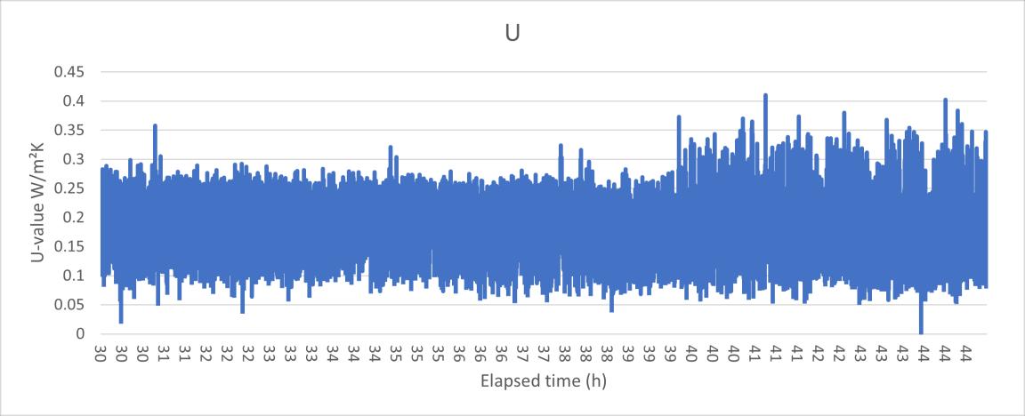
Figure E 2 heat flux data 1
Figure E 3 surface temperature data 1
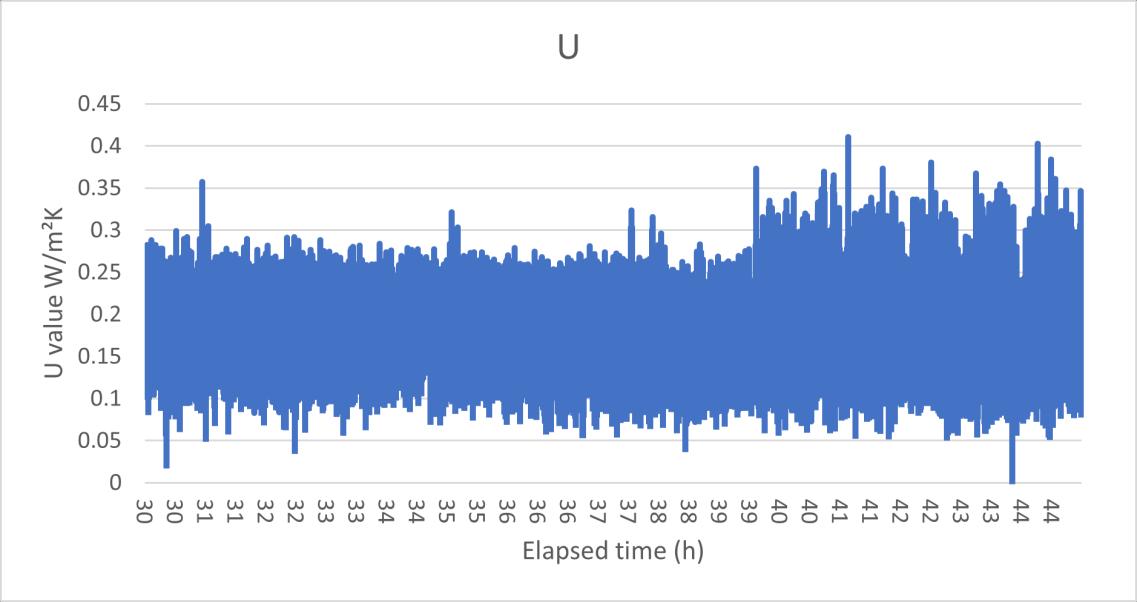
HFM test 2
Name U average when air temperature +/ 1K standard deviation
standard deviation/ average
Uncertainty calculation theory
U2.1 0.183626 0.039499 21.5104% 0.00276 Heat flux 2.1 5.659272 1.221944 21.6% Surface temperature2.1 30.82321 0.489961 1.6%
Table E 2 HFM test result 2.1
Figure E 4 U value data 2.1
Figure E 5 heat flux data 2.1

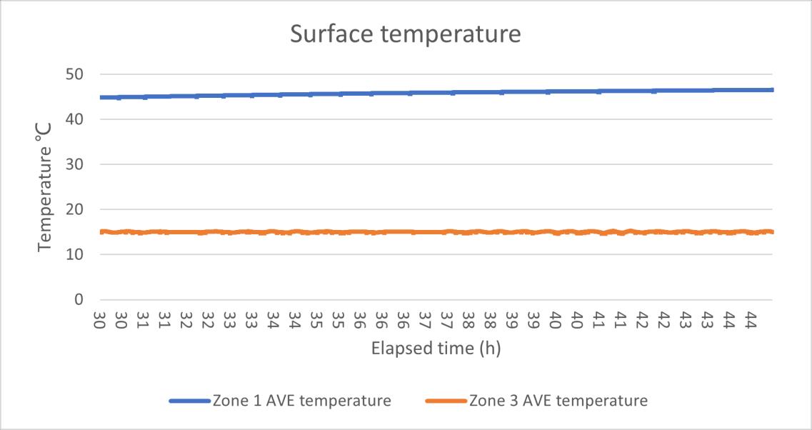
Figure E 6 surface temperature data 2.1
Name U average when air temperature +/ 1K standard deviation
standard deviation/ average
Uncertainty calculation theory U2.2 0.198346 0.042663 21.5096% 0.002982
Heat flux 2 2 5.659272 1.221944 21.6% Surface temperature 2.2 28.53596 0.465948 1.6%
Table E 3 HFM test result 2.2
Figure E 7 U value data 2.2
Figure E 8 heat flux data 2.2
Figure E 9 surface temperature data 2.2
HFM test 3
First one is calculating when air temperature reach sp, second one is calculating when surface temperature reach stable.
Name U average when air temperature +/ 1K standard deviation
standard deviation/ average
Uncertainty calculation theory
U3.1 0.247614 0.08185 33.1% 0.003743 Heat flux 3.1 4.720694 1.257511 26.6% Surface temperature 3.1 19.27699 1.325219 6.9%
Table E 4 HFM test result 3.1
Figure E 10 U value data 3.1
Figure E 11 heat flux data 3.1
Figure E 12 surface temperature data 3.1
Name U average when air temperature +/ 1K standard deviation
standard deviation/ average
Uncertainty calculation theory
U3.2 0.23396 0.044794 19.1% 0.003533 Heat flux 3.2 4.706921 0.898882 19.1% Surface temperature 3.2 20.12297 0.305265 1.5%
Table E 5 HFM test result 3.2
Figure E 13 U value data 3.2
Figure E 14 heat flux data 3.2
Figure E 15 surface temperature data 3.2
HFM test 4
First one has SP 40 in warm side, second one has SP 50 in warm side.
Name U average when air temperature +/ 1K standard deviation
standard deviation/ average
Uncertainty calculation theory
U4.40 0.233591 0.044693 0.19133 0.00352
Heatflux4.40 4.648281 0.891798 19.2% Surface temperature 19.89944 0.270155 1.4%
4.40
Table E 6 HFM test result 4.40
Figure E 16 U value data 4.40
Figure E 17 heat flux data 4.40
Figure E 18 surface temperature data 4.40
Name U average when air temperature +/ 1K standard deviation
standard deviation/ average
Uncertainty calculation theory
U4.50 0.227686 0.036954 16.2% 0.003812 Heatflux4.50 6.521391 1.058262 16.2% Surface temperature
4.50 28.64249 0.142016 0.5%
Table E 7 HFM test result 4.50
Figure E 19 U value data 4.50
Figure E 20 surface temperature data 4.50
Figure E 21 heat flux data 4.50
HFM test 5
With thermal paste and hard tape cover on the heat flux
Name U average when air temperature +/ 1K standard deviation
standard deviation/ average
Uncertainty calculation theory U 0.21418 0.03683 17% 0.003235 Heatflux 4.231742 0.726755 17.2% Surface temperature 19.76048 0.277792 1.4%
Table E 8 HFM test result 5
Figure E 22 U value data 5
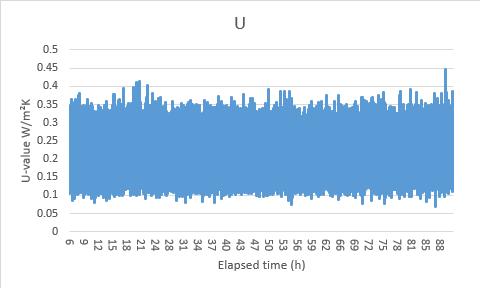
Figure E 23 heat flux data 5
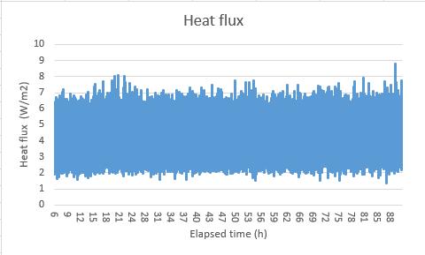
Figure E 24 surface temperature data 5
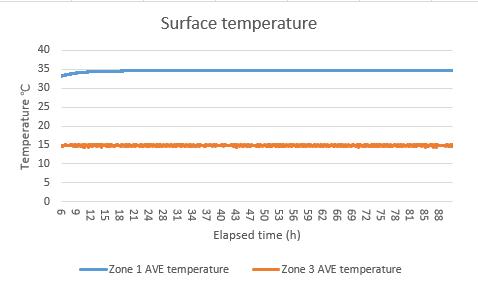
HFM test 6
Paper fabric between the heater/cooler, first one sp 40 in warm side, second sp 50 in warm side
Name U average when air temperature +/ 1K standard deviation
standard deviation/ average
Uncertainty calculation theory
U6.40 0.154173 0.040303 26.1% 0.002319 Heatflux6.40 3.87656 1.013199 26.1% Surface temperature6.40 25.14518 0.188866 0.8%
Table E 9 HFM test result 6.40
Figure E 25 U value data 6.40
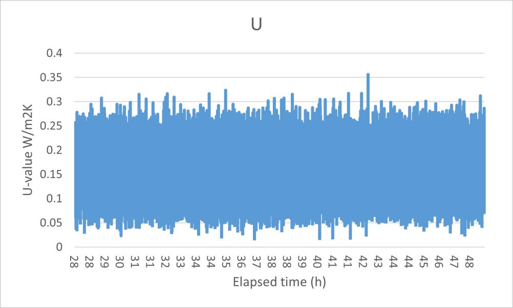
Figure E 26 heat flux data 6.40
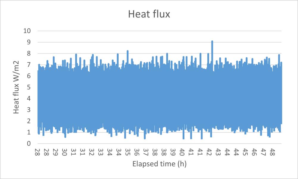
Figure E 27 surface temperature data 6.40
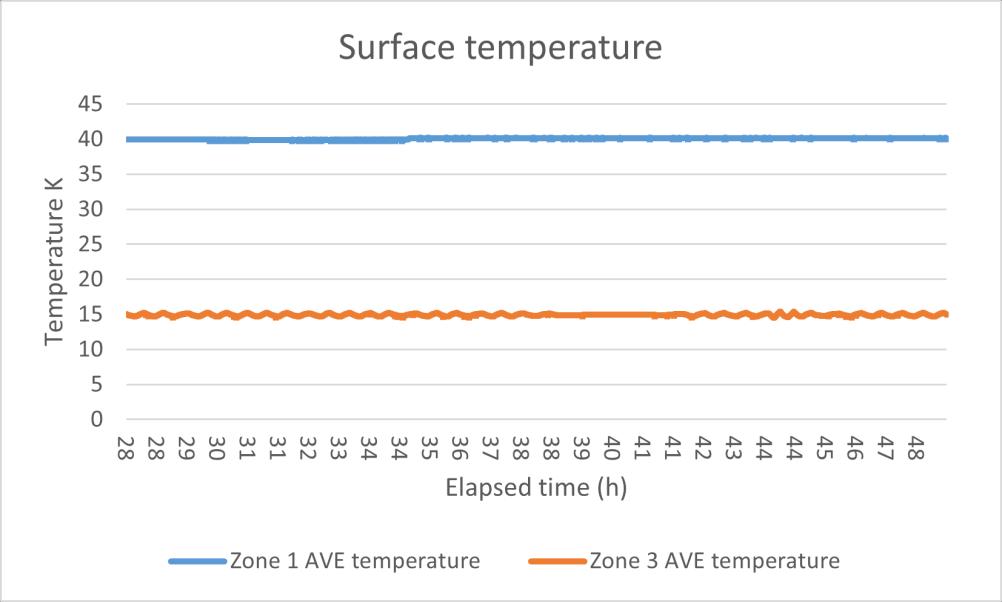
Name U average when air temperature +/ 1K standard deviation
standard deviation/ average
Uncertainty calculation theory U6.50 0.209253 0.02959 14.1% 0.003137 Heatflux6.50 7.327503 1.036834 14.1% Surface temperature6. 50 35.08728 0.13947 0.40%
Table E 10 HFM test result 6.50
Figure E 28 U value data 6.50
Figure E 29 heat flux data 6.50
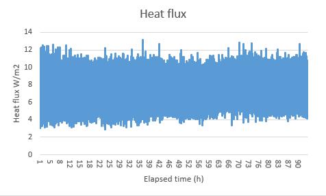
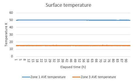
Figure E 30 surface temperature data 6.50
HFM test 7
Heat flux in cold side (cooler off)
Name U average when air temperature +/ 1K standard deviation
standard deviation/ average
Uncertainty calculation theory U 0.073702 0.022829 31.0% 0.001228 Heatflux 1.76071 0.546589 31.0% Surface temperature 23.88362 0.072774 0.3%
Table E 11 HFM test result 7
The elapsed time unit is min. in the figures below.
Figure E 31 U value data 7
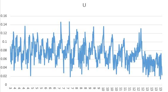
Figure E 32 heat flux data 7
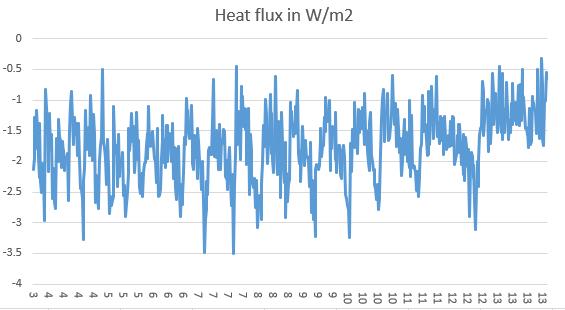
Figure E 33 surface temperature data 7
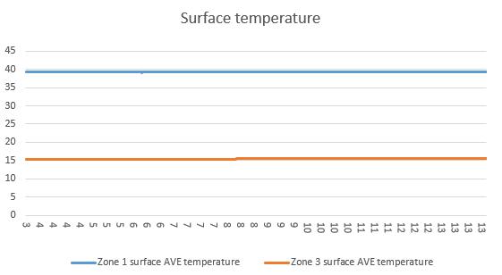
Figure E 34 overall heat flux condition after turned off the cooler in 1h 7
HFM test 8
Heat flux in warm side (heater off)
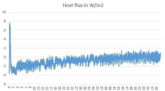
Name U average when air temperature +/ 1K standard deviation
standard deviation/ average
Uncertainty calculation theory
U 0.086368 0.024626 28.5% 0.009991 Heatflux 1.995087 0.568489 28.5%
Surface temperature 23.10169 0.04092 0.2%
Table E 12 HFM test result 8
Figure E 35 U value data HFM 8
Figure E 36 heat flux data 8
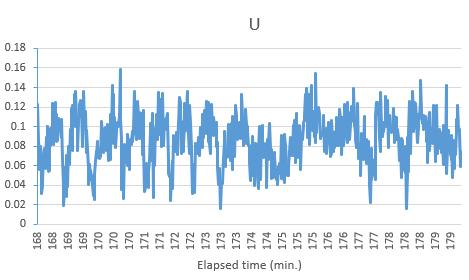
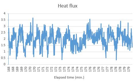
Figure E 37 surface temperature data 8
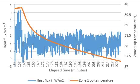
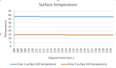
Figure E 38 The overall situation when turn off the heater 8
Other tests
Other test 1
The cover dropped during the test Name U average when air temperature +/ 1K standard deviation
Uncertainty calculation theory U 0.084525 0.053088 62.8078% 0.00172 Heatflux 2.129258 1.122417 52.7140% Surface temperature 18.7684 0.47528 2.5323% Table E 13 HFM test result OT1
standard deviation/ average
Figure E 39 heat flux data OT1
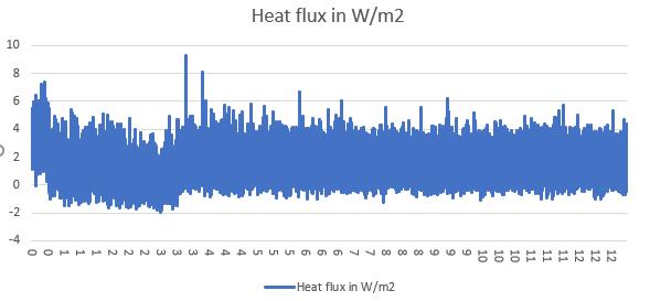
Figure E 40 U value data OT1
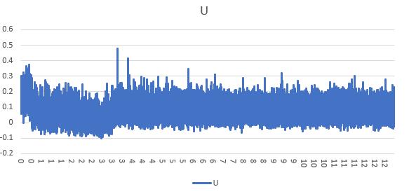
Figure E 41 surface temperature data OT1
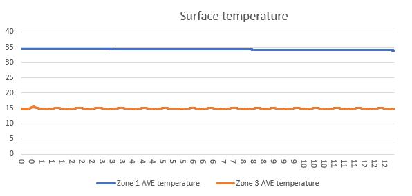
Other test 2
The heat flux sensor in cold side, standard HFM Name U average when air temperature +/ 1K standard deviation
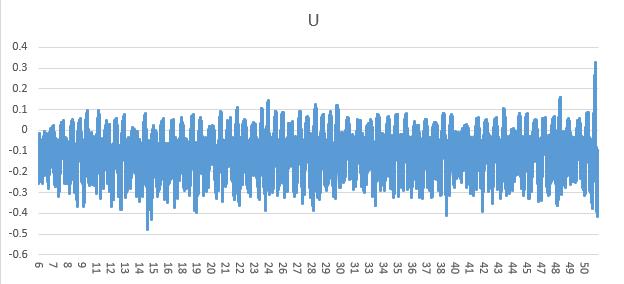
standard deviation/ average
Uncertainty calculation theory
U 0.084525 0.053088 62.8078% 0.00172 Heatflux 2.129258 1.122417 52.7140% Surface temperature 18.7684 0.47528 2.5323%
Table E 14 HFM test result OT1
Figure E 42 U value data OT2
Figure E 43 heat flux data OT2
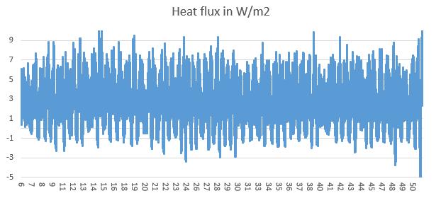
Figure E 44 surface temperature data OT2
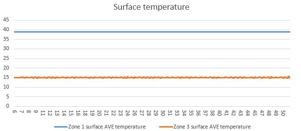
Figure E 45 overall heat flux data OT2
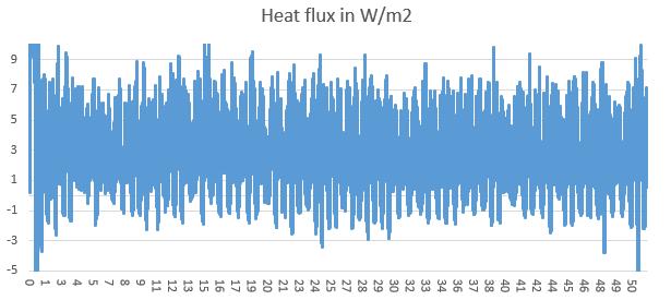
Appendix F- IR tests results
IR test 1
Time
Warm zone IR ColdzoneIR
Temperature difference Heat flux average U(ir)
14:20 38.2589 15.56335 22.69555 3.484086901 0.15
14:30 38.4585 16.0986 22.3599 3.376576675 0.15
14:40 38.6581 15.56335 23.09475 2.584475502 0.11
14:50 38.6581 15.56335 23.09475 2.014634579 0.09
Table F 1 detail IR test 1 data
Name averagevalue standarddeviation uncertainty/average
U 0.126 0.032 25.46%
Temperature difference 22.811 0.355 1.56% Heat flux 2.865 0.694 24.24%
Table F 2 IR test 1result
Figure F 1 IR test 1 surface temperature data
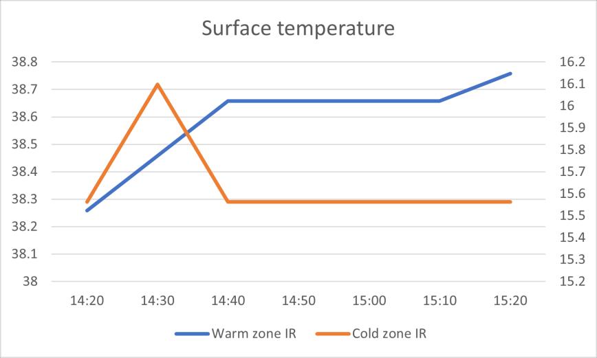
Figure F 2 IR test 1 compare data heat flux and U value
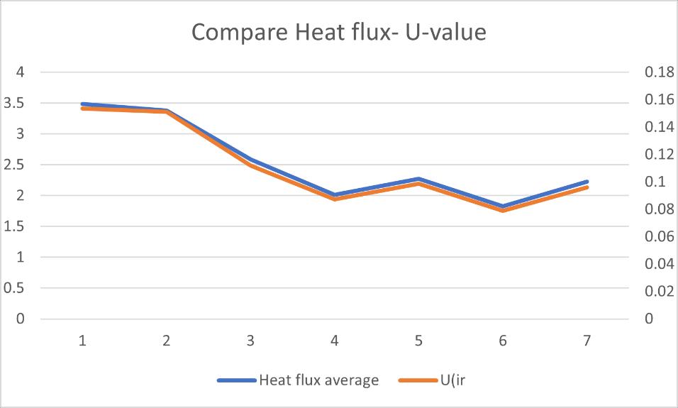
IR test 2
Time Warm zone IR ColdzoneIR Temperature difference Heat flux average U(ir)
13:50 36.3627 21.4511 14.9116 3.671254 0.25
14:00 39.6561 21.4511 18.205 3.814784 0.21
14:10 39.8557 21.98635 17.86935 3.801238 0.21 14:20 40.1551 21.98635 18.16875 3.350947 0.18
Table F 3 detail IR test 2 data
Name averagevalue standarddeviation uncertainty/average U 0.21 0.03 11.9% Temperature difference 17.29 1.59 9.2% Heat flux 3.66 0.22 5.9%
Table F 4 IR test 2 result
Figure F 3 IR test 2 compare data heat flux and U value
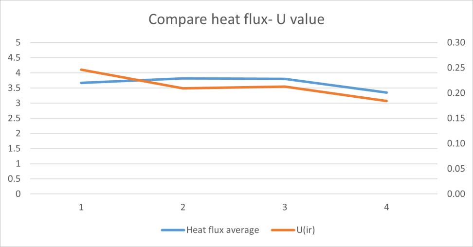
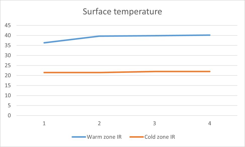
Figure F 4 IR test 2 surface temperature data
IR
test 3
Time Warm zone IR ColdzoneIR Temperature difference Heat flux average U(ir)
13:50 42.6501 21.98635 20.66375 4.54382 0.22
14:00 42.7499 21.98635 20.76355 5.066733 0.24
14:10 42.9495 21.98635 20.96315 4.584503 0.22
14:20 43.0493 21.98635 21.06295 4.883306 0.23
Table F 5 detail IR test 3 data
Name averagevalue standarddeviation uncertainty/average U 0.23 0.01 5.2% Temperature difference 20.86 0.18 0.9%
Heat flux 4.77 0.25 5.2%
Table F 6 IR test 3 result
Figure F 5 IR test 3 compare data heat flux and U value
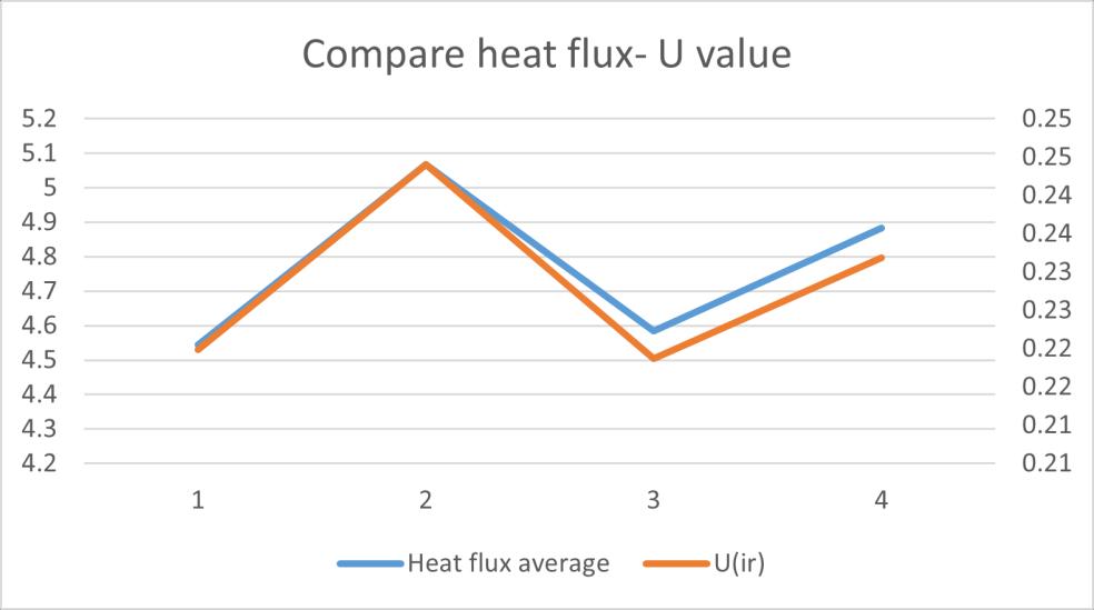
Figure F 6 IR test 3 surface temperature data
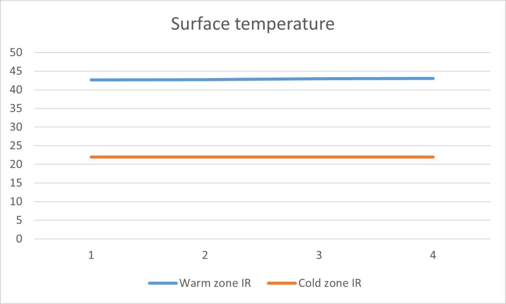
Appendix G- dynamic tests result
Dynamic test 1
Figure G 1 input data dynamic 1
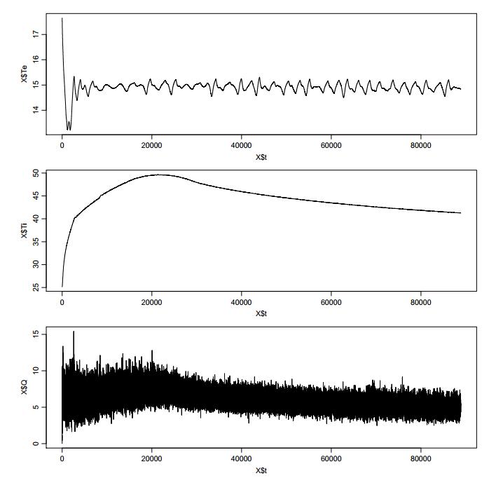
Figure G 2 simulate parameter value dynamic 1
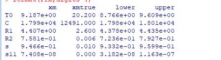
Figure G 3 simulate value compare with real value dynamic 1
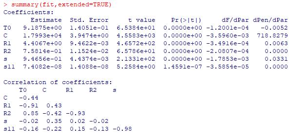
Figure G 4 ACF residuals dynamic 1
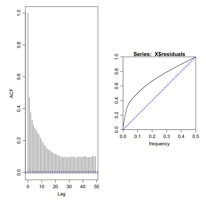
Figure G 5 final result with estimate heat flux dynamic 1
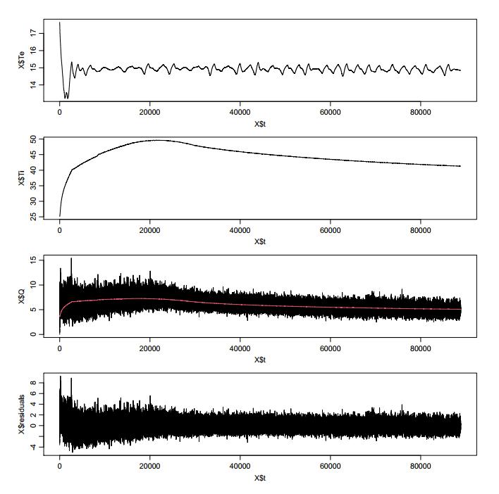
The dynamic test 2
Figure G 6 input data dynamic 2
Figure G 7 simulate parameter value dynamic 2
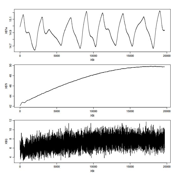
Figure G 8 simulate value compare with real value dynamic 2
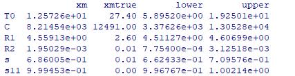
Figure G 9 ACF residuals dynamic 2
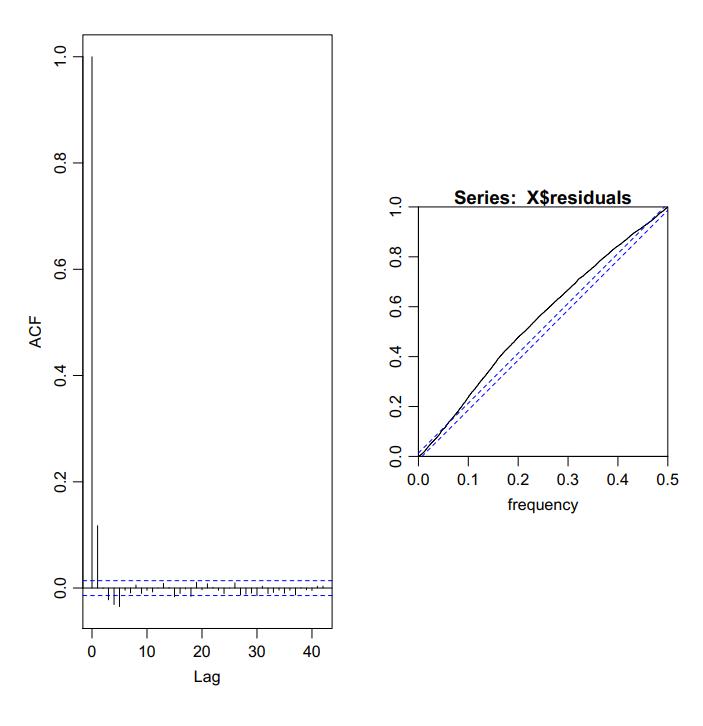
Figure G 10 final result with estimate heat flux dynamic 2
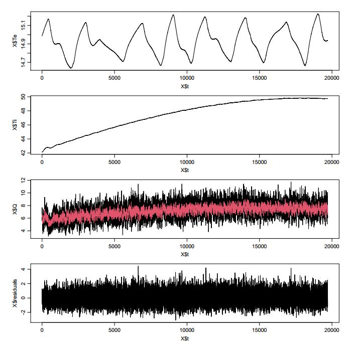
The dynamic test 3
Figure G 11 input data dynamic 3
Figure G 12 simulate parameter value dynamic 3
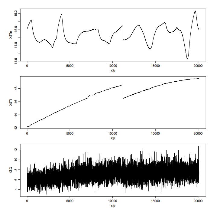
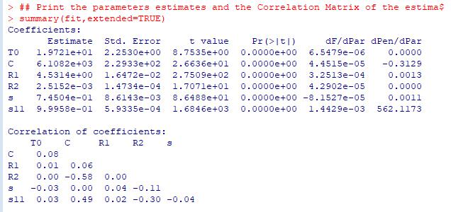
Figure G 13 simulate value compare with real value dynamic 3
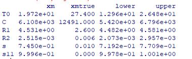
Figure G 14 ACF residuals dynamic 3
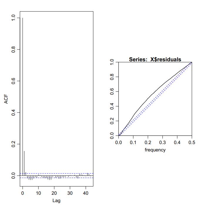
Figure G 15 final result with estimate heat flux dynamic 3
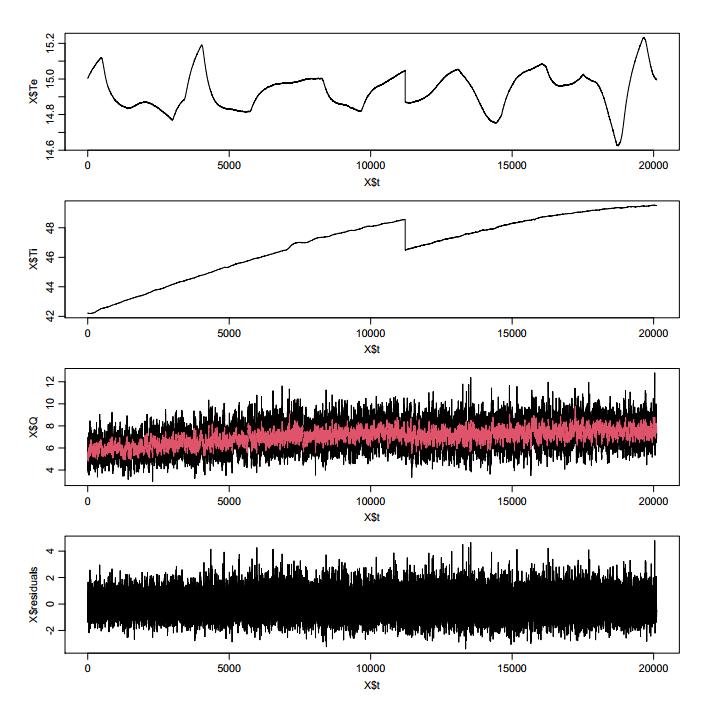
Appendix H- photos from thermography camera
Since the camera has no way to adjust the focus, only a part of the sample wall can be photographed at a time
Figure H 1 IR camera photo 1: HFM
Figure H 2 IR camera photo 1: reference photo
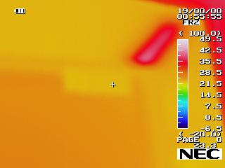
 Figure H 3 IR camera photo 2: corner
Figure H 4 IR camera photo 2: reference
Figure H 3 IR camera photo 2: corner
Figure H 4 IR camera photo 2: reference
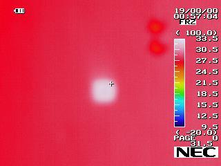
 Figure H 5 IR camera photo 3: fixture
Figure H 6 IR camera photo 3: reference
Figure H 5 IR camera photo 3: fixture
Figure H 6 IR camera photo 3: reference
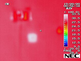
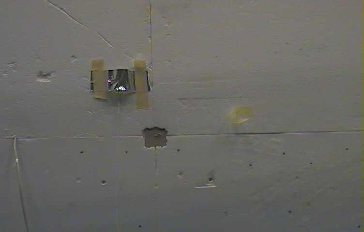 Figure H 7 IR camera photo 4: fixture and heat flux sensor
Figure H 8 IR camera photo 4: reference
Figure H 7 IR camera photo 4: fixture and heat flux sensor
Figure H 8 IR camera photo 4: reference
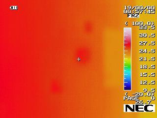
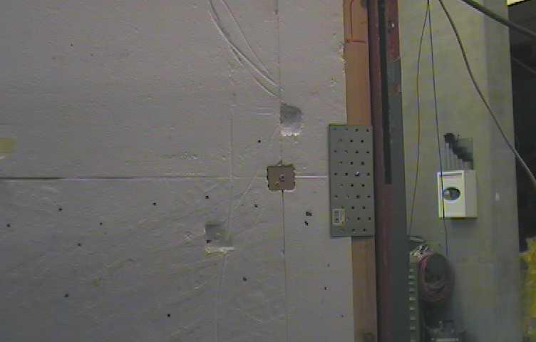 Figure H 9 IR camera photo 5: right side corner and fixture
Figure H 10 IR camera photo 5: reference
Figure H 9 IR camera photo 5: right side corner and fixture
Figure H 10 IR camera photo 5: reference


