Mallari, J. Masigan, J.W. Edaño, Q.A. Uy, M.A. Bautista, C.J. Jasmin, D. Abdao, R.A. Parr, K. Suetos
O. Coroza, N.A. Mallari, K. Andaya, R. Felisimo-Inovejas, D. Darapiza, J. Clemente, N. Chavez, C. Realo, J. Masigan, J.W. Edaño, Q.A. Uy, M.

Mallari, J. Masigan, J.W. Edaño, Q.A. Uy, M.A. Bautista, C.J. Jasmin, D. Abdao, R.A. Parr, K. Suetos
O. Coroza, N.A. Mallari, K. Andaya, R. Felisimo-Inovejas, D. Darapiza, J. Clemente, N. Chavez, C. Realo, J. Masigan, J.W. Edaño, Q.A. Uy, M.


1. Assessing Sukat 1, 2, and 3 begins with a thorough desktop review. You need to gather relevant data and information on species, ecosystems, and habitats present in the area of interest. From this, a separate checklist of species, and ecosystems can be produced. The lists should indicate the species present and their respective habitat types, conservation status, and endemism; the habitat/ ecosystem types present, and their descriptions. These checklists serve as outputs that will justify the presence of Sukat 1, 2, and 3 at the lowest level (i.e. Bronze level).
2. Additional data (e.g. species geographic coordinates) and information (e.g. locality, time of observation) can be sourced from online databases, biodiversity assessment and monitoring reports, and existing publications. With sufficient data and information, area of occupancy (AOO) and extent of occurrence (EOO) maps of a species can be generated. A map (e.g. dot map) of the ecosystem/habitat type present in the area can also be produced. These maps will justify the presence of Sukat 1, 2, and 3 at the Silver level.
3. After gathering data and information from secondary sources, field surveys (flora and fauna assessment, and habitat assessment) will be necessary for ground validation. Data and information collected from field surveys will be used for ecological modeling (e.g. ordination analysis, species distribution modeling) to determine what priority indicator species are present in the area of interest (AOI). Selecting the right species indicators is important for monitoring improved management effectiveness and identifying priority conservation actions. The species distribution models (SDMs) of these selected indicator species will have to be generated to determine species habitat suitability and potential spatial niche. The SDMs allow us to predict how species might respond to changes in their environment, especially in the context of climate change and habitat alteration. The SDMs serve as output for Sukat 1 (Gold level). With sufficient data and information, species population density may be calculated, and results of the analysis will satisfy the highest level of output needed for Sukat 1 (Platinum level). Sukat 1, in general, plays a
crucial role in making informed decisions for conservation and ecological management of rare, threatened, and endemic species.
4. For Sukat 2, a mosaic map of ecosystems will be generated as output for Gold level. Producing this map can only be possible with sufficient data and resources. This requires ground-truthed data for each layer on the map in order to make certain that the presence of the biophysical characteristics depicted by the data layers are correct. This process might involve aerial ground-truthing (e.g. remotely piloted aircraft system) to generate aerial images of the AOI or manual surveys on foot. Apart from the ecosystems map, land cover maps (historical and contemporary) will also be produced. The different land cover classes present in the AOI are to be identified according to the Intergovernmental Panel on Climate Change (IPCC) standards. A final accuracy level between 85% and 90% is accepted for each of the maps of ecosystems (terrestrial), benthic cover (marine), and land cover in order to satisfy the Gold level of standards. These are to be combined later into a mosaic map. A similar process will be done at the Platinum level, except that a multi-layer ecosystem map has to be generated, with a final accuracy within the range of 85% and 90% while an accuracy above 90% is necessary for analyzing Sukat 4. These maps help us understand our existing assets within the landscape or seascape. The results will also feed into the analysis of Sukat 1 (land cover or ecosystems are examples of predictors for SDMs), and Sukat 4, 5 and 6 (extent of ecosystems). Planners, decision-makers, and conservation practitioners rely on these maps to assess risks, prioritize protection efforts, and encourage sustainable land development.
5. The land cover data used for identifying Sukat 2 will be utilized for the analysis and identification of Sukat 3 present in the AOI. However, identifying Sukat 3 will require data from at least two periods (baseline/historical and contemporary) to visualize habitat/ecosystem change and trends. This requires remote sensing methods. Preliminary habitat/ecosystems change analysis will satisfy your Gold level of standard. At the Platinum level, ecosystem change, forest fragmentation, habitat suitability analysis will be required in a mosaic landscape. Identification of presence of threatened ecosystems will be best supported by: (1) hotspot map; (2) ecosystem change; and (3) forest fragmentation analysis overlaid on predicted suitable habitats (SDMs) of indicator species. Determining changes in the condition and extent of ecosystems and land cover enables informed decisionmaking. The results of Sukat 3 are also essential for analyzing Sukat 4, 5, and 6 as these make up the extent
and condition accounts. Policymakers and planners can use this information in mitigating impacts of climate change and anthropogenic activities, sustainable land development, delineating conservation area boundaries, and policy planning.
N.A. Mallari, J. Masigan, J.W. Edaño, Q.A. Uy, M.A. Bautista, C.J. Jasmin, D. Abdao, R.A. Parr, K. Suetos

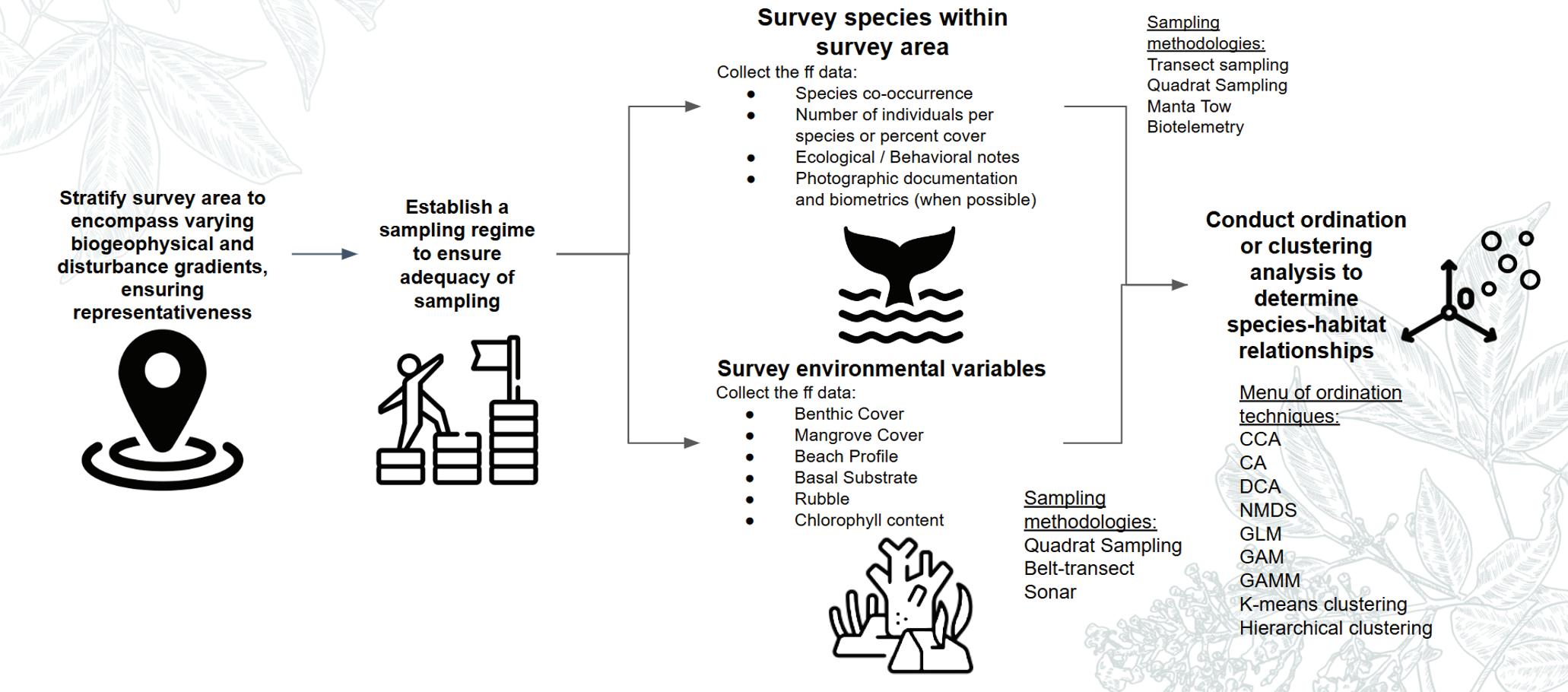
1. When selecting sampling sites, it is important to ensure the representativeness of your survey. This can be done by stratifying the survey area to encompass varying bio geophysical and disturbance gradience. It is also important to ensure the adequacy of sampling, so a sampling regime must be established that is at par with the standard methodologies – one that is appropriate for the specific site.
2. Transect lines, point stations, or sampling plots must be established first. You need to collect both species data and environmental variables. Examples of species data that will be collected are species name, number of individuals, geographic coordinates, observation types, ecological or behavioral notes, and distance from the individual to the transect line or station. Environmental variables may include data on vegetation cover, understory parameters, percent canopy cover, habitat type, and other biophysical parameters. The methodology may be tailored fit as needed, depending on the data that needs to be collected. Here are some references you can use for collecting biodiversity data:
1Including mangrove species surveys
All taxonomic groups1
• Biodiversity Management Bureau and Deutsche Gesellschaft für Internationale Zusammenarbeit (GIZ) GmbH. (2017). Manual on Biodiversity Assessment and Monitoring System for Terrestrial Ecosystems. Manila, Philippines. For Birds
• Gregory, R., Gibbons, D. & Donald, P. (2004). Bird census and survey techniques.
• Bibby, C.J., Burgess, N.D., Hill, D.A., & Mustoe, S.H. (2000). Bird Census Techniques, 2nd ed. Academic Press, London
For amphibians and reptiles
• Bennett, Dl. (1999). Expedition Field Techniques: Reptiles and Amphibians.
• Heyer, W. R., M. A. Donnelly, R. W. McDiarmid, L.A. C. Hayek, & M. S. Foster, editors. (1994). Measuring and Monitoring Biological Diversity: Standard Methods for Amphibians. Smithsonian Institution Press, Washington, D.C.
• McDiarmid, R., M. Foster, C. Guyer, J. W. Gibbons, & N. Chernoff. (2012) Reptile Biodiversity - Standard
Methods for Inventory and Monitoring. University of California Press. Berkeley.
• Simmons, J.E. (2002). Herpetological collecting and collections management. Society for the Study of Amphibians and Reptiles Herpetological Circular 16:1–70.
For mammals
• Barlow, K.E. (1999). Expedition Field Techniques BATS.
• Barnett, A. & Dutton, J. (1997). Expedition Field Techniques for Small Mammals.
• Wilson, D. E., Cole, F. R. Nichols, J. D., Rudran, R. & Foster, M. S. (1996). Measuring and Monitoring Biological Diversity. Standard Methods for Mammals. Smithsonian Institution Press, Washington, D.C.
3. After gathering appropriate and sufficient field data, the species-habitat relationship can be determined through ordination/clustering analysis. The analysis may be done through any of the following statistical techniques: (1) Canonical Correspondence Analysis (CCA); (2) Correspondence Analysis (CA); (3) Detrended Correspondence Analysis (DCA); (4) Non-Metric Multidimensional Scaling (NMDS); (5) Generalized Linear Modeling; (6) Generalized Additive Modeling (GAM); (7) Generalized Additive Mixed Modeling (GAMM); (8) K-means clustering; and (9) Hierarchical Clustering.

Figure 3. Field Surveys for Biodiversity and Habitat Assessment (Continuation)
4. We cannot model suitable habitats or estimate population densities for all the species found within the AOI. Once you have determined the species-habitat relationships from the ordination model, the information generated can be used to select the right indicator species in your AOI. Indicator species provide insights into the health and dynamics of an ecosystem, and the population of other species. They are often sensitive to environmental changes with their presence or absence reflecting the conditions of an ecosystem. Selecting indicator species depends on the specific information needed as different indicators serve different purposes. No single species can tell the complete story of an ecosystem so a combination of species can be selected. Consider various taxonomic groups (birds, plants, amphibians, etc.) to capture different aspects of ecosystem health.
5. Produce a list of selected indicator species and their corresponding species occurrence records. This will later be utilized for species distribution modeling (Gold level).
6. Generating species distribution models2 (SDMs) of your selected indicator species is crucial for PA management as it allows you to predict the location and extent of their suitable habitats. Species distribution modeling can be done using any of the following model algorithms: (1) MaxEnt3; (2) DOMAIN4; (3) BIOMAPPER5; (4) regression-based algorithms; (5) Random Forest6; and (6) Artificial Neural Network7
7. At the Platinum level, the species population density of your indicator species must be generated. This can be done through: (1) Distance sampling8,9; (2) Occupancy modeling10,11; (3) Spot mapping/territory mapping12; (4) Population density based on area of suitable habitats13; (4) Quadrat techniques14; or (5) Mark-recapture techniques15
8. SIBOL has pilot-tested these methodologies in Mt. Mantalingahan Protected Landscape and Seascape, Cleopatra’s Needle Critical Habitat, Puerto Princesa Subterranean River National Park, and Siargao Island Protected Landscape and Seascape. You may access these reports at this link: https://tinyurl.com/SnKsibolsites
2 Read about different models for predicting species distribution:
1. Ramampiandra, E.C, Scheidegger, A., Wydler, J., & Schuwirth, N. (2023). A comparison of machine learning and statistical species distribution models: Quantifying overfitting supports model interpretation. Ecological Modelling, Volume 481, 2023, 110353, ISSN 0304-3800.
2. Elith, J., C. H. Graham, R. P. Anderson, M. Dudik, S. Ferrier, A. Guisan, R. J. Hijmans, et al. (2006). “Novel Methods Improve Prediction of Species’ Distribution from Occurence Data.” Ecography 29: 129–51.
3. Guisan, A., & Zimmermann, N. E. (2000). Predictive habitat distribution models in ecology. Ecological Modelling, 135(2–3), 147–186. https://doi. org/10.1016/S0304-3800(00)00354-9
3 Download the Maxent software and manual here: https://biodiversityinformatics.amnh.org/open_source/maxent/
4 Paper describing the DOMAIN model - Carpenter, G., Gillison, A.N., & Winter, J. (1993). DOMAIN: a flexible modelling procedure for mapping potential distributions of plants and animals. Biodiversity & Conservation, 2(6), 667-680. You can download the paper using this link: https://www.whoi.edu/cms/ files/Carpenter_etal_2003_53463.pdf
5 Check out BIOMAPPER here: https://www2.unil.ch/biomapper/what_is_biomapper.html
6 Valavi, R., J. Elith, J.J. Lahoz-Monfort, & Guillera-Arroita, G. (2021). Modelling species presence-only data with random forests. Ecography, 44: 17311742. https://doi.org/10.1111/ecog.05615
7 Lek, S., & Guégan, J. F. (1999). Artificial neural networks as a tool in ecological modelling, an introduction. Ecological modelling, 120(2): 65-73
8 Buckland, S.T., Anderson, D.R., Burnham, K.P., Laake, J.L., Borchers, D.L. & Thomas, L. (2001). Introduction to Distance Sampling: Estimating Abundance of Biological Populations. Oxford University Press, Oxford, UK.
9 Get the Distance software or Distance R packages, and the Distance sampling manual from this link: https://distancesampling.org/whatisds.html
10Learn more about the concepts behind occupancy modeling from this book - MacKenzie, D. I., Nichols, J. D., Royle, J. A., Pollock, K. H., Bailey, L. L., & Hines, J. E. (2006). Occupancy Estimation and Modeling: Inferring Patterns and Dynamics of Species Occurrence. Elsevier/Academic Press; USGS Publications Warehouse. https://pubs.usgs.gov/publication/5200296
11You can perform occupancy modeling using the PRESENCE software or the RPresence package using the R console. The manuals and documentations on occupancy estimation and modeling are available here: https://www.mbr-pwrc.usgs.gov/software/presence.shtml
12Spot mapping or territorial mapping is usually done for delineating animal territories and estimating the number of breeding territories as an indicator for population size. This technique is most commonly used in bird density studies. Here are some references you can use:
1. Ralph C.J., G.R Geupel, P. Pyle, T.E. Martin, & D.F. Desante. (1993). Handbook of field methods for monitoring landbirds. USDA, Forest Service, General Technical Report PSW-GTR-144. Albany, California, USA.
2. Bibby, C.J., N. D. Burgess, D.A. Hill, & S. Mustoe. (2000). Bird census techniques. Academic Press, London, United Kingdom.
3. Jablonski, K., McNulty, S., & Schlesinger, M. (2010). A Digital Spot-mapping Method for Avian Field Studies. The Wilson Journal of Ornithology. 122. 772-776. 10.2307/40962348.
4. Dorota K., Piotr Skórka, S., & Kazimierz, W. (2019). Delineating the number of animal territories using digital mapping and spatial hierarchical clustering in GIS technology, Ecological Indicators, Volume 107, 2019, 105670, ISSN 1470-160X. https://doi.org/10.1016/j.ecolind.2019.105670
13Sutton, L J., Ibañez, J.C., Salvador, D.I., Taraya, R.L., Opiso, G.S., Senarillos, T.P, & McClure C.J.W. (2023). Priority conservation areas and a global population estimate for the Critically Endangered Philippine Eagle. Animal Conservation. DOI: https://doi.org/10.1111/acv.12854
14 Carah, J., & Chávez, A.M. (2007). Estimating plant population density: Time costs and sampling efficiencies for different sized and shaped quadrats.
15 Different applications of the mark-recapture methods:
1. Milchram, M., Schröder, A., & Bruckner, A. (2020). Estimating population density of insectivorous bats based on stationary acoustic detectors: A case study. Ecology and Evolution, 10(3), 1135-1144. https://doi.org/10.1002/ece3.5928
2. Lettink, M. & Armstrong, D.P. (2003): An introduction to using mark-recapture analysis for monitoring threatened species. Pp. 5ñ32 in Department of Conservation 2003: Using mark-recapture analysis for monitoring threatened species: introduction and case study. Department of Conservation Technical Series 28, 63 p
3. Lebreton, J., Burnham, K.P., Clobert, J., Anderson, & D.R. (1992). Modelling survival and testing biological hypotheses using marked animals: a unified approach with case studies. Ecological Monographs 62(1): 67ñ118.
R.A. Parr, J. Ordinario, B. Hipolito, and A.A. Ramos
1. Proper site selection coupled with a stratified sampling design when sampling marine biodiversity is a vital step in ensuring the adequacy and representativeness of sampling. For example, sampling stations for coral reefs are to be established on upper reef slopes of monsoonfacing reefs as this is the actively growing section of the reef and typically the most representative of hard coral species diversity.
a. Moreover, employing randomization techniques will minimize biases in the data collection process.
b. The recommended stratified sampling design as per the BMB TB 2017-05 consists of (from top to bottom) a set location (e.g., province), wherein several sites are established; each site should have two equally sized replicates or sampling stations; and transects, point stations, and/or quadrat plots to be established within each station.
2. Once locations, sites, and replicates or stations have been established, you must then establish the transect lines, point stations, and quadrat plots depending on the ecosystem type and study objectives. Species data and
environmental variables must be collected, as well as transport data if applicable (i.e. boat speed for manta tow surveys).
a. Examples of species data includes an inventory of species, number of individuals, geographical coordinates, photo documentation, biometrics, and ecological or behavioral notes. The identification of rare, threatened, and/or endemic coral species for Sukat 1 will typically require colony and corallite photos (both with and without scale).
a. Environmental parameters may include vegetation and/or benthic cover, habitat type, water quality, chlorophyll content, and other biophysical parameters.
The methodologies used will depend on the data that needs to be collected. A combination of sampling designs may also be used depending on the marine ecosystem type. For example, seagrass surveys use transect-quadrat and belt transect methods while coral assessments can employ point intercept, belt transect methods, and/or quadrat monitoring. Surveys for large marine vertebrates can also utilize photo
identification, land-based monitoring, interviews, striptransect and line-transect via boat.
Listed below are some references you can use for collecting marine biodiversity data:
• Biodiversity Management Bureau (BMB). Technical Bulletin (TB) 2017-05. Guidelines on the Assessment of Coastal and Marine Ecosystems.
• BMB. TB 2019-04. Annex 1: Assessment and Monitoring Methods for Specific Coastal and Marine Ecosystems.
• BMB and Deutsche Gesellschaft für Internationale Zusammenarbeit (GIZ) GmbH. 2017. Manual on Biodiversity Assessment and Monitoring System for Coastal and Marine Ecosystems. Manila, Philippines.
• Additional references per taxonomic group or habitat.
For Coral reefs*
• Van Woesik, R., Gilner, J., Hooten, AJ. 2009. Standard operating procedures for repeated measures of process and state variables of coral reef environments. Melbourne: Coral Reef Targeted Research and Capacity Building for Management Program, The University of Queensland. 34p.
• Licuanan, W. Y., Mordeno, P. Z. B., & Go, M. V. 2021. C30—A simple, rapid, scientifically valid, and low-cost method for citizen-scientists to monitor coral reefs. Regional Studies in Marine Science, 47, 101961.
For Mollusks
• Bijoy Nandan, Sivasankaran & Jayachandran, P. R. & C V, Asha. 2016. Sampling techniques for molluscan fauna.
For Seaweeds
• Dhargalkar, V. K., & Kavlekar, D. P. 2004. Seaweeds-a field manual.
For Fish
• Cadima, E. L. 2005. Sampling methods applied to fisheries science: a manual (Vol. 434). Food & Agriculture Org.
For Mangroves
• Refer to Sukat 1. Field Survey: Assessing Terrestrial Biodiversity and Habitats.
For Marine Mammals
• Aragones, L. V., Jefferson, T. A., & Marsh, H. (1997). Marine mammal survey techniques applicable in developing countries. Asian Marine Biology, 14(1997), 15-39.
• Alava, M. N., Aquino, M. T., Borja, R., Cruz, R., de Leon, J., Doyola-Solis, E. F., ... & Yaptinchay, A. A. (2014). Philippine Aquatic Wildlife Rescue and Response Manual Series: Marine Turtles.
*Note: Methodologies for assessing coral reef biodiversity can also be incorporated into the development of Sukat 2 and 3 ecosystem maps.
3. After collecting adequate and relevant field data, the species and habitat relationship can be determined through ordination or clustering methods. This analysis can be conducted using various statistical methods, including: (1) Canonical Correspondence Analysis (CCA); (2) Correspondence Analysis (CA); (3) Detrended Correspondence Analysis (DCA); (4) Non-Metric Multidimensional Scaling (NMDS); (5) Generalized Linear Modeling; (6) Generalized Additive Modeling (GAM); (7) Generalized Additive Mixed Modeling (GAMM); (8) K-means clustering; and (9) Hierarchical Clustering.
4. It is impossible to model suitable habitats or estimate population densities for every species within the Area of Interest (AOI). Hence, the information generated from the species-habitat relationships can be used in selecting indicator species as indicator species offer valuable information about the ecosystem and population of other species. It can reflect the changes in the environment, thus allowing us to see problems and changes. It is ideal to include different taxonomic groups (mangroves, seaweeds, mollusks, etc.) to holistically represent the ecosystem health.
5. You may produce a list of selected indicator species and their corresponding species occurrence records. This will later on be utilized for species distribution modeling (Gold level).
6. Indicator species can be used to generate species distribution models (SDMs). This is important because this allows you to predict the distribution of the species with its suitable habitat that can be used for spatial conservation planning. The use of SDMs in marine habitats is a new and innovative approach relative to its use in terrestrial habitats. Listed below are commonly used machine learning tools for generating SDMs in marine habitats16:

(1) MaxEnt17; (2) regression-based algorithms (boosted regression trees)18; (3) Random Forest19; and (4) Aquamaps20
7. At the Platinum level, the species population density of your indicator species must be generated. This can be done through: (1) Distance sampling21,22; (2) Occupancy modeling23; (3) mark-recapture techniques24; and (4) calculating population density based on area of suitable habitats.25,26
8. Alternatively, a platinum output can also be achieved for coral and seagrass species by mapping out their extent and condition through ground-truthed or remotely sensed data. This would illustrate how the conservation value of these species is considered not only through the individual species a reef or seagrass bed is composed of but also through a community-based approach that values their habitat and ecosystem-building capabilities. To learn more about the processes involved in creating this output, refer to sections Sukat 2 and 3. Field Survey: Mapping Marine Ecosystems
16Melo-Merino, S.M., Reyes-Bonilla, H., Lira-Noriega, A. (2020). Ecological niche models and species distribution models in marine environments: A literature review and spatial analysis of evidence. Ecological Modelling, 415, 108837–. doi:10.1016/j.ecolmodel.2019.108837
17Wang, L., Kerr, L. A., Record, N. R., Bridger, E., Tupper, B., Mills, K. E., Armstrong, E.M., and Pershing, A. J. (2018). Modeling marine pelagic fish species spatiotemporal distributions utilizing a maximum entropy approach. Fisheries Oceanography, 27(6), 571-586.
18Becker, E. A., Carretta, J. V., Forney, K. A., Barlow, J., Brodie, S., Hoopes, R., Jacox, M.G., Maxwell, S.M., Redfern, J.V., Sisson, N.B., Welch, H., and Hazen, E. L. (2020). Performance evaluation of cetacean species distribution models developed using generalized additive models and boosted regression trees. Ecology and evolution, 10(12), 5759-5784.
19Phillips, N. D., Reid, N., Thys, T., Harrod, C., Payne, N. L., Morgan, C. A., White, H.J., Porter, S., & Houghton, J. D. (2017). Applying species distribution modelling to a data poor, pelagic fish complex: the ocean sunfishes. Journal of biogeography, 44(10), 2176-2187.
20Check out Aquamaps here: https://www.aquamaps.org/
21Buckland, S.T., Anderson, D.R., Burnham, K.P., Laake, J.L., Borchers, D.L. and Thomas, L. 2001. Introduction to Distance Sampling: Estimating Abundance of Biological Populations. Oxford University Press, Oxford, UK.
22Get the Distance software or Distance R packages, and the Distance sampling manual from this link: https://distancesampling.org/whatisds.html
23Coggins, L. G., Bacheler, N. M., and Gwinn, D. C. (2014). Occupancy Models for Monitoring Marine Fish: A Bayesian Hierarchical Approach to Model Imperfect Detection with a Novel Gear Combination. PLoS ONE, 9(9), e108302. doi:10.1371/journal.pone.0108302
24Durban, J. W., Elston, D. A., Ellifrit, D. K., Dickson, E., Hammond, P. S., and Thompson, P. M. (2005). Multisite mark-recapture for cetaceans: Population estimates with Bayesian model averaging. Marine Mammal Science, 21(1), 80-92.
25Forney, K. A., Ferguson, M. C., Becker, E. A., Fiedler, P. C., Redfern, J. V., Barlow, J., Vilchis, I.L., and Ballance, L. T. (2012). Habitat-based spatial models of cetacean density in the eastern Pacific Ocean. Endangered Species Research, 16(2), 113-133.
26Brownscombe, Jacob & Midwood, Jonathan & Cooke, Steven. (2021). Modeling fish habitat: model tuning, fit metrics, and applications. Aquatic Sciences. 83. 10.1007/s00027-021-00797-5.
Sukat 1 (Species)
Actual Field Survey
Output: Species Distribution Modeling (Gold)
Actual Field Survey
Output: Species Population Estimates (Platinum)
Equipment Cost
Php 2,500,000.00
Php 3,500,000.00
ESTIMATED TOTAL COST: Php 3,100,000.00 to Php 4,100,000.00
*Estimated cost is based on a 120,000 ha protected area COST ESTIMATES
Assumptions:
1. Cost estimates are per site.
2. Estimates are based on direct survey costs and equipment costs* (if applicable).
3. No LOEs are included.
4. No software costs are included.
Survey: 2 months Analysis: 1 month
Survey: 3 months Analysis: 1.5 months
O.
Coroza, N.A. Mallari, K. Andaya, R. Felisimo-Inovejas, D. Darapiza, J. Clemente, N. Chavez, C. Realo, J. Masigan, J.W. Edaño, Q.A. Uy, M. Bautista, C.J. Jasmin, D. Abdao, R.A. Parr, K. Suetos
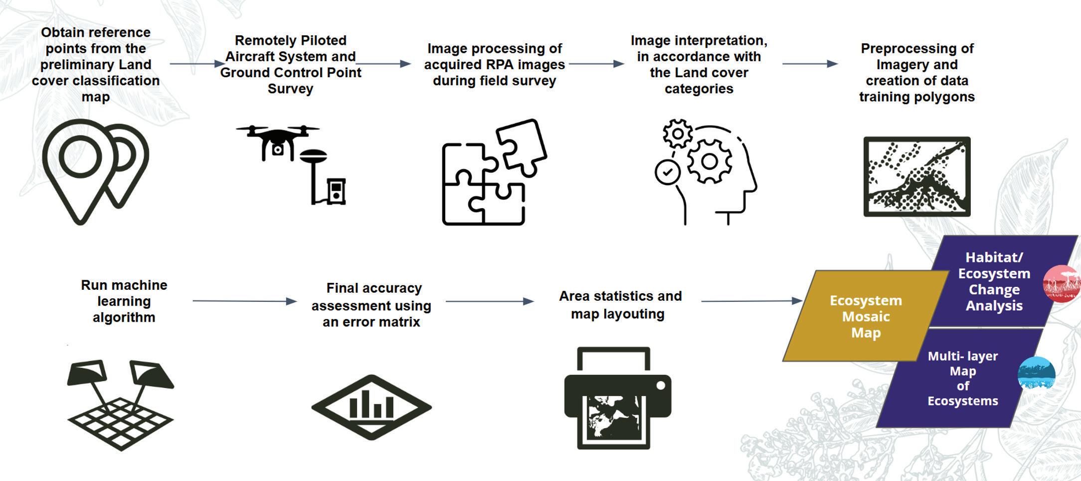
1. Prior to mapping terrestrial ecosystems, you must produce a preliminary ecosystem map of your area of interest (AOI) either based on a secondary source (e.g., Google Earth or land cover maps) or on a primary source either from using the NDVI or clustering methods applied to downloaded Earth observation images (EOIs). You may then assign reference points at random on the preliminary map using any of the mapping software such as QGIS or ArcGIS. Later, you will use these reference points as a guide for the ground-truthing surveys. It is important that the EOIs are either less or free of clouds because they will be obstructions to your view of the land. Pending the establishment of the method for terrestrial ecosystem mapping, you may use proxy land cover classes to map the ecosystem assets.
2. After obtaining the reference points from the preliminary ecosystem or land cover map, you need to assess whether those points fall on land cover classes, which can be identified easily or are indistinguishable from satellite imagery or from Google Earth images. Indistinguishable ones are retained and form part of the points on the ground
that you should visit during the ground-truthing surveys for your next step.
3. The randomly placed reference points with indistinguishable land cover will be the basis for the ground-truthing survey, which you may perform either by using a remotely piloted aircraft system (RPAS) or a manual survey done on foot.
4. The RPAS or drone survey generates multiple photos, which will then be processed and stitched into orthomosaic images.
5. The next step is an aerial photo interpretation or translation of manually obtained field data in accordance with the land cover categories. Your trained observers, either foresters, botanists, or geospatial specialists, will be the ones to interpret land cover categories from the collected data. From there, they will prepare training polygons.
6. From any EOI obtained from step 1 above, you prepare this further with calculated indices to form part of the image
stack for processing through a classification step with a machine learning algorithm.
7. Next, you run your machine learning algorithms through image classification software. So, this is usually done with remote sensing such as SNAP, ArcGIS Pro, QGIS plug-in, Google Earth Engine, Earth Blox, or statistical software like R.
8. Your last step is assessing the accuracy of your results by comparing them with a reference map and establishing an error matrix. Then you can now create and layout your map with the corresponding area statistics of the land cover classes mapped.
O. Coroza, N.A. Mallari, J. Clemente, K. Andaya, S. Claro, J. Masigan, J.W. Edaño, R.A. Parr, Q.A. Uy, M. Bautista, D. Abdao

1. First, you need to collect preliminary data on benthic cover. This is done by obtaining earth observation images of our area of interest from Landsat 8, Sentinel 2, and other repositories of benthic maps. Pending the establishment of the method for marine ecosystem mapping, you may use proxy benthic cover classes to map the ecosystem assets.
2. For creating an ecosystem change analysis map, which is your platinum standard under Sukat 3, you would need to obtain images from two (2) time series, at least usually set a decade apart.
3. In the next step, you would need to layout or input random points using any mapping software such as QGIS or ArcGIS. These points will serve as reference points for use as a guide during the ground-truthing or validation survey. However, before embarking on the field survey, you must examine every reference point using the Earth observation images to check if the benthic cover class is distinguishable. If indistinguishable the reference point is not discarded and becomes a target for the ground truthing.
4. The next step would be to collect the ground-truth data, using any of the following such as a side scan sonar,
remotely deployed vehicle, and other tools to get your data, e.g., presence and extent of coral reef and seagrass.
5. After the survey, your skilled observer classifies the collected benthic data for each ground-truth point according to their correct benthic cover categories.
6. From there, create data training polygons from observed data, which will be used to train the machine learning tool from SNAP or any remote sensing software to automatically process the spectral bands and indices of the concerned Earth observation image (EOI) into the identified classes of benthic cover.
7. An important next step would be to assess the final accuracy of the classified EOI using any of the accuracy assessment tools available in SNAP, ArcGIS, or QGIS plugin. You can do this and produce an error matrix so that you can check how reliable your classified results are compared to a reference map.
8. Lastly, that is when you can create and layout your map and obtain the very important area statistics.
A. Javier, L. Empillo, R. Batistin, C. Suazo, R.A. Parr, N.A. Mallari

1. Gather the best available information available in a site, including land cover or ecosystem maps preferably between two time periods.
2. Do a visual check of the land cover maps to see any potential changes.
3. Place reference points randomly using any GIS software within the chosen AOI. Some reference points can be purposively identified.
4. Ground truthing should be conducted within these reference points to validate the status on the ground. This can be done through manual foot patrols. Collected data should include photo documentation of threats (if applicable), information on drivers of threats, and georeferenced data. From there, one can elucidate the intensity, scope, and frequency of threats.
5. Key informant interviews or focus group discussions can be conducted with relevant agencies or local communities to validate the status of the threats and identify underlying drivers.
6. Finally, threat data should be interpreted and processed relative to the biodiversity and ecosystem data collected. Threats should be mapped out and juxtaposed with land cover data.
SUKAT 2 AND 3. COSTING AND TIMELINE (TERRESTRIAL)
Sukat 2 & 3 (Ecosystems & Habitats)
Terrestrial Ecosystem Mapping (Foot patrols)
3 months Analysis: 3 months Terrestrial Ecosystem Mapping (with Remotely Piloted Aircraft Systems) Php 2,000,000.00
ESTIMATED
*Estimated cost is based on a 120,000 ha protected area
Assumptions:
1. Cost estimates are per site.
2. Estimates are based on direct survey costs and equipment costs* (if applicable).
3. No LOEs are included.
4. No software costs are included.
SUKAT 2 AND 3. COSTING AND TIMELINE (MARINE)
Sukat 2 & 3 (Ecosystems & Habitats)
*Costs do not include satellite images ESTIMATED
*Estimated cost is based on a 26,623 has of shallow marine habitats within a protected area *Costs do not include satellite images
Assumptions:
1. Cost estimates are per site.
2. Estimates are based on direct survey costs and equipment costs* (if applicable).
3. No LOEs are included.
4. No software costs are included.

Ecosystem accounting is organized into two primary procedures: physical accounting which focuses on the quantification of ecosystem extent, condition and creation of physical accounts, and monetary accounting which aims to translate ecosystem services in monetary terms to understand their economic value.
Physical accounting encompasses the systematic evaluation of ecosystem characteristics and begins with the determination of ecosystem extent. This involves collecting data on the size and distribution of ecosystems through methodologies such as benthic and land cover mapping. Continuous or periodic monitoring is emphasized to capture changes in ecosystem types over time. Subsequently, the assessment of ecosystem condition provides insights into the health and vitality of the ecosystems, often conducted through biophysical assessments. Physical accounting ends in tracking of ecosystem service supply and utilization by economic entities, essential for understanding the socioeconomic relevance of ecosystems.
In contrast, monetary accounting involves the conversion of ecosystem services into monetary terms to facilitate economic valuation. This process entails estimating the economic value of ecosystem services using methods such as economic surveys and modeling. These monetary accounts are then integrated into asset accounts, allowing for the analysis of changes in ecosystem value over time that are influenced by factors such as enhancement, degradation, and conversion.
This report underscores the significance of ecosystem accounting in informing evidence-based decisionmaking and policy formulation regarding natural resource management. And by providing a structured approach, that is faithfully based on the UN SEE EA framework, to assessing both the physical and economic dimensions of ecosystems, stakeholders can effectively prioritize conservation efforts and sustainable utilization practices
R.D. Dizon, F. Palermo, R.M. Rosales

SEE EA defines extent accounts, particularly ecosystem extent, as accounts that organize data on the size and extent of ecosystem types that facilitate in the derivation of indicators pertinent to characteristics and the changes that occur within the ecosystem types. It serves as the initial step in ecosystem accounting since it underpins the structure of other accounts. By understanding the size and location of the ecosystem, measurement of ecosystem condition and valuation of ecosystem services become easier to derive.
1. In the context of SIBOL, the process of establishing extent accounts begins with benthic and land cover maps derived from mapping exercises conducted at the sites. These maps, presented in raster format, undergo GIS preprocessing before the actual area computation.
2. The pre-processing involves two key steps: a) Standardizing benthic/land cover classes using the Reclassify by table tool to avoid blunders in succeeding analyses, and b) Utilizing the Polygonize tool to convert the raster image to a vector format.
3. The aforementioned processes allow for the determination of the opening and closing stocks of the sites. However, stopping at this stage would leave us unaware of the changes in cover classes from the opening stock to the end of the closing year. Hence, the Union tool should be employed to generate a cover change vector.
4. From this output, the hectare measurements of each cover change class are computed and presented in a cover change matrix.

1. To assess the condition of the forest ecosystem, the Forest Resources Assessment (FRA) can be done. FRA is a process that collects, manages, makes available and analyzes information on forest resources, their management and uses. It was conducted nationwide through a grant agreement between the Government of the Philippines, through the Department of Environment and Natural Resources (DENR), and the Food and Agriculture Organization of the United Nations (FAO).
2. As for the design of the FRA, Nested Plot Level 1 (rectangular plot measuring 10m x 20m) and Nested Plot Level 2 (circular plot with a radius of 3.99m) are established. The center of the nested plots is located along the plot axis at 5m, 125m and 245m from the plot starting point, respectively.
a. In NPL1 (rectangular plot), saplings (small diameter trees with dbh 10 cm – 19 cm) are measured and recorded.
b. In NPL2, data on edaphic variables and tree regenerations (≥1.3m in height and < 10cm dbh) and other NTFP are collected and recorded
3. FRA makes use of a systematic sampling design, without stratification wherein tracts were established at each 15’ longitude and 15’ latitude and are approximately 25 km apart.
4. Basic forestry information can be collected and monitored through FRA such as diameter at breast height (DBH), total height, merchantable height, species richness, tree cover, and health of trees, among others.

1. The water quality assessment and monitoring activities being done in the protected areas (PAs) through the Biodiversity Assessment and Monitoring System (BAMS) are consistent with the DAO 2016-08 or the Water Quality Guidelines and General Effluent Standards of 2016.
2. Water samples that are being collected in water bodies within the PAs and are subjected to laboratory tests for the following water quality parameters: pH, temperature, dissolved oxygen (DO), total suspended solids (TSS), fecal coliform, phosphate, nitrate, and true color.
3. By monitoring these parameters over time, the water quality condition accounts tables can be developed. These tables will inform if the water quality of the water bodies is declining or are improving.
BMB-DENR
1. The coral reef assessment, facilitated through the Biodiversity Assessment and Monitoring System (BAMS), commences with the layouting of transect lines and quadrats across designated coral reef sampling areas. These areas are then assessed utilizing the photo transect method.
2. Upon completion of data collection, photographs undergo processing and analysis using Coral Point Count with Excel extension software.
3. The generated data are then utilized to construct a coral reef condition accounts table, capturing opening, and closing values gleaned from the assessments.
29PAMO. (2023). Water Quality Monitoring Report.
30PAMO. (2023). Habitat Monitoring Report.
The coral reef assessment conducted by ZSL adheres to a similar procedure as in BAMS. In the development of the coral reef condition account based on ZSL’s Assessment, opening, and closing values of percent cover and reef fish biomass are also recorded. You may access ZSL’s report at this link: https://tinyurl.com/ZSLReport
SEAGRASS BED ASSESSMENT: BMB-DENR
1. The seagrass bed assessment, facilitated through BAMS, begins with laying out transect lines and quadrats across sampling areas. Assessment is typically conducted using the photo transect method, with resulting photos utilized for processing and analysis.
2. Percent cover of the seagrass bed is included in the assessment which is used in the development of a condition account table for seagrass. This table captures data over two periods, encompassing opening and closing values.
MANGROVE FOREST ASSESSMENT: BMB-DENR

1. The mangrove forest assessment, conducted through BAMS, begins with laying out transect lines and quadrats across mangrove sampling areas.
2. Outputs from the assessment, including percent crown cover, average height, and regeneration, comprise the condition account table for the mangrove forest. This table captures data for both opening and closing periods, providing a comprehensive overview of mangrove health and condition over time.
31ZSL. (2021). Resource Assessment of Coastal and Marine Habitats and Recommendations to Improve Management. Philippines Sustainable Interventions for Biodiversity, Oceans, and Landscapes (SIBOL).

1. The mangrove assessment conducted by ZSL follows similar procedures as in BAMS, including the layouting of transects and quadrats over mangrove sampling areas. Assessment of the mangroves adheres to the criteria and guidelines outlined by Primavera et al. in 2014. You may access ZSL’s mangrove assessment report at this link: https://tinyurl.com/ZSLReport
2. Output from the assessment, such as mangrove density, diversity index, and species composition, is employed to develop a mangrove condition accounts table. This table encompasses values from both the opening and closing periods, offering insights into the health and condition of the mangrove ecosystem over time.
32
SUKAT 4. SERBISYONG NAGPAPANATILI NG BUHAY (REGULATION AND MAINTENANCE SERVICES)
Sukat 4.1. Global Climate Regulation Service
G. Castillo, R.M. Rosales, F. Palermo, R.D. Dizon, P.G. David, V.J. Dionisio, & E. Angeles

1. One of the methods in developing carbon accounts is through the use of a land cover change matrix. The land cover change matrix can be done by the “Union” geoprocessing tool in QGIS or ArcGIS. This tool requires two vectorized land cover maps (shapefiles) of different years wherein the Input layer is the opening year, and the Overlay layer is the closing year. The output of this process is the land cover change map.
2. After exporting the attribute table of the land cover change map into a spreadsheet (.csv), the land asset accounts table can now be developed. This table will tell us the changes (additions and reductions) in area for each land cover type.
3. This land asset accounts table can be transformed into timber accounts by converting the area (in hectares) into tree volume (in cu.m) by land cover using conversion factors.
4. The resulting timber accounts table can be used to estimate the biomass content (in tons dry matter/tdm) for both above and below ground. The estimated biomass can now be converted into its carbon content (tC) and ultimately to carbon dioxide equivalent estimates (tCO2e).
5. The social cost of carbon (SCC) is being used to estimate the damage cost avoided for every ton of carbon dioxide released in the atmosphere. Hence, by multiplying the SCC and the computed carbon dioxide equivalent estimates (tCO2e), we can now have the monetary value of the carbon stock and carbon net sequestration/ emission.
Survey: 3.5 months Analysis: 3 months
Assumptions:
1. Cost estimates are per site.
2. Estimates are based on direct survey costs and equipment costs* (if applicable).
3. No LOEs are included.
4. No software costs are included.
T. Balangue, J. Shiraishi, V.J. Dionisio, C. Tee

1. For the Coastal Protection Valuation process flow chart, the first step is to identify the site or sites that will be studied.
2. Following that is the mapping of the chosen study sites. Which consists of the identification and labeling of the coastal communities, mangrove forests, coral reefs, seagrass, seawall, rock boulders, bathymetry, elevation, and foreshore without forest.
3. The third step is to get the historical data on typhoons that affected the site or sites. This can be requested from PAGASA. Alongside this, you may opt to use EMDAT data, which can be requested online through their website.
4. After gathering the historical data on typhoons, the identification of the typhoons’ wind gusts, peak wave height or storm surge height, and year of occurrence, as well as the ranking of the typhoons from highest to lowest peak wave.
5. Step 5 is the identification of the flood-risk zones in the area. This can be accomplished by comparing the area’s elevation to the typhoon’s peak wave or storm surge height.
6. Following this is an actual ground survey, where the following data were gathered: damage cost of the facility, rehabilitation cost (including water and electricity repairs), and lastly the foregone income of the people affected by the typhoon. The mentioned data can be gathered from different economic sectors, such as residential, commercial, institutional, agriculture, fishery, infrastructure, and the tourism sector.
7. After the data gathering, the avoided damage cost was computed using the method where we compared two scenarios: with mangroves and without mangroves. The formula is the Damage cost of a site without mangroves vs. the Damage cost of a site with mangroves.
8. For the next step, you can simulate different potential impacts of different typhoons following steps 3 to 5. If you already have the historical data, you can simulate the potential flood risk zones of the site or sites using the peak wave height or storm surge height of different typhoons.
9. Next is the computation of the Annual Coastal Protection Value of Mangrove under different typhoons. To do so:
a. You must calculate the AER first using the formula Total number of typhoons that affected the site plus 1, and then divide it by their ranking.
b. Next is to calculate for the AEP, 1 DIVIDED BY AER
c. Then you will get the Annual Coastal Protection Value by using the formula:
Storm Surge Height * Probability of Occurrence * Cost Storm Surge Factor
Where,
The cost storm surge factor can be calculated by using the avoided damage cost computed from step 6, and then dividing it by the storm surge height.
10. Then based on your findings, crafting policy recommendations and mitigation/ adaptation measures shall be the final step.
11. The cost storm surge factor can be calculated by using the avoided damage cost computed from step 6, and then dividing it by the storm surge height. 11. SIBOL has pilot-tested these methodologies in Siargao Protected Landscape and Seascape. You may access the report at this link: https://tinyurl.com/coastalprot
Costing and Timeline For Sukat 4.12. Coastal Protection Services
Mapping out of the actual extent of flood and the damaged establishments
Cost and extent of flood data (SIBOL KII survey) and Request of damage reports from LGUs
Assumptions:
1. Cost estimates are per site.
2. Estimates are based on direct survey costs and equipment costs* (if applicable).
3. No LOEs are included.
4. No software costs are included.
1 Month Analysis: 1 Month
Data: 1 Month Analysis: 1 Month
R.M. Rosales, J. Shiraishi, V. Hilomen, J. Fragillano, R. Fragillano, C. Tee, L. Yu, R.D.
SUKAT. 5.5 WILD FISH AND OTHER NATURAL AQUATIC BIOMASS PROVISIONING SERVICES

Figure 20 shows the overview of the methodologies and processes involved in assessing provisioning services for marine ecosystems, specifically focusing on fish provisioning services within the Sukat 5.5. These methodologies have been pilot-tested by SIBOL in Masinloc-Oyon Bay Protected Landscape and Seascape and Siargao Protected Landscape and Seascape. The report is available through this link: https://tinyurl.com/fishprov
The process flow delineates four major steps within the process flow diagram: data gathering, survey outputs, data cleaning and management, and data processing and analysis.
1. The initial step in the process involves training of enumerators who will conduct comprehensive data gathering through surveys. The outputs of these surveys are categorized into two: the Fish Catch Monitoring Gear Inventory (FCMGI) and Enhanced Socio-Economic Assessment and Monitoring (ESEAMS).
2. The next step is data cleaning and database management which is significant for ensuring the accuracy and integrity of collected data.
3. Finally, the processing and analysis of data culminating in valuable insights regarding the supply and use of fish provisioning services within marine ecosystems.
From the diagram, the major steps in ecosystem accounting are highlighted which are the physical and monetary supply and use boxes within the framework. Physical accounts are elucidated through the FCMGI survey. Conversely, monetary accounts are delineated through the ESEAMS survey. You may access the official ESEAMS and FCMGI reports at this link: https:// tinyurl.com/ESEAMSFCMGI
Fish Provisioning Services: Physical Supply & Use

33
4. This process flow diagram highlights the procedures employed in the FCMGI survey. The initial phase of data gathering involves comprehensive training and supervisors who speak the dialect of the site, which ensures the effective execution of surveys and interviews conducted within the targeted communities. During the survey and interview process, two primary surveys which constitute the FCMGI survey were conducted:
a. Fish Gear Inventory (FGI): This survey entails gathering information regarding the fisheries landscape, including aspects such as the number of capture fishers, types of boats and fishing gears utilized, seasonality of gear usage, catch rates, and trends in catch composition over time. The documentation of these parameters provides us insights into the socioeconomic dynamics of fishing communities.
b. Fish Catch Monitoring (FCM): This survey is implemented through a structured 2-day work plus 1-day rest pattern to minimize bias and enhance randomization among intercepted fishers at landing sites. Enumerators recorded data on fishing gear used, fishing effort, location of fishing, volume of catch, species composition, and biometric measurements of intercepted fish, crabs, and squids. This information provides us insights into fishery productivity and species composition.
5. Following data collection, processes such as encoding, unit standardization, and table generation were undertaken to ensure data integrity. One of the first uses of outputs derived from FCMGI is the identification of ecosystem-species associations, particularly species associated with coral reefs, seagrasses, mangroves, and open sea habitats.
Fish Provisioning Services: Monetary Supply & Use

34Rosales, R.M., Shiraishi, J., Tee, C.K. & Yu, L. (2023). Enhanced Socio-Economic Assessment and Monitoring System Technical. Philippines Sustainable Interventions for Biodiversity, Oceans, and Landscapes (SIBOL).
The Enhanced Socio-Economic Assessment and Monitoring System (ESEAMS) survey is a tool utilized by the Department of Environment and Natural Resources (DENR) to evaluate socio-economic conditions within NIPAS Protected Areas. ESEAMS will serve as a primary data source for baseline information on resource use, resource users, and household profiles within PAs.
Formerly utilized through SMART, SIBOL is transitioning to an enhanced and automated version of ESEAMS utilizing ArcGIS Survey 123, hence, the methods delineated in the framework would refer to procedures for using the survey through ArcGIS Survey 123. The transition marks a significant advancement in data collection and management. Unlike previous iterations utilizing SMART, this automated version eliminates the need for manual conversion of raw data to
.csv files and standardization processes. Moreover, the main difference between automation using ArcGIS Survey 123 and SMART lies in the efficiency of data processing.
However, regardless of the automation platform employed, the outputs remain consistent, i.e., comprehensive demographic, economic, and perception data crucial for informed decisionmaking and policy formulation. Key information gathering through the ESEAMS survey encompasses demographics, household income, expenditures, housing, sanitation, health, PA perceptions and knowledge, as well as institutional knowledge and enforcement perceptions. These insights serve as invaluable inputs for designing targeted interventions and management strategies aimed at enhancing socio-economic well-being and conservation outcomes with protected areas.
Costing and Timeline for Sukat 5.5. Wild fish and other natural aquatic biomass provisioning services
Assumptions:
1. Cost estimates are per site.
2. Estimates are based on direct survey costs and equipment costs* (if applicable).
3. No LOEs are included.
4. No software costs are included.
H.A. Francisco, F. Palermo, J.J. Dida, G. Castillo, C.D. Predo, R.M. Rosales, & R.D. Dizon

1. The extent of the almaciga trees can be estimated using the species distribution model (SDM). The results of the SDM tell us which areas are not suitable and which areas have low, moderate, and high suitability for almaciga trees. In the context of NCA for almaciga resin provisioning service, only the areas with a high probability of having almaciga trees are considered. Hence, the SDM maps should be overlayed with the land cover and barangay boundary maps to estimate the highly suitable areas by land cover and by barangay.
2. As for the condition of these ecosystems with almaciga trees, we can assess them in terms of the elevation, distance from the road network, slope, and the state of degradation (i.e., no, low, moderate, and high degradation).
3. In estimating the physical supply of almaciga resin, we can conduct a complete inventory of almaciga trees in the area. This inventory should include the following: geographic coordinates of the trees, DBH, height, and the condition of the trees (i.e., healthy, with diseases, with termites, etc.).
4. If this cannot be done, alternatively, we can use the sampling of almaciga trees which is one of the requirements in applying for resource use permits by almaciga concessionaires. This can be requested from the DENRCENRO. Most of the time, the coordinates of the trees are not being collected. Hence, we can simply randomize the trees in the high SDM areas within the concession area.
5. Both the inventory and concession data can give us an idea of how many almaciga trees are present in the area. Based on the DBH of these trees, we can now estimate the total potential harvestable resin within the PA.
6. To estimate the physical supply and use for almaciga resin, we can use the collected information on the number of tappers in the PA as well as their average annual harvest. These data can be collected through surveys, key informant interviews, and focus group discussions. We can also validate this with the use of the annual allowable harvest that can be collected from the DENR-CENRO. This information can help estimate the volume of almaciga resin that is being harvested within the PA.
7. To estimate the monetary value of almaciga resin provisioning service of the ecosystems, we will need to compute the resource rent. This can be done using the E-SEAMS data which can be validated by the key informant interviews conducted. Finally, the estimated resource rent for almaciga resin harvesting per kilogram is multiplied by the total estimated resin volume harvested to compute the total monetary value of the almaciga provisioning service of the PA.
8. SIBOL has implemented pilot tests of these methodologies in Cleopatra’s Needle Forest Reserve and Puerto Princesa Subterranean River National Park. The reports can be accessed using this link: https://tinyurl.com/ntfpreport
Costing and Timeline for Sukat 5.6. Wild animals, plants, and other biomass provisioning services (NTFP)
Extent, Condition, and Physical Supply Accounts
Monetary Supply
Community mapping, Key Informant, Interviews, and Focus Group Discussion
COSTING AND TIMELINES
Data: 1 Month Analysis: 1 Month Almaciga Inventory
3 Months
1 Month
COSTING AND TIMELINES
Enhanced Socio-Economic Assessment and Monitoring System (E-SEAMS)
ESTIMATED TOTAL COST: Php 1,935,000.00
Assumptions:
1. Cost estimates are per site.
2. Estimates are based on direct survey costs and equipment costs* (if applicable).
3. No LOEs are included.
4. No software costs are included.
3 Months
Castillo, R.M. Rosales, F. Palermo, R.D. Dizon, R. Flores, P.G. David, E. Angeles, & V. Dionisio

One of the most important functions of GIS in hydrology is the delineation of catchments and stream order. This process is vital in water resource management as it helps in the understanding of the distribution and water flow within a watershed. The process flow shown in Figure 24 provides an overview of the stream and catchment delineation using the PCRaster tool in QGIS. PCRaster is a QGIS plugin designed for map algebra and dynamic environmental modeling35. The application of PCRaster lies in environmental modeling disciplines, one of which is hydrology.
1. For the delineation process, a Digital Elevation Model (DEM) file that covers the study area is required as the base input from which all the output rasters will be derived. It is recommended to use a higher resolution DEM, as this provides a more accurate and precise delineation of catchments and stream order, as well as in identifying other geomorphological catchment characteristics. Furthermore, it is crucial that the projection of the DEM is set according to the appropriate plane coordinate grid system of the study area (i.e. UTM Zone 50N) as this is essential for the accuracy and consistency of the spatial analysis of the final output. Once these are all set, the first step in the catchment delineation process can be started.
2. Using the PCRaster Plugin installed in QGIS, the first step is to convert the DEM file into a PCRaster format. It is essential to do this as this enables later processes under the PCRaster tool to be executed.
3. Once converted, the PCRaster version of the DEM is to be used as the input to generate the local drain direction or the flow direction raster. To further improve the styling and visualization of the flow direction, arrows can be added. This can be done by converting the flow direction layer to a mesh through the PCRaster LDD to Grib of the Crayfish plugin, enabling the mesh styling functionality of QGIS where the arrow vectors can be enabled.
4. To generate the stream order raster, the PCRaster Streamorder tool will be used where the flow direction raster will serve as the input local drain direction layer.
5. The next step is to calculate the volume accumulated by the stream. However, this process requires a material layer input. Hence to generate the material layer, the PCRaster Spatial tool will be used where the input nonspatial value should be set to one, the output data type to scalar, and the flow direction raster as the mask layer.
6. Once the material layer is generated, the volume accumulation can be calculated through the PCRaster Accuflux tool. This is where the previously generated material layer will be used alongside the flow direction raster as the LDD input.
7. The next step is to identify the stream order with values greater than or equal to five. However, an input layer as the basis for comparison must be generated first. This can also be done through the PCRaster Spatial tool in which the input nonspatial value is to be set as one, the output data type as ordinal, and the stream order as the mask layer.
8. Once the layer is generated, the identification of stream order with values greater than or equal to five can be executed through the PCRaster Comparison Operators. Under the PCRaster Comparison Operators dialogue box, the stream order raster will serve as the first input with comparison operators being “greater than or equal” (>=), and the input layer previously generated as the last input. The output of this process will be called the river raster with pixel values ranging from zero (0) to one (1) with zero representing non-river stream orders and one as those that are identified as river stream orders.
9. Using the river raster, the river stream order raster can be generated by reflecting stream order pixel values that are greater than or equal to five. This can be done through the PCRaster If Then tool where the river raster will serve as the input and the stream order raster as the true input.
10. To generate the river downstream raster, the PCRaster Downstream tool will be used with the flow direction raster as the flow direction layer and the river stream order raster as the raster layer. The output river downstream raster will serve as an input in generating the junction raster.
11. Generating the junction raster is to be executed using the PCRaster Comparison Operators where river stream order that is not equal to river downstream will become the river junction. The output pixel value ranges from zero (0) to one (1) with one representing the river junctions.
12. Unique ID must be given to the river junctions. To do this, the PCRaster Unique ID tool will be used with the river junction raster as an input. The output is a raster of the river outlet ID. 35PCRaster Tools — QGIS Python Plugins Repository. (2023). Qgis.org. https://plugins.qgis.org/plugins/pcraster_tools/
13. The river outlets ID must be converted to a nominal data type and to do this, the PCRaster Convert Layer Data Type tool must be used with the river outlets ID raster as the input and the output data type as nominal. The output outlets raster will then be used in generating catchment and subcatchment rasters.
14. To generate both rasters, PCRaster Catchment and PCRaster Subcatchment tools are to be used with the flow direction raster as the LDD layer and the outlet raster as the outlet layer.
15. To identify and determine the area of the catchments and subcatchments as well as the length of river stream order per municipality or barangay, the generated catchment, subcatchment, and river stream order rasters must be converted to a vector layer. To do this, the Polygonize (Raster to Vector) should be used with the aforementioned rasters as the input.
16. The output vectors will be intersected each with the vector layer of the municipality or barangay boundary layers. This is to be executed using the Intersection tool where the input layer is the vector layer of the converted rasters, and the municipality or barangay boundary layer as the overlay layer. The output will be an intersection vector.
17. Computation of the catchment and sub-catchment area per municipality or barangay can be done through the field calculator in the attribute table of the intersection vectors. In the field calculator, the output field type must be set to “Decimal Number (Real)” and the input expression should be “area($geometry)”.
18. On the other hand, the same procedure is to be executed in determining the length of the river stream order. However, the input expression in the field calculator must be changed to “$length”.
19. Once calculations for all intersection vectors are done, the information on the attribute table of the vectors can now be exported as a “.csv” file. Data organization and analysis can be executed through the pivot table in Excel.

1. Physical accounting for the water provisioning services makes use of the following inputs: precipitation and humidity, evapotranspiration, digital elevation model (DEM), water abstraction and returns, soil map, land cover map, and discharge data.
a. Water abstraction and returns can be estimated by conducting surveys and key informant interviews. These primary surveys are being done to collect data on the
36WAVES (2016), Bansode and Patil (2016), SEEA (2012)
volume of unmetered and piped water that is being used for drinking, agriculture, and other uses.
b. Through DEM, we can delineate the watershed and sub-watershed boundaries and map out the flow direction, flow accumulation, and stream network.
2. These data are inputs to run the Soil and Water Assessment Tool (SWAT) and Integrated Valuation of Ecosystem Services and Tradeoffs (InVEST) models. These models
are both used to estimate the physical supply of water in the form of the following water balance parameters: precipitation, returns (water flowing back to the streams/ rivers as runoff), evapotranspiration, surface runoff, and water utilization (abstracted water). These parameters are then used to develop the water physical supply and use tables.
3. Part of the accounting work as well is to assess the water users by sector. By conducting surveys, key informant
interviews, and focus group discussions, supported by secondary data, we can estimate the water demand and costs by water users: household/domestic users, farmers/ agricultural users, commercial users, and institutional users. Costs and returns of the water service providers (e.g., water districts, waterworks, local water systems, etc.) in providing drinking water should also be studied as these data are used to compute the resource rent for water supply. The estimated resource rent is used to compute the total monetary value of water provisioning services with the PA.
Costing and Timeline For Sukat 5.7 Water Supply Provisioning Service
ESTIMATED TOTAL COST: Php 500,000.00 TO Php 1,000,000.00 COSTING AND TIMELINES
1. Key Informant Interviews (households, farmers, water service providers, and resort owners)
2. Secondary data gathering (onsite visit of water districts and water users)
3. Geotagging of water sources Php 500,000.00 to Php 1,000,000.00
Assumptions:
1. Cost estimates are per site.
2. Estimates are based on direct survey costs and equipment costs* (if applicable).
3. No LOEs are included.
4. No software costs are included.
Data: 3 months
Analysis: 3 months
SUKAT 6.1 SPIRITUAL/SYMBOLIC SERVICES

The methodology for conducting spiritual valuation begins with the identification of a suitable study site, taking into account accessibility and relevance to indigenous communities. A thorough literature review should be conducted to gather insights into the cultural nuances and spiritual beliefs of the indigenous people inhabiting the selected area. Subsequently, all pertinent information obtained from the literature review is documented, laying the groundwork for the ensuing steps of the study. Focus group discussions (FGDs) are organized and conducted, involving representatives from various segments of the indigenous community, including leaders, healers, men, women, and youth. These participants are to be segmented into groups based on the social structure of the community to ensure diverse perspectives are captured effectively. Through word association exercises, the aim is to unearth the indigenous people’s thoughts and perspectives regarding the connection between the forest and spirituality, as well as their aspirations and significant life aspects. Beads can be employed as a relative ranking tool to highlight the importance of different aspects, starting with dominant spirituality, and then incorporating aspirations. The data collected from these exercises will be encoded for efficient processing and analysis. The next step is to conduct comparative ratio calculations to quantify the spiritual value of the forest per person for each sector, incorporating both qualitative insights and quantitative measures. In instances where indigenous population data is unavailable, an alternative is to derive it from census data, with appropriate exclusions and allocations made based on FGD outcomes. Finally, the total spiritual value of ecosystem services per year is computed by multiplying the indigenous population count per sector by the spiritual value of the forest per sector, encapsulating the holistic essence of spiritual valuation within indigenous communities.
SIBOL has conducted pilot tests of these methodologies in Barangay Ransang, Rizal, Palawan. You can find the report at this link: https://tinyurl.com/spiritualreport
Calculating the Spiritual Value of Ecosystem Services
1. Calculate comparative ratios of beads per sector and spirituality by dividing the total number of beads for each aspect of spirituality.
2. Calculate comparative ratios of beads in terms of spirituality and aspirations by dividing the total number of beads placed on spirituality and aspirations.
3. Compute the monetary value of aspirations using the costmethod technique, considering the total yearly cost of each aspiration per person, obtained from relevant data sources like the Philippine Statistics Authority (PSA).
4. Calculate the total economic value by multiplying the total cost of aspirations divided by the corresponding ratio. Subtract this from the total cost of aspirations to obtain the spiritual value of the forest per person for each sector.
5. If indigenous population data is unavailable, derive it from PSA census data, excluding children aged 0-4 years and allocating individuals to each sector based on FGD outcomes.
6. Compute the spiritual value of ecosystem services by multiplying the indigenous population count per sector by the spiritual value of the forest per sector.
7. Sum up the total spiritual value of ecosystem services per year.
Assumptions:
1. Cost estimates are per site.
2. Estimates are based on direct survey costs and equipment costs* (if applicable).
3. No LOEs are included.
4. No software costs are included.
H.A. Francisco, R. Flores, L. Yu, C. Predo, G. Castillo, R. Rosales, M. Ollave, E. Angeles, & V. Dionisio

Figure 27. Recreation, Tourism Services, and Creative Industries
The ROS framework characterizes the area of interest using three setting indicators: Physical (Natural landscapes, biodiversity, and access), Managerial (tourism facilities and signages); and Social (peace and order situation & crowdedness). In the calculation and development of the Recreation Extent using the ROS framework, there are four (4) major steps involved. These steps were pilot-tested by SIBOL in Puerto Princesa Subterranean River National Park and Siargao Protected Landscape and Seascape. You can access the reports through this link: https://tinyurl.com/recreationreports

28. ROS Steps 1 and 2
1. In the initial phase of the process flow, the identification of setting sub-indicators is undertaken through extensive consultation with stakeholders. These stakeholders include Park Managers, representatives from the Department of Environment and Natural Resources (DENR), partner agencies such as universities, local governments, and other pertinent government organizations. Together, they collaborate to determine the relevant ROS sub-indicators specific to each setting. The outcome of this collaborative effort is the compilation of ROS sub-indicators per setting.
2. The next process involves the collection of data for the various sub-indicators and relevant maps. With the subindicators identified in Step 1 as the guiding framework, data collection commences for each ROS setting subindicator. Two approaches are considered at this stage:
a. The first approach entails the utilization of existing data from relevant offices and organizations. In this scenario, the team checks and organizes the available data and GIS files for processing.
b. The second approach is that if pertinent data is not readily accessible, the team resorts to conducting field surveys. During these surveys, relevant data for the physical setting, such as the locations of natural landscapes, road networks, and airports, are meticulously gathered, and condition criteria are established. Similarly, for the managerial setting, the team identifies tourism facilities and signage locations, establishing pertinent condition criteria. The social setting is also addressed during these surveys, considering aspects like tourist-local interactions, and collecting records of danger and violations relevant to the site.
3. Following data collection, regardless of the approach taken, the next step involves the analysis and organization of the gathered data using Excel. This analytical process is crucial for finalizing the ROS scoring, which ranges from 1 to 5, thereby providing a comprehensive assessment of each setting’s condition.

4. In Step 3 of the process, GIS software like QGIS will be utilized to process indicators. Initially, GIS data, including point, line, polygon shapefiles, and raster files, is imported. Two processing options are available: for survey-based data, scores are assigned to ecotourism sites based on surveys, with sites grouped into categories ranging from 1 to 5. Each shapefile must be converted to a raster format for proximity analysis. Secondary data requires similar processing, leading to proximity analysis.\
5. In the subsequent phase, survey-based procedures necessitate standardizing distance units using normalization procedures such as Fuzzify Raster. The resulting ‘normalized proximity raster’ should be clipped to the study area as this will be used in raster calculator operations to determine indicator scores. The final
indicator scores are then averaged to produce the final indicator raster output.
6. For secondary data processing, a rating system defining distances corresponding to scores of 1 to 5 is to be established, and applied using the Reclassify by Table tool. Raster calculator operations yield setting scores across the study area. This is repeated for all three setting indicators, resulting in a Raster Map per setting category.
7. Lastly, the normalized setting map must be converted using the Fuzzify Raster. Calculations of consolidated ROS scores per pixel are performed using the Raster Calculator, respectively, producing a ROS map depicting scores across the study area.

8. In Step 4, the process extends to the estimation of recreation areas by ROS class, considering both land cover and benthic cover. Initially, the ROS map output needs to be reclassified into ROS classes, ranging from Very Low to Very High. This is to be done using the Reclassify by Table tool.
9. Subsequently, the classified ROS map is converted to vector format using the Polygonize (Raster to Vector) tool. The same process is applied to benthic/land/ecan zone raster data. In cases where class standardization
is necessary due to variations in pixel values despite belonging to the same class, reclassification should be performed prior to vector conversion.
10. Once both the classified ROS and land cover data are in vector format, they are intersected to derive the distribution of ROS Classes by Land Cover and Benthic Cover. The resulting intersection vector’s attribute table facilitates area computation. The final output is exported as a CSV file, and the computation of the total area per ROS class per land cover can be finalized using a pivot table.

1. The sub-indicators for ROS settings serve as crucial condition indicators for studied recreation areas. These indicators encompass natural attractions, biodiversity, accessibility, and amenities such as toilets, restaurants, and lodging facilities. Additionally, visitor interest factors in crowd levels and the area’s tranquility, significantly influencing their decision to visit or engage with the area. These conditions typically dictate whether visitors choose to proceed with their visit or not. To derive these insights, zonal statistics are employed to obtain the mean value of
each indicator per land cover using both land/benthic cover and sub-indicator raster data as inputs.
2. The resulting zonal statistics report is exported as a CSV file, facilitating the computation of the total mean indicator score per land/benthic cover through a pivot table analysis. This comprehensive approach allows for a detailed understanding of the overall condition of the recreation areas studied, aiding in informed decisionmaking and management strategies.

1. To derive physical supply and usage information, the process begins with collecting data on tourist visitation, encompassing both domestic and foreign visitors.
2. Following this, information on the value of tourism receipts is gathered. This can be sourced from the Department of Tourism (DOT) or tourism management offices where available.
3. Subsequently, data on local recreation demand, particularly from day-trip visitors, is obtained through surveys conducted within local communities. This step is essential as the DOT’s visitor surveys typically focus on overnight stays, omitting data on locals and nearby visitors who frequent recreation areas for day trips, often with family and friends. After surveying, the estimation of local recreation demand ensues, resulting in the determination of the physical number of visits and the value of tourism receipts.
4. In scenarios where tourism receipt data is unavailable, alternative information such as the average daily expenditure of tourists and the duration of their stays can be collected. These details may be sourced from regular monitoring surveys conducted by the Department of Tourism at airports serving major tourist destinations. Utilizing this collected data, the total tourism receipt for the recreation site can be computed using the formula illustrated below.
Total Tourism Receipt = ADE (Domestic) * D * E + ADE (Foreign) * F * G
Where,
ADE: Average Daily Expenditure
D: Average Number of Days of Stay (Domestic)
E: Number of Tourists for the Year (Domestic)
F: Average Number of Days of Stay (Foreign)
G: Number of Tourists for the Year (Foreign)

In estimating the monetary supply and usage for recreation, the focus is on determining the resource rent and total recreation benefit of the area, catering to both tourists and locals. It is important to distinguish between tourists, referring to domestic and foreign visitors who stay overnight, and locals, denoting day-trip visitors.
1. Calculation of the recreation benefit for the entire area entails two methods: the travel cost method (TCM) and economic rent calculation. For the TCM, data on travel costs, visitation, and socio-economic factors are collected through surveys. While onsite surveys of randomly selected visitors are preferred, online surveys may also suffice.
2. Following the survey, a regression model is to be employed to generate the individual travel cost function. This is used to compute the recreation benefit, also known as consumer surplus, per visitor. Multiplying this individual benefit by the
number of visitors yields the recreation benefit for tourists. Adding the recreation benefit for local recreationists to that of tourists computes the final benefit for the entire area.
3. Alternatively, the economic rent calculation method involves collecting data on the costs and returns of actors within the recreation delivery chain. Resource rent is then computed based on data from various service providers, ensuring compensation for all inputs used, including selfemployed labor and capital returns.
4. The remaining revenue is allocated to natural resource use. The output resource rent per hectare is multiplied by the total recreation area with high and very high ROS scores. The resulting recreation benefit for tourists is combined with that of local visitors to derive the overall benefit for the entire recreation area.
1 Week TCM Workshop, Reconnaissance, TCM Survey Proper, & Data Encoding and Processing
Assumptions:
1. Cost estimates are per site.
2. Estimates are based on direct survey costs and equipment costs* (if applicable).
3. No LOEs are included.
4. No software costs are included.
• Alava, M. N., Aquino, M. T., Borja, R., Cruz, R., de Leon, J., Doyola-Solis, E. F., ... & Yaptinchay, A. A. (2014). Philippine Aquatic Wildlife Rescue and Response Manual Series: Marine Turtles.
• Aragones, L. V., Jefferson, T. A., & Marsh, H. (1997). Marine mammal survey techniques applicable in developing countries. Asian Marine Biology, 14(1997), 15-39.
• Barlow, K.E. (1999). Expedition Field Techniques BATS.
• Barnett, A. & Dutton, J. (1997). Expedition Field Techniques for Small Mammals.
• Becker, E. A., Carretta, J. V., Forney, K. A., Barlow, J., Brodie, S., Hoopes, R., Jacox, M.G., Maxwell, S.M., Redfern, J.V., Sisson, N.B., Welch, H., and Hazen, E. L. (2020). Performance evaluation of cetacean species distribution models developed using generalized additive models and boosted regression trees. Ecology and evolution, 10(12), 5759-5784.
• Bennett, Dl. (1999). Expedition Field Techniques: Reptiles and Amphibians.
• Bibby, C.J., Burgess, N.D., Hill, D.A., & Mustoe, S.H. (2000). Bird Census Techniques, 2nd ed. Academic Press, London.
• Biodiversity Management Bureau (BMB). Technical Bulletin (TB) 2017-05. Guidelines on the Assessment of Coastal and Marine Ecosystems
• Biodiversity Management Bureau and Deutsche Gesellschaft für Internationale Zusammenarbeit (GIZ) GmbH. (2017). Manual on Biodiversity Assessment and Monitoring System for Terrestrial Ecosystems. Manila, Philippines.
• Bijoy Nandan, Sivasankaran & Jayachandran, P. R. & C V, Asha. 2016. Sampling techniques for molluscan fauna.
• BMB and Deutsche Gesellschaft für Internationale Zusammenarbeit (GIZ) GmbH. 2017. Manual on Biodiversity Assessment and Monitoring System for Coastal and Marine Ecosystems. Manila, Philippines
• BMB. TB 2019-04. Annex 1: Assessment and Monitoring Methods for Specific Coastal and Marine Ecosystems
• Brownscombe, Jacob & Midwood, Jonathan & Cooke, Steven. (2021). Modeling fish habitat: model tuning, fit metrics, and applications. Aquatic Sciences. 83. 10.1007/s00027-021-00797-5.
• Buckland, S.T., Anderson, D.R., Burnham, K.P., Laake, J.L., Borchers, D.L. & Thomas, L. (2001). Introduction to Distance Sampling: Estimating Abundance of Biological Populations. Oxford University Press, Oxford, UK.
• Cadima, E. L. 2005. Sampling methods applied to fisheries science: a manual (Vol. 434). Food & Agriculture Org.
• Carah, J., & Chávez, A.M. (2007). Estimating plant population density : Time costs and sampling efficiencies for different sized and shaped quadrats.
• Carpenter, G., Gillison, A.N., & Winter, J. (1993). DOMAIN: a flexible modelling procedure for mapping potential distributions of plants and animals. Biodiversity & Conservation, 2(6), 667-680.
• Coggins, L. G., Bacheler, N. M., and Gwinn, D. C. (2014). Occupancy Models for Monitoring Marine Fish: A Bayesian
Hierarchical Approach to Model Imperfect Detection with a Novel Gear Combination. PLoS ONE, 9(9), e108302. doi:10.1371/journal.pone.0108302
• Dhargalkar, V. K., & Kavlekar, D. P. 2004. Seaweeds-a field manual.
• Durban, J. W., Elston, D. A., Ellifrit, D. K., Dickson, E., Hammond, P. S., and Thompson, P. M. (2005). Multisite mark‐recapture for cetaceans: Population estimates with Bayesian model averaging. Marine Mammal Science, 21(1), 80-92.
• Elith, J., C. H. Graham, R. P. Anderson, M. Dudik, S. Ferrier, A. Guisan, R. J. Hijmans, et al. (2006). “Novel Methods Improve Prediction of Species’ Distribution from Occurence Data.” Ecography 29: 129–51.
• Forest Resources Management Division, FMB (2023). Forest Resources Assessment
• Forney, K. A., Ferguson, M. C., Becker, E. A., Fiedler, P. C., Redfern, J. V., Barlow, J., Vilchis, I.L., and Ballance, L. T. (2012). Habitat-based spatial models of cetacean density in the eastern Pacific Ocean. Endangered Species Research, 16(2), 113133.
• Fragillano, J., Fragillano, R., & Hilomen, V. (2023). Fish Catch Monitoring and Gear Inventory (FCMGI) Technical Report
• Guisan, A., & Zimmermann, N. E. (2000). Predictive habitat distribution models in ecology. Ecological Modelling, 135(2–3), 147–186. https://doi.org/10.1016/S0304-3800(00)00354-9
• Gregory, R., Gibbons, D. & Donald, P. (2004). Bird census and survey techniques.
• Heyer, W. R., M. A. Donnelly, R. W. McDiarmid, L.A. C. Hayek, & M. S. Foster, editors. (1994). Measuring and Monitoring Biological Diversity: Standard Methods for Amphibians. Smithsonian Institution Press, Washington, D.C.
• Jablonski, K., McNulty, S., & Schlesinger, M. (2010). A Digital Spot-mapping Method for Avian Field Studies. The Wilson Journal of Ornithology. 122. 772-776. 10.2307/40962348.
• Lebreton, J., Burnham, K.P., Clobert, J., Anderson, & D.R. (1992). Modelling survival and testing biological hypotheses using marked animals: a unified approach with case studies. Ecological Monographs 62(1): 67ñ118.
• Lek, S., & Guégan, J. F. (1999). Artificial neural networks as a tool in ecological modelling, an introduction. Ecological modelling, 120(2): 65-73
• Lettink, M. & Armstrong, D.P. (2003): An introduction to using mark-recapture analysis for monitoring threatened species. Pp. 5ñ32 in: Department of Conservation 2003: Using mark-recapture analysis for monitoring threatened species: introduction and case study. Department of Conservation Technical Series 28, 63 p
• Licuanan, W. Y., Mordeno, P. Z. B., & Go, M. V. 2021. C30—A simple, rapid, scientifically valid, and low-cost method for citizen-scientists to monitor coral reefs. Regional Studies in Marine Science, 47, 101961.
• MacKenzie, D. I., Nichols, J. D., Royle, J. A., Pollock, K. H., Bailey, L. L., & Hines, J. E. (2006). Occupancy Estimation and Modeling: Inferring Patterns and Dynamics of Species Occurrence. Elsevier/Academic Press; USGS Publications Warehouse. https://pubs.usgs.gov/publication/5200296
• McDiarmid, R., M. Foster, C. Guyer, J. W. Gibbons, & N. Chernoff. (2012) Reptile Biodiversity - Standard Methods for Inventory and Monitoring. University of California Press. Berkeley.
• Melo-Merino, S.M., Reyes-Bonilla, H., Lira-Noriega, A. (2020). Ecological niche models and species distribution models in marine environments: A literature review and spatial analysis of evidence. Ecological Modelling, 415, 108837–. doi:10.1016/j.ecolmodel.2019.108837
• Milchram, M., Schröder, A., & Bruckner, A. (2020). Estimating population density of insectivorous bats based on stationary acoustic detectors: A case study. Ecology and Evolution, 10(3), 1135-1144. https://doi.org/10.1002/ece3.5928
• PAMO. (2023). Habitat Monitoring Report
• PAMO. (2023). Water Quality Monitoring Report
• Phillips, N. D., Reid, N., Thys, T., Harrod, C., Payne, N. L., Morgan, C. A., White, H.J., Porter, S., & Houghton, J. D. (2017). Applying species distribution modelling to a data poor, pelagic fish complex: the ocean sunfishes. Journal of biogeography, 44(10), 2176-2187.
• Ralph C.J., G.R Geupel, P. Pyle, T.E. Martin, & D.F. Desante. (1993). Handbook of field methods for monitoring landbirds. USDA, Forest Service, General Technical Report PSW-GTR-144. Albany, California, USA.
• Ramampiandra, E.C, Scheidegger, A., Wydler, J., & Schuwirth, N. (2023). A comparison of machine learning and statistical species distribution models: Quantifying overfitting supports model interpretation. Ecological Modelling, Volume 481, 2023, 110353, ISSN 0304-3800.
• Rosales, R.M., Shiraishi, J., Tee, C.K. & Yu, L. (2023). Enhanced Socio-Economic Assessment and Monitoring System Technical Report – Cleopatra’s Needle Forest Reserve. Philippines Sustainable Interventions for Biodiversity, Oceans, and Landscapes (SIBOL).
• Rosales, R.M., Shiraishi, J., Tee, C.K. & Yu, L. (2023). Enhanced Socio-Economic Assessment and Monitoring System Technical Report – Masinloc-Oyon Bay Protected Landscape and Seascape. Philippines Sustainable Interventions for Biodiversity, Oceans, and Landscapes (SIBOL).
• Rosales, R.M., Shiraishi, J., Tee, C.K. & Yu, L. (2023). Enhanced Socio-Economic Assessment and Monitoring System Technical Report – Siargao Island Protected Landscape and Seascape. Philippines Sustainable Interventions for Biodiversity, Oceans, and Landscapes (SIBOL).
• Simmons, J.E. (2002). Herpetological collecting and collections management. Society for the Study of Amphibians and Reptiles Herpetological Circular 16:1–70.
• Sutton, L J., Ibañez, J.C., Salvador, D.I., Taraya, R.L., Opiso, G.S., Senarillos, T.P, & McClure C.J.W. (2023). Priority conservation areas and a global population estimate for the Critically Endangered Philippine Eagle. Animal Conservation. DOI: https://doi.org/10.1111/acv.12854
• Sutton, L J., Ibañez, J.C., Salvador, D.I., Taraya, R.L., Opiso, G.S., Senarillos, T.P, & McClure C.J.W. (2023). Priority conservation areas and a global population estimate for the Critically Endangered Philippine Eagle. Animal Conservation. DOI: https://doi.org/10.1111/acv.12854
• United Nations et al. (2021). System of Environmental-Economic Accounting - Ecosystem Accounting (SEEA EA)
• Valavi, R., J. Elith, J.J. Lahoz-Monfort, & Guillera-Arroita, G. (2021). Modelling species presence-only data with random forests. Ecography, 44: 1731-1742. https://doi.org/10.1111/ecog.05615
• Van Woesik, R., Gilner, J., Hooten, AJ. 2009. Standard operating procedures for repeated measures of process and state variables of coral reef environments. Melbourne: Coral Reef Targeted Research and Capacity Building for Management Program, The University of Queensland. 34p.
• WAVES (2016), Bansode and Patil (2016), SEEA (2012)
• Wang, L., Kerr, L. A., Record, N. R., Bridger, E., Tupper, B., Mills, K. E., Armstrong, E.M., and Pershing, A. J. (2018). Modeling marine pelagic fish species spatiotemporal distributions utilizing a maximum entropy approach. Fisheries Oceanography, 27(6), 571-586.
• Wilson, D. E., Cole, F. R. Nichols, J. D., Rudran, R. & Foster, M. S. (1996). Measuring and Monitoring Biological Diversity. Standard Methods for Mammals. Smithsonian Institution Press, Washington, D.C.
• ZSL. (2021). Resource Assessment of Coastal and Marine Habitats and Recommendations to Improve Management. Philippines Sustainable Interventions for Biodiversity, Oceans, and Landscapes (SIBOL).
• ZSL. (2022). Mangrove Damage and Recovery Assessment. Philippines Sustainable Interventions for Biodiversity, Oceans, and Landscapes (SIBOL).