Paul T Wu
Abstract: Understanding Gauss's flux theorem in electrostatics is fundamental for freshman physics students. Yet, its use in calculating gravitational field strengths often receives less attention in undergraduate curricula. Interestingly, Newton's law of gravitation and Coulomb's law of electrostatics share a deep structural similarity, as both follow the inverse-square law. In Newtonian mechanics, a particle moving under such a law traces an elliptical trajectory, a behavior echoed by electrostatic charges. Both gravitational and electrostatic forces also possess potential energy, with their respective potentials satisfying Laplace's equation, ��2�� =0. When these potentials scale as ��(��)∝�� 1, theresulting forcesvaryinversely withthe squareofthedistance, ��(��)= ��(��)∝�� 2 This structural resemblance naturally extends Gauss’s law to both gravitational and electromagnetic contexts. In this paper, we explore the application of Gauss's flux theorem to determine gravitational field strength, using a 2023 postgraduate medical school entrance exam problem from Tsinghua University in Taiwan as a case study; the problem was under appeal at the time.
Keywords: Potential field, Laplace’s equation, Poisson’s equation, spherical harmonics, spherically symmetric, Green’s function, Green’s identities, Gauss’s theorem, field strength.
Consider the problem of measuring the intensity of the gravitational field sourced by a point mass, described as follows:
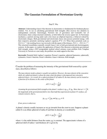
The mass density inside a planet is usually not uniform. However, the mass density of the concentric shells of a spherical planet is about the same when the planet is decomposed into concentric spherical layers As a result, for a spherical planet �� of radius ��, the mass density can be treated as a function of its distance to the center of the planet
��(��)=��0 (1 �� 2��)
Assuming the gravitational field strength at the planet’s surface is ����=�� ≝��0. Show that at �� = 1 2 ��, the magnitude of the gravitational field is less than half that experienced at planet X's surface, yet remains nonzero, that is,
If not, prove it otherwise.
A planet’s density usually increases as we go inwards from the crust to core. Suppose a planet called �� is an oblate spheroid of radius �� and that its density �� is modeled by
��(��)=��0 (1 �� 2��)
where �� is the radial distance from the center, ��0 is constant. The approximate volume of a spherical shell of radius �� and thickness ���� is given by
so the mass in this shell is given by ���� =��(��)��(������������)
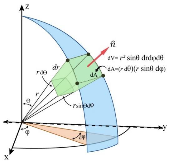
where ��(��) is the mass density as a function of the given coordinates ��∈ℝ3, which yields a more general equation in spherical coordinates
or in Cartesian coordinates,
Therefore, the total mass as a function of �� is given by the integral
Remark 1. The ratio of ���� and ��½�� is
which shows that ���� >��½�� and that ���� ≈6��
THEOREM 1 THE DIVERGENCE THEOREM
Let �� be a compact domain (an enclosed volume) in ℝ3 with piecewise-smooth boundary ����. If �� is a smooth vector field ��=⟨��1(��,��,��),��2(��,��,��),��3(��,��,��)⟩ in ��; then the flux of �� across the boundary ���� of �� is
where �� ̂ is the outward unit normal of ����.
Idea. What we want to show is that the total flux of the vector field across the boundary of our solid matches the triple integral of its divergence inside the solid:
Both sides of the equation break naturally into three pieces, one for each component of the vector field. On the left-hand side, the flux integral splits into contributions from ��1, ��2, and ��3. On the right-hand side, the divergence also splits into three parts, involving the derivatives of ��1, ��2, and ��3 Instead of trying to prove the whole statement all at once, we only show that the two sides match component by component. To keep things concrete, let’s focus on the ��3 part. In other words, we’ll prove that the flux contribution involving ��3 equals the triple integral of ����3/����, i.e. that
Once that’s established, the arguments for ��1 and ��2 follow in exactly the same way (mutatis mutandis)
Proof. Consider the case of special geometry �� that consists of a finite number of smooth pieces that meet along sharp curves. We will first assume that the solid has the special form
where ������ is some subset of the ����-plane. We can further assume that, for each (��,��)∈������, we have ��(��,��)≤��(��,��). Once we handle this simpler case, we’ll extend the argument to any general solid. Let’s start by examining ∯ ��3�� ̂ ⋅��̂���� ���� first. As in the figure below,
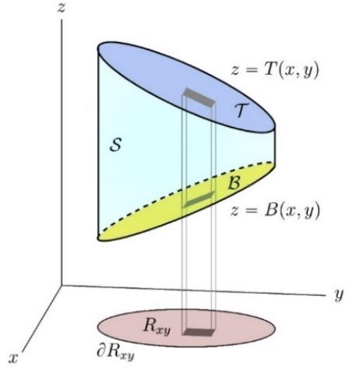
Fig 1 The geometric decomposition perspective in ��3
the boundary surface ���� of this solid has three parts: the top, the bottom, and the sides. Let’s go through them one by one:
• The top �� ={(��,��,��)|�� =��(��,��),(��,��)∈������}:
On ��, we have
The outward normal �� ̂ points upward on ��, which is why we get a “+” sign. So �� ̂ �� ̂���� =�������� and
The flux contribution from the top surface is simply the value of ��3 (the vertical component of the vector field) evaluated at the top, integrated over the whole base region ������
• The bottom ℬ ={(��,��,��)|�� =��(��,��),(��,��)∈������}:
On ℬ, we have
The outward normal �� ̂ points downward on ℬ, which is why we get a “ ” sign So �� ̂ ⋅ �� ̂���� = �������� and
The flux from the bottom surface is therefore minus the integral of ��3 evaluated at the bottom, again over the same base region ������.
• The side is �� ={(��,��,��)|(��,��)∈��������,��(��,��)≤�� ≤��(��,��)}. It turns vertically. Hence on �� the normal vector to ���� is parallel to the xy-plane so that �� ̂ ⋅�� ̂ =0 and
Therefore, all together
By the fundamental theorem of calculus, we have
That’s exactly what we had to show, which is
Now, in the case of general geometry, we drop the assumption on �� that we imposed in the aforementioned case. The key idea behind the proof is that any region �� can be subdivided into “pieces,” each of which satisfies the special assumption we have already considered. For example, take the sausage-shaped solid shown in the figure on the left.
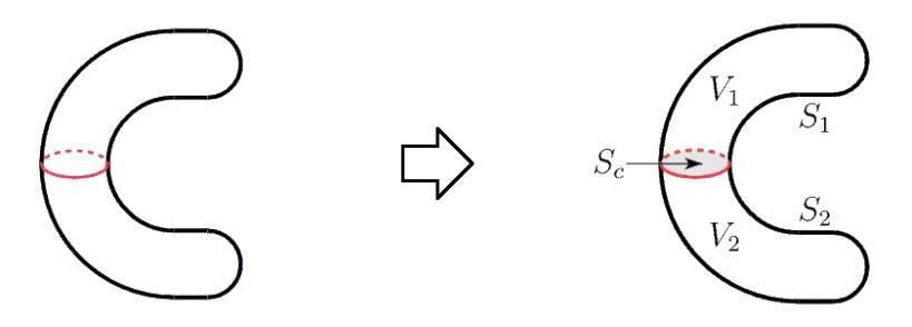
Fig 2. Dividing the geometry into two simpler sub-bodies
Call this solid ��. If we slice it horizontally through its center, we split �� into two halves, ��1 and ��2, as shown in the figure above. This cut also divides the boundary ���� of �� into two parts, ��1 and ��2, as illustrated in the figure on the right above. Note that:
• The boundary ����1 of ��1 is the union of ��1 and the shaded disk ���� (the cut introduced by the cleaver). On ����, the outward normal to ��1 points in the �� ̂ direction.
• The boundary, ����2 of ��2 is the union of ��2 and the shaded disk ���� On ����, the outward normal to ��2 points in the +�� ̂ direction.
Now that the sausage has been split, both ��1 and ��2 satisfy the assumption of the “Special Geometry” case discussed above. So
When we apply the divergence theorem separately to ��1 and ��2, the fluxes across ���� cancel each other out, since the normals point in opposite directions. What remains is exactly the flux through ��1 ∪S2, which is the flux across ����. This shows how the theorem extends naturally from the special geometry to the more general case. Here ���� ↓ is the surface ���� with normal vector �� ̂ and ���� ↑ is the surface ���� with normal vector +�� ̂ The second and fourth integrals are identical except that �� ̂ = �� ̂ in the second integral and �� ̂ =+�� ̂ in the fourth integral. So, they cancel exactly and
as desired. This completes the proof ∎
There are three primary approaches to proving the divergence theorem: the infinitesimal cube method, the parametrization method, and the geometric decomposition method. The first approach partitions the volume into infinitely many microscopic cubes and relies on the cancellation of internal fluxes in the limit. The second method employs local coordinates on the boundary surface, transforming the flux integral through the use of the Jacobian. The third approach the one adopted in this proof decomposes the boundary into a finite number of smooth surface segments and directly sums their flux contributions without explicit parametrization. This method not only avoids the use of Taylor expansions in the first approach to control approximation errors and the need to carefully manage limiting processes, but also avoids the computational complexity associated with the Jacobian matrix used in the second approach
However, most textbooks begin with the first approach: proving the theorem for the case of a rectangular box, and then extending it to a general region. It is worth noting that proving the case of a cube (or rectangular box) is not nearly as difficult as it might sound The idea is simply to divide �� into smaller cuboids whose sides are parallel to the coordinate axes, and then complete the proof in three steps:
(1) Start with the divergence integral and split it by Fubini’s theorem (will be proved later)
(2) Apply the one-dimensional FTC (Fundamental Theorem of Calculus) in the ��-variable.
(3) Recognize the result as the flux of �� through the two ��-faces of the box.
Repeating the same process for the ��- and ��-components, and then adding them together, yields the divergence theorem for a rectangular box.
Proof. Assuming the center of one of the cuboids is defined at ��(��,��,��) with side lengths ����, ����, and ���� Let ��=⟨��1(��,��,��),��2(��,��,��),��3(��,��,��)⟩∈��1(��), that is,
3. By Fubini’s theorem and one-dimensional FTC,
This represents precisely the net flux through the two faces perpendicular to the ��-axis. The same argument applied to the other components yields
Adding the three equalities we get
This proves the divergence theorem for the rectangular box ∎ Now, if we want to prove the theorem for a general region (say, a sphere), we apply the same idea as before: approximate the region by summing up many small cuboids that fit inside the sphere, as illustrated below.
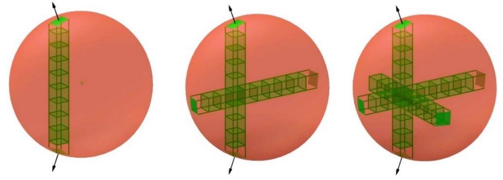
Now let �� ⊂ℝ3 be a region with a piecewise smooth boundary, and let ��:ℝ3 →ℝ3 be continuously differentiable. We already know the Divergence Theorem holds for rectangular boxes. We want to extend it to �� by partitioning the region. We divide ��into��smallnonoverlappingrectangularboxes��1,��2,…,���� suchthat
For
since it is a box, the divergence theorem holds:
where �� ̂ �� is the outward normal to ����. By summing over all boxes, we have
(��⋅�� ̂ ��)����
(��⋅��)����
For the right-hand side, in the limit as the partition becomes finer (i.e., ������ �� ��������(����)→0), we have
For the left-hand side, each internal face appears twice once for each adjacent box with opposite orientations. Hence, their contributions cancel, leaving only the faces on ����:
Finally, as the boxes become arbitrarily small, the sums converge to the integrals over the entire region and its boundary:
With this, we conclude the divergence theorem
So, the theorem is proved for the sphere ∎
Remark 2. We have a partition of our region �� into boxes ��1,��2,…,����.Eachboxhasa diameter,definedas ��������(����)=sup{‖�� ��‖:��,�� ∈����},
i.e., the largest distance between any two points inside ����. The notation “������ �� ��������(����)→0” means “the mesh of the partition goes to zero,” which indicates that we are making the partition finer and finer so that the largest box in the partition shrinks to zero size. This guarantees that our sum over the boxes converges to the integral over the region ��, because the boxes are becoming infinitesimally small.
Remark 3. Using Theorem 1, we can measure the flux of a vector field across the boundary of a domain based on the integral of the divergence of the field over the domain itself.
THEOREM 2 THE GAUSS FLUX THEOREM FOR GRAVITY
Let ��(��) be a neighborhood of ��=(��,��,��) contained in V, that is, a spherical ball �� ≝ {��∈ℝ3 ∶‖��‖≤��} of radius ��, and �� ̂ the outward unit normal on ���� Let �� be a continuously differentiable vector field defined on an open set containing ��; then the flux of �� across the boundary ���� of �� is
Proof. Since �� is calculated from the integral of the point-mass contributions of the masses distributed in ℝ3 , proving this equality requires only showing the same for a mass concentrated at one point, origin for example. By Newton’s law, the gravitational force between two masses ��1 and ��2 at distance �� is equal to ��1��2�� �� 2 . The gravitational field strength is generated by a mass �� located at the origin, according to Newton’s law:
In this field, ��⋅��=0. Consider a small sphere ��0 of radius �� centered at the origin, and let �� be the solid lying between ��0 and ��. By the Gauss-Ostrogradski formula,
As a result, it is sufficient to prove Gauss’s law for sphere ��0. On this sphere the flow ��⋅�� ̂ has the form ��⋅�� ̂ =��(��)�� ̂ ⋅�� ̂ =��(��), which is constantly equal to ���� ��2 according to Newton's law of universal gravitation. Integrating it over the sphere gives
= 4������,
�� being the total mass ∭ ��(��)��3�� �� inside �� with ����, proving the theorem ∎
Remark 4. The vector �� ̂ is the outward unit normal on the boundary of ��, that is, �� ̂ =
Definition 1. A vector that is perpendicular to the plane or a vector and has a magnitude 1 is referred to as a unit normal vector, that is,
Definition 2. Given two nonzero vectors �� and �� in ℝ��, the dot product is defined as,
THEOREM 3 THE DOT PRODUCT THEOREM
Given �� is the angle defined as the unique �� ∈[0,��] between two nonzero vectors �� and ��, the following definition for the dot product between �� and �� is equivalent to Definition 2:
Proof. The Law of Cosines and the magnitudes property of the dot product, ��⋅��=‖��‖2 , allow us to relate

Fig 4. Vector method of deriving the cosine rule.
Using the properties of the dot product, we can rewrite the left side as
Substituting back into the Law of Cosines yields
Definition 3. If �� is a smooth vector field defined on a piecewise smooth oriented surface �� with unit normal vector �� ̂, then the flux of �� across �� is
Remark 5. We know ��⋅����=��⋅��̂���� is true by Definition 3, �� is the radius of spherical Gaussian surface ���� (the boundary of the spherical ball), and �� is the radius of planet ��. In accordance with Definition 1 and Theorem 2, Gauss’s formula yields the equality
where ‖��̂‖=1 and ������(��)= 1. Therefore,
Using the aforementioned theorems, definitions and remarks, we can rewrite the formula as ��(4����2)= 4������
��2 , �������� being the total mass inside the spherical ball of radius �� with boundary ���� of ��. Mass outside the spherical ball makes no contribution. For the case of uniform density, this is equal to �� = 4 3 ����3�� and �� = 4 3�������� Furthermore, we know from Theorem 2,
Due to its conservative nature, the gravitational field must have an associated potential function. In this case, ��= ���� Together with �������� =∭ ��(��)��3�� �� we can rewrite the above equation as
Transforming the left hand integral by Theorem 1 gives
This is true for all volumes ��. By reversing the volume integrals, we obtain ��⋅( ����)=
It follows that the Newtonian gravitational potential ��(��), which is spherically symmetric about a given point in space ��∈ℝ3 , satisfies the gravitational Poisson equation
where �� =‖��‖ is simply the distance of the position from the origin. This is an inhomogeneous linear partial differential equation of elliptic type with a source term that is a function of ��, i.e., ��(��)=4������ For the corresponding total mass contained within the closure ��∪���� (the closed volume bounded by ����), we have
which can be derived from Theorem 1
WHEN
GRAVITATION MEETS QUANTUM MECHANICS: THE ROLE OF SPHERICAL HARMONICS
It is worth noting that the solution approach depends on the choice of coordinate system, with each method carrying its own advantages and limitations. In Cartesian coordinates, the gravitational Poisson equation in ℝ3 is expressed as
for which the equation admits separation of variables Assuming the solution to the Poisson equation has the form
The main goal is to substitute this series expansion for ��(��,��,��) into the Poisson equation and solve 4���� ��(��,��,��)=������ +������ +������. In spherical polar coordinates (radial distance ��, polar angle ��, and azimuthal angle ��), the equation in ℝ3 is then described by
for which the solution of the equation can be represented by spherical harmonics expansion
where ���� ��(��) are the associated Legendre functions of order �� and degree �� which satisfy
the associated Legendre equation when �� and �� are integers, �� ≥0, �� ≤�� ≤�� These functions are of great importance in quantum mechanics as they are used to construct the spherical harmonics a set of special functions reappeared as solutions to the Schrödinger equation for the hydrogen atom in spherical polar coordinates. Poisson’s equation can also be solved in other coordinate systems, but that is beyond the scope of this discussion.
Remark 6. As a matter of convention, the scalar potential of a vector field �� is a function that satisfies ��=����. However, when the vector field �� represents a force so that the force pushes an object from a higher potential to a lower potential, then �� is a function that satisfies ��= ����.
Remark 7. The Poisson equation ��2�� =4������ can be used to measure the gravitational potential when �� is known. When �� =0, the equation becomes homogenous without the source term, which reduces to the Laplace equation.
In a spherical coordinate system, the fundamental solution to ��2�� =4������ can be obtained using the Green function, treating it as a propagator to solve for ��(��), where �� denotes the general coordinate of ��. To proceed, we first review Green’s identities, which are particularly useful for converting integrals involving gradients and divergences into integrals expressed in terms of normal derivatives. With this framework, we then derive the gravitational potential through the Green function and explore cases in which this method may be applied to the measurement of gravitational potential.
THE DERIVATION OF GREEN’S FIRST AND SECOND IDENTITIES
Let us recall Theorem 1, which is the divergence theorem:
We set ��=���� with �� a ��2 scalar function on some region �� ⊂ℝ��, that is, a twice continuously differentiable function on ��, we then obtain
Similarly, but set ��=������ with �� and �� a ��1 scalar function and a ��2 scalar function respectively on some region �� ⊂ℝ��, we then have
Using an extension of the product rule, that is, �� (����)=(����) ��+���� ��, we find the equation to be equivalent to
��(����
��̂)����, �� or alternatively to be equivalent to
This is known as Green’s first identity. By reversing the roles of �� and �� yields
Furthermore, subtracting the above equation from the previous equation we then obtain Green’s second identity, which is valid for any pair of function (��,��) expressed as follows:
Definition 4. A boundary condition is considered symmetric for the Laplace operator ��2 on �� if
for all pairs of functions (��,��) that satisfy the boundary condition.
Remark 8. In Green’s second identity, the term ����, which is equivalent to ���� ���� ̂, denotes the directional derivative of �� in the direction of the outward pointing surface normal �� ̂ of the surface element ����, that is,
Remark 9. Dirichlet, Neumann, and Robin boundary conditions are symmetric.
THE DERIVATION OF GREEN’S REPRESENTATION FORMULA
Now, continue from Green’s second identity, we let �� =��, where �� is the Green function taken to be a fundamental solution of the Laplacian
��2��(��;����)=��(�� ����).
In ℝ3 , without boundary conditions, ��(��,����) has the form
��)=
We shall give a complete proof to this by introducing Fourier transform method later. However, Green’s third identity states that any twice continuously differentiable function (harmonic) �� on ��, i.e., a solution to the homogeneous Poisson equation ��2�� =0, can be expressed as an integral over the boundary ���� as
in which ���� ∈�� and �� is on ���� This is also known as Green’s representation formula, a direct application of Green’s second identity to the pair of functions being the radial solution ��(��) and
used to construct solutions to the Poisson equation for Dirichlet boundary condition.
To prove the Green function possesses the above form, consider the system in the open bounded region �� with boundary ����: ��2��(��)=4������(��) in which �� is a given coordinate vector in ℝ3 such that ��=⟨������������������,������������������,����������⟩, 4������(��) is the source term of the system, and ��(��) is our solution Since ��2 is a linear differential operator, i.e., ��2:����(Ω)→���� 2(Ω) for any open set Ω⊆ℝ�� , the solution to a general system of this type can be expressed as an integral over a distribution of source given by 4������(��): ��(��)=∭��(��;����) �� [4������(����)]��3����
in which the Green function describes the response of the system at the point �� to a point source located at ����: ��2��(��;����)=��(�� ����), and the point source is given by the Dirac delta function ��(�� ����)
THE CONSTRUCTION OF GREEN’S FUNCTION
Rewrite the above equation by setting the source at the origin such that ���� =0, we have
��2��(��)=��(��).
As a matter of convenience, let us introduce a new variable ��=�� ���� in which ���� =0: ���� 2��(��)=��(��).
Now, compute for ��(��) with the aid of Fourier transforms:
3
where �� is a wave vector ��=⟨����,��
and ��=⟨��,��,��⟩ so that
These are the Fourier representation of ��(��) and ��(��) respectively. For the Laplacian of the scalar field �������� we have ��
+����
so that
In the Cartesian coordinate system, let
which is equivalent to that of the one in the general coordinate system
Therefore, we have
Since
Thus,
Now apply the Laplacian operator on the Green function:
By definition, the Laplacian of the Green function is the ��-function:
Matching the integrands on both sides, we have
in which �� is arbitrary. For the integral above, we know the elementary volume under the spherical coordinate system is
The transformation of
demonstrated as follows:
Thus, the function can be integrated over every point in ℝ3 by:
Substituting
Plugging
This is the Dirichlet’s discontinuous integral, which can be tackled by the Laplace transform method or the calculus of residues. We prioritize the Laplace transform technique for now.
First notice that when �� >0, ∫ sin(����) �� ∞ 0 ���� =∫ sin(����) ���� ∞ 0 ��(����).
Due to convenience, let ���� =��, and the form ∫ sin�� �� ∞ 0 ���� follows.
Definition 5. Given a function ��(��) defined for all �� ≥0, the Laplace transform of �� is the function �� defined as follows:
for all values of �� for which the improper integral converges.
By Definition 5, we are aware that ��(��)=ℒ{1}=∫ �� ���� ���� ∞ 0 =�� 1 Notice that the integral ∫ sin�� �� ∞ 0 ���� is equal to the integral ∫ �� 1 ∞ 0 sin������, and therefore we have
THEOREM 4 FUBINI’S THEOREM
Let ��, �� be complete measure spaces, �� be ��×�� measurable. If ∫ |��(��,��)|��(��,��)<∞��×�� then
Proof. In the language of vector calculus, the theorem says that if �� is bounded on the rectangle ℾ≝{(x,y)∶a≤x≤b,c≤y≤d}, then
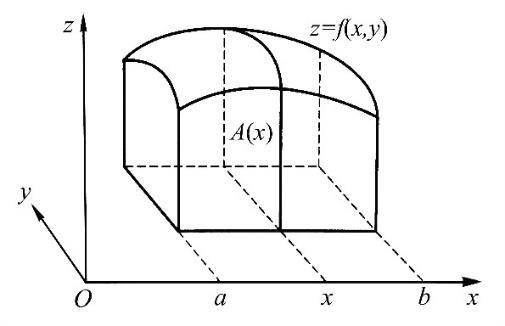
Fig 6 The Illustration of Fubini’s Theorem
The above statement describes a function of two variables ��(��,��) being integrable over a closed rectangle ℾ If there exists an integral ℎ(��)=∫ ��(��,��)������ �� for every �� ∈[��,��], then the integral is integrable on the interval [��,��], which yields
We place the partition points in the interval [��,��]:
�� =��, and write ������ as ���� ���� 1 (�� =1,2, ,��) Clearly, to arrive at the conclusion of the theorem we only need to prove that
Here, ���� represents a random point within the interval [����,���� 1], with �� denoting the maximum value among all ������ Subsequently, position the partition points within the interval [��,��]:
and write ������ as ���� ���� 1 (�� =1,2, ,��). Consider each partition point through [��,��] and [��,��] as lines parallel to the coordinate axes, which divide ℾ into multiple small rectangles (this is a partition of ℾ), and mark ℾ���� as [����,��
1]×[����,���� 1] where �� =1,2,…,��;�� =1,2,…,��. Now, writing
Since ���� ∈[���� 1,����], it yields
Multiplying these inequalities by ������ respectively and adding them up one by one yields
Note that the left and right sides of this inequality are the upper and lower Darboux sums of ��(��,��) upon the partitions made. Since ��(��,��) is integrable on ℾ, when all ������,������ tend to zero, both sides of this inequality tend to
By squeeze theorem for limits, we have
It can be deduced similarly that if ��(��,��) is integrable on ℾ=[��,��]×[��,��], and for all �� ∈ [��,��] the integral ∫ ��(��,��)������ �� exists, then the iterated integral ∫ ����∫ ��(��,��)������ �� �� �� also exists and the following equation holds:
It is important to note, however, that if the target function is positive, the matter of convergence can be bypassed, in which case we have Tonelli’s theorem In physics, Fubini’s theorem means that an n-dimensional object can be represented as a spectrum of layers of shapes made up of (�� 1) dimensions. Thus, a 3D volume can be represented by a set of layers made up of 2D planes
Corollary 2. If we are integrating over the rectangle ℾ=[��,��]�� ×[��,��]�� where ��(��,��) can be factored as ��(��)ℎ(��), then Fubini’s theorem will lead to:
Proof. By Theorem 4, let a function of single variable ��(��) be integrable on the closed interval [��,��], and ℎ(��) be integrable on the closed interval [��,��]. Then, the following holds:
[��,��]×[��,��]
In our problem, according to Theorem 4 we can find a function �� such that ��(��,��)=���� ���� so that |�� ���� sin��|≤��(��,��) for every nonnegative �� and ��. Furthermore, ∫ ��(��,��)∞ 0 ���� =1 for every �� >0; hence, Fubini’s theorem applies:
Since
Accordingly,
When �� =0, we have
we then obtain
When �� <0, we have
However, we choose the value �� 2 since our �� is greater than zero. As a matter of course, we can also obtain the same result by Cauchy’s residue theorem.
Definition 6. Suppose ��(��) is continuous on ℝ except at ��0 ∈(��,��), then the Cauchy principal value is defined by
provided the limit converges.
Remark 10. In Definition 6, ‖�� ��0‖=�� →0 and ‖��‖=�� →∞.
Certainly, ∫ �� 1sin�� ∞ 0 ���� converges and
By definition 6, as we let �� go to infinity and �� go to zero, the integral over the resulting closed contour tends to the Cauchy principal value:
in which �� denotes the principal value of an analytic multivalued function. Therefore, we consider the function ℎ(��)=�� 1������and define the positive indented semicircle, that is, letting �� and �� be �� >�� >0, and consider the region �� bounded by ���� =[ ��, ��]∪���� ∪[��,��]∪���� where ���� is the upper semicircle of ‖��‖=��, and ���� is the upper semicircle of ‖��‖=��.
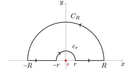
Fig 7 The indented semicircle of Dirichlet’s integral
LEMMA 1 JORDAN’S LEMMA OF ‖�� ��0‖→0
Suppose an arc of the semicircle of radius r centered at ��0 is ���� ≝‖�� ��0‖=��, ������(��)∈ [��,��] and ��(��) is continuous on ���� in which �� is sufficiently small. If
is uniformly valid for �� ∈����, that is, regardless of ������(��)∈[��,��], then
Corollary 3. If ��(��) has a simple pole at ��0 then the following definition for the residue of ��(��) at ��0 is equivalent to the �� of Lemma 1:
Remark 11. Alternatively, Lemma 1 can also be stated as follows:
Suppose ��(��) is holomorphic near �� =��0. Fix ��0 ∈(0,2��). If ���� denotes a counter-clockwise oriented arc of angle ��0 on the circle of radius �� centered at ��0, then
Proof. By the substitution �� =��0 +�������� with the fact that ���� =������������ where ���� =arg(����), then
which clearly goes to zero when ‖�� ��0‖=�� →0. This completes the proof ∎
Remark 12. If �� =�������� with �� >0 and �� ∈( ��,��], then
in which the ������ is an angle, while the ������ is its measure. This implies that principal argument always lies between �� to ��. In addition, multi-valued nature of ������(��) can be visualized by using Riemann surfaces.[1]
LEMMA 2 JORDAN’S LEMMA OF ‖��‖→∞
Suppose ��(��) is continuous on the semicircle of radius �� in the upper half plane ���� ≝‖��‖=�� in which �� =��������,�� ∈[0,��] for �� to be sufficiently large and
‖��‖=��→+∞
is uniformly valid on ����, that is, regardless of ������(��)∈[0,��], then
where �� >0.
Proof. Since ������ ��→+∞��(��)=0 is valid uniformly, ∀�� >0 there exists ���� >0 so that when �� >���� there is an inequality for every �� ∈ℂ such that |��(��)|=������ 1, and therefore
By Jordan’s inequality
proving the lemma ∎
Since ℎ(��) is continuous on ���� and analytic within �� enclosed by ����, by Cauchy’s integral theorem:
Therefore, it implies
By Lemma
By Lemma
Consequently,
so that, by taking imagery parts, we obtain
However, we can also evaluate it directly by using properties of definite integrals,
and let �� = �� and
=
, by changing the signs of the limits of integration we obtain
Consequently,
Plugging the value into the Green function yields
By reversing the roles of �� and �� ����, we obtain the Green function
THE SEEKING OF THE FUNDAMENTAL SOLUTION OF THE POTENTIAL FIELD
Substituting the result into the equation of the potential field ��(��) yields the general solution to Poisson’s equation in which ������ ��→∞ ��(��)=0:
The expression represents the sum of all mass components contributing to the total potential on a given coordinate. The integral of a spherical symmetric mass over an external point can be calculated analytically for certain cases, resulting in a function of the distance to the center of the sphere described as follows:
Recall the gravitational field strength is the magnitude of the gravitational field. This shows that
which matches the outcome done by Gauss’s law
Now back to the original problem, the function of density ��(��) is well-defined so the gravitational field strength can be calculated as follows: (suppose �� is the radial displacement of the Gaussian sphere, that is, the distance of the observation point)
For ��>��: (The field strength on the surface of planet ��: inversely proportional to ��)
Since the observation point is located outside planet ��, we have
��=��:
For ��<��: (The field strength inside planet ��: proportional to ��)
Since the observation point is located inside planet �� and its coordinate is �� =�� ��, then all spherical shells that have radius exceeding �� do not contribute to the gravitational field at the observation point. Correspondingly, we obtain
If we let �� =�� �� in which �� is the distance from the surface of the planet to the radius of the Gaussian surface, we have
For ��=½��: (The field strength on the surface of the inner solid sphere (covered by the Gaussian surface) of radius ½�� enclosed by planet ��: inversely proportional to ��)
Since the observation point is located inside planet �� but outside the inner solid sphere and its coordinate is ��, then all spherical shells that have radius exceeding �� do not contribute to the gravitational field at the observation point. Correspondingly, we have
Given the fact that we have
by comparing
and ��½�� we obtain
This shows that the gravitational field strength at ��=½�� is greater than ½���� but not equal to ���� ∎
ERROR ANALYSIS OF THE OFFICIAL SOLUTION BY TSINGHUA UNIVERSITY
The official solution for this problem concludes that at �� =½��, the gravitational field strength �� is smaller than ½��0. This conclusion is based on an incorrect estimate of the mass enclosed within the Gaussian surface at �� =½��.
The solution states
However, a direct calculation using the given density function ��(��)=��0 (1 �� 2��) shows the exact enclosed mass is
Comparing this to the bounds given
The actual mass, 0.1625����, is greater than ⅛����, not smaller. This shows that the initial estimate is incorrect, which leads to a wrong conclusion about the gravitational field strength. The field is calculated as
Therefore, at �� =½��:
The surface field becomes
If ��½�� <⅛���� were true, then ��
, and the ratio is
0. But since ��
=0.1625����, we get
This completes the calculation and is clearly greater than ��.������
The official solution’s error stems from a faulty mass estimation. The correct calculation proves that ��½�� >½��0, making option E the true statement.