Chapter 1 Solutions
1.1
a) Driving a car
Please see either jogging, cycling, stirred tank heater, or household thermostat for a representative answer.
b) Two sample favorite activities: Jogging
i. Objectives:
Jog intensely (heart rate at 180bpm) for 30 min. Smooth changes in jogging intensity and speed.
ii. Input Variables:
Jogging Rate – Manipulated input
Shocking surprises (dogs, cars, etc.)–Disturbance
iii. Output Variable
Blood Oxygen level –unmeasured
Heartbeat – measured. Breathing rate – unmeasured
iv. Constraints:
Hard: Max Heart Rate (to avoid heart attack! death)
Hard: Blood oxygen minimum and maximum
Soft: Time spent jogging
v. Operating characteristics: Continuous during period, Semi Batch when viewed over larger time periods.
vi. Safety, environmental, economic factors: Potential for injury, overexertion
vii. Control: Feedback/Feedforward system. Oxygen level, heartbeat, fatigue all part of determining action after the fact. Path, weather is part of feedforward system.
Cycling
i. Objectives: Ensure stability (don't crash)
Enjoy ride. Prevent mechanical failure.
ii. Input Variables – Manipulated
Body Position
Steering
Braking Force
Gear Selection
Input Variables – Disturbance
Weather Path Conditions
Other people, animals
iii. Output Variables – Measured: Speed
Direction
Caloric Output (Via electron monitor)
Output Variables – Unmeasured: Level of enjoyment
Mechanical integrity of person and bicycle
Aesthetics (smoothness of ride)
iv. Constraints – Hard:
Turning radius
Mechanical limits of bike and person
Maximum fatigue limit of person
Constraints – Soft:
Steering dynamics that lead to instability before mechanical failure (i.e. you crash, the bike doesn't break)
Terrain and weather can limit enjoyment level.
v. Operation: Continuous: Steering, weight distribution, terrain selection within a path, pedal force Semi batch: Gear selection, braking force Batch: Tire pressure, bike selection, path selection
vi. Safety, environment, economics: Safety: Stability and mechanical limits prevent injury to rider and others Environment: Trail erosion, noise Economics: Health costs, maintenance costs.
vii. Control Structure: Feedback: Levels of exertion, bike performance is monitored and
ride is adjusted after the fact
Feedforward Path is seen ahead and ride is adjusted accordingly.
c) A stirred tank heater
i. Objectives
Maintain Operating Temperature
Maintain °ow rate at desired level.
ii. Input Variables:
Manipulated: Added heat to system
Disturbance: Upstream Flow rate and conditions
iii. Output Variables – Measured: Tank fluid temperature, Outflow.
iv. Constraints:
Hard: Max inflow and outflow as per pipe size and valve limitations
Soft: Fluid temperature for operating objective
v. Operating conditions: Continuous fluid flow adjustment, continuous heating adjustment
vi. Safety, Environmental, Economic considerations: Safety: Tank overflow, failure could cause injury Economics: Heating costs, spill costs, process quality costs Environmental: Energy consumption, contamination due to spills of hot water.
vii. Control System: Feedback:
Temperature is monitored, heating rate is adjusted Feedforward: Upstream flow velocity is used to predict future tank state and input is adjusted accordingly.
d) Beer Fermentation
Please see either jogging, cycling, stirred tank heater, or household thermostat for a representative answer.
e) An activated sludge process.
Please see either jogging, cycling, stirred tank heater, or household thermostat for a representative answer.
f) A household thermostat
i. Objectives:
Maintain comfortable temperature.
Minimize energy consumption.
ii. Input Variables:
Manipulated: Temperature setting
Disturbance: Outside temperature, energy transmission between house and environment
iii. Output Variables:
Measured: Thermostat reading
Unmeasured: Comfort level
iv. Constraints:
Hard: Max heating or cooling duty of system
Soft: Max or minimum temperature for comfort
v. Operating conditions: Continuous heating adjustment, continuous temperature reading.
vi. Safety, Environmental, Economic considerations: Safety: heater may be an electrical or burning hazard
Economics: Heating costs
Environmental: Energy consumption.
vii. Control System: Feedback; temperature is monitored, heating rate is adjusted after the fact.
g) Air traffic control
Please see either jogging, cycling, stirred tank heater, or household thermostat for a representative answer.
h) Taking a shower
A common multivariable control problem that we face every day is taking a shower. A simplified process schematic is shown in the Figure below. We analyze this process step by step.
i. Objectives:
To become clean
To be comfortable (correct temperature and water velocity as it contacts the body)
To “look good” (clean hair, etc)
To become refreshed
To simplify our analysis, for the rest of the problem we discuss how we can satisfy the second objective (to maintain water temperature and flow rate at comfortable
1.1h Shower problem.
A common multivariable control problem that we face every day is taking a shower. A simplified process schematic is shown in the Figure below. We analyze this process step by step.
i. Control objectives: Control objectives when taking a shower include the following:
a. to become clean
b. to be comfortable (correct temperature and water velocity as it contacts the body)
c. to “look good” (clean hair, etc.)
d. to become refreshed
To simplify our analysis, for the rest of the problem we discuss how we can satisfy the second objective (to maintain water temperature and flow rate at comfortable values). Similar analysis can be performed for the other objectives.
ii. Input variables: The manipulated input variables are hot-water and cold-water valve positions. Some showers can also vary the velocity by adjustment of the shower head. Another input is body position you can move into and out of the shower stream. Disturbance inputs include a drop in water pressure (say, owing to a toilet flushing) and changes in hot water temperature owing to “using up the hot water from the heater.”
iii. Output variables: The “measured” output variables are the temperature and flow rate (or velocity) of the mixed stream as it contacts your body.
iv. Constraints: There are minimum and maximum valve positions (and therefore flow rates) on both streams. The maximum mixed temperature is equal to the hot water temperature and the minimum mixed temperature is equal to the cold water temperature. The previous constraints were hard constraints they cannot be physically violated. An example of a soft constraint is the mixed-stream water temperature you do not want it to be above a certain value because you may get scalded. This is a soft constraint because it can physically happen, although you do not want it to happen.
v. Operating characteristics: This process is continuous while you are taking a shower but is most likely viewed as a batch process, since it is a small part of your day. It could easily be called a semicontinuous (semibatch) process.
vi. Safety, environmental, and economic considerations: Too high of a temperature can scald you this is certainly a safety consideration. Economically, if your showers are too long, more energy is consumed to heat the water, costing money. Environmentally (and economically), more water consumption means that more water and wastewater must be treated. An economic objective might be to minimize the shower time. However, if the shower time is too short, or not frequent enough, your clothes will become dirty and must be washed more often increasing your clothes-cleaning bill.
vii. Control structure: This is a multivariable control problem because adjusting either valve affects both temperature and flow rate. Control manipulations must be “coordinated,” that is, if the hot-water flow rate is increased to increase the temperature, the cold-water flow rate must be decreased to maintain the
Hot waterCold water
same total flow rate. The measurement signals are continuous, but the manipulated variable changes are likely to be discrete (unless your hands are continuously varying the valve positions).
Feedback control: As the body feels the temperature changing, adjustments to one or both valves is made. As the body senses a flow rate or velocity change, one or both valves are adjusted.
Feed-forward control: If you hear the toilet flush, you move your body out of the stream to avoid the higher temperature that you anticipate. Notice that you are making a manipulated variable change (moving your body) before the effect of an output (temperature or flow rate) change is actually detected.
Some showers may have a relatively large time delay (or dead time) between when a manipulated variable change is made and when the actual output change is measured. This could happen, for example, if there was a large pipe run between the mixing point and the shower head (this would be considered an input time delay). Another type of time delay is measurement dead time, for example if your body takes a while to detect a change in the temperature of the stream contacting your body.
Notice that the control strategy used has more manipulated variables (two valve positions and body movement) than measured outputs (total mixed-stream flow rate and temperature).
In the shower example, the individual taking the shower served as the controller. The measurements and manipulations for this example are somewhat qualitative (you do not know the exact temperature or flow rate, for example). Most of the rest of the textbook consists of quantitative controller design procedures, that is, a mathematical model of the process is used to develop the control algorithm.
1.2l AP problem. Automated insulin delivery (closed-loop artificial pancreas) for individuals with type 1 diabetes. See Figure 1-8 and Module 12.
Literature Review: Bequette BW. Automated Insulin Dosing for Type 1 Diabetes. Chapter in Encyclopedia of Systems and Control. Baillieul J and Samad T (eds). Springer (2020). https://doi.org/10.1007/978-1-4471-5102-9 100131-1
i. This encyclopedia article provides an overview of automated insulin delivery devices. It is interesting because these algorithms and devices represent an excellent opportunity for individuals with type 1 diabetes to no longer need to be constant monitoring their glucose values and making frequent insulin (and/or meal) adjustments, but can let the closed-loop algorithm make these decisions.
While neither the model nor the algorithms are directly presented, a number of plot stress the important steady-state and dynamic problems involved. A number of algorithms are suggested, including PID and MPC.
ii. Words and concepts: PID, MPC, fuzzy logic, fault detection, simulation models.
1.3h CGM. Instrumentation Search. Select one of the following measurement devices and use Internet resources to learn more about it. Determine what types of signals are input to or output from the device.
The following NIDDK source provides a solid background on continuous glucose monitoring: https://www.niddk.nih.gov/health-information/diabetes/overview/managing-diabetes/continuous-glucosemonitoring
The following description is directly from the website:
" How does a continuous glucose monitor work?
A continuous glucose monitor (CGM) estimates what your glucose level is every few minutes and keeps track of it over time.
A CGM has three parts. First, there is a tiny sensor that can be inserted under your skin, often the skin on your belly or arm, with a sticky patch that helps it stay there. These sensors are called disposable sensors. Another type of CGM sensor called an implantable sensor may be placed inside your body. CGM sensors estimate the glucose level in the fluid between your cells, which is very similar to the glucose level in your blood. Sensors must be replaced at specific times, such as every few weeks, depending on the type of sensor you have.
The second part of the CGM is a transmitter. The transmitter sends the information, without using wires, to the third part, a software program that is stored on a smartphone, on an insulin pump, or on a separate device called a receiver."
While not discussed, it should be clear that the sensors are measuring the interstitial fluid glucose, and that there may be a time lag between the capillary blood and interstitial fluid glucose values.
The article goes on to discuss "real time" vs. "intermittent-scan" monitors. The real time monitors are more usually for implementation in a automated insulin delivery device, while the intermittent-scan monitors are useful for someone that simply wants to scan their values an infrequent intervals. In both cases the monitors are indirectly inferring the blood glucose by sending signals that are related to the interstitial fluid glucose values.
1.5 Surge Drum Problem. Consider Example 1.1, the liquid surge vessel, which assumed that the outlet stream flowrate was manipulated. Now, perform a complete analysis assuming that the inlet stream flowrate is manipulated.
a. Draw the instrumentation diagram for this problem.
b. Should the control valve on the inlet stream be fail-open or fail-closed? Why?
c. Draw the feedback block diagram for this problem.
d. Develop the instrumentation diagram for combined feedforward and feedback control for this problem.
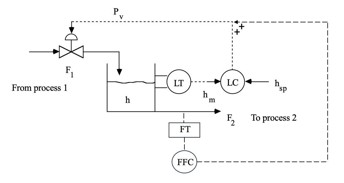
a. The control and instrumentation diagram for a feedback control strategy for scenario 1 is shown below.
Notice that the level transmitter (LT) sends the measured height of liquid in the tank ( hm) to the level controller (LC). The LC compares the measured level with the desired level ( hsp, the height setpoint) and sends a pressure signal (Pv) to the valve. This valve top pressure moves the valve stem up and down,
changing the flow rate through the valve ( F1). If the controller is designed properly, the flow rate changes to bring the tank height close to the desired setpoint. In this process and instrumentation diagram we use dashed lines to indicate signals between different pieces of instrumentation.
b. The control valve should be specified as fail-closed or air-to-open, so that the tank will not overflow on loss of instrument air or other valve failure.
c. A simplified block diagram representing this system is shown in below. Each signal and device (or process) is shown on the block diagram. We use a slightly different form for block diagrams when we use transfer function notation for control system analysis in Chapter 6. Note that each block represents a dynamic element. We expect that the valve and LT dynamics will be much faster than the process dynamics. We also see clearly from the block diagram why this is known as a feedback control “loop.” The controller “decides” on the valve position, which affects the inlet flow rat e (the manipulated input), which affects the level; the outlet flow rate (the disturbance input) also affects the level. The level is measured, and that value is fed back to the controller [which compares the measured level with the desired level (setpoint)].
d. Feedforward and Feedback control is shown below
a. Fluidized Catalytic Cracking Unit
i. Summary of paper:
A fluidized catalytic cracking unit (FCCU) is one of the typical and complex processes in petroleum refining. Its principal components are a reactor and a generator. The reactor executes catalytic cracking to produce lighter petro-oil products. The regenerator recharges the catalyst and feeds it back to the reactor. In this paper, the authors test their control schemes on an FCCU model. The model is a nonlinear multi-input/multi-output (MIMO) which couples time varying and stochastic processes. Considerable computation is needed to use model predictive process control algorithms (MPC). Standard PID control gives inferior performance. A simplified MPC algorithm can reduce the number of parameters and computational load while still performing better than a PID control method.
ii. Familiar Terms: Constraint, nonlinearity, control performance, MPC, unmeasured disturbance rejection, modeling, simulation.
b. Reactive Ion Etching
Please see FCCU for a representative answer.
c. Rotary Lime Kiln
Please see FCCU for a representative answer.
d. Continuous Drug Infusion
Please see FCCU for a representative answer.
e. Anaerobic Digester
Please see FCCU for a representative answer
f. Distillation
Please see FCCU for a representative answer.
g. Polymerization reactor
Please see FCCU for a representative answer
h. pH
Please see FCCU for a representative answer.
i. Beer Production
Please see FCCU for a representative answer.
j. Paper Machine Headbox
Please see FCCU for a representative answer.
k. Batch Chemical Reactor
Please see FCCU for a representative answer.
l. AP problem.
Automated insulin delivery (closed-loop artificial pancreas) for individuals with type 1 diabetes. See Figure 1-8 and Module 12. Literature Review: Bequette BW.
Automated Insulin Dosing for Type 1 Diabetes. Chapter in Encyclopedia of Systems and Control. Baillieul J and Samad T (eds). Springer (2020).
https://doi.org/10.1007/978-1-4471-5102-9 100131-1
i. Summary of Paper
This encyclopedia article provides an overview of automated insulin delivery devices. It is interesting because these algorithms and devices represent an excellent opportunity for individuals with type 1 diabetes to no longer need to be constant monitoring their glucose values and making frequent insulin (and/or meal) adjustments but can let the closed-loop algorithm make these decisions. While neither the model nor the algorithms are directly presented, a number of plots stress the important steady-state and dynamic problems involved. A number of algorithms are suggested, including PID and MPC.
ii. Words and concepts: PID, MPC, fuzzy logic, fault detection, simulation models.
1.3
a. Vortex-shedding flow meters
The principal of vortex shedding can be seen in the curling motion of a flag waving in the breeze, or the eddies created by a fastmoving stream. The flag outlines the shape of air vortices as the flow past the pole. Van Karman produced a formula describing the phenomena in 1911. In the late 1960’s the first vortex shedding meters appeared on the market. Turbulent flow causes vortex formation in a fluid. The frequency of vortex detachment is directly proportional to fluid velocity in moderate to high flow regions.
At low velocity, algorithms exist to account for nonlinearity. Vortex frequency is an input, fluid velocity is an output.
b. Orifice-plate flow meters
Please see vortex–shedding flow meters for a representative answer.
c. Mass flow meters
Please see vortex–shedding flow meters for a representative answer.
d. Thermocouple based temperature measurements.
Please see vortex–shedding flow meters for a representative answer.
e. Differential pressure measurement
Please see vortex–shedding flow meters for a representative answer.
f. Control Valves
Please see vortex–shedding flow meters for a representative answer.
g. pH
Please see vortex–shedding flow meters for a representative answer.
h. Continuous Glucose Monitor (CGM) to measure blood glucose level.
Instrumentation Search. Select one of the following measurement devices and use Internet resources to learn more about it. Determine what types of signals are input to or output from the device.
The following NIDDK source provides a solid background on continuous glucose monitoring: https://www.niddk.nih.gov/healthinformation/diabetes/overview/managingdiabetes/continuous-glucose-monitoring
The following description is directly from the website:
" How does a continuous glucose monitor work?
A continuous glucose monitor (CGM) estimates what your glucose level is every few minutes and keeps track of it over time.
A CGM has three parts. First, there is a tiny sensor that can be inserted under your skin, often the skin on your belly or arm, with a sticky patch that helps it stay there. These sensors are called disposable sensors. Another type of CGM sensor called an implantable sensor may be placed inside your body. CGM sensors
estimate the glucose level in the fluid between your cells, which is very similar to the glucose level in your blood. Sensors must be replaced at specific times, such as every few weeks, depending on the type of sensor you have.
The second part of the CGM is a transmitter. The transmitter sends the information, without using wires, to the third part, a software program that is stored on a smartphone, on an insulin pump, or on a separate device called a receiver."
While not discussed, it should be clear that the sensors are measuring the interstitial fluid glucose, and that there may be a time lag between the capillary blood and interstitial fluid glucose values.
The article goes on to discuss "real time" vs. "intermittent-scan" monitors. The real time monitors are more usually for implementation in a automated insulin delivery device, while the intermittent-scan monitors are useful for someone that simply wants to scan their values an infrequent intervals. In both cases the monitors are indirectly inferring the blood glucose by sending signals that are related to the interstitial fluid glucose values.
1.4
No solutions are required to work through Module 1 1.5 1.6
a. The main objective is to maintain the process fluid outlet temperature at a desired setpoint of 300 C.
b. The measured output is the process fluid outlet temperature.
c. The manipulated input is the fuel gas flowrate, specifically the valve position of the fuel gas control valve.
d. Possible disturbances include process fluid flowrate, process fluid inlet temperature, fuel gas quality, and fuel gas upstream pressure.
e. This is a continuous process.
f. This is a feedback controller.
g. The control valve should be fail-closed. Increasing air pressure to the valve will then increase the valve position and lead to an increase in flowrate. Loss of air to the valve will cause it to close. The gain of the valve is positive because an increase in the signal to the valve results in an increase in flow.
h. It is important from a safety perspective to have a fail-closed valve. If the valve failed to open, there might not be enough combustion air, causing a loss of the flamethis could cause the furnace firebox to fill with fuel gas, which could then re-ignite under certain conditions. Although the combustion air is not shown, it should be supplied with a small stoichiometric excess. If there is too much excess combustion air, energy is wasted in heating up air that is not combusted. If there is too little excess air, combustion will not be complete, causing fuel gas to be wasted and pollution to the atmosphere. The process fluid is flowing to another unit. If the process fluid is not at the desired setpoint temperature, the performance of the unit (reactor, etc) may not be as good as desired, and therefore not as profitable.
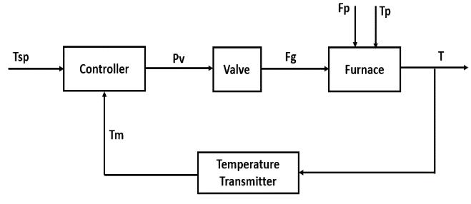
i. The control block diagram for the process furnace is shown below in Figure 1. Where the signals as
Follows:
• Tsp: Temperature setpoint
• pv: Valve top pressure
• Fg: Fuel gas flowrate
• Fp: Process fluid flowrate
• Tp: Process fluid inlet temperature
• T: Temperature of process fluid outlet
• Tm: Measured temperature
The problem statement tells us that the gasoline is worth $500,000 a day. A 2% increase in value is:
We are also given that revamping will cost $2,000,000. We can now calculate the time required to pay back the control system investment.
Therefore, we know it will take 200 days to pay off the investment. 1.8
We know from the problem statement that the inlet ( and outlet ( flowrates can be represented with the following equations: = 50 + 10
The change in volume as a function of time is:
Substituting what we know:
Simplifying
Rearranging the equation
Taking the integral of both sides
Using basic calculus to solve
We know the initial tank volume is 500 liters. The equation tells us how the volume of the tank will vary with time. This can also be seen visually in Figure 2 below.
Figure 1-1: Control block diagram of process furnace
1.10
a.The objective is to maintain a desired blood glucose concentration by insulin injection. Insulin is the manipulated input and blood glucose is the measured output. As performed by injection, the input is really discrete and not continuous. Also, glucose is not continuously measured, so the measured output is discrete. Disturbances include meal consumption and exercise. Feedforward action is used when a diabetic administers an injection to compensate for a
Figure 1-2: Liquid volume as a function of time meal. Feedback action occurs when a diabetic administers more or less insulin based on a blood glucose measurement. It is important not to administer too much insulin, because this could lead to too low of a blood glucose level, resulting in hypoglycemia.
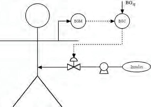
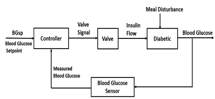
b.A process and instrumentation diagram of an automated closed-loop system is shown in Figure 3 below. For simplicity, this is shown as a pump and valvearrangement. In practice, the pump speed would be varied. The associated control blockdiagramis shown in figure 4 below.

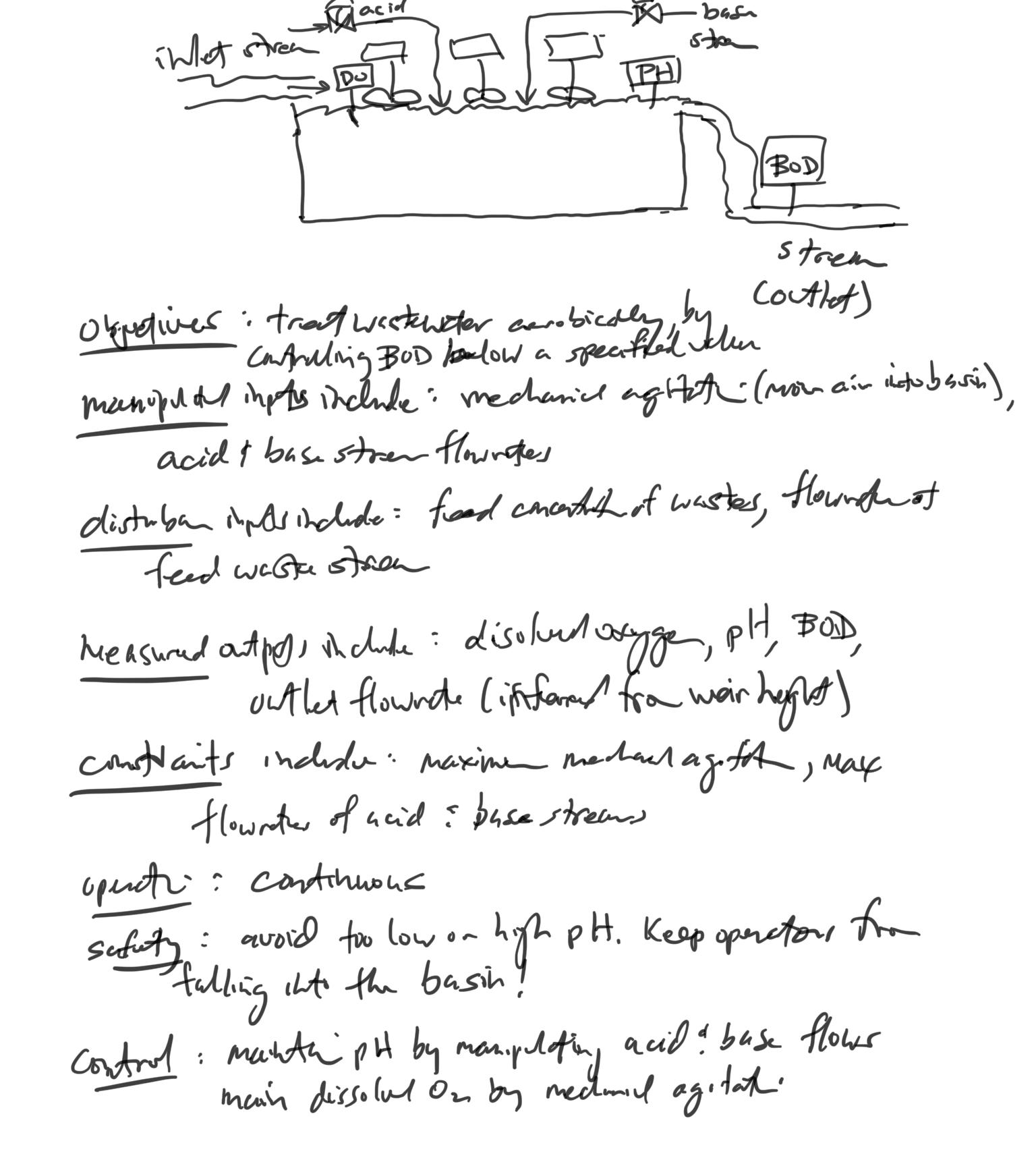
1.13. An aeration basin (a very large “vessel”) is used to continually treat a wastewater stream aerobically. A number of mechanical agitators at the surface can be used to “pump” air into the basin; these can be independently turned on or off to change the level of dissolved oxygen in the basin. The microbes that “eat” the waste function best in a small pH range. Acid and base stream flowrates into the basin can be manipulated. An analytical device that can measure the concentration of waste material in terms of BOD (biochemical oxygen demand) is placed in the outlet stream of the basin. The liquid level in the basin is relatively constant, since the effluent flows over a weir. The outlet flowrate can be estimated by the height of liquid over the weir. Provide a sketch of this process and discuss it in the context of a control problem, identifying objectives, disturbances, etc.

1.14. A gas surge drum, shown below, is used to buffer the effect of gas flow between two operating used. It is important that the gas drum pressure be controlled not to exceed low and high pressure limits. Consider two possible scenarios: (a) the inlet flowrate (qi) is manipulated, and (b) the outlet flowrate (q) is manipulated. In each case, sketch the process and instrumentation diagram with a pressure sensor, controller and control valve. Discuss whether the control valve should be fail-open or fail-closed.
1.15 Consider the temperature control strategy shown below, under two different scenarios: (a) an endothermic reaction, and (b) and exothermic reactor. For each case, discuss whether the jacket fluid is a hot or a cold stream. Also discuss whether the control valve should be designed to fail-open or fail-closed.
a. Endothermic Reaction. The jacket fluid will be a hot stream and the control valve should fail closed to make certain that the reactor does not overheat.
b. Exothermic Reaction. The jacket fluid will be a cold stream and the control valve should fail open to make certain that the reactor does not overheat, possibly causing an explosion.
The modeling equation is
At steady state
Thus,we can conclude that it is a self–regulating system, as for a change in input it will attain a new steady–state.
The sketch of the steady–state input–output curve should look like figure 2-1
The inlet and outlet flow are the same. Thus
For this part we need to integrate
From the initial state of T= The Euler formula is: xk+1 = xk + ∆
Where f ( ) is the right hand side of the differential equation, and x is the state, in this case T. using ∆t = 0.5, and for a total of 2 minutes, we have
2.2
The model equations are:
a. At steady–state, the volume will not change, as
Figure 2-2 shows the curve of the solution found using MATLAB’S ode45, with the circles marking the point of the Euler solution.
Since the model equation have only two states, we have to assume the following are constant:
Density of the liquid (p), temperature (T), the ideal gas constant (R) and the molecular weight of the gas (MW).
Starting with the balance of the liquid mass in the system, we have
Solving at steady-state, we get
We need to meet a yearly production, so our final constraint is
Where S = is our conversion factor, assuming 350 days of operation in a year. then,
For the balance of the mass of gas
From the ideal gas law where the volume of gas is then,
Solving for the flowrate, we get Fs =
Now we need to consider the second reactor in series, which will also change the flowrate needed to meet production levels. The equations for the second reactor are
And using the previously derived expressions for and
Solving at steady-state, we get
Again, we need to meet production levels, so
Thus, our model equations are.
2.4
Since we have a larger volume than the example, we have to calculate the flow rate for a single reactor as well. Our volume is V =106.9444ft3 the equations for the first tank are
Solving the flowrate, we get Fs =
Thus we have a savings of 16.98% using the two reactors in series over a single one.
The resulting graph should be the same as figure 2-5 except that the time range from -1 to 0 will not appear.
2.6
We need equations whose states are V and CA, then
Our two equations are
2.7
a. The modeling equations are
b. At steady-state we can solve the following equations
Rearranging the first equation, we have the quadratic The positive root gives us
Rearranging the second equation, we get the quadratic
The positive root gives us
c. To linearize, we have the functions
And using the state and input variables as defined, we have
d. Evaluating these coefficients at our steady-state, we have
e. Since , it is straightforward to showthat.
f. Using MATLAB, the eigenvalues are -0.320156 and -1.25.
Analytically,we have
Thus,the eigenvalues are
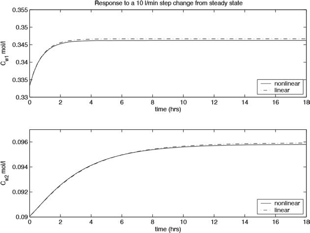
g. Figure 2-3 shows the plot for the linear and nonlinear responses; as it can be seen, the extraction requirements are still met.
h. if the order of the reaction vessels is reversed, the steady-state equations we have to solve are
Solving then we have thus, the extraction requirements are no longer met.
a. solve the following simultaneous equations using the parameters and steady-state values provided:
Then
b. applying the equations for the elements of the linearization matrices
c. heater .m file should be like the example in the book (p.73)
d. using delJ= 0, run code 45to solve the equations defined in heater.m, then plot the two states vs. time.The result should be constant values that match thesteady states for all time.
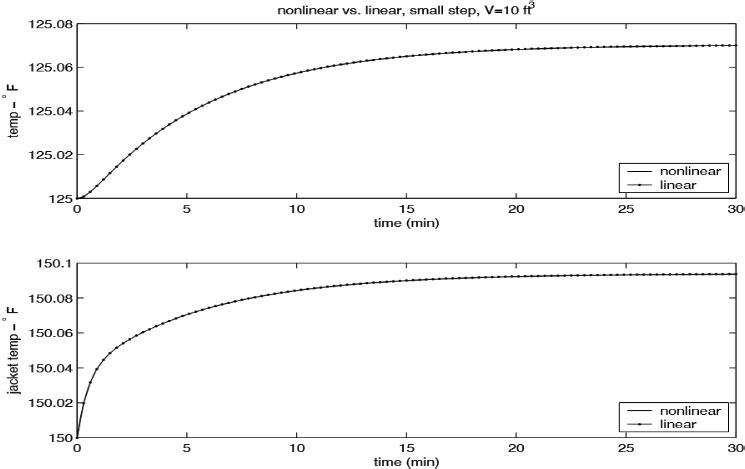
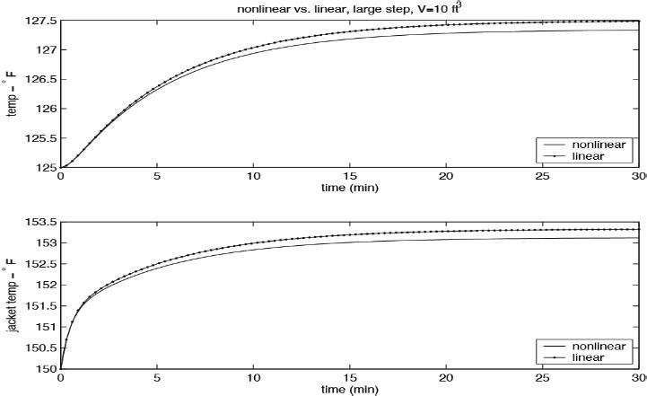
e. To get the desired plots for the two step responses, the m–file shown in pages 74-75 can be used, starting with the definition of the state space linear model. Since the model is linear, the output of the step response command can be scaled accordingly forsteps of different sizes by just multiplying by delFj. Figures 4(a) and 4(b) show the responses for a
Figure 2-3: Plot for 2.7g
small (0.2% change in ) and a large (10% change in ) steps, respectively.
f. Since we know for the small vessel, and we are assuming that U remains constant, we can find the value of for a larger volume as
Modeling the vessel as a cylinder, the volume is , and the area is A = 2.25π . We can then calculate the area of the small vessel as a function of its volume, for which we get
Similarly, we have the area of the larger vessel in terms of its volume.
2-4: Plot for 2.8e (a) small step of 0.2% (b) large step of 10%
and the ratio are is
g. Solve the following two simultaneous equations using the value of calculated for the large vessel
Then We can already see that the steady–state jacket temperature has gone up, so we want to know how large we can make the vessel before the jacket temperature approaches the inlet jacket temperature. We can solve the following equation, using , as we want to maintain the residence time. We also use the expression in terms of the volume that we found in part f
Then .
h. Applying the equations for the elements of the linearization matrices using the steady state for the larger vessel, we have
(b)
Figure
The eigenvalues for the system with the large vessel are at and While for the system with the smaller vessel, they are and . They are very close to each other;thus the speed of the response will be similar for both vessels
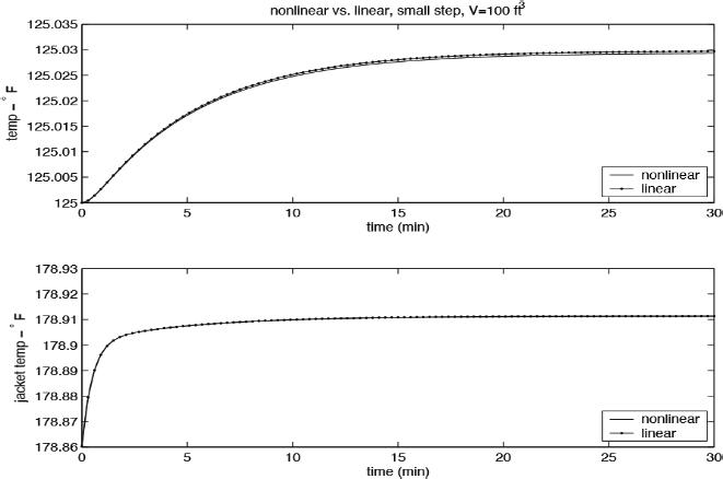
i. Figure 2-5 shows the response to a step of . Comparing this to figure 4(a), we can see that both linear model responses are practically the same as the nonlinear model response. The change in temperatures is also minor, as the change in jacket flow rate is small (0.2% of the steady state value in both cases).
j. Figure 2-6 shows the response to a step of 10% of the steady state jacket flow rate. Comparing this to figure 4(b), we can see that both linear model.
responses are close to the nonlinear model response, butthere is anoffset in the steady state. The change intemperatures is also more marked, and larger in the caseof the smaller reactor, as would be expected due to the smaller volume.
2.10
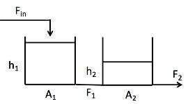
Consider two interacting tanks in series, with a specified inlet volumetric flowrate (Fin) to the first tank, and outlet flowrate from tank 1 into tank 2 proportional to the square root of the tank height differences, and the outlet flowrate from tank 2 proportional to the square root height of liquid in tank 2 (flow coefficients ). Notice that, if the height of tank 2 is initially higher than that in tank 1, the flow could be from tank 2 back to tank 1; that is, F1 could be negative. Assume that the cross-sectional areas (A1 and A2) of the tanks are constant butmay differ for the two tanks.
a. state your assumption about fluid density and write the modeling equation using tank heightas the state variables.
Material balance aroundtank 1
Material balance around tank 2
b. Solve for the steady-state tank heights, as a function of the parameters and inlet flowrate
Steady-state, From (1)
From (2)
Similarly, => => =>
c. Write a MATLAB function file to be used by ode23s; you may wish to use the abs and sign functions. Use the following values , . function xdot = TwoIntTnkNL(t,x,par,u)
% two interacting tank problem with nonlinear height-flow relationship
% dh1/dt = (1/A1)*(Fin - beta1*sqrt(h1-h2))
% dh2/dt = (1/A2)*(beta1*sqrt(h1-h2)beta2*sqrt(h2))
% 14 September 2021 -- Homework 2 due 10 Sept (revised to 14 Sept)
% parameter vector
area1 = par(1); area2 = par(2); beta1 = par(3); beta2 = par(4); Fin = u(1); h1 = x(1); h2 = x(2);
dh1dt = (1/area1)*(Fin - sign(h1h2)*beta1*sqrt(abs(h1-h2)));
dh2dt = (1/area2)*(sign(h1h2)*beta1*sqrt(abs(h1-h2)) - beta2*sqrt(h2));
xdot = [dh1dt;dh2dt];
d. For the start-up problem, assume the initial condition for tank height 1 is 0 meters, tank height 2 is 1 meter, and inlet flowrate is 1 cubic plot both heights as a function of time, for
% Homework 2 - CPDC 2021 -- Two Interacting Tanks
% Script file for ode23s & ode45 to solve the nonlinear and linear problems
% 14 September 2021
% Nonlinear file used: TwoIntTnk_NL.m (problem c)
% Linear file used: linearmod.m (parts f and g)
% modeling equations:
% dh1dt = (1/area1)*(Fin - beta1*sqrt(h1-h2))
% dh2dt = (1/area2)*(beta1*sqrt(h1-h2)beta2*sqrt(h2))
% parameter values
area1 = 10; % square meters
area2 = 2.5; % square meters
beta1 = 1; % cubic meters/min/meter of height
beta2 = 1; % cubic meters/min/meter of height
Fin = 1.0; % cubic meters/min
% put the parameters into a parameter vector
par = [area1;area2;beta1;beta2]; % will be passed into function
u = Fin; % input is inlet volumetric flowrate
%
tinit = 0; % initial time, min
tfinal = 60; % simulate for 60 minutes
% *** Problem d *****************************************
% initial heights
x0 = [0;1]; % startup with tank 1 empty and tank 2 at 1 meter
%
tspan = [tinit tfinal];
% the following is an optional formulation to pass parameters and inputs
% into the ode function file. Notice that the open square brackets []
% indicates that default simulation parameters are used
[t,x] = ode23s(@TwoIntTnkNL,tspan,x0,[],par,u);
%
figure(1)
plot(t,x)
title('d. Two nonlinear interacting tanks, startup')
xlabel('t, min')
ylabel('x, m')
legend('h1','h2')
e. Solve (analytically) for the steady-state heights assuming the inlet flowrate is , and use these heights at the initials for your next simulation.
The initial steady-state values are (since beta1=beta2=1) h1s = 1^2 + 1^2 = 2m and h2s = 1^2 = 1m.
Change the inlet flowrate from 1 cubic meter/min to 1.25 cubic meters/min. Plot the tank heights as a function of time. Are the heights at t = 0 and t = 60 minutes consistent with steady-state solutions? Should the simulation time be longer to achieve the steady state?
% *** Problem e
% now, new simulation, using initial heights of 1 meter. Change
% the inlet flowrate to 1.25 cubic meters/min
Fin = 1.25; u = Fin;
x20 = [2;1]; % heights initially at steady-state for an input
% flowrate of 1 cubic meters/min
tfinal2 = 60;% final simulation time of 60 minutes
tspan = [tinit tfinal2];
[t2,x2] = ode23s(@TwoIntTnkNL,tspan,x20,[],par,u);
figure(2) plot(t2,x2)
title('e. Two nonlinear interacting tanks, from steadystate')
xlabel('t, min')
ylabel('x, m')
legend('h1','h2')
% not really near steady-state at t = 60 min. Integrate to t = 250 min
tfinal3 = 250;
tspan = [tinit tfinal3];
[t3,x3] = ode23s(@TwoIntTnkNL,tspan,x20,[],par,u);
figure(3)
plot(t3,x3)
title('e. Two nonlinear interacting tanks, from steadystate, longer simulation')
xlabel('t, min')
ylabel('x, m')
legend('h1','h2')
As shown below, the simulation time must be longer than 60 min to achieve steady-state values of h1s = 1.25^2 + 1.25^ = 3.125m and h2s = 1.25^2 = 1.5625m.
e.Twononlinearinteractingtanks,fromsteady-state,longersimulation
f. Linearize your model into state space form based on the steady-states at . For the specified parameter values, find A, B, C, and D matrices, and calculate the eigenvalue of the A matrix
% linear state space model
h1s = 2; h2s = 1; % steady-state heights
a11 = -0.5*beta1/(area1*sqrt(h1s-h2s)); % df1/dx1
a12 = 0.5*beta1/(area1*sqrt(h1s-h2s)); % df1/dx2
a21 = 0.5*beta1/(area2*sqrt(h1s-h2s)); % df2/dx1
a22 = -a21-0.5*beta2/(area2*sqrt(h2s)); % df2/dx2
b11 = 1/area1; % df1/du1
b21 = 0; % df2/du1
A = [a11 a12;a21 a22] % state space A matrix
A_eig = eig(A)
A = B =
g. For the linear model based on deviation variables, change the input flow rate from 0 to 0.25 cubic and plot the tank heights as a function of time.
% ** Part g, change input by 0.25 ****************************
h. Convert the linear deviation variable from part g into physical variables by adding in the initial steady-state 050100150200250 t,min
B = [b11;b21] % state space B matrix
x0lin = [0;0]; % initial condition, deviation variables [tlin,xlin] = ode45(@linearmod,tspan,x0lin,[],A,B,0.25);
% plot of linear result in deviation variables figure(4)
plot(tlin,xlin)
legend('h1dev','h2dev')
title('g. Linear, step input of 0.25, deviation variables') xlabel('t, min') ylabel('x, m')
g.Linear,stepinputof0.25,deviationvariables
050100150200250 t,min
values. compare these tank heights with those from part e and describe the differences between the nonlinear and linear simulation results.
% comparisonof nonlinear and linear step responses
figure (5)
plot (t3,x3,tlin,xlin+[2 1],'--') % dashed line for linear responses
title('h. Comparison of linear and nonlinear interacting tanks, step input')
xlabel('t, min')
ylabel('x, m')
legend('h1: NL','h2: NL','h1: linear','h2: linear')
h.Comparisonoflinearandnonlinearinteractingtanks,stepinput
Fin CAin
050100150200250
There is a relatively minor difference between the linear and nonlinear responses.
When there is much larger step input change (1 to 2 cubic meters/min), there is a more substantial difference between the linear and nonlinear models
h.Comparisonoflinearandnonlinearinteractingtanks,largestepinput h1:NL
a. Model Balance around tank
Around: , Comput A:
Balanced around mixinnng (rho dynamic)
Compp A:
Aroun:
