

INSTRUCTOR’S GUIDED WORKSHEETS
T HINKING Q UANTITATIVELY
C OMMUNICATING WITH N UMBERS
T HIRD E DITION
Eric Gaze Bowdoin College

MICROSOFT AND/OR ITS RESPECTIVE SUPPLIERS MAKE NO REPRESENTATIONS ABOUT THE SUITABILITY OF THE INFORMATION CONTAINED IN THE DOCUMENTS AND RELATED GRAPHICS PUBLISHED AS PART OF THE SERVICES FOR ANY PURPOSE. ALL SUCH DOCUMENTS AND RELATED GRAPHICS ARE PROVIDED “AS IS” WITHOUT WARRANTY OF ANY KIND. MICROSOFT AND/OR ITS RESPECTIVE SUPPLIERS HEREBY DISCLAIM ALL WARRANTIES AND CONDITIONS WITH REGARD TO THIS INFORMATION, INCLUDING ALL WARRANTIES AND CONDITIONS OF MERCHANTABILITY, WHETHER EXPRESS, IMPLIED OR STATUTORY, FITNESS FOR A PARTICULAR PURPOSE, TITLE AND NON-INFRINGEMENT. IN NO EVENT SHALL MICROSOFT AND/OR ITS RESPECTIVE SUPPLIERS BE LIABLE FOR ANY SPECIAL, INDIRECT OR CONSEQUENTIAL DAMAGES OR ANY DAMAGES WHATSOEVER RESULTING FROM LOSS OF USE, DATA OR PROFITS, WHETHER IN AN ACTION OF CONTRACT, NEGLIGENCE OR OTHER TORTIOUS ACTION, ARISING OUT OF OR IN CONNECTION WITH THE USE OR PERFORMANCE OF INFORMATION AVAILABLE FROM THE SERVICES. THE DOCUMENTS AND RELATED GRAPHICS CONTAINED HEREIN COULD INCLUDE TECHNICAL INACCURACIES OR TYPOGRAPHICAL ERRORS. CHANGES ARE PERIODICALLY ADDED TO THE INFORMATION HEREIN. MICROSOFT AND/OR ITS RESPECTIVE SUPPLIERS MAY MAKE IMPROVEMENTS AND/OR CHANGES IN THE PRODUCT(S) AND/OR THE PROGRAM(S) DESCRIBED HEREIN AT ANY TIME. PARTIAL SCREEN SHOTS MAY BE VIEWED IN FULL WITHIN THE SOFTWARE VERSION SPECIFIED. MICROSOFT®, WINDOWS®, and MICROSOFT OFFICE® ARE REGISTERED TRADEMARKS OF THE MICROSOFT CORPORATION IN THE U.S.A. AND OTHER COUNTRIES. THIS BOOK IS NOT SPONSORED OR ENDORSED BY OR AFFILIATED WITH THE MICROSOFT CORPORATION.
PEARSON and MYLAB are exclusive trademarks owned by Pearson Education, Inc. or its affiliates in the U.S. and/or other countries
Copyright © 2024, 2020, 2017 by Pearson Education, Inc. or its affiliates. All Rights Reserved. Manufactured in the United States of America. This publication is protected by copyright, and permission should be obtained from the publisher prior to any prohibited reproduction, storage in a retrieval system, or transmission in any form or by any means, electronic, mechanical, photocopying, recording, or otherwise. For information regarding permissions, request forms, and the appropriate contacts within the Pearson Education Global Rights and Permissions department, please visit www.pearsoned.com/permissions/
Unless otherwise indicated herein, any third-party trademarks, logos, or icons that may appear in this work are the property of their respective owners, and any references to third-party trademarks, logos, icons, or other trade dress are for demonstrative or descriptive purposes only. Such references are not intended to imply any sponsorship, endorsement, authorization, or promotion of Pearson’s products by the owners of such marks, or any relationship between the owner and Pearson Education, Inc., or its affiliates, authors, licensees, or distributors.
Section
Chapter 7
Section
Section
Section
Section
Chapter 8 Curve Fitting
Section
Section
Section
Section
Chapter
Section
Section
Section
Section
Chapter
Section
Chapter
Chapter
Review Worksheets
Quantitative Reasoning / Quantitative Literacy Worksheet
Why go to college? What is the PURPOSE of a college education? List 3 specific purposes:
1. Career (#1 for students)
2. Life Skills
3. Critical Thinking (#1 for faculty)
What is critical thinking? List 3 characteristics of critical thinking:
1. Asking informed questions!
2. Weighing both sides of an argument.
3. Recognize and define problems.
Summary
The purpose of this course is to give you the skills needed to make informed decisions when confronted with quantitative information in your personal, public, and professional lives. This introductory worksheet is simply meant to present you with quantitative information being presented as graphics like you will encounter in the popular press and in your courses.
At this point you are not expected to have the skills to answer the questions! They are meant to highlight how quantitative reasoning requires a different way of thinking and problem solving than is typically taught in traditional math courses. Try your best, work with your peers, and resolve to diligently work through the material in this course so that you will be among the few, the proud, the quantitatively literate :O)
A piece presented in the Bloomberg View explores the data regarding “How Americans Die.”
https://www.bloomberg.com/graphics/dataview/how-americans-die/
Let’s take a closer look.
It may be helpful to have the slideshow open by opening the link when going over this in class.
1. On the first graph below use the statistics for 1968: 823.7, 967.3, and 1,118.5, in sentences.
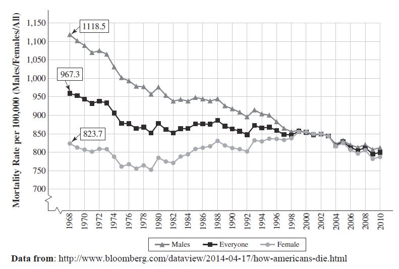
The mortality rate for the entire U.S. population in 1968 was 967.3 deaths per 100,000 people.
The mortality rate for U.S. women in 1968 was 823.7 deaths per 100,000 women. The mortality rate for U.S. men in 1968 was 1,118.5 deaths per 100,000 men.
Note the second quantity of this ratio is not always people! If it was you could add the male and female rates to get the total. Also note the 967.3 is not the average of the male and female rates, there are more women in the population so the overall rate skews towards the female rate.
2. They tell us the overall rate “fell by about 17%” from 1968 to 2010, from 967.3 to 799.5.
a. Verify this and quantify the change for the rates for men and women in a similar fashion.

The total change is 799.5 – 967.3 = –167.8, divide this by the original 967.3 to get –17.3%.
The total change is 784.4 – 823.7 = –39.3, divide this by the original 823.7 to get –4.8% for women.
The total change is 812 – 1,118.5 = –306.5, divide this by the original 1,118.5 to get –27.4% for men.
b. Why can we compare the 1970 and 2010 statistics, even though the population has increased over this period?
Because we are using rates per 100,000 which take into the population sizes.
3. The slide associated with the first graph above says the decline in mortality rates stops in the mid 1990’s and second slide with the graph below attributes this to the aging of the population.
a. What is the logic behind this argument?
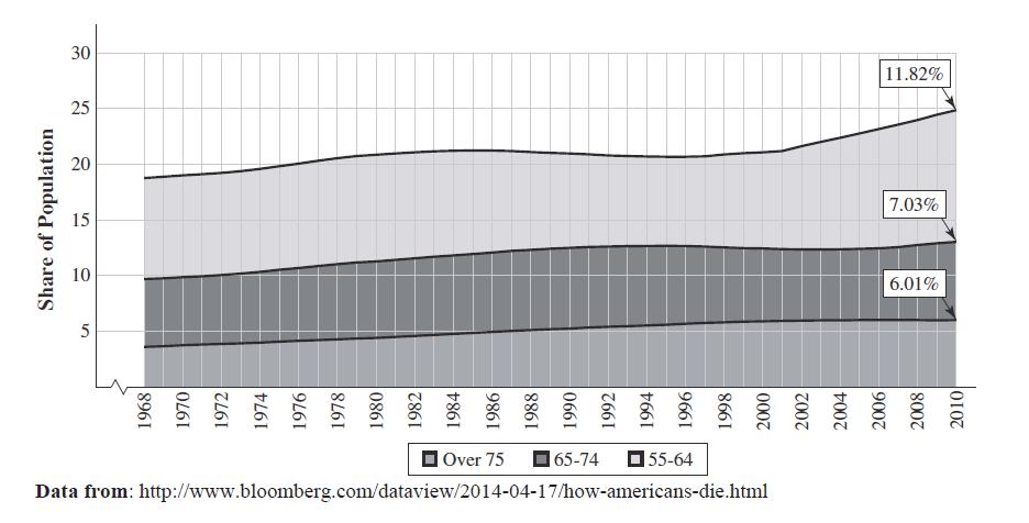
The aging population refers to a growing proportion of seniors in the population from 18.76% (from the slideshow but ~19%) 55 and older in 1968 to 24.86% (~25%) in 2010. So people living longer would first drive mortality rates down, but as we get a higher proportion of older people in the population, the mortality rates would stop dropping and level out as older people die sooner than younger people.
b. Interpret the 11.82% for 2010 in slide 2 and compare to the 25% on the vertical axis.
In 2010 11.82% of the population was in the 55 – 64 age bracket, and 25% of the population was 55 and older.
4. Looking at the graph below, which line stands out from the rest? What do you think accounts for this difference?

The 25–44 mortality rate line shoots up in the mid-1990’s. This was due to AIDS:
5. Interpret the statistics 80.16 and 64.03 for 1985 on graph in #4. Hint: Compare to the statistics shown here, and note that in 1968 the mortality rate for over 85 was 19,598.5 per 100,000 and the rate for below 25 was 160.7 per 100,000.

Looking at the 1985 statistics above in #5 we see a mortality rate of 15,710.8 deaths per 100,000 for over 85, and 102.9 deaths per 100,000 for under 25. The graph in #4 has set the rates for 1968 (19,598.5 and 160.7 respectively) equal to 100. The 80.16 in #4 comes from the proportion:
15,710.8 19,598.5100 x
Telling us that the rate for the over 85 group in 1985 is 80.16% of the 1968 rate. Similarly the rate for the under 25 group in 1985 is 64.03% of the 1968 rate.
6. Deaths from drugs in the 45 to 54 year old populations have increased by what factor from 1990 to 2010 as shown in this graph? Note the values for 1990 are set to 100.
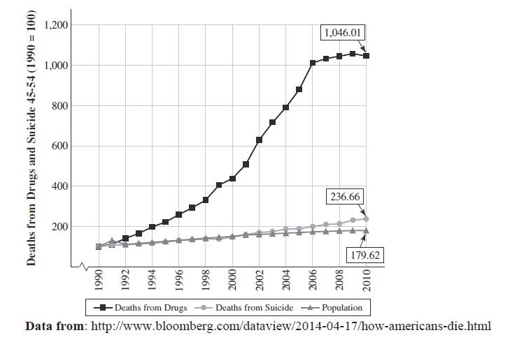
10.46 100 so a factor of 10.
7. Does this graph indicate Medicare spending has been increasing or decreasing since 2010?
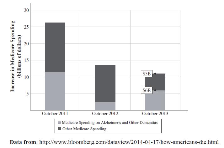
Medicare spending has been increasing, the increase has been decreasing. Look at the vertical axis it is “Increase in spending” not “spending”!
Chapter 1 – An Excel-lent Approach to Relationships
Section 1.1 Functions
Objective 1 – Learn Function Basics
Objective 2 – Explore Financial Functions
Objective 1 – Learn Function Basics
Guided Practice Activity #1 – Reasoning About Functions
1. The annual cost of a car is a function of many inputs. List all of the inputs you can think of that determine the output of the annual car cost.
gas, insurance, repairs, etc.
2. Determine which of the following are functions:
INPUTS OUTPUT FUNCTION?
States Senators No, 2 senators (outputs) per state (input).
Senators States Yes, each senator (input) has 1 and only 1 state (output).
States Number of senators Yes, constant function each state (input) has same output (2).
People
Anyone they been married to… No, the output will be multiple people for some inputs.
People Number of spouses Yes, the output is a single number for each person.
3. Come up with a function between two quantities which remains a function when you switch the inputs and outputs…
Input: Number of gallons of water
Output: Weight of the water
Excel Preview – 1.1 Heart Rate
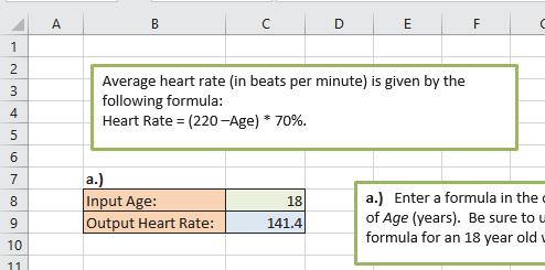
1. What formula would you type into cell C9?
=(220 – C8)*70%
2. According to this formula heart rate is a function of what input?
age
3. What are the units for the inputs and outputs for this function?
age: years
heart rate: BPM (beats per minute)
4. To make the following column chart how to we get the category x-axis labels to appear?
use Select Data and highlight the ages


Objective 2 – Explore Financial Functions
Guided Practice Activity #2 – Periodic Rates
For each of the following situations determine the periodic rate (four decimal places of accuracy), and the amount of interest charged in the first period. Creating a spreadsheet to do this will greatly speed up your work!
1. Balance = $576 APR = 8% weekly
a. Weekly rate? 0.1538%
b. First week’s interest? $0.89
2. Balance = $1396 APR = 3.5% daily
a. Daily rate? 0.0096%
b. First day’s interest? $0.13
3. Balance = $18,500 APR = 14% monthly
a. Monthly rate? 1.1667%
b. First month’s interest? $215.83
4. Balance = $18,500 APR = 1% monthly a. Monthly rate? 0.0833%
b. First month’s interest? $15.42
5. Balance = $450 APR = 240% monthly
a. Monthly rate? 20%
b. First month’s interest?
$90.00
Guided Practice Activity #3 – Financial Literacy: Credit Card Loan
Let us assume you buy a Sony flat screen TV for your dorm room that costs $1,000. You make the purchase with a store credit card that has a 12% Annual Percentage Rate (APR). You do not have to make any monthly payments for the first year (sounds good!), but they will charge interest at the end of each month. How much do you owe at the end of the first year?
1. What is the Principal?
$1,000
2. What is the monthly (periodic) interest rate? 1%
3. Monthly interest is a function of what two inputs?
APR and Balance
4. What is the interest charged for the first month?
$10


Double-click on the fill handle of the highlighted cells to quickly fill down to month 12 (you must have months 1-12 already filled in).

Cell Reference Handbook
Relative A4 Changes the row number when you fill up/down and changes the column letter when you fill left/right.
Mixed $A4 Changes the row number when you fill up/down and fixes the column letter when you fill left/right.
Mixed A$4 Fixes the row number when you fill up/down and changes the column letter when you fill left/right.
Absolute $A$4 Fixes the row number when you fill up/down and fixes the column letter when you fill left/right.
5. In the spreadsheet above, what formula is in cell C4? D4?
=B4*$G$6 and =B4+C4
6. Which formula involves an absolute cell reference?
=B4*$G$6
7. Why do we need to fill in the second row before we fill the formulas down?
To link the beginning of month 2 to the end of Month 1, which are the same value.
8. What do you owe at the end of the first year?
$1,126.83
9. What is the APY?

1. Assuming we now make a $50 payment, what formula is entered into cell E4?
=B4 + C4 – D4
2. What will the balance be at the start of month 2? $960
3. What formula is entered in cell B5? =E4
4. What formulas are entered in cells C5, D5, and E5?
=H$6*B5 =D4
=B5 + C5 – D5
5. Why do we need to fill in the formulas for month 2 before filling all of them down?
Need to connect beginning of month to end of previous month
6. Can we fill down all the formulas for month 2 together? How?
Yes! Highlight the entire row, grab the fill handle and pull down.
Section 1.2 Analytic Representatives: Equations
Objective 1 – Understand Order of Operations
Objective 2 – Evaluate Payment Function
Objective 1 – Understand Order of Operations
Guided Practice Activity #4 – Order of Operations
1. For each of the following compute using proper order of operations without a calculator.
a. 2–8/4+6*2 12
b. 3^2+1 10
c. 60/(2+8)-2^3*2 -10
d. 5+5/5+5 11
e. 12/6*4 8
2. Write down how you would type these into Excel as a formula:
a. 24 6 36 =(2+4)/(3*6)-6
b. 31 2 5 (84) =5+2/(8*4)^(3+1)
c. 46 92 1 811
=((9+2)/(8-11))^(4*6)-1
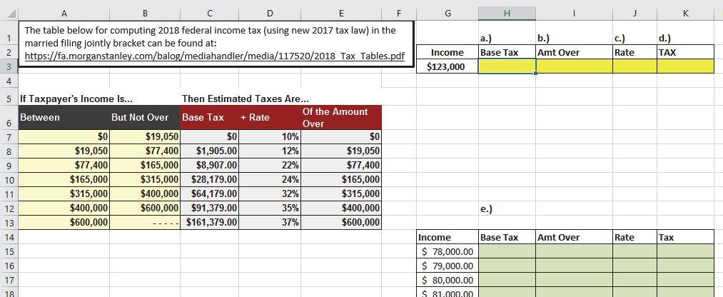
1. For a married couple filing jointly who make $123,000 in 2018 what is their base tax?
$8,907.00
2. How much more do they make than the “Of the Amount Over” value from column E for their row in the table?
$45,600
3. Compute their estimated taxes by adding the base tax and the correct percentage of the amount they make over the cutoff value. Note there is no division here! The word “over” implies “more than”.
$18,939
4. Are you surprised by how much they pay in taxes?
5. To make the following scatterplot chart what columns have been highlighted?
G and K
Federal Income Taxes for Filing Jointly Married
$30,000.00
$25,000.00
$20,000.00
$15,000.00
$10,000.00
$5,000.00
$-


Objective 2 – Evaluate Payment Function
Guided Practice Activity #5 – Payment Formula Using Order of Operations
You have just bought a new VW Jetta for $17,254.38. You put down $2,254.38 of your savings so you only have to borrow $15,000. The auto dealership gets you a loan from a bank for 5 years at 6%, which you agree to and sign. What will be your fixed monthly payment?
The periodic payment is a function of 4 inputs:
INPUTS
Principal (P)
OUTPUT
Periodic payment (PMT) APR
Number of periods in 1 year (n)
Number of years of the loan (t)
Use the following spreadsheet to answer the questions:

1. What is the term for this loan?
2. How many total payments will be made?
3. What will be the total amount paid?
4. What is the total amount interest paid?
$2,399.40
5. What formula is entered in cell E2? Does APR/n need its own parentheses?
=(A2*B2/C2)/(1-(1+B2/C2)^(-C2*D2)) NO!
Excel Preview – 1.6 BMI

1. What formula is typed into F6?
=C4*12 + C5
2. Are parentheses needed in this formula?
No
3. What formula is typed into cell F9?
=C8*0.45/(F6*0.025)^2
4. BMI is an index number and is meaningless without context. What else do we need to know in order to make sense out of the BMI computed in F9?
Range of values for possible BMI, with some sense of low and obese.
Section 1.3 Numerical and Graphical Representations: Tables and Charts
Objective 1 – Use Multiple Inputs to Understand What-If Analysis
Objective 2 – Convert Tables to Effective Graphs
Objective 1 – Use Multiple Inputs to Understand What-If Analysis
Guided Practice Activity #6 – Monthly Car Payments as Function of Two Inputs
You have just bought a new VW Jetta for $17,254.38. You put down $2,254.38 of your savings so you only have to borrow $15,000. The auto dealership gets you a loan from a bank for 5 years at 6%, which you agree to and sign. What will be your fixed monthly payment?
The periodic payment is a function of 4 inputs:
INPUTS OUTPUT
Principal (P)
APR
Number of periods in 1 year (n)
Number of years of the loan (t)
Periodic payment (PMT)
In the following spreadsheet we have already explored cell E2 that is a function of the four inputs in cells A2:D2. Now we will consider the two-way table in B6:H16, where we are holding the principal, �� = $15,000, fixed along with the number of months in one year, �� = 12. The monthly car payment becomes a function of two inputs: APR and term.

1. What are the two specific inputs, APR and term, for the highlighted payment of $456.33? 6% and 3 years
2. What formula is entered in cell C7 that will allow us to fill down and across? Note you may use the number 12 in your formula instead of the cell reference C2 since this is constant for monthly payments. In particular pay attention to what cell references are absolute, relative and mixed.
3. How much total interest is paid with the $289.99 monthly payment?
$2,399.40 = 5*12*$289.99 - $15,000 Note using values from spreadsheet gives slightly different answer: $2,399.52
4. How much would you save in interest if you switched your 5 year 6% loan to 3 years at 6%?
$971.52 = $2,399.40 – (3*12*$456.33 - $15,000)
5. What if you have a horrible credit score you might be forced to take out a 6 year loan at 10%. How much interest do you pay over the life of this loan?
$5,008.08 = 6*12*$277.89 - $15,000
6. What is fixed (column or row) by the following cell references?
Both Row Neither Both Row Column
Objective 2 – Convert Tables to Effective Graphs
Guided Practice Activity #7 – Effective Charts of Two Way Tables
To make an effective chart of a two way table we often simply highlight one column of data and then add appropriate labels. Let’s assume we want to make a chart showing the monthly payments a 5 year loan of $15,000 as a function of the different APR’s.

1. What cell range should you highlight for this chart?
G7:G16
2. The following chart does not have correct x-axis labels. How do you get the APR’s to show up on the �� -axis?
Click on Select Data and then edit Horizontal Category Axis Labels by selecting cells B7:B16.
3. How do you add axis titles and the chart title? Add Chart Element
4. How do you make the columns wider?
Right click on a column and choose Format Data Series and set gap Width to 5% or so
5. How do you make the vertical axis start at $250 to accentuate the difference in monthly payments?
Right click on vertical axis number and select Format Axis, set Minimum to 250
Monthly Payments for a 5 year Term
Excel Preview – 1.10 Wind Chill
The following screenshot gives the formula for Wind Chill.
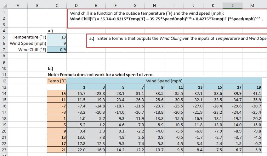
1. In cell D14 what are the inputs for the output of -15.7 degrees?
–15 degrees and 1 mph
2. What formula is in cell D14 that you can fill down and across? Pay attention to what should be a relative versus absolute or mixed cell reference.
Wind Chill(◦F) = 35.74+0.6215*Temp(◦F) – 35.75*Speed(mph)0.16 + 0.4275*Temp(◦F )*Speed(mph)0.16
=35.74+0.6215*$C14-35.75*D$13^0.16+0.4275*$C14*D$13^0.16
3. What cell range was highlighted to make the following line chart?
D21:M21
Wind Chills (◦F) for Temperature 13◦F
Wind Chills (◦F) Wind Speed (mph)
4. What cell range was highlighted to make the following surface chart?
C13:M23
Wind Chills (◦F)

135791113151719
Excel Preview – 1.6 BMI
BMI is calculated using the formula:

1. What formula would you type into cell C24 that can be filled down and across?
2. What cell range would be highlighted to make the following chart?
for 115 lbs.
Section 1.4 Spotlight on Statistics
Objective 1 – Learn Descriptive Statistics
Objective 2 – Compute Weighted Averages
Objective 3 – Create Histograms
Objective 1 – Learn Descriptive Statistics
Guided Practice Activity #8 – Age Distribution
The table and chart give the distribution of ages in the U.S. in 2016.
0
50 -- 59 21,413,590 22,405,574
60
1. What are the heights of the columns for the first bin in which women outnumber men? What do these heights represent? 20,152,276
2. The text indicates the median age is about 38 years old. What does this mean?
Half the population is younger than 38 and half older
3. Compute the number of people from 0 – 39 and 40 and above. Are these close to being equal?
169,937,244 under 40 and 153,190,269 over, yes close!
