

1.1 Functions from the Numerical, Algebraic, and Graphical Viewpoints
1. Based on the following table, find
a. 0.3
b. 1.45
c. 4
d. 3
e. 1
ANSWER: c
2. Based on the following table, find =

ANSWER: 2
3. Based on the following table, find .
a. 17
b. –1
c. 6
d. 11
e. 4
ANSWER: b
4. Based on the following table, find .
a. 6
b. 8
c. 6.6
d. 9
e. 7.4
ANSWER: a
5. Use the graph of the function to find
Copyright Cengage Learning. Powered by Cognero.
1.1 Functions from the Numerical, Algebraic, and Graphical Viewpoints
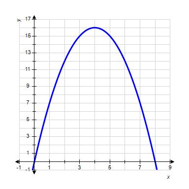
a. 11
b. 9
c. 16
d. 12
e. 14
ANSWER: d
6. Use the graph of the function f to find .
Copyright Cengage Learning. Powered by Cognero.
1.1 Functions from the Numerical, Algebraic, and Graphical Viewpoints
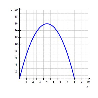
a. 10
b. 7
c. 5
d. 3
e. 6
ANSWER: b
7. Use the graph of the function to find
Copyright Cengage Learning. Powered by Cognero.
1.1 Functions from the Numerical, Algebraic, and Graphical Viewpoints
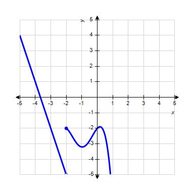
a. –1
b. –3
c. –4
d. –2
e. –3.5
ANSWER: d
8. Use the graph of the function f to find
Copyright Cengage Learning. Powered by Cognero.
1.1 Functions from the Numerical, Algebraic, and Graphical Viewpoints
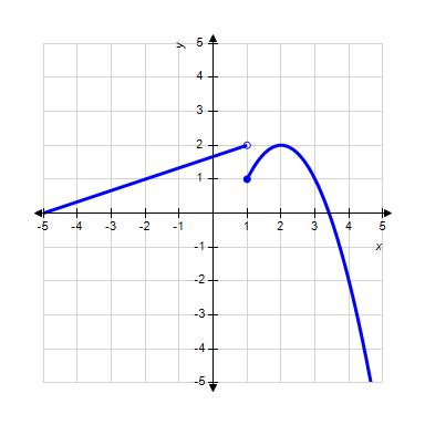
a. 1
b. –1
c. 2
d. 2.5
e. 3
ANSWER: a

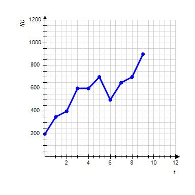
9. The graph shows the number of sports utility vehicles sold in the United States, where represents sales in year t in thousands of vehicles. Find .

Copyright Cengage Learning. Powered by Cognero.
1.1 Functions from the Numerical, Algebraic, and Graphical Viewpoints
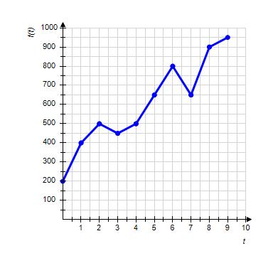
a. 450,000 vehicles
b. 500,000 vehicles
c. 800,000 vehicles
d. 400,000 vehicles
e. 650,000 vehicles
ANSWER: e
10. The graph shows the number of sports utility vehicles sold in the United States, where represents sales in year t in thousands of vehicles. Find .

Copyright Cengage Learning. Powered by Cognero.
1.1 Functions from the Numerical, Algebraic, and Graphical Viewpoints
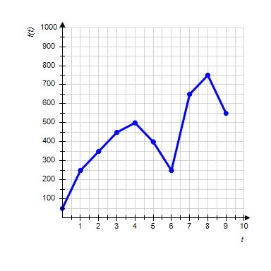
a. 450,000 vehicles
b. 250,000 vehicles
c. 400,000 vehicles
d. 550,000 vehicles
e. 500,000 vehicles
ANSWER: e
11. The graph shows the number of sports utility vehicles sold in the United States, where represents sales in year t in thousands of vehicles. Find .

Copyright Cengage Learning. Powered by Cognero.
1.1 Functions from the Numerical, Algebraic, and Graphical Viewpoints

a. 900,000 vehicles
b. 1,250,000 vehicles
c. 400,000 vehicles
d. 450,000 vehicles
e. 800,000 vehicles
ANSWER: a
12. The graph shows the number of sports utility vehicles sold in the United States, where represents sales in year t in thousands of vehicles. Find .
Copyright Cengage Learning. Powered by Cognero.
1.1 Functions from the Numerical, Algebraic, and Graphical Viewpoints
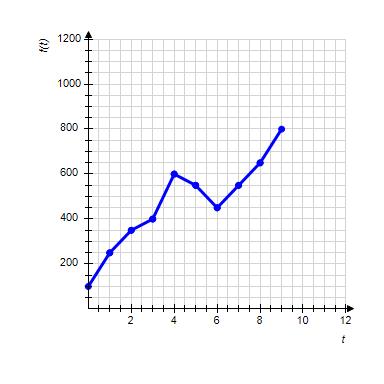
a. 400,000 vehicles
b. 600,000 vehicles
c. 550,000 vehicles
d. 450,000 vehicles
e. 800,000 vehicles
ANSWER: b
13. The graph shows the number of sports utility vehicles sold in the United States, where represents sales in year t in thousands of vehicles. Use the graph to estimate the largest value of for .
Copyright Cengage Learning. Powered by Cognero.
1.1 Functions from the Numerical, Algebraic, and Graphical Viewpoints

a. 700,000 vehicles
b. 450,000 vehicles
c. 950,000 vehicles
d. 600,000 vehicles
e. 400,000 vehicles
ANSWER: d
14. The graph shows the number of sports utility vehicles sold in the United States, where represents sales in year t in thousands of vehicles. Use the graph to estimate the largest value of for .
Copyright Cengage Learning. Powered by Cognero.
1.1 Functions from the Numerical, Algebraic, and Graphical Viewpoints
vehicles
ANSWER: 700,000

15. The graph shows the number of sports utility vehicles sold in the United States, where represents sales in year t in thousands of vehicles. Use the graph to estimate the smallest value of for
Copyright Cengage Learning. Powered by Cognero.
1.1 Functions from the Numerical, Algebraic, and Graphical Viewpoints

a. 250,000 vehicles
b. 400,000 vehicles
c. 700,000 vehicles
d. 550,000 vehicles
e. 450,000 vehicles
ANSWER: a
16. The graph shows the number of sports utility vehicles sold in the United States, where represents sales in year t in thousands of vehicles. Use the graph to estimate the smallest value of for .
Copyright Cengage Learning. Powered by Cognero.
1.1 Functions from the Numerical, Algebraic, and Graphical Viewpoints
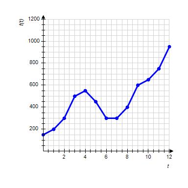
ANSWER: 300,000

17. Given , find .
a. 16
b. –4

c. d. 8
e. 4
ANSWER: e

18. Given , find


ANSWER: 7
19. Given , find .
a. 25
b. 15
c. –25
d. –5
Copyright Cengage Learning. Powered by Cognero.
Name: Class:
e. 5
ANSWER: c

20. Given , find .

ANSWER: –29
21. Given , find a. 4
b. 22
c. 16
d. 19
e. –4
ANSWER: b
22. Given , find
ANSWER: –5

23. Given , find .
a. 5
b. –3
c. 4
d. 3
e. 8
ANSWER: a


ANSWER: 7

24. Given , find .
25. Given , find .
1.1 Functions from the Numerical, Algebraic, and Graphical Viewpoints Copyright Cengage Learning. Powered by Cognero.
1.1 Functions from the Numerical, Algebraic, and Graphical Viewpoints
ANSWER: d

26. Given , find


ANSWER:

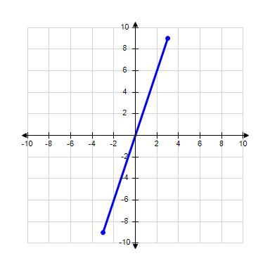
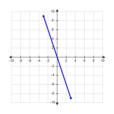
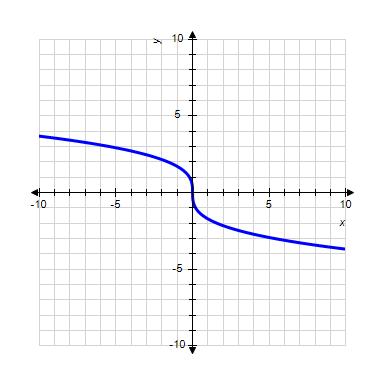
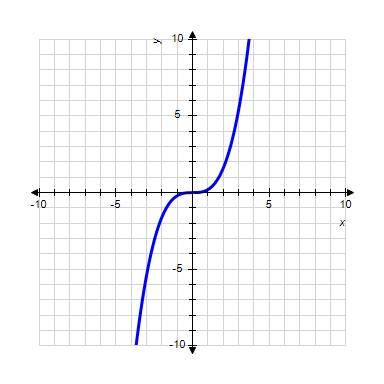
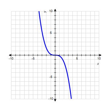
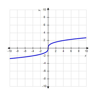
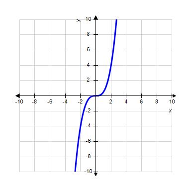
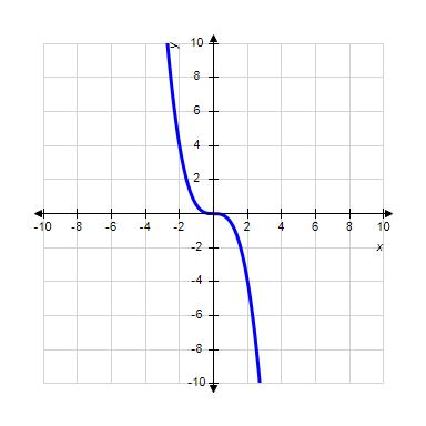
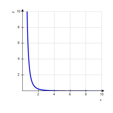
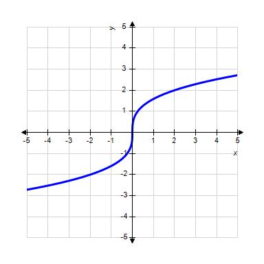
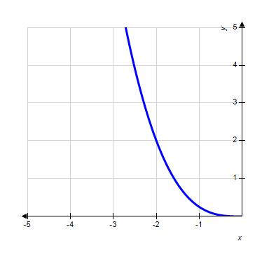
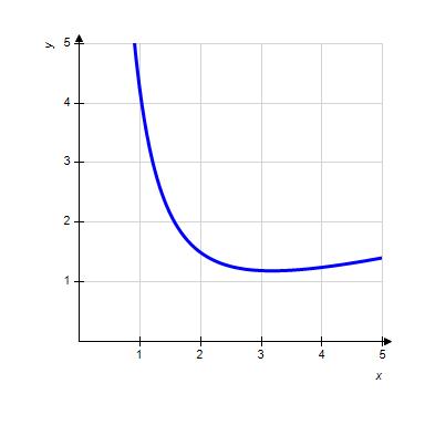
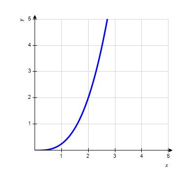
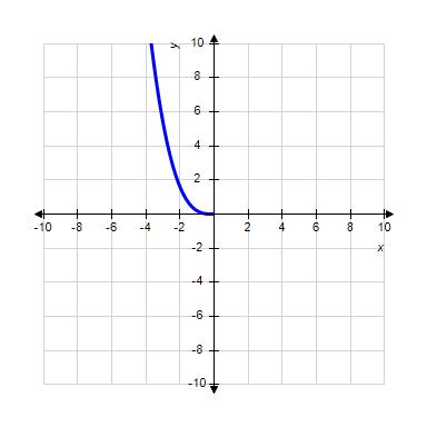
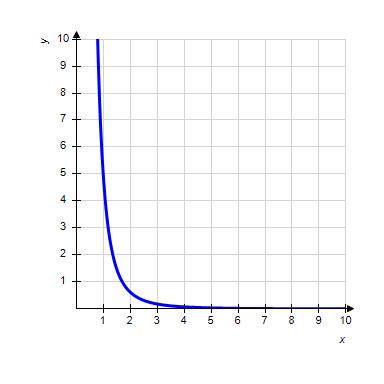
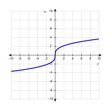
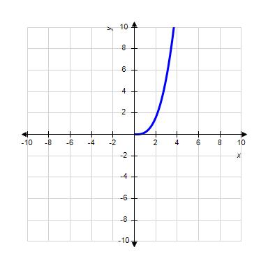
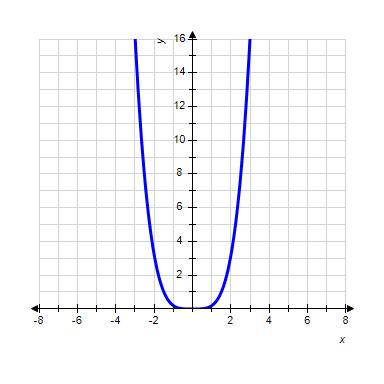
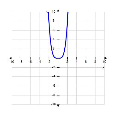
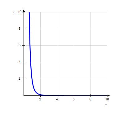
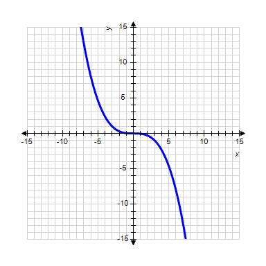
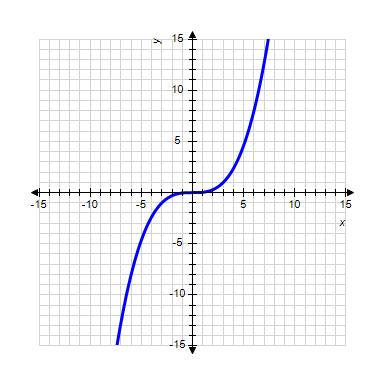
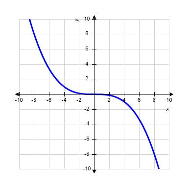
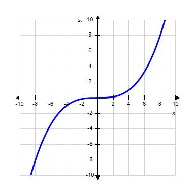
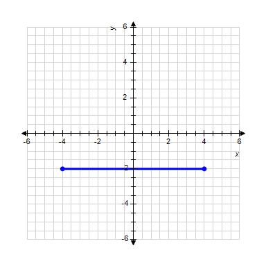
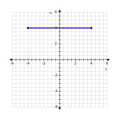
27. Choose the graph of the function , domain from the following:

Copyright Cengage Learning. Powered by Cognero.
1.1 Functions from the Numerical, Algebraic, and Graphical Viewpoints
ANSWER: c
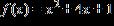
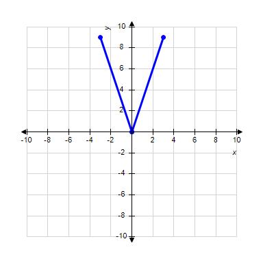
28. Graph the function over the domain [–3, 3].
Copyright Cengage Learning. Powered by Cognero.
1.1 Functions from the Numerical, Algebraic, and Graphical Viewpoints
ANSWER:
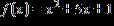
29. Graph the function over the domain [–3, 3].
Copyright Cengage Learning. Powered by Cognero.
1.1 Functions from the Numerical, Algebraic, and Graphical Viewpoints
ANSWER:
30. Graph the function over the domain [–3, 3].

Copyright Cengage Learning. Powered by Cognero.
1.1 Functions from the Numerical, Algebraic, and Graphical Viewpoints
ANSWER:


31. Choose the graph of the function , domain from the following:
Copyright Cengage Learning. Powered by Cognero.
1.1 Functions from the Numerical, Algebraic, and Graphical Viewpoints

ANSWER: d

Copyright Cengage Learning. Powered by Cognero.

32. Choose the graph of the function , domain from the following:
1.1 Functions from the Numerical, Algebraic, and Graphical Viewpoints
ANSWER: c
Copyright Cengage Learning. Powered by Cognero.
1.1 Functions from the Numerical, Algebraic, and Graphical Viewpoints

33. Choose the graph of the function , domain from the following:
Copyright Cengage Learning. Powered by Cognero.
1.1 Functions from the Numerical, Algebraic, and Graphical Viewpoints
ANSWER: d
34. Choose the graph of the function , domain from the following:

Copyright Cengage Learning. Powered by Cognero.
1.1 Functions from the Numerical, Algebraic, and Graphical Viewpoints
ANSWER: d

35. Choose the graph of the function , domain from the following:
Copyright Cengage Learning. Powered by Cognero.
1.1 Functions from the Numerical, Algebraic, and Graphical Viewpoints


ANSWER: d

Copyright Cengage Learning. Powered by Cognero.
36. Choose the graph of the function , domain from the following:
1.1 Functions from the Numerical, Algebraic, and Graphical Viewpoints
ANSWER: b


37. Choose the graph of the function , domain from the following:
Copyright Cengage Learning. Powered by Cognero.
1.1 Functions from the Numerical, Algebraic, and Graphical Viewpoints

ANSWER: d


Copyright Cengage Learning. Powered by Cognero.
38. Choose the graph of the function , domain from the following:
1.1 Functions from the Numerical, Algebraic, and Graphical Viewpoints

ANSWER: d
Copyright Cengage Learning. Powered by Cognero.

1.1 Functions from the Numerical, Algebraic, and Graphical Viewpoints
39. Use technology (such as spreadsheet, web site utilities, or a graphing calculator) to evaluate the function for
Round to three decimal places if necessary.
a. –23.475
b. –17.475
c. 27.525
d. –18.6
e. 21.525
ANSWER: b
40. Use technology (such as spreadsheet, web site utilities, or a graphing calculator) to evaluate the function for .

Round to four decimal places if necessary.
a. 1
b. 1.0405
c. 24.3000
d. 0.9611
e. 0.8684
ANSWER: d
41. Function is Find a. 32
b. 28
c. 30 d. 26
e. 6
ANSWER: e

42. Function f is . Find a. 115
Copyright Cengage Learning. Powered by Cognero.
1.1 Functions from the Numerical, Algebraic, and Graphical Viewpoints
b. 1
c. 120
d. 110
e. 125
ANSWER: b
43. Function f is

Find .
a. –7
b. –180
c. 7
d. –22
e. 22 ANSWER: b
44. Function is

Find
a. 63
b. –4
c. –67
d. –63
e. 30
ANSWER: b
45. Function f is .

Find .
a. –18
b. 81
c. 82
d. –81
e. No solution
ANSWER: b
Copyright Cengage Learning. Powered by Cognero.
1.1 Functions from the Numerical, Algebraic, and Graphical Viewpoints
46. Function is .
Find . a. 1,296
b. 6
c. 7
d. –6
e. No solution
ANSWER: b
47. Function f is
Find
a. 27
b. 26
c. 33
d. 40
e. 23
ANSWER: a
48. Function is .
Find .
a. 162
b. 168
c. 36
d. 27
e. 174
ANSWER: a

49. The value of U.S. trade with China from 1994 through 2002 could be approximated by billion dollars, where t is time in years since 1994.
Find an appropriate domain of C
a.
Copyright Cengage Learning. Powered by Cognero.
1.1 Functions from the Numerical, Algebraic, and Graphical Viewpoints


e.
ANSWER: d
50. The number of research articles in a professional journal that were written by researchers in the U.S. from 1983 through 2002 could be approximated by articles, where t is time in years since 1983.
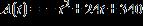
Find an appropriate domain of A.
a.

b.
c.
d.
e.

ANSWER: a
51. The processor speed, P(t), in megahertz, of computer processors was able to be modeled by the function of time t in years since the start of 1995:
Use the model and a table of values to estimate when processor speeds first hit 3.2 gigahertz (1 gigahertz = 1,000 megahertz).
a. years
b. years
c. years
d. years
e. years
ANSWER: d
52. The value of the Conference Board Index of 10 economic indicators in the U.S., E(t), was approximated by the function of time t in months from the end of December 2002:
Use the model and a table of values to estimate when the index was 113, prior to March 2004.
a. months
Copyright Cengage Learning. Powered by Cognero.
1.1 Functions from the Numerical, Algebraic, and Graphical Viewpoints
b. months
c. months
d. months
e. months
ANSWER: b

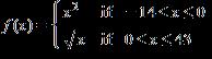
53. The percentage of children who are able to speak in at least single words by the age of t months can be approximated by the equation:
Use a table of values to determine what percent of children are able to speak in at least single words by the age of 14 months. Round to the nearest percent.
a. 73%
b. 86%
c. 61%
d. 79%
e. 14%
ANSWER: b
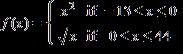
54. The percentage of children who are able to speak in at least single words by the age of t months can be approximated by the equation.
Use a table of values to determine by what age are 80% of children speaking in at least single words. Round to the nearest month.
a. 15
b. 6
c. 10
d. 4
e. 7
ANSWER: c
55. If the revenue R is specified as a function of time t, which variable is independent?
a. R
b. t
c. Neither variable
d. Both variables
ANSWER: b
Copyright Cengage Learning. Powered by Cognero.
1.1 Functions from the Numerical, Algebraic, and Graphical Viewpoints
56. If the income I is specified as a function of selling price s, which variable is independent, and which one is dependent?
Dependent:_______ Independent:
ANSWER: I; s
57. Write the equation using function notation.


ANSWER: b
Copyright Cengage Learning. Powered by Cognero.
1.2 Functions and Models
1. The following table shows the approximate value V of one Euro in U.S dollars from its introduction in January 2003 to January 2006, where represents January, 2003.
Year, t 3 5 6
Which model would best fit the given data? (A, a, b, c, k, l, and m are constants.)
a. Logarithmic:

b. Cubic:

c. Linear:

d. Quadratic:
e. Exponential:

ANSWER: d
2. The following table shows the approximate average household income in the U.S. for three different years.
Year, t 0 5 13
Household Income in $1000, H 30 35 43
Which of the following kinds of models would best fit the given data? (A, a, b, c, and m are constants.)
a. Exponential:
b. Logarithmic:
c. Linear:
d. Quadratic:
e. Power:
ANSWER: c
3. A teenager bought an ice cream cart for $697 that they will push each day to sell ice creams. If each ice cream costs $1.50, write the cost function for their ice cream business, where x is the number of ice creams that teenager buys to stock the cart.
a. C(x) = 697 – 1.50x
b. C(x) = 697 + 1.50x
c. C(x) = 697x + 1.50
d. C(x) = 697x – 1.50
e. C(x) = 698.5x
ANSWER: b
4. The purchase and initial set up of a coffee cart is $534. The cost to produce a cup of coffee is $1.25. Find the total cost of the cart if 33 cups of coffee are produced.
1.2 Functions and Models
ANSWER: 575.25
5. The cost function for the XYA company to produce Xbots is given by . The company can sell each Xbot for $182. Write the profit function P(x), where x is the number of Xbots that are produced and sold.
a.
b. c.
d.
e.
ANSWER: a
6. A teenager bought an ice cream cart for $354 that they will push each day to sell ice creams. If each ice cream costs $0.75, and the teenager sells each ice cream for $4.5, write the profit function P when x is the number of ice creams bought and sold.
P(x) =
ANSWER:
7. The cost function for the XYA company to produce x Xbots is given by The company can sell each Xbot for $209. Find the number of Xbots that the XYA company should produce and sell in order to break even. Round up to the nearest whole number as needed.
a. 20 Xbots
b. 21 Xbots
c. 13 Xbots
d. 14 Xbots
e. No breakeven point
ANSWER: b
8. The cost function for the Coral company to produce x coral necklaces is given by dollars. The company can sell each coral necklace for $7.25. Find the number of coral necklaces that the company needs to produce and sell in order to break even. Round up to the nearest whole number, as needed.
___________coral necklaces
ANSWER: 105
9. The Oliver company plans to produce and sell a new product. Based on its market studies, Oliver estimates that it can sell up to 7,000 units. The selling price will be $3 per unit. Variable costs are estimated to be 20% of total revenue. Fixed costs are estimated to be $15,600. How many units should the company sell to break even?
a. 7,000 units
b. 15,600 units
c. 4,333 units
1.2 Functions and Models
d. 6,500 units
e. 5,200 units
ANSWER: d
10. The Oliver company plans to produce and sell a new product. Based on its market studies, Oliver estimates that it can sell up to 6,500 units. The selling price will be $1 per unit. Variable costs are estimated to be 35% of total revenue. Fixed costs are estimated to be $3,900. How many units should the company sell to break even?
Number of units =
ANSWER: 6,000
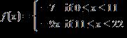
11. The demand, as measured by total enrollment, for a private daycare downtown can be modeled by students enrolled, where 11 ≤ p ≤ 36 and p is the daily net tuition in dollars. Find the number of students who could attend the daycare if the daily tuition rate is $16.
a. 63 students
b. 11 students
c. 57 students
d. 16 students
e. 36 students
ANSWER: a
12. The demand, as measured by total enrollment, for a private daycare downtown can be modeled by students enrolled, where 10 ≤ p ≤ 41 and p is the daily net tuition in dollars. Based on this demand equation, could 71 students attend the daycare? If so, what is the tuition per student per day? If not, why not?
a. Yes and the daily tuition would be $4.33 per student per day.
b. Yes, and the daily tuition would be $45.33 per student per day.

c. No, since if , the tuition (p) would be approximately $4.33, which is not within the domain set for p
d. No, since if , the tuition (p) would be approximately $45.33, which is not within the domain set for p
e. Not enough information is given to determine whether 71 students could attend or not.
ANSWER: c
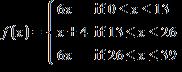
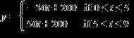
13. The demand, as measured by total enrollment, for a private daycare downtown can be modeled by

students enrolled, where 10 ≤ p ≤ 36 and p is the daily net tuition in dollars. The daycare will create space for students, who pay the daily net tuition rate of p dollars, with 10 ≤ p ≤ 36. What is the equilibrium daily tuition at the daycare? Round to the nearest hundredth, as needed.
a. $33.17
b. $36.00
c. $36.77
d. $10.00
1.2 Functions and Models
e. There is no equilibrium daily tuition in that range.
ANSWER: a

14. The demand, as measured by total enrollment, for a private daycare downtown can be modeled by students enrolled, where 9 ≤ p ≤ 44 and p is the daily net tuition in dollars. The daycare will create space for students, who pay the daily net tuition rate of p dollars, with 9 ≤ p ≤ 44. What is the equilibrium daily tuition at the daycare? Round to the nearest hundredth, as needed.
$_______
ANSWER: 29.73


15. If with domain and with domain , find r(0) if .
a.
b.


c. 0
d. r(0) does not exist
e.

ANSWER: b

16. If with domain (–∞, 10] and with domain (–∞, ∞), find and the domain of s If the function does not exist, write DNE.
s(x) = Domain: _____________(use interval notation)
ANSWER:

1.3 Linear Functions and Models
1. A table of values for a linear function is given. Find x 2 3 f(x) –2 –9
ANSWER: c
2. A table of values for a linear function is given. Find x –1 0 f(x)


ANSWER: e
3. A linear function is given by the table. Find
ANSWER: e
4. A linear function is given by the table. Find
= ANSWER: 5
1.3 Linear Functions and Models
5. Find the equation of the given linear function.
ANSWER: b
6. Find the equation of the given linear function. x
Enter your answer as an equation of a linear function, .
ANSWER:
7. Decide which of the two given functions is linear and find its equation.
ANSWER: e
8. Decide which of the two given functions is linear and find its equation.
Which of the two functions is linear? ____________(f /g)
Write the equation of the linear function, using ANSWER:

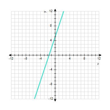
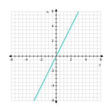
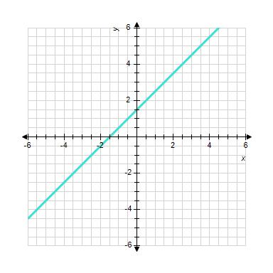
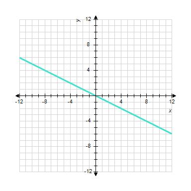
9. Sketch the straight line of the following equation.


1.3 Linear Functions and Models
ANSWER: c
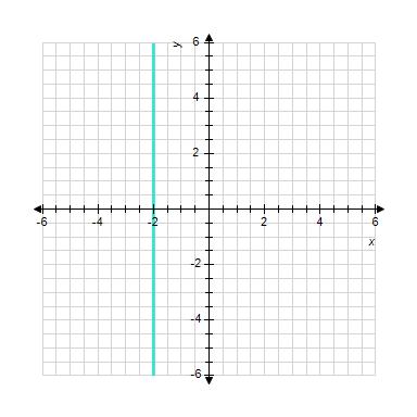
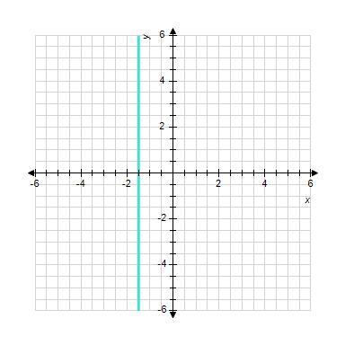
10. Sketch the straight line with the equation.

1.3 Linear Functions and Models

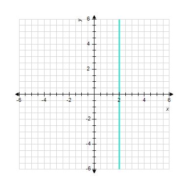
ANSWER: e
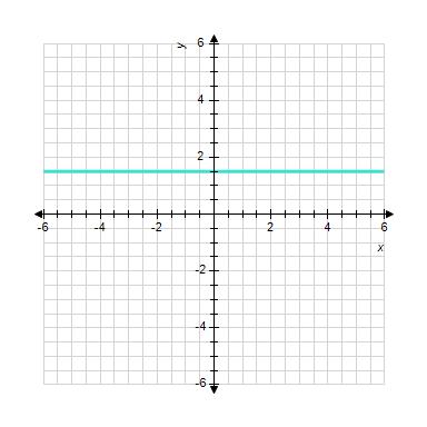
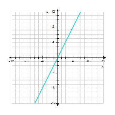
11. Sketch the straight line with the equation.
1.3 Linear Functions and Models

ANSWER: a
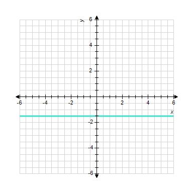
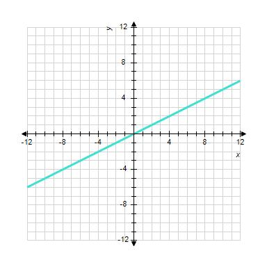
12. Sketch the straight line with the equation.

1.3 Linear Functions and Models
ANSWER: b
13. Calculate the slope of the straight line through the points (4, 3) and (9, 13).
a. b. c. d.
e.


ANSWER: e
14. Calculate the slope of the straight line through the points (4, 4) and (7, 1).
ANSWER: –1


15. Calculate the slope of the straight line through the points and . a. b. c.

1.3 Linear Functions and Models

ANSWER: e
16. Calculate the slope of the straight line through the points (2.3, 1) and (7.3, 11).
ANSWER: 2
17. Calculate the slope of the straight line through the points and


ANSWER: a


18. Calculate the slope of the straight line through the points and
ANSWER: 2
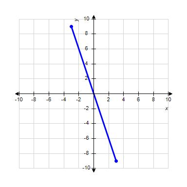
19. Estimate the slope of the line segment.

Linear Functions and Models
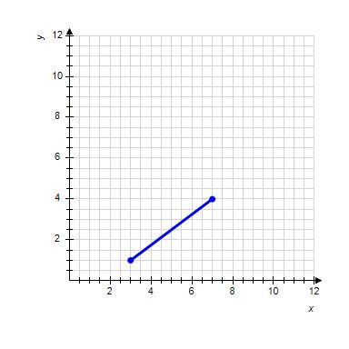


e. ANSWER: d
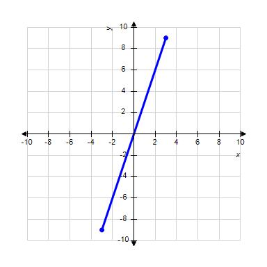
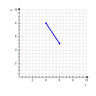
20. Estimate the slope of the line segment.
1.3 Linear Functions and Models

Enter your answer as a fraction if necessary.
ANSWER:
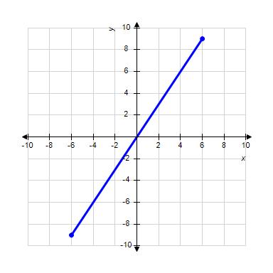
21. Estimate the slope of the line segment.
1.3 Linear Functions and Models
Enter your answer as a fraction if necessary.
ANSWER:

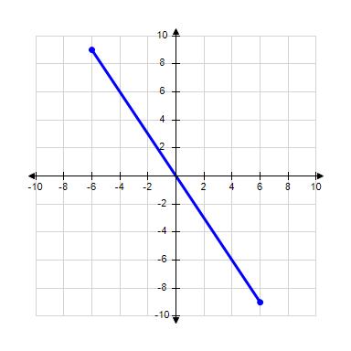
22. Estimate the slope of the line segment.
1.3 Linear Functions and Models
a. b. c. d.
e. Undefined
ANSWER: a
23. Estimate the slope of the line segment.
1.3 Linear Functions and Models
Enter your answer as a fraction if necessary.
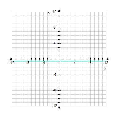
ANSWER: 0

24. Find the linear equation for the straight line through with slope 4. a. b. c. d. e.
ANSWER: e
25. Find the linear equation for the straight line through (2, 5) with slope 4.
Enter your answer as an equation in the form
ANSWER:

26. Find the linear equation for the straight line through with slope . a.

1.3 Linear Functions and Models


ANSWER: a
27. Find the linear equation for the straight line through with slope .

Enter your answer as an equation in the form .
ANSWER:

28. Find the linear equation for the straight line through (23, –2.4) that increases at a rate of 10 units of y per unit of x.
ANSWER: c
29. Find the linear equation for the straight line through (21, –2.6) that increases at a rate of 15 units of y per unit of x.
Enter your answer as an equation in the form .
ANSWER:
30. Find the linear equation for the straight line through (4, 4) and (7, 22). a.
e.
ANSWER: e
1.3 Linear Functions and Models
31. Find the linear equation for the straight line through (1, 3) and (6, 23).
Enter your answer as an equation in the form .
ANSWER:
32. Find the linear equation for the straight line through (6, 8) that is parallel to the line . a. b. c. d.
e.
ANSWER: e
33. Find the linear equation for the straight line through (5, 8) that is parallel to the line .
Enter your answer as an equation in the form .
ANSWER:
34. A piano manufacturer has a daily fixed cost of $1,600 and a marginal cost of $2,100 per piano. On a given day, what is the cost of manufacturing 4 pianos?
a. $6,800
b. $14,800
c. $6,800
d. $10,000
e. $8,500
ANSWER: d
35. A piano manufacturer has a daily fixed cost of $1,100 and a marginal cost of $1,600 per piano. On a given day, what is the cost of manufacturing 4 pianos?
$ ANSWER: 7,500
36. A piano manufacturer has a daily fixed cost of $1,100 and a marginal cost of $1,600 per piano. Find the cost C of manufacturing x pianos in one day.
a. per day
b. per day
c. per day
d. per day
1.3 Linear Functions and Models
e. per day
ANSWER: e
37. A piano manufacturer has a daily fixed cost of $1,200 and a marginal cost of $1,700 per piano. Write the equation for the cost c of manufacturing x pianos in one day.
ANSWER:
38. You can sell 80 pet chias per week if they are marked as $2 each, but only 30 per week if they are marked $3 per chia. Your chia supplier is prepared to sell you 10 chias per week if they are marked $2 per chia, and 60 per week if they are marked $3 per chia. Write the associated linear demand and supply functions.
a. ,
b. ,
c. ,
d. ,
e. ,
ANSWER: c
39. You can sell 75 pet chias per week if they are marked as $5 each, but only 25 per week if they are marked $6 per chia. Your chia supplier is prepared to sell you 10 chias per week if they are marked $5 per chia, and 60 per week if they are marked $6 per chia. Write the associated linear demand and supply functions, using the notation: q for demand, s for supply, and p for price.
Demand:
Supply:
ANSWER: ,
40. You can sell 85 pet chias per week if they are marked as $1 each, but only 35 per week if they are marked $2 per chia. Your chia supplier is prepared to sell you 20 chias per week if they are marked $1 per chia, and 70 per week if they are marked $2 per chia. At what price should the chias be marked so that there is neither surplus nor a shortage of chias?
a. $1.65
b. $1.79
c. $1.46
d. $1.70
e. $2.05
ANSWER: a
41. You can sell 55 pet chias per week if they are marked as $1 each, but only 45 per week if they are marked $2 per chia. Your chia supplier is prepared to sell you 25 chias per week if they are marked $1 per chia, and 35 per week if they are marked $2 per chia. At what price should the chias be marked so that there is neither surplus nor a shortage of chias? Round your answer to two decimal places.
$ ANSWER: 2.50
1.3 Linear Functions and Models
42. The demand for your college newspaper is 1600 copies per week if the paper is given away free of charge, and the demand drops to 800 if the charge is $0.25 per copy. However, the university is prepared to supply only 400 copies per week free of charge but will supply 3800 per week at $0.50 per copy. At what price should the college newspapers be sold so that there is neither a surplus nor a shortage of papers?
a. $0.10
b. $0.06
c. $0.24
d. $0.18
e. $0.12
ANSWER: e
43. The demand for your college newspaper is 1,000 copies per week if the paper is given away free of charge, and the demand drops to 500 if the charge is $0.10 per copy. However, the university is prepared to supply only 400 copies per week free of charge but will supply 1,650 per week at $0.25 per copy. At what price should the college newspapers be sold so that there is neither a surplus nor a shortage of papers? Round your answer to two decimal places.
$ ANSWER: 0.06
44. Annual federal spending on Medicare increased more or less linearly from $65 billion in 1973 to $107 billion in 1994. Use these data to express s, the annual spending on Medicare (in billions of dollars), as a linear function of t, the number of years since 1973.
a.
b.
c.
d.
e.
ANSWER: e
45. Annual federal spending on Medicare increased more or less linearly from $60 billion in 1980 to $144 billion in 1999. Use these data to express s, the annual spending on Medicare (in billions of dollars), as a linear function of t, the number of years since 1980. Express the equation in form.
ANSWER:

46. U.S. imports of pasta increased from 290 million pounds in 1990 , by an average of 52 million pounds per year. Estimate U.S. pasta import (in million pounds) in the year 2000, assuming the import trend continued.
a. 2,290 million pounds
b. 862 million pounds
c. 342 million pounds
d. 520 million pounds
e. 810 million pounds
1.3 Linear Functions and Models
ANSWER: e
47. U.S. imports of pasta increased from 290 million pounds in 1990 (t = 0), by an average of 52 million pounds per year. Estimate U.S. pasta import (in million pounds) in the year 1995, assuming the import trend continued.
million pounds
ANSWER: 550
48. The position of a model train, in feet along the railroad track, is given by after t seconds.
Where is the train after 10 seconds?
a. 18 feet
b. 43 feet
c. 21.5 feet
d. 115 feet
e. 35 feet
ANSWER: b
49. The position of a model train, in feet along the railroad track, is given by after t seconds. Where is the train after 10 seconds?
feet
ANSWER: 45
50. The position of a model train, in feet along the railroad track, is given by after t seconds.
When will the train have moved a distance of 21 feet?
a. after 6 seconds
b. after 2 seconds
c. after 17 seconds
d. after 12 seconds
e. after 7 seconds
ANSWER: b
51. The position of a model train, in feet along the railroad track, is given by after t seconds.
When will the train have moved a distance of 27 feet?
t = seconds
ANSWER: 8

52. The height of the falling sheet of paper, in feet from the ground, is given by after t seconds. When will the sheet of paper reach the ground?
a. after 12 seconds
1.3 Linear Functions and Models
b. after 9 seconds
c. after 16 seconds
d. after 4 seconds
e. after 2 seconds
ANSWER: d
53. The height of the falling sheet of paper, in feet from the ground, is given by after t seconds. When will the sheet of paper reach the ground?
seconds
ANSWER: 12
54. A police car was traveling down Ocean Parkway in a high-speed chase from Jones Beach. The car was at Jones Beach at exactly 7:00 p.m. , and was at Oak Beach, 13 miles from Jones Beach, at exactly 7:05 p.m. How fast was the police car traveling? (Round your answer to the nearest tenth.)
a. 2.2 miles/min.
b. 3.3 miles/min.
c. 2.6 miles/min.
d. 2.0 miles/min.
e. 2.4 miles/min.
ANSWER: c
55. A police car was traveling down Ocean Parkway in a high-speed chase from Jones Beach. The car was at Jones Beach at exactly 9:00 p.m. , and was at Oak Beach, 13 miles from Jones Beach, at exactly 9:07 p.m. How fast, in miles per minute, was the police car traveling? Round your answer to one decimal place.
v =
ANSWER: 1.9

56. A car that was being pursued by the police was at Jones Beach at exactly 10:57 p.m. , and passed Oak Beach (13 miles from Jones Beach) at exactly 11:06 p.m.,where it was overtaken by the police. How fast, in miles per minute, was the car traveling? (Round your answer to the nearest tenth.)
a.


1.3 Linear Functions and Models
e.
ANSWER: d
57. A car that was being pursued by the police was at Jones Beach at exactly 9:57 p.m. , and passed Oak Beach (13 miles from Jones Beach) at exactly 10:04 p.m., where it was overtaken by the police. How fast, in miles per minute, was the car traveling?
Round your answer to the nearest tenth.
v = miles/minute
ANSWER: 1.9
58. In the Fahrenheit temperature scale, water freezes at 32°F and boils at 212°F. In the Celsius (or centigrade) scale, water freezes at 0°C and boils at 100°C. Assuming that the Fahrenheit temperature F and the Celsius temperature C are related by a linear equation, find the Fahrenheit temperature that correspond to 2°C, to the nearest degree.
a. 33°F
b. 61°F
c. 36°F
d. 4°F
e. 34°F
ANSWER: c
59. In the Fahrenheit temperature scale, water freezes at 32°F and boils at 212°F. In the Celsius (or centigrade) scale, water freezes at 0°C and boils at 100°C. Assuming that the Fahrenheit temperature F and the Celsius temperature C are related by a linear equation, find the Celsius temperature that correspond to 147°F, to the nearest degree.
a. 114°C
b. 115°C
c. 64°C
d. 99°C
e. 233°C
ANSWER: c
60. In the Fahrenheit temperature scale, water freezes at 32°F and boils at 212°F. In the Celsius (or centigrade) scale, water freezes at 0°C and boils at 100°C. Assuming that the Fahrenheit temperature F and the Celsius temperature C are related by a linear equation, find the Fahrenheit temperature that corresponds to 40°C, to the nearest degree.
°F
ANSWER: 104
61. In the Fahrenheit temperature scale, water freezes at 32°F and boils at 212°F. In the Celsius (or centigrade) scale, water freezes at 0°C and boils at 100°C. Assuming that the Fahrenheit temperature F and the Celsius temperature C are related by a linear equation, find the Celsius temperature that correspond to 74°F, to the nearest degree.
°C
ANSWER: 23
1.3 Linear Functions and Models
62. The Snowtree cricket behaves in a rather interesting way: The rate at which it chirps depends linearly on the temperature. One summer evening you hear a cricket chirping at a rate of 140 chirps per minute, and you notice that the temperature is 80°F. Later in the evening, the cricket has slowed down to 120 chirps per minute, and you notice that the temperature has dropped to 75°F. What is the temperature if the cricket is chirping at a rate of 104 chirps per minute?
a. 71°F
b. 69°F
c. 77°F
d. 66°F
e. 75°F
ANSWER: a
63. The Snowtree cricket behaves in a rather interesting way: The rate at which it chirps depends linearly on the temperature. One summer evening you hear a cricket chirping at a rate of 140 chirps per minute, and you notice that the temperature is 80°F. Later in the evening, the cricket has slowed down to 120 chirps per minute, and you notice that the temperature has dropped to 75°F. What is the temperature if the cricket is chirping at a rate of 100 chirps per minute?
°F
ANSWER: 70
64. In a particular country the number of retirees was approximately 150 per thousand people aged 20-64 in the first year of keeping that data. Forty years later, this number rose to approximately 200, and it was projected to rise to 275 after 50 years. Model N as a piecewise linear function of the time t in years since the first year, letting t = 0 represent the first year of keeping data. Then use your model to project the number of retires per thousand people aged 20-64 in year 47. (Round your answer to the nearest integer.)
a. 208 people per thousand
b. 270 people per thousand
c. 249 people per thousand
d. 187 people per thousand
e. 145 people per thousand
ANSWER: a
65. In a particular country the number of retirees was approximately 150 per thousand people aged 20-64 in the first year of keeping that data. Forty years later, this number rose to approximately 200, and it was projected to rise to 275 after 50 years. Model N as a piecewise linear function of the time t in years since the first year, letting t = 0 represent the first year of keeping data. Then use your model to project the number of retirees per thousand people aged 20-64 in year 46.
Round your answer to the nearest integer.
retirees
ANSWER: 215
66. Following are some approximate values for a particular index.
Obtain a piecewise linear model of the index for to .
1.3 Linear Functions and Models


ANSWER: c
67. Following are some approximate values for a particular index.
t 0 5 9
(a) Model the data for and with a linear equation.
y =
(b) Model the data for and with a linear equation.
y =
(c) Use the results of parts (a) and (b) to obtain a piecewise linear model for the index values for

(d) Use your model to estimate the index when .
y =
ANSWER: ; ; ; 5; ; 5; 175
1.4 Linear Regression


1. Find the regression line associated with the set of points. , , a. b. c. d. e.
ANSWER: a
2. Find the regression line associated with the set of points. , , Enter the equation of the line in the form Round m and b to the nearest hundredth if necessary. ANSWER:


3. Find the regression line associated with the set of points. , , a. b.
ANSWER: c
4. Find the regression line associated with the set of points. , ,


Enter the equation of the line in the form . Round m and b to the nearest hundredth if necessary. ANSWER:


5. Find the regression line associated with the set of points. , , , a. b. c. d. e.
ANSWER: e
1.4 Linear Regression
6. Find the regression line associated with the set of points. , , ,


Enter the equation of the line in the form . Round m and b to the nearest hundredth if necessary.
ANSWER:
7. Find the regression line associated with the set of points. , , ,


ANSWER: d
8. Find the regression line associated with the set of points. , , ,


Enter the equation of the line in the form Round m and b to the nearest hundredth if necessary.
ANSWER:
9. Find the regression line associated with the set of points. Round all coefficients to 4 decimal places. , ,


ANSWER: e
10. Find the coefficient of correlation of the line that best fits the data set.

ANSWER: a
1.4 Linear Regression

11. Find the coefficient of correlation of the line that best fits the data set. a.
ANSWER: a

12. Find the coefficient of correlation of the line that best fits the data set. a. b.
ANSWER: b

13. Find the coefficient of correlation of the line that best fits the data set. a. b. c.
ANSWER: a
14. Find the coefficient of correlation of the line that best fits the data set.

e.
ANSWER: e
1.4 Linear Regression
15. Find the coefficient of correlation of the line that best fits the data set.

ANSWER: b
16. Find the coefficient of correlation of the line that best fits the data set.

Round the answer to four decimal places if necessary.
r = ANSWER: 0.9985
17. Find the coefficient of correlation of the line that best fits the data set.

Round the answer to four decimal places if necessary.
r = ANSWER: 1
18. Find the coefficient of correlation of the line that best fits the data set.

Round the answer to four decimal places if necessary.
r = ANSWER: 0.8486
19. Find the coefficient of correlation of the line that best fits the data set.

Round the answer to four decimal places if necessary.
r = ANSWER: –0.6628
20. Find the coefficient of correlation of the line that best fits the data set.

1.4 Linear Regression
Round the answer to four decimal places if necessary.
r = ANSWER: 0.5636
21. Find the coefficient of correlation of the line that best fits the data set.

Round the answer to four decimal places if necessary.
r = ANSWER: –1
22. Use correlation coefficients to determine which of the given sets of data is worst fit by its associated regression line.


a. I
b. II and III
c. III
d. I and II
e. II
ANSWER: e
23. a) Find the correlation coefficient associated with the regression line that best fits the set of data. Round the answer to 4 decimal places if necessary.
r =
b) Find the correlation coefficient associated with the regression line that best fits the set of data. Round the answer to 4 decimal places if necessary.

r =
c) Find the correlation coefficient associated with the regression line that best fits the set of data. Round the answer to 4 decimal places if necessary.

r =
Use the correlation coefficients to determine which of the given sets of data is best fit by its associated regression line.
(a, b, or c)
1.4 Linear Regression
Use the correlation coefficients to determine which of the given sets of data is worst fit by its associated regression line.
(a, b, or c)
Is it a perfect fit for any of the data sets?
(a, b, or c)
ANSWER: –1; 0; –0.9990; a; b; a
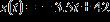
24. Some forecasts of worldwide annual cell phone sales are shown in the table:
Find the equation of the associated regression line, rounding coefficients to 2 decimal places if necessary. Then, use this regression line equation to project the sales in year 14.
a. 1308.33 million phones
b. 1298.33 million phones
c. 1328.33 million phones
d. 1320.33 million phones
e. 1290.33 million phones
ANSWER: a
25. The forecasts of worldwide annual cell phone sales are shown in the table:
a. Complete the table.
b. Find the equation of the associated regression line, rounding coefficients to 2 decimal places if necessary.
Slope: Intercept:
c. Use your regression line equation from part b to project the sales in year 17, rounding the answer to 2 decimal places if necessary.
million phones
ANSWER: 1500; 9; 3000; 25; 5600; 49; 15; 1900; 10100; 83; 75; 258.33; 1533.33
1.4 Linear Regression
26. Some approximate values of a particular index are shown in the table: Year, x 0 2 4 Index values, y 50
Find the equation of the associated regression line, rounding coefficients to 2 decimal places if necessary. Use your regression line equation to project the value in year 3.
a. 167.33
b. 183.33
c. 193.33
d. 173.33
e. 195.33
ANSWER: b
27. Some approximate values of a particular index are shown in the table:
a. Complete the table.
Totals
b. Find the equation of the associated regression line, rounding coefficients to 2 decimal places if necessary. Slope: Intercept:
c. Use your regression line equation from part b to project the value in year 1. (Round the answer to 2 decimal places if necessary.)
ANSWER: 0; 0; 200; 4; 1000; 16; 6; 400; 1200; 20; 50; 33.33; 83.33
28. The table shows second quarter total retail e-commerce sales for three particular years. Find the equation of the regression line associated with the data. Round coefficients to two decimal places.
Year t 0 2 4
Sales ($ Billion) 8 13 20
Use the regression line to estimate second quarter retail e-commerce sales when t = 3. Round your answer to two decimal places.
a. $8.34 billion
b. $50.01 billion
c. $33.34 billion
d. $16.67 billion
1.4 Linear Regression
e. $18.34 billion
ANSWER: d
29. The table shows second quarter total retail e-commerce sales for three particular years. Find the equation of the regression line associated with the data. Round coefficients to two decimal places.
Year t 0 2 4
Sales ($ Billion) 6 10 16
y = t +
Use the regression line to estimate second quarter retail e-commerce sales when t = 3. Round your answers to two decimal places if necessary.
$__________ billion
ANSWER: 2.5; 5.67; 13.17
30. In 2004 the Texas Bureau of Economic Geology published a study on the economic impact of using carbon dioxide enhanced oil recovery (EOR) technology to extract additional oil from fields that have reached the end of their conventional economic life. The table gives the approximate number of jobs for the citizens of Texas that would be created at various levels of recovery. Find the equation of the regression line associated with the following data, then use the regression line to estimate the number of jobs that would be created at a recovery level of 73%.
a. million jobs
b. million jobs
c. million jobs
d. million jobs
e. million jobs
ANSWER: e
31. In 2004 the Texas Bureau of Economic Geology published a study on the economic impact of using carbon dioxide enhanced oil recovery (EOR) technology to extract additional oil from fields that have reached the end of their conventional economic life. The table gives the approximate number of jobs for the citizens of Texas that would be created at various levels of recovery.
Find the equation of the regression line associated with the following data, rounding the coefficients to 3 decimal places if necessary.
y = x +
Use the regression line to estimate the number of jobs that would be created at a recovery level of 43%. Round your answers to three decimal places if necessary.
1.4 Linear Regression
million jobs
ANSWER: 0.135; 0.15; 5.955
32. The table shows soybean production, in millions of tons, in Brazil's Cerrados region, as a function of the cultivated area, in millions of acres. Use technology to obtain the equation of the regression line. Round coefficients to two decimal places.
e.
ANSWER: a
33. The table shows the number of fiber-optic cable connections to homes for a particular period of years. Use technology to find the equation of the regression line, rounding coefficients to two decimal places.
c.
d.
e.
ANSWER: a
34. Compute the sum-of-squares error (SSE) by hand for the given set of data and linear model. (1, 3), (2, 6), (5, 12), (6, 11);

a. 186
b. 185.5
c. –1
d. –185.5
e. –186
ANSWER: b
35. Compute the sum-of-squares error (SSE) by hand for the given set of data and linear model. Round to one decimal place as necessary. (10, 4), (5, –12), (–6, –2), (8, 26);

1.4 Linear Regression
SSE = ANSWER: 1647.2