Solution and Answer Guide
TABLE OF CONTENTS
END OF SECTION EXERCISE SOLUTIONS
1.3.1
(a) To shift the graph of f up 3 units, graph ()3yfx=+
(b) To shift the graph of f down 3 units, graph ()3.yfx=−
(c) To shift the graph of f 3 units to the right, graph (3).yfx=−
(d) To shift the graph of f 3 units to the left, graph (3).yfx=+
(e) To reflect the graph of f about the x-axis, graph ().yfx =−
(f) To reflect the graph of f about the y-axis, graph ().yfx =−
(g) To stretch the graph of f vertically by a factor of 3, graph 3().yfx =
(h) To shrink the graph of f vertically by a factor of 3, graph 1 3 ().yfx =
1.3.2
(a) To obtain the graph of ()8yfx=+ from the graph of (),yfx = shift the graph up 8 units.
(b) To obtain the graph of (8)yfx=+ from the graph of (),yfx = shift the graph 8 units to the left.
(c) To obtain the graph of 8()yfx = from the graph of (),yfx = stretch the graph vertically by a factor of 8.
Solution and Answer Guide: Stewart Kokoska, Calculus: Concepts and Contexts, 5e, 2024, 9780357632499, Chapter 1: Section 1.3
(d) To obtain the graph of (8)yfx = from the graph of (),yfx = shrink the graph horizontally by a factor of 8.
(e) To obtain the graph of ()1yfx=−− from the graph of (),yfx = first reflect the graph about the x-axis, then shift it down 1 unit.
(f) To obtain the graph of ( ) 1 8 8 yfx = from the graph of (),yfx = stretch the graph horizontally and vertically by a factor of 8.
1.3.3
(a) (4)yfx=− is curve (3) because the graph of f has been shifted 4 units to the right.
(b) ()3yfx=+ is curve (1) because the graph of f has been shifted up 3 units.
(c) 1 3()yfx = is curve (4) because the graph of f has been shrunk vertically by a factor of 3.
(d) (4)yfx=−+ is curve (5) because the graph of f has been shifted 4 units to the left and reflected about then x-axis.
(e) 2(6)yfx=+ is curve (2) because the graph of f has been shifted 6 units to the left and stretched vertically by a factor of 2.
1.3.4
(a) ()3:yfx=− (b) (1):yfx=+ Shift the graph of f down 3 units: Shift the graph of f 1 unit to the left:
(c) 1 2 ():yfx = Shrink the graph of f vertically by a factor of 2:

(d) ():yfx =−
Reflect the graph of f about the xaxis.
Solution and Answer Guide: Stewart Kokoska, Calculus: Concepts and Contexts, 5e, 2024, 9780357632499, Chapter 1: Section 1.3
1.3.5
(a) (2):yfx =
Shrink the graph of f horizontally by a factor of 2:

(c) ():yfx =−
Reflect the graph of f about the y-axis:
1.3.6

(b) ( ) 1 2 : yfx =
Stretch the graph of f horizontally by a factor of 2:
(d) ():yfx =−−
Reflect the graph of f about the y-axis and then about the x-axis.
The graph of 2 ()3 yfxxx ==− has been shifted 2 units to the right and stretched vertically by a factor of 2. Thus a function describing the graph is 22 2(2)23(2)(2)2710. yfxxxxx =−=−−−=−+−
1.3.7
Solution and Answer Guide: Stewart Kokoska, Calculus: Concepts and Contexts, 5e, 2024, 9780357632499, Chapter 1: Section 1.3
The graph of 2 ()3 yfxxx ==− has been shifted 4 units to the left, reflected about the x-axis, and shifted down 1 unit Thus a function describing the graph is 22 (4)13(4)(4)1541yfxxxxx =−+−=−+−+−=−−−−−
1.3.8
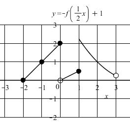
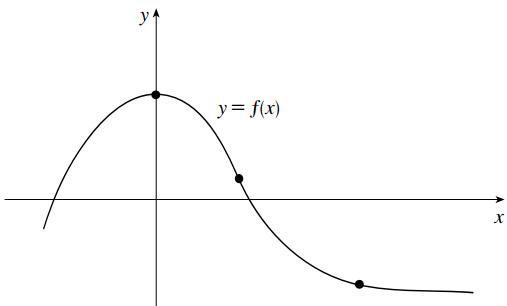
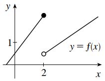
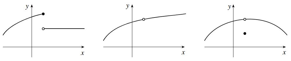
(a) The range of ( ) yfx = shown is {0,1,2,3}
(b) The range of the function ()yfx =− is{1,0,1,2,3}
(c) The range of the function (())yffx = is{1,0,1,2,}
1.3.9

1.3.10
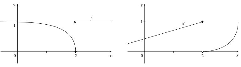
(a) The domain of ()ygx = is (0,)
(b) The domain of ( )()yfgx =+ is the domain of f which is ) 2,3.
(c) The domain of (())fgx is roughly 2,2.25.
(d) The domain of ( ) yfx = is the domain of f which is ) 2,3.
(e) The domain of (2)yfx = is 3 2 [1,).
1.3.11
(a) The domain of () f yx g =
is ) ( 1,11,3.−
(b) The domain of ( )( )ygfx = is ) ) 7,63,3.−−−
(c) The domain of ( ) yfx = is ) ( ) ( ) 8,66,66,8. −−−
(d) The domain of (2)yfx = is [4,3)(3,4). −
or
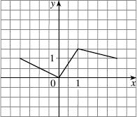
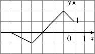
(a) (b)
Solution and Answer Guide: Stewart Kokoska, Calculus: Concepts and Contexts, 5e, 2024, 9780357632499, Chapter 1: Section 1.3
1.3.12
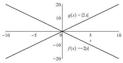
The graphs of ()2 fxx =− and ()2 gxx = are reflections through the x-axis.
1.3.13
First graph the function 1(), = gxx then shift to the left one unit ( ) 2()1. =+gxx Finally, shift up 2 units to plot ()12. =++fxx

1.3.14
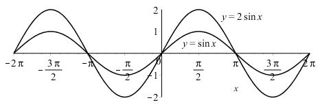
(a) The graph of 2sin yx = is the graph of sin yx = stretched vertically by a factor of 2.
(b) The graph of 1 yx =+ is the graph of yx = shifted up 1 unit.

1.3.15
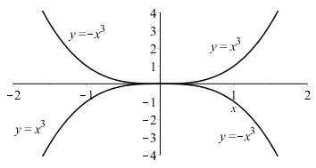
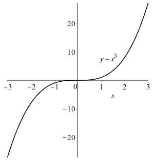
Start with the graph of 3 yx = and reflect about the x-axis.
or
1.3.16
Start with the graph of 2 yx = and shift 3 units to the right.

1.3.17
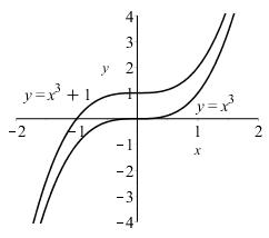
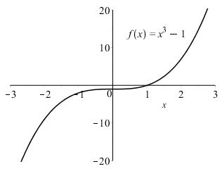
Start with the graph of 3 1 yx=+ and shift up 1 unit:
1.3.18
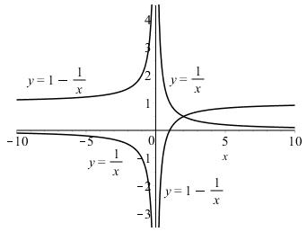
Start with the graph of 1 y x = reflect about the x-axis, and then shift up 1 unit.
1.3.19
Start with the graph of cos,yx = compress horizontally by a factor of 3, then stretch vertically by a factor of 2:

1.3.20
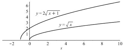
Start with the graph of ,yx = shift 1 unit to the left, and then stretch vertically by a factor of 2:
1.3.21
First note that 2245(2)1.yxxx =−+=−+ Now start with the graph of 2 , yx = shift 2 units to the right, then up 1 unit:
1.3.22
Start with the graph of sin,yx = compress horizontally by a factor of π, then shift up 1 unit.

1.3.23
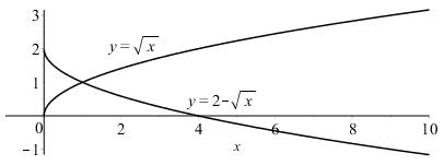
Start with the graph of ,yx = reflect about the xaxis, and then shift up 2 units:
1.3.24
Start with the graph of cos,yx = stretch vertically by a factor of 2, reflect about the x-axis, and then shift up 3 units:

1.3.25
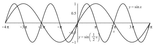
Start with the graph of sin yx = and stretch horizontally by a factor of 2:
1.3.26
Start with the graph of yx = and shift 2 units down:

1.3.27
Start with the graph of yx = and shift 2 units to the right:

1.3.28
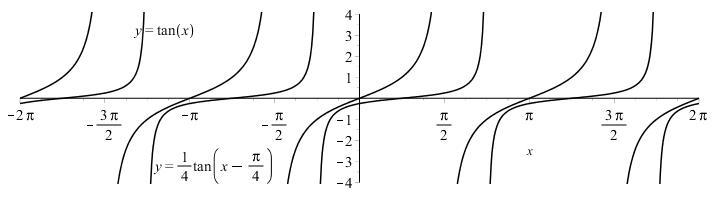
Start with the graph of tan,yx = shift π/4 units to the right, then compress vertically by a factor of 4.
1.3.29
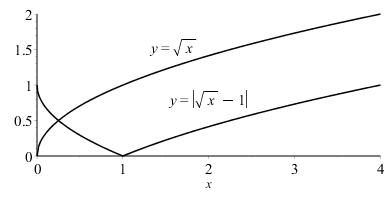
Start with the graph of yx = , shift down 1 unit, and then reflect the portion from 0 x = to 1 x = across the x –axis to obtain the graph of 1. yx=−
1.3.30
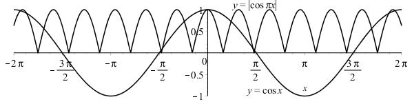
Start with the graph of cos,yx = shrink it horizontally by a factor of π, then reflect all the parts of the graph below the x-axis about the x-axis.
1.3.31
This is just like the solution to Example 4 except the amplitude of the curve (the 30N curve in Figure 9 on June 21) is 14122 −= . So the function is ( ) ( ) 2 122sin80 365 Ltt
. March 31 is the 90th day of the year, so the model gives ( ) 9012.34 h L . The daylight time (5:51 AM to 6:18PM) is 12 hours and 27 minutes, or 12.45 h . The model value differs from the actual value with a relative error of 12.4512.34 0.009 12.45 , less than 1%
1.3.32
Using a sine function to model the brightness of Delta Cephei as a function of time, we take its period to be 5.4 days, its amplitude to be 0.35 (on the scale of magnitude), and its average magnitude to be 4.0. If we let t = 0 at the time of average brightness, then the magnitude (brightness) as a function of time t in days can be modeled by ( ) 2 5.4 ()4.00.34sin. Mtt =+
1.3.33
The water depth D(t) can be modeled by a cosine function with amplitude (12 – 2)/2 = 5 m, average magnitude (12 + 2)/2 = 7 m, and period 12 hours. High tide occurred at 1:02 PM
Solution and Answer Guide: Stewart Kokoska, Calculus: Concepts and Contexts, 5e, 2024, 9780357632499, Chapter 1: Section 1.3
( ) 391 2 6030 h 13, h t = = so the curve begins a cycle at time 391 30 h t = (we need to shift 391 30 units to the right). Thus ( ) ( ) ( ) ( ) 391391 300 2 3 126 ()5cos75cos7, Dttt =−+=−+ where D is measured in meters and t is the number of hours after midnight.
1.3.34
The total volume of air V(t) in the lungs can be modeled by a sine function with amplitude (2500 – 200)/2 = 250 mL, average volume = (2500 + 2000)/2 = 2250 mL, and period 4 seconds. Thus 2 42 ()250sin2250250sin2250, Vttt =+=+ where V is in mL and t is in seconds.
1.3.35
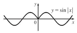
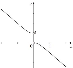
(a) To obtain ( ) yfx = , the portion of the graph of ( )yfx = to the right of the yaxis is reflected about the y -axis.
(b) sin yx =
(c) yx =

1.3.36
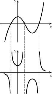
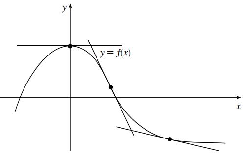
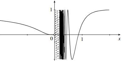
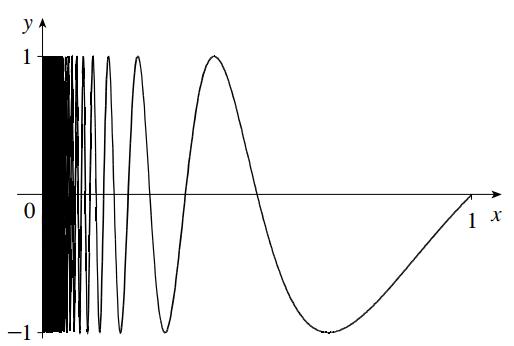
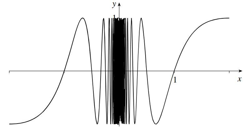
The most important features of the given graph are the x-incepts and the maximum and minimum points. The graph of 1/()yfx = has vertical asymptotes at the x-values where the x-intercepts are on the graph of ().yfx = The maximum of 1 on the graph of ()yfx =
or
Solution and Answer Guide: Stewart Kokoska, Calculus: Concepts and Contexts, 5e, 2024, 9780357632499, Chapter 1: Section 1.3
corresponds to a minimum of 1/1 = 1 on Similarly, the minimum on the graph of ()yfx = corresponds to a maximum on the graph of 1/().yfx = As the values of y get large (positively or negatively) on the graph of (),yfx = the values of y get close to zero on the graph of 1/().yfx =
1.3.37
(a) ( ) 32 ()51.fgxxx +=+− Its domain is all real numbers.
(b) ( ) 32 ()1.fgxxx −=−+ Its domain is all real numbers.
(c) ( ) 5432 ()362. fgxxxxx =+−− Its domain is all real numbers.
(d) ( ) 32 2 2 /(). 31 xx fgx x + = Its domain is 3 |. 3 xx
1.3.38
(a) ( ) 2 ()31.fgxxx +=−+− Its domain is ( ,11,3.−−
(b) ( ) 2 ()31.fgxxx −=−−− Its domain is ( ,11,3.−−
(c) ( ) 2 ()31.fgxxx=−− Its domain is ( ,11,3.−−
(d) ( ) 2 3 /(). 1 x fgx x = Its domain is ( ) ( ,11,3.−−
1.3.39
(a) ( ) 2 ()335.fgxxx=++ Its domain is all real numbers.
(b) ( ) ( )2 2 ()353593230.gfxxxxx =+++=++ Its domain is all real numbers.
(c) ( )()3(35)5920.ffxxx =++== Its domain is all real numbers.
or
Solution and Answer Guide: Stewart Kokoska, Calculus: Concepts and Contexts, 5e, 2024, 9780357632499, Chapter 1: Section 1.3
(d) ( ) ( )2 22432 ()22. ggxxxxxxxxx =+++=+++ Its domain is all real numbers.
1.3.40
(a) ( ) 332 ()(14)26448121. fgxxxxx =−−=−+−− Its domain is all real numbers.
(b) ( ) ( )4 3 ()12.gfxx=−− Its domain is all real numbers.
(c) ( ) 33963 ()(2)261210.ffxxxxx =−−=−+− Its domain is all real numbers.
(d) ( )()14(14)163.ggxxx =−−=− Its domain is all real numbers.
1.3.41
(a)( )()42.fgxx=− Its domain is 1 2 |.xx−
(b) ( )()413.gfxx=+− Its domain is |1.xx−
(c) ( )()11.ffxx=++ Its domain is |1.xx−
(d) ( ) ( ) ()44331615.ggxxx =−−=− Its domain is all real numbers.
1.3.42
(a) ( ) ( ) 2 ()sin1.fgxx=+ Its domain is all real numbers.
(b) ( ) 2 ()sin1.gfxx=+ Its domain is all real numbers.
(c) ( )()sin(sin) ffxx = . Its domain is all real numbers.
(d) ( ) ( )2 242 ()1122.ggxxxx=++=++ Its domain is all real numbers.
1.3.43
(a)( ) 2 12265 (). 21(1)(2) xxxx fgx xxxx ++++ =+= ++++ Its domain is |2,1.xx−−
(b) ( ) 2 2 1 11 (). 121 2 x xx x gfx xx x x ++ ++ == ++ ++ Its domain is |1,0.xx−
or
or
to a
Solution and Answer Guide: Stewart Kokoska, Calculus: Concepts and Contexts, 5e, 2024, 9780357632499, Chapter 1: Section 1.3
(c) ( ) 42 2 1131 (). 1 (1) xx ffxx xxx x x ++ =++= + + Its domain is |0.xx
(d) ( ) 1 2123 (). 135 2 2 x x x ggx x x x + + + + == + + + + Its domain is 5 3 |2,.xx−−
1.3.44
(a) ( ) sin2 (). 1sin2 x fgx x = + Its domain is ( ) 3 4 |,.xxnn +
(b) ( )()sin. 1 x gfx x = + Its domain is |1.xx−
+ + ===
(c) ( ) (1) 1 1 () 21 1 1(1) 1 1 x x x x x x ffx x x x x x x
+ ++ + + Its domain is 1 2 |1,.xx−−
(d) ( )()sin(2sin2). ggxx = Its domain is all real numbers.
1.3.45 ( ) ( ) ( ) ( ) 222 ()sin(3sin2fghxfgxfxx ===−
1.3.46 ( ) ( )2 ()44fghxxx=−=−
1.3.47 ( ) ( ) ( ) ( ) ( ) ( ) 22 33363 ()222341 fghxfgxfxxxx =+=+=+−=++
1.3.48 ( ) ( ) ( ) 33 3 33()tan 11 xx fghxfgxf xx
or duplicated, or
to a
If 42 (),()2, fxxgxxx ==+ then( ) ( )4 2 ()2(). fgxxxFx =+=
1.3.50
If 2 (),()cos. fxxgxx == then( ) ( )2 2 ()coscos(). fgxxxFx ===
1.3.51
If 3 (),(), 1 x fxgxx x == + then( ) 3 3 ()(). 1 x fgxFx x == +
1.3.52
If 3 (),(), 1 x fxxgx x == + then( ) 3 ()(). 1 x fgxFx x == +
1.3.53
If 2 ()sectan,(), ftttgtt == then( ) ( ) ( ) ( ) 222 ()sectan(). fgtftttFt ===
1.3.54
If (),()tan, 1 t ftgtt t == + then( ) ( ) tan ()tan(). 1tan t fgtftFt t === + 1.3.55
Let (),()1,(). fxxgxxhxx ==−= Then
( ) ( ) ( ) ( ) ()11(). fghxfgxfxxFx ==−=−= 1.3.56
Let 8 (),()2,(). fxxgxxhxx ==+= Then
( ) ( ) ( ) ( ) 8 ()22(). fghxfgxfxxFx ==+=+=
1.3.57
Let 2 (),()sin,()cos. fttgtthtt === Then
( ) ( ) ( ) ( ) 22 ()cossin(cos)(sin(cos))sin(cos)(). fghtfgtftttFt =====
1.3.58
Solution and Answer Guide: Stewart Kokoska, Calculus: Concepts and Contexts, 5e, 2024, 9780357632499, Chapter 1: Section 1.3
Let 3 1 ()tan,(),(). fttgthtt t === Then
( ) ( ) ( ) 3 33 11 ()tan(). fghtfgtfFt tt
1.3.59
(a) ((1))(6)5fgf== (b) ((1))(3)2gfg==
(c) ((1))(3)4fff== (d) ((1))(6)3ggg==
(e) ( )(3)((3))(4)1gfgfg=== (f) ( )(6)((6))(3)4fgfgf===
1.3.60
(a) ((2))(5)4fgf== (b) ((0))(0)3gfg== (c)( )(0)((0))(3)0fgfgf=== (d) ( )(6)((6))(6)undefinedgfgfg===
(e) ( )(2)((2))(1)4ggggg−=−== (f) ( )(4)((4))(2)2fffff===−
1.3.61
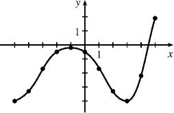
1. To find a particular value of (()),fgx say for x = 0, we note from the graph that g(0) ≈ 2.8 and f(2.8) ≈ –0.5. Thus ((0))(2.8)0.5.fgf− The other values listed in the table are obtained in a similar fashion.
Solution and Answer Guide: Stewart Kokoska, Calculus: Concepts and Contexts, 5e, 2024, 9780357632499, Chapter 1: Section 1.3
1.3.62
(a) Using the relationship distance = rate time with the radius as the distance, we have 60.rt =
(b) ( ) ( )2 22 ()(())603600. ArArtArttt ==== The area of the circle is increasing at a rate of 3600π cm/s2 .
1.3.63
(a) The radius of the balloon is increasing at a rate of 2 cm/s, so ( ) ()2in cm rtt =
(b) Using 3 4 3 , Vr = we get( ) ( )3 3 32 4 33 ()(())(2)2. VrtVrtVttt ==== This tells us the volume of the balloon (in cm3) as a function of time in seconds.
1.3.64
From the figure, we have a right triangle with legs of length 6 and d, and hypotenuse s. By the Pythagorean Theorem, 22226()36.dssfdd +===+

(b) Using d = rt, we find d = (30 km)×(t hours) = 30t (in km). Thus ()30. dgtt ==
(c) ( ) 2 ()(())(30)90036.fgtfgtftt ===+ This represents the distance between the ship and the lighthouse as a function of the time elapsed since noon.
Solution and Answer Guide: Stewart Kokoska, Calculus: Concepts and Contexts, 5e, 2024, 9780357632499, Chapter 1: Section 1.3
1.3.65
(a) ()350. drtdtt ==
(b) There is a Pythagorean relationship involving the legs with length d and 1 and the hypotenuse with length s: 2221.ds += Thus, 2 ()1.sdd=+
(c) ( ) ( ) 2 ()(())(350)350)1sdtsdtstt===+
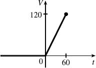
1.3.66
(a) Heaviside function:

(b)
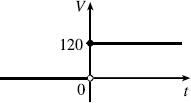
(c) Starting with the equation in part (b), we replace 120 with 240 to reflect the different voltage. Also, because we are starting 5 units to the right of t = 0, we replace t with t – 5. Thus the formula is ()240(5).VtHt=−
1.3.67
(a) ( ) ( )RttHt =

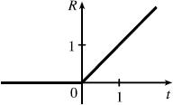
(b)
so ( ) ( ) 2,60VttHtt= .
Solution and Answer Guide: Stewart Kokoska, Calculus: Concepts and Contexts, 5e, 2024, 9780357632499, Chapter 1: Section 1.3
(c) ( ) ( ) 0 if 7 47 if732 t Vt tt =
so ( ) ( ) ( ) 477,32VttHtt =−− .

1.3.68
If ( ) 11 fxmxb =+ and ( ) 22 gxmxb =+ , then
( )( ) ( ) ( ) ( ) ( ) 22122112121. fgxfgxfmxbmmxbbmmxmbb ==+=++=++
So fg is a linear function with slope 12mm .
1.3.69
If 2 ()1.04, Axx = then( ) 2()1.04 AAxx = , and( ) 3()1.04 AAAxx = , and ( ) 4 ()1.04. AAAAxx = These compositions represent the investment amounts after 2, 3 and 4 years respectively. After n compositions, the investment amount would be 1.04. n x
1.3.70
(a) If ()21gxx=+ and 2 ()6fxx=+ then ( ) 22 21(21)6447 fgfxxxx =+=++=++ ().hx =
(b) If ()4fxx=+ and 2 ()1gxxx=+− then
Solution and Answer Guide: Stewart Kokoska, Calculus: Concepts and Contexts, 5e, 2024, 9780357632499, Chapter 1: Section 1.3
( ) 2213(1)5fgfxxxx=+−=+−+ 22 3335332(). xxxxhx =+−+=++=
1.3.71
If ()4fxx=+ and ()41hxx=− then hgf = if ()417gxx=− .
1.3.72
Suppose g is an even function and .hfg = Then ( ) ()()(()) hxfgxfgx −=−=−
(()() fgxhx== so hfg = is an even function.
1.3.73
Suppose g is an odd function and hfg = First suppose f is an odd function.
Then ( ) ()() hxfgx −=− (())(())(())() fgxfgxfgxhx =−=−=−=− so hfg = is an odd function.
Now assume f is an even function. Then ( ) ()() hxfgx −=−
(())(())(())() fgxfgxfgxhx =−=−== so hfg = is an even function.
If f is neither either nor odd, hfg = will be neither even nor odd.
1.3.74
(a) We need to examine ( ). hx
( ) ( )( ) ( ) ( ) ( ) ( ) ( ) ( ) ( ) sinsinsin[becauseis even] hxfgxfxfxfxffgxhx −=−=−=−===
Because ( ) ( ), hxhx −= h is an even function.
(b) We need to examine ( ). hx
( ) ( )( ) ( ) ( ) ( ) ( )
( ) ( ) ( ) ( ) ( ) coscos [because isodd] cos hxgfxfxfxf fxgfxhx −=−=−=− ===
Because ( ) ( ), hxhx −= h is an even function.
(c) We need to examine ( ). kx
( ) ( )( ) ( ) ( ) ( ) ( ) ( ) ( ) ( ) [sinceis even] kxfghxfghxfghxhkx −=−=−==
or
to a
Solution and Answer Guide: Stewart Kokoska, Calculus: Concepts and Contexts, 5e, 2024, 9780357632499, Chapter 1: Section 1.3
Because ( ) ( ), kxkx −= k is an even function. Note that the result does not depend on whether the functions f and g are each even, odd, or neither.
Solution and Answer Guide
STEWART KOKOSKA, CALCULUS: CONCEPTS AND CONTEXTS, 5E, 2024, 9780357632499, CHAPTER 1: SECTION 1.1
TABLE OF CONTENTS
End of Section Exercise Solutions......................................................................................1
END OF SECTION EXERCISE SOLUTIONS
1.1.1
(a) (1)3 f =
(b) (1)0.2 f −−
(c) ()1fx = when x = 0 and x = 3.
(d) ()0fx = when x ≈ –0.8.
(e) The domain of f is 24. x − The range of f is 13. y −
(f) f is increasing on the interval 21. x −
1.1.2
(a) (4)2;(3)4 fg−=−=
(b) ()() fxgx = when x = –2 and x = 2.
(c) ()1fx =− when x ≈ –3.4.
(d) f is decreasing on the interval 04. x
(e) The domain of f is 44. x − The range of f is 23. y −
(f) The domain of g is 44. x − The range of g is 0.54. y
1.1.3
(a) (2)12 f = (b) (2)16 f = (c) 2 ()32 faaa=−+
Solution and Answer Guide: Stewart Kokoska, Calculus: Concepts and Contexts, 5e, 2024, 9780357632499, Chapter 1: Section 1.1
(d) 2 ()32 faaa−=++ (e) 2 (1)354 faaa+=++ (f) 2 2()624 fxaa=−+
(g) 2 (2)1222 faaa=−+ (h) 242 ()32 faaa=−+
(i) ( )2 2 2432 ()32961344 faaaaaaa =−+=−+−+ (j) ( ) ( ) 2 22 ()323362 fahahahahahah +=+−++=++−−+
1.1.4 222(3)(3)(43(3)(3))49396)3 (3) fhfhhhhhhh h hhhh +−++−+−+−−−−− ====−+
1.1.5 ()() fahfa h +− = ( ) 22 32233 22 33 33 33 haahh aahahha aahh hh ++ +++− ==++ 1.1.6 ()() fxfa xa = 11 1 () ax ax xaaxax xaxaaxxaax ===− 1.1.7 ()(1) 1 fxf x = 313332211211111111 111111 xxxxxx xxxxx xxxxxx ++++−−−+− ++++++
1.1.8 The domain of 2 4 ()9 x fx x + = is |3,3.xx− 1.1.9 The domain of 3 2 25 () 6 x fx xx = +− is |3,2.xx−
Solution and Answer Guide: Stewart Kokoska, Calculus: Concepts and Contexts, 5e, 2024, 9780357632499, Chapter 1: Section 1.1
1.1.10
The domain of 3 ()21ftt=− is all real numbers.
1.1.11 ( ) 32 gttt =−−− is defined when 03 3 t t and 2 02 t t Thus, the domain is 2, t or ( 2 . ,−
1.1.12
The domain of 2 4 1 () 5 hx xx =− is( ) ( ) ,05,.−
1.1.13
The domain of ()2 Fpp =− is 04. p
1.1.14
The domain of 1 () 1 1 1 u fu u + = + + is |2,1.uu−−
1.1.15
(a) This function shifts the graph of y = |x| down two units and to the left one unit.
(b) This function shifts the graph of y = |x| down two units
(c) This function reflects the graph of y = |x| about the x-axis, shifts it up 3 units and then to the left 2 units.
(d) This function reflects the graph of y = |x| about the x-axis and then shifts it up 4 units.
(e) This function reflects the graph of y = |x| about the x-axis, shifts it up 2 units then four units to the left.
(f) This function is a parabola that opens up with vertex at (0, 5). It is not a transformation of y = |x|.
1.1.16
(a) ( ) ( ) ( ) ( ) 221101gfxgxx=+=+
(b) ( ) ( ) ( ) ( ) 2 41044011601fgf==+=
(c) ( ) ( ) ( ) ( ) ( ) 11011010100ggg−=−=−=−
or
or
to a
Solution and Answer Guide: Stewart Kokoska, Calculus: Concepts and Contexts, 5e, 2024, 9780357632499, Chapter 1: Section 1.1
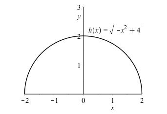
1.1.17
The domain of 2 ()4 hxx =− is 22, x − and the range is 02. y The graph is the top half of a circle of radius 2 with center at the origin.
1.1.18
The domain of ()1.62.4fxx=− is all real numbers.

1.1.19
The domain of 2 1 () 1 t gt t = + is |1.tt−
1.1.20
The domain of 2 1 ()1 x fx x = is |1,1.xx−

Solution and Answer Guide: Stewart Kokoska, Calculus: Concepts and Contexts, 5e, 2024, 9780357632499, Chapter 1: Section 1.1
1.1.21
The domain of 3 ()1fxx=− is all real numbers.
1.1.22
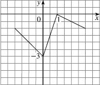
1.1.24 ( ) 3321 f −=−+=− ( ) 0101 f =−= ( ) 2121 f =−=− 1.1.25

Solution and Answer Guide: Stewart Kokoska, Calculus: Concepts and Contexts, 5e, 2024, 9780357632499, Chapter 1: Section 1.1
( ) ( ) 9 1 22333 f −=−−=
( ) ( ) 1 2 0303 f =−=
( ) ( ) 22251 f =−=−
1.1.26
( ) 3312 f −=−+=−
( ) 2 000 f ==
( ) 2 224 f == 1.1.27
( ) 31 f −=−
( ) 01 f =−
( ) ( ) 27223 f =−=

1.1.28

Recall that the slope m of a line between the two points ( ) 11 , xy and ( ) 22 , xy is 21 21 yy m xx = and an equation of the line connecting those two points is ( )11 yymxx −=− . The slope of the line segment joining the points ( )1,3 and ( )5,7 is
or
or
Solution and Answer Guide: Stewart Kokoska, Calculus: Concepts and Contexts, 5e, 2024, 9780357632499, Chapter 1: Section 1.1
( )73 5 512 = , so an equation is ( ) ( ) 5 31. 2 yx−−=− The function is ( ) 511 ,15 22 fxxx=−
1.1.29
The slope of the line segment joining the points ( )5,10 and ( )7,10 is ( ) 10105 753 =− , so an equation is ( ) 5 105. 3 yx−=−−− The function is ( ) 55 ,57 33 fxxx =−+−
1.1.30
We need to solve the given equation for 22 . (1)0(1)1 yxyyxyx +−=−=−−=− 1 yx =− . The expression with the positive radical represents the top half of the parabola, and the one with the negative radical represents the bottom half. Hence, we want ( ) 1 fxx =−− . Note that the domain is 0 x .
1.1.31
222222 (2)4(2)4 24 24 xyyxyxyx +−=−=−−=−=− . The top half is given by the function ( ) 2 24,22fxxx =+−−
1.1.32
For 03 x , the graph is the line with slope 1 and y -intercept 3 , that is, 3 yx=−+ . For 35 x , the graph is the line with slope 2 passing through ( )3,0 ; that is, ( )023yx−=− , or 26yx=− . So the function is ( ) 3 if03 26 if35 xx fx xx
1.1.33
For 42 x −− , the graph is the line with slope 3 2 passing through ( )2,0 ; that is, ( ) 3 02 2 yx−=−−− , or 3 3 2 yx=−− . For 22 x − , the graph is the top half of the circle with center ( )0,0 and radius 2 . An equation of the circle is 22 4 xy+= , so an
or
equation of the top half is 2 4 yx =− . For 24 x , the graph is the line with slope
1.1.34
From Figure 1.1 in the text, the lowest point before the end of the Super Bowl occurs at about ( ) ( ) ,145,300,tr = where t is measured in minutes. The highest point occurs at about ( ) 20,360. Thus, the range of the rate of water usage is 30 60 0 3 t Written in interval notation, we get 300,360.
1.1.35
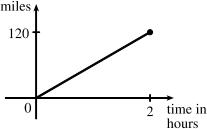
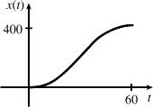
Example 1: A car is driven at 60 mph for 2 hours. The distance d traveled by the car is a function of the time t. The domain of the function is {|02}, tt where t is measured in hours. The range of the function is {|0120}, dd where d is measured in miles.
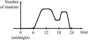
Example 2: At a certain university, the number of students N on campus at any time on a particular day is a function of the time t after midnight. The domain of the function is {|024}, tt where t is measured in hours. The range of the function is {|0}, NNk where N is an integer and k is the largest number of students on campus at one time.
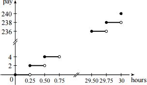
Example 3: A certain employee is paid $8.00 per hour and works a maximum of 30 hours per week. The number of hours worked is rounded down to the nearest quarter hour. This employee’s gross weekly pay P is a function of the number of hours worked h. The domain of the function is [0, 30], and the range of the function is {0, 2.00, 4.00, . . . , 238.00, 240.00}.
1.1.36
This is not the graph of a function because it does not pass the vertical line test.
1.1.37
This is the graph of a function. The domain is 22 x − and the range is 13. y −
1.1.38
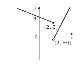
This is the graph of a function. The domain is 32 x − and the range is
32 y −−
1.1.39
13. y −
This is not the graph of a function because it does not pass the vertical line test.
1.1.40
(a) When t = 1950, T ≈ 13.8℃, so the global average temperature in 1950 was about 13.8℃.
(b) When T = 14.2℃, t ≈ 1990.
(c) The average global temperature was smallest in 1910 (the year corresponding to the lowest point on the graph) and the largest in year 2016 (the year corresponding to the highest point on the graph).
(d) When t = 1910, T ≈ 13.5℃, and when t = 2016, T ≈ 14.9℃. Thus, the range of T is about [13.5, 14.9].
1.1.41
(a) The width varies from near 0 mm to about 1.6 mm, so the range of the ring width function is approximately [0, 1.6].
(b) According to the graph, the earth gradually cooled from 1550 to 1700, warmed into the late 1700s, cooled again into the late 1800s, and has been steadily warming since then. In the mid-19th century, there was variation that could have been associated with volcanic eruptions.
1.1.42
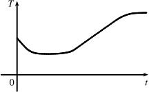
The water will cool down almost to freezing as the ice melts. Then, when the ice has melted, the water will slowly warm up to room temperature.
1.1.43
The graph indicates that runner A won the race, reaching the finish line at 100 meters in about 15 seconds, followed by runner B with a time of about 19 seconds, and then by runner C who finished in around 23 seconds. Runner B initially led the race, followed by C, and then A. Runner C passed runner B to lead for a while. Then runner A passed first runner B, then passed runner C to take the lead and finish first. All three runners finished the race.
1.1.44
(a) The power consumption at 6AM is 500MW , which is obtained by reading the value of power P when 6 t = from the graph. At 6 PM we read the value of P when 18 t = , obtaining approximately 730MW .
(b) The time of lowest power consumption is determined by finding the time for the lowest point on the graph, 4, t = or 4 AM. The time of highest power consumption corresponds to the highest point on the graph, which occurs just before 12, t = or right before noon. These times are reasonable, considering the power-consumption schedules of most individuals and businesses.
1.1.45
The summer solstice (longest day of the year) is around June 21, and the winter solstice (shortest day) is around December 22 (in the northern hemisphere). Therefore a reasonable graph for the number of hours of daylight vs. time of year is here:

1.1.46
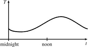
The graph will depend upon geographical location, but here is one graph of the outdoor temperature vs. time on a spring day:
1.1.47
Solution and Answer Guide: Stewart Kokoska, Calculus: Concepts and Contexts, 5e, 2024, 9780357632499, Chapter 1: Section 1.1
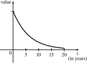
The value of the car will decrease rapidly initially, then somewhat less rapidly.
1.1.48
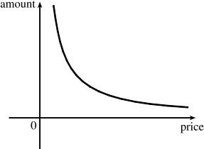
As the price increases, the amount of coffee sold will decrease:
1.1.49
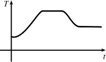
The temperature of the pie would increase rapidly, level-off to oven temperature, decrease rapidly when removed from the oven, and then level-off to room temperature:
1.1.50
Here is a rough graph of the height of the grass on a lawn that is mown every Wednesday:

Solution and Answer Guide: Stewart Kokoska, Calculus: Concepts and Contexts, 5e, 2024, 9780357632499, Chapter 1: Section 1.1

(b)
(c) (d)
Solution and Answer Guide: Stewart Kokoska, Calculus: Concepts and Contexts, 5e, 2024, 9780357632499, Chapter 1: Section 1.1
1.1.52
(a)
(b) The temperature at 9 AM appears to have been roughly 51oF.
1.1.53 (a)
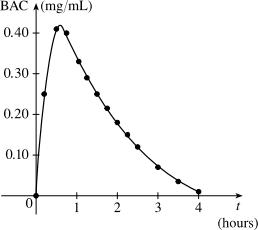
(b) The rate or BAC jumps rapidly from zero to the maximum of 0.41 mg/mL. The concentration then gradually decreases over the next four hours to near zero. 1.1.54
With radius r + 1, the balloon has volume 44332 33 (1)(1)(331). Vrrrrr +=+=+++ We wish to find the amount of air required to inflate the balloon from a radius of r to r+1 inches. Hence we need to find the difference 44323 33(1)()(3331) VrVrrrrr +−=++++− 2 4 3 (331). rr =++
1.1.55
Let the length and width of the rectangle be l and w. Then the perimeter is 2220 lw+= and the area is .Alw = Solving the first equation for win terms of l gives 202 10. 2 l wl ==− Thus 2 ()(10)10. Alllll =−=− Since the length must be positive, the
Solution and Answer Guide: Stewart Kokoska, Calculus: Concepts and Contexts, 5e, 2024, 9780357632499, Chapter 1: Section 1.1
domain of A is 0 < l < 10. If we further restrict l to be larger than w, the 5 < l < 10 would be the domain.
1.1.56
Let the length and width of the rectangle be l and w. Then the area is lw = 16 so that w = 16/l. The perimenter is 22, Plw =+ so ( ) ()2216/232/, Plllll =+=+ and the domain of P is l > 0 since the lengths must be positive. If we further require l to be larger than w, then the domain would be l > 4.
1.1.57
Let the length of a side of the triangle be x. Then by the Pythagorean Theorem, the height y of the triangle satistfies ( )2 2 1 2 , yx = so that 2222 3 1 44 yxxx =−= and 3 2 .yx =
Using the formula for the area A of a triangle, A = ½(base)(height), we find ( ) 2 33 1 224 (), Axxxx == with domain x > 0.
1.1.58
Let the length, width, and height of the closed rectangular box be denoted by l, w, and h respectively. The length is twice the width, so l = 2w. The volume V of the box is V = lwh. Since V = 8, we have 2 22 84 8(2)82, 2 wwhwhh ww ==== so 2 4 ().hfw w ==
1.1.59
Let each side of the base of the box have length x, and let the height of the box be h. Since the volume is 2, we know that 2 = hx2 so that h = 2/x2, and the surface area is 2 4.Sxxh =+ Thus, ( ) 222 ()42/8/, Sxxxxxx =+=+ with domain x > 0.
1.1.60
The area of the window is ( ) 2 2 11 22 8, x Axhxxh =+=+ where h is the height of the rectangular portion of the window. The perimeter is 1 2 230Phxx =++= 1 2 230hxx =−− ( ) 1 2 602.hxx
Thus, 2 602 () 48 xxx Axx
Since the lengths x and h must be positive, we have x > 0 and h > 0. For h > 0, we have
or
Solution and Answer Guide: Stewart Kokoska, Calculus: Concepts and Contexts, 5e, 2024, 9780357632499, Chapter 1: Section 1.1
Therefore the domain of A is 60 0. 2 x + 1.1.61
The height of the box is x and the length and width are 202,122. lxwx =−=− Then V = lwx so 232 ()(202)(122)4(10)(6)4(6016)464240. Vxxxxxxxxxxxxx =−−=−−=−+=−+
Because the sides must have positive lengths, 0202010;lxx − 06;wx and x > 0. Combining these restrictions indicates the domain is 0 < x < 6.
1.1.62
We can model the monthly cost with a piecewise function: 35if 02 (). 355(2)if2 x Cx xx
= +−

1.1.63
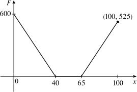
We can model the amount of the fine with a piecewise function: 15(40),if040 ()0,if4065. 15(65),if65100 xx Fxx xx
1.1.64
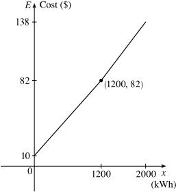
$100.06,if01200 () $100.06(1200)0.07(1200),if 400 xx Ex xx + =
1.1.65
(a) Here is the graph:
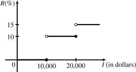
(b) On $14,000 tax is assessed on $4000, and 10% of $4000 is $400. On $26,000, tax is assessed on $16,000 and 10%($10,000) + 15%($6000) = $1000 + $900 = $1900.
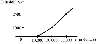
(c) As in part (b), there is $1000 tax assessed on $20,000 of income, so the graph of T is a line segment from (10,000, 0) to (20,000, 1000). The tax on $30,000 is $2500, so the graph of T for x > 20,000 is the ray with the initial point (20,000, 1000) that passes through (30,000, 2500).
1.1.66
One example is the amount paid for cable or appliance repair in the home, usually measured to the nearest quarter hour. Another example is the amount paid by a student in college tuition fees, if the fees vary according to the number of credits for which the student registers.
1.1.67
The function f is odd because its graph is symmetric about the point (0, 0). The function g is even because its graph is symmetric across the y-axis.
1.1.68
Solution and Answer Guide: Stewart Kokoska, Calculus: Concepts and Contexts, 5e, 2024, 9780357632499, Chapter 1: Section 1.1
The function f is even because its graph is symmetric across the y-axis. The function g is neither even nor odd because it is not symmetric about the y-axis or the origin.
1.1.69
(a) If the point (5, 3) is on the graph of an even function then (–5, 3) must also be on the graph.
(b) If the point (5, 3) is on the graph of an odd function then (–5, –3) must also be on the graph.
1.1.70
(a) Here is the complete graph if f is even:
(b) Here is the complete graph if f is odd:
1.1.71

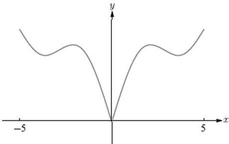
2 4 ()() 1 x fxfx x ==− + is an even function.
Solution and Answer Guide: Stewart Kokoska, Calculus: Concepts and Contexts, 5e, 2024, 9780357632499, Chapter 1: Section 1.1
1.1.73
()1 x fx x = + is neither even nor odd.
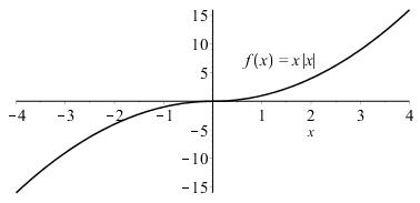
1.1.74
() fxxx = is an odd function because ()(). fxxxfx −=−−=−
1.1.75
2424 ()1313()()() fxxxxxfx =+−=+−−−=− is an even function.
1.1.76
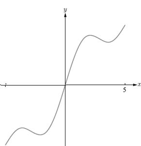
35 ()13 fxxx =+− is neither even nor odd.


Solution and Answer Guide: Stewart Kokoska, Calculus: Concepts and Contexts, 5e, 2024, 9780357632499, Chapter 1: Section 1.1
1.1.77
(i) If f and g are both even functions, then ( ) ( )fxfx −= and ( ) ( )gxgx −= . Now
( )( ) ( ) ( ) ( ) ( ) ( )( ), so fgxfxgxfxgxfgxfg +−=−+−=+=++ is an even function.
(ii) If f and g are both odd functions, then ( ) ( )fxfx −=− and ( ) ( )gxgx −=− . Now
( )( ) ( ) ( ) ( ) ( ) ( ) ( ) ( )( ),so fgxfxgxfxgxfxgxfgxfg +−=−+−=−+−=−+=−++
is an odd function.
(iii) If f is an even function and g is an odd function, then
+−=−+−=+−=−
( )( ) ( ) ( ) ( ) ( ) ( ) ( )fgxfxgxfxgxfxgx
, which is not ( )( )fgx + nor
( )( )fgx−+ , so fg + is neither even nor odd. (Exception: if f is the zero function, then fg + will be odd. If g is the zero function, then fg + will be even.)
1.1.78
(i) If f and g are both even functions, then ( ) ( )fxfx −= and ( ) ( )gxgx −= . Now ( )( ) ( ) ( ) ( ) ( ) ( )( ), so fgxfxgxfxgxfgxfg −=−−== is an even function
(ii) If f and g are both odd functions, then ( ) ( )fxfx −=− and ( ) ( )gxgx −=− . Now
( )( ) ( ) ( ) ( ) ( ) ( ) ( ) ( )( ),so fgxfxgxfxgxfxgxfgxfg
is an even function.
(iii) If f is an even function and g is an odd function, then ( )( ) ( ) ( ) ( ) ( ) ( ) ( ) ( )( ),so fgxfxgxfxgxfxgxfgxfg
is an odd function.
Solution and Answer Guide
TABLE OF CONTENTS
End of Section Exercise
END OF SECTION EXERCISE SOLUTIONS
1.2.1
(a) ( ) 2log fxx = is a logarithmic function.
(b) ( ) 3 2 2 1 x gx x = is a rational function because it is a ratio of polynomials.
(c) ( ) 2 123 uttt =−+ is a polynomial of degree 2 (also called a quadratic function).
(d) ( ) 2 11.12.54 uttt =−+ is a polynomial of degree 2.
(e) ( ) 2/7 hxx = is a power function.
(f) ( ) ( ) ( ) 4232kxxx=−+ is a polynomial of degree 6.
(g) ( ) 5t vt = is an exponential function.
(h) ( ) 2sincos wttt = is a trigonometric function.
1.2.2
(a) 4 yx = is a power function and a polynomial of degree 4.
(b) ( ) 2325 22 yxxxx =−=− is a polynomial of degree 5.
(c) 1 x y x = + is a rational function because it is a ratio of polynomials.
Solution and Answer Guide: Stewart Kokoska, Calculus: Concepts and Contexts, 5e, 2024, 9780357632499, Chapter 1: Section 1.2
(d) 3 3 1 1 x y x = + is an algebraic function because it involves polynomials and roots of polynomials.
(e) 3/5 7 yx=+ is an algebraic function.
(f) 2 2 1 x y x = + is an algebraic function.
(g) 2 3 75 1 xx y xx −+ = +− is a rational function.
(h) tancos ytt =− is a trigonometric function.
1.2.3
(a) 2 yx = is the blue curve (function h) because it is a parabola.
(b) 5 yx = is the red curve (function f ) because it is an odd power function.
(c) 8 yx = is the green curve (function g) because it is an even power function whose degree is more than 2.
1.2.4
(a) 3 yx = is the blue curve (function f ) because it is a linear function.
(b) 3 yx = is the red curve (function g) because it is an odd power function.
(c) 3 yx = is the green curve (function h) because it is the cube-root function.
1.2.5
The domain and range of ()23fxx=− are all real numbers.
1.2.6
The domain of 2 ()4fxx=+ is all real numbers. The range is |4.yy
1.2.7
The domain of 3 ()1gxx=+ is all real numbers. The range is also all real numbers.
1.2.8
or
Solution and Answer Guide: Stewart Kokoska, Calculus: Concepts and Contexts, 5e, 2024, 9780357632499, Chapter 1: Section 1.2
The domain of 2 2 ()4 x gx x = is |2,2.xx− The range is |0.yy
1.2.9
The domain of 3 ()22 hxxx=++ is all real numbers. The range is also all real numbers.
1.2.10
The domain of ()2hxx=+ is |0.xx The range is |2.yy
1.2.11
The domain of 2 ()4fxx=+ is all real numbers. The range is |2.yy
1.2.12
The domain of 1 () 2 fx x = + is |2.xx− The range is |0.yy
1.2.13
The graph of ()4 x fx x = + has a vertical asymptote at 4 x =− and a horizontal asymptote at 1. y =
1.2.14
The graph of 2 () 3 x fx x = + has a vertical asymptote at 3 x =− and no horizontal asymptotes.
1.2.15
The graph of 2 () (2)(2) x gx xx = +− has a vertical asymptote at x = –2 and a horizontal asymptote at 0. y = 1.2.16
The graph of 3 ()1 x gx x = has a vertical asymptote at x = 1 and a horizontal asymptote at 0. y = 1.2.17
or
Solution and Answer Guide: Stewart Kokoska, Calculus: Concepts and Contexts, 5e, 2024, 9780357632499, Chapter 1: Section 1.2
The graph of 2 () 2 x hx x + = has a vertical asymptote at x = 2 and a horizontal asymptote at 0. y = 1.2.18
The graph of 3 1 ()1 x hx x + = has a vertical asymptote at 1 x = and a horizontal asymptote at 0. y = 1.2.19
By the Vertical Line Test, the given graph is the graph of y as a function of x 1.2.20
By the Vertical Line Test, the given graph is the graph of y as a function of x. 1.2.21
By the Vertical Line Test, the given graph is not the graph of y as a function of x. 1.2.22
By the Vertical Line Text, the given graph is not the graph of y as a function of x 1.2.23
The linear function such that (3)11 f = and (7)9 f = must have slope = 1911 2. 73 = An equation for this line is 2(3)1125.yxx =−+=+ 1.2.24 If ()35fxx=+ then ()() fbfa ba (35)(35)33 33. bababa bababa +−+−− ==== This will always be the value because the rate of change (i.e. “slope”) of a linear function is constant.
1.2.25
If ()52fxx=+ then ( )5()252 ()()552525 5. xhx fxhfxxhxh hhhh ++−+ +−++−− ====
1.2.26
The domain of 2 ()2(3)5fxx=−+ is all real numbers. The range is |5.yy 1.2.27
or
Solution and Answer Guide: Stewart Kokoska, Calculus: Concepts and Contexts, 5e, 2024, 9780357632499, Chapter 1: Section 1.2
A quadratic function with range{|6} yy such that (4)(4) fdfd +=− is 2()6(4)fxx=−− or 2 ()810. fxxx=−+− This function has a maximum of 6 that occurs when x = 4 and for all d, 2 (4)(4)6. fdfdd +=−=−
1.2.28
A root function for which g(64) = 4 is 3 (). gxx =
1.2.29
A rational function with a linear denominator which has an x-intercept at 4 and a vertical asymptote at x = 3 is 4 (). 3 x fx x =
1.2.30
A rational function that is undefined at x = 2 but does not have a vertical asymptote at 2 x = is 2 4 (). 2 x fx x =
1.2.31
(a) An equation for the family of linear functions with slope 2 is 2. yxb =+ Below is a graph of several members of this family.

(b) An equation for the family of linear functions such that (2)1 f = is 1 2 . b yxb =+ Below is a graph of several members of this family.
or
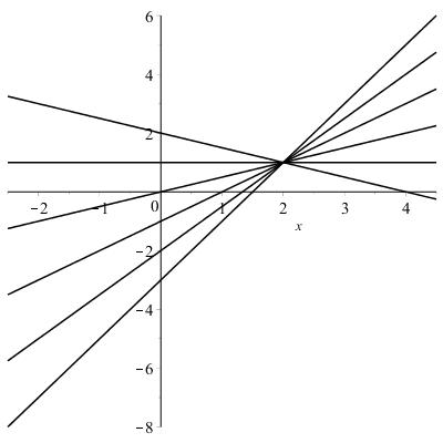
(c) The function 23yx=− belongs to both families in (a) and (b).
1.2.32
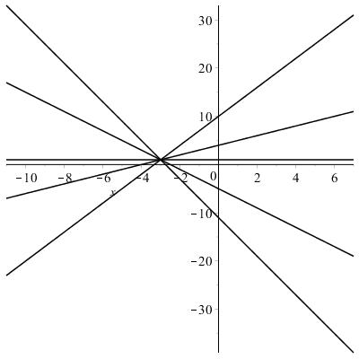
All members of the family of linear functions ()1(3) fxmx=++ go through the point (3,1). Below is a graph of several members of this family.
1.2.33
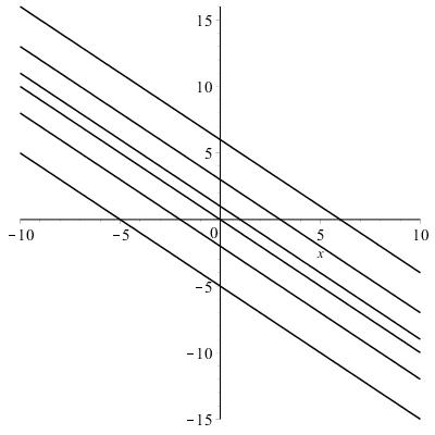
All members of the family of linear functions (). fxcx =− have a common slope of –1. Each has a y-intercept of (0, c). Below is a graph of several members of this family.
1.2.34
(a) The vertex of the parabola is ( )3,0 , so an equation is 2 (3)0yax=−+ . Since the point ( )4,2 is on the parabola, we'll substitute 4 for x and 2 for y to find 2 .2(43)2aaa=−= , so an equation is ( ) 22(3)fxx=− .
(b) The y -intercept of the parabola is ( )0,1 , so an equation is 2 1 yaxbx=++ . Since the points ( )2,2 and ( )1,2.5 are on the parabola, we'll substitute 2 for x and 2 for y as well as 1 for x and 2.5 for y to obtain two equations with the unknowns a and b ( ) ( ) 2,2:2421421 1,2.5:2.51 3.5 abab abab
( ) ( )221 + gives us 661 aa=−=− . From (2), 13.52.5 bb −+=−=− , so an equation is ( ) 2 2.51gxxx=−−+ .
1.2.35
. One expression for a cubic function f such that (1)6 f = , and (1)(0)(2)0 fff−=== is ()3(2)(1). fxxxx=−−+
1.2.36
One cubic function that is increasing on the interval (–∞, ∞) is 3 ():fxx =
Solution and Answer Guide: Stewart Kokoska, Calculus: Concepts and Contexts, 5e, 2024, 9780357632499, Chapter 1: Section 1.2
1.2.37
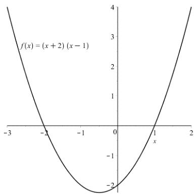
One quadratic function that intersects the x-axis at –2 is ()(2)(1) fxxx=+− :
1.2.38
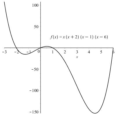
One fourth degree polynomial that has zeros –2, 0, 1 and 6 is ()(2)(1)(6). fxxxxx =+−−
1.2.39
Solution and Answer Guide: Stewart Kokoska, Calculus: Concepts and Contexts, 5e, 2024, 9780357632499, Chapter 1: Section 1.2
(a) In the equation 0.028.50,Tt=+ the slope of 0.02 indicates that for each additional year after 1900 the temperature is predicted to rise 0.02 ℃. This is the rate of change in temperature with respect to time. The T-intercept of 8.5 ℃ represents the average temperature of the earth’s surface in 1900.
(b) The predicted average global surface temperature in 2100 is 0.02(200)8.50+= 12.5 ℃.
1.2.40
(a) If 0.0417200(1)ca =+ then the slope of the graph of c is 8.34 mg/year . The slope is the increase in the mg of dose for each additional year in the age of a child and represents the rate of change in a child’s dose with respect to age.
(b) The dosage for a newborn child would be 0.0417200(01) c =+ = 8.34 mg.
1.2.41 From 2dkv = we get 2 , 2 200.0 8 7 k k = = so 2 0.07.dv = A car traveling 40 mi/h would require ( ) 2 400.0714012 d = = ft to stop.
1.2.42
The slope for this linear model would be $7.25$3.35$3.9 2015198134 = . A linear model for these data would be ( ) $3.91981$3.35 34 yx=−+ . The estimated minimum wage in 1996 would be ( ) $3.9 19961981$3.35$5.07 34 −+= . This is $0.32 more than the actual minimum wage in 1996.
1.2.43
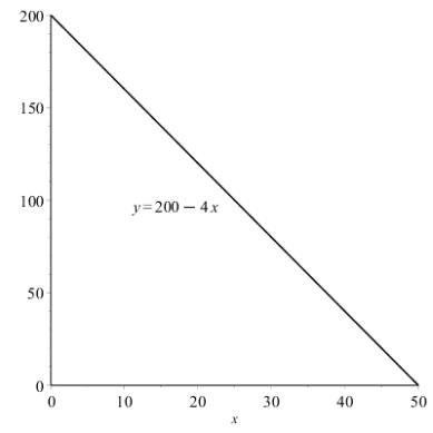
(a) A graph of the model 2004 yx =− is given here:
Solution and Answer Guide: Stewart Kokoska, Calculus: Concepts and Contexts, 5e, 2024, 9780357632499, Chapter 1: Section 1.2
(b) The slope of this line, 4, indicates that each additional dollar charged for rent is predicted to result in a decrease of four spaces rented. This is the rate of change in the number of spaces with respect to the rent charged. The y-intercept ( )0,200 indicates that if nothing is charged, 200 spaces will be rented. The xintercept ( )50,0 indicates that if $50 per space is charged, no spaces will be rented.
1.2.44
(a) Here is a graph of the function:
(b) The slope of this graph is 9/5. The slope indicates that each increase of one degree in the Celsius temperature will result in a 9/5 degree increase in the Fahrenheit temperature. The slope represents the rate of change in the Fahrenheit temperature with respect to the Celsius temperature. The F-intercept is (0,32) and it tells us that a temperature of 0 ℃ is equivalent to 32 ℉.

1.2.45
(a) The driver is driving at a constant rate of ( ) ( ) 40 miles/50 minutes4/5 = mi/min or 48 mi/hr. We can write 48,dt = where d is the distance traveled (in miles) and t is the time (in hours).
(b) A graph of the model 48 dt = is given here:
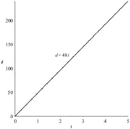
(c) The slope of this line is 48. At this rate, each hour the driver will travel 48 miles.
1.2.46
(a) Using N in place of x and T in place of y , we find the slope to be 21
=== . So a linear equation is ( ) 111731307307 801738051.16 666666
(b) The slope of 1 6 means that the temperature in Fahrenheit degrees increases onesixth as rapidly as the number of cricket chirps per minute. Said differently, each increase of 6 cricket chirps per minute corresponds to an increase of 1F .
(c) When 150 N = , the temperature is given approximately by ( ) 1307 15076.16 F76F 66 T =+= .
1.2.47
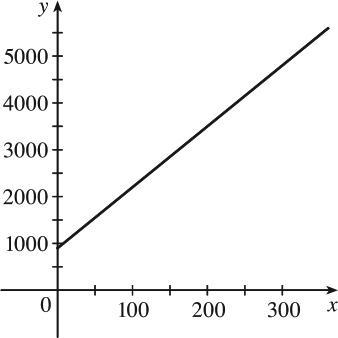
(a) Let x denote the number of chairs produced in one day and y the associated cost. Using the points ( )100,2200 and ( )300,4800 , we get the slope ( ) 480022002600 13.So 220013100 300100200 13900. yx yx
(b) The slope of the line in part (a) is 13 and it represents the cost (in dollars) of producing each additional chair.
(c) The y -intercept is 900 and it represents the fixed daily costs of operating the factory.
Solution and Answer Guide: Stewart Kokoska, Calculus: Concepts and Contexts, 5e, 2024, 9780357632499, Chapter 1: Section 1.2
1.2.48
(a) 0.43415,pd=+ where p = pressure and d = depth below the surface.
(b) The pressure is 100 lb/in2 at a depth of 195.85 ft.
1.2.49
(a) Using d in place of x and C in place of y , we find the slope to be 21 21 460380801 8004803204 CC dd === .
So a linear equation is ( ) 111 460800460200260 444 CdCdCd −=−−=−=+ .
(b) Letting 1500 d = we get ( ) 1 1500260635 4 C =+= .
The cost of driving 1500 miles is $635 .
(c) The slope of the line represents the cost per mile, $0.25 .

(d) The y -intercept represents the fixed cost, $260.
1.2.50
(a) The data appear to be increasing similarly to the values of a cubic function. A model of the form ( ) ( )3 fxaxbc =−+ seems appropriate.
(b) The data appear to be decreasing in a linear fashion. A model of the form ( ) fxmxb =+ seems appropriate.
1.2.51
(a) The data are in the shape of a parabola. A model of the form ( ) ( )2 fxaxbc =−+ seems appropriate.
(b) The data appear to be decreasing similarly to the values of the reciprocal function. A model of the form ( ) / fxax = seems appropriate.
1.2.52
(a) The scatterplot indicates that a linear model would be appropriate.
(b) Using the first and last points we would compute a slope of 8.214.1 0.0001
60,0004000 −
A linear equation for this model would be Ulcer Rate = –0.0001(Income –4000) + 14.1.
(c) The least squares regression equation is Ulcer Rate = –0.0001×Income + 13.95.
(d) The ulcer rate for an income of $25,000 is predicted to be 11.45%.
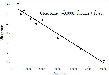
(e) A person with an income of $80,000 is predicted to have a 5.95% chance of peptic ulcers.
(f) An income of $200,000 is quite far from the given income values so it would not be appropriate to apply the model in this case. If the model were applied, the resulting rate would be negative which makes no sense.
1.2.53
a) Graph
(b) The regression equation is Chirp rate = 4.857×Temperature – 221.
(c) The predicted chirping rate for an outdoor temperature of 100 ℉ is 48.57 – 221 = 264.7 chirps per minute.
1.2.54
(a) Graph
(b) The regression equation is Height = 1.881 × Femur Length + 82.65.
(c) A person with a femur 53 cm long is predicted to have been 182.343 cm tall.


Solution and Answer Guide: Stewart Kokoska, Calculus: Concepts and Contexts, 5e, 2024, 9780357632499, Chapter 1: Section 1.2
1.2.55
(a) A linear model seems appropriate over the time interval considered.
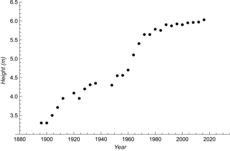
(b) Using a computing device, we obtain the least squares regression line 0.02543.649. y t −

(c) When 2020, t = 6.44, y = which is higher than the actual winning height of 6.02 m.
(d) No, since the times appear to be leveling off (or at least increasing at a lower rate) and getting further away from the model.
1.2.56
(a) The regression equation is Percent Tumors = 0.01879×Asbestos Exposure + 0.305.
(b) The regression line does appear to be a suitable model for the data as the data is fairly linear.
Solution and Answer Guide: Stewart Kokoska, Calculus: Concepts and Contexts, 5e, 2024, 9780357632499, Chapter 1: Section 1.2
(c) The y-intercept, (0, 0.305), indicates that if there is no asbestos exposure then 0.305% of the mice are predicted to develop lung tumors.

1.2.57
(a) A linear model seems appropriate over the time interval considered.

(b) Using a computing device, we obtain the least squares regression line 1.10060.109, y t + where t represents years since 1985.
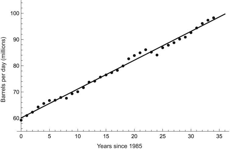
(c) The year 2002 is 17 years after 1985. When 17, t = 78.80. y =
(d) The year 2020 is 35 years after 1985. When 35, t = 98.60, y = which is higher than the 92.2 million barrels per day that the U.S. Energy Information Administration estimates the world consumed.
1.2.58
(a) A linear model seems appropriate over the time interval considered.
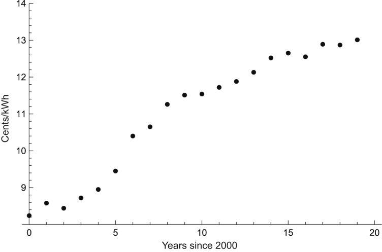
(b) Using a computing device, we obtain the least squares regression line 0.2778.369. t y +

(c) The year 2005 is 5 years after 2000. When 5, t = 9.75. y = The year 2017 is 17 years after 2000. When 17, t = 13.07. y = Using the linear model, we estimate the average retail price of electricity in 2005 as 9.75 cents/kWh and in 2017 as 13.07 cents/kWh. Each estimate is higher than the actual average retail price.
1.2.59
The light would be ( ) 2 1 2 = 4 times brighter.
1.2.60
(a) 0.3 (60)0.7602.39S == so you would expect to find 2 species of bats living in that cave. (b)
1.2.61
(a) 1.499528750 1.000431227 Td = (b) The power model in part (a) is approximately 1.5Td = . Squaring both sides gives us 23Td = , so the model matches Kepler's Third Law, 23Tkd = . 1.2.62
Note that xx =− for 0 x and xx = for 0. x Also, ( )33xx+=−+ for 3 x − and 33xx+=+ for 3. x − Combining these, we have: ( ) ( ) 3323xxxxx ++=−+−+=−− for 3, x − ( ) ( ) 333xxxx ++=−++= for ; 3 0 x and
Solution and Answer Guide: Stewart Kokoska, Calculus: Concepts and Contexts, 5e, 2024, 9780357632499, Chapter 1: Section 1.2
Finally, adding 2 to each resulting expression above gives: 21,3 ()5,30.
Instructor Manual
Instructor Manual: Stewart/Kokoska, Calculus: Concepts & Contexts Fifth Edition, Core 9780357632499; Chapter 2: Limits
PURPOSE AND PERSPECTIVE OF THE CHAPTER
The purpose of this chapter is to explore the concept of limits, motivated by a discussion of the tangent line and instantaneous velocity problems. Limits are treated from descriptive, graphical, numerical, and algebraic points of view. Note that the precise definition of a limit is provided in Appendix D for those who wish to cover this concept. It is important to carefully consider Sections 2.6 and 2.7, which deal with derivatives and rates of change, before the differentiation rules are covered in Chapter 3. The examples and exercises in these sections explore the meanings of derivatives in various contexts.
CHAPTER OBJECTIVES
The following objectives are addressed in this chapter:
02.01 Interpret the slope of the tangent line in the context of a function.
02.02 Analyze the velocity of an abject.
02.03 Explain the meaning of the limit of a function
02.04 Calculate a limit of a function numerically.
02.05 Calculate one-sided limits of functions numerically.
02.06 State the conditions for which the limit of a function does not exist.
02.07 Evaluate limits of functions using limit laws.
02.08 Evaluate limits using direct substitution.
02.09 Solve the problem using the Squeeze Theorem.
02.10 Examine continuity of functions.
02.11 Describe the end behavior of functions using limits at infinity.
02.12 Identify horizontal asymptotes of functions using limits at infinity.
02.13 Interpret the meaning of the derivative of a function.
02.14 Solve applied and mathematical problems using the limits.
02.15 Given the graph of a function, estimate values of the derivative of the function.
02.16 Calculate higher order derivatives of several functions.
Instructor Manual: Stewart/Kokoska, Calculus: Concepts & Contexts Fifth Edition, Core 9780357632499; Chapter 2: Limits
WHAT'S NEW IN THIS CHAPTER
See the Transition Guide for this title for information about what is new to this chapter.
[return to top]
Instructor Manual: Stewart/Kokoska, Calculus: Concepts & Contexts Fifth Edition, Core 9780357632499; Chapter 2: Limits
CHAPTER OUTLINE
The following outline organizes activities (including any existing discussion questions in PowerPoints or other supplements) and assessments by chapter (and therefore by topic), so that you can see how all the content relates to the topics covered in the text.
SECTION 2.1 THE TANGENT AND VELOCITY PROBLEMS (02.01, 02.02)
A. TEACHING TIPS
a. Points to Stress
1. The tangent line viewed as the limit of secant lines.
2. The concepts of average versus instantaneous velocity, described numerically, graphically, and in physical terms.
3. The tangent line as the line obtained by “zooming” in on a smooth function; local linearity.
4. Approximating the slope of the tangent line using slopes of secant lines.
b. Materials for Lecture
• Estimate slopes from discrete data, as in Exercise 5 and 11.


• Illustrate that many functions such as and look locally linear, and discuss the relationship of this property to the concept of the tangent line.


• Estimate the slope of at the point using the graph (perhaps with a graphing calculator), and then numerically. Draw the tangent line to this curve at the indicated point. Do the same for the points and .

ANSWER
• Discuss the phrase “instantaneous velocity.” Ask the class for a definition, such as, “It is the limit of average velocities.” Use this discussion to shape a more precise definition of a limit.
B. CLASS DISCUSSION
• Pose the question, “What does a secant line to a linear function look like?” Find the slope of the line tangent to at various values of , and show that the slope is the same at all of these values.


• Estimate the slopes of tangent lines to at , and 1, first by inspection, then by exploring the graph on a very small region, and then
Instructor Manual: Stewart/Kokoska, Calculus: Concepts & Contexts Fifth Edition, Core 9780357632499; Chapter 2: Limits
numerically by using slopes of secant lines (the limit of the difference quotients). Using these results, graph the function with its tangent lines at , and 1. Notice that the tangent lines intersect the curve more than once; “tangent” applies only to local behavior. If technology is available, zoom in on the curve and tangent line to see that locally they are very close.


• Explore the curve at . Does the tangent line exist?
• Similarly explore


• Draw tangent lines to the curve at and . Notice the difference in the quality of the tangent line approximations.
• Discuss the distance and velocity problem doing sample calculations with discrete data.
Group Work 1: What’s the Pattern?
The students will not be able to do Part 3 from the graph alone, although some will try. After a majority of them are working on Part 3, announce that they can do this numerically.

If they are unable to get Part 6, have them repeat Part 4 for , and again for . ANSWERS 1., 2.


3. , , , 4. is a good estimate.


5. is a good estimate. 6.


Instructor Manual: Stewart/Kokoska, Calculus: Concepts & Contexts Fifth Edition, Core 9780357632499; Chapter 2: Limits
Group Work 2: Slope Patterns
If a group finishes early, have them try to justify the observations made in the last part of Problem 2.
ANSWERS
1.
2.
(a) 0, 0.2, 0.4, 0.6 (b) 11.5
(a) Estimating from the graph gives that the function is increasing for , decreasing for , and increasing for


(b) The slope of the tangent line is positive when the function is increasing, and the slope of the tangent line is negative when the function is decreasing.


(c) The slope of the tangent line is zero somewhere between and , and somewhere between and 3.2. The graph has a local maximum at the first point and a local minimum at the second.
(d) The tangent line approximates the curve worst at the maximum and the minimum. It approximates best at , where the curve is “straightest,” that is, at the point of inflection.
C. GROUP WORK ACTIVITY
GROUP WORK 1, SECTION 2.1 What’s the Pattern?

Consider the function .
1. Carefully sketch a graph of this function on the grid below.


2. Sketch the secant line to between the points with -coordinates and .
3. Sketch the secant lines to between the pairs of points with the followingcoordinates, and compute their slopes: (a) and (b) and (c) and (d) and

4. Using the slopes you’ve found so far, estimate the slope of the tangent line at .
5. Repeat Problem 4 for .
6. Based on Problems 4 and 5, guess the slope of the tangent line at any point , for .

Instructor Manual: Stewart/Kokoska, Calculus: Concepts & Contexts Fifth Edition, Core 9780357632499; Chapter 2: Limits
GROUP WORK 2, SECTION 2.1 Slope Patterns
1.

(a) Estimate the slope of the line tangent to the curve , where = 0, 1, 2, 3. Use your information to fill in the following table:
(b) You should notice a pattern in the above table. Using this pattern, estimate the slope of the line tangent to at the point = 57.5.
2. Consider the function .

(a) On what intervals is this function increasing? On what intervals is it decreasing?
(b) On what interval or intervals is the slope of the tangent line positive? On what interval or intervals is the slope of the tangent line negative? What is the connection between these questions and part (a)?
(c) Where does the slope of the tangent line appear to be zero? What properties of the graph occur at these points?
(d) Where does the tangent line appear to approximate the curve the best? The worst? What properties of the graph seem to make it so?
D. KNOWLEDGE CHECK
• Geometrically, what is “the line tangent to a curve” at a particular point?
ANSWER Answers will vary. Examples:
• The best linear approximation to a curve at a point.
• The result of repeated zooming in on a curve.
• Draw the line tangent to the following curve at each of the indicated points:
Instructor Manual: Stewart/Kokoska, Calculus: Concepts & Contexts Fifth Edition, Core 9780357632499; Chapter 2: Limits
ANSWER
E. HOMEWORK ASSIGNMENT
CORE EXERCISES 4, 5, 9
SAMPLE ASSIGNMENT 4, 5, 9, 11, 14
Instructor Manual: Stewart/Kokoska, Calculus: Concepts & Contexts Fifth Edition, Core 9780357632499; Chapter 2: Limits
SECTION 2.2 THE LIMIT OF A FUNCTION (02.03, 02.04, 02.05)
A. TEACHING TIPS
a. Points to Stress
1. The various meanings of “limit” (descriptive, numeric, graphic), both finite and infinite. Note that the algebraic manipulations are not yet emphasized.
2. The advantages and disadvantages of using a calculator to compute a limit (as in Example 2).
b. Materials for Lecture

• Present the “motivational definition of limit”: We say that if as gets close to , gets close to , and then lead into the definition in the text.


• Discuss Examples 1, 3 and 4. Note that Examples 1 and 3 use numerical evidence to correctly guess a limit’s value, while in Example 4 the numerical data lead us astray.


• Explore the greatest integer function on the interval in terms of left-hand and right-hand limits.
• The “graphing calculator definition of limit” may be covered as a more careful approach to the definition of limit, or as a way of introducing the ε-δ definition from Appendix D: We say that if for any -range centered at there is an -range centered at a such that the graph is entirely contained in the window. The transition to the traditional definition can be made easier by observing that the width of the -range is and the width of the -range is


• Estimate how close must be to 0 to ensure that is within 0.031 of 1. Then estimate how close is to 1 if is within 0.001 of 0. Describe what you did in terms of the relevant definitions of limit.
• Discuss how we can rephrase the last section’s concept as “the slope of the tangent line is the limit of the slopes of the secant lines”.
B. CLASS DISCUSSION


• Explore , looking carefully at from both sides for small Discuss in graphical, numerical, and algebraic (“what happens to when is small?”) contexts.

ANSWER The left-hand limit is 2, because vanishes. The right-hand limit is
Instructor Manual: Stewart/Kokoska, Calculus: Concepts & Contexts Fifth Edition, Core 9780357632499; Chapter 2: Limits


• Discuss either in an context, or using the “graphing calculator definition of limit” described above.

• Go over the estimation of graphically, numerically, and algebraically.
• Discuss a limit such as . When can you “just plug in the numbers”?

Group Work 1: An ‘‘Interesting’’ Function
Introduce this exercise with a review of the concepts of left- and right-hand limits. Also make sure that the students can articulate that when a denominator gets small, the function gets large, and vice versa. (This will be needed for the second question in Parts 2 and 3.) When a group is done, inform them that one of them will be chosen at random to discuss the answer with the class, so all should be able to describe their results. When they graph , they are expected to use graphing technology. When they are all finished, have a different person present the solution to each part.

ANSWERS
1.

2. The limit is 0. When is small and positive, is large and positive, so is large and negative. Therefore its reciprocal is very small and negative, approaching zero.
3. The limit is 1. When is small and negative, is large and negative, and is very close to 1.
4. The limit doesn’t exist because the left- and right-hand limits are not equal.
Instructor Manual: Stewart/Kokoska, Calculus: Concepts & Contexts Fifth Edition, Core 9780357632499; Chapter 2: Limits
Group Work 2: A ‘‘Jittery’’ Function
Introduce this exercise with a good review of the definition of limit. Students find this concept hard, and they will need it to complete this exercise. Make sure to leave time for either you or one of the groups to present a solution. If the students know several definitions of limit, discuss the answer in several ways.
ANSWERS
1.

2. The limit exists and is 0. We can let the values of get as close to 0 as we like by taking sufficiently close to 0. (If limits are covered, then letting will work.)
3. The limit does not exist. There is no value of that will force the values of to remain within 0.1 of 1. (No value of δ will work for .)

4. The limit does not exist if , for the same reason as in Problem 3.

Group Work 3: Limits of Unusual Functions
This exercise asks students to analyze functions with unusual behavior near . The two parts are independent and can be assigned independently of each other.
ANSWERS
1.

(a) Answers will vary; and {1, 0.1, 0.01, 0.001} work.
(b) Both of the sequences above can be extended forever and tend to zero. This does not imply that , because they are carefully chosen -values.

(c)

(d) The limit does not exist.
Instructor Manual: Stewart/Kokoska, Calculus: Concepts & Contexts Fifth Edition, Core 9780357632499; Chapter 2: Limits
2.
(a)
(b) is large negative. (c) is close to zero.
(d)


(e) The limit does not exist: we have a sine whose argument tends to infinity. (f)
Group Work 4: Why Can’t We Just Trust the Table?
This activity was inspired by the article “An Introduction to Limits” from College Mathematics Journal, January 1997, page 51, and extends Example 4. Put the students into groups and give each group two different digits between 1 and 9, and then let them proceed with the problems in the handout.
ANSWERS
1. The answer, of course, depends on the starting digit:
Instructor Manual: Stewart/Kokoska, Calculus: Concepts & Contexts Fifth Edition, Core 9780357632499; Chapter 2: Limits

Instructor Manual: Stewart/Kokoska, Calculus: Concepts & Contexts Fifth Edition, Core 9780357632499; Chapter 2: Limits
2. Answers will vary.
3. Answers will vary. 4. There is no limit
Instructor Manual: Stewart/Kokoska, Calculus: Concepts & Contexts Fifth Edition, Core 9780357632499; Chapter 2: Limits
C.
GROUP WORK ACTIVITY
GROUP WORK 1, SECTION 2.2 An ‘‘Interesting’’ Function
1. Create a graph of the function .


2. Estimate from the graph. Back up your estimate by looking at the function, and discussing why your estimate is probably correct.
3. Estimate from the graph. Back up your estimate by looking at the function, and discussing why your estimate is probably correct.
4. Does exist? Justify your answer.

Instructor Manual: Stewart/Kokoska, Calculus: Concepts & Contexts Fifth Edition, Core 9780357632499; Chapter 2: Limits
GROUP WORK 2, SECTION 2.2 A ‘‘Jittery’’ Function
Not all functions that occur in mathematics are simple combinations of the standard functions usually seen in calculus. Consider this function:

1. It is obvious that you can’t graph this function in the same, literal way that you would graph . But it is useful to have some idea of what this function looks like. Try to sketch the graph of .


2. Do you believe that exits? If so, what is its value? Give reasons for your answer.
3. Does exist? Carefully justify your answer.

4. What do you conjecture about if ?
GROUP WORK 3, SECTION 2.2 Limits for Unusual Functions
1. Consider the function . We wish to investigate the behavior of this function near .


(a) Find four values of x for which . Hint: Remember that if is an integer.
(b) Explain why there is an infinite set of values of tending to 0 for which . Does this imply that ? Why or why not?

(c) In a fashion similar to that of part (b), find an infinite set of values of for which

(d) In light of part (c), what can you now say about ?
(e) Show how the graph of verifies your answers to the previous parts.
Instructor Manual: Stewart/Kokoska, Calculus: Concepts & Contexts Fifth Edition, Core 9780357632499; Chapter 2: Limits
2. Now consider

(a) What is the range of ?

(b) If is close to 0 and negative, what can you say about the value of ?
(c) If is very large and negative, what can you say about ?

(d) Use your answers to parts (b) and (c) to help you compute . What is ?

(e) What do you predict will happen when you use these same steps to try to compute ? Give reasons for your answers.

(f) Examine a graph of near . Does this graph look like what you expected?
GROUP WORK 4, SECTION 2.2 Why Can’t We Just Trust the Table?

We are going to investigate We will take values of x closer and closer to zero, and see what value the function approaches.
1. Your teacher has given you a digit let’s call it d. Fill out the following table. If, for example, your digit is 3, then you would compute etc.

Instructor Manual: Stewart/Kokoska, Calculus: Concepts & Contexts Fifth Edition, Core 9780357632499; Chapter 2: Limits
x 0.d 0.0d 0.00d 0.000d 0.0000d 0.00000d
2. What is ?
3. Now fill out the table with a different digit. x 0.d 0.0d 0.00d 0.000d 0.0000d 0.00000d
Do you get the same result?
4. What is ?
D. KNOWLEDGE CHECK


• What is the difference between the statements and ?
ANSWER The first is a statement about the value of f at the point , the second is a statement about the values of at points near, but not equal to, .
• Why is it the case that your calculator shows if is very small?

ANSWER If is small enough, underflow will cause the calculator to represent as exactly zero.

Instructor Manual: Stewart/Kokoska, Calculus: Concepts & Contexts Fifth Edition, Core 9780357632499; Chapter 2: Limits
E. HOMEWORK ASSIGNMENT
CORE EXERCISES 1, 6, 18, 39
SAMPLE ASSIGNMENT 1, 2, 3, 6, 11, 18, 34, 37, 39
Instructor Manual: Stewart/Kokoska, Calculus: Concepts & Contexts Fifth Edition, Core 9780357632499; Chapter 2: Limits
SECTION 2.3 CALCULATING LIMITS USING THE LIMIT LAWS (02.06,
02.07,
02.08, 02.09)
A. TEACHING TIPS
a. Points to Stress
1. The algebraic computation of limits: manipulating algebraically, examining leftand right-hand limits, using the limit laws to break monstrous functions into pieces, and analyzing the pieces.
2. The evaluation of limits from graphical representations.
3. Examples where limits don’t exist (using algebraic and graphical approaches).
4. The computation of limits when the limit laws do not apply.
b. Materials for Lecture

• Discuss why is not a straightforward application of the Product Law.

ANSWER does not exist.

• Compute some limits of quotients, such as and always attempting to plug values in first.

ANSWER The second and third can be computed just by plugging in the values. , and


• Do some subtle product and quotients, such as and . ANSWER and by rationalizing the numerator.


• If the group exercise “A ‘Jittery’ Function” was assigned in Section 2.2, use the Squeeze Theorem to show that . Show what happens when we try to compute the limit at another point, such as , and show why the Squeeze Theorem doesn’t apply in that case.

Instructor Manual: Stewart/Kokoska, Calculus: Concepts & Contexts Fifth Edition, Core 9780357632499; Chapter 2: Limits
• If the group exercise “A ‘Jittery’ Function” was not assigned in Section 2.2, use the Squeeze Theorem to show that by squeezing between and 0.

B. CLASS DISCUSSION


• Have the students check if exists, and then compute left- and right-hand limits. Then check


ANSWER does not exist. The left-hand limit is and the righthand limit is 1.

• Present some graphical examples, such as and in the graph below
ANSWER


• Have the students determine the existence of and determine why we cannot compute . ANSWER x can never be less than zero, so there is no left-hand limit.
Instructor Manual: Stewart/Kokoska, Calculus: Concepts & Contexts Fifth Edition, Core 9780357632499; Chapter 2: Limits

• Compute some limits of quotients, such as and always attempting to plug values in first.
ANSWER The second and third can be computed just by plugging in the values , and .
Group Work 1: Exploring Limits
Have the students work on this exercise in groups. Problem 2 is more conceptual than Problem 1, but makes a very important point about the sums and products of limits.
ANSWERS
1.
(a) (i) Does not exist
(ii) Does not exist
(iii) 4
(iv) Does not exist
(b) (i) Does not exist
(ii) 1
(c) (i) 0
(ii) Does not exist 2.
(a) Both quantities exist. (b) Each quantity may or may not exist.
Group Work 2: The Squeeze Theorem

Review the definition of before beginning this exercise. Part A of this group work computes both graphically and using the Squeeze Theorem. As a followup activity, have the students compute using the Squeeze Theorem. Exercises 1 and 2 can be used if the students need practice on the Squeeze Theorem, or if you are running out of time. Part B gives an informal graphical way to show that . A more careful geometric argument is given in Section 3.3.


C. GROUP WORK ACTIVITY
GROUP WORK 1, SECTION 2.3 Exploring Limits
1. Given the functions and (defined graphically below) and and (defined algebraically), compute each of the following limits, or state why they don’t exist:
or
Instructor Manual: Stewart/Kokoska, Calculus: Concepts & Contexts Fifth Edition, Core 9780357632499; Chapter 2: Limits


(a) (i) (ii) (iii) (iv) (b) (i) (ii) (c) (i) (ii)


2.


(a) In general, if exists and exists, is it true that exists? How about ? Justify your answers.


(b) In general, if does not exist and does not exist, is it true that does not exist? How about ? Compare these with your answers to part (a).
Instructor Manual: Stewart/Kokoska, Calculus: Concepts & Contexts Fifth Edition, Core 9780357632499; Chapter 2: Limits
GROUP WORK 2, SECTION 2.3 The Squeeze Theorem
PART A


1. Let . Why is it clear that ?

2. Let , where is the greatest integer less than or equal to u. We want to compute .


(a) Suppose . Show that , and hence .


(b) Suppose . Show that , and hence .

(c) Suppose . Guess a formula for and show that it is correct.

(d) Suppose is an integer and . Guess a formula for . Can you show that it is correct?

(e) Draw a graph of for . On the basis of this graph, what is ?

3. Using a graphing calculator or computer, show that if
4. Can you use this inequality to compute ?
PART B
In this part, we take a graphical approach to computing .


1. Using a graphing calculator, show that if , then . Give a rough sketch of the three functions over the interval on the graph below.


Instructor Manual: Stewart/Kokoska, Calculus: Concepts & Contexts Fifth Edition, Core 9780357632499; Chapter 2: Limits


2. Again using a graphing calculator, show that if , then . If you have not done so already, add these portions of the three functions to your graph above.

3. Using the inequalities in Exercises 1 and 2, why is for ?

4. Again using Exercise 7, can you find a function with on such that ?

5. Using Exercises 3 and 4, compute .
D. KNOWLEDGE CHECK

• When can and can’t you evaluate a limit just by plugging in the relevant value of ?
ANSWER You can’t, for example, when there is a zero in the denominator, when you are at the border of a piecewise function, and so forth.
• In Example 1, why does not exist?
E. HOMEWORK ASSIGNMENT

CORE EXERCISES 1, 2, 30, 37, 39, 63
SAMPLE ASSIGNMENT 1, 2, 6, 30, 37, 39, 40, 44, 49, 63, 66
Instructor Manual: Stewart/Kokoska, Calculus: Concepts & Contexts Fifth Edition, Core 9780357632499; Chapter 2: Limits
SECTION 2.4 CONTINUITY (2.10)
A. TEACHING TIPS
a. Points to Stress
1. The geometric and mathematical definitions of continuity.
2. Examples of discontinuity.
3. The Intermediate Value Theorem: mathematical statement, graphical examples, applied examples.
b. Materials for Lecture
• Discuss the idea of continuity at a point, continuity on an interval, and the basic types of discontinuities.
• Note that the statement “ is continuous at ” is implicitly saying three things:
1. exists

2. exists.
3. The two quantities are equal.
To show that all three statements are important to continuity, have the students come up with examples where the first holds and the second does not, the second holds and the first does not, and where the first two hold and the third does not. Examples are sketched below.


• Compare two functions such as and at in order to show the difference between removable and non-removable discontinuities.
• Some students tend to believe that at all piecewise functions are discontinuous at the border points. Examine the function at the points and . This would be a good time to point out that the function is continuous everywhere, including at .


Instructor Manual: Stewart/Kokoska, Calculus: Concepts & Contexts Fifth Edition, Core 9780357632499; Chapter 2: Limits
• Start by stating the basic idea of the Intermediate Value Theorem (IVT) in broad terms. (Given a function on an interval, the function hits every y-value between the starting and ending y-values.) Then attempt to translate this statement into precise mathematical notation. Show that this process reveals some flaws in our original statement that have to be corrected (the interval must be closed; the function must be continuous.)
• To many students the IVT says something trivial to the point of uselessness. It is important to show examples where the IVT is used to do non-trivial things.
EXAMPLE A graphing calculator uses the IVT when it graphs a function. A pixel represents a starting and ending y-value, and it is assumed that all the intermediate values are there. This is why graphing calculators are notoriously bad at graphing discontinuous functions.
EXAMPLE Assume a circular wire is heated. The IVT can be used to show that there exist two diametrically opposite points with the same temperature.
ANSWER Let be the difference between the temperature at a point x and the temperature at the point opposite x. f is a difference of continuous functions, and is thus continuous itself. If , then , so by the IVT there must exist a point at which


EXAMPLE Show that there exists a number whose cube is one more than the number itself. (This is Exercise 70.)

ANSWER Let . is continuous, and and . So by the IVT, there exists an with
B. CLASS DISCUSSION
• Do Exercise 3 as an example, or revisit Exercise 9 in Section 2.2.
• Consider . Discuss where this function is continuous.

Point out that there are different types of discontinuities at and .


• Indicate why is continuous everywhere on its domain, but is not continuous everywhere. Then discuss the continuity of , and why all the discontinuities of g are now removable.
• If the group work “A ‘Jittery’ Function” was assigned, revisit
Ask the students to guess if this function is continuous at . Many will not believe that it is. Now look at it using the definition of continuity. They should agree that . In the group work it was shown that existed and was equal to 0. So, this function is continuous at . A sketch such as the one below may be helpful.
Instructor Manual: Stewart/Kokoska, Calculus: Concepts & Contexts Fifth Edition, Core 9780357632499; Chapter 2: Limits

• Present the following scenario: two ice fishermen are fishing in the middle of a lake. One of them gets up at 6:00 P.M. and wanders back to camp along a scenic route, taking two and a half hours to get there. The second one leaves at 7:00 P.M., and walks to camp along a direct route, taking one hour to get there. Show that there was a time where they were equidistant from camp.

ANSWER Start by superimposing two possible position versus time graphs. Let be the difference between the two fishermen’s positions, and invoke the IVT to prove that the graphs cross.
Group Work 1: Exploring Continuity

Warm the students up by having them graph without their calculators, and asking where it is continuous. The first problem is appropriate for all classes. Problem 2 assumes the students have previously seen the activity “A ‘Jittery’ Function”. If they have not, skip it and go directly to Problem 3. Before handing out Problem 3, make sure that the students recall the definition of the greatest integer (“floor”) function . After this exercise, discuss the continuity of at integer and at non-integer values. Problem 4 is intended for classes with a more theoretical bent.

ANSWERS
1. c = 4, m = 5 2.
(b) 0
(c) 0
(d) It is continuous because 3.


Instructor Manual: Stewart/Kokoska, Calculus: Concepts & Contexts Fifth Edition, Core 9780357632499; Chapter 2: Limits
(a)
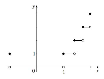
(b) All values except


(c) does not exist because the left- and right-hand limits are different.
4.

(a) The fact that is continuous implies that for all a. Then, by the Limit Laws, .
(b) False. For example, let

Group Work 2: The Area Function
This activity is designed to reinforce the notion of continuity by presenting it in an unfamiliar context. It will also ease the transition to area functions in Chapter 5. It is important that this activity be well set up. Do Problem 1 with the students, making sure to compute a few values of and to sketch it. The students should try to answer Problems 1 and 2 using their intuition and the definition of continuity. It may be desirable to have the students restrict themselves to . Note that in this exercise, one can “prove” continuity by looking at the actual formulas for and , but that the goal of the exercise is that the students understand intuitively why both area functions are continuous.


Students may disagree on the answer to Problem 3. If you are fortunate enough to have groups that have reached opposite conclusions, break up one or more of them, and have representatives go to other groups to try to convince them of the error of their ways.


ANSWER Yes to all three questions. For all , and exist; , and . (The limits can be shown to exist by looking at the left and right-hand limits.)
Instructor Manual: Stewart/Kokoska, Calculus: Concepts & Contexts Fifth Edition, Core 9780357632499; Chapter 2: Limits
Group Work 3: The Twin Problem
When students see this problem, there is a good chance that they will disagree among themselves about the answer. Let them argue for a while. Ideally, they will come up with the idea of using the Intermediate Value Theorem to prove that Dr. Stewart was correct. If they don’t, this may need to be given to them as a hint. Another hint they may need is that the Intermediate Value Theorem deals with a single continuous function, whereas the problem is talking about two functions, Stewart’s temperature and Shasta’s temperature. They will have to figure out a way to find a single function that they can use. Encourage them to write up a solution to the exact degree of rigor that will be expected of them on homework and exams; this is a good opportunity to convey the course’s expectations to the students.


ANSWER Let and be Dr. Stewart’s and Shasta’s temperatures at time t. Now let is continuous (being a difference of continuous functions), (Dr. Stewart is warmer at first), and (where f represents the end of the vacation; Shasta is warmer at the end). Therefore, by the ivt, there exists a time a at which and hence . Notice that most students who try to argue that the conclusion is false (using things such as stasis chambers and speeds in excess of ) are really trying to construct a scenario in which the continuity of the temperature function is violated.
Group Work 4: Swimming to the Shore
Emphasize to the students that they are not trying to find x, but simply trying to prove its existence. As in the Twin Problem, a first hint might be to use the IVT, and a second could be to find a single continuous function of . It is probably best to do this activity after the students have seen the solution to the ice fisherman problem above, or the Twin Problem.


ANSWER Let . is continuous, , and . Therefore, by the IVT, there is a place where
C. GROUP WORK ACTIVITY

GROUP WORK 1, SECTION 2.4 Exploring Continuity

1. Are there values of c and that make continuous at ? Find c and , or explain why they do not exist.
2. Recall the function
Instructor Manual: Stewart/Kokoska, Calculus: Concepts & Contexts Fifth Edition, Core 9780357632499; Chapter 2: Limits

(a) It is obvious that you can’t graph this function in the same, literal way that you would graph . But it is useful to have some idea of what this function looks like. Try to sketch the graph of .
(b) Do you believe that is continuous at ? Why or why not?
(c) What is ?
(d) What is ?
(e) Use parts (c) and (d) either to revise your answer to part (b), or to prove that your answer is correct.
3. Consider the function

(a) Sketch the graph of the function for .


(b) For what values of , is ?

(c) Compute and , if they exist. Explain your answers.
Instructor Manual: Stewart/Kokoska, Calculus: Concepts & Contexts Fifth Edition, Core 9780357632499; Chapter 2: Limits
GROUP WORK 2, SECTION 2.4
The Area Function
The following are graphs of and :

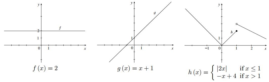
1. Let be the area enclosed by the -axis, the -axis, the graph of the function , and the line . Would you conjecture that is continuous at every point in the domain of ? Why or why not?
2. Let be the area enclosed by the -axis, the -axis, the graph of the function g, and the line . Would you conjecture that is continuous at every point in the domain of ? Why or why not?
3. Let be the area enclosed by the -axis, the -axis, the graph of the function h, and the line . Would you conjecture that is continuous at every point in the domain of h? Why or why not?
GROUP WORK 3, SECTION 2.4
The Twin Problem
There is a bit of trivia about the author of your textbook, Dr. James Stewart, that very few people know. He has an evil twin sister named Shasta. Although he loves his sister dearly she dislikes him, and tries to be different from him in all things. Last winter, they both went on vacation. Dr. Stewart went to Hawaii. Shasta had planned on going to Aruba, but she decided against it. She hates her brother so much that she was afraid there would be a chance that they might be experiencing the same temperature at the same time, and that prospect was distasteful to her. So she decided to vacation in northern Alaska.
After a few days, Dr. Stewart received a call: “This is Shasta. I am very cold and uncomfortable here. That’s good, since you are undoubtedly warm and comfortable, and I want us to be different. But I’m not sure why I should be the one in northern Alaska. I think we should switch places for the last half of our trip.”
“It is only fair,” he agreed.
Instructor Manual: Stewart/Kokoska, Calculus: Concepts & Contexts Fifth Edition, Core 9780357632499; Chapter 2: Limits
So they each traveled again. Dr. Stewart took a trip from Hawaii to Alaska, while Shasta took a trip from Alaska to Hawaii. They each traveled their own different routes, perhaps stopping at different places along the way. Eventually, they had reversed locations. Dr. Stewart was shivering in Alaska, Shasta was in Hawaii, warm and happy. She received a call from her brother.
“Hi, Shasta. Guess what? At some time during our travels, we were experiencing exactly the same temperature at the same time. So Ha!”
Is Dr. Stewart right? Has Good triumphed over Evil? He would try to write out a proof of his statement, but his hands are too frozen to grasp his pen. Help him out. Either prove him right, or prove him wrong, using mathematics.
GROUP WORK 4, SECTION 2.4
Swimming to the Shore


A swimmer crosses a river starting at point and ending at point , following the path shown below. Prove that for some value , the swimmer’s distance from is the same as the distance from .
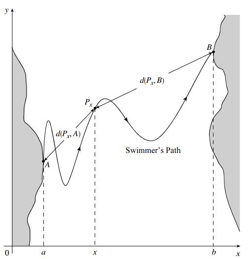
Instructor Manual: Stewart/Kokoska, Calculus: Concepts & Contexts Fifth Edition, Core 9780357632499; Chapter 2: Limits
D. KNOWLEDGE CHECK
• Is it possible for a function to be continuous from the right at and continuous from the left at , but not continuous at ? Why or why not?

ANSWER No. If were continuous from the right and from the left at a, then we would have , and therefore would exist and be equal to


• The text says that is discontinuous at . This would seem to contradict Theorem 7. Does it? Why or why not?
ANSWER It does not; is indeed continuous at every point in its domain, but is not in its domain.
E. HOMEWORK ASSIGNMENT
CORE EXERCISES 2, 4, 7, 11(a), 10(b), 21, 26, 44, 48
SAMPLE ASSIGNMENT 1, 2, 4, 6, 7, 11(a), 10(b), 21, 22, 26, 32, 35, 39, 41, 44, 45, 48
Instructor Manual: Stewart/Kokoska, Calculus: Concepts & Contexts Fifth Edition, Core 9780357632499; Chapter 2: Limits
SECTION 2.5 LIMITS INVOLVING INFINITY (02.11, 02.12)
A. TEACHING TIPS
a. Points to Stress
1. The geometric and limit definitions of asymptotes, particularly as they pertain to rational functions.
2. The computation of infinite limits.
3. The technique, and the dangers, of using calculators to check limits (both numerically and graphically).
b. Materials for Lecture
• Describe asymptotes verbally and then give graphical and limit definitions. Note that a function can cross its horizontal asymptote. Perhaps include a description of slant asymptotes.


• Compute the limits of as and as . Graph the function, showing both discontinuities and end behavior.


ANSWER The limit is 0 as , as , and does not exist as .


• Compute .
ANSWER


. One can argue that as gets large, or one can look at the graph.
Instructor Manual: Stewart/Kokoska, Calculus: Concepts & Contexts Fifth Edition, Core 9780357632499; Chapter 2: Limits


• Graph , after calculating limits as and as .

ANSWER does not exist.

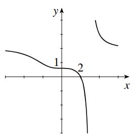
• Calculate . Show the students how to find a domain for such that for all in that domain.

ANSWER

• Examine and . ANSWER does not exist; .
B. CLASS DISCUSSION


• Explore and near
• Do an example similar to Example 4, computing limits at , this time using .

• Ask students if a function can be bounded but not have a horizontal asymptote. Does have a horizontal asymptote? What about ? How is different?


Instructor Manual: Stewart/Kokoska, Calculus: Concepts & Contexts Fifth Edition, Core 9780357632499; Chapter 2: Limits
ANSWER Both and are bounded, but have no asymptote because does not exist. has the -axis as asymptote because


• Examine on a graphing calculator, first by plugging in large numbers, then by examining the graph. Then show that this limit is, in fact, infinity. If teaching a very advanced class, one might try to “prove” that this limit is the expected 5.429 using epsilons and deltas, and see how the attempt fails. [Note: 5.429 is , which is what a student would come up with by plugging very large numbers into a calculator.]
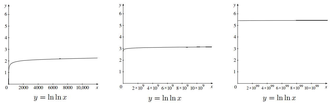
• Compute the domain and determine the limiting behavior, including asymptotes, for

. Note that the asymptotes at and are different.
Instructor Manual: Stewart/Kokoska, Calculus: Concepts & Contexts Fifth Edition, Core 9780357632499; Chapter 2: Limits
Group Work 1: Infinite Limits
This exercise is too long to be done in a 50-minute session. Pick and choose problems. It is more important to have good introduction and closure on each problem than to have all of them worked out. Problem 4 is an extension of Exercise 76
ANSWERS
1. Answers will vary
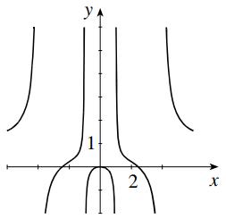
2. Vertical: , horizontal:


3. Answers will vary. Possible answers: (a) (b) (c) (d)
4. (a) (b) 0 (c) or

Instructor Manual: Stewart/Kokoska, Calculus: Concepts & Contexts Fifth Edition, Core 9780357632499; Chapter 2: Limits
Group Work 2: I Am the Greatest
Before handing this exercise out, make sure the students know the definition of the greatest integer function, and can sketch its graph.
ANSWERS

1. This can be done from the graph, or using the definition. (Choose , then let ).

2. (a)

(b) Lower bound , upper bound 1.

(c) Use the Squeeze Theorem, taking the limits of the bounds as .
3. 0
4. When


5. This can be seen by a similar bounding argument to the one above. If you use this exercise, it is a good idea to show the graph to your students, for it is a truly pretty thing:
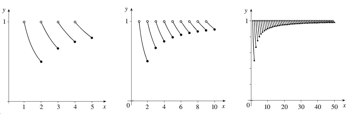
Instructor Manual: Stewart/Kokoska, Calculus: Concepts & Contexts Fifth Edition, Core 9780357632499; Chapter 2: Limits
The tops of the lines are at and the bottoms trace out the curve
C. GROUP WORK ACTIVITY


GROUP WORK 1, SECTION 2.5 Infinite Limits

1. Draw an even function which has the lines , and among its asymptotes.
2. Describe all vertical and horizontal asymptotes of .


3. Find formulas for two functions, and , such that and (a) (b) (c) (d)

4. Let and be polynomials of degree and respectively.

(a) Find if (b) Find if (c) Find if .
1. Show that
GROUP WORK 2, SECTION 2.5 I Am the Greatest
or
(a) Sketch a graph of on the axes below.

2.
Instructor Manual: Stewart/Kokoska, Calculus: Concepts & Contexts Fifth Edition, Core 9780357632499; Chapter 2: Limits


(b) If find upper and lower bounds for the expression .

(c) Use the estimates above to show that .

3. Compute .
4. Show that
5. Compute . Justify your reasoning.

D. KNOWLEDGE CHECK


• If , what can we say about ?
ANSWER It is either , or something in between, or it may not exist at all! In other words, we can say nothing.

• Why are all lines , an integer, vertical asymptotes for Where does the term come from?


• To evaluate the limit at infinity of a rational function, we first divide both the numerator and denominator by the highest power of that occurs in the denominator. Why must we do such a thing?
ANSWER By doing this division, we make the denominator approach a finite value as . Now we can take the limit of the numerator, and easily divide it by the limit of the denominator.
Instructor Manual: Stewart/Kokoska, Calculus: Concepts & Contexts Fifth Edition, Core 9780357632499; Chapter 2: Limits
E. HOMEWORK ASSIGNMENT
CORE EXERCISE 1, 3, 7, 17, 41, 58, 76
SAMPLE ASSIGNMENT 1, 2, 3, 4, 5, 7, 13, 14, 17, 41, 48, 54, 58, 76, 79
Instructor Manual: Stewart/Kokoska, Calculus: Concepts & Contexts Fifth Edition, Core 9780357632499; Chapter 2: Limits
SECTION 2.6 DERIVATIVES AND RATES OF CHANGE (02.13,02.14)
A. TEACHING TIPS
a. Points to Stress
1. The slope of the tangent line as the limit of the slopes of secant lines (graphically, numerically, algebraically).
2. The instantaneous rate of change as the limit of average rates of change.
3. The derivative notations and


4. The units of .
b. Materials for Lecture
• Review the geometry of the tangent line, and the concept of “locally linear”.


• Estimate the slope of the line tangent to at (1, 2) by looking at the slopes of the lines between and and , and so forth. Illustrate these secant lines on a graph of the function, redrawing the figure when necessary to illustrate the “zooming in” process.

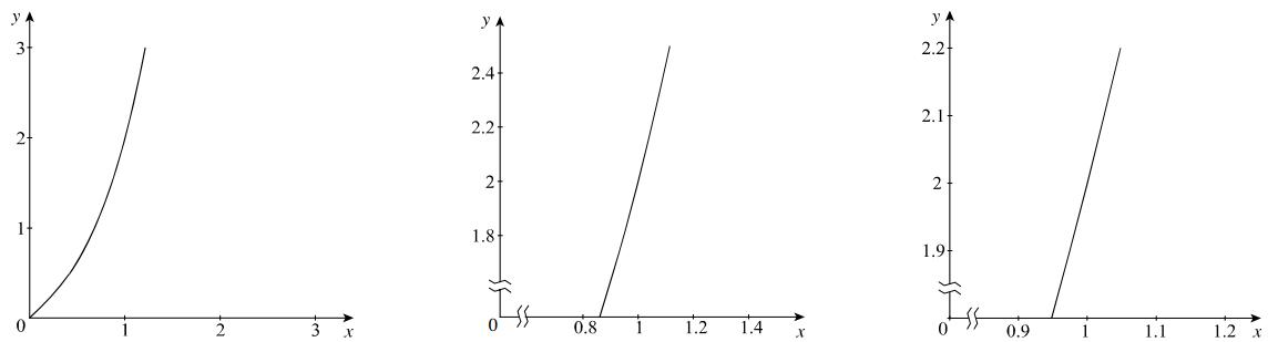
Similarly examine at (0, 1).

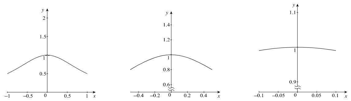
Instructor Manual: Stewart/Kokoska, Calculus: Concepts & Contexts Fifth Edition, Core 9780357632499; Chapter 2: Limits
ANSWER Approximately 4, approximately 0
• Using the curve below, have the students identify values and for such that (where and are the slopes of the tangent lines and ).


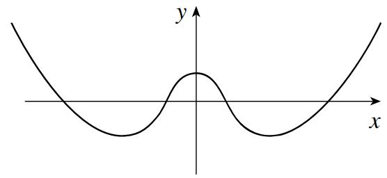
ANSWER There are many correct choices for a and b. One such pair is shown below

• If “A ‘Jittery’ Function” was covered in Section 2.2, look at

Poll the class: Is there a tangent line at ? Then examine what happens if you look at the limits of the secant lines. Note that this is not the same function as the one from the Group Work! That function does not have a tangent line at .


ANSWER The line is tangent to this curve at .
• Note that the text shows that if , then . Thus, and . Demonstrate that these quantities cannot be easily estimated from a graph of the function. Foreshadow the treatment of a as a variable in Section 2.7.
• Draw a figure like the following (or copy it as an overhead) and draw in the secant lines between points and and . Demonstrate how the slope of the tangent line at is the limit of the slopes of the secant lines.


Instructor Manual: Stewart/Kokoska, Calculus: Concepts & Contexts Fifth Edition, Core 9780357632499; Chapter 2: Limits

ANSWER The slopes of the secant lines range from about 1 to about 2.5.
B. CLASSS DISCUSSION

• Have students estimate the slope of the tangent line to at various points. Foreshadow the concept of concavity by asking them some open-ended questions such as the following: What happens to the function when the slope of the tangent is increasing? Decreasing? Zero? Slowly changing?
ANSWER This will be their introduction to concavity, even if the word isn’t used. Increasing slope is concave up, decreasing slope is concave down, changing slowly means the curve looks more linear, changing quickly means the curve looks less linear.
• Consider the velocity function of a car, described by the graph below.
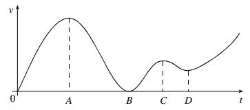
1. Ask the students to determine when the car was stopped.
2. Ask the students when the car was accelerating (that is, when the velocity was increasing). When was the car decelerating?


3. Ask the students to describe what is happening at times , and in terms of both velocity and acceleration. What is happening at time B?
ANSWER
1. The car was stopped at 0 and at B


2. Accelerating for , and , decelerating for and .

3. At A, C, and D, the velocity has a local maximum or minimum (the students might not know these words, but the concepts should be introduced) and the acceleration is zero. At time B the car is stopped, and the acceleration is zero.
Instructor Manual: Stewart/Kokoska, Calculus: Concepts & Contexts Fifth Edition, Core 9780357632499; Chapter 2: Limits
• Note that if a car is driving along a curve, the headlights point in the direction of the tangent line.

• Draw a function like the following, and first estimate slopes of secant lines between and , and between and . Then order the five quantities and in decreasing order.


ANSWER
• Draw a function like the following and ask the students to find points and such that . Then ask them to find and such that


• Derive at if

• “Thumbnail” derivative estimates: Graph a function on the board and have the class call out rough values of the derivative. Is it larger than 1? About 1? Between 0 and 1? About 0? Between and 0? About ? Smaller than ?
Instructor Manual: Stewart/Kokoska, Calculus: Concepts & Contexts Fifth Edition, Core 9780357632499; Chapter 2: Limits
Group Work 1: Follow That Car
Start this problem by giving the students the function and having them sketch its graph. Ask them how far the car has traveled after 1, 2, and 3 hours, and then show them how to compute the average velocity for [0, 1], [1, 2], and [2, 3].
ANSWERS
1.
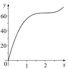
2. It appears to stop at .
3.


4. . This is where the car stops.
Group Work 2: Order from Chaos
Have the students work on this exercise in groups of three or four. Some groups may try to solve the problems by estimating the relevant quantities numerically, and others will use geometric arguments. For the purposes of this assignment, both approaches are equally valid.
ANSWERS
1. 2.
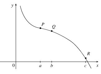
Instructor Manual: Stewart/Kokoska, Calculus: Concepts & Contexts Fifth Edition, Core 9780357632499; Chapter 2: Limits
Group Work 3: Connect the Dots
Closure is very important on this exercise. At this point in the course, many students will have the impression that all reasonable estimates are equally valid, so it is crucial that students discuss Problem 4. If there is student interest, this table can generate a rich discussion. Can ever be negative? What would that mean in real terms? What would mean in real terms in this instance?


ANSWERS
1. It is likely to be an overestimate, because the function is concave down at .

2. After spending $3500, consumer approval is increasing at the rate of about 0.06 % for every additional dollar spent.
3. Percent per dollar
4. This is a better estimate because the same figures now give a two-sided approximation of the limit of the difference quotient.
Group Work 4: Derivatives and Inverses
If inverse functions were covered, this exercise is an excellent way for students to synthesize the two concepts, and to gain intuition and understanding about what the derivative means in a real-world context.
ANSWERS

1. is the time at which a given number of centimeters of rain have fallen. The domain is from 0 cm to the maximum total rainfall. The range is from midnight to the end of the storm.
2.
(a) At 5:00 A.M., 2 cm of rain has fallen.
(b) 5 cm of rain has fallen at 2:00 A.M.
(c) At 5 A.M., the rain is falling at the rate of 0.5 cm/h.
(d) After 5 cm of rain has fallen, time is passing at a rate of one half hour per centimeter of rainfall.
C. GROUP WORK ACTIVITY
GROUP WORK 1, SECTION 2.6 Follow That Car
Here, we continue with the analysis of the distance of a car, where d is in miles and t is in hours.

2. Does the car ever stop?

1. Draw a graph of from to .

3. What is the average velocity over ? over ? over ?
or
or
Instructor Manual: Stewart/Kokoska, Calculus: Concepts & Contexts Fifth Edition, Core 9780357632499; Chapter 2: Limits
4. Estimate the instantaneous velocity at . Give a physical interpretation of your answer.
GROUP WORK 2, SECTION 2.6 Order from Chaos
Below is the graph of the function .
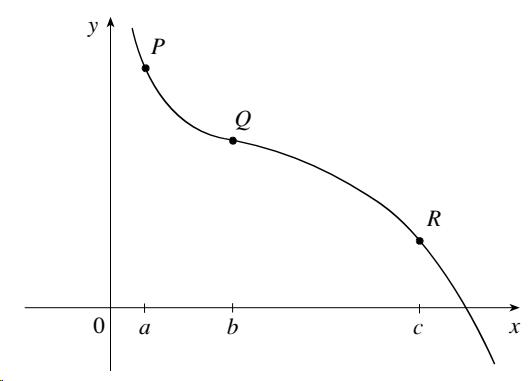

1. Place the following quantities in order, from lowest to highest: , the slope of the secant line PQ, the slope of the secant line QR, and . Make sure to give justification for your answers.

2. Find points P, Q, and R as above such that and

GROUP WORK 3, SECTION 2.6 Connect the Dots
A company does a study on the effect of production value p of an advertisement on its consumer approval rating A. After interviewing eight focus groups, they come up with the following data:
Assume that gives the consumer approval percentage as a function of p.
or

1. Estimate . Is this likely to be an overestimate or an underestimate?

2. Interpret your answer to Problem 1 in real terms. What does your estimate of tell you?
3. What are the units of ?
Instructor Manual: Stewart/Kokoska, Calculus: Concepts & Contexts Fifth Edition, Core 9780357632499; Chapter 2: Limits
4. Estimate . Is your estimate better or worse than your estimate of ? Why?
GROUP WORK 4, SECTION 2.6 Derivatives and Inverses
Let be the number of centimeters of rainfall that has fallen on my porch since midnight, where t is the time in hours.
1. Describe the inverse function in words. What are the domain and range of ?


2. Interpret the following in practical terms. Include units in your answers. (a) (b) (c) (d)


D. KNOWLEDGE CHECK
• What is meant by the terms “tangent line” and “secant line”?
• Why is it necessary to take a limit when computing the slope of the tangent line?
ANSWER There are several possible answers here. Examples include the following:
• By definition, the slope of the tangent line is the limit of the slopes of secant lines.
• You don’t know where to draw the tangent line unless you pick two points very close together. The idea is to get them thinking about this question.
Instructor Manual: Stewart/Kokoska, Calculus: Concepts & Contexts Fifth Edition, Core 9780357632499; Chapter 2: Limits
E. HOMEWORK ASSIGNMENT
CORE EXERCISES 1, 5, 12, 15, 19, 29, 34, 54, 62
SAMPLE ASSIGNMENT 1, 3, 4, 5, 11, 12, 14, 15, 16, 19, 28, 29, 33, 34, 37, 41, 54, 62, 63
Instructor Manual: Stewart/Kokoska, Calculus: Concepts & Contexts Fifth Edition, Core 9780357632499; Chapter 2: Limits
SECTION 2.7 THE DERIVATIVES AS A FUNCTION (02.15, 02.16)
A. TEACHING TIPS
a. Points to Stress
1. The concept of a differentiable function, interpreted graphically, algebraically, and descriptively.

2. Obtaining the derivative function by first considering the derivative at a point , and then treating as a variable.
3. How a function can fail to be differentiable.
4. Sketching the derivative function given a graph of the original function.
b. Materials for Lecture
• Review definitions of differentiability, continuity, and the existence of a limit.

• Sketch from a graphical representation of , noting where does not exist. Then sketch from the graph of . This foreshadows second derivatives, which are introduced in Section 2.7. Point out that differentiability implies continuity, and not vice versa.


• Examine graphs of and aligned vertically as shown.
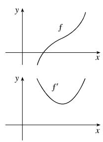
Instructor Manual: Stewart/Kokoska, Calculus: Concepts & Contexts Fifth Edition, Core 9780357632499; Chapter 2: Limits

Discuss what it means for to be positive, negative or zero. Then discuss what it means for to be increasing, decreasing or constant.

• Estimate derivatives from the graph of . Do this at various points, and plot the results on the blackboard. See if the class can recognize the graph as a graph of the cosine curve.
B. CLASS DISCUSSION
• Discuss properties of f ′ for

• Given the graph of below, have students determine where has a horizontal tangent, where is positive, where is negative, where is increasing (this may require some additional discussion), and where is decreasing. Then have them sketch the graph of .
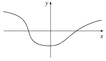
(For more exercises of this type using a wide variety of functions, use TEC Module 2.8.)
ANSWER There is a horizontal tangent near . is positive to the right of 0, negative to the left. is increasing between the -intercepts, and decreasing outside of them.
Instructor Manual: Stewart/Kokoska, Calculus: Concepts & Contexts Fifth Edition, Core 9780357632499; Chapter 2: Limits
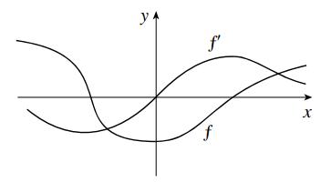
• TEC Module 2.8 can be used to develop students’ ability to look at the graph of a function and visualize the graph of that function’s derivative. The key feature of this module is that it allows the students to mark various features of the derivative directly on the graph of the function (for example, where the derivative is positive or negative). Then, after using this information and sketching a graph of the derivative, they can view the actual graph of the derivative and check their work
• Estimate the derivative of a function such as at various points, both numerically and by drawing an approximate tangent line at the blackboard and estimating the slope of that line. Use the estimates to attempt to construct a graph of the derivative of .


• Compute and if and . Point out that and discuss why the constant term is not important. Next, compute if . Point out that the graph of is just the graph of shifted up one unit, so the linear term just shifts derivatives. For more explorations on how the coefficients in polynomials and other functions affect first and second derivatives, use TEC Module 2.8.

• Consider the function . Show that it is not differentiable at 0 in two ways: by inspection (it has a cusp); and by computing the left- and right-hand

limits of at .
Instructor Manual: Stewart/Kokoska, Calculus: Concepts & Contexts Fifth Edition, Core 9780357632499; Chapter 2: Limits
Group Work 1: Tangent Lines and the Derivative Function
This simple exercise reinforces that although we are moving to thinking of the derivative as a function of x, it is still the slope of the line tangent to the graph of f
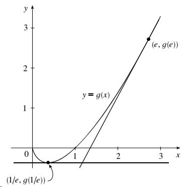

Group Work 2: The Revenge of Orville Redenbacher

In an advanced class, or a class in which one group has finished far ahead of the others, ask the students to repeat the exercise substituting “ , the density function” for . ANSWERS 1. 2.

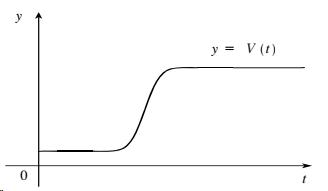
Instructor Manual: Stewart/Kokoska, Calculus: Concepts & Contexts Fifth Edition, Core 9780357632499; Chapter 2: Limits
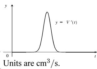
3.

Group Work 3: The Derivative Function

Give each group of between three and five students the picture of all eight graphs. They are to sketch the derivative functions by first estimating the slopes at points, and plotting the values of . Each group should also be given a large copy of one of the graphs, preferably on acetate. When they are ready, with this information they can draw the derivative graph on the same axes. For closure, look at all the graphs and their derivatives, pointing out salient features. Note that the derivative of graph 6 ( ) is itself. Also note that the derivative of graph 1 ( ) is not a straight line. Leave at least 15 minutes for closure. The whole exercise should take about 45–60 minutes, but it is really, truly worth the time.
If a group finishes early, have them discuss where is increasing and decreasing. Also show that where f is increasing, is positive, and where f is decreasing, is negative. For further exercises of this type, students can use TEC Module 2.8.
Instructor Manual: Stewart/Kokoska, Calculus: Concepts & Contexts Fifth Edition, Core 9780357632499; Chapter 2: Limits
ANSWERS
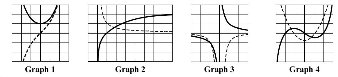

Group Work 4: Sorting Them Out
Students need to be comfortable with identifying salient features of the derivative functions before attempting this group work. It might take them some time to get used to the process involved. Version A is easier than Version B. If time is short, different groups can get different versions, as appropriate. If there is time, each group can be given both sheets.
ANSWERS
VERSION A


1. dashed, solid, gray
2. gray, solid, dashed
3. gray, dashed, solid
4. dashed, solid
VERSION B
1. dashed, solid, gray
2. solid, gray, dashed
3. solid, gray, dashed
4. dashed, solid
Instructor Manual: Stewart/Kokoska, Calculus: Concepts & Contexts Fifth Edition, Core 9780357632499; Chapter 2: Limits
BONUS PROBLEM
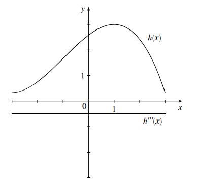
C. GROUP WORK ACTIVITY
GROUP WORK 1, SECTION 2.7 Tangent Lines and the Derivative Function
The following is a graph of .


It is a fact that the derivative of this function is .
1. Sketch the line tangent to at on the graph above.
2. Find an equation of the tangent line at .
3. Now sketch the line tangent to at


4. Find an equation of the tangent line at .
Instructor Manual: Stewart/Kokoska, Calculus: Concepts & Contexts Fifth Edition, Core 9780357632499; Chapter 2: Limits
Group Work 2: SECTION 2.7
The Revenge of Orville Redenbacher

1. Consider a single kernel of popcorn in a popcorn popper. Let be the volume in of the kernel at time t seconds. Draw a graph of , including as much detail as you can, up to the time that the kernel is taken from the popper.
2. Now sketch a graph of the derivative function . What are the units of ?

GROUP WORK 3, SECTION 2.7 The Derivative Function

3. Finally, sketch a graph of . What does it mean when ?
The graphs of several functions are shown below. For each function, estimate the slope of the graph of at various points. From your estimates, sketch graphs of .
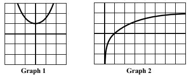

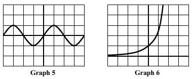
Instructor Manual: Stewart/Kokoska, Calculus: Concepts & Contexts Fifth Edition, Core 9780357632499; Chapter 2: Limits
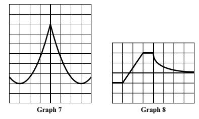
GROUP WORK 4, SECTION 2.7 Sorting Them Out (Version A)
Each figure below shows the graphs of a function , its first derivative, and its second derivative. Identify which is which.
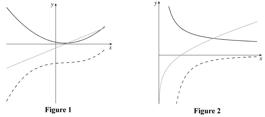
Instructor Manual: Stewart/Kokoska, Calculus: Concepts & Contexts Fifth Edition, Core 9780357632499; Chapter 2: Limits

Instructor Manual: Stewart/Kokoska, Calculus: Concepts & Contexts Fifth Edition, Core 9780357632499; Chapter 2: Limits
GROUP WORK 4, SECTION 2.7 Sorting Them Out (Version B)
Each figure below shows the graphs of a function g, its first derivative, and its second derivative. Identify which is which.


Instructor Manual: Stewart/Kokoska, Calculus: Concepts & Contexts Fifth Edition, Core 9780357632499; Chapter 2: Limits
GROUP WORK 4, SECTION 2.7 Sorting Them Out (Bonus Problem)
Given the following graph of , sketch a graph of


D. KNOWLEDGE CHECK
• If , what are the left- and right-hand limits obtained when trying to compute at ?

• Consider the graph of . Is this function defined at ? Continuous at ? Differentiable at ? Why
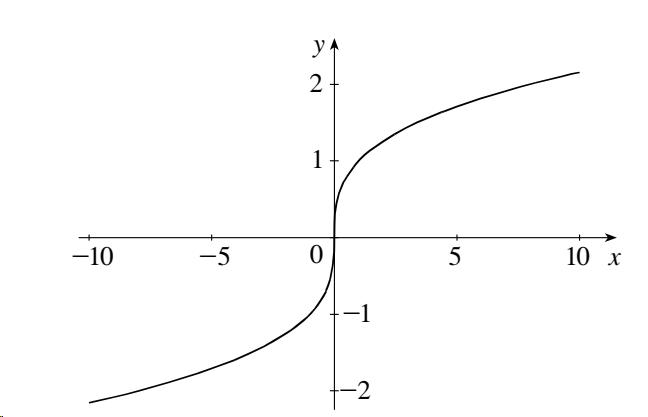
ANSWER It is defined and continuous, but not differentiable because it has a vertical tangent.
Instructor Manual: Stewart/Kokoska, Calculus: Concepts & Contexts Fifth Edition, Core 9780357632499; Chapter 2: Limits
E. HOMEWORK ASSIGNMENT
CORE EXERCISES 2, 3, 7, 12, 18, 54
SAMPLE ASSIGNMENT 1, 2, 3, 7, 8, 11, 12, 18, 20, 23, 27, 36, 39, 46, 53, 54, 66
Instructor Manual: Stewart/Kokoska, Calculus: Concepts & Contexts Fifth Edition, Core 9780357632499; Chapter 2: Limits
ADDITIONAL ACTIVITIES AND ASSIGNMENTS
WRITING PROJECT: Early Methods for Finding Tangents
The history of calculus is a fascinating and too-often neglected subject. Most people who study history never see calculus, and vice versa. We recommend assigning this section as extra credit to any motivated class, and possibly as a required group project, especially for a class consisting of students who are not science or math majors.
The students will need clear instructions detailing what their final result should look like. We recommend a page or two about Fermat’s or Barrow’s life and career, followed by two or three technical pages describing the alternate method of finding tangent lines as in the project’s directions, and completed by a final page or half page of meaningful conclusion.
Instructor Manual: Stewart/Kokoska, Calculus: Concepts & Contexts Fifth Edition, Core 9780357632499; Chapter 2: Limits
SAMPLE EXAM QUESTIONS
Problems marked with an asterisk (*) are particularly challenging and should be given careful consideration.
1. Consider the following graph of .
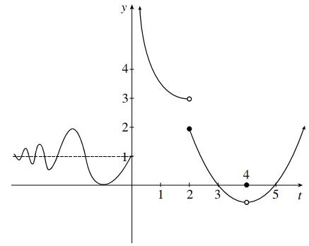


(a) What is ? ? ? ?
(b) For what values of x does exist?
(c) Does have any vertical asymptotes? If so, where?
(d) Does have any horizontal asymptotes? If so, where?
(e) For what values of is discontinuous?
2. Find values for and that will make continuous everywhere, if

3. Find the vertical and horizontal asymptotes for , where is a positive number.
4. Consider the function .

(a) What is the domain of ?
(b) Compute , if this limit exists.


(c) Is continuous at ? Explain your answer by either proving that is continuous at or telling how to modify to make it continuous.
Instructor Manual: Stewart/Kokoska, Calculus: Concepts & Contexts Fifth Edition, Core 9780357632499; Chapter 2: Limits

5. Let be a continuous function such that and . Classify the following statements as
A. Always true
B. Never true
C. Sometimes true
Justify your answers.
(a) (b) For some with (c) For all with (d) Given any in , then for some in (e) If or , then or . (f) for and for


6. Let be the function whose graph is given below.

(a) Sketch a plausible graph of .


(b) Sketch a plausible graph of a function such that and

Instructor Manual: Stewart/Kokoska, Calculus: Concepts & Contexts Fifth Edition, Core 9780357632499; Chapter 2: Limits

7. Suppose that the line tangent to the graph of at passes through the points and . (a) Find . (b) Find . (c) Find an equation of the line tangent to at .


8. Give examples of functions and with , and (a) (b) (c)

(d) Is it possible to have ? Either give an example or explain why it is not possible.
9. Each of the following limits represent the derivative of a function at some point . State a formula for and the value of the point . (a) (b) (c) (d)


Instructor Manual: Stewart/Kokoska, Calculus: Concepts & Contexts Fifth Edition, Core 9780357632499; Chapter 2: Limits
10. Let

(a) Evaluate each limit, if it exists. (i) (ii) (iii) (iv) (v) (vi) (vii) (viii)


(b) Where is discontinuous?
11.The graph of is given below. For which value(s) of is not differentiable? Justify your answer(s).
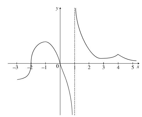
Instructor Manual: Stewart/Kokoska, Calculus: Concepts & Contexts Fifth Edition, Core 9780357632499; Chapter 2: Limits
12. A bicycle starts from rest and its distance travelled is recorded in the following table at one-second intervals.


(b) Estimate the speed after 2 seconds.
(c) Estimate the speed after 5 seconds.
(d) Estimate the speed after 6 seconds.
(e) Can we determine if the cyclist’s speed is constantly increasing? Explain.
(a) Compute the average speed of the bicycle from to and from to
13. Referring to the graphs given below, find each limit, if it exists. If a limit does not exist, explain why not.
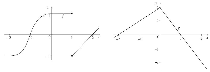
(a) (b) (c) (d) (e) (f) (g)


Instructor Manual: Stewart/Kokoska, Calculus: Concepts & Contexts Fifth Edition, Core 9780357632499; Chapter 2: Limits
14. The following is a graph of , the derivative of some function
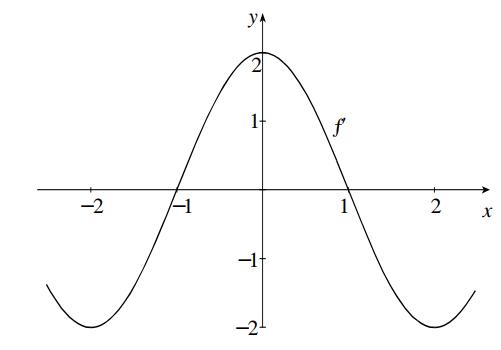
(a) Where is increasing?
(b) Where does have a local minimum? Where does have a local maximum?
(c) Where is concave up?
(d) Assuming that , sketch a possible graph of .
Instructor Manual: Stewart/Kokoska, Calculus: Concepts & Contexts Fifth Edition, Core 9780357632499; Chapter 2: Limits
Sample Exam Solutions


1. (a) , , , (b) exists for all x except and .
(c) There is a vertical asymptote at . (d) There is a horizontal asymptote at . (e) f is discontinuous at and 4.

2. Solve and to get


3. Taking gives a horizontal asymptote at . Algebraic simplification gives a vertical asymptote at . The function is undefined at , but there is no asymptote there because .
4.


(a) The domain is all values of except and (b) Algebraic simplification gives a limit of . (c) f is not continuous at , for it is not defined there. It can be modified by defining to be

5.
(a) C. True for , untrue for . (b) A. True by the Intermediate Value Theorem (c) C. True for , untrue for . (d) A. True by the Intermediate Value Theorem (e) C. True for , untrue for . (f) B. does not exist, contradicting the continuity of
6. (a) Answers will vary. Look for:
(i) zeros at 1 and 2


(ii) positive for ) and (2, 4) (iii) negative for (iv) flattens out for . (b) Answers will vary. Look for (i)
(ii) is always increasing (iii) is never perfectly flat (iv) is closest to being flat at (v) is concave up for and (vi) is concave down for
Instructor Manual: Stewart/Kokoska, Calculus: Concepts & Contexts Fifth Edition, Core 9780357632499; Chapter 2: Limits
7. (a)


(b) The equation of the tangent line is , so .

(c) The equation of the tangent line is .
8. Answers will vary; the following are samples only. (a) (b) (c)

(d) This is not possible. For , either or would have to be negative for large . This contradicts the assumption that .


9. Answers will vary (a) (b) (c) (d)


10. (a) (i) (ii) 1 (iii) Does not exist (iv) 9 (v) 9 (vi) 9 (vii) 3 (viii) 3 (b) is discontinuous at .

11. f isn’t differentiable at , because it is not continuous there; at , because it has a vertical tangent there; and at , because it has a cusp there.
12.
(a) Answers will vary. One good answer would be to compute the average speed between 1 and 2 (14 ft/s) and the average speed between 2 and 3 (18 ft/s) and average them to get 16 ft/s. This is also the answer obtained by computing the average speed between 1 and 3.
Instructor Manual: Stewart/Kokoska, Calculus: Concepts & Contexts Fifth Edition, Core 9780357632499; Chapter 2: Limits
(b) Answers will vary. Using reasoning similar to the previous part, we get an estimate of 22 ft/s, but it could be argued that a number closer to 22.5 would be more accurate.

(c) Answers will vary. The average speed between and is 22.5 ft/s.
(d) Since we are given information only about the cyclist’s position at one-second intervals, we cannot determine if the speed is constantly increasing. 13.
(a) (b) 0


(c) Does not exist, because while . (d)
(e) 1
(f) 2
(g) 0 14.

(a) is increasing on .
(b) Local minimum at ; local maximum at . (c) is concave up where is increasing, that is, on (d)