PDF Solutions Manual for Finite Mathematics 8th Edition by Waner

Finite Mathematics Solutions

Finite Mathematics Solutions

EIGHTH

EDITION

Stefan Waner Hofstra University

Steven R. Costenoble Hofstra University

Finite Mathematics Solutions, Eighth Edition

Stefan Waner, Steven R. Costenoble

SVP, Product: Erin Joyner

VP, Product: Thais Alencar

Portfolio Product Director: Mark Santee

Portfolio Product Manager: Jay Campbell

Product Assistant: Amelia Padilla

Learning Designer: Susan Pashos

Content Manager: Shelby Blakey

Digital Project Manager: John Smigielski

Product Marketing Manager: Taylor Shenberger

Content Acquisition Analyst: Nichole Nalenz

Production Service: Lumina Datamatics Ltd.

Designer: Gaby McCracken

Cover Image Source: Getty Images

© 2023, © 2018, © 2014 Cengage Learning, Inc.

Copyright © 2024 Cengage Learning, Inc. ALL RIGHTS RESERVED.

WCN: 02-300

No part of this work covered by the copyright herein may be reproduced or distributed in any form or by any means, except as permitted by U.S. copyright law, without the prior written permission of the copyright owner.

Unless otherwise noted, all content is Copyright © Cengage Learning, Inc.

For product information and technology assistance, contact us at Cengage Customer & Sales Support, 1-800-354-9706 or support.cengage.com.

For permission to use material from this text or product, submit all requests online at www.copyright.com.

Library of Congress Control Number: 2023936216

Student Edition:

ISBN: 978-0-357-72326-5

Loose-leaf Edition:

ISBN: 978-0-357-72327-2

Cengage

5191 Natorp Boulevard Mason, OH 45040 USA

Cengage is a leading provider of customized learning solutions. Our employees reside in nearly 40 different countries and serve digital learners in 165 countries around the world. Find your local representative at www.cengage.com.

To learn more about Cengage platforms and services, register or access your online learning solution, or purchase materials for your course, visit www.cengage.com.

Printed in the United States of America Print Number: 01 Print Year: 2024

CHAPTER 4 Matrix Algebra 262

4.1 Solutions Section 262

4.2 Solutions Section 272

4.3 Solutions Section 288

4.4 Solutions Section 308

4.5 Solutions Section 329

SOLUTIONS CHAPTER 4 REVIEW 340

CASE STUDY Solutions Chapter 4 352

CHAPTER 5 Linear Programming

5.1 Solutions Section 353

5.2 Solutions Section 372

5.3 Solutions Section 395

5.4 Solutions Section 445

5.5 Solutions Section 503

SOLUTIONS CHAPTER 5 REVIEW 536

CASE STUDY Solutions Chapter 5 567

CHAPTER 6 Sets and Counting

6.1 Solutions Section 568

6.2 Solutions Section 580

6.3 Solutions Section 592

6.4 Solutions Section 601

SOLUTIONS CHAPTER 6 REVIEW 613

CASE STUDY Solutions Chapter 6 621

CHAPTER 7 Probability

7.1 Solutions Section 622

7.2 Solutions Section 633

7.3 Solutions Section 643

7.4 Solutions Section 656

7.5 Solutions Section 664

7.6 Solutions Section 683

7.7 Solutions Section 692

SOLUTIONS CHAPTER 7 REVIEW 708

CASE STUDY Solutions Chapter 7 718

568

622

CHAPTER 8 Random Variables and Statistics 720

8.1 Solutions Section 720

8.2 Solutions Section 733

8.3 Solutions Section 744

8.4 Solutions Section 759

8.5 Solutions Section 777

SOLUTIONS CHAPTER 8 REVIEW 788

CASE STUDY Solutions Chapter 8 801

Chapter 0 Precalculus Review

Solutions Section 0.1

Section 0.1

1. 2(4 + ( 1))(2 4) = 2(3)( 8) = (6)( 8) = 48

3. 20∕(3 * 4) 1 = 20 12 1 = 5 3 1 = 2 3

2. 3 + ([4 2] 9) = 3 + (2 × 9) = 3 + 18 = 21

4. 2 (3 * 4)∕10 = 2 12 10 = 2 6 5 = 4 5

5. 3 + ([3 + ( 5)]) 3 2 × 2 = 3 + ( 2) 3 4 = 1 1 = 1 6. 12 (1 4) 2(5 1) ⋅ 2 1 = 12 ( 3) 16 1 = 15 15 = 1

7. (2 5 * ( 1))∕1 2 * ( 1) = 2 5 ⋅ ( 1) 1 2 ⋅ ( 1) = 2 + 5 1 + 2 = 7 + 2 = 9

8. 2 5 * ( 1)∕(1 2 * ( 1)) = 2 5 ⋅ ( 1) 1 2 ( 1) = 2 5 1 + 2 + 2 = 2 + 5 3 = 11 5

9. 2 ⋅ ( 1) 2∕2 = 2 × ( 1) 2 2 = 2 × 1 2 = 2 2 = 1 10. 2 + 4 ⋅ 3 2 = 2 + 4 × 9 = 2 + 36 = 38

11. 2 ⋅ 4 2 + 1 = 2 × 16 + 1 = 32 + 1 = 33 12. 1 3 ⋅ ( 2) 2 × 2 = 1 3 × 4 × 2 = 1 24 = 23

13. 3^2+2^2+1 = 3 2 + 2 2 + 1 = 9 + 4 + 1 = 14 14. 2^(2^2-2) = 2 (2 2 2) = 2 4 2 = 2 2 = 4

15. 3 2( 3) 2 6(4 1) 2 = 3 2 × 9 6(3) 2 = 3 18 6 × 9 = 15 54 = 5 18 16. 1 2(1 4) 2 2(5 1) 2 2 = 1 2( 3) 2 2(4) 2 2 = 1 2 × 9 2 × 16 × 2 = 1 18 64 = 17 64

17. 10*(1+1/10)^3 = 10(1 + 1 10 ) 3 = 10(1 1) 3 = 10 × 1 331 = 13 31 18. 121/(1+1/10)^2 = 121 !1 + 1 10 " 2 = 121 1.1 2 = 121 1.21 = 100

19. 3[ 2 ⋅ 3 2 (4 1) 2 ] = 3⎡ ⎣ ⎢ ⎢ 2 × 9 3 2 ⎤ ⎦ ⎥ ⎥ = 3[ 18 9 ] = 3 × 2 = 6 20. [ 8(1 4) 2 9(5 1) 2 ] = [ 8 × 9 9 × 16 ] = ( 72 144 ) = ( 1 2 ) = 1 2

21. 3⎡ ⎣ ⎢ ⎢1 ( 1 2 ) 2⎤ ⎦ ⎥ ⎥ 2 + 1 = 3[1 1 4 ] 2 + 1 = 3[ 3 4 ] 2 + 1 = 3[ 9 16 ] + 1 = 27 16 + 1 = 43 16 22. 3⎡ ⎣ ⎢ ⎢ 1 9 ( 2 3 ) 2⎤ ⎦ ⎥ ⎥ 2 + 1 = 3[ 1 9 4 9 ] 2 + 1 = 3[ 3 9 ] 2 + 1 = 3[ 1 3 ] 2 + 1 = 3 1 9 + 1 = 3 9 + 1 = 4 3

23. (1/2)^2-1/2^2 = # 1 2 $ 2 1 2 2 = 1 4 1 4 = 0 24. 2/(1^2)-(2/1)^2 = 2 1 2 # 2 1 $ 2 = 2 1 4 1 = 2

25. 3 × (2 5) = 3*(2-5) 26. 4 + 5 9 = 4+5/9 or 4+(5/9)

27. 3 2 5 = 3/(2-5) 28. 4 1 3 = (4-1)/3

29. 3 1 8 + 6 = (3-1)/(8+6)

Note 3-1/8-6 is wrong, as it corresponds to 3 1 8 6 30. 3 + 3 2 9 = 3+3/(2-9)

31. 3 4 + 7 8 = 3-(4+7)/8 32. 4 × 2 ! 2 3 " = 4*2/(2/3) or (4*2)/(2/3)

33. 2 3 + 𝑥 𝑥𝑦 2 = 2/(3+x)-x*y^2 34. 3 + 3 + 𝑥 𝑥𝑦 = 3+(3+x)/(x*y)

35. 3.1𝑥 3 4𝑥 2 60 𝑥 2 1 = 3.1x^3-4x^(-2)-60/(x^2-1) 36. 2 1𝑥 3 𝑥 1 + 𝑥 2 3 2 = 2.1x^(-3)-x^(-1)+(x^2-3)/2

37. ! 2 3 " 5 = (2/3)/5 38. 2 ! 3 5 " = 2/(3/5)

39. 3 4 5 × 6 = 3^(4-5)*6

Note that the entire exponent is in parentheses.

40. 2 3+5 7 9 = 2/(3+5^(7-9))

Note that the entire exponent is in parentheses.

41. 3(1 + 4 100 ) 3 = 3*(1+4/100)^(-3) 42. 3( 1 + 4 100 ) 3 = 3((1+4)/100)^(-3)

43. 3 2𝑥 1 + 4 𝑥 1 = 3^(2*x-1)+4^x-1 44. 2 𝑥 2 (2 2𝑥) 2 = 2^(x^2)-(2^(2*x))^2

45. 2 2𝑥 2 𝑥+1 = 2^(2x^2-x+1)

Note that the entire exponent is in parentheses.

47. 4𝑒 2𝑥 2 3

= 4*e^(-2*x)/(2-3e^(-2*x)) or 4(*e^(-2*x))/(2-3e^(-2*x)) or (4*e^(-2*x))/(2-3e^(-2*x))

Note that the entire exponent is in parentheses.

= (e^(2*x)+e^(-2*x))/(e^(2*x)e^(-2*x))

49. 3(1 ! 1 2 " 2) 2 + 1 = 3(1-(-1/2)^2)^2+1 50. 3⎛ ⎝ ⎜ ⎜ 1 9 ( 2 3 ) 2⎞ ⎠ ⎟ ⎟ 2 + 1 = 3(1/9-(2/3)^2)^2+1

Section 0.2

53. 𝑥 2 (1 + 2𝑥) 2 = 0 ⇒ 𝑥 2 = (1 + 2𝑥)

If 𝑥 = 1 + 2𝑥, then 𝑥 = 1 ⇒ 𝑥 = 1. If 𝑥 = (1 + 2𝑥), then = 1 ⇒ 𝑥 = 1 3 .

So, 𝑥 = 1 or 1 3

23. (𝑥 + 1)(𝑥 + 2) + (𝑥 + 1)(𝑥 + 3)

= (𝑥 + 1)(𝑥 + 2 + 𝑥 + 3)

= (𝑥 + 1)(2𝑥 + 5)

25. (𝑥 2 + 1) 5(𝑥 + 3) 4 + (𝑥 2 + 1) 6(𝑥 + 3) 3 = (𝑥 2 + 1) 5(𝑥 + 3) 3(𝑥 + 3 + 𝑥 2 + 1)

24. (𝑥 + 1)(𝑥 + 2) 2 + (𝑥 + 1) 2(𝑥 + 2)

= (𝑥 + 1)(𝑥 + 2)(𝑥 + 2 + 𝑥 + 1)

= (𝑥 + 1)(𝑥 + 2)(2𝑥 + 3)

= (𝑥 2 + 1) 5(𝑥 + 3) 3(𝑥 2 + 𝑥 + 4) 26. 10𝑥(𝑥 2 + 1) 4(𝑥 3 + 1) 5 + 15𝑥 2(𝑥 2 + 1) 5(𝑥 3 + 1) 4 = 5𝑥(𝑥 2 + 1) 4(𝑥 3 + 1) 4[2(𝑥 3 + 1) + 3𝑥(𝑥 2 + 1)] = 5𝑥(𝑥 2 + 1) 4(𝑥 3 + 1) 4(5𝑥 3 + 3𝑥 + 2)

27. (𝑥 3 + 1) 𝑥 + 1 √ (𝑥 3 + 1) 2 𝑥 + 1 √ = (𝑥 3 + 1) 𝑥 + 1 √ ⋅ [1 (𝑥 3 + 1)]

𝑥 3(𝑥 3 + 1) 𝑥 + 1 √ 28. (𝑥 2 + 1) 𝑥 + 1 √ (𝑥 + 1) 3 √ = 𝑥 + 1 √ ⋅ [𝑥 2 + 1 (𝑥 + 1) 2 √ ] = 𝑥 + 1 √ ⋅ [𝑥 2 + 1 (𝑥 + 1)] = (𝑥 2 𝑥) 𝑥 + 1 √ = 𝑥(𝑥 1) 𝑥 + 1 √

29. (𝑥 + 1) 3 √ + (𝑥 + 1) 5 √ = (𝑥 + 1) 3 √ ⋅ [1 + (𝑥 + 1) 2 √ ] = (𝑥 + 1) 3 √ ⋅ (1 + 𝑥 + 1) = (𝑥 + 2) (𝑥 + 1) 3 √ 30. (𝑥 2 + 1) (𝑥 + 1) 4 3 √ (𝑥 + 1) 7 3 √ = (𝑥 + 1) 4 3 √ [𝑥 2 + 1 (𝑥 + 1) 3 3 √ ] = (𝑥 + 1) 4 3 √ [𝑥 2 + 1 (𝑥 + 1)] = (𝑥 2 𝑥) (𝑥 + 1) 4 3 √ = 𝑥(𝑥 1) (𝑥 + 1) 4 3 √

31. 𝑎 = 2, 𝑏 = 6, 𝑐 = 5, so that the discriminant is 𝑏 2 4𝑎𝑐 = 6 2 4(2)(5) = 36 40 = 4

As the discriminant is negative, the expression does not factor at all.

32. 𝑎 = 4, 𝑏 = 6, 𝑐 = 2, so that the discriminant is 𝑏 2 4𝑎𝑐 = ( 6) 2 4(4)(2) = 36 32 = 4 = 2 2

As the discriminant is a perfect square, the expression factors over the integers.

33. 𝑎 = 3, 𝑏 = 2, 𝑐 = 3, so that the discriminant is 𝑏 2 4𝑎𝑐 = ( 2) 2 4( 3)(3) = 4 + 36 = 40

As the discriminant is positive but not a perfect square, the expression factors, but not over the integers.

34. 𝑎 = 1, 𝑏 = 4, 𝑐 = 7, so that the discriminant is 𝑏 2 4𝑎𝑐 = ( 4) 2 4(1)( 7) = 16 + 28 = 44

As the discriminant is positive but not a perfect square, the expression factors, but not over the integers.

35. 𝑎 = 8, 𝑏 = 12, 𝑐 = 4, so that the discriminant is 𝑏 2 4𝑎𝑐 = 12 2 4(8)(4) = 144 128 = 16 = 4 2

As the discriminant is a perfect square, the expression factors over the integers.

36. 𝑎 = 1, 𝑏 = 2, 𝑐 = 19, so that the discriminant is 𝑏 2 4𝑎𝑐 = 2 2 4(1)(19) = 4 76 = 72

As the discriminant is negative, the expression does not factor at all.

37. 𝑎 = 40, 𝑏 = 64, 𝑐 = 24, so that the discriminant is 𝑏 2 4𝑎𝑐 = ( 64) 2 4(40)(24) = 4,096 3,840 = 256 = 16 2

As the discriminant is a perfect square, the expression factors over the integers.

38. 𝑎 = 10, 𝑏 = 32, 𝑐 = 32, so that the discriminant is 𝑏 2 4𝑎𝑐 = ( 32) 2 4( 10)( 32) = 1,024 1,280 = 256

As the discriminant is negative, the expression does not factor at all.

39. 𝑎 = 6, 𝑏 = 22, 𝑐 = 16, so that the discriminant is 𝑏 2 4𝑎𝑐 = ( 22) 2 4(6)(16) = 484 384 = 100 = 10 2

As the discriminant is a perfect square, the expression factors over the integers.

40. 𝑎 = 48, 𝑏 = 32, 𝑐 = 4, so that the discriminant is 𝑏 2 4𝑎𝑐 = 32 2 4(48)(4) = 1,024 768 = 256 = 16 2

As the discriminant is a perfect square, the expression factors over the integers.

41. a. 2𝑥 + 3𝑥 2 = 𝑥(2 + 3𝑥)

b. 𝑥(2 + 3𝑥) = 0

𝑥 = 0 or 2 + 3𝑥 = 0

𝑥 = 0 or 2∕3

43. a. 6𝑥 3 2𝑥 2 = 2𝑥 2(3𝑥 1)

b. 2𝑥 2(3𝑥 1) = 0

𝑥 2 = 0 or 3𝑥 1 = 0

𝑥 = 0 or 1∕3

45. a. 𝑥 2 8𝑥 + 7 = (𝑥 1)(𝑥 7)

b. (𝑥 1)(𝑥 7) = 0

𝑥 1 = 0 or 𝑥 7 = 0

𝑥 = 1 or 7

47. a. 𝑥 2 + 𝑥 12 = (𝑥 3)(𝑥 + 4)

b. (𝑥 3)(𝑥 + 4) = 0

𝑥 3 = 0 or 𝑥 + 4 = 0

𝑥 = 3 or 4

49. a. 2𝑥 2 3𝑥 2 = (2𝑥 + 1)(𝑥 2)

b. (2𝑥 + 1)(𝑥 2) = 0

2𝑥 + 1 = 0 or 𝑥 2 = 0

𝑥 = 1∕2 or 2

42. a. 𝑦 2 4𝑦 = 𝑦(𝑦 4) b. 𝑦(𝑦 4) = 0

𝑦 = 0 or 𝑦 4 = 0 𝑦 = 0 or 4

44. a. 3𝑦 3 9𝑦 2 = 3𝑦 2(𝑦 3)

b. 3𝑦 2(𝑦 3) = 0

𝑦 2 = 0 or 𝑦 3 = 0 𝑦 = 0 or 3

46. a. 𝑦 2 + 6𝑦 + 8 = (𝑦 + 2)(𝑦 + 4)

b. (𝑦 + 2)(𝑦 + 4) = 0

𝑦 + 2 = 0 or 𝑦 + 4 = 0

𝑦 = 2 or 4

48. a. 𝑦 2 + 𝑦 6 = (𝑦 2)(𝑦 + 3)

b. (𝑦 2)(𝑦 + 3) = 0

𝑦 2 = 0 or 𝑦 + 3 = 0

𝑦 = 2 or 3

50. a. 3𝑦 2 8𝑦 3 = (3𝑦 + 1)(𝑦 3)

b. (3𝑦 + 1)(𝑦 3) = 0

3𝑦 + 1 = 0 or 𝑦 3 = 0

𝑦 = 1∕3 or 3

51. a. 6𝑥 2 + 13𝑥 + 6 = (2𝑥 + 3)(3𝑥 + 2)

b. (2𝑥 + 3)(3𝑥 + 2) = 0

2𝑥 + 3 = 0 or 3𝑥 + 2 = 0

𝑥 = 3∕2 or 2∕3

53. a. 12𝑥 2 + 𝑥 6 = (3𝑥 2)(4𝑥 + 3)

b. (3𝑥 2)(4𝑥 + 3) = 0

3𝑥 2 = 0 or 4𝑥 + 3 = 0

𝑥 = 2∕3 or 3∕4

55. a. 𝑥 2 + 4𝑥𝑦 + 4𝑦 2 = (𝑥 + 2𝑦) 2

b. (𝑥 + 2𝑦) 2 = 0

𝑥 + 2𝑦 = 0

𝑥 = 2𝑦

57. a. 𝑥 4 5𝑥 2 + 4 = (𝑥 2 1)(𝑥 2 4) = (𝑥 + 1)(𝑥 1)(𝑥 + 2)(𝑥 2)

b. (𝑥 + 1)(𝑥 1)(𝑥 + 2)(𝑥 2) = 0

𝑥 + 1 = 0 or 𝑥 1 = 0 or 𝑥 + 2 = 0 or 𝑥 2 = 0

𝑥 = ±1 or ±2

59. a. 𝑥 2 3 = (𝑥 3√ )(𝑥 + 3√ )

b. (𝑥 3√ )(𝑥 + 3√ ) = 0

𝑥 3√ = 0 or 𝑥 + 3√ = 0

𝑥 = ± 3√

52. a. 6𝑦 2 + 17𝑦 + 12 = (3𝑦 + 4)(2𝑦 + 3)

b. (3𝑦 + 4)(2𝑦 + 3) = 0 3𝑦 + 4 = 0 or 2𝑦 + 3 = 0

𝑦 = 4∕3 or 3∕2

54. a. 20𝑦 2 + 7𝑦 3 = (4𝑦 1)(5𝑦 + 3)

b. (4𝑦 1)(5𝑦 + 3) = 0 4𝑦 1 = 0 or 5𝑦 + 3 = 0 𝑦 = 1∕4 or 3∕5

56. a. 4𝑦 2 4𝑥𝑦 + 𝑥 2 = (2𝑦 𝑥) 2 b. (2𝑦 𝑥) 2 = 0 2𝑦 𝑥 = 0 𝑦 = 𝑥∕2

58. a. 𝑦 4 + 2𝑦 2 3 = (𝑦 2 1)(𝑦 2 + 3) = (𝑦 + 1)(𝑦 1)(𝑦 2 + 3)

b. (𝑦 + 1)(𝑦 1)(𝑦 2 + 3) = 0

𝑦 + 1 = 0 or 𝑦 1 = 0 or 𝑦 2 + 3 = 0

𝑦 = ±1 (Notice that 𝑦 2 + 3 = 0 has no real solutions.)

60. a. 𝑦 2 7 = (𝑦 7√ )(𝑦 + 7√ )

b. (𝑦 7√ )(𝑦 + 7√ ) = 0

𝑦 7√ = 0 or 𝑦 + 7√ = 0

𝑦 = ± 7√

Section 0.5

+ 1) 3(𝑥 + 2) 2 (𝑥 + 2) 6 = (𝑥 + 1) 2(𝑥 + 2) 2[(𝑥 + 2) (𝑥 + 1)] (𝑥 + 2) 6 = (𝑥 + 1) 2 (𝑥 + 2) 4 12. 6𝑥(𝑥 2 + 1) 2(𝑥 3 + 2) 3 9𝑥 2(𝑥 2 + 1) 3(𝑥 3 + 2)

Section 0.7

1.

∕2

6. (𝑥 + 1)(𝑥 + 2) 2 + (𝑥 + 1) 2(𝑥 + 2) = 0, (𝑥 + 1)(𝑥 + 2)(𝑥 + 2 + 𝑥 + 1) = 0, (𝑥 + 1)(𝑥 + 2)(2𝑥 + 3) = 0, 𝑥 = 1, 2, 3∕2

7. (𝑥 2 + 1) 5(𝑥 + 3) 4 + (𝑥 2 + 1) 6(𝑥 + 3) 3 = 0, (𝑥 2 + 1) 5(𝑥 + 3) 3(𝑥 + 3 + 𝑥 2 + 1) = 0, (𝑥 2 + 1) 5(𝑥 + 3) 3(𝑥 2 + 𝑥 + 4) = 0, 𝑥 = 3 (Neither 𝑥 2 + 1 = 0 nor 𝑥 2 + 𝑥 + 4 = 0 has a real solution.)

8. 10𝑥(𝑥 2 + 1) 4(𝑥 3 + 1) 5 10𝑥 2(𝑥 2 + 1) 5(𝑥 3 + 1) 4 = 0, 10𝑥(𝑥 2 + 1) 4(𝑥 3 + 1) 4[𝑥 3 + 1 𝑥(𝑥 2 + 1)] = 0, 10𝑥(𝑥 2 + 1) 4(𝑥 3 + 1) 4(1 𝑥) = 0, 𝑥 = 1, 0, 1

9. (𝑥 3 + 1) 𝑥 + 1 √ (𝑥 3 + 1) 2 𝑥 + 1 √ = 0, (𝑥 3 + 1) 𝑥 + 1 √ [1 (𝑥 3 + 1)] = 0, 𝑥 3(𝑥 3 + 1) 𝑥 + 1 √ = 0, 𝑥 = 0, 1

10. (𝑥 2 + 1) 𝑥 + 1 √ (𝑥 + 1) 3 √ = 0, 𝑥 + 1 √ [𝑥 2 + 1 (𝑥 + 1)] = 0, (𝑥 2 𝑥) 𝑥 + 1 √ = 0, 𝑥(𝑥 1) 𝑥 + 1 √ = 0, 𝑥 = 1, 0, 1

11. (𝑥 + 1) 3 √ + (𝑥 + 1) 5 √ = 0, (𝑥 + 1) 3 √ (1 + 𝑥 + 1) = 0, (𝑥 + 2) (𝑥 + 1) 3 √ = 0, 𝑥 = 1 (𝑥 = 2 is not a solution because (𝑥 + 1) 3 √ is not defined for 𝑥 = 2 )

12. (𝑥 2 + 1) (𝑥 + 1) 4 3 √ (𝑥 + 1) 7 3 √ = 0, (𝑥 + 1) 4 3 √ [𝑥 2 + 1 (𝑥 + 1)] = 0, (𝑥 2 𝑥) (𝑥 + 1) 4 3 √ = 0, 𝑥(𝑥 1) (𝑥 + 1) 4 3 √ = 0, 𝑥 = 1, 0, 1

13. (𝑥 + 1) 2(2𝑥 + 3) (𝑥 + 1)(2𝑥 + 3) 2 = 0, (𝑥 + 1)(2𝑥 + 3)(𝑥 + 1 2𝑥 3) = 0, (𝑥 + 1)(2𝑥 + 3)( 𝑥 2) = 0, 𝑥 = 2, 3∕2, 1

14. (𝑥 2 1) 2(𝑥 + 2) 3 (𝑥 2 1) 3(𝑥 + 2) 2 = 0,

(𝑥 2 1) 2(𝑥 + 2) 2(𝑥 + 2 𝑥 2 + 1) = 0, (𝑥 2 1) 2(𝑥 + 2) 2(𝑥 2 𝑥 3) = 0, 𝑥 = 2, 1, 1, (1 ± 13√ )∕2

15. (𝑥 + 1) 2(𝑥 + 2) 3 (𝑥 + 1) 3(𝑥 + 2) 2 (𝑥 + 2) 6 = 0,

(𝑥 + 1) 2(𝑥 + 2) 2[(𝑥 + 2) (𝑥 + 1)] (𝑥 + 2) 6 = 0,

(𝑥 + 1) 2

(𝑥 + 2) 4 = 0, (𝑥 + 1) 2 = 0, 𝑥 = 1

16. 6𝑥(𝑥 2 + 1) 2(𝑥 2 + 2) 4 8𝑥(𝑥 2 + 1) 3(𝑥 2 + 2) 3 (𝑥 2 + 2) 8 = 0, 2𝑥(𝑥 2 + 1) 2(𝑥 2 + 2) 3[3(𝑥 2 + 2) 4(𝑥 2 + 1)] (𝑥 2 + 2) 8 = 0, 2𝑥(𝑥 2 + 1) 2(𝑥 2 2) (𝑥 2 + 2) 5 = 0,

2𝑥(𝑥 2 + 1) 2(𝑥 2 2) = 0, 𝑥 = 0, ± 2√

17. 2(

Section 0.8

Solutions Section 0.8

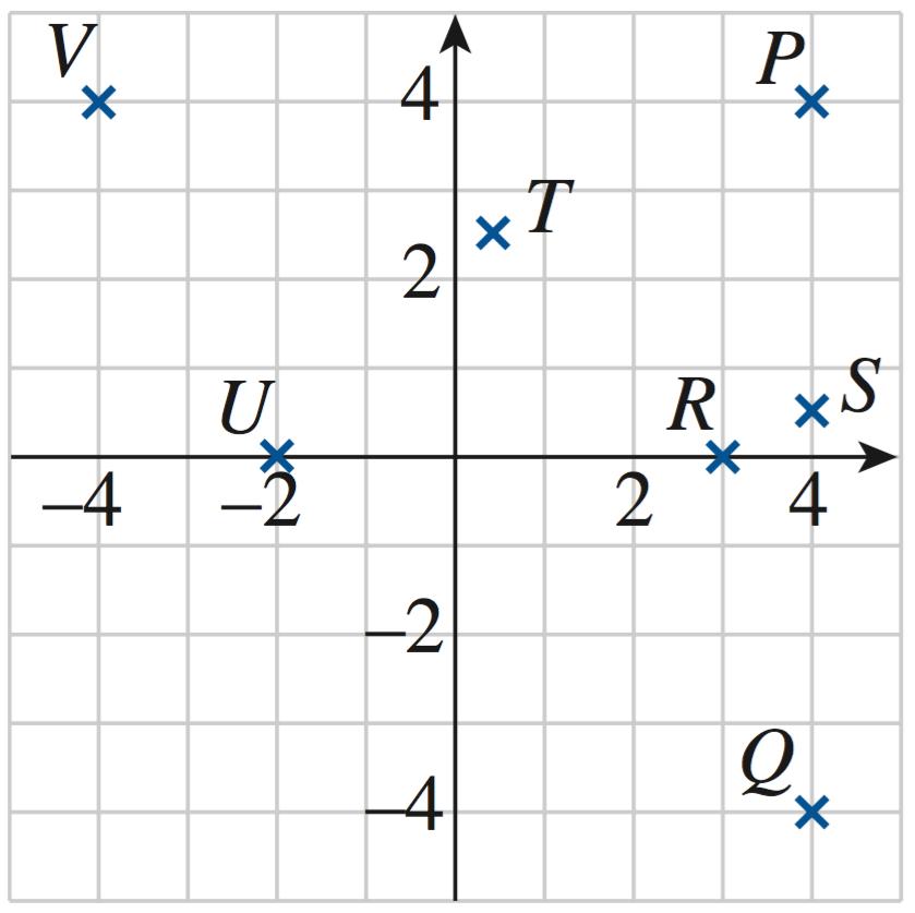
1. 𝑃 (0, 2), 𝑄(4, 2), 𝑅( 2, 3), 𝑆( 3 5, 1 5), 𝑇 ( 2 5, 0), 𝑈 (2, 2 5)

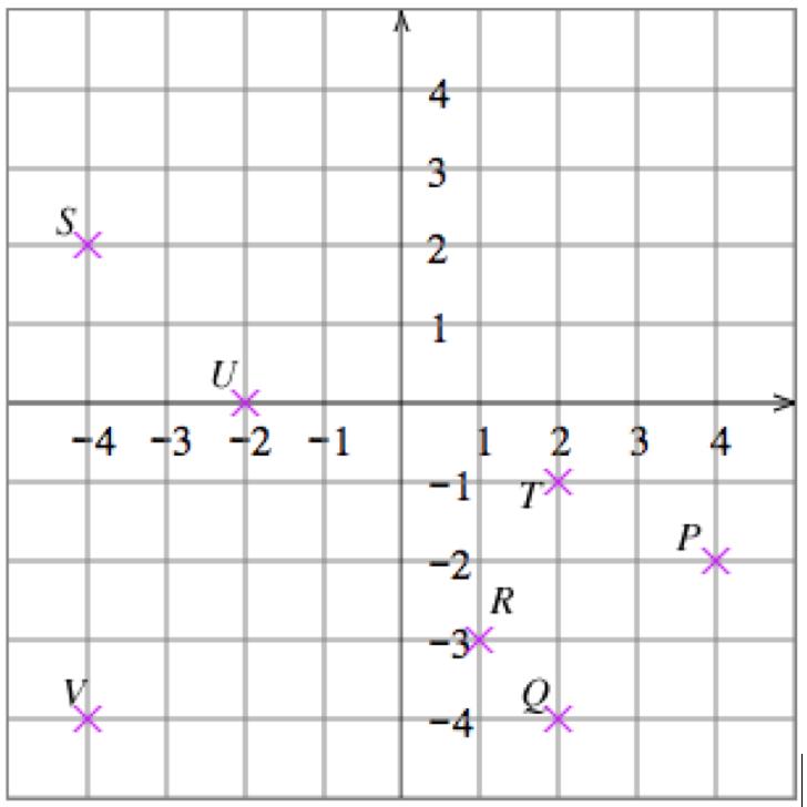
2. 𝑃 ( 2, 2), 𝑄(3 5, 2), 𝑅(0, 3), 𝑆( 3 5, 1 5), 𝑇 (2 5, 0), 𝑈 ( 2, 2 5) 3.

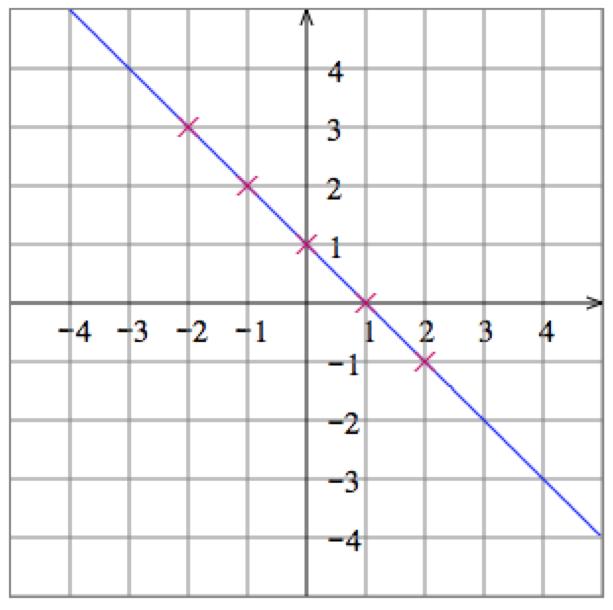
5. Solve the equation 𝑥 + 𝑦 = 1 for 𝑦 to get 𝑦 = 1 𝑥 Then plot some points:

Graph:

6. Solve the equation 𝑦 𝑥 = 1 for 𝑦 to get 𝑦 = 1 + 𝑥 Then plot some points:

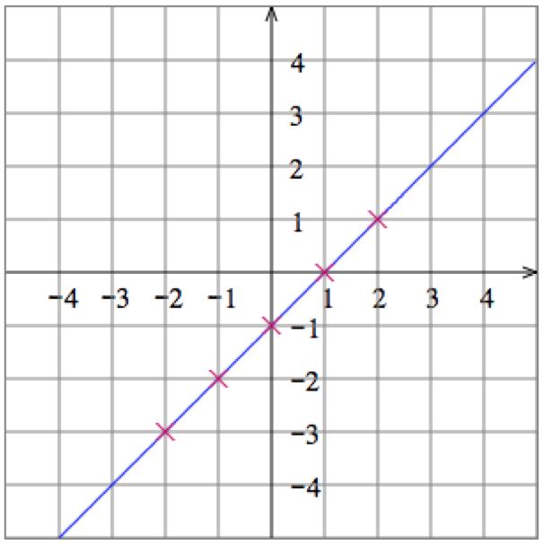
Graph:

9. Solve the equation 𝑥𝑦 = 4 for 𝑦 to get 𝑦 = 4

. Then plot some points:

Graph:

10. Solve the equation

12. Solve the equation

. Then plot some points: Graph:

17.

18. Set the two distances equal and solve:

19. Circle with center (0, 0) and radius 3

20. The single point (0, 0).

5. log4 16 = the power to which we need to raise 4 in order to get 16. Because 4 boxed 2 = 16, this power is 2, so log4 16 = 2.

6. log5 125 = the power to which we need to raise 5 in order to get

is 3, so log5 125 = 3.

7. log5 1 25 = the

log5 1 25 = 2 8. log4 1 64 = the power to which we

is 3, so log4 1 64 = 3.

Solutions Section 0.9

9. log 100,000 = log10 100,000 = the power to which we need to raise 10 in order to get 100,000 Because 10 boxed 5 = 100,000, this power is 5, so log 100,000 = 5

10. log 1,000 = log10 1,000 = the power to which we need to raise 10 in order to get 1,000. Because 10 boxed 3 = 1,000, this power is 3, so log 1,000 = 3

11. log16 16 = the power to which we need to raise 16 in order to get 16. Because 16 boxed 1 = 16, this power is 1, so log16 16 = 1.

12. log1∕2 1 2 = the power to which we need to raise 1 2 in order to get 1 2 . Because ! 1 2 " boxed 1 = 1 2 , this power is 1, so log1∕2 1 2 = 1

13. log4 1 16 = the power to which we need to raise 4 in order to get 1 16 Because 4 boxed 2 = 1 16 , this power is 2, so log4 1 16 = 2.

14. log2 1 8 = the power to which we need to raise 2 in order to get 1 8 Because 2 boxed 3 = 1 8 , this power is 3, so log2 1 8 = 3

15. log2 2√ = the power to which we need to raise 2 in order to get 2√ . Because 2 boxed 1∕2 = 2√ , this power is 1 2 , so log2 2√ = 1 2 .

16. log4 2√ = the power to which we need to raise 4 in order to get 2√ Because 4 boxed 1∕4 = 2√ , this power is 1 4 , so log4 2√ = 1 4

17. By Identity (1), log𝑏 3 + log𝑏 4 = log𝑏 (3 × 4) = log𝑏 boxed 12

18. By Identity (2), log𝑏 3 log𝑏 4 = log𝑏 boxed 3 4

19. log𝑏 2 log𝑏 5 log𝑏 4 = log𝑏 2 (log𝑏 5 + log𝑏 4) = log𝑏 2 (log𝑏 (5 × 4)) (Identity 1) = log𝑏 ! 2 5 × 4 " (Identity 2) = log𝑏 boxed 1 10

20. log𝑏 3 + log𝑏 2 log𝑏 7 = log𝑏 (3 × 2) log𝑏 7 (Identity 1) = log𝑏 ! 3 × 2 7 " (Identity 2) = log𝑏 boxed 6 7

21. log𝑏 3 3 log𝑏 2 = log𝑏 3 log𝑏 2 3 (Identity 3) = log𝑏 ! 3 2 3 " (Identity 2) = log𝑏 boxed 3 8

22. 3 log𝑏 2 + 2 log𝑏 3 = log𝑏 2 3 + log𝑏 3 2 (Identity 3) = log𝑏 (2 3 × 3 2) (Identity 1) = log𝑏 boxed 72

23. 4 log𝑏 𝑥 + 5 log𝑏 𝑦 = log𝑏 𝑥 4 + log𝑏 𝑦 5 (Identity 3) = log𝑏 boxed 𝑥 4 𝑦 5 (Identity 1)

24. 3

25.

26.

27. 𝑥 log𝑏 2 2 log𝑏 𝑥 = log𝑏 2 𝑥 log𝑏 𝑥 2 (Identity 3)

28. 𝑝 log𝑏 𝑞 + 𝑞 log𝑏 𝑝 = log𝑏

29. log 21 = log(3 × 7) = log 3 + log 7 = 𝑏 + 𝑐 (Identity 1)

30. log 14 = log(2 × 7) = log 2 + log 7 = 𝑎 + 𝑐 (Identity 1)

31. log 42 = log(2 × 3 × 7) = log 2 + log 3 + log 7 = 𝑎 + 𝑏 + 𝑐 (Identity 1)

32. log 28 = log(2 × 2 × 7) = log 2 + log 2 + log 7 = 2𝑎 + 𝑐 (Identity 1)

33. log! 1 7 " = log 7 = 𝑐 (Identity 5)

34. log! 1 3 " = log 3 = 𝑏 (Identity 5)

35. log! 2 3 " = log 2 log 3 = 𝑎 𝑏 (Identity 2)

36. log! 7 2 " = log 7 log 2 = 𝑐 𝑎 (Identity 2)

37. log! 4 7 " = log 4 log 7 (Identity 2) = log 2 + log 2 log 7 (Identity 1) = 2𝑎 𝑐

38. log! 2 9 " = log 2 log 9 (Identity 2) = log 2 (log 3 + log 3) (Identity 1) = 𝑎 2𝑏

39. log 16 = log 2 4 = 4 log 2 = 4𝑎 (Identity 3)

40. log 81 = log 3 4 = 4 log 3 = 4𝑏 (Identity 3)

41. log 0 03 = log! 3 10 2 " = log 3 log 10 2 = log 3 2 log 10 = 𝑏 2

42. log 7,000 = log(7 × 10 3) = log 7 + log 10 3 = log 7 + 3 log 10 = 𝑐 + 3

43. log 5 = log! 10 2 " = log 10 log 2 = 1 𝑎 (Identity 2)

44. log 25 = log! 100 4 " = log 100 log 4 = log 10 2 log 2 2 = 2 log 10 2 log 2 = 2 2𝑎

45. log 7√ = log(7 1∕2) = 1 2 log 7 = 𝑐 2

46. log! 2 3√ " = log(2) log 3√ = log(2) log(3 1∕2) = log 2 1 2 log 3 = 𝑎 𝑏 2

47. 4 = 2 𝑥 is exactly the equation we solve in order to calculate log2 4; answer: 2. Alternatively, write the equation 4 = 2 𝑥 in logarithmic form to get 𝑥 = log2 4 = 2.

48. 81 = 3 𝑥 is exactly the equation we solve in order to calculate log3 81; answer: 4. Alternatively, write the equation 81 = 3 𝑥 in logarithmic form to get 𝑥 = log3 81 = 4

49. Take the base 3 logarithm of both sides of the given equation 27 = 3 2𝑥 1 to get log3 27 = log3 3 2𝑥 1 3 = (2𝑥 1) log3 3 By Identity 3 3 = 2𝑥 1 By Identity 4

𝑥 = 3 + 1 2 = 2 Solve for 𝑥

50. Take the base 4 logarithm of both sides of the given equation 4 2 3𝑥 = 256 to get log4 4 2 3𝑥 = log4 256

(2 3𝑥) log4 4 = 4 By Identity 3 2 3𝑥 = 4 By Identity 4

𝑥 = 2 4 3 = 2 3 Solve for 𝑥

51. Take the base 5 logarithm of both sides of the given equation 5 𝑥+1 = 1 125 to get log5 5 𝑥+1 = log5 ! 1 125 "

( 𝑥 + 1) log5 5 = log5 125 By Identities 3 and 5

𝑥 + 1 = 3 By Identity 4

𝑥 = 1 + 3 = 4 Solve for 𝑥.

52. Take the base 3 logarithm of both sides of the given equation 3 𝑥 2 12 = 1 27 to get log3 3 𝑥 2 12 = log3 ! 1 27 "

(𝑥 2 12) log3 3 = log3 27 By Identities 3 and 5

𝑥 2 12 = 3 By Identity 4

𝑥 = ± 9√ = ±3 Solve for 𝑥

53. First divide both sides of the given equation by 50 to get 2 4 = 2 3𝑡 Take the common logarithm of both sides: log 2.4 = log(2 3𝑡)

Solutions Section 0.9

log 2 4 = 3𝑡 log 2 By Identity 3

3𝑡 = log 2 4 log 2 Divide.

𝑡 = log 2.4 3 log 2 ≈ 0 4210 Solve for 𝑡

If instead you take the base-2 logarithm, the answer is represented as log2 (2.4) 3 .

54. First divide both sides of the given equation by 500 to get 2 = 1 1 2𝑡 Take the common logarithm of both sides:

log 2 = log(1.1 2𝑡)

log 2 = 2𝑡 log 1 1 By Identity 3

2𝑡 = log 2 log 1 1 Divide.

𝑡 = log 2 2 log 1.1 ≈ 3 6363 Solve for 𝑡

55. First divide both sides of the given equation by 300 to get 10 3 = 1.3 4𝑡 1 . Take the common logarithm of both sides: log! 10 3 " = log(1 3 4𝑡 1) log 10 log 3 = (4𝑡 1) log 1.3 By Identities 2 and 3

4𝑡 1 = log 10 log 3 log 1.3 Divide.

𝑡 = 1 4 ! log 10 log 3 log 1 3 + 1" ≈ 1 3972 Solve for 𝑡

56. First divide both sides of the given equation by 700 to get 100 7 = 1 04 3𝑡+1 Take the common logarithm of both sides: log! 100 7 " = log(1.04 3𝑡+1)

log 100 log 7 = (3𝑡 + 1) log 1 04 By Identities 2 and 3

3𝑡 + 1 = log 100 log 7 log 1 04 Divide.

𝑡 = 1 3 ! log 100 log 7 log 1 04 1" ≈ 22.2675 Solve for 𝑡.

Chapter 1 Functions and Applications

Section 1.1

1. Using the table: a. 𝑓 (0) = 2 b. 𝑓 (2) = 0 5

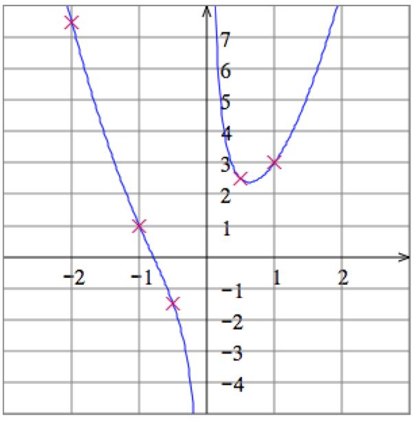
2. Using the table: a. 𝑓 ( 1) = 4 b. 𝑓 (1) = 1

3. Using the table: a. 𝑓 (2) 𝑓 ( 2) = 0.5 2 = 2.5 b. 𝑓 ( 1)𝑓 ( 2) = (4)(2) = 8 c. 2𝑓 ( 1) = 2(4) = 8

4. Using the table: a. 𝑓 (1) 𝑓 ( 1) = 1 4 = 5 b. 𝑓 (1)𝑓 ( 2) = ( 1)(2) = 2 c. 3𝑓 ( 2) = 3(2) = 6

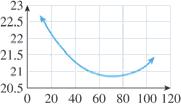
5. From the graph, we estimate: a. 𝑓 (1) = 20 b. 𝑓 (2) = 30

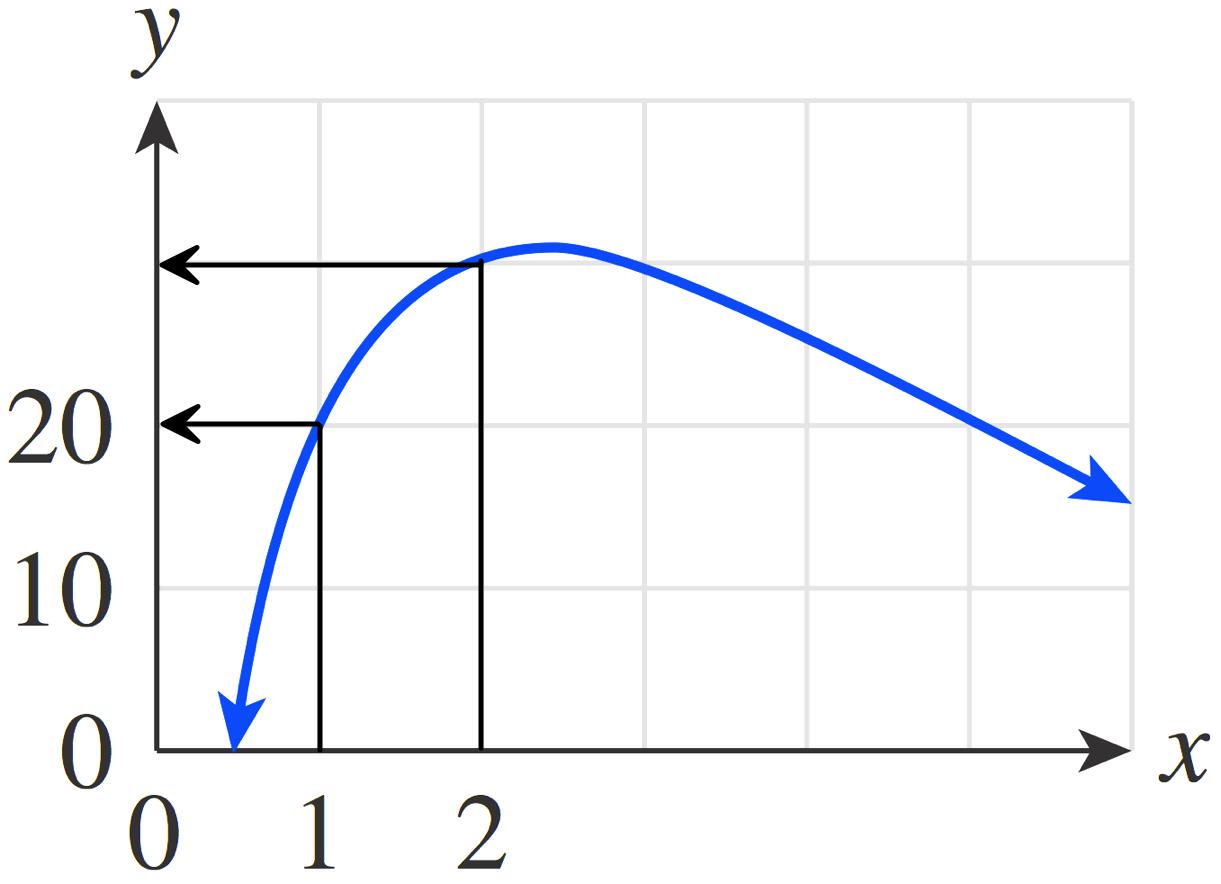
In a similar way, we find: c. 𝑓 (3) = 30 d. 𝑓 (5) = 20\\e. 𝑓 (3) 𝑓 (2) = 30 30 = 0 f. 𝑓 (3 2) = 𝑓 (1) = 20

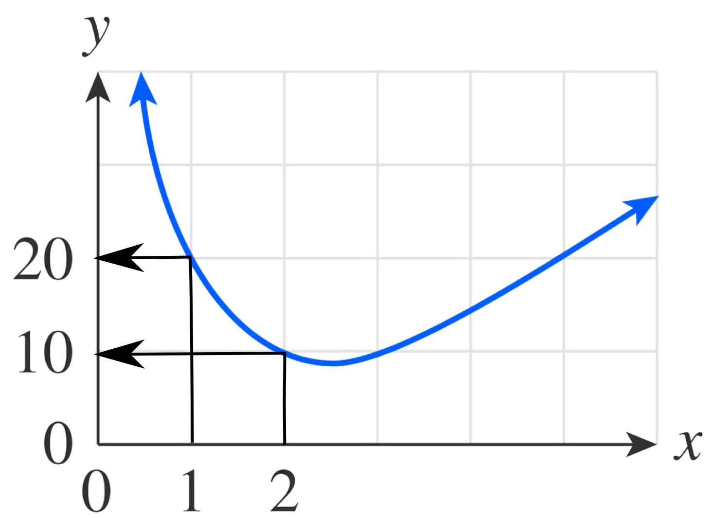
6. From the graph, we estimate: a. 𝑓 (1) = 20 b. 𝑓 (2) = 10 In a similar way, we find: c. 𝑓 (3) = 10 d. 𝑓 (5) = 20 \\e. 𝑓 (3) 𝑓 (2) = 10 10 = 0 f. 𝑓 (3 2) = 𝑓 (1) = 20

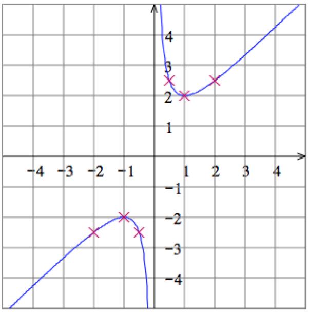
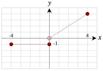
7. From the graph, we estimate: a. 𝑓 ( 1) = 0 b. 𝑓 (1) = 3 since the solid dot is on (1, 3).

In a similar way, we estimate c. 𝑓 (3) = 3 d. Since 𝑓 (3) = 3 and 𝑓 (1) = 3, 𝑓 (3) 𝑓 (1) 3 1 = 3 ( 3) 3 1 = 3.

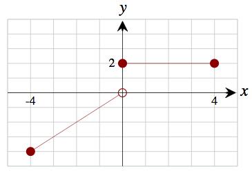
8. From the graph, we estimate: a. 𝑓 ( 3) = 3 b. 𝑓 ( 1) = 2 since the solid dot is on ( 1, 2)

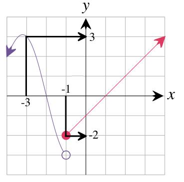
In a similar way, we estimate c. 𝑓 (1) = 0

d. Since 𝑓 (3) = 2 and 𝑓 (1) = 0, 𝑓 (3) 𝑓 (1) 3 1 = 2 0 3 1 = 1

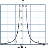
9. 𝑓 (𝑥) = 𝑥 1 𝑥 2 , with its natural domain.

The natural domain consists of all 𝑥 for which 𝑓 (𝑥) makes sense: all real numbers other than 0

a. Since 4 is in the natural domain, 𝑓 (4) is defined, and 𝑓 (4) = 4 1 4 2 = 4 1 16 = 63 16

b. Since 0 is not in the natural domain, 𝑓 (0) is not defined.

c. Since 1 is in the natural domain, 𝑓 ( 1) = 1 1 ( 1) 2 = 1 1 1 = 2

10. 𝑓 (𝑥) = 2 𝑥 𝑥 2 , with domain [2, ∞)

a. Since 4 is in [2, ∞), 𝑓 (4) is defined, and 𝑓 (4) = 2 4 4 2 =

b. Since 0 is not in [2, ∞), 𝑓 (0) is not defined. c. Since 1 is not in [2, ∞), 𝑓 (1) is not defined.

11. 𝑓 (𝑥) = 𝑥 + 10 √ , with domain [ 10, 0)

a. Since 0 is not in [ 10, 0), 𝑓 (0) is not defined. b. Since 9 is not in [ 10, 0), 𝑓 (9) is not defined.

c. Since 10 is in [ 10, 0), 𝑓 ( 10) is defined, and 𝑓 ( 10) = 10 + 10 √ = 0√ = 0

12. 𝑓 (𝑥) = 9 𝑥 2 √ , with domain ( 3, 3)

a. Since 0 is in ( 3, 3), 𝑓 (0) is defined, and 𝑓 (0) = 9 0 √ = 3

b. Since 3 is not in ( 3, 3), 𝑓 (3) is not defined. c. Since 3 is not in ( 3, 3), 𝑓 ( 3) is not defined.

13. 𝑓 (𝑥) = 4𝑥 3

a. 𝑓 ( 1) = 4( 1) 3 = 4 3 = 7 b. 𝑓 (0) = 4(0) 3 = 0 3 = 3

c. 𝑓 (1) = 4(1) 3 = 4 3 = 1 d. Substitute 𝑦 for 𝑥 to obtain 𝑓 (𝑦) = 4𝑦 3

e. Substitute (𝑎 + 𝑏) for 𝑥 to obtain 𝑓 (𝑎 + 𝑏) = 4(𝑎 + 𝑏) 3.

14. 𝑓 (𝑥) = 3𝑥 + 4

a. 𝑓 ( 1) = 3( 1) + 4 = 3 + 4 = 7 b. 𝑓 (0) = 3(0) + 4 = 0 + 4 = 4

c. 𝑓 (1) = 3(1) + 4 = 3 + 4 = 1 d. Substitute 𝑦 for 𝑥 to obtain 𝑓 (𝑦) = 3𝑦 + 4

e. Substitute (𝑎 + 𝑏) for 𝑥 to obtain 𝑓 (𝑎 + 𝑏) = 3(𝑎 + 𝑏) + 4.

15. 𝑓 (𝑥) = 𝑥 2 + 2𝑥 + 3

a. 𝑓 (0) = (0) 2 + 2(0) + 3 = 0 + 0 + 3 = 3 b. 𝑓 (1) = 1 2 + 2(1) + 3 = 1 + 2 + 3 = 6

Solutions Section 1.1

c. 𝑓 ( 1) = ( 1) 2 + 2( 1) + 3 = 1 2 + 3 = 2 d. 𝑓 ( 3) = ( 3) 2 + 2( 3) + 3 = 9 6 + 3 = 6

e. Substitute 𝑎 for 𝑥 to obtain 𝑓 (𝑎) = 𝑎 2 + 2𝑎 + 3. f. Substitute (𝑥 + ℎ) for 𝑥 to obtain 𝑓 (𝑥 + ℎ) = (𝑥 + ℎ) 2 + 2(𝑥 + ℎ) + 3.

16. 𝑔(𝑥) = 2𝑥 2 𝑥 + 1

a. 𝑔(0) = 2(0) 2 0 + 1 = 0 0 + 1 = 1 b. 𝑔( 1) = 2( 1) 2 ( 1) + 1 = 2 + 1 + 1 = 4

c. Substitute 𝑟 for 𝑥 to obtain 𝑔(𝑟) = 2𝑟 2 𝑟 + 1

d. Substitute (𝑥 + ℎ) for 𝑥 to obtain 𝑔(𝑥 + ℎ) = 2(𝑥 + ℎ) 2 (𝑥 + ℎ) + 1

17. 𝑔(𝑠) = 𝑠 2 + 1 𝑠

a. 𝑔(1) = 1 2 + 1 1 = 1 + 1 = 2 b. 𝑔( 1) = ( 1) 2 + 1 1 = 1 1 = 0

c. 𝑔(4) = 4 2 + 1 4 = 16 + 1 4 = 65 4 or 16.25 d. Substitute 𝑥 for 𝑠 to obtain 𝑔(𝑥) = 𝑥 2 + 1 𝑥

e. Substitute (𝑠 + ℎ) for 𝑠 to obtain 𝑔(𝑠 + ℎ) = (𝑠 + ℎ) 2 + 1 𝑠 + ℎ

f. 𝑔(𝑠 + ℎ) 𝑔(𝑠) = Answer to part (e) Original function = !(𝑠 + ℎ) 2 + 1 𝑠 + ℎ " !𝑠 2 + 1 𝑠 "

18. ℎ(𝑟) = 1 𝑟 + 4

a. ℎ(0) = 1 0 + 4 = 1 4 b. ℎ( 3) = 1 ( 3) + 4 = 1 1 = 1

c. ℎ( 5) = 1 ( 5) + 4 = 1 ( 1) = 1 d. Substitute 𝑥 2 for 𝑟 to obtain ℎ(𝑥 2) = 1 𝑥 2 + 4 .

e. Substitute (𝑥 2 + 1) for 𝑟 to obtain ℎ(𝑥 2 + 1) = 1 (𝑥 2 + 1) + 4 = 1 𝑥 2 + 5

f. ℎ(𝑥 2) + 1 = Answer to part (d) + 1 = 1 𝑥 2 + 4 + 1\\

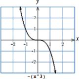
19. 𝑓 (𝑥) = 𝑥 3 (domain ( ∞, ∞)) Technology formula: -(x^3)\\

20. 𝑓 (𝑥) = 𝑥 3 (domain [0, ∞)) Technology formula: x^3

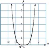
21. 𝑓 (𝑥) = 𝑥 4 (domain ( ∞, ∞)) Technology formula: x^4

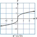
22. 𝑓 (𝑥) = 𝑥 3 √ (domain ( ∞, ∞)) Technology formula: x^(1/3)

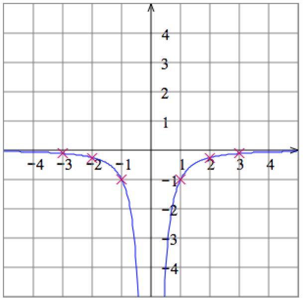
23. 𝑓 (𝑥) = 1 𝑥 2 (𝑥 ≠ 0) Technology formula: 1/(x^2)

24. 𝑓 (𝑥) = 𝑥 + 1 𝑥 (𝑥 ≠ 0) Technology formula: x+1/x

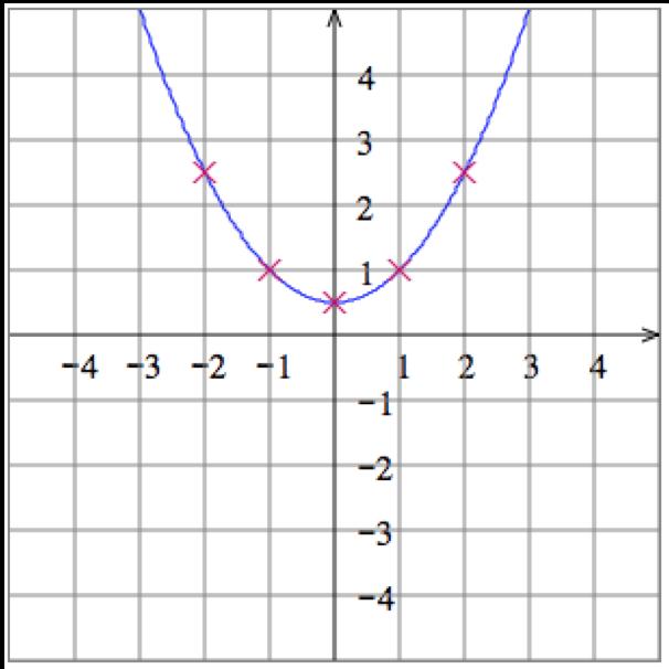
25. a. 𝑓 (𝑥) = 𝑥 ( 1 ≤ 𝑥 ≤ 1)

Since the graph of 𝑓 (𝑥) = 𝑥 is a diagonal 45 ∘ line through the origin inclining up from left to right, the correct graph is (A).

b. 𝑓 (𝑥) = 𝑥 ( 1 ≤ 𝑥 ≤ 1)

Since the graph of 𝑓 (𝑥) = 𝑥 is a diagonal 45 ∘ line through the origin inclining down from left to right, the correct graph is (D).

c. 𝑓 (𝑥) = √𝑥 (0 < 𝑥 < 4)

Since the graph of 𝑓 (𝑥) = √𝑥 is the top half of a sideways parabola, the correct graph is (E).

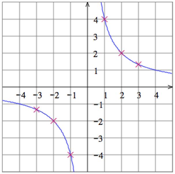
d. 𝑓 (𝑥) = 𝑥 + 1 𝑥 2 (0 < 𝑥 < 4)

If we plot a few points like 𝑥 = 1∕2, 1, 2, and 3, we find that the correct graph is (F).

e. 𝑓 (𝑥) = |𝑥| ( 1 ≤ 𝑥 ≤ 1)

Since the graph of 𝑓 (𝑥) = |𝑥|is a "V"-shape with its vertex at the origin, the correct graph is (C).

f. 𝑓 (𝑥) = 𝑥 1 ( 1 ≤ 𝑥 ≤ 1)

Solutions Section 1.1

Since the graph of 𝑓 (𝑥) = 𝑥 1 is a straight line through (0, 1) and (1, 0), the correct graph is (B).

26. a. 𝑓 (𝑥) = 𝑥 + 3 (0 < 𝑥 ≤ 3)

Since the graph of 𝑓 (𝑥) = 𝑥 + 3 is a straight line inclining down from left to right, the correct graph must be (D).

b. 𝑓 (𝑥) = 2 |𝑥| ( 2 < 𝑥 ≤ 2)

Since 𝑓 (𝑥) = 2 |𝑥| is obtained from the graph of 𝑦 = |𝑥| by flipping it vertically (the minus sign in front of |𝑥|) and then moving it 2 units vertically up (adding 2 to all the values), the correct graph is (F).

c. 𝑓 (𝑥) = 𝑥 + 2 √ ( 2 < 𝑥 ≤ 2)

The graph of𝑓 (𝑥) = 𝑥 + 2 √ is similar to that of 𝑦 = √𝑥, which is half a parabola on its side, and the correct graph is (A).

d. 𝑓 (𝑥) = 𝑥 2 + 2 ( 2 < 𝑥 ≤ 2)

The graph of 𝑓 (𝑥) = 𝑥 2 + 2 is a parabola opening down, so the correct graph is (C).

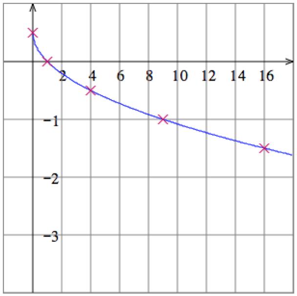
e. 𝑓 (𝑥) = 1 𝑥 1

The graph of 𝑓 (𝑥) = 1 𝑥 1 (0 < 𝑥 ≤ 3) is part of a hyperbola, and the correct graph is (E).

f. 𝑓 (𝑥) = 𝑥 2 1 ( 2 < 𝑥 ≤ 2)

The graph of 𝑓 (𝑥) = 𝑥 2 1 is a parabola opening up, so the correct graph is (B).

27. Technology formula: 0.1*x^2 - 4*x+5

Table of values:

)

28. Technology formula: 0.4*x^2-6*x-0.1

Table of values:

29. Technology formula: (x^2-1)/(x^2+1)

Table of values:

(𝑥)

30. Technology formula: (2*x^2+1)/(2*x^2-1)

Table of values:

31. 𝑓 (𝑥) = {𝑥 if 4 ≤ 𝑥 < 0 2 if 0 ≤ 𝑥 ≤ 4

Technology formula: x*(x\lt 0)+2*(x\gt

a. 𝑓 ( 1) = 1 We used the first formula, since 1 is in [ 4, 0)

b. 𝑓 (0) = 2. We used the second formula, since 0 is in [0, 4].

c. 𝑓 (1) = 2 We used the second formula, since 1 is in [0, 4].

32. 𝑓 (𝑥) = { 1 if 4 ≤ 𝑥 ≤ 0 𝑥 if 0 < 𝑥 ≤ 4

Technology formula: (-1)*(x\lt =0)+x*(x\gt 0) (For a graphing calculator, use ≤ instead of <=.)

a. 𝑓 ( 1) = 1 We used the first formula, since 1 is in [ 4, 0]

b. 𝑓 (0) = 1. We used the first formula, since 0 is in [ 4, 0].

c. 𝑓 (1) = 1 We used the second formula, since 1 is in (0, 4].

33. 𝑓 (𝑥) = ⎧ ⎨ ⎩ ⎪ ⎪ 𝑥 2 if 2 < 𝑥 ≤ 0 1 𝑥 if 0 < 𝑥 ≤ 4

Technology formula: (x^2)*(x<=0)+(1/x)*(0<x) (For a graphing calculator, use ≤ instead of <=.)

a. 𝑓 ( 1) = 1 2 = 1 We used the first formula, since 1 is in ( 2, 0]

b. 𝑓 (0) = 0 2 = 0 We used the first formula, since 0 is in ( 2, 0]

c. 𝑓 (1) = 1∕1 = 1. We used the second formula, since 1 is in (0, 4].

34. 𝑓 (𝑥) = { 𝑥 2 if 2 < 𝑥 ≤ 0

√𝑥 if 0 < 𝑥 < 4

Technology formula: Excel: (-1\*x^2)\*(x\lt =0)+SQRT(ABS(x))\*(x\gt 0)

TI-83/84 Plus: (-1\*x^2)\*(x≤0)+ √(x)\*(x\gt 0)

a. 𝑓 ( 1) = ( 1) 2 = 1 We used the first formula, since 1 is in ( 2, 0]

b. 𝑓 (0) = 0 2 = 0 We used the first formula, since 0 is in ( 2, 0]

c. 𝑓 (1) = 1√ = 1 We used the second formula, since 1 is in (0, 4).

35. 𝑓 (𝑥) = ⎧ ⎨

𝑥 if 1 < 𝑥 ≤ 0

𝑥 + 1 if 0 < 𝑥 ≤ 2

𝑥 if 2 < 𝑥 ≤ 4

Technology formula: x*(x<=0)+(x+1)*(0<x)*(x<=2)+x*(2<x) (For a graphing calculator, use ≤ instead of <=.)

a. 𝑓 (0) = 0. We used the first formula, since 0 is in ( 1, 0].

b. 𝑓 (1) = 1 + 1 = 2 We used the second formula, since 1 is in (0, 2]

c. 𝑓 (2) = 2 + 1 = 3. We used the second formula, since 2 is in (0, 2].

d. 𝑓 (3) = 3 We used the third formula, since 3 is in (2, 4]

36. 𝑓 (𝑥) = ⎧ ⎨

𝑥 if 1 < 𝑥 < 0

𝑥 2 if 0 ≤ 𝑥 ≤ 2

𝑥 if 2 < 𝑥 ≤ 4

Technology formula: x*(x\lt 0)+(x-2)*(0\lt =x)*(x\lt =2)+(-x)*(2\lt x) (For a graphing calculator, use ≤ instead of <=.)

Solutions Section 1.1

a. 𝑓 (0) = 0 2 = 2 We used the second formula, since 0 is in [0, 2]

b. 𝑓 (1) = 1 2 = 1. We used the second formula, since 1 is in [0, 2].

c. 𝑓 (2) = 2 2 = 0 We used the second formula, since 2 is in [0, 2]

d. 𝑓 (3) = 3. We used the third formula, since 3 is in (2, 4].

37. 𝑓 (𝑥) = 𝑥 2

a. 𝑓 (𝑥 + ℎ) = (𝑥 + ℎ) 2 Therefore, 𝑓 (𝑥 + ℎ) 𝑓 (𝑥) = (𝑥 + ℎ) 2 𝑥 2 = 𝑥 2 + 2𝑥ℎ + ℎ 2 𝑥 2 = 2𝑥ℎ + ℎ 2 = ℎ(2𝑥 + ℎ)

b. Using the answer to part (a), 𝑓 (𝑥 + ℎ) 𝑓 (𝑥) ℎ = ℎ(2𝑥 + ℎ) ℎ = 2𝑥 + ℎ

38. 𝑓 (𝑥) = 3𝑥 1

a. 𝑓 (𝑥 + ℎ) = 3(𝑥 + ℎ) 1 = 3𝑥 + 3ℎ 1 Therefore, 𝑓 (𝑥 + ℎ) 𝑓 (𝑥) = 3𝑥 + 3ℎ 1 (3𝑥 1) = 3𝑥 + 3ℎ 1 3𝑥 + 1 = 3ℎ

b. Using the answer to part (a), 𝑓 (𝑥 + ℎ) 𝑓 (𝑥) ℎ = 3ℎ ℎ = 3

39. 𝑓 (𝑥) = 2 𝑥 2

a. 𝑓 (𝑥 + ℎ) = 2 (𝑥 + ℎ) 2 Therefore, 𝑓 (𝑥 + ℎ) 𝑓 (𝑥) = 2 (𝑥 + ℎ) 2 (2 𝑥 2) = 2 𝑥 2 2𝑥ℎ ℎ 2 2 + 𝑥 2 = 2𝑥ℎ ℎ 2 = ℎ(2𝑥 + ℎ)

b. Using the answer to part (a), 𝑓 (𝑥 + ℎ) 𝑓 (𝑥) ℎ = ℎ(2𝑥 + ℎ) ℎ = (2𝑥 + ℎ)

40. 𝑓 (𝑥) = 𝑥 2 + 𝑥 a. 𝑓 (𝑥 + ℎ) = (𝑥 + ℎ) 2 + (𝑥 + ℎ)Therefore, 𝑓 (𝑥 + ℎ) 𝑓 (𝑥) = (𝑥 + ℎ) 2 + (𝑥 + ℎ) (𝑥 2 + 𝑥) = 𝑥 2 + 2𝑥ℎ + ℎ 2 + 𝑥 + ℎ 𝑥 2 𝑥 = 2𝑥ℎ + ℎ 2 + ℎ = ℎ(2𝑥 + ℎ + 1)

b. Using the answer to part (a), 𝑓 (𝑥 + ℎ) 𝑓 (𝑥) ℎ = ℎ(2𝑥 + ℎ + 1) ℎ = 2𝑥 + ℎ + 1

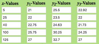
41. From the table,

a. 𝑝(2) = 0.67; Pemex produced 0.67 billion barrels of crude oil in 2017 (𝑡 = 2).

𝑝(3) = 0.61; Pemex produced 0.61 billion barrels of crude oil in 2018 (𝑡 = 3).

𝑝(6) = 0.62; Pemex produced 0.62 billion barrels of crude oil in 2021 (𝑡 = 6).

Solutions Section 1.1

b. 𝑝(6) 𝑝(3) = 0 62 0 61 = 0 01; Annual crude oil production by Pemex increased by 0.01 billion barrels from 2018 (𝑡 = 3) to 2021 (𝑡 = 6).

42. From the table,

a. 𝑠(0) = 0.69; Pemex produced 0.69 billion barrels of offshore crude oil in 2015 (𝑡 = 0).

𝑠(2) = 0.56; Pemex produced 0.56 billion barrels of offshore crude oil in 2017 (𝑡 = 2).

𝑠(4) = 0.51; Pemex produced 0.51 billion barrels of offshore crude oil in 2019 (𝑡 = 4).

b. 𝑠(4) 𝑠(0) = 0.51 0.69 = 0.18; Annual offshore crude oil production by Pemex decreased by 0.18 billion barrels from 2015 (𝑡 = 0) to 2019 (𝑡 = 4).

43. a. Graph of 𝑝:

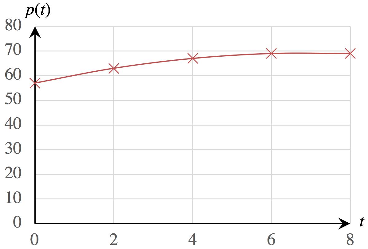
The graph suggests a curve, so we exclude the linear models (A) and (C). Model (B) gives a parabola that curves up whereas the curve suggested by the graph curves down, leaving us with Model (D). Also, model (D) gives almost the exact values shown in the chart. (Use the technology formula -0.25x^2+3.5x+57.)

b. Using Model (D), 𝑝(5) = 0.25(5) 2 + 3.5(5) + 57 = 68.25

Interpretation: 𝑡 = 5 represents 5 years since the start of 2013, or the start of 2018. Thus, we interpret the answer as follows: Approximately 68.25% of U.S. adults used Facebook at the start of 2018

c. The graph becomes less steep as time increases, indicating decelerating Facebook membership over the period 2013–2021.

44. a. Graph of 𝑝:

The graph suggests a curve, so we exclude the linear model (B). Model (D) gives a parabola that curves up whereas the curve suggested by the graph curves down, leaving us with Models (A) and (C). Model (A) gives values that round to the values shown in the chart wheeras Model (C) is way off. (Use the technology formula -0.32x^2+3.6x+13

b. Using Model (A), 𝑝(7 5) = 0 32(7 5) 2 + 3 6(7 5) + 13 = 22

Interpretation: 𝑡 = 7.5 represents 7.5 years since the start of 2013, or midway through 2020. Thus, we interpret the answer as follows: Approximately 22% of U.S. adults used Twitter midway through 2020.

c. The graph becomes less steep as time increases, indicating decelerating Twitter membership over the period 2013–2021.

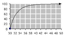
45. From the graph, 𝑓 (11) ≈ 800. Because 𝑓 is the number of thousands of housing starts in year 11, we interpret the result as follows: Approximately 800,000 homes were started in 2016. Similarly, 𝑓 (15) ≈ 1,000 Approximately 1,000,000 homes were started in 2020. Also, we estimate 𝑓 (2.5) ≈ 800. Because 𝑡 = 2.5 is midway between 2007 and 2008, we interpret the result as follows: approximately 800,000 homes were started in the year beginning midway through 2007.

46. From the graph, 𝑓 (3) ≈ 600 Because 𝑓 is the number of thousands of housing starts in year 3, we interpret the result as follows: Approximately 600,000 homes were started in 2008.

𝑓 (12) ≈ 900: Approximately 900,000 homes were started in 2016.

𝑓 (14 5) ≈ 950: Approximately 950,000 homes were started in the year beginning midway through 2019.

47. 𝑓 (14 10) = 𝑓 (4) ≈ 400. Interpretation: Approximately 400,000 homes were started in 2009 (𝑡 = 4). 𝑓 (14) 𝑓 (10) ≈ 900 700 = 200 Interpretation: 𝑓 (14) 𝑓 (10) is the change in the number of housing starts (in thousands) from 2015 to 2019; there were approximately 200,000 more housing starts in 2019 than in 2015.

48. 𝑓 (15 1) = 𝑓 (14) ≈ 900. Interpretation: Approximately 900,000 homes were started in 2019 (𝑡 = 14)

𝑓 (15) 𝑓 (1) ≈ 1,000 1,500 = 500. Interpretation: 𝑓 (15) 𝑓 (1) is the change in the number of housing starts (in thousands) from 2006 to 2020; there were approximately 500,000 fewer housing starts in 2020 than in 2006.

49. 𝑓 (𝑡 + 5) 𝑓 (𝑡) measures the change from year 𝑡 to the year five years later. It is greatest when the line segment from year 𝑡 to year 𝑡 + 5 is steepest upward-sloping. From the graph, or by computing differences of values estimated from the graph, this occurs when 𝑡 = 6 or 7:

𝑓 (11) 𝑓 (6) = 800 400 = 400; 𝑓 (12) 𝑓 (7) = 900 500 = 400

Interpretation: The greatest five-year increase in the number of housing starts occurred in 2011–2016 and again in 2012–2017.

50. 𝑓 (𝑡) 𝑓 (𝑡 1) measures the change from year 𝑡 1 to the following year. It is least when the the line segment from year 𝑡 1 to year 𝑡 is steepest downward-sloping. From the graph, this occurs when 𝑡 = 2, for a change of 𝑓 (2) 𝑓 (1) = 1,000 1,500 = 500

Interpretation: The greatest annual decrease in the number of housing starts occurred in 2006–2007.

51. a. From the graph, 𝑏(3) ≈ 50 and 𝑏(5) ≈ 35. The (50-day average) price of Bitcoin was approximately $50,000 on June 1, 2021 (𝑡 = 3) and $35,000 on August 1, 2021 (𝑡 = 5). 𝑏(7) 𝑏(5) ≈ 50 35 = 15. The Bitcoin price increased by around $15,000 from August 1 to October 1, 2021.

b. Increasing most rapidly when the graph is steepest upward from left to right on the interal [1, 3], which occurs at 𝑡 = 1 (integer answer required). Thus, during the period April 1–June 1, 2021, the price of Bitcoin was increasing most rapidly around April 1.

c. Decreasing most rapidly when the graph is steepest down from left to right, which occurs at 𝑡 = 3 (integer answer required). Thus, during the period April 1–June 1, 2021, the price of Butcoin was decreasing most rapidly around June 1.

52. a. From the graph, 𝑒(2) ≈ 2 5 and 𝑒(4) ≈ 2 5. The price of Etherium was approximately $2,500 on May 1, 2021 (𝑡 = 2) and again on July 1, 2021 (𝑡 = 4) .

𝑒(3) 𝑒(1) ≈ 2 3 = 1. The price of Etherium decreased by around $1,000 from April 1 to June 1, 2021.

b. Increasing most rapidly when the graph is steepest upward from left to right on the interal [1, 5], which occurs at 𝑡 = 4 (integer answer required). Thus, during the period April 1–August 1, 2021, the price of Etherium was increasing most rapidly around July 1.

c. Decreasing most rapidly when the graph is steepest down from left to right, which occurs at 𝑡 = 2 (integer answer required). Thus, during the period April 1–August 1, 2021, the price of Etherium was decreasing most rapidly around May 1.

53. 𝑟(𝑥) = 0.4𝑥 2 + 𝑥 + 26.5 (0 ≤ 𝑥 ≤ 5)

a. The domain of 𝑟 is [0, 5]

Solutions Section 1.1

𝑟(0) = 0.4(0) 2 + 0 + 26.5 = 26.5;

𝑟(1) = 0.4(1) 2 + 1 + 26.5 = 27.9

𝑟(3) = 0.4(3) 2 + 3 + 26.5 = 33.1

𝑟(5) = 0 4(5) 2 + 5 + 26 5 = 41 5

Food delivery app revenues in the U.S. were projected to be $26.5 billion in 2020, $27.9 billion in 2021, $33.1 billion in 2023, and $41.5 billion in 2025.

b. Graph:

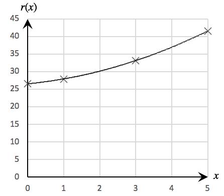
(As the curve is concave up the projected revenue was accelerating.)

54. 𝑟(𝑥) = 0.2𝑥 2 + 3𝑥 + 18 (0 ≤ 𝑥 ≤ 5)

a. The domain of 𝑟 is [0, 5]

𝑟(0) = 0 2(0) 2 + 3(0) + 18 = 18;

𝑟(1) = 0 2(1) 2 + 3(1) + 18 = 20 8

𝑟(3) = 0 2(3) 2 + 3(3) + 18 = 25 2

𝑟(5) = 0 2(5) 2 + 3(5) + 18 = 28

Food delivery app revenues in Europe were projected to be $18 billion in 2020, $20.8 billion in 2021, $25.2 billion in 2023, and $28 billion in 2025.

b. Graph

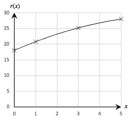
(As the graph is concave down the projected revenue was decelerating).

55. a. The model is valid for the range 1958 (𝑡 = 0) through 1966 (𝑡 = 8). Thus, an appropriate domain is [0, 8]. 𝑡 ≥ 0 is not an appropriate domain because it would predict federal funding of NASA beyond 1966, whereas the model is based only on data up to 1966.

b. 𝑝(𝑡) = 4.5

1 07 (𝑡 8) 2

⇒ 𝑝(5) = 4 5 1.07 (5 8) 2 ≈ 2 4 Technology formula: 4.5/(1.07^((t-8)^2))

𝑡 = 5 represents 1958 + 5 = 1963, and therefore we interpret the result as follows: In 1963, 2.4% of the U.S. federal budget was allocated to NASA.

c. 𝑝(𝑡) is increasing most rapidly when the graph is steepest upward-sloping from left to right, and, among the given values of 𝑡, this occurs when 𝑡 = 5. Thus, the percentage of the budget allocated to NASA was 42

Solutions Section 1.1 increasing most rapidly in 1963.

56. a. [1, 55]; [0, 55] is not an appropriate domain because 𝑝 is undefined at 0

b. 𝑝(𝑡) = 0 03 + 5 𝑡 0 6

⇒ 𝑝(40) = 0 03 + 5 40 0 6 ≈ 0 58 Technology formula: 0.03+5/t^0.6

𝑡 = 40 represents 1965 + 40 = 2005, and therefore we interpret the result as follows: In 2005, 0.58% of the US federal budget was allocated to NASA.

c. If we evaluate 𝑝(𝑡) for 𝑡 = 100, 1,000, 100,000, 1,000,000 . . . , we find values of 𝑝(𝑡) decreasing toward 0.03. Thus, in the (very) long term, the percentage of the budget allocated to NASA is predicted to approach 0.03%

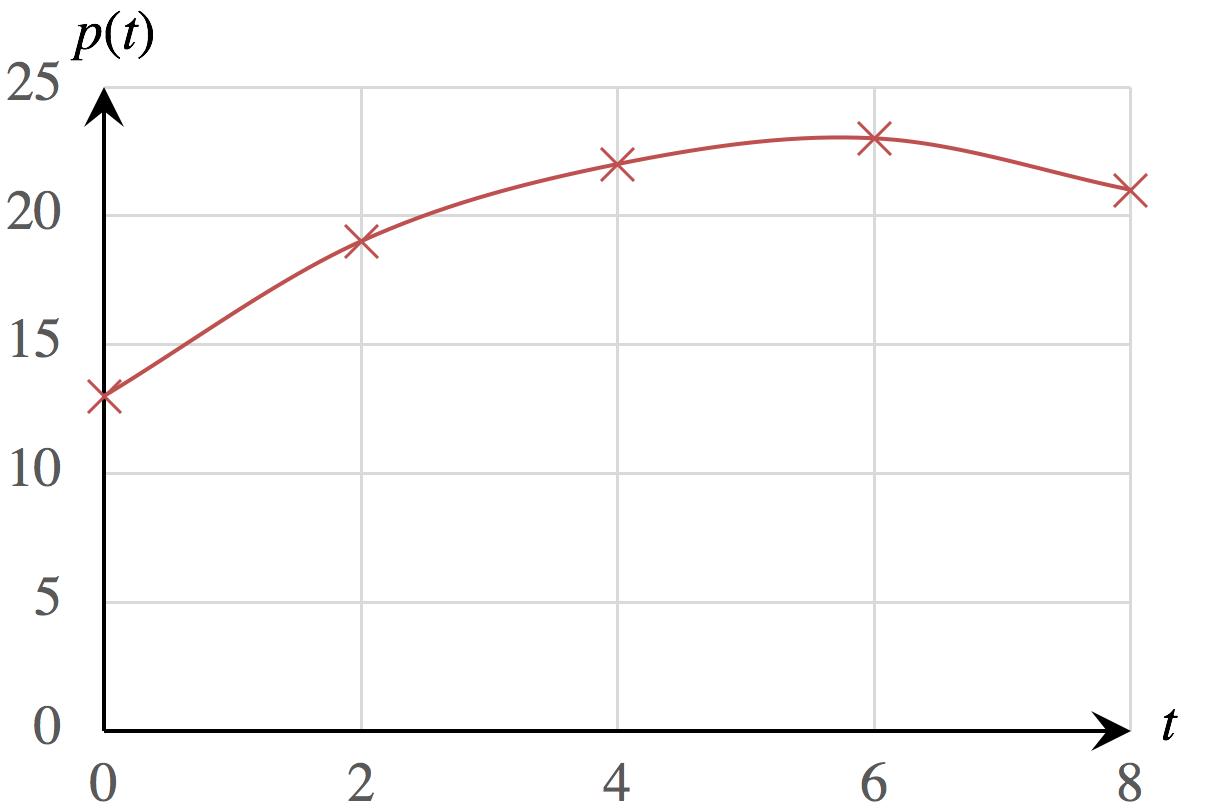
57. a. 𝑝(𝑡) = 100⎛ ⎝ ⎜1 12, 200 𝑡 4 48 ⎞ ⎠ ⎟ (𝑡 ≥ 8.5)

Technology formula: 100*(1-12200/t^4.48)

b. Graph:

c. Table of values:

d. From the table, 𝑝(12) = 82.2, so that 82.2% of children are able to speak in at least single words by the age of 12 months.

e. We seek the first value of 𝑡 such that 𝑝(𝑡) is at least 90. Since 𝑡 = 14 has this property ( 𝑝(14) = 91 1) we conclude that, at 14 months, 90% or more children are able to speak in at least single words.

58. a. 𝑝(𝑡) = 100!1 5 27 × 10 17 𝑡 12 " (𝑡 ≥ 30)

Technology formula: 100*(1-5.27*10^17/t^12)

b.Graph:

c. Table of values:

d. From the table, 𝑝(36) = 88 9, so that 88.9% of children are able to speak in sentences of five or more words by the age of 36 months.

Solutions Section 1.1

e. We seek the first value of 𝑡 such that 𝑝(𝑡) is at least 75. Since 𝑡 = 34 has this property ( 𝑝(34) = 77 9) we conclude that, at 34 months, 75% or more children are able to speak in sentences of five or more words.

59. 𝑣(𝑡) = ⎧ ⎨ ⎩ ⎪ ⎪

8(1 22) 𝑡 if 0 ≤ 𝑡 < 16

400𝑡 6,200 if 16 ≤ 𝑡 < 25

0.45(𝑡 25) 3 + 3,800 if 25 ≤ 𝑡 ≤ 40

a. 𝑣(10) = 8(1.22) 10 ≈ 58. We used the first formula, since 10 is in [0, 16).

𝑣(16) = 400(16) 6,200 = 200 We used the second formula, since 16 is in [16, 25)

𝑣(40) = 0 45(40 25) 3 + 3,800 ≈ 5,319 We used the third formula, since 40 is in [25, 40]

Interpretation: Processor speeds were about 58 MHz in 1990, 200 MHz in 1996, and 5,319 MHz in 2020.

b. Technology formula (using 𝑥 as the independent variable):

(8*(1.22)^x)*(x<16)+(400*x-6200)*(x>=16)*(x<25) +(0.45*(x-25)^3+3800)*(x>=25)

(For a graphing calculator, use ≤ instead of <=.)

c. Using the above technology formula (for instance, on the Function Evaluator and Grapher on the Web site) we obtain the graph and table of values.

Graph:

Table of values:

𝑡

𝑣(𝑡) 8 18

d. From either the graph or the table, we see that the speed reached 3,000 MHz between 𝑡 = 20 and 𝑡 = 24. We can obtain a more precise answer algebraically by using the formula for the corresponding portion of the graph:

3,000 = 400𝑡 6,200 giving

𝑡 = 9,200

400 = 23

Since 𝑡 is time since 1980, 𝑡 = 23 corresponds to 2003.

60. 𝑣(𝑡) = ⎧ ⎨ ⎩ ⎪ ⎪ 0 12𝑡 2 + 0 04𝑡 + 0 2 if 0 ≤ 𝑡 < 12 1 1(1 22) 𝑡 if 12 ≤ 𝑡 < 26

400𝑡 10,200 if 26 ≤ 𝑡 ≤ 30

a. 𝑣(2) = 0 12(2) 2 + 0 04(2) + 0 2 = 0 76 We used the first formula, since 2 is in [0, 12)

𝑣(12) = 1 1(1 22) 12 ≈ 12 We used the second formula, since 12 is in [12, 26)

𝑣(28) = 400(28) 10, 200 = 1, 000. We used the third formula, since 28 is in [26, 30].

Interpretation: Processor speeds were about 0.76 MHz in 1972, 12 MHz in 1982, and 1,000 MHz in 1998.

b. Technology formula (using 𝑥 as the independent variable): (0.12*x^2+0.04*x+0.2)*(x<12)+(1.1*(1.22)^x)*(x>=12)*(x<26) +(400*x-10200)*(x>=26)

(For a graphing calculator, use ≤ instead of <=.)

c. Using the above technology formula (for instance, on the Function Evaluator and Grapher on the Web site) we obtain the graph and table of values.

Graph:

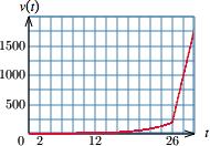
Table of values:

d. From either the graph or the table, we see that the speed reached 500 MHz around 𝑡 = 27 We can obtain a more precise answer algebraically by using the formula for the corresponding portion of the graph:

500 = 400𝑡 10,200

giving

𝑡 = 10,700 400 = 26.75 ≈ 27 to the nearest year

Since 𝑡 is time since 1970, 𝑡 = 27 corresponds to 1997.

61. a. Each row of the table gives us a formula with a condition:

First row in words: 10% of the amount over $0 if your income is over $0 and not over $9,950.

Translation to formula:

0 10𝑥 if 0 < 𝑥 ≤ 9,950

Second row in words: $995.00 + 12% of the amount over $9,950 if your income is over $9,950 and not over $40,525.

Translation to formula:

995 00 + 0 12(𝑥 9, 950) if 9,950 < 𝑥 ≤ 40,525

Continuing in this way leads to the following piecewise-defined function: 𝑇 (𝑥) =

0.10𝑥 if 0 < 𝑥 ≤ 9,950

995 00 + 0 12(𝑥 9,950) if 9,950 < 𝑥 ≤ 40,525 4,664 + 0 22(𝑥 40,525) if 40,525 < 𝑥 ≤ 86,375 14,751 + 0.24(𝑥 86,375) if 86,375 < 𝑥 ≤ 164,925 33,603 + 0.32(𝑥 164,925) if 164,925 < 𝑥 ≤ 209,425 47,843 + 0.35(𝑥 209,425) if 209,425 < 𝑥 ≤ 523,600 157,804 25 + 0 37(𝑥 523,600) if 523,600 < 𝑥

b. A taxable income of $45,000 falls in the bracket 40,525 < 𝑥 ≤ 86,375 and so we use the formula 4,664 + 0.22(𝑥 40,525) : 4,664 + 0 22(45,000 40,525) = 4,664 + 0 22(4,475) = $5,648 50

62. a. Each row of the table gives us a formula with a condition: First row in words: 10% of the amount over $0 if your income is over $0 and not over $8,700.

Translation to formula:

0 10𝑥 if 0 < 𝑥 ≤ 8,700

Second row in words: $870.00 + 15% of the amount over $8,700 if your income is over $8,700 and not over $35,350.

Translation to formula:

870.00 + 0.15(𝑥 8,700) if 8,700 < 𝑥 ≤ 35,350.

Continuing in this way leads to the following piecewise-defined function: 𝑇 (𝑥) =

0 10𝑥 if 0 < 𝑥 ≤ 8,700

870 00 + 0 15(𝑥 8,700) if 8,700 < 𝑥 ≤ 35,350

4,867.50 + 0.22(𝑥 35,350) if 35,350 < 𝑥 ≤ 85,650

17,442.50 + 0.28(𝑥 85,650) if 85,650 < 𝑥 ≤ 178,650

43,482.50 + 0.33(𝑥 178,650) if 178,650 < 𝑥 ≤ 388,350

112,683 50 + 0 35(𝑥 388,350) if 388,350 < 𝑥

b. A taxable income of $45,000 falls in the bracket 35,350 < 𝑥 ≤ 85,650 and so we use the formula 4,867.50 + 0.22(𝑥 35,350) : 4,867 50 + 0 22(45,000 35,350) = 4,867 50 + 0 22(9,650) = $9,990 50

63. The dependent variable is a function of the independent variable. Here, the market price of gold 𝑚 is a function of time 𝑡 Thus, the independent variable is 𝑡 and the dependent variable is 𝑚

64. The dependent variable is a function of the independent variable. Here, the weekly profit 𝑃 is a function of the selling price 𝑠. Thus, the independent variable is 𝑠 and the dependent variable is 𝑃 .

65. To obtain the function notation, write the dependent variable as a function of the independent variable. Thus 𝑦 = 4𝑥 2 2 can be written as 𝑓 (𝑥) = 4𝑥 2 2 or 𝑦(𝑥) = 4𝑥 2 2

66. To obtain the equation notation, introduce a dependent variable instead of the function notation. Thus 𝐶 (𝑡) = 0.34𝑡 2 + 0.1𝑡 can be written as 𝑐 = 0.34𝑡 2 + 0.1𝑡 or 𝑦 = 0.34𝑡 2 + 0.1𝑡

67. False. A graph usually gives infinitely many values of the function while a numerical table will give only a finite number of values.

68. True. An algebraically specified function 𝑓 is specified by algebraic formulas for 𝑓 (𝑥) Given such formulas, we can construct the graph of 𝑓 by plotting the points (𝑥, 𝑓 (𝑥)) for values of 𝑥 in the domain of 𝑓

69. False. In a numerically specified function, only certain values of the function are specified so we cannot know its value on every real number in [0, 10], whereas an algebraically specified function would give values for every real number in [0, 10].

70. False. A graphically specified function is specified by a graph. However, we cannot always expect to find an algebraic formula whose graph is exactly the graph that is given.

71. Functions with infinitely many points in their domain (such as 𝑓 (𝑥) = 𝑥 2) cannot be specified numerically. So, the assertion is false.

72. A numerical model supplies only the values of a function at specific values of the independent variable, whereas an algebraic model supplies the value of a function at every point in its domain. Thus, an algebraic model supplies more information.

73. (Answers may vary.) Take 𝑓 (𝑥) = 𝑥 2. Then

a. 𝑓 (3 + 2) = 𝑓 (5) = 5 2 = 25, whereas 𝑓 (3) + 𝑓 (2) = 3 2 + 2 2 = 9 + 4 = 13. Thus, 𝑓 (3 + 2) ≠ 𝑓 (3) + 𝑓 (2) b. 𝑓 (3 2) = 𝑓 (1) = 1 2 = 1, whereas 𝑓 (3) 𝑓 (2) = 3 2 2 2 = 9 4 = 5. Thus, 𝑓 (3 2) ≠ 𝑓 (3) 𝑓 (2)

74. (Answers may vary.) Take 𝑓 (𝑥) = 𝑥 + 1. Then

a. 𝑓 (3 × 2) = 𝑓 (6) = 6 + 1 = 7, whereas 3𝑓 (2) = 3(2 + 1) = 3 × 3 = 9. Thus, 𝑓 (3 × 2) ≠ 3𝑓 (2).

b. 𝑓 (3 × 2) = 𝑓 (6) = 6 + 1 = 7, whereas 𝑓 (3)𝑓 (2) = (3 + 1)(2 + 1) = 4 × 3 = 12. Thus, 𝑓 (3 × 2) ≠ 𝑓 (3)𝑓 (2).

75. As the text reminds us: to evaluate 𝑓 of a quantity (such as 𝑥 + ℎ) replace 𝑥 everywhere by the whole quantity 𝑥 + ℎ :

𝑓 (𝑥) = 𝑥 2 1 𝑓 (𝑥 + ℎ) = (𝑥 + ℎ) 2 1.

76. Knowing 𝑓 (𝑥) for two values of 𝑥 does not convey any information about 𝑓 (𝑥) at any other value of 𝑥. Interpolation is only a way of estimating 𝑓 (𝑥) at values of 𝑥 not given.

77. If two functions are specified by the same formula 𝑓 (𝑥), say, their graphs must follow the same curve 𝑦 = 𝑓 (𝑥). However, it is the domain of the function that specifies what portion of the curve appears on the graph. Thus, if the functions have different domains, their graphs will be different portions of the curve 𝑦 = 𝑓 (𝑥)

78. If we plot points of the graphs 𝑦 = 𝑓 (𝑥) and 𝑦 = 𝑔(𝑥), we see that, since 𝑔(𝑥) = 𝑓 (𝑥) + 10, we must add 10 to the 𝑦-coordinate of each point in the graph of 𝑓 to get a point on the graph of 𝑔 Thus, the graph of 𝑔 is 10 units higher up than the graph of 𝑓 .

79. Suppose we already have the graph of 𝑓 and want to construct the graph of 𝑔 We can plot a point of the graph of 𝑔 as follows: Choose a value for 𝑥 (𝑥 = 7, say) and then "look back" 5 units to read off 𝑓 (𝑥 5) (𝑓 (2) in this instance). This value gives the 𝑦-coordinate we want. In other words, points on the graph of 𝑔 are obtained by "looking back 5 units" to the graph of 𝑓 and then copying that portion of the curve. Put another way, the graph of 𝑔 is the same as the graph of 𝑓 , but shifted 5 units to the right:

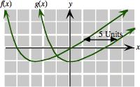
80. Suppose we already have the graph of 𝑓 and want to construct the graph of 𝑔. We can plot a point of

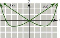
Solutions Section 1.1 the graph of 𝑔 as follows: Choose a value for 𝑥 (𝑥 = 7, say) and then look on the other side of the 𝑦-axis to read off 𝑓 ( 𝑥) (𝑓 ( 7) in this instance). This value gives the 𝑦-coordinate we want. In other words, points on the graph of 𝑔 are obtained by "looking back" to the graph of 𝑓 on the opposite side of the 𝑦-axis and then copying that portion of the curve. Put another way, the graph of 𝑔(𝑥) is the mirror image of the graph of 𝑓 (𝑥) in the 𝑦-axis:

Section 1.2

1. 𝑓 (𝑥) = 𝑥 2 + 1 with domain ( ∞, ∞)

𝑔(𝑥) = 𝑥 1 with domain ( ∞, ∞)

a. 𝑠(𝑥) = 𝑓 (𝑥) + 𝑔(𝑥) = (𝑥 2 + 1) + (𝑥 1) = 𝑥 2 + 𝑥

b. Since both functions are defined for every real number 𝑥, the domain of 𝑠 is the set of all real numbers: ( ∞, ∞)

c. 𝑠( 3) = ( 3) 2 + ( 3) = 9 3 = 6

2. 𝑓 (𝑥) = 𝑥 2 + 1 with domain ( ∞, ∞)

𝑔(𝑥) = 𝑥 1 with domain ( ∞, ∞)

a. 𝑑(𝑥) = 𝑔(𝑥) 𝑓 (𝑥) = (𝑥 1) (𝑥 2 + 1) = 𝑥 2 + 𝑥 2

b. Since both functions are defined for every real number 𝑥, the domain of 𝑑 is the set of all real numbers: ( ∞, ∞).

c. 𝑑( 1) = ( 1) 2 + ( 1) 2 = 4

3. 𝑔(𝑥) = 𝑥 1 with domain ( ∞, ∞)

𝑢(𝑥) = 𝑥 + 10 √ with domain [ 10, 0)

a. 𝑝(𝑥) = 𝑔(𝑥)𝑢(𝑥) = (𝑥 1) 𝑥 + 10 √

b. The domain of 𝑝 consists of all real numbers 𝑥 simultaneously in the domains of 𝑔 and 𝑢; that is, [ 10, 0)

c. 𝑝( 6) = ( 6 1) 6 + 10 √ = ( 7)(2) = 14

4. ℎ(𝑥) = 𝑥 + 4 with domain [10, ∞)

𝑣(𝑥) = 10 𝑥 √ with domain [0, 10]

a. 𝑝(𝑥) = ℎ(𝑥)𝑣(𝑥) = (𝑥 + 4) 10 𝑥 √

b. The domain of 𝑝 consists of all real numbers 𝑥 simultaneously in the domains of ℎ and 𝑣; that is, the single point 𝑥 = 10

c. As 1 is not in the domain of 𝑝, 𝑝(1) is not defined.

5. 𝑔(𝑥) = 𝑥 1 with domain ( ∞, ∞)

𝑣(𝑥) = 10 𝑥 √ with domain [0, 10]

a. 𝑞(𝑥) = 𝑣(𝑥)

𝑔(𝑥) = 10 𝑥 √ 𝑥 1

b. The domain of 𝑞 consists of all real numbers 𝑥 simultaneously in the domains of 𝑣 and 𝑔 such that 𝑔(𝑥) ≠ 0. Since

𝑔(𝑥) = 0 when 𝑥 1 = 0, or 𝑥 = 1

we exclude 𝑥 = 1 from the domain of the quotient. Thus, the domain consists of all 𝑥 in [0, 10] excluding 𝑥 = 1 (since 𝑔(1) = 0), or 0 ≤ 𝑥 ≤ 10; 𝑥 ≠ 1.

c. As 1 is not in the domain of 𝑞, 𝑞(1) is not defined.

6. 𝑔(𝑥) = 𝑥 1 with domain ( ∞, ∞)

𝑣(𝑥) = 10 𝑥 √ with domain [0, 10]

a. 𝑞(𝑥) = 𝑔(𝑥)

𝑣(𝑥) = 𝑥 1 10 𝑥 √

b. The domain of 𝑞 consists of all real numbers 𝑥 simultaneously in the domains of 𝑣 and 𝑔 such that

𝑣(𝑥) ≠ 0 Since

𝑣(𝑥) = 0 when 10 𝑥 √ = 0, or 𝑥 = 10

we exclude 𝑥 = 10 from the domain of the quotient. Thus, the domain consists of all 𝑥 in [0, 10] excluding 𝑥 = 10; that is, [0, 10).

c. 1 is in the domain of 𝑞, and 𝑞(1) = 1 1 10 1 √ = 0

7. 𝑓 (𝑥) = 𝑥 2 + 1 with domain ( ∞, ∞)

a. 𝑚(𝑥) = 5𝑓 (𝑥) = 5(𝑥 2 + 1)

b. The domain of 𝑚 is the same as the domain of 𝑓 : ( ∞, ∞)

c. 𝑚(1) = 5𝑓 (1) = 5(1 2 + 1) = 10

8. 𝑢(𝑥) = 𝑥 + 10 √ with domain [ 10, 0)

a. 𝑚(𝑥) = 3𝑢(𝑥) = 3 𝑥 + 10 √

b. The domain of 𝑚 is the same as the domain of 𝑢 : [ 10, 0)

c. 𝑚( 1) = 3𝑢( 1) = 3 1 + 10 √ = 9

9. Number of music files = Starting number + New files = 200 + 10 × Number of days

So, 𝑁 (𝑡) = 200 + 10𝑡 (𝑁 = number of music files, 𝑡 = time in days)

10. Free space left = Current amount Decrease = 50 5× Number of months

So, 𝑆(𝑡) = 50 5𝑡 (𝑆 = space on your HD, 𝑡 = time in months)

11. The number of hours you study, ℎ(𝑛), equals 4 on Sunday through Thursday and equals 0 on the remaining days. Since Sunday corresponds to 𝑛 = 1 and Thursday to 𝑛 = 5, we get

4 if 1 ≤ 𝑛 ≤ 5 0 if 𝑛 > 5 .

12. The number of hours you watch movies, ℎ(𝑛), equals 5 on Saturday (𝑛 = 7) and Sunday (𝑛 = 1) and equals 2 on the remaining days.

5 if 𝑛 = 1or 𝑛 = 7 2 otherwise .

13. For a linear cost function, 𝐶 (𝑥) = 𝑚𝑥 + 𝑏 Here, 𝑚 = marginal cost = $1,500 per piano, 𝑏 = fixed cost = $1,000.

Thus, the daily cost function is 𝐶 (𝑥) = 1,500𝑥 + 1,000

a. The cost of manufacturing 3 pianos is 𝐶 (3) = 1,500(3) + 1,000 = 4,500 + 1,000 = $5,500.

b. The cost of manufacturing each additional piano (such as the third one or the 11th one) is the marginal cost, 𝑚 = $1,500

c. Same answer as (b).

d. Variable cost = part of the cost function that depends on 𝑥 = $1,500𝑥 Fixed cost = constant summand of the cost function = $1,000

Marginal cost = slope of the cost function = $1,500 per piano

e. Graph:

1,000 2,000 3,000 4,000 5,000 6,000 7,000 8,000 x C

3

14. For a linear cost function, 𝐶 (𝑥) = 𝑚𝑥 + 𝑏 Here, 𝑚 = marginal cost = $88 per tuxedo, 𝑏 = fixed cost = $20.

Thus, the cost function is 𝐶 (𝑥) = 88𝑥 + 20

a. The cost of renting 2 tuxes is 𝐶 (2) = 88(2) + 20 = $196

b. The cost of each additional tux is the marginal cost 𝑚 = $88

c. Same answer as (b).

d. Variable cost = part of the cost function that depends on 𝑥 = $88𝑥 Fixed cost = constant summand of the cost function = $20

Marginal cost = slope of the cost function = $88 per tuxedo

e. Graph:

1 2 3 4

15. a. For a linear cost function, 𝐶 (𝑥) = 𝑚𝑥 + 𝑏. Here, 𝑚 = marginal cost = $0.40 per copy, 𝑏 = fixed cost = $70.

Thus, the cost function is 𝐶 (𝑥) = 0 4𝑥 + 70

The revenue function is 𝑅(𝑥) = 0.50𝑥. (𝑥 copies at 50¢ per copy)

The profit function is 𝑃 (𝑥) = 𝑅(𝑥) 𝐶 (𝑥) = 0.5𝑥

b. 𝑃 (500) = 0.1(500) 70 = 50 70 = 20

Since 𝑃 is negative, this represents a loss of $20.

c. For breakeven, 𝑃 (𝑥) = 0 : 0

0 1𝑥 70 = 0

0 1𝑥 = 70

𝑥 = 70 0.1 = 700 copies

16. a. For a linear cost function, 𝐶 (𝑥) = 𝑚𝑥 + 𝑏 Here, 𝑚 = marginal cost = $0.15 per serving, 𝑏 = fixed cost = $350.

Thus, the cost function is 𝐶 (𝑥) = 0 15𝑥 + 350

The revenue function is 𝑅(𝑥) = 0.50𝑥. The profit function is

𝑃 (𝑥) = 𝑅(𝑥) 𝐶 (𝑥)

= 0 50𝑥 (0 15𝑥 + 350) = 0.35𝑥 350

b. For break-even, 𝑃 (𝑥) = 0 : 0.35𝑥 350 = 0 0 35𝑥 = 350 𝑥 = 1,000 servings

c. 𝑃 (1,500) = 0.35(1,500) 350 = 525 350 = $175, representing a profit of $175.

17. The revenue per jersey is $100. Therefore, Revenue 𝑅(𝑥) = $100𝑥 Profit = Revenue Cost

𝑃 (𝑥) = 𝑅(𝑥) 𝐶 (𝑥) = 100𝑥 (2,000 + 10𝑥 + 0 2𝑥 2) = 2,000 + 90𝑥 0 2𝑥 2

To break even, 𝑃 (𝑥) = 0, so 2,000 + 90𝑥 0 2𝑥 2 = 0

This is a quadratic equation with 𝑎 = 0.2, 𝑏 = 90, 𝑐 = 2,000 and solution 𝑥 = 𝑏 ± 𝑏 2 4𝑎𝑐 √ 2𝑎 = 90 ± (90) 2 4( 2,000)( 0 2) √ 2( 0.2) ≈ 23.44 or 426.56 jerseys.

Since the second value is outside the domain, we use the first: 𝑥 = 23.44 jerseys. To make a profit, 𝑥 should be larger than this value: at least 24 jerseys.

18. The revenue per pair is $120. Therefore, Revenue 𝑅(𝑥) = $120𝑥 Profit = Revenue Cost

(𝑥) = 𝑅(𝑥) 𝐶 (𝑥) = 120𝑥 (3,000 + 8𝑥 + 0.1𝑥 2) = 3,000 + 112 0.1𝑥 2

To break even, 𝑃 (𝑥) = 0, so 3,000 + 112 0 1𝑥 2 = 0 This is a quadratic equation with 𝑎 = 0.1, 𝑏 = 112, 𝑐 = 3,000 and solution

𝑎 = 90 ± (112) 2 4( 3,000)( 0 1) √ 2( 0.1) ≈ 27.46 or 1092.54 jerseys.

Solutions Section 1.2

Since the second value is outside the domain, we use the first: 𝑥 = 27 46 jerseys. To make a profit, 𝑥 should be larger than this value: at least 28 pairs of cleats.

19. The revenue from one thousand square feet (𝑥 = 1) is $0.1 million. Therefore, Revenue 𝑅(𝑥) = $0 1𝑥 Profit = Revenue Cost

break

This is a quadratic equation with 𝑎 = 0 0001, 𝑏 = 0 02, 𝑐 = 1 7 and solution\\

20. The revenue from one thousand square feet (𝑥 = 1) is $0.2 million. Therefore, Revenue 𝑅

Profit = Revenue Cost

(𝑥) =

(𝑥) 𝐶 (𝑥) = 0 2

(1 7 + 0 14

0001

2)

1 7 + 0 06𝑥 + 0 0001𝑥 2 To break even, 𝑃 (𝑥) = 0, so 1 7 + 0 06𝑥 + 0 0001𝑥 2 = 0 This is a quadratic equation with 𝑎 = 0.0001, 𝑏 = 0.06, 𝑐 = 1.7 and solution\\

2𝑎 = 0 06 ± ( 0 06) 2 4(0 0001)( 1 7) √ 2(0.0001) = 0 06 ± 0 0654 0.0002 ≈ 27 thousand square feet

21. The hourly profit function is given by Profit = Revenue Cost

𝑃 (𝑥) = 𝑅(𝑥) 𝐶 (𝑥) (Hourly) cost function: This is a fixed cost of $10,200 only:

𝐶 (𝑥) = 10,200 (Hourly) revenue function: This is a variable of $200 per passenger cost only:

𝑅(𝑥) = 200𝑥 Thus, the profit function is

𝑃 (𝑥) = 𝑅(𝑥) 𝐶 (𝑥)

𝑃 (𝑥) = 200𝑥 10,200

For the domain of 𝑃 (𝑥), the number of passengers 𝑥 cannot exceed the capacity: 381. Also, 𝑥 cannot be negative. Thus, the domain is given by 0 ≤ 𝑥 ≤ 381, or [0, 381]

For breakeven, 𝑃 (𝑥) = 0

200𝑥 10,200 = 0

200𝑥 = 10,200, or 𝑥 = 10,200 200 = 51

If 𝑥 is larger than this, then the profit function is positive, and so there should be at least 52 passengers; 𝑥 ≥ 52, for a profit.

22. The hourly profit function is given by

Profit = Revenue Cost

𝑃 (𝑥) = 𝑅(𝑥) 𝐶 (𝑥)

(Hourly) cost function: This is a fixed cost of $6,500 only:

𝐶 (𝑥) = 6,500

(Hourly) revenue function: This is a variable of $100 per passenger cost only:

𝑅(𝑥) = 200𝑥

Thus, the profit function is

𝑃 (𝑥) = 𝑅(𝑥) 𝐶 (𝑥)

𝑃 (𝑥) = 200𝑥 6,500

For the domain of 𝑃 (𝑥), the number of passengers 𝑥 cannot exceed the capacity: 150 Also, 𝑥 cannot be negative. Thus, the domain is given by 0 ≤ 𝑥 ≤ 150, or [0, 150].

For breakeven, 𝑃 (𝑥) = 0

200𝑥 5,600 = 0

200𝑥 = 5,600, or 𝑥 = 5,600 200 = 28

If 𝑥 is larger than this, then the profit function is positive, and so there should be at least 29 passengers; 𝑥 ≥ 29, for a profit.

23. To compute the break-even point, we use the profit function: Profit = Revenue Cost

𝑃 (𝑥) = 𝑅(𝑥) 𝐶 (𝑥)

𝑅(𝑥) = 2𝑥 $2 per unit

𝐶 (𝑥) = Variable Cost + Fixed Cost = 40% of Revenue + 6,000 = 0.4(2𝑥) + 6,000 = 0.8𝑥 + 6,000

Thus, 𝑃 (𝑥) = 𝑅(𝑥) 𝐶 (𝑥)

𝑃 (𝑥) = 2𝑥 (0.8𝑥 + 6,000) = 1.2𝑥 6,000

For breakeven, 𝑃 (𝑥) = 0

1.2𝑥 6,000 = 0 1.2𝑥 = 6,000, so 𝑥 = 6,000 1 2𝑥 = 5,000

Therefore, 5,000 units should be made to break even.

24. To compute the break-even point, we use the profit function: Profit = Revenue Cost

𝑃 (𝑥) = 𝑅(𝑥) 𝐶 (𝑥)

𝑅(𝑥) = 5𝑥 $5 per unit

𝐶 (𝑥) = Variable Cost + Fixed Cost = 30% of Revenue + 7,000 = 0 3(5𝑥) + 7,000 = 1 5𝑥 + 7,000

Thus, 𝑃 (𝑥) = 𝑅(𝑥) 𝐶 (𝑥)

𝑃 (𝑥) = 5𝑥 (1.5𝑥 + 7,000) = 3.5𝑥 7,000 For breakeven, 𝑃 (𝑥) = 0 3.5𝑥 = 7,000, so 𝑥 = 2,000 units.

25. To compute the break-even point, we use the revenue and cost functions: 𝑅(𝑥) = Selling price × Number of units = 𝑆𝑃 𝑥 𝐶 (𝑥) = Variable Cost + Fixed Cost = 𝑉 𝐶 𝑥 + 𝐹 𝐶

(Note that "variable cost per unit" is marginal cost.) For breakeven 𝑅(𝑥) = 𝐶 (𝑥)

Solve for 𝑥 :

26. To compute the break-even point, we use the revenue and cost functions:

𝑅(𝑥) = 𝑆𝑃 𝑥; 𝐶 (𝑥) = 𝑉 𝐶 𝑥 + 𝐹 𝐶

At breakeven

𝑅(𝐵𝐸) = 𝐶 (𝐵𝐸)

𝑆𝑃 (𝐵𝐸) = 𝑉 𝐶 (𝐵𝐸) + 𝐹 𝐶

Thus, 𝐹 𝐶 = 𝑆𝑃 (𝐵𝐸) 𝑉 𝐶 (𝐵𝐸) = 𝐵𝐸(𝑆𝑃 𝑉 𝐶 )

27. Take 𝑥 to be the number of grams of perfume he buys and sells. The profit function is given by Profit = Revenue Cost: that is, 𝑃 (𝑥) = 𝑅(𝑥) 𝐶 (𝑥)

Cost function 𝐶 (𝑥) :

Fixed costs: 20,000

Cheap perfume @ $20 per g: 20𝑥

Transportation @ $30 per 100 g: 0 3𝑥

Thus the cost function is 𝐶 (𝑥) = 20𝑥 + 0 3𝑥 + 20,000 = 20 3𝑥 + 20,000

Revenue function R(x)

𝑅(𝑥) = 600𝑥 $600 per gram

Thus, the profit function is

𝑃 (𝑥) = 𝑅(𝑥) 𝐶 (𝑥)

𝑃 (𝑥) = 600𝑥 (20.3𝑥 + 20,000) = 579.7𝑥 20,000, with domain 𝑥 ≥ 0.

For breakeven, 𝑃 (𝑥) = 0

579.7𝑥 20,000 = 0

579 7𝑥 = 20,000, so 𝑥 = 20,000 579.7 ≈ 34 50

Thus, he should buy and sell 34.50 grams of perfume per day to break even.

28. Take 𝑥 to be the number of grams of perfume he buys and sells. The profit function is given by Profit = Revenue Cost

Cost function: 𝐶 (𝑥) = 400𝑥 + 30𝑥 = 430𝑥

Revenue: 𝑅(𝑥) = 420𝑥

Thus, the profit function is 𝑃 (𝑥

= 10𝑥, with domain 𝑥 ≥ 0. For breakeven, 10𝑥 = 0, so 𝑥 = 0 grams per day; he should shut down the operation.

29. a. To graph the demand function we use technology with the formula 760/x-1 and with xMin = 400 and xMax = 700. Graph:

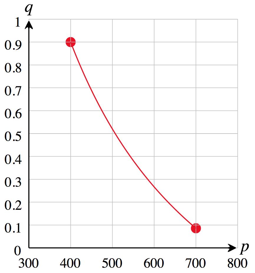
b. 𝑞(400) = 760

So, the change in demand is 0 52 0 9 = 0 38 billion units, which means that demand decreases by about 380 million units sold per year.

Solutions Section 1.2

c. The value of 𝑞 on the graph decreases by smaller and smaller amounts as we move to the right on the graph, indicating that the demand decreases at a smaller and smaller rate (Choice (D)).

30. a. To graph the demand function we use technology with the formula 350/x+0.5 and with xMin = 100 and xMax = 300. Graph:

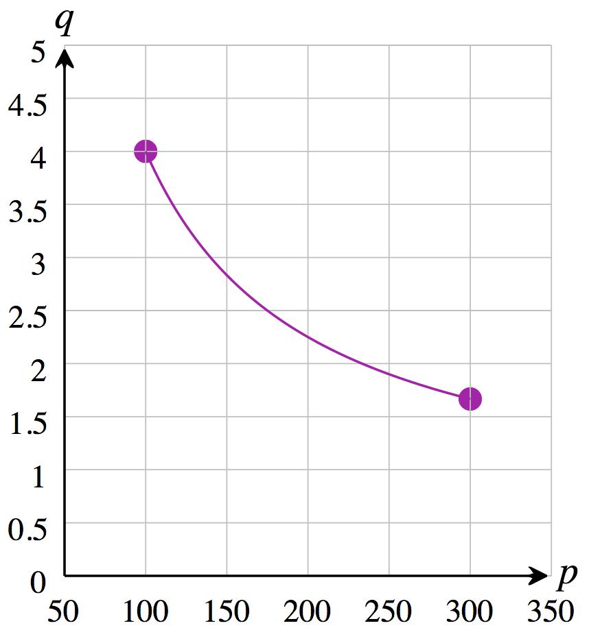
b. 𝑞(100) = 350 100 + 0 5 = 4, 𝑞(200) = 350 200 + 0 5 = 2 25

So, the change in demand is 2.25 4 = 1.75 billion units, which means that demand decreases by about 1.75 billion units sold per year.

c. The value of 𝑞 on the graph increases by larger and larger amounts as we move to the left on the graph, indicating that the demand increases at a greater and greater rate (Choice (A)).

31. The price at which there is neither a shortage nor surplus is the equilibrium price, which occurs when demand = supply:

3𝑝 + 700 = 2𝑝 500

5𝑝 = 1200

𝑝 = $240 per skateboard

32. The price at which there is neither a shortage nor surplus is the equilibrium price, which occurs when demand = supply:

5𝑝 + 50 = 3𝑝 30

8𝑝 = 80

𝑝 = $10 per skateboard

33. a. The equilibrium price occurs when demand = supply:

𝑝 + 57 = 4𝑝 136

5𝑝 = 193

𝑝 = 38 6, or $38,600 per vehicle.

b. Since $38,400 is below the equilibrium price, there would be a shortage at that price. To calculate it, compute demand and supply:

Demand: 𝑞 = 38 4 + 57 = 18 6 million vehicles

Supply: 𝑞 = 4(38 4) 136 = 17 6 million vehicles

Shortage = Demand Supply = 18.6 17.6 = 1 million vehicles

34. a. The equilibrium price occurs when demand = supply:

0 15𝑝 + 23 = 3 85𝑝 131

4𝑝 = 154

𝑝 = 38.5, or $38,500 per vehicle.

b. Since $38,600 is above the equilibrium price, there would be a surplus at that price. To calculate it, compute demand and supply:

Demand: 𝑞 = 0.15(38.6) + 23 = 17.21 million vehicles

Solutions Section 1.2

Supply: 𝑞 = 3 85(38 6) 131 = 17 61 million vehicles

Surplus = Supply Demand = 17.61 17.21 = 0.4 million vehicles

35. a. For equilibrium, Demand = Supply:

760

𝑝 1 = 0.00304𝑝 1

760 𝑝 = 0.0.00304𝑝

Cross-multiply:

0.00304𝑝 2 = 760 ⇒ 𝑝 2 = 760 0 00304 = 250,000

So 𝑝 = 250,000√ = $500

Thus, the equilibrium price is $500, and the equilibrium demand (or supply) is 760∕500 1 = 0 52 billion phones

b. Graph:

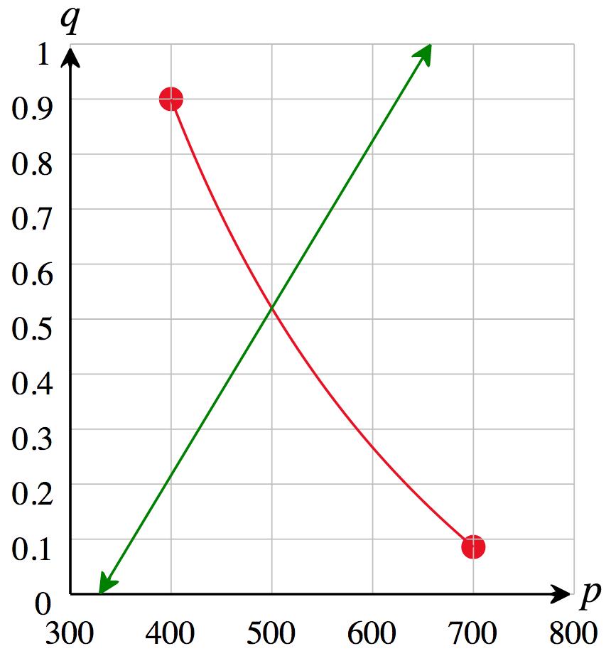
Technology formulas:

Demand: y = 760/x-1

Supply: y = 0.00304x-1

The graphs cross at (500, 0.52) confirming the calclation in part (a).

c. Since $400 is below the equilibrium price, there would be a shortage at that price. To calculate it, compute demand and supply: Demand: 𝑞 = 760 400 1 = 0.9 billion phones

Supply: 0 00304(400) 1 = 0 216 billion phones

Shortage = Demand Supply ≈ 0.9 0.216 = 0.684 billion phones, or 684 million phones.

36. a. For equilibrium, Demand = Supply:

350

𝑝 + 0.5 = 0.0056𝑝 + 0.5

350

𝑝 = 0.0056𝑝

Cross-multiply:

0.0056𝑝 2 = 350 ⇒ 𝑝 2 = 350 0 0056 = 62,500

So 𝑝 = 62,500√ = $250

Thus, the equilibrium price is $250, and the equilibrium demand (or supply) is 350∕250 + 0 5 = 1 9 billion phones

b. Graph:

Technology formulas:

Demand: y = 350/x+0.5

Supply: y = 0.0056x+0.5

The graphs cross at (250, 1 9) confirming the calclation in part (a).

c. Since $200 is below the equilibrium price, there would be a shortage at that price. To calculate it, compute demand and supply:

Demand: 𝑞 = 350 200 + 0 5 = 2 25 billion phones

Supply: 0.0056(200) + 0.5 = 1.62 billion phones

Shortage = Demand Supply ≈ 2 25 1 62 = 0 63 billion phones, or 630 million phones.

37. 𝐶 (𝑞) = 2,000 + 100𝑞 2

a. 𝐶 (10) = 2,000 + 100(10) 2 = 2,000 + 10,000 = $12,000

b. 𝑁 = 𝐶 𝑆, so 𝑁 (𝑞) = 𝐶 (𝑞) 𝑆(𝑞) = 2,000 + 100𝑞 2 500𝑞

This is the cost of removing 𝑞 lb of PCPs per day after the subsidy is taken into account.

c. 𝑁 (20) = 2,000 + 100(20) 2 500(20) = 2,000 + 40,000 10,000 = $32,000

38. 𝐶 (𝑞) = 1,000 + 100√𝑞

a. 𝐶 (100) = 1,000 + 100 100√ = 1,000 + 100(10) = $2,000

b. 𝑁 = 𝐶 𝑆, so 𝑁 (𝑞) = 𝐶 (𝑞) 𝑆(𝑞) = 1,000 + 100√𝑞 200𝑞

This is the cost for dental coverage to the company if it has 𝑞 employees, after the subsidy is taken into account.

c. 𝑁 (100) = 1,000 + 100 100√ 200(100) = 1000 + 100(10) 20,000 = $18,000

The company makes $18,000 from the government for dental coverage if it employs 100 people.

39. The technology formulas are:

(A) -0.2*t^2+t+16

(B) 0.2*t^2+t+16

(C) t+16

The following table shows the values predicted by the three models:

16 18 20 22 23

As shown in the table, the values predicted by model (B) are much closer to the observed values 𝑆(𝑡) than those predicted by the other models.

b. Since 1998 corresponds to 𝑡 = 8,

𝑆(𝑡) = 0 2𝑡 2 + 𝑡 + 16

𝑆(8) = 0.2(8) 2 + 8 + 16 = 36.8

So the spending on corrections in 1998 was predicted to be approximately $37 billion.

40. The technology formulas are:

(A) 16+2*t

(B) 16+t+0.5*t^2

(C) 16+t-0.5*t^2

The following table shows the values predicted by the three models:

𝑡 0 2 4 6 7

𝑆(𝑡) 16 18 22 28 30 (A) 16 20 24 28 30 (B) 16 20 28 40 47.5 (C) 16 16 12 4 -1.5

As shown in the table, the values predicted by model (A) are much closer to the observed values 𝑆(𝑡) than those predicted by the other models.

b. Since 1998 corresponds to 𝑡 = 8,

𝑆(𝑡) = 16 + 2𝑡

𝑆(8) = 16 + 2(8) = 32

So the spending on corrections in 1998 was predicted to be $32 billion.

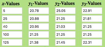
41. The technology formulas are:

(A) 0.005*x+20.75

(B) 0.01*x+20+25/x

(C) 0.0005*x^2-0.07*x+23.25

(The stars are optional for some technologies like graphing calculators and the Evaluator and Grapher App)

Here is result from the Evaluator and Grapher App:

Functions box (Cartesian mode): Evaluator box (Set to 2 decimal places):

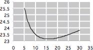
Model (C) fits the data perfectly to two decimal places—more closely than any of the other models. 𝑡 0 2 4 6 7 𝑆(𝑡) 16 18 22 28 30

b. Graph of model (C):

0.0005*x^2-0.07*x+23.25

The lowest point on the graph occurs at 𝑥 = 70 with a 𝑦-coordinate of 20.8. Thus, the lowest cost per shirt is $20.80, which the team can obtain by buying 70 shirts.

42. The technology formulas are:

(A) 0.05*x+20.75

(B) 0.1*x+20+25/x

(C) 0.0008*x^2-0.07*x+23.25

(The stars are optional for some technologies like graphing calculators and the Evaluator and Grapher App)

Here is result from the Evaluator and Grapher App:

Functions box (Cartesian mode): Evaluator box (Set to 2 decimal places):

Model (B) fits the data perfectly to two decimal places—more closely than any of the other models.

b. Graph of model (B):

0.1*x+20+25/x

The lowest point on the graph occurs at 𝑥 = 16 with a y-coordinate of 23.1625. Thus, the lowest cost per hat is $23.16, which the team can obtain by buying 16 hats.

43. Here are the technology formulas as entered in the online Function Evaluator and Grapher at the Web Site:

(A) 0.075*0.83^x

(B) 0.24/(x+3)

(C) 0.00054*x^2-0.012*x+0.075

(D) -0.006*x+0.065

The following graph shows all four curves together with the plotted points (entered as shown in the margin technology note with Example 5).

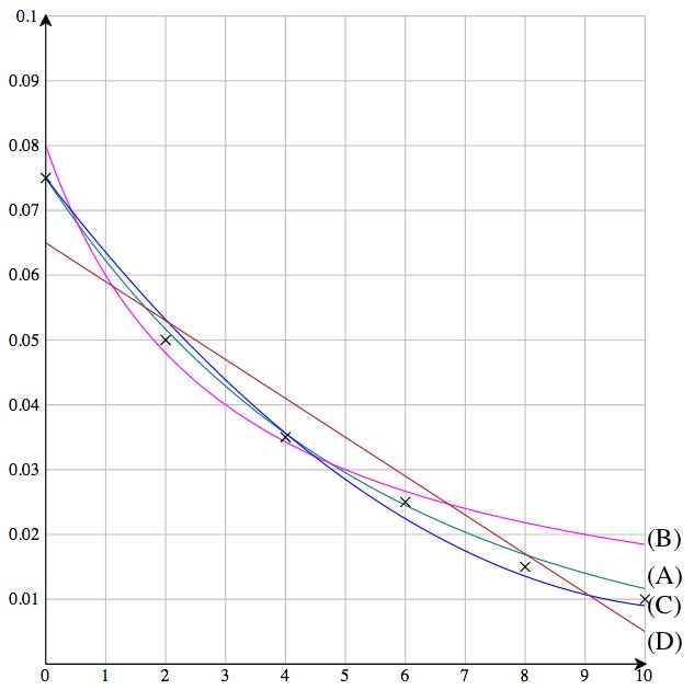
As shown in the graph, the values predicted by models (A) and (C) are much closer to the observed values than those predicted by the other models.

b. Since 2030 corresponds to 𝑡 = 20,

Model (A): 𝑐(20) = 0.075 * 0.83 20 ≈ $0.00181

Model (C): 𝑐(20) = 0 00054(20 2) 0 012(20) + 0 075 ≈ $0 0510

So model (A) gives the lower price: approximately $0.0018 per GB.

44. Here are the technology formulas as entered in the online Function Evaluator and Grapher at the Web Site:

(A) -0.038+0.8/(x+7)

(B) 0.075*1.21^(-x)

(C) 0.00034*(x-14.5)^2

(D) -0.022+0.8/(x+9.32)

The following graph shows all three curves together with the plotted points (entered as shown in the margin technology note with Example 5).

As shown in the graph, the values predicted by models (A), (B), and (C) are much closer to the observed values than those predicted by (D).

b. Since 2030 corresponds to 𝑡 = 20,

Model (A): 𝑐(20) = 0.038 + 0 8 20 + 7 ≈ $0.084 (unreasonable as prices cannot be negative)

Model (B): 𝑐(20) = 0 075(1 21 20) ≈ $0 0017 (reasonable given the current trends)

Model (C): 𝑐(20) = 0 00034(20 14 5) 2 ≈ $0 010 (unreasonable that the price would be the same again in 10 years)

45. A plot of the given points gives a straight line (Option (A)). Options (B) and (C) give curves, so (A) is the best choice.

46. Plotting the three data points suggests a concave down curve, suggesting that a linear model may not be the best fit. An exponential model 𝑝(𝑡) = 𝐴𝑏 𝑡 would result in a concave up curve, regardless of whether 𝑏 is larger than 1 or less than 1. This leaves a quadratic model as the only possible choice. In fact, a quadratic can always be found that passes through any three points not on the same straight line with different 𝑥-coordinates. Therefore, a quadratic model would give an exact fit.

47. A plot of the given data suggests a concave-down curve that becomes steeper downward as the price 𝑝 increases, suggesting Model (D). Model (A) would predict increasing demand with increasing price, Model (B) would correspond to a descending curve that becomes less steep as 𝑝 increases (a concave up curve), and Model (C) would give a concave-up parabola.

48. Model (B) is the best choice; Model (A) would predict increasing demand with increasing price, Model (D) would correspond to a concave down parabola, and Model (C), would predict demand that, rather than flattening out as the price increases, would begin to climb again.

49. Apply the formula

𝐴(𝑡) = 𝑃 !1 + 𝑟 𝑛 " 𝑛𝑡 with 𝑃 = $1,000, 𝑟 = 6∕100 = 0 06, 𝑛 = 4, 𝑡 = 4

𝐴(4) = 1,000(1 + 0 06 4 ) 4×4 = 1,000(1 015) 16 ≈ $1,268 99

50. Apply the formula

𝐴(𝑡) = 𝑃 !1 + 𝑟 𝑛 " 𝑛𝑡 with 𝑃 = $10,000, 𝑟 = 2∕100 = 0.02, 𝑛 = 4, 𝑡 = 5

𝐴(5) = 1,000(1 + 0.02 4 ) 4×5 = 1,000(1.005) 20 ≈ $11,048.96

51. Apply the formula

𝐴(𝑡) = 𝑃 !1 + 𝑟 𝑛 " 𝑛𝑡 with 𝑃 = 5,000, 𝑟 = 0.15∕100 = 0.0015, and 𝑛 = 12. We get the model

𝐴(𝑡) = 5,000(1 + 0 0015∕12) 12𝑡

In June 2028 (𝑡 = 7), the deposit would be worth 5,000(1 + 0.0015∕12) 12(7) ≈ $5,053.

52. Apply the formula

𝐴(𝑡) = 𝑃 !1 + 𝑟 𝑛 " 𝑛𝑡 with 𝑃 = 4,000, 𝑟 = 0.0120, and 𝑛 = 365. We get the model

𝐴(𝑡) = 4,000(1 + 0 0120∕365) 365𝑡

In March 2029 (𝑡 = 8), the deposit would be worth 4,000(1 + 0.0120∕365) 365(8) ≈ $4,403.

53. 𝑃 (0) = 200, 𝑃 (1) = 230, 𝑃 (2) = 260, and so on. Thus, the population is increasing by 30 per year.

54. 𝐵(0) = 5000, 𝐵(1) = 4800, 𝐵(2) = 4600, and so on. Thus, the balance is decreasing by $200 per day.

55. Curve fitting. The model is based on fitting a curve to a given set of observed data.

56. Analytical. The model is obtained by analyzing the situation being modeled.

57. The given model is 𝑐(𝑡) = 4 0 2𝑡 This tells us that 𝑐 is $4 at time 𝑡 = 0 (January) and is decreasing by $0.20 per month. So, the cost of downloading a movie was $4 in January and is decreasing by 20¢ per month.

58. The given model is 𝑐(𝑡) = 4 0.2𝑡 and therefore passes through the points (𝑡, 𝑐) = (0, 4) and (1, 3.8). So, the cost of downloading a movie was $4 in January and $3.80 in February.

59. In a linear cost function, the variable cost is 𝑥 times the marginal cost.

60. In a linear cost function, the marginal cost is the additional (or incremental) cost per item.

61. Yes, as long as the supply is going up at a faster rate, as illustrated by the following graph:

62. There would be a shortage at any given price. Therefore, consumers would be willing to pay more for a scarce commodity and sellers would naturally oblige by charging more, resulting in an upward spiral of prices for the commodity.

63. Extrapolate both models and choose the one that gives the most reasonable predictions.

64. No; as long as 𝑎 is negative, the value of 𝑠(𝑡) for large 𝑡 will be negative, making the model unreasonable for large value of 𝑡.

65. The value of 𝑓 𝑔 at 𝑥 is 𝑓 (𝑥) 𝑔(𝑥) Since 𝑓 (𝑥) ≥ 𝑔(𝑥) for every 𝑥, it follows that 𝑓 (𝑥) 𝑔(𝑥) ≥ 0 for every 𝑥.

66. The value of 𝑓 𝑔 at 𝑥 is 𝑓 (𝑥) 𝑔(𝑥) Since 𝑓 (𝑥) > 𝑔(𝑥) > 0 for every 𝑥, it follows that 𝑓 (𝑥) 𝑔(𝑥) > 1 for every 𝑥

67. Since the values of 𝑓 𝑔 at 𝑥 are ratios 𝑓 (𝑥) 𝑔(𝑥) , it follows that the units of measurement of 𝑓 𝑔 are units of 𝑓 per unit of 𝑔; that is, books per person.

68. Write 𝑓 (𝑥) = 𝑚𝑥 + 𝑏 and 𝑔(𝑥) = 𝑛𝑥 + 𝑐. Then 𝑓 (𝑥) 𝑔(

), also a linear function.

Section 1.3

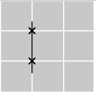
1.

We calculate the slope 𝑚 first. The first two points shown give changes in 𝑥 and 𝑦 of

Δ𝑥 = 0 ( 1) = 1

Δ𝑦 = 8 5 = 3 This gives a slope of

𝑚 = Δ𝑦

Δ𝑥 = 3 1 = 3.

Now look at the second and third points: The change in 𝑥 is again

Δ𝑥 = 1 0 = 1 and so Δ𝑦 must be given by the formula

Δ𝑦 = 𝑚Δ𝑥

Δ𝑦 = 3(1) = 3

This means that the missing value of 𝑦 is 8 + Δ𝑦 = 8 + 3 = 11

𝑥 1 0 1 𝑦 5 8 𝑥 1 0 1 𝑦 1 3

2. We calculate the slope 𝑚 first. The first two points shown give changes in 𝑥 and 𝑦 of

Δ𝑥 = 0 ( 1) = 1

Δ𝑦 = 3 ( 1) = 2

This gives a slope of

𝑚 = Δ𝑦

Δ𝑥 = 2 1 = 2

Now look at the second and third points: The change in 𝑥 is again

Δ𝑥 = 1 0 = 1 and so Δ𝑦 must be given by the formula

Δ𝑦 = 𝑚Δ𝑥

Δ𝑦 = 2(1) = 2

This means that the missing value of 𝑦 is 3 + Δ𝑦 = 3 + ( 2) = 5.

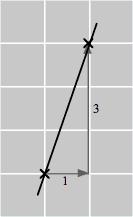
3. We calculate the slope 𝑚 first. The first two points shown give changes in 𝑥 and 𝑦 of

𝑥 2 3 5

𝑦 1 2

Δ𝑥 = 3 2 = 1

Δ𝑦 = 2 ( 1) = 1

This gives a slope of 𝑚 = Δ𝑦

Δ𝑥 = 1 1 = 1.

Now look at the second and third points: The change in 𝑥 is

Δ𝑥 = 5 3 = 2 and so Δ𝑦 must be given by the formula

Δ𝑦 = 𝑚Δ𝑥

Δ𝑦 = ( 1)(2) = 2

This means that the missing value of 𝑦 is 2 + Δ𝑦 = 2 + ( 2) = 4

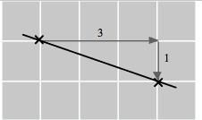
𝑥 2 4 5

𝑦 1 2

We calculate the slope 𝑚 first. The first two points shown give changes in 𝑥 and 𝑦 of

Δ𝑥 = 4 2 = 2

Δ𝑦 = 2 ( 1) = 1

This gives a slope of

𝑚 = Δ𝑦

Δ𝑥 = 1 2 = 1 2 .

Now look at the second and third points: The change in 𝑥 is

Δ𝑥 = 5 4 = 1 and so Δ𝑦 must be given by the formula

Δ𝑦 = 𝑚Δ𝑥

Δ𝑦 = ! 1 2 "(1) = 1 2

This means that the missing value of 𝑦 is 2 + Δ𝑦 = 2 + ! 1 2 " = 5 2 or 2 5

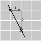
5. We calculate the slope 𝑚 first. The first and third points shown give changes in 𝑥 and 𝑦 of

𝑥 2 0 2

𝑦 4 10

Δ𝑥 = 2 ( 2) = 4

Δ𝑦 = 10 4 = 6

This gives a slope of

𝑚 = Δ𝑦

Δ𝑥 = 6 4 = 3 2 .

Now look at the first and second points: The change in 𝑥 is

Δ𝑥 = 0 ( 2) = 2 and so Δ𝑦 must be given by the formula

Δ𝑦 = 𝑚Δ𝑥

Δ𝑦 = ! 3 2 "(2) = 3

This means that the missing value of 𝑦 is 4 + Δ𝑦 = 4 + 3 = 7.

6. We calculate the slope 𝑚 first. The first and third points shown give changes in 𝑥 and 𝑦 of

𝑥 0 3 6

𝑦 1 5

Δ𝑥 = 6 0 = 6

Δ𝑦 = 5 ( 1) = 4

This gives a slope of 𝑚 = Δ𝑦

Δ𝑥 = 4 6 = 2 3 .

Now look at the first and second points: The change in 𝑥 is

Δ𝑥 = 3 0 = 3 and so Δ𝑦 must be given by the formula

Δ𝑦 = 𝑚Δ𝑥

Δ𝑦 = ! 2 3 "(3) = 2

This means that the missing value of 𝑦 is 1 + Δ𝑦 = 1 + ( 2) = 3

7. From the table, 𝑏 = 𝑓 (0) = 2

The slope (using the first two points) is

Thus, the linear equation is

8. From the table, 𝑏 = 𝑓 (0) = 3.

The slope (using the first two points) is

Thus, the linear equation is

9. The slope (using the first two points) is

To obtain 𝑓 (0) = 𝑏, use the formula for 𝑏 :

(0) = 𝑏 = 𝑦1 𝑚𝑥1 = 1 ( 1)( 4) = 5

This gives 𝑓 (𝑥) = 𝑚𝑥 + 𝑏 = 𝑥 5

10. The slope (using the first two points) is 𝑚 = 𝑦2 𝑦1 𝑥2 𝑥1 = 6 4 2 1 = 2 1 = 2

To obtain 𝑓 (0) = 𝑏, use the formula for 𝑏 : 𝑓 (0) = 𝑏 = 𝑦1 𝑚𝑥1 = 4 (2)(1) = 2

This gives

𝑓 (𝑥) = 𝑚𝑥 + 𝑏 = 2𝑥 + 2

Using the point (𝑥1 , 𝑦1 ) = ( 4, 1)

Using the point (𝑥1 , 𝑦1 ) = (1, 4)

11. In the table, 𝑥 increases in steps of 1 and 𝑓 increases in steps of 4, showing that 𝑓 is linear with slope

𝑚 = Δ𝑦 Δ𝑥 = 4 1 = 4 and intercept

𝑏 = 𝑓 (0) = 6 giving

𝑓 (𝑥) = 𝑚𝑥 + 𝑏 = 4𝑥 + 6

The function 𝑔 does not increase in equal steps, so 𝑔 is not linear.

12. In the table, 𝑥 increases in steps of 10 and 𝑔 increases in steps of 5, showing that 𝑔 is linear with slope

𝑚 = Δ𝑦 Δ𝑥 = 5 10 = 1 2 and intercept

𝑏 = 𝑔(0) = 4 giving

𝑔(𝑥) = 𝑚𝑥 + 𝑏 = 1 2 𝑥 4

Solutions Section 1.3

The function 𝑓 does not increase in equal steps, so 𝑓 is not linear.

13. In the first three points listed in the table, 𝑥 increases in steps of 3, but 𝑓 does not increase in equal steps, whereas 𝑔 increases in steps of 6. Thus, based on the first three points, only 𝑔 could possibly be linear, with slope

𝑚 = Δ𝑦

Δ𝑥 = 6 3 = 2 and intercept

𝑏 = 𝑔(0) = 1 giving

𝑔(𝑥) = 𝑚𝑥 + 𝑏 = 2𝑥 1.

We can now check that the remaining points in the table fit the formula 𝑔(𝑥) = 2𝑥 1, showing that 𝑔 is indeed linear.

14. In the first and last pairs of points listed in the table, 𝑥 increases in steps of 3, but 𝑓 does not increase in equal steps, whereas 𝑔 increases in steps of 9. Thus, based on those points, only 𝑔 could possibly be linear, with slope

𝑚 = Δ𝑦 Δ𝑥 = 9 3 = 3 and intercept

𝑏 = 𝑔(0) = 1 giving

𝑔(𝑥) = 𝑚𝑥 + 𝑏 = 3𝑥 1.

We can now check that the remaining points in the table fit the formula 𝑔(𝑥) = 3𝑥 1, showing that 𝑔 is indeed linear.

15. Slope = coefficient of 𝑥 = 3 2

16. Slope = coefficient of 𝑥 = 2 3

17. Slope = coefficient of 𝑥 = 1 6

18. Write the equation as 𝑦 = 2𝑥 3 + 1 3

Slope = coefficient of 𝑥 = 2 3

19. If we solve for 𝑥 we find that the given equation represents the vertical line 𝑥 = 1∕3, and so its slope is infinite (undefined).

20. 8𝑥 2𝑦 = 1. Solving for 𝑦 : 2𝑦 = 8𝑥 1

𝑦 = 4𝑥 1 2

Slope = coefficient of 𝑥 = 4

21. 3𝑦 + 1 = 0. Solving for 𝑦 : 3𝑦 = 1

𝑦 = 1 3

Solutions Section 1.3

Slope = coefficient of 𝑥 = 0

22. If we solve for 𝑥 we find that the given equation represents the vertical line 𝑥 = 3∕2, and so its slope is infinite (undefined).

23. 4𝑥 + 3𝑦 = 7. Solve for 𝑦 : 3𝑦 = 4𝑥 + 7 𝑦 = 4 3 𝑥 + 7 3

Slope = coefficient of 𝑥 = 4 3

24. 2𝑦 + 3 = 0 Solve for 𝑦 : 2𝑦 = 3 𝑦 = 3 2

Slope = coefficient of 𝑥 = 0

25. 𝑦 = 2𝑥 1

𝑦-intercept = 1, slope = 2

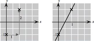
26. 𝑦 = 𝑥 3

𝑦-intercept = 3, slope = 1

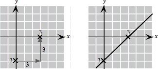
27. 𝑦-intercept = 2, slope = 2 3

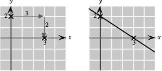
28. 𝑦 = 1 2 𝑥 + 3

𝑦-intercept = 3, slope = 1 2

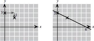
29. 𝑦 + 1 4 𝑥 = 4 Solve for 𝑦 to obtain 𝑦 = 1 4 𝑥 4

y-intercept = 4, slope = 1 4

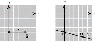
30. 𝑦 1 4 𝑥 = 2 Solve for 𝑦 to obtain 𝑦 = 1 4 𝑥 2

𝑦-intercept = 2, slope = 1 4

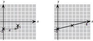
31. 7𝑥 2𝑦 = 7 Solve for 𝑦 : 2𝑦 = 7𝑥 + 7, so 𝑦 = 7 2 𝑥 7 2 𝑦-intercept = 7 2 = 3 5, slope = 7 2 = 3 5

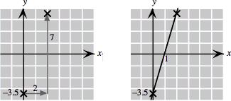
32. 2𝑥 3𝑦 = 1 Solve for 𝑦 : 3𝑦 = 2𝑥 + 1, so 𝑦 = 2 3 𝑥 1 3

𝑦-intercept = 1 3 , slope = 2 3

33. 3𝑥 = 8. Solve for 𝑥 to obtain 𝑥 = 8 3 .

The graph is a vertical line:

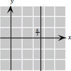
34. 2𝑥 = 7. Solve for 𝑥 to obtain 𝑥 = 7 2 = 3.5.

The graph is a vertical line:

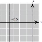
35. 6𝑦 = 9 Solve for 𝑦 to obtain 𝑦 = 9 6 = 3 2 = 1 5

𝑦-intercept = 3 2 = 1 5, slope = 0. The graph is a horizontal line:

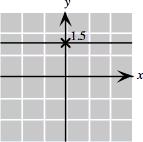
36. 3𝑦 = 4. Solve for 𝑦 to obtain 𝑦 = 4 3

𝑦-intercept = 4 3 , slope = 0. The graph is a horizontal line:

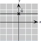
37. 2𝑥 = 3𝑦. Solve for 𝑦 to obtain 𝑦 = 2 3 𝑥

𝑦-intercept = 0, slope = 2 3

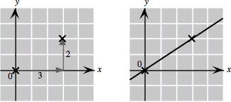
38. 3𝑥 = 2𝑦 Solve for 𝑦 to obtain 𝑦 = 3 2 𝑥

𝑦-intercept = 0, slope = 3 2 39. (0, 0) and (1, 2)

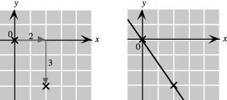
(0, 0) and ( 1, 2)

41. ( 1, 2) and (0, 0)

𝑚 = 𝑦2 𝑦1 𝑥2 𝑥1 = 0 ( 2) 0 ( 1) = 2

43. (4, 3) and (5, 1) 𝑚 =

45. (1, 1) and (1, 2)

47. (2, 3 5) and (4, 6 5) 𝑚

49. (300, 20 2) and (400, 11 2)

𝑚

51. (0, 1) and ! 1 2 , 3 4 " 𝑚 = 𝑦

53. (𝑎, 𝑏) and (𝑐, 𝑑) (𝑎 ≠ 𝑐)

𝑚 = 𝑦2 𝑦1 𝑥2 𝑥1 = 𝑑 𝑏 𝑐 𝑎

55. (𝑎, 𝑏) and (𝑎, 𝑑) (𝑏 ≠ 𝑑)

𝑚 = 𝑦2 𝑦1 𝑥2 𝑥1 = 𝑑 𝑏 𝑎 𝑎 \ \ Undefined

57. ( 𝑎, 𝑏) and (𝑎, 𝑏) (𝑎 ≠ 0) 𝑚 = 𝑦2 𝑦1

42. (2, 1) and (0, 0)

(4, 3) and (4, 1)

and ( 1, 1)

(10, 3 5) and (0, 1 5)

(1, 20 2) and (2, 3 2)

54. (𝑎, 𝑏) and (𝑐, 𝑏) (𝑎 ≠ 𝑐) 𝑚 = 𝑦2 𝑦1 𝑥2 𝑥1 = 𝑏 𝑏 𝑐 𝑎 = 0

56. (𝑎, 𝑏) and ( 𝑎, 𝑏) (𝑎 ≠ 0)

58. (𝑎, 𝑏) and (𝑏, 𝑎) (𝑎 ≠ 𝑏)

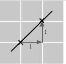
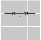
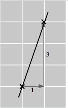
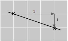
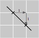
g. Vertical line; undefined slope

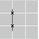
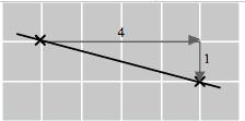
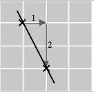
Solutions Section 1.3

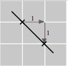
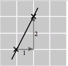
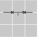
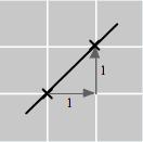
f. Vertical line; undefined slope