Introduction
Montane environments are found in every continent on planet Earth. These areas are important biologically, as clearly portrayed by the Conference of Parties to the United Nations Conventions on Biological Diversity in 2004. The parties posited that montane environments are about the most biologically diverse parts of the Earth. A fact supported by the Conservation International by laying claim to the fact that 25 of the 34 world centers of greatest biodiversity hot spots are wholly or partly mountainous (see Price, 2013). These regions are of rugged terrain and have been defned as areas with an elevation of about 300 m and above over a radius of about 7 km (Wohl, 2018). These regions cover not less than 12% of the earth’s surface and among other things provide various functions such as historical, cultural, religious, and environmental. Historically, these regions have been described as areas where man started domesticating plants and animals. Also, across the world, mountain ranges hold cultural eminence as places of tourist attractions, sports, and home to indigenous people. Montane environments have been deifed across ages and time with various groups of people across the world objectifying mountains and worshiping them. In terms of environment, mountain regions serve as headwater catchment for most of the large rivers of the world (Price et al., 2013). Furthermore, the range of ecosystem services provided by the mountain ecosystem includes, but not limited to, meat, milk, wool, leather, maintenance of atmospheric composition and genetic library, amelioration of water, and conservation of soils (Kang et al., 2018), and it also provides shelter to those living on and around mountain environments. It is a space for social interactions that allow for human-environment interactions. This human-environment interaction allows for the (re)production of goods and services. Due to the physiographic makeup of montane regions, that is, altitude, terrain, soil, and climate, montane environments are hotspots for biodiversity. The variety of plants and animals found within these environments is to a large extent endemic with great genetic diversity. Mountain biota (plants and animals) survive under the environmental conditions of their habitat because of their adaptability, which allows them to establish themselves and reproduce. It is precisely this ability to adapt to the specifc characteristics of a given microsite, which has shaped one of the theories, is what partly explains the endemism found in the mountains through speciation.
From the foregoing, it is clear that montane regions or ecosystems are unique (Semala et al., 2022). Globally, there has been an increase in environmental awareness of various environmental issues. However, within the montane setting, environmental issues such as changing climate, habitat loss and fragmentation, population growth, agricultural activities, and natural hazards are burning issues (Atkinson and De Clercq, 2022; Das and Zhang, 2022, Onaolapo et al., 2022; Luliro et al., 2022). Although these issues are also peculiar to lowland environments, however, because of the physiography of montane environments and the highly sensitive nature of its ecosystems, changes or perturbations create almost irreversible reactions. The changing climate affects snow caps and glaciers on mountain tops by melting these age-long ice caps due to global warming (Boudhar et al., 2022). Also, the slower pace of recovery of natural regenerative processes, owing to colder temperatures, greatly increases potential for erosion, owing to steeper gradients and generally less fertile soil endangers this environment and soil fertility (Adagbasa et al., 2022; Nyawacha and Meta, 2022; Harrison and van Tol, 2022; Luliro et al., 2022). Furthermore, the changing climate is altering habitat makeup of various plants and animals, leading to migration of animals and extinction of some plants, which is a great challenge to the genetic pool of the region (Adagbasa et al., 2022). Besides, changing climate coupled with fres and other anthropogenic activities like overcultivation is leading to loss of carbon stocks in biomass of montane vegetation (Dipuo et al., 2022; Adagbasa et al., 2022; Onaolapo et al., 2022). These issues and many more impact on the livelihoods of mountain people. To the indigenous peoples and those whose livelihoods depend on the ecology of the mountains most often than not see this physical entity, mountain, not just as a natural resource but also as part of their existence (Sharma et al., 2019). To those living within and beyond, they understand that their well-being, to some extent their identity, especially for those living there, depends on careful stewardship of the montane ecosystems (Wang et al., 2019). However, in the light of the changing climate and its direct and indirect consequences, new and emerging socio-economic patterns within and around mountain environments are developing which not only affect those living within and around the mountain but also those whose livelihoods depend on the montane ecosystems. Addressing these issues requires careful planning and the need to understand various aspects of montane environments. As against lowland areas where intensive feld studies can be carried out, montane areas due to their physiography and location limit the number of feld studies that could be carried out. Some mountains are so remote that to understand the dynamics of such environments requires remote sensing through the use of satellites or unmanned aerial vehicles (UAVs) (Semala et al., 2022). Remote sensing, in contrast with traditional approaches, such as feld studies, offers spatial and temporal data that are convenient for mapping large areas at different spatial scales in a more vigorous, rapid, and effcient manner (Fajji, 2015). Globally, we know more about mountain ranges in Asia, North and South America, and Europe than the ones in Africa. Several studies and documentaries abound for the Himalayas, Andes, Alps, etc. (see Smethurst, 2000; Funnell and Price, 2003; Wester et al., 2019). Studies for these ranges increased in light of the changing climates and global warming. Some of these studies focused on sea-level rise, melting ice caps, coastal cities in the global north, and
changing lifestyle for those living around these ranges (Anderson et al., 2020; Jorgenson and Ely, 2001; Wang et al., 2020). However, in Africa, besides the EastAfrican Range (such as Kilimanjaro, Rwenzori), part of the Drakensberg and part of the high Atlas in North Africa (Smethurst, 2000; Thompson et al., 2002; Kaser et al., 2004; Jacobs et al., 2016; Teixell et al., 2003; Sebrier et al., 2006; Büscher, 2012), little is known about other montane environments. As portrayed by Smethurst (2000), little or nothing is known about the mountains in Madagascar, Cape Verde, and other countries. Furthermore, despite the array of information available for some mountain ranges in different parts of the world, global assessments such as the Intergovernmental Panel on Climate Change and the Millennium Ecosystem Assessment provide detailed information as regards mountain environments with respect to scientifc and traditional indigenous knowledge (Wester et al., 2019). Besides, only four journals deal with mountain environments globally (the Journal on Protected Mountain Areas Research, Sustainable Development of Mountain Territories, Mountain Research and Development, and the Journal of Mountain Science). Therefore, this book will open up closed mountain areas of Africa and present new and emerging studies within and around known and unknown mountain ranges in Africa using remote sensing techniques. This will push further the frontier of knowledge in mountain studies and help shape further global assessments and policies. The 11 chapters presented in this book fall within the following thematic areas. These are:
1. Satellite Remote Sensing and Montane Vegetation
2. Satellite Remote Sensing and Mountain Hazards
3. Satellite Remote Sensing and Mountain Ecosystem Services
4. Satellite Remote Sensing of Mountain Geological and Geomorphic Surfaces
5. Satellite Remote Sensing and Mountain Energy Balance Modelling
The fndings presented in this book will drive global policies and help strengthen these fragile ecosystems in Africa. With the impact of climate change already seen in various parts of the continent and especially in Sub-Saharan Africa, this book will help understand the role climate change is playing within mountain systems and the impact on those depending on them for their livelihoods either directly or indirectly. Lastly, even though the studies covered in the book cannot touch every aspect of mountain systems, it is expected that enough would have been presented in the book to help drive policies and establish montane research units across the continent.
References
Adagbasa, G. E., Adelabu, S. A., & Okello, T. W. (2022). Ecological vulnerability assessment to Grassland fres in a protected mountainous area using remote sensing and GIS. In S. Adelabu, R. Abel, A. Olusola, & A. Efosa (Eds.), Remote sensing of African mountains: Geospatial tools toward sustainability. Springer. Anderson, J. T., Wilson, G. S., Jones, R. S., Fink, D., & Fujioka, T. (2020). Ice surface lowering of Skelton Glacier, Transantarctic Mountains, since the Last
Glacial Maximum: Implications for retreat of grounded ice in the western Ross Sea. Quaternary Science Reviews, 237, 106305.
Atkinson, J., & De Clercq, W. (2022). Unravelling regional geodiversity: A gridmapping approach to quantify geodiversity in the Uthukela District, Kwazulunatal. In S. Adelabu, R. Abel, A. Olusola, & A. Efosa (Eds.), Remote sensing of African mountains: Geospatial tools toward sustainability. Springer.
Boudhar, A., Wassim Mohamed Baba, W. M., Marchane, A., Ouatiki, H., Bouamri, H., Hanich, L., & Chehbouni, A. (2022). Water resources monitoring over the Atlas Mountains in Morocco using satellite observations and Reanalysis data. In S. Adelabu, R. Abel, A. Olusola, & A. Efosa (Eds.), Remote sensing of African mountains: Geospatial tools toward sustainability. Springer.
Büscher, B. (2012). Payments for ecosystem services as neoliberal conservation: (Reinterpreting) evidence from the Maloti-Drakensberg, South Africa. Conservation and Society, 10(1), 29–41.
Das, P., & Zhang, Z. (2022). Monitoring the wildfre activity and ecosystem response on Mt. Kilimanjaro using Earth Observation data and GIS. In S. Adelabu, R. Abel, A. Olusola, & A. Efosa (Eds.), Remote sensing of African mountains: Geospatial tools toward sustainability. Springer.
Dipuo, O. M., Olusola, A., & Adewale, S. A. (2022). Development of lightning hazard map for fre danger assessment over Mountainous Protected Area using geospatial technology. In S. Adelabu, R. Abel, A. Olusola, & A. Efosa (Eds.), Remote sensing of African mountains: Geospatial tools toward sustainability Springer.
Fajji, N. G. (2015). A remote sensing and GIS scheme for rangeland quality assessment and management in the North-West Province, South Africa [Doctoral dissertation]. North-West University, South Africa.
Funnell, D. C., & Price, M. F. (2003). Mountain geography: A review. The Geographical Journal, 169(3), 183–190.
Harrison, R., & van Tol, J. (2022). Digital Soil Mapping for hydropedological purposes of the Cathedral Peak research catchments, South Africa. In S. Adelabu, R. Abel, A. Olusola, & A. Efosa (Eds.), Remote sensing of African mountains: Geospatial tools toward sustainability. Springer.
Jacobs, L., Dewitte, O., Poesen, J., Delvaux, D., Thiery, W., & Kervyn, M. (2016). The Rwenzori Mountains, a landslide-prone region? Landslides, 13(3), 519–536.
Jorgenson, T., & Ely, C. (2001). Topography and fooding of coastal ecosystems on the Yukon-Kuskokwim Delta, Alaska: Implications for sea-level rise. Journal of Coastal Research, 124–136.
Kang, P., Chen, W., Hou, Y., & Li, Y. (2018). Linking ecosystem services and ecosystem health to ecological risk assessment: A case study of the Beijing-TianjinHebei urban agglomeration. Science of the Total Environment, 636, 1442–1454. Kaser, G., Hardy, D. R., Mölg, T., Bradley, R. S., & Hyera, T. M. (2004). Modern glacier retreat on Kilimanjaro as evidence of climate change: observations and facts. International Journal of Climatology: A Journal of the Royal Meteorological Society, 24(3), 329–339.
Luliro, N. D., Dbumba, D. S., Nammanda, I., & Kisira, Y. (2022). Effect of climate variability and change on land suitability for Irish Potato Production in Kigezi
Highlands of Uganda. In S. Adelabu, R. Abel, A. Olusola, & A. Efosa (Eds.), Remote sensing of African mountains: Geospatial tools toward sustainability. Springer.
Nyawacha, S. O., & Meta, V. K. (2022). Assessing the vulnerability of the Eastern Africa Highlands’ soils to rainfall erosivity. In S. Adelabu, R. Abel, A. Olusola, & A. Efosa (Eds.), Remote sensing of African mountains: Geospatial tools toward sustainability. Springer.
Onaolapo, T. F., Okello, T. W., & Adelabu, S. A. (2022). Evaluating settlement development change, pre, and post-1994 in the Drakensberg mountains of Afromontane region, South Africa. In S. Adelabu, R. Abel, A. Olusola, & A. Efosa (Eds.), Remote sensing of African mountains: Geospatial tools toward sustainability. Springer.
Price, M. F. (2013). Mountain geography: Physical and human dimensions University of California Press.
Price, M. F., & Kohler, T. (2013). Sustainable mountain development. In M. F. Price, A. C. Byers, D. A. Friend, T. Kohler, & L. W. Price (Eds.), Mountain geography (pp. 333–365). University of California Press.
Sébrier, M., Siame, L., Zouine, E. M., Winter, T., Missenard, Y., & Leturmy, P. (2006). Active tectonics in the moroccan high atlas. Comptes Rendus Geoscience, 338(1–2), 65–79.
Semala, M., Olusola, A., Adelabu, S., & Ramoelo, A. (2022). Montane grasslands: Biomass estimations using remote sensing techniques in Africa. In S. Adelabu, R. Abel, A. Olusola, & A. Efosa (Eds.), Remote sensing of African mountains: Geospatial tools toward sustainability. Springer.
Sharma, E., Molden, D., Rahman, A., Khatiwada, Y. R., Zhang, L., Singh, S. P., … & Wester, P. (2019). Introduction to the hindu kush himalaya assessment. In The Hindu Kush Himalaya Assessment (pp. 1–16). Springer.
Smethurst, D. (2000). Mountain geography. Geographical Review, 90(1), 35–56
Teixell, A., Arboleya, M. L., Julivert, M., & Charroud, M. (2003). Tectonic shortening and topography in the central High Atlas (Morocco). Tectonics, 22(5).
Thompson, L. G., Mosley-Thompson, E., Davis, M. E., Henderson, K. A., Brecher, H. H., Zagorodnov, V. S., … & Beer, J. (2002). Kilimanjaro ice core records: evidence of Holocene climate change in tropical Africa. Science, 298(5593), 589–593.
Wang, Y., Wu, N., Kunze, C., Long, R., & Perlik, M. (2019). Drivers of change to mountain sustainability in the Hindu Kush Himalaya. In The Hindu Kush Himalaya Assessment (pp. 17–56). Springer.
Wang, Y., Zhang, T., Xiao, C., Ren, J., & Wang, Y. (2020). A two-dimensional, higher-order, enthalpy-based thermomechanical ice fow model for mountain glaciers and its benchmark experiments. Computers & Geosciences, 104526. Wester, P., Mishra, A., Mukherji, A., & Shrestha, A. B. (2019). The Hindu Kush Himalaya assessment: Mountains, climate change, sustainability and people (p. 627). Springer Nature.
Wohl, E. (2018). Mountain environments. obo in environmental science. https://doi. org/10.1093/obo/9780199363445-0094
1 Montane Grasslands: Biomass Estimations Using Remote Sensing Techniques in Africa . .
Semala Mathapelo, Adeyemi Olusola, Samuel Adelabu, and Abel Ramoelo
2 Unravelling Regional Geodiversity: A Grid-Mapping Approach to Quantify Geodiversity in the uThukela District, KwaZulu-Natal .
Jonathan T. Atkinson and Willem P. De Clercq
3 Monitoring the Wildfire Activity and Ecosystem Response on Mt. Kilimanjaro Using Earth Observation Data and GIS . . .
Priyanko Das, Zhenke Zhang, and Hang Ren
4 Ecological Vulnerability Assessment to Grassland Fires in a Protected Mountainous Area Using Remote Sensing and GIS .
E. Adagbasa, Samuel Adelabu, and T. W. Okello
1
19
. 51
5 Natural Hazards Magnitude, Vulnerability, and Recovery Strategies in the Rwenzori Mountains, Southwestern Uganda . . . . . 83 Bernard Barasa, Bob Nakileza, Frank Mugagga, Denis Nseka, Hosea Opedes, Paul Makoba Gudoyi, and Benard Ssentongo
6 Assessing the Vulnerability of the Eastern Africa Highlands’ Soils to Rainfall Erosivity
Seth O. Nyawacha and Viviane K. Meta
7 Development of Lightning Hazard Map for Fire Danger Assessment Over Mountainous Protected Area Using Geospatial Technology
Dipuo Olga Mofokeng, Adeyemi Olusola, and Samuel Adelabu
8 Water Resources Monitoring Over the Atlas Mountains in Morocco Using Satellite Observations and Reanalysis Data . . . . . 157
Abdelghani Boudhar, Wassim Mohamed Baba, Ahmed Marchane, Hamza Ouatiki, Hafsa Bouamri, Lahoucine Hanich, and Abdelghani Chehbouni
9 Evaluating Settlement Development Change, Pre, and Post-1994 in the Drakensberg Mountains of Afromontane Region, South Africa
T. F. Onaolapo, T. W. Okello, and S. A. Adelabu
10 Digital Soil Mapping for Hydropedological Purposes of the Cathedral Peak Research Catchments, South Africa . .
193 Rowena Harrison and Johan van Tol
11 Effect of Climate Variability and Change on Land Suitability for Irish Potato Production in Kigezi Highlands of Uganda 215 Nadhomi Daniel Luliro, Daniel Saul Ddumba, Irene Nammanda, and Yeeko Kisira
List of Figures
Fig. 1.1 Flowchart showing the methodology and outputs
Fig. 1.2 Thematic evolution describing the focus of studies from 2003 to 2020
Fig. 1.3 Three-feld plot showing keywords (left), authors (middle) and keyword plus (right) .
Fig. 2.1 (a) Map showing the uThukela District Municipality (UTDM) situated in the western region of KwaZulu-Natal, South Africa (DEM Source: CGIAR, 2014). (b) The conceptual workfow uses gridded datasets to derive geodiversity sub-index data layers for the UTDM region overlaid with the 2.5 × 2.5 km sample grid
Fig. 2.2
Fig. 2.3
Concept of the geodiversity quantifcation of vector datasets in the 2.5 × 2.5 km grid. (a) Overview map showing vector soil association(s) in a 3 × 3 window range. (b) Counting the number of soil forms per grid cell is too conservative with only three soil form features counted and full abundance of soil features not quantifed. (c) Counting the number of vector features per grid cell is too liberal with a total of 9 soil form features counted. Duplication of similar features resulting in an overestimation of geodiversity per grid cell. (d) Counting the number of vector features per network cell per spatially contiguous element.: “Goldilocks case” of quantifying vector feature diversity resulting in four soil form features per grid . . . . 32
Concept of the geodiversity quantifcation of raster datasets in the 2.5 × 2.5 km grid. (a) SRTM 90 m elevation for two grid cells (a1) having an elevation height range of 413 m and (a2) having an elevation height range of 345 m. Grids highlighted in (b1) and (b2) have been generalised using the Zonal Statistical modal value for elevation calculated for each grid cell resulting in new elevation grid values of 375 m and 305 m, respectively, for the geodiversity index calculation .
32
Fig. 2.4 Calculation of geodiversity index applied to UTDM as the sum of seven sub-indices: Hi, Pi, Li, Ci, Ti, Gi and Si. The fnal thematic geodiversity layer is interpolated using a geostatistical interpolation approach to provide a smooth surface of diversity and rescaled and classifed to a fve-class scale of theoretical geodiversity index. (a) Hydrographic diversity index. (b) Lithographic diversity index. (c) Pedological diversity index. (d) Climatic diversity index. (e) Topographic diversity index. (f) Geomorphometric diversity index. (g) Solar morphometric diversity index. (h) GDIx grid. (i) Modelled GDIx
Fig. 3.1 Location map of Mt. Kilimanjaro .
Fig. 3.2 Spectral refectance curve for comparison of healthy vegetation and burned areas. (Source: US Forest service)
Fig. 3.3 Mt. Kilimanjaro Forest fre 11 October 2020. (a) MODIS burnt area and Julian days detected by MCD64A1 during 01 October 2020 to 31 October 2020 and true color composite Sentinel-2 image on 17 August 2017. (b) dNBR (difference normalized burn ratio) for burn severity classes during 08 October 2020 to 15 October 2020 and true color composite Sentinel-2 image on 17 August 2017. (c) Monitoring burn area after the post-fre event by BAIS2 (burn area index from Sentinel-2) on 15 October 2020
Fig. 3.4 Eight-day composite of LAI at Mt. Kilimanjaro. (a) Before fre (22–30 September 2020). (b) After fre event (8–15 October 2020) and burn area retrieved from MODIS (MCD64A1)
Fig. 3.5 Eight-day composite of NDVI at Mt. Kilimanjaro. (a) Before fre (22–30 September 2020). (b) After fre event (8–15 October 2020) and burn area retrieved from MODIS (MCD64A1)
37
54
58
59
60
61
Fig. 3.6 Correlation between burn area index (BAIS2) and vegetation indices (VIs). (a) NDVI vs BAIS2. (b) LAI vs BAIS2 during 1 September 2020–10 February 2020 62
Fig. 3.7 Mt. Kilimanjaro Leaf Area Index LAI trend from 7 October 2020 to 2 February 2021 63
Fig. 4.1 Study area.
Fig. 4.2 Ecological vulnerability model
Fig. 4.3 Spatial distribution of S. plumosum and E. curvula extracted from vegetation species map (Adagbasa et al., 2019)
Fig. 4.4 Ecological vulnerability to fre.
Fig. 4.5 (a) Correlation between S. plumosum and ecological vulnerability. (b) Correlation between E. curvula and ecological vulnerability. The value on the Y-axis presents the vulnerability categories. 1.0 represents low vulnerability, 2.0 medium, and 3.0 high vulnerability. The X-axis represents the species abundance. .
Fig. 5.1 Location of Mountain Rwenzori in Uganda
Fig. 5.2 Natural hazards experienced in Mountain Rwenzori .
Fig. 5.3 Elements at risk in Mountain Rwenzori.
Fig. 5.4
91
93
Elements that are vulnerable to drought hazard in Mt. Rwenzori .
Fig. 5.5 Elements that are vulnerable to earthquake hazard in Mt. Rwenzori 95
Fig. 5.6 Elements that are vulnerable to food hazard in Mt. Rwenzori 96
Fig. 5.7 Croplands that are vulnerable to hailstorm hazard in Mt. Rwenzori 97
Fig. 5.8 Elements that are vulnerable to landslide hazard in Mt. Rwenzori 98
Fig. 5.9 Elements that are vulnerable to lightning hazard in Mt. Rwenzori 99
Fig. 5.10 Elements that are vulnerable to windstorm hazard in Mt. Rwenzori 100
Fig. 6.1 Altitude map of the eastern Africa region, with an emphasis on the areas with high elevation 121
Fig. 6.2 Rainfall erosivity in the Eastern Africa
123
Fig. 6.3 Soil erodibility in the Eastern Africa Area in 2020 124
Fig. 6.4 C factor in the Eastern Africa region 125
Fig. 6.5 The management conservation practices in the Eastern Africa region 126
Fig. 6.6 Water erosion risk areas in the Eastern Africa in 2020 127
Fig. 6.7 Graph showing the statistics distribution of risk areas to water erosion in Eastern Africa 128
Fig. 7.1 Location of the study area (GGHNP) 134
Fig. 7.2 Map depicting the spatial density of CG lightning fashes within GGHNP between 2007 and 2018. Lightning density (Ng) displayed the number of CG lightning events per km2 per year
Fig. 7.3 Graph of lightning events by year and hour
Fig. 7.4 Seasonal variation lightning strikes over GGHNP. .
Fig. 7.5 Global Moran I statistic results for monthly data (a) Moran I vs Distance, (b) Z-score vs Distance
Fig. 7.6 Global Moran I statistic diurnal data (a) Moran I vs Distance, (b) Z-score vs Distance
Fig. 7.7 GGHNP lightning strike density showing hot and cold spots . . . .
Fig. 7.8 GGHNP monthly lightning strike density showing hot and cold spots.
Fig. 7.9 GGHNP average hourly lightning strike density showing hot and cold spots.
Fig. 7.10 GGHNP average hourly lightning strike density showing hot and cold spots (contd)
Fig. 7.11 Lightning hazard map for GGHNP (2007–2017) showing coverage extent of hazard severity
Fig. 8.1 Localization of the Atlas chain and the main supplied river basins in Morocco .
Fig. 8.2 Hypsometric curve, aspect rose diagram, and percentages of slope band’s area of the Atlas Mountain (elevation > 1000 m)
Fig. 8.3 Time series of mean SCA (fractional snow cover area: fSCA) MODIS over the entire period 2003–2016 in the Rheraya sub-catchment 162
Fig. 8.4 Annual average of snow cover duration (SCD) (median value over whole Atlas area per season) variability (Top), boxplot of SCD by altitudinal band (period: 2000–2016), (Bottom Left) SCD median (2000–2016 mean) vs elevation (Bottom Right)
Fig. 8.5 Mean interannual rainfall calculated using PERSIANN and IMERG estimates for the period 2000–2019. The solid black lines represent the limits of the Atlasic river basins
Fig. 8.6 Scatter plots of the mean interannual rainfall versus elevation using the PERSIANN estimates. Each subplot refers to an Atlasic river basin
Fig. 8.7 Scatter plots of the mean interannual rainfall versus elevation using the IMERG estimates. Each subplot refers to an Atlasic river basin
Fig. 8.8 Mean winter temperatures (°C) over the Moroccan mountains from 1981 to 2019. Regions below 1500.m.a.s.l were masked. Projection: UTM-29 N
Fig. 8.9 Evolution of mean temperature (°C) during the winter in the Atlas Mountain from 1981 to 2019 (red ft). The grey line represents the trend line during the same period
Fig. 9.1 Map of South Africa showing Free State Province and Thabo Mofuntsanyane municipality
Fig. 9.2 The map of Harrismith showing the land-use land cover classifcations
Fig. 9.3 The map of Ladybrand showing the land-use land cover classifcations
162
164
165
165
167
168
175
Fig. 9.4 The map of Vrede showing the land-use land cover classifcations . . . . . . . . . . . . . . . . . . . .
Fig. 9.5 (a) Spatial pattern of settlement development, Harrismith, (b) Spatial pattern of settlement development, Ladybrand, (c) Spatial pattern of settlement development, Vrede
Fig. 9.6 Percentage increase in built-up years under study . . .
Fig. 10.1 Locality of the catchments selected for the study .
Fig. 10.2 Examples of the bell-shape, S-shape, and Z-shape optimality curves utilized in the ArcSIE inference interface. . .
Fig. 10.3 Location of the soil sampling points as well as the classifcation of the soils in (a) CP-III, (b) CP-VI, and (c) CP-IX .
Fig. 10.4 NDVI analysis results for the three catchments: (a) CP-III, (b) CP-VI, and (c) CP-IX
Fig. 10.5 Fuzzy membership maps for each hydropedological soil group as well as the draft combined map for CP-III
Fig. 10.6 Refned hydropedological soil group maps for the three catchments: (a) CP-III, (b) CP-VI, and (c) CP-IX
201
205
207
208
Fig. 11.1 Uganda showing the location of Kigezi Highlands 218
Fig. 11.2 Land cover of Kigezi Highlands 230
Fig. 11.3 Spatial extent and suitability classes for Irish potato in Kigezi Highlands
Fig. 11.4 (a) Mean minimum temperature trend in Kigezi Highlands (1980–2010), (b) Mean maximum temperature trend in Kigezi Highlands (1980–2010)
Fig. 11.5 (a) Mean minimum temperature trend in Kigezi Highlands (1980–2010). (b) Mean maximum temperature trend in Kigezi Highlands (1980–2010)
Fig. 11.6 (a) Mean rainfall trend in Kigezi Highlands (1980–2010), (b) Mean rainfall trend in Kigezi Highlands (1980–2010)
Fig. 11.7 (a) Yield trend for Irish potato in MAM seasons (1980–2010) (b) Yield trend for Irish potato in the SON seasons (1980–2010)
Fig. 11.8 (a) Irish potato yield in response to minimum and maximum temperature (b) Irish potato yield in response to rainfall
Fig. 11.9 (a) Irish potato yield in response to minimum and maximum temperature (b) Irish potato yield in response to rainfall . . . . . . .
232
234
235
236
237
238
239
List of Tables
Table 1.1 Biomass estimation: sensors, fndings and references from 2009 to 2020
Table 1.2 Progression of publications from 2003 to 2020
Table 2.1 Fundamental components of input data, and their sub-types, used for quantitative assessment of geodiversity in UTDM
Table 2.2 Categorisation of frequency of selected landscape metrics summarised by geodiversity class
Table 3.1 Properties of Sentinel-2 and MODIS satellite data used in this study
Table 3.2 dNBR classifcation and statistic estimated from the Sentinel-2 during 08 October 2020 to 15 October 2020 . . .
Table 4.1 Area coverage of ecological vulnerability in square kilometers
Table 5.1 Standard Precipitation Index and Drought Intensity Scale
Table 5.2 Sources of data considered in the analysis
Table 5.3 Elements at risk in Mountain Rwenzori ecosystem by districts
Table 5.4 Sensitivity of elements to natural hazards.
Table 7.1 Percentage of lightning strikes count by month and season between 2007 and 2017
Table 7.2 Summary of monthly Getis–Ord Gi*result showing the percentage of area identifed as clusters of high values (hotspot), low values (cold spot), and non-signifcant
Table 7.3 Summary of hourly Getis–Ord Gi*result showing the percentage of area identifed as clusters of high values (hotspot), low values (cold spot), and non-signifcant
Table 7.4 OLS regression diagnostic for the entire dataset .
Table 9.1 Sources of study data downloaded from the United States Geological Survey (USGS) Glovis website
Table 9.2 Error matrix of accuracy assessments for Harrismith, Ladybrand, and Vrede .
Table 9.3 Classifcation of the land-use land cover of Harrismith, Ladybrand, and Vrede in km sq. and percentages .
Table 9.4 Classifed settlement development between 1989 and 2019 (area in Km2)
Table 10.1 Environmental control variables of the hydropedological soil groups in CP-III, CP-VI, and CP-IX
Table 10.2 Hydropedological Soil Groups mapped in the catchments
Table 10.3 Accuracies for modelled hydropedological group versus ground-truthed hydropedological group in CP-III, CP-VI, and CP-IX
Table 11.1 Variation of vegetation with altitude on Kigezi Highlands
Table 11.2 Land mapping units (LMUs) and soil data
Table 11.3 Factor rating of land-use requirements for Irish potato
Table 11.4 Assigned weights by the Ratio Estimation Procedure
Table 11.5 Sensitivity of Irish potato yield to temperature and rainfall
Table 11.6 Evaluation of model performance in reproducing the observed data
Table 11.7 Area under different land cover
Table 11.8 Satellite image classifcation accuracy assessment
Table 11.9 The total production area of Irish potato
Table 11.10 The area of Irish potatoes under different suitability classes
1.1 Introduction
Grasslands are found the world over except in Antarctica; these grasslands can be divided into two: temperate and tropical. The temperate grasslands are called by different names such as prairies, steppes, velds and pampas. The tropical grasslands are largely referred to as savannas. Grassland biomes occupy about 20–40% of the whole land area on earth, and they have little or absence of trees (Egoh et al., 2011). From time immemorial, grasslands serve as sources of animal products and also home to indigenous people (Kang et al., 2007). Their role in the environment as regards the sustenance of ecosystem services and grounds for social interactions for animals is quite remarkable. Ecosystem services as defned by Daily (1997, p.3) are the conditions and processes through which natural ecosystems, and the species that make them up, sustain and fulfll human life … In addition to the production of goods, ecosystem services are the actual life-support functions, such as cleansing, recycling, and renewal, and they confer many intangible aesthetic and cultural benefts as well.
The range of ecosystem services provided by grassland biomes includes meat, milk, wool leather, maintenance of atmospheric composition and genetic library, amelioration of water and conservation of soils (Sala & Paruelo, 1997; Kang et al., 2007). Concerning ground for social interactions, grasslands are areas of large diverse biodiversity which allows for human-environment interactions (Kang et al., 2007). This human-environment interaction allows for the (re)production of goods and services. One major source of attraction from the interaction is the abundance of genetic resources available for humankind within grassland biomes (Sala & Paruelo, 1997). As pointed out by Sala & Paruelo (1997 p. 264):
grasslands represent the natural ecosystem from where a large fraction of domesticated species originated, and where wild populations related to the domesticated species and their associated pests and pathogens still thrive [social interactions]. These areas are most likely to provide new strains that are resistant to diseases or contain new features important for humankind.
One of the important ecosystem services provided by grasslands is the maintenance of atmospheric composition in terms of carbon sequestration (Lal, 2008). Carbon sequestration is the process through which atmospheric carbon dioxide (CO2) is secured in other long-lived carbon (C) pools to prevent them from being accumulated in the atmosphere (Lal, 2008). Sequestration of large quantities of C in grassland soils is very important with regard to maintaining the dynamics of the atmospheric carbon cycle (Fan et al., 2008). Whether below- or aboveground, the storage of carbon in grasslands is very important for the development of viable strategies for mitigating climate change at this scale. Most grasslands are threatened globally due to various direct and indirect anthropogenic factors such as an increase in the human population, deforestation, overgrazing, fres and invasive species to mention a few. These anthropogenic factors in light of changing climates are becoming amplifed leading to the gradual or total destruction of global grassland communities (Kang et al., 2007). These transformations release carbon stocks sequestered in grassland biomes globally leading to the accumulation of
S. Mathapelo et al.
atmospheric carbon (CO2). Even though several studies have presented carbon loss from various grasslands across the world due to various anthropogenic practices and natural disasters, there is still a gap in accounting for global carbon sink or loss from grassland biomes especially from the grasslands of the montane environments that are largely underrepresented (Ward et al., 2014).
Montane grasslands, like other lowland grasslands, are facing threats, but more importantly, the montane grassland soils face unique threats such as historical intensive use by humans, a greater amount of rainfall, snow cover, steep topography inhibiting widespread peatlands formation and natural disturbances such as soil erosion, rockfall, spring snow thaw and avalanches (Ward et al., 2014). Even though mountainous areas are largely inaccessible due to rugged terrains and harsh weather conditions. Human activities around this area by the “mountain people” and other people from nearby lowland areas imprint on this biome and damage this unique biodiversity. The damage most often than not is irreversible (Ward et al., 2014). The transformation of montane grasslands yields loss of carbon stock; unfortunately, their distribution, extent and volume are still of growing concern as these areas are yet to be extensively studied and accounted for in global carbon emissions as against their lowland counterparts (Ward et al., 2014). Understanding the carbon sequestration of montane grasslands requires a methodological design that can access remote areas with rugged terrains.
This study aims to evaluate global trends in biomass estimations of grasslands across montane environments using remote sensing techniques. To achieve this aim, the study will highlight growth in biomass estimation (above and below) studies across grassland biomes in montane environments using available satellites and sensors. Furthermore, the study will showcase emerging topics, trajectories and challenges in grassland biomass estimations in montane environments using remote sensing techniques. Even though in situ studies cannot be ruled out, estimation of biomass in remote environments using remote sensing techniques and tools is very germane to global carbon stock estimations and validation.
Remote sensing, in contrast with traditional approaches, offers spatial and temporal data that are convenient for mapping biomass at different spatial scales in a more vigorous, rapid and effcient manner (Fajji, 2015). Several studies have considered biomass estimation using geographic information systems (GIS) and remote sensing (RS) techniques (Fang et al., 2001; Baccini et al., 2004; Lu, 2006; de Castilho et al., 2006; Attarchi & Gloaguen, 2014; Dube & Mutanga, 2015; Chapungu et al., 2020). Very few have considered biomass estimation on montane vegetation (Attarchi & Gloaguen, 2014; Barrachina et al., 2015; Brovkina et al., 2017; Cho & Skidmore, 2009; Du et al., 2020; Massetti & Gil, 2020; Soenen et al., 2010; Sun et al., 2002). However, studies on biomass estimation on montane grasslands using GIS and remote sensing are still growing especially in areas outside China; the ones available are largely feld-based studies (Ward et al., 2014) especially in Africa. Out of all these, only a few studies have considered biomass (above or below) estimation for grassland areas in montane environments (Fan et al., 2008; Gill et al., 2002). There is a need for contributions to biomass estimations in montane areas with improved studies focusing on below-ground biomass for montane grasslands. This
review is divided into the following sections: methodology, aboveground biomass and remote sensing, aboveground biomass (AGB) and RS, below-ground biomass and remote sensing, BGB and RS, grassland biomass estimations in montane environments with a sub-section on issues and challenges in Africa and fnally the conclusion.
Biomass is related to many important components, such as carbon cycles, soil nutrient allocations, fuel accumulation and habitat environments in terrestrial ecosystems (de Castilho et al., 2006; Lu, 2006). Plants are responsible for biomass production through the process of photosynthesis. When plants are burned or transformed, the stored energy, in this case, carbon dioxide, CO2, is released into the atmosphere. CO2 is one of the most important greenhouse gases (GHGs) infuencing global warming. Hence, biomass is very basic in understanding stocks of carbon in plant communities and most especially in montane grassland environments (Fan et al., 2008). Even though feld measurements stand as one of the most important ways to estimate biomass especially in lowland areas, the situation in montane grasslands is rather different. The rugged terrain, altitudinal extent and remoteness of most montane areas render intensive feld measurement for biomass estimation to be a laborious task. Therefore, the ability to measure and derive estimates of biomass remotely from observation platforms stands as one of the most unique ways to overcome this challenge. The ability to appropriately harness the utilities of remotely sensed products using remote sensing techniques will go a long way in ensuring improvement in biomass mapping in the light of the changing climates.
1.2 Methodology
1.2.1
Data Source
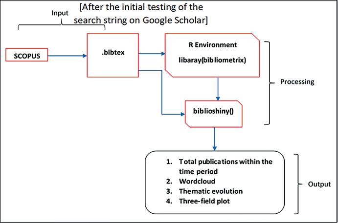
The study is approached from a global point of view. The data for this study were retrieved from the SCOPUS database. The SCOPUS database was used based on its reputation and wide acceptance. Hence, any paper published on the topic in any journal not indexed in SCOPUS would not have been retrieved. The data was downloaded in a .bibtex format, and it contains the title, authors, institutions, abstract, keywords, keywords plus and references, among other things (Fig. 1.1).
1.2.2 Data Retrieval
The dataset in .bibtex format as retrieved for this study from SCOPUS is based on the syntax “grasslands and remote sensing and mountains and biomass” or “grasses and biomass and mountain and remote sensing” or “highlands and grass and
S. Mathapelo et al.
Fig. 1.1 Flowchart showing the methodology and outputs
biomass and earth observation”. The choice of the search syntax is borne out of the focus of the study and careful identifcation of the mix of words on google scholar. The syntax used for the review was tested within Google Scholar for appraisal and stability. After careful sorting and to the satisfaction of the authors, we applied the same search protocol ([grasslands and remote sensing and mountains and biomass] or [grasses and biomass and mountain and remote sensing] or [highlands and grass and biomass and earth observation]) within the SCOPUS database.
This was essential to ensure that studies on the subject were not left out due to the choice of words. Hence, these strings of words form the focus of this study (Fig. 1.1). Therefore, any publication that is not solely on the use of remote sensing techniques for the estimation of grasslands in montane environments will not be retrieved by the search engine. Out of a total of four thousand three hundred and eighty-six (4386) papers published under the syntax “grasslands and remote sensing”, only twenty-four (24) papers have been published so far using the “grasslands and remote sensing and mountains and biomass” or “grasses and biomass and mountain and remote sensing” or “highlands and grass and biomass and earth observation” syntax and indexed in SCOPUS (Fig. 1.1).
1.2.3 Data Analysis
The bibliometrix package in R (Aria & Cuccurullo, 2017) was used to analyse the data (Fig. 1.1) as retrieved from the SCOPUS database. The .bibtex format was converted into a bibliometrix fle using the convert2df () function. The convert2df function converts the .bibtex format into a dataframe with variables such as but not limited to authors, countries, affliations, references, keywords, co-authors and citations. After the conversion, the data was used to initiate the biblioshiny environment using the biblioshiny () function. The biblioshiny environment is a shiny app that provides a web interface for bibliometrix. From the biblioshiny app, document information, authors publication list, wordcloud, three-feld plot and thematic evolution of keywords were generated (Fig. 1.1).
1.3 AGB and RS in Montane Grasslands
There has been considerable progress in the use of optical sensors in the estimation AGB of grasslands (Table 1.1). Optical remote sensing makes use of visible, nearinfrared and short-wave infrared sensors to form images of the earth’s surface by detecting the solar radiation refected from targets on the ground. In simple terms, it makes use of natural radiation from the sun and provides a two-dimensional view of grasslands and other earth surface topographies. Most optical images such as Landsat and Sentinel-2 are freely accessible and affordable and have allowed a large number of studies to freely use the products from these optical sensors. AGB estimation in lowland grasslands has proved successful using either active or passive optical sensors (Niu & Ni, 2003; Ali et al., 2017; Guerini Filho et al., 2020).
Multispectral data such as the Landsat MSS, Landsat TM and Advanced Very High-Resolution Radiometer (AVHRR) has been successfully used in many different areas across the world for estimating grassland biomass (Niu & Ni, 2003; Nguyen et al., 2020); while some others have enhanced grassland biomass estimation with machine learning algorithms (Adepoju & Adelabu, 2020; Silveira et al., 2019), their use in montane grassland studies is largely constrained and remains limited (Table 1.1). These constraints are due to the regular cloud conditions that often restrain the acquisition of high-quality remotely sensed data by optical sensors (Mohd Zaki & Abd Latif, 2017; Xu et al., 2020). Furthermore, vegetation indices (VI) computed from these optical sensors reach a saturation level on high-density biomass estimation (Mutanga & Skidmore, 2004). In their study, on narrow-band vegetation indices, Mutanga and Skidmore (2004) posited that limited channels on multispectral images restrict the estimation of vegetal indices such as the Normalized Difference Vegetation Index (NDVI) because they asymptotically approach a saturation level after a certain biomass density due to growing seasons, a view upheld by several authors (see Mutanga & Skidmore, 2004).
S. Mathapelo et al.
Table 1.1 Biomass estimation: sensors, fndings and references from 2009 to 2020
Sensor(s) Elevation Findings
Optical sensors
Landsat (5, 7, 8)
Montane Landsat archive is a great resource for reconstructing grassland areas, and Landsat improves the estimation of biomass
References
Kuang et al. (2020), Morley et al. (2019), Primi et al. (2016), Barrachina et al. (2015), Borrelli et al. (2015), Elias et al. (2015) and Chen et al. (2014)
MODIS
Montane
The capability of MODIS with or without climatic variables and VI provides a good estimate of biomass across montane environments
RapidEye Montane RapidEye is identifed as a suitable product for biomass estimation and an improvement against some other optical sensors
GeoEye
Sentinel-1
Systéme Pour lObservation de la Terre (SPOT)
Airborne Unarmed aerial vehicle (UAVs) Multi-rotor UAV equipped with Micro-MCA12
Snap Airborne Visible and InfraRed Imaging Spectrometer (AVIRIS)
Montane Applicability of GeoEye in biomass estimation was satisfactory
Montane As with other optical sensors, Sentinel-1 also provides a good estimate for biomass
Montane It was established that the (SPOT) NDVI-biomass relationship can be quantifed effectively and is a good indicator of biomass
Montane
The study analyses the spatiotemporal changes in AGB using UAVs in Tianshan Mountain. The author posited that poor correlations exist between aboveground biomass and VIs, but these correlations improved remarkably after considering the terrain factors Furthermore, using the airborne AVIRIS, Ernst et al. (2003) discriminated against different grass species on the White-Inyo Range, Eastern California. This was later used to understand the relationship between vegetation and climate and geology
Zhang et al. (2018); Kuang et al. (2020), De Leeuw et al. (2019), Yang et al. (2016), Choler (2015), Maselli et al. (2013) and Yan et al. (2021)
Magiera et al. (2017)
Morley et al. (2019)
Morley et al. (2019)
Morley et al (2019) and Klinge et al (2018)
Ernst et al. (2003)
S. Mathapelo et al.
Despite the aforementioned limitations in the use of optical sensors, success has been recorded in the use of GeoEye, RapidEye, Sentinel, SPOT, Landsat and most especially Moderate Resolution Imaging Spectroradiometer (MODIS) (Table 1.1). The level of success recorded has been attributed to but not limited to the use of narrow-band vegetation indices computed from hyperspectral data and high spectral resolutions to estimate biomass (Zhang et al., 2020), especially with some results showing that modifed vegetation indices calculated from the red-edge and nearinfrared shoulder domains can successfully estimate biomass (Table 1.1) as compared to the standard red or infrared-based indices. Cho and Skidmore (2009) in their study conducted within the Majella National Park, Italy, a Mediterranean montane area, between 2004 and 2005 extracted vegetation indices (VIs) (narrow-band NDVI, modifed soil-adjusted vegetation index, NSAVI, and normalized difference water index, NDWI) and also red-edge positions (REP) from HyMap image, an airborne hyperspectral imaging sensor. They concluded in their study that VIs are a weak predictor of grass/herb biomass within their study area. However, they concluded that narrow bands in the red-edge positions are more consistent predictors of biomass estimations in montane grasslands. The limitations regarding hyperspectral data sources include but are not limited to cost, availability, processing and high dimensionality.
Generally, whether it is hyperspectral or multispectral, Lu (2006) and Wu et al. (2016) affrmed that the use of moderate to coarse spatial resolution sensors such as Landsat, MODIS and AVHRR for AGB estimation especially in montane grassland results in poor forecast accuracy. This is because of the occurrence of mixed pixels composed with a mismatch between the size of sections and the pixel since the area consists of different landscapes. However, despite these limitations, passive optical sensors are still the frst point of call for most AGB estimations because of availability, free-to-low-cost, coverage and spectral resolution.
1.4 BGB and RS in Montane Grasslands
Below-ground biomass (BGB) is the biomass totality of live roots except for those roots less than 2 mm in diameter. Live roots less than 2 mm in diameter are largely excluded because of the yet-to-be verifed difference between these roots and soil organic matter. Globally, BGB accounts for about 20% of the total biomass. Therefore, the direct estimation of below-ground biomass is very important especially in estimating the total carbon pool and understanding carbon loss and storage for specifc environments. Conventionally, the following methods are used in the estimation and monitoring of BGB. These are the excavation of roots, monolith for deep roots, soil core or pit for non-tree vegetation, root-to-shoot ratio and allometric equations (Fan et al., 2008; Peng et al., 2020). BGB estimations for most grassland studies have employed the above-listed methods or a combination of feld-based studies (Fan et al., 2008; Peng et al., 2020).
Compared to AGB, BGB of grassland communities is still growing in the literature. The use of remote sensing techniques in the estimation of BGB is still growing even for lowland studies. Chapungu et al. (2020) estimated BGB of savanna grasslands using an indirect relationship between AGB and BGB and then comparing that with NDVI. In their study, they stated the limitations of multispectral data especially those obtained from Landsat images. They concluded that for grassland biomass estimation, multispectral sensors of Sentinel-2 and Worldview-3 hold great promise using the red-edge region. For montane environments, BGB estimations for grasslands are few and far in between. There is a need for studies on BGB estimations for montane grasslands using remote sensing techniques to fully understand these unique ecosystems and their dynamics.
1.5 Grasslands Biomass Estimation in Montane Environments: Global Knowledge
Globally, the state of knowledge with regard to biomass estimations in montane environments is just growing. The frst paper emerged on the global scene in 2003 (Table 1.2). The highest number of papers, fve (5) in total, was published in the year 2015 and then three published in the year 2018; every other year had less than three publications (Table 1.2). The growth of papers in biomass estimation of grasslands in montane environments has not been very great, and the reasons could be but not limited to the terrain, available sensors and the importance attached to this ecosystem. From these studies, the platform for data extraction has been mainly from space (satellites), while only two studies have made use of airborne instruments (Sun et al., 2018).
On the global scene, some authors have contributed greatly to the subject matter. These authors such as Magiera, A., Feilhauer, H., Waldhardt, R., Wiesmair, M., Otte, A, Barrachina, M and Zhang, Y (Fig. 1.3), have published at least two papers on the subject matter. Across the available studies, most of the keywords outside grasslands, remote sensing and biomass have been on but not limited to some parts of China and Italy.
Attempting a spatio-temporal evolution of these keywords reveals how over time (2003–2020), there has been growth in the direction of studies on grasslands, biomass and remote sensing in montane environments (Fig. 1.2). Studies involving carrying capacity, ecosystems and spatial distribution entered the narrative of studies on grasslands within montane environments using remote sensing in 2016. Since 2016, these words have stayed to date. However, there has been little concern about below-ground biomass. The focus has been on aboveground biomass, primary production of grasslands within these environments. The most prominent sensor has been the MODIS, while the only machine learning tool observed between the period is the random forest (Fig. 1.3). 1 Montane Grasslands: Biomass Estimations Using
Table 1.2 Progression of publications from 2003 to 2020
Year No and title(s)
2003 1. Reindeer Pasture Biomass Assessment Using Satellite Remote Sensing
2. Relationships among vegetation, climatic zonation, soil, and bedrock in the central White-Inyo Range, eastern California: A ground-based and remote-sensing study
2009 1. Infuences of changing land use and CO2 concentration on ecosystem and landscape level carbon and water balances in mountainous terrain of the Stubai Valley, Austria
2010 1. Spatial Analysis of Fire Potential in Iran Different Region by Using RS and GIS
2. Development of new vegetation indexes, shadow index (si) and water stress trend (wst)
2011 1. The correlation analysis between herbage yield and ecoclimatic factors and carbon storage accounting of desert grassland in Xinjiang, China
2013 1. Simulation of grassland productivity by the combination of ground and satellite data
2014 1. The application of grassland aboveground biomass estimating model in Karst mountainous area
2015 1. Estimating above-ground biomass on mountain meadows and pastures through remote sensing
2. The implications of fre management in the andean paramo: A preliminary assessment using satellite remote sensing
3. Land conversion dynamics in the borana rangelands of southern Ethiopia: An integrated assessment using remote sensing techniques and feld survey data
4. Growth response of temperate mountain grasslands to inter-annual variations in snow cover duration
5. 2015 8th International Workshop on the Analysis of Multitemporal Remote Sensing Images, Multi-Temp 2015
2016 1. Monitoring of grassland herbage accumulation by remote sensing using MODIS daily surface refectance data in the Qingnan Region
2. From Landsat to leafhoppers: A multidisciplinary approach for sustainable stocking assessment and ecological monitoring in mountain grasslands
2017 1. Modelling biomass of mountainous grasslands by including a species composition map
2. Natural mowing grassland resource distribution and biomass estimation based on remote sensing in Hulunber
2018 1. Mapping Plant Functional Groups in Subalpine Grassland of the Greater Caucasus
2. Climate effects on vegetation vitality at the treeline of boreal forests of Mongolia
3. Estimating aboveground biomass of natural grassland based on multispectral images of Unmanned Aerial Vehicles.
2019 1. Application of the MODIS MOD 17 Net Primary Production product in grassland carrying capacity assessment
2. Quantifying structural diversity to better estimate change at mountain forest margins
2020 1. A remote sensing monitoring method for alpine grasslands desertifcation in the eastern Qinghai-Tibetan Plateau
2. Spatial distribution pattern of NPP of Xinjiang grassland and its response to climatic changes
1.6 Issues and Challenges in Africa
The issues and challenges surrounding African grasslands can be conceptually captured using the DPSIR (Drivers, Pressures, State, Impact and Response) Framework (Agyemang et al., 2007). The grasslands of Africa are savannas asides from the velds of Southern Africa. The savanna in Africa is the most extensive in the world
S. Mathapelo et al.