RGS_The_Journal_2025

FROM THE HEADMASTER

For those of a certain vintage, brought up on a diet of novels set in Victorian public schools, scholarship is a rather quaint, old-fashioned concept. Scholarship is associated with row upon row of dusty, leather-bound editions of obscure textbooks, immaculately laid out in a rather grandiose, oak-panelled library. Scholarship is synonymous with ageing, rather austere schoolmasters sporting tweed blazers, elbow patches and half-moon spectacles. Scholarship is elitist and rooted in weighty tomes.

The Latin Inscription in School Room AUT DISCE AUT DISCEDE (Either learn or leave) would simply seem to reinforce this impression of scholarship.

And yet this impression could not be further from the truth at the RGS in the 21st century. Our recent inspection highlighted scholarship as one of the School’s two Significant Strengths: “pupils develop a breadth of knowledge and enthusiasm for scholarship… This strong academic culture leads to pupils who readily engage in critical thinking and deep learning and display intellectual curiosity.” If you were looking for evidence, then this edition of The Journal could not be a better illustration of how vibrant students’ learning and research is. Far from an outdated concept, scholarship at the RGS is dynamic and cutting edge, relevant and exciting, enriching and innovative, irrespective of where a student’s passion may lie.

I would like to take this opportunity to thank Mrs Tarasewicz, our Head of Scholarship, for her hard work and inspiration in compiling this impressive publication, to Mrs Webb for designing and producing this, and - most of all - to all those students who have contributed articles which are the result of so much passion, research and reflection. Scholarship - an outdated concept? Nothing could be further from the truth!

Dr JM Cox Headmaster

'SCHOLARSHIP FOR ALL'

JOEL SELLERS - ORIS

THOMAS DOWSON - STEM

RUVIN MEDA - ARTS

FROM THE HEAD OF SCHOLARSHIP

Welcome to this year’s edition of The Journal.

One of the joys of working in education is that no two days are the same. Nonetheless, every year I am delighted anew by the variety and sheer calibre of the ILA (Independent Learning Assignment) and ORIS (Original Research in Science) projects that our Sixth Form students produce. So high was the quality of submissions this year that we had to introduce an additional stage in the shortlisting process when trying to select students to take part in the ILA/ ORIS Presentation Evening, when the top students have the chance to compete for the coveted ILA and ORIS awards. It is this carefully selected shortlist of students that have been included in this publication and it gives me the greatest pleasure to share such a diverse, fascinating and frankly outstanding collection of essays with you.

As you will find in exploring the pages of this magazine, the eventual winners of the ILA and ORIS awards were Ruvin Meda in the ILA Arts and Humanities category, Thomas Dowson in the ILA STEM category and Joel Sellers in the ORIS category, which was recognised separately for the first time this year. Special mention should be made of Ruvin because his full ILA cannot be included in the way that the others have been. This is because Ruvin’s ILA was, in fact, a film music score! Those of us at the ILA/ORIS Presentation Evening had the delight of listening to this, whilst watching the film that it accompanied, which was truly magical. Not only did Ruvin win our internal ILA award, but his composition was also recognised externally, securing second place in the Guildhall School of Music & Drama Release 2024 competition.

The calibre of work that the students produce for their ILA and ORIS projects indicates the strength and value of this programme. It therefore gives me great pleasure to report that this year, for the first time, we have also launched a Junior ILA (ILA JNR), open to all students in the Third and Fourth Forms. These younger students will each be supported by a Sixth Form mentor as they undertake a piece of independent research - perhaps their first piece of truly independent research - on a topic of their own choosing. We have been absolutely delighted by student uptake and look forward to sharing their work with an audience of friends and families at the Junior ILA Celebration Event at the start of the Trinity Term.

As last year, my particular thanks go the Georgina Webb, our Partnerships and Publications Assistant, for her flare and precision in producing such an eye-catching edition of The Journal. My thanks also go to Peter Dunscombe and Wai-Shun Lau for their continued support with running the ILA and ORIS programmes.

I very much hope that you enjoy the selection of projects that we have drawn together for you. Happy reading!

Mrs HE Tarasewicz Head of Scholarship

With thanks to: Mr Dunscombe, Mr Lau, Mrs Farthing and all of the ILA supervisors for their support with the ILA and ORIS programmes.

JOEL SELLERS WINNER OF ORIS

STEM

SCIENCE . TECHNOLOGY

ENGINEERING . MATHEMATICS

THOMAS DOWSON WINNER OF STEM

AN EVALUATION OF CAR T-CELL THERAPY AS A PROMISING NEW ROUTE FOR IMMUNOLOGICAL CANCER TREATMENTS

STEM

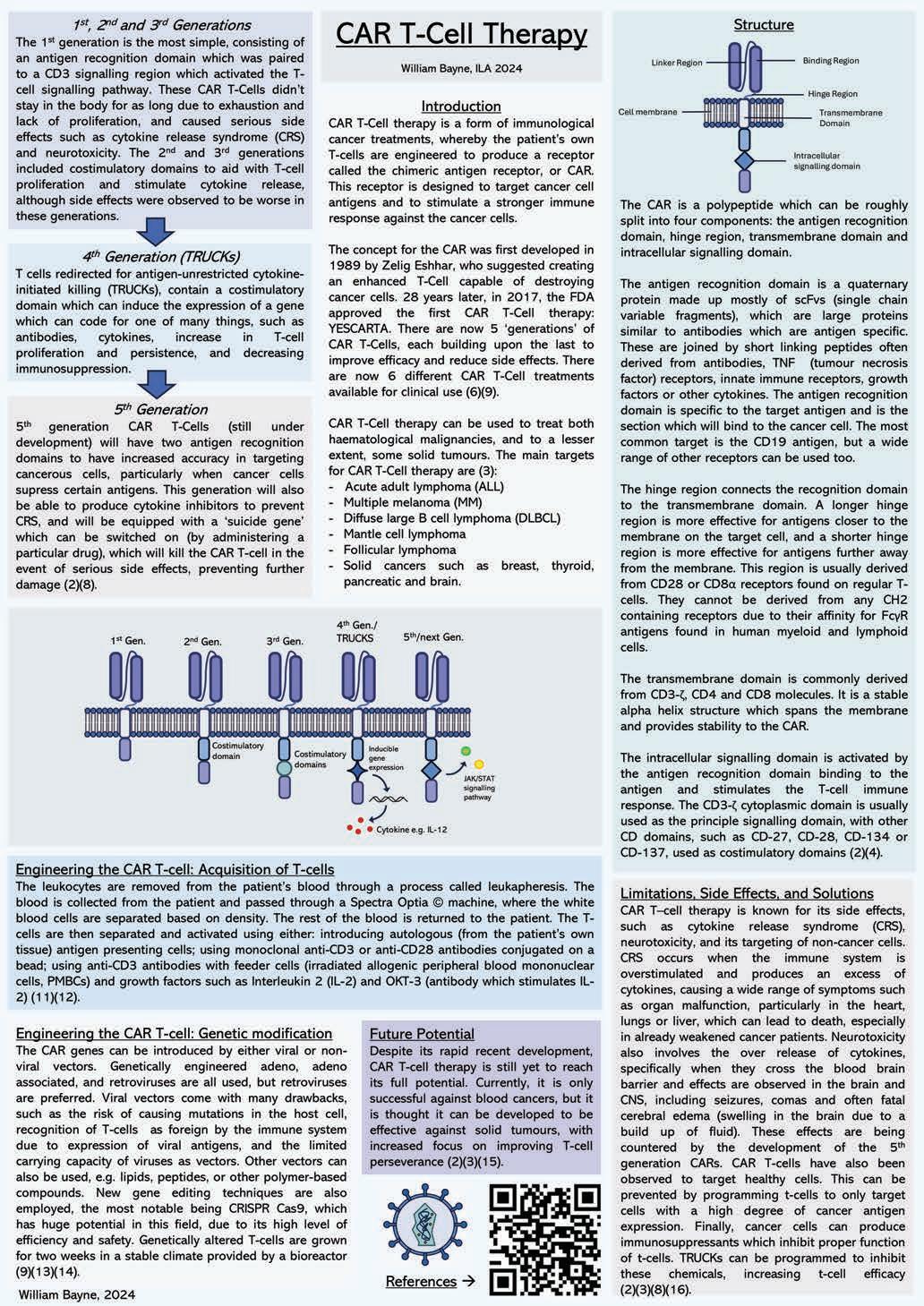
WILLIAM BAYNE

This Independent Learning Assignment (ILA) was short-listed for the ILA/ ORIS Presentation Evening.

INTRODUCTION

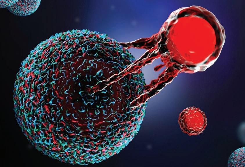
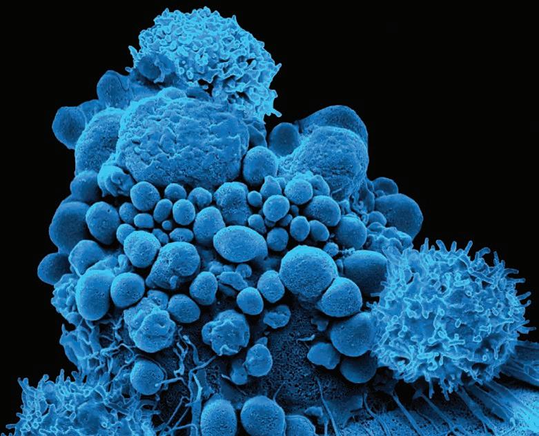
Immunotherapy is a relatively cutting-edge form of cancer treatment, having only been approved for use in the last 7 years. Unlike other common treatments for cancer which generally employ the tactic of directly killing or removing large numbers of cells from the tumour, immunotherapy works in a more subtle way. As the name suggests, it involves aiding the immune system in fighting and killing the

cancer cells. This can be done in many ways, from utilising immune checkpoint inhibitors, to creating a vaccine which will specifically target cancerous cells, or creating genetically enhanced white blood cells specifically designed to stimulate an immune response against cancer cells - CAR (Chimeric Antigen Receptor) T-cell therapy.1

STRUCTURE OF THE CHIMERIC ANTIGEN RECEPTOR AND ITS EVOLUTION

The first research into this type of treatment began in the 1980s, with scientists such as Zelig Eshhar suggesting the first plans for creating an enhanced T-cell capable of destroying cancer cells in 1989. However, it was not until 2017 that the FDA approved the first CAR T-cell treatment for clinical use, YESCARTA.9 Since 1989, the chimeric antigen receptor has come a long way, with five recognised 'generations' of CARs, each more effective and with fewer side effects than the last.

CAR T-cell treatment is used to treat a wide range of cancer types, both haematological malignancies and some solid tumours,3 although different types of CAR T-cells are used for different types of cancer, due to the absence or presence of certain antigens on different cancers and the specificity required from the receptor to bind to the antigen.2 There are currently six CAR T-cell treatments available, and are used for the treatment of multiple cancers: Acute adult lymphoma (ALL), Multiple melanoma (MM), Diffuse large B cell lymphoma (DLBCL), mantle cell lymphoma and follicular lymphoma,15 and some solid cancers such as pancreatic, brain, breast and thyroid cancer.23

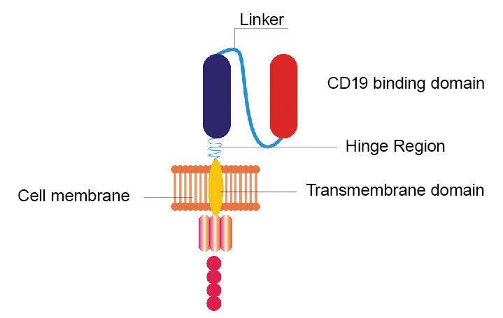
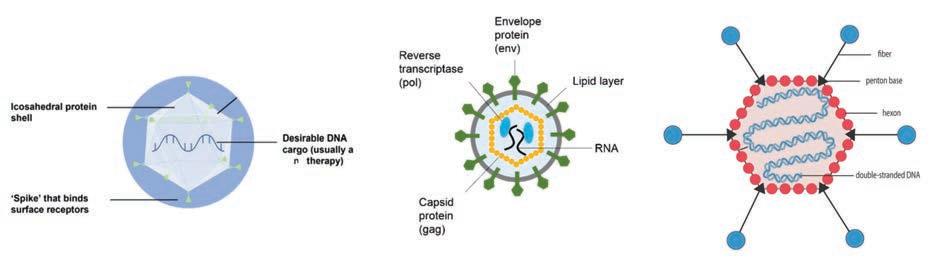
The chimeric antigen receptor (CAR) is a polypeptide made up of multiple components: the antigen recognition domain, the hinge region, the transmembrane domain, and the endodomain.4 The antigen recognition domain is found on the outside and is specific to a particular antigen found on a cancerous cell. It has a quaternary structure made up of single chain variable fragments (scFvs), which are large antigen specific proteins similar to antibodies. These are connected by short linking peptide chains, and are often derived from antibodies, although they can also be obtained from structures such as TNF receptors, innate immune receptors, growth factors or other cytokines.4 It is this section which will recognise and bind to the cancer cell and activate the immune response. The most common target antigen is CD19, but there is a wide range of possible antigens which could be targeted.2

Figure 1: A structure showing the basic structure of the receptor4

The hinge (or spacer) region is found between the antigen recognition domain and the cell surface membrane on the T cell. It can vary in length, but the longer length is preferable for binding regions that are closer to the membrane on the target cell as it lends more flexibility to the antigen recognition domain , however shorter hinge regions are more desirable for antigens with a binding region which is further away from the cell surface membrane. The spacer region is commonly derived from CD28 or CD8α receptors (found on regular T-cells), however they cannot be derived from Immunoglobin G or any other CH2 containing receptors due their affinity for FcγR antigens found on human myeloid and lymphoid cells, which would cause them to bind these cells with many harmful effects.4

The transmembrane domain, as the name suggests, bridges the cell surface membrane of the T-cell and is derived from a wide range of molecules, including, but not limited to, CD3-ζ, CD4 and CD8. It is a stable alpha-helix structure which spans the membrane and stabilises the CAR.4

Finally: the intracellular signalling domain or endodomain. This section, found within the cytoplasm and attached to the transmembrane domain, is responsible for activating the T-cell when the extracellular antigen recognition domain is activated by an antigen. The CD3-ζ cytoplasmic

domain is used for the principal signalling domain, with other CD domains used as co-stimulatory domains, which is required for CAR T-cells to become activated. Commonly used co-stimulatory domains include CD-27, CD-28, CD-134 and CD-137.4

First, Second and Third Generation CAR T-cells

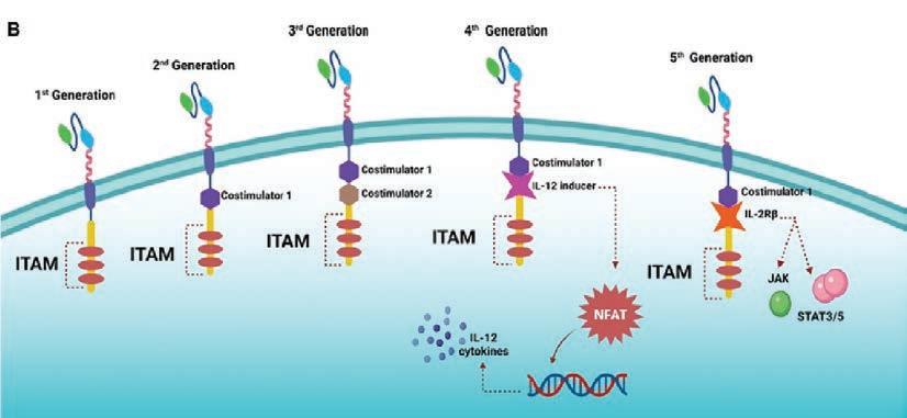
The first generation of CAR T-cells was developed in the 1990s and was the most basic form of CAR T-cells. The CAR was composed of an antigen recognition domain derived from an antibody which would activate the T-cell receptor signalling pathway (CD3-ζ) when coupled with the target antigen and cause an immune response. However, the first generation CARs were less adept at staying in the body for a prolonged period, due to T-cell exhaustion and a lower rate of proliferation, and had limited success against solid tumours and some forms of cancer which lack the target antigen, and were observed to produce some serious side effects such as cytokine release syndrome and neurotoxicity due to a reaction from the immune system against the engineered cells.2/8 In the second and third generations, costimulatory domains were added to aid with T-cell action, by stimulating cytokine release and causing further T-cell proliferation, although more side effects (such as Cytokine Release Syndrome) were observed in the third generation due to a higher production rate of cytokines by the T-cell.2

Figure 2: Proportion of target antigens used in clinical CAR T-cell trails 2

Fourth Generation CAR T-cells, or TRUCKs

Fourth generation CAR T-cells are also called T cells redirected for antigen-unrestricted cytokine-initiated killing, or TRUCKs. TRUCK CARs contain the extracellular antigen recognition domain and the two intracellular signalling domains (one for T-cell activation and one co-stimulatory for cytokine release and T-cell proliferation), as with the second generation. The fourth generation are also engineered with an inducible gene expression which becomes active upon recognition of the antigen. This gene expression system can be engineered to code for many different cytokines or antibodies with a range of functions, such as increasing T-cell proliferation, aiding with T-cell persistence or overcoming immunosuppression. These TRUCKs have much more success in killing tumour cells due to their ability to improve cytotoxicity of the T-cells and increase the number of immune cells at the cancer site, as well as the invaluable tool to decrease immunosuppression caused by the cancerous cells.2

Fifth Generation CAR T-cells

The most advanced CAR T-cell therapy currently under development, the fifth generation of CAR T-cells has many modifications which will allow it to fight cancer with amplified efficiency, strength and safety. One improvement is that the fifth generation will have two antigen recognition domains instead of only one. This means that it is much less likely for the CAR T-cell to falsely recognise other cells as cancer cells if they contain the same antigen. It also means that if the cancer cells become resistant to the T-cell by reducing the number of the target antigens

present on the cell surface, the CAR T-cell will still bind via the other receptor, thereby reducing the effects of resistance to the therapy by the cancer cells. This also means that these CAR T-cells can bind to a larger number of cancer cells as they have a wider target range of antigens, so they can kill cancer cells at a faster rate. The fifth generation also has an improved signalling domain which means the CAR T-cell can act with a more potent ability to recognise and attack cancer cells, due to signalling domains with an increased emphasis on cytokine production and T-cell survival and proliferation2

Fifth generation CAR T-cells are also equipped with tools to help prevent side effects common in earlier generations. They are engineered with the ability to produce cytokine inhibitors which can help control cytokine release syndrome which is a common but sometimes fatal side effect of CAR T-cell therapy.2 They also have the ability to 'commit suicide' in the case of excessive and dangerous side effects. The CAR T-cells can be equipped with one of many methods of suicide such as a suicide gene, which would contain the code for a destructive enzyme such as herpes simplex virus thymidine kinase, or small molecule assisted shutoff (SMASh) where a viral protease and a protease inhibitor are bound to the CAR in a position to cleave the CAR and destroy the cell.8 In all cases for a suicide mechanism, the system will be activated by a particular drug given to the patient in the event of CAR T-cell over expression, making the process much safer.

Figure 3: The evolution of the CAR T-cell from 1st to 5th generation Alnefaie, A. et al. (2022)

ENGINEERING THE CAR T-CELL

Acquisition of T-cells

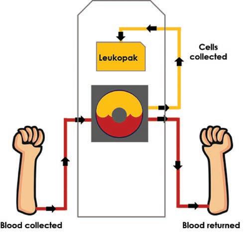
Blood is removed from the patient and the leukocytes (white blood cells) are removed from the blood using a Spectra Optia © machine, which separates the white blood cells based on their density, and the rest of the blood is returned to the patient.9/10 This process is called leukapheresis. The desired T-cells are then separated and activated by one of several methods: introducing autologous (from the patient’s own tissue) antigen presenting cells; using beads containing anti-CD3 and anti-CD28 monoclonal antibodies; or using anti-CD3 antibodies alongside feeder cells (irradiated allogenic peripheral blood mononuclear cells, PMBCs) and growth factors, such as Interleukin 2 and OKT-3 (a monoclonal antibody which stimulates IL-2 and aids with T-cell proliferation).11/12

Introducing the Desired Genes

The CAR genes are inserted into the T-cells either by viral or non-viral vectors. Viral vectors are preferable because of the high rate of genetic transfer of genetic material into the target cells. The CAR gene is inserted into the viral genome and the viral enzymes allow it to integrate the gene into the genome of the T-cells.

Genetically engineered retroviruses, adenoviruses and adeno-associate viruses are used for this, with retroviruses the preferred type. However, viral vectors have their drawbacks: the insertion of the gene into the host cell genome can lead to mutations which have the potential to cause the formation of a tumour; the virus can also cause the T-cell to be recognised as a foreign cell by the patient’s immune system leading to an undesired immune response; due to the small size of viruses, only smaller, less complex genes can be used, which restricts the potential for CAR T-cell therapy using viral vectors; the viruses can also find it difficult to produce high concentrations of genetically engineered cells.9

Non-viral vectors are also used, due to their unlimited carrying capacity and non-infectiousness. Vectors include lipid, peptide, and polymer-based compounds, alongside nude DNA and minicircle DNA. These generally work by chemically aligning themselves with a part of the DNA molecule though hydrophobic or hydrophilic interactions, at which point the DNA section is inserted into the genome.14

This section of CAR T-cell therapy has also improved with the development of new genetic engineering methods such as CRISPR Cas9, which has huge

Figure 4: A diagram outlining the procedure for leukapheresis 11

potential for the reduction of current limitations of CAR T-cell therapy due to its accessibility and simplicity, not to mention improved safety compared to viral vectors.13 It is also much more effective at allowing for an introduction of higher numbers of genetically engineered T-cells (i.e a higher concentration of T-cells which have been genetically engineered) to the patient, as hence a stronger and more efficient treatment. Once the CAR T-cells are created, they are allowed to grow for two weeks in a Bioreactor system so they can multiply to a very large number. They are delicate cells however so require a stable microclimate to grow in, which can be provided by certain types of Bioreactors.9

POTENTIAL AND LIMITATIONS

Although CAR T-cell therapy has come a very long way since it was first conceived in 1989, its still has not reached its full potential. Currently, T-cell therapies are only successful against certain haematological cancers such as ALL (adult acute lymphoblastic leukaemia), MM (multiple melanoma), DLBCL (diffuse large B cell lymphoma), mantle cell lymphoma and follicular lymphoma, and some solid tumours such as pancreatic, breast, thyroid and brain cancers.15/23 Despite this, it is thought that CAR T-cell therapy can be developed far enough to be effective against more types of solid tumours3, especially with the rapid advancements constantly being made to increase the stamina of T-cells in fighting the cancer cells ). Often in patients undergoing CAR T-cell therapy, T-cells can become exhausted, but this issue is reduced with each generation of CARs.2 CAR T-cell therapy can also suffer from resistance to the treatment by cancer cells, where the target antigen becomes less expressed, reducing the effect of the CAR T-cell. This can be combated by introducing a second antigen receptor region to the CAR so that the T-cell has

“ The past thirty-five years have seen a dramatic development in the field of immunotherapy, with five separate generations of CAR T-cells developed, and six treatments currently approved by the FDA.

a second region to bind to if the cancer cell downplays the expression of one antigen, increasing its efficacy. CAR T-cell therapy is also known for its side effects, such as cytokine release syndrome, neurotoxicity and targeting of non-cancer cells, to name a few. Cytokine release syndrome (CRS) occurs due to overstimulation of the immune system to produce too many cytokines (cell signalling molecules), resulting in a wide range of symptoms, from inflammation to organ malfunction, particularly in the heart, lungs and liver, which in many cases (especially in already weakened cancer patients), can lead to death. Neurotoxicity also occurs due to an increase in cytokine production, specifically when the blood-brain barrier is crossed and adverse effects are observed in the brain and CNS, including seizures, comas and often fatal cerebral edema (swelling in the brain due to a build-up of fluid).16 Both these side effects are already starting to be dealt with in the 5th generation CAR T-cells which can both inhibit cytokines in the event of CRS and can be easily 'switched off' if the side effects are very serious.8 CAR T-cells have also been seen to attack some healthy body cells which can often display the same antigens as cancer cells, which leads to many harmful effects. This effect can be reduced by programming the T-cells to recognise cells with higher degree of antigen expression as would be in the tumour cell but not in regular body cells.3 Finally, the problem of immunosuppressants released by the cancer cells, preventing the proper function of the T-cells. This can be combated by producing CAR T-cell which are resistant to such chemicals, as was developed to a certain degree in the fourth generation.2

CONCLUSION

The past thirty-five years have seen a dramatic development in the field of immunotherapy, with five separate generations of CAR T-cells developed, and six treatments currently approved by the FDA. Each generation of CARs brings a new weapon to the fight against cancer, whether that be the ability to increase T-cell numbers more rapidly, inhibit immunosuppressants, or increase the safety of the patient during the treatment by managing the side effects. The process for creating these CAR T-cells is also evolving constantly, with the development of CRISPR technology helping this process become much faster, safer and efficient, and with advancements in the biomedical industry occurring at such a high rate, I would expect to see a dramatic increase in the success of this type of therapy in the near future.

APPENDICES:

Appendix A: Abbreviations and definitions (in order of appearance)

• CAR: chimeric antigen receptor.

• Chimeric: coded for by more than one different gene.

• CD (followed by a number): cluster of differentiation, a term given to a cell surface antigen or group of antigens, and the receptors which would bind to them.

• CH: Constant heavy chain

Appendix B: Other cancer treatments

• Chemotherapy uses drugs which will usually inhibit particular stages in the cell cycle, thereby preventing cancer cells (cells undergoing uncontrolled mitosis) from undergoing mitosis, preventing growth of the malignancy or tumour. However, despite the fact that these drugs can be targeted to the cancer cells, this can still also damage other cells in the body, causing severe side effects. Radiotherapy uses radio waves to kill cancer cells. However, this is a destructive process which can easily damage other body cells. Surgery is also commonly used to treat cancer but is often difficult, sometimes unsuccessful, and also not possible for many types of cancer, e.g haematological malignancies.

Appendix C: Immunoglobin G, CD2 and delocalised attack

• Immunoglobin G (IgG) contains CH2 receptors which will bind to FcγR antigens present on myeloid and lymphoid cells. Myeloid cells include macrophages, megakaryocytes granulocytes and erythrocytes, while lymphoid cells include T-cells, B-cells and natural killer cells6. These cells will be targeted by the CAR T-cells as well as the cancerous cells, leading to a decreased frequency of attack on the cancer cells by the CAR T-cells, and therefore decrease effectiveness of the treatment.

There have been in vivo studies to show that by removing the CH2 from the IgG the delocalisation of attack of CARs can be reduced7, but the most effective way of reducing this is to just use other sources for the hinge region.

Appendix D: The use of viral vectors in the genetic engineering of T-cells

• Three main types of viral vectors are used for gene transfer to T-cells: retroviruses, adenoviruses and adeno-associated viruses. They all have a similar structure but are differentiated by the form of genetic material which is contained by the virus. Retroviruses contain a portion of single stranded RNA19, which is made into DNA inside the host cell using the virus’ enzymes, ready to be integrated into the host genome. Adenoviruses do not store genetic information as RNA but rather as double stranded DNA20, thereby eliminating the need for a conversion from RNA to DNA in the host genome. Adeno-associated viruses (AAVs) are subtly different in that they contain single stranded DNA instead of double stranded DNA21

Figure D: Left to right: structure of a retrovirus19, an adenovirus20 and an adeno-associated virus21 (simplified)

In all cases, the original viral genetic material is removed from the virus and replaced with the desired genetic material. This is to prevent viral replication inside the T-cells, which would likely result in cell death.

Appendix E: Side effects: cytokine release syndrome (CRS) and neurotoxicity in more detail

• CRS is a common side effect of CAR T-cell therapy and is characterised by a high release of cytokines into the blood. This can cause mild to serious side effects, from flu or fever- like symptoms to severe hypoxia and capillary leakage, with many more symptoms also reported22. Although the exact mechanism for CRS is poorly understood, certain aspects of the syndrome can be derived from the symptoms and the levels of certain cytokines found in CRS patients. For example, IL-6 (among others) is likely to result from activation of the endothelial cells and results in an immune response targeting these cells. This can lead to capillaries leaking and low blood pressure (hypotension)22. The cause of some other symptoms of CRS could also be derived in a similar way.

In most cases of neurotoxicity following CAR T-cell therapy, it is a result of CRS and is characterised by decreased integrity of the blood brain barrier due to CRS. Like CRS, the symptoms range from mild to serious, with some patients only suffering from slight confusion or aphasia (difficulties speaking or understanding others speaking), to seizures and cerebral edema (swelling due to fluid build-up)22

Appendix F: Costs associated with CAR T-cell therapy compared to other treatments

• An important factor to consider is the high cost to success ratio compared to other forms of cancer treatment. CAR T- cell therapy can cost as much as $500,000 for some patients17, compared to a 6-month course of chemotherapy which is estimated to cost around $27,000 (18), and with little guarantee of a side effect free treatment, with the highest CRS rate being 95% in for one particular treatment17. This begs the question as to whether this form of treatment is really worth the cost.

BIBLIOGRAPHY:

1. National Cancer Institute (no date) Immunotherapy for Cancer - NCI. Available at: https://www.cancer.gov/about-cancer/ treatment/types/immunotherapy (Accessed: June 4, 2024).

2. Wang, C. et al. (2023) CAR-T cell therapy for hematological malignancies: History, status and promise, Heliyon, 9 (11).

3. Alnefaie, A. et al. (2022) Chimeric Antigen Receptor T-Cells: An Overview of Concepts, Applications, Limitations, and Proposed Solutions, Frontiers in Bioengineering and Biotechnology, 10.

4. Ahmad, U. et al. (2022) Chimeric antigen receptor T cell structure, its manufacturing, and related toxicities; A comprehensive review, Advances in Cancer Biology - Metastasis, 4.

5. Novartis (2017) Novartis receives first ever FDA approval for a CAR-T cell therapy, Kymriah (TM) (CTL019), for children and young adults with B-cell ALL that is refractory or has relapsed at least twice | Novartis. Available at: https://www.novartis.com/news/ media-releases/novartis-receives-first-ever-fda-approval-car-t-celltherapy-kymriahtm-ctl019-children-and-young-adults-b-cell-allrefractory-or-has-relapsed-least-twice (Accessed: June 6, 2024).

6. Kondo, M. (2010) Lymphoid and myeloid lineage commitment in multipotent hematopoietic progenitors, Immunological reviews, 238 (1), p.37.

7. Pastrana, B., Nieves, S., Li, W., Liu, X. and Dimitrov, D.S. (2020). Developability assessment of an isolated CH2 immunoglobulin domain, Analytical chemistry, 933, pp.1342-1351.

8. Andrea, A.E., Chiron, A., Bessoles, S. and Hacein-Bey-Abina, S. (2020). Engineering next-generation CAR-T cells for better toxicity management, International journal of molecular sciences, 21(22), p.8620.

9. Zhang, C., Liu, J., Zhong, J.F. and Zhang, X., (2017). Engineering car-t cells Biomarker research, 5, pp.1-6.

10. Thompson, J. (2020). What is leukapheresis? Caltag Medsystems. Available at: https://www.caltagmedsystems.co.uk/information/ what-is-leukapheresis/ (Accessed: 12 June 2024).

11. Jin, C., Yu, D., Hillerdal, V., Wallgren, A., Karlsson-Parra, A. and Essand, M., (2014). Allogeneic lymphocyte-licensed DCs expand T cells with improved antitumor activity and resistance to oxidative stress and immunosuppressive factors. Molecular Therapy-Methods & Clinical Development, 1.

12. Schwab, R.I.S.Ë., Crow, M.K., Russo, C.A.R.L.O. and Weksler, M.E., (1985). Requirements for T cell activation by OKT3 monoclonal antibody: role of modulation of T3 molecules and interleukin 1. Journal of immunology (Baltimore, Md.: 1950), 135(3), pp.1714-1718.

13. Dimitri, A., Herbst, F. and Fraietta, J.A., (2022). Engineering the next-generation of CAR T-cells with CRISPR-Cas9 gene editing Molecular cancer, 21(1), p.78.

14. Ramamoorth, M. and Narvekar, A., (2015). Non viral vectors in gene therapy-an overview Journal of clinical and diagnostic research: JCDR, 9(1), p.GE01.

15. Cancer Research UK (2024) Blood cancers | Cancer Research UK. Available at: https://www.cancerresearchuk.org/ about-cancer/blood-cancers (Accessed: June 12, 2024).

16. Gust, J., Ponce, R., Liles, W.C., Garden, G.A. and Turtle, C.J., 2020. Cytokines in CAR T cell–associated neurotoxicity Frontiers in Immunology, 11, p.577027.

17. Choi, G., Shin, G. and Bae, S., 2022. Price and prejudice? The value of chimeric antigen receptor (CAR) T-cell therapy. International Journal of Environmental Research and Public Health, 19(19), p.12366.

18. Geng, C. (2023) Cost of Chemotherapy: What to expect and financial help, Medical News Today. Available at: https://www.medicalnewstoday.com/articles/ chemotherapy-cost (Accessed 19 June 2024)

19. Ulbrich, M. et al. (2014). The Viral Vector. Available at https://2014.igem.org/Team:Freiburg/Project/ The_viral_vector (Accessed 19 June 2024)

20. Applied Biological Materials (No date). The Adenovirus System. Available at: https://info.abmgood.com/adenovirussystem-introduction (Accessed 19 June 2024)

21. Blair, P. (No date). Snapshot: what are adeno associated viruses (AAV)? Available at https://www. ataxia.org/scasourceposts/snapshot-what-are-adenoassociated-viruses-aav/ (Accessed 19 June 2024)

22. Freyer, C.W. and Porter, D.L., 2020. Cytokine release syndrome and neurotoxicity following CAR T-cell therapy for hematologic malignancies Journal of Allergy and Clinical Immunology, 146(5), pp.940-948.

23. Jogalekar, M.P., Rajendran, R.L., Khan, F., Dmello, C., Gangadaran, P. and Ahn, B.C., 2022. CAR T-Cell-Based gene therapy for cancers: new perspectives, challenges, and clinical developments Frontiers in immunology, 13

STEM THOMAS DOWSON WILL KNOT THEORY PAVE OUR FUTURE?

This Independent Learning Assignment (ILA) won the ILA prize in the STEM category

INTRODUCTION

A knot is a simple yet complex object, which can be found almost anywhere in the world. If you have ever been climbing I’m sure you can appreciate the power a knot has. Can a knot be more than just a rope used as a safety measure for people who can’t climb?

If we look at a knot, surely there must be some way of describing it. Looking at the dictionary definition it states:

"A join made by tying together the ends of a piece or pieces of string, rope, cloth, etc".

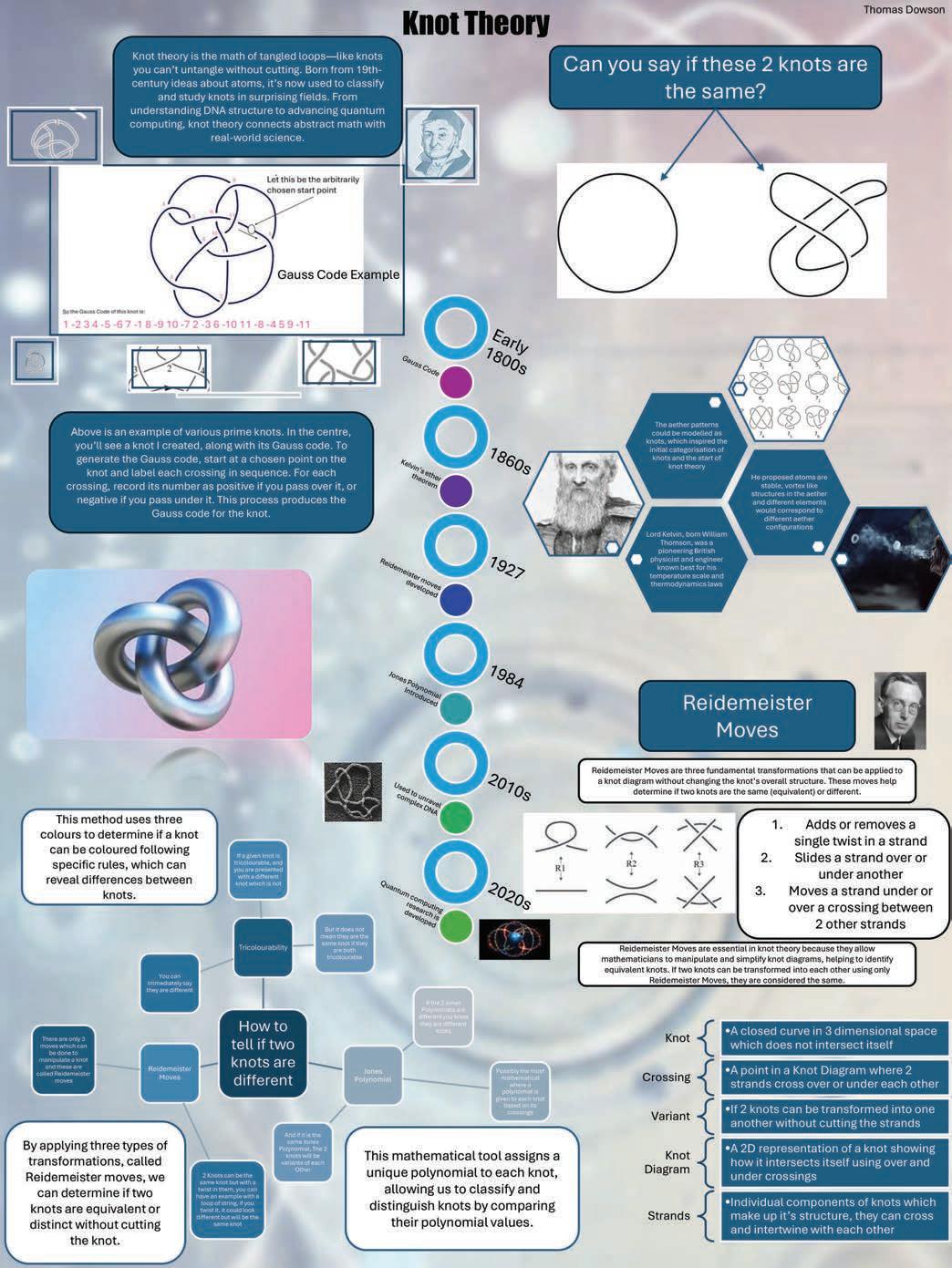
In comes Knot theory, a constantly developing branch of mathematics and physics. Where advances are being constantly made in the quantum branch with new knot variants and invariants being discovered, and quantum fields and gravity being developed consequently. Although quantum might seem unfamiliar to many, knot theory finds applications across various fields of science. Both computer science and mathematics feature specialized branches dedicated to the study of knots.

Gilbert Boro - Flat Bar Knot

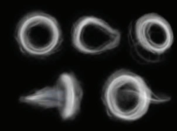
Knot theory was never actually intended for certain branches of quantum fields or even mathematics, rather chemistry. Where in the latter half of the 19th century, Lord Kelvin suggested that atoms would consist of knotted rings of an ether like substance where different elements had different knots. This idea came to mind after watching smoke rings floating in the air, as was the usual from the pipes which were commonplace at the time. This theory would hopefully enlighten scientists on how different elements would absorb and emit light at different wavelengths. The early proof, in 1860, came from the spectrum lines visible from the element. Spectral lines are produced as each element has its own energy, and will produce photons of distinct energy

levels which appear as colours at distinct levels. Knot theory would hopefully explain why each element will have a unique ‘fingerprint’ of spectral lines. Sadly while these theoretical possibilities sounded logical, when tested these did not end up being the case. Even though he was not first person to take a leap forward into the mathematics of knots, Kelvin was the first person to aim to tabulate these findings.Sil06

Gauss Code

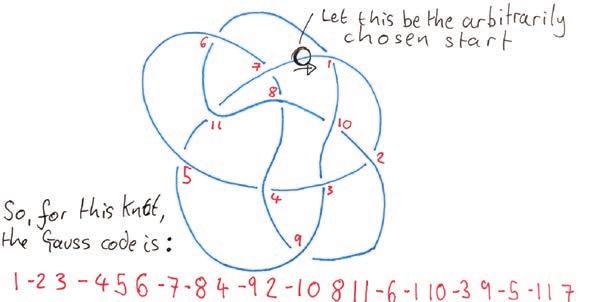
The first person to make progress into the mathematics behind knots was Carl Friedrich Gauss in the early 1800’s. His early theories involved the following idea.

1. Arbitrarily choosing a point on a line.

2. Imagine you are walking the knot, labelling the first crossing (the point on a knot where two strands overlap) as 1, and any future crossings you reach as 2, 3, and so on, until you get back to where you start.

3. To record the Gauss code of the knot, you simply walk the knot again, this time noting down each crossing you reach, and if your strand goes over another, note down as the positive value of the crossing, and if it goes under another, it will be recorded as negative.

An example of the Gauss code can be seen in figure 2: Extended Gauss Code.

Figure 1: Smoke rings simulating knotted ether

Lord Kelvin Vortex Atom

taken place. This creates a new and more complex knot which combines the properties of the two individual knots.

All of the Prime knots can be seen below up to the seventh crossing but if you expand this list up to the sixteenth crossing you get 1701936 different prime knots. Lic81

However, Gauss never realised the potential this branch of mathematics he had discovered held and left his research with the extended Gauss code, which was able to further describe the construction of the knot by giving the positive and negative values depending on the nature of the crossing. The nature of the crossing being if when it passes underneath or over, whether or ‘knot’ it is a right handed crossing or a left handed one. This is shown in figure 3.

3: Depicting the two forms of crossings

This can lead to a more complex code for each given knot but with each code being more complex, the benefit gained is when analysing the code, it is possible to recreate the knot to a more exact form than with the simple Gauss code.Bre06

KEY DEFINITIONS

As Knot theory developed, certain key concepts were definied, namely being prime knots and variants which are still key to modern day developments in knot theory.

Prime Knots

A prime knot holds a status similar to prime numbers.

This is a knot which can not be decomposed into any simpler knots the knot sum process. The knot sum process is where you take to knots and by cutting each knot open at any point and then joining the ends to any other knot where the same process has

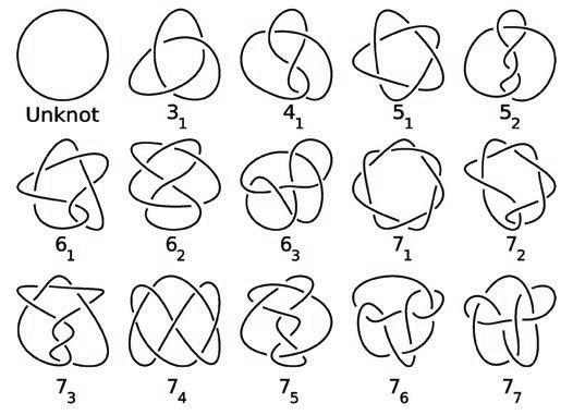
Figure 4:

Variants

Variants are distinct shapes that one can create by distorting a particular knot in it’s form. For example, take any general knot, for instance the trefoil. By altering the way it twists or loops, or even adding in new twists and loops, you might be able to get the same basic knot in a different form. Many these variants can look drastically different, though they are all are based on topologically the same starting knot.

One other way this is similar is in fractions where 2/3 is the same as 4/6. These are variants of each other but we know that these two fractions are the same. This is the same principal in Knot theory where the unknot is the same as the Goeritz unkot while looking completely different.Wu92

For another example, each time you take any simple knot and add just one extra loop or twist, you generate a new variant of that original knot. Variants, in this way, give tools by which mathematicians understand all possible configurations of the shape a single knot can assume. This teaches mathematicians about the fundamental properties of knots and how they compare to each other.PW10

Figure 2: Example of a knot with it’s Gauss code

Figure

Showing all Prime Knots up to the 7 th crossing

REIDEMEISTER MOVES

In 1927, the basis of knot theory as its known today was discovered. Kurt Reidemeister wanted to prove that knots do exist that are distinct from the unknot. The unknot can be thought of as a single loop with no crossovers or alternatively a slack elastic band. He went on to develop a series of 3 moves which could be completed without changing the underlying topology of the knot. These moves are local transformations which are as follows:

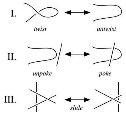
Figure 7: Depicting the 3 Reidemeister moves

With the development of these moves, he was able to identify whether a knot is distinct from another knot. However at this stage, this required many hours of trial and error completing the calculations.

Reidemeister used these moves he had discovered hich do not change the underlying topology of the knot to rigorously prove that there were knots that were different to the unknot. Which may sound trivial but I opened up the world of knot theory for future mathematicians to develop.Tra83

TRICOLOURABILITY

Theories began developing from knot diagrams to other ways to differentiate knots. A knot diagram being the simplified representation of a knot drawn on a single plane and each knot strand is represented as continuous curves. The key rule of tricolourability is that no two sections that share a common edge should be assigned the same colour. A section of a knot being from where if you follow the knot from where it goes under the last crossing to the next point it goes under the next crossing, as shown in figure 5 where each section of the knot is coloured using red, green, and blue.Alm12

There are knots that are not tricolourable, such as the figure-eight knot. The reason tricolourability is so useful, is that this process can be used to serve as a variant for distinguishing distinct knots. This is because the Reidemeister moves, which as stated earlier, do not change the topology of the knot. And as each of the 3 Reidemeister moves are tricolourable, if the prime knot is tricolourable, all other variants will be tricolourable as well.BH15

Figure 5: The Goeritz unknot

Figure 6: An example of the unknot and another of the unknot variants

Figure 8: Example of a tricolourable trefoil

This makes tricolourability a very useful technique for comparing knots. This simple process aids in categorizing and developing the subject of knot theory. While also allowing people to easily see a visual difference without having to do complicated mathematics.Azr12

Figure 9: Example of a non-tricolourable figure of eight knot

JONES POLYNOMIAL

The Jones polynomial is a relatively new discovery in the realm of knot theory which adds a unique polynomial number to each knot or link, from which they are sorted into different categories. The polynomial was invented by Vaughan Jones in the 1980s and has become one of the most powerful tools in modern knot theory.Jon05 To understand the Jones Polynomial better, It’s important to explain what a knot diagram is again. A diagram is nothing but a series of crossings: at each crossing, one of the ‘threads’ can go over or under another ‘thread’. With this at our disposal we can then compute the Jones polynomial for the given knot. For one of the simplest knots, the trefoil, where the given polynomial is V(t). Which is V(t) = t² - t + 1, where t is simply a representation of the knot diagram. However this is not the important part of the equation, what matters are the powers which show the crossings. If we compare this to the unknot

which has a Jones polynomial of V(t) = 1, comparing V(t) = t² - t + 1 to V(t) = 1, we can clearly see that they are different.Jon14 This is the power of the Jones Polynomial, it is able to tell the difference between things that, from an initial glance, look the exact same. But have different Jones polynomials. It is likely that two knots with the same Jones polynomial are the same topological knot, but further checks are needed to be certain. But to summarise, imagine the Jones polynomial as a signature for knots which is each individual polynomial. This allows mathematicians to tell the knots apart and to examine them more easily.Big02

7 MODERN USES

7.1 Biological DNA

Now we can somewhat understand the way a knot is created and categorised, how could what seems to be a purely theoretical concept be able to save a life?

If we take a look at biology, specifically at the structure of DNA, the classic double helix. To create human life, the amount of data required to be stored on DNA is massive. Requiring these strands of DNA to be up to 2m long. To sustain human life, this DNA needs to be constantly produced and as it is produced these long strands inevitably get knotted up. Take any cables, when left in a box, will inevitably get knotted up. Developments have been made recently where we are now able to autonomously analyse and unknot a knot using a robot. This uses the principles of knot theory to predict what will happen when a certain action is performed.VSK+22 Now using these principles modern scientists are able to analyse strands of DNA and where required, unknot segments and in other cases create knots. By recreating natural knots in the DNA which may have been broken certain functions will be restored. As the shape is important for binding sites in the cell, damaged DNA may be life threatening and this new research can help save lives by fixing this DNA or creating new strands.LJ15

7.2 Quantum Computing

Quantum computing is what the world is moving towards as we require computers to handle larger and more complicated questions. Quantum computing is based on quibits that can coexist in many steps allowing these computers to deal with many complex problems at the same time. This technology is currently used for breaking encryption methods. There are two big problems, namely the fact that it is very expensive and there is a lot of hardware required but also that quibits are easily disturbed in the environment. Col06

The Topological computer aims to solve these problems using braided anyons. This significantly reduces the likelihood of errors forming and the calculations can be done faster using polynomial time not euclidean time. However precise manipulation is required when dealing with anyons, as only recently was there experiments proving they exist. However further developments are needed to understand the structure and how to layer them in computers. MMM+18

By using knot theory in the building of quantum computers we get the fact that: knot theory is being used to build computers which are used to find new variants for knot theory, developing the subject while making technological advances.

Figure 10: Example of a knotted loop of DNA

Figure 11: An example of a knot which can be braided by anyons to be used in a topological quantum computer

SUMMARY

Knots are more than just objects in a physical world, but instead concern a complicated study in both mathematics and science. From initial hypotheses by people like Kelvin and Gauss has developed into this sophisticated discipline which is knot theory. The tools we need are given to us by the work of the Jones polynomial and the Reidemeister moves allowing us to classify and manipulate knots.

From this abstract branch of mathematics modern uses span into many areas for example biology and chemistry. But majorly quantum computing where knot theory is the key in developing more advanced ideas. As more research develops, further links with knot theory are being made and why the study of knot theory is so important to our future.

REFERENCES

1. [Alm12] Manuela Almeida. Knot theory Estados Unidos, 2012.

2. [Azr12] M Azram. Knots and colorability Australian Journal of Basic and Applied Sciences, 6(2):76–79, 2012.

3. [BH15] Danielle Brushaber and McKenzie Hennen. Knot tricolorability. 2015.

4. [Big02] Stephen Bigelow. A homological definition of the jones polynomial Geometry & Topology Monographs, 4:2941, 2002.

5. [Bir93] Joan S Birman. New points of view in knot theory. Bulletin of the American Mathematical Society, 28(2):253–287, 1993.

6. [Bre06] Felix Breuer. Gauss codes and thrackles PhD thesis, Citeseer, 2006.

7. [Col06] Graham P Collins. Computing with quantum knots. Scientific American, 294(4):56–63, 2006.

8. [DF87] MJ Dunwoody and RA Fenn. On the finiteness of higher knot sums Topology, 26(3):337–343, 1987.

9. [Jon05] Vaughan F.R. Jones. The jones polynomial. University of California, 2005.

10. [Jon14] Vaughan Jones. The jones polynomial for dummies. University of California Berkley, 2014.

11. [Lic81] WB Lickorish. Prime knots and tangles Transactions of the American Mathematical Society, 267(1):321–332, 1981.

12. [LJ15] Nicole CH Lim and Sophie E Jackson. Molecular knots in biology and chemistry. Journal of Physics: Condensed Matter, 27(35):354101, 2015.

13. [Man18] Vassily Olegovich Manturov. Knot theory. CRC press, 2018.

14. [MK96] Kunio Murasugi and Bohdan Kurpita. Knot theory and its applications. Springer, 1996.

15. [MMM+18] D Melnikov, A Mironov, S Mironov, A Morozov, and An Morozov. Towards topological quantum computer Nuclear Physics B, 926:491–508, 2018.

16. [PW10] Peter Pagin and Dag Westerst˚ahl. Compositionality i: Definitions and variants. Philosophy Compass, 5(3):250–264, 2010.

17. [Sil06] Daniel S Silver. Knot theory’s odd origins: The modern study of knots grew out an attempt by three 19th-century scottish physicists to apply knot theory to fundamental questions about the universe. American Scientist, 94(2):158–165, 2006.

18. [Tra83] Bruce Trace. On the reidemeister moves of a classical knot. Proceedings of the American Mathematical Society, 89(4):722–724, 1983.

19. [VSK+22] Vainavi Viswanath, Kaushik Shivakumar, Justin Kerr, Brijen Thananjeyan, Ellen Novoseller, Jeffrey Ichnowski, Alejandro Escontrela, Michael Laskey, Joseph E Gonzalez, and Ken Goldberg. Autonomously untangling long cables. arXiv preprint arXiv:2207.07813, 2022.

20. [Wu92] FY Wu. Knot theory and statistical mechanics. Reviews of modern physics, 64(4):1099, 1992.

STEM

DANIEL HUGHES

BAND STRUCTURE ANALYSIS

Analysing the band structure of bulk and monolayer Transition Metal Dichalcogenides including Janus MXY structures

This Original Research in Science (ORIS) project was short-listed for the ILA/ ORIS Presentation Evening.

INTRODUCTION

Crystal Structures

A crystal is a solid material in which the component atoms are arranged in a definite, periodic pattern. A solid is crystalline if it has long-range order - once the positions of an atom and its neighbours are known at one point, the place of each atom is known precisely throughout the crystal. A basic concept in crystal structures is the unit cell. It is the smallest unit of volume that permits identical cells to be stacked together to fill all space. By repeating the pattern of the unit cell over and over in all directions, the entire crystal can be constructed. This regular repetition of the unit cell makes the crystal

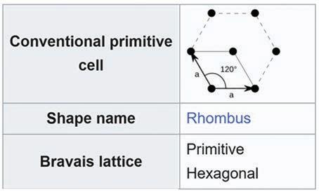
a periodic structure. The structure of all crystals can be described in terms of a lattice, with each atom or group of atoms replaced by a point in space forming a crystal lattice with the same geometrical properties as the crystal. In 1848, the French physicist, Auguste Bravais, identified 5 lattices from which all possible cases in 2-dimensional space can be represented and 14 possible lattice structures in 3-dimensional space. A fundamental aspect of any Bravais lattice is that, for any choice of direction, the lattice appears exactly the same from each of the discrete lattice points when looking in that chosen direction.

Mathematically, the unit cells of a Bravais Lattice are specified according to six lattice parameters which are the relative lengths of the cell edges (a, b, c) and the angles between them (α, β, γ), where α is the angle between b and c, β is the angle between a and c, and γ is the angle between a and b. The lengths of the cell edges are typically measured in angstrom (Å) - a unit of length that is equal to one ten-billionth of a meter, or 0.1 nanometres.

Band Theory

Band Theory is a fundamental model in solid-state physics that has been developed to describe the behaviour of electrons in a periodic potential, such as that found in a crystal lattice, and the electronic properties of crystalline materials.

In an atom, electrons occupy discrete energy levels, often referred to as atomic orbitals (in the real space an orbital corresponds to regions of space around an atom where there is a high probability of finding an electron). Band theory extends this concept to explain the behaviour of electrons in a solid material and it is most commonly applied to a crystalline solid. When atoms come together to form a solid, their atomic orbitals overlap. This overlap causes the energy levels of the orbitals to split, forming a continuous band of energy levels. These bands are called energy bands.

The arrangement of these bands and their occupation by electrons (which occupy the levels starting from the lowest energy but only two electrons per one state) determine the electrical conductivity of a material:

● Conduction band: This is the highest-energy empty or partially filled band. If there are available energy states in this band, electrons can move freely, making the material a good conductor.

● Valence band: This is the lowest-energy band filled with electrons.

● Band gap: This is the energy gap (if any) between the valence and conduction bands. If the valence band is fully occupied, the conduction band is completely empty and the energy gap is large, the material is an insulator. If the gap is smaller, the material is a semiconductor. If there is no energy gap and the highest-energy occupied band is partially filled, the material is a metal.

3D views of the crystal TaS₂ (mp-1984) taken from The Materials Project

TMDs

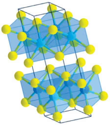
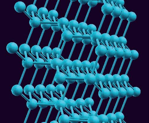
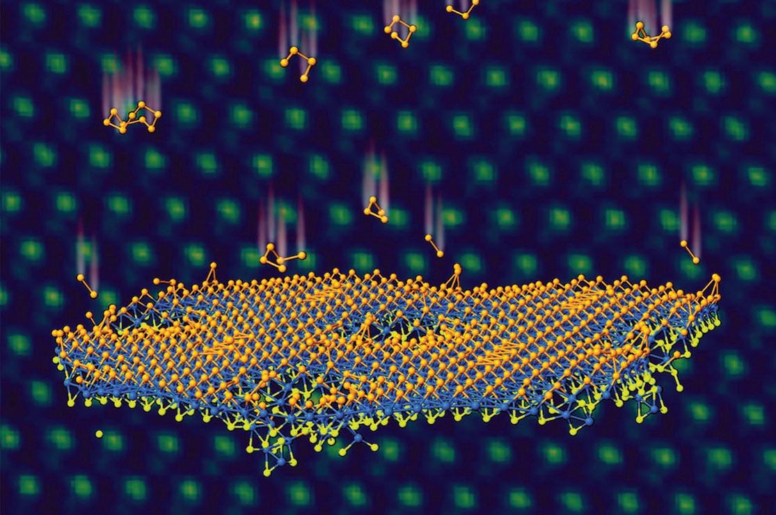
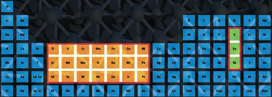
Transition metal dichalcogenides (TMDs) are a class of layered materials with regular crystal structures, that can be described by the general formula MX2, in which a layer of transition metal (M) is sandwiched between two layers of chalcogen atoms (X). Such 'sandwiches' are then stacked on top of each other, analogous to the stacking of graphene layers in graphite. TMDs can be found as bulk multilayer 3D materials (like graphite) or 2D mono-layer materials (like graphene). This research explores the properties of both of these forms.

TMDs have garnered interest because as a group they display a wide range of electronic properties (for example, some are semiconductors and some are metals; most are superconductors at sufficiently low temperatures), leading to a large potential range of applications including energy harvesting, sensing and nano-scale actuators.

Phases

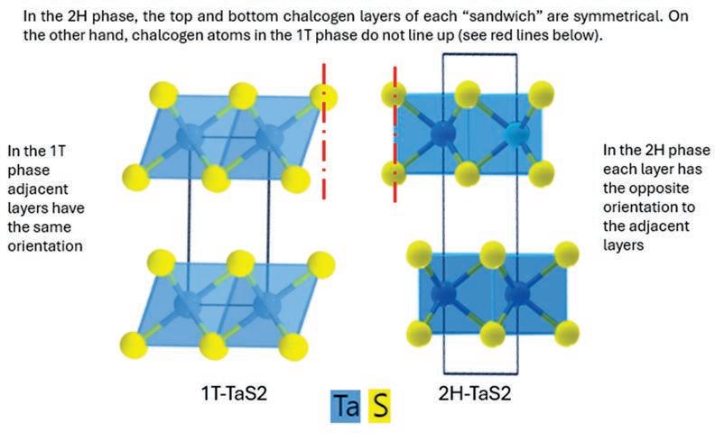
TMDs can also exist in several crystallographic phases, notably the 2H and 1T phases which this research focuses on. Whilst they have the same chemical formula, phases differ by the way in which atoms are arranged within and between layers. Just like with liquid water and ice, in given conditions (e.g pressure, temperature), one phase is the most stable although

several phases can coexist in the same crystal. For comparison, consider graphite and diamond which are different crystalline phases of carbon: both can exist in ambient conditions although graphite is the more stable phase.

Both phases consist of layers of transition metals and chalcogens. In each layer, atoms of the same element are arranged in equilateral triangles and each layer of transition metals is sandwiched between two layers of chalcogens. In the 2H phase, the top and bottom chalcogen layers of each 'sandwich' are oriented in the same direction relative to each other. When a 3D model of the 'sandwich' is viewed in the x or y direction the chalcogen atoms appear to be aligned with each other such that a line drawn parallel to the z axis of the unit cell would pass through both.

On the other hand, chalcogen atoms in the 1T phase do not line up when viewed in the x or y direction. Instead, the topmost and bottommost chalcogen layers of the 'sandwich' are oriented in the opposite directions (rotated by 180 degrees which swaps the orientation of the equilateral triangles). Additionally, in the 2H phase, each 'sandwich' is stacked with the opposite orientation to the previous one whereas each 'sandwich' in the 1T phase is stacked with the same orientation.

Source: ball and stick model from materials project

In the 2H phase, each layer has the opposite orientation to the adjacent layers. Therefore, the smallest repeatable unit must contain two layers (as opposed to the 1T unit cell which has one layer). As a result the unit cell of the 2H phase consists of 6 atoms whereas the unit cell of the 1T phase consists of 3 atoms and there are double the number of the bands between them.

Materials and Analysis

In this research I will investigate TaS2 and TaSe2. These materials both have interesting electronic and optical properties and under certain conditions can exhibit superconductivity. They are being considered for a range of uses; currently their most common use is in the production of lithium-ion batteries where they can increase their efficiency and lifetime.

I will also investigate MoS2 which is the most widely used transition metal dichalcogenide (TMD) material because it is relatively abundant and can be produced at a relatively low cost. MoS2 has found applications in fields like electronics, energy storage, catalysis, and sensors. Its layered structure allows the layers to slide over each other with minimal friction, making it an excellent material for reducing wear and tear in mechanical components and it is widely used as a lubricant in the automative and aviation industries.

Furthermore, I also explore a subset of TMDs known as Janus MXY structures (the name refers to the

Roman god Janus with two faces). In particular, I will be analysing the structure of the hitherto not yet synthesised Janus structure TaSeS and comparing its electronic properties with the aforementioned materials under the same conditions. The Janus MXY structure differs from other TMDs in that the top and bottommost layers of the sandwich consist of different chalcogens. For instance, in TaSeS one layer consists of the chalcogen selenium and the other of sulphur. In such Janus materials, the differences in the number of electrons in S and Se lead to the appearance of electric polarization and piezoelectricity.

I hypothesise that the properties of TaSeS would be well approximated by an average of TaSe2 and TaS2.

Aims:

The aim of this research project was twofold;

1. To model the band structures of several transition metal dichalcogenides (TaS2, TaSe2 and MoS2) to compare the impact of differences in symmetry, chemistry and dimensionality on the electronic properties of a material.

2. To predict the possible crystal structure and electronic bands of a new, not yet synthesized material, Janus TaSeS to analyse the impact of mixing of S and Se atoms.

I will make comparisons between:

● Symmetry: materials with the same chemistry but different phase

● Chemistry: the same phase but different chemistry’

● Dimensionality: the same phase and chemistry but different dimensionality (three-dimensional bulk material vs a single, effectively two-dimensional, 'sandwich').

In order to analyse the electronic properties of these materials, I will plot a band structure graph describing the energy levels electrons can take with energy on the y-axis and momentum on the x-axis. In its simplest form, the band structure of a material can be thought of as consisting of a block of valence and conduction bands separated at the Fermi energy and perhaps also by a band gap (as illustrated in the diagram).

“ The band structure of a material can be thought of as

consisting of a block of valence and conduction bands separated at the Fermi energy and perhaps also by a band gap.

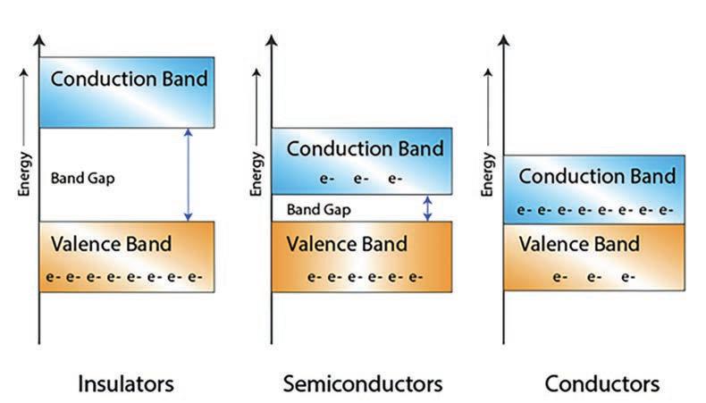
At zero Kelvin the valence band is filled, and the conduction band is empty, however, as more energy is added some electrons may be promoted to the conduction band depending on the size of the band gap. If there is no band gap the material is metallic, and many electrons are promoted to the conduction band even if little energy is provided. If the band gap is sufficiently small, then the material is a semiconductor, and some electrons are promoted to the conduction band using relatively little energy. If the gap is too large, electrons can only be promoted to the conduction band moderate energy if moderate energy is provided and the material is an insulator.

METHOD

Learning

During the first phase of the project, I spent some time reading background material and learning to use Quantum Espresso (QE). My Project Sponsor, Dr Marcin Mucha-Kruczyński, provided me with a number of articles about research projects relating to TMDs which provided an excellent background to the project, and I also referred to a number of other texts and online resources. A study of the mathematics underlying Band Theory, given its complexity, was outside the scope of this project.

QE is an open-source collection of programs which was developed by a large international collaboration of researchers, primarily from institutions in Italy and the United States. It is based on Density Functional Theory and uses plane waves together with so-called pseudopotentials to enable calculations of the electronic structures of materials, simulation of complex molecular systems and prediction of material properties. DFT is a computational quantum mechanical modelling method grounded in the Schrödinger equation, which is itself the fundamental equation of Quantum Mechanics that describes the wave-like behaviour of atomic and sub-atomic particles.

QE makes it possible to carry out very complicated calculations within a reasonable amount of time without access to significant computing power. In order to be able to run QE on my laptop I created a Linux Virtual Machine (an independent space on my Windows-based computer that would run the Linux Ubuntu operating system) and downloaded the Quantum Mobile VM image (which had QE preinstalled) into this VM.

Initially I learned to run pre-prepared material files available from online tutorials to gain familiarity with the software before moving on to learn how to write these files myself and where to obtain the input data.

Following the preparation phase I undertook the field work during a two-week trip to the University of Bath. I met regularly with Dr Marcin Mucha-Kruczyński during this period to discuss progress and learning points that came up as the project progressed.

Finding Data

The first stage for each material whose band structure I was plotting was to find the relevant information about the crystal structure and unit cell of that material. The data I needed to carry out the calculations in QE were:

● the Bravais lattice index,

● cell constants a and c,

● the number of atoms in the unit cell, and

● atomic positions within the unit cell.

Since all the TMDs I researched had hexagonal lattice structure, their unit cells were all rhombohedral in shape and as such the only cell constants I needed were a and c since the a and b side lengths are the same.

Source: Wikipedia

I also needed to find a pseudopotential file for each element involved. A pseudopotential is used as an approximation that provides a simplified description of complex systems; only the chemically active valence electrons (those in the outermost shell which interact with other atoms) are dealt with explicitly, while the core electrons are 'frozen', being considered together with the nuclei.

In selecting the type of pseudopotential to use I opted for scalar relativistic ones which, unlike the full relativistic versions, do not take account of the impact of electron spin. This simplification reduced the time taken to run each calculation on my laptop. I also tried to run some calculations using full relativistic pseudopotentials, however, these calculations took too long to provide a complete set of results within the time frame of the project. Additionally, using scalar relativistic pseudopotentials meant that it was quicker and easier to debug the input files.

I was able to find most of the data set out above at The Materials Project website. The Materials Project is a multi-institution, multi-national effort that uses supercomputers (including, for example, the National Energy Research Scientific Computing Center in Berkeley, California which is part of the U.S. Department of Energy) to compute the properties of all inorganic materials and provide the data for researchers free of charge. The aim of the project is to reduce the time needed to invent new materials through focusing laboratory work on compounds that already show the most promise computationally.

The use of supercomputers enables the prediction of many properties of new materials before those materials are ever synthesised in the lab. However, the data I needed for 2H-TaSeS (which has not yet been synthesised in the lab) was not yet available in The Materials Project so I had to carry out an additional calculation for this material as explained below.

Calculating the Fermi Energy

Fermi energy is a fundamental quantity in solid-state physics that represents the highest energy level occupied by an electron at absolute zero temperature. In band theory, the position of the Fermi energy relative to the band structure determines whether a material is a metal, insulator, or semiconductor.

In order to calculate the Fermi energy for each material I needed to create and run the SCF file in QE.

Self-Consistent Field (SCF) is a computational method used in QE to approximate the electronic structure of molecules and atoms.

Key input data for this included:

● the Bravais lattice index (which is 4 for hexagonal structures),

● cell constants a and c in Angstrom,

● atomic positions (in Crystal Coordinates),

● number of atoms.

I also needed to specify which elements made up the TMD and for each element I specified its atomic mass as well as a relevant pseudo-potential file. The SCF calculation also required several other parameters not directly related to the TMD itself. For instance, I had to set the Kinetic Energy Cutoff for wavefunctions. Kinetic Energy Cutoff determines the maximum kinetic energy of the plane waves used to represent the electronic wavefunctions. Selecting a higher value generally leads to more accurate results but also increases the computational cost significantly.

I tested a range of values for this cutoff and chose a value of 680 eV because it provided an optimal trade-off between accuracy of results and length of calculation time.

Having created the SCF input file for each material, I then inputted it to Pw.x to run the SCF calculation. Pw.x is one of the core programme modules in QE. It primarily performs plane-wave SCF calculations by iteratively solving the Kohn-Sham equations to determine the ground-state electronic structure of a system. The Kohn-Sham equations are a set of equations used to simplify the complex problem of understanding how electrons behave in atoms and molecules. Ground-state electronic structure refers to the arrangement of electrons in a system at its lowest possible energy state (its most stable state). As part of the output, Pw.x provided a value for the Fermi energy of each material.

Converting 3D Bulk Input to 2D Monolayer Input

Since Quantum Espresso is designed to run calculations for three-dimensional materials by default, in order to model monolayers, I had to adjust the parameters of the unit cell to provide an approximation for a monolayer within the multilayer simulation. I did this by increasing the cell constant 'c' which lengthened the ‘z’ axis of the unit cell, thus increasing the distance between layers. As the distance between layers increases, the interaction between them decreases, so by sufficiently increasing c I could minimise the interaction between layers and in effect simulate the properties of a single monolayer.

However, since I was using relative coordinates for the atomic positions within the unit cell, this meant that the absolute distance between the atoms in each layer also increased which would cause erroneous results. To fix this, I needed to scale z positions of the atoms within the unit cell so that the absolute distance between the atoms within each layer stayed the same. Since I was doubling the value of c for each monolayer calculation, this involved halving the z coordinates of the atomic positions and applying an offset where appropriate. This ensured that the layer itself would remain unchanged even though the distance between the layers increased.

“ As the distance between layers increases, the interaction between them decreases, so by sufficiently increasing c I could minimise the interaction between layers and in effect simulate the properties of a single monolayer.

Calculating the Atomic Structure of 2H-TaSeS

The input data regarding the atomic structure required to calculate the Fermi energy (as outlined above) was available in The Material Projects for each of the materials I studied other than 2H-TaSeS. TaSeS is a material which has not yet been synthesised in a laboratory.

In order to calculate the atomic structure of 2H-TaSeS I used the VC-relax calculation in QE which adjusts the size and shape of the unit cell to find the most energetically favourable configuration. VC-relax can be used to determine the equilibrium lattice parameters and atomic positions of a material:

1. Initial Structure: The calculation starts with an initial guess for the unit cell parameters.

2. Relaxation: The software iteratively adjusts the volume and cell parameters while minimizing the total energy of the system.

3. Convergence: The calculation continues until a converged structure is reached, meaning the forces on the atoms are negligible and the lowest energy (and most stable) configuration of the structure has been found.

Band structure calculations

Before performing the band structure calculations, I first had to determine a set of k-points that I would keep the same throughout my calculations to ensure comparable band structure plots for different materials.

To perform calculations efficiently, a finite set of special points in the Brillouin zone, known as k-points, are sampled rather than calculating the electronic structure at every point in the Brillouin zone.

Since I was going to compare the differences between the bulk and monolayer forms of each TMD, I decided to use 2D k-points only (as the mono-layer forms have no 3D k-points), setting the z component (which represents the third dimension) of each to zero.

To generate a set of k-points for the calculations, I used the SeeK path tool from the Materials Cloud website (an open source resource designed for materials researchers) to help visualise the Brillouin zone and generate a range of values connecting the Γ (Gamma), M and K high-symmetry points (relevant to the 2D hexagonal lattice).

● Γ (Gamma): Centre of the Brillouin zone

● K: Located at the corners of the hexagon

● M: Midpoints of the edges of the hexagon

● Having selected a set of k-points using the Materials Cloud tool, I then created and ran a Python script to plot them on a graph to provide a visual check (against the expected output shape that was sketched out by my Project Sponsor) before confirming my selection.

I then created a new input file with similar inputs to the SCF input file as well as the specific set of k-points. I then ran this file using Pw.x specifying that a band structure calculation should commence.

Using the output files from these calculations I then ran the Bands.x QE module to produce band structure data in format that could be plotted using the Plotband.x QE module.

Project Timeframe

Prior to the start of the fieldwork I had two Teams calls with my Project Sponsor, Dr Marcin Mucha-Kruczyński, to discuss the scope of the project and some of the background to the underlying key physics concepts I would be working with.

During the first phase of the project prior to starting the fieldwork, I spent some time reading background material and learning to use Quantum Espresso (QE). This preparation phase was spread over a number of months but in total encompassed around two week’s work on a full time basis.

Following the preparation phase, I undertook the field work during a two-week trip to the University of Bath (29 July to 9 August 2024). I met regularly with Dr Marcin Mucha-Kruczyński during this period to discuss progress and learning points that came up as the project progressed.

FINAL RESULTS AND CONCLUSION

For each material, I plotted a band structure along the path connecting the high-symmetry points Gamma, M, K and returning back to Gamma. I set the Fermi energy as the 'zero' reference value for each graph, plotting +/-2eV as the range of the y-axis to provide a closer view of the bands around the Fermi energy. This is the energy range relevant to the physics of electronic transport.

In these graphs, the conduction bands are at the top and may cross the Fermi energy (indicated with a horizontal dashed line). The fact that they do so indicates that the material is a conductor. The valence bands are in the lower half of the graph. I produced 16 band structure graphs showing the 1T and 2H phases in both 2D (monolayer) and 3D (bulk) form for each TMD that I investigated.

The number of the bands, how close together they are, whether the bands are steep or flat, the number of times a conduction band crosses the Fermi energy are all examples of factors which provide information about the electronic properties of a material. Consider, for example, applying a voltage to a material which provides energy to the electrons. However, they can only take advantage of this if there are higher energy states that they can move into. Therefore, knowledge of the band structure near the Fermi energy level is crucial for modelling or predicting the properties such as electronic transport of a material. A detailed consideration and measurement of the impact of these factors is beyond the scope of this project. In the analysis below I have made high level reference to these factors where they are relevant but have largely focused my comments on the interaction of the conduction bands with the Fermi energy level.

Impact of Change in Phase

In both the 1T and 2H phases of the 2D forms of TaSe2, TaS2 and TaSeS (the Janus material) one conduction band crossed the Fermi energy line indicating that they are all conductors and the change in phase did not impact this core characteristic. The graphs of the 2D forms do show a degree of similarity, however, the slope of the conduction band is steeper in the 1T phase whilst in the 2H phase the conduction band crosses or touches the Fermi energy level one additional time. Overall, a larger part of the conduction band seems to be occupied (that is, lies below the Fermi energy) in the 1T phase than in the 2H phase.

“ In my analysis of the results, I observed that changing the chalcogen atom of the TMD has less impact than changing the metal atom on the electronic band structure of the TMD.

Both the 1T and 2H 3D or bulk forms of TaSe2, TaS2 and TaSeS are conductors. However, in the 2H phase two bands cross the Fermi energy level whereas only one band crosses it in the 1T phase. This difference was probably due to the number of layers in the unit cell of the 2H phase, two, as compared to one for the 1T phase. Therefore, the number of atoms considered in the 2H calculation was double that considered in the 1T band calculation thus doubling the number of bands plotted.

Whilst the TaSe2, TaS2 and TaSeS TMDs I investigated are all metallic in both phases, MoS2 changed from a conductor in the 1T phase (with three bands crossing the Fermi energy level) to a semiconductor in the 2H phase with no bands crossed the Fermi energy and a small band gap. This was the same in both bulk and monolayer forms of MoS2.

Impact of Change in Chemistry

In their 1T phases and in both monolayer and bulk form, TaSe2, TaS2 and TaSeS were very similar with both one band crossing the Fermi energy level with a similar shape. This suggests that changing the chalcogen atom has little impact on the electronic band structure in the 1T phase.

More differences could be seen within the 1T phase when the metal was changed - from 2D 1T-TaS2 to 2D 1T-MoS2. Whilst both are conductors, in 1T-MoS2 three bands cross the Fermi energy level six times, whereas in 1T-TaS2 one band crosses twice. This suggests that in the 1T phase, changing the metal making up the TMD had a more significant impact on its’ electronic structure than changing the chalcogen. In the 2H phase of TaSe2, TaS2 and TaSeS changing the chalcogen also has a limited impact and the bands remain similar for the three materials. However, in 2D TaSeS 2D the conduction band crosses the Fermi energy level in between the K and Gamma high-symmetry points (whereas in the other two materials it only touches it) and in 3D TaSeS the 'top' conduction band only crosses twice (in the other two materials the top line crosses four times).

Changing the metal in the 2H phase (e.g 2H-TaS2 2D to 2H-MoS2 2D) had an even more significant than in the 1T phase changing the material from a metal to a semi-conductor. The greater impact of changing the transition metal than the chalcogen is because the former modifies the number of valence electrons involved (requires moving horizontally in the periodic table). This changes the number of electrons that must be distributed in the bands and so shifts the position of the Fermi energy level. In contrast, the chalcogen atoms have the same number of valence electrons (they are in the same column of the periodic table) so little change is observed.

The greater impact of changing the transition metal than the chalcogen is due to the fact that changing the former modifies the number of valence electrons

involved (requires moving horizontally in the table of elements). This in turn changes the number of electrons that have to be distributed in the bands and so shifts the position of the Fermi energy. In contrast, the chalcogen atoms have the same number of valence electrons (are in the same column of the table of elements) and so little change is observed.

Impact of Change in Dimensionality

When comparing the 3D bulk and 2D monolayer band structure graphs for the 1T phase of TaS2, TaSe2 and TaSeS, there is little variation in the bands crossing the Fermi energy level. However, for the 2H phase, the number of bands crossing the Fermi energy in the monolayer form is halved: the two bands crossing the Fermi energy level for the bulk form are replaced by a single band that appears to be roughly an average of the two. This is because the 2H unit cell in the 3D form consists of two layers whereas the monolayer calculation was adjusted to reduce the interaction between layers, simulating the properties of a single layer only.

In its bulk form, the conduction band minimum of 2H-MoS2 is approximately halfway between the K and Gamma high-symmetry points and the valence band maximum is at the Gamma point, resulting in a band gap of approximately 1.1eV. The monolayer form of MoS2 differs noticeably from its bulk form: whilst the valence band maximum is still at the Gamma point, it is at a lower energy than in the bulk form. Furthermore, the shape of the conduction band is different such that the global minimum is at the K high-symmetry point resulting in a larger band gap of approximately 1.5eV.

CONCLUSION

In my analysis of the results, I observed that changing the chalcogen atom of the TMD has less impact than changing the metal atom on the electronic band structure of the TMD. I also observed that changing phase impacts the properties of TMDs differently depending on their chemical structure as there was a significant change in MoS2 but not in TaS2. Additionally, changing dimensionality did not have a large impact in the 1T phase but had a larger impact in the 2H phase due to the presence of two layers within the unit cell.

Overall, I can conclude that the mixing of S and Se atoms to produce the hypothetical Janus material TaSeS results in a material whose electronic band structure can be approximated by a combination of TaSe2 and TaS2 with a smooth change between the properties of the two rather than a sudden and more drastic change in band structure.

ABSTRACT

Transition metal dichalcogenides are a group of materials in which a layer of transition metals is sandwiched between two layers of chalcogen atoms. Such 'sandwiches' are then stacked on top of each other. I use the multi-purpose nanoscale materials simulation software Quantum Espresso to model the band structures of several transition metal dichalcogenides: TaS2 (tantalum disulphide), TaSe2 (tantalum diselenide) and MoS2 (molybdenum disulphide). This selection of materials allows me to compare the impact of differences in symmetry, chemistry and dimensionality on the electronic properties of a material. I also use Quantum Espresso to predict the possible crystal structure and electronic bands of a new, as of yet not synthesized material, Janus TaSeS (tantalum selenium sulphide), in which in each sandwich one chalcogen layer consists of S atoms and another of Se. My findings show that the mixing of S and Se atoms to produce TaSeS results in a material with properties well approximated by the average of those of TaSe2 and TaS2.

ACKNOWLEDGEMENTS

I would like to thank my supervisor Dr Marcin Mucha-Kruczyński for making this ORIS project possible. His generous support, guidance and teaching allowed me to explore some fascinating aspects of condensed matter physics. The passion that he shows for the subject is inspirational and I am very grateful to have had this opportunity. I would also like to thank Mr Lau for overseeing the ORIS project and providing me with constructive advice particularly during the early stages of the project.

“

Overall, I can conclude that the mixing of S and Se atoms to produce the hypothetical Janus material TaSeS results in a material whose electronic band structure can be approximated by a combination of TaSe 2 and TaS 2 with a smooth change between the properties of the two rather than a sudden and more drastic change in band structure.

APPENDIX

Example 2D SCF file

1. &CONTROL calculation = 'scf', prefix = 'tas2', ! 2H-TaS2 2D outdir = './tmp/' pseudo_dir = '../pseudos/' verbosity = 'high' /

2. &SYSTEM

ibrav = 4 ! https://next-gen.materialsproject. org/materials/mp-1984?formula=TaS2

A = 3.34 ! lattice constant a

C = 25.10 ! c=12.55, a=3.34 angstroms -- set c=25.1 for 2D

nat = 6

ntyp = 2

ecutrho = 400

ecutwfc = 50 occupations = 'smearing' smearing = 'cold' degauss = 1.4699723600d-02 /

3. &ELECTRONS

conv_thr = 1.2000000000d-09

electron_maxstep = 80 mixing_beta = 4.0000000000d-01 /

4. ATOMIC_SPECIES

S 32.065 s_pbesol_v1.4.uspp.F.UPF

Ta 180.94788 ta_pbesol_v1.uspp.F.UPF

5. ATOMIC_POSITIONS crystal ! 2D

Ta 0.0000000000 0.0000000000 0.1250000000

Ta 0.0000000000 0.0000000000 0.6250000000

S 0.3333333300 0.6666666700 0.0632663900

S 0.3333333300 0.6666666700 0.1867336100

S 0.6666666600 0.3333333300 0.5632663900

S 0.6666666700 0.3333333300 0.6867336100

6. K_POINTS automatic 11 11 3 0 0 0

Example 3D SCF file

1. &CONTROL

calculation = 'scf', prefix = 'tas2', ! 2H-TaS2 outdir = './tmp/' pseudo_dir = '../pseudos/' verbosity = 'high' /

2. &SYSTEM

ibrav = 4! https://next-gen.materialsproject. org/materials/mp-1984?formula=TaS2 A = 3.34 ! lattice constant a C = 12.55 ! c=12.55, a=3.34 angstroms nat = 6 ntyp = 2 ecutrho = 400 ecutwfc = 50 occupations = 'smearing' smearing = 'cold' degauss = 1.4699723600d-02 /

3. &ELECTRONS

conv_thr = 1.2000000000d-09 electron_maxstep = 80 mixing_beta = 4.0000000000d-01 /

4. ATOMIC_SPECIES

S 32.065 s_pbesol_v1.4.uspp.F.UPF

Ta 180.94788 ta_pbesol_v1.uspp.F.UPF

5. ATOMIC_POSITIONS crystal

Ta 0.0000000000 0.0000000000 0.2500000000

Ta 0.0000000000 0.0000000000 0.7500000000

S 0.3333333300 0.6666666700 0.1265327800

S 0.3333333300 0.6666666700 0.3734672200

S 0.6666666600 0.3333333300 0.6265327800

S 0.6666666700 0.3333333300 0.8734672200

6. K_POINTS automatic 11 11 3 0 0 0

WHAT DOES THE FUTURE OF ASTRONAUTICAL FLIGHT LOOK LIKE?

STEM CHARLIE LOCKE

This Independent Learning Assignment (ILA) was short-listed for the ILA/ ORIS Presentation Evening

INTRODUCTION

According to NASA, the main objective of exploring space is to answer “some of the most fundamental” questions regarding our universe and ultimately answer the question of “how we can live our lives better”. An example of where their research into astronautical flight has improved the quality of our lives is with the improvements of shock-absorbing materials which allowed prosthetic limbs to be improved massively. With 45,000 people in the UK alone with prosthetic limbs, it is undisputable that the development of this branch of engineering has been invaluable.

I believe that these sorts of improvements attest to the importance of advancing research that may on the outside seem unrelated to products we use every day. I therefore believe that there is a further argument for the advancement of astronautical flight for technology that we use here on Earth. Space exploration gives us a new perspective on the Earth and is fundamental for many reasons. In the most extreme case, it could identify possible threats to our existence such as potentially colliding near-earth-objects. One day this technology may also allow us to inhabit other planets.

LIQUID ROCKET ENGINE

Now that I have made a case for the practical need for astronautical flight, I think it is chronologically important to look at the systems of propulsion for these spacecrafts. A very traditional method of rocket propulsion is a liquid such as ethanol or more recently hydrogen; used as the fuel. These rockets bring their own oxidiser allowing them to work in the airlessness of space. The reason this system has been used since the first rocket - the V-2 in 1944 (Wernher Von Braun led in 1936), is that enormous energy can be delivered in a very short amount of time. The general idea behind this engine is relatively simple compared to others that I will cover in this essay. First, fuel and stored oxidiser are pumped into a combustion chamber where they mix and burn. This produces a lot of high temperature and pressure exhaust gas. This flow of gas is then accelerated through a nozzle. The thrust is therefore produced according to Newton’s third law of motion: Thrust = mass flow rate * exit velocity + change in pressure between exit and free stream * area ratio from throat to exit.

While this may seem straightforward, the complexity comes with working out how to mix the fuel and oxidiser without blowing out the flame.

The main problem with traditional liquid rocket engines is the fact that a lot of fuel needs to be used up and this fuel is used up very quickly, usually in under 10 minutes. While this is perfect for getting straight into space, if you need to accelerate whilst in space, or change direction, you have no fuel left to do so. This problem can be in part solved by rotating detonation engines (RDEs). In a traditional liquid engine, the fuel doesn’t detonate and instead it deflagrates. This is where ignitions spread out at supersonic speeds. Notably, deflagration can be seen in objects as simple as candles. On the other hand, RDEs ignite the fuel causing an explosion by process of intense compression and heating by a supersonic shockwave. This explosion produces more thrust and in turn allows the power density to be “an order of magnitude higher than today’s devices” according to Steve Heister (Purdue University engineering professor). While this technology is extremely new, JAXA (Japan Aerospace Exploration Agency) managed to successfully test an RDE engine in space with the success of their “S-520-31 sounding rocket”. A further reason that backs up the fact that this is the future for liquid engines is the fact that more than 12 separate organisations are working on this technology, including NASA who tested an RDE engine on Earth first in January 2023 which achieved 18kN out of a desired 44kN of thrust.

Credit: NASA’s Glenn Research Centre

They then tried again in December 2023 and managed to achieve 26kN, which shows how this technology has the potential for rapid development. Despite this technology allowing rockets to burn fuel more efficiently, it doesn’t tackle the fundamental issue; you can only burn the fuel you take with you. Other issues with liquid rocket engines are that the processes they use to function are not fully understood. For example, droplet evaporation and turbulence (however this is not just a problem local to liquid rocket engines). Though these problems could be worked on, and eventually solved, the question is; is there a future for liquid engines?

I believe that while technological advancements could tackle some of these problems, it is more cost and time effective to turn to alternate propulsion systems. One such system is the ionic propulsion engine.

IONIC PROPULSION

Due to the lack of atmosphere in space, propellors are of course out of the question, and instead historically fuel must be ejected, pushing the rocket forward according to the principle of conservation of momentum. While this is an effective method for most rockets that we use today, the point of this essay is to discuss the future of astronautical flight. Since fuel needs to be burned, it needs to be carried on board. This therefore begs the question of efficiency, as I have alluded to earlier, and the rate at which this fuel needs to be burned means that a Falcon Heavy, for example, will only be able to burn its almost 400 tonnes of fuel and oxidiser for about 9.5 minutes. Scientists have therefore increasingly been researching alternative methods of propulsion, most successfully of which is the ion propulsion system. While most chemical rockets expel hot gasses at 5km/s and have an efficiency of about 35%, ion engines can eject atoms at 90km/s and have an efficiency potential of 90%.

Having made the case for the importance of ion propulsion, I will move onto discussing how it works.

Mapping of Ion Thruster

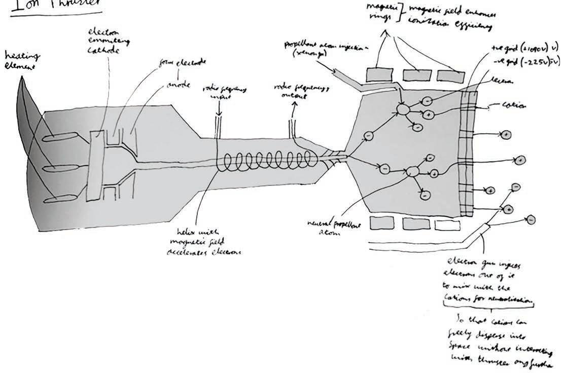
The first part of this system is an electron gun. A cathode is heated to make it emit electrons (through process of thermionic emission). Electrodes then generate an electric field to focus electron beams. To make sure the electrons travel the intended way, a large voltage between anode and cathode accelerates the electrons away from the cathode. They are then further accelerated by a radio frequency induced helix.

The second part of this system is a chamber that has been injected into with propellant atoms (usually xenon gas). The chamber is encased by magnetic rings which creates a magnetic field, which in turn enhances ionization efficiency. Electrons are then fired at the xenon atoms causing the atom to split into another electron and a cation. The electrons then stay in the chamber to ionize other xenon atoms, while the cation is accelerated out of a 2-sheet grid. One of these grids has a high positive voltage and the other has a high negative voltage. This creates a high potential difference accelerating the cations away from the spacecraft. m1u1 = m2v2 and so for each cation that is ejected, the spacecraft is given a force in the direction of its travel. Though cations weigh very little relative to the spacecraft, the sheer number ejected produces a high enough thrust to accelerate the spacecraft.

The spacecraft Dawn was able to reach 0.000115% speed of light using 425kg of xenon which amounts to an extortionate cost of $1,275,000. For this reason, more research is being done into alternative propellants, namely solid iodine which decreases not only cost but also storage volume. 425kg of iodine for example, would cost only $26,000.

Ionic propulsion requires a very high energy to accelerate propellant in return for very little thrust. This is fine for missions where the spacecraft can gradually be accelerated, as the thrusters can fire for years on end, however for missions closer to Earth, this is very inefficient compared to traditional methods of spaceflight such as fuel ejection. Furthermore, the little thrust means that drag and gravity cannot be overcome using this system and so alternate methods must be used to get the system into space.

Furthermore, the energy required must be obtained from somewhere. Currently solar panels do this; however, they produce very little power (usually 120kw depending on the time of day for example the space station which orbits Earth), especially for their size. Solar panels have only been proved successful up to the orbit of Jupiter with the success of the Rosetta space probe which had large 64sqm solar panels. So, what does the future of space flight look

like if we go down this path? Nuclear powered ionic propulsion systems. NASA came up with a design for this system which would dramatically increase the amount of electricity avaliable to be used hence accelerating each cation at a higher velocity. Unfortunately, this Jupiter icy moons orbiter mission powered by a nuclear electric xenon ion engine was cancelled in 2005 partly due to the quality of materials avaliable at the time. Since the first ion engine was developed by NASA in 1960 , the sheer scale of advancements is undeniable. New materials are being developed every day, so I think that in the next few years, nuclear-powered ionic propulsion systems such as the NEXI will be revisited.

Diagram of a nuclear-powered ion propulsion engine

“ Since the first ion engine was developed by NASA in 1960, the sheer scale of advancements is undeniable.

NUCLEAR PROPULSION

Having now talked about how nuclear power can be used in accompaniment with ionic propulsion, and how solar panels are not the future of space travel (especially travel in deep space), I will talk about a technology that will undisputably be up and coming in the next few decades. While there are several methods of using nuclear power to propel rockets, I will focus on two – namely nuclear electric propulsion, and more significantly in my opinion, nuclear thermal propulsion. Nuclear electric propulsion is where thermal energy is generated from the reactor, and then converted into electricity which is used to power an ion propulsion system.

This doesn’t use the nuclear power directly, raising the question of the efficiency of this system. Nuclear thermal propulsion skips the transfer of thermal energy to electricity. This method of propulsion provides high thrust: twice the propellant efficiency of traditional chemical rockets. This is important as it means flight crew can complete their missions faster and in turn are exposed to less cosmic radiation. The system works by transferring heat produced in a nuclear reactor to a liquid propellant which changes state to a gas, expanding through a nozzle and in turn propelling the spacecraft. One of the problems with this method of propulsion is that the materials inside the fission reactor must be able to withstand temperatures in the order of above 2700 degrees celcius. Traditional rockets are

developed using titanium and aluminium, however titanium has a lower melting point than 2700 at a mere 1725 degrees celcius. This means that, like the ionic propulsion system, the speed of material development is slowing down space progression. Science writer Jon Kelvey agrees that temperature is an issue and sees that the degradation of engine components will be caused by the extreme heat that is required. He also claims that “Today, there’s no nuclear fuel that can operate at that temperature for the desired period of time”.

Another issue with nuclear reactors with respect to space flight is ionizing radiation can permeate the reactor core leading to structural effects that may damage the reactor. This can be prevented with lead that can block this radiation; however, this adds weight to the craft slowing it down and hence making it more expensive to build and run.

While these systems are relatively safe once launched, nuclear thermal rockets are not suitable for launch from ground, as some of the exhaust emissions are radioactive and so a failed launch would be disastrous (radioactively messy and hard to clean up). This can be combatted by lab tests of the

engine which will reduce the chance of something going wrong. Like many of the issues, time is needed to solve them. This is why we don’t currently use nuclear thermal rockets and similarly why we will use them in the relatively near future.

As I have already alluded to in my introduction, it is important not to ignore the reason we are developing these technologies. While space exploration is obviously extremely important for reasons I have already covered, this nuclear method of propulsion is also applicable to systems we use on Earth. Most notably in marine travel where nuclear-powered submarines are already in use. The USS Nautilus was the first operational nuclear-powered submarine and was in commission for 26 years. Since she was able to stay under for far longer than diesel powered versions, she broke many records in her time. While we still have a long way to go to harness the true power of nuclear reactors, the reasons that I believe these devices are the future could span a whole essay of its own. The most notable advantages are that no greenhouse gases are produced, it is cost competitive with other fuels, reliable and most significantly devices do not need to be refuelled before every trip.

CONCLUSION

I have spoken about the traditional and arguably outdated liquid rocket engine, the challenges behind it such as fast fuel consumption with low rocket firing times, and a look into the future of these types of rockets. However, I am briefly concluding that liquid engines are not the future. A more current technology is the ionic propulsion system, which doesn’t have the issue of fast fuel consumption, allowing it to fire for years at a time. I then concluded by writing about what I believe the future of spaceflight looks like; nuclear powered systems. Whether that be nuclear powered ionic engines, or more futuristic nuclear thermal propulsion engines, I believe that these sorts of technologies are the future. This belief is backed up by NASA, where Bill Nelson introduced a project to design and demonstrate a working nuclear thermal rocket by 2027 to “expand the possibilities for future human spaceflight missions”. More broadly, NASA believes that these systems will be a “major investment in getting to Mars”. Nuclear powered systems being the future can also be seen on systems we use closer to home such as submarines and aircraft carriers. This therefore not only attests to the future being nuclear powered systems, but further backs up what I said in my introduction about the reasons we are even looking at space flight in the first place; our quality of life is improved with the advancement of spaceflight.

“ No greenhouse gases are produced, it is cost competitive with other fuels, reliable and most significantly devices do not need to be refuelled before every trip.

REFERENCES

1. Wendy Whitman Cobb. 2019. The Conversation. [Online] [Accessed 20 06 24]

2. Avaliable at: https://theconversation.com/howspacex-lowered-costs-and-reduced-barriers-tospace-112586#:~:text=For%20a%20SpaceX%20Falcon%20 9,is%20just%20%242%2C720%20per%20kilogram

3. Dawn (spacecraft). Wikipedia. [Online] [Accessed 20 06 24] Avaliable at: https://en.wikipedia.org/wiki/Dawn_(spacecraft)

4. Dawn: ion propulsion. NASA. [Online] [Accessed 20 06 24]

5. Avaliable at: https://science.nasa.gov/mission/ dawn/technology/ion-propulsion/

6. Professor Ondrej Muránsky. 2024. Ansto. [Online] [Accessed 20 06 24] Avaliable at: https://www.ansto.gov.au/our-science/ nuclear-technologies/reactor-systems/nuclear-propulsion-systems

7. World Nuclear Association. 2023. [Online] [Accessed 20 06 24] https://world-nuclear.org/information-library/economic-aspects/economics-of-nuclear-power#:~:text=Nuclear%20power%20plants%20 are%20expensive,a%20means%20of%20electricity%20generation.

8. H.G Kosmahl. 1982. A search for slow heavy magnetic monopoles. NASA. Available at: https://ntrs.nasa.gov/api/citations/19830002052/ downloads/19830002052.pdf [Accessed 26 June 2024].

9. Encyclopaedia Britannica, 2023. Electron gun. Available at: https://www.britannica.com/technology/ electron-gun [Accessed 26 June 2024].

10. Francis Davies. 2016. Advanced electric propulsion for next-generation space science missions. NASA. Available at: https://ntrs.nasa.gov/api/citations/20160014034/ downloads/20160014034.pdf [Accessed 26 June 2024].

11. European Space Agency, 2023. Frequently asked questions. Available at: https://www.esa.int/Science_Exploration/Space_Science/ Rosetta/Frequently_asked_questions [Accessed 26 June 2024].

12. Calomino, A., 2023. Space nuclear propulsion for human Mars exploration. NASA. Available at: https://www.nasa. gov/wp-content/uploads/2023/07/calomino-nuclear-v5. pdf?emrc=70cdca [Accessed 26 June 2024].

13. NASA, 2023. Space nuclear propulsion. Available at: https://www. nasa.gov/tdm/space-nuclear-propulsion/#:~:text=Nuclear%20 thermal%20propulsion%20provides%20high,thrust%20and%20 propel%20a%20spacecraft [Accessed 26 June 2024].

14. Steven Ashley, 2023. Ring of fire: Rocket engines put a new spin on spaceflight. Scientific American. Available at: https:// www.scientificamerican.com/article/ring-of-fire-rocketengines-put-a-new-spin-on-spaceflight/#:~:text=Rotating%20 detonation%20engines%20(RDEs)%2C,faster%20and%20 with%20larger%20payloads [Accessed 26 June 2024].

15. Navaz, Homayun K, Dix, Jeff C.1998. Evaluation of the Double-Hull Space Shuttle Tank Concept. NASA. Available at: https://ntrs. nasa.gov/citations/19990010036 [Accessed 26 June 2024].

16. NASA, 2021. Liquid rocket thrust. Available at: https://www.grc.nasa. gov/www/k-12/airplane/lrockth.html [Accessed 26 June 2024].

“ I believe the future of spaceflight looks like; nuclear powered systems.

HOW WILL OUR USE OF BIOMASS HELP US ADDRESS CLIMATE CHANGE?

STEM WILLIAM O'BRIEN

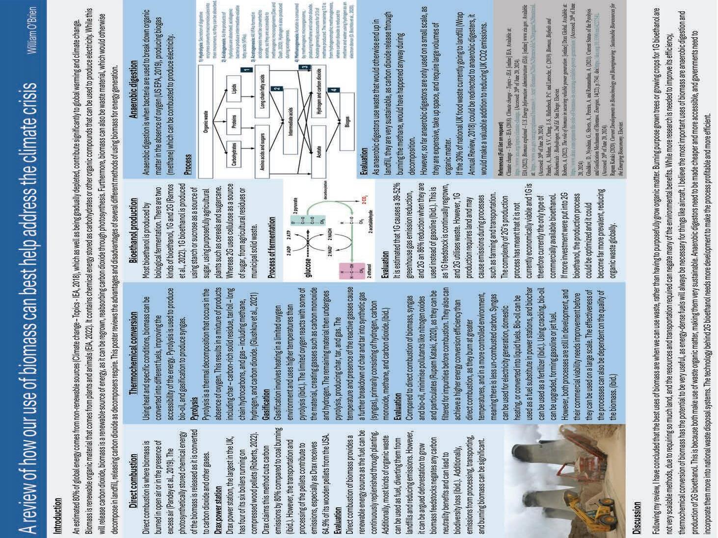
This

Independent Learning Assignment (ILA) was short-listed for the ILA/ ORIS Presentation Evening

INTRODUCTION

Roughly 80% of global energy comes from non-renewable sources,(Climate change – Topics - IEA, 2018) which as well as being gradually depleted, contribute significantly to global warming and climate change. This is because fossil fuels are stores of carbon, and combusting them means the release of carbon dioxide, a greenhouse gas. It is estimated that between 2030 and 2050, climate change will cause approximately 250,000 extra deaths per year.(WHO, 2023) Due to this, 196 countries pledged to limit

temperature increase to below 1.5 degrees Celsius above pre-industrial levels. This makes climate change a topic of global significance, and countries are forced to innovate new technologies to achieve this goal. Biomass is renewable organic material that comes from plants and animals.(EIA, 2022) It contains chemical energy stored as carbohydrates or other organic compounds, formed due to photosynthesis utilizing the sun’s energy. Biomass could be from purposely grown plants, or waste organic material.

The chemical energy in biomass can be converted into electricity in a similar way to fossil fuels. It is combusted to produce high-pressure steam, which turns a turbine attached to a generator. While this process does release carbon dioxide, biomass is a renewable and environmentally friendly source of energy. This is because its fuel can be regrown, reabsorbing carbon dioxide through photosynthesis. Furthermore, biomass can also be waste material, which would otherwise decompose in landfill, releasing carbon dioxide as decomposers respire. There are several different ways biomass can be treated or converted before combustion, each with its advantages and disadvantages. I am going to discus, direct combustion, thermochemical conversion, anaerobic digestion, and bioethanol production. (Bioenergy Technologies Office, n.d)

DIRECT COMBUSTION

Direct combustion is where biomass is burned in open air or in the presence of excess air.(Pandey et al., 2019) The photosynthetically stored chemical energy of the biomass is released as it is converted to carbon dioxide and other gases. This tends to take place in a furnace at 800-1000 degrees Celsius and works with any biomass with a low (<50%) water content.(Ibid)

Drax power station

Drax power station, the largest in the UK, has four of its six boilers running on compressed wood pellets. (Roberts, 2022) Drax claims these units generate 11% of the UK's renewable power, producing around 14 terawatt-hours annually.(ibid) They state this method cuts carbon emissions by 80% compared to coal burning.(ibid.)

However, it can be argued that the negative environmental impacts associated with deforestation counteract the environmental gain from not using fossil fuels. The transportation and processing of the pellets also contribute to emissions. Drax receives 64.9% of its wooden pellets from the USA. While Drax maintains its sources are sustainable, the long-term impact of large-scale biomass burning is still being evaluated.

Evaluation

Direct combustion of biomass provides a renewable energy source as the fuel can be continuously replenished through planting. Furthermore, unlike other renewable sources, biomass is not weather dependent and power plants can be turned on and off to meet energy demands (Mcfarland, 2017). Additionally, most kinds of organic waste can be used as fuel, diverting them from landfills and reducing emissions. However, it can be argued deforestation to grow biomass feedstocks negates any carbon neutrality benefits and can lead to biodiversity loss.(ibid) Additionally, emissions from processing, transporting, and burning biomass can be significant.

THERMOCHEMICAL CONVERSION

Using heat and specific conditions, biomass can be converted into different fuels, improving the accessibility of the energy. Pyrolysis is used to produce bio-oil, and gasification to produce syngas. Both substances are significantly more energy-dense than typical biomass and therefore can be more practical in many situations. For example, bio-oil from pyrolysis has the potential to be used as a sustainable aviation fuel.(Chuck, 2016)

Pyrolysis

Pyrolysis is a thermal decomposition that occurs in the absence of oxygen. The biomass is heated to a temperature of 400-700°C, causing complex molecules to break down into smaller ones. This results in a mixture of products including char - carbon-rich solid residue, tar/oil - long chain hydrocarbons, and gas - including methane, hydrogen, and carbon dioxide.(Glushkov et al., 2021)

Gasification

Gasification involves heating in a limited oxygen environment and uses higher temperatures than pyrolysis (>700°C).(ibid) The limited oxygen reacts with some of the material, creating gasses such as carbon monoxide and hydrogen. The remaining material then undergoes pyrolysis, producing char, tar, and gas. The temperature and presence of the reactive gasses cause a further breakdown of char and tar into synthetic gas,(syngas) primarily consisting of hydrogen, carbon monoxide, methane, and carbon dioxide.(ibid)

Evaluation

Compared to direct combustion of biomass, both syngas and bio-oil result in reduced emissions, minimising pollutants like nitrogen oxides and particulates,(Rupam Kataki, 2020) as they can be filtered for impurities before combustion. They also can achieve a higher energy conversion efficiency than direct combustion, as they burn at greater temperatures, and in a more controlled environment, meaning there is less un-combusted carbon. Syngas can be used for electricity generation, domestic heating, or converted into liquid fuels. Bio-oil can be used as a fuel substitute in power stations, and biochar can be used as a fertilizer.(ibid) Using cracking, bio-oil can be upgraded, forming gasoline or jet fuel due to shorter chain hydrocarbons. Aircrafts require high-energy-density sources of energy to limit weight and batteries are currently too heavy. This creates a market opportunity for a sustainable aviation fuel which biofuel could fill.

However, both processes are still in development, and their commercial viability needs improvement before they can be used on a large scale. The effectiveness of the processes can also be dependent on the quality of the biomass.(ibid)

ANAEROBIC DIGESTION

Anaerobic digestion is when bacteria are used to break down organic matter in the absence of oxygen. (US EPA, 2019) This results in the production of biogas (methane) which can be combusted to produce electricity. The process of anaerobic digestion has four successive stages; hydrolysis, acidogenesis, acetogenesis, and methanogenesis.(Meegoda et al., 2018)

1. Hydrolysis: Most macromolecules are too large to be directly absorbed by microbes, (Lutz-Arend Meyer-Reil, 1991) so must be broken into smaller components. This is done through the extracellular secretion of digestive enzymes from hydrolytic bacteria, converting carbohydrates, lipids, and proteins into sugars, fatty acids, and amino acids respectively.(Meegoda et al., 2018) These substances can diffuse through the cell membranes of the microbes.

2. Acidogenesis: As the products of hydrolysis are absorbed, acidogenic bacteria produce intermediate volatile fatty acids (VFAs).(ibid) VFAs are a class of organic acids, including acetates and larger organic acids like propionate and butyrate.

3. Acetogenesis: All VFAs formed in acidogenesis must be converted to acetate.(ibid) This is so they are accessible to methanogenic microorganisms, a type of archaea bacteria that produce methane as a metabolic by-product. (Das and Dash, 2020) Hydrogen is also produced during acetogenesis.

4. Methanogenesis: Acetate is consumed by methanogenic microorganisms, producing methane and carbon dioxide. Acetate generally accounts for 2/3 of methane produced. (Meegoda et al., 2018) The remaining third is from hydrogenotrophic methanogenesis, where carbon dioxide is reduced to methane and water using hydrogen as an electron donor.

(D. Bochtis et al., 2020)

Evaluation

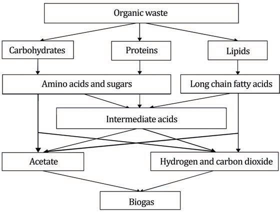
As anaerobic digestors use waste that would otherwise end up in landfill, they are very sustainable and arguably have no carbon footprint. Though burning the methane produced would release carbon dioxide, this would have happened anyway due to respiring bacteria as the biomass decomposes in landfill.

Anaerobic digestion has already proven to be very effective, 9% of UK farms disposing of waste this way. (GOV.UK, n.d) Many farmers digest slurry (manure and water), producing methane for energy, and then use the digestate as fertiliser. Nitrogen in digestate is more accessible to plants than it is in slurry making it a better fertiliser, and it also contains fewer pathogens so there is less risk to plants and animals.

(AFBI, 2016)

However, so far anaerobic digestors are only used on a small scale. As they are expensive, take up space, and require large volumes of organic matter, they are only financially viable for large farms.

As of 2018, 30% of UK food waste goes to landfill, and 41% is burnt or land spread.(Wrap Annual Review, 2018)

Use of anaerobic digesters for this volume of food would massively reduce emissions and produce large amounts of biogas.

BIOETHANOL PRODUCTION

Bioethanol is currently one of the most relevant biologically produced commodities. Most bioethanol is produced by biological fermentation, where the anaerobic respiration of organisms like yeast produces ethanol as they ferment organic matter. There are two kinds of bioethanol, 1G and 2G.(Ramos et al., 2022) 1G bioethanol is produced using starch or sucrose as a source of sugar, using purposefully agricultural plants such as cereals and sugarcane. Whereas 2G uses cellulose as a source of sugar, from agricultural residues or municipal solid waste.

(Gujer and Zehnder, 1983)

5.1. Process of Fermentation

The process of fermentation involves two stages, and overall converts glucose (from carbohydrate sources) into 2 ethanol molecules and 2 carbon dioxide molecules.

C6H12O6 → 2 C2H5OH + 2 CO2

The first stage is glycolysis, where glucose is converted into two pyruvate molecules.

C6H12O6 + 2 ADP + 2 Pi + 2 NAD+ → 2 CH3COCOO + 2 ATP + 2 NADH + 2 H2O + 2 H+

Pyruvate is a carboxylic acid (pyruvic acid). NAD is an electron carrier, and accepts electrons, being reduced to NADH. The ATP produced can be used by the cell to carry out cellular processes such as protein synthesis.

The second stage is pyruvate to ethanol conversion. Firstly, the carboxyl group of pyruvate is removed and released in the form of CO2, producing acetaldehyde. This is catalysed by pyruvate decarboxylase.

CH3COCOO + H+ → CH3CHO + CO2

The acetaldehyde molecule is then reduced by NADH, forming ethanol. This process also regenerates the NAD molecule from glycolysis. This reaction is catalysed by alcohol dehydrogenase.

CH3CHO + NADH + H+ → C2H5OH + NAD+ 1G or 2G Bioethanol

As opposed to 1G, 2G uses waste organic matter that would otherwise have no value, and would contribute to CO₂ emissions during decomposition if it was put in landfill. Solid waste management is estimated to contribute to around 5% of global emissions, and 61% of this waste is organic.(Choudhari, n.d) Utilising this waste would repurpose these emissions into energy production, greatly reducing the volume of fossil fuels burned. Furthermore, for 1G bioethanol production with corn grains, one-third of the grains are converted into ethanol, while the other two-thirds are converted into carbon dioxide and solid residues.(Iram, Cekmecelioglu and Demirci, 2022) Other

parts of the corn plant are also wasted, presenting a sustainability issue. With 2G, the feedstock is not limited to edible parts of plants, and waste or by product material can be used.

However, 2G requires more a complex pretreatment process. The feedstock for 2G bioethanol production are lignocellulosic materials, making the carbohydrates harder to access than starch in grains or sucrose in sugar cane. The enzymatic hydrolysis process also causes difficulty in 2G production, as expensive enzymes are required to break down the polymers involved. The long starch chains in 1G can be broken down by amylases and glucoamylases, while the lignocellulosic compounds in 2G require cellulases and hemicelluloses for hydrolysis.(Choudhari, n.d) The cost of these two processes has meant the current cost of 1G ethanol is 43% less than 2G.(Iram, Cekmecelioglu and Demirci, 2022)

Evaluation

The production of bioethanol has huge environmental benefits when compared to fossil fuels. It is estimated that 1G causes a 39-52% greenhouse gas emission reduction, and 2G an 86% reduction when they are used instead of gasoline. (Ibid) This is as 1G feedstock is continually regrown, and 2G utilises waste. However, the issues associated with their production processes limits their potential for wider use. 1G production requires land, involves waste, and may cause emissions during processes such as farming and transportation. The complexity of 2G’s production process has meant that it is not currently economically viable and 1G is therefore currently the only type of commercially available bioethanol.

If more investment were put into 2G bioethanol, the production process could be optimised and it could become far more prevalent, reducing organic waste globally. Both processes could also be combined and could complement each other.

Ethanol is an advantageous fuel source as it is biodegradable, can also be produced locally, and releases less pollutants than gasoline when combusted. It can be retrofitted into petrol engines with no modification required. Many countries already use bioethanol in combination with gasoline, with Brazil requiring a minimum of 27% ethanol in its fuel. (Transportpolicy.net, n.d) However, ethanol is less energy-dense than gasoline, reducing the fuel efficiency of cars. Furthermore, the transition to electric cars potentially makes investment in bioethanol redundant.

DISCUSSION

Originally, I believed direct combustion of biomass and 1G bioethanol production would be the best uses of biomass, as they are already quite prevalent. On researching, I realised other methods have far more potential, though are limited due to their early stage of development. In my opinion, the best uses of biomass are when we can use waste, rather than having to purposefully grow organic matter. Direct burning of biomass is profitable in some cases such as Drax, but that is with subsidies from the government. Burning purpose grown trees is not very scalable, due to requiring so much land, and waste must have a low enough moisture content to be usable. 1G bioethanol also requires land to grow its fuel, and its production process involves waste.

possible of the resources we extract. In order to scale these technologies, anaerobic digestors need to be made cheaper and more accessible, and governments need to incorporate them more into national waste disposal systems. The technology behind 2G bioethanol needs more development to make the process profitable and more efficient. While the shift to electric cars may remove a function of bioethanol, it also has the potential to be used for aviation fuel, boat fuel, and domestic heating.

SOURCE ANALYSIS

During my research, I used a total of 25 sources, involving 13 websites, 6 academic books, and 6 peer-reviewed journals. The validity of the books and journals can generally be trusted as they mostly consist of objective information which has been critically assessed and recognised through citing in other articles. However, there is always the potential for new or existing research to contradict some of the ideas I have used.

“ In my opinion, the most important uses of biomass are anaerobic digestion and production of 2G bioethanol.

12 of the 25 sources were written or last updated in the last 5 years, and an additional 6 in the last 10 years. While these are all relatively new sources, this is a constantly evolving subject, meaning some of the information used could be outdated. Furthermore, 3 sources were from 20 years or longer ago, and 4 were undated, which reducing their validity.

I believe that thermochemical conversion of biomass has the potential to be very useful, as energy-dense fuels will always be necessary for things like aircraft. However, the processes require lots of energy, so require more research to improve their efficiency. In my opinion, the most important uses of biomass are anaerobic digestion and production of 2G bioethanol. This is because both make use of waste organic matter, making them very sustainable. As the earth’s population is increasing, it is becoming increasingly important to make as efficient use as

Of the 13 websites used, 4 were official government organisation, and an additional 5 were government linked or officially recognised organisations. These sources can be trusted as they are well maintained by government departments, though there is still a small potential for bias in some contexts. 2 websites have unknown validity and therefore cannot necessarily be trusted. A further two were from companies, who could potentially profit more if certain ideas are promoted, meaning there is a potential of bias in the information given.

BIBLIOGRAPHY

1. AFBI (2016). 1 - Benefits of Anaerobic Digestion. [online] Agri-Food and Biosciences Institute. Available at: https:// www.afbini.gov.uk/articles/1-benefits-anaerobicdigestion. (Accessed: 20th of June 20, 2024).

2. Transportpolicy.net, (n.d.). Brazil: Fuels: Biofuels | Transport Policy [online] Available at: https://www.transportpolicy.net/standard/brazil-fuels-biofuels/#:~:text=Brazil. (Accessed: 20th of June 20, 2024).

3. BIOENERGY TECHNOLOGIES OFFICE (n.d.). Biopower Basics [online] Energy.gov. Available at: https://www.energy.gov/ eere/bioenergy/biopower- basics#:~:text=Biomass%20is%20 burned%20in%20a. (Accessed: 20th of June 20, 2024).

4. Chemistry (IUPAC), T.I.U. of P. and A. (n.d.). IUPAC - biotechnology (B00666). [online] goldbook.iupac.org. Available at: https://goldbook. iupac.org/terms/view/B00666. (Accessed: 20th of June 20, 2024).

5. Choudhari, A. (n.d.). Overview: Second Generation Bioethanol Process Technology. [online] Available at: https://www.tce. co.in/pdf/Overview- Second%20Generation%20Bioethanol%20 Process%20Technology.pdf. (Accessed: 20th of June 20, 2024).

6. Chuck, C. (2016). Biofuels for Aviation. Academic Press.

7. Climate change – Topics - IEA (2018). Climate change – Topics - IEA. [online] IEA. Available at: https://www.iea.org/topics/ climate-change. (Accessed: 20th of June 20, 2024).

8. Das, S. and Dash, H.R. (2020). Microbial and natural macromolecules: synthesis and applications. Amsterdam: Academic Press

9. Bochtis, D., Achillas, C., Banias, G. and Lampridi, M. (2020). Bio-economy and Agri- production. Academic Press.

10. EIA (2022). Biomass explained - U.S. Energy Information Administration (EIA). [online] www.eia. gov. Available at: https://www.eia.gov/energyexplained/ biomass/#:~:text=Biomass%20is%20renewable%20org anic%20material. (Accessed: 20th of June 20, 2024).

11. Glushkov, D., Nyashina, G., Shvets, A., Pereira, A. and Ramanathan, A. (2021). Current Status of the Pyrolysis and Gasification Mechanism of Biomass. Energies, 14(22), p.7541. doi: https://doi. org/10.3390/en14227541. (Accessed: 20th of June 20, 2024).

12. GOV.UK. (2023). Anaerobic digestion. [online] Available at: https:// www.gov.uk/government/statistics/farm-practices-survey-february2023-greenhouse- gas-mitigation/anaerobic-digestion#:~:text=In%20 2019%2C%20just%205%25%20of. (Accessed: 20th of June 20, 2024).

13. Gujer, W. and Zehnder, A.J.B. (1983). Conversion Processes in Anaerobic Digestion. Water Science and Technology, 15(8-9), pp.127–167. doi: https://doi.org/10.2166/ wst.1983.0164. (Accessed: 20th of June 20, 2024).

14. Iram, A., Cekmecelioglu, D. and Demirci, A. (2022). Integrating 1G with 2G Bioethanol Production by Using Distillers’ Dried Grains with Solubles (DDGS) as the Feedstock for Lignocellulolytic Enzyme Production. Fermentation, 8(12), p.705.

15. doi: https://doi.org/10.3390/fermentation8120705 (Accessed: 20th of June 20, 2024).

16. Lutz-Arend Meyer-Reil (1991). Ecological Aspects of Enzymatic Activity in Marine Sediments. Brock/Springer series in contemporary bioscience, pp.84–95. doi:https://doi.org/10.1007/9781-4612-3090-8_5. (Accessed: 20th of June 20, 2024)

17. Mcfarland, K. (2017). Biomass Advantages and Disadvantages. [online] SynTech Bioenergy. Available at: https://www. syntechbioenergy.com/blog/biomass-advantagesdisadvantages. (Accessed: 20th of June 20, 2024).

18. Meegoda, J., Li, B., Patel, K. and Wang, L. (2018). A Review of the Processes, Parameters, and Optimization of Anaerobic Digestion. International Journal of Environmental Research and Public Health, 15(10), p.2224. doi:https://doi.org/10.3390/ ijerph15102224. (Accessed: 20th of June 20, 2024).

19. Ostrem, K.M., Millrath, K. and Themelis, N.J. (2004). Combining Anaerobic Digestion and Waste-to-Energy. 12th Annual North American Waste-to-Energy Conference. doi: https://doi. org/10.1115/nawtec12-2231. (Accessed: 20th of June 20, 2024).

20. Pandey, A., Mohan, S.V., Chang, J.-S., Hallenbeck, P.C. and Larroche, C. (2019). Biomass, Biofuels and Biochemicals : Biohydrogen, 2nd Ed. San Diego: Elsevier.

21. Ramos, J.L., Pakuts, B., Godoy, P., García-Franco, A. and Duque, E. (2022). Addressing the energy crisis: using microbes to make biofuels. Microbial Biotechnology, 15(4), pp.1026– 1030. doi:https://doi. org/10.1111/1751-7915.14050. (Accessed: 20th of June 20, 2024).

22. Roberts, A. (2022). The role of biomass in securing reliable power generation. [online] Drax Global. Available at: https:// www.drax.com/opinion/the-role-of-biomass-in-securingreliable- power-generation/ (Accessed: 20th of June 20, 2024).

23. Rupam Kataki (2020). Current Developments in Biotechnology and Bioengineering : Sustainable Bioresources for the Emerging Bioeconomy. Elsevier.

24. US EPA (2019). How does anaerobic digestion work? [online] US EPA. Available at: https://www.epa.gov/agstar/how-doesanaerobic-digestion- work#:~:text=Anaerobic%20digestion%20 is%20a%20process. (Accessed: 20th of June 20, 2024).

25. World Health Organization (2023). Climate Change. [online] www. who.int. Available at: https://www.who.int/news-room/fact-sheets/ detail/climate-change-and- health#:~:text=Research%20shows%20 that%203.6%20billion. (Accessed: 20th of June 20, 2024).

26. Wrap Annual Review. (2018). Available at: https://www.wrap. ngo/sites/default/files/2020- 09/WRAP-Annual-Review-April2018-March-2019.pdf (Accessed: 20th of June 20, 2024).

AIRCRAFT CONTROL SYSTEMS

STEM SHREYAS

PASARKAR

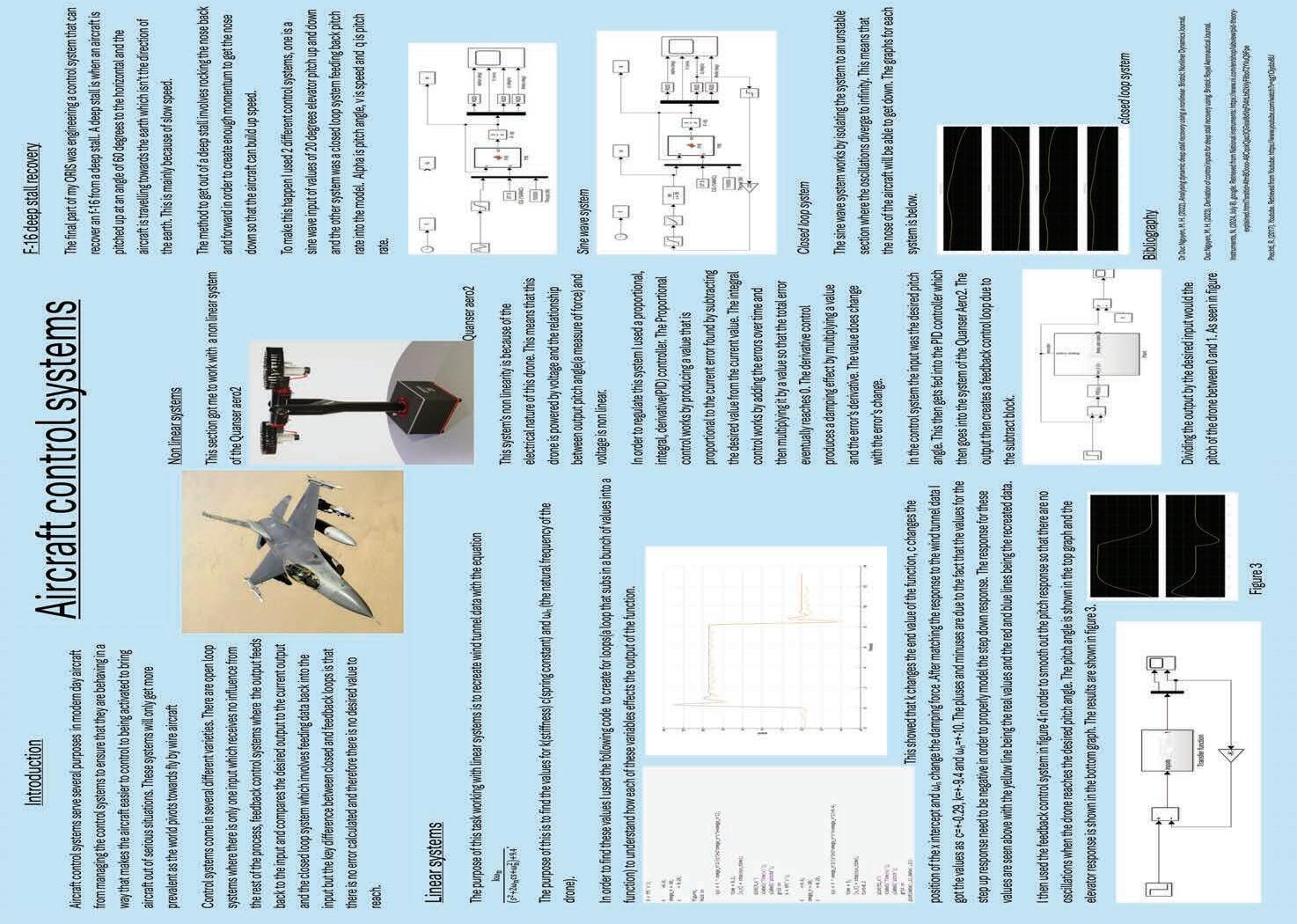
This Original Research in Science (ORIS) project was short-listed for the ILA/ ORIS Presentation Evening.

INTRODUCTION

Aircraft control systems serve several purposes in modern day aircraft from managing the control systems to ensure that they are behaving in a way that makes the aircraft easier to control to being activated to bring aircraft out of serious situations. These systems will most likely as time goes become more and more important with fly by wire being the main way in aircraft operate today. For example, one of the most famous examples of such systems is the MCAS system designed on the 737 Max variants. This control system works by auto trimming the aircraft down in order to stop the aircraft to over rotate at low speeds with flaps up which is especially common on take off.

Control systems come in several different varieties. There is the open loop system where there is only

one input which receives no influence from the rest of the process. This control system has its uses but it is also useless in several cases especially the pitch damping as that requires the input to be influenced by the output. To solve this problem there is a feedback control loop which is used extensively during this ORIS. The premise is that the output feeds back to the input and compares the desired output to the current output. This is used to determine the next steps to reach the output. The mechanisms behind this system is explored later. The final type of control system I use is a closed loop system. This also involves feeding data back into the input but the key difference between closed and feedback loops is that there is no error calculated and therefore there is no desired value to reach.

METHOD AND EXPLANATION OF RESULTS

Linear System

The recreation of the wind tunnel data allowed me to find certain values for constants that dictate the behaviour of the aircraft seen in the transfer function . A transfer function is a function that is used to simulate the behaviour of a system in terms of inputs and outputs. Using code in MATLAB that simulated the step response from 0 to 10 degrees in elevator pitch I found the values for k, c and ωn¬ where c is damping force k is stiffness And ωn is natural frequency Initially I created for loops (figures: 2, 3 and 4) in order to see how these variables effected the output of the transfer function and the results are below for the step up.

Figure 1 to 4 (top left to bottom right):

Figure 2: For loop for c between 0.1 and 0.8 Figure 3: For loop for k between 5 and 10, Figure 4: For loop for ωn between 5 and 15

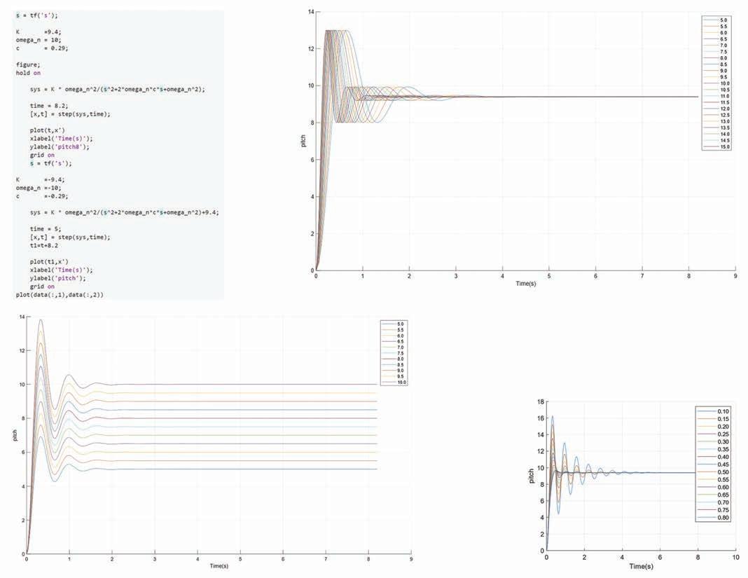
After matching the values in the for loops to what recreated the original data I found that c=+-0.29, k=+-9.4 and ωn=+-10. The pluses and minuses are due to the fact that the values for the step up response need to be negative in order to properly model the step down response. The graph produced is figure 5 with the blue and red lines being the step up and step down responses while the yellow line is the original data. The data was designed to be the original data but transposed up do that the start and end pitches are 0.

5

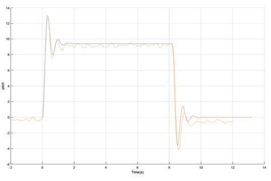
“ A transfer function is a function that is used to simulate the behaviour of a system in terms of inputs and outputs.

The numbers were then put into the transfer function in the control loop in figure 6 with a slight change as k is really 10 times a constant and that therefore means that in actuality k was 0.94. The point of the feedback control is to decrease the pitch rate closer to the ending pitch. The control loop is seen in figure 6. This effectively creates an auto-trim system.

Figure

Figure 6

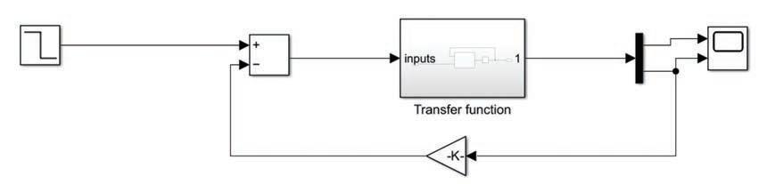
The input in this case is a step down response of the desired elevator pitch from 10 to 0 degrees which gives the step up and down response as the initial step up is also completed before the step down. This then enters the transfer function which then gets fed into the demux block which shows both pitch in the top input and then differentiates this to get pitch rate as the bottom output. This is then fed through a gain which acts as a constant that gets multiplied to the pitch rate which then gets fed back into a subtract block. The difference between the desired outcome and the current pitch rate is the calculated and fed back into the loop again till the elevator reaches 10 or 0 degrees. The results of this loop is seen in figure 7. The top graph is the pitch angle and bottom graph is pitch rate on the y axis and time on the x axis.

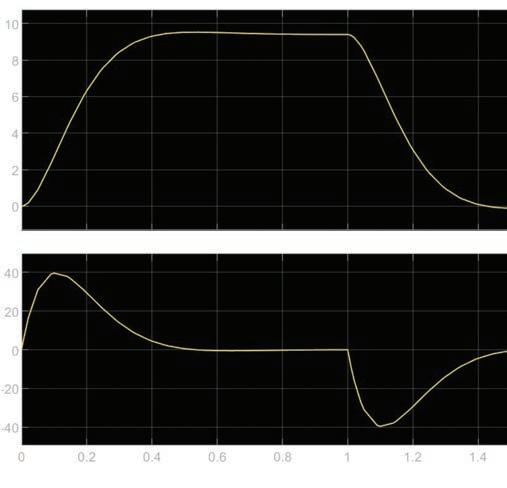
The non linear system involved the use of the Quanser Aero2 which I a drone /helicopter generally used in universities.

The nature of it being non linear is due to the fact that this is an electronic drone and therefore it is supplied with voltage and the relationship between voltage input and output in terms of pitch angle is non linear and a distinct curve is seen as in figure 8. figure 8 is a graph of voltage against pitch angle.

Quanser Aero2

Figure 7

Non Linear System

Figure 8

I then created a control system for this using a PID or proportional, integral, derivative controller. The Proportional control works by producing a value that is proportional to the current error found by subtracting the desired value from the current value. The integral control works by adding the errors over time and then multiplying it by a value so that the total error eventually reaches 0. The derivative control produces a damping effect by multiplying a value and the error’s derivative. The value does change with the error’s change. (National_Instruments, 2024)

In the control system the input was the desired pitch angle. This then gets fed into the PID controller which then goes into the system of the Quanser Aero2. The output then creates a feedback control loop due to the subtract block. The control system can be seen in figure 9.

Figure 9

In order to see the differences between the responses I plotted a graph of theta against theta f which makes the final value that the simulation converges to is 1. This means that it is much easier to compare the different outputs as they all converge to the same number. This is achieved by dividing the output by what the desired output should be. The results are shown in figure 10. There is a 20 degree line but it is below the 30 degree line. This creates another simple auto trim system.

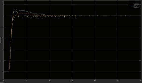
10

Figure

F-16

This was the final part was to bring an F-16 out of a deeps stall. A deep stall is a phenomenon where an aircraft is in a pitch up attitude of in the simulation’s case around 60 degrees, but instead of flying towards the direction that the nose is pointing the aircraft is instead travelling at an angle at something like 50 degrees below the horizon. A large part of this phenomenon is the fact that the aircraft is flying at speeds much lower than its stall speed. A deep stall looks something like figure 11.

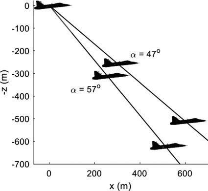
In this case the aircraft has a nose up of 57 and 47 degrees and the black line shows the actual path of flight.

This phenomenon is caused by the disruption of air by the wing passing through the area where the elevators are. The wing wake then renders the elevators almost useless as there is no longer a slipstream for the elevator to manipulate.

The method to recover deep stall comes from a paper written by Duc Nguyen et al (Duc Nguyen, 2023) and it works by oscillating the stick in a sin wave pattern for 1.25 cycles before then going full nose down. The oscillations will build up enough momentum to get the nose down which is important as this allows the aircraft to build up speed and get out of the deep stall. The control system, seen in figure 12, is made by simply inputting a sin wave into the F-16 model.

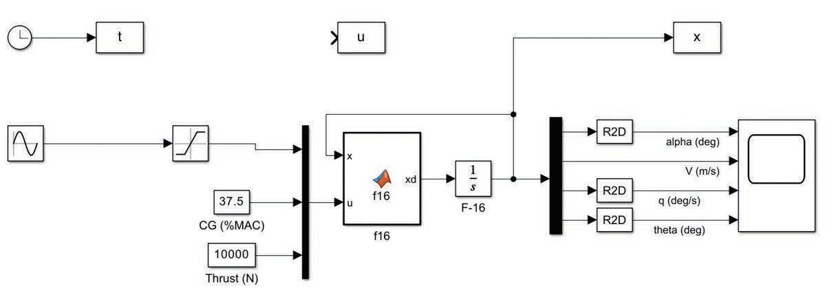
The values used for the sin wave are amplitude of 20 and the frequency is 1 rad/s. The amplitude in this case corresponds to the pitch angle of the elevators. The choice of these numbers is to try to get a solution in an unstable area. Using figure 13 the red area is the unstable region and I red off the graph to determine the frequency. The reason why the method targets the unstable region is because the oscillation amplitude diverges to infinity. This means that it is possible to get the nose down to a pitch of anywhere below 0 degrees. This facilitates deep stall recovery.

Figure 11 (Dr Duc Nguyen, 2022)

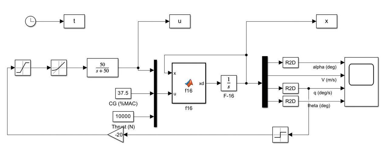
This method of recovery from deep stalls has been found empirically by pilots but it often involves the pilot observing the oscillation of the aircraft. An example of this is this video at time 6:20 .(Prechtl, 2017) However, to do this manually gets even harder when the workload of the pilots during a deep stall this method is not 100% foolproof and could result in pilots reacting too late and therefore not being able to recover from the deep stall. Further explanations of the physics behind this method of recovery can be seen in the papers by Dr Duc Nguyen in the references.

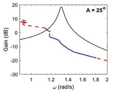
I also created another method to bring an F-16 out of a deep stall which is to create a closed loop system that feeds back pitch rate into the F-16. This causes the nose to drop just like the previous method and it takes around 2 seconds faster to get the nose to 0 degrees compared to the previous system. The results and control systems are seen in figure 14 and 15.

“ It is possible to get the nose down to a pitch of anywhere below 0 degrees. This facilitates deep stall recovery.

Figure 13 (Dr Duc Nguyen, 2022)

Figure 14

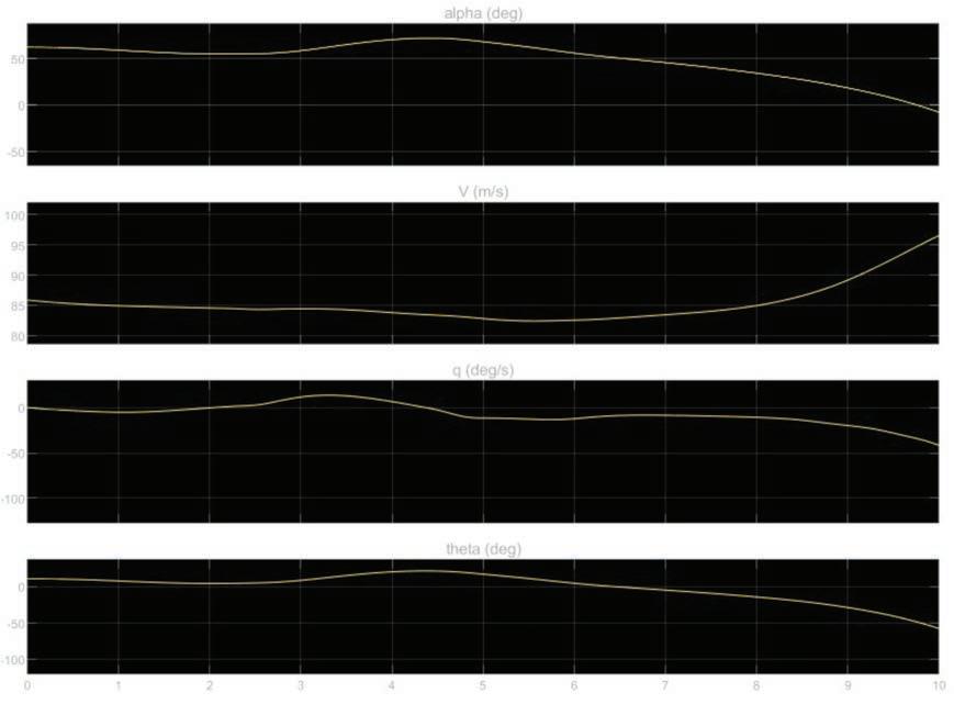
The control system in figure 15 works by taking the current sign of whatever the pitch angle, multiply the number by -20 and then feeding back into the F-16. There are some extra blocks added in there to make it more realistic. For example there is a rate limiter that limits the rate of movement of the stabiliser to maximum 60 degrees a second as this method is often a lot more aggressive in terms of elevator movements as seen in figure 16. This means that rather the elevator pattern being a square wave pattern there are periods where the elevator pitch is smoothed out. There is then a transfer function that further improves the realism. Both systems have in common a block that limits the maximum value and minimum value of the elevators and the T block in the top left just counts the time and this allows me to make the videos.

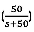
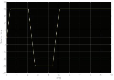
Again with this simulation all the pilot needs to do in this case is just manage the system as a few moments after this simulation the pitch angle has an infinite gradient going downwards.

Figure 15

Figure 16

CONCLUSION, EVALUATION AND POTENTIAL FURTHER RESEARCH

Linear

Overall the recreation of data and the control system did work and it provided a much more oscillation free pitch up and down. The possible next step would be to introduce a white noise function that can generate noise as seen in the original data. This will help to make the simulation more realistic and the system can therefore be fine tuned to further improve the response given. Furthermore a rate limiter could also be added to ensure that the elevator is travelling within it’s achievable bounds.

Non linear

The creation of the non linear system was successful as I did manage to get results that are what should be expected for this system. A potential next step for this is to introduce noise or realistic model the air currents and see how this model holds up. The basis for working with non linear systems also greatly helped me when it came to working with he F-16 as the paper where the method of deep stall recovery came from used non linear analysis.

F-16

The oscillation model to recover from a deep stall worked very well and provided a working method to get out of a deep stall. There were a few issues like understanding the scientific paper to work out what values to use for the frequency a but those issues were cleared up.

Further research in this specific system of deep stall recovery could be to further current research on T tailed aircraft as they are more susceptible to deep stalls due to the position of their elevators. The closed loop system also successfully recovered an F-16 out of a deep stall. However, this method of deep stall recovery could most likely only work with fighter jets such as the F-16 because their elevators are made up fully by their horizontal stabilisers. This means that the F-16 gets greater ability to pitch its nose down compared to a T tailed aircraft due to the larger area of the elevators. This means that there is a high chance that this recovery system will not work for any T tailed aircraft or simply any aircraft whose elevators consist of small tabs on the horizontal stabiliser.

BIBLIOGRAPHY

1. Dr Duc Nguyen, M. H. (2022). Analysing dynamic deep stall recovery using a nonlinear. Bristol: Nonliner Dynamics Journal

2. Duc Nguyen, M. H. (2023). Derivation of control inputs for deep stall recovery using. Bristol: Royal Aeronautical Journal

3. Instruments, N. (2024, July 8). google. Retrieved from National instruments: https://www.ni.com/en/shop/ labview/pid-theory-explained.html?srsltid=AfmBOoooA9CqokQjaz3QGsiaI8dVqF04ItLb62kVyF8boT2YVuQ9Fpe

4. Prechtl, R. (2017). Youtube. Retrieved from Youtube: https://www.youtube.com/watch?v=qg1Ojydzv8U

ACKNOWLEDGEMENTS

I would like to thank Dr Duc Nguyen at the aeronautical engineering department at Bristol University for not only allowing me to do this research project with him but also for teaching me how to use 2 new programmes, MATLAB and Simulink and get me well up to speed enough to be able to work on and complete the above research

GLOSSARY AND NOMENCLATURE

1. Nose: The front end of the aircraft that is just further forward than the pilot.

2. Angle of attack: This is the angle that the wing makes the oncoming air. This can be further extrapolated to the nose’s angle to the oncoming air.

3. For loop: A loop where the code runs the same process but for a range of values. The start and end values as well as the difference between each term can be specified in MATLAB using special notation.

4. Step up and step down: A sudden change of value from a base value, most of the time 0, to another value either higher or lower for example 10.

5. Control system: A system that regulates the behaviour of in this research project’s case an aircraft.

6. Stall speed: The stall speed is the lowest possible speed that an aircraft can sustain flight.

7. T tailed aircraft: Aircraft whose horizontal stabilisers rest on the vertical stabiliser. This results a formation that looks like a T. Examples of this can be seen with many small sized airliners and especially private jets such as any jet that is manufactured by Gulfstream.

8. Auto trim: A system that manages the pitch of the aircraft so that it keeps the aircraft flying at the same attitude(pitch relative to horizon) by moving the elevators slightly.

9. Nomenclature.

10. Angle of attack is denoted as α

11. Direction of travel of the aircraft is denoted as γ

12. Time is denoted as t

13. Velocity is denoted as v

14. Pitch angle is denoted as ϑ.

INITIATING THE

DEVELOPMENT OF A LIBRARY FOR PLASTIC POLYMERS USING RAMAN SPECTROSCOPY

JOEL SELLERS

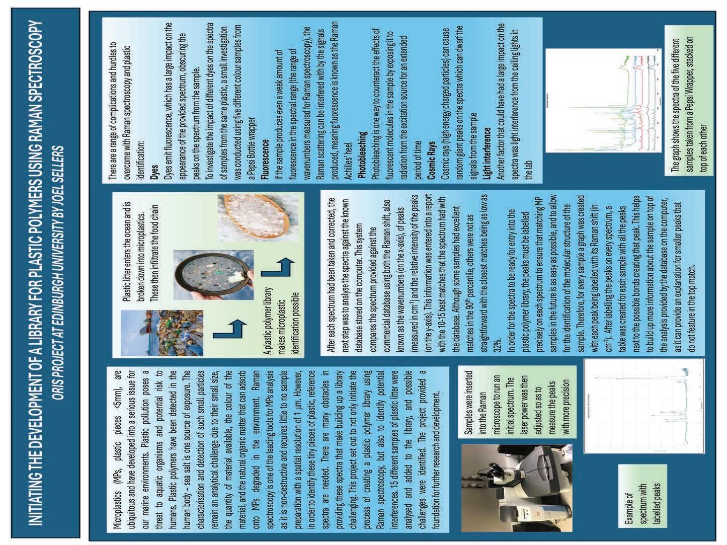
This Original Research in Science (ORIS) project won the 2025 ORIS award.

INTRODUCTION

Plastic, due to its versatility and functionality, is used in a range of different circumstances including many single-use items such as packaging. A poor recycling system for plastic polymers has resulted in plastic accumulating in the environment.1 Despite most plastic waste going into landfill where it remains for many hundreds of years due to its long decomposition time, 2 some waste ends up in the aquatic environment, with an estimate in 2019 saying that around 171 trillion plastic particles,

primarily microplastics (MPs, plastic particles <5mm in size), are floating in the sea.3 MPs can be categorised into two sources: primary MPs, which are particles manufactured to be a microscopic size, and secondary MPs, which form from the breakdown of larger pieces of plastic on land and at sea through weathering.4 The buildup of these MPs in aquatic environments has a negative impact as it is a direct threat to the marine food chain.19 It not only decreases the life span of organisms impacted

(usually through eating MPs or by eating smaller organisms that have) but also poses a human risk as the levels of toxicity might build up through the trophic levels.5

Detecting and characterising MPs in environmental samples represents an analytical challenge. MPs are problematic to analyse mainly due to their small size (<5mm), and there are intrinsic difficulties in collecting, handling, identifying and characterising MPs from environmental samples.6 The two most popular analytical tools used for identifying these MPs at the moment are Raman spectroscopy and FT-IR (Fourier Transform - Infra-Red) spectroscopy.7 In this instance, there is an advantage for using Raman spectroscopy as Raman has a spatial resolution of 1µm which is much better for MP analysis than the 100µm spatial resolution of FT-IR. The measurements of both FT-IR and Raman are complementary as Raman spectroscopy allows better identification of non-polar, symmetric bonds whereas FT-IR gives clearer signals of polar groups.16 Raman spectroscopy is ideal for MP analysis as it is generally non-destructive and requires little to no preparation of the sample.18 Due to its small spatial resolution of 1 µm it has the capacity to analyse a wide range of MP sizes, i.e above 1 µm.20 Raman spectroscopy is an increasingly popular analytical tool used for a range of disciplines from chemistry8 to medicine9 to geology.10

Raman spectroscopy works by measuring the shift in frequency of inelastically scattered light which it creates by firing photons at the sample using an excitation source, i.e a laser. Scattered

light is made up of two parts: elastic scattering and inelastic scattering. Elastic scattering has the same wavelength and frequency as the photons from the laser and is much more common whereas inelastic scattering, which only happens to one out of every 107 photons,11 changes frequency which is then measured in order to work out the molecular structure of the sample. This scattered light is produced by a photon from the laser hitting a molecule of the sample which emits a scattered photon. If the scattered photon has a lower frequency than the photon from the laser then this is called Stokes Raman scattering and if it has a higher frequency, it is named anti-Stokes Raman scattering.11 Different shifts are characteristic of certain functional groups, allowing us to piece together the structure of the molecule from its Raman 'fingerprint' (see figure 1 for an example).

Figure 1: Shows the Raman spectrum of polystyrene. We can reconstruct the shape of the molecule by looking at the Raman shift of the peaks, so, for example, the large peak at ~ 1150 cm -1 corresponds to a C-C stretch and the peak at ~ 1450cm -1 corresponds to CH 2 scissoring (a certain type of bending vibration of CH 2 groups)

METHOD

Sample Collection

Initially 15 samples were collected from commonplace plastic items (mainly food packaging). These samples were prepared by cutting them into small pieces varying in size from 1cm to 3cm using scissors. The aim was to provide at least three pieces per sample where possible, as there was a risk of samples being burned by the laser during Raman spectroscopy if due care was not taken. These samples were sorted into 15 labelled plastic pots and handled using tweezers to minimise interference with the spectra that might have been caused by human touch. The samples were placed onto a glass microscopic slide, with non-flat samples being weighed down on both sides by smaller glass slides.

Interference investigation

In order to investigate the effects of different dyes on the same plastic, five samples were cut from the wrapper on the outside of a Pepsi bottle (see table below), one for each of the five colours used in the wrapper. Despite all coming from the same wrapper, there were many differences between the spectra which will be described in depth later (see 7. Pepsi Wrapper comparison).

The tables contain the names of all 15 samples, with a photograph of the samples next to a ruler, and finally the parameters used when producing their Raman spectrum.

The work was completed using the Raman microscope (see figure 2). The prepared slide was inserted into the instrument onto the bed, which was further moved using the joystick so that the sample was directly under the beam of light. Then the doors were shut, and the microscope was focused using the wheels under the bed to get it close and the wheel on the side of the joystick was used to adjust it. A picture was taken of the sample under the microscope in order to compare any visible similarities at a later date.

Initial steps of optimisation

The first step once the sample was ready was to run a quick test to produce rough initial spectra. Turning off the lights in the lab was essential in order to reduce the level of interference with the spectra caused by exterior photons entering the instrument (see 6.5 Light Interference). Running the initial spectrum was useful to enable changes to the laser power in real time, allowing us to see whether the sample will produce a weak or strong spectrum, and also to test what laser power the sample can withstand for an extended period of time. The camera showing the microscope’s image of the sample shut off when the laser was on so the next step was to check that the sample had not been burned by the laser, although this did not happen at all. If the sample

showed strong peaks when using 1mW excitation (laser power), the laser power was turned down to 0.5mW to see whether the peaks were just as strong, as having a high excitation, whilst increasing the strength of the peak, also lowers the wavenumbers of the peaks, allowing them to bunch up more and become less distinct.

Exposure time

The exposure time was the time taken to run one spectrum and increasing exposure time increases the strength of the peaks. Generally, 60 seconds exposure time was used, however for some samples with very strong results, 45 seconds or even 30 seconds exposure time were sufficient.

Spectra

The final parameter modified was the number of times spectra were taken, with the minimum for the instrument being two as it takes an average between the two, eliminating false peaks that originate from cosmic rays and other interference (see section 6. Issues with identification). Mostly five spectra were taken per sample with a few exceptions for which only three spectra were obtained. The laser wavelength of the instrument used was 785nm.

Background correction

After the spectra had been taken and the final spectrum had been produced, a few issues needed to be dealt with in order to create the best spectrum for that sample. In order to counteract the interference caused by fluorescence, we added a fluorescence filter through the instrument’s software to the spectrum which removed the hump in the baseline (see figure 3). The fluorescence filter subtracts the background by taking advantage of the fact that the curvature of the baseline is much less sharp than that of the Raman peaks.

Almost all spectrum still needed some manual baseline correction as the baseline (see figure 3) was not level. A spline tool was used to select points along the actual baseline in order to give the final spectrum a straight baseline. This was essential when dealing with the data as clear spectra are needed when it comes to future use for MP identification.

Figure 2: The instrument used; a Thermo Scientific™ DXR3 Raman Microscope equipped with a 785nm excitation laser source

Figure 3: Graph A shows the spectrum of a sample taken from a Pepsi Bottle before baseline correction – the curved baseline shape is due to fluorescence. Graph B demonstrates the same spectrum but after using baseline correction techniques. The techniques used for this spectrum were applying a fluorescence filter and manually correcting the baseline using a spline tool (see above for details)

ANALYSIS OF RESULTS

After each spectrum had been taken and corrected, the next step was to analyse the spectra against the known database stored on the computer. This system compares the spectrum provided against the commercial database using both the Raman shift, also known as the wavenumbers (on the x-axis), of peaks (measured in cm-1) and the relative intensity of the peaks (on the y-axis). This information was entered into a report with the 10-15 best matches that the spectrum had with the database. Although some samples had excellent matches in the 90th percentile, others were not as straightforward with the closest matches being as low as 32%.

The reason these spectra have been taken is to initiate the creation of a Raman spectra library for plastic polymers. In order for the spectra to be ready for entry into the library, the peaks must be labelled precisely on each spectrum to ensure that matching MP samples in the future is as easy as possible, and to allow for the identification of the molecular structure of the sample. Therefore, for every sample a graph was created with each peak being labelled with its Raman shift (in cm-1) (see figure 4).

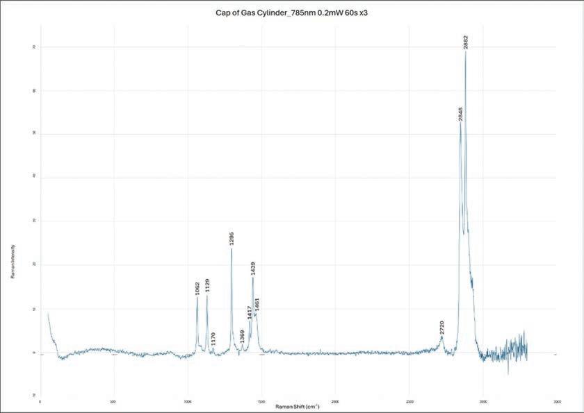
Figure 4: Example of spectrum with labelled peaks

After labelling the peaks on every spectrum, a table was created for each sample with all of the peaks next to the possible bonds creating that peak. This helps to build up more information about the sample on top of the analysis provided by the database on the computer, as it can provide an explanation for smaller peaks that do not feature in the top match. For all labelled peak tables see section.12 Data

ISSUES WITH IDENTIFICATION

There are a range of complications and hurdles to overcome with Raman spectroscopy and plastic identification.

Dyes

Dyes, along with other additives to plastic such as pigments, can have a significant effect on the ability to recognise the spectrum of the sample.12 This is because the dyes emit fluorescence, which has a large impact on the appearance of the provided spectrum, obscuring the peaks on the spectrum from the sample.

To investigate the impact of different dyes on the spectra of samples from the same plastic, a small investigation was conducted using five samples from a Pepsi Bottle wrapper – each one being a different colour (see figure 7: Pepsi Wrapper Comparison for results).

Fluorescence

Fluorescence is caused by the absorption of light by a molecule, which excites the molecule to a higher electronic state. The molecule drops back down to its ground energy state by vibrational relaxation and the emission of a photon with a lower energy than the initial photon, meaning it has a higher wavelength and a lower frequency. If the sample produces even a weak amount of fluorescence in the spectral range (the range of wavenumbers measured for Raman spectroscopy), the Raman scattering can be interfered by the signals produced, meaning fluorescence is known as the Raman Achilles’ heel 13 785nm is a near-IR (or NIR) wavelength that is a very popular excitation source for Raman spectroscopy as it minimises the effect of fluorescence whilst also providing strong Raman peaks.14 This is because the energy of the excitation source is not enough to excite the molecule to the higher electronic state.15

Photobleaching

Photobleaching is one way to counteract the effects of fluorescent molecules in the sample by exposing it to radiation from the excitation source for an extended period of time. Whilst we did not intentionally use this technique as a counter to fluorescence, as we were exposing the sample to the laser whilst running the test spectrum, the computer system warned us that the spectrum showed signs of photobleaching which would have probably minimised fluorescence (as none of the samples showed any sign of burning or extreme degradation after the test spectrum).

Cosmic Rays

Cosmic rays (high energy charged particles) can cause random giant peaks on the spectra which can dwarf the signals from the sample. These are easy to spot as they create very sharp peaks on the spectrum. They have no influence on the final spectrum provided as they disappear once the second exposure has ended and the anomaly has been taken out. This is due to cosmic rays random nature in time and space, meaning that as long as you run two exposures (which is the minimum anyway), you can easily overcome this obstacle.

Light Interference

Another factor that could have had a large impact on the spectra was light interference from the ceiling lights in the lab. Photons from the lights were finding their way into the instrument whilst the spectrum was being taken and creating false peaks which decreased our ability to match the spectrum in the future effectively.

In order to illustrate this, a spectrum was taken with the lights on and with no laser power, meaning that any peaks provided were from the lights, and a spectrum was then taken with the lights off and no laser power (see figure 5).

In order to counteract this effect, we conducted all of the tests with the lights off so as not to have any false peaks on our spectra which would cause later problems.

Figure 5: As is clearly visible, the light being switched on caused around seven peaks that would not have been created if the light had been off

PEPSI WRAPPER COMPARISON

The five spectra produced from the different colours of the Pepsi Wrapper were all unique, despite some showing a few similarities between each other. In order to demonstrate the differences between the spectra, all of the data was added to the same graph with five different lines on it (representing the five colours) and the lines were put one above each other in order for similarities and differences to be more clear (see figure 6).

Figure 6: Spectra of the five different samples taken from Pepsi wrapper, stacked for a clearer reading. Only the Raman shift (the x-axis) is relevant here as Raman intensity (y-axis) doesn’t help much with the compare of the peaks

Although this does show some similarities between the more prominent spectra, blue and green, it doesn’t allow for any comparison with the weaker signals such as white or black. In order to make the signals more equal, the y-axis was changed from Raman Intensity (which is very different between colours) to relative intensity (relative to the highest peak on the spectrum).

7: This graph shows the spectra of the five samples

However, this is very noisy due to the lower S/N (signal/noise) of the weaker spectra. In order to compare all of the lines, we looked at the tables produced for the five colours earlier in the analysis of results section (for table see Data section at the end). This made it easier to distinguish common and unique peaks for each spectrum.

Another interesting difference between the five colours were the large differences in Raman intensity (which can be observed in figure 6). Green gave the strongest signals with a highest intensity of around 125, with blue second with 81. The other three spectra were significantly less intense which could be explained in a few ways.

First of all, we are going to assume that the wrapper is made of one base plastic polymer which is then dyed in order to create the colours.

One possible explanation is that the red, black and white dyes were metal based, which could obscure/ dampen the strength of the signals from the plastic behind. Most metals and alloys are Raman inactive due to their electronic structures and symmetry.

The more probable explanation is that the dye/ colourant in the red, black and white samples produced fluorescence in the measured range which drowned out the signal from the plastic. It has been reported that the colour of plastic particles can influence the quality of the provided spectra, and that the measurements of red and yellow particles are usually more affected.17 Therefore the reason that the spectra were so weak, is because the peaks have been covered up by a much larger amount of fluorescence by comparison to the green and blue samples.

Figure

taken from a Pepsi wrapper after having changed the y-axis to relative intensity instead of Raman intensity

CONCLUSION

In conclusion, the time spent on this project has started the process of building a polymer library. The initial analysis has highlighted a number of issues that will continue to be a challenge as further plastics are added. However, these challenges need to be overcome in order to produce a comprehensive database that can be referred to in the future.

During the course of the project, 15 different plastics were analysed and added to the polymer library. Even with this limited sample size, there were significant challenges with fluorescence and dyes. This highlights the scale of the challenge associated with MP analysis. However, as this project is conducted on a larger scale, it is likely that more plastics with similar properties will be identified.

“ During the course of the project, 15 different plastics were analysed and added to the polymer library. Even with this limited sample size, there were significant challenges with fluorescence and dyes.

FURTHER POSSIBLE RESEARCH

The next steps for this research would be to take the 15 plastic samples and break them down into MP pieces using cryomilling. These MPs could then be examined in order to see any differences in the spectra provided or could be exposed to aquatic conditions and more degradation in order to simulate the effects of MPs within the marine environment for an extended period of time. After this it would be interesting to compare the results provided from Raman spectroscopy in order to understand the effect of these conditions on the molecular composition of the MPs, and to assess the difficulty in identifying these MPs compared to the large plastic litter.

ACKNOWLEDGEMENTS

I would like to thank Dr Maya Al-Sid-Cheikh for all of her help in not only facilitating the project but also for reading through and checking my report. She was extremely generous with her time throughout. I would also like to thank Andrei for patiently supervising me whilst producing the Raman spectra and for highlighting some key interferences with the results.

BIBLIOGRAPHY

1. Pinto, J. and Teresa A.P. Rocha-Santos (2017). Microplastics – Occurrence, Fate and Behaviour in the Environment. Comprehensive Analytical Chemistry, pp.1–24. doi: https://doi.org/10.1016/bs.coac.2016.10.004

2. Cole, M., Lindeque, P., Halsband, C. and Galloway, T.S. (2011). Microplastics as contaminants in the marine environment: A review. Marine Pollution Bulletin, [online] 62(12), pp.2588–2597. doi: https://doi.org/10.1016/j.marpolbul.2011.09.025

3. Eriksen, M., Cowger, W., Erdle, L.M., Coffin, S., Villarrubia-Gómez, P., Moore, C.J., Carpenter, E.J., Day, R.H., Thiel, M. and Wilcox, C. (2023). A growing plastic smog, now estimated to be over 170 trillion plastic particles afloat in the world’s oceans— Urgent solutions required. PLOS ONE, 18(3), p.e0281596. doi: https://doi.org/10.1371/journal.pone.0281596

4. Cole, M., Lindeque, P., Halsband, C. and Galloway, T.S. (2011). Microplastics as contaminants in the marine environment: A review. Marine Pollution Bulletin, [online] 62(12), pp.2588–2597. doi: https://doi.org/10.1016/j.marpolbul.2011.09.025

5. Margeta, A., Šabalja, Đ. and Đorđević, M. (2021). The presence and danger of microplastics in the oceans. Pomorstvo, 35(2), pp.224–230. doi: https://doi.org/10.31217/p.35.2.4

6. Pinto, J. and Teresa A.P. Rocha-Santos (2017). Microplastics – Occurrence, Fate and Behaviour in the Environment. Comprehensive Analytical Chemistry, pp.1–24. doi: https://doi.org/10.1016/bs.coac.2016.10.004

7. Käppler, A., Fischer, D., Oberbeckmann, S., Schernewski, G., Labrenz, M., Eichhorn, K.-J. and Voit, B. (2016). Analysis of environmental microplastics by vibrational microspectroscopy: FTIR, Raman or both? Analytical and Bioanalytical Chemistry, [online] 408(29), pp.8377–8391. doi: https://doi.org/10.1007/s00216-016-9956-3

8. Hess, C. (2021). New advances in using Raman spectroscopy for the characterization of catalysts and catalytic reactions. Chemical Society Reviews, [online] 50(5), pp.3519–3564. doi: https://doi.org/10.1039/D0CS01059F

9. Vlasov, A.V., Maliar, N.L., Bazhenov, S.V., Nikelshparg, E.I., Brazhe, N.A., Vlasova, A.D., Osipov, S.D., Sudarev, V.V., Ryzhykau, Y.L., Bogorodskiy, A.O., Zinovev, E.V., Rogachev, A.V., Manukhov, I.V., Borshchevskiy, V.I., Kuklin, A.I., Pokorný, J., Sosnovtseva, O., Maksimov, G.V. and Gordeliy, V.I. (2020). Raman Scattering: From Structural Biology to Medical Applications. Crystals, [online] 10(1), p.38. doi: https://doi.org/10.3390/cryst10010038

10. Fries, M. and Steele, A. (2018). Raman Spectroscopy and Confocal Raman Imaging in Mineralogy and Petrography. Springer series in surface sciences, pp.209–236. doi: https://doi.org/10.1007/978-3-319-75380-5_10

11. Jakob Thyr and Edvinsson, T. (2023). Evading the Illusions: Identification of False Peaks in Micro-Raman Spectroscopy and Guidelines for Scientific Best Practice. Angewandte Chemie International Edition, 62(43). doi: https://doi.org/10.1002/anie.202219047

12. Zhao, S., Danley, M., Ward, J.E., Li, D. and Mincer, T.J. (2017). An approach for extraction, characterization and quantitation of microplastic in natural marine snow using Raman microscopy. Analytical Methods, 9(9), pp.1470–1478. doi: https://doi.org/10.1039/c6ay02302a

13. Gérard Panczer, Dominique De Ligny, Mendoza, C., Gaft, M., Anne-Magali Seydoux-Guillaume and Wang, X. (2015). Raman and fluorescence. European Mineralogical Union eBooks, pp.61–82. doi: https://doi.org/10.1180/emu-notes.12.2

14. Granite (n.d.). Reducing Fluorescence in Raman Spectroscopy. [online] Edinburgh Instruments. Available at: https://www.edinst. com/how-to-reduce-fluorescence-in-raman-spectroscopy/

15. Cebeci-Maltaş, D., Alam, Md Anik, Wang, P. and Ben-Amotz, D. (2017). Photobleaching profile of Raman peaks and fluorescence background. European Pharmaceutical Review, [online] 22(6), pp.18–21. Available at: https://www.europeanpharmaceuticalreview. com/article/70503/raman-peaks-fluorescence-background/

16. Lenz, R., Enders, K., Stedmon, C.A., Mackenzie, D.M.A. and Nielsen, T.G. (2015). A critical assessment of visual identification of marine microplastic using Raman spectroscopy for analysis improvement. Marine Pollution Bulletin, [online] 100(1), pp.82–91. doi: https://doi.org/10.1016/j.marpolbul.2015.09.026

17. Nava, V., Frezzotti, M.L. and Leoni, B. (2021). Raman Spectroscopy for the Analysis of Microplastics in Aquatic Systems. Applied Spectroscopy, 75(11), pp.1341–1357. doi: https://doi.org/10.1177/00037028211043119

18. Frost, R., Kloprogge, T. and Schmidt, J., 1999. Non-destructive identification of minerals by Raman microscopy. Internet Journal of Vibrational Spectroscopy, 3, pp.1-13.

19. Yuan, Z., Nag, R. and Cummins, E. (2022). Human health concerns regarding microplastics in the aquatic environment - From marine to food systems. Science of The Total Environment, [online] 823(153730), p.153730. doi: https://doi.org/10.1016/j.scitotenv.2022.153730

20. Anger, P.M., von der Esch, E., Baumann, T., Elsner, M., Niessner, R. and Ivleva, N.P. (2018). Raman microspectroscopy as a tool for microplastic particle analysis. TrAC Trends in Analytical Chemistry, 109, pp.214–226. doi: https://doi.org/10.1016/j.trac.2018.10.010

HUMANITIES ARTS &

RUVIN MEDA WINNER OF ARTS AND HUMANITIES

WHY DEMOCRACY FAILED IN RUSSIA AFTER THE FALL OF THE SOVIET UNION ARTS HUMANITIES

GEORGE CHRISTIANSEN

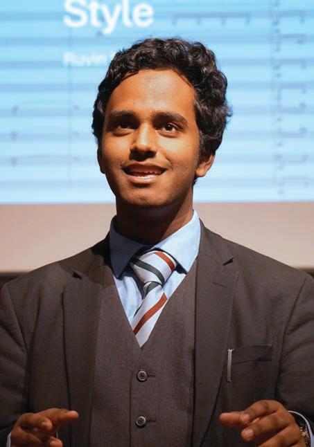
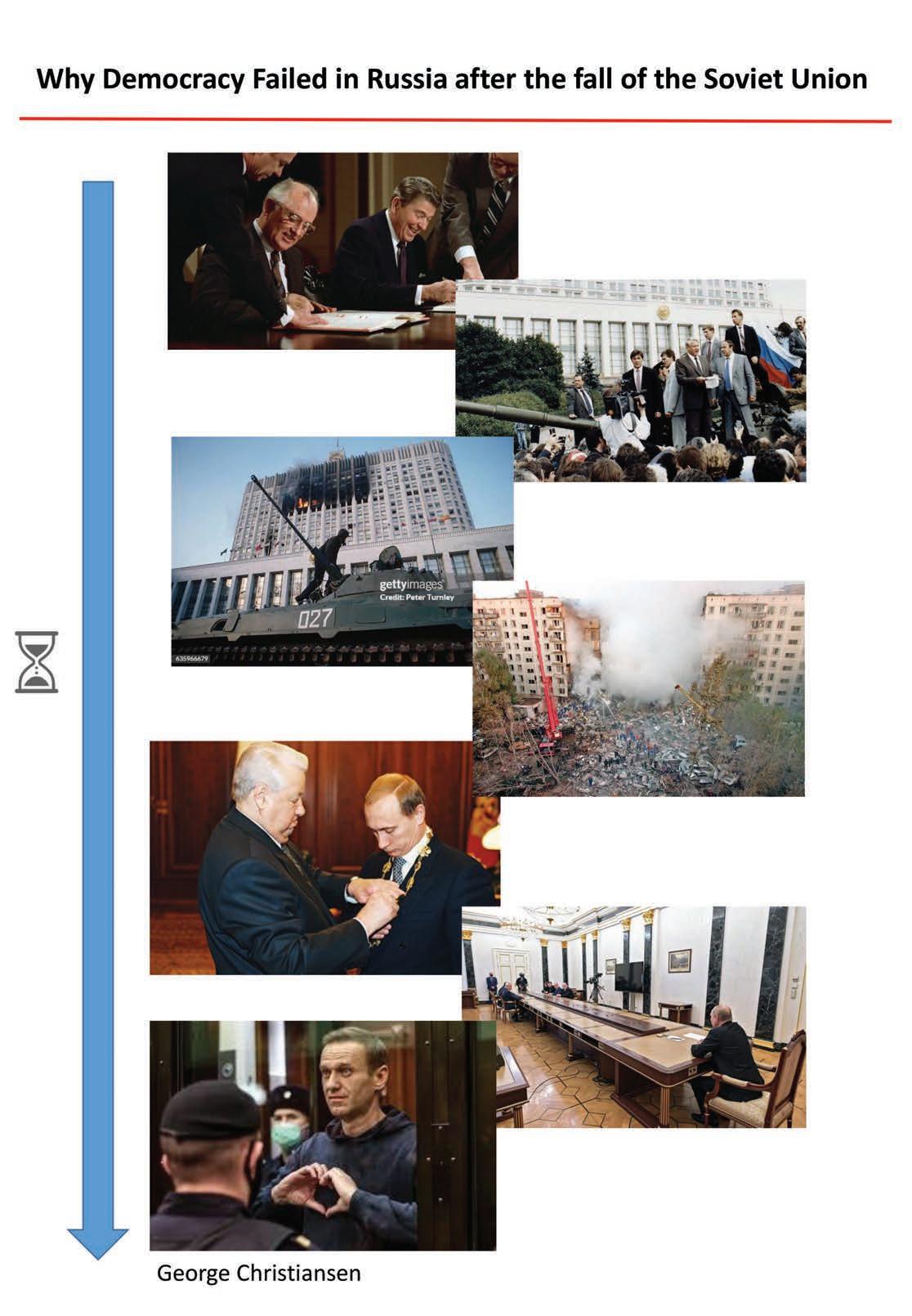
This Independent Learning Assignment (ILA) was short-listed for the ILA/ ORIS Presentation Evening.

Following the collapse of the Soviet Union in 1991 and the defeat of Communism, the western democratic system seemed invincible. This attitude was epitomised in the words of Fukuyama, that the failure of Communism marked “The universalisation of Western liberal democracy as the final form of human government”. (1989: 4) However, such optimism was mistaken. Russia, the central entity of the Soviet bloc and the most powerful post-communist state is a dictatorship; elections are rigged, freedom of speech and information is supressed and opposition to Putin’s regime is stifled. In the prescient words of Richard Nixon in 1992, “The Communists have been defeated, but the ideas of freedom are now on trial”.

That democracy failed its greatest trial in the modern era is indisputable. The focus of this essay is to explain why.

Russia’s vast natural resources and possession of the world’s largest nuclear arsenal ensures that its politics remain highly relevant to international affairs. As demonstrated by Putin’s invasions of Georgia and Ukraine, the consequences of Russian dictatorship are not just domestic; the failure of democracy has given to rise to one of the greatest threats to international security in the modern world. However, Putin’s regime cannot last forever and the opportunity for democracy in Russia will arise again.

Should democracy take root in Russia, it would set an example to autocracies and repressed peoples across the globe that they too can democratise. To increase its chances of future success, we must understand why Russian democracy failed before. The failure of democracy in Russia is often attributed to excessively rapid economic liberalisation. Some authors hold that Russia's autocratic history and culture is incompatible with democracy. These are not views that I share. I attribute the failure of democracy in Russia to four key factors. Firstly, the homogenisation of society under Soviet rule and the failure of Gorbachev’s perestroika reforms left Russia without a civil society, which impeded the growth of political parties and an organised democratic movement. Secondly, in the absence of a civil society to drive change from below, democratic reforms had to be directed from above, making the ruling elite’s commitment to democracy critical to its success. However, the vast majority of Russian elites, including President Yeltsin, were not democrats and the foundations of democracy were poorly laid. Thirdly, Yeltsin’s lawless transition from the Soviet command economy to a market economy plunged tens of millions into poverty whilst creating a small circle of elites with vast wealth and power, which stilted the rise of an independent and politically active middle class and left the population disillusioned with the turmoil of post-Soviet Russian democracy. Finally, the rise of Putin to the presidency and his destruction of Russia’s fledgling democratic institutions marked the

end of Russia’s transition from a failing democracy to a dictatorship.

The absence of an established civil society in Russia after the collapse of the Soviet Union, particularly of autonomous societal organisations, considerably hindered democratisation. Civil groups representing special interests, such as independent trade unions, charities and pressure groups, were entirely foreign to the Russian people, as unofficial organisations had been banned under Soviet rule. As a result, there were no significant independent civil organisations to represent and uphold the interests of the Russian people and to push for transparent, democratic government. By contrast, the Polish trade union movement, ‘Solidarity’, played a major role in the collapse of Communism in Poland, leading negotiations for the successful democratic transition and its leader, Lech Wałęsa, became the first democratically elected president of Poland. Russia also lacked strong popular support for democracy, which was seen in other post-communist countries where democratisation was successful. In November 1991, polls showed support for autocratic rule at 39%, which rose to 51% after one year of nominally democratic rule under Yeltsin.(Steele, 1994) This likely stemmed from a view of the Soviet Union not as a foreign, oppressive force, but as a state centred on Russia, so opposition to the USSR and its autocratic system of government was not as strong as in other post-communist states. Russia’s autocratic history and culture is not

however, incompatible with democracy, as some propose. Other post-communist countries with little previous experience of democracy or civil society, such as Romania, Bulgaria and Mongolia, have had successful democratic transitions and indeed almost every modern democracy has, whether gradually or suddenly, at some point adopted democracy for the first time. Moreover, the assertion that Russian culture is incompatible with democracy relies on the false assumption that culture cannot change. Rather, it is a perpetually changing phenomenon that can adapt to embrace democratic traditions. A communist and autocratic past may be an impediment to democracy, but cross-national comparison shows that it is not insurmountable. However, without broad public support, democracy cannot succeed. As a result of widespread apathy towards democracy, nascent democratic institutions in Russia were dismantled virtually unopposed, as there were few democratically elected liberals who were able to scrutinise Yeltsin’s reforms and hold Russian democracy to account. By contrast, successfully democratic post-communist countries had popular civic movements that pushed for democracy. For example, ‘Solidarity’ had 10 million members at its peak and in 1989, people in the Baltic States formed a 2 million strong human chain to oppose Soviet rule. The lack of a strong civil society in Russia minimised pressure on the elites to commit to real democratisation and facilitated the erosion of democratic institutions without opposition.

“ Popular political parties are central to democracy as they are the basis on which governments are formed and similar views and interests are politically organised.

Popular political parties are central to democracy as they are the basis on which governments are formed and similar views and interests are politically organised. As a result of 70 years of Communist rule, which had homogenised Russian society and supressed independent civil organisations, there were few groups with special interests to represent in the early 1990s, so it was difficult for political parties to differentiate themselves.(Fish, 2005) This was reinforced by Gorbachev’s decision to hold the 1990 parliamentary elections before legalising political parties, which set a precedent of personality politics and political individualism, alongside reducing the incentive for investment in parties. This prevented the rise of extensive political parties that could form governments and engage in meaningful debate. This is evidenced by the 25 officially registered parties by mid-1992 which had greatly overlapping policies. Membership of political parties was also very low, demonstrating public indifference towards party politics after 75 years of oppressive Communist Party rule and mandatory attendance at mass party rallies. For example, the largest party, the Democratic Party of Russia, had under 30,000 members in a country of 148 million.(Steele, 1994) This lack of engagement deprived parties of funds, preventing them from launching large-scale campaigns to gain widespread support. Although factions of those with similar ideologies were formed in Parliament in place of parties, these were very loose with no inner-factional discipline or instructions on how to vote. Initially,

the factions began to take root and were on track to become parties in all but name, but they were undermined by Yeltsin’s actions. Upon being elected President, Yeltsin resigned from ‘Democratic Russia’ and refused to co-operate with the factions. Given the power of the presidency in Russian politics and Yeltsin’s initially unrivalled popularity, his decision to ignore party politics undermined a key component of the democratic apparatus.(Steele, 1994) Without established political parties, organisation and legislation in the Russian Parliament was significantly impeded, undermining the democratic process of government.

Given the weakness of Russian civil society and party politics, democracy rested upon the commitment of the elites, particularly Yeltsin, to establish and respect democratic norms. However, despite his rhetoric, Yeltsin’s political decisions undermined the democratic institutions that relied on his support to succeed.(Hamburg, 1998) Yeltsin not only disregarded party politics, but largely ignored Parliament throughout his tenure. Presidential collaboration with a strong parliament is vital to ensure political discussion and compromise, a key feature of democracy. However, in his first year of rule, Yeltsin accepted from Parliament the right to rule by decree. Whilst this initially reflected his dedication to radical market reforms rather than his disregard for democracy, Yeltsin continued to rule by decree after his special powers had run

out, diminishing the authority of Parliament and subverting the rule of law. During the October 1993 Constitutional Crisis, Yeltsin was impeached following his unconstitutional dissolution of Parliament in September and calling of early elections, and Rutskoy, the vice-president, was proclaimed president. The Deputies in Parliament, including the Speaker and vice-president, barricaded themselves inside the parliament building. Having just two years earlier stood on a tank outside the White House and condemned the August Coup against Gorbachev by Communist hardliners, Yeltsin ordered tanks to bombard the building and hundreds of unarmed civilians were indiscriminately shot dead by the police. Rather than seek a democratic compromise, Yeltsin responded to a threat to his authority with aggression in a remarkably Soviet manner. This was not the limit of Yeltsin’s disregard for democracy. After the 1995 parliamentary elections in which the Communists won by far the most seats and their presidential candidate, Zyuganov, was beating him in the polls, Yeltsin drafted a decree to suspend the presidential election but was dissuaded from issuing it at the last minute. He also tampered with the 1996 presidential election, with his campaign manager conceding that “of course” the rules of campaigning were breached.(Satter, 2016) Yeltsin’s blatant disregard for the most fundamental institutions of democracy, the constitution and elections, indicates that he was not a committed democrat, but rather a populist opportunist, prepared to revert to autocratic practices to maintain his grip on power. Yeltsin not only sidelined Parliament through ruling by decree, but in 1993 he codified in the new Russian constitution a presidency with nigh-on dictatorial powers, rendering the legislature insignificant. The effective super-presidency created by Yeltsin made discourse and compromise unnecessary by sidelining Parliament, the forum for political discussion. In post-communist countries, there is a strong positive correlation between the strength of the legislature and the strength of democracy. Countries with strong parliamentary powers, such as Latvia and Czechia, had considerably more open politics by 2002, than countries with weak legislatures, such as Russia and

Kyrgyzstan.(Fish, 2005) Yeltsin’s creation of an almost dictatorial presidency combined with his disregard for the framework of democracy perpetuated autocratic traditions in post-communist Russia. In the words of Robert Service, “In the guise of the president, Yeltsin ruled like a General Secretary”. (2009, p. 513) His political decisions undermined Russian democracy before it could really take root.

It was not just Yeltsin, however, who was uncommitted to democracy; the Soviet-era nomenklatura continued to dominate politics, perpetuating the anti-democratic practices of the Soviet regime. The nomenklatura comprised 78% of regional elites in 1992 and dominated the upper echelons of politics.(Snegovaya, 2023) For example, Gerashchenko, the head of the Russian Central Bank from Summer 1992, had been the head of the Soviet Central Bank and Chernomyrdin, Yeltsin’s second prime minister from December 1992 to 1998, was a Communist Party veteran and had been the Soviet Minister of Gas Industry. Even Gaidar, Yeltsin’s first prime minister and a radical free market economist, had been a longstanding member of the Communist Party. There is a very strong correlation

in post-communist countries between high levels of elite rotation and a successful democratic transition. (Fish, 2005) For example, by 1993 in Poland and Estonia, former Communist Party members comprised just 30% and 40% of the political elite respectively, far below the levels in Russia.(Snegovaya, 2023) The persistence of Soviet-era elites and Yeltsin’s antidemocratic political decisions perpetuated autocratic traditions and prevented a clean break from dictatorial rule. The economic situation in Russia in the 1990s was arguably the most significant contributor to the failure of democracy. The greatest challenge facing Yeltsin and the leaders of post-communist Russia was to oversee a successful transition from the crumbling and hugely inefficient Soviet command economy to a market economy. Whilst other post-communist countries succeeded, Yeltsin failed in this challenge and the 1990s were a decade of economic catastrophe. The ensuing collapse in living standards was unparalleled in peacetime Russian history and exceeded that in Weimar Germany and the United States during the Great Depression This was the consequence of the timidity of Yeltsin’s economic reforms, the proliferation of corruption

and the collapse of the rule of law over which he presided. Yeltsin’s initial economic reforms were incontestably pro-market. He appointed the free-market economist Yegor Gaidar as his first prime minister, who was committed to ‘shock therapy’, the rapid liberalisation of Russia’s economy. Gaidar immediately removed price controls after taking office in January 1992, which caused inflation to soar to 245% in January alone.(Hamburg, 1998) Many, including the market economist Yavlinsky argued, “liberalising prices without privatising the economy and breaking the monopolies was a major mistake”. However, in the first half of 1992, monopolies were obliged to abide by pre-defined limits on profitability ratios, so this was likely not the cause. Regardless, soaring inflation wiped out savings and plunged millions into poverty, causing resentment towards the 'shock therapy' approach. In the face of increasing opposition to Gaidar’s reforms, Yeltsin backtracked. In July 1992, Yeltsin appointed Gerashchenko to be the head of the Russian Central Bank. Gerashchenko printed money and expanded the credit facilities of large companies, undermining Gaidar’s plan to reduce inflation.(Service, 2009) In 1995 he was labelled by Jeffrey Sachs, “the worst central banker in the world”. Gaidar’s other liberalising reforms of restructuring state spending and slashing cheap state credits to businesses encountered opposition from powerful factory directors. By mid-1992, Gaidar’s shock therapy had been abandoned. Plans to slash military spending were overturned and the government froze oil and gas prices.(Fish, 2005) In December, Yeltsin replaced Gaidar as prime minister with Chernomyrdin, a gradualist, officially ending 'shock therapy'. During 1992, industrial output collapsed by 18% and inflation, which had previously been non-existent, soared to 2500%. Under Chernomyrdin, the deregulation that was necessary for businesses to thrive in a liberal economy was neglected, massive state subsidies for the oil and gas industry were retained, ministers refrained from legislation on land privatisation and there were persistent restraints on entrepreneurial activity.

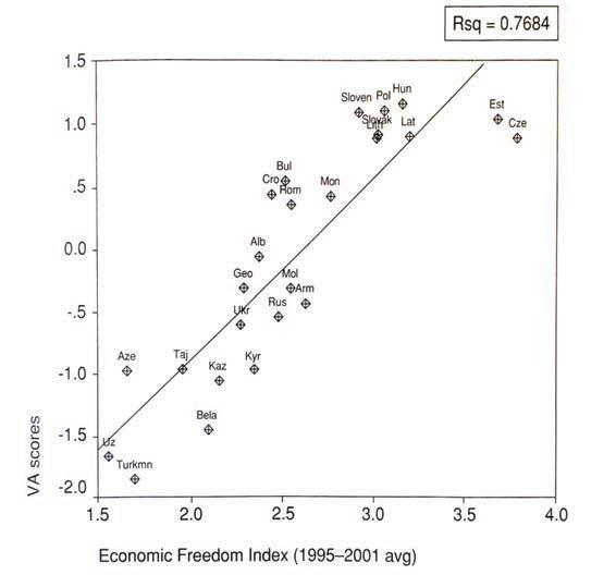
Correlation between VA scores, a measure of political openness, and economic freedom in the post-communist region (Fish, 2005, p. 149)

Throughout the 1990s, Russia ranked far below more democratic post-communist countries in the Economic Freedom Index. As shown in the graph above, there is a strong correlation in the post-communist region between economic and political freedom. Countries with the greatest economic liberalisation, such as Poland, Hungary and Slovenia, had the most successful democratic transitions. A key reason for this is that predatory overregulation in Russia and other undemocratic post-communist countries stifled entrepreneurship and retarded the growth of an independent middle class; by 2005, there were just six small businesses per 1000 people in Russia, compared with 30 per 1000 in Eastern-European countries such as Poland, that embraced rapid economic opening (Fish, 2005). An autonomous middle class plays a vital role in challenging the political establishment and supporting democracy. In the words of Moore, “No bourgeoise, no democracy”.

Yeltsin’s embrace of gradualism condemned the 1990s to be a decade of economic and social catastrophe. By 1995, life expectancy for men had collapsed to 57, and as shown in the graph below, between 1992 and 1998, GDP almost halved as industrial production plummeted by 56%; a greater decline than during WW2.(Service, 2009) The failure of Yeltsin’s economic reforms to create a flourishing market economy, due to the abandonment of shock therapy, caused widespread poverty and discontent with post-Soviet Russian democracy in Russia.

Yeltsin oversaw a collapse in the rule of law. By 1992, crime had increased by 70% from 1989, and the murder rate tripled to 40,000 annually.(Satter, 2016) Contract killings of rival businessmen became commonplace, as criminal gangs were closely intertwined with the state and the rulings of the judiciary were for sale.

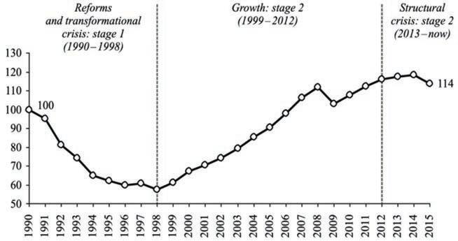
Changes in Russian GDP from 1990 to 2015 (Rosstat, 2016)

Yeltsin also oversaw a collapse in the rule of law and the institutionalisation of corruption, resulting in the creation of the oligarchy and a venal state that could not be truly democratic. The scale of corruption under Yeltsin’s rule was immense. The police and courts were utterly corrupt, generals sold equipment to the highest bidder including Chechen terrorists and cheap loans given to companies to pay workers’ wages were embezzled with the profits split between factory and bank managers, whilst workers went unpaid.(Service, 2009) Indeed, Yeltsin himself was implicated in a corruption scandal and, in 1999, he removed his newly appointed prime minister, Stepashin, for refusing to keep the anti-corruption investigators away from the Yeltsin family. The culture of unfettered criminality and corruption over which Yeltsin presided was not one in which capitalism and democracy could succeed. It was not just that corruption thrived in post-Communist Russia, but

The lawless transition to a market economy over which Yeltsin presided resulted in the creation of the oligarchy, and precipitated stark economic inequality which caused resentment against liberal democrats who were seen as responsible. The privatisation of state companies through the provision of vouchers to every adult citizen was unlike the process in any other post-communist country, and was rightly called "economically ineffective and politically illiterate" by the leader of the opposition. Vouchers were bought up by company managers and criminal gangs, creating ‘nomenklatura privatisation’ as two-thirds of privatised enterprises were acquired by incumbent managers. (Fish, 2005) The loans-for-shares scheme of 1995-96 sold 21 of the most valuable state enterprises in closed auctions for criminally low prices, far below their actual value. The venture netted a mere $700 million, a tiny proportion of the companies’ actual value, whilst creating a class of super-rich oligarchs to the detriment of the Russian people.(Satter, 2016) Overall, Gaidar’s shock therapy started Russia off on the road to a prosperous market economy; the initial recession and high inflation caused by his reforms was the unavoidable consequence of undoing 60 years of Stalinist planning. Yeltsin’s dilution of the reforms upon encountering significant resistance prevented the rise of a truly economically free and mobile populace, which would have greatly aided democracy. In the words of Constant,

“Commerce

inspires in men a vivid love of individual independence"

By the end of the 1990s, Yeltsin’s antidemocratic policies and lawless transition to a market economy had impeded democratic institutions and brought Russia’s nascent democracy to its knees. The appointment of Putin in August 1999 as vice-president and his rise to the presidency in 2000 was the final blow to a failing system. Putin openly showed his disdain for democracy, claiming the fall of the USSR was “The greatest geopolitical catastrophe of the 20th century”, and he set about dismantling Russia’s remaining democratic institutions. Under Putin’s regime, corruption has thrived, increasing tenfold between 2001 and 2005 to the point where spending on bribes was roughly equivalent to tax revenue at over $316 billion a year. (Satter, 2016) Freedom of the press has been eradicated and elections, including the 2000 presidential election, are rigged. Any public opposition is stifled, often through the state sponsored murder of high-profile political opponents such as Alexei Navalny and Boris Nemtsov, and investigative journalists like Anna Politkovskaya and Dmitri Bykov. Worse, in order to maintain his grip on power, Putin has sanctioned acts of state terrorism against the Russian people that would horrify even the late General Secretaries. In September 1999, bombs exploded under four apartment blocks in Moscow, Volgodonsk and Dagestan, killing over 300 civilians. Putin alleged these were attacks by Chechen terrorists and used them as the pretext for the second invasion of Chechnya, causing his approval ratings to soar from 2% to 45% and enabling his victory in the 2000 presidential election.(Satter, 2016) However, the apartment bombings were not the work of Chechen terrorists, but of the FSB under the orders of Putin. The evidence is overwhelming: the explosive used was produced in a single Russian

“ Yeltsin’s resignation on the eve of the new millennium presented a final opportunity for a new leadership, committed to democracy and the rule of law.

military arms factory tightly controlled by the state, and in Ryazan, FSB agents were discovered planting a live bomb under an apartment block. This was labelled a thwarted Chechen terrorist attack until the authorities were shown to be responsible, at which point it became a ‘training exercise’. Without the Chechen war, Putin could not have won the presidential elections and Yeltsin and his family would likely have faced criminal prosecution for corruption. The state-sanctioned terrorist attacks of 1999 marked Russia’s point of transition from a failing democracy to a fully-fledged dictatorship. Though it faced many significant challenges, in 1992 there was justified hope that democracy could succeed in Russia. Under the competent leadership of a committed democrat and radical reformer, the grave political and economic errors of Yeltsin’s rule could have been avoided and the absence of an established civil society would have mattered less. However, whilst Yeltsin was certainly not a democrat, he also failed to understand that the legacy of communism went much deeper than economic mismanagement. For Russia’s democratic transition to succeed, individual rights, civil society and the rule of law had to be re-established. Yeltsin’s lawless transition to capitalism enabled the criminalisation of the state and ensured that oppression would not end but simply enter a new phase.(Satter, 2016) Yeltsin’s resignation on the eve of the new millennium presented a final opportunity for a new leadership, committed to democracy and the rule of law. Instead, Putin’s succession gave Russia an autocrat, who disregarded free elections, free speech and the freedom of the press, and was prepared to commit acts of state terrorism to maintain his grip on power. With this, Russia ceased its half-hearted democratic experiment. The Communists were defeated, but so was democracy.

BIBLIOGRAPHY

1. Snegovaya, M. (2023) Why Russia’s Democracy Never Began, Journal of Democracy, 34(3), pp. 105-118.

2. Hamburg, G. (1998) The Rise and Fall of Soviet Communism: A History of 20th Century Russia, The Great Courses

3. Fish, S. (2005) Democracy derailed in Russia. New York: Cambridge University Press.

4. Steele, J. (1994) Eternal Russia. London: Faber and Faber

5. Service, R. (2009) The penguin history of modern Russia. London: Penguin Books

6. Satter, D. (2016) The less you know the better you sleep. London: Yale University Press’

7. Aaslund, A. (2009) Why market reform succeeded and democracy failed in Russia, Social Research, 76(1), pp. 1-28.

“ Russia ceased its half-hearted democratic experiment. The Communists were defeated, but so was democracy.

RIGHTS-BASED LAW-MAKING: A Balancing Act

ARTS HUMANITIES

CHARLIE EVERITT

This Independent Learning Assignment (ILA) was short-listed for the ILA/ ORIS Presentation Evening

Proper law-making requires the balancing of competing rights. Looking at a real life example may be the best way to illustrate this balancing exercise. In 2022, around a fifth of all fatal or serious injury crashes on British roads involved young drivers.(The Guardian, 24 November 2023) Therefore in a bid to mitigate these effects, Graduated Driving Licensing (GDL) schemes have been proposed, which allow young drivers, by the temporary retention of their full road rights, to gain experience and confidence on the roads. This exemplifies a clear contention between the freedoms and rights of the individual and a need for social

cohesion, which raises the questions: how much freedom should the autonomous individual be afforded? Does the interest of a community override the individual? Should the rights of one individual encroach on those of another? In answer to these questions I assess a strong liberal viewpoint, but in light of its failures, turn to the social contract to establish that eventually individual rights must be subjugated, but when? I further explore this question under the lenses of Mill, the utilitarian and the communitarian to deliver a verdict on where we must draw the line on limiting individual liberties.

Liberalism (in particular liberal individualism) seems initially compelling due to its commitment to autonomy. Liberalism is a rights-oriented theory that champions freedom of the individual, arguing that everyone is entitled to certain rights that allow them to be free. In stressing this freedom of choice and expression it commits itself to autonomy which, as simply put by Rousseau, is the capacity for "obedience to the law one has prescribed to oneself". (On the Social Contract, Jean-Jacques Rousseau, 1762) There are clear strengths for liberalism in this grounding in autonomy. It is often argued that our capacity for practical reason, as that which allows us to choose our course of action, presupposes that we understand ourselves as free - that we are naturally hardwired towards independence. Additionally, autonomy is valued in the political scene. The UK political system, and indeed any democratic system, is founded on the assumption that people know what is best for them, and can express this by voting accordingly for one out of a range of candidates. This is significant for the extreme liberal as it seems that even the state acknowledges that individuals (rather than a government) know how best to serve their needs. To this effect liberalism often associates itself with John Locke’s concept of a state of nature. Locke holds that, in the absence of governance, people would exist in a state of nature. This is a reality of perfect freedom and peace, bound by the law of nature. Natural law is instilled in humanity by God and is essentially man’s God-given moral compass. Locke argues that we have a clear duty to obey this prescribed law, and to live in harmony. Extremist liberalism tends to this idea, that the more individual liberty is expanded and afforded, the closer we exist to this state of perpetual freedom.

However, significant issues with Locke’s proposed state of nature push us away from liberalism and towards a position more accommodating of the state, and more in favour of social cohesion. It is clear that the extremist liberal position entirely relies on a state of nature. For if humanity, in the absence of state intervention, did not exist in such a way of harmony, then this position would be far less defensible. Correspondingly, there are a multitude of criticisms levelled at Locke’s theory. Firstly that, on a basic level, Locke fundamentally misunderstands human nature. It may be true that we can theologically validate Locke. His claim that our morality derives from God does, in theory, suggest why people may be able to co-exist in a state of nature. However, put simply, his assessment of human nature just seems entirely inconsistent with our experience of it - in truth man is self-inclined and greedy. This is illustrated by the concept of the tragedy of the commons, as popularised by Garrett Hardin. Hardin asks us to imagine a patch of common land where herders come to graze their cattle. Rather quickly they realise that the more they bring their cattle there to graze, the more they may profit off the land. Eventually the herders, in their selfish pursuit of profit, spoil the land as a resource, both for themselves and others (Science Magazine,1968). This description of humanity seems far more convincing, in parallel with our experience of it. Having rejected Locke’s assumptions about human nature, we may turn to Thomas Hobbes’ account of uncivilised human existence - the "state of war". Hobbes observes in human nature an inherent greed and selfishness, as we perpetually seek what he calls "felicity" - the continual success in achieving our desire. For Hobbes it is felicity that drives human endeavour, forcing us to seek power and possession. Yet inevitably with the assumption that the world has scarce resources,

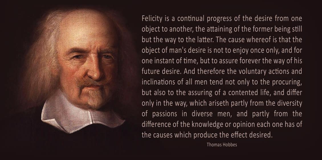
Hobbes points out that eventually, whatever I possess, others may desire. This results in violence, conflict and finally war, to which Hobbes concludes that life in a state of war would be "solitary, poor, nasty, brutish and short" (Leviathan, Thomas Hobbes 1660) If we conversely accept this as a more convincing portrayal of the state of nature, the pure liberal viewpoint simply does not seem functional. In the quest for more freedom and liberty, individuals seemingly lose many, or all, of their rights that existed in the state.

In light of this failure, a more conservative view of liberty becomes viable. If we acknowledge a state of war, then more active and strict state intervention is needed to maintain order and protect individuals from each other. This points us towards social contract theory. All of the major social contract theorists - Locke, Hobbes, Rousseau - maintain that, in order for the social contract to function, and for the state to hold legitimate political power over a society, every individual in that society must exhibit a degree of voluntarism.(An Introduction to Political Philosophy, Jonathan Wolff, 2022) Correspondingly, a key part of the social

contract is the concept of ‘tacit consent’ - the idea that in acceptance of the state’s protection and other benefits, we subjugate some of our other rights in return. Craig Carr, in explanation of tacit consent, draws parallels to the game of chess; in engaging in the game, we tacitly consent to the rules of the game without the need for explicit verbal confirmation that we are doing so.(iapss.org, Noah Busbee, 2023) This idea of a consensual state can also be reconciled with autonomy. For Locke, as seen above, humans are naturally independent and autonomous, traditionally free from any form of political power. However, since individuals volunteer themselves to the state through their consent, it can, as an artificial human construction, be married with our autonomous nature. If the state is justified, it follows that we consent to its rulings. And since the state’s personnel are elected, by the majority, on the grounds of how well they can protect their people and enforce social cohesion, it is reasonable to posit that this is its main objective. As such, perhaps we should value social order over individual rights?

“ Your freedom to swing your fist ends where my nose begins.

However, the fundamental issues arising in tacit consent, raised by David Hume, significantly destabilise the social contract. Hume clarifies that, in the absence of explicit verbal or written consent, residence in a country alone should be construed as tacit consent. Therefore he posits that the only thing that may be understood as dissent, or a lack of consent, is leaving the country. Yet in a world of nation-states this seems far too extreme as a condition to express disapproval.(Jonathan Wolff, 2022) In light of this it seems unjust to suggest that those who don’t undertake the onerous task of moving countries all together are actively consenting to the state. To come back to Carr’s chess example, Hume would condemn it as poor analogy. The simple to decision to leave the board is hardly equivalent to the decision to leave a country. It is this restriction of decision that is not synonymous with autonomy or a general view of consent, thus tacit consent should be rejected. Though this may alone, be a convincing refutation of tacit consent, it can be condemned further. Rousseau in his 1754 ‘Discourse on Inequality’ points out that every society is plagued by class and inequality, whether due to gender, race, religion or family. But if society is based on a social

contract between people who are free and equal, why on earth would people agree to a second-class status, and to their own subjugation or oppression? (Jonathan Wolff, 2022) The short response is that such a volume of people would not have, hence there cannot have been some reputable form of consent. Taken together, these criticisms mean that tacit consent fails, as do other aims to establish consent such as ‘hypothetical consent’. Consequently, social contract theory fails to establish legitimate means under which the state should hold power over its people, and its priority of social cohesion remains unjustified.

Even if liberal individualism and social contractualism are flawed, it is clear that there is a need for the individual to be free to an extent (by virtue of our autonomous nature). Yet these rights become self-defeating at the point where no social order is objectivised. In view of this, there seems to be some socially optimum distribution of rights - hence, where and what is it?

One answer was proposed by John Stuart Mill, in the form of his harm principle.(On Liberty, John Stuart Mill, 1859) In its most basic terms this principle can be verbalised as "your freedom to swing your fist ends where my nose begins". It is the idea that the rights of individuals should only be restricted when their exercise may cause harm to another individual. For instance, the principle would maintain that the act of smoking, as an expression of freedom, is perfectly fine. But at the point where this freedom causes material harm to others - the effects of passive or second-hand smoking - we must act. For example by banning

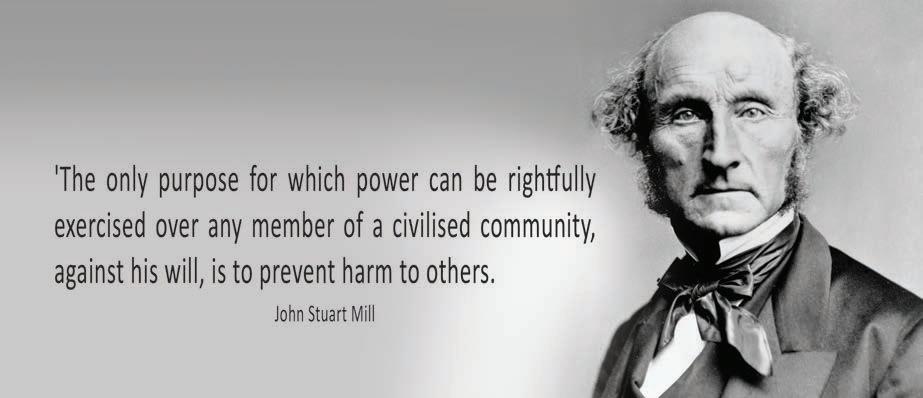
smoking in cars with children.(Children and Families Act 2014) In this way, the principle expresses that the right to self-determination is not unlimited, at some point the individual must be regulated. But it is Mill’s inability to clarify what this ‘point’ is, that ultimately renders his principle incomplete as a solution. Mill’s lack of clarity stems from his frustratingly unclear definition of ‘harm’, which he avoids almost entirely in his work. In view of this, perhaps one approach is to accept a more expansive conception of harm, that Mill intended to refer to "all bad consequences". (Harm and Mill’s Harm Principle, Piers Norris Turner, 2014)

“ By virtue of our social nature, the community (and its social customs and traditions) has a large impact on our morality and our identity.

But this seems unlikely, for Mill does express that he rejects harmful speech as something that can incite real harm - he wholly defends people’s "right to offend others". This is significant in two ways. Firstly, it evidences against a holistic interpretation of "harm" as "bad consequence" because, by specifying what he does not accept as appropriate harm, Mill clearly has a specific definition (or at least some limits) in mind. But, perhaps more importantly it shows that Mill’s harm principle may be outdated and unsuitable to apply to current society. His dismissal of psychological harm is entirely at odds with the exponential increase in mental well-being awareness that has emerged in society in the past few decades. To this end we can conclude that, both in Mill’s failure to specify a type and metric for harm, and the unsuitability of his principle in the modern landscape, the harm principle loses much of its credibility. Therefore it is not overly helpful in depicting where the line should be drawn on individual liberty.

Furthermore, the harm principle, as a key tenet of liberalism, falls foul to some criticism that may turn us to the communitarian perspective. The liberalist viewpoint, as adopted by Mill, conceives of people as isolated individuals who, in their own protected sphere, pursue their own good without any attachment to cultural rules or traditions.(Jonathan Wolff, 2022) The communitarian entirely disputes this. She argues that in reality, by virtue of our social nature, the community (and its social customs and traditions) has a large impact on our morality and our identity. For instance, in Sub-Saharan Africa, tribes following the Santeria religion regularly sacrifice animals as appeasement to their gods. In the context of their community this is not only acceptable, but cherished. In this way the communitarian critique is twofold. Firstly it asserts that the scope of human endeavour is too wide, and its moral landscape too complex, to impose upon it a singular criterion for harm. But equally it highlights the immense role of the community in shaping the morality of the Santerians, and others. Therefore perhaps instead our assessment of individual rights should revolve more around community? Thus we arrive at communitarianism.

What is unique about this theory is its roots in Aristotelian ethics. For Aristotle, what was paramount was the development of virtues within the self that would, in combination with phronesis (practical wisdom), help us to flourish and achieve eudaimonia (ultimate happiness). Similarly, communitarianism stresses these virtues, but posits they might be obtained through communal participation. For the communitarian, a person is deeply embedded into their community and so it plays a fundamental role in the shaping of virtues. As such they advocate for laws that enforce social cohesion to allow for more healthy communities that will, in turn, further develop the individual. Therefore we must not draw the line on limiting individual rights just before they cause any ‘harm’, but instead far before this. The Ultra Low Emission Zone for London, disabled parking spaces, paying taxes, all serve as examples of where the individual is restricted far before their actions threaten any real harm to others, in the name of social cohesion.

The main criticism levelled at communitarianism is that it overly romanticises the concept of community. This has some merit. Holders of this view argue that it presents the notion of community as inherently good and beneficial to all who participate in it, but that this is unrealistic. Communities can equally be a source of oppression or corruption and, just in the same way that a positive community can propel us towards flourishing, a negative community may have stunting effects on personal growth. Therefore, in instances of weak community (for at the very least we are not to believe that all communities are good), this theory seems unfeasible. However, whilst the critique is correct, it seems more of a functional weakness, an error in practice, than one that attacks the core

ideology of the communitarian. That is to say, communitarianism aims to demonstrate that a stable, productive community is essential in nurturing the individual. The presence of real-world communities that are unstable does not negate this. Instead, it may allow us to conclude that the communitarian’s critique of a liberal harm principle is apt, perhaps more attention should be attributed to a community and social order. But in practice this requires the presence of good, sustainable governance.

To strengthen the communitarian argument utilitarianism is often used as justification for the primacy of the collective. As a theory, utilitarianism prescribes moral merit to the situation in which pleasure or happiness has been maximised, often summarised as aiming to achieve "the greatest good for the greatest number"

In view of this, it is hastily assumed that a utilitarian perspective would always restrict individual freedoms to the advantage of the majority. However, in truth the situation may be far more nuanced than this, as shown in analysis of the GDL scheme explained earlier. It may in fact be the case that the intensity of the displeasure caused in young drivers, at this restriction of their freedoms, aggregates to a greater extent than the minor pleasure elicited in each of the many drivers in favour of the scheme (in the comfort that they will be marginally safer on the roads). This probes what is one of the largest objections towards the entirety of utilitarian thought, the issue of calculation. Bentham’s act utilitarianism does boast its ‘hedonic calculus’, yet this does not apply in relation to the qualitative nature of pleasure. Thus we are left with Mill’s concept of ‘competent judges’ to distinguish between and rank different types of pleasure.

Ultimately, Mill’s attempt to provide some form of additive scale is fundamentally unsatisfying. The idea that a physical panel of judges who have experienced ‘both the higher and lower pleasures’ should be assembled to deliver a verdict on considerations such as this - the balancing of pleasure attained between regulated and non-regulated drivers - is misguided. Not only is pleasure such a subjective feeling that the rulings of three individuals should not account for others who might be subject to a law. But equally we cannot always accurately recall one or both of two competing experiences, and consequently we cannot compare the two experiences.(The Competent Judge Problem, Kimberley Brownlee, 2015) Therefore utilitarianism, in application, does not augment the communitarian argument.

In closing, due to their respective limitations, none of the above theories alone can deliver a conclusion on how we should make laws. However, parts of each may be taken to create an appropriate policy. Though vague, the conditions for freedom outlined by Mill have intuitive appeal, especially if we extend his principle (from a more paternalistic perspective) to weigh the harm individuals may cause to themselves. Additionally, a communitarian perspective raises credible points about the importance of (healthy) community on the individual. If we combine Mill’s harm principle with these points, we may arrive at a good framework for law-making. If we posit an interpretation of harm as "negative effects to the social order of a community or physical/psychological damage to a person", this might provide a lens through which to recognise the fundamental importance of a community, reconciling individual rights with social cohesion.

“ A lens through which to recognise the fundamental importance of a community, reconciling individual rights with social cohesion.

BIBLIOGRAPHY

1. An Introduction to Political Philosophy, Jonathan Wolff, 2022

2. On Liberty, John Stuart Mill, 1859

3. The Competent Judge Problem, Kimberley Brownlee, 2015

4. Harm and Mill’s Harm Principle, Piers Norris Turner, Volume 124, No.2 (2014)

5. Tacit Consent: Individual Will and Political Obligation, Noah Busbee, IAPSS (2023)

6. The Guardian, 24th November, 2023

7. Leviathan, Thomas Hobbes, 1660

8. The Tragedy of the Commons, Garrett Hardin, 1968, Science Magazine

9. On the Social Contract, Jean-Jacques Rousseau, 1762

10. Social Contract Theory, Celeste Friend, Internet Encyclopaedia of Philosophy, no date

11. Strong Political Liberalism, Henrick Kugelberg, Springer Link, 2024.

COMPOSING FILM MUSIC IN THE 20 TH CENTURY

'GOLDEN AGE' STYLE

ARTS HUMANITIES

RUVIN MEDA

For his ILA project, Ruvin composed the film music to accompany a previously silent 1920s cartoon animation. This film and accompanying composition were shown at the ILA/ORIS Presentation Evening and resulted in him winning the ILA prize in the Arts/ Humanities category.

“ Film music in the Western Canon is a relatively new art form which speaks to billions of people across the world. In its mere 100 years of existence, film music has adopted a variety of musical idioms including classical, jazz,

popular music and often fusions of these styles. In my ILA, I sought to explore the music found in the Golden Age of movies, and what made them so successful and still a hugely important part of our musical culture today."

Royal Grammar School

High Street

Guildford

GU1 3BB