Journal of Automation, Mobile Robotics and Intelligent Systems, vol. 14, no. 1 (2020)

Journal of Automation, Mobile Robotics and Intelligent Systems

A peer-reviewed quarterly focusing on new achievements in the following fields:

• Fundamentals of automation and robotics • Applied automatics • Mobile robots control  • Distributed systems • Navigation

• Mechatronic systems in robotics • Sensors and actuators • Data transmission • Biomechatronics • Mobile computing

Editor-in-Chief

Janusz Kacprzyk (Polish Academy of Sciences, Łukasiewicz-PIAP, Poland)

Advisory Board

Dimitar Filev (Research & Advenced Engineering, Ford Motor Company, USA)

Kaoru Hirota (Japan Society for the Promotion of Science, Beijing Office)

Witold Pedrycz (ECERF, University of Alberta, Canada)

Co-Editors

Roman Szewczyk (Łukasiewicz-PIAP, Warsaw University of Technology, Poland)

Oscar Castillo (Tijuana Institute of Technology, Mexico)

Marek Zaremba (University of Quebec, Canada)

Executive Editor

Typesetting

PanDawer, www.pandawer.pl

Webmaster

Piotr Ryszawa (Łukasiewicz-PIAP, Poland)

Ministry of Science and Higher Education Republic of Poland

Editorial Office

ŁUKASIEWICZ Research Network

– Industrial Research Institute for Automation and Measurements PIAP Al. Jerozolimskie 202, 02-486 Warsaw, Poland (www.jamris.org) tel. +48-22-8740109, e-mail: office@jamris.org

The reference version of the journal is e-version. Printed in 100 copies.

Katarzyna Rzeplinska-Rykała, e-mail: office@jamris.org (Łukasiewicz-PIAP, Poland)

Associate Editor

Ministry of Science and Higher Education Republic of Poland

Piotr Skrzypczynski (Poznan University of Technology, Poland)

Statistical Editor

Małgorzata Kaliczynska (Łukasiewicz-PIAP, Poland) ´

Ministry of Science and Higher Education Republic of Poland

Editorial Board:

Chairman – Janusz Kacprzyk (Polish Academy of Sciences, Łukasiewicz-PIAP, Poland)

Plamen Angelov (Lancaster University, UK)

Adam Borkowski (Polish Academy of Sciences, Poland)

Wolfgang Borutzky (Fachhochschule Bonn-Rhein-Sieg, Germany)

Bice Cavallo (University of Naples Federico II, Italy)

Chin Chen Chang (Feng Chia University, Taiwan)

Jorge Manuel Miranda Dias (University of Coimbra, Portugal)

Andries Engelbrecht (University of Pretoria, Republic of South Africa)

Pablo Estévez (University of Chile)

Bogdan Gabrys (Bournemouth University, UK)

Fernando Gomide (University of Campinas, Brazil)

Aboul Ella Hassanien (Cairo University, Egypt)

Joachim Hertzberg (Osnabrück University, Germany)

Evangelos V. Hristoforou (National Technical University of Athens, Greece)

Ryszard Jachowicz (Warsaw University of Technology, Poland)

Tadeusz Kaczorek (Białystok University of Technology, Poland)

Nikola Kasabov (Auckland University of Technology, New Zealand)

Marian P. Kazmierkowski (Warsaw University of Technology, Poland)

Laszlo T. Kóczy (Szechenyi Istvan University, Gyor and Budapest University of Technology and Economics, Hungary)

Józef Korbicz (University of Zielona Góra, Poland)

Krzysztof Kozłowski (Poznan University of Technology, Poland)

Eckart Kramer (Fachhochschule Eberswalde, Germany)

Rudolf Kruse (Otto-von-Guericke-Universität, Germany)

Ching-Teng Lin (National Chiao-Tung University, Taiwan)

Piotr Kulczycki (AGH University of Science and Technology, Poland)

Andrew Kusiak (University of Iowa, USA)

Publisher:

ŁUKASIEWICZ Research Network –Industrial Research Institute for Automation and Measurements PIAP

Ministry of Science and Higher Education

Articles are reviewed, excluding advertisements and descriptions of products. If in doubt about the proper edition of contributions, for copyright and reprint permissions please contact the Executive Editor.

Republic of Poland

Ministry of Science and Higher Education Republic of Poland

Publishing of “Journal of Automation, Mobile Robotics and Intelligent Systems” – the task financed under contract 907/P-DUN/2019 from funds of the Ministry of Science and Higher Education of the Republic of Poland allocated to science dissemination activities.

Mark Last (Ben-Gurion University, Israel)

Anthony Maciejewski (Colorado State University, USA)

Krzysztof Malinowski (Warsaw University of Technology, Poland)

Andrzej Masłowski (Warsaw University of Technology, Poland)

Patricia Melin (Tijuana Institute of Technology, Mexico)

Fazel Naghdy (University of Wollongong, Australia)

Zbigniew Nahorski (Polish Academy of Sciences, Poland)

Nadia Nedjah (State University of Rio de Janeiro, Brazil)

Dmitry A. Novikov (Institute of Control Sciences, Russian Academy of Sciences, Russia)

Duc Truong Pham (Birmingham University, UK)

Lech Polkowski (University of Warmia and Mazury, Poland)

Alain Pruski (University of Metz, France)

Rita Ribeiro (UNINOVA, Instituto de Desenvolvimento de Novas Tecnologias, Portugal)

Imre Rudas (Óbuda University, Hungary)

Leszek Rutkowski (Czestochowa University of Technology, Poland)

Alessandro Saffiotti (Örebro University, Sweden)

Klaus Schilling (Julius-Maximilians-University Wuerzburg, Germany)

Vassil Sgurev (Bulgarian Academy of Sciences, Department of Intelligent Systems, Bulgaria)

Helena Szczerbicka (Leibniz Universität, Germany)

Ryszard Tadeusiewicz (AGH University of Science and Technology, Poland)

Stanisław Tarasiewicz (University of Laval, Canada)

Piotr Tatjewski (Warsaw University of Technology, Poland)

Rene Wamkeue (University of Quebec, Canada)

Janusz Zalewski (Florida Gulf Coast University, USA)

Teresa Zielinska (Warsaw University of Technology, Poland)

Journal of Automation, Mobile Robotics and Intelligent Systems

Volume 14, N° 1, 2020

DOI: 10.14313/JAMRIS/1-2020

Contents

Controller Area Network Standard for Unmanned Ground Vehicles Hydraulic Systems in Construction

Applications

Piotr Szynkarczyk, Józef Wrona, Adam Bartnicki

DOI: 10.14313/JAMRIS/1-2020/1

Application of an Artificial Neural Network for Planning the Trajectory of a Mobile Robot

Marcin Białek, Patryk Nowak, Dominik Rybarczyk

DOI: 10.14313/JAMRIS/1-2020/2

Timber Wolf Optimization Algorithm for Real Power Loss Diminution

Kanagasabai Lenin

DOI: 10.14313/JAMRIS/1-2020/3

Multi-Agent System Inspired Distributed Control of a Serial-Link Robot

S. Soumya, K. R. Guruprasad

DOI: 10.14313/JAMRIS/1-2020/4

Path Planning Optimization and Object Placement Through Visual Servoing Technique for Robotics

Application

Sumitkumar Patel, Dippal Israni, Parth Shah

DOI: 10.14313/JAMRIS/1-2020/5

Fuzzy Logic Controller With Fuzzylab Python Library and the Robot Operating System for Autonomous Mobile Robot Navigation

Eduardo Avelar, Oscar Castillo, José Soria

DOI: 10.14313/JAMRIS/1-2020/6

Toward the Best Combination of Optimization with Fuzzy Systems to Obtain the Best Solution for the GA and PSO Algorithms Using Parallel Processing

Fevrier Valdez, Yunkio Kawano, Patricia Melin

DOI: 10.14313/JAMRIS/1-2020/7

Exploring Random Permutations Effects on the Mapping Process for Grammatical Evolution

Blanca Verónica Zúñiga, Juan Martín Carpio, Marco Aurelio Sotelo-Figueroa, Andrés Espinal, Omar Jair Purata-Sifuentes, Manuel Ornelas, Jorge Alberto SoriaAlcaraz, Alfonso Rojas

DOI: 10.14313/JAMRIS/1-2020/8

Single Spiking Neuron Multi-Objective Optimization for Pattern Classification

Carlos Juarez-Santini, Manuel Ornelas-Rodriguez, Jorge Alberto Soria-Alcaraz, Alfonso Rojas-Domínguez, Hector J. Puga-Soberanes, Andrés Espinal, Horacio Rostro-Gonzalez

DOI: 10.14313/JAMRIS/1-2020/9

Application of Agglomerative and Partitional Algorithms for the Study of the Phenomenon of the Collaborative Economy Within the Tourism Industry

Juan Manuel Pérez-Rocha, Jorge Alberto Soria-Alcaraz, Rafael Guerrero-Rodriguez, Omar Jair Purata-Sifuentes, Andrés Espinal, Marco Aurelio Sotelo-Figueroa

DOI: 10.14313/JAMRIS/1-2020/10

Research Trends on Fuzzy Logic Controller for Mobile Robot Navigation: A Scientometric Study

Somiya Rani, Amita Jain, Oscar Castillo

DOI: 10.14313/JAMRIS/1-2020/11

Optimization of Convolutional Neural Networks Using the Fuzzy Gravitational Search Algorithm

Yutzil Poma, Patricia Melin, Claudia I. González, Gabriela E. Martínez

DOI: 10.14313/JAMRIS/1-2020/12

Controller Area Network Standard for Unmanned Ground Vehicles Hydraulic Systems in Construction Applications

Submitted: 15th January 2020; accepted: 30th March 2020

Piotr Szynkarczyk, Józef Wrona, Adam Bartnicki

DOI: 10.14313/JAMRIS/1-2020/1

Abstract: Unmanned vehicles occupy more and more space in the human environment. Mobile robots, being a significant part thereof, generate high technological requirements in order to meet the requirements of the end user. The main focus of the end users both in civil, and so called “defense and security” areas in the broadly defined segments of the construction industry should be on safety and efficiency of unmanned vehicles. It creates some requirements for their drive and control systems being supported among others by vision, communication and navigation systems. It is also important to mention the importance of specific design of manipulators to be used to fulfill the construction tasks. Control technologies are among the critical technologies in the efforts to achieve these requirements. This paper presents test stations for testing control systems and remote control system for work tools in the function of teleoperator using the CAN bus and vehicles which use hydrostatic drive systems based on the Controller Area Network (CAN) standard. The paper examines the potential for using a CAN bus for the control systems of modern unmanned ground vehicles that can be used in construction, and what limitations would possibly prevent their full use. It is exactly crucial for potential users of unmanned vehicles for construction industry applications to know whether their specific requirements basing on the tasks typical in construction [9] may be fulfilled or not when using the CAN bus standard.

Keywords: CAN bus, control systems, unmanned ground vehicles – mobile robots, hydrostatic drive systems, construction equipment

1. Introduction

Unmanned construction systems could be used to perform emergency countermeasure work and restoration work at disaster sites but also to increase safety at ordinary construction sites. Unmanned construction was used in civil engineering work for the first time in Japan in 1969 when an underwater bulldozer was used to excavate and move deposited soil during emergency restoration work at the Toyama Bridge that have been blocked by the Joganji River disaster [9]. There were

also some concepts to implement the remote controlled systems into manned platforms [6].

The executions can be categorized as emergency and restoration works [9]. It creates possibilities to define some principal types of hazardous tasks typical in construction for which unmanned vehicles could be used. There can be specified following works: rock removal work (excavation, loading, transporting), structure demolition and removal work (crushing and pulverizing concrete and cutting steel reinforcing bars, loading and transporting the products), large sandbag placing work (transporting and placing), concrete block work (removing obstructions, leveling ground, placing), temporary road work (cutting, filling and compaction), erosion and sediment control dam work (excavation, embanking, backfilling, compaction, pouring concrete), watercourse work (excavation, pouring concrete, placing foot protection blocks), tree felling work (cutting, stumping, transporting), Reinforced Cement Concrete RCC work (transporting, spreading and leveling, compaction, spraying, laitance removal), ready-mix concrete work (installing form materials, pouring and compacting concrete) and soil form work (excavation, loading, transporting, removing form materials) [9]. The specificity of the tasks performed by today’s unmanned ground vehicles, the ability to use them for hazardous construction tasks creates demanding requirements for both their drive, control, communication and navigation systems. The basic requirement for drive systems being discussed in this paper is to provide high mobility and control precision in the conduct of reconnaissance and rescue missions, as well as to achieve high power and torque for actuators of work tools. The progressive development of hydraulic components (their reliability and susceptibility to control) are the reasons why hydrostatic drive systems are increasingly used in solutions for drive systems of modern unmanned land platforms which offer both very good traction parameters of a vehicle and sufficiently large forces for their work tools which is crucial in case of construction machinery. An advantage of such solutions is relatively long operating time of these platforms limited only by the capacity of their fuel tanks (supplying combustion engines), as opposed to robots driven by electric propulsion systems whose working time is limited by the capacity of battery cells. Recreating readiness for reuse is at the present stage of cell technology development significantly longer than the process of refuelling. Full

utilization of the potential of these drive systems is only possible where modern control systems are introduced. Due to the principal categories of work performed the method described in [9] there are two examples of unmanned ground vehicles presented in this paper when this is a problem in the execution of construction tasks like rock removal work (loading, transporting), structure demolition, large sandbag placing work (transporting and placing), some concrete block and tree felling work.

Robert Bosch GmbH commenced its development of a Controller Area Network (CAN) in 1983. A Controller Area Network (CAN bus) is generally a vehicle bus standard designed to allow microcontrollers and devices to communicate with each other in applications without a host computer [7]. Unlike a traditional network such as USB or Ethernet, CAN does not send large blocks of data point-to-point from node A to node B under the supervision of a central bus master [8]. In this paper the main focus is on the applications of CAN systems for controlling hydraulic drives of modern unmanned ground vehicles for use in construction.

The CAN technology officially was introduced in 1986 at the Society of Automotive Engineers (SAE) Congress in Detroit, Michigan. The first CAN commercial solution appeared on the market in 1987, produced by Intel & Philips [3]. In 1991, Bosch released version 2.0 of CAN. Bosch first developed the CAN controller technology for use in a vehicle network in 1985 [3]. The advent of new technology for the control of hydraulic components – the CAN-bus system in its mobile version opened a new, long-awaited opportunities in the field of tools and work process control in machines equipped with hydrostatic drive systems. While descriptions of applications of this technology for drives other than hydraulic are available [1,2,3], the knowledge about the applications of CAN systems for controlling hydraulic drives is limited.

That is why the control system for an unmanned land platform based on a CAN bus standard has been developed and results of analysis to answer the scientific question what are opportunities and limitations for the use of such a standard in hydrostatic drive systems for unmanned construction machinery and how this research will contribute to determining whether the use of CAN-bus systems is indeed feasible in such machinery is presented in this paper.

2. Test Station for Hydrotronic Tests of Drive Trains Operating in the CAN-bus System

For the purposes of identifying the limitations and possibilities of implementation of the CAN-bus technology in mobile robot control systems and modern engineering machinery, two test stations were built at the Institute of Robots and Machine Design, Faculty of Mechanical Engineering, Military University of Technology (Figs. 1,2) at which actuators for the hydrostatic drive system were tested, controlled with the use of hydraulic distributors equipped with electronic modules cooperating with the CAN bus.

The basic elements of the stations are five working ports hydraulic valves (1 – Fig. 1) allowing the control of all movements of the work tools, consisting of single PVG32 type sections and operating in the LS (Load Sensing) system. The movement of hydraulic valves spools is controlled via PVED-CC electronic modules which are designed to work using the CAN-bus protocol. The PVED-CC Series 4 is an electrohydraulic actuator which consists of an electronic part and a solenoid H-bridge. The PVED-CC Series 4 transforms a command signal transmitted on a CAN bus into a hydraulic action by applying pressure acting on the end of the spool [11]. The individual coils are activated using remote control panel joysticks (2 – Fig. 1) generating analogue and digital control signals or the test station for testing the remote control system for work

Fig. 1. Test stations for testing control systems using the CAN bus: 1 – hydraulic valve with electronic CAN-bus modules, 2 – remote control desktop, 3 – hydraulic power unit, 4 – work tools

tools in the teleoperator function based on the CAN bus (Fig. 2). In this case the vision system provides a panoramic view of the surroundings, and a camera mounted in the manipulator holder (a – Fig. 2) allows for the identification and analysis of picked objects.

Below, (Fig. 3) there is presented the scheme of main control desktop as a component of the remote control station. Whereas on Fig. 4 the scheme of platform on-board control system is presented.

Beside the tests of functionality and effectiveness of manipulator operations, the measurements of its maximum load for different manipulator lift range were done at the test station (Fig. 5). The measurement system is based on force sensor CL-14d (1 – Fig. 5) equipped with amplifying system CL 71, ZEPWN (2 – Fig. 5). Additionally, the load force was measured using dynamometer 9016 APU-20-2-U2 (3 – Fig. 5). The results of tests were recorded with the use of ESAM TRAVELLER Plus data acquisition system.

Fig. 5. Test station for measurement of load force of engineering support robot manipulator (description in the content of the text above)

The value of manipulator loads were recorded both for different manipulator lift ranges and for different its configurations but the same lift range. There, on Fig. 6 the exemplary manipulator configurations for lift range of 2100 mm were presented. The achieved results of the tests are presented at the Fig. 7.

These results approved manipulator capabilities to lift the loads of 500 N for maximum lift range of 4700 mm and possibility to lift the load of 13 kN for lift range of 2100 mm and optimal manipulator configuration.

These tests allowed to define the maximum value of manipulator loads from the point of view of its kinematics and parameters of hydrostatic drive line controlled with the use of Controller Area Network Standard system.

Mutual communication between elements of the control system is carried out using microcontrollers of the PLUS+1 system. CAN-based PLUS+1 microcontrollers are the brains behind intelligent vehicle control. Swiftly programmable to its specific requirements [12].

Fig. 2. Test station for testing the remote control system for work tools in the function of teleoperator (a), based on the CAN bus of Engineering support robot EOD/IED “Marek”

Fig. 3. Scheme of control desktop of the remote control station

Fig. 4. Scheme of platform on-board control system

3. Unmanned Land Platform Controlled Based on a CAN Bus

As part of research into the possibility of using the CAN bus to control unmanned construction vehicles a light high mobility unmanned vehicle was developed with hydraulic coupling equipped with a hydrostatic drive in which a turn is accomplished by changing the angle of the relative positions of two parts of the vehicle connected by the coupling (Fig. 8). The high mobility of the vehicle is provided by a flexible crawler track where tracks are driven independently by four gerotor motors. Control of the vehicle is realized on the basis of hydraulic valves equipped with electronic modules operating in the CAN system which allows both – changing the speed of the vehicle and its direction of movement. The main drive unit of the vehicle (a combustion engine) and the hydrostatic drive system make it possible for the vehicle to be equipped with additional work tools utilizing the hydraulic energy of the operating fluid or electricity generated by on-board sources of energy. It is therefore possible to mount all kinds of self-levelling platforms, manipulators, cutting saws, hydraulic cutters, etc. on the vehicle. All such components can also be adapted for remote control.

There will be conducted tests to reach more data for quantitative anaylysis on the base of this platform. It will be also part of Validation&Verification tests for simulation models of platform and its drive line components equipped with electronic modules operating in the CAN system.

4. CAN-Bus in Remote-Controlled Engineering Robots for the Modern Battlefield

Other two designs which use the CAN bus in drive control and work tool control systems are engineer-

Fig. 6. Exemplary manipulator configurations for lift range of 2100 mm

Fig. 7. The graph of engineering support robot manipulator load

Fig. 8. Unmanned land platform with control based on a CAN: 1 – hydraulic valve, 2 – electronic CAN-bus modules

ing support robots Boguś and Marek (Figs. 9 and 10). Boguś is designed to perform tasks related to the supply of field work crews operating in a difficult to access areas. It can also act as a carrier of various types of reconnaissance or construction task systems like rock removal work (loading, transporting), structure demolition, large sandbag placing work (transporting and placing), some concrete block and tree felling work. The robot is built as a two-part structure, with a hydraulic coupling connecting the two parts. The power unit is a turbocharged diesel engine with a power of about 60 kW, the drive system is 10x10 (the first part – 6x6, second part – 4x4), transmission – mechanical and hydrostatic with interaxial lock. Independent hydro-pneumatic suspension with lockable front wheels and an lever-articulated turn system.

The time of operation has been determined to be not less than 8–10 hours. With the use of the two-part system with a specially designed hydraulic coupling it is possible to obtain a turning radius of about 4 m. This solution makes it possible to clear ditches with a width of 1 m and hills with a slope of 45°. A hydraulic fork lift mounted on the second part is designed for self-loading and self-unloading of objects (e.g. a standard pallet sized 2.5x1 m) with a weight up to 2000 kg, from storage level and from trucks.

The main dimensions of the robot are: length 7-8 m, width approx. 2.1 m, while the basic parameters are: curb weight approx. 4000 kg, load capacity 2000 kg + 1000 kg, maximum speed 30–40 km/h.

“Marek” (Fig. 10) is a 6-wheeled vehicle with a weight of approx. 3200 kg powered by a turbo-

Fig. 10. Engineering support robot EOD/IED “Marek”

Fig. 9. Engineering support robot “Boguś”

charged diesel engine with a power of approximately 60 kW. A 6x6 drive system with independent hydro-pneumatic suspension was proposed as part of this solution. Adequate traction properties have been achieved by using a hydrostatic drive system with a side lock and an interaxial lock, in which each wheel is independently driven by a gerotor motor. The side turn system makes the vehicle very manoeuvrable and allows turning with a zero turning radius, around the vertical axis of the robot. The robot is equipped with a manipulator with a special gripper and an openwork bucket loader. Work tools of the machine are also driven using the hydrostatic drive system.

The kinematics of the manipulator and its design are to provide the ability to pick from a roadside ditch or from a cavity in the ground:

– a load up to 250 kg and with a diameter of 600 mm (e.g. a barrel, aerial bombs, artillery ammunition, missiles);

– small objects with a diameter of less than 100 mm (e.g. grenades);

– prefabricated concrete elements, debris and boulders weighing up to 250 kg;

steel and wood structural elements (rods, sections, beams, boards, timber).

Like in the case of “Boguś” robot, “Marek” is designed to perform tasks related to the supply of field work crews operating in a difficult to access areas. It can also perform construction task systems like rock removal work (loading, transporting), structure demolition, large sandbag placing work (transporting and placing), some concrete block and tree felling work.

In addition to the manipulator, the robot is equipped with a lift and loader tools with a quick coupler for linking various different tools. The main tool is an openwork bucket capable of digging loose soil (category I and II) and separating from it objects with a minimum diameter under 50 mm, and lifting/ turning over bulky objects, digging out subsurface objects, anchoring – in order to increase the forces achieved by the manipulator – and as a support to increase robot stability. With the lift, it is to be capable of moving (lifting, pushing) concrete blocks, cave-ins, tree trunks, barriers, steel trusses etc. with a mass of up to 2000 kg. The proposed design solutions ensure 8-10 operating hours of the robot.

In both cases, the drive systems of the vehicles are controlled using a CAN bus based on the elements of the PLUS+1 system. Independent drivers are also used in the ride, work tool, hydraulic coupling and active hydropneumatic suspension control systems. The use of hydraulic gerotor motors designed to work on a CAN bus has made it much easier to control them in terms of obtaining the maximum values of torque on individual wheels, and the process of controlling the hydropneumatic suspension ensured continuous contact of drive wheels of the vehicle with the ground.

Another example could be the Expert robot [15]. A potential application of the Expert robot is to in-

11. Two PIAP robots performing construction tasks: a) Ibis/RMF with hydraulic cutter, b) RMI turning off the valve to demonstrate wrist infinite rotation functionality

spect critical infrastructure including dangerous places being results of earthquake or any other disasters. It was also used to set explosives in the building destined for demolition. Expert was designed for use in small spaces where the larger Inspector robot [10] would not be able to enter. Such confined spaces include small rooms in buildings.

The robot is powered from gel batteries permitting operation for 3 to 8 hours, or through a cable from 230V mains. Expert features a significant operating range of the arm, almost 3 m. The manipulator has six degrees of freedom plus the clamp of gripper jaws, each step being independent. The robot is equipped with six cameras, four of them on the mobile base of the robot. Two cameras are placed on front tracks and look in opposite directions to the sides; their location over the ground changes with the setting of the tracks.

The other examples are Ibis/RMF [13] and RMI [14] shown in Fig. 11. The first one is six-wheeled chassis robot with independent drive of each wheel that allows to operate in challenging and varied terrain. IBIS® is a fast robot (10 km/h). Special design of mobile base suspension ensures optimum wheel contact with the ground. Manipulator with extendable arm ensures a large reach (over three meters) and a high range of motion in each plane. It is possible to equip the manipulator in different tools including construction. The second one PIAP RMI® – Mobile Robot for Intervention is a tracked vehicle which can replace or assist humans in the most dangerous tasks. It’s dimensions and drive system allow to carry out activities both indoors and in difficult field conditions performing different task including construction.

Fig.

5. Testing Methodology

Testing hydraulic systems can be carried out using both the quantitative method [4] and the qualitative method [5]. At this stage, using the results obtained from tests conducted with the assumed methodology, it is possible to perform a qualitative analysis but some quantitative results are presented at Fig. 7. These will be the issue for the next step tests.

While these test methods have been developed to enable answering the research question: whether there is a possibility of using a CAN bus for the control systems of modern unmanned ground vehicles, and whether certain limitations do not prevent their full use being focused on the quantitative rather then qualitative analysis.

The test subjects were:

– two test stations (Figs. 1,2), at which actuators for the hydrostatic drive system were tested, controlled with the use of hydraulic valves equipped with electronic modules cooperating with the CAN bus;

– light high-mobility unmanned vehicle with a hydraulic coupling, equipped with a hydrostatic drive (Fig. 8);

– engineering support robots Boguś (Fig. 9) and Marek (Fig. 10).

It was assumed that the tests would focus on issues relating to the areas of both the possibilities and limitations resulting from the use of systems based on the CAN standard.

The abovementioned subjects were tested in order to obtain analytical material for such research areas as:

– requirements for systems based on the components of the CAN standard;

– operational reliability of both the actuator elements and control;

– susceptibility of unmanned land vehicles to control;

– precision of control and system diagnosis;

– creating complex, multifunctional control systems;

– creating complex, multifunctional diagnostic systems;

– implementation of CAN systems for autonomous unmanned land platforms;

– application of CAN standard components in existing mobile robot solutions;

– costs.

Based on the results of tests carried out on real objects qualitative analytical tests were carried out, the

Tab. 1. Analysis of possibilities for the use of CAN bus in control systems for mobile robots

No. Possibility

1. Operational reliability where used for both actuators in hydrostatic drive systems and their control systems

Description of possibility

The CAN bus is a solution with very high operational fail-safety, reliability and low interference potential.

RED CAN used as a closure of the bus ensures increased, improved reliability in the case of partial failure of the bus.

2. Susceptibility to control, including remote control CAN actuators enable their easy configuration and interference in control characteristics.

3. Precision of control – particularly important for tasks requiring high precision, e.g. identification, picking and neutralization of hazardous charges

4. Creating complex, multifunctional control systems

5. Creating complex, multimetric diagnostic systems

6. Implementation of CAN systems for autonomous unmanned land platforms

Control procedures generated by CAN controllers bring a new quality – an innovative approach to control logic based on intuitive control.

The application of the CAN technology enables the implementation of a multiprocessor, multi-controller process.

The use of the CAN technology makes it possible to implement a multi-processor, multi-controller process supported through the use of CAN sensors capable of selfcalibration (intuitive control system). It helps diagnose hydrostatic drive systems and their control systems.

The complexity of the structures of autonomous systems enforces the implementation of the CAN technology. In their control systems there is an increasing number and volume of transmitted information. Given the current technological possibilities for its transmission to and from the system, the use of the CAN technology enables the follow-up of the control system and actuating system. Placing on the market intuitive programming systems for controllers generating control signals to the CAN bus also results in the emergence of friendly, intuitive user interfaces (Human-Machine Interface, HMI).

7. Flexible design

8. Cost reduction

Application of the CAN technology allows the introduction of modular design, in which even the user can make changes to the configuration (e.g. add or remove equipment of the vehicle fitted with CAN-bus nodes). There is also the susceptibility of the design to be extended by functionalities which were initially unforeseen.

The costs of application of professional systems of connectors and cables often add up to considerable amounts. The use of CAN significantly reduces the number of cables.

No. Limitation

1. Need to change the approach to the design and construction of systems with the use of control systems based on the CAN bus

2. Adapting existing unmanned land vehicles for the use of the CAN bus

3. Need to change the concept of diagnosing the status of the robot

4. Costs

Description of limitation

Implementation of control systems based on the CAN bus requires unmanned vehicles to be equipped with actuators designed to be controlled by control components operating based on the concept of CAN systems. This process should take place as early as the design phase.

The use of CAN system components gives rise to the need to redesign both the control system and the actuator system.

The introduction of systems to diagnose the status of a robot based on the use of the CAN standard necessitates the need to use appropriate sensors and requires the use of specialized diagnostic equipment.

A higher price of components made in the CAN standard as compared to the previously used components.

results of which have been tabulated and discussed, indicating both the possibilities and limitations of the use of systems operating in the CAN standard.

Then conclusions were formulated focusing on answering the research question posed in this paper.

6. Test Results and Analysis

Analysis of the results of analytical research was carried out based on the results of tests carried out in accordance with the developed methodology, using two testing stations and three unmanned ground vehicles indicated in the previous section, focusing on the research areas identified therein. The results of the analytical tests are given in Tables 1 and 2.

Table 1 identifies six areas of possible use of CAN bus in control systems for mobile robots.

The analysis of the results of analytical research shows that the CAN bus is a solution with very high operational fail-safety, reliability and low interference potential. The use of the Controller Area Network (CAN) protocol analyzer (RED CAN) as a closure of the bus offers increased and improved reliability in the case of partial bus failure, which is very important from the point of view of the continuity of control, particularly for remote control. In previous developments of this technology, problems with CAN were noted which were associated with the inability to obtain a response to information in real time, in particular to information with a lower priority [2]. Currently, the CAN protocol is an asynchronous serial communication protocol compliant with the ISO standard 11898 (11898-1 [3]), widely used due to its real-time operation, reliability and compatibility with other devices [1] including, as was noted in the course of the testing in question, components of hydrostatic drive systems and control systems of unmanned ground vehicles. The protocols of top level are DeviceNet protocols, open CAN, J1939 [3]. Therefore, CAN actuators currently used for these applications enable their easy configuration and interference in control characteristics.

In the case of unmanned ground vehicles, susceptibility to control and precision of control are particu-

larly important for tasks requiring high precision, e.g. dealing with hazardous materials on project sites, inspect critical infrastructure including dangerous places being results of earthquake or any other disasters is very important. Testing vehicles with a hydraulic drive system, where the vehicle is controlled using hydraulic distributors equipped with electronic modules operating in the CAN system, they allow their easy configuration and interference in control characteristics. On the other hand, control procedures generated by CAN controllers bring a new quality allowing the use of an innovative approach to control logic which is based on intuitive control.

The ability to create multifunctional control systems, multimetric diagnostic systems is essential when using the CAN technology for autonomous unmanned land platforms. In their control systems there is an increasing number and volume of transmitted information. Given the current technological possibilities for its transmission to and from the system, the use of the CAN technology enables the follow-up of the control system and actuating system. Placing on the market intuitive programming systems for controllers generating control signals to the CAN bus also results in the emergence of friendly, intuitive user interfaces (Human-Machine Interface – HMI). It would also not be possible to develop the subsequent levels of autonomy without the ability to implement a multi-processor, multi-controller process supported through the use of CAN sensors capable of self-calibration (intuitive control system). The use of the CAN technology helps diagnose hydrostatic drive systems and their control systems.

Table 2 identifies four areas of limitations for the use of the CAN bus in control systems for mobile robots.

The results of research show that most of the limitations are due to the need to change the philosophy of designing new solutions for unmanned ground vehicles, in this case in the field of hydrostatic drive systems and their control systems with the use of control systems operating on the basis of the CAN systems concept. On the other hand, when using this technology for existing mobile robots the use of CAN system

Tab. 2. Analysis of limitations to the use of CAN bus in control systems for mobile robots

components gives rise to the need to redesign both the control system and the actuator system. In both cases, it is necessary to change the concept of diagnosing the status of the robot. This forces the need to use appropriate sensors and requires the use of specialized diagnostic equipment, but it is very important especially when achieving higher levels of autonomy of the vehicles.

The last of the analyzed areas was the cost of implementing this technology for unmanned ground vehicles. At the current stage of development and application of this technology in the field of hydrostatic drive systems and their control systems for mobile robots, the higher price of components made in the CAN standard as compared to the previously used components can give rise to some budgetary constraints.

7. Conclusion

Many areas of the possibilities and limitations of the use of the CAN technology for hydrostatic drive systems and control systems of unmanned ground vehicles overlap with other areas of application of this technology. However, unmanned ground vehicles are characterized by a specificity resulting from the range of their tasks and how they are executed.

The developed methodology has enabled carrying out analysis in order to answer the research question: whether there is a possibility of using a CAN bus for the control systems of modern unmanned ground vehicles. As a result of the carried out analytical research their possibilities and limitations have been determined. The latter do not prevent the use of this technology for hydrostatic drive systems and thereby for control systems of mobile robot with this kind of drive.

The need for precise control of the new generation of engineering machines, the possibility of interfering with their control procedures online and the need for continuous diagnostics of work processes are now becoming a global standard. Its fulfilment, however, requires the knowledge of the capabilities and limitations of the existing systems. This knowledge is currently possessed by the few companies working on new technologies in this area, and there are no scientific publications on this subject. The use of the new control technology, the CAN bus system, for the implementation of technological tasks by today’s unmanned ground vehicles can significantly affect both the efficiency of their work processes and operator comfort when using remote control. Therefore, identification of these problems, learning about the possibilities and identification of limitations to the control of hydrotronic systems in the CAN-bus system of mobile robots, determination of the possibilities for the use of the CAN-bus technology for the remote control of work tools has allowed us to implement state-ofthe-art drive systems for unmanned ground vehicles – guaranteeing the high quality of their performed technological tasks, as well as the safety of these tasks in hazardous areas.

This is the purpose of vehicles and machines with hydrostatic drive, controlled based on the CAN bus. The conducted research shows that it is possible to use the CAN bus to control of drive and work tools of unmanned vehicles. Its results to date in such research areas as: requirements for systems based on the components of the CAN standard, operational reliability of both the actuator elements and control, susceptibility of unmanned land vehicles to control, precision of control and system diagnosis, creating complex, multifunctional control and diagnostic systems, implementation of CAN systems for autonomous unmanned land platforms, application of CAN standard components in existing mobile robot solutions and costs have made it possible to carry out qualitative analysis of possibilities and limitations for the use of can bus in control systems for mobile robots .

Implementation of the next phase of research consisting of unmanned platforms being equipped with sensors to measure parameters resulting from defined methodology will allow performance of a quantitative analysis, which should answer the next research question: what are the quantitative differences between using classical components and control systems for vehicles with a hydrostatic drive system, and the application of components of drive system and vehicle control based on hydraulic valves equipped with electronic modules operating in the CAN system. A future approach will also involve carrying out tests of manned vehicles in which remote control systems have been implemented [6]. These tests will be also part of Validation & Verification tests of simulation models, both some platforms described in this paper and its drive line components controlled based on a can bus.

AUTHORS

Piotr Szynkarczyk – ŁUKASIEWICZ Research Network – Industrial Research Institute for Automation and Measurements PIAP, Al. Jerozolimskie 202, 02486 Warsaw, Poland.

Józef Wrona* – Military University of Technology (WAT), ul. gen. Sylwestra Kaliskiego 2, 00-908 Warsaw, Poland, e-mail: jozef.wrona@wat.edu.pl.

Adam Bartnicki – Military University of Technology (WAT), ul. gen. Sylwestra Kaliskiego 2, 00-908 Warsaw, Poland.

*Corresponding author

R EFERENCES

[1] S. K. Gurram and J. M. Conrad, “Implementation of CAN bus in an autonomous all-terrain vehicle”. In: 2011 Proceedings of IEEE Southeastcon, 2011, 250–254, DOI: 10.1109/SECON.2011.5752943.

[2] W. Baek, S. Jang, H. Song, S. Kim, B. Song and D. Chwa, “A CAN-based Distributed Control System for Autonomous All-Terrain Vehicle (ATV)”, IFAC Proceedings Volumes, vol. 41, no. 2, 2008, 9505–9510, DOI: 10.3182/20080706-5-KR-1001.01607.

[3] V. D. Kokane and S. B. Kalyankar, “Implementation of the CAN Bus in the Vehicle Based on ARM 7”, IJRET: International Journal of Research in Engineering and Technology, vol. 4, no. 1, 2015, 29–31.

[4] “Introduction to Quantitative Research Methods”. M. T. Smith, https://people.kth.se/~maguire/courses/II2202/ii2202_intro_to_quantitative_methods_2012_MTS_Lecture5a.pdf. Accessed on: 2020-05-28.

[5] “Introduction to Qualitative Research”. www. blackwellpublishing.com/content/BPL_Images/ Content_store/Sample_chapter/9780632052 844/001-025[1].pdf. Accessed on: 2020-05-28.

[6] A. Bartnicki, M. J. Łopatka, L. Śnieżek, J. Wrona and A. M. Nawrat, “Concept of Implementation of Remote Control Systems into Manned Armoured Ground Tracked Vehicles”. In: Innovative Control Systems for Tracked Vehicle Platforms, 2014, 19–37, DOI: 10.1007/978-3-319-04624-2_2.

[7] “History of the CAN technology”, CAN in Automation (CiA), www.can-cia.org/can-knowledge/can/can-history. Accessed on: 2020-06-19.

[8] S. Corrigan, Introduction to the Controller Area Network (CAN), Application Report, SLOA101B, Texas Instruments, 2002.

[9] Y. Ban, “Unmanned Construction System: Present Status and Challenges”. In: Proceedings of the 19th ISARC, 2002, 241-246, DOI: 10.22260/ISARC2002/0038.

[10] “INSPECTOR: robot for inspection and intervention”. Industrial Research Institute for Automation and Measurements PIAP, http://antiterrorism.eu/wp-content/uploads/inspector-en. pdf. Accessed on: 2020-05-28.

[11] “PVED-CC Series 4 Electrohydraulic Actuator Technical Information Manual”. Danfoss, https://assets.danfoss.com/documents/ DOC152886483924/DOC152886483924.pdf. Accessed on: 2020-05-28.

[12] “PLUS+1® MC microcontrollers”. Danfoss, https://www.danfoss.com/en/products/electronic-controls/dps/plus1-controllers/plus1-mc-microcontrollers/#tab-overview. Accessed on: 2020-05-28.

[13] “IBIS®: robot for pyrotechnic operations and reconnaissance”. Industrial Research Institute for Automation and Measurements PIAP, http://antiterrorism.eu/wp-content/uploads/ ibis-en.pdf. Accessed on: 2020-05-28.

[14] “RMI: mobile robot for intervention”. Industrial Research Institute for Automation and Measurements PIAP, http://antiterrorism.eu/wp-content/uploads/piap-rmi-en.pdf. Accessed on: 2020-05-28.

[15] “EXPERT: neutralizing and assisting robot”. Industrial Research Institute for Automation and Measurements PIAP, http://antiterrorism.eu/ wp-content/uploads/expert-en.pdf. Accessed on: 2020-05-28.

Application of an Artificial Neural Network for Planning the Trajectory of a Mobile Robot

Submitted: 08th November 2019; accepted: 30th January 2020

Marcin Białek, Patryk Nowak, Dominik Rybarczyk

DOI: 10.14313/JAMRIS/1-2020/2

Abstract: This paper presents application of a neural network in the task of planning a mobile robot trajectory. First part contains a review of literature focused on the mobile robots’ orientation and overview of artificial neural networks’ application in area of robotics. In these sections devices and approaches for collecting data of mobile robots environment have been specified. In addition, the principle of operation and use of artificial neural networks in trajectory planning tasks was also presented. The second part focuses on the mobile robot that was designed in a 3D environment and printed with PLA material. The main onboard logical unit is Arduino Mega. Control system consist of 8-bits microcontrollers and 13 Mpix camera. Discussion in part three describes the system positioning capability using data from the accelerometer and magnetometer with overview of data filtration and the study of the artificial neural network implementation to recognize given trajectories. The last chapter contains a summary with conclusions.

Keywords: artificial neural network, mobile robot, machine vision

1. Introduction

The idea of artificial neural networks (ANN) was taken from natural neurons, which are the basic elements of the nervous system of living organisms, including humans. Neural networks has become the subject of research for various specialties and fields of science, discovering newer and more creative forms of their use. Researchers around the world are developing ANN capabilities, striving to achieve efficiency comparable to living organisms. The number of neurons used is the main comparative scale in these studies. However, unlike real counterparts, they do not transfer signals only, but allow their processing, e.g. by making calculations. The ANN’s ability to carry out its tasks is determined by the learning process. The combination of ANN issues and mobile robotics is one of the main currents in the development of modern mechatronics. Planning the trajectory of a mobile robot using SSN requires an approach to two issues.

The first is the network itself, which is to recognize the given trajectory. The second is a robot that maps it, which must determine its location in space in a specific way, while avoiding obstacles.

1.1. Orientation of Mobile Robots in Space

Autonomous navigation of mobile robots is one of the main problems faced by their designers, mainly due to the problem of its definition in an unspecified area. To accomplish this task, it is necessary to equip the mobile robot with the sensors to collect data about the environment and its location. Their selection is related to the tasks the robot will perform, and thus the positioning accuracy and type of obstacles, which are mainly characterized by a specific geometry or color are mandatory to be known. Low cost solutions are based on Ultrasonic Sensors (US). The main disadvantages of proposed system was the angle restrictions at which the sound wave falls on the detected surface of the obstacle and the material of which it is made [1]. Nevertheless, they are one of the basic types of sensors used in mobile robots, especially for the implementation of obstacle avoidance tasks [2] and in indoor tasks [3]. It is also possible to track ultrasonic beacons in real time [4] by becoming a transmitter looking for receivers or being a receiver itself. Second popular device is infrared sensor (IR). Characteristic features of obstacles force adjustment of their recognition strategy. The rational approach is to use both ultrasonic and infrared sensors, due to the possibility of mutual complementarity in the detection capabilities [5]. In the case of small mobile robots, the basic environment detection system includes elements such as ultrasonic sensors, infrared sensors, cameras and microphones [6,7]. Global Positioning System (GPS) allows locating receivers based on determining their distance from satellites (at least three) in which they are located, giving data in a quasi-spherical coordinate system (due to the fact that the Earth is not an ideal sphere), which are geodetic coordinates such as: geodetic latitude and longitude and ellipsoidal height or in geographical coordinates: longitude and latitude [8]. The GPS system is designed to locate objects on a larger scale of displacements, expressed in kilometers (square kilometers). That is why it works well with vehicles covering considerable distances in a relatively short time, moving at a much higher speed than mobile robots, being able at the same

time to predict its location by projecting the vehicle’s direction of movement onto a road map. Robot displacements are much smaller and therefore require greater accuracy [3].

To create maps of the environment, LiDAR sensors are used. They allow to detect objects by measuring laser pulses which are proportional to their distance from the source. For example, determining the position of a robot by measuring distance and angle relative to another robot, using measurements obtained from raw data provided by two laser rangefinders in a 2D plane [9], positioning and orientation of the mobile robot in 3D space, using a laser head measuring the position relative to photoelectric reference points, deployed in the room [10] or the use of an industrial laser navigation system to collect information about the distance between the rotating measuring head and the markers located on the perimeter of the laser beam plane in the area of robot operation [11]. The practical application of LiDAR technology can be autonomous navigation of an agricultural robot in conditions without access to GPS-based solutions [12] or mapping of the environment, through its hybrid representation and robot location [13].

One of the popular devices used to navigate mobile robots has become the Microsoft Kinect system, which is an accessory for the Xbox game console [14]. It’s a vision-based system. Kinect is a common tool for navigating a mobile robot, enabling it to avoid obstacles while supplying data, e.g. to an artificial neural network, which deals with environmental recognition and makes decisions about choosing a specific path [14, 15]. An additional advantage of vision system was the creation of algorithms that allow simultaneous localization and building of a map, such as SLAM (Simultaneous Localization and Mapping) [16] and all related solutions such as S-PTAM (SLAM – Parallel Tracking and Mapping) [17]. Solutions for locating robots in a confined space include those based on all kinds of mutual radio communications between mobile robots or reference points. Simple location methods using a local wireless network allow the determination of Euclidean distance between the sample signal vector and references stored in the database [18]. Another use of a wireless network is the use of defined access points to locate an object by measuring signal strength using a compressive sampling theory [19], it enables effective reconstruction of signals from a small amount of data [20]. The considerations to date on the ways of navigating mobile robots are based on different ways of obtaining location data. As previously noted, popular space location and orientation systems such as GPS exhibit lower indoor efficiency. In turn, solutions based on defined reference points limit the robot to operate only in space covered by them. Especially when operating indoor, they give way to other information-based solutions from magnetometers, accelerometers and gyroscopes [21].The data obtained by these sensors can mutually compensate for their errors [22], and in some cases inertial navigation may be valuable [23]. It is based on

continuous assessment of the object’s position using data from susceptible sensors (such as gyroscope and accelerometer) in relation to the initial position. Not least is also the approach to control the motor drives in accordance with terrain environment [24].

1.2. Artificial Neural Networks

Artificial neural networks have been a field strongly developed over the years among other things in the form of so-called open source projects. Currently, TensorFlow libraries, designed by Google, in November 2015 are one of the most frequently used open source libraries. The vast majority of C ++ were used to write these libraries. Moreover they can use GPU (Graphics Processing Unit) for calculations, what significantly speeds them up. Another advantage of this software is the ability to work on less efficient Raspberry Pi devices or smartphones. ANNs are very often used for all sorts of image classification. Neural networks presented at the International Conference on New Trends in Information Technology[25] is a good example. They can recognize both Arabic script and faces. The architecture of the text recognition network is based on four hidden layers, and its diagram is shown in Fig. 1.

This network was taught based on numbers from zero to ten in 60,000 samples. The image fed at the entrance had a size of 28x28 pixels, which gives a total of 784 pixels for each sample. The value of the number of pixels determines the number of network input neurons shown in Fig. 1. The learning algorithm was based on the back propagation method of the network response error. The network designed in this way has the ability to recognize the images given on its input with an efficiency of 98.46%, which is a high result when it comes to OCR. The second network described in this article is the Convolutional Neural Network (CNN). The architecture of this network is shown in Fig. 2.

Fig. 1. Network architecture for text recognition [25]

Fig. 2. Convolutional neural network architecture for face recognition [25]

The network shown in Fig. 2 has eight weave layers in four connecting layers, two fully connected layers and an output layer. As the layer activation functions, except for the output layer, where the sigmoidal function was used, the ReLu functions were used. A learning database for the CNN network were photos taken for 10 different students, 50 photos per student. Pictures were taken in different orientations and then subjected to resolution reduction to 90x160 pixels. The photos prepared in this way allowed to start the CNN learning process. The results obtained are shown in Fig.3. The graph shows that for 11 learning epochs the network was able to recognize a given face at about 80%, after 31 epochs it was already about 90%, and for 41 epochs CNN possibilities already reached about 98% and changed further in the learning process slightly.

The MLP deep learning network was used to recognize digits from the MINST database, which contains 60,000 handwritten digits [26]. This network was based on the input layer, with the number of neurons in accordance with the number of pixels present in the image, five hidden layers with the number of neurons, respectively: 2500, 2000, 1500, 1000 and 500, and the output layer consisting of 10 neurons. Backward propagation was used to teach the network and the hyperbolic tangent function was used as an activation function. The network in this configuration achieved very good results, where the error was only 0.35%.

2. Control System

The built-in system allows to choose one of three robot driving modes, by the use of the RC equipment. Remote control, object tracking and ANN pattern recognition. The robot control system is divided into two parts. The first part consists of all the elements in the composition of the mobile robot and includes sensors, a 13 Mpix camera and microcontroller applications for collecting and viewing information (Fig. 4). The second part is the launcher application on a Windows PC (Fig. 5). The application has individual algorithms of an artificial neural network with a multilayer perceptron architecture. Artificial neural network analyses the image sent from a mobile phone camera and on its basis send the tasks to the microcontroller via UART interface.

8-bits microcontroller

Xiaomi Redmi 4X

Li-pol battery

7.4V 1350mAh 2S 30C

Step-down module 1,3V23V 5A

PC

Ultrasonic sensor

HC-SR04

Accelerometer

MPU-6050

Magnetometer

HMC5883L

DC motor driver DRV8835

DC motor Dagu DG02S-1P

• Camera data

• Control signals in object tracking and trajectory recognition using ANN.

5. Block diagram of the overall work of the PC –robot – RC apparatus

3. Mobile Robot Movement

3.1. Data Filtration

In accordance to the information from chapter 2, the robot has been equipped with an accelerometer (MPU6050) and a magnetometer (HMC5883L). The data collected using these two sensors allowed to determine the displacement and direction of robot movement. The device measuring linear or angular acceleration, by measuring it along each axis of the three-dimensional coordinate system: X, Y, Z [27]. In this case accelerometer has measured linear acceleration and, in the process of double integration, it is converted into a displacement [28]. Measurements are recorded only for one axis because the robot’s movement is considered in its coordinate system (fig. 6).

Calibration process of the magnetometer bases on data from the MPU6050 accelerometer [29]. This is extremely important because devices of this type are burdened with an error when tilting the system relative to the XY plane. Having regard to presence of the accelerometer it is possible to get an information about angular inclination in the range of 45º. The compensation procedure determines the relative position of the devices to one each other and

Fig. 3. Graph of CNN recognition capabilities [25]

Fig. 4. Placement of robot components

Computer Robot

Fig.

Implementation of acceleration data filtration: a) course with a zero cut-off factor equal to: 0.18 (1.2 s), b) passage with a factor equal to: 0.24 (2 s)

therefore adjusts the calibration offset. Lack of offset may cause elliptical readings instead of circular thus in some ranges the angle will increase much faster, in others slower. Accelerometer and magnetometer are prone to high noise and external factors such as vibrations, slight tilting. It is therefore necessary to filter the data provided.

Linear acceleration cannot be filtered using Kalman or Complementary Filters that on the other hand can be used in case of angular acceleration. Fig. 7a shows three characteristics. The blue one represents

raw data recorded by the accelerometer during 1st driving straight with 0,2s braking. There is a sudden increase in acceleration in the first phase of movement, as a result of powering the engines, overcoming the friction resistance of the wheels against the ground and putting the wheels in motion (Fig. 7a –section 1). At a later stage, its value oscillates in the range of 1-2 m/s2 to start the braking procedure after a second (Fig. 7a – section 2). Then the acceleration is negative and the robot’s movement ends in 1.2-second (Fig. 7a – section 3). In the range of 1.2-1.5 seconds, an acceleration value of approximately 1.4 m/s2 is visible (Fig. 7a – section 4). This is the zero reference necessary to take into account in the calibration and filtration process due to the geometry of the surface on which the robot is operating. At the beginning, 10 measurement samples are averaged, the table in which these data are stored is each time supplemented with a new acceleration indication and reduced with the oldest. The data filtered at this stage are shown in Fig. 7a in green. The measurement of surface geometry is made by collecting 50 samples of accelerometer indications at a standstill within 8 ms intervals, and then their arithmetic mean is recalculated. The introduction of calibration of the acceleration value at standstill determines the efficiency of the robot displacement calculation. Failure to use calibration would result in excessive acceleration values, and thus erroneous readings when counting the numerical integral.

Known acceleration value at standstill position is set to compensate indications while driving. An additional, experimentally determined zero cut-off value of 0.18 allows to reduce noise by creating a deadband. Thanks to this procedure, acceleration of 0 is clearly noted, and the system is less susceptible to interference (Fig. 7a, orange line). Fig. 7b shows a ride of approximately 2s with a zero cut-off value of 0.24. The blue line characteristic presents the raw data read from the accelerometer and the orange one after filtration. Increasing the value of the zero cutoff factor caused a significant decrease in acceleration compared to the raw data. Reduced values would cause incorrect displacement estimation.

The magnetic meridian direction (magnetic heading) is determined on the basis of the Earth’s magnetic field value in two vectors. The magnetometer reads vectors in the X and Y axes. The direction in radians is calculated by calculating the arc tangent of the two variables mentioned above. Magnetometers are very susceptible to the presence of ferromagnetics, which are hidden in the form of pipes arranged in the ground of the room, or other elements present in the laboratory. The global obstacle to the universal use of magnetometers is the need to take into account the diverse position of the Earth’s magnetic pole, which clearly does not follow changes in the geographical pole. Magnetometer data is used to orient the robot in a given direction. It is therefore beneficial to keep the indications as real as possible with adequate stability. Averaging

Fig. 6. The robot’s coordinate system (xR, yR)

Fig. 7.

averaged samples were used. The second noticeable aspect is that the robot reaches a comparable final angle value with the initial one. Driving over a distance of 90 cm over an uneven surface shows a lot of noise (Fig. 8c). Signal filtration at such indications is very difficult. In addition, the problem of uneven operation of all four engines is illustrated. The initial direction is around 148 °. After traveling 90 cm, the robot is positioned at an angle of about 133°. This gives about 15 cm of discrepancy over a length of less than a meter.

Fig. 8. Measurement of α angle with a magnetometer: a) when the robot is stationary, b) dynamic rotation 10°-120°-10°, c) straight travel – 90 cm

many samples, therefore, becomes fruitless because it would introduce a considerable delay compared to the robot’s physical activities. Positioning accuracy does not require decimal or hundredths, because the robot being tested is not able to reach the position with such precision. Initial filtration can therefore be achieved by using a variable to which data from the magnetometer is saved, in integer form, not a floating point (Fig. 8a, blue and orange characteristics). The second stage of filtration is averaging data from three samples and it is a low-pass filter. In this way we get relatively stable indications that affect the robot’s operation (Fig. 8a, green course). Fig. 8b shows the course with dynamic rotation of the robot from the indicated position 10° to 120° and back. As can be seen, filtration helps stabilize the noise resulting from the rapid movement of the robot. An example would be smoothing the rapid change of indications in the range of 0.2-0.3 s, and the filtered data are not simultaneously delayed in relation to the original signal. This type of problem could arise if too many

Fig. 9. Implementation of the trajectory of a square with a side length of 50 cm (blue line – the expected shape, red line – the actual shape): a) starting point, b) first 50 cm pass with a 90° turn, c) second 50 cm pass with a 90° turn, d) third pass 50 cm with a 90° turn, e) fourth pass 50 cm with a 90° turn – return to the starting point

Fig. 9 shows the process of implementing a 500 mm square trajectory. The starting point was marked in Fig. 9a. A card with a number was set up in front of the robot for further recognition by the neural network. After the recognition process, the ride begins in front of the specified distance. Then a 90 degree rotation is made (Fig. 9b). These two operations are repeated three more times (Fig. 9c, d), with the robot finishing the journey in the starting position (Fig. 9e).

The shape of the implemented figure is clearly distorted. It is influenced by many factors discussed

earlier in this work, with a detailed analysis of specific components. The gradient of the ground has a negative effect on the accelerometer, which calibrates during standstill. Changing it along the robot’s motion path causes erroneous readings that are difficult to filter out. The error accumulates due to the necessity of performing the ride and turn four times. Another problem is the stress that occurs when mounting the motors to the frame. Tightly folded elements cause the wheels to lose alignment. Working at constant speed, they can cause the robot to drift to either side as well as error resulting from uneven operation of the motors. Although the Authors compensate it accordingly for each pair of motors (by adjusting the PWM signal fill separately for the motors on the right and left), supplying them with the same voltage does not guarantee repeatability of rotational speeds.

3.2. ANN Recognition

For the task of recognizing the trajectory of the robot’s movement, the Authors decided to use a unidirectional neural network. Networks of this type occur in the literature under the name MLP (Multilayer Perceptron), because this network is actually made up of layers called successively the input, hidden and output. The network architecture was shown in Fig. 10.

A characteristic feature of this type of ANN is the method of connecting subsequent neurons, which in this case causes that each neuron of the preceding layer is connected to each neuron of the next layer. This method allows the influence of a single neuron on the network input on all neurons of subsequent layers. Such connection causes every neuron at the network input is just as important, which is an undoubted advantage. The disadvantages of this solution include the number needed to calculate and save the weights of the neural network. As we can see from the network architecture, in case of image recognition, a single pixel is the input for the corresponding input layer neuron. For images, i.e. with a resolution of 80x120, the neural network needs 9600 neurons at the input. The Authors of the work decided that numbers from 0 to 9 will be

recognized and responsible for planning the appropriate trajectory of the mobile robot. There are 10 such digits, hence the multilayer perceptron needs to work properly with 10 neurons in the output layer. Each neuron of the output is responsible for classifying the corresponding pattern in the form of an image.

1 – Wi-fi wireless communication, 2 – UART communication, 3 – PWM signal

structure

The block diagram in Fig. 11 shows how the planning process of the mobile robot’s movement is carried out. The key element in this task is the multilayer perceptron. Due to the relatively large size of the network, and the necessary image analysis, it was decided to use the computer as a calculation unit for the network used. The network that meets the conditions for recognizing digits from 0 to 9 and with a resolution of 80x120 pixels, is a multilayer perceptron with an architecture of 9600-705-10. The number of neurons at the input is determined by the image resolution. The number of neurons at the output results from the number of classified patterns, in our case the digits. However, the number of neurons in the hidden layer was determined on the basis of research, the results of which are presented in chapter 4 of this work. The authors decided to use the sigmoidal function as a function of neuron activation.

4. ANN Examination

Because of artificial neural networks reflected architecture in the operation of human neural cells, they are one of the best tools for solving classification tasks. Classifications of numbers, animals, vegetables and fruits, road signs, faces and many other elements or things are known in the literature. In the work considerations, it was decided to use the neural network to classify the image in the form of a digit, and then, depending on the recognized digit, drive the mobile robot to overcome the appropriate trajectory. The Authors claim that machine vision based on artificial neural network technology is an area that is unrivaled in comparison with other image classification algorithms. The principle of classification and operation of the network, which is referred to at work, i.e. MLP (Multilayer Perceptron), is very similar for all these cases. Multilayer

Fig. 10. Artificial neural network architecture [30]

Fig. 11. Blok diagram of system

perceptron differ in the number of layers, neurons, activation functions and parameters such as learning coefficient or function parameters determining the shape of the curve. In software design, the most difficult thing is choosing the right learning rate, curve shape and number of neurons in the hidden layer. The most common way of selecting the parameters mentioned above is the test method, relying on existing networks or on own experience in neural network design. The work focuses on architecture networks with one hidden layer. This kind of multilayer perceptron was used due to the fact that in the design of the neural network, we strive not only to reduce the error of the neural network response, but also to the smallest possible number of neurons in the hidden layer. This is because oversizing the number of neurons in this layer leads to an increase in the number of calculations, and thus time to teach MLP. Due to the use of MLP to determine the trajectory of the mobile robot, it was decided to carry out tests to calculate the number of hidden layer neurons, depending on the number of neurons of the input layer and output. The authors did not find in the literature a formula that allows to estimate what number of neurons in the hidden layer allows to complete the task of teaching a network of specific patterns.

patterns that affect the number of output neurons, and in the case of a change in the resolution of the analysed image that affects the number of neurons in the input layer. Images analysed by neural networks usually have low resolutions to limit the time needed for learning. An example is the network trained on the MNIST database, which is a database of 60,000 hand-drawn digits with a resolution of 28x28 pixels, in case of the target network presented in the work this resolution is 120x180 pixels. Due to the fact that the network learning time in case of MLP as shown in the literature example in Fig. 15, for the optimal case is 114 hours for a resolution of 29x29 pixels. Research on networks with a lower resolution than the target 120x180, saved a few hundred or several thousand hours selection of the appropriate number of neurons in the hidden layer. In addition, the research allowed to estimate the value of other parameters, i.e. the shape of the sigmoidal curve as a function of activation, and the learning rate factor. Research was began with small artificial neural networks, while in subsequent iterations the number of neurons in the hidden and input layers were increased by increasing the resolution of the analysed image. Sample results are shown in the following illustrations.

Fig. 14 shows to what extent the learning factor affects the learning speed of the artificial neural network. With a learning factor of 0.6, the network learned to the assumed error rate after 75 learning epochs. However, when the value of this coefficient was 0.5, the network already needed 94 learning epochs.

The research aims to develop a formula that will determine the number of neurons in the hidden layer. This will allow easy redesign of the neural network in the event of a change in the number of classified

In Fig. 13 to 17 one can observe the learning progress of the neural network with a variable learning coefficient and a variable parameter of the slope of the sigmoidal curve. It was noted that the impact of these parameters is significant. For small values, the artificial neural network did not show learning progress. However, when these values were too large, the network learned chaotically. Analyzing the previous graphs of learning progress, we can see that both the learning rate and the coefficient of the sigmoid curve

Fig. 12. Architecture of tested networks

Fig. 13. Architecture 300-15-5, angle parameter of the activation function curve 0.2

Fig. 14. Architecture 300-15-5, angle parameter of the activation function curve 0.3

angle affect the learning speed. Appropriate selection of these parameters allows to optimize the learning process of the artificial neural network.

Fig. 15. Architecture 300-15-5, angle parameter of the activation function curve 0.4

Fig. 16. Architecture 300-15-5, angle parameter of the activation function curve 0.5

Fig. 17. Architecture 300-15-5, angle parameter of the activation function curve 0.6

Fig. 18. Architecture 1200-50-5, angle parameter of the activation function curve 0.5

Fig. 19. Architecture 1200-75-5, angle parameter of the activation function curve 0.5

Fig. 20. Architecture 1200-100-5, angle parameter of the activation function curve 0.5

In the first part, Authors have analysed the effect of the learning rate and the slope angle parameter of the sigmoidal curve as a function of the activation of each neurons. In Fig. 18 to 20, however, can be seen how the number of neurons in the hidden layer has an impact on the learning process. During the study, it was also noticed that increasing the number of neurons in the hidden layer caused an increase in

learning speed. However, this process was saturated and in case of further increase in the number of neurons in the hidden layer, the multilayer perceptron did not learn faster. Hence, network design is not a simple process.

Fig. 21. Trend line graph generated using Excel software for data obtained from networks with architectures with 10 neurons on the output

Basing on performed tests, authors proposed a graph showing the number of hidden layer neurons depending on the examined resolution of the classified image. The results are presented in Fig. 21.

5. Conclusion

Implementation of artificial neural networks in the task of mobile robot navigation as well as machine vision has a crucial value in a way of modern robotics development. Captured image can simultaneously allow robot to avoid obstacle, follow the marker and provide information to navigate. Artificial intelligence methods, including the multilayer perceptron described in the paper, are perfect for this type of tasks. An example application of the proposed system is an autonomous mobile trolley in warehouses. Robot controller performs scanning of a label placed on a cargo and further proceed an assigned trajectory to deliver it to its destination point.

The designed network allowed to obtain the expected results in terms of path recognition. The algorithm can classify a specific number with certainty above 97% for digits written by a person whose handwriting has been included in the database of learning network. In order to recognize the letter better, it would be necessary to supplement it with samples of a larger number of people.

The use of low cost electronic components for relatively precise robot movement over short distances was a big challenge. For the sensors used, the Authors observed a large discrepancy in the raw results. The proposed filtration methods allowed to obtain satisfactory results. The main sources of interference are the dynamic movements of the entire robot platform and the fact that the sensors are rigidly attached to the structure. Vibrations generated by engines even during standstill meant that the data obtained are affected by errors. Nevertheless, the analysis of accelerometer data while driving allowed defining the nature of the indications depending on the state of the robot (acceleration, driving at a constant speed, braking). To improve the precision of trajectory implementation, it would be necessary to equip the robot in parts with greater accuracy, which would be associated with a higher price for the device.

A C k NO wl ED g EMENTS

The work was supported by the grant of Polish Ministry of Science and Higher Education no. 0614/ SBAD/1501.

AUTHORS

Marcin Białek* – Department of Mechatronic Devices, Poznan University of Technology, Poznan, Poland, e-mail: marcin.r.bialek@doctorate.put.poznan.pl.

Patryk Nowak* – Department of Mechatronic Devices, Poznan University of Technology, Poznan, Poland, e-mail: patryk.rob.nowak@doctorate.put.poznan.pl.

Dominik Rybarczyk – Department of Mechatronic Devices, Poznan University of Technology, Poznan, Poland, e-mail: dominik.rybarczyk@put.poznan.pl.

*Corresponding author

R EFERENCES

[1] M. Garbacz, “Planowanie ścieżki dla robota mobilnego na podstawie informacji z czujników odległościowych”, Automatyka / Akademia Górniczo-Hutnicza im. Stanisława Staszica w Krakowie, vol. 10, no. 3, 2006, 135–141.

[2] K. Bhagat, S. Deshmukh, S. Dhonde, S. Ghag and V. Waghmare, “Obstacle Avoidance Robot”, International Journal of Science, Engineering and Technology Research , vol. 5, no. 2, 2016, 439–442.

[3] C. Randell and H. Muller, “Low Cost Indoor Positioning System”. In: G. D. Abowd, B. Brumitt and S. Shafer (eds.), Ubicomp 2001: Ubiquitous Computing, 2001, 42–48, DOI: 10.1007/3-540-45427-6_5.

[4] Z. Tan, S. Bi, H. Wang and Z. Wang, “Target Tracking Control of Mobile Robot Based on Ultrasonic Sensor”. In: Proceedings of the 6th Interna-

tional Conference on Information Engineering for Mechanics and Materials, 2016, 60–64, DOI: 10.2991/icimm-16.2016.13.

[5] S. Adarsh, S. M. Kaleemuddin, D. Bose and K. I. Ramachandran, “Performance comparison of Infrared and Ultrasonic sensors for obstacles of different materials in vehicle/ robot navigation applications”, IOP Conference Series: Materials Science and Engineering, vol. 149, 2016, DOI: 10.1088/1757-899X/149/1/012141.

[6] J. M. Soares, I. Navarro and A. Martinoli, “The Khepera IV Mobile Robot: Performance Evaluation, Sensory Data and Software Toolbox”. In: L. P. Reis, A. P. Moreira, P. U. Lima, L. Montano and V. Muñoz-Martinez (eds.), Robot 2015: Second Iberian Robotics Conference, vol. 417, 2016, 767–781, DOI: 10.1007/978-3-319-27146-0_59.

[7] M. Januszka, M. Adamczyk and W. Moczulski, “Nieholonomiczny autonomiczny robot mobilny do inspekcji obiektów technicznych”, Prace Naukowe Politechniki Warszawskiej. Elektronika, vol. 166, no. 1, 2008, 143–152.

[8] J. B.-Y. Tsui, Fundamentals of Global Positioning System Receivers: A Software Approach, John Wiley & Sons, Inc., 2004.

[9] A. Wa̧sik, R. Ventura, J. N. Pereira, P. U. Lima and A. Martinoli, “Lidar-Based Relative Position Estimation and Tracking for Multi-robot Systems”. In: L. P. Reis, A. P. Moreira, P. U. Lima, L. Montano and V. Muñoz-Martinez (eds.), Robot 2015: Second Iberian Robotics Conference, vol. 417, 2016, 03–16, DOI: 10.1007/978-3-319-27146-0_1.

[10] Z. Huang, J. Zhu, L. Yang, B. Xue, J. Wu and Z. Zhao, “Accurate 3-D Position and Orientation Method for Indoor Mobile Robot Navigation Based on Photoelectric Scanning”, IEEE Transactions on Instrumentation and Measurement, vol. 64, no. 9, 2015, 2518–2529, DOI: 10.1109/TIM.2015.2415031.

[11] T. Więk, “Laserowy system nawigacji platformy mobilnej na przykładzie skanera NAV300”, Pomiary Automatyka Robotyka, vol. 15, no. 2, 2011, 374–381.

[12] F. B. P. Malavazi, R. Guyonneau, J.-B. Fasquel, S. Lagrange and F. Mercier, “LiDAR-only based navigation algorithm for an autonomous agricultural robot”, Computers and Electronics in Agriculture, vol. 154, 2018, 71–79, DOI: 10.1016/j.compag.2018.08.034.

[13] B. Siemiątkowska, “Hybrydowa reprezentacja otoczenia robota mobilnego”, Pomiary Automatyka Robotyka, vol. 11, no. 2, 2007.

[14] D. S. O. Correa, D. F. Sciotti, M. G. Prado, D. O. Sales, D. F. Wolf and F. S. Osorio, “Mobile Robots Navigation in Indoor Environments Using Kinect Sensor”. In: 2012 Second Brazilian Conference on Critical Embedded Systems, 2012, 36–41, DOI: 10.1109/CBSEC.2012.18.

[15] P. Fankhauser, M. Bloesch, D. Rodriguez, R. Kaestner, M. Hutter and R. Siegwart, “Kinect v2 for mobile robot navigation: Evaluation and modeling”. In: 2015 International Conference on Advanced Robotics (ICAR), 2015, 388–394, DOI: 10.1109/ICAR.2015.7251485.

[16] A. Oliver, S. Kang, B. C. Wünsche and B. MacDonald, “Using the Kinect as a navigation sensor for mobile robotics”. In: Proceedings of the 27th Conference on Image and Vision Computing New Zealand, 2012, 509–514, DOI: 10.1145/2425836.2425932.

[17] T. Pire, T. Fischer, J. Civera, P. De Cristoforis and J. J. Berlles, “Stereo parallel tracking and mapping for robot localization”. In: 2015 IEEE/RSJ International Conference on Intelligent Robots and Systems (IROS), 2015, 1373–1378, DOI: 10.1109/IROS.2015.7353546.

[18] K. Kaemarungsi and P. Krishnamurthy, “Modeling of indoor positioning systems based on location fingerprinting”. In: IEEE INFOCOM 2004, vol. 2, 2004, 1012–1022, DOI: 10.1109/INFCOM.2004.1356988.

[19] C. Feng, W. S. A. Au, S. Valaee and Z. Tan, “Received-Signal-Strength-Based Indoor Positioning Using Compressive Sensing”, IEEE Transactions on Mobile Computing, vol. 11, no. 12, 2012, 1983–1993, DOI: 10.1109/TMC.2011.216.

[20] Ł. Błaszczyk, “Podstawy Teorii Oszczędnego Próbkowania (Compressed Sensing – Theoretical Preliminaries)”, B.S. thesis, Faculty of Mathematics and Information Science, Warsaw University of Technology, 2014 (in Polish).

[21] W. Kang, S. Nam, Y. Han and S. Lee, “Improved heading estimation for smartphone-based indoor positioning systems”. In: 2012 IEEE 23rd International Symposium on Personal, Indoor and Mobile Radio Communications – (PIMRC), 2012, 2449–2453, DOI: 10.1109/PIMRC.2012.6362768.

[22] B. Muset and S. Emerich, “Distance Measuring using Accelerometer and Gyroscope Sensors”, Carpathian Journal of Electronic and Computer Engineering, vol. 5, no. 1, 2012, 83–86.

[23] M. E. Qazizada and E. Pivarčiová, “Mobile Robot Controlling Possibilities of Inertial Navigation System”, Procedia Engineering, vol. 149, 2016, 404–413, DOI: 10.1016/j.proeng.2016.06.685.

[24] Y. Pei and L. Kleeman, “Mobile robot floor classification using motor current and accelerometer measurements”. In: 2016 IEEE 14th International Workshop on Advanced Motion Control (AMC), 2016, 545–552, DOI: 10.1109/AMC.2016.7496407.

[25] K. S. Younis and A. A. Alkhateeb, “A New Implementation of Deep Neural Networks for Optical Character Recognition and Face Recognition”. In: Proceedings of the new trends in information technology, 2017, 157–162.

[26] D. C. Cireşan, U. Meier, L. M. Gambardella and J. Schmidhuber, “Deep Big Multilayer Perceptrons for Digit Recognition”. In: G. Montavon, G. B. Orr and K.-R. Müller (eds.), Neural Networks: Tricks of the Trade, vol. 7700, 2012, 581–598, DOI: 10.1007/978-3-642-35289-8_31.

[27] M. Dobrowolski, M. Dobrowolski and P. Kopniak, “Analiza możliwości wykorzystania czujników urządzeń mobilnych pod kontrolą zmodyfikowanych systemów operacyjnych (Analysis of the use of sensors in mobile devices with modified operating systems)”, Journal of Computer Sciences Institute, vol. 5, 2017, 193-199 (in Polish).

[28] K. Seifert and O. Camacho, Implementing Positioning Algorithms Using Accelerometers, Application Note AN3397, Freescale Semiconductor, 2007.

[29] “jarzebski/Arduino-HMC5883L: HMC5883L Triple Axis Digital Compass Arduino Library”. https://github.com/jarzebski/Arduino-HMC 5883L. Accessed on: 2020-05-28.

[30] https://petrospsyllos.com/images/ssn-kurs-2/ Obraz5.png. Accessed on: 17.06.2020.

Timber Wolf Optimization Algorithm for Real Power Loss Diminution

Submitted: 16th May 2019; accepted: 30th January 2020

Kanagasabai Lenin

DOI: 10.14313/JAMRIS/1-2020/3

Abstract: In this paper Timber Wolf optimization (TWO) algorithm is proposed to solve optimal reactive power problem. Timber Wolf optimization (TWO) algorithm is modeled based on the social hierarchy and hunting habits of Timber wolf towards finding prey. Based on their fitness values social hierarchy has been replicated by classifying the population of exploration agents. Exploration procedure has been modeled by imitating the hunting actions of timber wolf by using searching, encircling, and attacking the prey. There are three fittest candidate solutions embedded as a, b and g to lead the population toward capable regions of the exploration space in each iteration of Timber Wolf optimization. Proposed Timber Wolf optimization (TWO) algorithm has been tested in standard IEEE 14, 30 bus test systems and simulation results show the projected algorithm reduced the real power loss efficiently.

Keywords: optimal reactive power, Transmission loss, Timber Wolf optimization (TWO) algorithm

1. Introduction

For efficient and better operation of power system

Reactive power problem play a lead role. Numerous types of methods [1-6] have been utilized to solve the optimal reactive power problem. However many scientific difficulties are found while solving problem due to an assortment of constraints. Evolutionary techniques [7-16] are applied to solve the reactive power problem. This paper proposes Timber Wolf optimization (TWO) algorithm to solve optimal reactive power problem. Timber Wolves will hunt and move in packs. Normally pack consists of one male, female and their younger ones. Almost 10 wolves per pack, although packs as huge as 30 have been witnessed. Every Pack have a head, which known as the “α” male. Against the interloper each pack safeguards its boundary and if needed will kill other timber wolves which are not in the part of the pack. Timber Wolves are nocturnal in nature and hunt for food at night and almost sleep during the daytime. Hunting procedure of the wolf is designed to formulate the algorithm. There are three fittest candidate solutions embedded

as a, b and g to lead the population toward capable regions of the exploration space in each iteration of Timber Wolf optimization. Adaptive value of parameters “a”, “A” determines the exploration, exploitation operation. When the value of “A” is located in [–1, 1] capriciously, which indicate the procedure of local search perceptibly in this phase the wolves attack towards the prey. Adaptive cross-over, mutation operation of genetic algorithm has been utilized to perk up the exploitation capability of the algorithm also it augments the diversity of the wolves, these activities will avoid to get trap in local solution and premature convergence. Proposed Timber Wolf optimization (TWO) algorithm has been tested in standard IEEE 14, 30, bus test systems and simulation results show the projected algorithm reduced the real power loss effectively.

2. Problem Formulation

Objective of the problem is to reduce the true power loss:

3. Timber Wolf Optimization

Timber Wolf optimization (TWO) algorithm is based on the natural behavior of the Timber Wolf. The deeds of the timber wolf have been emulated to formulate the algorithm. Timber Wolves will hunt and move in packs. Normally pack consists of one male, female and their younger ones. Almost 10 wolves per pack, although packs as huge as 30 have been witnessed. Every Pack have a head, which known as the “a” male. Against the interloper each pack safeguards its boundary and if needed will kill other timber wolves which are not in the part of the pack. Timber Wolves are nocturnal in nature and hunt for food at night and almost sleep during the daytime. Hunting procedure of the wolf is designed to formulate the algorithm. There are three fittest candidate solutions embedded as a, b and g to lead the population toward capable regions of the exploration space in each iteration of Timber Wolf optimization. j is named for the rest of Timber Wolves and it will assist a, b and g to to encircle, hunt, and attack prey; to find improved solutions. In order to technically imitate the encircling deeds of Timber wolves, the following equations are projected:

UI Qt Qt P =⋅ () () (10)

Qt Qt GU P + () = () −⋅ 1 (11)

In order to scientifically imitate the hunting deeds of Timber wolf, the following equations are projected,

UI QQαα =− 1 ,

UI QQββ=− 2 , (12)

QQ11GU =− ⋅ αα (13)

QQ22QU =−ββ

QQ33GU =− γγ (14)

Qt QQQ + () = ++ 1 3 12 3

The position of an Timber wolf is modernized and then the following equation is used to discrete the position of the wolf; flag Q otherwis e ij ij , , = > {10 475 0 (15)

Where i, indicates the jth position of the ith Timber wolf, flagi,j is features of the Timber wolf. The interactions of the Timber wolf among them is increased by,

ωϕ ϕ i d i d id ± d i d id j d k d qq zq q =+ () +−() (16)

The confined density of the Timber wolf is denoted by,

ρ i jT i d dc e ij = ∈ {}       ∑ / 2 (17)

Timber wolf is less than “dc” when the the Timber wolf’s distance from the Qi , the greater than the confined density [17] of the Timber wolf. dij symbolize the Euclidean distance between the Qi, Qj of Timber wolf, jid is a arbitrary number in [0, 1], jid is a arbitrary number in [−1,1].

Adaptive value of parameters “a”, “A” determines the exploration, exploitation operation. When the value of A are located in [–1, 1] capriciously, which indicate the procedure of local search perceptibly in this phase the wolves attack towards the prey. Wolves are forced to make a global search When | A | > 1. Through the parameter “a” fluctuation range of “A” can be decreased. Parameter “a” is linearly decreased from 2 to 0 during the augment of iterations according to;

In this work adaptive parameter “a” is adjusted in the nonlinear control parameter based on cosine function which has been given as,

(21)

Adaptive cross-over, mutation operation of genetic algorithm has been utilized to perk up the exploitation capability of the algorithm also it augments the diversity of the wolves, these activities will avoid to get trap in local solution and premature convergence. Genetic operators adaptive probability makes certain to reach the global optimization and the outstanding individuals will be retained.

New-fangled individuals will be engendered by, ′ =⋅ +−() QQ Q abλλ

(23)

With reference to the probability with whole population mutation obtained by,

Where X” ; after the mutation operation positions of the engendered individual. l2 – Arbitrary parameter in [0, 1], “m” – control parameter.

a. Begin

b. Set the preliminary parameters, and engender the preliminary population arbitrarily

c. Compute the fitness value of each wolf

d. Fitness value of wolf will be compared, and find

out the present top three most excellent wolves

e. Modernize the value of a, Ai, Ci

f. Modernize the position of the present wolves by UI QQ ± α =− 1 ,; UI QQββ=− 2 ,; UI QQγγ =− 3 ,

g. Apply adaptive parameter “a” is adjusted in the nonlinear control parameter based on cosine function by a

h. Employ Adaptive cross-over operation by

i. Employ Adaptive cross-over operation by

j. Modernize the position existing wolf

k. When end criteria satisfied then stop l. Output the best solution

4. Simulation Results

At first in standard IEEE 14 bus system [18] the validity of the proposed Timber Wolf optimization (TWO) algorithm has been tested, Table 1 shows the constraints of control variables Table 2 shows the limits of reactive power generators and comparison results are presented in Table 3.

Tab. 1. Constraints of control variables

Tab. 2. Constrains of reactive power generators

Then the proposed Timber Wolf optimization (TWO) algorithm has been tested, in IEEE 30 Bus system. Table 4 shows the constraints of control variables,

Table 5 shows the limits of reactive power generators and comparison results are presented in Table 6.

Tab. 3. Simulation results of IEEE −14 system

NR* – Not reported.

Tab. 4. Constraints of control variables

Tab. 5. Constrains of reactive power generators

5. Conclusion In this paper Timber Wolf optimization (TWO)

Tab. 6. Simulation results of IEEE −30 system Control

PLoss

power problem. Exploration procedure has been modeled by imitating the hunting actions of timber wolf by using searching, encircling, and attacking the prey. There are three fittest candidate solutions embedded as a, b and g to lead the population toward capable regions of the exploration space in each iteration of Timber Wolf optimization. Adaptive crossover, mutation operation of genetic algorithm has been utilized to perk up the exploitation capability of the algorithm. Proposed Timber Wolf optimization (TWO) algorithm has been tested in standard IEEE 14, 30 bus test systems and simulation results show the projected algorithm reduced the real power loss effectively.

AUTHOR

Kanagasabai Lenin – Department of Electrical and Electronics Engineering, Prasad V. Potluri Siddhartha Institute of Technology, Vijayawada, India, e-mail: gklenin@gmail.com

Re F e R en C e S

[1] K. Y. Lee, Y. M. Park and J. L. Ortiz, “Fuel-cost minimisation for both real-and reactive-power dispatches”, Transmission and Distribution IEE

Proceedings C - Generation, vol. 131, no. 3, 1984, 85–93, DOI: 10.1049/ip-c.1984.0012.

[2] N. I. Deeb and S. M. Shahidehpour, “An Efficient Technique for Reactive Power Dispatch Using a Revised Linear Programming Approach”, Electric Power Systems Research, vol. 15, no. 2, 1988, 121–134, DOI: 10.1016/0378-7796(88)90016-8.

[3] M. Bjelogrlic, M. S. Calovic, P. Ristanovic and B. S. Babic, “Application of Newton’s optimal power flow in voltage/reactive power control”, IEEE Transactions on Power Systems, vol. 5, no. 4, 1990, 1447–1454, DOI: 10.1109/59.99399.

[4] S. Granville, “Optimal reactive dispatch through interior point methods”, IEEE Transactions on Power Systems, vol. 9, no. 1, 1994, 136–146, DOI: 10.1109/59.317548.

[5] N. Grudinin, “Reactive power optimization using successive quadratic programming method”, IEEE Transactions on Power Systems, vol. 13, no. 4, 1998, 1219–1225, DOI: 10.1109/59.736232.

[6] R. Ng Shin Mei, M. H. Sulaiman, Z. Mustaffa and H. Daniyal, “Optimal reactive power dispatch solution by loss minimization using moth-flame optimization technique”, Applied Soft Computing, vol. 59, 2017, 210–222, DOI: 10.1016/j.asoc.2017.05.057.

[7] G. Chen, L. Liu, Z. Zhang and S. Huang, “Optimal reactive power dispatch by improved GSAbased algorithm with the novel strategies to handle constraints”, Applied Soft Computing, vol. 50, 2017, 58–70, DOI: 10.1016/j.asoc.2016.11.008.

[8] E. Naderi, H. Narimani, M. Fathi and M. R. Narimani, “A novel fuzzy adaptive configuration of particle swarm optimization to solve largescale optimal reactive power dispatch”, Applied Soft Computing, vol. 53, 2017, 441–456, DOI: 10.1016/j.asoc.2017.01.012.

[9] A. A. Heidari, R. Ali Abbaspour and A. Rezaee Jordehi, “Gaussian bare-bones water cycle algorithm for optimal reactive power dispatch in electrical power systems”, Applied Soft Computing, vol. 57, 2017, 657–671, DOI: 10.1016/j.asoc.2017.04.048.

[10] M. Mahaletchumi, N. R. H. Abdullah, M. H. Sulaiman, M. Mahfuzah and S. Rosdiyana, “Benchmark studies on Optimal Reactive Power Dispatch (ORPD) Based Multi-Objective Evolutionary Programming (MOEP) using Mutation Based on Adaptive Mutation Operator (AMO) and Polynomial Mutation Operator (PMO)”, Journal of Electrical Systems, vol. 12, no. 1, 2016, 121–132.

[11] R. Ng Shin Mei, M. H. Sulaiman and Z. Mustaffa, “Ant Lion Optimizer for Optimal Reactive Power Dispatch Solution”, International Conference on Advanced Mechanics, Power and Energy

(AMPE2015), Journal of Electrical Systems, Special Issue 3, 2015, 68–74.

[12] P. Anbarasan and T. Jayabarathi, “Optimal reactive power dispatch problem solved by symbiotic organism search algorithm”. In: 2017 Innovations in Power and Advanced Computing Technologies (i-PACT), 2017, 2020–01-08, DOI: 10.1109/IPACT.2017.8244970.

[13] A. Gagliano and F. Nocera, “Analysis of the performances of electric energy storage in residential applications”, International Journal of Heat and Technology, vol. 35, no. Special Issue 1, 2017, 2020–01-08, DOI: 10.18280/ijht.35Sp0106.

[14] M. Caldera, P. Ungaro, G. Cammarata and G. Puglisi, “Survey-based analysis of the electrical energy demand in Italian households”, Mathematical Modelling of Engineering Problems, vol. 5, no. 3, 2018, 217–224, DOI: 10.18280/mmep.050313.

[15] M. Basu, “Quasi-oppositional differential evolution for optimal reactive power dispatch”, International Journal of Electrical Power & Energy Systems, vol. 78, 2016, 29–40, DOI: 10.1016/j.ijepes.2015.11.067.

[16] G.-G. Wang, “Moth search algorithm: a bio-inspired metaheuristic algorithm for global optimization problems”, Memetic Computing, vol. 10, no. 2, 2018, 151–164, DOI: 10.1007/s12293-016-0212-3.

[17] L. Li, L. Sun, J. Guo, J. Qi, B. Xu and S. Li, “Modified Discrete Grey Wolf Optimizer Algorithm for Multilevel Image Thresholding”, Computational Intelligence and Neuroscience, 2017, 1–16, DOI: 10.1155/2017/3295769.

[18] “Power Systems Test Case Archive”. University of Washington, Electrical & Computer Engineering – Richard D. Christie, https://labs.ece. uw.edu/pstca/. Accessed on: 2020-05-28.

[19] A. N. Hussain, A. A. Abdullah and O. M. Neda, “Modified Particle Swarm Optimization for Solution of Reactive Power Dispatch”, Research Journal of Applied Sciences, Engineering and Technology, vol. 15, no. 8, 2018, 316–327, DOI: 10.19026/rjaset.15.5917.

Multi-Agent System Inspired Distributed Control of a Serial-Link Robot

Submitted: 20th January 2019; accepted: 20th November 2019

S Soumya, K R Guruprasad

DOI: 10.14313/JAMRIS/1-2020/4

Abstract: Inspired by the multi-agent systems, we propose a model-based distributed control architecture for robotic manipulators. Here, each of the joints of the manipulator is controlled using a joint level controller and these controllers account for the dynamic coupling between the links by interacting among themselves. Apart from the reduced computational time due to distributed computation of the control law at the joint levels, the knowledge of dynamics is fully utilized in the proposed control scheme, unlike the decentralized control schemes proposed in the literature. While the proposed distributed control architecture is useful for a general serial-link manipulator, in this paper, we focus on planar manipulators with revolute joints. We provide a simple model-based distributed control scheme as an illustration of the proposed distributed model-based control architecture. Based on this scheme, distributed model-based controller has been designed for a planar 3R manipulator and simulations results are presented to demonstrate that the manipulator successfully tracks the desired trajectory.

Keywords: Model-based control, distributed control, manipulator control

1. Introduction

Moving the end-effector along the desired trajectory is one of the fundamental problems in robotics. Designing a controller guaranteeing desired performance for this manipulator motion control problem is a challenging task owing to highly nonlinear and coupled nature of its dynamics.

Nonlinear model-based controllers [5, 28] use the concept of feedback linearization. In these control schemes, the trajectory tracking performance level is uniform across the state space. However, one of the major limitations of these control schemes is the fact that they require online computation of the dynamic equations. Being a coupled multi-input multi-output (MIMO) and nonlinear system, manipulator dynamic equations are computationally intense, particularly with higher degrees-of-freedom. A feed-forward scheme known as computed torque control approach [24], where the dynamic equations are pre-computed

along the desired trajectory, may be used to reduce the computational lead time. The error dynamics is close to that with the nonlinear model-based controller when the tracking error is small. However, with higher tracking error, the performance starts degrading, as the nonlinear terms do not cancel out. In addition to the increased spatial (memory) complexity, such a scheme cannot be used in situations where the trajectory is generated online. In some situations, the dynamic model may not be available fully or approximated even if known to reduce computation. Several approaches such as robust control [27], adaptive control [22], model predictive control [19], Artificial Neural Networks [13,15], Fuzzy logic controllers, or a combination known as Adaptive Network-based Fuzzy Inference System (ANFIS) [6], etc., have been used in such scenarios.

As most above controllers are typically computationally expensive, several independent-joint controllers have been proposed in the literature, where a dedicated controller is used to control the motion of each of the joints. These control schemes are also referred to as decentralized control and sometimes wrongly as distributed control schemes. Independent joint PD/PID control [5] is the simplest decentralized control scheme. Seraji [21] proposed a decentralized control scheme without using a manipulator dynamic model. Each joint controller, along with PID control law, uses a feed-forward loop with adaptive gains. In [10] the authors propose a decentralized linear control using the control input computed in the previous time instance to estimate the coupling terms in the manipulator dynamics. Their control law approaches the model-based control law as the time delay (sampling time) approaches zero. An adaptive version of this control law is presented in [3]. A nonlinear adaptive decentralized controller is proposed in [16], where the author attempts to account for nonlinear coupling by using decentralized cubic feedback. In [17] the author uses a robust nonlinear feedback term in addition to the decentralized cubic feedback to a decentralized PD control law. In [11] an adaptive decentralized controller using adaptive variable structure compensations has been proposed. A decentralized robust control scheme is proposed in [26]. Here, the authors consider the unmodelled coupled dynamics as disturbances and use a disturbance observer (DOB) to compensate for the same.

In this work, we address the problem of control of manipulator when its dynamics is known completely. As we have seen, the nonlinear model-based controller or similar techniques are best suited in terms of provable performance guarantee. However, when we consider a high degree of freedom manipulator, such as a hyper-redundant planar manipulator, say, the computational cost with the model-based controller substantially increases. Though the decentralized control scheme may result in lower computational cost, in these schemes the effect of dynamic coupling between links cannot be accounted for, which in turn leads to performance degradation.

In this paper, inspired by distributed multi-agent systems, we propose a distributed control architecture and present a simple distributed control law based on the proposed architecture for a serial-link robot with revolute joints. Some of the basic concepts have been reported in [23]. This paper provides a more detailed presentation along with simulation results demonstrating the proposed distributed control scheme.

2. Multi-Agent Systems and Distributed Control

Multi-agent systems (MAS) such as multi-robotic systems (MRS), where multiple cooperating simple agents such as mobile robots, are increasingly being used to solve many complex problems, such as search and rescue [7], landmine detection [8, 4], etc. In the context of a multi-agent system, centralized, decentralized, and distributed control architectures have been used. Figure 1 illustrates these three architectures.

In the case of the centralized control architecture, a single central controller controls all the agents. This architecture suffers from high computational load and communication overhead. Further, failure of the controller leads to failure of the entire system. In the case of the decentralized architecture, each agent is controlled by an individual controller. There is no interaction between the controllers, though the agents may interact with each other. The major advantage of this architecture over the centralized architecture is reduced computational load as the multiple agent level controllers share the load. However, as the individual controllers do not communicate among themselves, the coupling between the agents is not considered. In a distributed architecture, the agent level controllers cooperate by communicating among themselves, thus taking care of the coupling/ interactions among the agents. The distributed architecture results in a reduced computational overhead without compromising on the performance. Further, the distributed architecture does not suffer from the single point failure as in the case of the centralized architecture and is typically robust to the failure of a few individual controllers, provided that the multi-agent system itself is robust to failure of

a few individual agents. Though there are important subtle differences between the decentralized and distributed architectures as discussed here, these two terms have been used interchangeably in the literature.

Fig. 1. (a) Centralized (b) decentralized, and (c) distributed control architecture used in multi-agent or networked systems

Remark 1. The fundamental difference between the centralized control architecture and the distributed/ decentralized control architectures is that a single controller is used in the former (centralized architecture) and a dedicated controller for agent/subsystem is used in the latter (decentralized and distributed architectures). The fundamental difference between a decentralized and a distributed architecture is that the former does not require communication between the individual (agent level) controllers while the latter allows/requires such communication. Further, though only local communication is used in a typical distributed control architecture, a control law requiring complete communication (that is, with all the other agent-level controllers, not necessarily restricted to neighboring controllers) may also be implemented in a distributed architecture as long as the communication graph is connected, using a multi-hop distributed communication.

Manipulator as a multi-agent system. A serial-link manipulator consists of several links with joints that allow motion between them [5]. Apart from allowing motion, links also physically interact in terms of interactive forces and moments between them through these joints. As illustrated in Fig. 2, the link (i-1) exerts a force fi and a moment ni on the link i. Similarly, the link (i+1) exerts a force -fi+1 and a moment –ni+1 on the link i. With these interactive forces and moments from connected links, the ith link experiences a net force of Fi and a net moment of Ni. The actuator applies a moment (or force in the case of prismatic joints) about (along) the joint axes Zi We may consider a ‘joint-link pair’ as a subsystem or an agent, interacting with other subsystems/agents. In this sense, a serial-link robot is a multi-agent system. However, unlike in a typical multi-agent system, where the coupling between any two agents is at the behavioral level, interactions between the agents (joint-link pairs) in a manipulator are at the physical level. Note that the ith link directly interacts only with the neighboring links i-1 (through the joint i) and i+1 (through the joint i+1). However, interaction of link i+2 with i+1 is experienced on the link i through the link i+1. In this way, motion of (and the force/torque on) every link affects every other link. Such an indirect interaction is also seen in distributed multi-agent systems. Direct local interactions lead to interaction between every (connected) agent.

3. Computational Cost of Manipulator Dynamics

The equation modeling the dynamics of a serial link manipulator has the form [5]:

θθ = () + () + () MC G , (1)

Here, τ is the vector of joint torques with size N X 1 ; M (.) is the mass matrix with size N X N ; θ ;  θ ; and θ are joint angle, velocity, and acceleration vectors, respectively, all of size N X 1 ; C (. , .) is the vector involving centripetal and Coriolis accelerations, of size N X 1 ; and G (.) is the vector of gravity terms of

size N X 1 . Here, N is the degrees-of-freedom of the manipulator. The standard model-based control law is [5]: τθ θθ θθ = () ++ () + () + () MK EK EC G dV P , (2)

Here, θd is the vector of desired joint angles, E = θd – θ is the tracking error, and K p and K v are diagonal matrices of controller gains.

The model-based nonlinear control law given by Eqn. (2) uses the dynamic model of the manipulator for computing the control input. Thus, the computational cost of the dynamic equations dictates the frequency at which the control input can be updated. Higher the computational cost, the higher is the computational lead-time. The computational cost associated with the dynamic equations of a manipulator increases with degrees-of-freedom.

Fig. 3. Variation of number of arithmetic operations (shown with dashed line) and total cost of computation (shown with solid line) of the dynamic equations of a planar manipulator with the degrees-of freedom

We carried out a simple analysis to find out how the number of computations and hence the computational cost depends on the degrees-of-freedom, using Maple. We considered planar manipulators with degrees-of-freedom from 2 to 6. We used iterative Newton- Euler formulation method to obtain the manipulator dynamics using Maple. In computing computational cost, we have considered cost of addition/subtraction as 1 unit. Multiplication operation is definitely computationally more expensive than addition, though the actual relative cost depends on the algorithm used and the processor itself. Here, for the purpose of comparative cost analysis, we have assumed that the computation of multiplication operation is four times as expensive as that of addition. As trigonometric terms appear at most twice per degree of freedom, in the form of cosine and sine, we have not considered them, though they are computationally more expensive. The number of arithmetic operations and the corresponding cost involved in computation of the dynamic equation of a planar manipulator with revolute joints for different degrees-of-freedom are plotted in Fig. 3. Based on these results, we

Fig. 2. Connected links exert forces and moments through the joints

may obtain an empirical relationship for number of arithmetic operations (NArith) in the dynamic equation of a planar manipulator as a function of the degrees-of-freedom N as:

NArith = 35.583N4 + 370.5N3 + 1676.9N2 + 3424N + 2605 (3) which is polynomial in N.

A similar trend is expected in a general serial manipulator, or even parallel and hybrid manipulators, though the dynamic coupling (between neighboring links) effect is the maximum in the case of a planar serial manipulator. The computational issues may not be very crucial for control of manipulators with small degrees-of-freedom or those which can use high performance processors for implementation of the control law. However, as the degrees-of-freedom increases, particularly in redundant or hyper redundant manipulators, higher computational effort may start affecting the trajectory tracking performance.

4. Distributed Manipulator Control Architecture

Now we propose a distributed control architecture as illustrated in Fig. 4 for a manipulator, exploiting the distributed nature of manipulator dynamics as discussed earlier. Here, each joint-link agent is controlled by a dedicated joint level controller. While the joint-link agents interact directly with neighboring agents and indirectly with other agents, the joint level controllers interact with the neighboring controllers directly in the form of communication and indirectly with all other controllers. A class of torque feedback based manipulator control schemes [1, 9, 14, 20] has distributed architecture discussed here. However, as these schemes require torque sensors to measure the motor torques at each joint, these are not suitable for a large number of existing manipulators which lack such a sensing capability.

There has been some attempt in the literature to perceive manipulator as a multi agent system. In [18] the authors consider a joint-link pair as an agent and use the multi-agent system concept for manipulator control. These agents are software agents rather than physical agents. Further, this paper addresses kinematics rather than dynamic control of the manipulator. The inverse kinematics problem is solved using a distributed architecture that provides input to a high-level controller. Bohner et al [2] present a reactive planning and control system for redundant manipulators. Here a ‘joint-agent’ is responsible for planning and controlling the motion of one joint, by integrating sensor data, such as tactile sensors. Jia et al [12] proposed distributed architecture for a light space manipulator. However, they do not consider manipulator dynamics. Tsuji et al [25] presented a distributed control for redundant control for redundant manipulators based on a concept of virtual arms. Though the authors present control at dynamic level,

the subsystems here are virtual arms rather than the join-link pairs.

Now we provide a simple model-based distributed control scheme based on the proposed distributed architecture, without use of any additional sensors.

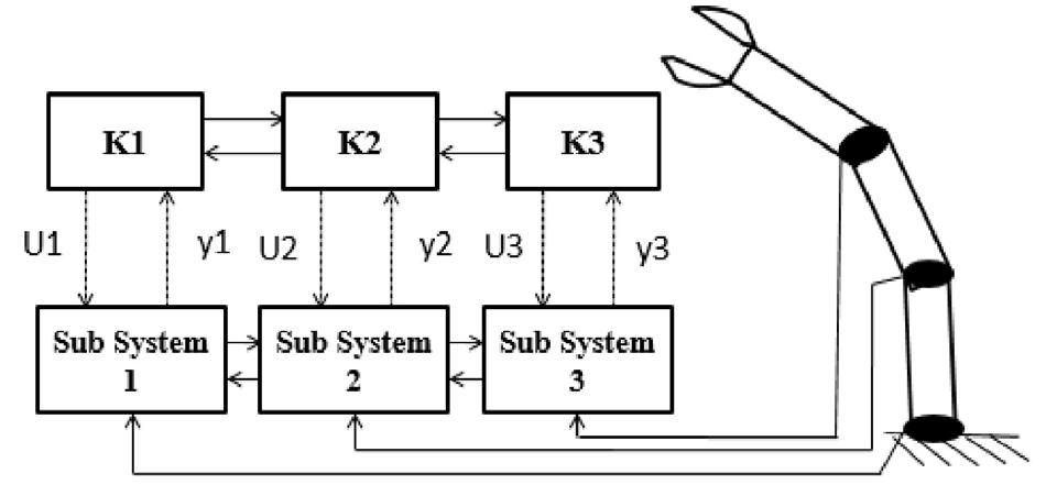
Fig. 4. Distributed manipulator control architecture

A simple distributed control scheme. The model-based control law given in Eqn. (2) represents a control law using the centralized control architecture, where a single central controller computes control inputs, τi, i=1,…,N, for all the joints. Note that here all the variables τ, θ, θ, θ , E, E , etc. are obtained in time t. Consider a simple distributed control law [17] for the ith joint level controller as:

Here, the index j (or i) is used to indicate the corresponding component of a vector, and Mij is the jth element in ith row of M. Note that the Eqn. (4) is the ith component of the model-based control law as given in Eqn. (2). Let Ki be the ith joint level controller using the control law given in the Eqn. (4). For the model-based control law given in here, we make following observations:

1. The output of each controller Ki is τi, the control input to the ith joint.

2. Controller Ki requires inputs from other jointlink agents which it may receive through the corresponding joint level controllers Kj, j ≠ i.

3. The controller Ki is connected to neighboring controllers Ki-1 and Ki+1, in the sense that it can send and receive signals.

4. Now the adjacency graph of Ki is connected.

5. Thus, the controller Ki can receive (send) signals from (to) any controller Kj, j ≠ i through a distributed (multi-hop, if required) communication.

6. The adjacency graph formed by the joint level controllers is identical to that formed by the jointlink agents.

Thus, the control architecture, where each joint level controller Ki controls the ith joint while obtaining necessary information (such as feedback values of joint states and the desired states), from the neighboring joint level controllers has a natural distributed architecture, which in fact is the result of the distributed nature of the manipulator dynamics. As observed in Remark 1, the joint level controllers are allowed to

communicate directly with the immediate neighbors, and as every joint level controller is indirectly connected to every other controller, the required information may be obtained through (multi-hop) distributed communication between the joint level controllers. Hence, though the control law corresponding to Ki may contain terms corresponding to every joint/link, not only those corresponding to the immediate neighboring agents, the control scheme based on the Eqn. (4) is naturally amenable for a distributed implementation.

Theorem 1. The control law given by the Eqn. (4), with positive gains, makes the links of the manipulator whose dynamics is given by the Eqn. (1), follow the desired trajectory θd(t), asymptotically.

Proof The closed-loop error dynamics may be obtained from Eqn (4) and Eqn. (1) as,

12,, , (5)

Thus, we have Ej → 0, as

for positive gains.

Remark 2. Here, the closed-loop error dynamics is identical to that obtained using the conventional model-based control scheme given by Eqn. (2). This is not surprising for two reasons. First, the joint level controllers Ki and the distributed control scheme presented here are based on the control laws given in Eqn. (4), which itself is based the control law given in Eqn. (2). Second, any control law that cancels the nonlinear and coupled dynamics using feedback, or in other words, achieves feedback linearization, should result in linear decoupled closed-loop error dynamics as given in Eqn. (5). The contributions here are: identifying a natural distributed nature of the model-based control law given in Eqn. (2), presenting a control scheme that is amenable for implementation in the distributed control architecture, and obtaining feedback linearization leading to guaranteed state independent trajectory tracking performance, unlike the decentralized (or independent joint) control schemes presented in the literature.

Remark 3. The distributed control scheme given by the Eqn. (4) is only a simple example of a control scheme/ law that can be implemented in the proposed distributed manipulator control architecture. In principle, several model-based control schemes may be designed within the proposed distributed architecture.

Distribution effectiveness. The main objective of the distributed control law for a manipulator being reduction in the cost of computation involved in the control law, we define a quantity known as distribution effectiveness. Let CTi be the computational cost associated with the ith joint level controller, and CTc be that associated with the corresponding centralized controller. Now we define the distribution effectiveness for N degree of freedom robot as

In an ideal situation, when the computation is distributed uniformly among the individual controllers, we get ηd = 1

5. Discrete-Time Implementation: Effect of Time

The model-based (centralized) control law as given in Eqn. (2) is in continuous time domain. However, in reality, this control law is realized in discrete time. The model-based control law in discrete time is given by τθ θ θ tM tT tT KE tT KE tT Ct T dd dV d Pd d () =−() () () +−() +−() +−() ( ,  θ θ tT Gt T d d () () +−() () (7)

Where, Td is the time delay introduced due to the sampling time Td. The sampling time depends on the time required to compute the control law Eqn. (7), along with any other processing required. Note that with the discrete control law given in Eqn. (7), feedback linearization is not achieved. We can achieve the feedback linearization only when Td = 0. However, due to the continuity of the dynamics of the manipulator and the model-based control law, tracking performance is expected to degrade gracefully with increasing Td. Now consider the discrete-time distributed control law based on that given in Eqn. (4),

Here, Tdd is the time delay (due to sampling time) in the discrete time distributed model-based control law. Note that it is expected that Tdd < Td as the computational effort associated with the control law is now shared among the individual controllers. Hence, it is expected that the trajectory tracking performance of manipulator with the discrete time distributed model-based control law (8) is superior to that with the centralized, discrete-time model-based control law given in Eqn. (7).

6. Distributed Control for a 3R Planar Manipulator

Now we shall illustrate the control scheme given by Eqn. (4) implemented in the proposed distributed control architecture using a simple 3R planar manipulator. We consider a 3R planar manipulator for several reasons. First, most manipulators use

revolute joints, which result in nonlinearities and dynamic coupling. Second, a serial-link planar manipulator has maximum dynamic coupling between its links. Third, it is a simplest (in terms of degrees of freedom) manipulator with at least one intermediate link, and fourth, it is a simplest (in terms of degrees-of-freedom) redundant manipulator (considering only tool position in a plane without considering its orientation).

Figure 5 shows the block diagram of the control law (Eqn. (4)) implemented in the proposed distributed architecture. The communication links, along with the information exchange between the neighboring controllers are also shown.

Fig. 5. Block diagram of the proposed model-based control of a 3R planar manipulator in the proposed distributed architecture

The ith joint level controller Ki receives the desired trajectory (θid;  θid ;  θid ) and the actual (or the current values of) (θi;  θi ;  θi ) in the form of sensory feedback, as inputs, and computes the control input τi as given by the control law (4), for the ith joint. Controllers communicate the values of corresponding joint variable (feedback) and desired joint variable (along with necessary derivatives not shown in the figure), that they received, to the immediate neighbors. The intermediate controller K2 communicates the values of θ1 (feedback it received via K1, along with its first and second derivatives) and θ1d (desired value it received via K1) to K3, and the values of θ3 (feedback it received via K3, along with the first and second derivatives) and θ3d (desired value it received via K3) to K1. Now with this distributed multi-hop communication between the individual joint level controllers, each of them has all the necessary information to compute the corresponding control law. Finally, the controller Ki provides the control input τi to the ith joint (the ith joint-link agent) using Eqn. (4) or (8).

Remark 4. The control scheme provided in Fig. 5 may be implemented in hardware. The joint level controllers may be implemented on an embedded hardware with a provision for necessary communication between them. In the case of distributed control of a manipulator, unlike in a typical multi-agent/robotic system, it is possible to use wired communication between the joint level controllers. However, a detailed

discussion on the hardware implementation is beyond the scope of this paper.

Computational cost and distribution effectiveness. Table 1 shows the number of addition (NA), multiplication (NM), along with the corresponding computational cost and the total computational cost (CT) of computing dynamics at each joint level. We obtain a distribution effectiveness of 0.66 in this case, as against an ideal value of 1. The maximal computational cost with the distributed implementation now reduces from 944 units to 480 units, that is about 50% of the cost of centralized implementation. This implies that the sampling time of a discretized implementation of the control law in the distributed architecture is about half that of the centralized architecture. If the computational load were distributed equally among the joint level controllers, then the computational cost, and hence the sampling time, with the distributed implementation would have been 33% of that with the centralized implementation. Thus, though the model-based control law implemented in both centralized architecture (Eqn. (2)) and the proposed distributed architecture Eqn. (4) are theoretically identical, in reality, when the control law is implemented in discrete time, the trajectory tracking performance with the control law in distributed architecture is expected to be superior compared to that with the centralized architecture as Tdd = 0.5 T d. If we carefully design the distributed control law such that ηd = 1, then we obtain Tdd = 0. 33 T d, the least possible sampling time. As shown in Table 2, the distribution effectiveness θ d improves with degrees-of-freedom of the manipulator. It may be observed that manipulator control in the distributed architecture is more useful for the higher degrees-of-freedom manipulator due to higher computational cost of the centralized control law and better distribution effectiveness.

Tab. 1. Number of additions (NA), multiplications (NM), corresponding costs (CA;CM), and the total cost (CT), involved in computation of the dynamics at each joint

Tab. 2. Distribution effectiveness with the degrees-offreedom of planar manipulators

Remark 5. We may observe that the distributed control scheme based on Eqn. (4) presented here is based on the identification of a natural distributed nature of the manipulator dynamics itself and that of the model-based control law (2). The reduction in computational lead-time with the distributed control scheme is achieved purely because of the distribution of the computational effort among the joint level controllers, rather than the program optimization or operation optimization techniques that are used at the algorithmic level.

Tab. 3. Terms appearing multiple times in 3R manipulator dynamic equation

joint level is now reduced by about 60% compared to that shown in Table 1. However, the distribution effectiveness ηd = 0:66 even in this case, indicating that this exercise of reducing computations by avoiding repeated computation of certain repetitive terms does not affect how the computation load is shared among the individual controllers.

Remark 6. Apart from the reduction in computational overhead due to the natural distribution of the computational effort among the joint level controllers, we have achieved further reduction in the computational load here by identifying repetitive terms in the manipulator dynamics/control law. As demonstrated by the fact that the distribution effectiveness is unaffected by this exercise, this process of reduction in computational load is independent of the distributed property of the manipulator dynamics or the proposed distributed control scheme.

7. Results and Discussion

5

Reducing computational cost. With careful observation, we can identify several repetitive terms in the dynamics of a 3R planar manipulator. Such repetitive terms are shown in Table 3 along with the number of repetitions. For example, the term () −+ls g 1 1 2 1 θ repeats ten times in the equation corresponding to the first joint, seven times in that corresponding to the second joint, and twice in that corresponding to the third joint.

Tab. 4. Number of addition and multiplication, corresponding computational cost after avoiding repetitive computation of terms shown in Table 3

Now if we compute each of the terms that are listed in Table 3 only once, we may further reduce the computation cost associated with dynamics, and hence, that of the control law, at each joint. Note that this reduction is achieved without neglecting any of the terms. Table 4 shows the number of addition, multiplication, along with the corresponding computational cost and total computational cost of computing dynamics at each joint level after this refinement. It may be observed that the computational cost at each

In this section, we present results of simulation experiments carried out in Matlab to illustrate and compare the trajectory tracking performance of the proposed control scheme with a simple decentralized PID control scheme. We also provide a discussion on the comparison of the proposed control scheme with that of the decentralized control schemes in general.

Simulation results. First, we present the results of simulation experiments. We have simulated the proposed distributed control scheme for a 3R planar manipulator using Matlab/Simulink. We considered a manipulator with m1 = 10kg, m2 = 10kg, and m3 = 10kg, and l1 = 5m; l2 = 6m, and l3 = 5m. We considered a sinusoidal trajectory as the desired trajectory to be followed by each of the joints.

Figures 6(a)-(c) show the trajectory tracking performance of the first, second, and third joints of the manipulator with the decentralized PID controller. Figures 7(a)-(c) show the trajectory tracking performance of the first, second, and third joints of the manipulator with the proposed distributed control. It can be observed that all the joints successfully track the respective desired trajectories with the proposed distributed controller. Though the performance with the decentralized PID control may be improved by tuning the controller gains, as observed earlier, due to the nonlinear nature of the manipulator dynamics, the performance level cannot be guaranteed to be uniform across the state-space. As expected, it was observed during the simulation experiments that the trajectories obtained with the proposed distributed control scheme were identical to that obtained with the centralized model-based control scheme.

Distributed vs decentralized schemes. Now we provide an informal discussion comparing the proposed distributed (or centralized) control scheme with the

Fig. 6. Trajectory tracking performance of a) first, b) second joint, and c) third joint, of a 3R planar manipulator with independent joint PID controller

decentralized control scheme in general. The independent joint PID controller is probably the simplest control scheme reported in the literature in the decentralized control architecture. Each of such schemes leads to different trajectory tracking performance, which is expected to be better than that with the independentjoint PID control scheme. However, when the system model is fully available, it has been established theoretically that the trajectory tracking performance with the model-based nonlinear control is superior to that with any other control scheme which does not consider the model fully, particularly the coupled dynamics. In the case of control schemes in decentralized architecture inspite of using adaptive control or other techniques to account for unmodelled dynamics, there is no provision for accounting for the coupling dynamics between the links. Apart from this theoretically established fact of resulting in an inferior trajectory tracking perfor-

mance compared to that with the model-based control (centralized or distributed), the decentralized control schemes proposed in the literature (unlike the simple independent joint PID scheme) may not be computationally very inexpensive.

Thus, we may observe that though the decentralized schemes reported in the literature may have marginally lower computational overhead as compared to the proposed model-based control in the distributed architecture, their trajectory performance is expected to be inferior, at least in a theoretical sense and ideal situations, to that with the distributed scheme proposed in this work.

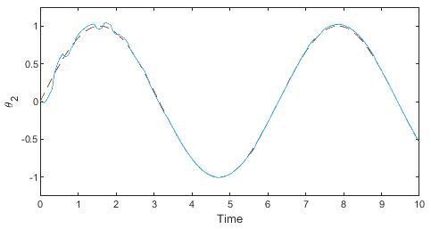
Fig. 7. Trajectory tracking performance of a) first, b) second joint, and c) third joint, of a 3R planar manipulator with the proposed control scheme

Though we consider the manipulator dynamics is known completely in this work, it may not be the case in reality. When the model is not known exactly, it is possible to use techniques such as adaptive control within the distributed control architecture. However, the focus of this paper is on control schemes implemented in a distributed architecture and establishing equivalence of the centralized and distributed architecture.

(c)

(a)

(b)

(c)

8. Conclusion

We proposed a distributed model-based control architecture for a manipulator. The classical model-based control law was used to demonstrate the proposed architecture by implementing it in a distributed manner. The distributed control scheme provided was shown to lead to a stable, linear, decoupled, second order error dynamics. The trajectory tracking performance with the proposed distributed model-based control scheme was observed to be identical to that with the centralized model-based control under ideal conditions. Further, with the proposed control scheme, the computational lead-time is shown to reduce considerably by distributing the computational effort among the individual controllers. This reduction in computational lead-time in turn was observed to improve the tracking performance when the control law is realized in discrete time. In contrast to the decentralized or independent-joint control schemes reported in the literature, the coupling dynamics are not neglected in the proposed distributed control scheme. Simulation results using Matlab were provided to demonstrate that the tracking performance of a 3R planar manipulator with the proposed distributed model based control scheme is superior to that with the decentralized PID control scheme.

A detailed comparison of the proposed distributed model-based control scheme with the decentralized control schemes presented in the literature in terms of the tracking performance and the computational time will be very useful. Some of the other directions for future work include design of distributed controller schemes to achieve a better distribution of the computational load, thereby improving the distribution effectiveness, and hence, reducing the computation lead time, devising a formal methodology for the design of the distributed control for a general serial link robot, experimental verification of the control scheme, etc.

AUTHORS

S. Soumya* – Instrumentation and Control Engineering, Manipal Institute of Technology, Manipal, Karnataka, India, e-mail: soumya5.subbu@gmail.com.

K. R. Guruprasad – Department of Mechanical Engineering, National Institute of Technology Karnataka, Surathkal, India.

*Corresponding author

R EFERE n CES

[1] F. Aghili, “Torque control of electric motors without using torque sensor”. In: 2007 IEEE/RSJ International Conference on Intelligent Robots and Systems, 2007, 3604–3609, DOI: 10.1109/IROS.2007.4399145.

[2] P. Bohner and R. Luppen, “Reactive multi-agent based control of redundant manipulators”. In: Proceedings of International Conference on Robotics and Automation, vol. 2, 1997, 1067–1072, DOI: 10.1109/ROBOT.1997.614276.

[3] S.-J. Cho, J. S. Lee, J. Kim, T.-Y. Kuc, P.-H. Chang and M. Jin, “Adaptive time-delay control with a supervising switching technique for robot manipulators”, Transactions of the Institute of Measurement and Control, vol. 39, no. 9, 2017, 1374–1382, DOI: 10.1177/0142331216637118.

[4] P. Dasgupta, J. Baca, K. R. Guruprasad, A. MuñozMeléndez and J. Jumadinova, “The COMRADE System for Multirobot Autonomous Landmine Detection in Postconflict Regions”, Journal of Robotics, vol. 2015, 2015, 1–17, DOI: 10.1155/2015/921370.

[5] K. R. Guruprasad, Robotics: Mechanics and Control, PHI LEARNING, 2019.

[6] K. R. Guruprasad and A. Ghosal, “Model Reference Learning Control for Rigid Robots”. In: Proceedings of the ASME Design Engineering Technical Conferences, 1999, 1-9.

[7] K. R. Guruprasad and D. Ghose, “Automated Multi-Agent Search Using Centroidal Voronoi Configuration”, IEEE Transactions on Automation Science and Engineering, vol. 8, no. 2, 2011, 420–423, DOI: 10.1109/TASE.2010.2072920.

[8] “Complete Coverage of an Initially Unknown Environment by Multiple Robots using Voronoi Partition”. K. R. Guruprasad, Z. Wilson and P. Dasgupta, https://pdfs.semanticscholar. org/2981/639efaf2931e24b1d0be8fd8cba6aeb18e35.pdf. Accessed on: 2020-05-28.

[9] M. Hashimoto, “Robot motion control based on joint torque sensing”. In: 1989 International Conference on Robotics and Automation Proceedings, 1989, 256–261, DOI: 10.1109/ROBOT.1989.99998.

[10] T. C. Hsia and L. S. Gao, “Robot manipulator control using decentralized linear time-invariant time-delayed joint controllers”. In: Proceedings of IEEE International Conference on Robotics and Automation, 1990, 2070–2075, DOI: 10.1109/ROBOT.1990.126310.

[11] S.-H. Hsu and L.-C. Fu, “A fully adaptive decentralized control of robot manipulators”, Automatica, vol. 42, no. 10, 2006, 1761–1767, DOI: 10.1016/j.automatica.2006.05.012.

[12] H. Jia, W. Zhuang, Y. Bai, P. Fan and Q. Huang, “The Distributed Control System Of a Light Space Manipulator”. In: 2007 International Conference on Mechatronics and Automation, 2007, 3525–3530, DOI: 10.1109/ICMA.2007.4304131.

[13] L. Jin, S. Li, J. Yu and J. He, “Robot manipulator control using neural networks: A survey”, Neurocomputing, vol. 285, 2018, 23–34, DOI: 10.1016/j.neucom.2018.01.002.

[14] K. Kosuge, H. Takeuchi and K. Furuta, “Motion control of a robot arm using joint torque sensors”, IEEE Transactions on Robotics and Automation, vol. 6, no. 2, 1990, 258–263, DOI: 10.1109/70.54743.

[15] S. Li, H. Wang and M. U. Rafique, “A Novel Recurrent Neural Network for Manipulator Control With Improved Noise Tolerance”, IEEE Transactions on Neural Networks and Learning Systems, vol. 29, no. 5, 2018, 1908–1918, DOI: 10.1109/TNNLS.2017.2672989.

[16] M. Liu, “Decentralized PD and Robust Nonlinear Control for Robot Manipulators”, Journal of Intelligent and Robotic Systems, vol. 20, no. 2, 1997, 319–332, DOI: 10.1023/A:1007968513506.

[17] M. Liu, “Decentralized control of robot manipulators: nonlinear and adaptive approaches”, IEEE Transactions on Automatic Control, vol. 44, no. 2, 1999, 357–363, DOI: 10.1109/9.746266.

[18] A. Mori, F. Naya, N. Osato and T. Kawaoka, “Multiagent-based distributed manipulator control”. In: 1996 IEEE/SICE/RSJ International Conference on Multisensor Fusion and Integration for Intelligent Systems, 1996, 289–296, DOI: 10.1109/MFI.1996.572190.

[19] P. Poignet and M. Gautier, “Nonlinear model predictive control of a robot manipulator”. In: Proceedings of 6th International Workshop on Advanced Motion Control, 2000, 401–406, DOI: 10.1109/AMC.2000.862901.

[20] L. E. Pfeffer, O. Khatib and J. Hake, “Joint torque sensory feedback in the control of a PUMA manipulator”, IEEE Transactions on Robotics and Automation, vol. 5, no. 4, 1989, 418–425, DOI: 10.1109/70.88056.

[21] H. Seraji, “Decentralized adaptive control of manipulators: theory, simulation, and experimentation”, IEEE Transactions on Robotics and Automation, vol. 5, no. 2, 1989, 183–201, DOI: 10.1109/70.88039.

[22] J.-E. Slotine and L. Weiping, “Adaptive manipulator control: A case study”, IEEE Transactions on Automatic Control, vol. 33, no. 11, 1988, 995–1003, DOI: 10.1109/9.14411.

[23] S. Soumya and K. R. Guruprasad, “Model-based distributed cooperative control of a robotic manipulator”. In: 2015 IEEE International WIE Conference on Electrical and Computer Engineering (WIECON-ECE), 2015, 313–316, DOI: 10.1109/WIECON-ECE.2015.7443926.

[24] M. W. Spong and M. Vidyasagar, Robot dynamics and control, Wiley, 1989.

[25] T. Tsuji, S. Nakayama and K. Ito, “Distributed feedback control for redundant manipulators based on virtual arms”. In: Proceedings ISAD 93: International Symposium on Autonomous Decentralized Systems, 1993, 143–149, DOI: 10.1109/ISADS.1993.262710.

[26] Z.-J. Yang, Y. Fukushima and P. Qin, “Decentralized Adaptive Robust Control of Robot Manipulators Using Disturbance Observers”, IEEE Transactions on Control Systems Technology, vol. 20, no. 5, 2012, 1357–1365, DOI: 10.1109/TCST.2011.2164076.

[27] J. Yim and J. H. Park, “Nonlinear H∞ control of robotic manipulator”. In: Proceedings of the IEEE International Conference on Systems, Man and Cybernetics, vol. 2, 1999, 866–871.

[28] J. S. Yuan, “Closed-loop manipulator control using quaternion feedback”, IEEE Journal on Robotics and Automation, vol. 4, no. 4, 1988, 434–440, DOI: 10.1109/56.809.

Path Planning Optimization and Object Placement Through Visual Servoing Technique for Robotics Application

Submitted: 19th March 2019; accepted: 20th November 2019

Sumitkumar Patel, Dippal Israni, Parth Shah

DOI: 10.14313/JAMRIS/1-2020/5

Abstract: Visual servoing define a new methodology for vision based control in robotics. Vision based action involve number of actions that move a robot in response of results of camera analysis. This process is important to operate and help robot to achieve a specific goal. The main purpose of visual servoing consists of considering a vision system by specific sensor dedicated to involve control servo loop and task. In this article, three visual control scheme: Image Based Visual Servoing (IBVS), Position Based Visual Servoing (PBVS) and Hybrid Based Visual Servoing (HBVS) are illustrated. The different terminologies are represented through effective workflow of robot vision. IBVS method concentrate on the image features that are immediately available in the image. This experiment is performed by estimating distance between camera and object. PBVS consist of moving object 3-D parameters to estimate measurement. This paper showcases PBVS using kuka robot model. HBVS uses the 2D and 3D servoing by combining visual sensors also it overcomes challenges of previous two methods. This paper represents HBVS method using IPR communication robot model

Keywords: Visual servoing, features, coordinates, kinematics, disparity, optimization, motion estimation

1. Introduction

In recent years, the advances on robotics research have been very effective. Many original problems have been either completely or at least partially solved. Visual servoing refer to use computer vision data to handle control motion of robots [1][2]. Vision data can be to collect from a camera that is mounted on robot manipulator. Another camera can be fixed in the work area so that observe the robot motion. The goal of robot is to react and reach targeted position using the visual data.

The pilot vision of the robot is defined as a “Visual servoing” [3]. The visual servoing is categorized into three different parts. (i) key element-based error function, (ii) the number of camera and their position (eyein-hand vs. eye-to hand configuration) and (iii) servoing structure though kinematic calculation. Servoing

structure is based on classical Image-Based Visual Servoing (IBVS) and Position Based Visual Servoing (PBVS) [2]. IBVS and PBVS are 2D and 3D approach respectively. IBVS is based on the specific set of images that focuses on the main image and it’s features. IBVS does not need any pose assessment or any other 3D approaches. It uses the features of the capture object. PBVS is a 3D approach that analyses the position of the robot according to the target object. PBVS uses the digital camera as a key-point to retrieve visual features [4]. It requires robust calibrations and 3D model to reach target position. In the hybrid system, it uses one single camera in hand and configuration of another stationary camera to observe the present object [5]. Hybrid model focuses on positional vision approach to minimize inappropriate result. This paper gives an overview of both IBVS and PBVS approach.

2. Related Work

Till now many visual servoing based algorithm and techniques are implemented. Some of the algorithms and techniques are discussed below:

Gans et al. introduced technique to switch over between IBVS and PBVS [6]. In the case of lower visibility IBVS techniques is applied. However, in complex situation the proposed hybrid switching system again redirects to PBVS. This suggested technique stops the system failure and provide asymptotic stability in IBVS and PBVS.

G. Flandin et al. proposed an idea using eye-tohand camera. They have used kalman filter [6] to perform positioning at goal area with efficiency. They applied tracking techniques in local image to make sure position in global image.

Denavit et. al suggested a technique that require four parameters to estimate join of two robots. They use kinematics estimation to make a rotation and other transformation of robot joins. The estimation of kinematics can be classified into two categories: (i) forward kinematics and (ii) inverse kinematics.

Fedrizzi et al. introduce ARPlace (Action-related place). The goal is to point on specific position using AR Place. Further, they use probability of position to calculate next position of target object. The probability of visualization representation based on low to high color intensity [7].

Corke et al. presented closed loop positon control system that gives high performance in providing robot positioning commands at high rates. In this system image processing subsection comprised completely of off-the-shelf components. It enables system to identify the target object either or not relative motion between object and camera [8].

3. Control Based Vision

Visual servoing is classified into two different types. Such as (i) camera configuration and (ii) structure servoing. Robot arm motion has several challenges like the camera lens configuration, position estimation, feature extraction, image and video controlling. This issue needs visual servoing to solve the problem. Basic camera configurations. A camera is used to perform operation by projecting 3D points to the plane of the image. Image cell is more sensitive for the measurement. A camera measures level of intensity, the light etc.

It uses coordinate C = (M, N, O,1) with respect to A = ( X, Y,1). A ∝ { P 0 }C (1) where P = fACfAc C fAd D cotcot sins in ∅ ∅ () ()

where Co and Do are pixel coordinate for the point Ac and Ad, respectively f is the main length and also Ac = Ad.

Visual area is categorized in two types such as “Eye-to-hand” and “Eye-in-hand”. In Eye-to-hand eye is mounted on the robot arm and not allowed to pose any kind of motion. This categories whole workspace cannot be visualized. Hence, this category limits the number of objectives to be achieved. This vision is called an Eye-in-hand [8]. In Eye-to-hand category, the arm can also be visualized the mounted camera in such a way that it can control workspace coordinates with arm movement. Eye-to-hand works on the top of the object and other desired location [9].

IBVS focuses on coordinates of the object and control the robot vision. The captured image features compare with the desired image position to control and specify robot grasp movement [10]. In Control servoing time picture is captured by using camera that focuses on desired features and eliminates error by comparing both images. Such process is useful to decide workspace for robot.

The primary goal of IBVS is to target desire object and eliminate movement according to specified input and references of image [11].

The approximation of accuracy, stability and per-formability depend on the camera and target point. The estimation of accuracy and stability is challenging but using the visual features [12], polar, spherical coordinate [13], special movement features and cylindrical it can be estimated.

The Fig. 4 represents the extrinsic parameters [14] for visualization and two camera use for the servoing. These two cameras results are relatively compared.

From Fig. 4 number (1) and (2) represent the camera uses to estimate extrinsic parameter of the vision respectively.

3.1. Image Based Visual Servoing / 2D Servoing

All scenarios are based on the each and every frame of the camera video file also it computes based on the stereo camera calibration and triangulation method [15] to estimate the focus point.

Fig. 2. Image-based visual servoing

Fig. 3. Extrinsic parameters visualization

Fig. 1. Structure of visual servoing

Reading and rectifying the video frames. The video file reader is used to read camera video frame and display the video file. Rectifying field compute the disparity [16] based on the matching with left camera vision to right camera vision and generate the 3-D plane [17].

Disparity Estimation. The disparity of rectified image corresponding point locates to the same pixel of the row. Corresponding distance is measured pixel of left with pixels of right. This distance called disparity [16] which proportional to the distance between camera points.

3-D Reconstruction. 3D coordinate points are used from the disparity map which generated by left and right camera red-cyan glasses. It converts directly to the meters and generate the cloud streaming point. The cloud point visualizes vertical axis and is directed by the streaming point [18].

Detect the people and Distance measurement. It detects the people with the use of system object focus point. The detected people’s distance measure using the centroid point taken from the 3D coordinate. It calculated results using the two camera and detected people.

D = sqrt(sum(centroid of 3D * ^ 2) (2)

where D respect to distance between the camera and generated centroid point.

Write video and analyses the rest of the video file. Until so far used 3-D coordinate process, detect the people and generate meters for measurement in specific frame of the video data. For every frame it processes same as previous, read, rectifies and converts into grayscale, computation of the disparity, generation of the 3-D cloud point. Hence, those process to detect the people by using centroid of people. This Centroid point helps to find the distance in the meter.

3.2. Position Based Visual Servoing

PBVS method focuses on the 3D information of the object. In this method, object coordinates captured are in 2D there by it converts into 3D graph and tracks the object [19] [20].

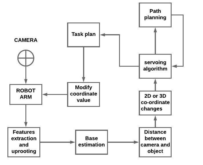
Fig. 4. Position based visual servoing

The diagram process shows the process of robot movement to grasp the object.

In PBVS number of algorithms and kinematics inverse operations are used for path planning. kinematic operations [21] focuses on the forward and inverse operation [22]. Robot movement handles various path and focuses on the current and desire position.

Features extraction. Features are the key-point for servoing. It extracts and matches the current features [23]. The qualities of feature are not always dependent on the type of features, extracted results and image techniques but it also the vision of the robot system. Features are easy to identify and can be measured with higher accuracy.

The distance between camera and object. The main objective of this process is to estimate motion and trajectory based tracking to approximate the object. This process is performed by path finding and route optimization algorithm [24].

2D or 3D coordinates changes. Object detection and position approximation while sometime captures unclear position is captured. This results are challenge for generation of 3D coordinate to solve the mention problem. The position is estimated by separately converting 2D image into 3D.

Servoing algorithm and path planning. Robot path selection is performed using the number of different algorithm such as ant colony optimization [25] [26], cyclic coordinate descent [27] [28], particle swarm optimization [29] [30]. Algorithm results generate number of possible solution is selected among them the shortest path without obstacle.

Task plan. Task plan process is executed after algorithm results and those result is directly applied to make robot to reach at the target position. However, at servoing time there can be circumstances that obstacle may be present in the route of the workspace. In that scenario, it again analyzes the obstacle avoidance algorithm [31] and again generates best path to reach the target.

Model-based visual servoing. This approach uses to project the coordinate from initial position to targeted workspace. Model based visual servoing is computed based on the knowledge of the 3D coordinate.

The control strategies are used for driving the robot using single camera. It uses the Visual Servoing Platform libraries (ViSP)

Overall, in PBVS the sensitivity and calibration of the camera is required to reduce the error during the control.

3.3. Hybrid Based Visual Servoing

The two previous method IBVS and PBVS plays important role in HBVS to handle the position of the robot. HBVS method of servoing is mainly used the 2 ½ D servoing [32] and movement Partition based [33].

HBVS suitably combines unique benefits of both IBVS and PBVS. The tracking system combines inputs from the camera and sensors to estimate the moving target position. Color segmentation to finds the target image region with the associated moving target object.

HBVS overcomes disadvantage of IBVS and PBVS. It does not require the fully completed 3D model for the object analysis [34]. HBVS method reduces the rotation for all robot DOFS. This pure rotation is based on the optical axis and combines or switching in between the IBVS and PBVS when it necessary.

The stereo image vision taken by the gripper model which compare with the original images. It generates 3D coordinates point and measure distance by stereo image [35]. The number of filters are applied to matches the result for minimizing the drawback and error. Due to that reason it used combination of two camera result (eye-in-hand and eye-to-hand) [36] [37].

On the other method, re-projection method may minimize error though using the numerical solution of camera projection. It uses the number of projection point instead of stereo images. The number of camera to generate frame for different measurement method and select path related to object [35].

4. Qualitative Analysis Through Real-Time Application

The experiment is conducted for three different methods such IBVS, PBVS and HBVS for the qualitative assessment. These three experiment are implemented using different robot models.

4.1.

Image Based Visual Servoing / 2D Servoing

In IBVS the algorithm and other flow of the result analysis is measured by calculating the distance between camera and object.

As show cases in fig. 6 the image taken from the video frame is captured by the camera. The specific frame is rectified by red – cyan glass. The rectified image combines the anaglyph graph. It interprets the 3D effect and rectified image based on horizontal epipolar line. From fig. 7 lts aligned into row direction. Finally, the disparity of rectified stereo images are calculated.

The method generates 3D cloud point according to the disparity of rectified frames. According to the 3D cloud point it takes centroid and detect the people and measure the distance as shown in fig. 9.

4.2.

Position Based Visual Servoing

PBVS estimate the calibration, pose parameters and the matrix computation to make an accurate and stable to result. PBVS analyses result quite positive in comparison with IBVS. PBVS extract information from the vision sensor and handle robot motion.

The example of PBVS is represented that is implemented on webot robot simulator with kuka model [38] and matlab. Webot simulator and kuka model helps to move object from initial location to target

Fig. 5. Hybrid visual servoing

Fig. 6. The image taken from the camera and rectified by red-cyan glass

Fig. 7. Generated disparity map according to rectified frame

location with the help to robot DOFS and grippers. Gripper helps to grab the object by detecting the position and object place of another workspace area [38] [39].

location

In Fig. 10 at the initial stage the robot identifies the pose of object. The mounted camera in gripper detects the cube and holds object placed on the box. As seen in fig. 11 the held object is placed to the plate of the robot and object is moved to another location from the box. According to the fig. 13 reaching at target location robot DOFS again picks and places object from the plate to destination.

4.3. Hybrid Based Visual Servoing

In HBVS method robot model exchanges the object by IPR robot and it carry the object from one bucket and places into other bucket. For exchanging robot communication uses the color code communication using 3D model and the kinematic operations. In Kin-

Fig. 10. Detecting the object

Fig. 11. Catching through gripper

Fig. 12. An object placed on the plate

Fig. 13. The object moved to another

from the box

Fig. 8. 3-D coordinate point and cloud point

Fig. 9. Detected person and distance from the camera using meter as a unit

ematic operations the inverse operation, forward operation and Jacobean matrix operation [40][41]. Although all the communication of HBVS are used through either Eye-in hand or Eye-to hand process. Two IPR robot model are placed for exchanging the object with the help of webot simulator. The different languages such C, C++, Matlab and Python are used for the core purpose.

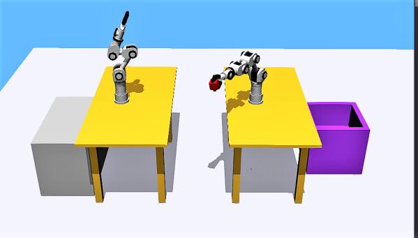
The two IPR model position are shown in Fig. 15 to take object from initial location through gripper. The model contact with each other and shares the object

as in fig14. The shared object to reach at target location by their path through multipoint mediator [42]. The given results from fig. 15 after reaching at target location robot un-holds the gripper and drops the red cube inside the box.

These simulation results represent object communication with IPR communication robots. Servoing camera helps to capture initial location of object and analyses the presence of object at given = location. Robot gripper holds the object and uses the optimal route via the kinematic operation and path optimization algorithm. There are several path optimization algorithms such as particle swarm optimization, ant colony optimization, cyclic coordinate decent, etc. It generates shortest path for servoing system which provides better time complexity and faster operation.

This work can be further enhanced by integrating object tracking techniques with visual servoing to improve the performance as well as accuracy [43] [44] [45].

5. Conclusion

Visual servoing is a technique which is used for controlling autonomous dynamic system. A number of application from object grasping to mobile robot navigation is now possible. This paper consists different techniques such as IBVS, PBVS and HBVS. IBVS model in which image based distance measuring of the object is being done using two cameras stereo vision. In PBVS method object pick and place operation perform using the kuka robot model. Another, the experimental results of HBVS is used to solve and improve image-based and position-based visual servoing and IPR collaboration robot model used for exchanging object from initial location to target location. In future this can be extended for resolving calibration error, path planning, obstacle avoidance, estimating shortest path.

A CK n OW le D gemen TS

The authors would like to thank CHARUSAT Space Research and Technology Center (CSRTC) for providing required resources to carry out research work.

AUTHORS

Sumitkumar Patel – U and P U. Patel Department of Computer Engineering, Chandubhai S. Patel Institute of Technology (CSPIT), Charotar University of Science and Technology (CHARUSAT), Gujarat, India, e-mail: sumitpatel47@gmail.com.

Dippal Israni* – Information Technology Department, R. C. Technical Institute, Ahmedabad, India, e-mail: dippalisrani90@gmail.com.

Parth Shah – Department of Information Technology, Chandubhai S. Patel Institute of Technology (CSPIT), Charotar University of Science and Technology

Fig. 14. Position of two IPR models

Fig. 15. Object exchange by IPR robot

Fig. 16. Object shared by IPR robot

Fig. 17. Object placed at destination location

(CHARUSAT), Gujarat, India, e-mail: parthshah.ce@ charusat.ac.in.

* Corresponding author

Re F e R en C e S

[1] P. K. Allen, B. Yoshimi and A. Timcenko, “Realtime visual servoing”. In: Proceedings. 1991 IEEE International Conference on Robotics and Automation, 1991, 851–856, DOI: 10.1109/ROBOT.1991.131694.

[2] B. Thuilot, P. Martinet, L. Cordesses and J. Gallice, “Position based visual servoing: keeping the object in the field of vision”. In: Proceedings 2002 IEEE International Conference on Robotics and Automation, vol. 2, 2002, 1624–1629, DOI: 10.1109/ROBOT.2002.1014775.

[3] A. C. Sanderson and L. E. Weiss, “Image-based visual servo control using relational graph error signals”. In: Proc. IEEE Conference on Cybernetics and Society, 1980.

[4] F. Chaumette and S. Hutchinson, “Visual servo control. II. Advanced approaches”, IEEE Robotics & Automation Magazine, vol. 14, no. 1, 2007, 109–118, DOI: 10.1109/MRA.2007.339609.

[5] J. T. Feddema, C. S. G. Lee and O. R. Mitchell, “Weighted selection of image features for resolved rate visual feedback control”, IEEE Transactions on Robotics and Automation, vol. 7, no. 1, 1991, 31–47, DOI: 10.1109/70.68068.

[6] N. R. Gans and S. A. Hutchinson, “An asymptotically stable switched system visual controller for eye in hand robots”. In: Proceedings 2003 IEEE/RSJ International Conference on Intelligent Robots and Systems (IROS 2003), vol. 1, 2003, 735–742, DOI: 10.1109/IROS.2003.1250717.

[7] A. Fedrizzi, L. Mosenlechner, F. Stulp and M. Beetz, “Transformational planning for mobile manipulation based on action-related places”. In: 2009 International Conference on Advanced Robotics, 2009, 1–8.

[8] P. I. Corke and R. P. Paul, “Video-rate visual servoing for robots”. In: V. Hayward and O. Khatib (eds.), Experimental Robotics I, vol. 139, 1990, 429–451, DOI: 10.1007/BFb0042533.

[9] G. Flandin, F. Chaumette and E. Marchand, “Eye-in-hand/eye-to-hand cooperation for visual servoing”. In: Proceedings 2000 ICRA. Millennium Conference. IEEE International Conference on Robotics and Automation. Symposia Proceedings, vol. 3, 2000, 2741–2746, DOI: 10.1109/ROBOT.2000.846442.

[10] P. Ardón, M. Dragone and M. S. Erden, “Reaching and Grasping of Objects by Humanoid Robots Through Visual Servoing”. In: D. Prattichizzo, H. Shinoda, H. Z. Tan, E. Ruffaldi and

A. Frisoli (eds.), Haptics: Science, Technology, and Applications, vol. 10894, 2018, 353–365, DOI: 10.1007/978-3-319-93399-3_31.

[11] A. McFadyen, M. Jabeur and P. Corke, “ImageBased Visual Servoing With Unknown Point Feature Correspondence”, IEEE Robotics and Automation Letters, vol. 2, no. 2, 2017, 601–607, DOI: 10.1109/LRA.2016.2645886.

[12] F. Chaumette, “Image Moments: A General and Useful Set of Features for Visual Servoing”, IEEE Transactions on Robotics, vol. 20, no. 4, 2004, 713–723, DOI: 10.1109/TRO.2004.829463.

[13] R. T. Fomena and F. Chaumette, “Improvements on Visual Servoing From Spherical Targets Using a Spherical Projection Model”, IEEE Transactions on Robotics, vol. 25, no. 4, 2009, 874–886, DOI: 10.1109/TRO.2009.2022425.

[14] S. Miyata, H. Saito, K. Takahashi, D. Mikami, M. Isogawa and A. Kojima, “Extrinsic Camera Calibration Without Visible Corresponding Points Using Omnidirectional Cameras”, IEEE Transactions on Circuits and Systems for Video Technology, vol. 28, no. 9, 2018, 2210–2219, DOI: 10.1109/TCSVT.2017.2731792.

[15] J. You, Y. Park, and H. Yoon, “United States Patent: 9781318 - Camera for measuring depth image and method of measuring depth image using the same, ” October, 2017.

[16] D. Kragic and H. I. Christensen, “Cue integration for visual servoing”, IEEE Transactions on Robotics and Automation, vol. 17, no. 1, 2001, 18–27, DOI: 10.1109/70.917079.

[17] Y. Ri and H. Fujimoto, “Image Based Visual Servo Application on Video Tracking with Monocular Camera Based on Phase Correlation Method”. In: IEEJ International Workshop on Sensing, Actuation, Motion Control, and Optimization, 2017.

[18] G. Chesi and A. Vicino, “Visual Servoing for Large Camera Displacements”, IEEE Transactions on Robotics, vol. 20, no. 4, 2004, 724–735, DOI: 10.1109/TRO.2004.829465.

[19] Y. Benbelkacem and R. Mohd-Mokhtar, “Position-based visual servoing through Cartesian path-planning for a grasping task”. In: 2012 IEEE International Conference on Control System, Computing and Engineering, 2012, 410–415, DOI: 10.1109/ICCSCE.2012.6487180.

[20] M. Keshmiri and W. F. Xie, “Catching moving objects using a Navigation Guidance technique in a robotic Visual Servoing system”. In: 2013 American Control Conference, 2013, 6302–6307, DOI: 10.1109/ACC.2013.6580826.

[21] P. Borrel and A. Liégeois, “A study of multiple manipulator inverse kinematic solutions with

applications to trajectory planning and workspace determination”. In: Proceedings. 1986 IEEE International Conference on Robotics and Automation, vol. 3, 1986, 1180–1185, DOI: 10.1109/ROBOT.1986.1087554.

[22] E. Hoffman, A. Rocchi, N. G. Tsagarakis and D. G. Caldwell, “Robot Dynamics Constraint for Inverse Kinematics”. In: J. Lenarčič and J.-P. Merlet (eds.), Advances in Robot Kinematics 2016, vol. 4, 2018, 275–283, DOI: 10.1007/978-3-319-56802-7_29.

[23] H. Wang, B. Yang, J. Wang, X. Liang, W. Chen and Y.-H. Liu, “Adaptive Visual Servoing of Contour Features”, IEEE/ASME Transactions on Mechatronics, vol. 23, no. 2, 2018, 811–822, DOI: 10.1109/TMECH.2018.2794377.

[24] M. Keshmiri and W.-F. Xie, “Image-Based Visual Servoing Using an Optimized Trajectory Planning Technique”, IEEE/ASME Transactions on Mechatronics, vol. 22, no. 1, 2017, 359–370, DOI: 10.1109/TMECH.2016.2602325.

[25] Q. Yang, W.-N. Chen, Z. Yu, T. Gu, Y. Li, H. Zhang and J. Zhang, “Adaptive Multimodal Continuous Ant Colony Optimization”, IEEE Transactions on Evolutionary Computation, vol. 21, no. 2, 2017, 191–205, DOI: 10.1109/TEVC.2016.2591064.

[26] M. Dorigo, M. Birattari, Ch. Blum, M. Clerc, T. Stützle, A. F. T. Winfield (eds.), “Ant Colony Optimization and Swarm Intelligence”, Proceedings of 6th International Conference, ANTS 2008, vol. 5217, Brussels, Belgium, September 22-24, 2008

DOI: 10.1007/978-3-540-87527-7.

[27] A. A. Canutescu and R. L. Dunbrack, “Cyclic coordinate descent: A robotics algorithm for protein loop closure”, Protein Science, vol. 12, no. 5, 2003, 963–972, DOI: 10.1110/ps.0242703.

[28] Y. Pang, Q. Huang, D. Jia, Y. Tian, J. Gao and W. Zhang, “Object manipulation of a humanoid robot based on visual servoing”. In: 2007 IEEE/ RSJ International Conference on Intelligent Robots and Systems, 2007, 1124–1129, DOI: 10.1109/IROS.2007.4399445.

[29] S. Y. Chen, “Kalman Filter for Robot Vision: A Survey”, IEEE Transactions on Industrial Electronics, vol. 59, no. 11, 2012, 4409–4420, DOI: 10.1109/TIE.2011.2162714.

[30] G.C. Chen and J.S. Yu, “Particle swarm optimization algorithm”, Information and ControlShenyang, vol. 34, no. 3, 2005, 318–324.

[31] S. Choi and B. K. Kim, “Obstacle avoidance control for redundant manipulators using collidability measure”. In: Proceedings 1999 IEEE/RSJ International Conference on Intelligent Robots and Systems. Human and Environment Friendly Robots with High Intelligence and Emotional Quotients, vol. 3, 1999, 1816–1821, DOI: 10.1109/IROS.1999.811742.

[32] V. Lippiello, J. Cacace, A. Santamaria-Navarro, J. Andrade-Cetto, M. A. Trujillo, Y. R. Esteves and A. Viguria, “Hybrid Visual Servoing With Hierarchical Task Composition for Aerial Manipulation”, IEEE Robotics and Automation Letters, vol. 1, no. 1, 2016, 259–266, DOI: 10.1109/LRA.2015.2510749.

[33] R. Raja and S. Kumar, “A Hybrid Image Based Visual Servoing for a Manipulator using Kinect”. In: Proceedings of the Advances in Robotics on - AIR ‘17, 2017, DOI: 10.1145/3132446.3134916.

[34] E. Marchand, P. Bouthemy, F. Chaumette and V. Moreau, “Robust real-time visual tracking using a 2D-3D model-based approach”. In: Proceedings of the Seventh IEEE International Conference on Computer Vision, 1999, 262–268, DOI: 10.1109/ICCV.1999.791229.

[35] D. Tsai, D. G. Dansereau, T. Peynot and P. Corke, “Image-Based Visual Servoing With Light Field Cameras”, IEEE Robotics and Automation Letters, vol. 2, no. 2, 2017, 912–919, DOI: 10.1109/LRA.2017.2654544.

[36] R. C. Luo, S.-C. Chou, X.-Y. Yang and N. Peng, “Hybrid Eye-to-hand and Eye-in-hand visual servo system for parallel robot conveyor object tracking and fetching”. In: IECON 2014 – 40th Annual Conference of the IEEE Industrial Electronics Society, 2014, 2558–2563, DOI: 10.1109/IECON.2014.7048866.

[37] P. Cigliano, V. Lippiello, F. Ruggiero and B. Siciliano, “Robotic Ball Catching with an Eye-inHand Single-Camera System”, IEEE Transactions on Control Systems Technology, vol. 23, no. 5, 2015, 1657–1671, DOI: 10.1109/TCST.2014.2380175.

[38] O. Michel, “Cyberbotics Ltd. Webots™: Professional Mobile Robot Simulation”, International Journal of Advanced Robotic Systems, vol. 1, no. 1, 2004, DOI: 10.5772/5618.

[39] F. Tahriri, M. Mousavi and H. J. Yap, “Optimizing the Robot Arm Movement Time Using Virtual Reality Robotic Teaching System”, International Journal of Simulation Modelling, vol. 14, no. 1, 2015, 28–38, DOI: 10.2507/IJSIMM14(1)3.273.

[40] L. R. Buonocore, J. Cacace and V. Lippiello, “Hybrid visual servoing for aerial grasping with hierarchical task-priority control”. In: 2015 23rd Mediterranean Conference on Control and Automation (MED), 2015, 617–623, DOI: 10.1109/MED.2015.7158815.

[41] D. Liang, N. Sun, Y. Wu and Y. Fang, “Dynamic modeling and control of inverted pendulum robots moving on undulating pavements”. In: 2017 Seventh International Conference on Information Science and Technology (ICIST), 2017, 115–120, DOI: 10.1109/ICIST.2017.7926503.

[42] Q.-Z. Ang, B. Horan and S. Nahavandi, “Multipoint Haptic Mediator Interface for Robotic Teleoperation”, IEEE Systems Journal, vol. 9, no. 1, 2015, 86–97, DOI: 10.1109/JSYST.2013.2283955.

[43] R. J. Nayak and J. P. Chaudhari, “Object Tracking Using Dominant Sub Bands in Steerable Pyramid Domain”, International Journal on Information Technologies and Security, vol. 12, no. 1, 2020, 61–74.

[44] D. Israni and H. Mewada, “Feature Descriptor Based Identity Retention and Tracking of Players Under Intense Occlusion in Soccer Videos”, International Journal of Intelligent Engineering and Systems, vol. 11, no. 4, 2018, 31–41, DOI: 10.22266/ijies2018.0831.04.

[45] D. Israni and H. Mewada, “Identity Retention of Multiple Objects under Extreme Occlusion Scenarios using Feature Descriptors”, Journal of Communications Software and Systems, vol. 14, no. 4, 2018, DOI: 10.24138/jcomss.v14i4.541.

FUZZYLOGICCONTROLLERWITHFUZZYLABPYTHONLIBRARYANDTHEROBOT

DOI:10.14313/JAMRIS/1‐2020/6

Abstract:

Submitted:20th December2019;accepted:30th March2020

EduardoAvelar,OscarCastillo,JoséSoria

1.1.Many‐valuedLogic

Thenavigationsystemofarobotrequiressensorstoper‐ceiveitsenvironmenttogetarepresentation.Basedon thisperceptionandthestateoftherobot,itneedstotake anactiontomakeadesiredbehaviorintheenvironment. Theactionsaredefinedbyasystemthatprocessesthe obtainedinformation.Thissystemcanbebasedondeci‐sionrulesdefinedbyanexpertorobtainedbyatraining oroptimizationprocess.Fuzzylogiccontrollersarebased onfuzzylogiconwhichdegreesoftruthareusedonsy‐stemvariablesandhasarule‐basethatstoresthekno‐wledgeabouttheoperationofthesystem.Inthispaper afuzzylogiccontrollerismadewiththePythonfuzzylab librarywhichisbasedontheOctaveFuzzyLogicToolkit, andwiththeRobotOperatingSystem(ROS)forautono‐mousnavigationoftheTurtleBot3robotonasimulated andarealenvironmentusingaLIDARsensortogetthe distanceoftheobjectsaroundtherobot.

Keywords: Fuzzycontroller,Mobilerobotnavigation,Ob‐stacleavoidance

1.Introduction

Thegoalofautonomousmobileroboticsistobuild physicalsystemsthatcanmovewithouthumaninter‑ ventioninrealworldenvironments[13].Oneofthe mostsimportanttasksofanautonomoussystemof anykindistoacquireknowledgeaboutitsenviron‑ ment.Thisisdonebytakingmeasurementsusingsen‑ sorsandthenextractingmeaningfulinformationfrom thosemeasurements[14].

Thecontrollersoftherobotsarethemechanism tohandletheactuatorsbasedonwhatisreceivedby thesensors.Therearemanykindofcontrollersforau‑ tonomousrobotnavigationbutinthispaperweuse fuzzylogiccontrollers(FLCs)forthistask.Thereare manyworksthatuseFLCsforrobotnavigationwhere inmostofthemthecontrollerisimplementedonly inasimulatedway[6, 11, 12],leavingtheuncertainty aboutthebehaviorthatcontrollercouldhaveinareal environment,butalsothereareworkswherephysi‑ calrobotsareused[7].InthispaperaFLCiscrea‑ tedworkinginbothasimulateandrealenvironment. Thisworkpretendstobeastartingpointtousethe fuzzylablibraryforcreatingfuzzylogiccontrollersin PythonlanguageforROS,showingthatitispossible createFLCsthatoperatesuccessfullyinrealenviron‑ ments.Inthenextsectionswewilltalkaboutwhyuse fuzzylogicincontrollersandhowtocreateabasiccon‑ trollerfortheTurtleBot3robot.

Imagineasensorthatcandetectthepresenceofan objectuptoadistanceof3meters(m),intheabsence ofanobjectthesensorsendsavoltageof0voltsand inthepresenceofanobjectwithintherangeitsendsa voltageof5.Thisisanexampleoftwo‑valuedorbiva‑ lentlogicbecauseonlytwovaluesareobtainedfrom thesensor.Nowimagineasensorthatcannotonlyde‑ tectthepresenceofanobject,butalsomeasurethe distancefromthesensor,thesensorsendsavoltage dependingonthedistancetotheobject.Thisisanex‑ ampleofmany‑valuedlogicwherethenumberofva‑ luesdependsofthesensorresolution.

Usually,whenapersontalksaboutthedistanceto anobjectusingtermssuchas near or far,itdoesnot mentiontheexactdistancethatithastotheobjectbe‑ causeitdoesnotreallyknowit.Withthevisualdis‑ tanceperceptiontoanobjectwecandetermineifthe objectisnearorfardependingofourowncriteria,the‑ refore,itisrelativeforeachperson.Goingbacktothe previousexample,foraperson, near couldbeadis‑ tancearoundorlessthan0.75mand far couldbea distancearoundormorethan2.25m,but,whathap‑ pensbetweenthosevalues?isadistanceof1.5mnear orfar?oristhedistancehalfnearandhalffar?.This uncertaintycanbeprocessedandinterpretedbyfuzzy logicthatisaformofmany‑valuedlogic.

Consideringthedistancesensorastheeyesofa mobilerobot,wecanmaketherobotinterpretthedis‑ tanceasalinguisticvariablewiththelinguisticvalues near and far [18]andnotonlynumerical,bringingit closertoamorehumanrationing.Inthe”FuzzyLogic” sectionwewillseehowtohandlethislinguisticvaria‑ bleswithfuzzylogic.

1.2.LinearandNonlinearSystems

Supposethatwewanttocontrolthelinearvelocity ofamobilerobotdependingofthedistancetoanob‑ jectinfrontofit,simulatingabreakingsystem.Thero‑ bothasamaximumlinearvelocityof0.22m/swhich itcangotoifitisabovethemaximumdistancethat canbedetectedbythedistancesensorthatis3mand asitgetsclosertoanobjectitsspeedwilldecrease.

Thevelocity(v)canbedeterminedwithalinear correspondencetothedistance(d)describedinthe Eq. 1

v = 0 22 3 d (1)

Thesensorcansensedistancesabove0.12m,this detectswhenitisoutofrangeandthedistancevaria‑

blegetsthevalueof0or3whenthishappensasshown inFig. 1.

Fig.1. Velocitycontrolwithdistancelinearrelation

Thelinearbehaviorofthevelocityinrespecttothe distanceisasimplemodelofhowwecandetermine thevelocity,but,whatifwewantthevelocitytohavea differentbehaviorinrespecttothedistance,maybea smoothertransitionwhenthedistancechangesfrom 3.1mto2.9m(seeFig. 1)forexample,itisnecessary toimplementnonlinearmodelswhenthesystembe‑ haviorcannotbemodeledmathematically.Fuzzylogic allowsustocreatenonlinearsystemsdependingon howthesystemdesignerwantsthesystemtobehave. Inthe”FuzzyLogic”sectionwewillseethebehavior ofanonlinearsystem.

1.3.FuzzyLogic

FuzzylogicandfuzzysetswereintroducedbyLofti Zadeh[17]in1965,theseareusefullytomodelthebe‑ haviorofnonlinearsystems.Infuzzylogicthelinguis‑ ticvaluesarenotentirelytrueorfalse,theyhavesome degreeofmembershipde�inedbymembershipfuncti‑ ons(MFs).

Ifwesectionthedistanceperceivedbyarobot usingadistancesensorintheregions near and far,we cande�inepartitionswithafullmembershipofeach linguisticvalue.Thiskindofpartitionsarecalledcrisp partitionsthatareazero‑orderuncertaintypartition [10]wherethedegreeofmembershipineachregion is1asshowninFig. 2,therefore,theydonotallowany uncertaintybetween near and far linguisticvalues.

Fig.2. Crispdistancepartitions

Thisgeneratesasharptransitionfromonetermto thenext.Fig. 3 showsthetransitionfrom near to far.

�ithfuzzylogicwecande�ineregionswherethe degreeofmembershipoftheregionsarenotalways1, thisisdoneusingMFsforeachlinguisticvalue.There aremanydifferentkindsofmembershipfunctions, incontroltasks,themostusedarethetrapezoidal‑ shapedandtriangular‑shapedMFs.ThegaussianMF generatessmoothertransitionsbutrequiresmore computationalresourcesbutforabettersmoother transitionvisualizationwewilluseitfortheexample ofvelocitycontrol.Thegaussianfunctiondependson twoparameters, σ forstandarddeviationandcenter (mean)value.

�rule‑basedfuzzysystemcontainsrules,fuzzi�ier, inference,andoutputprocessorcomponents.Rulean‑ tecedentsareintermsofvariablesthatcanbeobser‑ vedormeasured[10],therefore,inthevelocitycontrol examplethedistanceisanantecedentvariable.

InFig. 4 twogaussianMFsarede�inedfor distance linguisticvaluethatformapartoftheinferencepro‑ cessandinFig. 5 theoutputofthefuzzyinference system(FI�)thatde�inesthevalueofthevelocityis shown.

Fig.4. MFsof d (distance)={near, far }

In”DesignoftheFuzzyLogicController”section weexplainhowtocreatefuzzysystemswithPython language.

Fig.3. Sharptransitionbetweenlinguisticvalues

2.Turtlebot3RobotandRobotOperatingSy‐stem

2.1.RobotOperatingSystem

ROSisaplatformforrobotsoftwaredevelopment, itishelpfultotestalgorithmsforrobottaskslikemo‑ bilerobotnavigation.WithGazebosoftwarewecansi‑ mulatearobotandcreatevirtualrealisticstages,that canbebasedonrealstages.Theadvantageofworking inasimulatedenvironmentisthatwecanavoidda‑ magetotherobotduetoimproperbehaviorswhen testing,inourcase,controllersfortheautonomousna‑ vigationofamobilerobot.

2.2.Turtlebot3MobileRobot

TurtleBotisconsidertheROSstandardplatform robotandweusedtheTurtleBot3robotburgerver‑ sionthatisadifferentialdrivemobilerobot,itscompo‑ nentsareshowninFig. 6.Thishasamaximumlinear velocityof0.22m/sandamaximumangularvelocity of2.84rad/s.

Fig.6. TurtleBot3Burgercomponents

ThekeysensorthatweusedistheLIDARsensor withwhichwecanacquire360distancereadings(di for i =0,..., 359)totheobjectsarounditwitharange of0.12mto3.5m.BasedontheworkofBoubertakh[3] wecreated3groupsofreadingstoreducethenumber ofinputsfortherobotcontrollerdesignedinthenext section.The�irstreadingstartsinfrontoftherobot andtakencounterclockwise.Theleftgroup SL consists of di for i =43,..., 48, di for i =368, 359, 0, 1, 2 for

thefrontgroup SF and di for i =313,..., 318 forthe rightgroup SR asshowninFig. 7.

Fig.7. Groupsofsensorreadings

Thedistancesmeasuredbythethethreegroups SL, SF and SR denotedby dL, dF and dR respectively areexpressedasfollows:

dL = mean(di=43,...,48 ) dF = mean(di=2,1,0,359,358 ) dR = mean(di=313,...,318 )

3.DesignoftheFuzzyLogicController

Therearemanysoftwaretoolsforworkingwith fuzzylogic.TheMATLABFuzzyLogicToolboxisoneof themostusedbutthisisaproprietarysoftwaresoitis necessarytobuyalicenseinordertouseit.Thedisad‑ vantageofsharingcodesdevelopedwithproprietary softwareisthatnoteveryonecanreplicateyourwork, itisnecessarythattheotherpersonhasavalidlicense ofthesoftwareusedandaswewantforanyonetore‑ plicatethosemadeinthispaperweoptedtousefree softwaretools.ThePythonprogramminglanguageisa interpretedlanguagesimilartoMATLAB.Scikit‑fuzzy isafuzzylogictoolkitwrittenonPythonbutitwas notusedintheexperimentsbecauseitdoesnotim‑ plementthecreationofSugeno‑typefuzzyinference systems,forthisreasonaPythonlibrarycalledfuzzy‑ lab[1]basedonthesourcecodeoftheOctaveFuzzy LogicToolkit[9]wasdeveloped.

3.1.CreatingtheFISoftheFLC

Inthissectionwewillexplainstepbystepthecre‑ ationofafuzzycontrollerusingthefuzzylablibrary fortheTurtleBot3robot.TheGoalofthecontrolleris fortherobottonavigateinastagewithouthittingthe walls.Firsta sugfis objectisde�inedwiththefuzzy‑ lablibrary:

>>> fis = sugfis()

Thecontrollerhasthetasktodeterminetheangu‑ larvelocitydependingof dL, dF and dR distancesobtai‑ nedbyEq. 2 thataretheantecedentvariablesandthe inputsoftheFIS.Tosaythatanobjectis near or far to therobotweneedtode�inetherangethattheobject�s distancecanbeexpectedtovary.TheminimumLIDAR sensorrangeis0.12mandhasaconsidereddistance readingerrorof0.01m.Theinputrangesettingforthe

Fig.5. Smoothtransitionbetweenlinguisticvalues

LIDARsensorisfrom0.13tothemaximumrangethat is3.5.Withthisinformationwecanaddaninputto fis:

>>> minr = 0.13

>>> maxr = 3.5

>>> fis.addInput([minr,maxr],Name='dF')

�owwede�inethemembershipfunctionsforthe fuzzyvariable dF.BasedontheworkofBoubertakh[3] weusetrapezoidalmembershipfunctionsandde�ine dm ,theminimumpermitteddistancetoanobstacle and ds ,thesafetydistancebeyondwithwhichthero‑ botcanmoveathighspeed.Thosevalueswerede�ined byexperimentation,choosingthosethatgeneratedan appropriatemovementaccordingtoourownconside‑ ration.

>>> dm = 0.3

>>> ds = 0.7

>>> fis.addMF('dF','trapmf',

... [minr,minr,dm,ds],Name='N')

>>> fis addMF('dF','trapmf', [dm,ds,maxr,maxr],Name='F')

TheMFwiththename N istheMFfor near linguis‑ ticvalueandtheMFwiththename F istheMFfor far linguisticvalue.Fig. 8 showstheplotofthemembers‑ hipfunctionsof dF usingthe plotmf function:

>>> plotmf(fis,'input',0)

Fig.8. Membershipfunctionsof dF variable

Inthesameway,weadd dL, dR variablesandthe membershipfunctionswiththesameparameters:

>>> fis addInput([minr,maxr],Name='dL')

>>> fis addMF('dL','trapmf', ... [minr,minr,dm,ds],Name='N')

>>> fis.addMF('dL','trapmf', ... [dm,ds,maxr,maxr],Name='F')

>>> fis addInput([minr,maxr],Name='dR') >>> fis addMF('dR','trapmf', ... [minr,minr,dm,ds],Name='N')

>>> fis.addMF('dR','trapmf', ... [dm,ds,maxr,maxr],Name='F')

Itisnecessarytosetsomeparametersforthero‑ botandothersforthecontrollerforthenavigation task.Fortherobot,we�ixedthelinearvelocity(0 < v ≤ 0 22)withthevalueof 0 15 (m/s)andwede‑ �inetheangularvelocityrange( 2 84 ≤ ω ≤ 2 84) atwhichtherobotcanrotatewiththevalueof ±1 5 (rad/s).ThosevalueswerechosenbasedontheTurt‑ leBot3MachineLearningtutorial.Weaddtheangu‑ larvelocityconsequentvariableto fis withvalues NB (NegativeBig), ZR (Zero)and PB (PositiveBig):

>>> lin_vel = 0.15

>>> min_ang_vel = -1.5

>>> max_ang_vel = 1.5

>>>

>>> fis.addOutput([min_ang_vel, ... max_ang_vel],Name='ang_vel')

>>> fis.addMF('ang_vel','constant', min_ang_vel,Name='NB')

>>> fis addMF('ang_vel','constant', ... 0,Name='ZR')

>>> fis.addMF('ang_vel','constant',

... max_ang_vel,Name='PB')

SupposeasimpleFISwherethetaskistoavoid onlyobjectsinfront,therobotneedstorotatetoleft (PB)orright(NB).Ifwede�inetwosimplerulessaying that”If dF is N then ang_vel is PB”and”If dF is F then ang_vel is ZR”,theFISwillhavethebehaviortoincre‑ asetheangularvelocityasthedistancedecreasesas showninFig. 9,dependingonthe dm and ds values.

Fig.9. Theangularvelocityincreaseas dF decreases

Inthiscasethereisalinearrelationbetween dF andtheangularvelocityasinthecaseofFig. 5,butthe complexityoftheFISbehaviorincreaseswhenthere aremorethanoneantecedentvariablebecausethean‑ gularvelocityisdetermineddependingonthevalueof dL, dF, dR andtherulesde�inedintheFISasshownin Fig 10

Thede�initionoftheFISrulesrequiretheuseof expertknowledge,withthese,wesayhowtheangu‑ larvelocitywewanttobedeterminedconsideringthe differentvaluesthatcanbetheantecedentvariables. Thereare8perceptualsituationsthattherobot canhavewiththreeinputgroupsandtwolinguistic valuesasshowninFig. 11 andisassociateareaction toeachofthesesituationsde�inedby8simplerules:

Fig.10. Controllerfuzzyinferencesystem

R1: IF (dL,dF,dR) is (N,N,N ) THEN ω is NB

R2: IF (dL,dF,dR) is (N,N,F ) THEN ω is NB

R3: IF (dL,dF,dR) is (N,F,N ) THEN ω is ZR

R4: IF (dL,dF,dR) is (N,F,F ) THEN ω is NB

R5: IF (dL,dF,dR) is (F,N,N ) THEN ω is PB

R6: IF (dL,dF,dR) is (F,N,F ) THEN ω is NB

R7: IF (dL,dF,dR) is (F,F,N ) THEN ω is PB

R8: IF (dL,dF,dR) is (F,F,F ) THEN ω is ZR

Fig.11. Differentperceptualsituationswiththreeinputs andtwolinguisticvalues

>>> ruleList = [

[0, 0, 0, 0, 1, 1], #Rule1 [0, 0, 1, 0, 1, 1], #Rule2

... [0, 1, 0, 1, 1, 1], #Rule3

... [0, 1, 1, 0, 1, 1], #Rule4

... [1, 0, 0, 2, 1, 1], #Rule5 [1, 0, 1, 0, 1, 1], #Rule6 [1, 1, 0, 2, 1, 1], #Rule7

... [1, 1, 1, 1, 1, 1]] #Rule8

The�irstcolumnsspecifyinputmembership functionindices,thefollowingspecifyoutputmem‑ bershipfunctionindices,thepenultimatetherule weightandthelasttheantecedentfuzzyoperator, where1speci�iesthe�and�operator.Therulesare addedto fis withthe addRule method:

fis addRule(ruleList)

WithallthepreviousstepsaFISiscreatedwiththe fuzzylablibrary,weonlyneedtodetermine dL, dF and dR fromthesensorreadingsandevaluatethisvalues inthe�iswiththe evalfis function.Thiswillbeex‑ plainedinthenextsection.

3.2.TheFuzzyLogicController

Acontrollerhasthetasktodeterminetheactions totakebasedontheperceptionofsomesensortore‑ solvesomeproblems.Inourcase,thecontrollerhas thetasktocalculatetheangularvelocityatwhichthe robotneedstogobasedonthereadingsoftheLIDAR distancesensorinordertonothitanobject.Thistask iscarriedoutmostlybytheFIScreatedintheprevious section,butpartofthecontrollertasksistoprocess thesensorreadingsandtore�lecttheiractionsinthe system,forthis,ROSoffersaneasyAPItorealizethose actions.Togetthereadingsofthesensorandde�ine dL, dF and dR valuesweuse:

>>> dists = rospy wait_for_message( 'scan',LaserScan)

>>>

>>> dL = mean(dists[43:48])

>>> dF = mean(dists[:3] + dists[-2:])

>>> dR = mean(dists[313:318])

Oncethedistancesaredetermined,thenewangu‑ larvelocityiscalculatedfromtheFISandre�lectsthe resultbypublishingthevalueusingtheROSfunctions:

>>> new_ang_vel = evalfis(fis,[dL,dF,dR])

>>>

>>> twist = Twist()

>>> twist.linear.x = lin_vel

>>> twist.angular.z = new_ang_vel

>>>

>>> cmd_pub = rospy Publisher( 'cmd_vel',Twist,queue_size=1)

>>> cmd_pub.publish(twist)

Itisnecessarythattherobotisinitializedtore‑ ceivetheupdates.Moredetaileddocumentationcan befoundinthepapertutorial 1 insidethefuzzylabre‑ pository,thiscontainsinformationabouttheneces‑ sarycon�igurationsneededtotestthecontrollerinthe robot,simulatedandphysical.

4.ExperimentsandResults

Arealstagebasedonthestage1oftheTurtleBot3 MLtutorial 2 wascreated,thisisa4x4mapwithno obstaclesasshowninFig. 12(a).In�irstinstancethe stagewasmadewithblackwallsasshowninFig. 12(c) butwhenbadreadingswereobservedasseeninFig. 12(d) theywerepaintedwhitehavingbetterreadings asshowninFig. 12(b).

Thecontrollerworkedcorrectlyinsimulatedand realenvironments,causingtherobottomoveonstage withouthittingthewalls,bothinthesimulatedenvi‑ ronmentshowninFig. 13(a) andintherealenviron‑ mentshowninFig 13(b).Differentbehaviorscanbe observedmanipulating dm and ds values.Alower dm valuemakestherobothasacloserapproximationto theobjects.

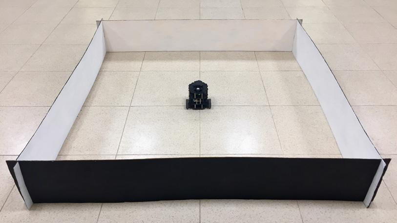
(a)Stagewithwhitewalls

(c)Stagewithblackwalls

(b)Dataacquisitonfrom 12(a)

(d)Dataacquisitonfrom 12(c)

Fig.12. Physicalstage.DataacquisitionisbetterinFig. 12(a) thanFig. 12(c)

(a)Behavioroftherobotinthesimulatedstage.

5.Conclusion

(b)Behavioroftherobotintherealstage.

Fig.13. Behavioroftherobotinthesimulatedandrealstage

TheFLCcreatedwiththefuzzylablibraryworks correctlyintheobstacleavoidancetaskwiththeTurt‑ leBot3robot.Infutureworkmorecomplexcontrol‑ lerscanbedesignedtoworkinmorecomplexstages, implementingoptimizationalgorithmsandevaluating theef�iciencyinsometasks.Forthesimplicityofthe stagecreated,themanipulationofthelinearvelocity wasnotconsideredbutinmorecomplexstagesthede‑ terminationofthelinearvelocitycouldbeconsidered.

Reinforcementlearning(RL),anareaofmachine learning,isacomputationalapproachtounderstan‑ dingandautomatinggoal‑directedlearningandde‑ cisionmaking[15].ManyoftheRLalgorithmssuch asQ‑Learning[16]havebeenusedtooptimizefuzzy logiccontrollers,startingwiththeadaptationofthe Q‑learningalgorithmforfuzzyinferencesystemsby Glorennec[8]andBerenji[2]andmorerecentworks [3–5]forcontrolrobotnavigation.Forthesereasons,

itsuseinfutureworkswithuseofthefuzzylablibrary andtheROSplatformhasbeencontemplated.

ACKNOWLEDGEMENTS

WewouldliketoexpressourgratitudetotheCONA‑ CYTandTijuanaInstituteofTechnologyforthefacili‑ tiesandresourcesgrantedforthedevelopmentofthis research.

Notes

1 �apertutorialfortheenvironmentcon�iguration https://github.com/ITTcs/fuzzylab/tree/master/ tutorials/fuzzylab_paper

2 Referencetutorial http://emanual.robotis.com/docs/en/ platform/turtlebot3/machine_learning/

AUTHORS

EduardoAvelar∗ –TijuanaInstituteof Technology,Tijuana,Mexico,e‑mail:edu‑ ardo.avelar17@tectijuana.edu.mx.

OscarCastillo –TijuanaInstituteofTechnology,Tiju‑ ana,Mexico,e‑mail:ocastillo@tectijuana.mx.

JoséSoria –TijuanaInstituteofTechnology,Tijuana, Mexico.

∗ Correspondingauthor

REFERENCES

[1] E.Avelar.“fuzzylab”. https://github.com/ ITTcs/fuzzylab,2019,Accessedon:2020‑05‑ 28.

[2] H.R.Berenji,“Fuzzyq‑learning:anewapproach forfuzzydynamicprogramming”,vol.1,1994, 486–491,10.1109/FUZZY.1994.343737.

[3] H.Boubertakh,M.Tadjine,andP.‑Y.Glorennec,“A newmobilerobotnavigationmethodusingfuzzy logicandamodi�iedq‑learningalgorithm”, Jour‑ nalofIntelligent&FuzzySystems,vol.21,no.1 and2,2010,113–119,10.3233/IFS‑2010‑0440.

[4] L.CherrounandM.Boumehraz,“Intelligentsys‑ temsbasedonreinforcementlearningandfuzzy logicapproaches,”applicationtomobilerobo‑ tic””,2012,1–6,10.1109/ICITeS.2012.6216661.

[5] L.Cherroun,M.Boumehraz,andA.Kouzou, “Mobilerobotpathplanningbasedonopti‑ mizedfuzzylogiccontrollers”,2019,255–283, 10.1007/978‑981‑13‑2212‑9_12.

[6] Y.DuanandXin‑Hexu,“Fuzzyreinforce‑ mentlearninganditsapplicationinro‑ botnavigation”,vol.2,2005,899–904, 10.1109/ICMLC.2005.1527071.

[7] M.Faisal,R.Hedjar,M.A.Sulaiman,andK.Al‑ Mutib,“Fuzzylogicnavigationandobstacleavoi‑ dancebyamobilerobotinanunknowndyn‑ amicenvironment”, InternationalJournalofAd‑ vancedRoboticSystems,vol.10,no.1,2013,37, 10.5772/54427.

[8] P.Y.GlorennecandL.Jouffe,“Fuzzyq‑learning”. In: Proceedingsof6thInternationalFuzzySy‑ stemsConference,vol.2,1997,659–662vol.2, 10.1109/FUZZY.1997.622790.

[9] L.MarkowskyandB.Segee,“Theoctave fuzzylogictoolkit”.In: 2011IEEEInterna‑ tionalWorkshoponOpen‑sourceSoftware forScienti�icComputation,2011,118–125, 10.1109/OSSC.2011.6184706.

[10] J.M.Mendel, UncertainRule‑BasedFuzzySys‑ tems:IntroductionandNewDirections,Springer, 2017.

[11] S.M.Raguraman,D.Tamilselvi,andN.Shivaku‑ mar,“Mobilerobotnavigationusingfuzzylogic controller”.In: 2009InternationalConferenceon

Control,Automation,CommunicationandEnergy Conservation,2009,1–5.

[12] P.Reignier,“Fuzzylogictechniquesformobile robotobstacleavoidance”, RoboticsandAutono‑ mousSystems,vol.12,no.3,1994,143–153, 10.1016/0921‑8890(94)90021‑3.

[13] A.Saf�iotti,“Theusesoffuzzylogicinautono‑ mousrobotnavigation”, SoftComputing,vol.1, no.4,1997,180–197,10.1007/s005000050020.

[14] R.Siegwart,I.R.Nourbakhsh,andD.Scaramuzza, IntroductiontoAutonomousMobileRobots,The MitPress,2011.

[15] R.S.SuttonandA.G.Barto, ReinforcementLear‑ ning:AnIntroduction,TheMitPress,2018.

[16] C.J.C.H.WatkinsandP.Dayan,“Q‑learning”, MachineLearning,vol.8,no.3,1992,279–292, 10.1007/BF00992698.

[17] L.A.Zadeh,“Fuzzysets”, InformationandCont‑ rol,vol.8,no.3,1965,338–353,10.1016/S0019‑ 9958(65)90241‑X.

[18] L.A.Zadeh,“Fuzzylogic=computingwith words”, IEEETransactionsonFuzzySystems,vol. 4,no.2,1996,103–111,10.1109/91.493904.

Toward the Best Combination of Optimization with Fuzzy Systems to Obtain the Best Solution for the GA and PSO Algorithms Using Parallel Processing

Submitted: 20th December 2019; accepted: 30th March 2020

Fevrier Valdez, Yunkio Kawano, Patricia Melin

DOI: 10.14313/JAMRIS/1-2020/7

Abstract: In general, this paper focuses on finding the best configuration for PSO and GA, using the different migration blocks, as well as the different sets of the fuzzy systems rules. To achieve this goal, two optimization algorithms were configured in parallel to be able to integrate a migration block that allow us to generate diversity within the subpopulations used in each algorithm, which are: the particle swarm optimization (PSO) and the genetic algorithm (GA). Dynamic parameter adjustment was also performed with a fuzzy system for the parameters within the PSO algorithm, which are the following: cognitive, social and inertial weight parameter. In the GA case, only the crossover parameter was modified.

Keywords: Genetic Algorithms, Particle Swarm Optimization, Fuzzy Logic, Parallel Processing

1. Introduction

In this paper, we are dedicated to finding the best configuration that will help us obtain the minimum error for the pair of optimization algorithms that we use. We consider different sets of fuzzy system rules and also with the integration of different migration blocks to share information between the two algorithms.

Also, some benchmark functions are too complex, and they can take too long for the optimization algorithms, so we configure the algorithms to be used in parallel and thereby improve the runtime. This allows us to be able to use the migration blocks so that information is shared between each of the algorithms and to find the global minimum in less time.

The biggest problem with metaheuristic algorithms is that when they are searching there comes a time when they could stagnate and not reach the specific global minimum of each benchmark function. That is why we combine several strategies to avoid this situation.

As for the strategies to improve the methods, we refer to the dynamic adaptation of parameters for each algorithm, and also to the migration blocks that

allow us to find a global minimum between the two algorithms (GA and PSO).

Previously, some other researchers have worked with the same optimization algorithms as us, but some of them have focus on the reduction of the runtime of the algorithms, others use algorithm with dynamic parameters adjustment with fuzzy systems. As in our previous paper in which we were working with the improvement of the performance of the same way to the algorithms of PSO and GA, but of individuals form each and with the use of processing inside of GPU (Graphics Processing Unit). In which we focus on reducing runtime [1].

In the current case in which we take care of finding the global minimum in less time with the integration of GPUs, we can find other people in the research community who work on similar research[2]–[5]. Also, some researchers have dedicated themselves to the use of fuzzy systems to find the parameters and others researchers are working with the use the others topologies of each algorithm to reach the best global minimum [6].

In comparison to the other mentioned researchers, the difference of our work is that we combine different strategies to find the best solution for each of the benchmark functions, such as: the parallel execution that allows us to share information with the migration blocks between the optimization algorithms [7]–[9].

Below a summary of each of the sections contained in the paper is presented. Within Section 2 there are three subsections which are part of the theoretical framework we use, such as concepts and pseudocode of the GA and PSO algorithms, and as a third subsection, our contribution is better described, which is, the joint version of the PSO and GA in parallel with the description of the different fuzzy systems and the migration blocks that were used. Section 3 shows the experiments we performed and the results obtained from them, shown separately from each of the two cases used where one focused on the use of fuzzy systems of one input and one output, as well as one input and two outputs. Finally, in Section 4, we find our conclusions based on the results obtained.

2. Theory of the Optimization Algorithms and Improvement Strategies Used

In this section you will see all the theory related to the optimization algorithms and strategies used where it will be divided by subsections for better understanding.

2.1. Genetic Algorithms

Once the pseudocode of the genetic algorithm is shown, Genetic algorithms (GA) are algorithms that are based on natural selection, where we can find the inherited characteristic of the parent chromosomes to the children, where the individuals are eliminating the weakest chromosomes according to the principles of Charles Darwin were the fittest survives. As in nature, the rivalry between people for scarce resources results in the fittest people ruling over the weakest [2], [4], [10].

In Figure 1 the pseudocode for the genetic algorithm is presented.

Fig. 1. Pseudocode of the Genetic Algorithm

The Figure 1, represent a cycle with an analysis of the process than can be parallelized and then can be implemented on the video card for improving runtime. The first process that is sent to the video card is “Assign fitness value to entire population” and these “Select the best solution”. The code modification is very small, but with that, you can get an improvement in the runtime.

2.2. Particle Swarm Optimization

Particle Swarm Optimization (PSO) is apopulation-basedstochasticoptimizationtechniquedevelopedbyEberhartandKennedyin1995, inspired by social behavior of bird flocking or fish schooling [7], [11]–[14].

PSO has many processes similar to those that work with genetic algorithms. This algorithm initiates a swarm of random particles, where each of the

contained particles could be a solution to the problem that is being worked on. These possible solutions are evaluated in each of the iterations that we have.

Figure 2 shows the pseudocode of the PSO algorithm. [6], [14]–[16]:

Fig. 2. Pseudocode of PSO algorithm

The following equation represents the update of the velocity vector of each particle in each iteration k.

A more detailed description of each factor is made below:

vik = Is the velocity of the particle i in the iteration k w = Is the inertial factor.

∅1, ∅2 = The learning ratios (weights) that control the cognitive and social components.

rand1, rand2 = The random numbers between 0 and 1. x i k = Current position of particle i in iteration k. pBesti = Best position (solution) found by the particle i so far gi represents the position of the particle with the pBest_fitness of the environment of gi(localbest). Eq. 2.

2.3. Parallel PSO and GA

The parallel PSO and GA is formed by the combination of the algorithms described above, to create a parallel version to be able to integrate a migration block, which allows us to generate diversity in the populations of each of algorithms. The algorithms share among them, either, the entire population of the best individuals. A fuzzy system is also proposed to dynamically adjust the PSO and some GA parameters [8], [12], [17], [18].

Although we don’t use graphics cards in our algorithm, certain articles helped us to know what parameters of the algorithm we can use to share information in parallel with another algorithm.

Figure 3 illustrates the flow of information in proposed method.

Figure 3 shows the flow chart that is used to obtain the results of our experiments. Which is composed of a block in which the main parameters are defined for each of the algorithms that are used, after having created the population then it is divided so that each of the algorithms works. From there each one of the algorithms begins to work simultaneously and each performs its respective processes. We can see in the center of Figure 3 that there is a migration block which refers to each of the following blocks (Figures 4, 5 and 6). On each of the sides of the diagram the union point number 3 is observed, which joins the block that is in the lower-left part of Figure 3 in which the dynamic adjustment of parameters is made according to the fuzzy systems which are shown in Figures 7, 8, 9, 10 and 11 [16], [19]–[23].

2.4. Migration

Blocks

The migration blocks are more focused on improving the results obtained by the genetic algorithm, which migrates individuals between the two algorithms to add more diversity within each population [24].

5.

In Figure 5 the migration block number 2 is shown in which the same population change is made as the previous block, but now it is activated every certain number of iterations.

Finally, in Figure 6 is observed that the best solutions are found for each of the populations, these are compared and only the best ones are exchanged.

Only the parameters of the PSO variables were adjusted, which are the cognitive, social and the inertial weight parameters. This is why in each of the fuzzy systems shown below, only the rules of each one change.

2.5.

Dynamic Adjustment of Parameters With Fuzzy Systems

CASE 1 WITH FUZZY SYSTEMS OF ONE INPUT AND ONE OUTPUT:

The fuzzy systems used for dynamic adjustment are the following models.

In Figure 7 the set of rules that are used in the fuzzy system type A is shown, in this case, it’s the same membership functions for the cognitive and social parameters.

In Figure 4 the migration block number 1 is shown in which the comparison is made among all the PSO particles and all GA individuals, in the case that the individuals are greater than the particles a population change is made between the algorithms.

In Figure 8 the membership functions of the cognitive parameter are varied.

Fig. 3. Parallel PSO and GA

Fig. 4. Migration block number 1

Fig.

Migration block number 2

Fig. 6. Migration block number 3

Fig. 7. Rules for each fuzzy systems type A

Fig. 8. Rules for fuzzy system type B

In Figure 7, the used rules are the same for all variables (cognitive, social and inertial weight parameters). In Figure 8, the rules change for the fuzzy systems of the cognitive parameter. Finally, in the case of Figure 9, it is similar to the previous one, but now the rules are changed for the social parameter. CASE 2 WITH FUZZY SYSTEMS OF ONE INPUT AND TWO OUTPUTS:

The following fuzzy systems refer to those in case 2 of the experiments that are composed of one input and two outputs.

In Figure 10, each of the rules is like the rules used in Figure 7.

In Figure 11, each of the rules is like the rules used in Figure 8.

12.

In Figure 12, each of the rules is like the rules used in Figure 9.

In Figure 13, are presented the rules that contain the fuzzy system of one input and two outputs. The output variables are the cognitive and social parameters of the PSO algorithm. These are influenced by the input variable, which is the number of iterations.

In Figure 14, in this case, all the possible rules that can be created for the fuzzy system of one input and two outputs with three membership functions are used. Different number of rules was used to experiment if they influence the obtained results.

3. Experiments and Results

The computer on which the experiments were made has the following hardware components. It has an Intel Core i7-4770 to 3.4 GHz with 4 cores and 8 threads, and the amount of 16 gigabytes of memory RAM (Random Access Memory) to 1600 MHz.

The benchmark functions that were use are in the following figure.

Figure 15 shows the benchmark mathematical functions that were used for the experiments, the first column is the identification list of each the functions, on the other hand, all functions have the objective of reaching zero[25], [26].

The results shown below are made based on a combination of different fuzzy systems varying

Fig. 9. Rules for fuzzy system type C

Fig. 10. Rules for fuzzy system type D

Fig. 11. Rules for fuzzy system type E

Fig.

Rules for the fuzzy system type F

Fig. 13. Nine rules for the fuzzy system

Fig. 14. Twenty-seven rules for the fuzzy system (it is all possible)

the number of rules, as well as different migration blocks.

Fig. 15. List of benchmark functions

Tab. 1. PSO and GA parameters used PSO and GA parameters

Population 100

Dimensions

5, 10, 20, 40, 80, 160, 320, 640, 1280

Iterations / Generations 1000

Cognitive parameter Dynamic

Social parameter Dynamic

Inertial weight Dynamic

Percentage of Crossing 0.8

Assignment Fitness Value Ranking

Selection Universal Stochastic Sampling

Recombination

Multipoint crossing

Mutation (0.7 / Chrome length)

3.1. Experiments for CASE 1 With One Input and One Output

This refers to the combination of the two optimization algorithms with dynamic adjustment of parameters with a fuzzy system for each of the variables. Each of the following figures is equivalent to a set of experiments of each benchmark functions used.

Figure 16 to 23 illustrate the results of the experiments for case 1 that includes a comparison between the different configurations of fuzzy systems (Figures 7, 8 and 9) as well as the different migration blocks (Figures 4, 5 and 6). Zero refers to the fact that it does not include a migration block.

In Figure 16 is observed that in the CASE-1-B-1, which the case of one input and one output is where the fuzzy system is of type B and the migration block is the number 1, better results were obtained for all the dimensions that were used, which are from 5 to 1280 dimensions.

It can be see that in the cases where the number 1 indicates that block 1 was used are those that obtain a lower value, especially case 1 with fuzzy system type B.

Fig. 16. Comparison of the results of the different combination used in Case 1: with the fuzzy systems A, B and C, as well as with the integration of migration blocks 0, 1, 2 and 3. These evaluating the benchmark function 1

Fig. 17. Comparison of the results of the different combinations used in Case 1: with the fuzzy systems A, B and C, as well as with the integration of migration blocks 0, 1, 2, and 3. These evaluating the benchmark function 2

In the same way, Figure 17 shows that the fuzzy system type B with the migration block 1 is the winner for the benchmark function number 2 (Figure 15).

Fig. 18. Comparison of the results of the different combinations used in Case 1: with the fuzzy systems A, B and C, as well as with the integration of migration blocks 0, 1, 2 and 3. These evaluating the benchmark function 3

In Figure 18, the values found are extremely high, but as in the previous case type B is the winner, although it does not reach zero, it is less than the other ones in this figure. The highest value is around of 70,900,000 for GA and the lowest value is around 360,000 for PSO, it’s a great difference this value is

when we working with 1280 dimensions and configuration “CASE-1-B-2”. But if we are running the algorithm with other configuration as “CASE-1-B-1” we obtain a great difference with values around 2,900 where we working with 1280 dimensions.

In Figure 19, in other cases we saw that the combination with the migration block improved the results but for the benchmark function number 4, we could notice that this same migration block was beneficial for all the fuzzy systems used.

Fig. 19. Comparison of the results of the different combinations used in Case 1: with the fuzzy systems A, B and C, as well as with the integration blocks 0, 1, 2 and 3. These evaluating the benchmark function 4

In Figure 20, good results are observed in the same cases as the previous figure although the values close to zero are at low dimensions. The best values obtained in this case for the benchmark function 5 are around 1,300 for the “Case-1-B-1”.

Fig. 20. Comparison of the results of the different combinations used in Case 1: with the fuzzy systems A, B and C, as well as with the integration blocks 0, 1, 2 and 3. These evaluating the benchmark function 5

For function 6, in Figure 21, good results are obtained with low dimensions because when we are working with 1,280 dimensions the results obtained are around 1,100.

In function 7 in Figure 22, it is a good result with “Case-1-B-1”. The best solutions are between 0 and 0.5 for all dimensions used and this is due to the benchmark function.

In Figure 23, the minimum values is between 0 and 0.28 for function 8. We can note that the results using block 1 are the best.

Fig. 21. Comparison of the results of different combination used in Case 1: with the fuzzy systems A, B and C, as well as with the integration of migration blocks 0, 1, 2 and 3. These evaluating the benchmark function 6

Fig. 22. Comparison of the results of different combination used in Case 1: with the fuzzy systems A, B and C, as well as with the integration of migration blocks 0, 1, 2 and 3. These evaluating the benchmark function 7

Fig. 23. Comparison of the results of different combination used in Case 1: with the fuzzy systems A, B and C, as well as with the integration of migration blocks 0, 1, 2 and 3. These evaluating the benchmark function 8

The following figures between Figure 24 to Figure 31 show the results of case 2 that focuses on the use of fuzzy systems of one input and two outputs.

3.2. Experiments for CASE 2 With One Input and Two Outputs

In the same way that in case 1 it can be observed that the use of the migration blocks is the one with the best results. In figure 24, the winning column is “Case-2-B-1” although it goes hand in hand with the “Case-2-B-0”

which is the one that does not integrate migration block. The best value is around 5 for these columns.

Fig. 24. Comparison of the results of the different combinations used in Case 2: with fuzzy systems A, B and C, as well as with the integration of migration blocks 0, 1, 2 and 3. These evaluation the benchmark function 1

Fig. 25. Comparison of the results of the different combinations used in Case 2: with fuzzy systems A, B and C, as well as with the integration of migration blocks 0, 1, 2 and 3. These evaluations the benchmark function 2

In Figure 25, the comparison is made between all the versions of case 2, which shows as a result that the cases where fuzzy type B is used, with the use of migration block 1 as well as where no block is used, being block 1 the one that gets numbers closer to zero when we are working with low dimensions, but if we work with high dimensions the results go up to almost 3,000.

Fig. 26. Comparison of the results of the different combinations used in Case 2: with the fuzzy systems A, B, and C, as well as with the integration of migration blocks 0, 1, 2, and 3. These evaluating the benchmark function 3

In Figure 26, for the experiment of case 2 for the evaluation function 3 it is shown that in the same way as the previous cases the configuration with the case where it uses the migration block 1 is the closest to zero, arriving at the use of 80 dimensions.

Fig. 27. Comparison of the results of the different combinations used in Case 2: with the fuzzy systems A, B, and C, as well as with the integration of migration blocks 0, 1, 2, and 3. These evaluating the benchmark function 4

Evaluating function number 4 in Figure 27, it is shown that in a greater number of configurations the objective of the function that is zero is reached. Although it is observed that in most of the cases is that it is gained by the use of the migration block 1.

Fig. 28. Comparison of the results of the different combinations used in Case 2: with the fuzzy systems A, B, and C, as well as with the integration of migration blocks 0, 1, 2, and 3. These evaluating the benchmark function 5

Figure 28, in this evaluation of function 5, it was not possible to reach zero in any experiment, even though we were working with low dimensions although it was close to the minimum value.

In Figure 29 compared to Figure 28, worse results are observed which are large in value. Even when working up to 1280 dimensions are lower than the results observed in Figure 28.

In Figure 30, the results are very low but it is because it depends on the function with which you are working. At low dimensions, you can get some zeros in the values.

Figure 31, if we compare it with case 1 it can be seen that the values, in general, are a little lower depending of the number of dimensions that are being used.

Fig. 29. Comparison of the results of the different combinations used in Case 2: with the fuzzy systems A, B, and C, as well as with the integration of migration blocks 0, 1, 2, and 3. These evaluating the benchmark function 6

Fig. 30. Comparison of the results of the different combinations used in Case 2: with the fuzzy systems A, B, and C, as well as with the integration of migration blocks 0, 1, 2, and 3. These evaluating the benchmark function 7

Fig. 31. Comparison of the results of the different combinations used in Case 2: with the fuzzy systems A, B, and C, as well as with the integration of migration blocks 0, 1, 2, and 3. These evaluating the benchmark function 8

4. Conclusion

As a general conclusion, after analyzing all the results of the performed experiments out, it can be stated that the use of the parallel algorithm combining PSO and GA with the integration of migration block 1 (Fig. 4) and the used of the fuzzy system type B (Fig. 8), is the most suitable for working at high dimensions.

In certain benchmark functions it was observed that the other types of fuzzy systems were good, but they cannot beat type B.

Regarding the comparison between cases 1 and case 2, the results show that there are very similar although on some situations case 2 wins case 1 and vice versa.

In the case of the fuzzy system of nine and twenty-seven rules, good results were not obtained, we believe that they are too many rules and saturates, giving as output a similar values for all the input modifications to the fuzzy.

Comparing Case 1 and 2 for the experiments, we observed that the global minimum values found are very similar although in some benchmark functions, the results obtained were better, but in other cases the other one won. In cases where nine and twenty-seven rules were used within the fuzzy system, they were not the best, we thought that membership functions were spliced and that is why they did not help and caused them to give the same output value regardless of the value of the input that was used.

As future work we can make use of Type-2fuzzy systems[27]–[32], as well as an algorithm that helps us optimize the rules of fuzzy systems so that they are the most appropriate and help us improve the local minimum found; although this will make the runtime of the experiment is higher, that is why it could also integrate the use of GPU to improve the performance of the parallel algorithm in general.

A CK n OW l EDGEME n TS

The authors would like to thanks CONACYT and Tijuana Institute of Technology for the support during this research work.

AUTHORS

Fevrier Valdez* – Division of Graduate Studies and Research, Tijuana Institute of Technology, Tijuana, Mexico, e-mail: fevrier@tectijuana.mx.

Yunkio Kawano – Division of Graduate Studies and Research, Tijuana Institute of Technology, Tijuana, Mexico, e-mail: monicoyunkio89@gmail.com.

Patricia Melin – Division of Graduate Studies and Research, Tijuana Institute of Technology, Tijuana, Mexico, e-mail: pmelin@tectijuana.mx.

* Corresponding author

R EFERE n CES

[1] Y. Kawano, F. Valdez and O. Castillo, “Performance Evaluation of Optimization Algorithms based on GPU using CUDA Architecture”. In: 2018 IEEE Latin American Conference on Computational Intelligence (LA-CCI), 2018, 1–6, DOI: 10.1109/LA-CCI.2018.8625236.

[2] G. R. Harik, F. G. Lobo and D. E. Goldberg, “The compact genetic algorithm”, IEEE Transactions on Evolutionary Computation, vol. 3, no. 4, 1999, 287–297, DOI: 10.1109/4235.797971.

[3] X. H. Shi, Y. H. Lu, C. G. Zhou, H. P. Lee, W. Z. Lin and Y. C. Liang, “Hybrid evolutionary algorithms based on PSO and GA”. In: The 2003 Congress on Evolutionary Computation, 2003. CEC ‘03, vol. 4, 2003, 2393–2399, DOI: 10.1109/CEC.2003.1299387.

[4] S. Debattisti, N. Marlat, L. Mussi, S. Cagnoni, “Implementation of a Simple Genetic Algorithm within the CUDA Architecture”, GPUs for Genetic and Evolutionary Computation Competition at 2009 Genetic and Evolutionary Computation Conference, 2009.

[5] L. Mussi and S. Cagnoni, “Particle swarm optimization within the CUDA architecture”, 2009.

[6] J. C. Vazquez and F. Valdez, “Fuzzy logic for dynamic adaptation in PSO with multiple topologies”. In: 2013 Joint IFSA World Congress and NAFIPS Annual Meeting (IFSA/NAFIPS), 2013, 1197–1202, DOI: 10.1109/IFSA-NAFIPS.2013.6608571.

[7] F. Olivas, F. Valdez and O. Castillo, “Fuzzy Classification System Design Using PSO with Dynamic Parameter Adaptation Through Fuzzy Logic”. In: O. Castillo and P. Melin (eds.), Fuzzy Logic Augmentation of Nature-Inspired Optimization Metaheuristics: Theory and Applications, 2015, 29–47, DOI: 10.1007/978-3-319-10960-2_2.

[8] F. Valdez, P. Melin and O. Castillo, “Fuzzy control of parameters to dynamically adapt the PSO and GA Algorithms”. In: International Conference on Fuzzy Systems, 2010, 1–8, DOI: 10.1109/FUZZY.2010.5583934.

[9] F. Valdez, P. Melin and O. Castillo, “Fuzzy Logic for Combining Particle Swarm Optimization and Genetic Algorithms: Preliminary Results”. In: A. H. Aguirre, R. M. Borja and C. A. R. Garciá (eds.), MICAI 2009: Advances in Artificial Intelligence, 2009, 444–453, DOI: 10.1007/978-3-642-05258-3_39.

[10] J. Carnahan and R. Sinha, “Nature’s algorithms [genetic algorithms]”, IEEE Potentials, vol. 20, no. 2, 2001, 21–24, DOI: 10.1109/45.954644.

[11] Eberhart and Y. Shi, “Particle swarm optimization: developments, applications and resources”. In: Proceedings of the 2001 Congress on Evolutionary Computation, vol. 1, 2001, 81–86, DOI: 10.1109/CEC.2001.934374.

[12] F. Olivas, F. Valdez and O. Castillo, “Particle swarm optimization with dynamic parameter adaptation using interval type-2 fuzzy logic for benchmark mathematical functions”. In: 2013 World Congress on Nature and Biologically Inspired Computing, 2013, 36–40, DOI: 10.1109/NaBIC.2013.6617875.

[13] J. Kennedy and R. Eberhart, “Particle swarm optimization”. In: Proceedings of ICNN’95 – International Conference on Neural Networks, vol. 4, 1995, 1942–1948, DOI: 10.1109/ICNN.1995.488968.

[14] R. Poli, J. Kennedy and T. Blackwell, “Particle swarm optimization”, Swarm Intelligence, vol. 1, no. 1, 2007, 33–57, DOI: 10.1007/s11721-007-0002-0.

[15] F. Olivas, L. Amador-Angulo, J. Perez, C. Caraveo, F. Valdez and O. Castillo, “Comparative Study of Type-2 Fuzzy Particle Swarm, Bee Colony and Bat Algorithms in Optimization of Fuzzy Controllers”, Algorithms, vol. 10, no. 3, 2017, DOI: 10.3390/a10030101.

[16] F. Valdez, P. Melin and O. Castillo, “Parallel Particle Swarm Optimization with Parameters Adaptation Using Fuzzy Logic”. In: I. Batyrshin and M. G. Mendoza (eds.), Advances in Computational Intelligence, 2013, 374–385, DOI: 10.1007/978-3-642-37798-3_33.

[17] Y. Shi and R. C. Eberhart, “Fuzzy adaptive particle swarm optimization”. In: Proceedings of the 2001 Congress on Evolutionary Computation (IEEE Cat. No.01TH8546), vol. 1, 2001, 101–106, DOI: 10.1109/CEC.2001.934377.

[18] J. Kaur, S. Singh and S. Singh, “Parallel Implementation of PSO Algorithm Using GPGPU”. In: 2016 Second International Conference on Computational Intelligence Communication Technology (CICT), 2016, 155–159, DOI: 10.1109/CICT.2016.38.

[19] F. Valdez, P. Melin and O. Castillo, “An improved evolutionary method with fuzzy logic for combining Particle Swarm Optimization and Genetic Algorithms”, Applied Soft Computing, vol. 11, no. 2, 2011, 2625–2632, DOI: 10.1016/j.asoc.2010.10.010.

[20] A. S. Radhamani and E. Baburaj, “Performance evaluation of parallel genetic and particle swarm optimization algorithms within the multicore architecture”, International Journal of Computational Intelligence and Applications, vol. 13, no. 4, 2014, DOI: 10.1142/S1469026814500242.

[21] Z.-X. Wang and G. Ju, “A parallel genetic algorithm in multi-objective optimization”. In: 2009 Chinese Control and Decision Conference, 2009, 3497–3501, DOI: 10.1109/CCDC.2009.5192490.

[22] Z. Dingxue, G. Zhihong and L. Xinzhi, “On Multipopulation Parallel Particle Swarm Optimization Algorithm”. In: 2007 Chinese Control Conference, 2007, 763–765, DOI: 10.1109/CHICC.2006.4347299.

[23] X. Lai and G. Tan, “Studies on migration strategies of multiple population parallel particle swarm optimization”. In: 2012 8th International Conference on Natural Computation, 2012, 798–802, 10.1109/ICNC.2012.6234614.

[24] H. Pohlheim, “Genetic and Evolutionary Algorithm Toolbox for Matlab”. In: Evolutionäre Algorithmen, 2000, 157–170, DOI: 10.1007/978-3-642-57137-4_6.

[25] J. G. Digalakis and K. G. Margaritis, “An Experimental Study of Benchmarking Functions for Genetic Algorithms,” International Journal of Computer Mathematics, vol. 79, no. 4, 403–416, 2002, DOI: 10.1080/00207160210939.

[26] “GEATbx: Example Functions (single and multiobjective functions) 2 Parametric Optimization”. H. Pohlheim, http://www.geatbx.com/docu/fcnindex-01.html. Accessed on: 2020-05-28.

[27] E. Bernal, O. Castillo, J. Soria and F. Valdez, “Interval Type-2 fuzzy logic for dynamic parameter adjustment in the imperialist competitive algorithm”. In: 2019 IEEE International Conference on Fuzzy Systems (FUZZ-IEEE), 2019, 1–5, DOI: 10.1109/FUZZ-IEEE.2019.8858935.

[28] J. R. Castro, O. Castillo and P. Melin, “An Interval Type-2 Fuzzy Logic Toolbox for Control Applications”. In: 2007 IEEE International Fuzzy Systems Conference, 2007, 1–6, DOI: 10.1109/FUZZY.2007.4295341.

[29] R. Martinez, A. Rodriguez, O. Castillo and L. T. Aguilar, “Type-2 Fuzzy Logic Controllers Optimization Using Genetic Algoritms and Particle Swarm Optimization”. In: 2010 IEEE International Conference on Granular Computing, 2010, 724–727, DOI: 10.1109/GrC.2010.43.

[30] N. C. Long and P. Meesad, “Meta-heuristic algorithms applied to the optimization of type-1 and type 2 TSK fuzzy logic systems for sea water level prediction”. In: 2013 IEEE 6th International Workshop on Computational Intelligence and Applications (IWCIA), 2013, 69–74, DOI: 10.1109/IWCIA.2013.6624787.

[31] P. Melin, J. Urias, D. Solano, M. Soto, M. Lopez and O. Castillo, “Voice Recognition with Neural Networks, Type-2 Fuzzy Logic and Genetic Algorithms”, Engineering Letters, vol. 13, no. 2, 2006.

[32] F. Gaxiola, P. Melin, F. Valdez, J. R. Castro and O. Castillo, “Optimization of type-2 fuzzy weights in backpropagation learning for neural networks using GAs and PSO”, Applied Soft Computing, vol. 38, 2016, 860–871, DOI: 10.1016/j.asoc.2015.10.027.

Exploring Random Permutations Effects on the Mapping Process for Grammatical Evolution

Submitted: 20th December 2019; accepted: 30th March 2020

Blanca Verónica Zúñiga, Juan Martín Carpio, Marco Aurelio Sotelo-Figueroa, Andrés Espinal, Omar Jair Purata-Sifuentes, Manuel Ornelas, Jorge Alberto Soria-Alcaraz, Alfonso Rojas

DOI: 10.14313/JAMRIS/1-2020/8

Abstract: Grammatical Evolution (GE) is a form of Genetic Programming (GP) based on Context-Free Grammar (CF Grammar). Due to the use of grammars, GE is capable of creating syntactically correct solutions. GE uses a genotype encoding and is necessary to apply a Mapping Process (MP) to obtain the phenotype representation. There exist some well-known MPs in the state-of-art like Breadth-First (BF), Depth-First (DF), among others. These MPs select the codons from the genotype in a sequential manner to do the mapping. The present work proposes a variation in the selection order for genotype’s codons; to achieve that, it is applied a random permutation for the genotype’s codons order-taking in the mapping. The proposal’s results were compared using a statistical test with the results obtained by the traditional BF and DF using the Symbolic Regression Problem (SRP) as a benchmark.

Keywords: Grammatical evolution, mapping process, symbolic regression

1. Introduction

Genetic Programming (GP) is an Automatic Programming (AP) technique proposed by Koza [1]. It aims the automatic construction of solutions to different types of problems. One way to obtain syntactically correct solutions is by using grammars that restrict the search space [2, 3]. Grammars provide a mechanism that can be used to describe complex structures and define what can be done [4]. Variants which are grammar-based are the second most commonly used variations of GP [5].

Grammatical Evolution (GE) [6] is a GP based form that uses an integer string and a grammar in a genotype-phenotype mapping to obtain syntactically correct and feasible sentences [7]. Unlike GP, GE performs the evolutionary process in the linear genotype rather than the solution [6]. The Mapping Process (MP) is GE’s component that allows generating solutions (phenotypes) that are guaranteed to be syntactically correct from an integer string (genotype) [8]. This MP can be seen as an abstraction of the DNA, is the conversion of a chromosome (genotype) to a solution (phenotype) [9].

The original MP used in GE was the Depth-First (DF) MP [6]. DF creates the phenotype by taking in linear order one codon value to select one grammar’s production rule applying an equation. Breadth-First (BF) MP [10] was proposed later. The only difference between these two MPs is the order in which the expansion is carried out.

DF and BF are considered the classic MPs, and both use a Backus Naur Form Grammar (BNF-Grammar); since then, many other approaches have been proposed, like the πGrammatical Evolution (πGE) [11], it employs two codons rather than just one: the first codon is used to select the non-terminal to expand (main difference with the classic MPs), and the second codon is used in the same way as the last MPs to select a production rule from the grammar; the Tree-Adjunct Grammatical Evolution (TAGE) [12] uses a tree-adjunct grammar instead of a BNF-Grammar to create the phenotype; the Univariate Model-Based Grammatical Evolution (UMBGE) [13] uses probabilistic context-free grammars and replaces the original genetic operators with the sampling from the distribution of the best solutions; Structured Grammatical Evolution (SGE) [14] uses a different genotypic representation for GE, where each gene is explicitly linked to a non-terminal of the grammar with the purpose of increasing locality; among others. There exist some studies about the performance of these different MPs [15, 16, 10] used to solve various types of problems, such as the Symbolic Regression Problem (SRP), The Santa Fe Ant Trail, and the Evenfive Parity Problem. In the classic MPs, the mapping is performed by taking each integer value of the genotype (called codon), and an equation to choose the corresponding production rule. It is created a derivative tree from this process, and the solution taken from it. The order-taking for the genotype’s codons in the classic MPs DF and BF is sequential.

In this paper, we propose a modification in the order-taking of the genotype’s codons for the MPs DF and BF. The obtained results are compared with these traditional MPs applied to the SRP using a statistical test. The paper is structured as follows: Section 2 gives a brief introduction to GE and its components, in Section 3 is presented the proposed approach, the selected setup that was used in the experiments is explained in Section 4; Section 5 presents the obtained results and the statistical analysis, and, finally the conclusions and future work are discussed in Section 6.

2. Grammatical Evolution

GE is a variant of GP that takes inspiration from the biological evolutionary process (a comparative is shown in Figure 1), in GE the DNA is represented as an integer string; to replicate the process, GE uses an MP and a type of grammar to produce the phenotypic solution [6].

Fig. 1. Comparison between the GE approach and a biological genetic system [6]

Traditionally, a BNF-Grammar is used to create syntactically correct solutions [6]. The BNF-Grammar provides the necessary rules to produce the phenotype according to the specific problem that is trying to solve [17]. GE has three main components [18], but for the aim of this work, it has been added the MP as the fourth component. Figure 2 presents the used methodology for GE, it needs four main components: the Problem Instance, a BNF-Grammar, the Search Engine, and the MP.

Due to the modular nature of GE, each one of the components used in GE can be switched [19], from the Problem Instance to the MP.

GE produces as an output a phenotype, which represents the solution found, later, this solution is evaluated with the objective function, and the process continues until the stopping condition is met. The Algorithm 1 shows GE’s algorithm.

2.1. Problem Instance

The Problem Instance refers to the type of issue that is trying to get solved. For example, problems like the Bin Packing Problem (BPP) [18], Even-5-parity

[15, 10], the Santa Fe Ant Trail (SFAT) problem [15, 10], Data Classification [20], the design of the topology of Artificial Neural Networks [21, 22], the Flexible Job Shop Scheduling Problem [23], and the SRP [24, 25, 26, 15] have been tried to get solved with GE.

The Problem used in the present work is SRP, explained in Section 2.1.1.

Symbolic Regression Problem. The SRP [1] is one of the most requested problem domains in the GP community [5]. Techniques like GP [27, 28] and GE [24] have been used to solve such task.

SRP intends to find a mathematical expression that represents (with the minimal error) a given set of data that takes as a base the rules of accuracy, simplicity, and generalization [28]. The obtained mathematical expression can be seen as a function that takes the values of the variables as an input and returns an output [1].

2.2. Backus Naur Form Grammar

BNF-Grammar is a type of grammar employed in GE. The next tuple form this type of grammar [2]:

G = {NT, T, R, S} where:

NT is the set of non-terminal symbols. T is the set of terminal symbols.

R corresponds to the production rules.

S corresponds to the start symbol, S ∈ NT.

Initially, a BNF-Grammar must be defined. This grammar specifies the structure that the possible solutions produced by GE must have.

The BNF-Grammar consist of two types of symbols, the non-terminal (NT) symbols, and the terminal (T) symbols. The first type can be expanded into NT or T symbols (according to the production rules of the grammar); the second type corresponds to the set that contains the symbols that are allowed to appear in the final expression. The last one, the start symbol S indicates where is the starting point in the grammar. As an example, in Grammar 1 the NT is the set described by NT = {<e>, <v>, <o>}, and the set of T is described by T = {X, Y, -, +}.

Fig. 2. Used GE’s methodology based on [18]

Fig. 2. Used GE's methodology based on [18]

Each NT has its corresponding production rules (separated by the symbol “ ”), and each production rule is separated by the symbol “|”.

Grammar 1. Example of a simple BNF-Grammar

2.3.

Search Engine

The main intention of the Search Engine (SE) is to evolve the candidates throw a search algorithm to find the best one [6]. To achieve that, the SE evaluates each candidate with the objective function, this evaluation is called fitness and represents the performance of an individual to solve a determinate problem [29, 30, 6].

Genetic Algorithm. In this work is used the Genetic Algorithm (GA) as SE. The reason to use the GA is that it represents the canonical search algorithm used in GE’s initials [6]. GA is a metaheuristic inspired by the evolutionary process proposed in its initials by Darwin [31]; Holland later proposed the algorithm for the GA [32]. Algorithm [2] shows the process of GA.

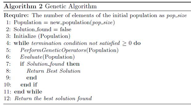
2.4.

Mapping Process

The MP is the procedure of creating a derivative tree with the help of a grammar. GE uses the Equation 1, a grammar and the genotype (an integer string) to transform the genotype into a phenotype. In Figure 3 is shown an example of this process.

ProdRule = CodonVal % NumOfProdRule for the NT (1)

To exemplify each MP, it is used the example Grammar 1, and the following genotype:

Genotype = 2,12,7,9,3,15,23,1,11,4,6,13,2,7,8,3,35,19,2,6

Depth-First Mapping Process. The DF MP [6] starts from the start symbol and makes the corresponding expansion by taking the left-most NT in the derivative tree. Equation 1 is used to choose the appropriate production rule, by substituting the corresponding codon value of the genotype and the number of production rules of the current NT. This process is presented in Figure 4 (the numbers out of the parenthesis indicate the expansion order in the derivative tree). In the example we start with the NT <e>; using the Eq. 1 we substitute the corresponding values, taking the first codon value: 2, and the number of production rules for <e>: 2, the result is 0, which indicates that the next production rule is the one that corresponds to the position zero. And now, there are three new available NTs in the list: <e>, <o> and <e>; the next NT to expand is <e>. We repeat this same process until there no more NTs remain in the derivative tree. The phenotype is obtained by traversing the end nodes of the expansion tree. The obtained phenotype for this example is “Y-Y-X”. DF is considered the classic MP for GE [6]. The corresponding algorithm for this MP is shown in Algorithm 3.

Breadth-First Mapping Process. The second MP used in this work is the BF MP [10]. This MP distinguishes from the DF only by the order in which the expansion is executed. It uses the same equation to choose the corresponding production rule (Eq. 1) but makes the expansion level by level in a left to right order.

In the same way as the last process, the mapping initiates with the start symbol <e> (specified in the grammar). Applying the module rule the corresponding expansion is <e><o><e>. The expansion continues

Fig. 3. Used GE's methodology based on [18]

Fig. 3. Used GE’s methodology based on [18]

by taking every NT in a level of the tree from left to right until no more NTs remain. In this case, the retrieved phenotype is “Y-X-Y”. The example of this process is shown in Figure 5, and its corresponding algorithm in Algorithm 4.

3. Proposed Approach

In the classical MPs BF and DF, the codons are taken sequentially. It means that each codon value is used one by one in order of appearance as is shown in the example Figure 6. The figure shows the genotype (represented as an integer string in the first row), its corresponding sequential order-taking for the codons (second row), the BNF-Grammar employed, and the correspondent derivative process. In this last, the list of NTs is placed at the left side, and on the right side is indicated the order in which the codons are taken. Before the “→” symbol, the corresponding substituted values are shown for the Equation 1.

In the proposed approach, we change the order-taking for the codons in the MPs BF and DF. To set this order-taking is employed a random permutation. Figure 7 shows an example of the proposal used in the DF MP. The figure shows the genotype (represented as an integer string in the second row), its corresponding order-taking for the codons (third row), the original index for the genotype (first row), the BNF-Grammar employed, and the derivative process.

6. Example of the transformation genotype-tophenotype using the classic MP DF

Fig. 4. Example of Depth-First Mapping Process [6]

Fig. 5. Example of Breadth-First Mapping Process

Fig.

In this last, the list of NTs is placed at the left side, and on the right side is indicated the order in which the codons are taken. Note that it is used the permutation (perm) to choose the index of the gen. After the “→” symbol, the corresponding substituted values are shown for the Equation 1.

4. Experimental Analysis

4.1.

Benchmark Functions

Experiments were performed to evaluate the performance of the proposal using a set of ten functions of the SRP. Table 1 shows the ten functions used in the experimental analysis. These functions were taken from [24, 33].

Tab. 1. Symbolic Regression functions used as instance set [24, 33]

Function Fit Cases

F1 32=+ + xx x

F2 43 2 =+ ++ xx xx

F3 54 32 =+ ++ + xx xx x

F4 65 43 2 =+ ++ ++ xx xx xx

Fs in cos 5 2 1 =− () ()xx

Fsin sin 6 2 =+ () ()xx x

F7 2 11=+() ++()loglogxx

20 random points x ∈ [-1,1]

20 random points x ∈ [0,2]

F8 = x 20 random points x ∈ [0,4]

F10 2 = () () sincosxy

F9 2 = () + () sinsinxy 200 random points ∈ [-1,1], x ∈ [-1,1], y ∈ [-1,1]

4.2.

Parameter Setup

We employed a GA as a Search Engine for the GE in the experiments to make the evolutionary process of the genotypes. The used parameters were set empirically. Table 2 shows the corresponding parameter values for the GA.

Grammar 2 shows the grammar used in the experiments. This grammar was taken from [24].

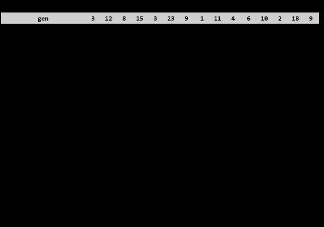
Fig. 7. Example of the transformation genotype-tophenotype using the proposal with the DF MP

Tab. 2. Parameter settings used in the GA

Parameter Value

Population size

300 individuals

Initial genotype length 100 codons (random init)

Stopping condition 25,000 function calls

Selection Method Binary tournament

Crossover Operator 2 points

Mutation Operator Flip bit

Replacement Strategy Generational with elitism (best individual)

Tab. 3. Medians and variances for the best fitness in classical MPs (DF and BF) and these MPs using the proposal applied to the SRP

The Mean Root Squared Error (MRSE) given by Equation 2 was used as objective function to evaluate the candidate expressions obtained by the GE. MRSE yF x N ii i N = = ∑ (( ))2 1 (2)

where:

N is the number of data points. yi is the real value. F(xi) corresponds to the obtained value.

5. Results and Statistical Analysis

33 individual experiments were performed to evaluate the performance of the proposal. Table 3 shows the obtained results (the median and variance of the best fitness values achieved) using the classical MPs and the MPs with the proposal to solve each function in Table 1.

A Friedman non-parametrical test was used to know if there exists a significant difference between the proposal and the classical MPs. The obtained p-value for the medians of the best fitness was 0.5163. The same test was performed for the variances of the best fitness. The obtained p-value was 1.87E-05. Table 4 shows the average ranking obtained with the variances.

6. Conclusion

A new approach for the order-taking of codons in the MPs Depth-First and Breadth-First applied to the SRP was proposed. The obtained results were compared with the well-known MPs Depth-First and Breadth-First using the Friedman non-parametrical test.

Derived from the obtained results with the Friedman test we could conclude that there is no evidence to differentiate between the performance (regarding with the median) of the standard MPs, and this same MPs using the proposal.

However, there is statistical evidence to discern between the performance of the MPs concerning the variance. The results indicate that the proposal provides the algorithms of BF and DF MPs with higher consistency.

As future work, it is proposed to search for a methodology that helps to find the best permutation for the order-taking of the codons in GE’s MPs.

A C k N owl E d GEMENTS

The authors want to thank National Council for Science and Technology of Mexico (CONACyT) through the scholarship for postgraduate studies: 703582 (B. Zuñiga) and the Research Grant CÁTEDRAS-2598 (A. Rojas), the León Institute of Technology (ITL), and the Guanajuato University for the support provided for this research.

AUTHoRS

Blanca Verónica Zúñiga – Postgraduate Studies and Research Division, León Institute of Technology, León, México, e-mail: m18240006@itleon.edu.mx.

Juan Martín Carpio – Postgraduate Studies and Research Division, León Institute of Technology, León, México, e-mail: juanmartin.carpio@itleon.edu.mx.

Marco Aurelio Sotelo-Figueroa* – Organizational Studies Department, DCEA-University of Guanajuato, Guanajuato, México, e-mail: masotelo@ugto.mx.

Andrés Espinal – Organizational Studies Department, DCEA-University of Guanajuato, Guanajuato, México, e-mail: aespinal@ugto.mx.

Omar Jair Purata-Sifuentes – Organizational Studies Department, DCEA-University of Guanajuato, Guanajuato, México, e-mail: opurata@yahoo.com.

Manuel Ornelas – Postgraduate Studies and Research Division, León Institute of Technology, León, México, e-mail: mornelas67@yahoo.com.mx.

Jorge Alberto Soria-Alcaraz* – Organizational Studies Department, DCEA-University of Guanajuato, Guanajuato, México, e-mail: jorge.soria@ugto.mx.

Grammar 2. Grammar used for the SRP

Tab. 4. Average rankings of the MPs

Alfonso Rojas – Postgraduate Studies and Research Division, León Institute of Technology, León, México, e-mail: alfonso.rojas@gmail.com.

* Corresponding author

R EFERENCES

[1] J. R. Koza, Genetic Programming: On the Programming of Computers by Means of Natural Selection, A Bradford Book, 1992.

[2] E. A. P. Hemberg, “An Exploration of Grammars in Grammatical Evolution”. PhDthesis, University College Dublin, 2010.

[3] P. A. Whigham et al., “Grammatically-based Genetic Programming”, Proceedings of the workshop on genetic programming: from theory to real-world applications, vol. 16, 33–41, 1995.

[4] M. O’Neill and C. Ryan, Grammatical Evolution, Springer US, 2003, DOI: 10.1007/978-1-4615-0447-4.

[5] D. R. White, J. McDermott, M. Castelli, L. Manzoni, B. W. Goldman, G. Kronberger, W. Jaśkowski, U.-M. O’Reilly and S. Luke, “Better GP benchmarks: community survey results and proposals”, Genetic Programming and Evolvable Machines, vol. 14, no. 1, 2013, 3–29, DOI: 10.1007/s10710-012-9177-2.

[6] M. O’Neill and C. Ryan, “Grammatical evolution”, IEEE Transactions on Evolutionary Computation, vol. 5, no. 4, 2001, 349–358, DOI: 10.1109/4235.942529.

[7] C. Ryan, M. O’Neill and J. Collins, “Introduction to 20 Years of Grammatical Evolution”. In: C. Ryan, M. O’Neill and J. Collins (eds.), Handbook of Grammatical Evolution, 2018, 1–21, DOI: 10.1007/978-3-319-78717-6_1.

[8] M. O’Neill and A. Brabazon, “Grammatical Differential Evolution”. In: H. R. Arabnia (eds.), Proceedings of the 2006 International Conference on Artificial Intelligence, ICAI 2006, Las Vegas, Nevada, USA, June 26-29, 2006, Volume 1, 2006, 231–236.

[9] D. Fagan and E. Murphy, “Mapping in Grammatical Evolution”. In: C. Ryan, M. O’Neill and J. Collins (eds.), Handbook of Grammatical Evolution, 2018, 79–108, DOI: 10.1007/978-3-319-78717-6_4.

[10] D. Fagan and M. O’Neill, “Analyzing the Genotype-Phenotype Map in Grammatical Evolution”, PhD thesis, University College Dublin, Oct. 2013.

[11] M. O’Neill, A. Brabazon, M. Nicolau, S. M. Garraghy and P. Keenan, “πGrammatical Evolution”. In: K. Deb (eds.), Genetic and Evolutionary Computation – GECCO 2004, vol. 3103, 2004, 617–629, DOI: 10.1007/978-3-540-24855-2_70.

[12] E. Murphy, M. O’Neill, E. Galvan-Lopez and A. Brabazon, “Tree-adjunct grammatical evolu-

tion”. In: IEEE Congress on Evolutionary Computation, 2010, 1–8, DOI: 10.1109/CEC.2010.5586497.

[13] H.-T. Kim and C. W. Ahn, “UMBGE: Univariate Model Based Grammatical Evolution”, Journal of Computational and Theoretical Nanoscience, vol. 13, no. 7, 2016, 4104–4110, DOI: 10.1166/jctn.2016.5257.

[14] N. Lourenço, F. B. Pereira and E. Costa, “SGE: A Structured Representation for Grammatical Evolution”. In: S. Bonnevay, P. Legrand, N. Monmarché, E. Lutton and M. Schoenauer (eds.), Artificial Evolution, vol. 9554, 2016, 136–148, DOI: 10.1007/978-3-319-31471-6_11.

[15] D. Fagan, M. O’Neill, E. Galván-López, A. Brabazon and S. McGarraghy, “An Analysis of Genotype-Phenotype Maps in Grammatical Evolution”. In: A. I. Esparcia-Alcázar, A. Ekárt, S. Silva, S. Dignum and A. Ş. Uyar (eds.), Genetic Programming, vol. 6021, 2010, 62–73, DOI: 10.1007/978-3-642-12148-7_6.

[16] D. Fagan, “Genotype-phenotype Mapping in Dynamic Environments with Grammatical Evolution”. In: Proceedings of the 13th annual conference companion on Genetic and evolutionary computation - GECCO ‘11, 2011, DOI: 10.1145/2001858.2002091.

[17] J. Hugosson, E. Hemberg, A. Brabazon and M. O’Neill, “Genotype representations in grammatical evolution”, Applied Soft Computing, vol. 10, no. 1, 2010, 36–43, DOI: 10.1016/j.asoc.2009.05.003.

[18] M. A. Sotelo-Figueroa, H. J. Puga-Soberanes, J. M. Carpio, H. J. Fraire-Huacuja, L. Cruz-Reyes and J. A. Soria-Alcaraz, “Improving the Bin Packing Heuristic through Grammatical Evolution Based on Swarm Intelligence”, Mathematical Problems in Engineering, 2014, 01–12, DOI: 10.1155/2014/545191.

[19] C. Ryan, M. O’Neill and J. Collins, Handbook of Grammatical Evolution, Springer International Publishing, 2018, DOI: 10.1007/978-3-319-78717-6.

[20] T. Chareka and N. Pillay, “A study of fitness functions for Data Classification using Grammatical Evolution”. In: 2016 Pattern Recognition Association of South Africa and Robotics and Mechatronics International Conference (PRASARobMech), 2016, 1–4, DOI: 10.1109/RoboMech.2016.7813165.

[21] O. Quiroz-Ramírez, A. Espinal, M. Ornelas-Rodríguez, A. Rojas-Domínguez, D. Sánchez, H. Puga-Soberanes, M. Carpio, L. E. M. Espinoza and J. Ortíz-López, “Partially-Connected Artificial Neural Networks Developed by Grammatical Evolution for Pattern Recognition Problems”. In: O. Castillo, P. Melin and J. Kacprzyk (eds.), Fuzzy Logic Augmentation of Neural and Optimization Algorithms: Theoretical Aspects and Real Applications, vol. 749, 2018, 99–112, DOI: 10.1007/978-3-319-71008-2_9.

[22] F. Ahmadizar, K. Soltanian, F. Akhlaghian Tab and I. Tsoulos, “Artificial neural network development by means of a novel combination of grammatical evolution and genetic algorithm”, Engineering Applications of Artificial Intelligence, vol. 39, 2015, 1–13, DOI: 10.1016/j.engappai.2014.11.003.

[23] X. Li and L. Gao, “An effective hybrid genetic algorithm and tabu search for flexible job shop scheduling problem”, International Journal of Production Economics, vol. 174, 2016, 93–110, DOI: 10.1016/j.ijpe.2016.01.016.

[24] M. A. Sotelo-Figueroa, A. Hernández-Aguirre, A. Espinal, J. A. Soria-Alcaraz and J. Ortiz-López, “Symbolic Regression by Means of Grammatical Evolution with Estimation Distribution Algorithms as Search Engine”. In: O. Castillo, P. Melin and J. Kacprzyk (eds.), Fuzzy Logic Augmentation of Neural and Optimization Algorithms: Theoretical Aspects and Real Applications, vol. 749, 2018, 169–177, DOI: 10.1007/978-3-319-71008-2_14.

[25] F. A. A. Motta, J. M. Freitas, F. R. Souza, H. S. Bernardino, I. L. Oliveira and H. J. C. Barbosa, “A Hybrid Approach of Grammar-based Genetic Programming and Differential Evolution for Symbolic Regression”. In: Proceedings XIII Brazilian Congress on Computational Inteligence, 2018, 1–12, DOI: 10.21528/CBIC2017-110.

[26] F. A. A. Motta, J. M. de Freitas, F. R. de Souza, H. S. Bernardino, I. L. De Oliveira and H. J. C. Barbosa, “A Hybrid Grammar-Based Genetic Programming for Symbolic Regression Problems”. In: 2018 IEEE Congress on Evolutionary Computation (CEC), 2018, 1–8, DOI: 10.1109/CEC.2018.8477826.

[27] D. A. Augusto and H. J. C. Barbosa, “Symbolic regression via genetic programming”. In: Proceedings of Sixth Brazilian Symposium on Neural Networks, 2000, 173–178, DOI: 10.1109/SBRN.2000.889734.

[28] Q. Lu, J. Ren and Z. Wang, “Using Genetic Programming with Prior Formula Knowledge to Solve Symbolic Regression Problem”, Computational Intelligence and Neuroscience, 2016, 1–17, DOI: 10.1155/2016/1021378.

[29] M. Nicolau and A. Agapitos, “Understanding Grammatical Evolution: Grammar Design”. In: C. Ryan, M. O’Neill and J. Collins (eds.), Handbook of Grammatical Evolution, 2018, 23–53, DOI: 10.1007/978-3-319-78717-6_2.

[30] T. Nyathi and N. Pillay, “Comparison of a genetic algorithm to grammatical evolution for automated design of genetic programming classification algorithms”, Expert Systems with Applications, vol. 104, 2018, 213–234, DOI: 10.1016/j.eswa.2018.03.030.

[31] C. R. Darwin, “On the origins of the species by means of natural selection, or the preserva-

tion of favoured races in the struggle for life”, H. Milford, Oxford University Press, Cambridge, 1859.

[32] J. H. Holland, Adaptation in Natural and Artificial Systems: An Introductory Analysis with Applications to Biology, Control, and Artificial Intelligence, The MIT Press, 1992, DOI: 10.7551/mitpress/1090.001.0001.

[33] D. Karaboga, C. Ozturk, N. Karaboga and B. Gorkemli, “Artificial bee colony programming for symbolic regression”, Information Sciences, vol. 209, 2012, 1–15, DOI: 10.1016/j.ins.2012.05.002.

Single Spiking Neuron Multi-Objective Optimization for Pattern Classification

Submitted: 20th December 2019; accepted: 30th March 2020

Carlos Juarez-Santini, Manuel Ornelas-Rodriguez, Jorge Alberto Soria-Alcaraz, Alfonso Rojas-Domínguez, Hector J. Puga-Soberanes, Andrés Espinal, Horacio Rostro-Gonzalez

DOI: 10.14313/JAMRIS/1-2020/9

Abstract: As neuron models become more plausible, fewer computing units may be required to solve some problems; such as static pattern classification. Herein, this problem is solved by using a single spiking neuron with rate coding scheme. The spiking neuron is trained by a variant of Multi-objective Particle Swarm Optimization algorithm known as OMOPSO. There were carried out two kind of experiments: the first one deals with neuron trained by maximizing the inter distance of mean firing rates among classes and minimizing standard deviation of the intra firing rate of each class; the second one deals with dimension reduction of input vector besides of neuron training. The results of two kind of experiments are statistically analyzed and compared again a Mono-objective optimization version which uses a fitness function as a weighted sum of objectives.

Keywords: Multi-objective Optimization, Spiking Neuron, Pattern Classification

1. Introduction

Artificial Neural Networks (ANNs) try to simulate the behavior of the brain when they generate, process or transform information. An ANN is a system formed of simple processing units, which offers the property, and capability of input-output mapping. ANNs learn to solve complex problems in a reasonable amount of time [1]. The ability of learning of ANNs become a powerful tool for wide applications, for instance: pattern recognition works, classifying, clustering, vision tasks and forecasting [2].

ANNs can be distinguished in three generations according to their computational units [3]. The first one is based on McCulloch-Pitts neuron as computational units that can handle digital data [3]. The second one is characterized by a multilayer architecture, connectivity separating input, intermediate, and output units and applying activation functions with a continuous set of possible output values to a weighted sum of the inputs [4]. The third generation has been developed with the purpose of design neural models more plau-

sible to the biological neurons. These are known as Spiking Neural Networks (SNNs) [5], [6].

ANNs are conformed by neurons organized in input, hidden and output layers, which are inter-connected by synaptic weights. These simulate the neuron synapsis of the human brain. During the training process of an ANN, a set of synaptic weights constantly is changing until the knowledge acquired is enough. Once the knowledge process has finished, it is necessary to evaluate the performance of the ANN. It is expected that the ANN can classify with acceptable accuracy the patterns from a particular problem during the testing phase [7]. The training process is an optimization task since it is desired to find the optimal weight set of the ANN. Methods based on gradient-descent have been applied to the training phase [8], but these techniques can be trapped at local minima. Then to overcome this situation, the researchers have proposed different global optimization methods [9] to optimize the ANNs by Evolutionary Algorithms (EAs). These EAs can be used to calibrate the connection weights, optimize the architecture and selecting the input features of ANNs [10].

The present research proposes a method for training full and partially connected SNNs based on the Leaky Integrate and Fire (LIF) model, by using a variant of Multi-objective Particle Swarm Optimization known as OMOPSO. This methodology is designed to solve pattern recognition problems. The results are statistically analyzed and compared with a version of mono-objective optimization using the Particle Swarm Optimization algorithm (PSO).

This paper is organized as follows: Section 2 presents the theoretical fundamentals used in this work. Section 3 explains the implemented methodology. Section 4 shows the results and statistical analysis. Finally, in section 5 are presented the conclusions and future work.

2. Background

This section describes the LIF model and the Optimized Multi-objective Particle Swarm Optimization (OMOPSO), which were used in this work.

2.1. Leaky Integrate and Fire Model

The LIF neuron model is one of the most used in the field of computational neuroscience given this model has an easier implementation and a lower computational cost in comparison with other spiking neuron models [11].

The mathematical representation for this model is shown in [11], [12] and it is given by the potential dynamic of the membrane:

this work, we used the OMOPSO algorithm described in [15], which is based on Pareto dominance and an elitist selection through crowding factor. Beside this, the authors incorporated two mutation operators (uniform mutation and non-uniform mutation). The uniform mutation refers to variability range allowed for each decision variable, which is kept constant over generations and the non-uniform mutation has a characteristic variability range allowed for each decision variable, which decreases over time. Finally, it was added the e-dominance concept which is the final size of the external file where stores the non-dominated solutions. Algorithm 1 shows the OMOPSO.

where gleak and Eleak are the conductance and the reversal potential of the leak current, t is the membrane time constant and I(t) is a current injected into the neuron.

In this work, it was used the representation proposed in [11],[13] defined as: ′ =+

if then (2)

where I is the input current of the neuron, v denotes the membrane potential, a and b are parameters to configure the behavior of the neuron, c is the rest state voltage and vthreshold is the threshold for the spike (firing) of the neuron. Besides, an initial condition v0 is necessary to solve the differential equation by numerical methods.

Since the input patterns cannot be directly processed by the LIF neuron, they must be transformed to input currents by means of the equation: Ix w =⋅ ⋅ θ (3)

where x n ∈  is the input pattern vector, w n ∈  is the set of synaptic weights and θ is a gain factor.

Fig. 1 shows the representation of a LIF neuron. When I is computed, it continues to solve the equation (2) to obtain the output spike train belonging to the input pattern.

2.2. Optimized Multi-Objective Particle Swarm Optimization (OMOPSO)

Regarding multi-objective optimization, a considerable number of algorithms can be found in the literature. For instance, the Multi-objective Particle Swarm (MOPSO) was proposed by Coello in [14]. In

Algorithm 1. OMOPSO

Require: Initialize Swarm Pi, Initialize Leaders Li

1: Send Li to e-file

2: crowding(Li), g = 0

3: while g < gmax do

4: for each particle 5: Select leader 6: Fly

7: Mutation

8: Evaluate

9: Update pbest

10: end for

11: Update Li

12: Send Li to e-file

13: crowding(Li), g = g + 1

14: end while

15: Report results in e-file

3. Methodology

This section shows the methodology used in our work. There were proposed two kinds of experiments: the first one treats with neuron trained by maximizing the inter distance of mean firing rates among classes and minimizing the standard deviation of the intra firing rate of each class; the second one deals with dimension reduction of input vector besides of neuron training.

The LIF neuron model was implemented into jMetal [16], [17] where is available the OMOPSO algorithm, which was used for training the LIF neuron. Furthermore, the OMOPSO algorithm was configured as a mono-objective algorithm (PSO).

The design of the methodology is shown in Fig. 2. Initially, we set up the parameters of the OMOPSO algorithm and the LIF neuron model. Next, it is necessary to initialize the particles and Leaders (Li) with uniformly random numbers to make a swarm. Each particle represents a synaptic weight vector () w with the same size as the feature input vector () x . Then, whole particles

Fig. 1. Representation of a LIF neuron

and updated its personal best value ( ). A new particle replaces the if such value is dominated by the new particle or if both are non-dominated concerning each other.

C. The dimension of the input feature vector ( )

To avoid redundancies in information, we desire to reduce the dimensionality of the feature vectors, by minimizing the total of of a binary mask ( ) with the same size of the input feature vector.

are evaluated into the LIF neuron model, by means of the objective functions. The non-dominated particles in the swarm will be Li, which are sent to e-file. Besides this, it is calculated a crowding factor for each Li as a second discrimination criterion.

When all particles have been updated, the are modified in the External Loop. Only the particles that overcome their will try to enter to set. Once the have been updated, they are sent toFinally, the crowding values of the set of is updated and we eliminate as many leaders as necessary to avoid overflow of the size of the set. The process is repeated until finalizing all iterations.

In our proposal, the number of objective functions is related to the number of classes of the dataset.

3.2. Experiments

C. The dimension of the input feature vector () x . To avoid redundancies in information, we desire to reduce the dimensionality of the feature vectors, by minimizing the total of 1's of a binary mask a binary mask () r with the same size of the input feature vector.

Four supervised classification datasets from the UCI Machine Learning Repository [18] were employed for experimentation: Iris Plant, Wine, Glass, and SPECT. Table 1 shows the details of the datasets used. Each dataset was randomly divided in two subsets with approximately the same size. The first one was employed as training set and the second one as testing set.

In our proposal, the number of objective functions is related to the number of classes of the dataset.

3.2. Experiments

Dataset Instances Classes Features

Iris Plant 150 3 4

Fig. 2. Methodology schema

3.1. Objective Functions

After it is initialized an Internal Loop into an External Loop, and each particle is modified into the Internal Loop, updating the position and applying the mutation operators. Then, each particle is evaluated and updated its personal best value (pbest). A new particle replaces the pbest if such value is dominated by the new particle or if both are non-dominated concerning each other. When all particles have been updated, the Li are modified in the External Loop. Only the particles that overcome their pbest will try to enter to Li set. Once the Li have been updated, they are sent to e-file. Finally, the crowding values of the set of Li is updated and we eliminate as many leaders as necessary to avoid overflow of the size of the Li set. The process is repeated until finalizing all iterations.

Three different objective functions were considered to measure the performance of the solutions (particles):

A. The Euclidean distance between the combination of and , where is the average firing rate of each class and For this objective function, we looking for maximize the separability between the classes:

( ) (eq.4)

B. The Standard Deviation of the firing rate for each pattern class , where and is the total of pattern classes. In this

3.1. Objective Functions

Three different objective functions were considered to measure the performance of the solutions (particles):

A. The Euclidean distance between the combination of AFRi and AFRj, where AFR is the average firing rate of each class and i ≠ j. For this objective function, we looking for maximize the separability between the classes:

MAXdistAFR AFR ij , () (4)

B. The Standard Deviation of the firing rate for each pattern class SDFRk, where k = 1, ..., K and K is the total of pattern classes. In this objective function, we looking for minimize the dispersion of each pattern class: MINSDFRk() (5)

Four supervised classification datasets from the UCI Machine Learning Repository [18] were employed for experimentation: Iris Plant, Wine, Glass, and SPECT. Table 1 shows the details of the datasets used.

Wine 178 3 13

Glass 214 6 9

SPECT 267 2 22

Table. 1. Datasets employed for experimentation

Each dataset was randomly divided in two subsets with approximately the same size. The first one was employed as training set and the second one as testing set.

Tab. 1. Datasets employed for experimentation Dataset Instances

With the aim to observe the performance of our proposal, four experiments were configurated according to the objective functions seen in section 3.1. The characteristics of each experiment are defined below and summarized in Table 2.

6 9

267 2 22

i. Experiment #1 was defined as a multiobjective problem, focusing on the A and B objective functions The OMOPSO algorithm was used to optimize the synaptic weight vector of the LIF neuron

ii. Experiment #2 employs the multi-objective approach, considering the A, B and C objective functions The OMOPSO algorithm was taken to optimize the synaptic weight vector and the dimension of the input vector Concerning the optimization of the last parameter, a binary mask ( ) was used in equation (3) to calculate a modified input current given by equation (6) (eq.6)

With the aim to observe the performance of our proposal, four experiments were configurated according to the objective functions seen in section 3.1. The characteristics of each experiment are defined below and summarized in Table 2.

i. Experiment #1 was defined as a multi-objective problem, focusing on the A and B objective functions. The OMOPSO algorithm was used to optimize the synaptic weight vector of the LIF neuron.

ii. Experiment #2 employs the multi-objective approach, considering the A, B and C objective functions. The OMOPSO algorithm was taken to optimize the synaptic weight vector and the dimension of the input vector. Concerning the optimization of the last parameter, a binary mask () r was used in equation (3) to calculate a modified input current given by equation (6). Ix wr =⋅ θ (6)

iii. Experiment #3 was designed as a mono-objective problem. The objective function (eq. 7) was formed by the weighted sum of two objective functions. The first one is the inverse of the summation of the Euclidean distances among all combinations of AFRi and AFRj and the second objective is the sum of the standard deviation of the firing rate for all classes as shown in equation 7 [11]. PSO algorithm was used to design the synaptic weight vectors.

Fig. 2. Methodology schema

iv. Experiment #4 is a mono-objective approach that seeks to optimize the synaptic weight vector and the dimension of the input vector with the PSO algorithm. The objective function (eq. 8) is formed by the weighted sum of the equation (7) and the rate of T and D, where T is total of 1's in the binary mask () r and D is the dimension of the input feature vector.

Tab. 4. Configuration OMOPSO Parameters

Max

Tab. 2. Configuration for experimentation

Exp #1

Exp #2

synaptic weight vector and dimension of input vectors

Exp #3 PSO synaptic weight vector

Exp #4 PSO synaptic weight vector and dimension of input vectors A, B, C

Table 3 shows a compendium of the number of objective functions by experiment for each dataset.

Tab. 3. Total of Objective Functions by experiment

Mutation probability: 10 Number of problemvariables

Perturbation index: 0.5

Tab. 5. Configuration LIF Parameters

Each experiment consisted of 40 independently executions per each dataset to guarantee statistical significance. The parameter values used in the OMOPSO algorithm and the LIF neuron model [11] are detailed in Table 4 and 5 respectively.

The initial synaptic weights were generated randomly θ ∈ [0,1].

4. Results and Statistical Analysis

This section describes the results obtained from the experimentation proposed in section 3. The results are statistically analyzed and discussed below.

For each execution, at the end of the training phase, the total of particles is evaluated in the LIF neuron model using the training set, and the classification accuracy is calculated for each particle. Finally, the particle with the best performance is used in the testing phase for obtaining the accuracy in the testing set.

Tab. 6. Accuracy of training phase over each experiment OMOPSO PSO Experiments Experiments

Tables 6 and 7 show the results obtained from the methodology proposed. The accuracy values along with the standard deviations grade the performance of the experiments. The accuracy of the training phase corresponds to the average of the performance of the

best particles obtained in each experiment, whereas that the accuracy of the testing phase is obtained from the average of the performance of these particles applied to the testing set. The highest accuracy values are remarked in bold font.

Tab. 7. Accuracy of testing phase over each experiment

non-parametric tests were applied: Friedman, Friedman Aligned Ranks, and Quade.

Firstly, the results from statistic tests for the Training phase are shown and discussed. Subsequently, the results of statistic tests computed in the Testing phase are analyzed.

In the Shapiro-Wilk test, the null-hypothesis (H0) states the samples come from a normal distribution. In Table 9, for a significance level of a = 0.05, the P-values obtained show that approximately half of the results do not reject H0, but the rest of the results reject H0. Therefore, non-parametric statistics were applied since such tests include both cases.

Tab. 9. Shapiro-Wilk test in Training phase

Experiments

Experiments

Tab. 8. Analysis of reduction of features of input vector Experiments

Table 8 shows the average amount of input features employed by the LIF neuron model and its corresponding rate concerning the total size of the original input feature vector.

Several statistic tests were applied to the obtained results. Firstly, Shapiro-Wilk test was executed to identify the kind of parametric or non-parametric tests to be used along with our data. Our tests were implemented using R programming language, and the CONTROLTEST package tool (available at http:// sci2s.ugr.es/sicidm/) was used for non-parametric comparison between experiments. Specifically, three

Friedman, Friedman Aligned Ranks, and Quade tests were applied to the obtained results. In these tests, the null-hypothesis (H0) states that the data of the experiments follow the same distribution [19] (there is no difference in their performance).

Table 10 reports the average ranks obtained from these tests on the whole experiments. The smaller values, in bold font, indicate that Experiment #1 had consistently the best performance.

Tab. 10. Average rankings of the experiments for the Training phase

Table 11 shows the P-value for each statistical test and the sentence corresponding to the status of H0 for a significance level a = 0.05. If the P-value is greater than a then indicates that not exist evidence to reject H0 Therefore, the tests Friedman and Quade rejected H0. However, these results do not give enough information

Dataset #1 #2 #3 #4 Iris Plant

to select the best experiment, so that, a post-hoc procedure was necessary to do. From Table 10, Experiment #1 was taken as the control experiment.

Tab. 11. Contrast the null-hypothesis in Training phase

Friedman Friedman Aligned Ranks Quade P-values 0.01694

H0 is rejected H0 is not rejected H0 is rejected

Table 12 shows the results of the post-hoc procedure, where the P-values were adjusted by Holm’s correction. For a = 0.05, the adjusted P-values for the comparison between the control experiment and the Experiments #3 and #4 show that the Experiment #1 had better performance.

Then, it is presented the results for the Testing phase.

Table 13 shows the results of the Shapiro-Wilk test where the P-values were contrasted with a significance level of a = 0.05. The P-values obtained show that five results reject H0, and eleven results do not reject H0. Next, non-parametric statistic tests were applied.

Tab. 12. Adjusted P-values for Training phase

Tab. 13. Shapiro-Wilk test in Testing phase

Experiments Experiments

Dataset

Iris Plant

0.05354 0.02317

Table 14 shows the average ranks obtained from Friedman, Friedman Aligned Ranks and Quade tests for whole results. In the three tests, the smaller average ranks, in bold font, specify that Experiment #2 had the best performance.

Tab. 14. Average rankings of the experiments for the Testing phase Experiment

Tab. 15. Contrast the null-hypothesis in Testing phase

Table 15 shows the P-value for each statistical test. The significance level was set up a = 0.05. Quade test rejects H0. Nonetheless, this result does not present enough information to choose of the best experiment. So, a post-hoc procedure was made. From Table 14, Experiment #2 was used as the control experiment.

Tab. 16. Adjusted P-values for Testing phase

Table 16 shows the results of the post-hoc procedure for Quade test, where P-values were adjusted by Holm’s correction. The P-values were compared against a significance level of a = 0.05. The P-values for the comparison between the control experiment and the Experiment #3 and #4 show that the Experiment #2 had better performance.

5. Conclusion

This paper presents a methodology for training full and partially connected LIF spiking neurons using the OMOPSO algorithm for solving pattern recognition problems. The experiments were designed with a multi-objective approach and their results were compared statistically with the results of mono-objective experiments. Each experiment was tested on four well-known benchmark datasets by performing 40 independently executions for each dataset.

The results have shown that the Experiments #1 and #2 had the best performances in the Training and Testing phases respectively. Therefore, the multi-ob-

jective approach provides an adequate alternative to optimize LIF spiking neurons.

One interesting characteristic of our methodology consists on the reduction of dimensionality of the input feature vectors to avoid redundancies in the input information.

As future work, we propose to include the LIF parameters into the OMOPSO algorithm to explore better non-dominated solutions and to implement more multi-objective algorithms from state of the art for training LIF spiking neurons.

A C k NO w LE dg EMENTS

The authors express their gratitude to the National Technology of Mexico and the University of Guanajuato. C. Juarez-Santini and A. Rojas-Dominguez thank the National Council of Science and Technology of Mexico (CONACYT) for the support provided by means of the Scholarship for Postgraduate Studies and research grant CATEDRAS-2598, respectively.

AUTHORS

Carlos Juarez-Santini – Postgraduate Studies and Research Division, Leon Institute of Technology – National Technology of Mexico, Leon, Guanajuato, Mexico

e-mail: jusca_94@hotmail.com.

Manuel Ornelas-Rodriguez* – Postgraduate Studies and Research Division, Leon Institute of Technology – National Technology of Mexico, Leon, Guanajuato, Mexico e-mail: mornelas67@yahoo.com.mx.

Jorge Alberto Soria-Alcaraz – Department of Organizational Studies, DCEA-University of Guanajuato, Guanajuato, Mexico, e-mail: jorge.soria@ugto.mx.

Alfonso Rojas-Domínguez – Postgraduate Studies and Research Division, Leon Institute of Technology – National Technology of Mexico, Leon, Guanajuato, Mexico

e-mail: alfonso.rojas@gmail.com.

Hector J. Puga-Soberanes – Postgraduate Studies and Research Division, Leon Institute of Technology – National Technology of Mexico, Leon, Guanajuato, Mexico

e-mail: pugahector@yahoo.com.mx.

Andrés Espinal – Department of Organizational Studies, DCEA-University of Guanajuato, Guanajuato, Mexico, e-mail: aespinal@ugto.mx.

Horacio Rostro-Gonzalez – Department of Electronics, DICIS-University of Guanajuato, Salamanca, Guanajuato, Mexico, e-mail: hrostrog@ugto.mx.

* Corresponding author

R EFERENCES

[1] M. van Gerven and S. Bohte, “Editorial: Artificial Neural Networks as Models of Neural Information Processing”, Frontiers in Computational Neuroscience, vol. 11, 2017, 1–2, DOI: 10.3389/fncom.2017.00114.

[2] K. Soltanian, F. A. Tab, F. A. Zar and I. Tsoulos, “Artificial neural networks generation using grammatical evolution”. In: 2013 21st Iranian Conference on Electrical Engineering (ICEE), 2013, 1–5, DOI: 10.1109/IranianCEE.2013.6599788.

[3] W. Maass, “Networks of spiking neurons: The third generation of neural network models”, Neural Networks, vol. 10, no. 9, 1997, 1659–1671, DOI: 10.1016/S0893-6080(97)00011-7.

[4] D. Gardner, The Neurobiology of neural networks, MIT Press, 1993.

[5] N. G. Pavlidis, O. K. Tasoulis, V. P. Plagianakos, G. Nikiforidis and M. N. Vrahatis, “Spiking neural network training using evolutionary algorithms”. In: Proceedings. 2005 IEEE International Joint Conference on Neural Networks, vol. 4, 2005, 2190–2194, DOI: 10.1109/IJCNN.2005.1556240.

[6] A. A. Hopgood, Intelligent Systems for Engineers and Scientists, CRC Press/Taylor & Francis Group, 2012.

[7] B. A. Garro and R. A. Vázquez, “Designing Artificial Neural Networks Using Particle Swarm Optimization Algorithms”, Computational Intelligence and Neuroscience, 2015, 1–20, DOI: 10.1155/2015/369298.

[8] D. E. Rumelhart, G. E. Hinton and R. J. Williams, “Learning internal representations by error propagation”. In: Parallel distributed processing: explorations in the microstructure of cognition, vol. 1, MIT Press, 1986, 318–362.

[9] D. Karaboga, B. Akay and C. Ozturk, “Artificial Bee Colony (ABC) Optimization Algorithm for Training Feed-Forward Neural Networks”. In: V. Torra, Y. Narukawa and Y. Yoshida (eds.), Modeling Decisions for Artificial Intelligence, vol. 4617, 2007, 318–329, DOI: 10.1007/978-3-540-73729-2_30.

[10] S. Ding, H. Li, C. Su, J. Yu and F. Jin, “Evolutionary artificial neural networks: a review”, Artificial Intelligence Review, vol. 39, no. 3, 2013, 251–260, DOI: 10.1007/s10462-011-9270-6.

[11] R. A. Vazquez and A. Cachon, “Integrate and Fire neurons and their application in pattern recognition”. In: 2010 7th International Conference on Electrical Engineering Computing Science and Automatic Control, 2010, 424–428, DOI: 10.1109/ICEEE.2010.5608622.

[12] A. Cachón and R. A. Vázquez, “Tuning the parameters of an integrate and fire neuron via a genetic algorithm for solving pattern recognition problems”, Neurocomputing, vol. 148, 2015, 187–197, DOI: 10.1016/j.neucom.2012.11.059.

[13] E. M. Izhikevich, “Which Model to Use for Cortical Spiking Neurons?”, IEEE Transactions on Neural Networks, vol. 15, no. 5, 2004, 1063–1070, DOI: 10.1109/TNN.2004.832719.

[14] C. A. Coello Coello and M. S. Lechuga, “MOPSO: a proposal for multiple objective particle swarm optimization”. In: Proceedings of the 2002 Congress on Evolutionary Computation. CEC’02, vol. 2, 2002, 1051–1056, DOI: 10.1109/CEC.2002.1004388.

[15] M. R. Sierra and C. A. Coello Coello, “Improving PSO-Based Multi-objective Optimization Using Crowding, Mutation and ∈-Dominance”. In: C. A. Coello Coello, A. Hernández Aguirre and E. Zitzler (eds.), Evolutionary Multi-Criterion Optimization, vol. 3410, 2005, 505–519, DOI: 10.1007/978-3-540-31880-4_35.

[16] J. J. Durillo, A. J. Nebro and E. Alba, “The jMetal framework for multi-objective optimization: Design and architecture”. In: IEEE Congress on Evolutionary Computation, 2010, 1–8, DOI: 10.1109/CEC.2010.5586354.

[17] J. J. Durillo and A. J. Nebro, “jMetal: A Java framework for multi-objective optimization”, Advances in Engineering Software, vol. 42, no. 10, 2011, 760–771, DOI: 10.1016/j.advengsoft.2011.05.014.

[18] “UCI Machine Learning Repository, Irvine, CA: University of California, School of Information and Computer Science”. D. Dua and C. Graff, http://archive.ics.uci.edu/ml. Accessed on: 2020-05-28.

[19] J. Derrac, S. García, D. Molina and F. Herrera, “A practical tutorial on the use of nonparametric statistical tests as a methodology for comparing evolutionary and swarm intelligence algorithms”, Swarm and Evolutionary Computation, vol. 1, no. 1, 2011, 3–18, DOI: 10.1016/j.swevo.2011.02.002.

Application of Agglomerative and Partitional Algorithms for the Study of the Phenomenon of the Collaborative Economy Within the Tourism Industry

Submitted: 20th December 2019; accepted: 30th March 2020

Juan Manuel Pérez-Rocha, Jorge Alberto Soria-Alcaraz, Rafael Guerrero-Rodriguez, Omar Jair Purata-Sifuentes, Andrés Espinal, Marco Aurelio Sotelo-Figueroa

DOI: 10.14313/JAMRIS/1-2020/10

Abstract: This research discusses the application of two different clustering algorithms (agglomerative and partitional) to a set of data derived from the phenomenon of the collaborative economy in the tourism industry known as Airbnb. In order to analyze this phenomenon, the algorithms are known as “hierarchical Tree” and “K-Means” were used with the objective of gaining a better understanding of the spatial configuration and current functioning of this complimentary lodging offer. The city of Guanajuato, Mexico was selected as the case for convenience purposes and the main touristic attractions were used as parameters to conduct the analysis. Cluster techniques were applied to both algorithms and the results were statistically compared.

Keywords: Clustering Tools, Tourism Industry, collaborative economy

1. Introduction

Collaborative Economy [1, 2] is an important phenomenon seen in countries that have a high use of social network platforms. This type of economy can be seen as a marketplace where consumers rely on each other instead of large companies to meet their wants and needs [3, 4]. Examples of collaborative economy sites are Etsy a general marketplace of art crafts, Uber a marketplace of peer-to-peer ridesharing site and AirBnB a marketplace for arranging or offering lodging, primarily homestays, or tourism experiences. [4, 5].

Guanajuato is a city and municipality in central Mexico. Tourism is one of the main activities in the city because of the Spanish colonial past evidenced in its splendid architecture, with a population if 171,709 habitants, Guanajuato can be considered as a small city. The main touristic experience of Guanajuato is the Cervantino International Festival; an annual cultural event, which sponsors a large number of artistic and cultural events with artists invited from all over the world. The median number of national and international visitors to this festival has been estimated as 450,000 in 2018 [6].

Despite the number of formal lodging offers, a large number of visitors prefer to use a collabora-

tive economy option to address his visit to a place [7]. Services like Airbnb and Booking.com are commonly used to meet the demand for logging space during the Cervantino International Festival.

The new host collaborative economies are growing up without knowing their geographic distribution and their relations with the touristic elements of the city [8].

It is necessary to know the geographic distribution of the Airbnb hosts to understand the offers dynamic and some characteristics of this kind of service [4, 5].

In order to understand this dynamic several agglomerative and partitional algorithms such as K-means [9, 10] and AGNES [11, 12] are applied to actual data of available hosts to identify the main clusters in collaborative economic offer in lodgings based on geographic distribution.

This paper is distributed as follows: Section 2 details relevant concepts as well as agglomerative and partitional algorithms. Our proposal is detailed in Section 3. Section 4 shows our experiments. Finally, Section 5 details our conclusions as well as Future work.

2. Relevant Concepts

In this section, the tools and relevant concepts used in our proposal are detailed; From agglomerative and partitional algorithms to implementation on actual data.

2.1. K-Means

K-Means [9, 10] is a method of vector quantization popular in data mining. This method aims to partition n observations into k clusters in which each observation belongs to a cluster with the nearest mean (according to a distance rule) serving as a prototype of the cluster. This results in a partitioning of the data.

Given a set of observations (x1, x2, x3, …, xn), where each observation is a d-dimensional real vector, k-means clustering look for a partition of the observations into k sets S = (S1, S2, S3, …, Sn) so as minimize the sum squares. Formally, the objective is to find:

Where mi is the mean point in Si. This method is cataloged as an NP-Hard for 2 or more clusters [13].

2.2. Agglomerative Nesting

Agglomerative Nesting (AGNES) [11, 12] is a common type of hierarchical clustering used to group observations in clusters based on their similarity. This algorithm starts by considering each observation as a singleton cluster. Next, the clusters who are closest to each other (according to a distance metric or rule) are merged into a new cluster of 2 elements, this process stops until all observations are contained into a single cluster. The result is a tree-based representation of the objects named dendrogram. This algorithm can be stopped also when a specific number of clusters are met.

2.3. Collaborative Economy and Tourism

Online collaborative economy lodging platforms such AirBnB are part of a growing movement in eCommerce which uses advanced technology platforms to enable new operators to compete with traditional lodging providers like hotels and resorts to meet the demand of a tourism accommodation sector. Online Platforms like AirBnB enables individuals to compete with hotel operators without major overhead or investment by connecting ordinary people who have homes or rooms to rent with tourists in ways previously not possible [14]. Online collaborative economy’s pervasive marketing extends the potential reach of the sector far beyond that of traditional holiday rental homes and enables several new forms of accommodation. First, individuals can rent out a spare bed in a living area or room within their own house or apartment, remaining present during the visit. Second, people might list their homes for rent while they are away. Third, owners of holiday houses might make their property available for others when not in use. Finally, investors might use Online collaborative economy platforms to market homes that are solely reserved for short-term tourism accommodations [5].

2.4. NbClustering

NbClustering [15] is an R clustering tool that provides near 30 indices doe determining the number of clusters and proposes to use the best clustering scheme for different results obtained by varying all combinations of clusters, distance measures and grouping methods.

The main Distance metrics used by this tool are: Euclidean distance. Square distance between two given real vectors eq.1.

Maximum distance. Maximum distance between two components of x and y (supreme norm) eq.2.

Manhattan distance. Absolute distance between two vectors eq. 3.

Canberra distance. Terms with zero in numerator and denominator are omitted to form the sum eq. 4.

Minkowski distance. The p norm, the pth root of the sum of the pth powers of the differences of the components eq.5.

3. Methodology

In this section, our proposal of an Agglomerative and partitional data analysis applied to the Collaborative economy tourism data in Guanajuato city is detailed. Guanajuato city is shown in Figure 1.

1. Guanajuato City Map

The data obtained from each host was longitude, latitude, price, and capacity. Those data were obtained using a Web Scraping [16] technique. Fig. 2 shows the hosts on the Guanajuato City map using the longitude and latitude.

Guanajuato touristic attractors were taken from the state-art [17]. Each attractor is composed by longitude, latitude, and the description. Fig. 3 shows the attractors on the Guanajuato City map using the longitude and latitude.

Fig.

It was necessary to determine the cluster number to split the data, we use NbClustering to obtain the cluster number. We applied the K-means and AGNES algorithms to the hosts with the cluster number as a parameter for each one.

Fig. 3. Guanajuato touristic attractors

It was performed an experimental setup based on the host data combination. The results were contrasted by the cluster number generated by the k-means and AGNES algorithm.

4. Experiments

In this section, the used experiment set-up is detailed as well as the configuration of the generated.

4.1. Dataset Configuration

We use a dataset generated by the available data of lodging offers in Guanajuato City. It contains 1190 hosts obtained by web scrapping technique with the following characteristics:

– Each host has a geographic location price and capacity.

– 10 touristic attractors of Guanajuato City were taken from touristic state of art.

4.2. Experiment Configuration

In this work two clustering techniques were used; k-means based on partitioning clustering and AGNES from hierarchical approaches. Four experiments were conducted with the following configuration:

– Geographic location.

– Geographic location and capacity.

– Geographic location and price.

– Using all attributes.

4.3. Geographic Location Experiment

We applied the NbClustering tool to the host map in Guanajuato City considering only geographically data. From 24 metrics we gather the next data when using K-means as clustering tool:

– 12 experiments proposed 2 as the best number of clusters.

– 4 experiments proposed 3 as the best number of clusters.

– 2 experiments proposed 4 as the best number of clusters.

– 4 experiments proposed 7 as the best number of clusters.

Fig. 2. Host geolocation obtained by Web Scraping tool

Fig. 4. Hosts grouped by geographically data with k-means and k=2

Fig. 5. Hosts grouped by geographically data with AGNES and two clusters

– 2 experiments proposed 10 as the best number of clusters.

According to the majority rule, the best number of clusters is 2. Figure 4 shows the application of K-means with three clusters over the host data in Guanajuato City. For AGNES hierarchical tree we gather the following data among all indices available in NbClustering tool:

– 6 experiments proposed 2 as the best number of clusters.

– 4 experiments proposed 3 as the best number of clusters.

– 6 experiments proposed 11 as the best number of clusters. – 3 experiments proposed 14 as the best number of clusters.

– 1 experiment proposed 15 as the best number of clusters.

Consistently, the best number of clusters found by NbClustering was 2. Figure 5 shows the dendrogram produced by AGNES when using 2 clusters.

4.4. Geographic Location and Capacity Experiment

We applied the NbClustering tool to the host map in Guanajuato City considering latitude, longitude capacity for each host. From 24 metrics we gather the next data when using K-means as clustering tool:

7 experiments proposed 2 as the best number of clusters.

– 12 experiments proposed 3 as the best number of clusters.

– 2 experiments proposed 5 as the best number of clusters.

– 1 experiment proposed 6 as the best number of clusters.

– 2 experiments proposed 10 as the best number of clusters.

Fig. 6. Hosts grouped by latitude, longitude and capacity with k-means and k=3

According to the majority rule, the best number of clusters is 3. Figure 6 shows the application of K-means with two clusters over the host data in Guanajuato City. For AGNES hierarchical tree we gath-

er the following data among all indices available in NbClustering tool

– 5 experiments proposed 2 as the best number of clusters.

– 11 experiments proposed 3 as the best number of clusters.

– 2 experiments proposed 4 as the best number of clusters.

– 1 experiment proposed 5 as the best number of clusters.

– 1 experiment proposed 7 as the best number of clusters.

Consistently, the best number of clusters found by NbClustering was 3. Figure 7 shows the dendrogram produced by AGNES when using 3 clusters.

Fig. 7. Hosts grouped by latitude, longitude and capacity with AGNES and clusters=3

4.5. Geographic Location and Price Experiment

We applied the NbClustering tool to the host map in Guanajuato City considering latitude, longitude price for each host. From 24 metrics we gather the next data when using K-means as clustering tool:

– 8 experiments proposed 2 as the best number of clusters.

– 9 experiments proposed 3 as the best number of clusters.

– 2 experiments proposed 6 as the best number of clusters.

– 1 experiment proposed 8 as the best number of clusters.

– 2 experiments proposed 9 as the best number of clusters.

According to the majority rule, the best number of clusters is 3. Figure 8 shows the application of K-means with three clusters over the host data in Guanajuato City. For AGNES hierarchical tree we gather the following data among all indices available in NbClustering tool

– 8 experiments proposed 2 as the best number of clusters.

– 8 experiments proposed 3 as the best number of clusters.

– 2 experiments proposed 4 as the best number of clusters.

– 1 experiment proposed 5 as the best number of clusters.

Fig. 8. Hosts grouped by latitude, longitude and price with k-means and k=3

– 2 experiments proposed 11 as the best number of clusters.

Consistently, the best number of clusters found by NbClustering was 2. Figure 9 shows the dendrogram produced by AGNES when using 2 clusters.

Fig. 9. Hosts grouped by latitude, longitude and price with AGNES and clusters=2

4.6. Geographic Location, Capacity and Price Experiment

We applied the NbClustering tool to the host map in Guanajuato City considering all variables latitude, longitude, capacity and price for each host. From 24 metrics we gather the next data when using K-means as clustering tool:

– 4 experiments proposed 2 as the best number of clusters.

– 14 experiments proposed 3 as the best number of clusters.

– 2 experiments proposed 7 as the best number of clusters.

– 1 experiment proposed 8 as the best number of clusters.

– 1 experiment proposed 9 as the best number of clusters.

According to the majority rule, the best number of clusters is 3. Figure 10 shows the application of K-means with three clusters over the host data in Guanajuato City. For AGNES hierarchical tree we gath-

er the following data among all indices available in NbClustering tool

– 6 experiments proposed 2 as the best number of clusters.

– 8 experiments proposed 3 as the best number of clusters.

– 4 experiments proposed 4 as the best number of clusters.

– 1 experiment proposed 5 as the best number of clusters.

– 1 experiment proposed 6 as the best number of clusters.

Consistently, the best number of clusters found by NbClustering was 3. Figure 11 shows the dendrogram produced by AGNES when using 3 clusters.

10. Hosts grouped by latitude, longitude, capacity and price with k-means and k=3

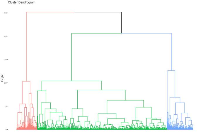
11.

grouped by latitude, longitude, capacity and price with AGNES and clusters=2

5. Conclusion

We have applied two agglomerative and partitional techniques to perform a study of the phenomenon of the collaborative economy within the tourism industry in Guanajuato City using real-world data. This data was obtained through Web Scraping to build a dataset of lodging hosts. This dataset contains the latitude, longitude capacity, and price of each available host.

Two clustering techniques were applied; K-means and AGNES with the number of groups determinate

Fig.

Fig.

Hosts

by the NbClustering tool. With this data, the best number of groups found by this analysis were 2 and 3. As future work can be made comparative between clusters using cluster statistics like hosts distance, the average price, the average rooms, the distance between clusters and other impact values to the tourism.

A CKN o WLEDGEMENTS

The authors want to Guanajuato University for the support provided for this research.

AUTHoRS

Juan Manuel Pérez-Rocha – Administrative Information Systems, DCEA-University of Guanajuato, Guanajuato, México, e-mail: jm.perezrocha@ugto.mx.

Jorge Alberto Soria-Alcaraz – Organizational Studies Department, DCEA-University of Guanajuato, Guanajuato, México, e-mail: jorge.soria@ugto.mx.

Rafael Guerrero-Rodríguez – Management and Business Management Department, DCEA-University of Guanajuato, Guanajuato, México, e-mail: r.guerrero@ugto.mx.

Omar Jair Purata-Sifuentes – Organizational Studies Department, DCEA-University of Guanajuato, Guanajuato, México, e-mail: opurata@yahoo.com.

Andrés Espinal – Organizational Studies Department, DCEA-University of Guanajuato, Guanajuato, México, e-mail: aespinal@ugto.mx.

Marco Aurelio Sotelo-Figueroa* – Organizational Studies Department, DCEA-University of Guanajuato, Guanajuato, México, e-mail: masotelo@ugto.mx.

* Corresponding author

R EFERENCES

[1] D. Dredge and S. Gyimóthy, “The collaborative economy and tourism: Critical perspectives, questionable claims and silenced voices”, Tourism Recreation Research, vol. 40, no. 3, 2015, 286–302, DOI: 10.1080/02508281.2015.1086076.

[2] D. Dredge and S. Gyimóthy, “Collaborative Economy and Tourism”, 2017, 1–12, DOI: 10.1007/978-3-319-51799-5_1.

[3] “The Collaborative Economy”. J. Owyang, C. Tran and C. Silva, https://www.slideshare.net/altimeter/the-collaborative-economy. Accessed on: 2020-05-28.

[4] D. Dredge and Sz. Gyimóthy, “The collaborative economy and tourism: Critical perspectives, questionable claims and silenced voices”, Tourism Recreation Research, vol. 40, no. 3, 2015, 286–302, DOI: 10.1080/02508281.2015.1086076.

[5] N. Gurran and P. Phibbs, “When Tourists Move In: How Should Urban Planners Respond to Airbnb?”, Journal of the American Planning Association, vol. 83, no. 1, 2017, 80–92, DOI: 10.1080/01944363.2016.1249011.

[6] Annual Activities Report; Secretaria de Turismo del Estado de Guanajuato, SECTUR. 2018. https://sectur.guanajuato.gob.mx. Accessed on: 2020-06-24.

[7] G. Zervas, D. Proserpio and J. W. Byers, “The Rise of the Sharing Economy: Estimating the Impact of Airbnb on the Hotel Industry”, Journal of Marketing Research, vol. 54, no. 5, 2017, 687–705, DOI: 10.1509/jmr.15.0204.

[8] D. Guttentag, S. Smith, L. Potwarka and M. Havitz, “Why Tourists Choose Airbnb: A Motivation-Based Segmentation Study”, Journal of Travel Research, vol. 57, no. 3, 2018, 342–359, DOI: 10.1177/0047287517696980.

[9] J. MacQueen, “Some methods for classification and analysis of multivariate observations”. In: Proceedings of the Fifth Berkeley Symposium on Mathematical Statistics and Probability, University of California Press, 1967, 281-297.

[10] A. K. Jain, “Data clustering: 50 years beyond K-means”, Pattern Recognition Letters, vol. 31, no. 8, 2010, 651–666, DOI: 10.1016/j.patrec.2009.09.011.

[11] W. H. E. Day and H. Edelsbrunner, “Efficient algorithms for agglomerative hierarchical clustering methods”, Journal of Classification, vol. 1, no. 1, 1984, 7–24, DOI: 10.1007/BF01890115.

[12] A. Bouguettaya, Q. Yu, X. Liu, X. Zhou and A. Song, “Efficient agglomerative hierarchical clustering”, Expert Systems with Applications, vol. 42, no. 5, 2015, 2785–2797.

[13] M. Garey, D. Johnson and H. Witsenhausen, “The complexity of the generalized Lloyd – Max problem (Corresp.)”, IEEE Transactions on Information Theory, vol. 28, no. 2, 1982, 255–256, DOI: 10.1109/TIT.1982.1056488.

[14] D. Guttentag, “Airbnb: disruptive innovation and the rise of an informal tourism accommodation sector”, Current Issues in Tourism, vol. 18, no. 12, 2015, 1192–1217, DOI: 10.1080/13683500.2013.827159.

[15] M. Charrad, N. Ghazzali, V. Boiteau and A. Niknafs, “NbClust: An R Package for Determining the Relevant Number of Clusters in a Data Set”, Journal of Statistical Software, vol. 61, no. 6, 2014, DOI: 10.18637/jss.v061.i06.

[16] D. Glez-Peña, A. Lourenço, H. López-Fernández, M. Reboiro-Jato and F. Fdez-Riverola, “Web scraping technologies in an API world”, Briefings in Bioinformatics, vol. 15, no. 5, 2014, 788–797, DOI: 10.1093/bib/bbt026.

[17] R. Guerrero Rodríguez, “Estudiando la relación del turismo con el desarrollo humano en destinos turísticos mexicanos”, Acta Universitaria, vol. 28, 2018, 01–06, DOI: 10.15174/au.2018.1886.

Research Trends on Fuzzy Logic Controller for Mobile Robot Navigation: A Scientometric Study

Submitted: 20th December 2019; accepted: 30th March 2020

Somiya Rani, Amita Jain, Oscar Castillo

DOI: 10.14313/JAMRIS/1-2020/11

Abstract: The present study shows the scientometric analysis of the publications on the fuzzy logic controller in autonomous mobile robot navigation during the period 2000 to 2018. The data is collected using Web of Science core collection database and analyzed at various levels such as Web of Science categories, publication years, document types, funding agencies, authors, research areas, countries or region, control terms, and organization to evaluate the research patterns. An extensive study is done to find the research trends in this area.

Keywords: Fuzzy Logic Controller, Autonomous Mobile Robot Navigation, type-2 Fuzzy logic, Optimized Fuzzy Controller

1. Introduction

The research in the field of robotics has shown great advancement in recent years. One of the latest applications in the robotics is autonomous navigation of robots when the surrounding environment is unstructured. Handling navigation and obstacle avoidance become very crucial in an unstructured environment. Fuzzy logic controller deemed to be appropriate for handling the navigation and obstacle related problems. Therefore, in this paper, the analysis is performed on the articles that have shown ways or methods to solve navigation and obstacle related problems in mobile robots using the fuzzy logic controller. This paper presents, a scientometric study on the fuzzy logic controller for autonomous mobile robot navigation. Web of Science is taken as the source to retrieve and analyze the data. A total of 307 documents which include 302 articles, 4 proceeding papers, and 1 book chapter are extracted from the period 2000-2018[1 to 307].

The scientometric study in this paper helps to understand various research patterns by answering the following research questions:

– Which research domain has the maximum number of publications in the field of fuzzy logic controller for mobile robot navigation?

– What is the growth rate of publication through the year 2000 to 2018?

– What are the various document types published in this area?

– Which funding agencies have the maximum number of research grants?

– Which author has the maximum number of publications in this field?

– Which research area has the maximum number of research papers in the field of the fuzzy logic controller for mobile robot navigations?

– Which country has contributed the most to this field?

– What are the various control terms associated with the fuzzy logic controller and mobile robot navigation?

– Which organization has the maximum number of publications?

In section 2, the methodology and material used for this study is discussed. Data interpretation and analysis of collected data at various levels such as Web of Science categories, publication years, document types, funding agencies, authors, research areas, countries or region, control terms, and organization are discussed in section 3. This study is concluded in section 4.

2. Methodology and Material

Web of Science is used as the data source to collect the data used in this study. It is a multidisciplinary database that supports 256 disciplines. The data is indexed in Science Citation Index Expanded (SCI-Expanded), Social Sciences Citation Index (SSCI) and Arts & Humanities Citation Index (A&HCI).

A total of 307 publications were retrieved for the queries listed in table 1. The table shows the source of data, Indexing, period, queries and total number of documents retrieved.

An analysis of collected data from the WoS using the searched queries as listed is performed at various levels such as WoS categories, publication years, document types, funding agencies, top authors, research areas, country or region, network plot of control terms and organization. A descriptive analysis of the data using various charts and graphs has been done in the next section.

Web of Science Science Citation Index-Expanded (SCI-E), SSCIA&HCI and ESCI.

2000-2018 “Fuzzy logic controller for robot navigation”, “Optimised fuzzy controller”, “type 1 OR type 2 Fuzzy logic for autonomous robot navigation”, “mobile robot motion planning”, “autonomous mobile robot navigation using soft computing”, “genetic algorithm-based path planning for mobile robots”, “autonomous robot* navigation* AND Fuzzy* logic controller*”, “autonomous robot navigation AND fuzzy controller AND fuzzy logic AND Mobile robot navigation”, “soft computing based mobile robot navigation”.

3. Data Interpretation and Analysis

Interpretation of research trends on publications in the field of fuzzy logic controller in the mobile robot navigation is performed in this section.

3.1.

Web of Science Categories

Web of Science core collection gives multiple options to search the queries such as basic search, author search, cited reference search and advanced search. In this section, the searched queries are analysed at WoS categories level which defines the domain of articles. A table for these categories with their respective record count is shown in table 2. The result shows that the maximum number of articles are published in computer science artificial intelligence category with record count of 139 articles. The second most frequent category is automation control systems with record count of 89 articles. A tree map corresponding to these categories is shown in figure 1.

1. Tree map for Web of Service categories with their respective record count

To observe the growth trends, we have used two scientometric measures i.e., Relative Growth Rate and Doubling Time. RGR and DT are used as a measure in growth analysis. The growth of any systm per unit time is referred to as Relative Growth Rate. RGR is calculated using the formula-

3.2. Publication Years

Figure 2 depicts the year-wise distribution of articles to show the number of articles published in a particular year. Most numbers of the articles are published in the year 2018 with a record count of 32 as opposed to the year 2000 with a record count of 11.

where,

ln(w1): Natural logarithm of the number of publications at time T1.

ln(w2): Natural logarithm of the number of publications at time T2.

T1: Initial time

T2: Final time

T2 – T1: Difference between initial time and final time. Because we are calculating RGR for successive years, the difference between initial time and final time is equal to 1. i.e.,

Thus,

Fig.

Tab. 2. Top 10 Web of Science Categories with record count

Tab. 1. List of queries used to collect data

RGR and DT of Publications

Doubling time (DT) is directly related to RGR. It is defined as the double-time of the existing growth rate. In [308], the author elaborated that the doubling time equates to the logarithm of 2 when the time required particular year to (4)

It can be observed from table 3 that the RGR is increased from the year 2000 (0.00) to 2018 (0.11). The highest RGR observed in the year 2001 and the lowest RGR is observed in the year 2015. On the other hand, the highest DT is observed in the year 2017 while the line graph is given to depict the relative growth rate and doubling time during the period of 2000 to 2018.

A table for top the 10 journals and their publication house with their respective count is also given in table 4. From this table, it can be observed that the maximum number of research articles are published in the journal “Robotics and Autonomous Systems” by ELSEVIER with a record count of 42. The second most frequent journal is “IEEE Transactions on Fuzzy Systems” by IEEE with a record count of 20.

RGR and DT of Publications

Tab. 3. RGR and DT of publications from year 2000 to 2018

Fig. 2. Year wise distribution of articles from year 2000 to 2018

Fig. 3. RGR and DT analysis of

Fig. 2. Year wise distribution of articles from year 2000 to 2018

Fig. 2.

4. Top 10

and publication house with record count

3.3. Document Types

The documents types selected for the analysis of the data are articles, proceeding papers, and book chapters. The maximum number of documents is of article type with a record count of 302. Only 4 proceeding papers and 1 book chapter is retrieved for the above-mentioned queries.

A table for document type with their respective record count is shown in table 5.

Tab. 5. Document types with respective record count

3.4. Funding Agencies

Various funding agencies have contributed to the publication of articles in order to carry out research in a specific domain. The name of the top 10 funding agencies that contributed to the field of the fuzzy logic controller for autonomous mobile robot navigation is listed in table 6. It can be observed from the table that the National Science Council of Taiwan with a record count of 13 has granted the maximum number of researches and the Ministry of Education and Science Spain has granted the minimum number of researches in this field. The top 10 countries corresponding to these funding agencies are mapped (in yellow color) on the world map as shown in Figure 4.

3.5 Authors

A list of top 15 authors who have contributed to field of the fuzzy logic controller for mobile robot navigation is given table 7.

From the table, it can be seen that the Parhi DR, Mbede JB, Lin CJ, Alsulaiman M, Pratihar DK, Algabri M, Chen CC, Faisal M, Juang CF, Mathkour H, Yang SX, Castillo O,

Gosine RG, Mann GKI, and Mohanty PK are the top 15 authors who have published their work in this field.

Fig. 4. World mapping of top 10 countries with maximum number of grants from funding agencies and maximum number of publications

Tab. 6. Table for top 10 funding agencies with record count

The research trend shows that the Parhi DR has contributed to this field with the maximum publications with count of 16.

Tab. 7. Record count of top 10 Authors

Tab. 8. Record Count of top 15 Research Areas

4 Alsulaiman M

5 Pratihar DK

6 Algabri M

8 Faisal M

15 Mohanty PK

A scattered plot is also given in figure 6 to visualize the number of papers published by the respective authors.

3.6 Research Areas

3.6. Research Areas

In this section, top 15 research areas in which the maximum number of publications has been published is discussed.

In this section, top 15 research areas in which the maximum number of publications has been published is discussed.

From the result, as shown in the table 8, it can be observed that the highest number of articles are published in the computer science area with a record count of 169 articles as opposed to educational research area with a record count of 2 articles. A pie chart and a radar chart for 5 and 10 major research areas is also shown in figure 5 and figure 7 respectively.

From the result, as shown in the table 8, it can be observed that the highest number of articles are published in the computer science area with a record count of 169 articles as opposed to educational research area with a record count of 2 articles. A pie chart and a radar chart for 5 and 10 major research areas is also shown in figure 5 and figure 7 respectively.

Tab. 9. Top 10 Countries with maximum number of publications

3.7 Country or Region

Top 10 countries across the globe have been visualized in figure 4 to depict the top 10 countries that have maximum number of publications in the field of fuzzy controller for mobile robot navigation. Table 9 shows top 10 countries contributed to this field.

Tab. 9. Top 10 Countries with maximum number of publications

3.7. Country or Region

Top 10 countries across the globe have been visualized in figure 4 to depict the top 10 countries that have maximum number of publications in the field of fuzzy controller for mobile robot navigation. Table 9 shows top 10 countries contributed to this field.

Tab. 10. Record count of publications of Top 10 organizations

Fig. 5. Top 5 Research Areas

Tab. 8. Record Count of top 15 Research

Fig. 5. Top 5

Authors

Authors

Fig. 6. Scattered plot for top 15 authors

Fig. 7. Radar chart for record count of top 10 Research

Fig. 8. Network Plot of

Fig. 6. Scattered plot for top 15 authors

Fig. 6. Scattered plot for top 15 authors

Fig. 7. Radar chart for record count of

Fig. 8. Network Plot of

Fig. 7. Radar chart for record count of top 10 Research Areas

Fig. 8. Network Plot of Control terms

3.8. Network Plot of Control Terms

Control terms refer to terms that have thought of interlinked with the study when an author does his research. We have taken 1260 control terms to visualize them using the network plot as shown in figure 9.

3.9. Organization

Various organizations have continuously contributed to this field in recent years among which the National Institute of Technology has the maximum number of publications with a record count of 10 articles followed by Huazhong University of Science and Technology with a record count of 9 articles. The name of top 10 organizations and the record count of number of papers published by authors from these organizations is given table 10 and a bar graph is also shown in figure 10.

Tab. 10. Record count of publications of Top 10 organizations

4. Conclusion

The present study gives the analytical description of publications in the field of the fuzzy logic controller for autonomous mobile robot navigation. In this paper, the publication history is explored. A total of 307 research papers are collected using the web of science database during the period 2000 to 2018. The assessment of the productivity of research in this area is performed at various levels such WoS categories, publication years, document types, funding agencies, top authors, research areas, country or region, network plot of control terms and organization, to get the deep insights in this field. From this study, it can be observed that the highest number of publications came in the year 2018. The most popular WoS category is computer science artificial intelligence with 139 publications in this field. The journal “Robotics and Autonomous Systems” has the highest number of publications. National Science Council of Taiwan is the most productive funding agency in this field that has shown the maximum number of research grants. Parhi DR is the most influential author and the National Institute of Technology has played a prominent role in the field of the fuzzy logic controller for autonomous mobile robot navigation.

In conclusion, the fuzzy logic controller for autonomous mobile robot navigation has played an important role in shaping academic research since its inception. Analysis of publications in a few more years to determine and explore the evolution and growth in this field can be a good future scope of this study.

AUTHORS

Somiya Rani – Ambedkar Institute of Advanced Communication Technologies and Research, East Delhi, India.

Fig. 9. Bar graph for top 10 organizations with number of publications

Amita Jain – Ambedkar Institute of Advanced Communication Technologies and Research, East Delhi, India.

Oscar Castillo* – Tijuana Institute of Technology, B.C., Tijuana, México, e-mail: ocastillo@tectijuana.mx.

*Corresponding author

Re F e R e NC e S

[1] H. A. Hagras, “A Hierarchical Type-2 Fuzzy Logic Control Architecture for Autonomous Mobile Robots”, IEEE Transactions on Fuzzy Systems, vol. 12, no. 4, 2004, 524–539, DOI: 10.1109/TFUZZ.2004.832538.

[2] R. Martínez, O. Castillo and L. T. Aguilar, “Optimization of interval type-2 fuzzy logic controllers for a perturbed autonomous wheeled mobile robot using genetic algorithms”, Information Sciences, vol. 179, no. 13, 2009, 2158–2174, DOI: 10.1016/j.ins.2008.12.028.

[3] M. A. P. Garcia, O. Montiel, O. Castillo, R. Sepúlveda and P. Melin, “Path planning for autonomous mobile robot navigation with ant colony optimization and fuzzy cost function evaluation”, Applied Soft Computing, vol. 9, no. 3, 2009, 1102–1110, DOI: 10.1016/j.asoc.2009.02.014.

[4] H. Seraji and A. Howard, “Behavior-based robot navigation on challenging terrain: A fuzzy logic approach”, IEEE Transactions on Robotics and Automation, vol. 18, no. 3, 2002, 308–321, DOI: 10.1109/TRA.2002.1019461.

[5] G. Antonelli, S. Chiaverini and G. Fusco, “A Fuzzy-Logic-Based Approach for Mobile Robot Path Tracking”, IEEE Transactions on Fuzzy Systems, vol. 15, no. 2, 2007, 211–221, DOI: 10.1109/TFUZZ.2006.879998.

[6] P. Rusu, E. M. Petriu, T. E. Whalen, A. Cornell and H. J. W. Spoelder, “Behavior-based neuro-fuzzy controller for mobile robot navigation”, IEEE Transactions on Instrumentation and Measurement, vol. 52, no. 4, 2003, 1335–1340, DOI: 10.1109/TIM.2003.816846.

[7] J. L. Martínez, A. Mandow, J. Morales, S. Pedraza and A. García-Cerezo, “Approximating Kinematics for Tracked Mobile Robots”, The International Journal of Robotics Research, vol. 24, no. 10, 2005, 867–878, DOI: 10.1177/0278364905058239.

[8] C.-F. Juang and Y.-C. Chang, “EvolutionaryGroup-Based Particle-Swarm-Optimized Fuzzy Controller With Application to Mobile-Robot Navigation in Unknown Environments”, IEEE Transactions on Fuzzy Systems, vol. 19, no. 2, 2011, 379–392, DOI: 10.1109/TFUZZ.2011.2104364.

[9] C. Ye, N. H. C. Yung and D.-W. Wang, “A fuzzy controller with supervised learning assisted

reinforcement learning algorithm for obstacle avoidance”, IEEE Transactions on Systems, Man and Cybernetics, Part B (Cybernetics), vol. 33, no. 1, 2003, 17–27, DOI: 10.1109/TSMCB.2003.808179.

[10] S. Sanchez-Solano, A. J. Cabrera, I. Baturone, F. J. Moreno-Velo and M. Brox, “FPGA Implementation of Embedded Fuzzy Controllers for Robotic Applications”, IEEE Transactions on Industrial Electronics, vol. 54, no. 4, 2007, 1937–1945, DOI: 10.1109/TIE.2007.898292.

[11] O. Montiel, U. Orozco-Rosas and R. Sepúlveda, “Path planning for mobile robots using Bacterial Potential Field for avoiding static and dynamic obstacles”, Expert Systems with Applications, vol. 42, no. 12, 2015, 5177–5191, DOI: 10.1016/j.eswa.2015.02.033.

[12] W. Gueaieb and M. S. Miah, “An Intelligent Mobile Robot Navigation Technique Using RFID Technology”, IEEE Transactions on Instrumentation and Measurement, vol. 57, no. 9, 2008, 1908–1917, DOI: 10.1109/TIM.2008.919902.

[13] F. Abdessemed, K. Benmahammed and E. Monacelli, “A fuzzy-based reactive controller for a non-holonomic mobile robot”, Robotics and Autonomous Systems, vol. 47, no. 1, 2004, 31–46, DOI: 10.1016/j.robot.2004.02.006.

[14] N. C. Tsourveloudis, K. P. Valavanis and T. Hebert, “Autonomous vehicle navigation utilizing electrostatic potential fields and fuzzy logic”, IEEE Transactions on Robotics and Automation, vol. 17, no. 4, 2001, 490–497, DOI: 10.1109/70.954761.

[15] H. Maaref and C. Barret, “Sensor-based navigation of a mobile robot in an indoor environment”, Robotics and Autonomous Systems, vol. 38, no. 1, 2002, 2020–01-18, DOI: 10.1016/S0921-8890(01)00165-8.

[16] S. K. Pradhan, D. R. Parhi and A. K. Panda, “Fuzzy logic techniques for navigation of several mobile robots”, Applied Soft Computing, vol. 9, no. 1, 2009, 290–304, DOI: 10.1016/j.asoc.2008.04.008.

[17] M. Wang and J. N. K. Liu, “Fuzzy logic-based real-time robot navigation in unknown environment with dead ends”, Robotics and Autonomous Systems, vol. 56, no. 7, 2008, 625–643, DOI: 10.1016/j.robot.2007.10.002.

[18] C.-H. Hsu and C.-F. Juang, “Evolutionary Robot Wall-Following Control Using Type-2 Fuzzy Controller With Species-DE-Activated Continuous ACO”, IEEE Transactions on Fuzzy Systems, vol. 21, no. 1, 2013, 100–112, DOI: 10.1109/TFUZZ.2012.2202665.

[19] S.-M. Lee, K.-Y. Kwon and J. Joh, “A fuzzy logic for autonomous navigation of marine vehicles satisfying COLREG guidelines”, International Journal of Control Automation and Systems, vol. 2, no. 2, 2004, 171-181.

[20] X. Yang, M. Moallem and R. V. Patel, “A Layered Goal-Oriented Fuzzy Motion Planning Strategy for Mobile Robot Navigation”, IEEE Transactions on Systems, Man and Cybernetics, Part B (Cybernetics), vol. 35, no. 6, 2005, 1214–1224, DOI: 10.1109/TSMCB.2005.850177.

[21] E. Aguirre and A. González, “Fuzzy behaviors for mobile robot navigation: design, coordination and fusion”, International Journal of Approximate Reasoning, vol. 25, no. 3, 2000, 255–289, DOI: 10.1016/S0888-613X(00)00056-6.

[22] C.-J. Kim and D. Chwa, “Obstacle Avoidance Method for Wheeled Mobile Robots Using Interval Type-2 Fuzzy Neural Network”, IEEE Transactions on Fuzzy Systems, vol. 23, no. 3, 2015, 677–687, DOI: 10.1109/TFUZZ.2014.2321771.

[23] K. R. S. Kodagoda, W. S. Wijesoma and E. K. Teoh, “Fuzzy speed and steering control of an AGV”, IEEE Transactions on Control Systems Technology, vol. 10, no. 1, 2002, 112–120, DOI: 10.1109/87.974344.

[24] S. Kim and J.-H. Kim, “Adaptive fuzzy-networkbased C-measure map-matching algorithm for car navigation system”, IEEE Transactions on Industrial Electronics, vol. 48, no. 2, 2001, 432–441, DOI: 10.1109/41.915423.

[25] N. B. Hui, V. Mahendar and D. K. Pratihar, “Timeoptimal, collision-free navigation of a car-like mobile robot using neuro-fuzzy approaches”, Fuzzy Sets and Systems, vol. 157, no. 16, 2006, 2171–2204, DOI: 10.1016/j.fss.2006.04.004.

[26] M. F. Selekwa, D. D. Dunlap, D. Shi and E. G. Collins, “Robot navigation in very cluttered environments by preference-based fuzzy behaviors”, Robotics and Autonomous Systems, vol. 56, no. 3, 2008, 231–246, DOI: 10.1016/j.robot.2007.07.006.

[27] H. Mousazadeh, “A technical review on navigation systems of agricultural autonomous off-road vehicles”, Journal of Terramechanics, vol. 50, no. 3, 2013, 211–232, DOI: 10.1016/j.jterra.2013.03.004.

[28] M. Mucientes and J. Casillas, “Quick Design of Fuzzy Controllers With Good Interpretability in Mobile Robotics”, IEEE Transactions on Fuzzy Systems, vol. 15, no. 4, 2007, 636–651, DOI: 10.1109/TFUZZ.2006.889889.

[29] J. L. Martínez, J. González, J. Morales, A. Mandow and A. J. García-Cerezo, “Mobile robot motion estimation by 2D scan matching with genetic and iterative closest point algorithms”, Journal of Field Robotics, vol. 23, no. 1, 2006, 21–34, DOI: 10.1002/rob.20104.

[30] J. Xue, L. Zhang and T. E. Grift, “Variable field-ofview machine vision based row guidance of an

agricultural robot”, Computers and Electronics in Agriculture, vol. 84, 2012, 85–91, DOI: 10.1016/j.compag.2012.02.009.

[31] R.-J. Wai and Y.-W. Lin, “Adaptive Moving-Target Tracking Control of a Vision-Based Mobile Robot via a Dynamic Petri Recurrent Fuzzy Neural Network”, IEEE Transactions on Fuzzy Systems, vol. 21, no. 4, 2013, 688–701, DOI: 10.1109/TFUZZ.2012.2227974.

[32] F. Cupertino, V. Giordano, D. Naso and L. Delfine, “Fuzzy control of a mobile robot”, IEEE Robotics & Automation Magazine, vol. 13, no. 4, 2006, 74–81, DOI: 10.1109/MRA.2006.250563.

[33] L. Moreno, J. M. Armingol, S. Garrido, A. de la Escalera and M. A. Salichs, “A Genetic Algorithm for Mobile Robot Localization Using Ultrasonic Sensors”, Journal of Intelligent and Robotic Systems, vol. 34, no. 2, 2002, 135–154, DOI: 10.1023/A:1015664517164.

[34] F. Arambula Cosío and M. A. Padilla Castañeda, “Autonomous robot navigation using adaptive potential fields”, Mathematical and Computer Modelling, vol. 40, no. 9-10, 2004, 1141–1156, DOI: 10.1016/j.mcm.2004.05.001.

[35] R. Kala, A. Shukla and R. Tiwari, “Fusion of probabilistic A* algorithm and fuzzy inference system for robotic path planning”, Artificial Intelligence Review, vol. 33, no. 4, 2010, 307–327, DOI: 10.1007/s10462-010-9157-y.

[36] E. Kayacan, E. Kayacan, H. Ramon, O. Kaynak and W. Saeys, “Towards Agrobots: Trajectory Control of an Autonomous Tractor Using Type2 Fuzzy Logic Controllers”, IEEE/ASME Transactions on Mechatronics, vol. 20, no. 1, 2015, 287–298, DOI: 10.1109/TMECH.2013.2291874.

[37] C.-H. Hsu and C.-F. Juang, “Multi-Objective Continuous-Ant-Colony-Optimized FC for Robot Wall-Following Control”, IEEE Computational Intelligence Magazine, vol. 8, no. 3, 2013, 28–40, DOI: 10.1109/MCI.2013.2264233.

[38] D. R. Parhi, “Navigation of Mobile Robots Using a Fuzzy Logic Controller”, Journal of Intelligent and Robotic Systems, vol. 42, no. 3, 2005, 253–273, DOI: 10.1007/s10846-004-7195-x.

[39] M. Faisal, R. Hedjar, M. Al Sulaiman and K. AlMutib, “Fuzzy Logic Navigation and Obstacle Avoidance by a Mobile Robot in an Unknown Dynamic Environment”, International Journal of Advanced Robotic Systems, vol. 10, no. 1, 2013, DOI: 10.5772/54427.

[40] C.-C. Tsai, H.-C. Huang and S.-C. Lin, “FPGABased Parallel DNA Algorithm for Optimal Configurations of an Omnidirectional Mobile Service Robot Performing Fire Extinguishment”, IEEE Transactions on Industrial Electronics, vol. 58, no. 3, 2011, 1016–1026, DOI: 10.1109/TIE.2010.2048291.

[41] H.-H. Lin, C.-C. Tsai and J.-C. Hsu, “Ultrasonic Localization and Pose Tracking of an Autonomous Mobile Robot via Fuzzy Adaptive Extended Information Filtering”, IEEE Transactions on Instrumentation and Measurement, vol. 57, no. 9, 2008, 2024–2034, DOI: 10.1109/TIM.2008.919020.

[42] H. Li and S. X. Yang, “A behavior-based mobile robot with a visual landmark-recognition system”, IEEE/ASME Transactions on Mechatronics, vol. 8, no. 3, 2003, 390–400, DOI: 10.1109/TMECH.2003.816818.

[43] J. B. Mbede, X.-H. Huang and M. Wang, “Robust neuro-fuzzy sensor-based motion control among dynamic obstacles for robot manipulators”, IEEE Transactions on Fuzzy Systems, vol. 11, no. 2, 2003, 249–261, DOI: 10.1109/TFUZZ.2003.809906.

[44] T. Haferlach, J. Wessnitzer, M. Mangan and B. Webb, “Evolving a Neural Model of Insect Path Integration”, Adaptive Behavior, vol. 15, no. 3, 2007, 273–287, DOI: 10.1177/1059712307082080.

[45] R. Huq, G. K. I. Mann and R. G. Gosine, “Behaviormodulation technique in mobile robotics using fuzzy discrete event system”, IEEE Transactions on Robotics, vol. 22, no. 5, 2006, 903–916, DOI: 10.1109/TRO.2006.878937.

[46] H. Mehrjerdi, M. Saad and J. Ghommam, “Hierarchical Fuzzy Cooperative Control and Path Following for a Team of Mobile Robots”, IEEE/ ASME Transactions on Mechatronics, vol. 16, no. 5, 2011, 907–917, DOI: 10.1109/TMECH.2010.2054101.

[47] J. Velagic, B. Lacevic and B. Perunicic, “A 3-level autonomous mobile robot navigation system designed by using reasoning/search approaches”, Robotics and Autonomous Systems, vol. 54, no. 12, 2006, 989–1004, DOI: 10.1016/j.robot.2006.05.006.

[48] H. Hagras, V. Callaghan and M. Colley, “Learning and adaptation of an intelligent mobile robot navigator operating in unstructured environment based on a novel online Fuzzy–Genetic system”, Fuzzy Sets and Systems, vol. 141, no. 1, 2004, 107–160, DOI: 10.1016/S0165-0114(03)00116-7.

[49] D. K. Pratihar, K. Deb and A. Ghosh, “Optimal path and gait generations simultaneously of a six-legged robot using a GA-fuzzy approach”, Robotics and Autonomous Systems, vol. 41, no. 1, 2002, 2020–01-20, DOI: 10.1016/S0921-8890(02)00273-7.

[50] J. K. Pothal and D. R. Parhi, “Navigation of multiple mobile robots in a highly clutter terrains using adaptive neuro-fuzzy inference system”, Robotics and Autonomous Systems, vol. 72, 2015, 48–58, DOI: 10.1016/j.robot.2015.04.007.

[51] D. Gu and H. Hu, “Using Fuzzy Logic to Design Separation Function in Flocking Algorithms”,

IEEE Transactions on Fuzzy Systems, vol. 16, no. 4, 2008, 826–838, DOI: 10.1109/TFUZZ.2008.917289.

[52] A. Bakdi, A. Hentout, H. Boutami, A. Maoudj, O. Hachour and B. Bouzouia, “Optimal path planning and execution for mobile robots using genetic algorithm and adaptive fuzzy-logic control”, Robotics and Autonomous Systems, vol. 89, 2017, 95–109, DOI: 10.1016/j.robot.2016.12.008.

[53] K. Samsudin, F. A. Ahmad and S. Mashohor, “A highly interpretable fuzzy rule base using ordinal structure for obstacle avoidance of mobile robot”, Applied Soft Computing, vol. 11, no. 2, 2011, 1631–1637, DOI: 10.1016/j.asoc.2010.05.002.

[54] S. X. Yang, H. Li, M. Q. H. Meng and P. X. Liu, “An Embedded Fuzzy Controller for a BehaviorBased Mobile Robot With Guaranteed Performance”, IEEE Transactions on Fuzzy Systems, vol. 12, no. 4, 2004, 436–446, DOI: 10.1109/TFUZZ.2004.832524.

[55] M. Akbarzadeh, K. Kumbla, E. Tunstel and M. Jamshidi, “Soft computing for autonomous robotic systems”, Computers & Electrical Engineering, vol. 26, no. 1, 2000, 5–32, DOI: 10.1016/S0045-7906(99)00027-0.

[56] H. Miao and Y.-C. Tian, “Dynamic robot path planning using an enhanced simulated annealing approach”, Applied Mathematics and Computation, vol. 222, 2013, 420–437, DOI: 10.1016/j.amc.2013.07.022.

[57] R. Chatterjee and F. Matsuno, “Use of single side reflex for autonomous navigation of mobile robots in unknown environments”, Robotics and Autonomous Systems, vol. 35, no. 2, 2001, 77–96, DOI: 10.1016/S0921-8890(00)00124-X.

[58] K. Althoefer, B. Krekelberg, D. Husmeier and L. Seneviratne, “Reinforcement learning in a rule-based navigator for robotic manipulators”, Neurocomputing, vol. 37, 2001, 51–70, DOI: 10.1016/S0925-2312(00)00307-6.

[59] J. C. Mohanta, D. R. Parhi and S. K. Patel, “Path planning strategy for autonomous mobile robot navigation using Petri-GA optimisation”, Computers & Electrical Engineering, vol. 37, no. 6, 2011, 1058–1070, DOI: 10.1016/j.compeleceng.2011.07.007.

[60] J. Mbede, P. Ele, C. Mvehabia, Y. Toure, V. Graefe and S. Ma, “Intelligent mobile manipulator navigation using adaptive neuro-fuzzy systems”, Information Sciences, vol. 171, no. 4, 2005, 447–474, DOI: 10.1016/j.ins.2004.09.014.

[61] J. Z. Sasiadek and Q. Wang, “Low cost automation using INS/GPS data fusion for accurate positioning”, Robotica, vol. 21, no. 3, 2003, 255–260, DOI: 10.1017/S0263574702004757.

[62] M. Al-Khatib and J. J. Saade,“An efficient datadriven fuzzy approach to the motion planning

problem of a mobile robot”, Fuzzy Sets and Systems, vol. 134, no. 1, 2003, 65–82, DOI: 10.1016/S0165-0114(02)00230-0.

[63] F. Hoffmann, D. Schauten and S. Holemann, “Incremental Evolutionary Design of TSK Fuzzy Controllers”, IEEE Transactions on Fuzzy Systems, vol. 15, no. 4, 2007, 563–577, DOI: 10.1109/TFUZZ.2007.900905.

[64] V. Kanakakis, K. P. Valavanis and N. C. Tsourveloudis, “Fuzzy-Logic Based Navigation of Underwater Vehicles”, Journal of Intelligent and Robotic Systems, vol. 40, no. 1, 2004, 45–88, DOI: 10.1023/B:JINT.0000034340.87020.05.

[65] M. Algabri, H. Mathkour, H. Ramdane and M. Alsulaiman, “Comparative study of soft computing techniques for mobile robot navigation in an unknown environment”, Computers in Human Behavior, vol. 50, 2015, 42–56, DOI: 10.1016/j.chb.2015.03.062.

[66] K. Das Sharma, A. Chatterjee and A. Rakshit, “A PSO–Lyapunov Hybrid Stable Adaptive Fuzzy Tracking Control Approach for VisionBased Robot Navigation”, IEEE Transactions on Instrumentation and Measurement, vol. 61, no. 7, 2012, 1908–1914, DOI: 10.1109/TIM.2012.2182868.

[67] K. Madhava Krishna and P. K. Kalra, “Detection, Tracking and Avoidance of Multiple Dynamic Objects”, Journal of Intelligent and Robotic Systems, vol. 33, no. 4, 2002, 371–408, DOI: 10.1023/A:1015508906105.

[68] J. Rosenblatt, S. Williams and H. DurrantWhyte, “A behavior-based architecture for autonomous underwater exploration”, Information Sciences, vol. 145, no. 2020-01-02, 2002, 69–87, DOI: 10.1016/S0020-0255(02)00224-4.

[69] J. B. Mbede, X. Huang and M. Wang, “Fuzzy motion planning among dynamic obstacles using artificial potential fields for robot manipulators”, Robotics and Autonomous Systems, vol. 32, no. 1, 2000, 61–72, DOI: 10.1016/S0921-8890(00)00073-7.

[70] H.-M. Feng, C.-Y. Chen and J.-H. Horng, “Intelligent omni-directional vision-based mobile robot fuzzy systems design and implementation”, Expert Systems with Applications, vol. 37, no. 5, 2010, 4009–4019, DOI: 10.1016/j.eswa.2009.11.030.

[71] E. A. Merchan-Cruz and A. S. Morris, “FuzzyGA-based trajectory planner for robot manipulators sharing a common workspace”, IEEE Transactions on Robotics, vol. 22, no. 4, 2006, 613–624, DOI: 10.1109/TRO.2006.878789.

[72] X.-D. Chen, K. Watanabe, K. Kiguchi and K. Izumi, “An ART-based fuzzy controller for the adaptive navigation of a quadruped robot”, IEEE/ASME Transactions on Mechatronics, vol. 7, no. 3, 2002, 318–328, DOI: 10.1109/TMECH.2002.802722.

[73] C.-F. Juang, T.-L. Jeng and Y.-C. Chang, “An Interpretable Fuzzy System Learned Through Online Rule Generation and Multiobjective ACO With a Mobile Robot Control Application”, IEEE Transactions on Cybernetics, vol. 46, no. 12, 2016, 2706–2718, DOI: 10.1109/TCYB.2015.2486779.

[74] A. H. Karami and M. Hasanzadeh, “An adaptive genetic algorithm for robot motion planning in 2D complex environments”, Computers & Electrical Engineering, vol. 43, 2015, 317–329, DOI: 10.1016/j.compeleceng.2014.12.014.

[75] N. B. Hui and D. K. Pratihar, “A comparative study on some navigation schemes of a real robot tackling moving obstacles”, Robotics and Computer-Integrated Manufacturing, vol. 25, no. 4-5, 2009, 810–828, DOI: 10.1016/j.rcim.2008.12.003.

[76] S. Nefti, M. Oussalah, K. Djouani and J. Pontnau, “Intelligent Adaptive Mobile Robot Navigation”, Journal of Intelligent and Robotic Systems, vol. 30, no. 4, 2001, 311–329, DOI: 10.1023/A:1011190306492.

[77] P. K. Mohanty and D. R. Parhi, “A New Intelligent Motion Planning for Mobile Robot Navigation using Multiple Adaptive Neuro-Fuzzy Inference System”, Applied Mathematics & Information Sciences, vol. 8, no. 5, 2014, 2527–2535, DOI: 10.12785/amis/080551.

[78] D. R. Parhi and J. C. Mohanta, “Navigational control of several mobile robotic agents using Petri-potential-fuzzy hybrid controller”, Applied Soft Computing, vol. 11, no. 4, 2011, 3546–3557, DOI: 10.1016/j.asoc.2011.01.027.

[79] E. Tunstel, M. A. A. de Oliveira and S. Berman, “Fuzzy behavior hierarchies for multi-robot control”, International Journal of Intelligent Systems, vol. 17, no. 5, 2002, 449–470, DOI: 10.1002/int.10032.

[80] N. Kubota, T. Morioka, F. Kojima and T. Fukuda, “Learning of mobile robots using perceptionbased genetic algorithm”, Measurement, vol. 29, no. 3, 2001, 237–248, DOI: 10.1016/S0263-2241(00)00044-0.

[81] D. Dong, C. Chen, C. Zhang and Z. Chen, “Quantum robot: structure, algorithms and applications”, Robotica, vol. 24, no. 4, 2006, 513–521, DOI: 10.1017/S0263574705002596.

[82] H. Yavuz and A. Bradshaw, “A New Conceptual Approach to the Design of Hybrid Control Architecture for Autonomous Mobile Robots”, Journal of Intelligent and Robotic Systems, vol. 34, no. 1, 2002, 2020–01-26, DOI: 10.1023/A:1015522622034.

[83] H. Maaref and C. Barret, “Sensor-based fuzzy navigation of an autonomous mobile robot in an indoor environment”, Control Engineering Practice, vol. 8, no. 7, 2000, 757–768, DOI: 10.1016/S0967-0661(99)00200-2.

[84] Y. Li, G. Wang, H. Chen, L. Shi and L. Qin, “An Ant Colony Optimization Based Dimension Reduction Method for High-Dimensional Datasets”, Journal of Bionic Engineering, vol. 10, no. 2, 2013, 231–241, DOI: 10.1016/S1672-6529(13)60219-X.

[85] T. Yang and V. Aitken, “Evidential Mapping for Mobile Robots With Range Sensors”, IEEE Transactions on Instrumentation and Measurement, vol. 55, no. 4, 2006, 1422–1429, DOI: 10.1109/TIM.2006.876399.

[86] P. K. Mohanty and D. R. Parhi, “A new hybrid optimization algorithm for multiple mobile robots navigation based on the CS-ANFIS approach”, Memetic Computing, vol. 7, no. 4, 2015, 255–273, DOI: 10.1007/s12293-015-0160-3.

[87] G. K. Venayagamoorthy, L. L. Grant and S. Doctor, “Collective robotic search using hybrid techniques: Fuzzy logic and swarm intelligence inspired by nature”, Engineering Applications of Artificial Intelligence, vol. 22, no. 3, 2009, 431–441, DOI: 10.1016/j.engappai.2008.10.002.

[88] E. Aguirre and A. González, “A Fuzzy Perceptual Model for Ultrasound Sensors Applied to Intelligent Navigation of Mobile Robots”, Applied Intelligence, vol. 19, no. 3, 2003, 171–187, DOI: 10.1023/A:1026057906312.

[89] A. Pandey and D. R. Parhi, “Optimum path planning of mobile robot in unknown static and dynamic environments using Fuzzy-Wind Driven Optimization algorithm”, Defence Technology, vol. 13, no. 1, 2017, 47–58, DOI: 10.1016/j.dt.2017.01.001.

[90] M. S. Masmoudi, N. Krichen, M. Masmoudi and N. Derbel, “Fuzzy logic controllers design for omnidirectional mobile robot navigation”, Applied Soft Computing, vol. 49, 2016, 901–919, DOI: 10.1016/j.asoc.2016.08.057.

[91] S.-Y. Lee and H.-W. Yang, “Navigation of automated guided vehicles using magnet spot guidance method”, Robotics and ComputerIntegrated Manufacturing, vol. 28, no. 3, 2012, 425–436, DOI: 10.1016/j.rcim.2011.11.005.

[92] A. Jayasiri, G. K. I. Mann and R. G. Gosine, “Behavior Coordination of Mobile Robotics Using Supervisory Control of Fuzzy Discrete Event Systems”, IEEE Transactions on Systems, Man, and Cybernetics, Part B (Cybernetics), vol. 41, no. 5, 2011, 1224–1238, DOI: 10.1109/TSMCB.2011.2119311.

[93] A. M. Martinez and J. Vitria, “Clustering in image space for place recognition and visual annotations for human-robot interaction”, IEEE Transactions on Systems, Man and Cybernetics, Part B (Cybernetics), vol. 31, no. 5, 2001, 669–682, DOI: 10.1109/3477.956029.

[94] W. L. Xu, “A virtual target approach for resolving the limit cycle problem in navigation of a fuzzy behaviour-based mobile robot”, Ro-

botics and Autonomous Systems, vol. 30, no. 4, 2000, 315–324, DOI: 10.1016/S0921-8890(99)00099-8.

[95] C.-F. Juang, M.-G. Lai and W.-T. Zeng, “Evolutionary Fuzzy Control and Navigation for Two Wheeled Robots Cooperatively Carrying an Object in Unknown Environments”, IEEE Transactions on Cybernetics, vol. 45, no. 9, 2015, 1731–1743, DOI: 10.1109/TCYB.2014.2359966.

[96] F. Janabi-Sharifi and I. Hassanzadeh, “Experimental Analysis of Mobile-Robot Teleoperation via Shared Impedance Control”, IEEE Transactions on Systems, Man, and Cybernetics, Part B (Cybernetics), vol. 41, no. 2, 2011, 591–606, DOI: 10.1109/TSMCB.2010.2073702.

[97] S. Nefti, M. Oussalah and U. Kaymak, “A New Fuzzy Set Merging Technique Using InclusionBased Fuzzy Clustering”, IEEE Transactions on Fuzzy Systems, vol. 16, no. 1, 2008, 145–161, DOI: 10.1109/TFUZZ.2007.902011.

[98] K.-Y. Tu and J. Baltes, “Fuzzy potential energy for a map approach to robot navigation”, Robotics and Autonomous Systems, vol. 54, no. 7, 2006, 574–589, DOI: 10.1016/j.robot.2006.04.001.

[99] J. Huang, M. Ri, D. Wu and S. Ri, “Interval Type-2 Fuzzy Logic Modeling and Control of a Mobile Two-Wheeled Inverted Pendulum”, IEEE Transactions on Fuzzy Systems, vol. 26, no. 4, 2018, 2030–2038, DOI: 10.1109/TFUZZ.2017.2760283.

[100] U. Orozco-Rosas, O. Montiel and R. Sepúlveda, “Pseudo-Bacterial Potential Field Based Path Planner for Autonomous Mobile Robot Navigation”, International Journal of Advanced Robotic Systems, vol. 12, no. 7, 2015, DOI: 10.5772/60715.

[101] J. M. Alonso, M. Ocaña, N. Hernandez, F. Herranz, A. Llamazares, M. A. Sotelo, L. M. Bergasa and L. Magdalena, “Enhanced WiFi localization system based on Soft Computing techniques to deal with small-scale variations in wireless sensors”, Applied Soft Computing, vol. 11, no. 8, 2011, 4677–4691, DOI: 10.1016/j.asoc.2011.07.015.

[102] Y.-D. Hong, Y.-H. Kim, J.-H. Han, J.-K. Yoo and J.-H. Kim, “Evolutionary Multiobjective Footstep Planning for Humanoid Robots”, IEEE Transactions on Systems, Man, and Cybernetics, Part C (Applications and Reviews), vol. 41, no. 4, 2011, 520–532, DOI: 10.1109/TSMCC.2010.2063700.

[103] R. Kala, A. Shukla and R. Tiwari, “Robotic path planning using evolutionary momentumbased exploration”, Journal of Experimental & Theoretical Artificial Intelligence, vol. 23, no. 4, 2011, 469–495, DOI: 10.1080/0952813X.2010.490963.

[104] H. Boubertakh, M. Tadjine and P. Glorennec, “A new mobile robot navigation method using fuzzy logic and a modified Q-learning algo-

rithm”, Journal of Intelligent & Fuzzy Systems, vol. 21, no. 1-2, 2010, 113–119, DOI: 10.3233/IFS-2010-0440.

[105] M. Mucientes, R. Iglesias, C. V. Regueiro, A. Bugarin, P. Carinena and S. Barro, “Fuzzy temporal rules for mobile robot guidance in dynamic environments”, IEEE Transactions on Systems, Man and Cybernetics, Part C (Applications and Reviews), vol. 31, no. 3, 2001, 391–398, DOI: 10.1109/5326.971667.

[106] O. Montiel-Ross, R. Sepúlveda, O. Castillo and P. Melin, “Ant colony test center for planning autonomous mobile robot navigation”, Computer Applications in Engineering Education, vol. 21, no. 2, 2013, 214–229, DOI: 10.1002/cae.20463.

[107] S. Hong and S. Park, “Minimal-Drift Heading Measurement using a MEMS Gyro for Indoor Mobile Robots”, Sensors, vol. 8, no. 11, 2008, 7287–7299, DOI: 10.3390/s8117287.

[108] G.-C. Luh and W.-W. Liu, “Motion planning for mobile robots in dynamic environments using a potential field immune network”, Proceedings of the Institution of Mechanical Engineers, Part I: Journal of Systems and Control Engineering, vol. 221, no. 7, 2007, 1033–1045, DOI: 10.1243/09596518JSCE400.

[109] M. Mitić and Z. Miljković, “Bio-inspired approach to learning robot motion trajectories and visual control commands”, Expert Systems with Applications, vol. 42, no. 5, 2015, 2624–2637, DOI: 10.1016/j.eswa.2014.10.053.

[110] R. Huq, G. K. I. Mann and R. G. Gosine, “Distributed fuzzy discrete event system for robotic sensory information processing”, Expert Systems, vol. 23, no. 5, 2006, 273–289, DOI: 10.1111/j.1468-0394.2006.00409.x.

[111] P.-S. Tsai, L.-S. Wang and F.-R. Chang, “Modeling and hierarchical tracking control of triwheeled mobile robots”, IEEE Transactions on Robotics, vol. 22, no. 5, 2006, 1055–1062, DOI: 10.1109/TRO.2006.878964.

[112] B. Sun, D. Zhu, L. Jiang and S. X. Yang, “A novel fuzzy control algorithm for three-dimensional AUV path planning based on sonar model”, Journal of Intelligent & Fuzzy Systems, vol. 26, no. 6, 2014, 2913–2926, DOI: 10.3233/IFS-130957.

[113] L. Khriji, F. Touati, K. Benhmed and A. Al-Yahmedi, “Mobile Robot Navigation Based on Q-Learning Technique”, International Journal of Advanced Robotic Systems, vol. 8, no. 1, 2011, DOI: 10.5772/10528.

[114] H. M. Barberá and A. G. Skarmeta, “A framework for defining and learning fuzzy behaviors for autonomous mobile robots”, International Journal of Intelligent Systems, vol. 17, no. 1, 2002, DOI: 10.1002/int.1000.

[115] J. Bengochea-Guevara, J. Conesa-Muñoz, D. Andújar and A. Ribeiro, “Merge Fuzzy Visual Servoing and GPS-Based Planning to Obtain a Proper Navigation Behavior for a Small CropInspection Robot”, Sensors, vol. 16, no. 3, 2016, DOI: 10.3390/s16030276.

[116] C.-H. Kuo, H.-C. Chou and S.-Y. Tasi, “Pneumatic Sensor: A Complete Coverage Improvement Approach for Robotic Cleaners”, IEEE Transactions on Instrumentation and Measurement, vol. 60, no. 4, 2011, 1237–1256, DOI: 10.1109/TIM.2010.2101312.

[117] J. Kim, Y.-G. Kim and J. An, “A Fuzzy Obstacle Avoidance Controller Using a Lookup-Table Sharing Method and Its Applications for Mobile Robots”, International Journal of Advanced Robotic Systems, vol. 8, no. 5, 2011, DOI: 10.5772/45700.

[118] D. Herrero-Pérez, H. Martínez-Barberá, K. LeBlanc and A. Saffiotti, “Fuzzy uncertainty modeling for grid based localization of mobile robots”, International Journal of Approximate Reasoning, vol. 51, no. 8, 2010, 912–932, DOI: 10.1016/j.ijar.2010.06.001.

[119] M. Yahyaei, J. E. Jam and R. Hosnavi, “Controlling the navigation of automatic guided vehicle (AGV) using integrated fuzzy logic controller with programmable logic controller (IFLPLC)—stage 1”, The International Journal of Advanced Manufacturing Technology, vol. 47, no. 5-8, 2010, 795–807, DOI: 10.1007/s00170-009-2017-8.

[120] R. Abiyev, D. Ibrahim and B. Erin, “EDURobot: an educational computer simulation program for navigation of mobile robots in the presence of obstacles”, The International journal of engineering education, vol. 26, no. 1, 2010, 18–29.

[121] D. R. Parhi and M. K. Singh, “Intelligent fuzzy interface technique for the control of an autonomous mobile robot”, Proceedings of the Institution of Mechanical Engineers, Part C: Journal of Mechanical Engineering Science, vol. 222, no. 11, 2008, 2281–2292, DOI: 10.1243/09544062JMES955.

[122] R. Munoz-Salinas, E. Aguirre, O. Cordon and M. Garcia-Silvente, “Automatic Tuning of a Fuzzy Visual System Using Evolutionary Algorithms: Single-Objective Versus Multiobjective Approaches”, IEEE Transactions on Fuzzy Systems, vol. 16, no. 2, 2008, 485–501, DOI: 10.1109/TFUZZ.2006.889954.

[123] R. Muñoz-Salinas, E. Aguirre and M. García-Silvente, “Detection of doors using a genetic visual fuzzy system for mobile robots”, Autonomous Robots, vol. 21, no. 2, 2006, 123–141, DOI: 10.1007/s10514-006-7847-8.

[124] M. Mucientes, D. L. Moreno, A. Bugarín and S. Barro, “Evolutionary learning of a fuzzy controller for wall-following behavior in mobile robotics”, Soft Computing, vol. 10, no. 10, 2006, 881–889, DOI: 10.1007/s00500-005-0014-x.

[125] C. Ye and D. Wang, “A Novel Navigation Method for Autonomous Mobile Vehicles”, Journal of Intelligent and Robotic Systems, vol. 32, no. 4, 2001, 361–388, DOI: 10.1023/A:1014224418743.

[126] F. Fathinezhad, V. Derhami and M. Rezaeian, “Supervised fuzzy reinforcement learning for robot navigation”, Applied Soft Computing , vol. 40, 2016, 33–41, DOI: 10.1016/j.asoc.2015.11.030.

[127] H. Omrane, M. S. Masmoudi and M. Masmoudi, “Fuzzy Logic Based Control for Autonomous Mobile Robot Navigation”, Computational Intelligence and Neuroscience, 2016, 1–10, DOI: 10.1155/2016/9548482.

[128] D. Gu and H. Hu, “Integration of Coordination Architecture and Behavior Fuzzy Learning in Quadruped Walking Robots”, IEEE Transactions on Systems, Man and Cybernetics, Part C (Applications and Reviews), vol. 37, no. 4, 2007, 670–681, DOI: 10.1109/TSMCC.2007.897491.

[129] K. M. Krishna and P. K. Kalra, “Solving the local minima problem for a mobile robot by classification of spatio-temporal sensory sequences”, Journal of Robotic Systems, vol. 17, no. 10, 2000, 549–564, DOI: 10.1002/1097-4563(200010)17:10<549: :AID-ROB3>3.0.CO;2-#.

[130] M. Hank and M. Haddad, “A hybrid approach for autonomous navigation of mobile robots in partially-known environments”, Robotics and Autonomous Systems, vol. 86, 2016, 113–127, DOI: 10.1016/j.robot.2016.09.009.

[131] P. K. Mohanty and D. R. Parhi, “Navigation of autonomous mobile robot using adaptive network based fuzzy inference system”, Journal of Mechanical Science and Technology, vol. 28, no. 7, 2014, 2861–2868, DOI: 10.1007/s12206-014-0640-2.

[132] D. W. Kim, T. A. Lasky and S. A. Velinsky, “Autonomous multi-mobile robot system: simulation and implementation using fuzzy logic”, International Journal of Control, Automation and Systems, vol. 11, no. 3, 2013, 545–554, DOI: 10.1007/s12555-012-0096-z.

[133] A. Meléndez, O. Castillo, F. Valdez, J. Soria and M. Garcia, “Optimal Design of the Fuzzy Navigation System for a Mobile Robot Using Evolutionary Algorithms”, International Journal of Advanced Robotic Systems, vol. 10, no. 2, 2013, DOI: 10.5772/55561.

[134] C. Chen and P. Richardson, “Mobile robot obstacle avoidance using short memory: a dynamic recurrent neuro-fuzzy approach”, Transactions of the Institute of Measurement and Control, vol. 34, no. 2020-02-03, 2012, 148–164, DOI: 10.1177/0142331210366642.

[135] O. Obe and I. Dumitrache, “Adaptive NeuroFuzzy Controler With Genetic Training For Mobile Robot Control”, International Journal

of Computers Communications & Control, vol. 7, no. 1, 2012, DOI: 10.15837/ijccc.2012.1.1429.

[136] Y. Wang, Y. Yang, X. Yuan, Y. Zuo, Y. Zhou, F. Yin, L. Tan, “Autonomous mobile robot navigation system designed in dynamic environment based on transferable belief model”, Measurement, vol. 44, no. 8, 2011, 1389–1405, DOI: 10.1016/j.measurement.2011.05.010.

[137] H. N. Pishkenari, S. H. Mahboobi and A. Alasty, “Optimum synthesis of fuzzy logic controller for trajectory tracking by differential evolution”, Scientia Iranica, vol. 18, no. 2, 2011, 261–267, DOI: 10.1016/j.scient.2011.03.021.

[138] K.-J. Kim and S.-B. Cho, “Evolved neural networks based on cellular automata for sensorymotor controller”, Neurocomputing, vol. 69, no. 16-18, 2006, 2193–2207, DOI: 10.1016/j.neucom.2005.07.013.

[139] F. Alnajjar and K. Murase, “SELF-ORGANIZATION OF SPIKING NEURAL NETWORK THAT GENERATES AUTONOMOUS BEHAVIOR IN A REAL MOBILE ROBOT”, International Journal of Neural Systems, vol. 16, no. 4, 2006, 229–239, DOI: 10.1142/S0129065706000640.

[140] E. Tunstel, A. Howard and H. Seraji, “Rule-based reasoning and neural network perception for safe off-road robot mobility”, Expert Systems, vol. 19, no. 4, 2002, 191–200, DOI: 10.1111/1468-0394.00204.

[141] B. K. Patle, D. R. K. Parhi, A. Jagadeesh and S. K. Kashyap, “Matrix-Binary Codes based Genetic Algorithm for path planning of mobile robot”, Computers & Electrical Engineering, vol. 67, 2018, 708–728, DOI: 10.1016/j.compeleceng.2017.12.011.

[142] I. Baturone, A. Gersnoviez and Á. Barriga, “Neuro-fuzzy techniques to optimize an FPGA embedded controller for robot navigation”, Applied Soft Computing, vol. 21, 2014, 95–106, DOI: 10.1016/j.asoc.2014.03.001.

[143] I. Ullah, F. Ullah, Q. Ullah and S. Shin, “Integrated tracking and accident avoidance system for mobile robots”, International Journal of Control, Automation and Systems, vol. 11, no. 6, 2013, 1253–1265, DOI: 10.1007/s12555-012-0057-6.

[144] A. Jayasiri, G. K. I. Mann and R. G. Gosine, “Modular Supervisory Control and Hierarchical Supervisory Control of Fuzzy Discrete-Event Systems”, IEEE Transactions on Automation Science and Engineering, vol. 9, no. 2, 2012, 353–364, DOI: 10.1109/TASE.2011.2181364.

[145] J. K. Ong, D. Kerr and K. Bouazza-Marouf, “Design of a semi-autonomous modular robotic vehicle for gas pipeline inspection”, Proceedings of the Institution of Mechanical Engineers, Part I: Journal of Systems and Control Engineering, vol. 217, no. 2, 2003, 109–122, DOI: 10.1177/095965180321700205.

[146] D.-O. Kang, S.-H. Kim, H. Lee and Z. Bien, “Multiobjective Navigation of a Guide Mobile Robot for the Visually Impaired Based on Intention Inference of Obstacles”, Autonomous Robots, vol. 10, no. 2, 2001, 213–230, DOI: 10.1023/A:1008990105090.

[147] Á. Odry, R. Fullér, I. J. Rudas and P. Odry, “Kalman filter for mobile-robot attitude estimation: Novel optimized and adaptive solutions”, Mechanical Systems and Signal Processing, vol. 110, 2018, 569–589, DOI: 10.1016/j.ymssp.2018.03.053.

[148] C. Fu, A. Sarabakha, E. Kayacan, C. Wagner, R. John and J. M. Garibaldi, “Input Uncertainty Sensitivity Enhanced Nonsingleton Fuzzy Logic Controllers for Long-Term Navigation of Quadrotor UAVs”, IEEE/ASME Transactions on Mechatronics, vol. 23, no. 2, 2018, 725–734, DOI: 10.1109/TMECH.2018.2810947.

[149] J. Andreu-Perez, F. Cao, H. Hagras and G.-Z. Yang, “A Self-Adaptive Online Brain–Machine Interface of a Humanoid Robot Through a General Type2 Fuzzy Inference System”, IEEE Transactions on Fuzzy Systems, vol. 26, no. 1, 2018, 101–116, DOI: 10.1109/TFUZZ.2016.2637403.

[150] M. R. Jabbarpour, H. Zarrabi, J. J. Jung and P. Kim, “A Green Ant-Based method for Path Planning of Unmanned Ground Vehicles”, IEEE Access, vol. 5, 2017, 1820–1832, DOI: 10.1109/ACCESS.2017.2656999.

[151] S. El Ferik, M. T. Nasir and U. Baroudi, “A Behavioral Adaptive Fuzzy controller of multi robots in a cluster space”, Applied Soft Computing, vol. 44, 2016, 117–127, DOI: 10.1016/j.asoc.2016.03.018.

[152] D. R. Parhi and P. K. Mohanty, “IWO-based adaptive neuro-fuzzy controller for mobile robot navigation in cluttered environments”, The International Journal of Advanced Manufacturing Technology, vol. 83, no. 9-12, 2016, 1607–1625, DOI: 10.1007/s00170-015-7512-5.

[153] M. Boujelben, C. Rekik and N. Derbel, “A MultiAgent Architecture with Hierarchical Fuzzy Controller for a Mobile Robot”, International Journal of Robotics and Automation, vol. 30, no. 3, 2015, DOI: 10.2316/Journal.206.2015.3.206-4247.

[154] A. Melingui, R. Merzouki, J. B. Mbede and T. Chettibi, “A novel approach to integrate artificial potential field and fuzzy logic into a common framework for robots autonomous navigation”, Proceedings of the Institution of Mechanical Engineers, Part I: Journal of Systems and Control Engineering, vol. 228, no. 10, 2014, 787–801, DOI: 10.1177/0959651814548300.

[155] H.-C. Huang, “Intelligent Motion Control for Omnidirectional Mobile Robots Using Ant Colony Optimization”, Applied Artificial Intelligence, vol. 27, no. 3, 2013, 151–169, DOI: 10.1080/08839514.2013.768877.

[156] D. Nakhaeinia and B. Karasfi, “A behavior-based approach for collision avoidance of mobile robots in unknown and dynamic environments”, Journal of Intelligent & Fuzzy Systems, vol. 24, no. 2, 2013, 299–311, DOI: 10.3233/IFS-2012-0554.

[157] D. Herrero and H. Martínez, “Range-only fuzzy Voronoi-enhanced localization of mobile robots in wireless sensor networks”, Robotica, vol. 30, no. 7, 2012, 1063–1077, DOI: 10.1017/S0263574711001263.

[158] S. Djebrani, A. Benali and F. Abdessemed, “Modelling and control of an omnidirectional mobile manipulator”, International Journal of Applied Mathematics and Computer Science, vol. 22, no. 3, 2012, 601–616, DOI: 10.2478/v10006-012-0046-1.

[159] M. Mucientes, J. Alcalá-Fdez, R. Alcalá and J. Casillas, “A case study for learning behaviors in mobile robotics by evolutionary fuzzy systems”, Expert Systems with Applications, vol. 37, no. 2, 2010, 1471–1493, DOI: 10.1016/j.eswa.2009.06.095.

[160] O. Cohen and Y. Edan, “A sensor fusion framework for online sensor and algorithm selection”, Robotics and Autonomous Systems, vol. 56, no. 9, 2008, 762–776, DOI: 10.1016/j.robot.2007.12.002.

[161] Y. Wang, D. Mulvaney, I. Sillitoe and E. Swere, “Robot Navigation by Waypoints”, Journal of Intelligent and Robotic Systems, vol. 52, no. 2, 2008, 175–207, DOI: 10.1007/s10846-008-9209-6.

[162] H.-C. Huang, “FPGA-Based Parallel Metaheuristic PSO Algorithm and Its Application to Global Path Planning for Autonomous Robot Navigation”, Journal of Intelligent & Robotic Systems, vol. 76, no. 3-4, 2014, 475–488, DOI: 10.1007/s10846-013-9884-9.

[163] M.-F. Lee, F.-H. Chiu, C.W. de Silva, C.-Y. Shih, “Intelligent Navigation and Micro-Spectrometer Content Inspection System for a Homecare Mobile Robot”, International Journal of Fuzzy Systems, vol. 16, no. 3, 2014, 389-399.

[164] F. Abdessemed, M. Faisal, M. Emmadeddine, R. Hedjar, K. Al-Mutib, M. Alsulaiman and H. Mathkour, “A Hierarchical Fuzzy Control Design for Indoor Mobile Robot”, International Journal of Advanced Robotic Systems, vol. 11, no. 3, 2014, DOI: 10.5772/57434.

[165] M. Mucientes and A. Bugarín, “People detection through quantified fuzzy temporal rules”, Pattern Recognition, vol. 43, no. 4, 2010, 1441–1453, DOI: 10.1016/j.patcog.2009.11.008.

[166] B.C. Min, M.-S. Lee, D. Kim, “Fuzzy Logic Path Planner and Motion Controller by Evolutionary Programming for Mobile Robots”, International Journal of Fuzzy Systems, vol. 11, no. 3, 2009, 154-163.

[167] H.-H. Lin and C.-C. Tsai, “Improved global localization of an indoor mobile robot via fuzzy extended information filtering”, Robotica, vol. 26, no. 2, 2008, 241–254, DOI: 10.1017/S0263574707003876.

[168] J. M. Alonso, L. Magdalena, S. Guillaume, M. A. Sotelo, L. M. Bergasa, M. Ocaña and R. Flores, “Knowledge-based Intelligent Diagnosis of Ground Robot Collision with Non Detectable Obstacles”, Journal of Intelligent and Robotic Systems, vol. 48, no. 4, 2007, 539–566, DOI: 10.1007/s10846-006-9125-6.

[169] T. V. Arredondo, W. Freund, C. Muñoz, N. Navarro and F. Quirós, “Fuzzy Motivations for Evolutionary Behavior Learning by a Mobile Robot”. In: M. Ali and R. Dapoigny (eds.), Advances in Applied Artificial Intelligence, 2006, 462–471, DOI: 10.1007/11779568_50.

[170] K. C. Tan, Y. J. Chen, L. F. Wang and D. K. Liu, “Intelligent sensor fusion and learning for autonomous robot navigation”, Applied Artificial Intelligence, vol. 19, no. 5, 2005, 433–456, DOI: 10.1080/08839510590901930.

[171] K. Demirli and M. Molhim, “Fuzzy dynamic localization for mobile robots”, Fuzzy Sets and Systems, vol. 144, no. 2, 2004, 251–283, DOI: 10.1016/S0165-0114(03)00205-7.

[172] J. Li, J. Chen, P. Wang and C. Li, “Sensor-Oriented Path Planning for Multiregion Surveillance with a Single Lightweight UAV SAR”, Sensors, vol. 18, no. 2, 2018, DOI: 10.3390/s18020548.

[173] X. Zhang, Y. Zhao, N. Deng and K. Guo, “Dynamic Path Planning Algorithm for a Mobile Robot Based on Visible Space and an Improved Genetic Algorithm”, International Journal of Advanced Robotic Systems, vol. 13, no. 3, 2016, DOI: 10.5772/63484.

[174] T.-H. S. Li, M.-H. Lee, C.-W. Lin, G.-H. Liou and W.-C. Chen, “Design of Autonomous and Manual Driving System for 4WIS4WID Vehicle”, IEEE Access, vol. 4, 2016, 2256–2271, DOI: 10.1109/ACCESS.2016.2548081.

[175] T. Huang, P. Yang, K. Yang and Y. Zhu, “Navigation of Mobile Robot in Unknown Environment Based on T-S Neuro-Fuzzy System”, International Journal of Robotics and Automation, vol. 30, no. 4, 2015, DOI: 10.2316/Journal.206.2015.4.206-4344.

[176] K. Das Sharma, A. Chatterjee and A. Rakshit, “Harmony search-based hybrid stable adaptive fuzzy tracking controllers for vision-based mobile robot navigation”, Machine Vision and Applications, vol. 25, no. 2, 2014, 405–419, DOI: 10.1007/s00138-013-0515-z.

[177] C.-Y. Wang, R.-H. Hwang and C.-K. Ting, “UbiPaPaGo: Context-aware path planning”, Expert Systems with Applications, vol. 38, no. 4, 2011, 4150–4161, DOI: 10.1016/j.eswa.2010.09.077.

[178] C.-C. Tsai, C.-C. Chen, C.-K. Chan and Y. Y. Li, “Behavior-Based Navigation Using Heuristic Fuzzy Kohonen Clustering Network for Mobile Service Robots”, International Journal of Fuzzy Systems, vol. 12, no. 1, 2010, 25–32, DOI: 10.30000/IJFS.201003.0003.

[179] J.-I. Park, J.-H. Cho, M.-G. Chun, C.-K. Song, “NeuroFuzzy Rule Generation for Backing up Navigation of Car-like Mobile Robots”, International Journal of Fuzzy Systems, vol. 11, no. 3, 2009, 192–201.

[180] M. Gunes, A. F. Baba, “Speed and position control of autonomous mobile robot on variable trajectory depending on its curvature”, Journal of Scientific & Industrial Research, vol. 68, no. 6, 2009, 513–521.

[181] L. McFetridge and M. Y. Ibrahim, “A new methodology of mobile robot navigation: The agoraphilic algorithm”, Robotics and Computer-Integrated Manufacturing, vol. 25, no. 3, 2009, 545–551, DOI: 10.1016/j.rcim.2008.01.008.

[182] Y. Fu, H. Li, Z. Jiang and S. Wang, “Double Layers Fuzzy Logic Based Mobile Robot Path Planning In Unknown Environment”, Intelligent Automation & Soft Computing, vol. 15, no. 2, 2009, 275–288, DOI: 10.1080/10798587.2009.10643031.

[183] N. B. Hui and D. K. Pratihar, “Camera calibration using a genetic algorithm”, Engineering Optimization, vol. 40, no. 12, 2008, 1151–1169, DOI: 10.1080/03052150802344477.

[184] I. Ayari and A. Chatti, “Reactive Control Using Behavior Modelling of a Mobile Robot”, International Journal of Computers Communications & Control, vol. 2, no. 3, 2007, DOI: 10.15837/ijccc.2007.3.2355.

[185] J. R. Canning, D. B. Edwards and M. J. Anderson, “Development of a fuzzy logic controller for autonomous forest path navigation”, Transactions of the ASAE, vol. 47, no. 1, 2004, 301–310, DOI: 10.13031/2013.15855.

[186] D. P. T. Nanayakkara, K. Watanabe, K. Kiguchi and K. Izumi, “Evolutionary Learning of a Fuzzy Behavior Based Controller for a Nonholonomic Mobile Robot in a Class of Dynamic Environments”, Journal of Intelligent and Robotic Systems, vol. 32, no. 3, 2001, 255–277, DOI: 10.1023/A:1013939308620.

[187] C. Sossai, P. Bison and G. Chemello, “Sequent calculus and data fusion”, Fuzzy Sets and Systems, vol. 121, no. 3, 2001, 371–395, DOI: 10.1016/S0165-0114(00)00067-1.

[188] S.-Y. Kim and Y. Yang, “A self-navigating robot using Fuzzy Petri nets”, Robotics and Autonomous Systems, vol. 101, 2018, 153–165, DOI: 10.1016/j.robot.2017.11.008.

[189] J. Lee, “Heterogeneous-ants-based path planner for global path planning of mobile robot applications”, International Journal of Control, Automation and Systems, vol. 15, no. 4, 2017, 1754–1769, DOI: 10.1007/s12555-016-0443-6.

[190] O. Y. Sergiyenko, M. V. Ivanov, V. V. Tyrsa, V. M. Kartashov, M. Rivas-López, D. HernándezBalbuena, W. Flores-Fuentes, J. C. RodríguezQuiñonez, J. I. Nieto-Hipólito, W. Hernandez and A. Tchernykh, “Data transferring model determination in robotic group”, Robotics and Autonomous Systems, vol. 83, 2016, 251–260, DOI: 10.1016/j.robot.2016.04.003.

[191] I.-H. Li, Y.-H. Chien, W.-Y. Wang and Y.-F. Kao, “Hybrid Intelligent Algorithm for Indoor Path Planning and Trajectory-Tracking Control of Wheeled Mobile Robot”, International Journal of Fuzzy Systems, vol. 18, no. 4, 2016, 595–608, DOI: 10.1007/s40815-016-0166-0.

[192] M. Almasri, K. Elleithy and A. Alajlan, “Sensor Fusion Based Model for Collision Free Mobile Robot Navigation”, Sensors, vol. 16, no. 1, 2015, DOI: 10.3390/s16010024.

[193] I. H. Li, C.-C. J. Hsu and S. S. Lin, “Map building of unknown environment based on fuzzy sensor fusion of ultrasonic ranging data”, International Journal of Fuzzy Systems, vol. 16, no. 3, 2014, 368–377.

[194] M. Martins, C. Santos, A. Frizera and R. Ceres, “Real time control of the ASBGo walker through a physical human–robot interface”, Measurement, vol. 48, 2014, 77–86, DOI: 10.1016/j.measurement.2013.10.031.

[195] M.-Y. Ju, S.-E. Wang and J.-H. Guo, “Path Planning Using a Hybrid Evolutionary Algorithm Based on Tree Structure Encoding”, The Scientific World Journal, 2014, 1–8, DOI: 10.1155/2014/746260.

[196] D. N. Nia, H. S. Tang, B. Karasfi, O. R. E. Motlagh and A. C. Kit, “Virtual force field algorithm for a behaviour-based autonomous robot in unknown environments”, Proceedings of the Institution of Mechanical Engineers, Part I: Journal of Systems and Control Engineering, vol. 225, no. 1, 2011, 51–62, DOI: 10.1243/09596518JSCE958.

[197] L. Doitsidis, N. C. Tsourveloudis and S. Piperidis, “Evolution of Fuzzy Controllers for Robotic Vehicles: The Role of Fitness Function Selection”, Journal of Intelligent and Robotic Systems, vol. 56, no. 4, 2009, 469–484, DOI: 10.1007/s10846-009-9332-z.

[198] G. Baldassarre and S. Nolfi, “Strengths and synergies of evolved and designed controllers: A study within collective robotics”, Artificial Intelligence, vol. 173, no. 7-8, 2009, 857–875, DOI: 10.1016/j.artint.2009.01.001.

[199] L. Ferrarini, B. M. Verbist, H. Olofsen, F. Vanpoucke, J. H. M. Frijns, J. H. C. Reiber and F. Admiraal-Behloul, “Autonomous virtual mobile robot for three-dimensional medical image exploration: Application to micro-CT cochlear images”, Artificial Intelligence in Medicine, vol. 43, no. 1, 2008, 1-15, DOI: 10.1016/j.artmed.2008.03.004.

[200] K.-J. Kim and S.-B. Cho, “A unified architecture for agent behaviors with selection of evolved neural network modules”, Applied Intelligence, vol. 25, no. 3, 2006, 253–268, DOI: 10.1007/s10489-006-0106-z.

[201] C. Fayad and P. Webb, “Development of a hybrid crisp-fuzzy logic algorithm optimised by genetic algorithms for path-planning of an autonomous mobile robot”, Journal of Intelligent & Fuzzy Systems, vol. 17, no. 1, 2006, 15–26.

[202] G. H. Shah Hamzei and D. J. Mulvaney, “Implementation of an Intelligent Control System Using Fuzzy ITI”, Neural Computing & Applications, vol. 9, no. 1, 2000, 12-18, DOI: 10.1007/s005210070030.

[203] A. K. Rath, D. R. Parhi, H. C. Das, M. K. Muni and P. B. Kumar, “Analysis and use of fuzzy intelligent technique for navigation of humanoid robot in obstacle prone zone”, Defence Technology, vol. 14, no. 6, 2018, 677–682, DOI: 10.1016/j.dt.2018.03.008.

[204] A. Q. Faridi, S. Sharma, A. Shukla, R. Tiwari and J. Dhar, “Multi-robot multi-target dynamic path planning using artificial bee colony and evolutionary programming in unknown environment”, Intelligent Service Robotics, vol. 11, no. 2, 2018, 171–186, DOI: 10.1007/s11370-017-0244-7.

[205] M. Faisal, M. Algabri, B. M. Abdelkader, H. Dhahri and M. M. Al Rahhal, “Human Expertise in Mobile Robot Navigation”, IEEE Access, vol. 6, 2018, 1694–1705, DOI: 10.1109/ACCESS.2017.2780082.

[206] L. Wang and C. Luo, “A Hybrid Genetic Tabu Search Algorithm For Mobile Robot To Solve As/Rs Path Planning”, International Journal of Robotics and Automation, vol. 33, no. 2, 2018, DOI: 10.2316/Journal.206.2018.2.206-5102.

[207] S.-C. Chen, Y.-J. Chen, I. A. E. Zaeni and C.-M. Wu, “A Single-Channel SSVEP-Based BCI with a Fuzzy Feature Threshold Algorithm in a Maze Game”, International Journal of Fuzzy Systems, vol. 19, no. 2, 2017, 553–565, DOI: 10.1007/s40815-016-0289-3.

[208] R. Zhao and H.-K. Lee, “Fuzzy-based Path Planning for Multiple Mobile Robots in Unknown Dynamic Environment”, Journal of Electrical Engineering and Technology, vol. 12, no. 2, 2017, 918–925, DOI: 10.5370/JEET.2017.12.2.918.

[209] E. A. Elsheikh, M. A. El-Bardini and M. A. Fkirin, “Practical Design of a Path Following for a Nonholonomic Mobile Robot Based on a Decentralized Fuzzy Logic Controller and Multiple Cameras”, Arabian Journal for Science and Engineering, vol. 41, no. 8, 2016, 3215–3229, DOI: 10.1007/s13369-016-2147-x.

[210] P. Nattharith and M. S. Güzel, “Machine vision and fuzzy logic-based navigation control of a goal-oriented mobile robot”, Adaptive Behavior, vol. 24, no. 3, 2016, 168–180, DOI: 10.1177/1059712316645845.

[211] R. Kala and K. Warwick, “Reactive Planning of Autonomous Vehicles for Traffic Scenarios”, Electronics, vol. 4, no. 4, 2015, 739–762, DOI: 10.3390/electronics4040739.

[212] P. Mobadersany, S. Khanmohammadi and S. Ghaemi, “A fuzzy multi-stage path-planning method for a robot in a dynamic environment with unknown moving obstacles”, Robotica, vol. 33, no. 9, 2015, 1869–1885, DOI: 10.1017/S0263574714001064.

[213] J. Dou, C. Chen and P. Yang, “Genetic Scheduling and Reinforcement Learning in Multirobot Systems for Intelligent Warehouses”, Mathematical Problems in Engineering, 2015, 1–10, DOI: 10.1155/2015/597956.

[214] H. M. Becerra, “Fuzzy Visual Control for Memory-Based Navigation Using the Trifocal Tensor”, Intelligent Automation & Soft Computing, vol. 20, no. 2, 2014, 245–262, DOI: 10.1080/10798587.2014.906378.

[215] J. A. Herrera Ortiz, K. Rodríguez-Vázquez, M. A. Padilla Castañeda and F. Arámbula Cosío, “Autonomous robot navigation based on the evolutionary multi-objective optimization of potential fields”, Engineering Optimization, vol. 45, no. 1, 2013, 19–43, DOI: 10.1080/0305215X.2012.658781.

[216] S. Tan, S. X. Yang and A. Zhu, “A Novel Ga-Based Fuzzy Controller for Mobile Robots In Dynamic Environments With Moving Obstacles”, International Journal of Robotics and Automation, vol. 26, no. 6, 2011, DOI: 10.2316/Journal.206.2011.2.206-3447.

[217] M.-S. Chang and J.-H. Chou, “A Novel Machine Vision-Based Mobile Robot Navigation System in an Unknown Environment”, International Journal of Robotics and Automation, vol. 25, no. 4, 2010, DOI: 10.2316/Journal.206.2010.4.206-3372.

[218] K. H. Sedighi, T. W. Manikas, K. Ashenayi and R. L. Wainwright, “A Genetic Algorithm For Autonomous Navigation Using Variable-Monotone Paths”, International Journal of Robotics and Automation, vol. 24, no. 6, 2009, 367–373, DOI: 10.2316/Journal.206.2009.4.206-3252.

[219] U. Beldek and K. Leblebicioğlu, “Strategy creation, decomposition and distribution in particle navigation”, Information Sciences, vol. 177, no. 3, 2007, 755–770, DOI: 10.1016/j.ins.2006.07.008.

[220] X. Yang, M. Moallem and R. V. Patel, “A SensorBased Navigation Algorithm for a Mobile Robot Using Fuzzy Logic”, International Journal of Robotics and Automation, vol. 21, no. 2, 2006, 129–140, DOI: 10.2316/Journal.206.2006.2.206-2797.

[221] J. Yu, Z. Cai and Z. Duan, “Fuzzy Likelihood Estimation Based Map Matching for Mobile Robot Self-localization”. In: L. Wang, L. Jiao, G. Shi, X. Li and J. Liu (eds.), Fuzzy Systems and Knowledge Discovery, 2006, 846–855, DOI: 10.1007/11881599_104.

[222] H. Hu and D. Gu, “Hybrid learning architecture for fuzzy control of quadruped walking robots”, International Journal of Intelligent Systems, vol. 20, no. 2, 2005, 131–152, DOI: 10.1002/int.20059.

[223] N. E. Hodge, L. Z. Shi and M. B. Trabia, “A distributed fuzzy logic controller for an autonomous vehicle”, Journal of Robotic Systems, vol. 21, no. 10, 2004, 499–516, DOI: 10.1002/rob.20032.

[224] E. Tunstel and A. Howard, “Approximate reasoning for safety and survivability of planetary rovers”, Fuzzy Sets and Systems, vol. 134, no. 1, 2003, 27–46, DOI: 10.1016/S0165-0114(02)00228-2.

[225] F. Hoffmann, “An Overview on Soft Computing in Behavior Based Robotics”. In: T. Bilgiç, B. De Baets and O. Kaynak (eds.), Fuzzy Sets and Systems — IFSA 2003, 2003, 544–551, DOI: 10.1007/3-540-44967-1_65.

[226] J. K. Ong, K. Bouazza-Marouf and D. Kerr, “Fuzzy logic control for use in in-pipe mobile robotic system navigation”, Proceedings of the Institution of Mechanical Engineers, Part I: Journal of Systems and Control Engineering, vol. 217, no. 5, 2003, 401–419, DOI: 10.1177/095965180321700506.

[227] K. Ward and A. Zelinsky, “Acquiring Mobile Robot Behaviors by Learning Trajectory Velocities”, Autonomous Robots, vol. 9, no. 2, 2000, 113–133, DOI: 10.1023/A:1008914200569.

[228] S. Bonadies, N. Smith, N. Niewoehner, A. S. Lee, A. M. Lefcourt and S. Andrew Gadsden, “Development of Proportional–Integral–Derivative and Fuzzy Control Strategies for Navigation in Agricultural Environments”, Journal of Dynamic Systems, Measurement, and Control, vol. 140, no. 6, 2018, DOI: 10.1115/1.4038504.

[229] T. Y. Abdalla, A. A. Abed and A. A. Ahmed, “Mobile robot navigation using PSO-optimized fuzzy artificial potential field with fuzzy control”, Journal of Intelligent & Fuzzy Systems, vol. 32, no. 6, 2017, 3893–3908, DOI: 10.3233/IFS-162205.

[230] D. Luviano and W. Yu, “Continuous-time path planning for multi-agents with fuzzy reinforcement learning”, Journal of Intelligent & Fuzzy Systems, vol. 33, no. 1, 2017, 491–501, DOI: 10.3233/JIFS-161822.

[231] A. Karray, M. Njah, M. Feki and M. Jallouli, “Intelligent mobile manipulator navigation using hybrid adaptive-fuzzy controller”, Computers & Electrical Engineering, vol. 56, 2016, 773–783, DOI: 10.1016/j.compeleceng.2016.09.007.

[232] K. Al-Muteb, M. Faisal, M. Emaduddin, M. Arafah, M. Alsulaiman, M. Mekhtiche, R. Hedjar, H. Mathkoor, M. Algabri and M. A. Bencherif, “An autonomous stereovision-based navigation system (ASNS) for mobile robots”, Intelligent Service Robotics, vol. 9, no. 3, 2016, 187–205, DOI: 10.1007/s11370-016-0194-5.

[233] M. Algabri, H. Mathkour, H. Ramdane, M. Alsulaiman, K. Al-Mutib, “Self-learning Mobile Robot Navigation in Unknown Environment Using Evolutionary Learning”, Journal Of Universal Computer Science, Volume: 20, Issue: 10, 2014, 1459–1468, DOI: 10.3217/jucs-020-10-1459.

[234] K. Prema, N. S. Kumar and S. S. Dash, “Online Control of DC Motors Using Fuzzy Logic Controller for Remote Operated Robots”, Journal of Electrical Engineering and Technology, vol. 9, no. 1, 2014, 352–362, DOI: 10.5370/JEET.2014.9.1.352.

[235] H. Šiljak, “Inverse Matching-Based Mobile Robot Following Algorithm Using Fuzzy Logic”, International Journal of Robotics and Automation, vol. 29, no. 6, 2014, 369–377, DOI: 10.2316/Journal.206.2014.4.206-4036.

[236] P. Kannan, S. K. Natarajan and S. S. Dash, “Design and Implementation of Fuzzy Logic Controller for Online Computer Controlled Steering System for Navigation of a Teleoperated Agricultural Vehicle”, Mathematical Problems in Engineering, 2013, 1–10, DOI: 10.1155/2013/590861.

[237] M. Shayestegan, M. H. Marhaban, S. Shafie and A. S. b. Din, “Fuzzy Logic-Based Robot Navigation in Static Environment with Dead Cycle Obstacles”, International Journal of Robotics and Automation , vol. 28, no. 6, 2013, 379–388, DOI: 10.2316/Journal.206.2013.4.206-3922.

[238] M. Jamshidi, J. Gomez, S. Aldo, B. Jaimes, “Intelligent Control of UAVs For Consensus-Based and Network Controlled Applications”, Applied and Computational Mathematics an International Journal, vol. 10, no. 1, 2011, 35–64.

[239] D. R. Parhi and M. K. Singh, “Navigational path analysis of mobile robots using an adaptive neuro-fuzzy inference system controller in a dynamic environment”, Proceedings of the Institution of Mechanical Engineers, Part C: Journal of Mechanical Engineering Science, vol. 224, no. 6, 2010, 1369–1381, DOI: 10.1243/09544062JMES1751.

[240] N. B. Hui and D. K. Pratihar, “Soft ComputingBased Navigation Schemes for a Real Wheeled Robot Moving Among Static Obstacles”, Journal of Intelligent and Robotic Systems, vol. 51, no. 3, 2008, 333–368, DOI: 10.1007/s10846-007-9190-5.

[241] I. P. Anderson, A. C. Carlson, D. B. Edwards, M. J. Anderson and J. J. Feeley, “An Autonomous Forest Robot That Uses a Hierarchical, Fuzzy Logic Controller”, Transactions of the ASAE, vol. 48, no. 4, 2005, 1603–1617, DOI: 10.13031/2013.19175.

[242] S.-J. Kim, W.-K. Choi and H.-T. Jeon, “Intelligent Robot Control with Personal Digital Assistants Using Fuzzy Logic and Neural Network”. In: M. G. Negoita, R. J. Howlett and L. C. Jain (eds.),

Knowledge-Based Intelligent Information and Engineering Systems, 2004, 589–595, DOI: 10.1007/978-3-540-30134-9_79.

[243] Y. D. Kwon and J. S. Lee, “On-Line Evolutionary Optimization of Fuzzy Control System based on Decentralized Population”, Intelligent Automation & Soft Computing, vol. 6, no. 2, 2000, 135–146, DOI: 10.1080/10798587.2000.10768166.

[244] A. Kumar, P. B. Kumar and D. R. Parhi, “Intelligent Navigation of Humanoids in Cluttered Environments Using Regression Analysis and Genetic Algorithm”, Arabian Journal for Science and Engineering, vol. 43, no. 12, 2018, 7655–7678, DOI: 10.1007/s13369-018-3157-7.

[245] J.-Y. Jhang, C.-J. Lin, C.-T. Lin and K.-Y. Young, “Navigation Control of Mobile Robots Using an Interval Type-2 Fuzzy Controller Based on Dynamic-group Particle Swarm Optimization”, International Journal of Control, Automation and Systems, vol. 16, no. 5, 2018, 2446–2457, DOI: 10.1007/s12555-017-0156-5.

[246] T.-C. Lin, C.-C. Chen and C.-J. Lin, “Wall-following and Navigation Control of Mobile Robot Using Reinforcement Learning Based on Dynamic Group Artificial Bee Colony”, Journal of Intelligent & Robotic Systems, vol. 92, no. 2, 2018, 343–357, DOI: 10.1007/s10846-017-0743-y.

[247] M. S. Miah, J. Knoll and K. Hevrdejs, “Intelligent Range-Only Mapping and Navigation for Mobile Robots”, IEEE Transactions on Industrial Informatics, vol. 14, no. 3, 2018, 1164–1174, DOI: 10.1109/TII.2017.2780247.

[248] T.-C. Lin, C.-C. Chen and C.-J. Lin, “Navigation control of mobile robot using interval type-2 neural fuzzy controller optimized by dynamic group differential evolution”, Advances in Mechanical Engineering, vol. 10, no. 1, 2018, DOI: 10.1177/1687814017752483.

[249] P.-H. Kuo, T.-H. S. Li, G.-Y. Chen, Y.-F. Ho and C.-J. Lin, “A migrant-inspired path planning algorithm for obstacle run using particle swarm optimization, potential field navigation, and fuzzy logic controller”, The Knowledge Engineering Review, vol. 32, 2017, DOI: 10.1017/S0269888916000151.

[250] D. G. Perumal, S. Srinivasan, B. Subathra, G. Saravanakumar and R. Ayyagari, “MILP based autonomous vehicle path-planning controller for unknown environments with dynamic obstacles”, International Journal of Heavy Vehicle Systems, vol. 23, no. 4, 2016, DOI: 10.1504/IJHVS.2016.079272.

[251] P. K. Panigrahi, S. Ghosh and D. R. Parhi, “Navigation of autonomous mobile robot using different activation functions of wavelet neural network”, Archives of Control Sciences, vol. 25, no. 1, 2015, 21–34, DOI: 10.1515/acsc-2015-0002.

[252] H. Monfared and S. Salmanpour, “Generalized intelligent Water Drops algorithm by fuzzy local search and intersection operators on partitioning graph for path planning problem”, Journal of Intelligent & Fuzzy Systems, vol. 29, no. 2, 2015, 975–986, DOI: 10.3233/IFS-151661.

[253] R. Kala, “Navigating Multiple Mobile Robots without Direct Communication”, International Journal of Intelligent Systems, vol. 29, no. 8, 2014, 767–786, DOI: 10.1002/int.21662.

[254] T. V. Arredondo, W. Freund, N. Navarro-Guerrero and P. Castillo, “Fuzzy Motivations in a Multiple Agent Behaviour-Based Architecture”, International Journal of Advanced Robotic Systems, vol. 10, no. 8, 2013, DOI: 10.5772/56578.

[255] H. T. Leidenfrost, T. Tate, J. R. Canning, M. J. Anderson, T. Soule, D. B. Edwards, J. F. Frenzel, “Autonomous Navigation of Forest Trails By an Industrial-Size Robot”, Transactions of the ASABE, Volume: 56, Issue: 4, 2013, Pages: 1273–1290, DOI: 10.13031/trans.56.9684.

[256] T. Ferrauto, D. Parisi, G. Di Stefano and G. Baldassarre, “Different Genetic Algorithms and the Evolution of Specialization: A Study with Groups of Simulated Neural Robots”, Artificial Life, vol. 19, no. 2, 2013, 221–253, DOI: 10.1162/ARTL_a_00106.

[257] W. Benn and S. Lauria, “Robot Navigation Control Based on Monocular Images: An Image Processing Algorithm for Obstacle Avoidance Decisions”, Mathematical Problems in Engineering, 2012, 1–14, DOI: 10.1155/2012/240476.

[258] S. K. Hong, S. Moon and Y.-S. Ryuh, “Angle measurements for mobile robots with filtering of short-term noise in MEMS gyroscopes”, Transactions of the Institute of Measurement and Control, vol. 33, no. 6, 2011, 650–664, DOI: 10.1177/0142331209342194.

[259] P. T. Zacharia, “An Adaptive Neuro-fuzzy Inference System for Robot Handling Fabrics with Curved Edges towards Sewing”, Journal of Intelligent and Robotic Systems , vol. 58, no. 3–4, 2010, 193–209, DOI: 10.1007/s10846-009-9362-6.

[260] M. Medeiros, L. M. Gonçalves and A. Frery, “Using Fuzzy Logic to Enhance Stereo Matching in Multiresolution Images”, Sensors, vol. 10, no. 2, 2010, 1093–1118, DOI: 10.3390/100201093.

[261] N. S. Tlale, “Fuzzy logic controller with slip detection behaviour for Mecanum-wheeled AGV”, Robotica, vol. 23, no. 4, 2005, 455–456, DOI: 10.1017/S0263574705001888.

[262] M.-W. Seo, Y.-J. Kim and M.-T. Lim, “Door Traversing for a Vision-Based Mobile Robot Using PCA”. In: R. Khosla, R. J. Howlett and L. C. Jain

(eds.), Knowledge-Based Intelligent Information and Engineering Systems, 2005, 525–531, DOI: 10.1007/11554028_73.

[263] X. J. Wu, Q. Li and K. H. Heng, “Development of a general manipulator path planner using fuzzy reasoning”, Industrial Robot: An International Journal, vol. 32, no. 3, 2005, 248–258, DOI: 10.1108/01439910510593947.

[264] O. Miglino and R. Walker, “Evolving an actionbased mechanism for the interpretation of geometrical clues during robot navigation”, Connection Science, vol. 16, no. 4, 2004, 267–281, DOI: 10.1080/09540090412331314777.

[265] M. Tedder, D. Chamulak, L.-P. Chen, S. Nair, A. Shvartsman, I. Tseng and C.-J. Chung, “An affordable modular mobile robotic platform with fuzzy logic control and evolutionary artificial neural networks”, Journal of Robotic Systems, vol. 21, no. 8, 2004, 419–428, DOI: 10.1002/rob.20023.

[266] E. Dönmez, A. F. Kocamaz and M. Dirik, “A Vision-Based Real-Time Mobile Robot Controller Design Based on Gaussian Function for Indoor Environment”, Arabian Journal for Science and Engineering, vol. 43, no. 12, 2018, 7127–7142, DOI: 10.1007/s13369-017-2917-0.

[267] C.-H. Lin, S.-H. Wang and C.-J. Lin, “Interval Type-2 Neural Fuzzy Controller-Based Navigation of Cooperative Load-Carrying Mobile Robots in Unknown Environments”, Sensors, vol. 18, no. 12, 2018, DOI: 10.3390/s18124181.

[268] E. Clemente, M. Meza-Sánchez, E. Bugarin and A. Y. Aguilar-Bustos, “Adaptive Behaviors in Autonomous Navigation with Collision Avoidance and Bounded Velocity of an Omnidirectional Mobile Robot: A Control Theory with Genetic Programming Approach”, Journal of Intelligent & Robotic Systems, vol. 92, no. 2, 2018, 359–380, DOI: 10.1007/s10846-017-0751-y.

[269] C.-L. Hwang and Y. Lee, “Tracking Design of an Omni-Direction Autonomous Ground Vehicle by Hierarchical Enhancement Using Fuzzy Second-Order Variable Structure Control”, Journal of Dynamic Systems, Measurement, and Control, vol. 140, no. 9, 2018, DOI: 10.1115/1.4039277.

[270] A. Rengifo, F. E. Segura-Quijano and N. Quijano, “An Affordable Set of Control System Laboratories Using A Low-Cost Robotic Platform”, IEEE/ ASME Transactions on Mechatronics, vol. 23, no. 4, 2018, 1705–1715, DOI: 10.1109/TMECH.2018.2843888.

[271] L. A. Dias, R. W. de Oliveira Silva, P. C. da Silva Emanuel, A. F. Filho and R. T. Bento, “Application of the Fuzzy Logic for the Development of Automnomous Robot with Obstacles Deviation”, International Journal of Control, Automation and Systems, vol. 16, no. 2, 2018, 823–833, DOI: 10.1007/s12555-017-0055-9.

[272] A. Aouf, L. Boussaid and A. Sakly, “TLBO-Based Adaptive Neurofuzzy Controller for Mobile Robot Navigation in a Strange Environment”, Computational Intelligence and Neuroscience, 2018, 1–8, DOI: 10.1155/2018/3145436.

[273] J.-Y. Jhang, C.-J. Lin, T.-C. Lin, C.-C. Chen and K.-Y. Young, “Using Interval Type-2 Recurrent Fuzzy Cerebellar Model Articulation Controller Based on Improved Differential Evolution for Cooperative Carrying Control of Mobile Robots”, Sensors and Materials, vol. 30, no. 11, 2018, DOI: 10.18494/SAM.2018.2052.

[274] M. Algabri, H. Mathkour, M. A. Mekhtiche, M. A. Bencherif, M. Alsulaiman, M. A. Arafah and H. Ghaleb, “Wireless vision-based fuzzy controllers for moving object tracking using a quadcopter”, International Journal of Distributed Sensor Networks, vol. 13, no. 4, 2017, DOI: 10.1177/1550147717705549.

[275] A. H. M. Findi, M. H. Marhaban, R. Kamil and M. K. Hassan, “Collision Prediction based Genetic Network Programming-Reinforcement Learning for Mobile Robot Navigation in Unknown Dynamic Environments”, Journal of Electrical Engineering and Technology, vol. 12, no. 2, 2017, 890–903, DOI: 10.5370/JEET.2017.12.2.890.

[276] L. Li, C.-J. Lin, M.-L. Huang, S.-C. Kuo and Y.-R. Chen, “Mobile robot navigation control using recurrent fuzzy cerebellar model articulation controller based on improved dynamic artificial bee colony”, Advances in Mechanical Engineering, vol. 8, no. 11, 2016, DOI: 10.1177/1687814016681234.

[277] S.-Y. Chiang, “Vision-based obstacle avoidance system with fuzzy logic for humanoid robots”, The Knowledge Engineering Review, vol. 32, 2017, DOI: 10.1017/S0269888916000084.

[278] A. Z. Zambom, J. A. A. Collazos and R. Dias, “Constrained optimization with stochastic feasibility regions applied to vehicle path planning”, Journal of Global Optimization, vol. 64, no. 4, 2016, 803–823, DOI: 10.1007/s10898-015-0353-9.

[279] E. Baklouti, N. B. Amor and M. Jallouli, “Autonomous wheelchair navigation with real time obstacle detection using 3D sensor”, Automatika, vol. 57, no. 3, 2016, 761–773, DOI: 10.7305/automatika.2017.02.1421.

[280] H. Miloud and H. Abdelouahab, “Improving mobile robot navigation by combining fuzzy reasoning and virtual obstacle algorithm”, Journal of Intelligent & Fuzzy Systems, vol. 30, no. 3, 2016, 1499–1509, DOI: 10.3233/IFS-151857.

[281] N. Ortigosa and S. Morillas, “Fuzzy Free Path Detection from Disparity Maps by Using LeastSquares Fitting to a Plane”, Journal of Intel-

ligent & Robotic Systems, vol. 75, no. 2, 2014, 313–330, DOI: 10.1007/s10846-013-9997-1.

[282] S. A. Rahim, A. M. Yusof and T. Bräunl, “Genetically evolved action selection mechanism in a behavior-based system for target tracking”, Neurocomputing, vol. 133, 2014, 84–94, DOI: 10.1016/j.neucom.2013.11.028.

[283] H. Miao and X. Huang, “A Heuristic Field Navigation Approach for Autonomous Underwater Vehicles”, Intelligent Automation & Soft Computing, vol. 20, no. 1, 2014, 15–32, DOI: 10.1080/10798587.2013.872326.

[284] O. Azouaoui, N. Ouadah, I. Mansour, A. Semani, S. Aouana and D. Chabi, “Soft-computing based navigation approach for a bi-steerable mobile robot”, Kybernetes, vol. 42, no. 2, 2013, 241–267, DOI: 10.1108/03684921311310594.

[285] L. T. Ngo, “General type-2 fuzzy logic systems based on refinement constraint triangulated irregular network”, Journal of Intelligent & Fuzzy Systems, vol. 25, no. 3, 2013, 771–784, DOI: 10.3233/IFS-120683.

[286] Y. Cheng, Y. Fan and M. Huang, “Innovative Intelligent Navigation System by Applying Fuzzy Logic and Cell Assemblies in Rescuing Robot”, Applied Artificial Intelligence, vol. 26, no. 3, 2012, 183–203, DOI: 10.1080/08839514.2011.613572.

[287] D. R. Parhi and M. K. Singh, “Heuristic-rulebased hybrid neural network for navigation of a mobile robot”, Proceedings of the Institution of Mechanical Engineers, Part B: Journal of Engineering Manufacture, vol. 224, no. 7, 2010, 1103–1118, DOI: 10.1243/09544054JEM1736.

[288] H. Xue and H.-X. Ma, “Swarm intelligence based dynamic obstacle avoidance for mobile robots under unknown environment using WSN”, Journal of Central South University of Technology, vol. 15, no. 6, 2008, 860–868, DOI: 10.1007/s11771-008-0158-9.

[289] O. M. Al-Jarrah and Y. M. Tashtoush, “Mobile Robot Navigation Using Fuzzy Logic”, Intelligent Automation & Soft Computing, vol. 13, no. 2, 2007, 211–228, DOI: 10.1080/10798587.2007.10642960.

[290] L. Huang, D. He, and S. X. Yang, “Segmentation on Ripe Fuji Apple with Fuzzy 2D Entropy based on 2D histogram and GA Optimization,” Intelligent Automation & Soft Computing, vol. 19, no. 3, 239–251, 2013, 10.1080/10798587.2013.823755.

[291] S. B. Saoud, L. Nciri and M. Ghrissi, “Path-Tracking and Parking Manoeuvre Control of an Industrial Tricycle Robot”, International Journal of Robotics and Automation, vol. 20, no. 4, 2005, DOI: 10.2316/Journal.206.2005.4.206-2905.

[292] M. Lin, J. Zhu and Z. Sun, “Learning Obstacle Avoidance Behavior Using Multi-agent Learn-

ing with Fuzzy States”. In: C. Bussler and D. Fensel (eds.), Artificial Intelligence: Methodology, Systems, and Applications, 2004, 389–398, DOI: 10.1007/978-3-540-30106-6_40.

[293] J. M. Armingol, A. de la Escalera, L. Moreno and M. A. Salichs, “Mobile robot localization using a non-linear evolutionary filter”, Advanced Robotics, vol. 16, no. 7, 2002, 629–652, DOI: 10.1163/15685530260390755.

[294] D. K. Pratihar and W. Bibel, “Path Planning for Cooperating Robots Using a GA-Fuzzy Approach”. In: M. Beetz, J. Hertzberg, M. Ghallab and M. E. Pollack (eds.), Advances in Plan-Based Control of Robotic Agents, 2002, 193–210, DOI: 10.1007/3-540-37724-7_12.

[295] A. Maoudj, A. Hentout, B. Bouzouia and R. Toumi, “On-Line Fault-Tolerant Fuzzy-Based Path Planning and Obstacles Avoidance Approach for Manipulator Robots”, International Journal of Uncertainty, Fuzziness and Knowledge-Based Systems, vol. 26, no. 5, 2018, 809–838, DOI: 10.1142/S0218488518500368.

[296] C.-F. Juang, Y.-H. Jhan, Y.-M. Chen and C.-M. Hsu, “Evolutionary Wall-Following Hexapod Robot Using Advanced Multiobjective Continuous Ant Colony Optimized Fuzzy Controller”, IEEE Transactions on Cognitive and Developmental Systems, vol. 10, no. 3, 2018, 585–594, DOI: 10.1109/TCDS.2017.2681181.

[297] J. Zeng, L. Wan, Y. Li, Z. Zhang, Y. Xu and G. Li, “Robust composite neural dynamic surface control for the path following of unmanned marine surface vessels with unknown disturbances”, International Journal of Advanced Robotic Systems, vol. 15, no. 4, 2018, DOI: 10.1177/1729881418786646.

[298] D. Ayedi, M. Boujelben and C. Rekik, “A Multiagent Architecture for Mobile Robot Navigation Using Hierarchical Fuzzy and Sliding Mode Controllers”, Mathematical Problems in Engineering, 2018, 1–11, DOI: 10.1155/2018/9315925.

[299] K. W. Schmidt and Y. S. Boutalis, “Fuzzy Discrete Event Systems for Multiobjective Control: Framework and Application to Mobile Robot Navigation”, IEEE Transactions on Fuzzy Systems, vol. 20, no. 5, 2012, 910–922, DOI: 10.1109/TFUZZ.2012.2189219.

[300] X. Yang, R. V. Patel and M. Moallem, “A Fuzzy–Braitenberg Navigation Strategy for Differential Drive Mobile Robots”, Journal of Intelligent and Robotic Systems, vol. 47, no. 2, 2006, 101–124, DOI: 10.1007/s10846-006-9055-3.

[301] W.-S. Lin, C.-L. Huang and M.-K. Chuang, “Hierarchical fuzzy control for autonomous navigation of wheeled robots”, IEEE Proceedings –Control Theory and Applications, vol. 152, no. 5, 2005, 598–606, DOI: 10.1049/ip-cta:20059062.

[302] D. K. Pratihar, K. Deb and A. Ghosh, “Optimal turning gait of a six-legged robot using a GAfuzzy approach”, Artificial Intelligence for Engineering Design, Analysis and Manufacturing, vol. 14, no. 3, 2000, 207–219, DOI: 10.1017/S0890060400143033.

[303] J. B. Mbede, W. Wei and Q. Zhang, “Fuzzy and Recurrent Neural Network Motion Control among Dynamic Obstacles for Robot Manipulators”, Journal of Intelligent and Robotic Systems, vol. 30, no. 2, 2001, 155–177, DOI: 10.1023/A:1008194912825.

[304] Q. Chen and Ü. Özgüner, “Intelligent off-road navigation algorithms and strategies of Team Desert Buckeyes in the DARPA Grand Challenge”, Journal of Field Robotics, vol. 23, no. 9, 2006, 729–743, DOI: 10.1002/rob.20138.

[305] W. Wei, J. B. Mbede and Q. Zhang, “Fuzzy Sensor-Based Motion Control among Dynamic Obstacles for Intelligent Rigid-Link Electrically Driven Arm Manipulators”, Journal of Intelligent and Robotic Systems, vol. 30, no. 1, 2001, 49–71, DOI: 10.1023/A:1008190612246.

[306] R. Liu, Y.-X. Wang and L. Zhang, “An FDES-Based Shared Control Method for Asynchronous Brain-Actuated Robot”, IEEE Transactions on Cybernetics, vol. 46, no. 6, 2016, 1452–1462, DOI: 10.1109/TCYB.2015.2469278.

[307] R.-J. Wai, C.-M. Liu and Y.-W. Lin, “Robust path tracking control of mobile robot via dynamic petri recurrent fuzzy neural network”, Soft Computing, vol. 15, no. 4, 2010, 743–767, DOI: 10.1007/s00500-010-0607-x.

[308] M. Mahapatra, “On the validity of the theory of exponential growth of scientific literature,” Proceedings of the 15th IASLIC conference, 1985, 61–70.

Optimization of Convolutional Neural Networks Using the Fuzzy Gravitational Search Algorithm

Submitted: 20th December 2019; accepted: 30th March 2020

Yutzil Poma, Patricia Melin, Claudia I. González, Gabriela E. Martínez

DOI: 10.14313/JAMRIS/1-2020/12

Abstract: This paper presents an approach to optimize a Convolutional Neural Network using the Fuzzy Gravitational Search Algorithm. The optimized parameters are the number of images per block that are used in the training phase, the number of filters and the filter size of the convolutional layer. The reason for optimizing these parameters is because they have a great impact on performance of the Convolutional Neural Networks. The neural network model presented in this work can be applied for any image recognition or classification applications; nevertheless, in this paper, the experiments are performed in the ORL and Cropped Yale databases. The results are compared with other neural networks, such as modular and monolithic neural networks. In addition, the experiments were performed manually, and the results were obtained (when the neural network is not optimized), and comparison was made with the optimized results to validate the advantage of using the Fuzzy Gravitational Search Algorithm.

Keywords: Neural Networks, Convolutional Neural Network, Fuzzy Gravitational Search Algorithm, Deep Learning

1. Introduction

Convolutional neural networks (CNN) are a deep learning architecture that is inspired by the visual structure of living system [1].

In 1962 Hubel and Wiesel performed work on the primary visual cortex of a cat and found that the cells in the visual cortex are sensitive to small sub-regions of the visual field, called the receptive field. These cells are responsible for the detection of light in the responsive field [1]. The first simulated model in the computer which was inspired by the works of Hubel and Wiese is the Neocognitron that was proposed by Fukushima. This network is considered as the predecessor of CNN and was based on the hierarchical organization of neurons for the transformation of an image [2].

The CNN helps to identify and classify images, which are adapted to process data in multidimensional arrays. One of the main advantages of using these neural networks is that they reduce the number

of connections and the number of parameters to be trained compared to the fully connected neural network. The first time that a convolutional neural network was used was for the recognition of handwritten digits using a neural network with back-propagation [3]. In recent years, fully connected networks have been employed in several applications, such as in the optimization of a modular neural network (MNN) that applies a swarm of particles with a fuzzy parameter [4]. In [5], modular neural networks are utilized for pattern recognition using the ant colony paradigm for network optimization, in addition, traditional neural networks (NN) are adopted for facial recognition using as a pre-processing a fuzzy edge detector [6]. In another work using the integration of an MNN based on the integral of Choquet with Type-1 and Type-2 applied to face recognition [7]. Another application is the design of a hybrid model using modular neural networks and fuzzy logic to provide the diagnosis of a person’s risk of hypertension [8]. Optimization of neural networks using a genetic algorithm (GA) and the method of Particle swarm optimization (PSO) we presented in [9]. Other works are the use of genetic optimization of MNN with fuzzy response integration [10]. The optimization of the modular neuronal network based on a hierarchical multi-objective genetic algorithm [11]. Also the optimization of the modular granular neuronal network using the fireflies algorithm [12]. The optimization of the weights of a neural network using GA and PSO, using supervised backpropagation learning and a Type-2 fuzzy system [13], or in the implementation of a new model of neural networks, which is based on the Learning Vector Quantization (LVQ) algorithm for the classification of multiple arrhythmias [14].

Recently, the CNNs have been used in various applications, such as in the reading of system checks, where character recognizers are utilized, combined with global training techniques [15]. They have also been applied in the automatic detection and blurring of plates and faces in order to protect privacy in Google Street View [16]. There are some experimental applications in which these networks have been used in obstacles detection at a great distance, employing a deep hierarchical network trained to extract significant characteristics of an image, where the classifier can predict the transfer capacity in real time, this views obstacles and paths between 5 to more than 100 meters and is adaptive [17].

The aim of a CNN is the extraction of characteristics of the images and, to improve the obtained results, optimization methods that generate better solutions are applied. One of these many methods that exist to optimize is the Gravitational Search Algorithm (GSA), which is based on Newton’s law of gravity, and another of these optimization methods is the Fuzzy Gravitational Search Algorithm (FGSA) [18], which is a variation of the Gravitational Search Algorithm (GSA) [19], but unlike its predecessor, it changes the Alpha parameter through a fuzzy system which tends to increase or decrease, in comparison with other methods where Alpha has a static value [20-23].

The main contribution of this paper is the proposed optimization of a Convolutional Neural Network, with the FGSA method, which obtains the number of images per block (Bsize) for the training phase in the CNN, the number of filters in the convolutional layer and, finally, the filter size in the same layer.

The paper is structured as follows, Section 2 presents the background about the basic concepts of the CNNs. Section 3 describes the proposed method to optimize the convolutional neuronal network using the FGSA method. Section 4 explains the results obtained when the Bsize value, the filter size and the number of filters are optimized for the FGSA method, the same values are changed manually in both cases (ORL and CROPPED YALE). Finally, Section 5 presents some conclusions of the general experimentation achieved by the case studies presented.

2. Literature Review

This Section presents the basic concepts necessary to understand the proposed method.

2.1. Deep Learning

A deep learning architecture is a CNN that is inspired by the visual structure. It is an automatic learning technique, which allows computers to be taught to do what is natural for humans; they learn based on examples. A computer model can learn to perform classification tasks from sounds, text or images [24]. Knowing the hierarchy of concepts allows the computer to learn simple concepts to more complicated concepts [25]. Deep learning achieves impressive results thanks to recognition accuracy.

It requires data labeled in large quantities, in addition to a significant power of calculation, for this reason, they help GPUs because their high performance and parallel architecture are more efficient for their processes [26].

Deep learning models are trained using extensive sets of neural network architectures and tagged data, they learn directly with the data, without the need for manual extraction of features such as the use of data pre-processing methods.

2.2. Deepness

In a discrete mathematics architecture, depth refers to the depth of the corresponding graph or drawing, that is, the longest path from an input node to an output node. In the neural network, the depth corresponds to the number of layers of the neural network [27]. Traditional neural networks have 2 to 3 hidden layers, while deep networks have up to 150 layers. Learning methods use neural network architectures, so why deep learning models are called “deep neural networks”.

2.3. Convolutional Neural Networks

Convolutional Neural Networks or also called ConvNet, are a very popular type of deep neural networks, which perform feature extraction of characteristics of the input data. It is constituted by different types of layers, each of which obtains important characteristics. In the end, it classifies the characteristics of the image, resulting in the corresponding recognition [28].

CNN has gone through a phase of evolution in which some publications have established more efficient ways to train these networks using GPUs [29-30].

2.4. Convolution Layer

This layer generates new images called “Character Map”, which accentuates the unique characteristics of the input data. This layer contains filters (kernels) that convert the images into new images, they are called “Convolution Filters” and consist of two-dimensional arrays of 5 * 5, and in recent applications up to 1 * 1 have been used. The convolution is represented in (1).

where:

M: represents the mask, i: is the mask line, j: is the column of the mask, A: is the image, x: is the row of the characteristics matrix, y: is the column of the characteristics matrix, A: is the characteristics matrix, k: is the row of the filter size, p: is the column of the filter size.

2.5. Non-Linearity Layer

Several activation functions are applied after the convolution layer. The most commonly used activation functions are normally hyperbolic tangent, sigmoid and rectified linear units (ReLU). Compared to other functions ReLU, is preferable for CNNs because these networks train faster [31].

for reducing the size of the image and combines the neighboring pixels in a certain area, taking small blocks of the convolution layer and sub‐samples to obtain an output, or a single representative value [32‐33], which consists of a set of pixels, of whose average or maximum is calculated [34] as the case may be.

2.6. Pooling Layer

2.7. Classifier Layer

Also called “grouping” layer, it is responsible for reducing the size of the image and combines the neighboring pixels in a certain area, taking small blocks of the convolution layer and sub-samples to obtain an output, or a single representative value [32-33], which consists of a set of pixels, of whose average or maximum is calculated [34] as the case may be.

After convolution and layer accumulation, a fully connected layer is used, in which each pixel is a separate neuron as a multilayer perceptron. This layer has as many neurons as the number of classes to predict, in this layer the neural network recognizes or classifies the images that it will obtain as output [35‐37].

In the CNN, there is an internal process that defines the number of times that will be trained (Batch), as well as the number of images (Block / Bsize) that will be included in the CNN training.

2.7. Classifier Layer

2.8. Fuzzy Gravitational Search Algorithm

After convolution and layer accumulation, a fully connected layer is used, in which each pixel is a separate neuron as a multilayer perceptron. This layer has as many neurons as the number of classes to predict, in this layer the neural network recognizes or classifies the images that it will obtain as output [35-37].

The Fuzzy gravitational search algorithm is a method, based on agents, that has been used in several applications, such as the optimization of modular neural networks in pattern recognition [38] and the optimization of modular neural networks in the recognition of echocardiograms [39].

In this method, agents are objects that are determined by their masses. All objects are attracted to each other, thanks to the force of gravity, in turn, causes a global movement of all objects and maintains a direct communication with the masses.

In the CNN, there is an internal process that defines the number of times that will be trained (Batch), as well as the number of images (Block / Bsize) that will be included in the CNN training.

As the Alfa parameter changes, different gravitation and acceleration can be obtained for each agent, which improves FGSA performance.

2.8. Fuzzy Gravitational Search Algorithm

The Alfa parameter was optimized by means of a fuzzy system, where the ranges were determined to give a wider value to look for the Alpha [18]. It was decided to use the fuzzy variables: Low, Medium and High with triangular membership functions, which are the following: Low: [‐50 0 50], Medium [0 50 100], High [50 100 150].

The Fuzzy gravitational search algorithm is a method, based on agents, that has been used in several applications, such as the optimization of modular neural networks in pattern recognition [38] and the optimization of modular neural networks in the recognition of echocardiograms [39].

The fuzzy system with which the new Alfa is obtained has 3 fuzzy rules which are:

1. If the Iteration is Low then the Alpha is low.

In this method, agents are objects that are determined by their masses. All objects are attracted to each other, thanks to the force of gravity, in turn, causes a global movement of all objects and maintains a direct communication with the masses.

As the Alfa parameter changes, different gravitation and acceleration can be obtained for each agent, which improves FGSA performance.

The Alfa parameter was optimized by means of a fuzzy system, where the ranges were determined to give a wider value to look for the Alpha [18]. It was decided to use the fuzzy variables: Low, Medium and High with triangular membership functions, which are the following: Low: [-50 0 50], Medium [0 50 100], High [50 100 150].

The fuzzy system with which the new Alfa is obtained has 3 fuzzy rules which are:

1. If the Iteration is Low then the Alpha is low.

2. If the Iteration is Medium then the Alpha is medium.

3. If the Iteration is High then the Alpha is High.

Figure 1 shows the flow diagram of the FGSA method, which generates the initial population and evaluates the fitness for each of the agents, updates the value of G, which is the gravitation and provides the best and worst agent of the population then subsequently calculates M that is the mass and with the help of the fuzzy system obtains the value of alpha, which is the acceleration, updates the speed and position, and finally returns the best solution found [18]. In Figure 2 we can find the fuzzy system to obtain the new alpha value.

the help of the fuzzy system obtains the value of alpha, which is the acceleration, updates the speed and position, and finally returns the best solution found [18]. In Figure 2 we can find the fuzzy system to obtain the new alpha value.

Population is initialized

Each agent is evaluated

Update G and obtain the worst and best agent of the population

The α and M is calculated for each agent

The velocity and position is update

Finish Criterio

No

Yes

Return the best solution

1. The Flow chart of FGSA [18]

3. Proposed Method

3. Proposed Method

The proposed model begins with the input images (database), then the FGSA method will be responsible for optimizing the neural network, thus obtaining the best architecture for CNN. Figure 3 shows the detailed general proposal where the input data are entered (images from the ORL or CROPPED YALE database), continuing the interaction between the FGSA and the convolutional neuronal network. Figure 4 details the FGSA and CNN method, where together they work to obtain a higher percentage of recognition, since the FGSA generates a random matrix that is passed to CNN and in it each agent (vector of the initial matrix) is evaluated, in each agent the values that will be optimized are given by “Bsize”, the number of filters and the filter size, which will then be evaluated in the neural network, ending with the highest recognition rate of the database used.

The proposed model begins with the input images (database), then the FGSA method will be responsible for optimizing the neural network, thus obtaining the best architecture for CNN. Figure 3 shows the detailed general proposal where the input data are entered (images from the ORL or CROPPED YALE database), continuing the interaction between the FGSA and the convolutional neuronal network. Figure 4 details the FGSA and CNN method, where together they work to obtain a higher percentage of recognition, since the FGSA generates a random matrix that is passed to CNN and in it each agent (vector of the initial matrix) is evaluated, in each agent the values that will be optimized are given by “Bsize”, the number of filters and the filter size, which will then be evaluated in the neural network, ending with the highest recognition rate of the database used.

solutions in a designated range, for the Bsize it was searched between 10 to 100 random values to be generated, for the filter size between 1 to 10 and for the number of filters between 10 to 50. These values were considered because tests were performed, where each of the values to be optimized were modified manually and, therefore an estimated range of the best values to be used was obtained, in order to have a satisfactory result in the recognition of the images. In Table 1 we can notice a red rectangle, which designates the "Initial Matrix" that the FGSA generates in a random way, each row of the initial matrix is an agent (shown in the green rectangle) that has 3 dimensions: the first one is the value of the Bsize, the second value corresponds to the number of filters and finally the third value designates the value of the filter size of the convolution layer.

Fig.

Fig. 1. The Flow chart of FGSA [18]

Fig. 2. Fuzzy System for the new alpha parameter [18]

Fig. 4.

Fig. 2. Fuzzy System for the new alpha parameter [18]

Tab. 2. Architecture of CNN

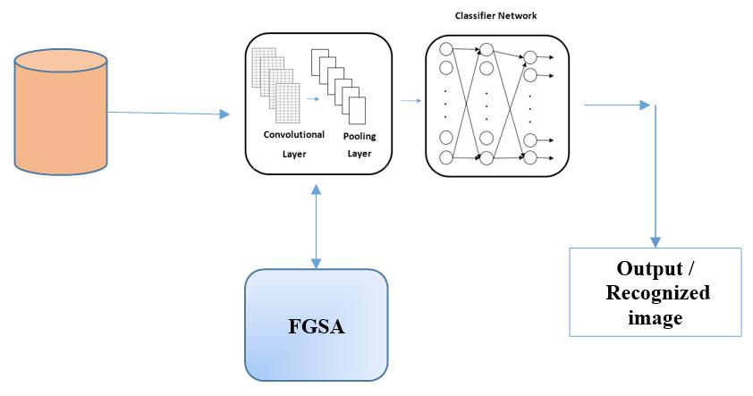
3. General proposal

4. Details when the CNN works together with FGSA

The FGSA generates a matrix of possible solutions in a designated range, for the Bsize it was searched between 10 to 100 random values to be generated, for the filter size between 1 to 10 and for the number of filters between 10 to 50. These values were considered because tests were performed, where each of the values to be optimized were modified manually and, therefore an estimated range of the best values to be used was obtained, in order to have a satisfactory result in the recognition of the images. In Table 1 we can notice a red rectangle, which designates the “Initial Matrix” that the FGSA generates in a random way, each row of the initial matrix is an agent (shown in the green rectangle) that has 3 dimensions: the first one is the value of the Bsize, the second value corresponds to the number of filters and finally the third value designates the value of the filter size of the convolution layer.

Tab. 1. Initial Matrix

3.1. Architecture of the CNN

In Table 2 shows the architecture of CNN, which will be used for each case study.

Input M * N -

Convolution

FGSA Obtain number and Size of filter of convolution (x*x) ReLU

Pooling 1 layer, medium (2*2) -

Hidden layers 100 nodes ReLU

Output 40/38 nodes Softmax

3.2. Variables to Be Optimized

For the CNN optimization, three main variables were selected, which will help the network obtain a better recognition percentage.

Based on previous experiments [40], it was shown that varying the value of Bsize has a great influence on the training of the network, since the Bsize selects the training data and calculates the adjustment or updating of the weights, this contributes to the network training faster because it repeats the process fewer times and this decreases the training time.

The variables that were considered to be optimized are the following:

1. The number of blocks: is the variable that blocks all the images that will enter the training stage in the convolutional neural network.

2. The number of filters: this parameter is used in the convolution layer, it is the number of filters to be used in this layer, which obtain the characteristics map.

3. Filter size: is the variable that is used to define the filter size of the convolution layer, which extracts the data to form the characteristics map.

Figure 5 shows the detailed development of how the FGSA method contemplates the optimization of the considered variables for a better result of the image pattern recognition of the CNN, using the variables of Bsize which, as mentioned above, are responsible for dividing the input images to pass to network

Fig.

Fig.

Fig. 5. Detail of process when FGSA optimized variables

training, the number of filters that determines the number of feature maps to be extracted from the image and the size of the filter in the convolution layer, which takes the sample size to form the feature map.

4. Results and Discussion

In this experiment, tests were performed with a CNN using the FGSA to optimize it, using for this case study the ORL database, which contains 400 images of human faces, this consists of 40 humans and 10 images taken at different angles of the face of each of them, with a size of 112 * 92 pixels in .pgm format for each image. In Figure 6 we can find some examples of the ORL database, the parameters used for the CNN are shown in Table 3, as well as the parameters used in the FGSA method are presented in Table 4, once this experiment was completed, it was concluded with the results presented in Table 5, where the highest recognition value is 91.25% when the value of Bsize is 37.

Table 6 presents the results obtained from the manual modification of the “Bsize” value in the CNN using 20 filters of 9*9, it is verified that the optimal value (obtained by the FGSA) is when the value of Bsize is 37. The test was performed where the Bsize value is modified from 10 in 10 to reach the value of 100. With this test, the highest recognition rate was 91.25 %.

Once the FGSA has found the best Bsize parameter with a value of 37, it starts with the optimization of the next value. For this test, a simulation was performed, where the value of the number of filters used in the convolution layer is modified manually. As a result of this test, the best value for the number of filters in the network is 20, because it consumes less resources and processing time, although when the number of filters is 50, it also reaches the same percentage of recognition that is 91.25 %, but with the difference that it consumes more resources and time. The results can be found in Table 7.

Fig. 6. Images from the ORL database

Tab. 3. Parameters of CNN for the ORL database

Tab. 4. Parameters of the FGSA

Tab. 5. Results of Bsize optimized with

Tab. 6. Bsize modified manually from CNN using ORL without FGSA

Tab. 7. Number of filter is manually modified

In Table 8 the results of 15 experiments can be observed, where the Bsize value is 37; the value of the number of filters of the convolution layer belonging to the CNN was optimized, obtaining that the best result is when the number of filters in this layer is 20, which results in a recognition of 91.25% of the ORL image database.

8. Number of filters optimized with FGSA

In Table 9 it can be noted that the FGSA method optimized the filter size parameter of the convolution layer, using the optimal fixed parameters of Bsize in 37 and the number of filters in 20. The best value obtained for the optimized parameter is 3*3, resulting in a recognition percentage of 93.75 %.

Tab. 9. Size of filter optimized with FGSA

Tab. 10. Size of filter manually modified

Tab.

Tab. 11. Comparative with others methods using the ORL database

In order to confirm the results presented in Table 9, a manual experiment was carried out. In this test, the Bsize and the number of filters are fixed, with a value of 37 and 20 respectively; but, on the other hand, the filter size parameter was modified manually. It was observed that when the size of the filter is an even number, at the time of pooling the data does not coincide with the operations performed, whereas when the filter size is an odd number, the pooling operations conclude without problems. Table 10 shows the results achieved in this manual experiment; where the best obtained result is when the filter size has a value of 3 * 3 with a recognition rate of 93.75%.

Table 11 presents a comparison of other methods and their maximum recognition percentages obtained using different neural networks, such as monolithic and modular neural networks. The results of the CNN are compared with the results published in other works where other types of neural networks are implemented, some of the results of these networks are better than those of CNN because they use methods of preprocessing, response integrators, modularity as well as cross-validation methods for data selection. Table 12 shows the data used in the performed experiments.

In order to verify that the result of the FGSA method is the best, the manual test was performed where the Bsize parameter is modified with values of 10 in

10 in which it can be verified that the best result is when the Bsize value is 38, we can visualize these results in Table 16, since; although with other parameters (20 and 30) we also obtain the same percentage of recognition in the solution that the FGSA produces, it takes less time; therefore, it uses less processing time.

Tab. 12. Data used for the comparison with others methods

In other case of study the CROPPED YALE database was used, which contains 380 images of human faces of 192 * 168 pixels in .pgm format, they are 38 people with 10 images for each of them, some examples of this data base are present in Figure 7. Table 13 details the parameters used for the CNN, as well as in Table 14, describes the parameters used of the FGSA method.

In Table 15 we can find the results obtained by running the CNN using the FGSA to optimize the Bsize variable, where the best value for Bsize is 38 with a 100 % recognition rate.

Tab. 13. CNN parameters used for the CROPPED YALE database

parameters

Tab. 14. FGSA parameters used with the case it CROPPED YALE

As can be seen in Table 17 the best value (38) of the Bsize parameter was maintained, this value was obtained based on the performed experiments. Manual tests were performed in which, the number of filters was modified, having as best recognition rate (100%) that the number of filters of the convolution layer is 20; although the same result was reached with the values of 50,60,70,80,90 and 100 in the number of filters, these require more computational resources and time to reach the same result. For this reason, it is concluded that the best value is 20, since it reaches the best recognition percentage in less time.

In Table 18, the results of 15 experiments are presented, the value of the Bsize is 38 and the number of filters of the convolution layer was optimized with the help of the FGSA method, thus achieving the best result in the number of filters, obtaining 100% image recognition from the CROPPED YALE database.

15. Bsize optimized using FGSA

Tab. 17. Results when the number of filters is modified manually

Fig. 7. Example of CROPPED YALE database

Tab.

Tab. 16. Results when the “Bsize” is manually modified

Tab. 18. Results when the number of filters is optimized with FGSA

Tab. 19. Data used for comparative methods using the CROPPED YALE database

4.1. The Best Architectures

Table 21 shows the collection of the best architectures found from the optimized values (Bsize, Number of filters and Filter Size), performing 15 experiments per each database. For the ORL database we obtained the 93.75% recognition rate when the number of blocks or Bsize are 37 and the filter size are 3*3, while for the CROPPED YALE database obtained 100% recognition rate when the parameter Bsize is 38, in Both cases the number of filters is 20.

5. Conclusion

Next, the data used for several experiments can be found in Table 19, thus having the comparison of other methods using different types of neural network such as Modular and Monolithic and their percentages of recognition in Table 20, where they used response integrators, as well as the pre-processing of images, modularity and cross-validation methods for data selection.

Based on the experiments performed with the Convolutional Neuronal Network, it is concluded that these neural networks help the recognition of images, since, they are designed for these uses; however, if an optimization method is applied to these CNN, such as in this case it was the FGSA method, they have better results and help to obtain the architecture to arrive at a more optimal solution in pattern recognition applications.

Tab. 20. Comparative CNN with others methods using CROPPED YALE database

Tab. 21. The best architecture for each case

37 20 3*3

YALE 38 20 9*9

It was demonstrated that the optimization methods are reliable and the obtained results with these are the same as the tests performed manually, where the values of “Bsize”, number of filters and filter size were varied in the CNN, which, verifies that the optimization method (FGSA) represents a good way to find and build the best architecture of the network. Resulting in a high recognition percentage in the case studies presented.

It is also planned to optimize other parameters of the CNN, as well as to search for another architecture of the network, modifying the number of layers and neurons per layer in the classification or adding convolution, to obtain better models and these can be applied to any pattern recognition problem.

It is considered that with more time we can perform deeper explorations, such as increasing the number of agents in the FGSA and the number of iterations/experiments, in this way, we will probably obtain better percentages of recognition and reduce the processing time. As future work, type-2 fuzzy logic could be incorporated to improve results [43-44].

A CKNO w L e DG e M e NTS

We thank our sponsor CONACYT and Tijuana Institute of Technology for the financial support provided with the scholarship number 816488.

AUTHORS

Yutzil Poma – Tijuana Institute of Technology, B.C., Tijuana, México, e-mail: yutpoma@hotmail.com.

Patricia Melin* – Tijuana Institute of Technology, B.C., Tijuana, México, e-mail: pmelin@tectijuana.mx.

Claudia I. González – Tijuana Institute of Technology, B.C., Tijuana, México, e-mail: cgonzalez@tectijuana.mx.

Gabriela E. Martinez – Tijuana Institute of Technology, B.C., Tijuana, México, e-mail: gmartinez@tectijuana.mx.

*Corresponding author

Re F e R e NC e S

[1] D. H. Hubel and T. N. Wiesel, “Receptive fields, binocular interaction and functional architecture in the cat’s visual cortex”, The Journal of Physiology, vol. 160, no. 1, 1962, 106–154.

[2] K. Fukushima, “Neocognitron: A self-organizing neural network model for a mechanism of pattern recognition unaffected by shift in position”, Biological Cybernetics, vol. 36, no. 4, 1980, 193–202, DOI: 10.1007/BF00344251.

[3] Y. LeCun, B. E. Boser, J. S. Denker, D. Henderson, R. E. Howard, W. E. Hubbard and L. D. Jackel, “Handwritten Digit Recognition with a BackPropagation Network”. In: D. S. Touretzky (eds.), Advances in Neural Information Processing Systems 2, 1990, 396–404.

[4] D. Sánchez, P. Melin and O. Castillo, “Fuzzy Adaptation for Particle Swarm Optimization for Modular Neural Networks Applied to Iris Recognition”. In: P. Melin, O. Castillo, J. Kacprzyk, M. Reformat and W. Melek (eds.), Fuzzy Logic in Intelligent System Design, 2018, 104–114, DOI: 10.1007/978-3-319-67137-6_11.

[5] F. Valdez, O. Castillo and P. Melin, “Ant colony optimization for the design of Modular Neural Networks in pattern recognition”. In: 2016 International Joint Conference on Neural Networks (IJCNN), 2016, 163–168, DOI: 10.1109/IJCNN.2016.7727194.

[6] C. I. Gonzalez, J. R. Castro, O. Mendoza and P. Melin, “General type-2 fuzzy edge detector applied on face recognition system using neural networks”. In: 2016 IEEE International Conference on Fuzzy Systems (FUZZ-IEEE), 2016, 2325–2330, DOI: 10.1109/FUZZ-IEEE.2016.7737983.

[7] G. E. Martínez, P. Melin, O. D. Mendoza and O. Castillo, “Face Recognition with a Sobel Edge Detector and the Choquet Integral as Integration Method in a Modular Neural Networks”. In: P. Melin, O. Castillo and J. Kacprzyk (eds.), Design of Intelligent Systems Based on Fuzzy Logic, Neural Networks and Nature-Inspired Optimization, 2015, 59–70.

[8] P. Melin, I. Miramontes and G. Prado-Arechiga, “A hybrid model based on modular neural networks and fuzzy systems for classification of blood pressure and hypertension risk diagnosis”, Expert Systems with Applications, vol. 107, 2018, 146–164, DOI: 10.1016/j.eswa.2018.04.023.

[9] F. Valdez, P. Melin and O. Castillo, “Modular Neural Networks architecture optimization with a new nature inspired method using a fuzzy combination of Particle Swarm Optimization and Genetic Algorithms”, Information Sciences, vol. 270, 2014, 143–153, DOI: 10.1016/j.ins.2014.02.091.

[10] P. Melin, D. Sánchez and O. Castillo, “Genetic optimization of modular neural networks with fuzzy response integration for human recognition”, Information Sciences, vol. 197, 2012, 1–19, DOI: 10.1016/j.ins.2012.02.027.

[11] P. Melin and D. Sánchez, “Multi-objective optimization for modular granular neural net-

works applied to pattern recognition”, Information Sciences, vol. 460-461, 2018, 594–610, DOI: 10.1016/j.ins.2017.09.031.

[12] D. Sánchez, P. Melin and O. Castillo, “Optimization of modular granular neural networks using a firefly algorithm for human recognition”, Engineering Applications of Artificial Intelligence, vol. 64, 2017, 172–186, DOI: 10.1016/j.engappai.2017.06.007.

[13] F. Gaxiola, P. Melin, F. Valdez, J. R. Castro and O. Castillo, “Optimization of type-2 fuzzy weights in backpropagation learning for neural networks using GAs and PSO”, Applied Soft Computing, vol. 38, 2016, 860–871, DOI: 10.1016/j.asoc.2015.10.027.

[14] P. Melin, J. Amezcua, F. Valdez and O. Castillo, “A new neural network model based on the LVQ algorithm for multi-class classification of arrhythmias”, Information Sciences, vol. 279, 2014, 483–497, DOI: 10.1016/j.ins.2014.04.003.

[15] Y. LeCun, L. Bottou, Y. Bengio and P. Haffner, “Gradient-Based Learning Applied to Document Recognition”, Proceedings of the IEEE, vol. 86, no. 11, pp. 2278–2324, DOI: 10.1109/5.726791.

[16] A. Frome, G. Cheung, A. Abdulkader, M. Zennaro, B. Wu, A. Bissacco, H. Adam, H. Neven and L. Vincent, “Large-scale privacy protection in Google Street View”. In: 2009 IEEE 12th International Conference on Computer Vision, 2009, 2373–2380, DOI: 10.1109/ICCV.2009.5459413.

[17] R. Hadsell, P. Sermanet, J. Ben, A. Erkan, M. Scoffier, K. Kavukcuoglu, U. Muller and Y. LeCun, “Learning long-range vision for autonomous off-road driving”, Journal of Field Robotics, vol. 26, no. 2, 2009, 120–144, DOI: 10.1002/rob.20276.

[18] A. Sombra, F. Valdez, P. Melin and O. Castillo, “A new gravitational search algorithm using fuzzy logic to parameter adaptation”. In: 2013 IEEE Congress on Evolutionary Computation, 2013, 1068–1074, DOI: 10.1109/CEC.2013.6557685.

[19] E. Rashedi, H. Nezamabadi-pour and S. Saryazdi, “GSA: A Gravitational Search Algorithm”, Information Sciences, vol. 179, no. 13, 2009, 2232–2248, DOI: 10.1016/j.ins.2009.03.004.

[20] O. P. Verma and R. Sharma, “Newtonian Gravitational Edge Detection Using Gravitational Search Algorithm”. In: 2012 International Conference on Communication Systems and Network Technologies, 2012, 184–188, DOI: 10.1109/CSNT.2012.48.

[21] A. Hatamlou, S. Abdullah and Z. Othman, “Gravitational search algorithm with heuristic search for clustering problems”. In: 2011 3rd Conference on Data Mining and Optimization (DMO), 2011, 190–193, DOI: 10.1109/DMO.2011.5976526.

[22] S. Mirjalili, S. Z. Mohd Hashim and H. Moradian Sardroudi, “Training feedforward neural networks using hybrid particle swarm optimization and gravitational search algorithm”, Applied Mathematics and Computation, vol. 218, no. 22, 2012, 11125–11137, DOI: 10.1016/j.amc.2012.04.069.

[23] S. Mirjalili and S. Z. M. Hashim, “A new hybrid PSOGSA algorithm for function optimization”. In: 2010 International Conference on Computer and Information Application , 2010, 374–377, DOI: 10.1109/ICCIA.2010.6141614.

[24] I. Goodfellow, Y. Bengio and A. Courville, Deep learning, MIT Press, 2016.

[25] C. C. Aggarwal, Neural Networks and Deep Learning: A Textbook, Springer International Publishing, 2018.

[26] “Greedy Layer-Wise Training of Deep Networks”. Y. Bengio, P. Lamblin, D. Popovici and H. Larochelle, http://papers.nips.cc/ paper/3048-greedy-layer-wise-training-ofdeep-networks.pdf. Accessed on: 2020-06-23.

[27] E. de la Rosa Montero, “El aprendizaje profundo para la identificación de sistemas no lineales,” Thesis, Centro de Investigación y de Estudios Avanzados del Instituto Politécnico Nacional, Mexico, 2014 (In Spanish), https:// www.ctrl.cinvestav.mx/~yuw/pdf/MaTesER. pdf. Accessed on: 2020-06-23.

[28] Y. LeCun and Y. Bengio, “Convolutional networks for images, speech, and time series”. In: The handbook of brain theory and neural networks, 1998, 255–258.

[29] Y. Bengio and P. Lamblin, “Greedy layer-wise training of deep networks,” Adv. neural, no. 1, pp. 153–160, 2007.

[30] K. Chellapilla, S. Puri and P. Simard, “High Performance Convolutional Neural Networks for Document Processing,” In: Tenth International Workshop on Frontiers in Handwriting Recognition, La Baule (France), Suvisoft, 2006.

[31] V. Nair and G. E. Hinton, “Rectified linear units improve restricted boltzmann machines”. In: Proceedings of the 27th International Conference on Machine Learning, 2010, 807–814.

[32] M. Ranzato, F. J. Huang, Y.-L. Boureau and Y. LeCun, “Unsupervised Learning of Invariant Feature Hierarchies with Applications to Object Recognition”. In: 2007 IEEE Conference on Computer Vision and Pattern Recognition, 2007, 1-8, DOI: 10.1109/CVPR.2007.383157.

[33] J. Yang, K. Yu, Y. Gong and T. Huang, “Linear spatial pyramid matching using sparse coding for image classification”. In: 2009 IEEE Conference on Computer Vision and Pattern Recognition, 2009, 1794–1801, DOI: 10.1109/CVPR.2009.5206757.

[34] T. Wang, D. J. Wu, A. Coates and A. Y. Ng, “Endto-end text recognition with convolutional

neural networks”. In: Proceedings of the 21st International Conference on Pattern Recognition, 2012, 3304–3308.

[35] P. Kim, MATLAB Deep Learning: With Machine Learning, Neural Networks and Artificial Intelligence, Berkeley, California: Apress, 2017, DOI: 10.1007/978-1-4842-2845-6.

[36] R. Venkatesan and B. Li, Convolutional Neural Networks in Visual Computing: A Concise Guide, CRC Press, 2017.

[37] L. Lu, Y. Zheng, G. Carneiro, and L. Yang, (eds.), Deep Learning and Convolutional Neural Networks for Medical Image Computing: Precision Medicine, High Performance and Large-Scale Datasets, Springer International Publishing, 2017.

[38] B. González, F. Valdez, P. Melin and G. PradoArechiga, “Fuzzy logic in the gravitational search algorithm for the optimization of modular neural networks in pattern recognition”, Expert Systems with Applications, vol. 42, no. 14, 2015, 5839–5847, DOI: 10.1016/j.eswa.2015.03.034.

[39] B. González, F. Valdez, P. Melin and G. PradoArechiga, “Fuzzy logic in the gravitational search algorithm enhanced using fuzzy logic with dynamic alpha parameter value adaptation for the optimization of modular neural networks in echocardiogram recognition”, Applied Soft Computing , vol. 37, 2015, 245–254, DOI: 10.1016/j.asoc.2015.08.034.

[40] Y. Poma, P. Melin, C. I. González and G. E. Martínez, “Optimal Recognition Model Based on Convolutional Neural Networks and Fuzzy Gravitational Search Algorithm Method”. In: O. Castillo and P. Melin (eds.), Hybrid Intelligent Systems in Control, Pattern Recognition and Medicine, 2020, 71–81, DOI: 10.1007/978-3-030-34135-0_6.

[41] C. I. González, P. Melin, J. R. Castro, O. Mendoza and O. Castillo, “General Type-2 Fuzzy Edge Detection in the Preprocessing of a Face Recognition System”. In: P. Melin, O. Castillo and J. Kacprzyk (eds.), Nature-Inspired Design of Hybrid Intelligent Systems, 2017, 3–18, DOI: 10.1007/978-3-319-47054-2_1.

[42] G. E. Martínez, O. Mendoza, J. R. Castro, A. Rodríguez-Díaz, P. Melin and O. Castillo, “Comparison between Choquet and Sugeno integrals as aggregation operators for pattern recognition”. In: 2016 Annual Conference of the North American Fuzzy Information Processing Society (NAFIPS), 2016, 1–6, DOI: 10.1109/NAFIPS.2016.7851628.

[43] P. Melin, J. Urias, D. Solano, M. Soto, M. Lopez and O. Castillo, “Voice Recognition with Neural Networks, Type-2 Fuzzy Logic and Genetic Algorithms”, Engineering Letters, vol. 13, no. 2, 2006.

[44] F. Gaxiola, P. Melin, F. Valdez, J. R. Castro and O. Castillo, “Optimization of type-2 fuzzy weights in backpropagation learning for neural networks using GAs and PSO”, Applied Soft Computing, vol. 38, 2016, 860–871, DOI: 10.1016/j.asoc.2015.10.027.