Broad Street Scientific 2023-2024

BROAD STREET SCIENTIFIC

The North Carolina School of Science and Mathematics – Durham Journal of Student STEM Research

Front Cover

Caught by NASA’s SDO satellite, the Sun’s “smile” is actually made up of coronal holes. These dark spots, while invisible to the naked eye, can be seen through UV light and appear when areas of the Sun are less heated and dense than their surrounding plasma.

Credit: NASA’s Solar Dynamics Observatory

Biology Section

This image depicts a Cleopatra (Gonepteryx cleopatra) butterfly resting on a Rudbeckia hirta flower. The left side shows the butterfly and flower under a UV light while the right side shows them in the visible light spectrum

Credit: (C) Dr. Klaus Schmitt, Weinheim Germany uvir.eu used with permission of the artist

Chemistry Section

The “Fantasy Rock” is composed of multiple minerals from the Taseq Slope in Greenland. Typically, the rock consists of tugtupite, sodalite, chkalovite, and analcime. Under UV light, the composition of these minerals produces bright, fluorescent colors

Credit: (C) www.minershop.com used with permission

Engineering Section

These miniature UV LED lights are popular in recreational projects for their versatility. Practical uses of UV light include disinfection, sterilization, and forensics.

Credit: (C) adafruit.com used with permission

Mathematics and Computer Science Section

This image shows a white rose photographed under UV light; it appears pink and has glowing white spots. The petals of the rose follow the Fibonacci sequence, where a new set grows between the spaces of the previous set.

Credit: Craig P. Burrows https://cpburrows.com/

Physics Section

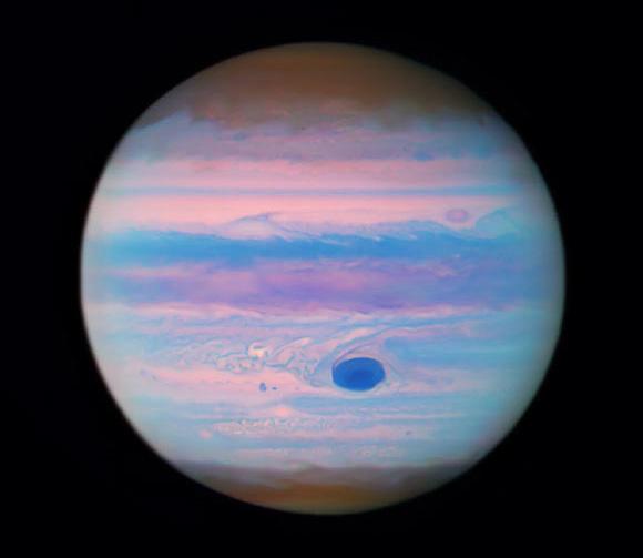
The Hubble Space Telescope took this picture of Jupiter in the UV spectrum. The famous Great Red Spot, which appears blue in UV light due to high altitude particles absorbing light at these wavelengths, is large enough to swallow the Earth.

Credit: NASA / ESA / Hubble / M. Wong, University of California, Berkeley / Gladys Kober, NASA & Catholic University of America

7 Essay: Is It Possible to Use GPS to Combat Climate Change?

TERESA FANG, 2025 9 Photography: Grog

CHARLOTTE GOEBEL, 2025

La Fortuna Waterfall

VINCENT SHEN, 2025

10 Reduction of the Abundance of Antibiotic-Resistant Bacteria (ARB) in Contaminated Soil using Modified Biochar

EMILY ALAM, 2024

20 Identification of Single-Nucleotide Polymorphisms Related to the Phenotypic Expression of Drought Tolerance in Oryza Sativa

REVA KUMAR, 2024

26 Analyzing the Effect of Inhibiting Combinations of Protein Kinases on the Progression of Alzheimer’s Disease in Caenorhabditis Elegans

GAURI MISHRA, 2024

35 Design and Synthesis of a PROTAC Molecule and a CLIPTAC Molecule for the Treatment of Alzheimer's Disease by p-Tau Degradation through the Ubiquitin Proteasome System

OLIVIA AVERY, 2024

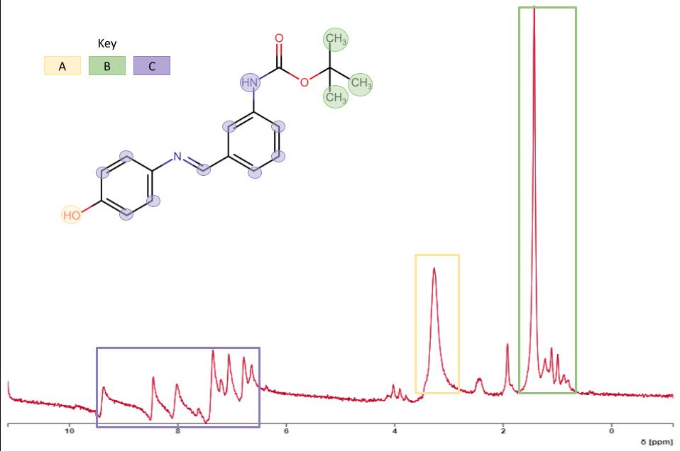
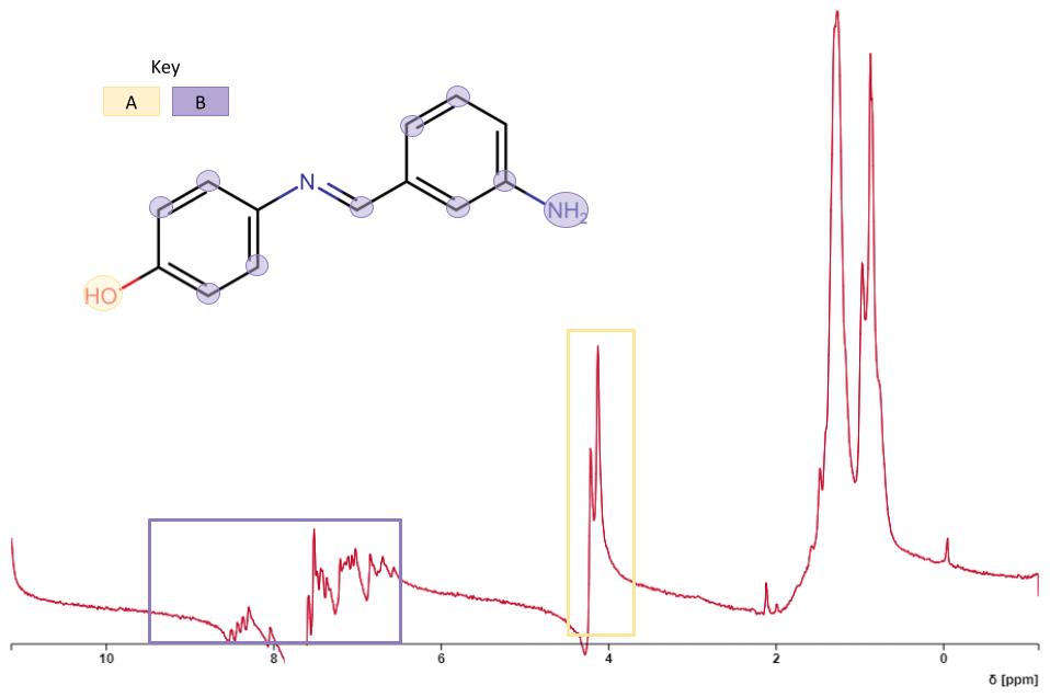
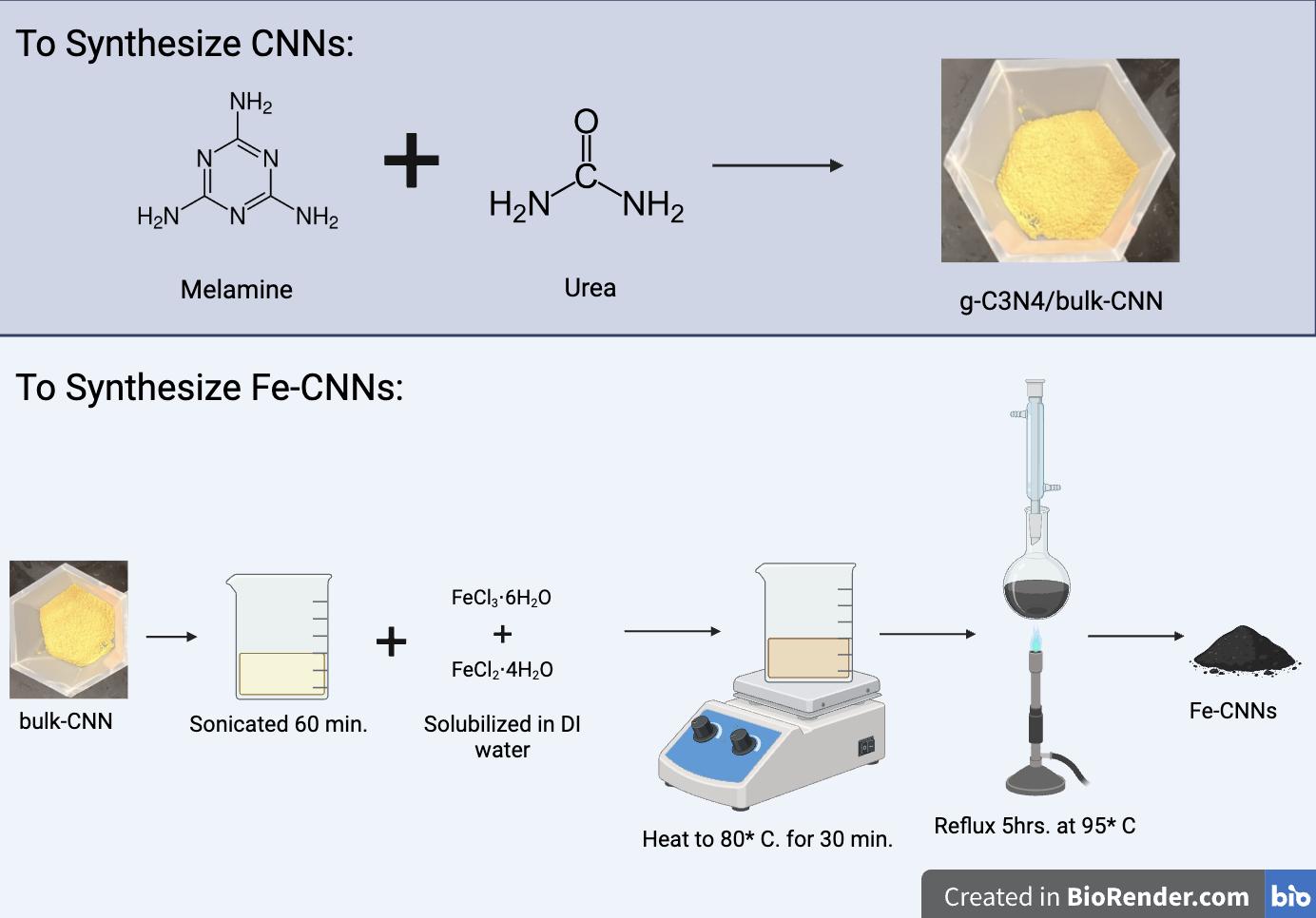
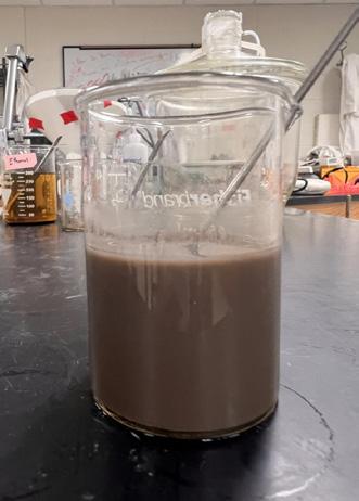
45 Analyzing NOx Removal Efficiency and Washing Resistance of Iron Oxide Decorated g-C3N4 Nanosheets Attached to Recycled Asphalt Pavement Aggregate

EMMIE ROSE, 2024

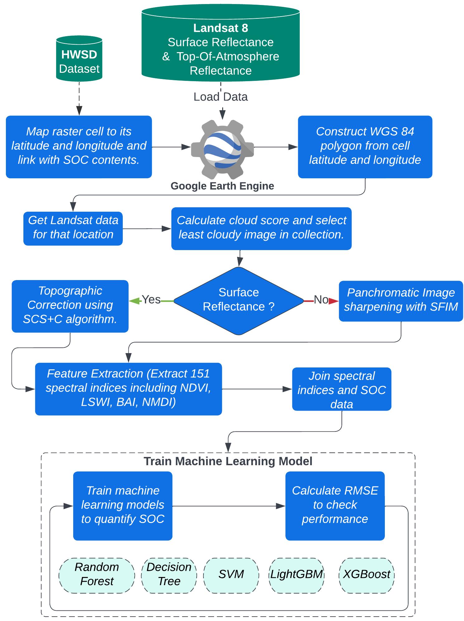
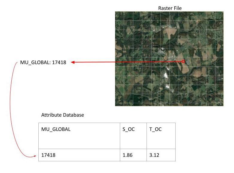
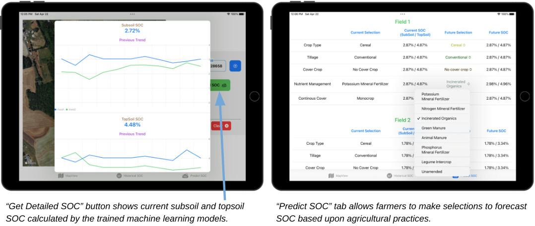
51 Mapping Soil Organic Carbon Using Multispectral Satellite Imagery and Machine Learning

REYANSH BAHL, 2024 ONLINE

58 ASDAware: A Low-Cost Eye Tracking-Based Machine Learning Model for Accurate

Autism Spectrum Disorder Risk Assessment in Children

ISHAN GHOSH AND SYED SHAH, 2024 ONLINE

Mathematics and Computer Science

65 A Problem in Game Theory and Calculus of Variations

CHRISTOPHER BOYER 2024, GRACE LUO 2025, AND SIDDHARTH PENMETSA 2024

74 On Mosaic Invariants of Knots

VINCENT LIN, 2024

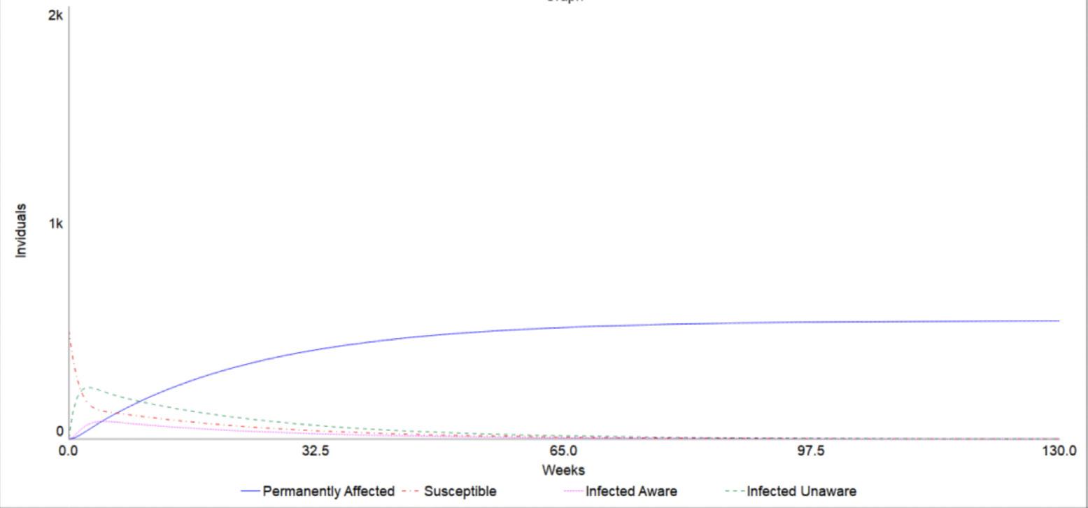
82 Computational Model of Gonorrhea Transmission in Rural Populations

DIYA MENON, 2025 ONLINE Physics

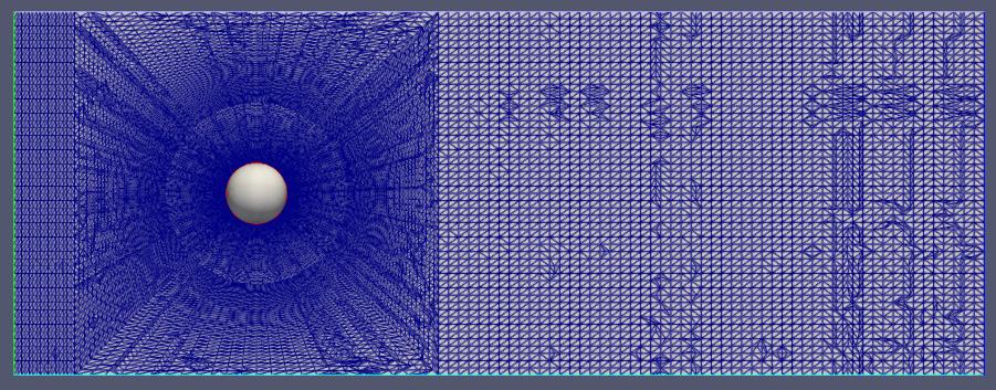
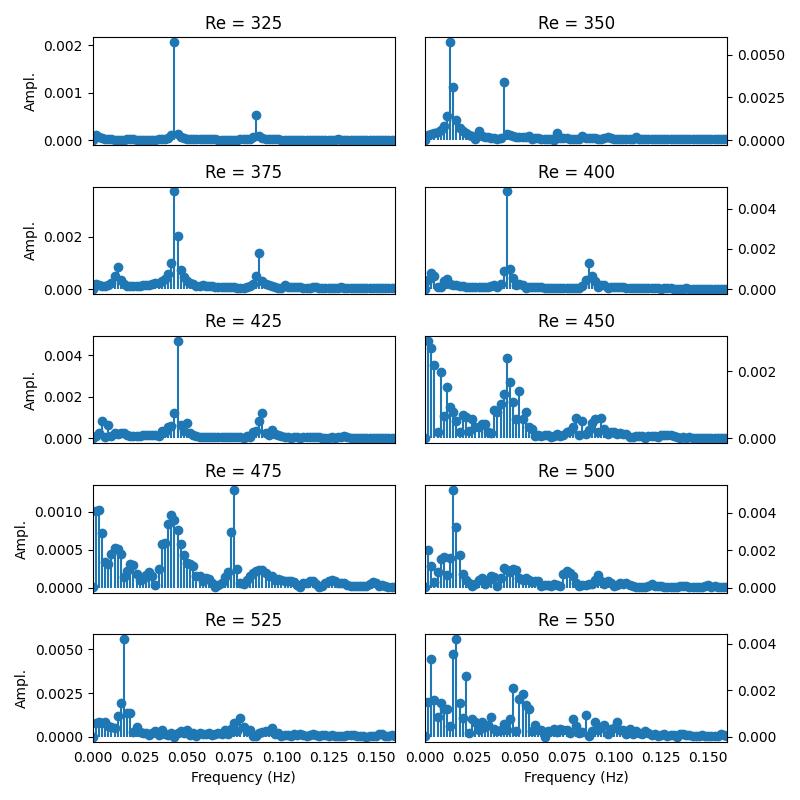
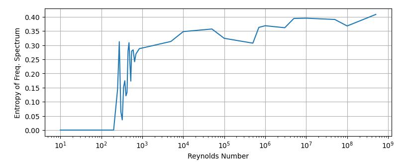
90 Using Spectral Entropy as a Measure of Chaos to Quantify the Transition from Laminar to Turbulent Flow

MATTHEW LEE, 2024

97 Detection of the Warm-Hot Intergalactic Medium Between the Coma and Leo Clusters

LIKHITA TINGA, 2024

Featured Article

103 An Interview with Dr. Richard McLaughlin

LETTER from the CHANCELLOR

“It is a capital mistake to theorize before one has data. Insensibly one begins to twist facts to suit theories, instead of theories to suit facts.”

I am proud to introduce the thirteenth edition of the North Carolina School of Science and Mathematics’ (NCSSM) scientific journal, Broad Street Scientific. Each year students at NCSSM conduct significant scientific research, and Broad Street Scientific is a student-led and student-produced showcase of some of the impressive research being done by students on our Durham campus.

For more than four decades now we have provided research opportunities for NCSSM students from all across North Carolina. I am proud of how these opportunities have helped inspire many of our alumni to research and innovate, creating new companies and novel approaches to tackle some of our world’s most challenging problems. The research reflected in this journal highlights just a sample of the incredible work NCSSM students are doing today, building their foundation as the next generation of scientists and innovators who will undoubtedly change our state and the world for the better in the years to come.

Opened in 1980, NCSSM was the nation’s first public residential high school where students study a specialized curriculum emphasizing science and mathematics. Teaching students to do research and providing them with opportunities to conduct high-level research in biology, chemistry, physics, computational science, engineering and computer science, mathematics, humanities, and the social sciences is a critical component of NCSSM’s mission to educate academically talented students to become state, national, and global leaders in science, technology, engineering, and mathematics. More than eighty-percent of NCSSM students conduct research in their two years at NCSSM. I am grateful for

~Sir Arthur Conan Doyle

our talented NCSSM faculty and mentors at institutions across our state who provide these incredible opportunities for students, on two campuses and in our online program, to learn research methods and conduct high quality research.

Each edition of Broad Street Scientific features some of the best research students conduct at NCSSM under the guidance of our outstanding faculty and in collaboration with researchers at major universities and other research institutions. For thirty-nine years, NCSSM has showcased student research through our annual Research Symposium each spring and at major research competitions such as the Regeneron Science Talent Search and the International Science and Engineering Fair. Amazing things happen when you bring talented student researchers together with incredible faculty, which was highlighted this year as ten NCSSM students were named Regeneron Scholars. The publication of this journal provides another opportunity to share with the broader community the outstanding research being conducted by NCSSM students.

I would like to thank all of the students and faculty involved in producing Broad Street Scientific, particularly faculty sponsors Dr. Jonathan Bennett and Dr. Michael Falvo and senior editors Phoebe Chen, Keyan Miao, and Jane Shin. Explore and enjoy!

Dr. Todd Roberts Chancellor

WORDS from the EDITORS

Welcome to the Broad Street Scientific, NCSSM Durham’s official journal of student research in science, technology, engineering, and mathematics. This past year has been one of significant change as we reworked the publication process and outlined our AI policy as we saw the rise of AI technology. These improvements in our 13th edition allow us to continue showcasing exceptional research, innovative ideas, and collaboration within the students of North Carolina School of Science and Mathematics. As you turn these pages, you will find investigations ranging from disease transmission models to galaxy clusters, with each sharing the same goal of advancing our understanding of the world.

Addressing these developments has required a new perspective, which is reflected in our theme for this year, ultraviolet. Nature contains hidden stories, from the smiling sun to fluorescing flowers, yet it takes research and the development of new technologies to perceive what our eyes cannot. And yet simply seeing is not enough: in an age where we are more divided than ever and AI image generation is blurring the lines between real and not, the truth is more elusive than ever. Ultraviolet reminds us that we must keep an open mind and embrace diversity, celebrating the opportunities brought by combining different perspectives.

We would like to thank the faculty, staff, and administration of NCSSM, particularly Chancellor Dr. Todd Roberts, Dean of Science Dr. Amy Sheck, and Director of Mentorship and Research Dr. Sarah Shoemaker. They continue to support and nurture a stimulating academic environment that encourages motivated students to apply their interests towards solving real-world problems. For the next generation of young people who will no doubt change the world, NCSSM serves as a nurturing environment of passion and determination. We extend special thanks to Dr. Jonathan Bennett and Dr. Michael Falvo for their invaluable support and guidance throughout the publication process. Lastly, we would like to acknowledge Dr. Richard McLaughlin, Professor of Mathematics at UNC Chapel Hill, for speaking with us about his experience in fluid dynamics research and imparting important advice to young scientists so that we may each define our unique perspectives and shape the world around us.

Jane

Shin, Keyan Miao, and Phoebe Chen

Editors-in-Chief

BROAD STREET SCIENTIFIC STAFF

Editors-in-Chief

Phoebe Chen, 2024 Durham

Keyan Miao, 2024 Durham

Jane Shin, 2024 Durham

Publication Editors

Snigdha Agasthyaraju, 2024 Online

Advika Arun, 2025 Durham

Jessily Chen, 2024 Durham

Florence Cheung, 2025 Durham

Kelly Fung, 2025 Durham

Paisley Holland, 2025 Durham

Biology Editors

Aadi Kucheria, 2025 Durham

Jiah Lee, 2025 Durham

Skyler Qu, 2025 Durham

Marcella Willett, 2024 Online

Chemistry Editors

Cathy Deng, 2025 Durham

Nishanth Gaddam, 2025 Online

Nikhil Vemuri, 2025 Durham

Engineering Editors

Caroline Downs, 2025 Durham

Adrian Tejada, 2025 Durham

Mathematics and Computer Science Editors

Physics Editors

Vishnu Vanapalli, 2025 Durham

Markandeya Yalamanchi, 2025 Durham

Teresa Fang, 2025 Durham

Ian Suh, 2025 Durham

Faculty Advisors

Dr. Jonathan Bennett

Dr. Michael Falvo

IS IT POSSIBLE TO USE GPS TO COMBAT CLIMATE CHANGE?

Teresa Fang

Teresa Fang was selected as the winner of the 2024 Broad Street Scientific Essay Contest. Her award included the opportunity to interview Dr. Richard McLaughlin, Professor of Mathematics at the University of North Carolina at Chapel Hill.

Despite the Global Positioning System (GPS) being well known, few are aware of an alternative use of its signals. Aside from providing directions to the nearest café or restaurant, GPS can revolutionize remote sensing, serving as a tool to predict natural disasters and combat climate change.

GPS is a tool for remote sensing. At its core, remote sensing is communication through electromagnetism. It relies on two things: a transmitter and a receiver. A satellite’s transmitter will encode a message through various bands of electromagnetic frequencies using modulation, changing data into waves [1]. A receiver will then pick those up and transform the waves back into analytical data. Depending on factors like distance apart, size of antennas, types of electromagnetic transmission, bandwidth, or limiting power, different kinds of data can be measured and transmitted.

At present, GPS consists of a network of 31 broadcasting satellites orbiting Earth at an altitude of around 20,000 km. While normal radar satellites have both their receiver and transmitters on the satellites, GPS has receivers on the ground, listening and interpreting microwave satellite transmission [1]. This means that at any point on the Earth’s surface, you are in the range of at least four satellites tracking the intersection of three physical dimensions, along with time, through trilateration. In an everyday example, your phone is the receiver to those four satellites’ transmitters to pinpoint your real-time location on Earth.

But what makes GPS an ideal tool to revolutionize remote sensing? After all, GPS is just a type of microwave radar system with a different scattering geometry than other systems, and microwave radar has been used for years to detect changes in Earth’s surface.

GPS reflectometry is one of the three techniques that have untapped potential for studying and combating climate change [2]. The two others are occultation, which measures the vertical gradient of the atmospheric index, and scatterometry, which scatters signals over targets like water to measure wind properties [3][4]. GPS signals are circularly polarized L-band signals (1-2 GHz range, at 19 or 24 cm specifically for GPS), which means they are

unaffected by cloud cover and sunlight, thus making it easier to measure strong versus weak signals from surfaces with large changes in dielectric constants, such as wet soil or sea ice [5]. This system allows researchers to measure changes in the frequency, amplitude, or phase of the interference pattern of a reflected surface to draw observations and collect pinpointed data quickly.

But rather than just having satellites track climate change, satellites may contribute to “solving” climate change through the bidirectional reflectance distribution function (BRDF). The BRDF fr (wi , wr ) determines a surface’s reflected energy in terms of incoming and reflected radiance [6]. Using the measured BRDFs of a known surface, BRDF can be applied to a much larger scope to image a larger surface, such as Earth. By adding more variables to the BRDF, we can potentially evaluate the parameters of a climate change model, i.e. with a multivariable function

fr(wi , wr , T, Vw , Vc , Ms ) where T represents temperature, V w represents wind speed, V c represents water current speed, M s represents soil moisture, etc.

GPS signals can provide the necessary information, in the form of microwaves, to model such a function. As a pioneering technique, GPS reflectometry is a promising approach to measuring and modeling hydrologic effects, such as icebergs or Arctic sea ice [6]. As a tool to combat climate change, these satellites give us an overhead and underwater view to make models, find melt rates, and potentially find ways to offset rising sea levels in the long run. While normal radar satellites have difficulty measuring ice thickness, GPS signals have long wavelengths to penetrate that canopy. If we can also measure the levels of greenhouse gases in the atmosphere, we could evaluate the correlation of greenhouse gases with the rate of sea ice melting and develop predictability models using the multivariable BRDF to mimic both short-term and long-term climate changes.

Although several other remote sensing techniques and instruments can retrieve the same information, the GPS reflection technique is cost-effective. GPS recycles

signals that already exist in the ionosphere, so there is no need for additional satellites or expensive microwave transmitters, such as the passive radiometers and active radars that NASA and CERN have been launching. For example, NASA’s eight-satellite CYGNSS constellation cost $152 million to study Earth’s hydrology, while CERN’s two-satellite Sentinel 1 constellation cost $385 million for the same purpose [8][9].

GPS reflectometry may be an avenue to revolutionize future satellite missions, as this technique is relatively cheap and can provide data complementary to existing data, filling gaps in our knowledge on select aspects. Launching constellations of GPS instruments would be interesting, as GPS constellations have a high temporal resolution or temporal repeat period. With multiple satellites collecting data over a location at the same time, frequently updated data are readily available, making the creation of both predictability models and near-realtime spatial resolution maps easier. This means people in affected communities can have more time to evacuate in times of disaster as forecasting is more accurate. As more and more research is being done into GPS reflectometry, finding alternatives to dealing with climate change may be less of a distant dream and more of an innovative reality.

[1] Schauer, Katherine. (2020, October 6). Space Communications: 7 Things You Need to Know. NASA. https://www.nasa.gov/missions/tech-demonstration/ space-communications-7-things-you-need-toknow/#:~:text=At%20its%20simplest%2C%20space%20 communications

[2] Baier, M. (n.d.). GPS occultation, reflectometry and scatterometry (gors) receiver technology based on COTS as quintessential instrument for future tsunami detection system. GPS Reflectometry. https://www.gitews.de/en/ gps-technology/gps-reflectometry/#:~:text=GPS%20 scatterometry%20and%20reflectometry%20 are,compensates%20for%20the%20low%20signal

[3] Eyre, J. R. (2008, June). An introduction to GPS radio occultation and its use in numerical weather prediction. In Proceedings of the ECMWF GRAS SAF workshop on applications of GPS radio occultation measurements (Vol. 1618).

[4] Center for Ocean-Atmospheric Prediction Studies (COAPS). (n.d.). Scatterometry - Overview. Scatterometry & Ocean Vector Winds. https://www.coaps.fsu.edu/ scatterometry/about/overview.php

[5] Chew, C. (2022). Water makes its mark on GPS signals. Physics Today, 75(2), 42–47. https://doi.org/10.1063/ Pt.3.4941

[6] Wynn, C. (2015, October 7). A basic introduction to BRDF-based lighting. Princeton University. https://www. cs.princeton.edu/courses/archive/fall06/cos526/tmp/ wynn.pdf

[7] Schild, K. M., Sutherland, D. A., Elosegui, P., & Duncan, D. (2021). Measurements of iceberg melt rates using high‐resolution GPS and iceberg surface scans. Geophysical Research Letters, 48(3). https://doi. org/10.1029/2020gl089765

[8] Harrington, J. D. (2023, July 26). NASA selects low cost, High Science Earth Venture Space System. NASA. https://www.nasa.gov/news-release/nasa-selects-lowcost-high-science-earth-venture-space-system/

[9] Clark, S. (2014, April 2). Europe’s Earth Observing System ready for liftoff. Soyuz launch report. https://spaceflightnow.com/soyuz/ vs07/140402preview/#:~:text=Levrini%20 said%20the%20Sentinel%201A,or%20%2492%20 million%2C%20he%20said

PHOTOGRAPHY: GROG & LA FORTUNA WATERFALL

Charlotte Goebel & Vincent Shen

Charlotte Goebel and Vincent Shen were selected as the winners of the 2024 Broad Street Scientific Photo Contest. Their awards included the opportunity to have their photographs featured in the 2024 volume of the Broad Street Scientific

Grog (Green Frog) by Charlotte Goebel

This American bullfrog (Lithobates catesbeianus) resides in a calm pond inlet of the Blue Ridge Mountains. Native to eastern North America, American bullfrogs are a globally invasive species, often destroying native amphibian populations. The rapidly multiplying bullfrogs exemplify the challenges of preserving natural habitats in a globalized world.

La Fortuna Waterfall by Vincent Shen

I captured this photograph of the 70-meter-high La Fortuna Waterfall in northwestern Costa Rica after a steep, sloping hike down. The dark, stratovolcanic rocks filter the plunging water above, which serves as the town of La Fortuna’s water supply.

REDUCTION OF

THE ABUNDANCE

OF ANTIBIOTIC-

RESISTANT BACTERIA (ARB) IN

CONTAMINATED

SOIL USING MODIFIED BIOCHAR

Emily Alam

Abstract

This research investigates the efficacy of modified biochar in mitigating the proliferation of antibiotic-resistant bacteria (ARB) in contaminated soil, focusing on samples from Oak Grove Farm, Wallace, NC. Soil bacteria were isolated and tested for resistance to multiple antibiotics. Experimental groups included pristine biochar and biochar modified with alkaline (KOH) or acidic (H₃PO₄) treatments. Results demonstrate a significant reduction in ARB abundance with modified biochar treatments compared to the control, with acidic modification proving the most effective. This study suggests that modified biochar has a promising outlook in reducing the transmission of antibiotics, antibiotic-resistant genes (ARGs), and ARB, offering a sustainable solution to combat antibiotic resistance in soil environments.

1. Introduction

Antibiotic treatment is the most common medicine prescribed to combat infection. However, as the list of infectious diseases and illnesses that rely on antibiotics as their primary treatment continues to grow, it becomes a less reliable course of treatment [1]. The misuse and overuse of antibiotics imperil their efficiency against pathogenic bacteria growth and reproduction, resulting in antibiotic resistance.

In several developing countries worldwide, generic over-the-counter antibiotics are available without prescription and through unregulated supply chains [2]. As described by Willis and Chandler, “the lack of infrastructure due to the poor economy, corruption and low preparedness in many low-income and middleincome countries has led to inadequate attention to preventive measures, such as water, sanitation and hygiene, leading to the high burden of infectious diseases.” [3] Poverty is a significant root factor of antibiotic misuse that results in resistance, which has a disproportionately adverse impact on socioeconomically disadvantaged populations. This poses a significant challenge in disease management as more drug-resistant bacterial strains have emerged. This is an urgent global public health threat and epidemic, killing at least 1.27 million people worldwide and associated with nearly 5 million deaths in 2019. In the U.S. alone, 2.8 million people obtain an antibiotic-resistant infection each year, and more than 35,000 people die [4].

The global proliferation of antibiotic resistance is caused by several significant factors, such as overpopulation, enhanced global migration, increased use of antibiotics in clinics and animal production, selection pressure, poor sanitation, wildlife spread, and poor sewage disposal systems. Researchers can not

maintain the pace of antibiotic discovery in the face of emerging resistant pathogens. Persistent failure to develop or discover new antibiotics and non-judicious use of antibiotics are the predisposing factors associated with the emergence of antibiotic resistance [5]. Resistant strains of bacteria are responsible for significant clinical and economic losses, particularly in developing nations. Crucial medical advancements such as organ transplants, cancer treatment, neonatal care, and complex surgeries might not have been possible without effective antibiotic treatment to control bacterial infections. Globally, antibiotic resistance continues to worsen, giving rise to more bacterial mutations and strains. According to the analysts of Research and Development Corporation, a US nonprofit organization, a worst-case scenario may develop in the future where the world might be left without any potent antimicrobial agent to treat bacterial infections. In this situation, the global economic burden would be about $120 trillion ($3 trillion per annum), which is approximately equal to the total existing annual budget of US health care [6].

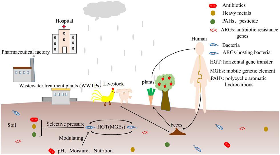
As shown in Figure 1 [7], environmental factors and stressors significantly contribute to the drivers of antibiotic resistance. In the environment, the presence of antibiotic residue has the potential to induce the development of an abundance of antibiotic resistance genes (ARGs) in bacterial colonies and mobile gene elements. Effluent discharge encompasses a broad range of sources, including wastewater treatment plants, excess waste from hospitals, agricultural practices, pollutants, and runoff into soil environments. This impacts soil antibiotic-resistant bacteria (ARB) as it plays an increasingly important role in the evolution and spread of antibiotic resistance in humans and animals. The continuous emergence of soil contamination and

pollution poses new challenges for soil remediation, recovery, and conservation.

Figure 1. Influencing factors of antibiotic resistance genes (ARGs) and antibiotic resistance bacteria (ARB) [7].

Over the past decades, antibiotic consumption has drastically increased [8]. A recent study predicted that global consumption of antibiotics in 2030 could be 200% higher than levels in 2015 in the absence of policy intervention. Raw water from antibiotics industries, effluents from treated wastewater containing antibiotics residues, ARB and ARGs are discharged into the soil through irrigation mechanisms [9]. Reusing treated wastewater effluents in agricultural soil causes serious problems with contamination of ARB and ARGs in agricultural soil [10]. Environmental stressors that amplify antibiotic resistance within soil ecosystems are a significant concern of public health. Tetracycline (tet) and sulfonamide (sul) are antibiotics found within the environment causing the rapid evolution of antibioticresistance genes. Tetracycline and sulfonamide resistance are the most frequently identified ARGs in livestock and agricultural waste found in soil contaminated by antibiotic residues. This has caused an increase in the abundance of ARGs over several decades [8].

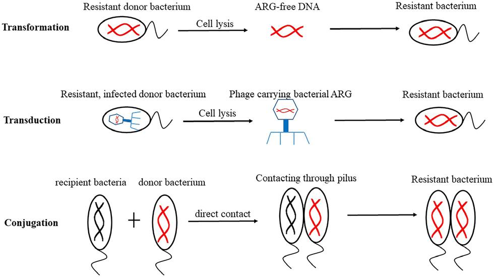
Figure 2. Mechanisms of horizontal gene transfer (HGT) [7].

Figure 2 [7] demonstrates how horizontal and vertical gene transfer mechanisms play a vital role in transferring ARGs and ARB. Existing antibiotics continually exert

selective pressures that have lasting and often permanent changes that affect the bacterial community. This raises the possibility of spontaneous bacterial DNA mutations to create drug resistance and promote horizontal gene transfer (HGT) among bacterial communities. Mobile genetic elements (MGEs), serve microbes by trafficking adaptive traits between species and strains, thereby inducing the uncontrolled spread of ARGs [11].

The study, “Antibiotic Resistance Genes (ARGs) in Agricultural Soils from the Yangtze River Delta, China”, [12] provided valuable insights into the prevalence and diversity of antibiotic resistance genes (ARGs) in agricultural soils. This study highlighted the environmental stressors’ impact on the presence of ARGs, particularly emphasizing the potential role of manure and manure-amended soils in contributing to ARGs in agricultural environments. Most antibiotics used in human medicine have been isolated and originated from soil microorganisms. Therefore, the soil is a potential reservoir of antibiotic-resistance genes and bacteria. The presence of antibiotics in the ground has promoted the development of antibiotic resistance mechanisms in antibiotic-producing and non-producing bacteria [13]. Additionally, the significant impact of farm soil on agricultural practices, particularly the overuse of antibiotics in livestock and crop production, has heightened the proliferation of ARGs and ARB.

A study found that most antibiotic residue in livestock is not fully metabolized and hence is released, together with their transformation products, into the environment along with the feces and urine. In fact, a considerable percentage (30–90%) of the antibiotic administered to a given animal for veterinary purposes can be directly excreted in the urine and feces [14]. Animal manure is commonly applied to soil as organic fertilizer to aid crop production yield and biological properties. Unfortunately, the agronomic application of manure can also lead to the emergence and dissemination of ARB and ARGs in the amended agricultural soil and, subsequently, in the food crops grown for human consumption [15]. This has the potential for contaminated soils in agricultural practices to serve as a carrier of ARGs and ARB to humans and livestock that feed on the crop. For example, Mcr-1 myxin resistance genes were initially found in animals and meat and then detected in food samples and human intestinal flora [16], indicating that ARGs were transmitted from animals to humans. It is also reported that the outbreak of quinolone-resistant Campylobacter infections in the United States is caused by human chicken consumption. Many innovative ideas have been researched to find the best way to remove antibiotics, ARGs, and ARB in the environment. The ultimate goal is to find an environmentally sustainable method that is cost-saving to avoid any secondary pollution from any removal

treatment techniques. Our experiment focuses on one of the most efficient removal methods, biochar, a charcoal-like substance that is made by burning organic material from agricultural and forestry wastes using a specific process to reduce contamination and safely store carbon. As the materials burn, they release little to no contaminating fumes. It is essentially raw biochar, typically produced by heating organic materials such as plant residues or wood in a low-oxygen environment, a process known as pyrolysis. The energy or heat created during pyrolysis can be captured and used as a form of clean energy. Biochar is by far more efficient at converting carbon into a stable form and is more sanitary than other forms of charcoal [8].

Biochar has been proven to be a highly efficient, sustainable absorbent because of its abundant surface functional groups and relatively large surface area. Therefore, it can potentially eliminate or reduce the abundance of antibiotics and pathogenic microorganisms such as ARGs and ARB, in the environment [18]. Using biochar in contaminated soils reduces the bioaccessibility and bioavailability of the contaminants, hence reducing the biological and environmental toxicity. This also reduces contaminants-induced co-selection pressure. Biochar can also repress (HGT) and reduce ARG bacteria hosts, lessening bioavailability, which is favorable for diminishing antibiotic residues in compost and soil [8]. The most common type of biochar is pristine, the original pure form that has not undergone any chemical or physical modifications. It has an efficient enough adsorption mechanism to handle the current pollutants found in contaminated soils in the environment. Modified biochar is designed to improve the adsorption performance of biochar with different physical and chemical modification properties and methods. In modified biochar, the specific surface area was increased by 210.6 % and the adsorption capacity by 87.1 % compared to the pristine biochar. Li et al., stated that the adsorption efficiency of inorganic acid solution-etched biochar increased by 46% more than pristine biochar.

The objective of our study is to investigate whether chemically modified biochar can significantly reduce the abundance of ARB found in environmentally contaminated soil. The hypothesis is that the application of chemically modified biochar with both acidic and alkaline bases will result in a significant reduction of the colony count of antibiotic-resistant bacteria and an increase in the zone of inhibition, indicative of reduced bacterial growth.

2. Methods

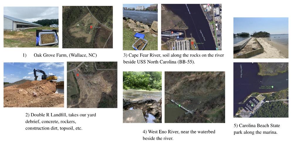
As seen in Figure 3, we collected 15 quarts of surface soil from 5 different areas across North Carolina contaminated with different environmental stressors and environments.

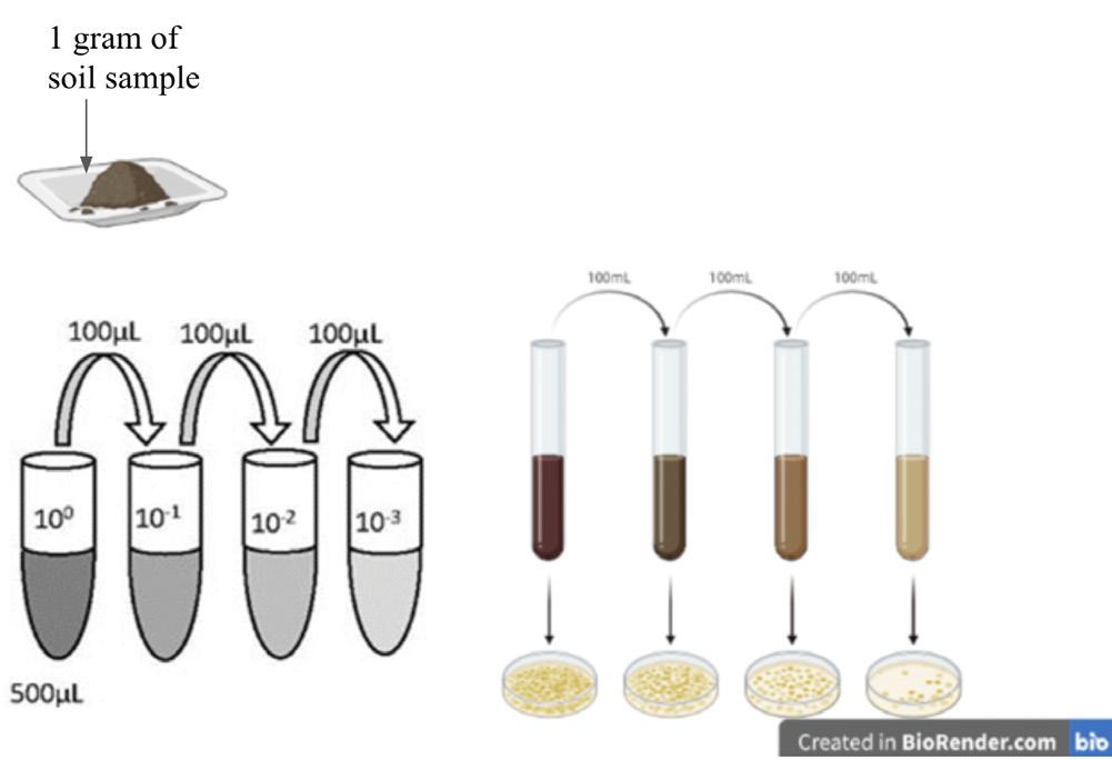
In our preliminary data, as shown in Figure 4 we cultured bacteria isolated from 1 gram of soil samples through a series of serial dilutions in glass test tubes (stock, 10-1, 10-2, and 10-3), using 1 gram of soil as the starting material, then we cultured them onto LB broth agar plates. 40 LB broth plates were divided into two sets, with four different antibiotics disks randomly assigned to each set. The antibiotics disk used were Penicillin, Streptomycin, Neomycin, Tetracycline, Erythromycin, Chloramphenicol, Kanamycin, and Novobiocin [20] which each contained a dosage of either 10 mcg or 30 mcg of antibiotics. Plates were placed in the incubator at 37 °C for 48 hours.

Figure 3. Soil sample collection across North Carolina. (Top) Photos by author, satellite images from Google Earth. (Bottom) Modified from NC General Assembly map.

Figure 4. General methods, culturing of antibioticresistant soil bacteria (created by the author using BioRender).

5. Modified acidic and base biochar treatment methods (diagram created by author).

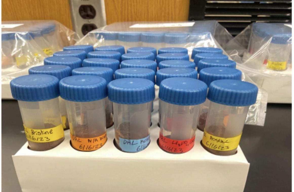
One distinct type of biochar we used was pristine biochar which is derived from softwood and tree trimmings, which we chemically modified using an acidic modification (H3 PO 4) and alkaline modification (KOH) to enhance their physicochemical absorption properties for the biochar [21]. Roughly 50 grams of biochar were soaked in a 30% concentration of H 3 PO 4 and KOH for 24 hours (Figure 5) to have enough for the biochar treatment application (Figure 6). After the biochar was soaked from each solution, it was then carefully separated by draining it through funnel caps using filter paper. To ensure the removal of any residual acid, the biochar was rinsed with distilled water, and this process was repeated three times. Afterwards, the modified biochar was placed in a dryer oven set at 105 °C for an additional 24 hours.

6. Biochar treatment application (image from author).

A total of 200 conical tubes were sampled and were further subdivided into four groups; 1) N/A biochar (no biochar) as the control group 2) pristine biochar that has not gone through any chemical modification 3) acidic modification biochar (H3 PO 4) and 4) alkaline modification biochar (KOH). 40 conical tubes were dedicated to each of the distinct soil sample groups, and within each soil sample group, 10 conical tubes were allocated for each type of biochar sample for duplicates.

Each conical tube was filled with soil up to a volume of 35 mL. Only a small portion, specifically 2% of the recommended amount of biochar, was added to each tube. This amount was determined by the weight of the soil in each tube, with approximately 0.185 grams of biochar added per tube. Setting up this controlled experiment, the biochar’s influence on the soil samples was consistent across all groups. This was to create an environment that promoted the integration and stability of the biochar treatment within the soil samples filled into the conical tubes. This extended exposure to biochar may have influenced the genetic interactions and mobility of the Mobile Genetic Elements (MGEs), reducing the likelihood of horizontal gene transferring (HGT). This approach aimed to provide a more comprehensive evaluation of the long-term impact of biochar in inhibiting HGT within the bacterial community, yielding valuable insights into the treatment’s efficacy before soil samples were retested.

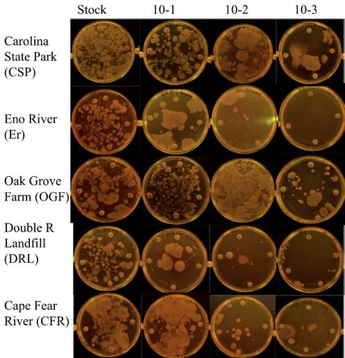
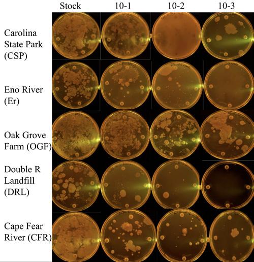
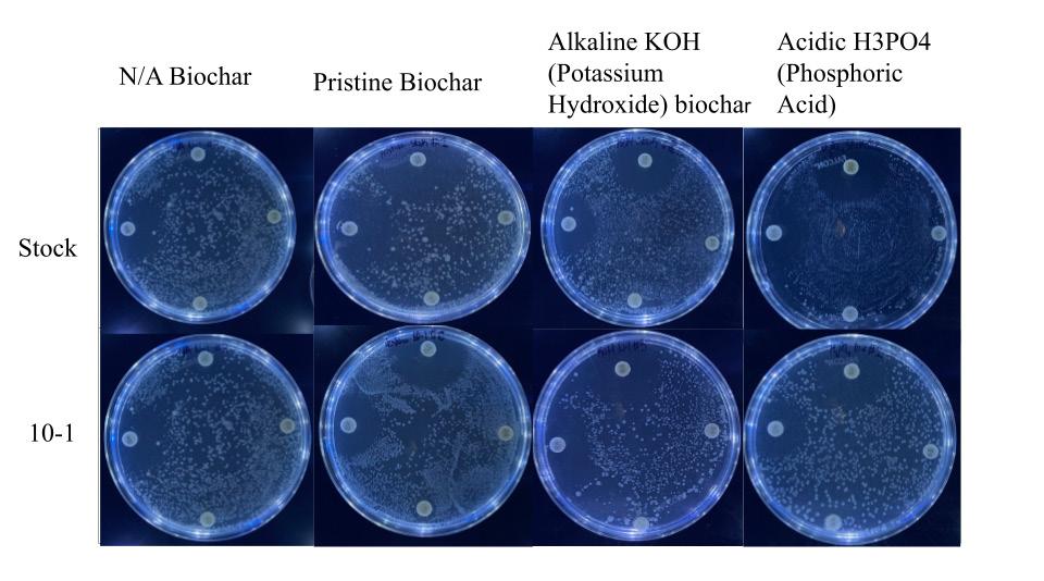
Based on our preliminary results, where duplicates were absent, we obtained data from all soil samples, antibiotic disks, and serial dilution samples. It became evident that the presence of fungi significantly impacted the accuracy of colony counting and the determination of zones of inhibition. Upon visual examination of the images (Figure 7), it was apparent that Oak Grove Farm soil exhibited consistent resistance across all experimental groups, irrespective of the type of antibiotic disk or serial dilution. As a result, this analysis focuses on the decision to prioritize Oak Grove Farm soil and the specific antibiotics to be tested.

Figure

Figure

LB broth agar plates were each inoculated with soil cultures derived from the conical tubes that were initially set up. In response to the insights gained from the preliminary data, we limited our serial dilutions down to only stock and a 10-1 dilution due to limited results in the prior dilutions for 10-2 and 10-3.

To prevent the potential growth of fungal contaminants during plate preparation, we introduced 0.125 grams of antifungal powder into a 500 mL flask that already contained 5 grams of LB broth agar powder and 250 mL of distilled water. This mixture was then autoclaved before pouring the agar plates.

Furthermore, the number of antibiotic disks tested was reduced from eight to four, specifically Penicillin, Tetracycline, Kanamycin, and Novobiocin. This selection was based on the preliminary data, which indicated that these were the least resistant antibiotics, making them the most appropriate candidates for testing on the Oak Grove soil samples. These antibiotics were chosen due to their widespread use in combating bacterial infections.

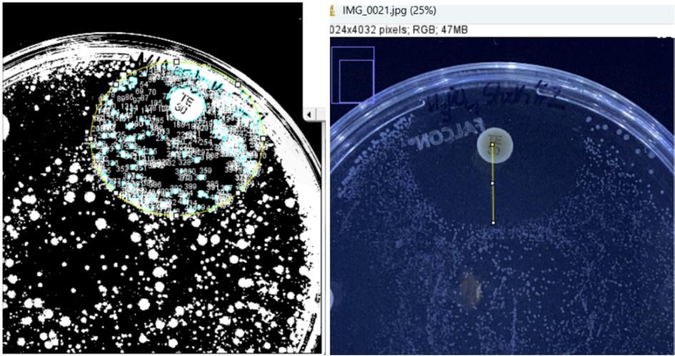
We used Image J software to analyze data as shown in Figure 8. To determine the zone of inhibition (ZOI) of each antibiotic disk, we measured their radius from the center of the antibiotic disk until ZOI ended, using millimeters (mm) as the units of measurement. Before calculating the measurement, we set an appropriate scale from the plate measurement to ensure precise data. Data analysis

could be only conducted for Tetracycline (TE-30) and Kanamycin (K-30) due to the presence of significant ZOI resistance, unlike Penicillin (P-10) and Novobiocin (NB10), which exhibited no resistance across the majority of the data.

For quantifying the resistant bacteria colonies, we used the threshold function within ImageJ to highlight the visibility of the colonies to be able to find a systematic count by circling the boundary of ZOI.

DNA extraction and resistance genes

We conducted a DNA and PCR analysis focusing on three distinct types of antibiotic resistance genes (ARGs), using the DNeasy PowerSoil Pro kit [20] to isolate DNA from the Oak Grove farm soil. Tetracycline G and M genes were chosen due to their relevance to the ongoing testing of tetracycline in our resistant bacteria analysis. We additionally tested the presence of Sulfonamide-1 due to its abundance within the agricultural waste and soil pollution caused by antibiotic residues, which can lead to an increased prevalence of ARGs.

We focused on specific primers that targeted the most abundant ARGs. In particular, we used Tetracycline-G (Tet-G) and Tetracycline-M (Tet-M) due to their relevance to the ongoing testing of tetracycline in our resistant bacteria analysis and Sulfonamide-1 (Sul-1) primers. These primers allowed us to pinpoint and analyze specific ARGs. This contributes to a deeper understanding of antibiotic resistance in agricultural soils influenced by environmental factors, due to their abundance within the agricultural waste and soil pollution caused by antibiotic residues, which can lead to an increased prevalence of ARGs [22][23].

The duplicate PCR reactions were carried out for each gene, while ultrapure water was used as a control to ensure the accuracy of the PCR results. The PCR reaction consisted of 7.5 μL of 10 x PCR Buffer, 8 μL of dNtPS (10 mM), 1.2 μL Taq DNA Polymerase, 67.8 μL double distilled H2O [11]. We used the PCR machine for all three resistance genes primers at an annealing temp of 56 Celsius, 5 min at 95 Celsius for initial denaturation, 40 cycles at 15 seconds at 95 Celsius, 30 seconds of 56 Celsius annealing temperature, 30 seconds at 72 Celsius, an additional 72 Celsius for 5 more min. Later on it was kept at 4 Celsius for 15 hours [24]. Afterwards, we ran our primers through our gel electrophoresis which consisted of SYBR Premix Ex TaqTM (TaKaRa), 4.6 μL of double-distilled water, 0.3 mL of the 50× ROX reference dye, 0.3 μL of the forward primer (10 mM), 0.3 μL of the reverse primer (10 mM) and 2 μL of the template DNA to identify whether or not there was a presence of our resistance genes from our soil.

These ARG analyses were tested on both no biochar (N/A biochar) and acid-modified biochar. The choice to include the acidic biochar was due to earlier results, which

Figure 7. Antibiotic Resistance Profiling- Preliminary data (diagram created by author)

Figure 8. Quantitative Analysis of Bacterial Colonies and Inhibition Zone (Created by the author using ImageJ software).

Figure 9. Antibiotic Resistance Profiling, inoculating the testing samples with bacterial cultures derived from soil colonies collected at Oak Grove Farm. (diagram created by author).

indicated the most efficiency in reducing the abundance of ARB. These selected samples allowed for a focused examination of the impact of biochar modifications on ARGs associated with soil, particularly in the context of agricultural waste and its contribution to soil pollution.

3. Results

Antibiotic Resistance Profiling

For the preliminary data presented in Figure 7, we conducted tests on two sets of plates for all soil samples. Each set contained eight antibiotic disks divided into four identical antibiotic disks for each group, ranging from stock to 10-3 dilutions. As shown in Figure 9, after introducing the antifungal treatment, we were able to accurately count colony numbers and measure zones of inhibition using only four antibiotics consistently positioned in the same location.

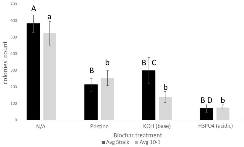
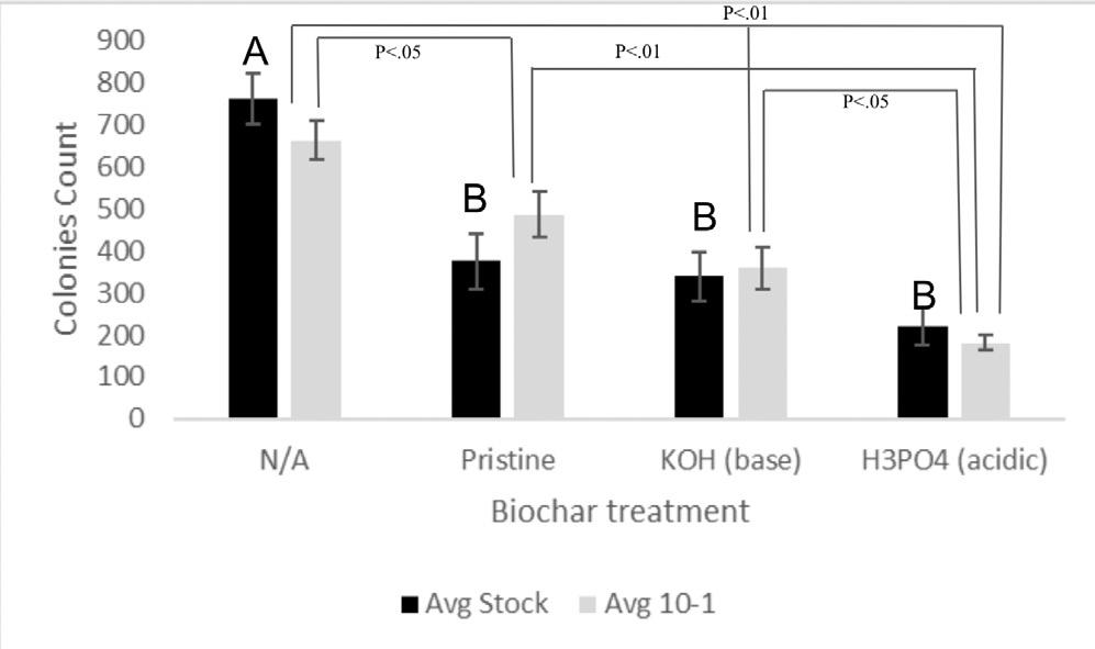
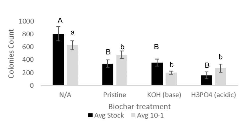
Antibiotic resistance profiling exhibited that modified biochar was significant (p<0.01) in reducing the number of colony counts for Tetracycline (TE-30), Kanamycin (K-30), and Novobiocin (NB-10) antibiotics, for both Stock and 10-1 groups (Fig 10, Fig 11, Fig 13). For the TE30 Stock, the alkaline biochar treatment was significantly better compared to the acidic treatment (p < 0.05). For the Penicillin (P-10) antibiotic disk, modified biochar also significantly reduced the number of colony counts compared to N/A biochar in both Stock and 10-1 groups (Fig 12). The results were intriguing, showing consistent significance (p < 0.01) for P-10 stock, yet P-10 10-1 remained significant but had a p-value of p < 0.05 when compared to the N/A biochar treatment as opposed to the

acidic biochar treatment. Pristine and alkaline biochar treatments were also significantly better than the acidic biochar treatment, with p-values of p < 0.01 and p < 0.05 for all four drugs.

Fig 10. Tetryacline (TE-30). The addition of biochar reduces the number of colonies. (ANOVA, F=16.69, 18.1, DF=3, P< 0.001, stock and 10-1 respectively) Capital letters indicate differences between stock solutions. Lower case letters indicate differences between 10-1 dilution. Error bars represent St.Error. AvB p<.01. CvD p<.05

Fig 11. Kanamycin (K-30). The addition of biochar reduces the number of colonies. (ANOVA, F=29.57, 38.3, DF = 3, P< 0.001, stock and 10-1 respectively) Capital letters indicate differences between stock solutions. Lower case letters indicate differences between 10-1 dilution. Error bars represent St.Error. AvB p<.01

Fig 12. Penicillin (P-10). The addition of biochar reduces the number of colonies. (ANOVA, F=16.91, 21.3, DF=3, P< 0.001, stock and 10-1 respectively) Capital letters indicate differences between stock solutions. Error bars represent St.Error. AvB p<.01.

Fig 13. Novobiocin (NB-10). The addition of biochar reduces the number of colonies. (ANOVA, F=12.65, 38.3, DF=3, P< 0.001, stock and 10-1 respectively) Capital letters indicate differences between stock solutions. Lower case letters indicate differences between 10-1 dilution. Error bars represent St.Error. AvB p<.01.

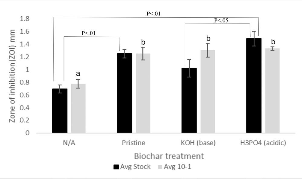
Additionally, the results from the antibiotic resistance profiling indicate a significant increase in the zone of inhibition with the addition of modified biochar compared to N/A biochar, specifically in the Tetracycline (T-30) and Kanamycin (K-30) 10-1 groups, consistently achieving a p-value of p < 0.01 (Fig 14 and Fig 15).

However, the N/A biochar treatment was not significant compared to alkaline biochar treatment, but it was significant when compared to the acidic biochar treatment for both T-30 and K-30 stock.

Fig 14. Tetryacline (TE-30). The addition of biochar increases the zone of inhibition. (ANOVA, F=9.84, 15.06, DF =3, P< 0.001, stock and 10-1 respectively). Lower case letters indicate differences between 10-1 dilution. Error bars represent St.Error. AvB p<.01.

Fig 15. Kanamycin (K-30). The addition of biochar increases the zone of inhibition. (ANOVA, F=11.48, 9.79, DF =3, P< 0.001, stock and 10-1 respectively). Lower case letters indicate differences between 10-1 dilution. Error bars represent St.Error. AvB p<.01.

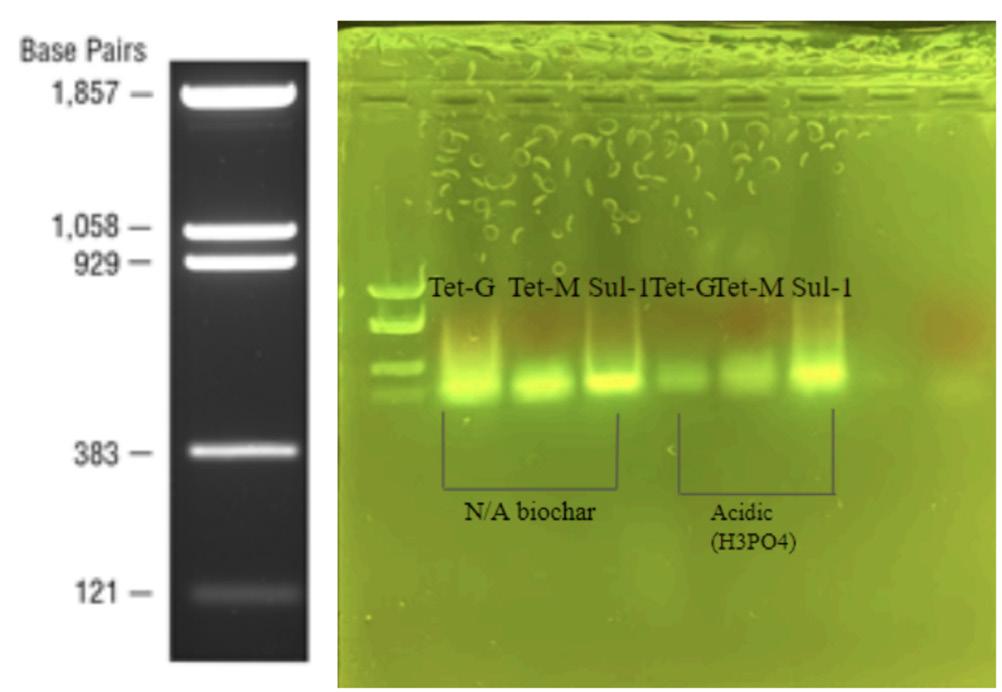
After running our gel electrophoresis, the data analysis revealed the presence of all three antibiotic-resistance genes in the N/A biochar and acidic biochar samples (Fig 16). To determine the size of the bands, a pBR322 DNA-BstNI Digest was utilized as a ladder for base pair differentiation along with our primers.

Figure 16. DNA analysis of antibiotic resistance genes (Tet-G, Amplicon Size (bp) = 133, Tet-M, Amplicon Size (bp) = 171, sul-1T, Amplicon Size (bp) = 158)

4. Conclusion and Future Directions

This experiment demonstrated that modified biochar significantly reduces the abundance of antibioticresistant bacteria (ARB) found in the contaminated soil, focusing on agricultural environments. Based on our preliminary data, results indicated that Oak Grove Farm consistently exhibited elevated resistance levels and smaller zones of inhibition across all tested antibiotics. Thus, this led to a focus on Oak Grove Farm, testing various biochar treatment groups.

Penicillin (P-10) and Novobiocin (NB-10) consistently proved to be resistant to every biochar treatment that increases the zone of inhibition (ZOI), despite the fact that Penicillin was considered the “first wonder drug”, being one of the most commonly used antibiotics globally for numerous bacterial infections. Additionally, Novobiocin is commonly used as an alternative to penicillins, against penicillin-resistant infection, however, its decreasing effectiveness over time exemplifies the impact of evolution on its resistance to both antibiotics. Overall, after a comprehensive analysis of the data and graphs, modified biochar significantly reduced the abundance of ARB. This is observed by the colony counts and ZOI measurements, which are indicative of bacterial growth and resistant bacterial colonies.

Among the various biochar treatments applied, acidic biochar treatment consistently outperformed the others, demonstrating significant results across all graphical representations. This observation strongly suggests that modified biochar can significantly enhance adsorption capacity and mitigate the co-selection pressure exerted by contaminants of antibiotic residues. This can help repress (HGT) and reduce the presence of antibioticresistant genes (ARGs) within bacterial hosts, thus further reducing bioavailability.

These results are significant, as modified biochar

appears to be a promising solution for future environmental sustainability practices. Modified biochar is also a cost-effective and environmentally friendly approach that has the potential to prevent secondary pollution resulting commonly from alternative removal techniques such as ozonation. This approach can be incorporated into routine agricultural practices and livestock management to reduce the emergence and dissemination of ARB and ARGs within agricultural soils and the environment, which are recognized reservoirs for antibiotic residues. Ultimately, this has significant implications for food crops grown for human consumption, considering the potential for ARGs to persist due to evolutionary processes.

However, the consistency observed in all our data remained until the analysis of DNA revealed the presence of antibiotic resistance genes (ARGs) in both N/A and acidic biochar samples. This prompts more questions regarding whether, despite the significant reduction in the abundance of antibiotic-resistant bacteria (ARB) achieved by modifying biochar in contaminated soil, there may still be a lingering presence of mobile genetic elements within bacterial communities, still potentially facilitating ongoing horizontal gene transfer within the soil environment. This aspect of our results provokes future discussion and research into alternative methods of modification and techniques for effectively mitigating both antibiotic resistance and the persistence of antibiotic-resistance genes. In the future, there are several promising avenues for future research. Due to time constraints and availability, we were not able to complete the culturing of all soil samples, which would have entailed 400 plates to accommodate both stock and 10-₁ dilutions, twice that amount of antibiotic disk tests remain unexplored in our final results, despite their inclusion in our preliminary data.

Looking ahead our objective is to expand the experiment to the rest of our soil samples and antibiotics. Specifically, we assess whether significant differences exist in comparison to our findings for Oak Grove Farm soil. Notably, we have already prepared the necessary experimental setups for the remaining conical tubes to carry out these tests.

In addition, further researching our soil samples, we want to look closer at the 16S rRNA gene sequencing antibiotic resistance genes within the soil. Previous research has shown that tetracycline (tet) genes in soils worldwide varied between 10-6 to 10-2 gene copies per 16S rRNA gene copies [22] [23]. Given that the sul and tet resistance genes were often detected in manure or manureamended soils [12], application of manure fertilizer and wastewater irrigation could be the main anthropogenic sources of ARGs for agricultural soil environments [24]. However, current limitations in equipment prevented

us from conducting this sequencing. Nevertheless, the potential for this research to provide valuable insights in the future.

This study offers numerous directions for future considerations. Researching further into soil remediation, recovery, and conservation on a broader scale in an environmental context has the potential to expand understanding of antibiotic resistance and its mitigation in soil environments.

5. Acknowledgments

Thank you to my mentor Dr. Mallory for always believing in me and her constant guidance supporting me throughout my research project. Also thank you to Dr. Monahan, Dr. Sheck, Dr. Maitê, Glaxo lab, my dad, who has always been my biggest advocate, Keith Hairr, the farmer who gave me his soil, and my Research in Biology peers with whom I made lifelong friends and made this experience enjoyable. I couldn’t have done this without all their support, truly.

Funding: Glaxo, NCSSM Foundation, Burroughs Wellcome Fund

6. References

[1] Llor, C. and Bjerrum, L. (2014). Antimicrobial resistance: Risk associated with antibiotic overuse and initiatives to reduce the problem. Therapeutic Advances in Drug Safety, 5(6), 229–241. https://www.ncbi.nlm.nih. gov/pmc/articles/PMC4232501/

[2] Okeke, I. N., Laxminarayan, R., Bhutta, Z. A., Duse, A. G., Jenkins, P., O’Brien, T. F., Pablos-Mendez, A., and Klugman, K. P. (2005). Antimicrobial resistance in developing countries. Part I: recent trends and current status. The Lancet. Infectious Diseases, 5(8), 481–493. https://www.sciencedirect.com/science/article/pii/ S1473309905701894

[3] Denyer Willis, L. and Chandler, C. (2019). Quick fix for care, productivity, hygiene and inequality: reframing the entrenched problem of antibiotic overuse. BMJ Global Health, 4(4), e001590. https://www.ncbi.nlm.nih.gov/ pmc/articles/PMC6703303/

[4] CDC. (2019, March 8). Antibiotic / Antimicrobial Resistance. Centers for Disease Control and Prevention. https://www.cdc.gov/drugresistance/index.html

[5] Nathan, C. (2004). Antibiotics at the crossroads. Nature, 431(7011), 899–902. https://www.nature.com/ articles/431899a

[6] Gould, I. M., and Bal, A. M. (2013). New antibiotic agents in the pipeline and how they can help overcome microbial resistance. Virulence, 4(2), 185–191. https://doi. org/10.4161/viru.22507

[7] Front Microbiol. (2022). 13: 976657. NIH. https://www. ncbi.nlm.nih.gov/pmc/articles/PMC9539525/figure/fig1/

[8] Zhuang, M., Achmon, Y., Cao, Y., Liang, X., Chen, L., Wang, H., Siame, B. A., and Leung, K. Y. (2021). Distribution of antibiotic resistance genes in the environment. Environmental Pollution, 285, 117402. https://www.sciencedirect.com/science/article/pii/ S0269749121009842

[9] Guo, Y., Liu, M., Liu, L., Liu, X., Chen, H.-H., and Yang, J. (2018). The antibiotic resistome of free-living and particleattached bacteria under a reservoir cyanobacterial bloom. 117, 107–115. https://www.sciencedirect.com/science/ article/pii/S0160412018300886

[10] Kumar, A. and Pal, D. (2018). Antibiotic resistance and wastewater: Correlation, impact and critical human health challenges. Journal of Environmental Chemical Engineering, 6(1), 52–58. https://www.sciencedirect. com/science/article/pii/S2213343717306176

[11] Chen, H. and Zhang, M. (2013). Occurrence and removal of antibiotic resistance genes in municipal wastewater and rural domestic sewage treatment systems in eastern China. Environment International, 55, 9–14. https://www.sciencedirect.com/science/article/pii/ S0160412013000391

[12] Qiao, M., Ying, G.-G., Singer, A. C., and Zhu, Y.-G. (2018). Review of antibiotic resistance in China and its environment. Environment International, 110, 160–172. https://www.sciencedirect.com/science/article/pii/ S0160412017312321

[13] Aminov, R. I. (2009). The role of antibiotics and antibiotic resistance in nature. Environmental Microbiology, 11(12), 2970–2988. https://pubmed.ncbi. nlm.nih.gov/19601960/

[14] Kumar, K., C. Gupta, S., Chander, Y., and Singh, A. K. (2005, January 1). Antibiotic Use in Agriculture and Its Impact on the Terrestrial Environment. ScienceDirect; Academic Press. https://www.ncbi.nlm.nih.gov/pmc/ articles/PMC3587239/

[15] Peng, S.-A., Feng, Y., Wang, Y., Guo, X., Chu, H., and Lin, X. (2017). Prevalence of antibiotic resistance genes in soils after continually applied with different manure for 30 years. Journal of Hazardous Materials, 340, 16–25. https://pubmed.ncbi.nlm.nih.gov/28711829

[16] Han, B., Ma, L., Yu, Q., Yang, J., Su, W., Hilal, M. G., Li, X., Zhang, S., and Li, H. (2016). The source, fate and prospect of antibiotic resistance genes in soil: A review. Frontiers in Microbiology, 13. https://www.ncbi.nlm.nih. gov/pmc/articles/PMC9539525/

[17] Holt, J., Yost, M., Creech, E., McAvoy, D., and Allen, N. (2021, April). Biochar Impacts on Crop Yield and Soil Water Availability. extension.usu.edu. https://extension. usu.edu/crops/research/biochar-impacts-on-crop-yieldand-soil-water-availability

[18] Sanganyado, E. and Gwenzi, W. (2019). Antibiotic resistance in drinking water systems: Occurrence, removal, and human health risks. Science of the Total Environment, 669, 785–797. https://pubmed.ncbi.nlm. nih.gov/30897437/

[19] Li, S., Zhang, C., Li, F., Hua, T., Zhou, Q., and Ho, S.-H. (2021). Technologies towards antibiotic resistance genes (ARGs) removal from aquatic environment: A critical review. Journal of Hazardous Materials, 411, 125148. https://www.sciencedirect.com/science/article/pii/ S0304389421001114

[20] Carolina Biological. (2019). https://www.carolina. com/

[21] Wu, N., Qiao, M., Zhang, B., Cheng, W.-D., and Zhu, Y.-G. (2010). Abundance and Diversity of Tetracycline Resistance Genes in Soils Adjacent to Representative Swine Feedlots in China. Environmental Science and Technology, 44(18), 6933–6939. https://doi.org/10.1021/ es1007802

[22] Ji, X., Shen, Q., Liu, F., Ma, J., Xu, G., Wang, Y., and Wu, M. (2012). Antibiotic resistance gene abundances associated with antibiotics and heavy metals in animal manures and agricultural soils adjacent to feedlots in Shanghai; China. Journal of Hazardous Materials, 235236. https://www.sciencedirect.com/science/article/pii/ S0304389412007716

[23] Wang, S., Gao, B., Zimmerman, A. R., Li, Y., Ma, L., Harris, W. G., and Migliaccio, K. W. (2015). Removal of arsenic by magnetic biochar prepared from pinewood and natural hematite. Bioresource Technology, 175, 391–395. https://www.sciencedirect.com/science/article/pii/ S0960852414015363

[24] Luo, Y., Mao, D., Rysz, M., Zhou, Q., Zhang, H., Xu, L., and J. J. Alvarez, P. (2010b). Trends in Antibiotic Resistance Genes Occurrence in the Haihe River, China. Environmental Science and Technology, 44(19), 7220–7225. https://doi.org/10.1021/es100233w

[25] Bartholomew, M.J., Hollinger, K., and Vose, D. (2003) Characterizing the risk of antimicrobial use in food animals: fluoroquinolone-resistant campylobacter from consumption of chicken. Microbial Food Safety in Animal Agriculture: Current Topics. Ames, IA: Iowa State Press, 293–301.

[26] Godwin, P. M., Pan, Y., Xiao, H., and Afzal, M. T. (2019). Progress in Preparation and Application of Modified Biochar for Improving Heavy Metal Ion Removal From Wastewater. Journal of Bioresources and Bioproducts, 4(1), 31-42. https://doi.org/10.21967/jbb.v4i1.180

[27] Sun, J., Jin, L., He, T., Wei, Z., Liu, X., Zhu, L., and Li, X. (2020). Antibiotic resistance genes (ARGs) in agricultural soils from the Yangtze River Delta, China. Science of the Total Environment, 740, 140001. https://www.sciencedirect.com/science/article/pii/ S004896972033521X

[28] Singer, A. C., Shaw, H., Rhodes, V., and Hart, A. (2016). Review of Antimicrobial Resistance in the Environment and Its Relevance to Environmental Regulators. Frontiers in Microbiology, 7. https://www.frontiersin.org/ articles/10.3389/fmicb.2016.01728/full

[29] Zhou, Z., Liu, J., Zeng, H., Zhang, T., and Chen, X. (2020). How does soil pollution risk perception affect farmers’ pro-environmental behavior? The role of income level. Journal of Environmental Management, 270, 110806. https://www.sciencedirect.com/science/article/ pii/S0301479720307374

IDENTIFICATION OF SINGLE-NUCLEOTIDE POLYMORPHISMS

RELATED TO THE PHENOTYPIC EXPRESSION OF DROUGHT TOLERANCE IN ORYZA SATIVA

Reva Kumar

Abstract

Environmental stressors have contributed to the depletion of crop yield for major crops like rice due to climate change. Characteristics such as drought tolerance are critical indicators of stress. We identified genes associated with drought tolerance using several quantitative techniques. These include quantitative trait loci (QTL) analyses and genome-wide association studies (GWAS). The QTL analyses used a cross between Curinga and O. rufipogon. The GWAS study looked at a dataset of 413 rice varieties and approximately 44,000 single nucleotide polymorphisms (SNPs) on each of the species. The dataset contained 37 phenotypes. The goal was to use a kinship matrix as a correction for a GWAS analysis on a specified phenotype and to identify the most significant SNPs. We selected four major phenotypes possibly correlated with drought tolerance: plant height, seed length to width ratio, amylose content, and protein content. The analyses identified several genes local to the SNP region using a genome browser. Current work involves relating phenotype expression under environmental stimuli to orthologous genes in model plants like Arabidopsis thaliana and Zea mays. This study aims to use these genes in understanding the relationship between drought tolerance and gene presence/ expression in rice. This study will continue to identify species with genetic expressions correlating to high drought tolerance, with further applications to finding species that can be cross-bred to produce drought tolerant species of rice.

1. Introduction

Drought occurs during an extended imbalance between precipitation and evaporation. With the increasing severity of climate change, historically dry areas are likely to have increased drought occurrences in the coming years. From 2015-2021, extreme dry and wet events in the U.S. occurred four times per year, versus three times in the 15 preceding years. It is predicted that over 50% of the world’s arable land will be affected by drought in the year 2050 [1]. This is a major concern for agriculture. Rice is considered a key crop in global food security, since it is the primary nutrient source for more than three billion people [2]. However, rice is one of the most drought-susceptible plants because it cannot take up much water due to its small root system [3].

As the global population continues to grow, the demand for technologies that enhance crop yield has risen. Environmental stressors, including drought, have contributed to the depletion of crop yield. For rice, there was a 25.4% decline from 1980 to 2017 [4]. Critical mitigation of rice drought tolerance is needed to maintain global food security.

Because of the drastic effects drought has on plant growth, understanding the genetic expression of rice during drought is crucial for the mitigation of drought stress. Drought tolerance is composed of morphological

adaptations, so this study focuses on the phenotypic expression of some morphological features.

Rice is cultivated globally and has a genome with 12 chromosomes encompassing 430 Mbp (mega base pairs). Past literature has identified genes in rice correlated with drought tolerance, but this approach seeks to use several quantitative techniques, including Quantitative Trait Loci (QTL) analyses and Genome Wide Association Studies (GWAS), to identify genes associated with phenotypes related to crop yield. This paper also uses these two quantitative techniques to compare genes observed for plant height, and this is a unique approach compared to past studies [6].

Drought stress is the result of a long-term period of low soil moisture content accompanied by a continuous loss of water through evaporation and transpiration [7]. Thus, to understand drought stress, it is imperative to understand the morphological, physiological, and biochemical responses of rice to stress. Since phenotypes are mainly observed through morphological responses [5], this paper observes how decreased plant height and a reduced number of tillers, also known as shoots, could denote poor yield. Poor yield is determined by attributes such as impaired assimilate partitioning, reduced grain filling, grain weight and size, and death of the plant. Figure 1 shows how drought stress could contribute to morphological responses and correspond to poor yield.

Though physiological and biochemical responses were not as heavily studied, all three response types could result in poor yield attributes [5]. Furthermore, morphological responses could be related to shoot development and characteristics during early development.

Figure 1: Drought stress influence on morphological, physiological, and biochemical responses of rice [5]

Various studies have found that other than morphological attributes denoting poor yield, there could be traits such as amylose and protein content that indicate poor yield. Insufficient water supply could lead to the reduction of carbohydrate synthesis in crops and lower grain and protein yield [8].

Overall, this study analyzes phenotypes with known correlations to environmental stimuli to observe how morphological changes due to drought tolerance may be the result of gene functions. Selected genes with quantitative statistical significance were observed using genome browsers to find gene functions and drought tolerant traits. This study responded to three main research questions:

1. Are there genes expressed in rice that are influenced by phenotypes related to drought?

2. Can the functions of these genes correlate to drought tolerance?

3. How can these genes be used to identify orthologous genes in other species and draw conclusions for drought tolerance?

2. Computational Approach/Methods

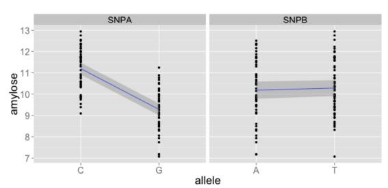
This study used two main quantitative techniques for identifying loci. The first technique is a GenomeWide Association Study (GWAS). Generally, GWAS work to find genes that are associated with phenotypes across the whole genome [9]. Association mapping in this study identifies single-nucleotide polymorphisms (SNPs), or genomic variants at a single location within one nucleotide [10]. If there is a non-zero slope along

the association between observed data for the same trait, there is an association between a SNP allele and a phenotype. An example of this association is shown in Figure 2.

Figure 2: The non-zero slope for SNPA shows that it is significant because there is a correlation between the allele present and the phenotype observed. The flat correlation between the alleles on SNPB shows that it is an insignificant SNP. The y-axis corresponds to relative quantities of amylose, rather than specified quantities with units. In this case, two SNPs for amylose were portrayed, with SNPA showing the presence of C versus G yielded higher amylose content.

We used a GWAS model with a dataset including 413 rice varieties from 82 countries and 44,000 genetic mutations, or SNPs on each type of rice. Although there are around 500,000 SNPs among rice varieties, due to linkage disequilibrium closely linked SNPs have high correlation. Thus, the majority of known SNPs are not necessary for the study. The goal of the GWAS was to identify loci that may indicate the expression of a particular trait. The dataset includes 37 phenotypes, but those that were most significantly linked to drought tolerance were studied, including: plant height, seed length to width ratio, amylose content, and protein content.

Since the dataset was so large, a kinship matrix was used to adjust for population structure, assuming kinship from the observed genotypic data. A kinship matrix displays the genetic relatedness of organisms, with values representing genetic similarity ranging from 0 to 1 (1 as identical organisms, 0 as unrelated organisms). The kinship matrix in this method is estimated from the SNPs and data given, since the pedigree of the species is unknown. A LOD-score, also known as logarithm of odds, was used to estimate the genetic relatedness of a marker and an expressed trait. The LOD-score threshold for this data was 5.85, which is significant for plants [11]. After including a kinship matrix in the GWAS, significant SNPs were chosen. The three SNPs with the highest LOD scores at that location were identified as most significant. In this study, a specific type of LOD score was used that used a -log(P) as normalization for the dataset. There is a 95% certainty in this study, with a -log(P) used to normalize the data for association rather than probability

of association by chance [12].

The second major quantitative technique that was used is a Quantitative Trait Loci (QTL) Analysis. QTL analyses work to identify molecular markers associated with phenotypes, rather than genes or purely genetic loci [6]. The QTL analysis was conducted on a cross-inbred population of Curinga x Oryza rufipogon. For the QTL data, the dataset was rather small, incorporating phenotypes of flow, height, tillers, panicles, and pericarp. Panicles refer to branching clusters of rice and perciparp refers to the layer surrounding the ovary wall of a plant’s seed. Based on the category ”Morphological Responses” from Figure 1, tillers and height were chosen as proxies for drought.

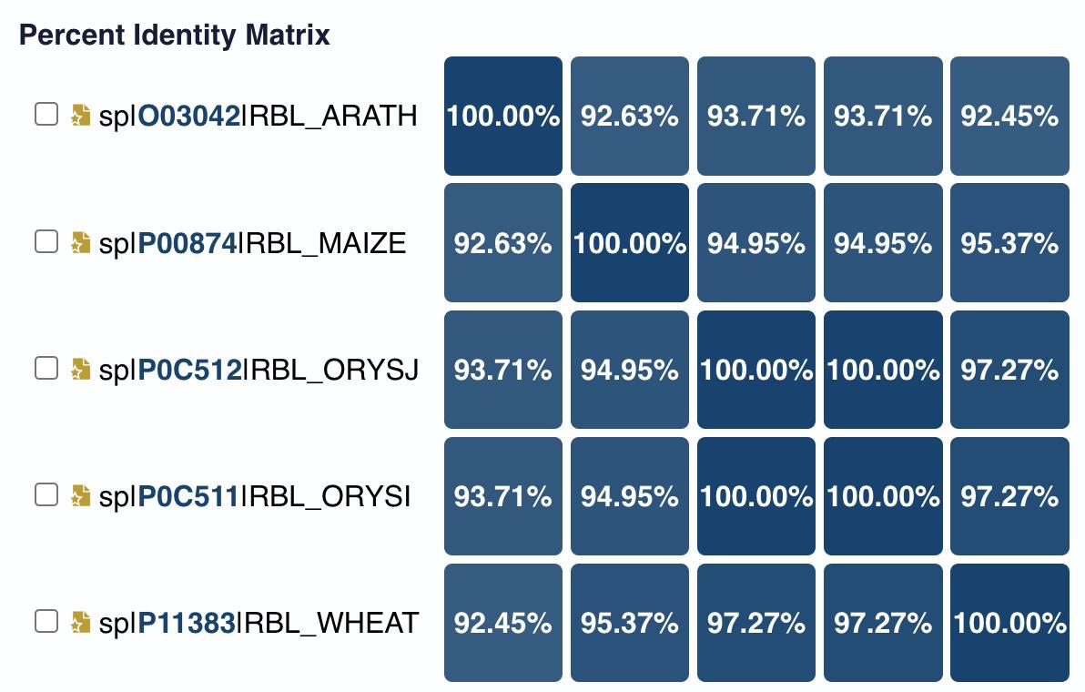
Using publicly available rice and plant genome browsers, genes were identified that were nearest to the identified loci. The Rice Genome Annotation Project (RGAP) Browser from the University of Georgia shows all 12 chromosomes with markers along all base pairs. Rice loci were identified, as well as the best orthologous genes/proteins in Arabidopsis thaliana (thale cress) and Zea mays (maize). These were two plants that had genetic similarities of 93.71% and 94.95% to rice, respectively, as seen in Figure 3. Although Triticum aestivum (wheat) had a higher genetic relatedness, it was easier to find orthologous genes in Arabidopsis thaliana and Zea mays because their genomes have been mapped extensively (especially Arabidopsis thaliana). The RGAP individual gene pages show gene ontologies (GO) and their accessions. These include the biological processes that are known as gene functions.

Figure 3: The percent genetic relatedness between Arabidopsis thaliana, Zea mays, Oryza sativa japonica, Oryza sativa indica and Triticum aestivum. These are listed vertically, where the japonica and indica species have 100% relatedness. This image was produced by creating a percent identity matrix on UniProt.

While the RGAP browser did not have extensive details on the ontologies, UniProt, a web-accessed resource, did, and was used to search for known genes from the QTL and GWAS studies and identify details about the proteins

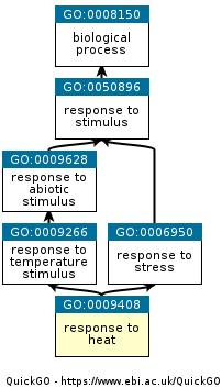
encoded in those genes and their functions. The main ontologies that aligned with the goals of the study were those related to biological processes marking responses to environmental external stimuli, as seen in Figure 4. Response to general environmental stress and heat/ temperature stimuli ontologies were found.

Figure 4: Gene Ontology accessions with responses to heat stimuli. This image shows blue boxes as biological processes with the black arrows pointing to possible processes that are influenced. The GO accession numbers refer to different possible processes in the rice genes. Each specific number classification is not significant, but the processes they entail are. This diagram was produced by the European Bioinformatics Institute’s gene ontology browser.

While not every gene had extensive information about it, general conclusions were drawn from gene ontologies on how those genes could be affected by external stimuli, with a focus on drought and heat.

3. Results and Discussion

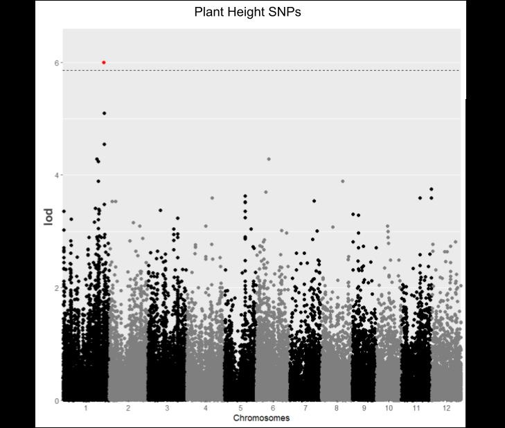
For the plant height phenotype studied using a GWAS, one significant SNP was found, with a LOD score of 5.99 and location of 38111539 bp on Chromosome 1, as shown in Figure 5.

Figure 5: This shows the GWAS analysis adjusted with a kinship matrix for plant height, identifying one significant SNP as shown in red.

The three nearest loci were LOC Os01g65650, LOC Os01g65640, and LOC Os01g65660, as seen in Figure 6. LOC refers to an identified loci, Os refers to Oryza sativa, the number 01 refers to the chromosome, and the remaining numbers denote the number gene it is.

Figure 6: a) Genome Browser showing SNP on the genome with nearby loci. b) LOC Os01g65650 shown on the genome.

LOC Os01g65650 was observed as a protein-coding gene but little information was available. An orthologous Arabidopsis thaliana gene was identified as AT1G72180. The gene ontology showed the purpose of the gene is to mediate nitrate uptake and to regulate the shoot system development and response to osmotic stress. It is possible that this result – plant height correlated with shoot system regulation – could be used as a proxy to results with tillers. This gene is also expressed heavily during the growth stages of the plant. Growth stages involving the root system may be correlated to plant height expression. Since the small root system of rice contributes to its high susceptibility to drought, this gene could be

studied more extensively in the future to understand correlations between plant root development and height. Furthermore, osmotic stress could directly be related to drought influence, due to the imbalance in salinity and important ions in the cell [13]. There is an emphasis on this gene’s functionality with shoot development, a key indicator of healthy plant growth under sufficient hydration.

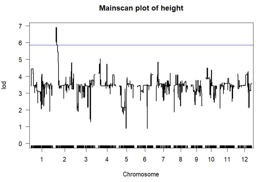
For observing the plant height phenotype using QTL analysis, a mainscan plot was produced, as shown in Figure 7. The most significant QTL identified was one at Chromosome 2 and position 3.12 cM, with a LOD score of 6.91. 3.12 is the location in cM (centimorgans), so conversion to base pairs found the location as 842400 bp. This was observed in the rice genome browsers (Figure 8).

Figure 7: Mainscan plot showing the QTLs for height along the genome, with a peak at Chromosome 2 indicating a high LOD score and therefore high statistical significance. The blue line represents the LOD threshold of 5.85.

Figure 8: Rice Genome Browser showing location of Chromosome 2 at 842 kbp.

The QTL was observed in gene LOC Os02g02410, a DnaK family protein with an orthologous gene in Arabidopsis thaliana as AT5G42020. A DnaK protein expressed in chromosome 3 was also found, with possible proteins encoding for heat stress. It acts as a protein binder in response to heat stress, and there is a possibility that this DnaK protein could be used to target other environmental stressors, like drought. Other GO accessions not identified in the genes so far were 0009628 and 0006950, which could correspond to drought stress response. Further research may include identifying these accessions in QTLs and finding more phenotypes associated with these biological processes. Furthermore, a GO accession of GO:0009408 was present, which is related to heat stimuli response. Using the rice expression

database, UniProt was used to identify another protein in the gene, Q6Z7B0, a kDa protein involved in the control of seed storage proteins during seed maturation. Due to the nature of the GWAS-identified plant height gene as a protein-coding gene, it is assumed that this gene has a purpose in coding for endoplasmic reticulum stress and therefore is crucial to the seed development. Additionally, both are expressed after flowering during seed development, not in mature seeds. Drought can decrease the quality of seeds during early development, thus contributing to poor plant growth [14]. No QTLs were identified for tillers, an additional possible indicator of drought tolerance. This is possibly due to the lack of data for this phenotype.

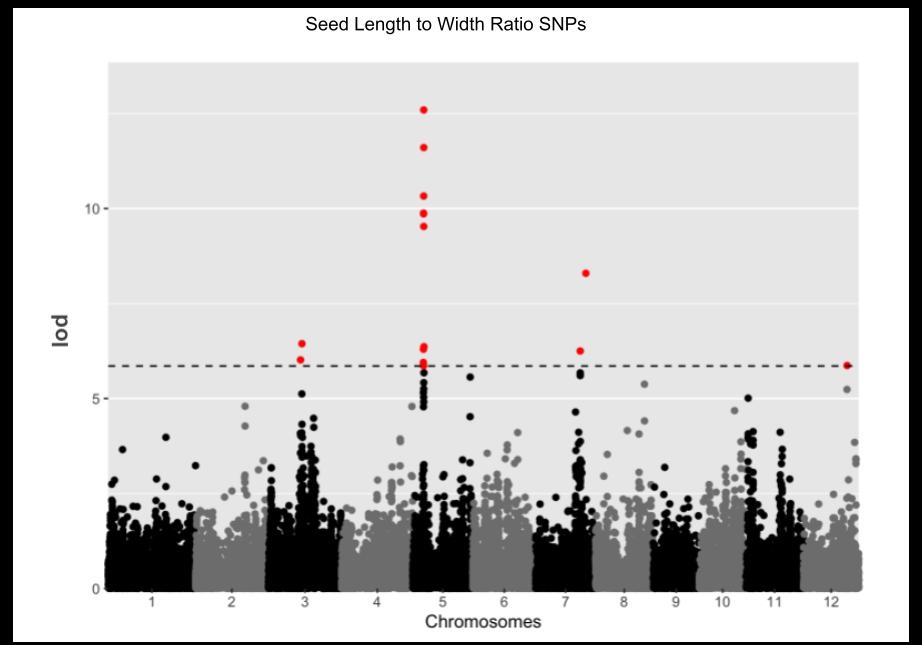
Other phenotypes were observed using GWAS. Seed length to width ratio was observed having a significant SNP at Chromosome 5 and location 5425317 bp, with LOD score 12.59, as seen in Figure 9. LOC Os05g09550 was the gene that contained this SNP, and is a Der-1-like family containing protein. It is involved in the degradation of proteins in the endoplasmic reticulum, which is similar to the traits observed from the plant height loci.

Figure 9: This shows the GWAS analysis adjusted with a kinship matrix for seed length to width ratio. There is a peak in significant SNPs at chromosome 5, and these genes are all close to each other.

The amylose content phenotype GWAS analysis suggested the gene LOC Os06g04200, a starch synthase with molecular functions in protein binding and metabolism. Since these are traits mainly correlated with plant regulation and the synthesis of vital nutrients, these could be compromised under drought stress, like they have been in sweet potato [15].

Finally, the protein content phenotype GWAS analysis suggested the gene LOC Os06g09880, as seen in Figure 10, contributes to major reproductive and embryonic development. Though this is different from the protein binding and metabolism processes seen with the other phenotypes, it still deals with seed development, suggesting that traits dealing with drought tolerance

often are expressed during seed development. Future applications of this research could be to observe these traits as expressed during development, not after plant growth, and in response to environmental stimuli.

4. Conclusion

From both the QTL and GWAS techniques, genes associated with traits that are often responsive to drought stress were found to show high functions in protein content and development as well as seed development and early stages of plant growth. This is supported by orthologous genes and GO accessions for genes for which these were available. Generally, this study shows that there are genes that could be correlated with drought tolerance, and supports the hypothesis that their genetic functions are directly related to responding to environmental stress. Further applications of this study are extensive. More QTLs and SNPs with information available regarding gene ontologies could be studied to support the conclusions of this study. We will continue to identify genes that correspond to morphological processes that are influenced by drought. Additionally, the use of genome browsers to directly identify the genes that correlate with drought tolerance could support the conclusions of this study. Once genes with conclusive applications to drought tolerance are observed, these genes could be isolated in populations of rice and populations could be bred using marker-assisted selection to produce drought-tolerant species of rice.

5. Acknowledgements

This study is supported by the North Carolina School of Science and Mathematics. We would like to thank Mr. Robert Gotwals and Dr. Amy Sheck for making the program available and for their ongoing support. Special thanks is given to these individuals:

1. Dr. Susan McCouch, Professor at the School of Integrative Plant Science Plant Breeding and Genetics Section and Professor of Computational Biology at Cornell University, for help with data acquisition and curation.

2. Dr. Juan Velez, Postdoctoral Fellow at the School of Integrative Plant Science Plant Breeding and

Figure 10: Genome browser showing SNPs for protein content.

Genetics Section at Cornell University, for help with data acquisition and curation.

3. Dr. Julin N. Maloof, Professor of Plant Biology, University of California Davis, for the use of his lab activities on GWAS.

4. Dr. Eli Hornstein of Elysia Creative Biology, and Dr. Bri Edwards, Research Assistant in the AlonsoStepanova Lab, Plant and Microbial Biology, North Carolina State University, for guidance on navigating rice genome browsers.

6. References

[1] Li, B. and Cawdrey, K. (2023, March 20). Warming Makes Droughts, Extreme Wet Events More Frequent, Intense. Retrieved January 9, 2024, from https://gracefo. jpl.nasa.gov/news/220/warming-makes-droughtsextreme-wet-events-more-frequent-intense/

[2] Janakiraman, A. (2021, September 8). Rice crop: A vital cog in ensuring food security. Open Access Government. Retrieved January 9, 2024, from https:// www.openaccessgovernment.org/ensuring-foodsecurity/119387/

[3] Sahebi, M., Hanafi, M. M., Rafii, M. Y., Mahmud, T. M. M., Azizi, P., Osman, M., Abiri, R., Taheri, S., Kalhori, N., Shabanimofrad, M., Miah, G., and Atabaki, N. (2018). Improvement of Drought Tolerance in Rice (Oryza sativa L.): Genetics, Genomic Tools, and the WRKY Gene Family. BioMed research international, 2018, 3158474. https:// doi.org/10.1155/2018/3158474

[4] Zhang J., Zhang S., Cheng M., Jiang H., Zhang X., Peng C., Lu X., Zhang M., Jin J.. Effect of Drought on Agronomic Traits of Rice and Wheat: A Meta-Analysis. Int J Environ Res Public Health. 2018 Apr 24;15(5):839. doi: 10.3390/ ijerph15050839. PMID: 29695095; PMCID: PMC5981878.

[5] Oladosu, Y., Rafii, M. Y., Samuel, C., Fatai, A., Magaji, U., Kareem, I., Kamarudin, Z. S., Muhammad, I., and Kolapo, K. (2019). Drought Resistance in Rice from Conventional to Molecular Breeding: A Review. In International Journal of Molecular Sciences (Vol. 20, Issue 14, p. 3519). MDPI AG. https://doi.org/10.3390/ijms20143519

[6] Zheng, B. S., Yang, L., Mao, C. Z., Huang, Y. J., and Wu, P. (2008). Mapping QTLs for morphological traits under two water supply conditions at the young seedling stage in rice. In Plant Science (Vol. 175, Issue 6, pp. 767–776). Elsevier BV. https://doi.org/10.1016/j.plantsci.2008.07.012

[7] Climate Change Indicators: Drought — US EPA. (2023, November 1). Environmental Protection Agency (EPA).

Retrieved January 10, 2024, from https://www.epa.gov/ climate-indicators/climate-change-indicators-drought

[8] Wan, C., Dang, P., Gao, L., Wang, J., Tao, J., Qin, X., Feng, B., and Gao, J. (2022). How Does the Environment Affect Wheat Yield and Protein Content Response to Drought? A Meta-Analysis. In Frontiers in Plant Science (Vol. 13). Frontiers Media SA. https://doi.org/10.3389/ fpls.2022.896985

[9] Al-Chalabi, A. (2009). Genome-Wide Association Studies. In Cold Spring Harbor Protocols (Vol. 2009, Issue 12, p. pdb.top66). Cold Spring Harbor Laboratory. https:// doi.org/10.1101/pdb.top66

[10] Zhao, K., Tung, C.-W., Eizenga, G. C., Wright, M. H., Ali, M. L., Price, A. H., Norton, G. J., Islam, M. R., Reynolds, A., Mezey, J., McClung, A. M., Bustamante, C. D., and McCouch, S. R. (2011). Genome-wide association mapping reveals a rich genetic architecture of complex traits in Oryza sativa. In Nature Communications (Vol. 2, Issue 1). Springer Science and Business Media LLC. https://doi.org/10.1038/ncomms1467

[11] Potokina, E., Druka, A., Luo, Z., Wise, R., Waugh, R., Kearsey, M. (2007). Gene expression quantitative trait locus analysis of 16000 barley genes reveals a complex pattern of genome-wide transcriptional regulation. In The Plant Journal (Vol. 53, Issue 1, pp. 90–101). Wiley. https://doi.org/10.1111/j.1365- 313x.2007.03315.x

[12] Qu, H. Q., Tien, M., and Polychronakos, C. (2010). Statistical significance in genetic association studies. Clinical and investigative medicine. Medecine clinique et experimentale, 33(5), E266–E270. https://doi. org/10.25011/cim.v33i5.14351

[13] Ma, Y., Dias, M. C., and Freitas, H. (2020). Drought and Salinity Stress Responses and Microbe-Induced Tolerance in Plants. In Frontiers in Plant Science (Vol. 11). Frontiers Media SA. https://doi.org/10.3389/fpls.2020.591911

[14] Abdul Rahman SM, Ellis RH. Seed quality in rice is most sensitive to drought and high temperature in early seed development. Seed Science Research. 2019;29(4):238249. doi:10.1017/S0960258519000217

[15] Zhou, Z., Tang, J., Cao, Q., Li, Z., and Ma, D. (2022). Differential response of physiology and metabolic response to drought stress in different sweetpotato cultivars. In S. Dai (Ed.), PLOS ONE (Vol. 17, Issue 3, p. e0264847). Public Library of Science (PLoS). https://doi. org/10.1371/journal.pone.0264847

ANALYZING THE EFFECT

OF INHIBITING

COMBINATIONS

OF PROTEIN KINASES ON THE PROGRESSION OF ALZHEIMER’S DISEASE IN CAENORHABDITIS ELEGANS

Gauri Mishra

Abstract

Alzheimer’s Disease (AD) is a neurodegenerative disease that impacts more than 6 million Americans of all ages. The etiology of AD is the accumulation of amyloid-beta plaques in the brain, driven by disruptions in insulin-signaling pathways. These pathways play a vital role in regulating cellular processes, including metabolism and synaptic plasticity. To understand the role of insulin-signaling pathways’ role in AD and pave the way for effective interventions, the model organism Caenorhabditis Elegans (C. elegans) was utilized. C. elegans offer a powerful tool to study AD and uncover potential therapeutic targets due to its simple nervous system and shared fundamental biological processes with humans including similar symptoms like the development of AD. This study investigates the intricate relationship between the insulin/IGF-1 signaling (IIS) pathway and AD progression, with a focus on three pivotal components: serum/glucocorticoid regulated kinase (SGK-1), protein kinase B (AKT), and 3-phosphoinositide-dependent kinase 1 (PDK). These protein kinases are key regulators within the IIS pathway and have been implicated in crucial cellular processes related to AD, such as amyloid-beta production. By strategically inhibiting SGK-1, AKT, and PDK in C. elegans, this project will uncover the individual and combined effects on AD pathology. To determine whether inhibiting parts of the IIS pathway in various combinations will influence amyloid-beta production, paralysis progression and amyloidbeta production will be measured using strains of C. elegans with Alzheimer’s. By unraveling the complex interplay between insulin-signaling pathways and AD pathology in C. elegans, this project will identify novel therapeutic targets that are capable of revolutionizing Alzheimer’s Disease treatment strategies.

1. Introduction

1.1 Alzheimer’s Disease

Alzheimer’s Disease (AD) is a progressive, neurodegenerative disease that is considered the most common form of dementia [2]. AD is becoming increasingly prevalent globally with at least 50 million people living with this disorder or another form of dementia [2]. The brains of AD patients are primarily characterized by the formation of extracellular dense plaques and intracellular neurofibrillary tangles caused by amyloid-beta peptide and tau [3]. The abnormal buildup of these proteins in and around brain cells causes a decrease in neurotransmitters, involved in sending messages, or signals, between brain cells [3]. Over time, the amyloid-beta plaques cause brain cells to die due to their inability to function and cause the brain to shrink, a process known as brain atrophy [3]. In the final stages of AD, brain atrophy is widespread, causing significant loss of brain volume [4].

Currently over 6 million Americans are living with AD; however, by 2050, this number is projected to reach nearly 13 million [2]. There is no cure for AD, and, although there are treatments to temporarily reduce the symptoms, these treatments are not effective in addressing the cause

of AD that leads to cognitive decline [5]. Furthermore, the cause of AD and how the amyloid-beta plaques form is still unknown. As the number of people being affected by AD increases, finding an effective treatment for the disease has become a global healthcare priority.

1.2 Caenorhabditis elegans (C. elegans)

Caenorhabditis elegans (C. elegans) are free-living microscopic nematodes that share certain characteristics of their nervous system with humans, such as neurotransmitters. Because of its simple nervous system and ability to exhibit AD related symptoms, C. elegans is one of the primary model organisms used to study AD and the production of amyloid-beta [3]. C. elegans are traceable, enabling researchers to detect individual genes and pathways involved in AD through various biological assays [6]. For example, C. elegans have the ability to develop muscle-associated amyloid-beta deposits that are reactive to antibodies used in the ELISA assay [7]. Additionally, the genetically modified C. elegans strains used throughout this project exhibit a progressive paralysis phenotype that indicates AD progression [7].

1.3 Insulin Signaling Pathways and Amyloid Beta Production

There is growing evidence that the formation of amyloid-beta plaques, the root cause of AD, is linked to the impairment of insulin-signaling pathways. Insulinsignaling pathways are crucial in the regulation of several cellular processes such as neurotransmission, metabolism, glucose uptake, inflammation, and synaptic plasticity [8]. The insulin/IGF-1 signaling (IIS) pathway plays an important role in aging and regulating lifespan and is found in both humans and C. elegans [3]. When this pathway is triggered by insulin/IGF-1, the PI3K/AKT pathway is activated, and its downstream effectors (SGK and PDK) activate daf-16 [3].

Figure 1: The schematic diagram of the IIS Pathway showing the activation of PDK, AKT 1 and 2, and SGK leading to the activation of daf-16 which increases beta-amyloid production and AD development. Figure made with Biorender.

Activation of daf-16, a gene in C. elegans, has been shown to have harmful effects in the context of AD in the organism. Preventing the activation of daf-16 has been shown to decrease amyloid-beta production and therefore the development of AD [9]. However, there are no conclusive results on the role of daf-16 in the

development of AD, with conflicting studies suggesting that an increase in daf-16 can cause both a decrease or an increase in amyloid-beta production. Using a transgenic strain of C. elegans that produces amyloid-beta to study PDK, SGK, and AKT in the IIS pathway will provide a better understanding of the role these protein kinases play in AD and amyloid-beta production.

PDK phosphorylates serum/glucocorticoid regulated kinase (SGK) and protein kinase B (PKB/AKT), which activate daf-16 [4]. These signaling pathways regulate the plasticity of neurons, responses to stress, and metabolic modulations [4]. There is evidence to support that dysregulating PDK expression in C. elegans with AD will alter the activation of AKT and SGK [6]. The PDK/ AKT signaling pathway is required for amyloid-beta production, so studying the signaling system is necessary for developing an effective therapy for AD [10].

SGK plays a crucial role in several signaling pathways involved in regulating cellular processes, including cell survival, proliferation, and metabolism [7]. The activation of SGK and other downstream effectors of PDK signaling, such as AKT, play a critical role in regulating proteostasis, neurotransmission, and metabolic modulations. The role of SGK in Alzheimer’s disease is not yet fully understood, but some studies have suggested that it may play a role in the regulation of amyloid beta production. Several studies have found that inhibiting SGK decreases daf16 production [7], suggesting that experimenting with inhibiting combinations of it along with other parts of the IIS pathway could help with decreased AD development. AKT has been shown to regulate the phosphorylation and activation of amyloid-beta production, which is a crucial step that leads to insulin resistance and hyperphosphorylation of the Tau protein [4]. Dysregulation of the PDK/AKT signaling pathway is required to decrease amyloid-beta production and Tau phosphorylation, which lead to the impairment of brain function [6]. Therefore, understanding the signaling mechanisms involved in the PDK/SGK/AKT pathway is necessary for the development of effective therapies for AD.

By testing combinations of inhibiting SGK, PDK, and AKT, a novel treatment of AD is possible because regulations of daf-16 activity could cause a decrease in amyloid-beta production and AD symptoms.

1.4 Drugs

To conduct this experiment, SGK, PDK, and AKT were inhibited using drugs. The treated AD strain was measured for AD-induced paralysis and amyloid-beta concentration. MK2206 is a small molecule inhibitor that targets AKT, inhibits its activity, and has been used in C. elegans in previous studies to study the role of AKT [11]. This part of the IIS pathway regulates the phosphorylation

and activation of amyloid-beta production, which is a crucial step of AD development. GSK650394 is a serumand glucocorticoid-regulated kinase-1 inhibitor for SGK [7]. SGK plays a crucial role in neuronal plasticity, neurotransmission, responses to stress, etc. There haven’t been conclusive trials done with SGK on C. elegans, especially in the context of AD progression and the production of amyloid-beta [12]. BX517 is a selective PDK inhibitor [13]. In C. elegans, BX517 has been used to study the role of PDK in insulin signaling and lipid metabolism [13]. The PDK signaling pathway is required for amyloid-beta production, so inhibiting this signaling pathway is necessary for developing an effective therapy for AD [4]. Although each drug has been tested separately on the IIS pathway, there is more research required to determine conclusive results about their individual and combined effects on the production of amyloid-beta and the development of AD.

1.5 Hypothesis

C. elegans will produce less amyloid-beta, reducing Alzheimer’s development when combinations of SGK, AKT, and/or PDK are inhibited. In particular, inhibiting the combination of AKT and PDK will be the most effective in decreasing AD development because this combination prevents the most signaling possibilities of daf-16 and, therefore, limits amyloid-beta production.

2. Objectives

2.1 C. elegans and Strain Maintenance

C. elegans strains CL802 (standard control for CL4176) and CL4176s dvIs27 [pAF29(myo-3/A-Beta 1-42/let UTR) + pRF4(rol-6(su1006))] were provided by the CGC, which is funded by NIH Office of Research Infrastructure Programs (P40 OD010440). All strains were maintained at 40% relative humidity on solid nematode growth medium containing live E. coli (OP50) as the food source, with Strain CL802 and the CL4176s held at 15 °C [14]. L4 growth stage C. elegans were picked onto new growth medium plates every three to four days.

2.2 Preparation of Drug Concentrations

To create a 50 mM concentration of GSK650394, MK2206, and BX517 an initial 261.5, 280.2, and 354.2 μL of DMSO was added, respectively to the 5 mL bottle the drugs were shipped in. Then, 6 μL of the 50 mM solution was added to 2994 μL of E.coli in LB broth to create a 100 micromolar concentration that can be used for about 20 trials. DMSO was used as a negative control to ensure it didn’t have an impact on the worms as it was used to dilute the other treatments. A 100 micromolar concentration of DMSO was created by adding 6 μL of DMSO to 2994 μL of E. coli in LB broth.

2.3 Drug Application and Treatment

To apply the treatments, 50 μL of the control or each individual drug treatment were added to the plates. After 24 hours of letting the E. coli grow on the plate, 20 L4 C. elegans were picked onto it. For the combined drug treatments, 25 μL of each drug were added to the plates and mixed. Again, after 24 hours, 20 L4 C. elegans were picked onto it.

On the plates that the chunked worms were on for the ELISA assay, 70 μL of the control and 70 μL of each individual drug was added to the plates and spread across the agar using a sterile inoculating loop. After 24 hours of letting the E. coli grow on the plates, a chunk of the CL4176 C. elegans was added to the plate by cutting a piece with a sterilized spatula. For combined drug treatments, 35 μL of each of the drugs in the combination were added to the plates and spread across the agar using a sterile inoculating loop. After 24 hours, a chunk of the CL4176 C. elegans was added to the plate by cutting a piece with a sterilized spatula.

2.4 Paralysis Assay (Touch Sensitivity Assay)

The AD strain in each dish was cultivated at 15 °C for 48 hours to the L4 stage, then they were picked onto their respective treatment plates, and given 24 hours to ingest the treatment. After this, the temperature was increased to 25 °C to induce amyloid-beta expression in their bodies and they were observed in 24-hour intervals for a total of 48 hours. They became paralyzed at 48 hours. The criteria to judge paralysis was the failure to roll over in response to a touching stimulus with a platinum loop used to pick worms or the retention of the ability to move their heads only [14]. The assay was repeated five times with at least 20 nematodes used per treatment.

2.5 ELISA Assay

To collect samples for this assay, a plate with forty or more worms was washed with 1 mL of ice cold PBS buffer two to three times. Then the PBS was transferred from the plate into a centrifuge tube and centrifuged at 13,000 g’s for 1 minute. Then the fluid above the pellet was removed and replaced with about 800 μL of fresh PBS buffer and centrifuged again. The wash procedure was repeated three to four times for each plate.

To record the amyloid-beta protein quantification from the ELISA, the absorbance was set to 450 nm and the data provided from the microplate reader was recorded onto a Microsoft Excel sheet. The standards were used to calculate the standard curve and the Beer-Lambert law was utilized to determine the concentration.

Figure 2: A model detailing the steps of the ELISA assay to quantify the amount of amyloid-beta protein accumulated in each treatment. This model was made in Bio Render.

3. Results

3.1 Paralysis Assay Trials

To determine if the GSK650394, MK2206, and BX517 have an effect on the development of Alzheimer’s Disease in Caenorhabditis elegans, the C. elegans (n = 10 plates) were used in the paralysis assay. There was an average of 19.5 CL4176 C. elegans paralyzed in the control group, (Fig 3.1A) which is significantly higher than the single (Figure 3.1B) and combined treatment plates (Figure 3.1C, 3.1D, and 3.1E).

Figure 3.1A: No treatment paralysis score analysis: The number of C. elegans paralyzed were counted after 48 hours of being in non-permissive temperature (room temperature). Then the values were averaged and graphed above. Significance (p<0.01 = *) is represented through dotted connecting lines. Error bars ± SEM.

As seen in Figure 3.1A, CL802, the control strain for CL1476 or “Paralysis Control”, had an average of 0.5 worms paralyzed out of 20 across 10 plates and the untreated CL4176 stain had an average of 19.5 worms paralyzed.

Figure 3.1B: CL4176 C. elegans worms given 100 μM treatment of each individual drug. Significance (p<0.01 = **) is represented through dotted connecting lines. Error bars ± SEM. n = 10 plates

As shown in Figure 3.1B, an average of 17 worms were paralyzed across the 10 plates that were treated with the DMSO control. An average of 2.5 worms were paralyzed across the plates that were treated with the drug GSK650394. For the plates treated with MK2206, there was an average of 3.25 worms paralyzed. The plates treated with BX517 had an average of 5 worms paralyzed.

Figure 3.1C: CL4176 C. elegans worms given 100 μM treatment of each drug. Significance (p<0.01 = **) is represented through dotted connecting lines. Error bars ± SEM. n = 10 plates for all groups

As shown in Figure 3.1C, an average of 17 worms were paralyzed across the 10 plates that were treated with the DMSO control. An average of 2.5 worms were paralyzed across the plates that were treated with the drug GSK650394. For the plates treated with the combination of GSK650394 and BX517, there was an average of 4.25 worms paralyzed. The plates treated with GSK650394 and MK2206 had an average of 5 worms paralyzed.

Figure 3.1D: CL4176 C. elegans worms given 100 μM treatment of each drug. Significance (p<0.01 = *) is represented through dotted connecting lines. Error bars ± SEM. n = 10 plates for all groups

As shown in Figure 3.1D, an average of 17 worms were paralyzed across the 10 plates that were treated with the DMSO control. An average of 3.25 worms were paralyzed across the plates that were treated with the drug MK2206. For the plates treated with the combination of MK2206 and GSK650394, there was an average of 5 worms paralyzed. The plates treated with MK2206 and BX517 had an average of 2.25 worms paralyzed.

Figure 3.1E: CL4176 C. elegans worms given 100 μM treatment of each drug. Significance (p<0.01 = **, p<0.05 = *) is represented through dotted connecting lines. Error bars ± SEM. n = 10 plates for all groups

As shown in Figure 3.1E, an average of 17 worms were paralyzed across the 10 plates that were treated with the DMSO control. An average of 5 worms were paralyzed across the 4 plates that were treated with the drug BX517. For the plates treated with the combination of BX517 and GSK650394, there was an average of 4.25 worms paralyzed. The plates treated with BX517 and MK2206 had an average of 2.25 worms paralyzed.

3.2 ELISA Assay Trials

After ensuring that the drugs have an effect on the development of AD through the use of the paralysis assay, each plate of C. elegans was treated with GSK650394, MK2206, and BX517 and combinations of these drugs to test the effectiveness of these drugs on amyloid-beta protein plaque production.

Figure 3.2A: No treatment paralysis score analysis: The amyloid-beta concentration was calculated after 48 hours of being in non-permissive temperature (room temperature). Significance (p<0.01 = *) is represented through dotted connecting lines. Error bars ± SEM. n=3 plates with over 80 C. elegans on each.

As seen in Figure 3.2A, the CL1476 strain of C. elegans treated with a 100 μM concentration of DMSO had an amyloid-beta concentration average of 1.8 pg/mL. The C. elegans treated with regular OP50 had an amyloidbeta concentration average of 1.686 pg/mL. There was no significant difference between the treatments.

Figure 3.2B: CL4176 C. elegans worms given 100 μM treatment of each individual drug. Significance (p < 0.01 = **) is represented through dotted connecting lines. Error bars ± SEM. n=3 plates with over 80 C. elegans on each.

As seen in Figure 3.2B, the CL1476 strain of C. elegans treated with a 100 μM concentration of DMSO had an amyloid-beta concentration average of 1.800 pg/mL. C. elegans treated with GSK6504954 had an amyloidbeta concentration average of 0.900 pg/mL. C. elegans treated with MK2206 had an amyloid-beta concentration

average of 1.078 pg/mL. C. elegans treated with BX517 had an amyloid-beta concentration average of 1.268 pg/mL. There was a significant difference between the control and each individual drug treatment, as well as a significant difference between each individual drug treatment.

Figure 3.2C: CL4176 C. elegans worms given 100 μM treatment of each individual drug. Significance (p < 0.01 = **) is represented through dotted connecting lines. Error bars ± SEM. n=3 plates with over 80 C. elegans on each.

As seen in Figure 3.2C, the CL1476 strain of C. elegans treated with a 100 μM concentration of DMSO had an amyloid-beta concentration average of 1.800 pg/mL. C. elegans treated with GSK6504954 had an amyloidbeta concentration average of 0.900 pg/mL. C. elegans treated with GSK650394 + MK2206 had an amyloidbeta concentration average of 1.133 pg/mL. C. elegans treated with GSK650394 + BX517 had an amyloidbeta concentration average of 1.170 pg/mL. There was a significant difference between the control and each individual drug treatment, as well as a significant difference between the individual drug GSK650394 and both combinations with MK2206 and BX517.

Figure 3.2D: CL4176 C. elegans worms given 100 μM treatment of each individual drug. Significance (p < 0.01 = **) is represented through dotted connecting lines. Error bars ± SEM. n=3 plates with over 80 C. elegans on each.

As seen in Figure 3.2D, the CL1476 strain of C. elegans treated with a 100 μM concentration of DMSO had an amyloid-beta concentration average of 1.800 pg/ mL. C. elegans treated with MK2206 had an amyloidbeta concentration average of 1.078 pg/mL. C. elegans treated with MK2206 + GSK650394 had an amyloid-beta concentration average of 1.133 pg/mL. C. elegans treated with MK2206 + BX517 had an amyloid-beta concentration average of 0.479 pg/mL. There was a significant difference between the control and each individual drug treatment, as well as between the individual drug MK2206 and both combinations with GSK650394 and BX517. There was also a significant difference between the combination of MK2206 + GSK650394 and MK2206 + BX517.

Figure 3.2E: CL4176 C. elegans worms given 100 μM treatment of each individual drug. Significance (p < 0.01 = **) is represented through dotted connecting lines. Error bars ± SEM. n=3 plates with over 80 C. elegans on each.

As seen in Figure 3.2E, the CL1476 strain of C. elegans treated with a 100 μM concentration of DMSO had an amyloid-beta concentration average of 1.800 pg/ mL. C. elegans treated with BX517 had an amyloidbeta concentration average of 1.268pg/mL. C. elegans treated with BX517 + GSK650394 had an amyloid-beta concentration average of 1.170 pg/mL. C. elegans treated with BX517 + MK2206 had an amyloid-beta concentration average of 0.479 pg/mL. There was a significant difference between the control and each individual drug treatment, as well as between the individual drug BX517 and both combinations with GSK650394 and MK2206. There was also a significant difference between the combination of BX517 + GSK650394 and BX517 + MK2206.

4. Discussion

4.1 Individual Drug Treatments

As shown in Figures 3.1B and 3.2B, the graphs exhibit a significant decrease in AD and amyloid-beta development between the individually treated (GSK650394, MK2206, and BX517) and the control (DMSO) worms, showing

that the individual drugs were effective. These figures highlight the effectiveness of GSK650394 in treating AD and decreasing amyloid-beta production. Although MK2206 and BX517 individually do have an effect in preventing AD progression and decreasing amyloidbeta production, GSK650394 had the most significant influence in preventing AD progression and decreasing amyloid-beta protein development.

These results show that inhibiting SGK is most efficient in preventing the development of AD through prevention of amyloid-beta protein production, showing that the other combinations do not have as much of an impact on AD development and amyloid-beta production. The results from Figures 3.1B and 3.2B show that SGK plays the largest role in amyloid-beta production and AD development as inhibiting it from the pathway had the most impact in decreasing amyloid-beta production and AD development.

Overall, the individual treatment that was most effective was GSK650394 showing that the inhibition of SGK and SGK2 is most efficient in preventing the development of AD and the production of amyloid-beta production.

4.2 Combination Drug Treatments

Overall, the data support that GSK650394 alone was more effective individually in decreasing amyloid-beta production and AD development than the combinations of GSK650394 with MK2206 and BX517. This suggests that inhibition of SGK in the IIS pathway is more effective than that of SGK and PDK or SGK and AKT, shown in Figures 3.1C and 3.2C. This may have occurred because amyloid-beta is still required for regular functioning, and these combinations may have caused amyloid-beta production to be limited to an unhealthy point, causing neuronal damage.

The combination of inhibiting AKT and PDK was most effective compared to inhibiting AKT individually and AKT + SGK. Figure 3.1D and Figure 3.2D show that the combination of AKT and PDK decreases amyloid-beta production and, therefore, prevents AD development most effectively. AKT and AKT + PDK also have an effect on the production of amyloid-beta and AD, however, they aren’t as effective.

The combination of AKT and PDK was most effective compared to PDK individually and PDK + SGK. Figure 3.1E and Figure 3.2E exhibit that AKT + PDK are the most effective combination in decreasing amyloidbeta production and preventing AD development. PDK and PDK + SGK also have an effect on the production of amyloid-beta and AD development. However, they are not as effective.

Another factor to note is that the degree of amyloidbeta plaque production did not correlate to that of the

AD-induced paralysis within the same treatment. For example, in Figure 3.1E there was no significant difference between the number of C. elegans paralyzed in treatment SGK+ PDK compared to AKT + PDK. However, in Figure 3.2E, there was a significant decrease in the amount of amyloid-beta production between the SGK+ PDK treatment and the AKT+ PDK treatment. This could show that, although amyloid-beta production did decrease significantly because of the drug treatments, without early intervention, these plaques could still cause damage to neuronal signaling pathways that affect AD development in the body.

4.3 Control Treatments

In Figure 3.2A, the amount of amyloid-beta protein concentrations between the regular OP50 untreated CL4176 C. elegans is compared to the amount of amyloidbeta protein concentration of the CL4176 C. elegans that were given 100 μM concentration of DMSO, making it evident that DMSO has no impact on the amount of amyloid-beta production in these C. elegans.

4.4 Limitations

This study focused on the effect of inhibiting combinations of parts of the IIS pathway. However, it only encompassed testing the drug treatments after being exposed for 24 hours and being placed in permissive temperatures for 48 hours with no longitudinal measurements. To form more conclusive understandings of the effects of the drug treatments, the assays must be continued for longer periods of time. Continuous treatments or treatments every 48 hours must be tested to determine the most effective treatment times.

Another limitation is that during the paralysis assay trials, the refrigerator that was keeping the CL4176 strain malfunctioned due to a power outage. Because of this, the quality of some of the C. elegans might have been compromised.

Additionally, with more time and resources, the ELISA assay could have been repeated several times to ensure accuracy. While the ELISA assay allowed for testing the amount of the amyloid-beta protein within each treatment group, more measurements using RT-PCR to test if daf-16 was being targeted would have provided a comprehensive understanding of whether the inhibitions prevented daf-from producing amyloid-beta.

5. Conclusions, Implications, and Future Work

Through the use of the paralysis and ELISA assays to understand the effect of varying drug treatments (GSK650394, MK2206, BX517, and combined drug treatments) and comparing the amount of paralyzed worms and amyloid-beta protein concentrations, the

data strongly support that the GSK650394 and the combination of MK2206 and BX517 are the most effective. The GSK650394 treatment inhibiting SGK is one of the most effective treatments along with MK2206 + BX517 inhibiting both PDK and AKT. GSK650394 and MK2206 + BX517 are the most effective in decreasing amyloid-beta production and preventing the development of AD. The results of this experiment have the potential to transform medical and neurological research. The combined drug preventing AD development and amyloid-beta protein is a great success in AD treatment development, especially because the IIS pathway is similar between the strain of C. elegans used in the experiment and humans.

The next step is to test the drugs as a part of a longitudinal experiment and test different treatment periods to find the most effective one. This would also include testing using RT-PCR to understand what is occurring in the IIS pathway when inhibiting the combination of PDK and AKT. Another step is to understand the methodology behind making a combination of MK2206 and BX517 as a treatment for AD, so more effective combinations can be created. Understanding the properties of the individual treatments will allow for the formation of a successful combination drug that will be critical in the future of AD medicine. Creating a combination drug of MK2206 and BX517 is possible through computational analysis and new medical technology.

The effectiveness of these drugs should also be tested on vertebrate model organisms that share properties with humans.

6. Acknowledgements

I would like to sincerely thank Dr. Monahan and Dr. Mallory for their guidance and mentorship throughout this experiment. Their expertise and support have been valuable in this project and in helping me develop my scientific skills and knowledge. I am also grateful for the opportunity provided to us by the Research in Biology program at the North Carolina School of Science and Mathematics and the RBIO Class of ‘24 for helping me develop my idea and assisting me during my research. Finally, thank you to the Glaxo Endowment and the Burroughs Fund for funding my research, and to the Carolina Biological Supply and C. elegans Genetic Center for supplies.

7. Bibliography/Literature Cited/References

[1] Figures were made in Bio Render

[2] Alzheimer’s Association. (n.d.). Alzheimer’s disease facts and figures. Alzheimer’s Disease and Dementia; Alzheimer’s Association. Retrieved October 12, 2023, from https://www.alz.org/alzheimers-dementia/facts-figures

[3] Ewald, C. Y., and Li, C. (2009). Understanding the molecular basis of Alzheimer’s disease using a Caenorhabditis elegans model system. Brain Structure and Function, 214(2), 263–283. https://doi.org/10.1007/ s00429-009-0235-3

[4] National Institute on Aging. (2017, May 16). What Happens to the Brain in Alzheimer’s Disease? National Institute on Aging; National Institute of Health. https:// www.nia.nih.gov/health/what-happens-brainalzheimers-disease

[5] Mayo Clinic. (2021). Alzheimer’s treatments: What’s on the horizon? Mayo Clinic. https://www.mayoclinic. org/diseases-conditions/alzheimers-disease/in-depth/ alzheimers-treatments/art-20047780

[6] Yang, S., Du, Y., Zhao, X., Wu, C., and Yu, P. (2022). Reducing PDK1/Akt Activity: An Effective Therapeutic Target in the Treatment of Alzheimer’s Disease. Cells, 11(11), 1735. https://doi.org/10.3390/cells11111735

[7] Chen, A. T.-Y., Guo, C., Dumas, K. J., Ashrafi, K., and Hu, P. J. (2013). Effects ofCaenorhabditis elegans sgk1mutations on lifespan, stress resistance, and DAF-16/ FoxO regulation. Aging Cell, 12(5), 932–940. https://doi. org/10.1111/acel.12120

[8] Porte, D., Baskin, D. G., and Schwartz, M. W. (2005). Insulin Signaling in the Central Nervous System: A Critical Role in Metabolic Homeostasis and Disease From C. elegans to Humans. Diabetes, 54(5), 1264–1276. https:// doi.org/10.2337/diabetes.54.5.1264

[9] Lamitina, S. T. and Strange, K. (2005). Transcriptional targets of DAF-16 insulin signaling pathway protect C. elegans from extreme hypertonic stress. American Journal of Physiology-Cell Physiology, 288(2), C467–C474. https://doi.org/10.1152/ajpcell.00451.2004

[10] Just How Common Is Alzheimer’s Disease? (2022, November 16). Fisher Center for Alzheimer’s Research Foundation. https://www.alzinfo.org/articles/research/ just-how-common-is-alzheimers-disease/

[11] Wang, E., Wang, N., Zou, Y., Fahim, M., Zhou, Y., Yang, H., Liu, Y., and Li, H. (2022). Black mulberry (Morus nigra) fruit extract alleviated AD-Like symptoms induced by toxic protein in transgenic Caenorhabditis elegans via insulin DAF-16 signaling pathway. Food Research International, 160, 111696. https://doi.org/10.1016/j. foodres.2022.111696

[12] Lian, B., Liu, M., Lan, Z., Sun, T., Meng, Z., Chang, Q., Liu, Z., Zhang, J., and Zhao, C. (2020). Hippocampal overexpression of SGK1 ameliorates spatial memory, rescues pathology and actin cytoskeleton polymerization in middle-aged APP/PS1 mice. Behavioural Brain Research, 383, 112503. https://www.sciencedirect. com/science/article/pii/S0166432819316298

[13] BX517 | 99.31%(HPLC) | Selleck | PDPK1 inhibitor. (n.d.). Selleckchem.Com. Retrieved November 7, 2023, from https://www.selleckchem.com/products/bx517. html

[14] Du, F., Zhao, H., Yao, M., Yang, Y., Jiao, J., and Li, C. (2021). Deer antler extracts reduce amyloid-beta toxicity in a Caenorhabditis elegans model of Alzheimer’s disease. Journal of Ethnopharmacology, 285, 114850. https://doi. org/10.1016/j.jep.2021.114850

[15] Biglou, S. G., Bendena, W. G., and Chin-Sang, I. (2021). An overview of the insulin signaling pathway in model organisms Drosophila melanogaster and Caenorhabditis elegans. Peptides, 145, 170640. https://doi.org/10.1016/j. peptides.2021.170640

[16] Navarro-Hortal, M. D., Romero-Márquez, J. M., Esteban-Muñoz, A., Sánchez-González, C., Rivas-García, L., Llopis, J., Cianciosi, D., Giampieri, F., Sumalla-Cano, S., Battino, M., and Quiles, J. L. (2022). Strawberry (Fragaria × ananassa cv. Romina) methanolic extract attenuates Alzheimer’s beta amyloid production and oxidative stress by SKN-1/NRF and DAF-16/FOXO mediated mechanisms in C. elegans. Food Chemistry, 372, 131272. https://doi. org/10.1016/j.foodchem.2021.131272

[17] Lee, H.-K., Kumar, P., Fu, Q., Rosen, K. M., and Querfurth, H. W. (2009). The Insulin/Akt Signaling Pathway Is Targeted by Intracellular -Amyloid. Molecular Biology of the Cell, 20(5), 1533–1544. https:// doi.org/10.1091/mbc.e08-07-0777

[18] PDK1 Gene—GeneCards | PDK1 Protein | PDK1 Antibody. (n.d.). Retrieved October 18, 2024, from https:// www.genecards.org/cgi-bin/carddisp.pl?gene=PDK1

DESIGN AND SYNTHESIS OF

A PROTAC

MOLECULE AND

A CLIPTAC MOLECULE FOR THE TREATMENT OF ALZHEIMER'S DISEASE BY P-TAU DEGRADATION THROUGH THE UBIQUITIN-PROTEASOME SYSTEM

Olivia Avery

Abstract

Tauopathies are neurodegenerative diseases caused by aberrant tau proteins. Alzheimer’s disease (AD), the most common tauopathy, is characterized by phosphorylated tau proteins (p-tau), which form neurofibrillary tangles (NFTs). These NFTs block the neural transport system, harming intracellular communication. Of the FDA-approved AD medications, only two can halt the progression of the disease, and none target tau proteins. Proteolysis-targeting chimeras (PROTACs) are small molecule pharmaceuticals that target undruggable proteins for degradation but suffer from their size. In-cell click-formed proteolysis targeting chimeras (CLIPTAC) also inhibit and degrade mutated proteins but consist of two precursors, one tagged with TCO and the other with tetrazine (Tz). The precursors “click” to form a single PROTAC molecule within the cell. The TCO-tagged precursor binds to the protein of interest (POI), while the Tz-tagged precursor recruits the E3 ligand, catalyzing the ubiquitination of the POI. Since the POI is degraded through the ubiquitin-proteasome system, possible drug resistance is prevented. As an attempt to target tau proteins for degradation, an aza-stilbene base molecule was chosen as the tau-docking compound for its similarity to known tau binders and its ease of synthesis. More than 100 compound candidates were analyzed with Schrodinger Maestro software. The docking abilities of the compound candidates and pharmacokinetics were predicted using Maestro. The novel molecules BCAK and BCAL were chosen for synthesis. They had more negative (optimal) docking scores, a low potential for Alzheimer's, and had hydrogen bonds at or near key locations for tau phosphorylation. After synthesis, appropriate PROTAC and CLIPTAC linkers can be attached under physiological conditions.

1. Introduction

1.1 Alzheimer’s Disease

Alzheimer's Disease (AD) is a progressive neurodegenerative disorder that primarily affects older adults and is the most common cause of dementia, accounting for 60-80% of cases. The disease gradually deteriorates cognitive abilities, including memory, language, and thinking abilities of patients. In 2020, nearly 6 million adults were living with AD, and by 2060 this number is expected to rise to 14 million people.[1]

While the true pathogenesis of AD is unknown, it is considered a tauopathy as it is linked to aberrant tau proteins.[2] Under normal physiologic conditions, tau is a natively unfolded neuronal protein found in axons. Tau stabilizes the structure of axons by interacting with tubulin to assemble microtubules. Tau also plays an essential role in controlling the axonal transport of organelles and biomolecules, a function dependent on microtubules. In a healthy brain, a tau protein is phosphorylated in two to three residues.[3]

An AD brain has hyperphosphorylated tau (p-tau), and each tau protein has at least nine phosphates. [3] This hyperphosphorylation is more significant at certain serine and tyrosine residues, namely Ser285,

Ser289, Ser293, Ser305, and Tyr310.[4] In the healthy brain, tau is regulated through both normal homeostasis and stress responses, including ubiquitination, but p-tau has increased resistance to this regulation by the ubiquitin-proteasome system (UPS).[5][6] Ultimately, the p-tau rearranges into neuro-fibrillary tangles (NFTs). These NFTs block the neural transport system, harming intracellular communication.[3]

1.2: The Ubiquitin Proteasome System

The UPS (Fig. 1) is a specific, ATP-dependent, biological process that regulates the cell by degrading any proteins that have become aggregates, protecting the cell from toxicity. This system is executed by a series of enzymes: the E1, E2, and E3 ligases. The E1 ligase activates the ubiquitin using ATP. Then the E2 ligase conjugates to the ubiquitin and transports it to the E3 ligase. From there, the E3 ligase transfers the ubiquitin to the protein of interest (POI) at a specific lysine site. Once the POI is tagged with ubiquitin, it is recognized by a proteasome, a proteolytic complex. The proteasome then degrades the POI by hydrolysis.[6] The UPS is less effective for p-tau degradation because when the protein is tangled, the E3 ligase cannot transfer the ubiquitin to the p-tau.[5][6]

Fig. 1: The UPS mechanism. E1 ligase: purple, ubiquitin (U): yellow, E2 ligase: green, E3 ligase: blue, tau protein: red

1.3: Proteolysis-Targeting Chimera Small Molecules

Proteolysis-targeting chimeras (PROTACs) (Fig. 2) are small molecule pharmaceuticals that target undruggable proteins for degradation by using the highly conserved UPS. P-tau is not inherently undruggable until it forms NFTs. The NFTs are structurally inconsistent, so finding a target has proven challenging. PROTACs are composed of two active domains connected by a linker. One domain binds to the POI and the other domain binds to the E3 ligase, which induces ubiquitination of the protein.[7]

However, a limitation of PROTACs is their high molecular weight and high number of hydrogen-bond acceptors as a result of the linker. The PROTAC linkers cannot just be shortened or modified, because linkers heavily affect E3 and POI interactions. A linker too short may prevent each domain from binding correctly. A linker too long may not elicit the transfer of ubiquitin. Most PROTACs do not pass the Lipinski Rule of 5 (which predicts oral bioavailability) in drug design, but some can still be orally bioavailable. However, due to their high molecular weights, it can be difficult to design a PROTAC that can cross the blood-brain barrier (BBB).[7]

Fig 2: The PROTAC mechanism. ubiquitin (U): yellow, E2 ligase: green, E3 ligase: blue, tau protein: red, tau binding small molecule: orange, E3 binding small molecule: gray

1.4: Click Chemistry

Click chemistry is an emerging technique that uses simple reaction conditions to make molecules “click” together. In order to use these molecules in a clinical capacity, these reactions must be modular, extensive, high-yielding, and have safe byproducts. The product of these reactions should be pure and easily isolated. An example click chemistry reaction used in pharmacology is between trans-cyclooctane (TCO) and tetrazine (Tz) (Fig. 3).[8]

Fig. 3: Reaction scheme displaying the click chemistry reaction between TCO and Tz

1.5: In-Cell Click-Formed Proteolysis Targeting Chimera Small Molecules

An alternative approach to PROTACs is the use of in-cell click-formed proteolysis targeting chimeras (CLIPTACs) (Fig. 4), which generate a single molecule from two smaller precursors using the principles of click chemistry. When the precursors react in the cell, they form a single molecule with PROTAC functionality. The bioavailability of the drug is greater as a result of the molecule entering the body at a lower molecular weight, which would increase the efficacy.[8]

A CLIPTAC has been developed that uses the click chemistry reaction between TCO and Tz. The tetrazinetagged thalidomide derivative, which binds to the E3 ligase, is able to cross the BBB. Therefore, only a TCO precursor needs to be designed and synthesized to target p-tau.[8]

Fig. 4: The CLIPTAC mechanism. ubiquitin (U): yellow, E2 ligase: green, E3 ligase: blue, tau protein: red, tau binding small molecule/TCO precursor: orange, E3 binding small molecule/Tz precursor: purple

1.6: Azastilbenes as Tau-binding Molecules

Resveratrol is a micronutrient extracted from plants that has a wide range of biological activity, including neuroprotective functions in brains with neurodegenerative disorders. In brains with AD, resveratrol has shown time-dependent and dosedependent dephosphorylation of p-tau.[9] Although resveratrol is an (e)-stilbene, an azastilbene molecule was chosen to be the tau docking molecule because of its facile synthesis, in which an amine and aldehyde react, and its structural similarity to resveratrol.[10]

2. Research Goals

The aim of this study was to computationally design and synthesize a PROTAC and CLIPTAC that use the same starting azastilbene molecule and target the protein tau. We accomplish this by

1. in silico design of a PROTAC to meet the following criteria: binds to tau and has an ideal linker length for degradation through ubiquitination.

2. in silico design of a CLIPTAC precursor to meet the following criteria: binds to tau, has functional click chemistry, and has an ideal linker length for degradation through ubiquitination.

3. using the optimal synthesis procedure from the options tested and evaluated using Schrodinger.

3. Computational Design

3.1: Design of Tau-binding Small Molecules

The structure of tau (267-312) bound to microtubules (2MZ7) (Fig. 5) was retrieved from the RCSB Protein Data Bank.[11] This structure was chosen because this sequence of amino acids contains residues of hyperphosphorylation: S285, S289, S293, S305, and Y310. [4] This PBD contained 20 different conformations of tau (267-312).[11] The 20-pose tau model (Tau A- Tau T) ensures docking molecule compatibility across different poses. After this model was imported into Schrodinger Maestro software, protein preparation for Tau A- Tau T was run at pH 7 +/-2. The proteins then went through both hydrogen and water minimization.

A specific binding pocket was established in Tau A- Tau T using a receptor grid generated through the glidegrid feature. The receptor grid was centered at the hyperphosphorylated residues. Then resveratrol was imported to be used as a baseline for small molecule

docking and pharmacokinetic scores. Using the LigPrep feature, resveratrol underwent ligand preparation before docking in Tau A- Tau T using the glidedock feature.

When designing the tau docking small molecules, the reactants were highly considered. The aldehyde reactant had to be 2-aminobenzaldehyde, 3-aminobenzaldehyde, or 4-aminobenzaldehyde because they have an exposed primary amine that will be used to attach the linker. Of the limited PROTAC and CLIPTAC linkers, ones with N-hydroxysuccinimide (NHS) ester functional groups are widely available.[12][13] The attachment of such a linker would be facile due to the common coupling reaction between amine and NHS ester functional groups.[14] Aniline derivatives, especially ones with hydroxyl groups, were paired with the aminobenzaldehyde to produce 100+ small molecule candidates. All of the candidates were inputted into Maestro using the 2D sketcher. When drawing the structures, the arylamine was replaced with a three-carbon chain to prevent the amine from being considered during docking and to simulate a linker. The molecules were prepared using ligprep and docked into Tau A- Tau T using glidedock.

After calculating the average docking scores of each molecule, the top 25 molecules underwent pharmacokinetic analysis to determine the best molecules. The CNS (predicted nervous system activity), QPlogHERG (predicted IC50 value for blockage of HERG K+ channels), QPlogBB (predicted brain/blood partition coefficient), QPPMDCK (predicted apparent MDCK cell permeability, a good mimic for the blood-brain barrier, permeability in nm/sec), and Rule of 5 (MW < 500 Da, ClogP < 5, H-bond donors < 5, H-bond acceptors < 10) scores were all considered. All the scores were calculated using the qikprop function.[15]

Reaction-based enumeration was performed on the top 25 molecules to ensure a possible synthesis in fewer than three steps. All molecules that did not meet this requirement were no longer considered.

To choose two small molecules for synthesis, ligand interaction diagrams between the proposed molecules and Tau A- Tau T were analyzed. A molecule ideally has H-bonds at or near key sites of hyperphosphorylation. In different poses, the same molecule would make different bonds and be shifted in the pocket. After considering the docking scores, pharmacokinetic profiles, and interactions with Tau A- Tau T, the molecules BCAK and BCAL (Fig. 6) were chosen for synthesis.

Fig . 5: The first 4 p-tau proteins (2MZ7), Tau A- Tau D (from left to right), in the 20-pose model

Fig. 6: Proposed tau-docking small molecules BCAK (left) and BCAL (right)

3.2:

Design of Tau-binding PROTAC Molecules

To design a PROTAC, a linker with an E3 docking domain needed to be attached to the small molecules BCAK and BCAL. These azastilbene molecules have a primary amine, meaning a linker can be attached using the common coupling reaction between an amine and an NHS ester.[14] There are four commercially available PROTAC linkers with an NHS ester functional group. [12] The linkers were labeled tacA- tacD. Using the 2D sketcher function, the four linkers were attached to both BCAK and BCAL. Each PROTAC was docked into the tau model, using the glidedock function, to show that the linker did not affect the docking ability of the azastilbene molecules. Once designed, pharmacokinetics profiles, with the same criteria for the docking molecules, were run on the proposed PROTACs, using the qikprop function. BCAK-tacA and BCAL-tacA (Fig. 7) were chosen for synthesis.

Fig . 7: Proposed PROTAC molecules BCAK-tacA (top) and BCAL-tacA (bottom)

3.3:

Design of Tau-binding CLIPTAC

Precursors

To design a CLIPTAC precursor, a linker with a TCO reagent needed to be attached to the small molecules BCAK and BCAL. As in the PROTAC design, a TCO linker can be attached to the primary amine. Eight NHS ester TCO linkers, labeled clipA- clipH, were selected as CLIPTAC precursor design candidates.[13] Using the 2D sketcher function, the eight linkers were attached to both BCAK and BCAL. The CLIPTAC precursors are much smaller than the PROTAC molecules, so all the CLIPTAC precursors were docked in the tau model using the glide dock function. This guaranteed that the TCO was outside of the pocket, allowing it to perform the crucial reaction with the Tz precursor.[8] Once designed, pharmacokinetics profiles, with the same criteria for the docking molecules, were run on the proposed CLIPTAC precursors using the qikprop function. BCAK-clipC and BCAL-clipA (Fig. 8) were chosen for synthesis.

Fig. 8: Proposed CLIPTAC molecules BCAK-clipC (top) and BCAL-clipA (bottom)

4. Synthesis Methods

4.1: Synthesis of Tau-binding Small Molecules (BCAK and BCAL)

For the synthesis of BCAK (Fig. 9), 0.450 g of 3-(bocamino)benzaldehyde and 0.223 g of 3-aminophenol were added to a 10 ml round bottom flask and dissolved in 2 mL of ethanol. The solution was stirred in reflux for three hours.[10] The reaction was completed without an acid catalyst to prevent any possible tert-butyloxycarbonyl (TBoc) deprotection. [16] 3-aminobenzaldehyde could not be used instead of 3-(bocamino)benzaldehyde because the amine and aldehyde functional groups on the same compound would react. Thin layer chromatography (TLC) was performed on the solution to verify the reaction completion. The solvent was removed by rotary evaporation resulting in a brown oil at the bottom of the flask. The oil was purified using column chromatography (CC) with a mobile phase solvent of 50/50 hexane and ethyl acetate. The solvent was removed by rotary evaporation. The resulting product was analyzed using a proton NMR at 60 Hz. This process was repeated, replacing 3-aminophenol with 4-aminophenol, for the synthesis of BCAL (Fig. 9).

Fig. 9: Reaction schemes displaying step 1 of the syntheses of BCAK (top) and BCAL (bottom)

4.2: tert-Butyloxycarbonyl Deprotection of an Amine Group on BCAK and BCAL

The TBoc protecting group had to be removed to leave a primary amine group exposed for a common coupling reaction with an NHS ester. In the 10 mL round bottom

flask containing the product from step 1, THF was added in a 1:1 weight ratio and 85% phosphoric acid was added in a 15:1 molar ratio. This solution was stirred at room temperature for ~20 hours. The reaction was followed by TLC. Then the solution was neutralized with 6.0 molar sodium hydroxide dropwise until a pH of ~8 was reached. [16]

The crude product was extracted using 3x15 mL washes of chloroform, keeping the organic and aqueous layers.[16] The organic layer, which contained the crude product, was placed on the rotary evaporator. Once all liquid was removed, a fine yellow crystal formed on the sides of the flask.

The crystals were purified using column chromatography with a mobile phase solvent of 50/50 hexane and ethyl acetate. The solvent was removed by rotary evaporation.

Once all liquid was removed, the resulting product was analyzed using a proton NMR at 60 Hz. The aqueous layer, collected during the extraction, was verified to contain TBoc using a proton NMR at 60 Hz. This process was used for both BCAK and BCAL (Fig. 10).

Fig. 10: Reaction schemes displaying TBoc deprotection of an amine group on BCAK (top) and BCAL (bottom)

5. Results and Discussion

5.1: Computational Results from the Design of BCAK and BCAL

All six small molecule candidates had comparable average docking ability to resveratrol; BCAK had a lower average docking score than resveratrol (Fig. 11, Fig 12). The ligand interaction diagrams were also analyzed to determine docking rank. Hydrogen bonds at or near key phosphorylation residues S285, S289, S293, S305, and Y310 were identified (Fig. 13).[4]

Fig. 11: Table comparing the docking scores of the top six molecules and resveratrol in four example tau proteins. Highlighted molecules were chosen for synthesis

Fig. 12: Table displaying the top six molecules and resveratrol. Highlighted molecules were chosen for synthesis

Fig. 13: Interaction diagrams of BCAK (top) and BCAL (bottom) docked in Tau A.

The pharmacokinetic profiles were also used to determine molecule viability (Fig. 14). The central nervous system activity (CNS) score was important because this molecule is for the brain. In this step, the desired CNS score was 0 or -1. The CNS score should be mostly neutral because this molecule is only responsible for docking into the protein, but it has no intended inhibitory effect. The HERG score is important because it predicts cardiovascular toxicity. Although there may be a slight concern with scores below -5, many FDAapproved pharmaceuticals score below -5. The ability to cross the BBB is essential to this small molecule, so two pharmacokinetic calculations were considered: QPlogBB and QPPMDCK. The recommended range for a QPlogBB score is -3 to 1.2; a QPPMDCK score over 500 is considered ideal. All six molecules fall in these ranges, meaning they are predicted to cross the BBB efficiently. Lipinski’s Rule of Five is a set of rules (MW < 500 Da, ClogP < 5, H-bond donors < 5, H-bond acceptors < 10) that determines drug effectiveness based on chemical properties and physical properties that would likely make it orally active. A score of 0 indicates 0 rule violations.[15]

Fig. 14: Table comparing the pharmacokinetic profiles for the top six small molecules and resveratrol. Highlighted molecules were chosen for synthesis. CNS: predicted central nervous system activity on a -2 (inactive) to +2 (active) scale. QPlogHERG: predicted IC50 value for blockage of HERG K+ channels, concern below -5. QPlogBB: predicted brain/blood partition coefficient, recommended range: –3.0 – 1.2. QPPMDCK: predicted apparent MDCK cell permeability in nm/sec. MDCK cells are considered to be a good mimic for the blood-brain barrier, recommended range: <25 poor, >500 great. Rule of 5: orally active potential determined by set standards (MW < 500 Da, ClogP < 5, H-bond donors < 5, H-bond acceptors < 10), scores from 0 to 4 (number of rule violations)

BCAK was chosen for synthesis for its low docking score, its interactions with key residues, including Y310 and adjacent residue K294, and its good pharmacokinetic profile. BCAL was chosen for synthesis for its consistent interactions with the adjacent residue K294, its good pharmacokinetic profile, and its structural similarity to BCAK. The only difference is the phenolic hydroxyl

in BCAL is in the para instead of the meta position. Therefore both molecules should reasonably have identical synthesis procedures.

5.2: Computational Results from the Design of BCAKtacA and BCAL-tacA

The docking scores of the PROTACs are not relevant because only the tau-docking molecule stays in the pocket while the linker hangs out. This makes the docking score appear worse since the computation considers the linker as “not fitting.”

Of the four possible PROTAC linkers, tacA and tacB (Fig. 15) had the best pharmacokinetic results (Fig. 16). With the PROTAC linkers, the molecule is now nervous system active because the linker is what makes the drug functional. The HERG scores improved, and were in the safe range, compared to the tau-docking small molecules. The linker inclusion has resulted in a much higher molecular weight, adding 716 Da with tacA and 804 Da with tacB. This resulted in major changes in the QPlogBB, QPPMDCK, and Rule of 5 scores. The QPlogBB scores fall outside the recommended range for all proposed PROTACs. The QPPMDCK scores are still over 25, but all the scores are less than 500, so the PROTACs are not ideal for crossing the BBB. Additionally, the PROTACs all score a 2 on the Rule of 5 test because the molecular weights are all greater than 500 Da and all molecules have greater than 10 hydrogen bond acceptors. [15] These results highlight common difficulties when designing PROTAC molecules. The theoretical scores are not necessarily accurate for PROTACs due to the specific linker designs. Many PROTACs that fail the BBB test do pass the barrier but with little efficacy. Further, the linker structures of PROTACs often have more than 10 hydrogen bond acceptors.[7]

Fig. 15: The top two PROTAC linkers, tacA (top) and tacB (bottom).

Fig. 16: Table comparing the pharmacokinetic profiles for the top four PROTAC molecules. Highlighted molecules were chosen for synthesis. (see Fig. 14 for key)

The PROTAC molecules would have to undergo an evaluation to determine molecule viability, as the computational results are not reliable for these molecules. CLIPTAC molecules were designed and proposed because a benefit of a CLIPTAC is it has the same function as a PROTAC with a much lower molecular weight since it is delivered in two pieces.[8] BCAK-tacA and BCAL-tacA (Fig. 7) are the best options for further investigation because they have the best pharmacokinetics and lowest molecular weights.

5.3: Computational Results from the Design of BCAKclipC and BCAL-clipA

After the CLIPTAC linkers (Fig. 17) were attached, the CLIPTAC precursors had to be docked into the tau model because the linkers were short enough that they could affect the small molecule docking. The average docking scores were on the whole greater (less negative) (Fig. 18), but that is because parts of the linkers fall out of the pocket. Ligand interaction diagrams were also considered because the TCO solvent had to be exposed, especially at the double bond, in order to make the “click” reaction with the Tz-precursor (Fig. 19).[8]

Fig. 17: The top two CLIPTAC linkers, clipA (top) and clipC (bottom)

Fig. 18: Table displaying the docking scores of the top six molecules with four example tau proteins. Highlighted molecules were chosen for synthesis.

Fig. 19: Interaction diagrams of BCAK-clipC (left) and BCAL-clipA (right) docked in Tau A.

The CLIPTAC linkers affect pharmacokinetic profiles as well (Fig. 20). With the CLIPTAC linkers, the molecule is now nervous system active because the linker is what makes the drug functional. The HERG scores now deviate even more from -5, indicating the CLIPTAC molecules have a slightly greater cardiotoxic potential. The QPlogBB score remained in range, but the QPPMDCK scores decreased overall, meaning that the molecules will likely still cross the BBB, but will permeate less efficiently. The Rule of 5 has no violations, meaning that the drug is still predicted to be orally active.[15] BCAK-clipC and BCAL-clipA (Fig. 8) were chosen as the best options for further investigation because they have the best docking of CLIPTAC molecules, TCO solvent exposure, and good pharmacokinetics.

Fig. 20: Table comparing the pharmacokinetic profiles for the top four CLIPTAC molecules. Highlighted molecules were chosen for synthesis. (see Fig. 14 for key)

5.4: BCAK Synthesis Results

Computational NMRs were run for both steps of BCAK synthesis so there would be a comparison for the experimental data.

BCAK step one was successfully synthesized, but impurities were still present after column chromatography (Fig. 21). Due to material constraints, a replicate synthesis could not be performed for a purer sample. Without a pure product, the deprotection of BCAK was not attempted.

If BCAK can be synthesized and purified, the procedure for attaching the PROTAC and CLIPTAC linkers is wellestablished with a high theoretical yield.

21: The experimental H1 NMR of step one of BCAK synthesis

5.5: BCAL Synthesis Results

BCAL step one was successfully synthesized with minimal impurities (Fig. 22). The peak around 3.5 ppm is the phenolic hydrogen. The peak around 1.5 is the tert-butyl-protecting group hydrogens. The peaks ranging from 6.5 to 9.5 are the benzene ring hydrogens and the amine group hydrogen. While the benzene ring hydrogens and the amine group hydrogen are distinct, the peaks could not be resolved on a 60 MHz NMR.

Step one was completed at 91.35% yield, making it an excellent candidate for drug production.

Fig. 22: The experimental H1 NMR of step one of BCAL synthesis

The BCAL deprotection was successful, but impurities are present (Fig. 23). These impurities are at peaks between 0.5 and 2 ppm. Based on the location of the peaks and the synthesis procedure, they are assumed to be water and ethyl acetate.[17] Although it is in the range of tert-butyl-protecting group hydrogens, this group was separated with an extraction and the NMR integration shows that the entire group was removed.

The peak around 4 ppm is the phenolic hydrogen. The peaks ranging from 6.5 to 8.5 are the benzene ring hydrogens and the amine group hydrogens. While the benzene ring hydrogens and the amine group hydrogen are distinct, the peaks could not be resolved on a 60 MHz NMR. (Fig. 23).

The deprotection (step two) was synthesized at 88.76% yield, making it an excellent candidate for drug production.

If BCAL can be synthesized and purified, the remainder of the procedure is well-established with a high theoretical yield, indicating a viable synthesis strategy. [14]

Fig. 23: The experimental H1 NMR of step two (deprotection) of BCAL synthesis

Fig.

6. Conclusion

In this study, two tau-docking molecules, BCAK and BCAL, have been identified to dock to p-tau at sitespecific residues. These molecules have comparable docking to resveratrol, have key interactions with hyperphosphorylated residues and adjacent residues, and have strong pharmacokinetic profiles. Due to the high-yield synthesis of BCAL, it is a feasible candidate for drug production. Because of the structural similarity to BCAL, BCAK can also reasonably be theorized to have a high-yield synthesis.

A PROTAC was designed by attaching a linker to BCAK and BCAL, creating BCAK-tacA and BCAL-tacA. TacA was determined to be the best overall linker for these small molecules, primarily because of its low molecular weight. The procedure for attaching the PROTAC linkers is well established with a high theoretical yield, therefore this is a feasible candidate for drug production.

A drawback to the PROTAC molecules is the high molecular weight, which raises potential complications for crossing the BBB, so CLIPTAC molecules, BCAK-clipC and BCAL-clipA, were also proposed. These precursors will “click” with a molecule that binds to E3 and form a PROTAC in vivo. This allows for more facile delivery and greater bioavailability than the proposed PROTAC molecules.[8] The procedure for attaching the CLIPTAC linkers is well established with a high theoretical yield, therefore this is a feasible candidate for drug production.

7. Future Directions

To synthesize the proposed PROTAC molecules BCAK-tacA and BCAL-tacA (Fig. 7), BCAK and BCAL can be individually reacted with tacA under physiological conditions (Fig. 24).[14]

Fig. 24: Reaction schemes displaying the synthesis of BCAK-tacA (top) and BCAL-tacA (bottom).

To synthesize the proposed CLIPTAC molecules BCAK-clipC and BCAL-clipA (Fig. 8), BCAK, and BCAL

can be individually reacted with clipC or clipA under physiological conditions (Fig. 25).[14]

Fig. 25: Reaction schemes displaying the synthesis of BCAK-clipC (top) and BCAL-clipA (bottom).

For both synthesis procedures, the production efficiency of the molecule as a drug is dependent on continued research into the yield of the step required to attach the linkers.

To evaluate the drugs’ ability to degrade tau, a fluorescence inhibition assay will be performed to verify the computational merit. The performance of the molecules will be analyzed to determine the most optimal small molecule.

8. Acknowledgements

I would like to thank Dr. Michael Bruno, Dr. Timothy Anglin, Dr. Darrell Spells, Mr. Antonio Lopez, Dr. Kat Cooper, the NCSSM Summer Research and Innovation Program, the Burroughs Wellcome Fund, the NCSSM Science Department, the NCSSM Foundation, and my Research in Chemistry peers for making this research possible.

9. References

[1] Alzheimer's Association. (2023). Alzheimer’s Disease Facts and Figures. Alzheimer’s Disease and Dementia; Alzheimer’s Association. https://www.alz.org/ alzheimers-dementia/facts-figures

[2] Wang, L., Bharti, Kumar, R., Pavlov, P. F., and Winblad, B. (2021). Small molecule therapeutics for tauopathy in Alzheimer’s disease: Walking on the path of most resistance. European Journal of Medicinal Chemistry, 209, 112915. https://doi.org/10.1016/j.ejmech.2020.112915

[3] Medeiros, R., Baglietto-Vargas, D., and LaFerla, F. M. (2011). The Role of Tau in Alzheimer’s Disease and Related Disorders. CNS Neuroscience and Therapeutics, 17(5), 514–524. https://doi.org/10.1111/j.1755-5949.2010.00177.x

[4] Pradeepkiran, J. and Reddy, P. (2019). Structure Based Design and Molecular Docking Studies for Phosphorylated Tau Inhibitors in Alzheimer’s Disease. Cells, 8(3), 260. https://doi.org/10.3390/cells8030260

[5] Bence, N. F. (2001). Impairment of the UbiquitinProteasome System by Protein Aggregation. Science, 292(5521),1552–1555. https://doi.org/10.1126/science.292.5521.1552

[6] Tai, H.-C. and Schuman, E. M. (2008). Ubiquitin, the proteasome and protein degradation in neuronal function and dysfunction. Nature Reviews Neuroscience, 9(11), 826–838. https://doi.org/10.1038/nrn2499

[7] Békés, M., Langley, D.R. and Crews, C.M. (2022, January 18). PROTAC Targeted Protein Degraders: The Past Is Prologue. Nature Reviews Drug Discovery, 21(181–200), 1–20. https://doi.org/10.1038/s41573-021-00371-6

[8] Lebraud, H., Wright, D. J., Johnson, C. N., and Heightman, T. D. (2016). Protein Degradation by In-Cell Self-Assembly of Proteolysis Targeting Chimeras. ACS Central Science, 2(12), 927–934. https://doi.org/10.1021/ acscentsci.6b00280

[9] Schweiger, S., Matthes, F., Posey, K., Kickstein, E., Weber, S., Hettich, M. M., Pfurtscheller, S., Ehninger, D., Schneider, R., and Krauß, S. (2017). Resveratrol induces dephosphorylation of Tau by interfering with the MID1PP2A complex. Scientific Reports, 7(1). https://doi. org/10.1038/s41598-017-12974-4

[10] Sprung, M. A. (1940). A Summary of the Reactions of Aldehydes with Amines. Chemical Reviews, 26(3), 297–338. https://doi.org/10.1021/cr60085a001

[11] Bank, R. P. D. (2015). RCSB PDB-2MZ7: Structure of Tau(267-312) bound to Microtubules. Www.rcsb.org. https://www.rcsb.org/structure/2MZ7

[12] PROTAC linker, E3 Ligase Ligand-Linker | BroadPharm. (n.d.). Broadpharm.com. Retrieved November 7, 2023, from https://broadpharm.com/product-categories/ protac/protac-linkers

[13] TCO PEG Archives. (n.d.). AxisPharm. Retrieved November 7, 2023, from https://axispharm.com/productcategory/peg-linkers/tco-peg

[14] Amine-Reactive Crosslinker Chemistry - US. (n.d.). Www.thermofisher.com. https://www.thermofisher. com/us/en/home/life-science/protein-biology/proteinbiology-learning-center/

[15] Schrödinger Press. QikProp 4.4 User Manual; 2015. https://gohom.win/ManualHom/Schrodinger/ Schrodinger_2015-2_docs/qikprop/qikprop_user_ manual.pdf (accessed 2023-04-06).

[16] Li, B., Bemish, R. J., Buzon, R. A., Charles K.‐F. Chiu, Colgan, S. T., Kissel, W. S., Le, T., Leeman, K. R., Newell, L., and Roth, J. A. (2003). Aqueous phosphoric acid as a mild reagent for deprotection of the t-butoxycarbonyl group. Tetrahedron Letters, 44(44), 8113–8115. https:// doi.org/10.1016/j.tetlet.2003.09.040

[17] Fulmer, G. R., Miller, A. J. M., Sherden, N. H., Gottlieb, H. E., Nudelman, A., Stoltz, B. M., Bercaw, J. E., and Goldberg, K. I. (2010). NMR Chemical Shifts of Trace Impurities: Common Laboratory Solvents, Organics, and Gases in Deuterated Solvents Relevant to the Organometallic Chemist. Organometallics, 29(9), 2176–2179. https://doi.org/10.1021/om100106e

ANALYZING NOX REMOVAL EFFICIENCY AND WASHING RESISTANCE OF IRON OXIDE DECORATED G-C3N4 NANOSHEETS ATTACHED TO RECYCLED ASPHALT PAVEMENT AGGREGATE

Emmie Rose

Abstract

NOx air pollution, caused from vehicle emissions, is a major contributor to acid rain, urban smog, and other negative air pollution effects. Photocatalysts, such as graphitic carbon nitride nanosheets (g-C3N4 nanosheets or CNNs), are a special class of materials that promote the oxidative decomposition of NOx. An issue with most existing CNNs is that the decomposition reaction is over-energized, reducing its efficiency. This can be overcome by lowering the CNN’s bandgap and expanding the light absorption further into the visible light range through iron doping, increasing the catalytic efficiency. Three CNNs, with differing concentrations of iron doping, were synthesized to analyze Fe doping’s effect on improving CNN efficiency and resistance to washing. After synthesizing these three different iron-doped CNNs and nondoped CNNs, the catalysts were coated on samples of recycled asphalt pavement aggregate (RAPA) which contributed to the adhesion of the photocatalyst and increased washing resistance due to its residual asphalt binder. Washing resistance was measured for each Fe-CNN concentration to quantify the amount of CNNs lost to washing. Results show that by Fe doping CNNs before coating on RAPA, there is an increased amount of coated CNNs and increased washing resistance. Additional results show that by Fe doping CNNs, the NOx removal capabilities were better than non-doped CNNs after washing. The findings of this research propose a sustainable building material that could be implemented in our road systems for environmental remediation. Future investigations will focus on the durability of this coating on RAPA as well as repeat testing to ensure reliability.

1. Introduction

1.1 Background Information

NOx represents a mixture of nitric oxide (NO) and nitrogen dioxide (NO2). When released into the air, NO is oxidized into NO2, contributing to urban smog, damage to the human respiratory tract, and reduced crop yields[1]. NOx air pollution occurs when fuels, including fossil fuels such as petroleum gas used in cars, are burned at high temperatures. NOx is more dense than air, so it sinks to the roads. Since NOx is directly related to vehicle emissions and it sinks to the roads, researchers have begun developing photocatalytic coatings on cementitious materials to promote the oxidative decomposition of NOx.

The process of photocatalytic NOx degradation begins when the catalyst is exposed to light that has energy equal or greater than the bandgap of the photocatalyst. The electrons in the catalyst would be excited to the conduction band, leaving holes in the valence band. The holes in the valence band could oxidize water molecules and hydroxide ion (OH ) to obtain hydroxyl radicals (·OH) [2]. The electrons in the conduction band could reduce the oxygen in the air to create a superoxide anion radical (·O2 ). NO absorbed on the surface can be oxidized with either the hydroxyl radicals or the anion radical or with

positive holes to create a nitrate ion (NO3 )[2].

Photocatalytic building materials are being explored as a sustainable environmental remediation technique[3]. There are many different approaches to the application of the photocatalysts such as using different coating strategies, materials, and/or photocatalysts. The combinations of a wide variety of each of these can change the price, sustainability, photocatalytic performance, and washing resistance of the photocatalytic building materials.

1.2 Photocatalysts

When choosing a photocatalyst, it is important to look at the cost, toxicity, and things that could alter the photocatalytic activity, such as band gap and recombination rates. A common photocatalyst is TiO 2 which is known to be a photocatalyst capable of decomposing NOx[3]. However, TiO2 has a wide bandgap that causes poor use of sunlight, a high recombination rate, and is a potential cause for cancer[4]. These issues are not ideal for use in a real-world application, so a different nontoxic photocatalyst is needed.

Graphitic carbon nitride nanosheets (g-C3N4 nanosheets, or CNNs) were chosen for this project because of their simple, low cost synthesis, structural stability, and suitable band gap (2.7 eV) [4]. Most CNNs can be

synthesized with a simple one step synthesis, which keeps the costs low. CNNs need improvement in their light absorption, recombination rates and surface area[5]. To counteract this, multiple modification strategies such as metal doping, non-metal doping, defect engineering, crystallinity optimization, morphology controlling and heterojunction construction are possible.[2] Metal doping g-C3N4 has led to an enhanced absorption of visible light and an improved surface area in previous studies, so will be explored for use on recycled asphalt in this project.[6]

When looking into metal doping CNNs, the non-toxic trait of CNNs should be preserved as much as possible. Iron oxide nanoparticles have low toxicity rates, chemical stability, and an easily modifiable surface area, so are an ideal choice for metal inclusion.[6]

1.3 Building Materials

Various materials and coatings can be used in the application of photocatalytic building materials. Different materials include pervious substances such as asphalt or impervious substances such as cement. Material choice and different ways to coat the catalyst can affect the photocatalytic activity and the washing resistance of the photocatalyst.

The majority of photocatalytic building materials are prepared by coating or mixing photocatalyst with cementitious materials[4]. When photocatalysts are intermixed into building materials, most of the photocatalyst is conglomerated in the interior and will have a very limited reaction with visible light, so the coating strategy has proven a more effective photocatalyst[4]. The downside of coating on the surface of building materials is that it is readily sloughed off when subjected to environmental conditions, so the washing resistance is decreased. This is why it is important to have a pervious material to increase binding surface area.

Photocatalytic exposed aggregate cementitious materials (PEACM) have recently been proposed for maintenance of building aesthetics and environmental remediation [4]. While PEACM has had promising washing resistance, the procedures to obtain resistance are inconvenient and costly. Things such as high temperatures (400 °C), alkali activation and negative pressure may be required to form a strong bond between aggregate and photocatalyst [4]. Recycled asphalt pavement aggregate (RAPA) consists of crushed basalt rock and residual asphalt binder (such as tar) which increase binding and thus the washing resistance and is a highly sustainable low cost material[4]. As tested by Yang et al, this recycled asphalt decreases asphalt waste, and contributes to a good adhesion for supporting the photocatalyst with the residual asphalt on the surface of RAPA, restoring the binder property with reheating[4].

When coated with photocatalysts, RAPA becomes PRAPA, photocatalytic recycled asphalt pavement aggregate. The goal of this project is to create a highly sustainable building material that can be used in the remediation of NOx air pollution that has increased washing resistance and photocatalytic ability.

2. Methodology

2.1 Materials

Recycled #57 asphalt millings were a generous gift from Gorilla Materials, Inc., Durham, NC, USA. All chemicals used were obtained from Sigma-Aldrich, St. Louis, MO, USA. Deionized water was used throughout the experimentation.

2.2 Synthesizing and Iron Doping CNNs

The CNN synthesis used was based on methods described by Yang et al. and Rosa et al [2, 7]. Melamine and urea were ground and placed in a crucible with a cover at a 50/50 ratio. The mixture was heated at 550 °C for 4 h and cooled to room temperature to obtain yellow powdered CNNs. The as-prepared sample CNN were dispersed in DI water and sonicated for 60 min. FeCl 3 ·6H 2 O and FeCl 2 ·4H2O, dissolved in DI water, were added to the mixture and heated. The amount of Fe used was dependent on the concentration desired. For this experiment, three concentrations were synthesized:

L= 1:24 g Fe/g CNN

M= 1:11 g Fe/g CNN

H= 1:0.85 g Fe/g CNN

Urea was added to the system and refluxed for 5 h at 95 °C. The CNNs were then washed with water and acetone and dried at 80 °C (Figure 1). The dried CNN samples have a visible color gradient darkening from yellow to black as Fe-concentration increases, as seen in Figure 2.

Figure 1. Schematic illustration of CNN synthesis

2. CNNs with varying Fe concentrations, from left to right: CNNs, L-Fe-CNNs, M-Fe-CNNs, H-FeCNNs

2.3 Preparation of RAPA

All RAPA were cleaned with water and ethanol prior to CNN coating to remove excessive residue. Samples were rinsed in a sieve with water, then soaked in ethanol and stirred to loosen any unwanted residue that would have otherwise come off in CNN coating procedure. Samples were then dried in an oven at 105 °C for 12 hours and cooled in a desiccator to ensure complete water removal.

2.4 Preparation of PRAPA

Following the PRAPA preparation as described in [4], CNNs were suspended (5 g L-1) via sonication in absolute ethanol for 2 hours on ice. After CNN suspension, 30 g of RAPA was distributed into 100 mL of CNN suspension for 10 hours, as seen in Figure 3. This was evaporated at 105 °C for 12 hours to attach CNN’s to RAPA.

2.6 Testing Washing Resistance

A simulation of rain wash activity was performed by spraying samples with DI water until a clear solution was obtained. The 10 g samples were placed on a sieve that funneled into a beaker. Using a DI water wash bottle that has an approximate flow rate of 1 ml/sec, the sample was rinsed until 60 ml of rinse water was collected. The beaker that collected the rinse water was dried and weighed before and after testing. The sample was dried and weighed before and after testing to find the amount of CNNs that washed off. This was repeated for a second trial.

2.7 NOx Removal Capabilities

Using gas FTIR, the NOx removal capabilities were measured for each sample before and after washing. This meant for each concentration of Fe, 10 g were tested before and after washing and an additional test for unwashed samples was carried out with 2 g samples. Samples were placed in the gas cell, purged with nitrogen for 1 min, then purged and filled with NOx for 1 min. The sample was then taken to the FTIR where the absorbance was scanned approximately every 40 seconds to show the decrease in concentration of NOx in the gas cell.

3. Results and Discussion

2.5 Characterization

The mass of the RAPA was measured before and after the coating procedure and before and after washing tests. Prior to mass measurements, all samples were oven dried at 105 °C for at least 10 h to ensure complete water removal. Then the samples were cooled down gradually in a desiccator. The color gradient seen in Figure 2 is still visible in PRAPA samples, as seen in Figure 4.

3.1

Characterization of RAPA/PRAPA

Figure 5 shows the surface appearance of PRAPA, L-FePRAPA, M-Fe-PRAPA, and H-Fe-PRAPA before and after washing. The colorings of Fe-PRAPA are consistent with the coloration of corresponding CNN’s. One added benefit of the Fe-doped CNNs is this color change. Asphalt is naturally dark grays and blacks, so when coated on roads the Fe-doped coating would not change this color. As

Figure

Figure 3. Sonicated CNNs in ethanol in varying Fe concentrations, from left to right: CNNs, L-Fe-CNNs, H-Fe-CNNs

Figure 4. PRAPA with varying concentrations of Fe, From left to right: CNNs, L-Fe-CNNs, M-Fe-CNNs, H-Fe-CNNs

seen in Figure 5, the surface appearance of the unwashed CNNs had a loose coating of unattached CNNs. This powderlike coating is washed off in the washing tests, and is not noticeable on the washed samples.

Figure 5. Comparison of before (top row) and after (bottom row) washing samples

Another interesting observation was the hydrophobicity of the PRAPA. Due to the hydrophobic properties of both asphalt and CNNs, beads of water were observed rolling off the PRAPA in washing tests. This property should be explored further in order to know how this would directly affect roads. While this hydrophobic property may help with hydroplaning, there would be an expected increase in road water runoff.

3.2 Washing Resistance Tests

Fe-doping CNNs increased the percent of CNNs attached to RAPA with all concentrations of Fe. Additionally, all Fe-doped CNNs improved the washing resistance of the coating on RAPA. This can be observed in Figure 6, where the image on the left is of the CNNs washed off PRAPA and the image on the right is the CNNs washed off M-Fe-PRAPA. The amount of CNNs washed off M-Fe-PRAPA is visibly less than PRAPA. In the second washing trial, there was a higher overall percentage of CNNs washed off, however the second trial’s results followed all the trends of prior testing, which showed Fedoped CNNs performing better.

means there is less CNN waste. Figure 8 shows the percent of the attached CNNs that washed off during the rain wash simulation. Here a lower number would mean an increased washing resistance, so a lower percentage would be better. The data shown in Figure 7 and 8 are the average of two trials and the error bars represent each trial, with the higher values corresponding to one trial and the lower values corresponding to the other.

7. Results showing the percent of CNNs attached after coating process

Figure 8. Results showing the percent of CNNs lost after rain wash simulation

3.3

NOx Removal Capabilities

FTIR Data was analyzed in Excel as shown in Figure 9. The blue peaks represent the initial scan with the decreasing peaks resulting from scans taken every 40 seconds. Fe-doping did not increase photocatalytic performance before washing across all concentrations. However, all concentrations of Fe-doping had a much higher NOx degradation rate compared to non-Fe doped CNNs after washing. As seen in Figures 10 and 11, graphs were fitted with a single exponential curve to find the half life of NOx to compare washed and unwashed PRAPAs. The half life values before and after washing can be seen in Figure 14 and show this increased photocatalytic ability. This can be due to the enhanced washing resistance of the Fe-doped CNNs.

Figure 6. Image of beakers with rinse water and washed off CNNs; left: PRAPA, right: M-Fe-PRAPA

Figure 7 shows the percent of the initial CNN mass attached to the recycled asphalt samples; a higher percent

Figure

Figure 9. Overlays of FTIR scans for each sample of unwashed PRAPA. Scans were taken approximately every 40 seconds

Figure 10. Results showing the NOx removal before washing

Figure 11. Results showing the NOx Removal After Washing

Additional NOx testing was done with 2 g of unwashed samples to try to eliminate the difference in starting absorption peak values. As seen in Figure 12, the starting value is notably lower for the samples with increased photocatalytic ability because in the time between making a gas cell sample and the first scan, a fraction of the gas had already degraded.

Figure 12. Results showing the NOx removal of 2g unwashed samples

Since the starting values are closer together compared to the starting values of the 10g samples, we can confirm that the added photocatalyst is removing NOx at an increased rate and that our experimentation with a larger scale follows this trend.

Testing was also conducted in dark conditions with 10 g samples to see how much the light affected the photocatalyst. The Fe-doped catalysts had a much lower drop in photocatalytic activity without light, while the undoped PRAPA lost a large amount of activity, as seen in Figure 13. It is unclear why M-Fe-PRAPA and H-FePRAPA have shorter half-lives. The control in Figure 13 and 14 refers to RAPA with no photocatalytic coating. Throughout all testing, M-Fe-PRAPA performed best, being the only Fe-doped PRAPA to have a better NOx removal rate than PRAPA before and after washing.

Figure 13. Results showing how light is affecting photocatalytic activity

Figure 14. Results comparing the half life values of NOx for samples before and after washing

Figure 14 shows the NOx half life before and after washing for the control, RAPA, PRAPA, and the three concentrations of Fe-doped PRAPA. It is unclear why the photocatalytic abilities were slightly increased for both low and high Fe after washing, however, after washing, all concentrations performed better than PRAPA. While this may not be a large enough change in the photocatalytic ability to be significant by itself, the Fe-doping largely increased washing resistance making the photocatalyst more durable and therefore had an increased photocatalytic ability after washing.

4. Conclusion

This research produced a sustainable photocatalytic building material with enhanced washing resistance for environmental remediation of NOx pollution.

• By Fe doping CNNs, both the percent of CNNs attached increased and the percent of CNNs lost to washing decreased.

• Fe-doping CNNs does not increase photocatalytic ability before washing for L-Fe-PRAPA and H-FePRAPA, but does for M-Fe-PRAPA.

• Due to the increased washing resistance, the Fe-doped PRAPA proved to have an increased photocatalytic ability after simulated rain wash activity.

• M-Fe-CNNs, 1:11 g Fe/g CNN ratio, proved to be the best-performing concentration throughout the procedures

5. Future Research

While this study provides new knowledge supporting previous research and delving into the testing of FeCNN coating on RAPA, there is still much more to look into before the implementation of this coating. Future tests regarding durability should be done to see how abrasive contact by car tires would affect longevity and how different pH or pollutants in water runoff may affect

the photocatalyst. The photocatalytic coating must hold up to the wear and tear of our roads. Despite this project being a promising development, durability is important to making this solution even more sustainable.

6. Acknowledgements

I would like to thank Dr. Michael Bruno, Dr. Timothy Anglin, Dr. Kat Cooper, Mr. Antonio Lopez, the NCSSM Summer Research and Innovation Program, the Burroughs Wellcome Fund, the NCSSM Foundation, and my Research in Chemistry peers for making this research possible.

7. References

[1] Queensland, C. (2013, August 29). Nitrogen Oxides. https://www.qld.gov.au/environment/management/ monitoring/air/air-pollution/pollutants/nitrogen-oxides

[2] Yang Y., Ji, T., Kang, Y., Wu, Y., and Zhang, Y. (2019, August 20). Enhanced washing resistance of photocatalytic exposed aggregate cementitious materials based on g-C3N4 nanosheets-recycled asphalt pavement aggregate composites. Construction and Building Materials,Volume 228, 20 December 2019, 116748.

[3] Wang, Xinchen et al. Metal-Containing Carbon Nitride Compounds: A New Functional Organic-Metal Hybrid Material. Advanced materials (Weinheim) 21.16 (2009): 1609–1612.

[4] Wu, L., Mei, M., Li, Z., and Wang, X. (2022, October 26). Study on photocatalytic and mechanical properties of TiO 2 modified pervious concrete. Case Studies in Construction Materials, Volume 17, December 2022, e01606

[5] Qi, Z., Yu, Z., et al. (2023, January 12). Synergistic effects of holey nanosheet and sulfur-doping on the photocatalytic activity of carbon nitride towards NO removal. Chemosphere, Volume 316, March 2023, 137813

[6] Gu, Z., Jin, M., et al. (2023, January 13). Recent advances in g-C3N4-based photocatalysts for NOx Removal. https:// www.mdpi.com/2073-4344/13/1/192

[7] Rosa, E. V., et al. (2021, August 8). Carbon nitride nanosheets magnetically decorated with Fe3O4 nanoparticles by homogeneous precipitation: Adsorption-photocatalytic performance and acute toxicity assessment. Environmental Nanotechnology, Monitoring & Management, Volume 16, December 2021, 100549

MAPPING SOIL ORGANIC CARBON USING MULTISPECTRAL SATELLITE IMAGERY AND MACHINE LEARNING

Reyansh Bahl

Abstract

Conventional agricultural practices have caused the world’s soils to release 133 billion tonnes of carbon into the atmosphere, contributing to greenhouse emissions. Regenerative agriculture has the potential to sequester large amounts of CO 2 back into the soil as soil organic carbon (SOC), thereby combating climate change. Critical to regenerative agriculture’s success is the ability to quantify SOC, but current methods involve manual soil sampling and are expensive and time-consuming. This paper aims to apply machine learning to create an efficient and low-cost solution for quantifying SOC by analyzing multispectral satellite imagery from NASA’s Landsat 8 satellite. To achieve this, 151 spectral indices were extracted from each satellite image to train machine-learning models. Two novel spectral indices were developed to quantify topsoil and subsoil SOC. A mobile app was also developed to provide an interface to the trained models to help facilitate regenerative agriculture. The LightGBM model was the most accurate, with a rootmean-square error (RMSE) of 0.97 and 1.43 percent carbon for topsoil SOC and subsoil SOC quantification, respectively. The models created are generalizable and can accurately monitor SOC to help reduce atmospheric carbon.

1. Introduction

1.1 Problem

According to NASA, human activities have raised atmospheric CO2 by 50% since the beginning of industrial times in the 1700s [1]. Conventional agricultural practices have caused the world’s soils to release 133 billion tonnes of carbon into the atmosphere [2]. Additionally, the use of synthetic fertilizers has resulted in decline in soil health and soil biodiversity. With global food demand projected to increase between 35% and 56% between 2010 and 2050 [3], agriculture will have an increasingly significant impact on greenhouse gas emissions.

Carbon dioxide is removed, or sequestered, from the atmosphere when plants absorb it as part of the carbon cycle, and it can be stored as soil organic carbon (SOC). SOC is crucial to soil fertility and biodiversity, water holding capacity, and crop health. Increased soil biodiversity can also reduce fertilizer use, costs for farmers, and greenhouse gas emissions, ultimately improving food production and addressing world hunger [4]. Therefore, effective ways to sequester carbon and prevent SOC loss to the atmosphere could help combat climate change and increase the sustainability of agriculture.

Regenerative agriculture—including practices like reduced or no-till farming, cover cropping, composting, increasing plant diversity, organic annual cropping, etc. [5]—has the potential to sequester large amounts of CO 2 back into the soil as SOC. Regenerative agricultural practices could reverse climate change by rebuilding soil organic matter and restoring soil biodiversity, resulting in

carbon sequestration and several other benefits [6].

Critical to the success of regenerative agriculture is the ability to accurately quantify and monitor soil organic carbon in a given agricultural area. Quantifying the amount of SOC in agricultural fields is essential for monitoring the carbon cycle and developing sustainable management practices that minimize carbon emissions, since farmers can use SOC numbers to gauge soil health and fertility. Without the knowledge of current or future SOC levels, farmers are unable to forecast the impacts of various agricultural practices on soil health, resulting in loss of SOC. SOC quantification can also help consumers be more aware of how their food is produced and what efforts have been put into SOC sequestration and regenerative agriculture.

Current ways of measuring SOC have drawbacks. For instance, wet chemical oxidation methods, such as the Walkley and Black method, are time-consuming and have a high risk of environmental pollution [7]. Therefore, an environmentally friendly, inexpensive, efficient, and accurate method of estimating soil organic carbon content is needed. Machine learning could help develop such a method by analyzing global multispectral remote sensing data and quantifying SOC in any given agricultural area. Machine learning could also help determine the impact of various agricultural practices on SOC sequestration.

1.2 Goals

The goals of this paper were as follows:

• Use machine learning and remote sensing to

estimate the amount of soil organic carbon in any agricultural area with a root-mean-square error of 5% or less.

• Develop a mobile app that provides an interface to those machine learning models to facilitate regenerative agriculture

2. Materials and Methods

2.1 SOC Quantification Datasets

For SOC quantification, the below datasets were used (see Fig. 1 for how they were used):

1. Soil properties: Harmonized World Soil Database (HWSD), which consists of a soil attributes database (database containing soil properties that include soil organic carbon).

2. Remote sensing satellite data: Multispectral imagery from NASA’s Landsat 8 satellite, containing two types of reflectance (amount of light reflected by the Earth’s surface):

a. Top-of-atmosphere (TOA) reflectance: Higher than Earth’s atmosphere; includes contributions from clouds and atmospheric aerosols.

b. Surface reflectance: Atmospheric effects have been removed from TOA image.

The HWSD consists of two components—a raster image file and a linked attribute database. The raster file comprises a matrix of grid cells that map and represent about one sq km on Earth’s surface. 221 million grid cells cover Earth’s land territory [8]. Cells in the raster file contain a digital soil mapping unit (MU_GLOBAL) that links with the MU_GLOBAL column in the attribute database (Fig. 2). MU_GLOBAL represents a location on earth and is used to link the raster file and the soil attribute database.

Figure 2. Link between HWSD raster, attributes database, and Landsat 8 images.

Satellite imagery, which was used as training data for the machine learning models, is collected using remote sensing, the acquisition of information without making physical contact with the object. Multispectral remote sensing involves the recording of visible, near infrared, and short-wave infrared images in several ranges of wavelength bands called spectral bands.

Landsat 8 contains two Earth-observing sensors, the Operational Land Imager (OLI) and the Thermal Infrared Sensor (TIRS). The OLI measures the visible [9], near infrared, and short-wave infrared portions of the electromagnetic spectrum, and the TIRS measures land surface temperature in two thermal bands [10].

2.2 Processing Raster Data

To train machine learning models, satellite imagery needed to be linked to SOC data for each location in the HWSD raster file. The HWSD raster file was processed using an R program to generate the latitude and longitude for each location. Those coordinates were later used to get the corresponding satellite images. The World Geodetic System (WGS) 84, a standard used in GPS to define Earth’s coordinate system, was used for mapping each raster cell to its respective latitude and longitude

2.3 Processing Landsat Data

After processing the HWSD raster image and mapping

Figure 1. SOC quantification workflow diagram.

locations to their respective soil attributes in the attributes database, the next step was to preprocess and extract features from the Landsat images for each site to train the machine learning models for SOC quantification.

Google Earth Engine [11] is a geospatial analysis platform that enables programmatic analysis of satellite images. For each location in the HWSD containing about one square kilometer, the bounding latitude and longitude coordinates were used to construct a planar WGS 84 rectangle in Google Earth Engine. Bounding Landsat 8 data by this rectangle yielded a set of images over multiple years for that location.

Since each location had multiple images, the next step was to reduce the set to one image to which its corresponding SOC could be linked. Since less hazy images generally lead to more accurate analysis [12], one method of reducing the set is to select the least cloudy image. To select the least cloudy image at each location, an algorithm that computes a cloud-likelihood score in the range using a combination of brightness, temperature, and Normalized Difference Snow Index (NDSI, defined below) was applied using Google Earth Engine. Then, the image with the lowest cloud score was selected.

The Normalized Difference Snow Index (NDSI) calculates a value related to the presence of snow in a pixel using the pixel values from the green and short wave infrared (SWIR) bands of each satellite image.

Landsat 8 top-of-atmosphere (TOA) images contain multispectral bands with 30-meter resolutions, meaning that every 30x30m square is 1 pixel in the image. However, the images also include a panchromatic band, which has a resolution of 15m. This panchromatic band can be used to sharpen the other bands to a resolution of 15m, a process called panchromatic sharpening (pan-sharpening).

Smoothing Filter-based Intensity Modulation (SFIM) is a pan-sharpening algorithm that inserts spatial detail from the higher-resolution panchromatic band into the lowerresolution multispectral bands [13]. The SFIM algorithm was used to increase the multispectral image resolution to 15m (Fig. 3).

Figure 3. The image shows the difference in image resolution after applying pan-sharpening. Source: Self-created using Google Earth Engine.

For Landsat 8 surface reflectance data, the illumination condition of locations tends to differ with the slope and aspect of the terrain (Fig. 4).

Figure 4. The impact of topography on surface reflectance. [14]

Variations in the illumination condition due to the land’s topography can increase the error of a machine learning model. Therefore, it was necessary to apply topographic correction, the correction of illumination variations, to increase the models’ accuracy.

The first step in topographic correction is the calculation of the illumination condition. The illumination condition for each pixel is equal to the cosine of the incident angle, the angle between the normal line to the ground and the sun rays [14]. Illumination ranges between -1 and 1 and is computed using the following equation:

where yi = incidence angle, θ p= slope angle, θ z = solar zenith angle = (90 – sun’s elevation angle), ϕa = solar azimuth angle, and ϕ0 = aspect angle (Fig. 5).

Figure 5. The angles involved in the calculation of illumination. [14]

The sun’s zenith (θ z) and azimuth angles (ϕa) are obtained from the Landsat image header file for surface reflectance data. The slope (θ p) and aspect (ϕ0) angles are obtained from NASA Shuttle Radar Topography Mission (SRTM) Digital Elevation, accessed using Google Earth Engine.

After calculating the illumination condition, various topographic correction techniques can be applied, including the Sun-Canopy-Sensor and C (SCS+C) correction algorithm (Fig. 6). SCS+C is an extension of the SCS technique [15] with the addition of a C parameter, which is defined as

where m and b are the slope and intercept, respectively, of the regression line between L (uncorrected reflectance) and IL (illumination condition). The equation for SCS+C correction [16] is defined below. This process (topographic correction) is applied to each pixel. L is the original pixel value, and Ln is the value calculated as a part of topographic correction.

6. An example of how SCS+C was applied for topographic correction. The differences in illumination due to the mountainous terrain have been reduced. Self-created using Google Earth Engine.

After applying the necessary preprocessing to a Landsat 8 image, the next step was to extract features to train machine learning models. One way to do this is by calculating spectral indices by applying mathematical operations on pixels from different Landsat bands, including NIR (near-infrared), SWIR (shortwave infrared), and more. Spectral indices highlight specific properties about the area. For example, NDVI (Normalized Difference Vegetation Index) highlights the vegetation in the given area. It uses the pixel values from the near-infrared (NIR) and red band and is defined by the following equation:

For each pixel in each image, 151 spectral indices were extracted. Then, for each image, the spectral indices across the pixels were averaged. Those average values were stored as features for each satellite image.

Additionally, for each image, its corresponding MU_GLOBAL ID was stored to link the features to the matching soil properties. A Google Earth Engine library called Awesome Spectral Indices [17] was used to extract the spectral indices using 151 formulas. Four examples of these formulas are shown below for illustration

2.4

Filling in Missing Data using Iterative Imputation

For a few images, some spectral indices could not be calculated due to division by zero, creating null values in the generated data. To fill in missing spectral indices, iterative imputation was applied. Iterative imputation is a strategy for filling in missing data, where for each missing data value, it uses a machine learning model to predict, based on the other values in that row, the missing value. [18]

2.5

Data Split

Training a machine learning model involves giving it features (151 spectral indices like NDVI, NMDI) and labels (SOC values), and the model will learn how to predict the label from the features. Testing a model involves giving it unseen data to determine its efficacy. The dataset was split into 80% for training and 20% for testing the models

2.6 SOC Quantification Model Development

The below machine learning regression models were trained and tested for SOC quantification using both surface reflectance and top-of-atmosphere (TOA) reflectance data from Landsat:

• Decision Tree

• Random Forest

• Extreme Gradient Boosting Regressor (XGBoost)

Figure

• Support Vector Machine (SVM)

• Light Gradient Boosting Machine (LightGBM)

In addition, two novel spectral indices to quantify subsoil and topsoil organic carbon were developed using multiple linear regression. Below are the formulas for the spectral indices, named socLi (Subsoil Organic Carbon Linear Index) and tocLi (Topsoil Organic Carbon Linear Index). They use the values from different spectral bands (instead of other spectral indices) to quantify SOC. Since there are nine spectral bands (e.g., Red, Shortwave Infrared) in Landsat 8 images, these equations consist of nine independent variables.

socLi = −0.002 + 26.246 × CoastalAerosol − 21.797 × Blue + 1.48 × Green + 0.709 × Red − 0.478 × NIR − 1.417 × SWIR1 − 0.486 × SWIR2 − 0.092 × TIRS1 +0.093 × TIRS2

tocLi = 0.735 + 25.402 × CoastalAerosol − 24.099 × Blue + 9.096 × Green − 9.518 × Red + 2.824 × NIR − 3.872 × SWIR1 + 2.96 × SWIR2 − 0.131 × TIRS1 +0.132 × TIRS2

2.7 Mobile App

A mobile app (Fig. 7) that uses the trained machine learning models was developed to provide an interface to calculate current SOC levels and assist in regenerative agriculture by predicting future SOC levels for agricultural practices and enabling farmers to make informed decisions.

3. Results

Each model was tested 5 times for each task and results were averaged; for models’ predictions on the testing data, the root-mean-square error (RMSE) was calculated.

RMSE indicates error of a model in predicting values. The formula for RMSE is defined below

ŷi is the predicted value (estimated SOC content), yi is the observed value (actual SOC content), and n is the number of observations (20% of the dataset—about 44 million). As shown in Table 1, the XGBoost model was the most accurate for topsoil and subsoil organic carbon quantification using surface reflectance data from Landsat 8. As shown in Table 2, the LightGBM model was the most accurate for topsoil and subsoil organic carbon quantification using top-of-atmosphere reflectance data from Landsat 8.

Table 1. RMSE for SOC Quantification from Surface Reflectance

Model

Table 2. RMSE for SOC Quantification from Top-ofAtmosphere (TOA) Reflectance Model

4. Discussion

For SOC content quantification from Landsat topof-atmosphere (TOA) reflectance, the LightGBM model had an RMSE of 1.43% for subsoil SOC and an RMSE of 0.97% for topsoil SOC. An RMSE of 0.97% means that the LightGBM model can quantify the amount of topsoil organic carbon in a specific place with an expected difference of about 0.97 percent carbon. For

Figure 7. Screenshots of the working app on iPad.

example, if the soil organic carbon in a place were 10%, the predicted value would likely be between 9.03% and 10.97%. Therefore, an RMSE of 0.97% shows that the model created is accurate and useful. The most important features for topsoil organic carbon and subsoil organic carbon included NBLI (Normalized Difference Bare Land Index), NDISIndwi (Normalized Difference Impervious Surface Index with Normalized Difference Water Index), and GARI (Green Atmospherically Resistant Index).

5. Conclusion

Current SOC quantification methods involve manual soil sampling and are expensive and time-consuming. Our solution is more efficient, inexpensive, and accurate and is a step towards reversing climate change. The machine learning models generally performed better with top-of-atmosphere (TOA) reflectance than surface reflectance. LightGBM with TOA reflectance data had the lowest RMSE of 0.97 percent carbon for quantifying topsoil organic carbon and 1.43 percent carbon for subsoil organic carbon. The insight provided by these models can help farmers increase SOC and improve soil health; farmers can monitor their progress and make informed decisions. SOC sequestration can combat climate change by reducing the amount of atmospheric carbon dioxide. This research can contribute to reaching net zero greenhouse gas emissions. Increasing SOC content will also help improve soil health, biodiversity, water retention capacity, and crop health, which can help reduce costs and increase production. Additionally, with the improved soil biodiversity, the need for synthetic fertilizers can be significantly reduced, which can further help reduce greenhouse gas emissions. The mobile app can also help consumers interested in buying eco-friendly products decide where to get produce.

6. Acknowledgements

I would like to thank Mr. Charlie Payne, my NCSSM Computational Physics teacher, for taking the time to review my paper and give me feedback. I also want to thank Mrs. Aticila Mormando, who has been my sponsor for science fairs and supported me throughout my research journey since middle school.

7. References

[1] NASA. (2018, September 21). Climate Change Evidence: How Do We Know? Climate Change: Vital Signs of the Planet; NASA. https://climate.nasa.gov/evidence/

[2] Dunne, D. (2017, August 25). World’s soils have lost 133bn tonnes of carbon since the dawn of agriculture. Carbon Brief. https://www.carbonbrief.org/worlds-soilshave-lost-133bn-tonnes-of-carbon-since-the-dawn-

[3] Van Dijk, M., Morley, T., Rau, M. L., and Saghai, Y. (2021). A meta-analysis of projected global food demand and population at risk of hunger for the period 2010–2050. Nature Food, 2(7), 494–501. https://doi.org/10.1038/ s43016-021-00322-9

[4] Food, Climate and Nature FAQs: Understanding the Food System’s Role in Healing Our Planet. (2023, September 1). The Nature Conservancy. https:// www.nature.org/en-us/what-we-do/our-priorities/ provide-food-and-water-sustainably/food-and-waterstories/climate-friendly-food-faqs-regenerative-ag101/#benefits

[5] Heliae Development. (2020, April 28). 10 Regenerative Agriculture Practices Growers Should Follow. Heliae Development, LLC. https://heliae.com/10-regenerativeagriculture-practices/

[6] Regeneration International. (2021, February 3). Why regenerative Agriculture? - Regeneration International. Regeneration International. https:// regenerationinternational.org/why-regenerativeagriculture/

[7] Roper, W. R., Robarge, W. P., Osmond, D. L., and Heitman, J. L. (2019). Comparing Four Methods of Measuring Soil Organic Matter in North Carolina Soils. Soil Science Society of America Journal, 83(2), 466–474. https://doi.org/10.2136/sssaj2018.03.0105

[8] Fischer, G., Nachtergaele, F. O., Prieler, S., Teixeira, E., Tóth, G., van Velthuizen, H., Verelst, L., and Wiberg, D. (2012). Global Agro-ecological Zones Assessment for Agriculture (GAEZ 2008). IIASA, Laxenburg, Austria and FAO, Rome, Italy.

[9] NASA, Science Mission Directorate. (2010). Visible Light. Nasa.gov. Retrieved December 23, 2022, from http://science.nasa.gov/ems/09_visiblelight

[10] Landsat NASA. (2021, December 21). Landsat 8 | Landsat Science. Landsat Science | A Joint NASA/USGS Earth Observation Program. https://landsat.gsfc.nasa. gov/satellites/landsat-8/

[11] Gorelick, N., Hancher, M., Dixon, M., Ilyushchenko, S., Thau, D., and Moore, R. (2017). Google Earth Engine: Planetary-scale geospatial analysis for everyone. Remote Sensing of Environment, 202, 18–27. https://www.sciencedirect.com/science/article/pii/ S0034425717302900

[12] Wang, T., Shi, J., Letu, H., Ma, Y., Li, X., and Zheng, Y. (2019). Detection and Removal of Clouds and Associated Shadows in Satellite Imagery Based on Simulated Radiance Fields. Journal of Geophysical Research: Atmospheres, 124(13), 7207-7225. https://doi. org/10.1029/2018jd029960

[13] Liu, J. G. (2000). Smoothing Filter-based Intensity Modulation: A spectral preserve image fusion technique for improving spatial details. International Journal of Remote Sensing, 21(18), 3461–3472. https://doi. org/10.1080/014311600750037499

[14] Riano, D., Chuvieco, E., Salas, J., and Aguado, I. (2003). Assessment of different topographic corrections in Landsat-TM data for mapping vegetation types (2003). IEEE Transactions on Geoscience and Remote Sensing, 41(5), 1056-1061. https://doi.org/10.1109/tgrs.2003.811693

[15] Gu, D. and Gillespie, A. (1998). Topographic Normalization of Landsat TM Images of Forest Based on Subpixel Sun–Canopy–Sensor Geometry. Remote Sensing of Environment, 64(2), 166–175. https://doi.org/10.1016/ s0034-4257(97)00177-6

[16] Soenen, S. A., Peddle, D. R., and Coburn, C. A. (2005). SCS+C: a modified Sun-canopy-sensor topographic correction in forested terrain. IEEE Transactions on Geoscience and Remote Sensing, 43(9), 2148–2159. https://doi.org/10.1109/TGRS.2005.852480

[17] Montero, D., Aybar, C., Mahecha, M. D., and Wieneke, S. (2022). Spectral: Awesome Spectral Indices Deployed via the Google Earth Engine Javascript API. The International Archives of the Photogrammetry, Remote Sensing and Spatial Information Sciences, XLVIII-4/W12022, 301–306. https://doi.org/10.5194/isprs-archivesxlviii-4-w1-2022-301-2022

[18] Sklearn.impute.IterativeImputer. (n.d.). Scikitlearn. https://scikit-learn.org/stable/modules/generated/ sklearn.impute.IterativeImputer.html

ASDAWARE: A LOW-COST EYE TRACKING-BASED MACHINE LEARNING METHOD FOR EARLY DETECTION OF AUTISM SPECTRUM DISORDER IN CHILDREN

Ishan Ghosh and Syed Shah

Abstract

Autism Spectrum Disorder (ASD) is a neurodevelopmental disorder impacting 1 in 36 children annually in the U.S. Traditional diagnostic methods are often costly and time-consuming, leading to delays in treatment. To address these challenges, we created ASDAware, a smartphone-based application combining eye-tracking technology with the AQ-10 questionnaire for comprehensive and accessible ASD screening. In this study, we emphasize the importance of the F1 score, a metric expressing the balance of precision and recall, crucial for a disorder like autism where both false positives and false negatives can have harmful consequences. Employing machine learning models on two datasets, our study demonstrates the effectiveness of a Random Forest model in detecting ASD with an accuracy of 85.21% and an F1 score of 82.34%. Furthermore, the Support Vector Machine (SVM) demonstrates robust performance with an accuracy of 88.12% and an F1 score of 86.54%. Our software seamlessly integrates these high-performing models into a prototype, offering a cost-effective and accessible alternative for early ASD detection. The approach of ASDAware, combining established questionnaire data with experimental eye-tracking technology through the iTracker API, positions it as a tool with the potential to contribute significantly to ASD screening, addressing the critical need for accessible tools in neurodevelopmental disorder diagnostics.

Index Terms—Autism Spectrum Disorder; machine learning; risk assessment; eye tracking; classification model; early disease detection.

1. Introduction

Autism Spectrum Disorder (ASD), characterized by challenges in social communication, restricted interests, and repetitive behaviors [1], is a condition of significant concern. The CDC reports a notable increase in ASD diagnoses, affecting approximately 1 in 36 children annually in the U.S.[2].

Addressing the challenges posed by Autism Spectrum Disorder (ASD) [Figure 1] necessitates a strategic focus on early diagnosis and intervention. Research has demonstrated that intervening at an early age allows for effective treatments which reduces symptoms and increases social growth [3]. Additionally, it is estimated that up to 25% of individuals with ASD may remain undiagnosed in certain communities [4].

Traditional diagnostic methods for ASD typically involve in-depth doctor evaluations, which presents logistical and financial challenges. These evaluations may include observations, tests, and questionnaires completed by parents [5]. While effective, such methods can lead to significant delays in diagnosis and treatment, impacting long-term outcomes. In addition, though some components of these evaluations can be conducted at home at no cost, they still require professional interpretation.

In response to these challenges, there has been significant research into applying machine learning models to develop quick, accurate ASD assessment systems based on behavioral data such as facial expressions, eye movements, and gestures [6]. Among these behavioral indicators, the analysis of eye movements, especially when

Figure 1: Prevalence of Autism Spectrum Disorder (per 1000 children)[2]

children view specific images or videos, is a key focus. This approach reveals atypical patterns of eye contact and face processing in individuals with ASD, offering insights into their social and emotional cue processing [7]. Numerous studies have utilized eye tracking to identify distinct gaze patterns characteristic of ASD.

Conventionally, eye movement data for autism screening is captured using specialized equipment such as infrared eye trackers, which can cost thousands of dollars. Recently there has been a rise of dedicated tabletbased tools for autism detection, such as the EarliPoint Evaluation which was recently FDA-approved [8]. However, these devices are financially inaccessible to the general public and require technical knowledge on how to use them.

A proposed solution to improve the accessibility of traditional eye tracking methods is to use a smartphone or personal computer cameras for eye tracking. With 85% of Americans already owning a smartphone device, this is a low-cost and easily accessible screening method [9]. However, there has been little research done in this area. The current literature focuses on eye tracking algorithms alone, without incorporating validated autism screening questionnaires to potentially make the algorithms more accurate [10].

To address these challenges, we created ASDAware, a novel smartphone-based application. It combines eyetracking technology with the AQ-10, a well-validated 10item autism questionnaire [11], to offer a comprehensive and accessible screening tool for ASD. By uniting eyetracking capabilities with a diagnostic questionnaire, ASDAware provides a holistic mobile solution, offering accessibility, accuracy, and supportive features for effective ASD screening.

2. Materials and Methods

2.1 Datasets

We used two distinct datasets to gain a comprehensive understanding of ASD traits and characteristics. The first dataset, a snapshot of which can be seen in Figure 2, was sourced from the University of California Irvine’s Machine Learning Repository [12]. It contains data on 292 children who completed the Autism Spectrum Quotient (AQ-10) questionnaire. It includes questions that help in identifying the presence of autism related traits such as social communication challenges, repetitive behaviors, restricted interests, and difficulties in social interactions. Alongside the AQ-10 responses, the dataset includes general demographic information such as the patient’s name, age, and gender, providing a holistic view of each participant.

of AQ-10 response and general patient information data

The second dataset, a snapshot of which can be seen in Figure 3, was presented at the 2019 ACM Multimedia Systems Conference [13]. It provides an intricate view of the eye movement patterns associated with ASD, emphasizing the social patterns often observed in these individuals. Unlike typical datasets that offer fixation maps and scanpaths, this dataset uniquely captures the raw eye-tracking data in the form of X and Y coordinates along with the duration of each gaze. This dataset includes eye movement records from 14 children with ASD and 14 healthy controls across 300 natural scene images. In total, there are 445,389 data points. The decision to utilize raw coordinate and duration data aligns with our planned use of the iTracker software [14], which also tracks eye movements in terms of X and Y positions and gaze duration. This approach not only simplifies the process of data conversion but also allows for a more direct and detailed analysis of eye movement patterns.

2.2 Data Cleaning

In the data cleaning process for both the autism questionnaire dataset and eye tracking data, several steps were taken to refine the quality of the datasets. Initially, unnecessary variables specific to the study were removed. For example, the study’s predictions on autism (yes or no)

Figure 2: Snapshot

Figure 3: Snapshot of eye tracking data

and participant IDs were removed as they have no bearing on whether someone has autism or not.

Additionally, the data was originally organized into individual CSV files, with each file representing data from 14 participants (healthy or unhealthy) viewing a single image. This resulted in 600 CSV files in total, considering each image and status (healthy or unhealthy). To streamline the dataset, all these files were combined into a single CSV file.

Before addressing missing values or normalization, we transformed categorical variables into numerical representations. This process involved one-hot encoding, where each category is represented by a binary variable. In this encoding, only one of these variables is “hot” or active for each category, enabling machine learning models to interpret this information effectively. With categorical variables appropriately encoded, we then systematically addressed missing values in discrete and continuous variables. For discrete variables, a strategy of random imputation was employed, introducing variability during the assignment process. Subsequently, continuous variables with missing data underwent mean substitution, aligning the imputed values with the overall distribution.

Following the handling of missing values, we normalized the dataset to facilitate uniform processing. Different normalization techniques were applied based on variable characteristics. Relevant variables exhibiting left-skewness underwent a log transformation to promote normality, while other variables were subjected to Min-Max normalization, standardizing values within a range of 0 to 1.

2.3 Development of Machine Learning Models

Before embarking on the development of our machine learning models, we recognized the need to refine the dataset. The original set comprised 300 images, and utilizing all of them for model creation would have necessitated participants to view each image, taking 4 seconds per image and resulting in an impractically long 20-minute exam. Acknowledging the limited attention span of autistic children, we deemed this approach unfeasible. To address this, we had to identify the top 30 images that contributed the most to an autism diagnosis (Fig 4). We employed logistic regression, a statistical method specifically designed for binary classification. In binary classification, the model makes predictions based on certain features to categorize instances into two groups, in our case, distinguishing between autism and a healthy state. Upon creating the logistic regression model, we evaluated its performance using Akaike Information Criterion (AIC) scores. AIC serves as a metric for assessing the goodness of fit, striking a balance between accuracy and model complexity. To streamline

the process, we ranked the images according to their AIC scores, identifying the top 30 contributors. This strategic reduction in the number of images significantly reduced the examination time to a mere 2 minutes.

Figure 4: 4 of the 30 most influential images for autism detection

Based on prior research in the field [15, 16, 17], we have carefully chosen 4 specific machine learning models known for their application in supervised classification tasks. Our current task involves classifying whether an individual has autism or not. To cater to this, we’ve selected models that are particularly well-suited for classification purposes. Furthermore, we’ve implemented a probabilistic output score, allowing users to gauge their level of risk comprehensively after utilizing the software.

Method 1 (K Nearest Neighbors - KNN): KNN classifies a data point by considering the class labels of its k-nearest neighbors in the feature space. The term “nearest neighbors’’ refers to the data points that share the most similarity with the target point based on the chosen distance metric. In our application, the KNN model is used for two tasks: analyzing gaze pattern features and responses to the AQ-10 questionnaire. The algorithm is configured to consider the class distribution of the five nearest neighbors when making classification decisions. This means that for each pattern under consideration, the model evaluates the patterns of the five most similar instances in the dataset. By assessing the class labels of these nearest neighbors, the KNN model produces a probability representing the likelihood of ASD in an individual.

Method 2 (Logistic Regression): Logistic Regression is employed for ranking image importance and generating probabilistic outputs using gaze pattern features. For our application, we set the number of iterations to 1000 to ensure convergence and accuracy. The Logistic Regression model applied to AQ-10 and general patient data utilizes responses to the questionnaire and demographic information.

Method 3 (Support Vector Machine - SVM): The Support Vector Machine (SVM) analyzes gaze pattern features in eye tracking data, providing probabilistic outputs after parameter tuning. For this application, the SVM utilizes a linear kernel, capturing subtle relationships within the data. Parameter tuning, including adjustments to the regularization parameter, is conducted to optimize the SVM’s performance in providing probabilistic outputs for classification. The SVM excels in discerning subtle differences in responses and demographic information within the AQ-10 and general patient data applications.

Method 4 (Random Forest): Random Forest classifies individuals based on gaze pattern features using 500 decision trees with a maximum depth of 15, balancing complexity and accuracy. At each node of each tree, the algorithm evaluates Gini impurity to determine the best way to split the data. Gini impurity, indicating disorder or impurity in a label set, reflects the likelihood of encountering mixed classes within that set. In this context, impurity signifies the probability that a randomly selected label would be incorrectly classified. The decision tree algorithm targets the reduction of this impurity, achieving it through the strategic selection of splits. This process efficiently organizes the data into more homogeneous groups, contributing to improved overall classification accuracy.

2.4 Evaluation of Machine Learning Models

For model evaluation, we adopted the widelyrecognized 80- 20 data split, 80% for training and 20% for testing, to ensure a balanced assessment. Additionally, we employed 5-fold cross validation, a technique where the dataset is divided into five subsets. The model is trained and validated five times, each time using a different subset for validation. This approach enhances the reliability of our evaluation, providing a more comprehensive understanding of the model’s generalization. Combining the 80- 20 split with 5-fold cross-validation ensures a thorough and dependable assessment of our final image classification model.

Accuracy is a measure of overall correctness and is calculated as the ratio of correctly predicted instances to the total instances. It is calculated using this formula: (1)

Precision is the ratio of correctly predicted positive observations to the total predicted positives. In our research, a high precision indicates that when the model predicts a case as autistic, it is likely to be correct. It is calculated using this formula:

(2)

Recall, also known as sensitivity or true positive

rate, measures the ratio of correctly predicted positive observations to all actual positives. In our research, a high recall ensures that individuals with autism are not missed, reducing the number of false negatives. It is calculated using this formula:

The F1 score is the harmonic mean of precision and recall, providing a balance between the two metrics. It is particularly useful in scenarios where false positives and false negatives have different implications. In our research, a high F1 score indicates a good balance between precision and recall, ensuring that the model minimizes both missed cases (false negatives) and incorrect identifications (false positives). Ultimately, this is the primary metric we focused on. The formula is:

3. Results

Table 1: Performance evaluation of general patient information machine learning models

rithm

Table 2: Performance evaluation of eye tracking machine learning models Algorithm

Based on our evaluation of the models trained on the AQ-10 and general patient information dataset as seen in Table 1, the Random Forest model stands out with an accuracy of 85.2%, the highest precision of 90.1%, and an F1 score of 82.3%, which is the highest among the considered models. This level of precision indicates that when the model predicts an individual has autism,

it is highly likely to be accurate. This is particularly advantageous in medical contexts, ensuring that when the model identifies cases of autism, the likelihood of false positives is minimized. While the higher precision is advantageous, the lower recall of 75.4% indicates a potential compromise in the model’s ability to correctly identify all individuals with autism. In the case of general patient information and the AQ-10 survey, the risk of false negatives becomes a significant concern, potentially delaying crucial interventions for individuals with autism.

In evaluating the models trained on the eye movement dataset as seen in Table 2, the Support Vector Machine (SVM) exhibits strong performance with an accuracy of 88.1%, indicating overall correctness in autism detection. The high precision of 89.8% signifies a low rate of false positives, ensuring precise identification of individuals with autism. The recall of 82.3% highlights SVM’s capability to effectively capture a substantial portion of actual autism cases. The impressive F1 score of 86.5% underscores SVM’s success in maintaining a balance between precision and recall, making it the strongest choice for early autism detection through eye tracking data.

4. Discussion

The Random Forest model proves highly effective in the first dataset, showcasing an accuracy of 85.2% and a commendable precision of 90.1%. While its F1 score of 82.3% suggests a slightly compromised balance between precision and recall, the model excels in minimizing false positives, crucial for early detection of autism spectrum disorder (ASD). In medical contexts like ASD detection, where avoiding false positives is vital, the Random Forest model’s precision becomes a noteworthy strength.

Shifting focus to the second dataset, the Support Vector Machine (SVM) takes center stage with an accuracy of 88.1%, a high precision of 89.8%, and an impressive F1 score of 86.5%. The SVM model excels in striking a balance between precision and recall, making it the optimal choice for ASD screening through eye movement data. The robust F1 score underscores its ability to minimize both false positives and false negatives, making it a reliable tool for early autism detection.

We incorporated these models into ASDAware, a software that aims to significantly improve ASD screening. It provides a cost-effective and accessible alternative by integrating credible questionnaire data with experimental eye-tracking technology. We used the iTracker API, an open-source algorithm enabling eye tracking with a laptop [Figure 5] or smartphone camera. The utilization of a camera on a portable device for eye tracking not only enhances accessibility but also significantly reduces the associated costs.

Use of the software [Figure 6] will involve a 3 step process. First, the users will create an account including basic information about themselves such as their name, age, and gender. They will then complete the AQ-10 questionnaire and a two minute eye tracking examination. Finally, they will be given an ASDScore, which is the average of both probabilities [Figure 7]. The combination of eye tracking and AQ 10 in a low-cost application has the capacity to save a substantial amount of money compared to traditional screening methods, which currently average $82.65 per screening for autism [18]. This financial relief can pave the way for more widespread

Figure 5: Testing the ASDAware Prototype

Figure 6: ASDAware Application Interface

and frequent screenings, facilitating earlier interventions and support for individuals with ASD. The methodology of using both self-assessment (AQ-10 questionnaire) and an examination (eye-tracking) positions ASDAware as a revolutionary tool that not only enhances accuracy but also significantly reduces the economic burden associated with ASD screening.

5. Conclusion

Our research lays the foundation for creating accessible early autism spectrum disorder (ASD) detection using personal devices. In the process, it demonstrates the effectiveness of machine learning models, particularly the Random Forest and Support Vector Machine (SVM), in screening for ASD. The integration of eye tracking with validated questionnaires, exemplified in ASD Aware, addresses a need for accessible and accurate ASD screening. As we transition ASD Aware into an app available on respective app stores, the potential economic benefits, combined with the balanced approach of leveraging established sources and experimental technologies, position it as a revolutionary tool. Looking forward, future work should focus on refining models, exploring realtime monitoring capabilities, and implementing neural networks. Diversifying datasets and investigating user experiences will contribute to the broader applicability and ethical considerations of such innovative screening tools. Our research serves as a stepping stone to improved ASD detection methodologies, fostering a future where accessible and cost effective screening solutions pave the way for early interventions and support.

6. Acknowledgements

We would like to express our appreciation to Mr. Gotwals, our NCSSM data science instructor, for his guidance and paper review. Additionally, we are grateful to the researchers at the University of Georgia, Massachusetts Institute of Technology, and MPI Informatik for making their smartphone eye tracking

algorithm Python wrapper publicly available. Their contributions formed the basis of our project, enhancing its depth and significance.

7. References

[1] What is autism spectrum disorder? (n.d.). www. psychiatry.org. Retrieved January 12, 2024, from https:// www.psychiatry.org/patients-%20families/autism/ what-is-autism-spectrum-disorder

[2] Centers for Disease Control and Prevention. (n.d.). Data and statistics on autism spectrum disorder. Centers for Disease Control and Prevention; CDC. https://www. cdc.gov/ncbddd/autism/data.html

[3] Gabbay-Dizdar, N., Ilan, M., Meiri, G., Faroy, M., Michaelovski, A., Flusser, H., Menashe, I., Koller, J., Zachor, D. A., and Dinstein, I. (2022). Early diagnosis of autism in the community is associated with marked improvement in social symptoms within 1–2 years. Autism, 26(6), 1353–1363.

[4] Verbanas, P. (2020, January 9). One-Fourth of Children with Autism Are Undiagnosed. www.rutgers.edu. https:// www.rutgers.edu/news/one-fourth-children-autismare-undiagnosed

[5] CDC. (n.d.). Screening and Diagnosis of Autism Spectrum Disorder for Healthcare Providers. Centers for Disease Control and Prevention. Retrieved January 12, 2024, from https://www.cdc.gov/ncbddd/autism/hcpscreening.html

[6] Cavus, N., Lawan, A. A., Ibrahim, Z., Dahiru, A., Tahir, S., Abdulrazak, U. I., and Hussaini, A. (2021). A Systematic Literature Review on the Application of MachineLearning Models in Behavioral Assessment of Autism Spectrum Disorder. Journal of Personalized Medicine, 11(4), 299.

[7] Kong, X.-J., Wei, Z., Sun, B., Tu, Y., Huang, Y., Cheng, M., Yu, S., Wilson, G., Park, J., Feng, Z., Vangel, M., Kong, J., and Wan, G. (2022). Different Eye Tracking Patterns in Autism Spectrum Disorder in Toddler and Preschool Children. Frontiers in Psychiatry, 13, 899521.

[8] McPhillips, J. H., Deidre. (2023, September 5). Eyetracking tool may help diagnose autism more quickly and accurately, new studies suggest. CNN. https://www. cnn.com/2023/09/05/health/eye-tracking-autism/ index.html#:~:text=The%20researchers%20found%20 that%2C%20relative

Figure 7: Diagram of ASDAware’s Screening Assessment

[9] Pew Research Center. (2021, April 7). Demographics of mobile device ownership and adoption in the united states. https://www.pewresearch.org/internet/factsheet/mobile/

[10] Strobl, M. A. R., Lipsmeier, F., Demenescu, L. R., Gossens, C., Lindemann, M., and De Vos, M. (2019). Look me in the eye: evaluating the accuracy of smartphonebased eye tracking for potential application in autism spectrum disorder research. BioMedical Engineering OnLine, 18(1), 51.

[11] National Institute for Health Research. Aq10 adult June 20th 2012.pptx. (2012). https://docs. autismresearchcentre.com/tests/AQ10.pdf

[12] Autistic spectrum disorder screening data for children. (2017). https://archive.ics.uci.edu/ml/machinelearning-databases/00419/

[13] Duan, H., Zhai, G., Min, X., Che, Z., Fang, Y., Yang, M.-H., Jesús Rivas Gutiérrez, and Patrick Le Callet. (2019). A dataset of eye movements for the children with autism spectrum disorder. HAL (Le Centre Pour La Communication Scientifique Directe), 255–260.

[14] Krafka, K., Khosla, A., Kellnhofer, P., Kannan, H., Bhandarkar, S., Matusik, W., and Torralba, A. (2016). Eye Tracking for Everyone. ArXiv Preprint ArXiv:1606.05814.

[15] Zhao, Z., Tang, H., Zhang, X., Qu, X., Hu, X., and Lu, J. (2021). Classification of Children With Autism and Typical Development Using Eye-Tracking Data From Face-to-Face Conversations: Machine Learning Model Development and Performance Evaluation. Journal of Medical Internet Research, 23(8), e29328.

[16] Fernández-Lanvin, D., Martín González-Rodríguez, De-Andres, J., and Camero, R. (2023). Towards an automatic early screening system for autism spectrum disorder in toddlers based on eye-tracking. Multimedia Tools and Applications. https://doi.org/10.1007/s11042023-17694-8.

[17] Raj, S., and Masood, S. (2020). Analysis and Detection of Autism Spectrum Disorder Using Machine Learning Techniques. Procedia Computer Science, 167, 994–1004.

[18] Costs Of Common Services. (n.d.). National Autism Data Center. https://nationalautismdatacenter.org/ costs-of-common-services/

A PROBLEM IN GAME THEORY AND CALCULUS OF VARIATIONS

Christopher Boyer, Grace Luo, and Siddharth Penmetsa

Abstract

In this paper, we study a theoretical math problem of Game Theory and Calculus of Variations in which we minimize a functional involving two players. A general relationship between the optimal strategies for both players is presented, followed by computer analysis as well as polynomial approximation. Special conditions under which a Nash Equilibrium occurs, given specific characteristics about the game, are also explored. Lastly, we provide a proof showing that, under the given game characteristics, a Nash Equilibrium occurs only within these special conditions.

1. Introduction

Our problem combines aspects of Calculus of Variations and Game Theory. The game operates as follows: Define the functional S such that where a is a non-negative real number. There are two players in the game, f and g. Player f will choose a differentiable function f(t) and player g will choose a differentiable function g(t). There are a few conditions on f(t) and g(t):

2. Calculus of Variations

Problem: Given a fixed g(t), find the function f(t), for 0 ≤ t ≤ 1, that satisfies the conditions f(0) = f'(1) = 0 and minimizes

The game states that S( f(t), g(t)) = S is the amount of money that f will pay g. Therefore, f wants to minimize S and g wants to maximize S. Since we want the game to be symmetric ( f playing against g should yield the same exchange of money as if g were playing against f ), S must be an odd function, such that S( f(t), g(t)) = –S(g(t), f(t)). After all, if f pays g k dollars, then g is paying −k dollars to f. Note that we could substitute the sin( ) function in the functional S with any other odd function, such as tan−1( ), and this condition would still be true. Such changes would result in variations of the game.

We seek to better understand the functional of this game, as well as optimal strategies for both players, and investigate if a Nash Equilibrium exists. A Nash Equilibrium is defined as a position of no regret. In other words, f and g would choose the same functions regardless of if they know each other’s moves [1].

Let f(t) = F(t) + sη(t) be a variation of F(t), where F(t) is the optimal solution and η(t) ̸= 0 [2]. We can then say that f'(t) = F'(t) + sη '(t) and f(t) := – f(t) = η(t). Since f(0) = f'(1) = 0, and the optimal function F(t) also satisfies the conditions F(0) = F'(1) = 0, the same must be true for η(t): η(0) = η '(1) = 0.

We can then substitute f(t) = F(t) + sη(t) and f'(t) = F'(t) + sη '(t) into S to obtain

Following integration, S will be in terms of t and s After t = 0 and t = 1 are substituted in, S will solely be in terms of s

In order to find where S obtains a minimum, we first must find where S has a critical point. S has a critical point when – S = 0, which occurs when s = 0 since then f(t) = F(t) + 0 · η(t) = F(t). This means that f(t) is equal to the optimal solution F(t) when s = 0, or when there is no variation.

Therefore, the following holds true: ∂ ∂s ∂ ∂s

Notice that the derivative turned into a partial derivative once we moved it inside the integral because the expression inside is still in terms of t.

Using integration by parts, we find that

But, recall that f'(1) = 0 is an initial condition, and since η(0) = 0, f(0) = η(0) = 0. Therefore, f'(t) f(t)|10 = 0, and

Substituting this in, we determine that

Recall that f(t) = F(t) + sη(t); therefore, evaluating the inside of the integral at s = 0, we obtain

The equation above must be true for any η(t), meaning

We can rewrite the equation above to determine the following second-order differential equation regarding F(t), which is the optimal solution:

However, since f(t) = F(t) when s = 0, we will refer to the optimal solution as f(t) in the rest of the paper.

3. Computational Analysis

The following graphs were created using Python and Desmos to explore how the second order differential equation behaves, which will allow us to predict solutions to the problem. Additionally, the graphs demonstrate the shooting method of finding solutions. We started with a list of f(t) values satisfying t = 1 and f'(t) = 0 [3]. We then applied Euler’s method with an extremely small step-size of 0.000001 for dt. As these points move back in time (i.e., as t approaches 0), we collected data on their positions (their f(t) and f′ (t) values). [4]

For simplicity, g(t) was set to 0. We graphed the second order differential equation f''(t) = –– cos(f(t)) in the phase plane, which made the solutions easier to visualize [5]. In the graphs below, there are three axes. The red axis is time (or t), the green axis is f(t), and the black axis is f'(t).

3.1 When a = 1

When a = 1, the second order differential equation is f''(t) = –– cos( f (t)) = –– cos( f (t)).

Every blue stream line in Figure 1 starts from the neongreen line where t = 1 and f’(t) = 0, which is one of the initial conditions, and stops when t = 0, which is shown by the collection of black dots. The points on the neongreen line have f (t) values that range from −π to π to show one complete cycle of radians. This trivial example illustrates how the shooting method finds solutions to the differential equation.

Figure 1: Labeled stream plot for a = 1, where the neon line represents when t = 1 and f'(t) = 0, and the black dots represent f(t) when t = 0

As shown in Figure 2, in the trivial case of a = 1, there is only one solution that satisfies the initial condition f(0) = 0, and is when the solution curve intersects the f’(t) axis (the vertical black axis).

Figure 2: Illustrates all f(t) and f'(t) values for a = 1 and t = 0

3.2 When a = 102

When a = 102, the differential equation is f''(t) = –– cos( f(t)) = –— cos( f(t)) = –51 cos( f(t)).

Note: In the next few graphs, f'(t) is scaled down by a factor of 10 for easier readability.

Like before, the blue stream lines in Figure 3 are potential paths of f(t) from t = 0 to t = 1. The stream plot shows the washing machine effect from the differential equation [6]. This demonstrates that multiple solutions exist, since multiple stream lines intersect the f’(t) axis (which is when f(0) = 0), and it is necessary to consider them all in game-play.

Figure 3: Stream plot of f(t) from t = 0 to t = 1 for a = 102

In Figure 4, we simplified the stream plot so that only the “startpoints,” or the points when t = 0, are shown by the broken up purple line. The purple line shows all possible starting points, but the critical points, or the solutions to the differential equation, occur only when the function intersects the vertical axis, which is the f’(t) axis. (Note: We graphed less data points on the outer two curves due to Desmos’s list size limit.)

Figure 4: f(t) when t = 0 for the stream plot where a = 102, with three solutions that satisfy the initial conditions

The broken up purple lines show that there are three solutions for a = 102 when f(t) = 0 at t = 0. This strengthens our understanding of the differential equation and allows us to anticipate these solutions when solving the game theory problem.

3.3 When a = 1000

When a = 1000, the differential equation becomes f''(t) = –– cos( f(t)) = – —– cos( f(t)) = –500 cos( f(t)).

Figure 5 shows that there are around 12-14 solutions for a = 1000 and potentially more, with endpoints (when t = 1) ranging from f(t) = −2π to 2π.

Figure 5: All possible “startpoints” (when t = 0) for the case where a = 1000 (the straight lines in the middle of the graph are not supposed to be there, this was just how the datapoints were generated, and they show the jump in the (f(t), f ′(t)) values at t = 0)

These plots illustrate how increasing the a value of the differential equation increases the number of solutions. We can make the conjecture that as a → ∞, so does the number of solutions to the differential equation. With high values of a, the fact that there are multiple solutions suggests that there are going to be multiple complex and mixed strategies for playing the game, and that the game could potentially turn into something that mimics a weighted rock-paper-scissors game, where the Nash Equilibrium involves three functions, instead of just one. [7]

4. Polynomial Approximation

From Calculus of Variations, we found that the solution to the functional S for any a value has the second-order differential equation

For simplicity, let us assume that g(t) = 0. Next, we can approximate f''(t) by using Taylor series:

assuming that the rest of the higher order terms will be negligible since the value of a is correlated with the value of f(t), and is taken to an increasingly high power.

Now, we will attempt to model f(t) using a polynomial approximation to better understand the behavior of the function. It is reasonable to claim that there is a unique polynomial, with up to an infinite number of terms, and thus an infinite number of degrees of freedom, that can accurately model f(t).

Let f(t) = b 0 + b 1 t + b 2 t2 + b 3 t3 + b 4 t4 + b 5 t5 + ...

Then we can write the following:

and solve for all of the other coefficients symbolically, in terms of k and a

We obtain the following values for the coefficients:

We can also use the initial condition f(0) = 0 to give us more information regarding the coefficients in the polynomial. We know that f(0) = 0, so and b 0 = 0.

Using the polynomial expression above, we obtain the following equations:

Now we can match the coefficients of f''(t) and –– (1 – —–) and solve for them.

Once we know the values of b 0 and b 1, we can find the values for all of the rest of the coefficients b n. Although we already know that b 0 = 0, we can’t find b 1 from the system of equations above, so we will just have to denote b 1 = k,

Therefore, the polynomial becomes

Using the condition that f'(1) = 0 (i.e., the sum of the coefficients of f(t) is 0), we found that a reasonable value for b 1 = k when a = 0.5 was k = 0.249. We then graphed the polynomial approximation of f(t) in Desmos (Figure 6).

Figure 6: Polynomial approximation of f(t) with 10 terms for when a = 0.5 and k = 0.249

The function seems to fits our initial conditions of f(0) = f'(1) = 0. However, if we increase a to around a = 5, and

2

then use Desmos and Excel to find a reasonable value for k, the polynomial approximation is not as accurate. This is revealed by the increasing percent difference values in Table 1, which we obtained after comparing the f''(1) approximation values from our polynomial function with the actual f’’(1) values, which are –– cos( f(1)), from our differential equation.

Table 1. Accuracy of polynomial approximation for different values of a. k is the estimated value that satisfies the polynomial approximation above. The third column is the value from the Taylor polynomial approximation while the fourth column is the value from an Euler’s approximation with a step size of 0.000001. The approximation is meant for values of a < < 1 and the table demonstrates why our approximation fails for larger values of a.

0.5

Since we only used two terms in our Taylor approximation for cos( f(t)), and we are multiplying the Taylor approximation by a, a larger a value will result in a larger error. It seems that the strategy for minimizing S depends on what the a values are. We hypothesize that there are different Nash Equilibria for small, intermediate, and large a. We go into more detail about the Nash Equilibrium for small a in section 6.

5. Two Lemmas

5.1 Comparing y and sin( y)

Conjecture: Proof: Let us consider the expression

To find where p( y) has a maximum, we set the derivative of p( y) equal to 0.

This occurs when y = (2k + 1)π and k is an integer, which is where p( y) has critical points. However, we want to find when p( y) has an absolute maximum, so we will find the second derivative and find when it is negative. The second derivative of p( y) is as follows:

For all y = (2k + 1)π, cos( y) = −1 and sin( y) = 0. Therefore, the second derivative becomes

For all k ≥ 0, y = (2k + 1)π > 0, and p''( y) = — < 0. This means for positive k values, p( y) will have a local maximum.

For all k < 0, y = (2k + 1)π < 0, and p''( y) = — > 0. This means that for all negative k values, p( y) will have a local minimum.

Now, we will focus on all y = (2k + 1)π > 0 with k ≥ 0.

Therefore, p( y) has an absolute maximum when y = π, and the maximum value of p( y) is – ≈ 0.318. Figure 7 shows the graph of p(y) vs y.

Figure 7: Graph of p( y), showing absolute maximum at y = π

We state that

We can also state that

Rearranging, we obtain the expression

5.2 Integrals and Fourier Series

Conjecture:

for any differentiable function f(t) where f(0) = f(2) = 0.

Proof: Let f(t) be any function such that f(0) = 0 and f(2) = 0. We are only concerned with the function f(t) on the interval x ∊ [0, 2], and so we can manipulate f(t) such that it is an odd function. This determines how f(t) behaves on the interval [−2, 2]. Next, we will make f(t) periodic with period 4 by repeating itself. Therefore, we can state that f(t) is an odd function with period 4. Notice that this claim is true regardless of the shape of f(t) on the interval [0, 2].

Now, we can express f(t) with a Fourier Series since it is periodic. For any odd function with period 2L, the Fourier Series expression is as follows:

f(t) has a period of 4, so 2L = 4 and L = 2. Thus,

Then, we can write the following equations:

Now, we will take the integral of f(t)2 and f'(t)2 on the interval [0, 2].

Due to the orthogonal relationships of sine and cosine functions, any terms in the integral in the form sin(mx) sin(nx) or cos(mx) cos(nx), with m ̸= n, are equal to zero [8]. So,

Note that in f(t)2, all of the squared sines are in the form sin2 (– kt), where k is a positive integer. For any term sin2 (– kt),

The same can be said for the cosine expressions in f'(t)2, since all of them are in the form cos2 (– kt). For any of these terms,

Plugging in these observations, we get

Now, notice that we can make the following claim:

The expression above only applies to odd functions f(t) with period 4 where f(0) = f(2) = 0.

6. When a is Small

Since the differential equation

is coupled with the opponent’s move g(t), there is no easy Nash Equilibrium, or optimal strategy, for all values of a. For the rest of this paper, we will focus on the case where a is small.

6.1 Calculus of Variations for Small Values of a

Recall that the Taylor polynomial for sin(x) starts with x. When a is very small, we can make the following approximation: a sin( f(t) – g(t)) ≈ a( f(t) − g(t)), by assuming that the rest of the higher order terms of the Taylor series will become negligible since the value of a is correlated with the value of f(t) which is taken to an increasingly high power.

We can rewrite S as

Now, we will apply Calculus of Variations again to obtain more information on what the optimal function is. [2]

Again, using integration by parts, and the fact that f'(1) = 0 and f(0) = 0, we find that

Plugging this in, we get that

This implies that

Now, we can use our initial condition that F'(1) = 0.

Plugging in the initial condition that F(0) = 0, we get that F(0) = c = 0.

So, our final equation is

To satisfy the condition that F''(t) = –– and the condition that F(0) = F'(1) = 0, there is only one function that exists, which is shown above.

Now, we must prove that this function is the optimal function. We know that when F(t) = – t(2 – t), the functional S has a critical point, but we haven’t proven that this critical point is a minimum yet.

To prove that F(t) = – t(2 – t) is a minimum of the functional S at s = 0, we evaluate the second derivative of S at s = 0.

The second derivative of S at s = 0 is always greater than 0, which means that F(t) = – t(2 – t) is a minimum. Since there was only one critical point, F(t) = – t(2 – t) must also be the absolute minimum.

6.2 Proof of Nash Equilibrium for Small Values

of a Conjecture: For sufficiently small values of a, there is only one optimal solution for the Nash Equilibrium. This optimal solution is

We have already proven that the optimal function for player f to play is f(t) = – t(2 – t), so now, we have to prove that the most optimal function for g to play is also g(t) = – t(2 – t).

Since S( f(t), g(t)) is an odd functional, when f(t) = g(t) = – t(2 – t), the value of the functional will be zero: S( f(t), f(t)) = –S( f(t), f(t)) = 0.

Recall that player g wants to maximize S( f(t), g(t)), or minimize S(g(t), f(t)). We want to show that for any function that player g chooses, which we will denote by g(t),

In other words, the most optimal function for player g to play, or the solution that will minimize S(g(t), f(t)), is g(t) = f(t) = – t(2 – t).

Proof: Let g(t) be defined as f(t) with some slight variation, which we will denote as h(t). So, g(t) = f(t) − h(t). We then can substitute in f(t) − h(t) for g(t) in the functional.

We want to prove that

Next, we expand the functional into its full form:

Now, we will use integration by parts to simplify the first term of the integral.

However, recall that f(0) = f'(1) = 0 and h(0) = h'(1) = 0, so

Plugging this in, we get

Using the fact that f''(t) = –– since f(t) = – t(2 – t), we get

Now, we will use the relationship between sin(h) and h that we proved in Section 5.1. From the previous result, we know that

So, the following must be true:

Subbing in sin(h(t)), we get

Notice that the ah(t) terms cancel out nicely and we are left with

The expression on the right is similar to the conjecture that we proved using integrals and Fourier Series in Section 5.2. However, before we use it, we need to check to see if h(t) meets the conditions.

In the game, the only initial conditions given are that h(0) = h'(1) = 0. However, in order to use the conjecture from Section 5.2, we also need h(2) = 0.

Let h(t) be any function on the interval t ∊ [0, 1]. Then, on the interval t ∊ (1, 2], define h(t) such that it is symmetrical about the line t = 1. In other words, it is a reflection of itself from [0, 1] about the line t = 1. Since we are given that h(0) = 0, h(2) must also equal 0 (purely due to how we defined h(t)). So, we have now adjusted h(t) such that it fits the required conditions, and we can use the conjecture from Section 5.2 on h(t).

From Section 5.2, we know that

Since h(t) is symmetric about the line t = 1, h(t)2 and h'(t)2 are also symmetric about the line t = 1. So, we can adjust the limits of integration for our statement.

Now, we can substitute the inequality into our original statement.

Remember we wanted to show that S( f(t) − h(t)), f(t)) ≥ 0. This is only true for certain small values of a.

In order for the expression on the right-hand side to be greater than or equal to 0, (–)2 – – must be greater than or equal to 0.

Solving for a, we obtain the following inequality:

Since a is a nonnegative number,

Notice that if we had chosen a larger k value in our comparison of sin(h(t)) and h2, then we wouldn’t obtain the upper bound on a when f(t) = g(t) = – t(2 – t) is the Nash Equilibrium. However, we wanted an upper bound on how small a must be, so using k = – gives the best result.

In conclusion, for all a ∊ [0, ––], the Nash Equilibrium to the functional S is f(t) = g(t) = – t(2 – t)).

7. Future Work

We will generalize our results and find the Nash Equilibrium for any value of a. We will also examine optimal strategy and Nash Equilibria within variations of the game, such as one in which the sin( ) function is another odd function (e.g., tan−1( )).

8. Acknowledgements

Special thanks to our mentors Dr. Hubert Bray (Duke) and Dr. Dan Teague (NCSSM) for their guidance and support, as well as Dr. Michael Lavigne (NCSSM) for his assistance and advice. The authors would also like to thank the North Carolina School of Science and Mathematics for giving them this research opportunity.

9. References

[1] Barkley, A. (2020). 6.1: Game Theory Introduction Social Sci LibreTexts. https://socialsci.libretexts.org/ Bookshelves/Economics/The_Economics_of_Food_ and_Agricultural_Markets_(Barkley)/06%3A_Game_ Theory/6.01%3A_Game_Theory_Introduction

[2] Towers, M. (n.d.). MATH0043 §2: Calculus of Variations. https://www.ucl.ac.uk/~ucahmto/latex_ html/pandoc_chapter2.html

[3] Niemeyer, K. (n.d.). 4.1. Shooting Method. Mechanical Engineering Methods Notes. https://kyleniemeyer. github.io/ME373-book/content/bvps/shooting-method. html

[4] Wolfram Language Documentation. (n.d.). Numerical Solution of Boundary Value Problems (BVP). https:// reference.wolfram.com/language/tutorial/NDSolveBVP. html

[5] Dawkins, P. (n.d.). Differential Equations - Phase Plane. Paul’s Online Notes. https://tutorial.math.lamar.edu/ classes/de/phaseplane.aspx

[6] Rodríguez-Sánchez, P. (n.d.). Phase plane. GeoGebra. https://www.geogebra.org/m/utcMvuUy

[7] Arneaud, S. (2020, May). Glico (Weighted Rock Paper Scissors). The Art of Machinery. https:// theartofmachinery.com/2020/05/21/glico_weighted_ rock_paper_scissors.html

[8] Dalwadi, M. P. (n.d.). Fourier Series. https://www.ucl. ac.uk/~ucahmdl/LessonPlans/Lesson17.pdf

ON MOSAIC INVARIANTS OF KNOTS

Vincent Lin

Abstract

Samuel Lomonaco and Louis Kauffman [1] introduced knot mosaics in 2008 to model physical quantum states. These mosaics use a set of tiles to represent knots on n × n grids. In 2023, Aaron Heap introduced a new set of tiles that can represent knots on a smaller board for knots with small crossing numbers. Completing an exhaustive search of all knots or links, K, on different board sizes and types is a common way to determine invariants related to mosaics, such as the smallest board size needed to represent a knot, m(K), and the least number of tiles needed to represent a knot, t(K). In this paper, we provide a proof that all knots or links can be represented on corner connection mosaics using fewer tiles than traditional mosaics t c(K) < t(K), where t c(K) is the smallest number of corner connection tiles needed to represent knot K. We also define bounds for corner connection mosaic size, m c(K), in terms of crossing number, c(K), and simultaneously create a tool called the Corner Mosaic Complement that we use to discover a relationship between traditional tiles and corner connection tiles. Finally, we construct an infinite family of links L n where the corner connection mosaic number m c(K) is known and provide a tool to analyze the efficiency of corner connection mosaic tiles.

1. Preliminaries

We begin by introducing knot theory terminology, as given by Adams [2]:

Definition. (Knot) A knot denoted K is a closed curve in 3-space that does not intersect itself anywhere. We do not distinguish between the original closed knotted curve and the deformations of that curve through space that do not allow the curve to pass through itself. The different pictures of the knot that result from these deformations are called projections of the knot.

Invariants are tools used to classify knots. One of the most common ways is the crossing number:

Definition. (Crossing number) The crossing number of a knot K is the minimal number of crossings in any projections of K, denoted c(K).

We can also observe a collection of knots, known as links:

Definition. (Links) A link is a set of knots in which the knots do not intersect each other but can be tangled together. Each knot that makes up a link is called a component.

Definition. (Split Links) A split link is a link whose components can be deformed so that they lie on different sides of a plane in 3-space.

Now, we introduce terminology specific to knot mosaics and corner connection knot mosaics as given by

Heap et. al. [3, 4]

Definition. (Connection Point) We call the midpoint of the edges of traditional tiles, or the corners of corner-connection tiles, a connection point if it is also the endpoint of a curve drawn on that tile.

Definition. (Suitably Connected) A tile in a mosaic is said to be suitably connected if all of its connection points touch a connection point on another tile.

Definition. (n-mosaic) An n × n array of tiles is an n × n knot mosaic, or n-mosaic, if each of its tiles is suitably connected.

Definition. (Mosaic Number) We define mosaic number as the smallest integer n such that K can fit on a n-mosaic using traditional tiles, denoted m(K), or corner connection tiles, denoted m c(K).

Definition. (Tile Number) We define tile number as the smallest number of non-blank tiles needed to construct K on any size mosaic using traditional tiles, denoted t(K), or corner connection tiles, denoted t c(K).

Definition. (k-Submosaic) We define a sub-mosaic as a k-submosaic if it is a sub- matrix for a n-mosaic, where n ≥ k

While working with knot mosaics, we can move knots around via mosaic planar isotopy moves. An example of a mosaic planer isotopy move is given in Figure 1. We can replace any 2 × 2 submosaic with any of the two submosaics without changing the knot types. Throughout

this paper, we will be using mosaic planar isotopy moves for traditional tiles and corner connection tiles to use fewer non-blank tiles.

Figure 1. Example of a planar isotopy move.

Definition. (Reducible) A crossing in a knot diagram is reducible if there is a circle in the projection plane that meets the diagram transversely at the crossing but does not meet the diagram at any other point as shown in Figure 2.

Definition. (Reduced) A knot mosaic is considered reduced if there are no reducible crossings on a knot diagram.

Figure 2. Depiction of a reducible unknot with a circle that meets the diagram transversely at the crossing.

Definition. (Space-efficient) A knot n-mosaic is space-efficient if it is reduced and the number of non-blank tiles is as small as possible without changing the knot type of the depicted knot.

Notation: A tile on a mosaic can be denoted A i,j where i is the row of the tile and j is the column of the tile.

2. Introduction

In their 2008 paper, Lomonaco and Kauffman [1] introduced knot mosaic theory, which uses a set of 11 tiles shown in Figure 3 to create a projection of a knot or link.

3. The set of tiles used to construct traditional knot mosaics.

Lomonaco and Kauffman defined Reidemeister-like moves (a set of three moves that manipulate a knot without changing the knot type) while Takahito Kuriya and Omar Shehab [5] proved that tame knot theory is equivalent to knot mosaic theory. In other words, two knots are of the same type if and only if there exists a series of Reidemeister moves relating their mosaic projections. While much work has been done in traditional knot mosaic theory, it is reasonable to ask if different sets of tiles could better model knots and provide more powerful invariants. For example, there has been some exploration into hexagonal tiles and their invariants[6][7]. In this paper, we explore a set of tiles introduced by Heap et. al. [4] shown in Figure 4.

Figure 4. The set of tiles used to construct corner connection knot mosaics.

The 4 1 knot, also known as the figure 8 knot, can be projected on traditional tiles on a 5 by 5 board using 17 nontrivial tiles, whereas it can be projected on corner connection mosaics on a 4 by 4 board using only 11 nontrivial tiles as shown in Figure 5. In fact, all knots with crossing number 8 or less have been tabulated through an exhaustive search on corner connection mosaics, with the result being that all knots 8 crossings or less can be represented on corner connection tiles more efficiently in terms of using less non-blank tiles [4]. This result naturally prompts the question of whether all knots can be represented on corner connection mosaics using fewer tiles.

We claim that for any knot K, the smallest number of tiles from the set of corner connection tiles needed to represent K, t c(K), is always less than the smallest number of traditional tiles needed to represent K, t(K); in other words:

Figure 5. Projection of the 41 knot on traditional and corner connection mosaic, respectively.

t c(K) < t(K). (1)

Figure

In section 3, we will create a tool called Corner Mosaic Complement that we will then use to answer an open question from Heap et. al. [4] in section 4. In section 5, we create bounds for crossing numbers in terms of mosaic number. Finally, in section 6, we introduce a family of links where the corner connection mosaic number is always known.

3. Construction of a Corner Mosaic Complement

A common way to determine tile number and mosaic number for traditional and corner connection mosaics is to complete an exhaustive search of all possible knots and combinations on a certain n-mosaic. We offer a new tool to analyze tile numbers of space-efficient nontrivial knots – knots that do not have crossing number – and non-split links more efficiently. By creating a projection of K on corner connection tiles while being equal to the knot type from traditional tiles, we can better analyze the tile number and mosaic number.

3.1 Construction of a Corner Mosaic Complement for n ≥ 5

To begin our construction, we begin with two results from Heap and Knowles [8] that will assist us in creating the corner mosaic complement.

Lemma 3.1. [8] Suppose we have a space-efficient n-mosaic with n ≥ 4 and no unknotted, unlinked link components. Then the four corner tiles are blank T 0 tiles (or can be made blank via a planar isotopy move that does not change the tile number). The same result holds for the first and last tile location of the first and last occupied row and column.

Lemma 3.2. [8] Suppose we have a space-efficient n-mosaic of a knot or link. Then the first occupied row of the mosaic can be simplified so that the non-blank tiles form only top caps. In fact, there will be k top caps for some k such that 1 ≤ k ≤ (n − 2)/2. Similarly, the last occupied row is made up of bottom caps, and the first and last occupied columns are made up of left caps and right caps, respectively. (See Figure 6 for caps)

Figure 6. Depiction of tops caps, left caps, right caps, and bottom caps respectively.

The goal of the corner mosaic complement is to create a corner connection mosaic from traditional mosaics. First, we start with a n-mosaic for n ≥ 5, place a point at

the midpoint of the top edge at A 1,3 and A 1,n−2. Similarly, we place points at 90, 180, and 270 degree rotations of these: a point at the midpoint of the right edge for A 3,n and A n−2,n; a point at the midpoint of the bottom edge for A n,3 and A n,n−2; and a point at the midpoint of the left edge for A 3,1 and A n−2,1. Four lines are drawn to connect the points to form a square in a 45 degree angle while placing points at intersecting lines while lines are drawn through the points on the tilted square to create an array. Finally, we assume that the tiles for the traditional mosaic are suitably connected, there are no trivial knots or split links, and the knot or link depicted is a projection of the knot that is, based on Lemma 3.2, space-efficient with only top, left, right, and bottom caps. (Figure 7)

Figure 7. Example of a corner mosaic complement created from a traditional 6-mosaic (left) and a traditional 5-mosaic (right). The size of the corner mosaic complement is 7 × 7 and 5 × 5 respectively.

Lemma 3.3. All traditional tiles have a corresponding corner connection tile.

Proof. Take a traditional tile, place a point at the midpoint of each of its edges, and connect them to form an inscribed square. As shown in Figure 8, all of the resulting inscribed squares match with the tiles from the set of connection corner tiles.

From the construction of the inscribed mosaic as shown in Figure 7, we can see that most of the tiles, except for the the corner tiles and their adjacent tiles, have an inscribed tile. From Lemma 3.3, we know that each of the tiles with an inscribed tile has a corresponding tile from the set of corner connection tiles. From Lemma 3.1, we can leave the corner tiles without inscribed square because they will be blank T 0 tiles.

Figure 8. All tiles from the set of traditional tiles and their corresponding tile from the set of corner connection tiles.

Lemma 3.4. Tiles adjacent to corner tiles do not need inscribed squares.

Proof. We know from Lemma 3.2 that the top row can only form top caps. This means that the only tiles possible are T 0, T 1, and T 2 tiles. By Lemma 3.1, the corner tiles must be blank T 0 tiles. This leaves only two cases where the tiles adjacent to the corner tiles will have non-blank tiles. As shown in Figure 9, we can take a cap from traditional tiles and manipulate it into a single non-blank tile in a corner connection mosaic. For the first case, there is a top cap to the right of a corner tile in positions A 1,2 and A 1,3. From Figure 9, we can observe that for all caps, the corner mosaic complement could be manipulated through planar isotopy moves to make the inscribed tile at A 1,2 a blank tile. When creating the corner mosaic complement, we can exclude this tile to form a smaller mosaic as shown in Figure 7, where the inscribed tiles in tile A 1,2 is a blank T 0 tile. For the second case, there is a top cap to the left of a corner tile in positions A 1,n−2 and A 1,n−1. We can apply the same logic from case one through symmetry and exclude the inscribed tile in A 1,n−1. We can apply this logic to all caps through rotation of the mosaic by 90 degrees. Finally, if the tiles adjacent to the corner tiles are blank tiles, then we can exclude their corresponding corner connection tiles, since they will be blank T 0 corner connection tiles.

Figure 9. Depiction of caps, their corresponding corner connection tiles, and a planar isotopy move.

Recall in Section 3.1, we discussed the construction of a corner mosaic complement for n ≥ 5; we now consider the cases where n ≤ 4.

Lemma 3.5. The corner mosaic complement for a traditional n-mosaic where n ≤ 3 does not exist, and when n = 4, we have a 3-mosaic.

Proof. We know that there does not exist a projection of a non-trivial knot or non-split link that can be depicted on traditional mosaics for n ≤ 3 [1]. As we are assuming no trivial knots and no non-split links, we therefore do not need to construct a corner mosaic complement for traditional n-mosaics where n ≤ 3. Now consider a 4-mosaic. We can create inscribed squares on the inner four tiles and then create a final mosaic resulting in a 3×3 square by abiding by the rules outlined in Lemmas 3.1, 3.3, and 3.4, as shown in Figure 10.

Figure 10. Depiction of the corner mosaic complement for a 4-mosaic.

Lemma 3.6. Knots or links depicted by the corner mosaic complement are of the same knot or link type as the original knot projected on a traditional mosaic.

Proof. Considering Figure 7, we can observe that connection points for each curve in each tile are at the same spots and are suitably connected to other tiles in the same way. For caps, the resulting curve after placing it on the blank corner connection tiles has the same connection points as the caps, therefore caps on the perimeter are also suitably connected in the same way. Because of these two facts, we can generalize this for any mosaic projection of a nontrivial non-split link. This allows inscribed tiles to be suitably connected in the same way while the caps are placed on blank corner connection tiles.

4. Corner Connection Tile Number

In this section, we propose a proof for that, t c(K) ≤ t(K), answering an open question from Heap et. al. [4]:

Theorem 4.1. For all knots and non-split links, the corner connection tile number is less than the traditional mosaic tile number, t c(K) < t(K).

Proof. From Lemma 3.6, we know that a space-efficient knot depicted on a traditional mosaic is equivalent to its corner mosaic complement. By Lemma 3.2, we know that there exists a projection of a knot or non-split link on a traditional mosaic where there are only caps on the first and last rows and columns. By Lemma 3.3 other tiles of the knot can be represented by a corner connection tile. By Lemma 3.4 we can place caps that use 2 traditional tiles on one tile from the set of corner connection tiles. Since there exists a space-efficient tile for every knot or non-split link with caps on the first row on traditional mosaics, the corner mosaic complement can always be created with fewer non-blank tiles. (For knots on mosaic sizes n ≤ 3, the only knot that has a projection is the unknot on 2-mosaic and 3-mosaic. However its tile number is 4, and it can be represented on corner-connection tiles with just two tiles, as shown in Figure 11.)

Figure 11. Projection of the unknot on a traditional mosaic with its mosaic number and tile number realized on the left. Projection of the unknot on a Corner Connection Mosaic with its mosaic number and tile number realized on the right.

While the corner mosaic complement proves that t c(K) ≤ t(K), it is not always space-efficient or is a mosaic projection with the corner mosaic number m c(K) realized. For example, the 41 knot can only be projected on a traditional 5-mosaic, therefore its corner mosaic complement would be a 5-mosaic. However, as shown in Figure 5, the mosaic number of the 41 knot, m c(41), is 4.

Finally, we introduce a new tool to prove that splitlinks can also be projected on a corner connection mosaic using fewer tiles.

4.1 Construction of an Inefficient Corner Mosaic Complement

As split-links do not adhere to Lemma 3.1, Lemma 3.3, and Lemma 3.4, we need to explore projections allowing non-blank tiles to be positioned anywhere on the perimeter of the mosaic. We can project split-links on corner connection mosaics by placing inscribed squares inside every tile within a traditional mosaic. We define an inefficient corner mosaic complement as the resulting tilted square formed at a 45 degree angle that includes the inscribed squares.

Theorem 4.2. For all split-links, the corner connection tile number is less than the traditional mosaic tile number, or t c(K) < t(K).

Proof. We note that all tiles from the traditional mosaic will have a corresponding mosaic tile complement, thus all projections of split links on a traditional mosaic can be projected onto the inefficient corner mosaic complement. The inefficient corner mosaic complement of the splitlink will be suitably connected with the same logic as the proof for Lemma 3.6 and be of the same knot type for each of its link components. We can conclude that is t c(K) ≤ t(K). We can sharpen this relationship by using Lemma 3.2 to realize that we can reduce the link component’s caps to use one fewer tile using the planar isotopy move described in Figure 9. By Lemma 3.2, there must exist caps that can be reduced using planar isotopy moves described

in Figure 9, thus always resulting in fewer tiles than its projection on traditional tiles. Thus, t c(K) < t(K).

5. Bounds for Corner Connection Tiles

It is challenging to identify bounds for the possible crossing number of knots that can be projected on any given n-mosaic. Previous work on creating a lower bound on the crossing number in terms of mosaic number utilized a system called the grid diagram [9]. This paper will utilize this bound as it is crucial to the construction of a bound for corner connection tiles. We first state Theorem 5.1, proven by Lee et. al. [9].

Theorem 5.1. [9]. Let K be a nontrivial knot or a non-split link, then m(K) ≤ c(K)+1.

In Theorem 5.2 and 5.3, we introduce a new naming convention, where n refers to the n-mosaic created from traditional tiles, and n c refers to the size of the mosaic complement created from corner connection tiles. We also define a useful term inner tiles as any tiles not in the outermost column or row.

Theorem 5.2. For all space-efficient projections of knots and non-split links K on a n-mosaic where n ≥ 4, there exists a projection of K on a n c -mosaic where:

n c ≤ 2n − 5.

Proof. From Figure 7, we note that tiles A 2,2 and A n−1,n−1 have an inscribed square in the perimeter of the corner mosaic complement. This is true for all mosaic sizes and their complements because lemmas 3.1 and 3.4 demonstrate that inscribed squares are not required in the corner and its adjacent tiles. We can count the squares from the column of tile A 2,2 to A n−1,n−1 inclusive to find the resulting corner mosaic complement size. The total number of squares includes the inscribed squares from each inner tile row (n − 2) and the squares in between, (n − 3).

Thus we have (n − 2) + (n − 3) = 2n − 5.

Theorem 5.3. The upper bound of m c(K) can be bounded by the crossing number by:

m c(K) ≤ 2c(K) − 3.

Proof. By Theorem 5.1, we know that for traditional tiles, m(K) is bounded above by c(K). We know that from Theorem 5.2, the upper bound of the n c -mosaic needed to project a knot K on corner connection n-mosaic is 2n-

5. We can use the upper bound of m(K) with respect to the crossing number, and the upper bound needed to represent knot K on a traditional mosaic on a traditional board to find the upper bound of m c(K) in terms of the crossing number.

We then have:

m(K) ≤ c(K) + 1,

m c(K) ≤ 2(c(K) + 1) − 5,

m c(K) ≤ 2c(K) − 3.

6. Infinite Family of Links where the Mosaic Number is Known

It is known that the upper bound for the crossing number in terms of mosaic number grows faster than the upper bound for crossing number in terms of corner mosaic number [4]. In other words, for sufficiently large knots, a knot or link exists with a mosaic number less than the corner mosaic number. It may seem intuitive that as the crossing number of knot or link K grows large, it can be projected on a smaller traditional mosaic because traditional mosaics can contain more crossing tiles than corner connection mosaics of equal size when n is large. In fact, it is proven that some large knots have a mosaic number less than the corner mosaic number [4]. In this section of this paper, we will construct a family of links and describe its special properties to provide more tools to answer our proposed question.

Question 6.1. Does there exist an infinite number of knots or links K where the m c(K) ≤ m(K)?

We begin by defining a special property of our constructed link.

Definition. (Alternating) We define a knot or link as alternating if the crossings alternate over, under, over, under, as one travels along each component of the knot or link.

Definition 6.2. We define L n as an alternating link on a n cmosaic where n c = n and n c = 2k + 1, for k ∈ ℤ with crossing tiles in positions A i,j where if i is even, j is odd, and if j is even, i is odd, with crossing type chosen so that the result is an alternating link. In other words, L n is projected in a chain-like pattern on a corner connection as shown in Figure 12.

Figure 12. Example of a L5 link.

We now establish properties of this infinite family of links by first introducing the famous Thistlethwaite theorem, and a lemma about Corner Connection tiles.

Theorem 6.3. [10, 11, 12] Any reduced diagram of an alternating link has minimal crossings.

Lemma 6.4. [4] For any n c ≥ 3, the upper bound for the number of crossing tiles used in an n c -mosaic created from corner connection tiles is nc/2 if n is even and (n c + n c − 4)/2 if n c is odd.

Theorem 6.5. The crossing number for L n is the number of T 9 and T 10 tiles, or simply, Link L n is reduced, with crossing number c(L n) = ⌊n2/2⌋.

Proof. We can create the projection of L n with alternate crossings by placing T 9 tiles in every odd row and T 10 tiles in every even row as the the crossing tiles. By Thistlethwaite’s Theorem [10], this link would be a reduced projection. Therefore the number of crossing tiles is equivalent to L n’s crossing number c(K) with the construction of L n as defined in definition 6.2 always containing ⌊n2/2⌋ crossing tiles.

Theorem 6.6. Link L n has ⌈n/2⌉ link components.

Proof. Each link component in a corner connection mosaic representation of L n will have 2 possible projections as shown in Figure 13:

Figure 13. The two projections for each link component of L n .

If we observe only the first column of the left mosaic in Figure 13, all link components will have a T 1, T 5, or T 6 tile. In the right mosaic of Figure 13, every even tile in the first column is either T 1, T 5, T 6, or a crossing tile. We know from the construction of L n that every other tile in the first column is a crossing tile, where the first tile is T 6 . We can therefore count the number of other tiles in the first column to count the number of link components, which is ⌈n/2⌉

Theorem 6.7. Link L n has corner connection mosaic number n, or m c(L n) = n.

Proof. To begin our proof by contradiction, suppose L ncould be projected on a (n − 1)c-mosaic. The (n − 1)c -mosaic would be even since L n is originally projected on an odd n by n mosaic. The maximum number of crossing tiles (n − 1)c-mosaic can fit can be found using Theorem 6.4

(n − 1)2/2.

From Theorem 6.5, L n will always have more crossing tiles than the upper bound on a (n − 1)c -mosaic. We have reached a contradiction.

L n can always be projected as a reduced knot on traditional mosaics as shown in Figure 14. Simultaneously, it can be projected on corner connection mosaics as a smaller mosaic than the one we present in Figure 14. Because there are no obvious space-efficient planar isotopy moves, we propose the following conjecture:

14. Example of L3 (left) and L5 (right).

Conjecture 6.8. The corner connection mosaic of L n is less than the mosaic number of L n m c(L n) ≤ m(L n).

7. Future Work

A tool was developed to analyze corner connection mosaic efficiency and generalize the corner connection tile number of knots in comparison to traditional tiles. Future work can try to improve the bounds and theorems

proposed in this paper.

In particular, space-efficient knots on traditional mosaics have multiple caps, and each cap can be manipulated to reduce the tile by one. Perhaps there exists a sharper relationship between the corner connection tile number and the traditional tile number using this idea.

Further work can also be done to improve on the bounds proposed by this paper. No knots have been found to have a corner connection mosaic number at their upper bound. We can investigate ways to create a stricter upper bound or find a relationship between corner connection mosaic number and crossing number with respect to mosaic number.

Finally, we can continue to improve our understanding of the invariants corner connection mosaics produce. Tabulation of knots on corner connection mosaics reveals the mosaic and tile number of more knots, as well as interesting properties within the mosaic projections that have these invariants realized.

8. Summary

Knot theory has applications in many different fields. For example, we can use knots to understand the behavior of knotted DNA and its relation to topoisomerase, an enzyme with crucial roles in DNA replication and transcription, to create chemotherapy drugs to combat cancer such as doxorubicin. Knots can also be used to study chirality and isomers within molecular structures, contributing to the stability of a molecule [13]. For example, there has been previous research in creating knotted molecules to possess certain properties. As shown by Lomonaco and Kauffman, we can also use knots to model physical quantum states [1]. Knot mosaics are useful as they introduce a new set of invariants such as tile number and mosaic number, as well as the ability to study knots by representing them on mosaics and matrices. Invariants are important in knot theory to distinguish between multiple knots and their properties. Finding elementary proofs and creating tools such as Corner Mosaic Complement to analyze knot mosaics and their properties without using an exhaustive search is therefore useful to compute invariants of knots in more general cases.

9. Acknowledgments

I am deeply grateful to Dr. Avineri, Dr. Boltz, and Dr. Heap for their proofreading and invaluable suggestions to this paper. Their attention to detail and dedication to enhancing the clarity and precision of this work have been instrumental in its overall quality.

Figure

10. References

[1] Lomonaco, S. J., and Kauffman, L. H. (2008). Quantum knots and mosaics. Quantum Information Processing, 7(2-3), 85–115.

[2] Adams, C. C. (1994). The Knot Book. American Mathematical Soc.

[3] Heap, A., and LaCourt, N. (2020). Space-Efficient Prime Knot 7-Mosaics. Symmetry, 12(4), 576.

[4] Heap, A., Donovan, U., Grossman, R., Laine, N., McDermott, C., Paone, M., and Southcott, D. (2023). Knot Mosaics with Corner Connection Tiles. arXiv preprint arXiv:2306.09276.

[5] Kuriya, T., and Shehab, O. (2014). THE LOMONACO–KAUFFMAN CONJECTURE. Journal of Knot Theory and Its Ramifications, 23(01), 1450003–1450003.

[6] Bush, J. W., Commins, P., Gómez, T. O., and McLoudMann, J. (2020). Hexagonal mosaic links generated by saturation. Journal of Knot Theory and Its Ramifications, 29(12), 2050085–2050085.

[7] Howards, H., Li, J., and Liu, X. (2019). An infinite family of knots whose hexagonal mosaic number is only realized in non-reduced projections. arXiv preprint arXiv:1912.03697.

[8] Heap, A., and Knowles, D. (2018). Tile number and space-efficient knot mosaics. Journal of Knot Theory and Its Ramifications, 27(06), 1850041.

[9] Lee, H. J., Hong, K. P., Lee, H., and Oh, S. (2014). Mosaic number of knots. Journal of Knot Theory and Its Ramifications, 23(13), 1450069–1450069.

[10] Kauffman, L. H. (1988). New Invariants in the Theory of Knots. American Mathematical Monthly, 95(3), 195–242.

[11] Thistlethwaite, M. B. (1987). A spanning tree expansion of the jones polynomial. Topology, 26(3), 297–309.

[12] Murasugi, K. (1987). Jones polynomials and classical conjectures in knot theory. Topology, 26(2), 187–194.

[13] Kruve, A., Caprice, K., Lavendomme, R., Wollschläger, J. M., Schoder, S., Schröder, H. V., Nitschke, J. R., Cougnon, F. B., and Schalley, C. A. (2019). Ion‐Mobility Mass Spectrometry for the Rapid Determination of the Topology of Interlocked and Knotted Molecules. Angewandte Chemie International Edition, 58(33), 11324–11328.

COMPUTATIONAL MODEL OF GONORRHEA TRANSMISSION IN RURAL POPULATIONS

Diya Menon

Abstract

Gonorrhea, despite being preventable and curable, is highly prevalent throughout the United States[2]. In southern states, and especially in North Carolina (which has the fourth-largest number of cases in the entire United States), the tendency of gonorrhea to present asymptomatically increases the instances of permanent reproductive damage and infertility due to late identification of the STI[16]. Rural populations, who are often undereducated about proper sexual health practices and lack access to healthcare providers, are particularly at risk for these negative effects[5]. To provide information to amplify sexual health initiatives in rural North Carolina, four experiments were run on a STELLA Architect-constructed model, in which the condom usage rate, awareness rate, and amount of individuals engaging in sexual activity were altered to determine which individual factor had the strongest bearing on gonorrheal prevalence and on what methods effective sexual health initiatives should focus their attention. The results were as follows: to minimize the number of people permanently affected, initiatives should focus on abstinence policies, to maximize the amount of time before every individual is affected, initiatives should focus on increasing rural clinic visits, and to have the most holistic impact on individuals and time, initiatives should combine the factors when educating rural communities. Through this information, as well as future research on effectivizing initiatives, proper sexual health practices can be a very achievable goal for rural communities, making everyone safer and happier overall.

1. Introduction

Commonly referred to as “the clap” or “drip”, Neisseria gonorrhoeae (Fig. 1) is a gram-negative coccus bacteria 1 and contagious bacterial sexually transmitted infection (STI), transmitted through the sharing of fluids in vaginal, anal, or oral intercourse[1]. While gonorrhea can affect any demographic, it is significantly more likely to target younger individuals, individuals with unsafe sexual practices, and individuals with multiple sex partners[1]. For this reason, more than half of current gonorrhea cases are located within the 15 to 24 demographic, and it is currently estimated that nearly 1.14 million new cases of gonorrhea arise in the United States annually[1].

Gonorrhea often presents asymptomatically, with around 50% of men and women being asymptomatic in the incubation stages[3]. While men may present with symptoms after 3 to 6 days, women are overwhelmingly asymptomatic, contributing to the ease with which the infection is spread and how, despite it currently holding the title as the second most commonly reported bacterial STI in the United States, the number of current cases is estimated to be much higher[2, 3]. When gonorrhea does present symptoms in women, it is quite similar to its sister condition of Chlamydia. Symptoms include purulent vaginal discharge (typically white or yellow), pain during intercourse, heavier periods (menorrhagia), abnormal bleeding off the period cycle (metrorrhagia), painful urination (dysuria), abdominal pain, and throat and anal irritation[1, 3]. Despite the symptoms of gonorrhea being

relatively uncommon, the bacteria does cause significant damage to the mucous membranes of the genitourinary tract in women, including the cervix, uterus, and in particular, the fallopian tubes[2].

The identification and treatment of most STIs are typically driven by the onset of symptoms. However, due to the often-asymptomatic nature of gonorrhea in women, gonococcal bacteria can wreak havoc on the body undetected. This means that, despite gonorrhea being a very curable condition, late identification and recognition can lead to serious and potentially irreversible damage. The sequelae of cervical gonorrhea infections include Pelvic Inflammatory Disease (PID), internal abscesses, permanent infertility, increased likelihood of catching HIV/AIDS, and many more conditions[1,3]. Furthermore,

Figure 1: The gonorrhea bacterium [15]

the impacts of gonorrhea extend beyond the individual who caught the disease. A condition known as congenital gonorrhea results from transmission from a mother to a newborn during passage through the vaginal canal[3]. This can cause ophthalmic scarring in the newborn, possibly leading to permanent blindness. Additionally, congenital gonorrhea can also lead to joint infection and susceptibility to life-threatening blood infections[3]. However, as mentioned earlier, cures for these conditions do exist. The CDC recommends an injection of ceftriaxone combined with oral azithromycin to combat gonorrhea, and eyedrops of erythromycin to prevent the development of scarring associated with congenital gonorrhea[3].

Despite these measures, the destructive impacts of this condition are expected to only increase in the near future, as the bacteria gradually develops antibioticresistant strains[3]. While a thorough understanding of this infection is crucial, the ambiguous presentation of gonorrhea often leads to public misconceptions. Some commonly accepted misconceptions about gonorrhea include the belief that it can be spread through fomites such as toilet seats or door handles[3]. A far more dangerous misconception is the belief that gonorrhea can only be spread through ejaculatory fluid. In reality,

the minimum requirement for gonorrhea transmission is fluid sharing, irrespective of whether that fluid is ejaculatory, blood, or saliva[1].

The only surefire way to prevent gonorrhea is to abstain from sexual contact. The other common prevention method, while not foolproof, is the use of a condom, with around a 90% success rate in preventing the spread of the STI[4]. Misconceptions such as these can be easily remedied through proper sexual education and easy-to-access health care providers. Unfortunately, many rural communities lack access to such education and healthcare quality and as a result, have seen rates of gonorrhea and other damaging STIs skyrocket[5]. Sexual health initiatives and programs have been fruitful in reducing these rates, but they are often generalized and not tailored to the communities in which they operate, reducing their overall effectiveness[6].

The aim of this study was to identify effective sexual health initiatives and provide information about the comparative effectiveness of different types of prevention methods tailored to communityspecific concerns. Since gonorrhea often emerges asymptomatically in women, and women typically experience more severe sequelae than men, this

Figure 2: Stella Architect model of gonorrhea transmission

model chooses to focus on gonorrhea transmission for individuals assigned female at birth (AFAB) to develop more effecetive sexual health interventions. To achieve this, a Stella Architect model was constructed to represent the fundamental gonorrhea transmission process and provide insights for creating more effective sexual health initiatives. This paper describes the current trends, and presents modified experimental models to hypothesize the individual influences of specific interventions on bacterial spread.

2. Computational Approach

The spread of gonorrhea was modeled using a platform known as Stella Architect. Stella Architect, a computational modeling software owned by the company ISEE systems, is spefially used in the visualization of systems dynamics problems, intersecting with the epidemiological models used in most ”big picture” studies of STI transmission[7]. The advantage of using Stella over other modeling software is that it provides the unique ability to clearly see the interactions between variables, and how they relate to the overall patterns of the system. It is also user-friendly, allowing easy manipulation of individual variables, a beneficial provision if conducting multiple experimental trials. The constructed Stella model of gonorrhea transmission in rural populations consisted of 4 nonnegative stocks, 5 unidirectional flows, 7 converters, and 22 rates. (See Fig. 2 and Table 1)

2. 1 Stocks

The 4 non-negative stocks of the model are Susceptible, Infected Unaware, Infected Aware, and Permanently Affected. The stock Susceptible refers to individuals in the population who are at risk for gonorrhea, but

do not have the disease. This stock, uniquely, has 2 inflows, one of which represents birth additions to the population, and one of which represents inflow into the population from cured, previously infected aware individuals. This stock begins with the arbitrarily selected number of 1000 individuals. The second stock is Infected Unaware, representing individuals with gonorrhea who are unaware of their status due to the asymptomatic nature of the STI. This stock has a single inflow from the Susceptible stock, modeling the rate of infection of the susceptible population. Typical disease spread begins with some number of infected-unaware individuals spreading infection, so an arbitrary number 5 was selected as this stock’s initial population. The next stock is Infected Aware, which depicts the portion of the infected population who are aware of their infection and are thus engaging in safer sexual practices and seeking medication. This stock also has 1 inflow from the Infected Unaware population, portraying the rate at which individuals become aware of their status from clinic visits. This stock begins with 0 individuals. The last stock, Permanently Affected, portrays the group of individuals who have gained at least one of the damaging sequelae of gonorrhea that renders them infertile. This stock, similar to the other 2, has 1 inflow from the Infected Unaware Population. This inflow predicts late treatment and awareness, and therefore irreversible damage to reproductive organs from gonorrhea. In this model, it begins with 0 individuals.

2.2 Converters

This simplified model consists of 7 converters. They are as follows: Birth Rate, Death Rate, Infection Probability, Condom Usage Rate, Condom Effectiveness Rate, Awareness Rate, and Damage Rate. Starting with Birth and Death Rate, values were taken from the most recent data provided by the World Bank for the United States, with Birth Rate being 0.011 and Death Rate being 0.01 [8] The value of Infection probability was taken from a study conducted by Kirkcaldy et. al, which stated the infection probability of penile-to-vaginal as 50% and vaginalto-penile as 20%[9]. 0.5 was used as the final value for Infection Probability, as the purpose of this model was to demonstrate trends of gonorrhea infection and damage in females. Condom Usage Rate was taken from a study published by the Guttmacher Institute, stating a 62% rate of condom usage in nonmonogamous relationships and 19% in monogamous relationships[10]. 0.62 was used, as gonorrhea is rarely spread within faithful monogamous couples. A study by Pandya et. al noted a 90% effectiveness rate of condoms against gonorrhea, therefore providing the model’s Condom Effectiveness Rate[4]. Awareness rate was taken by using the assumption that when someone visits a healthcare facility they become aware

Table 1: Table of converter values for Stella Architect model

that they have an STI. Therefore, this data was taken from Lee et. al, a comparative study between rural and urban populations revealing the rate of hospital and clinic visits over the past year[11]. Since the focus of the model was on rural populations, who rely significantly on family medicine physicians for their healthcare needs, and family medicine physicians can diagnose STIs, 0.243 was the chosen value[11]. The last converter, Damage Rate, emerged from the National Health Service of the U.K. The date indicated that the rate of permanent damage from gonorrhea infection was estimated to be within 10% to 20%[12]. These values were averaged for the value of the Damage Rate.

2. 3 Flows

This model contained 5 unidirectional flows. Equation 1 shows the equation for the Entry flow into Susceptible. Equation 2 shows the equation for transmission or movement from Susceptible to Infected Unaware. Equation 3 shows the equation for flow from Infected Unaware to Infected Aware, or the movement from Infected Aware back to Susceptible. Equation 5 shows Equation 4 shows the equation for the permanent damage for the population in Infected Unaware.

Susceptible × (Birth Rate) (1)

Susceptible × (1 − (Condom Effectiveness Rate × Condom Usage Rate × Infection Probability)) × (2) (1 − Death Rate) + (Infected Unaware × Birth Rate)

Infected Unaware × Awareness Rate × (3) (1−Death Rate)+(Infected Aware × Birth Rate)

Infected Aware × (1 − Damage Rate) × (1 − Death Rate) (4)

Infected Unaware × Damage Rate × (1 − Death Rate) (5)

3. Results

The run of the Control Model (Fig. 3) with assumption values in place shows a trend of gonorrhea cases growing sharply and then plateauing as all populations move into Permanently Affected. The susceptible population is the only group that continuously decreases, following a trend of exponential decay and dropping in value most rapidly within the first week of the model. At the same time, the infected aware and infected unaware populations grow relatively quickly, with the infected unaware population remaining higher than the infected aware population at

Figure 4: Gonorrhea Model 1 with increased condom usage in place

Figure 3: Gonorrhea Control Model

nearly all stages of the model. Around the second week of the model, the infected aware and infected unavaible populations also begin to fall gradually, leaving the permanently affected population as the only population continuing to grow in a form very similar to a square root function. The point where more than half of the population is infected with gonorrhea, represented by the intersection of the Susceptible and Infected Unaware populations is at week 1.125 of the model. It is near the 96th week of the simulation that all populations enter the permanently affected category, with the final total for population count being around 1,050 individuals.

For experimental Model 1 (Fig. 4), the condom usage rate was increased by 50%, making the newly entered condom usage value 0.93, or a 93% condom usage rate amongst the population. The general trends match closely with the control model, but a closer inspection reveals that the model takes longer for all populations to move into permanently infected, approximately 101 weeks, or 5 weeks longer than the control. The intersection point of the graphs of susceptible and infected unaware is also delayed in time (1.5 weeks), though only by half of a week as compared to the control model. As all of this is happening, the population is also leveling out effectively halting its growth at a population of around 1060.

For experimental Model 2 (Fig. 5), the awareness rate was increased by 50%, making the new inputted awareness value 0.3645, or a 36% likelihood of visiting a healthcare physician and becoming aware of STI status. Like the previous model, the general trends of the line graphs matched closely with the control, but a closer inspection made apparent some significant differences. First, the intersection point for susceptible and infected unaware, while delayed relative to the control model, was 1.25 weeks, which was slightly less than the condom experimental model. However, relative to the condom experimental model, there was a larger delay in time, with the raised awareness model taking approximately 133 weeks to move all individuals to permanently affected, or 32 weeks. longer than the condom experimental model and 37 weeks longer than the control model. The ending population for this model is also slightly larger than its experiment 1 counterpart, with the final population being around 1070 individuals. This higher population is, due in part, to the fact that the slower inflow into the permanently crippled population meant that the ”community” was able to have more children before they were rendered infertile at the end of the model.

For experimental Model 3 (Fig. 6) , the initial susceptible population decreased by 50%. There was

Figure 5: Gonorrhea Model 2 with increased hospital visitations in place

Figure 6: Gonorrhea Model 3 with increased abstinence in place

no explicit variable for abstinence, so to represent this, individuals were taken directly out of the susceptible population at the start of the model. Given that there were initially 1000 people coded for the population, this meant that only 500 of those individuals were engaging in sexual activity that would put them at risk for gonorrhea transmission. The general structure for the line graphs remained the same, but this model had the most differences out of the three experimental groups. To start, the time of intersection for the susceptible and infected unaware populations was again slightly shorter than its counterparts, only 1.125 weeks. Additionally the model, in sharp contrast to the previous, leveled out by only the 85th week. By this point, the population had grown to approximately 526 individuals.

Experimental Model 4 (Fig. 7) was a combination of the previous three models. The condom usage rate was multiplied by 1.5, becoming 93% as specified in the first model. The awareness rate was also multiplied by 1.5, becoming 36.45% from the second model. Finally, abstinence was accounted for by multiplying the susceptible population by 0.5, leaving 500 people remaining in the group. Standard trends for each of the line graphs remained the same, but the individual characteristics of the graphical representation measured in previous models appeared as a blend within this model. Of first note, the time of intersection for susceptible and infected unaware populations was 1.5 weeks, similar to experimental model 1. The population also leveled out around the 126th week, quite close to the model seen in experiment 2. The final total population was measured to be around 547 individuals, only slightly larger than the third experimental run with abstinence.

4. Discussion

The control model represents current conditions with gonorrhea transmission in rural communities. Although this model is unable to perfectly account for human

behaviors, such as periodic abstinence or likelihood of coupling with a gonorrhea-infected individual, the model indicates the ability of gonorrhea to spread very quickly throughout a community, spelling out troubling future trends for southern and other at-risk rural communities. It also reveals a need for sexual health initiatives to flatten the curve of the permanently affected group as much as possible. In a fashion indicated by real-world trends and backed up by this model, initiatives dedicated to reducing transmission should target the infected unaware population, since the permanently affected group is fed from the infected unaware population discovering their gonorrhea status far too late for treatment. There are 2 main ways that they may attempt to do this: they can either cut off supply to the infected unaware population by limiting the number of people who contract gonorrhea, or they can increase the likelihood of hospital visits amongst rural members, so individuals discover their status much sooner, and are thus able to secure early treatment.

Experimental Model 1 introduced an altered condom usage rate in an otherwise controlled environment. In this model, the application of the altered rate (now 93% instead of 62%) resulted in a slight delay in time to permanently affect all community members. Condom usage is generally thought to be a very effective method of sexual disease prevention. While this is true to an extent, the article by Pandya et. al highlighted a 90%-or-better chance of condoms preventing Neisseria gonorrhea transmission[4]. The protection rate is high, and yet the 10% room for error still leaves a significant number of people at risk. It is clear that condoms are not infallible, and improper usage and understanding of the product can make them even less effective for what they were designed to do. This explanation does not mean to imply the rejection of condoms, rather, since the delay in gonorrheal infection was not highly significant, there is a need to stack condom usage with another taught method of STI control and prevention for more fruitful results.

Experimental Model 2 introduced an altered awareness

Figure 7: Gonorrhea Model 4 with increased condom usage, hospital visitations, and abstinence in place

rate (around 36% from the previous 24%), measured by how often individuals visit a health practitioner, in the otherwise controlled environment. According to the study conducted by Lee et. al, in spite of rural communities lacking access to reproductive specialists and OB/GYNs, there are generally multiple family medicine practitioners located in these high-need areas[11]. For this reason, rural communities have come to heavily depend on family medicine practitioners for all of their needs and services. Once again, the lack of OB/GYNs results in less capacity for support in the sequelae of reproductive damage, but the management of gonorrhea itself is secured, as family medicine practitioners typically have the capabilities to diagnose and treat STIs. The impact of this was startlingly evident in the model, with experiment 2 delaying the entire population becoming permanently affected by nearly 37 weeks more than the control model, making it the second most important variable, behind abstinence, in controlling the infectious spread. These results could seem particularly unrealistic in the modern age, with the CDC reporting strains of gonorrhea increasingly becoming resistant to first-line antibiotics and the present difficulties in securing access to medication in impoverished rural communities[3]. However, early detection is and remains crucial to ensuring healthy habits and behaviors, for example, limiting sexual encounters to protect yourself and others. In comparison to simply using condoms, regularly visiting health care practitioners for checkups and reporting any problems has a much larger impact on overall community safety, delaying permanent damage and reducing the number of individuals infected in total. There may be barriers to visitations, such as how comfortable rural residents are with a health practitioner, but if efforts are made to familiarize practitioners and their community of practice, and the importance of clinic visits is stressed, STI transmission would be significantly impeded.

Quantitatively, the introduction of abstinence yielded the best results: barely over 500 individuals were permanently affected by the “end” of the model. Interestingly enough though, with only “half” the number of individuals being infected, it also took only “half” the time for all individuals to become permanently affected. In a greater context, though, the introduction of abstinence as a primary method benefits those who do not engage in sexual activity, but does not provide any sort of defense for those who continue to engage in sexual intercourse. Furthermore, it makes no attempt to tackle the root problems associated with gonorrhea transmission. Abstinence forms of sexual education are particularly common in southern states such as North Carolina, from both religious reasoning and surface-level transmission understanding. Despite this, numerous bodies of research, such as the Guttmacher Institute,

have continuously proven abstinence-only interventions to be an ineffective long-term prevention method, and indicated that states with abstinence-only policies ended up seeing higher rates of adolescent pregnancies and no reduction in STI transmission rates[14]. Simply isolating individuals from information about sexual practices does not necessarily prevent them from making bad decisions, it just prevents them from knowing how to make good decisions. Furthermore, abstinence-only education in younger, high-target groups is not feasible as a long-term strategy; gonorrhea, while being more prevalent in younger groups, can still affect people of any age or demographic[2]. This does not mean that abstinence, in regards to delaying sexual activity to a later time, is ineffective: it very much is. It just means that abstinence cannot be the solution that initiatives fall back on if they are looking to promote sexual health and awareness within under-educated rural communities.

The application of all the characteristics in experimental Model 4 provided a happy medium in terms of the prevention of gonorrhea transmission. The intersection point for the susceptible and infected unaware populations (1.5 weeks) closely matched experimental Model 1, the time for the entire population to be permanently affected (126 weeks) closely matched experimental Model 2, and the final total for the population (547 individuals) closely matched experimental Model 3. Although this model did not top the experiments in terms of favorability in any one characteristic, the holistic analysis of the model shows that it had the highest amount of delay concerning the number of people, making it the best prevention model for the health and safety of the entire community. Simply put, it took a larger amount of time to infect a smaller amount of people - the main goal of any prevention initiative. Though it would take quite a bit of work to employ within modern sexual health initiatives, the reward in public health would be well worth any perceived costs. Therefore, for the best benefits, sexual health programs should strive to encourage proper condom usage within all coupling events, familiarize communities with their health practitioners, make healthcare more accessible to larger groups, and educate the at-risk younger demographic on safe sexual activity so they do not feel as pressured to initiate sexual affairs immediately out of ignorance or peer pressure. To meet these goals, it would be advantageous for more research to be conducted on strategies for implementation. This ensures that communities are not just receiving relevant information, but that they are receiving it in the most effective manner possible.

5. Conclusions

To promote safe sexual practices and reduce the incidence of gonorrhea’s permanent side effects, a combination of encouraged condom usage, increased accessibility and use of healthcare providers, and education to reduce pressure to begin sexual activity earlier must be employed. While this may take time, money, and large amounts of dedication, it can be done, leaving many thousands more safe and protected.

6. Acknowledgements

The author thanks Mr. Robert Gotwals for assistance with this work. Appreciation is also extended to the North Carolina School of Science and Mathematics for their provision of critical research supplies, as well as the Fall 2023 Introduction to Computational Science online course for their continued support.

7. References

[1] Cleveland Clinic. Gonorrhea: Causes and symptoms. Cleveland Clinic. Published (2022). https:// my.clevelandclinic.org/health/ diseases/4217-gonorrhea.

[2] CDC. Detailed STD Facts- Gonorrhea. www.cdc.gov. Published October 18, (2021). https://www.cdc.gov/ std/gonorrhea/stdfact-gonorrhea-detailed.htm#: :text=What%20is%20gonorrhea%3F

[3] Margaret Schell Frazier, Tracie Fuqua. Essentials of Human Diseases and Conditions. 7th ed. Elsevier; 2021:481-482.

[4] Pandya I, Marfatia Y, Mehta K. Condoms: Past, present, and future. Indian Journal of Sexually Transmitted Diseases and AIDS. 2015;36(2):133. doi:https://doi. org/10.4103/0253-7184.167135

[5] Carey L. Health officials battle increase in rural STD rates. North Carolina Health News. Published June 19, 2019. https://www.northcarolinahealthnews. org/ 2019/06/19/increase-in-rural-rates-sexuallytransmitted-diseases/

[6] The American College of Obstetricians and Gynecologists. Comprehensive Sexuality Education. www.acog.org. Published November 2016. https://www. acog.org/clinical/clinical-guidance/committee-opinion/ articles/2016/11/comprehensive-sexuality-education#: :text=Studies%20have%20demonstrated%20that%20 comprehensive

[7] Stella Architect. ”ISEE Systems, Inc.” Available at: https://www.iseesystems.com/store/products/stellaarchitect.aspx.

[8] Birth rate, crude (per 1,000 people) - United States — Data. data.worldbank.org. Published 2022. https://data. worldbank.org/indicator/SP.DYN.CBRT.IN?locations=US

[9] Kirkcaldy RD, Weston E, Segurado AC, Hughes G. Epidemiology of gonorrhoea: a global perspective. Sexual Health. 2019;16(5):401. doi:https://doi. org/10.1071/sh190611

[10] Anderson JE, Wilson R, Doll L, Jones TS, Barker P. Condom Use and HIV Risk Behaviors Among U.S. Adults: Data from a National Survey. Perspectives on Sexual and Reproductive Health. 1998;31(1):24-28. Accessed December 2, 2023. https://www.guttmacher.org/ journals/psrh/1998/01/condom-use-and-hiv-riskbehaviors-among-us-adults-data-national-survey

[11] Lee H, Hirai AH, Lin CCC, Snyder JE. Determinants of rural-urban differences in health care provider visits among women of reproductive age in the United States. Wehrmeister FC, ed. PLOS ONE. 2020;15(12):e0240700. doi:https://doi.org/10.1371/journal.pone.0240700

[12] NHS Choices. Complications - Gonorrhoea. NHS. Published 2019. https://www.nhs.uk/conditions/ gonorrhoea /complications/

[13] Alam N, Alldred P. Condoms, Trust and Stealthing: The Meanings Attributed to Unprotected HeteroSex. International Journal of Environmental Research and Public Health. 2021;18(8):4257. doi:https://doi. org/10.3390/ijerph18084257

[14] Guttmacher Institute. Federally Funded AbstinenceOnly Programs: Harmful and Ineffective. Guttmacher Institute. Published April 28, 2021. https://www. guttmacher.org/fact-sheet/abstinence-only-programs

[15] Dall C. Experts brace for more super-resistant gonorrhea — CIDRAP. www.cidrap.umn.edu. Published 2018. https://www.cidrap.umn.edu/gonorrhea/expertsbrace-more-super-resistant-gonorrhea

[16] Zelman, Mark, et al. Human Diseases : A Systemic Approach. 8th ed., Boston, Pearson, 2015, p. 243.

USING SPECTRAL ENTROPY AS A MEASURE OF CHAOS TO QUANTIFY THE TRANSITION FROM LAMINAR TO TURBULENT FLOW

Matthew Lee

Abstract

Chaotic systems exhibit extreme sensitivity to initial conditions, making them nearly impossible to predict in the long term. However, one way to understand chaotic systems is by observing how their dynamics change as parameters are varied. I apply this analysis to the transitional regime between laminar and turbulent flow, which is an active area of research and is relevant in systems from aerosol particles moving at high speeds to the trajectories of golf balls through the air. By varying the Reynolds number, I seek to quantify the qualitative change from periodic to aperiodic behavior in the properties of the flow. In this project, I use the OpenFOAM 6 software to computationally simulate a sphere in a wind tunnel-like environment. Then, I extract the drag coefficient of the sphere as it varies over time and repeat the simulation at different Reynolds numbers. Fourier transforms are then applied in order to examine the distribution of frequencies in the variation of the drag coefficient. Finally, I calculate an esoteric measure from signal processing known as spectral entropy. Spectral entropy is shown to be an accurate metric for the amount of turbulence in a particular flow and is discussed as a potential indicator for chaos in chaotic systems in general.

1. Background

1.1 Introduction

Understanding the development of turbulence is important in accurately modeling all sorts of naturally occurring aerodynamic and hydrodynamic systems. From atmospheric convection currents to ocean tides, fluids are everywhere and often do not move with predictable laminar flow. Weather forecasting, for instance, involves the analysis of an inherently chaotic system, and requires precise consideration of the behavior of turbulent flows in order to produce accurate predictions [1]. It is also important to understand the development of turbulence in human-made systems, such as in generation of lift on the wing of an airplane. Without proper simulations of air flow that account for turbulence, there would be a lack of control over all sorts of aerial vehicles. Additionally, since chaotic systems often exhibit features that are shared with other chaotic systems, observation in the properties of particular fluid systems could prove vital in advancing our current models for fluid systems in general [2].

1.2 Research Objective

In this project, I computationally simulated turbulence with a sphere obstructing a constant incoming flow of fluid. This is reminiscent of a ball moving through air or a particulate in a large water pipe. Such a system can be used as a model for more complicated systems, such as the front hull of a vehicle, or generalized for use in other fields involving external flow, such as aerodynamics. To draw conclusions about this fluid system, the net

force on the object over time was extracted from the simulation and analyzed using Fourier transforms. I used these observations to develop a measure for how the flow transitions between laminar and turbulent for this particular system. By examining how the concentration of spectral energy in the frequency spectra changes, I made a connection to entropy and proposed a method that can be generalized to analyze other chaotic systems.

1.3 Definitions

For this project, I assumed that my fluids were Newtonian and incompressible. The former implies that the viscosity tensor is constant with shear rate throughout the fluid, so that shear stress is directly proportional to the local velocity gradient. The latter implies that the divergence of fluid velocity is zero everywhere.

When a fluid flows around an object, it applies a force to it at every point along its surface. The net force F on the object is the sum of the pressure of the fluid on it across its entire surface. The component of F in the direction of flow is called drag, while the component normal to flow is called lift. For slow-moving flows and simple geometries, the force distribution can be determined using Bernoulli’s principle. However, complex flows are too sensitive to be analyzed this way, and experimental testing is usually required to measure the net force on an object.

Using dimensional analysis, an equation for the drag force can be determined. Doing so reveals that F ∝ ρv2A, and to construct the full equation, we must introduce a constant of proportionality. This is why we define the dimensionless quantity, the drag coefficient, with

, where – ρv2 is known as the dynamic pressure, ρ is the fluid density, v is the fluid speed, and A is a reference area scale (such as the projection of the object onto the plane normal to the overall flow direction). The lift coefficient is defined similarly, using the lift force Fl instead of Fd The drag and lift coefficients Cd and Cl are essentially dimensionless representations of the drag and lift force Fd and Fl [3].

The primary characteristic of a fluid flow is its Reynolds number, which can be derived by nondimensionalizing the Navier-Stokes equation for conservation of momentum in an incompressible fluid as , where u is the fluid velocity field and Ω is the vorticity field defined as Ω = Δ × u. Doing so collapses all independent parameters in the equation into a single factor, with the convention being to define Re = ρV D/η, where ρ is the fluid density, V is a reference velocity scale (such as the freestream velocity), D is a reference length scale (such as the chord length of an airfoil), and η is the dynamic viscosity of the fluid.

1.4 Turbulence Modeling

Turbulent fluids contain eddies, which are pockets of rotating fluid. Eddies are notable because they hold kinetic energy and persist as a stable structure that can move without breaking apart for some time [4]. Their most important role, however, is transferring their kinetic energy to smaller and smaller length scales until the energy can be dissipated as thermal energy due to molecular viscosity. This process is known as an energy cascade and is crucial to the understanding of turbulence. [1]

The typical description of fluids relies on the NavierStokes equations. However, capturing the volatility of turbulent flows is astronomically inefficient when simulating using just the Navier-Stokes equations due to the resolution required to accurately render the flow. Such a simulation is called a Direct Numerical Simulation (DNS) and is hardly ever used in practice. One common alternative to this is known as Large Eddy Simulation (LES) [5]. An LES simulation aims to directly solve the original Navier-Stokes equations up to a certain length scale rather than the full range, which reduces the number of required calculations. This still consumes a lot of computational resources but will result in the appearance of fine turbulent structures and time-varying flow.

Many computational fluid dynamics (CFD) software

applications operate using a finite volume method in which a spatial domain is split up into a three-dimensional grid of small volumes to which the governing equations can be applied. This configuration of cells is known as a mesh and is the backbone of a CFD simulation. However, eddies smaller than the size of the mesh will not be rendered since there are not enough cells to capture the full motion of the rotating flow. This also means that eddies just large enough to be rendered by the mesh will be unable to disperse their kinetic energy and instead linger unnaturally rather than breaking down into smaller eddies [5]. See Appendix A for a more detailed explanation of LES and the Smagorinsky model, which I used in this project.

2. Procedure

2.1

Case Configuration

The systems presented in this paper are simulated using the Bridges-2 supercomputer at the Pittsburgh Supercomputing Center with the OpenFOAM 6 software [6]. All meshes are generated using the built-in blockMesh utility found in OpenFOAM. Figure 1 shows the general geometry: a solid sphere placed in the center of a bounding cube with two bounding rectangular prisms extending from opposite sides of the cube.

To maximize the number of cells near the surface of the sphere, a fictitious sphere is set around the solid sphere so that the distribution of cells can be set to be finer within the fictitious sphere rather than throughout the entire bounding cube. The radius of the solid sphere is 1 meter while the radius of the fictitious sphere is 3 meters. The bounding cube has a side length of 12 meters and the rectangular prisms have the same square cross sections as the cube. The prism in front of the sphere, where the fluid approaches, is 2 meters long while the prism behind the sphere, in the wake, is 18 meters long. There are a total of 619,680 cells in the entire computational domain with the cells in the bounding cube highly concentrated near the solid sphere and concentrated to a lesser extent towards the fictitious sphere. The cells are uniformly distributed in each of the extending prisms.

Figure 1: Cross section of mesh used in spherical cases rendered in Paraview.

Table 1. Boundary conditions as implemented in OpenFOAM.

U (velocity) p (pressure) nut (ν t )

sphere 0 zeroGradient nutkWallFunction

walls zeroGradient 0 zeroGradient

inlet 2 zeroGradient calculated outlet zeroGradient 0 calculated

Each simulation will use the same mesh and boundary conditions summarized in Table 1. Second order numerical schemes are used for time and spatial derivative terms. The PIMPLE algorithm found in OpenFOAM is used for pressure-velocity coupling since it provides a blend between the steady-state SIMPLE (Semi-Implicit Method for Pressure Linked Equations) and the transient PISO (Pressure-Implicit with Splitting of Operators) algorithm. For turbulence modeling, the Smagorinsky LES model with Van Driest damping is used with the default coefficients found in the OpenFOAM 6 software. To adjust the Reynolds number, the kinematic viscosity is varied while fixing the inlet velocity and geometric configuration. For instance, to achieve a Reynolds number Re = 100, a kinematic viscosity of ν = 0.04 is set since the inlet velocity is 2 m/s and the diameter of the sphere is 2 m. All simulations are run for 1,200 simulated seconds with a dynamic time step to keep the Courant number, which quantifies the number of mesh cells information travels through per time step, less than 1 to avoid the loss of information. I simulated at 36 different Reynolds numbers from 1 to 108, with a majority of simulations having Reynolds numbers between 100 and 1,000. The drag coefficient for a selection of these simulations was plotted over time in Figure 2.

2.2

Quantifying Chaos

From each simulation, I found the drag coefficient of the sphere at every point in time. These data were then manipulated to reach my proposed measure for the chaos in a fluid.

2.2.1 Data Clipping

Due to the nature of the computational model, it takes some time before the drag coefficient settles into fluctuations around a steady mean value. In order to analyze the portion of the signal where the mean is steady, each signal must be trimmed appropriately. To be consistent across simulations, each drag coefficient signal is clipped to be between 600 and 1,200 seconds, covering the second half of the total simulation time. Plots of these clipped signals can be seen in Figure 3.

Figure 2: Drag coefficient over 0 to 1,200 seconds at different Reynolds numbers.

Figure 3: Drag coefficient from 600 to 1,200 seconds at different Reynolds numbers.

2.2.2 Decomposition

After clipping the data, I subtracted off the mean drag coefficient from each drag coefficient signal. This centers each signal around zero, essentially isolating the turbulent fluctuations from the mean flow.

2.2.3

Resampling

Due to the dependence of the dynamic time step on velocity gradients, the number of data points varies between simulations. To avoid possible discrepancy, I then recast the drag coefficient data from each simulation to 60,000 evenly spaced time values within the clipped range. This was achieved by linearly interpolating between consecutive data points to form a continuous function of drag coefficients over time and then resampling along this function.

2.2.4

Rounding

Due to the nature of the numerical analysis used in the simulation, there are minuscule fluctuations in the drag coefficient that persist even at Reynolds numbers on the scale of unity. This keeps the drag in the laminar simulations from being truly steady-state as they should be. To resolve this, I rounded the drag coefficient at each time step to the nearest 10−6 because it is the order of magnitude greater than the amplitude of the minuscule fluctuations.

2.2.5 Fourier Transform

I applied the Fourier transform found in the scipy Python module to each resultant signal. Some of the resultant spectra are plotted in Figure 4.

Figure 4: Fourier spectra of drag coefficient for simulations close to the laminar to turbulent transition regime.

2.2.6

Energy Spectral Density

As a way to further accentuate the peaks and diminish the irrelevant dips in the Fourier spectrum, I squared each amplitude. This results in energy spectral density rather than amplitude with respect to frequency. Note that this quantity uses the signal processing definition of energy given by ∑|x(n)|2 for a discrete signal x(n), rather than the standard physics definition of energy that refers to the property of a physical object or system.

2.2.7

Spectral Entropy

For each energy density spectrum, a quantity known as entropy can be calculated. The notion of entropy used here is Shannon entropy from information theory, which describes the uncertainty in a probability distribution. The motivation is to develop a measure of periodicity in the drag signals in order to quantify their transition from periodic to aperiodic, presumably indicating a transition from laminar to turbulent flow. Entropy is typically calculated for a discrete probability distribution with the formula

Note that since our spectra are not yet normalized to have their integrals equal to 1, we must first divide every amplitude by the sum of the amplitudes in the spectrum before calculating entropy. If a spectrum is zero at all points, it remains as it is. Finally, each calculated entropy is divided by log(N) where N is the number of data points, which is 60,000 in this case. The scaling factor log(N) gives the entropy for a uniform distribution, which we take to be the “maximum” entropy for N data points. This normalized entropy is known as the spectral entropy and is plotted in Figure 5.

Figure 5: Normalized spectral entropy of the drag coefficient from all simulations plotted against their Reynolds number.

3. Discussion

Figure 3 illustrates the development in the behavior of this system as the Reynolds number increases. For low Re less than 150, the drag coefficients are nearly constant in time. For Re between 300 and 425, we see periodic variation in the force signals. For Re between 450 and 1,000, there is evidence of quasi-periodicity in the force signals. From Re = 1,000 onwards, the signals exhibit seemingly aperiodic variation. This is an interesting result that is further supported by Figure 4, which shows single stems at particular frequencies for Re < 425. This suggests that there are a finite number of frequencies that dominate the variation of drag, which is an indication of periodicity. On the other hand, for Re > 450 but less than 1,000, there are clusters or rounded peaks of amplitude, which is an indication that the drag coefficient signal is quasi-periodic and the flow is approaching turbulence. At larger Re, there is a wide spread of frequencies with high amplitudes, which indicates aperiodicity.

Before calculating entropy, I determined the mean drag coefficient as a function of Reynolds number from the refactored data for each simulation. This is plotted in Figure 6. The results were found to be in very good agreement with the data from [7] up until Re = 104. For higher Reynolds numbers, results are inconclusive in part due to the lack of simulations run in this regime. However, this suggests that my simulations are accurate at least in the laminar, transitional, and early turbulent regime.

Before discussing Figure 5, note that the data from the Re = 1 simulation was discarded because the drag coefficient had not yet converged to a nearly constant value unlike the other laminar simulations. This resulted in an unnaturally high spectral entropy which did not accurately represent the simulation. Besides this, we see zero spectral entropy at low Re. This aligns with the expectation of laminar flow producing a nearly constant drag coefficient signal. Between Re = 250 and Re = 1,000, there is a rapid increase in spectral entropy, which aligns with the expectation of some sort of transition between laminar and turbulent flow. As the drag signals become periodic, then begin incorporating aspects of irregularity, an increase in the disorder of energy across frequencies is reasonable. After Re = 1,000, the spectral entropy increases at a much slower, but nearly constant rate. The intuition that a higher Re corresponds to a more turbulent flow seems to align with this result, since a higher spectral entropy implies a higher variance in strong frequencies and greater aperiodicity.

Figure 6: Drag coefficient averaged over the last 600 simulated seconds for each simulation plotted against their Reynolds numbers.

4. Conclusion

My analysis suggests that spectral entropy is an accurate measure of turbulence in the case of a fluid transitioning from laminar to turbulent flow. As spectral entropy varies with Reynolds number, it correctly quantifies the expected disorder in the laminar, transitional, and turbulent regimes in the case of flow over a fixed sphere. This suggests that it could serve as an indicator for the laminar-turbulent transition in other fluid systems from which a characteristic quantity can be measured, which is particularly important in modeling systems that could move between laminar and turbulent flow. Additionally, spectral entropy can be used as a measure to compare different systems, which is helpful in measuring the effects of a particular change in parameter.

Spectral entropy is already in use in the field of signal processing to identify signal irregularity [8]. However, I suggest that it has potential in the field of chaos theory as well. Fourier analysis and entropy calculation can be applied to any variable that changes over time, so spectral entropy can be found for the evolution of almost any chaotic system. Typically, the Lyapunov exponent is used to quantify chaos by describing the rate of change in the phase space distance between two simulations with nearly identical initial conditions [9]. However, the drawback of the Lyapunov exponent is that it requires high precision in measuring the distance between two separate trajectories. This demonstrates a benefit of using spectral entropy as a measure of chaos, which can be calculated using just one data set without the need for fine distance calculations.

In the future, I hope to generalize and show that spectral entropy can be applied to other chaotic systems in order to detect and quantify the presence of chaos. I have begun preliminary work in applying spectral entropy to the logistic map and have shown that it produces similar behavior as the Lyapunov exponent when the map parameter is varied. This provides more

evidence that it is a viable measure for chaos, but further work is required to verify that it does produce reasonable results for a variety of systems.

5. Acknowledgements

I would like to thank Dr. Jonathan Bennett for his continued guidance throughout my experience in the Research in Physics program, Dr. Michael Falvo for his supervision and insight during the Summer Research in Physics program, and Mr. Bob Gotwals with his training and support with using the Bridges-2 supercomputer. This work used Bridges-2 at Pittsburgh Supercomputing Center from the Advanced Cyberinfrastructure Coordination Ecosystem: Services & Support (ACCESS) program, which is supported by National Science Foundation grants #2138259, #2138286, #2138307, #2137603, and #2138296.

6. References

[1] Johnson, Perry L. (2021). The squeezes, stretches, and whirls of turbulence. Physics Today, 74(4), 46-51. https:// doi.org/10.1063/PT.3.4725.

[2] Hilborn, Robert C. (1984). Chaos and Nonlinear Dynamics: An Introduction for Scientists and Engineers. Oxford University Press.

[3] NASA. (2021). Aerodynamic Forces. https://www.grc. nasa.gov/www/k-12/rocket/presar.html.

[4] Feynman, Richard P. (1963). The Feynman Lectures on Physics. Caltech. https://www.feynmanlectures. caltech.edu/info/.

[5] Fluid Mechanics 101. (2021). Large Eddy Simulation. https://youtube.com/ playlist?list=PLnJ8lIgfDbkoPrNWatlYdROiPrRU4XeUA.

[6] Greenshields, Chris. (2023). OpenFOAM V6 User Guide. https://doc.cfd.direct/openfoam/user-guide-v6/ contents.

[7] Rouse, Hunter. (1946). Elementary Mechanics of Fluids. Dover Publications.

[8] Anier, A. et al. (2012). Relationship between approximate entropy and visual inspection of irregularity in the EEG signal, a comparison with spectral entropy. British Journal of Anaesthesia, 109(6), 928-934. https://www.sciencedirect.com/science/article/pii/ S0007091217315994.

[9] Laskar, J. (1989). A numerical experiment on the chaotic behaviour of the Solar System. Nature, 338(6212), 237-238. https://doi.org/10.1038/338237a0.

[10] Davidson, Peter. (2015). Turbulence: An Introduction for Scientists and Engineers. Oxford University Press. https://doi.org/10.1093/ acprof:oso/9780198722588.001.0001.

[11] Smagorinsky, J. (1963). General Circulation Experiments with the Primitive Equations: I. The Basic Experiment. Monthly Weather Review, 91(3), 99-164. https://journals.ametsoc.org/view/journals/ mwre/91/3/1520-0493_1963_091_0099_gcewtp_2_3_ co_2.xml.

7. Appendix

One intuitive way to resolve the extraneous persistence in eddies just larger than the size of the mesh is by artificially increasing the turbulence dissipation rate, commonly denoted by ϵ. It quantifies the rate at which turbulent kinetic energy is converted to thermal energy and therefore has units of (J/kg)/s. Increasing ϵ should allow these barely rendered eddies to dissipate, but doing so will have to be done indirectly since ϵ does not appear in any of the governing equations as they stand. In a purely numerical model, ϵ is defined as

where ν is called the kinematic viscosity and is defined as ν = µ/ρ. The approach taken in most LES models is to take ν and add ν sgs, the sub-grid scale viscosity, in order to increase ϵ [5].

Mathematically, this idea can be achieved by filtering the Navier-Stokes equation. A local average of velocity is found at every point across the time domain using a convolution with some filter function such as a Gaussian in the case of a Gaussian filter. By applying such a filter to the Navier-Stokes equation, we end up with an equation that describes the flow with turbulent fluctuations above the filter size. This is suitable for application to a mesh around the filter size. The filtered Navier-Stokes equation looks like where ū indicates the filtered velocity and τ sgs = ρ(ūiūj − uiuj). This is the sub-grid scale stress or residual stress that represents the contributions from sub-grid scale fluctuations on the rendered scales of motion. An eddy viscosity model is typically applied to τ sgs : , ,

S*ij = Sij − – — δij is known as the deviatoric component of the strain rate tensor Sij = – ( — + — ). k sgs is the subgrid scale turbulent kinetic energy, the kinetic energy in the sub-grid scale fluctuations. Plugging this in to equation 4 gives which agrees with the intuition of augmenting ν from earlier. p * is a modified pressure that accounts for the second term in equation 5 with the sub-grid scale turbulent kinetic energy [10].

Now all that is left is to model ν sgs. In the Smagorinsky model [11], this is done by first recognizing a dimensional argument that ν sgs ∼ U 0 l 0 for some representative velocity U 0 and representative length l0. The velocity scale is derived from the strain rate tensor and is given by U 0 = l 0 √2Sij Sij . The length scale is derived from the mesh size and is given by l 0 = C s∆ with the empirical coefficient C s known as the Smagorinsky coefficient and the cell size ∆. Altogether, this gives

where C s is given a value between 0.1 and 0.2. Though this does close the system, this model was developed for homogeneous isotropic turbulence far from walls and overestimates the sub-grid stress in the region close to a solid surface. One method to fix this issue is Van Driest damping, which limits the length scale l 0 based on a continuous model for the velocity profile near a solid surface with

where κ is the von Kármán constant, y is the distance to the wall, and A+ is an empirical coefficient. y+ is the dimensionless distance to the wall, given by y+ = y √ρτw /µ with wall shear stress τ w [5].

DETECTION OF THE WARM-HOT INTERGALACTIC MEDIUM BETWEEN THE COMA AND LEO CLUSTERS

Likhita Tinga

Abstract

The Warm-Hot Intergalactic Medium (WHIM), a plasma between temperatures of 105 K and 107 K, is considered the solution to the missing baryon problem. This plasma, found in hot gas clouds between galaxy clusters, emits soft X-rays particularly in the wavelength produced by ionized oxygen (OVII). To view the X-rays, we rely on quasar sightlines to illuminate the cloud, and spectroscopic analysis to confirm a strong OVII absorption line. In this study, we have confirmed a high possibility of WHIM between the Coma Cluster and Leo Cluster. Quasar NGC 4725 has the strongest evidence of WHIM with a Log column density of 17.5cm-2 , Doppler-b parameter of 218 km/s, and significance of 3.1 . Due to the the similarities in equivalent width (≈ 2.25 Å) and column density (≈ 17.8cm-2), we believe there is one singular filament across the quasars NGC 4494, NGC 4565, and NGC 4725. These three quasars have some of the highest significance values from 2.63 to 3.08 , indicating the strongest likelihood of WHIM.

1. Introduction

1.1 The Missing Baryon Problem

A baryon is a proton or neutron. These particles makeup all of the normal matter in the universe. In 1996, a group of astronomers, after studying the ratio between varying isotopes of hydrogen, determined that baryons make up five percent of the universe’s total mass-energy. However, a following study by Fukugita et al. found that only around forty percent of those baryons was locatable [1]. This became known as the Missing Baryon Problem. Currently, we know that approximately ten percent of all baryons are found in galaxies and approximately thirty percent more can be detected through the observation of Lyman-Alpha forests. This leaves around sixty percent of all baryons undetected [2]. Initially, it was considered that the universe’s mass could have been calculated incorrectly, but a simulation done in 1999 proved otherwise [3].

This simulation is known as the Cosmic Web (see Fig. 1). It details the distribution of baryons in a CDM (Cold

Dark Matter) model. Through this, it was discovered that the baryons were located in “filaments” connecting galaxies and galaxy clusters. These filaments consisted of low-density, highly ionized gas clouds that are hard to detect without precise equipment and spectroscopic analysis [3].

These gas clouds were collectively given the name WHIM, or the Warm-Hot Intergalactic Medium. In the following years, astronomers, using absorption spectroscopy to account for the ionization, have found various areas where the WHIM is present. It is located along the filament heavy “walls” such as the Sculptor Wall, discovered by Fang et al., or the Great Wall, discovered by Alvarez et al. [4][5].

In 2020, a new method was developed: measuring the wavelengths of fast radio bursts (FRB) to determine the amount of baryons the FRBs encountered during their travel. The resulting census revealed the remaining sixty percent of baryons [6]. Only recently have the FRBs indicated the locations of these particles–a vital piece of information to construct a fuller map of the universe. This method of locating WHIM is still being explored and may become the primary method in the future.

Though the Cosmic Web is a model of the universe, it does not display the accurate locations of each filament and the WHIM within it. To create a complete model of the universe, all the locations of WHIM must be discovered so that we can view and understand the evolution of our universe in the years to come.

1.2 The Warm-Hot Intergalactic Medium

The Warm Hot Intergalactic Medium is the solution to the Missing Baryon Problem. Due to its soft X-ray output being overshadowed by the background of other sources, WHIM was “missing” for almost twenty years. To detect X-rays too weak for our instruments, it is necessary for

Fig.1: The simulation of the Cosmic Web [3]

an alternative, high-intensity X-ray source to illuminate the hot gas clouds [2]. The sightlines of quasars are used for this purpose (see Fig. 2). This results in a dilemma, as WHIM may not be located along all of these sightlines or there may not be sightlines where WHIM is located. The latter problem is unsolved.

The characteristics of the substance are primarily defined by the gas that comprises it. On average, WHIM has a metallicity of 0.18Z , indicating that it is primarily made up of hydrogen and helium. But due to its high temperature (105 K to 107 K), these two elements are highly ionized due to the high amounts of heat, and are easily overshadowed by the quasar’s emission lines, preventing us from being able to see the WHIM’s hydrogen and helium absorption lines [2]. Consequently, we look toward the more metallic elements, in particular oxygen, that will not be obscured. We look for OVII, an oxygen molecule that has been ionized seven times due to the high temperatures. However, this absorption line does not encounter as much broadening or is overshadowed.

2. Method

2.1 Determination of Galaxy Groups

As mentioned, WHIM is often found within the filament that connects galaxy groups and galaxy clusters. Many previous studies have looked for filaments within galaxy clusters, and thus, between the galaxy groups [4][5]. However, we looked for WHIM between the larger galaxy clusters, Coma and Leo, to reveal whether a filament is present and connecting these two major clusters.

First, we decided to look within the CFa2 Great Wall, a structure of galaxy filament discovered by Margaret J. Geller and John Huchra during the second CfA Redshift Survey [7]. This Wall contains the Pisces-Perseus, Leo, and Virgo Superclusters, alongside a smaller wall known as the Coma Filament. Within this smaller wall, is the Coma Supercluster (Fig. 3).

The Coma Supercluster contains the two galaxy clusters we looked at: the Coma Cluster (A1656) and the

Leo Cluster (A1367). The Coma Cluster is approximately 20 million light-years wide and contains thousands of galaxies. The Leo Cluster is 280 million lightyears away from Earth. Combined, the Coma and Leo Clusters make up the great majority of the Coma Supercluster. As per a previous study, it is believed that there is WHIM in the Coma Cluster, though there is not much written about the Leo Cluster [8]. However, we want to learn whether there is a filament joining these two clusters.

2.2 Redshift of WHIM

As we are looking at observations of a quasar sightline, the data are already corrected for its redshift. However, they are not corrected for the redshift of WHIM as the galaxy clusters are moving away from us too. Thus, we need to account for the redshift of the filament itself [2]. This redshift is not compensated for when taking observations. Therefore, we utilize the cosmological redshift formula:

(1)

where is the redshifted wavelength of the filament, z is the redshift of the filament, and is the original nonshifted wavelength [10]. As we are looking for filament between two clusters, we take the redshift of each of the Coma Cluster (z = 0.0231) and the Leo Cluster (z = 0.022) and insert them into the formula to gain two values (22.075 Å to 22.1 Å) that the OVII value of the filament should be located between. However, due to the variations of the movement of the individual particles causing broadening of the lines, the absorption lines may be slightly skewed to the left or right, therefore we give a leniency of ±0.5Å. This results in a range of 21.6Å to 22.6Å that we look for our OVII absorption line in.

2.3 Data Collection

We used the XMM-Newton Science Archive to find data of various quasar sightlines between the two clusters [11]. We chose eight quasars to look at, of which one had more than one observation. Each observation is given a personalized Observation ID by XMM-Newton,

Fig. 2: An example of a quasar sightline.

Fig. 3: The Coma Supercluster [9].

alongside its listed coordinates in RA (right ascension) and DEC (declination). To initially view the spectroscopy of an XMM-Newton observation, we use the tool built into the archive website (Fig. 4) before downloading the data for analysis.

4: XMM-Newton Spectrum of quasar 3C274.1.

2.4

Data Analysis

To confirm the presence of WHIM, two major data points must be taken: the equivalent width and the column density. The equivalent width is defined as the area covered by an absorption line. The column density is defined as the integral of number density across the sightline. Using the high-resolution, spectroscopic data from XMM-Newton, we calculated the equivalent width of the OVII triplet utilizing the Astropy Project in Python. The equivalent width is calculated using the formula:

(2)

where W is the equivalent width, Fs is the intensity of the absorption line, and Fc is the average intensity of the continuum [11]. Fig. 5, shows the absorption line of observation ID 803910301 that we took the equivalent width of (highlighted in yellow). The orange line indicates the average intensity of the continuum (Fc), the green line indicates the intensity of the absorption line (Fs).

Fig.5: XMM-Newton Spectrum of quasar J122527.39+223512.9 where the equivalent width is highlighted.

Using a Riemann sum to fulfill the integral, we calculate 0.180Å to be the equivalent width for the absorption line. Next, we use the equation for column density to compute the total amount of OVII present at that wavelength: (3)

where N is the column density, W is the equivalent width, e is the charge of an electron, is the 0 vacuum permittivity constant, m e is the mass of an electron, is the wavelength of light, and f is oscillator strength [11]. Inserting the equivalent width for 803910301, (4)

this results in a column density of: N = 5.49 x 1016 cm-2 (5)

Next, we take the Doppler broadening parameter, a measure line broadening due to the movement of particles. First, we take the full width at half maximum (FWHM), or the width of the absorption line at half its lowest point (see Fig. 6). Then, use the FWHM in the Doppler-b Parameter equation: (6)

to solve for the broadening [10].

3. Results

Of the ten events that we originally compiled, only eight had a significance value above 2 at the appropriate wavelength (Table 3). The resulting equivalent widths were between the range 0.1Å to 7Å, indicating a strong absorption line for further conclusions (Table 1). However, one result, Observation ID 671640701, had an equivalent width of 7.39Å. This meant there was a very large amount of matter present within the sightline to offer preliminary evidence for WHIM.

Fig.

Fig. 6: The FWHM (red line) of Quasar NGC 4725.

Table 1. Observation ID and coordinates of the quasars analyzed and the equivalent widths of their OVII absorption lines.

Table 2. Calculated column densities and Log column densities of quasar OVII absorption lines.

Table 3. Significance, standard deviation, and Doppler broadening parameter of the OVII absorption lines of each sample of quasar labeled by their respective observation IDs.

To view column density, the simplest and most convenient way was by performing a Base 10 Logarithm

upon the value. The great majority of the observations had a column density between 17 cm-2 and 18 cm-2 revealing the presence of a potential filament (Table 2). Despite one value (Observation ID:803910301) being lower than 17cm-2, it was still a strong candidate for WHIM, as the average column density of the Medium in a sightline is 16cm-2 [4]. However, as mentioned previously, Observation ID 671640701 per its high equivalent width has a high column density of 18 cm-2, making this less likely to contain filamentary baryons and more likely to contain galactic baryons. All of the Doppler broadening parameters range between 1,000 m/s to 2,500 m/s, except for one (Table 3). The parameter of NGC 4725 is the lowest at 218 m/s. This deviation highlights a potential distinctive characteristic in the spectral data of NGC 4725, suggesting less particle movement compared to its counterparts.

4. Discussion

As our goal is to determine whether there is a filament connecting the Coma Cluster and Leo Cluster, we are specifically looking for significant absorption lines containing a particular amount of matter that indicates filamentary baryons and not galactical baryons. Fig. 7 shows the Log column density and Doppler-b parameters found in Sculptor Wall. Within the black lines are the results with the highest significance and the green cross hatching reveals values that were considered unlikely to occur in prior simulations of the Sculptor Wall. According to Fig. 7, the ideal density of OVII particles for the Sculptor Wall is between 16 cm-2 to 17 cm-2. However, as we are looking at a region in a very different direction from the Coma Supercluster, the values required to determine the presence of WHIM will differ. Therefore, we base our results on the column density and the significance of each absorption line.

As we want the most precise results, we eliminate the value with z-scores under 2 (Table 3). However, we also eliminate Observation 671640701 due to its excessivelyhigh column density, indicating that the quasar may illuminate galactical baryons whose locations we already know. Nonetheless, the equivalent width and thus, the column density of Quasar 3c274.1 fluctuates significantly, and more observations would be required to result in consistent values.

Now we are left with J122527.39+223512.9, NGC 4494, observations 551760601 and 671640801 of 3c274.1, NGC 4565, NGC 4725, and HS 1251+2636. All of these quasars contain a column density (Table 2) of 17cm-2 and have a significance value between 2 and 3 , corresponding to an accuracy value of 97.7% to 98.9%. There is one value, Observation ID: 671640801, with a significance of 4.654 . This indicates a near-perfect value of accuracy, but

as seen in Quasar 3c274.1, there is high fluctuation in the varying spectras. Nonetheless, the column densities of this observation and Observation ID 551760601 were quite similar, so the value will not be rejected and will simply be regarded as less significant despite its high significance.

Fig. 7: The range of significant Log column densities paired with their Doppler-b Parameters found in the Sculptor Wall. [4]

We noticed patterns amongst observations taken in a similar area. Observations 71340301 and 112550301 had very similar equivalent widths, significance values, and declination values (DEC = +25d), potentially indicating the same filament stretching along the sightlines of their quasars. These observations had the highest significance alongside another observation also located at a declination of +25d, though the equivalent width was not as similar. This similarity was also noticed amongst observations taken at DEC = +26d. Observations 803951401 and 406610301 both have equivalent widths below 1Å with only a difference of 0.260Å between the two. They both corresponded to similar column densities but as stated earlier, Observation 803951401 had a significance value below 2 , although Observation 406610301 had a significance of 2.501 . This leads us to believe there may be a filament located particularly across a declination value of +25d as per the reasonable column density and high significance. Sightlines across declination values of +26d and +21d are also plausible but further investigation is required.

Though two of Quasar 3c274.1’s observations show strong significance, the fluctuations in its results prevent us from making a confident conclusion. Looking at the variations in Doppler broadening parameters for the limited list of quasars (see Table 3), we found that quasar NGC 4725 with its uniquely low value, is in fact closer to the proposed range of parameters in Fig. 7. Though all the other values are larger, there is evidence through the column density and equivalent width of the quasars that

support that they still contain WHIM. It is very possible that this high value is a characteristic of the location of the quasars, as Fig. 7 provides suggestions corresponding to a different location. Nonetheless, our high significance values with accurate column densities provide strong evidence of WHIM between these two galaxy clusters.

5. Conclusion

Due to the high significance, reasonable column density and equivalent width values, and the similarities amongst multiple observations, we believe a filament may be located between the Coma Cluster and Leo Cluster. It is particularly located along a declination of +25d, following the sightlines of quasars NGC 4494, NGC 4565, and NGC 4725. It is possible that the filament stretches toward +26d as per the significance of quasar HS 1251+2636, but due to the varying values of quasar 3c274.1, we cannot determine an exact conclusion without further observation. Quasar J122527.39+223512.9 may have WHIM on its own as it has a column density within the appropriate values and a strong significance. However, as it is an individual observation, it is necessary to analyze multiple observations of the sightline before a consistent value is reached.

So far, Quasar NGC 4725 has the strongest evidence of WHIM compared to its observed counterparts as all of its values including column density, significance, and Doppler broadening parameter align best with the proposed characteristics of WHIM. Nonetheless, all the other observations, though above the proposed limit, does not mean that WHIM is not present as we see column densities within the given range and a strong significance for the reduced list of quasars.

Though we may know that the missing baryons are present within the universe, we still do not know specifically where they are. This study, along with those analyzing and validating the presence of WHIM in specific clusters, are key to mapping the universe. The Cosmic Web may be a simulation showing the formation and distribution of the universe but knowing the position of various filaments can show us the very pattern of our universe. A simulation may help us understand, but a map will reveal a story. With this information we can correct and perfect our simulations to thoroughly predict our future with the universe we know. WHIM may be the answer to the Missing Baryon Problem, but there is still more to learn.

6. Acknowledgments

I want to thank Dr. Bennett and Dr. Falvo for being kind and patient mentors. I want to thank my fellow Research in Physics peers, including those from the

summer, for their constant and reassuring presence. And I want to thank Mr. Gibson for his assistance with any sort of technological issues.

7. References

[1] Fukugita, M., Hogan, C.J., and Peebles, P.J. (1998). The Cosmic Baryon Budget. The Astrophysical Journal, 503(2), 518-530. https://doi.org/10.1086/306025.

[2] Bregman, J.N. (2007). The Search for the Missing Baryons at Low Redshift. Annual Review of Astronomy and Astrophysics, 45(1), 221-259. https://doi.org/10.1146/ annurev.astro.45.051806.110619.

[3] Cen, R., and Ostriker, J.P. (1999). Where Are the Baryons? The Astrophysical Journal, 514(1), 1-6. https:// doi.org/10.1086/306949.

[4] Fang, T., Buote, D., Humphrey, P., Canizares, C., Zappacosta, L., Maiolino, R., Tagliaferri, G., and Gastaldello, F. (2010). Confirmation of X-Ray Absorption by Warm-Hot Intergalactic Medium in the Sculptor Wall. The Astrophysical Journal, 714(2), 1715-1724. https://doi. org/10.1088/0004-637x/714/2/1715.

[5] Alvarez, G.E., Randall, S.W., Su, Y., Sarkar, A., Walker, S., Lee, N.P., Sarazin, C.L., and Blanton, E. (2022). Suzaku Observations of the Cluster Outskirts and Intercluster Filament in the Triple Merger Cluster Abell 98. The Astrophysical Journal, 938(1), 51. https://doi. org/10.3847/1538-4357/ac91d3.

[6] Macquart, J.-P., Prochaska, J.X., McQuinn, M., Bannister, K.W., Bhandari, S., Day, C.K., Deller, A.T., Ekers, R.D., James, C.W., Marnoch, L., Oslowski, S., Phillips, C., Ryder, S.D., Scott, D.R., Shannon, R.M., and Tejos, N. (2020). A census of baryons in the Universe from localized fast radio bursts. Nature, 581(7809), 391-395. https://doi.org/10.1038/s41586-020-2300-2.

[7] Huchra, J. (2005). CfA Redshift Catalog. HarvardSmithsonian Center for Astrophysics. http://tdc-www. harvard.edu/zcat/.

[8] Bonamente, M., Mirakhor, M., Lieu, R., and Walker, S. (2022). A WHIM origin for the soft excess emission in the Coma cluster. Monthly Notices of the Royal Astronomical Society, 514(1), 416-426. https://doi.org/10.1093/mnras/ stac1318.

[9] Map of the Universe. (n.d.). Superclusters and Voids. http://www.atlasoftheuniverse.com/superc/com.html.

[10] Sun Kwok. (2007). Physics and Chemistry of the Interstellar Medium. University Science Books.

[11] European Space Agency. (n.d.). XMM-Newton Science Archive. https://nxsa.esac.esa.int/nxsa-web/#search.

[12] Sharma, P. (2021). Preliminary Evidence for WHIM in Abell 1795 Using X-Ray Absorption Spectroscopy. Fall Meeting of the 2021 NCS-AAPT Meeting. https://sites. google.com/davidson.edu/ncsaapt-sps-fall2021/postersession/pranet-sharma?authuser=0.

AN INTERVIEW WITH DR. RICHARD MCLAUGHLIN

From left to right, top to bottom: Dr. Richard McLaughlin, Professor of Mathematics at the University of North Carolina at Chapel Hill; Dr. Jonathan Bennett, BSS Faculty Advisor; Teresa Fang, 2024 BSS Essay Contest Winner; Jane Shin, BSS Editor-In-Chief; Keyan Miao, BSS Editor-In-Chief; Phoebe Chen, BSS Publication Editor-In-Chief.

Thank you so much for joining us today. Before we get started, could you briefly introduce yourself?

My name is Rich McLaughlin. I'm a professor of mathematics here at UNC-Chapel Hill. I run, with my colleague Roberto Camassa, the Fluids laboratory, and I was the chairman of the Math department for ten and a half years.

What would you say sparked your interest in fluid dynamics and applied mathematics?

When I was in high school, I was really interested in science and math. In graduate school, I focused on applied analysis, which is mathematical analysis techniques in applications, and the applications I was working on were primarily fluid dynamics. Then I moved to Utah for my first job, and two things happened there. One was that I was working and interacting with a lot of the mechanical engineers who had fluid lab facilities. And then the second thing was that I was seeing the impacts of pollution on the air. There's a thing that happens in Salt Lake City called a thermal inversion. where the temperature in the bowl in Salt Lake City is very cold compared to the mountains. So you get this really cold, dense air mass. It sits in the bottom of the bowl, nothing really mixes, and you get a lot of smog. Smog was quite interesting, to drive up to the mountains and see different layers. So I began to migrate from working in more pencil-paper, computational mathematics to adding an experimental component to

my work. And I always worked on cars and stuff when I was younger and that helped make that transition. I can tinker with stuff. I’m not a really good engineer, but I get a lot of help from a lot of people to get things to work.

Could you explain the significance of studying fluid dynamics?

Fluid dynamics is really all about the atmospheres and the oceans of our planet and other planets, even suns and solar things. It's a very general topic. The equations of motion are extremely difficult, but the range of phenomena that it encompasses includes everything from large-scale, atmosphere and ocean circulations, to small-scale water waves, to tornadoes and hurricanes. All of these things are under the umbrella of fluid dynamics. So it's a very broad subject with important implications. All of life is built around fluids. We are the water planet, so to speak, so water is an incredible, incredible fluid. But so is the air that is in the atmosphere, which has slightly different properties from water but is also considered a fluid.

What is your favorite research project?

We made an interesting discovery years ago. It was motivated by the observation of these pollution layers in Salt Lake City. When I moved here, I tried pouring these density-stratified fluids and began to probe their properties. We discovered a phenomenon where you

drop a sphere into water. As it falls, it moves through a constant density fluid, but the density suddenly becomes more dense, like in the thermocline. If you've ever been swimming in a quarry, you'll have something called a thermocline, where suddenly the temperature gets colder. Generally speaking, when you get colder, you get denser for water, except down near the freezing point. We found that if you have things just right, this sphere could fall and momentarily bounce and rise off this internal layer. We were the first to observe this, and so we published this some 20 years ago now. And we've been working on this problem ever since. This problem has all kinds of applications to the ocean and how the ocean absorbs carbon. The ocean is a great sequesterer of carbon. Trees like carbon dioxide and perform photosynthesis to convert it to solid carbon. The ocean does the same thing through phytoplankton that use photosynthesis to convert dissolved CO 2 to solid carbon, forming marine snow, a continual movement of solid carbon. It’s sinking through the water column, but it's been observed to collect on these layers in the ocean. It gets stuck there, slowing down its ability to get sequestered to the bottom of the ocean. But the bacteria can also eat it and turn it back into dissolved carbon dioxide gas. And so this stratification and this phenomenon of how these particles get hung up on layers is a rate limiter for the ocean’s ability to absorb carbon. A big mystery is how much carbon the oceans can absorb. There have been geoengineering suggestions such as putting nutrients in the ocean to try to enhance the bio-activity of phytoplankton to accelerate the conversion. But the problem that is interesting is that as the atmosphere warms up, the top layer of the ocean becomes warmer and the stratification is enhanced. So it's a continuing sort of feedback loop for how strongly the ocean can be slowed in its ability to suck up carbon. So we've been looking at all kinds of problems along these lines. One really interesting discovery was that if you have particles floating in stratification, there are forces that are generated by the way the ball talks to the salt that give rise to a self-assembly phenomenon. The evolution of these particles happens on much longer timescales, like hours. These flows are like five microns a second — very, very slow. It’s a totally unexpected behavior.

We were looking at your website and read about the Himalayan Gokyo Lake field campaign. What do you think is the value of on-site research compared to the fluids lab, which is a more controlled environment?

I would say that any kind of laboratory work is great. But we like to push it to the scale of the environment. One of the things we can do in the labs is start with little experiments in fish tanks. Then we can push those experiments to the scale of our wave tank, which is

maybe an order of magnitude bigger. But the ultimate test is to go to the field and see if the stuff you're seeing in the lab happens in the real system. We decided we wanted to do an experimental campaign on this series of lakes that are near Mount Everest. We did three separate campaigns, each about a month long. The trip total is 3-4 weeks, the hike up is 6 days from Lukla, then we spend a week working at 16,000 ft, and roughly 2-3 days hike back down. Getting to Lukla is also a challenge, either by airplane or helicopter. Weather leads to frequent delays both in and out. So it's very intense and like nothing I'd ever done before, but it was interesting because that system is experiencing rapid climate change, probably more rapid than anywhere else on the planet. So it's a good place to study things. There are a lot of potentially bad things that could happen with these glacial outburst floods from the glaciers melting and building bigger and bigger lakes that ultimately break the earthen dams, which causes all kinds of problems for people down below them. We were looking — and still are — for selfassembly in nature. A good stratified lake is a good place to see it, though the best place would be the bottom of the Gulf of Mexico because of the brine pools at the bottom. They are very interesting, but it’s very hard to get down there — you have to have a robotic submarine.

You briefly mentioned obstacles during on-site research or unexpectedness in the research. What are some challenges you've faced while researching and how were you able to overcome them?

We've been really lucky — we bumbled around and found stuff, which is really cool. And we have been really fortunate to have lots of really strong students from all levels, from high school to post-doc, that have helped us move things along. Funding is always a challenge. We spend a ton of time writing proposals and the funding rates are not great. A lot of times, you're writing something that's probably not going to get funded, but you don't have a choice. And then there’s infrastructure. We have a fantastic lab engineer, but we don't have the resources to keep this person working for us all the time. Not having strong technical support is tricky, but we get through it and have a good time, and it’s been really productive and enjoyable. We're very fortunate at UNC to have the space that we've got — that's been a really wonderful thing. I know, for a lot of people, finding space is a challenge.

How does your background in mathematics shape or influence your scientific thinking, For example, all the math on the chalkboard behind you — how does that translate into a paper?

Our philosophy is that we would like to make predictions about what we're observing. If we're so lucky as to observe something interesting that has not been studied a lot, then the challenge is always how do you explain what's happening? The language for making those quantitative predictions is mathematics. It’s lurking within the subject of partial differential equations, which are basically Newton's laws but for fields. You need to have a velocity field that talks, somehow, to solid bodies. The challenge is that, even though we know the equations, we can't solve them. They're really nasty, nonlinear equations, and in general, they're just very difficult to solve. There are very few analytical mathematical solutions that you can write down with a pen and paper. Then you could say, “Let me just go put these on a computer and try to integrate these equations computationally.” Great idea. Awesome, but we can't do that either, because it turns out that the problem of turbulence gives rise to very small scales that you can't resolve. So if you want to do the airflow in this room, it's already, from first principles, beyond the largest supercomputer on the planet. So you can go say, “Oh, we're going to develop all these filtering methods for computation to try to get around this problem. I can maybe replace those small scales that I can't resolve with something else.” Or maybe what you can do is use different analytical techniques — we call them asymptotic methods — that take advantage of certain small parameters in the system. A good example would be slenderness: if you have a slender body, the aspect-ratio parameter can be used to help do analytical calculations to simplify the equations so that you can actually make a forecast. Or maybe you can simplify them so that you can run a computational code to solve them and make a forecast. The same thing is true for the subgrid phenomena problems. If you move a ball through the fluid, you generate a lot of small scales, and to resolve those small scales, you have to have a really fine mesh or some kind of adaptive mesh. But another thing you could do is try to parameterize the effects of those small scales, and sometimes we use mathematical methods to do that replacement. One of the things I think is really exciting is that there's a woman named Laure Zanna at NYU who has a big campaign to try to use machine learning algorithms to do subgrid-scale parameterization by learning from big data sets, and she's applying it to the climate system. That's really exciting. I don't think data science is going to replace physics, but I think that there may be applications where you have enough data and you might as well use it to learn something, and the stuff that

she's doing looks really interesting. A lot of times, you spend weeks trying to come up with some approximate technique to overcome the challenge of not being able to solve these equations.

What do you enjoy beyond teaching and research?

I'm a musician, and I've been playing rock music for a long time. I have been in bands for many years, and I am currently a piano player. I'm in the final stages of completing an original classical music record, and just this morning, I was in the studio working on it. I'm also working with my close collaborator, Daniel Snyder, on a rock record which we just finished tracking. In my spare time, I do a lot of music. Chapel Hill, along with the whole Triangle area, is great for music. I've been really fortunate to be able to play and collaborate with a lot of really strong musicians. For instance, earlier this morning, I was recording with Matt Douglas, who's a member of The Mountain Goats—a band you might recognize. I've been really fortunate to have met friends through playing local music who have gone on to become incredible musicians. Have you heard of a band called Sylvan Esso? They're kind of electronica and I was fortunate to record my Travel Horse Interlude record at their studio. There's another band called Hiss Golden Messenger. They're kind of big right now and out of Durham. I'm pretty close with a lot of those guys that are in that band. So that's my kind of hobby.

Do you have any goals for 2024?

We have a lot of exciting research we are working on. The self-assembly behavior that I showed is one of them. We're trying to better understand it, from the mathematics to the prediction to the experimental observation. In music, I've got a couple of new albums coming out that we're about to start mixing. If you know music, there’s a big process behind it. You have to write your songs, you need to learn how to perform them, and then you have to record them, and the recording process is often you doing multiple layers of stuff. When you get to the level of mixing where you're trying to blend in the things, put them in the right reverbs, have the left and right panning all done in a way that doesn't sound crazy. That's where we are right now. So we’re 90% done — the hard parts are the writing, the recording, and the tracking. But those are big goals for me for this year. Trying to finish those things and advance what we can about the research on these self-assembly problems in stratified fluids.

What advice would you give to high school students seeking deep interests or careers in STEM?

Take lots of mathematics — that's clearly going to be helpful. Lots of computer science classes and lots of physics. You can't go wrong with those three topics. There are so many different exciting things that are happening in science right now. The future is really bright. It’s all over the place, from new, exciting methods for scientific probing to new data science approaches to things. There are a lot of things that are being developed that are potentially quite game-changing. The climate is a real concern. There is always going to be work in climate science. Just look at the frequency of what we call a 100-year flood. We were calling a 100-year flood a few years ago something that happens once every hundred years, but now it's happening much more frequently than that, so the system's clearly changing. There is going to be a need for young people in STEM to get ahead of those problems and try to stave off disasters that we're probably going to be experiencing in our lifetimes. If the Thwaites glacier collapses in Antarctica, we'll be looking at massive sea-level rise in a much shorter timescale than we might have anticipated, so there are a lot of important problems to look forward to working on. My advice is to go work on these problems. The planet needs you. Learn as much of the technique as possible to get yourselves ready to advance the needle in understanding these complicated problems. But go find something you love. That's another important thing — make sure you go and do something your heart's behind.