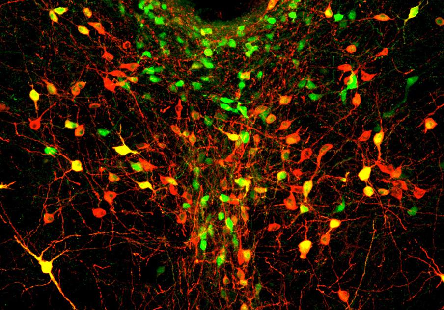
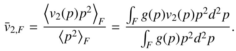
This image of the dorsal raphe nucleus labels dopamine neurons in green, red, and yellow. This region of the brain is critical in generating the increased sociability that typically occurs after a period of social isolation. Image credit Gillian Matthews, Ungless Lab, Imperial College London.
Approximate Scale: 450 micrometers
Chemistry Section
This is a transmission electron microscope image of a graphene lattice. Graphene is a periodic structure entirely composed of carbon atoms. At this scale, individual atoms can be observed at the corners of the hexagons. Image credit Ethan Minot, Department of Physics, Oregon State University (Original grayscale image colorized). Approximate Scale: 4 nanometers
Engineering Section
Visualizing patterns of air traffic over the contiguous United States reveals major airports and commonly flown-over regions. The darkest areas receive little-to-no flyovers. Image credit Aaron Koblin, Scott Hessels, and Gabriel Dunne, UCLA.
Approximate Scale: 4500 kilometers
Mathematics and Computer Science Section
The Opte Project aims to visualize the internet by mapping routing paths from all over the world. Each color represents computers from a different region of the world. This visualization is from 2015. Image credit Barrett Lyon/The Opte Project.
Approximate Scale: One zettabyte for the year 2015
Physics Section
The Baryon Oscillation Spectroscopic Survey (BOSS) Great Wall, a galaxy supercluster, is one of the largest structures in the observable universe. This image shows a simulation of how galaxy clusters form. The filaments are regions where galaxies are more likely to be found.
Image credit Volker Springel, Max Planck Institute for Astrophysics.
Approximate Scale: 1 billion light years
Back Cover
Scientific collaborations span the globe. This map depicts collaboration networks between researchers in different locations. Collaborations often - but not always - seem to follow linguisic and cultural connections. Image computed by Oliver H. Beauchesne and SCImago Lab, data by Elsevier Scopus.
Approximate Scale: 39,000 kilometers
44 Using a Hybrid Machine Learning Approach for Test Cost Optimization in Scan Chain Testing
LUKE DUAN, 2019
49 Novel Water Desalination Filter Utilizing Granular Activated Carbon
GEOFFREY FYLAK, 2019
Mathematics and Computer Science
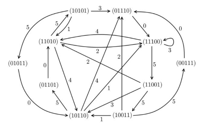
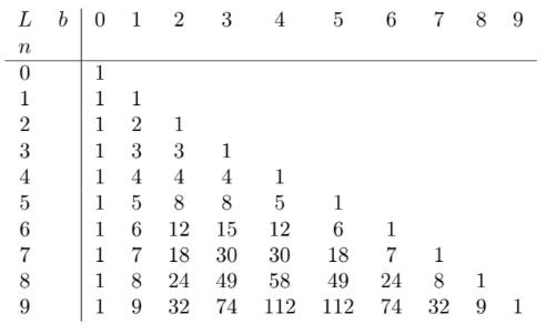
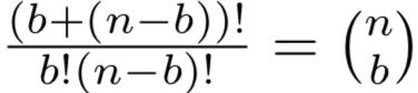
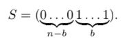
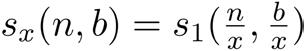
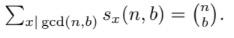
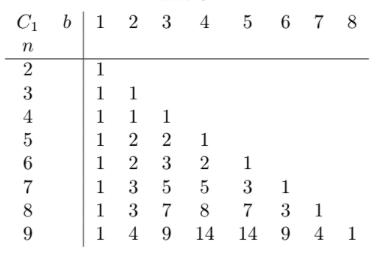
59 Long Prime Juggling Patterns
DANIEL CARTER AND ZACH HUNTER, 2019
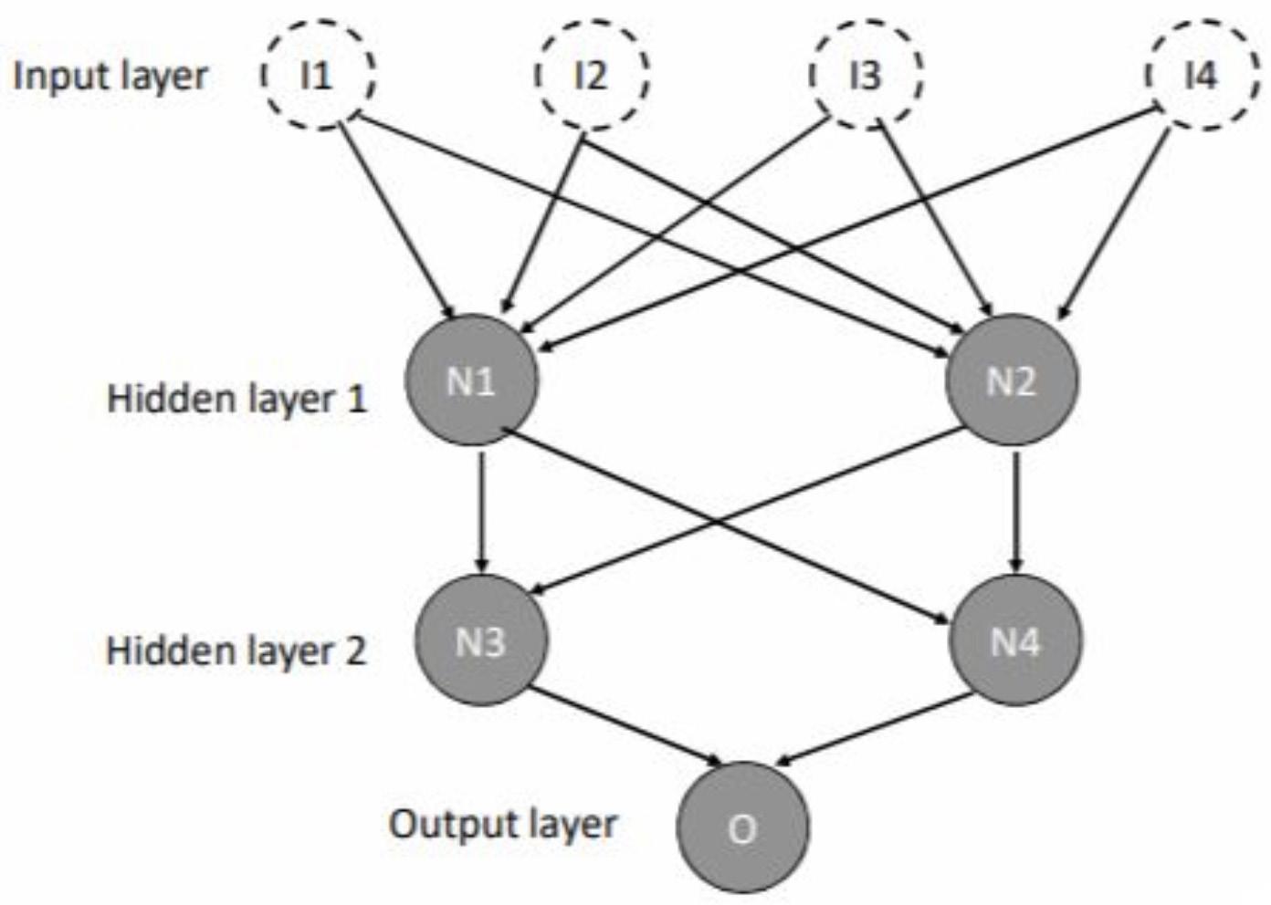
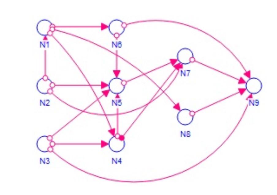
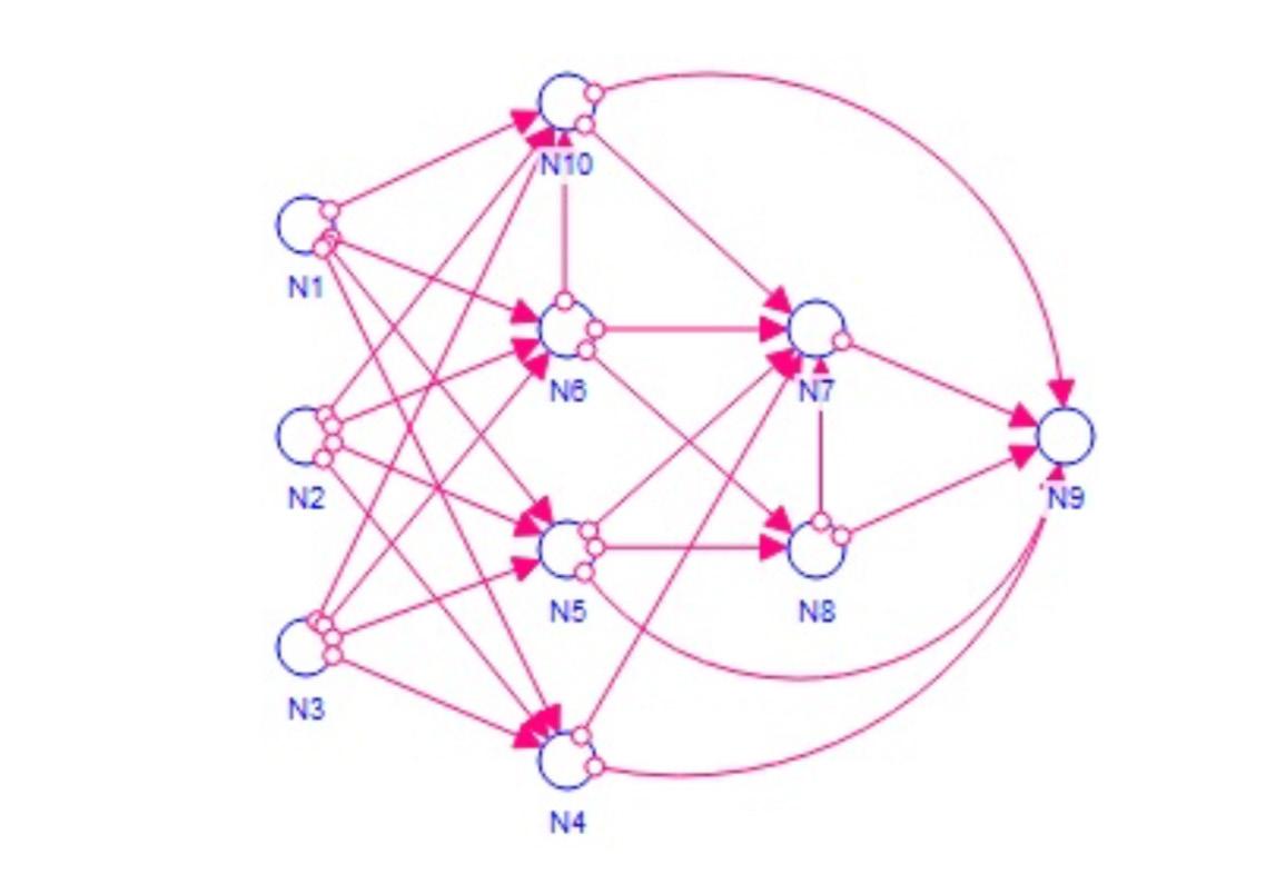
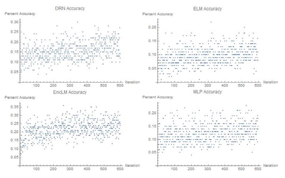
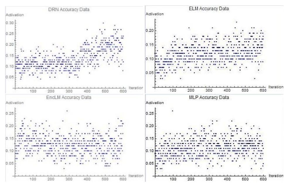
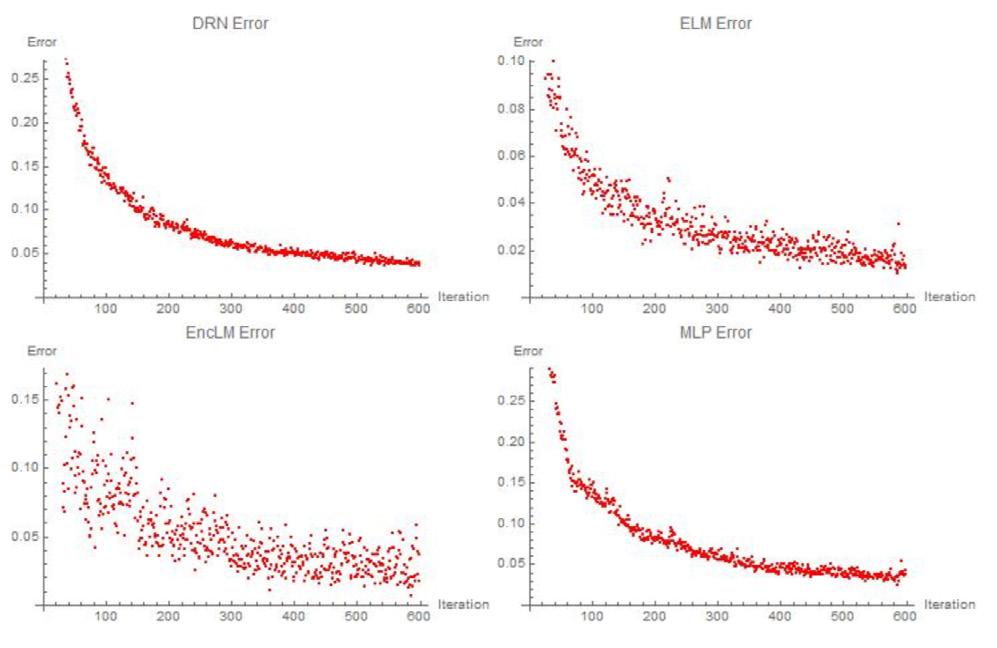
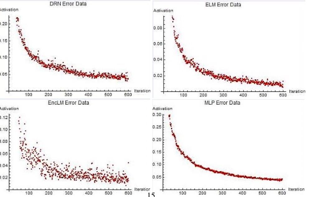
67 An Analysis of a Novel Neural Network Architecture
VATSAL VARMA, 2019 ONLINE
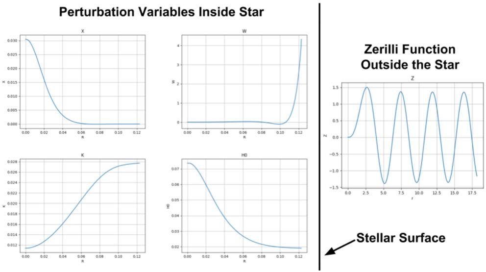
75 Effects of Relativity on Quadrupole Oscillations of Compact Stars
ABHIJIT GUPTA, 2019
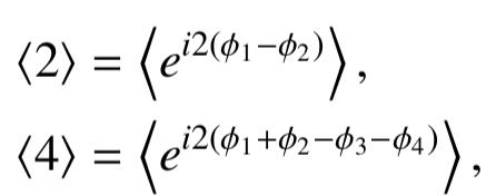
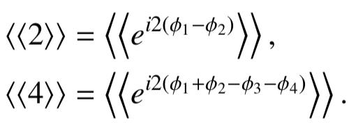
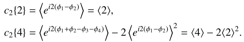
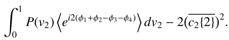
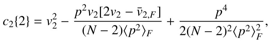
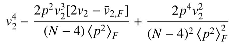
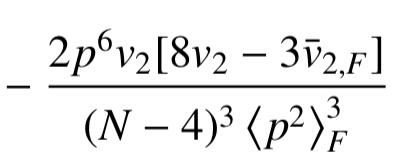
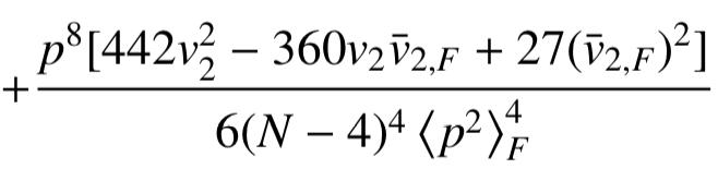
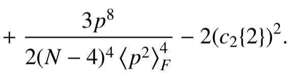
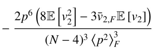
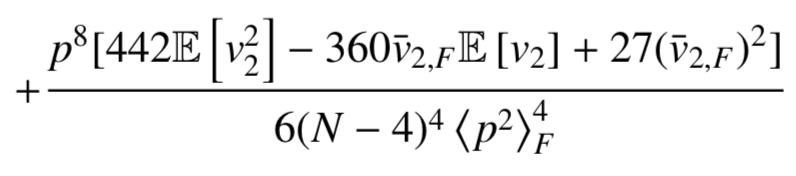
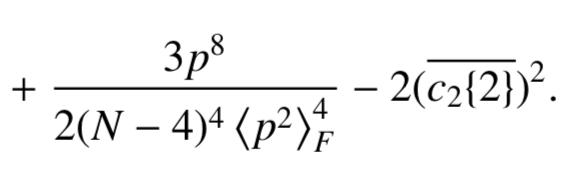
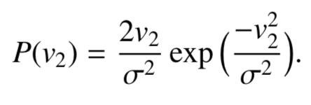
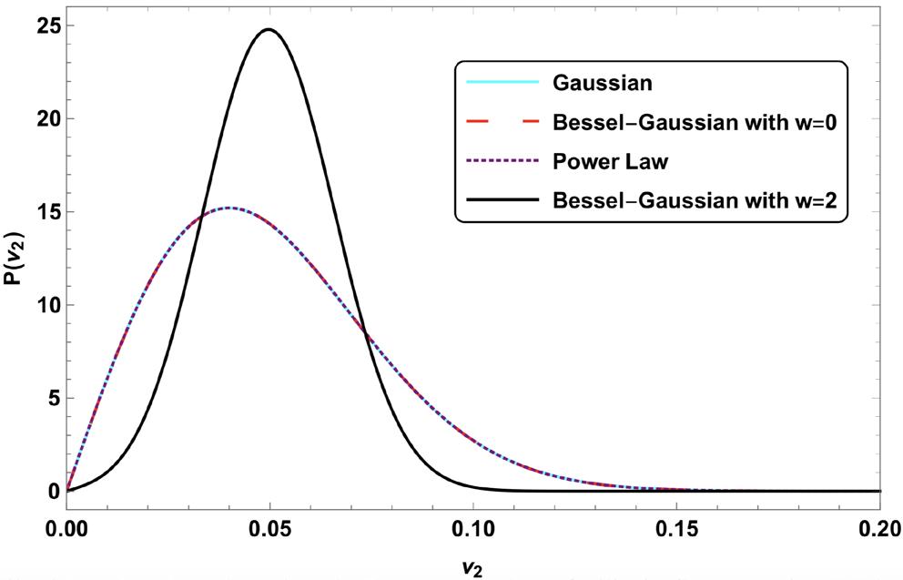
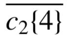
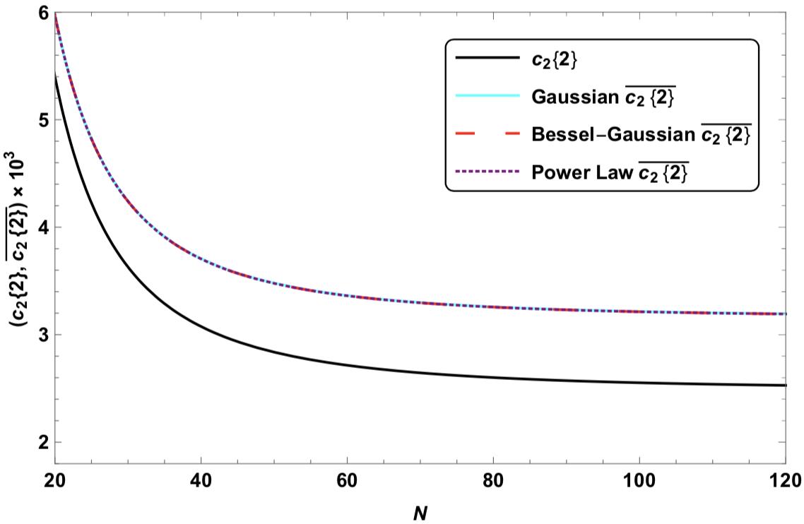
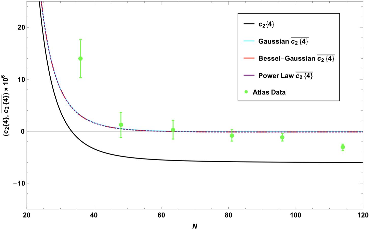
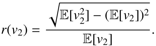
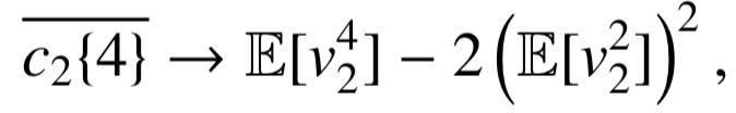
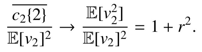
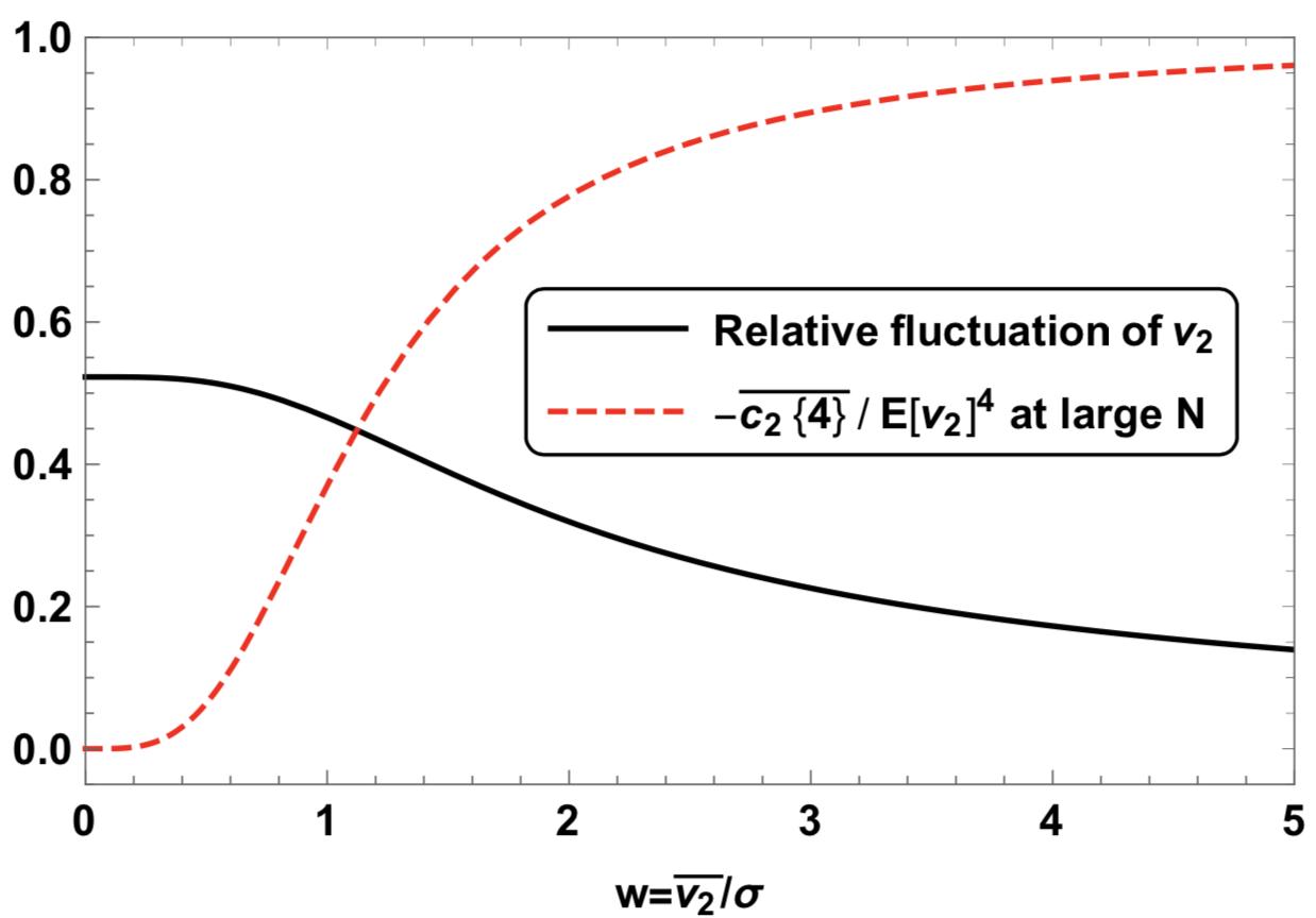
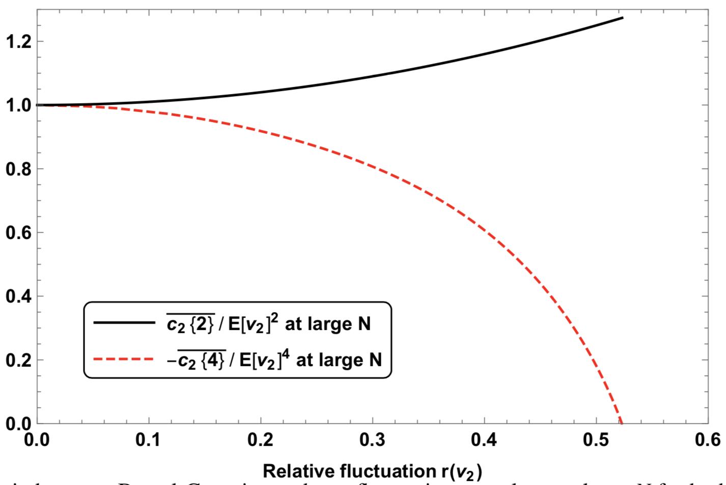
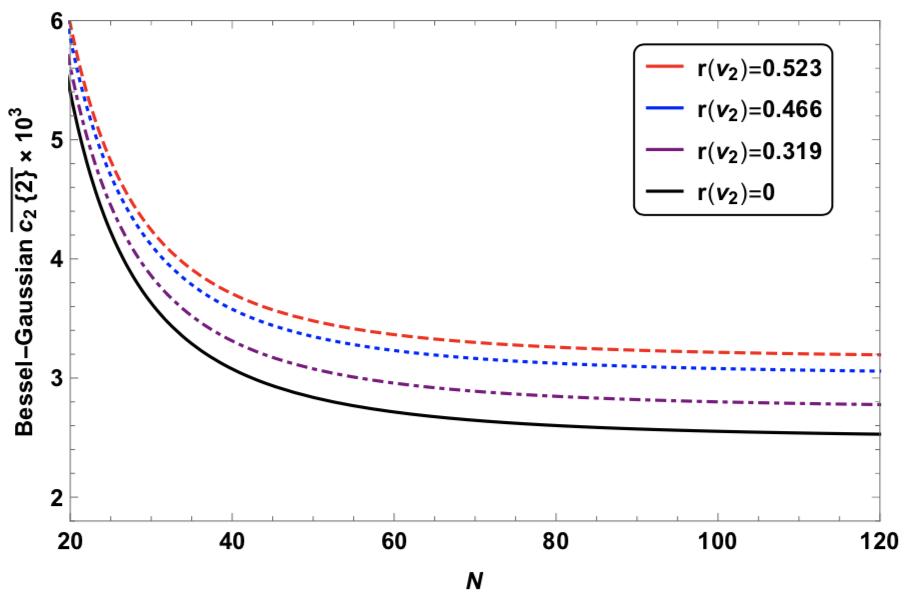
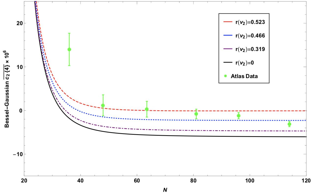
84 Effect of Elliptic Flow Fluctuations on the Two- and Four-Particle Azimuthal Cumulant
BRIAN LIN, 2019
Featured Article
89 An Interview with Dr. Valerie Ashby
LETTER from the CHANCELLOR
"Science is a cooperative enterprise, spanning the generations. It's the passing of a torch from teacher, to student, to teacher. A community of minds reaching back to antiquity and forward to the stars."
~ Dr. Neil deGrasse Tyson
I am proud to introduce the eighth edition of the North Carolina School of Science and Mathematics’ (NCSSM) scientific journal, Broad Street Scientific. Each year students at NCSSM conduct significant scientific research, and Broad Street Scientific is a student-led and student-produced showcase of some of the impressive research being done by students.
Excellence in scientific research has a deep and far-reaching impact on nearly every aspect of daily life, including (among other areas) health care, food safety, space travel, national security, and the environment. When NCSSM students are given opportunities to apply their learning through research, they are doing more than increasing their individual knowledge; their valuable work is increasing our collective body of knowledge and strengthening our ability to address current global challenges and prepare for those to come.
Opened in 1980, NCSSM was the nation’s first public residential high school where students study a specialized curriculum emphasizing science and mathematics. Teaching students to do research and providing them with opportunities to conduct high-level research in biology, chemistry, physics, computational science, engineering and computer science, math, humanities, and the social sciences are critical components of NCSSM’s mission
to educate academically talented students to become state, national, and global leaders in science, technology, engineering, and mathematics. I am thrilled that each year we continue to increase the outstanding opportunities NCSSM students have to participate in research.
This publication serves to highlight some of the high quality research students conduct each year at NCSSM under the direction of our outstanding faculty and in collaboration with researchers at major universities. For thirty-four years, NCSSM has showcased student research through our annual Research Symposium each spring and at major research competitions such as the Regeneron Science Talent Search and the International Science and Engineering Fair. The publication of Broad Street Scientific provides another opportunity to share with the broader community the outstanding research being conducted by NCSSM students each year.
I would like to thank all of the students and faculty involved in producing Broad Street Scientific, particularly faculty sponsor Dr. Jonathan Bennett, and senior editors Emily Wang, Navami Jain, and Kathleen Hablutzel. Explore and enjoy!
Dr. Todd Roberts, Chancellor
WORDS from the EDITORS
Welcome to the Broad Street Scientific, NCSSM’s journal of student research in science, technology, engineering and mathematics. In this eighth edition of Broad Street Scientific, we hope to inspire readers to get involved in the scientific community by sharing the innovative research conducted by our students. We hope you enjoy this year’s edition!
This year’s theme is networks: the connections we find within and between groups throughout our world. Connectivity is an integral component of modern life, and studying people or objects interacting in networks allows us to describe collective behavior of groups. Billions of interconnected neurons comprise the human brain, yet a brain is more than a bunch of cells. Brains can think, feel, and act both consciously and unconsciously. Thus, networks do not simply behave as the sum of their parts. Networks are powerful in predicting the complex behavior of a dynamic group without needing complex information on each individual in a network. For example, networks can predict the spread of an infectious disease without needing information on each individual in the network. Networks are powerful tools in describing our interconnected world.
In the featured images of this journal, we explore the scales of networks, from the atomic to astronomical levels. The featured image for the Chemistry section displays a network of carbon atoms on the scale of fractions of
a nanometer, while the featured image for the Physics section displays a network of superclusters of galaxies on the scale of approximately one billion light years – one of the largest known structures in the universe. On any scale, our world is built on interactions, and these interactions organize our world into networks.
We would like to thank the faculty, staff and administration of NCSSM for their continued support towards our student researchers. It is this unmatched encouragement that prepares us to use our interests and skills in STEM to address problems in our community, both locally and beyond. For 39 years, NCSSM has fostered an environment conducive to learning through encouraging students to take risks and take ownership of their academic path. We would especially like to thank our faculty advisor, Dr. Jonathan Bennett, for his support and guidance throughout the publication process. We would also like to thank Chancellor Dr. Todd Roberts, Dean of Science Dr. Amy Sheck, and Director of Mentorship and Research Dr. Sarah Shoemaker. Lastly, the Broad Street Scientific would like to acknowledge Dr. Valerie Ashby, chemistry professor and Dean of Trinity College of Arts and Sciences at Duke University, for speaking with us about her inspiring journey in STEM and offering advice to young prospective scientists.
Kathleen Hablutzel, Navami Jain, and Emily Wang Editors-in-Chief
BROAD STREET SCIENTIFIC STAFF
Editors-in-Chief
Kathleen Hablutzel, 2019
Navami Jain, 2019
Emily Wang, 2019
Publication Editors
Rohit Jagga, 2020
Grishma Patel, 2019
Sanjana Pothugunta, 2020
Eleanor Xiao, 2020
Biology Editors
Megan Wu, 2019
Ishaan Maitra, 2020
Joseph Wang, 2020
Chemistry Editors
Melody Wen, 2020
Varun Varanasi, 2020
Engineering Editors
Aakash Kothapally, 2020
Jason Li, 2020
Mathematics and Computer Science Editors
Physics Editors
Hahn Lheem, 2019
Olivia Fugikawa, 2020
Will Staples, 2020
Ben Wu, 2020
Faculty Advisor
Dr. Jonathan Bennett
THE AI WE HAVEN'T CONSIDERED
Jackson Meade
Jackson Meade was selected as the winner of the 2018-2019 Broad Street Scientific Essay Contest. His award included the opportunity to interview Dr. Valerie Ashby, distinguished chemist and professor and Dean of Trinity College of Arts and Sciences at Duke University. This interview can be found in the Featured Article section of the journal.
“People worry that computers will get too smart and take over the world, but the real problem is that they’re too stupid and they’ve already taken over the world.”
~ Pedro Domingos
When we bring up artificial intelligence in conversation, the rhetoric is relatively future-oriented. Discussions about the “possibilities” AI possesses – and the dangers it poses – abound, all in the context of what our technological future holds. But peel back the layer of speculation, and you may find something surprising. It might not be obvious, but artificial intelligence is already here – in fact, it’s everywhere.
Though that statement sounds concerning, there isn’t a conspiracy of shadowy Artificial Intelligences operating behind the backs of the public. We’ve simply grown accustomed to its cohabitation in our systems. Artificial Intelligence, through “Machine Learning,” started accelerating in 1957, when Frank Rosenblatt designed the first Neural Network, called a perceptron (Lewis & Denning), to model the structure of the human brain (Marr). By 1985, Professor Terry Sejnowski had created NetTalk, which could pronounce 20,000 English words with just a week of training (New York Times).
When you flip through a stuffed email inbox, machine learning keeps it from exploding by marking most of the spam and trashing it, arguably with impressive precision (Aski & Sourati). Go to your search engine and type your query, and the “suggested search” bar that appears at the bottom, as well as the results your query generates, are the product of a well-trained, personalized machine learning algorithm (Schachinger). When you purchase something on Amazon or scroll through your recommended videos page on YouTube, a machine learning system makes sure you see the kinds of things you might want to watch or buy, even if you couldn’t articulate it yourself. If you are looking at a screen, it is likely that machine learning had its hands (for lack of a more computerized term) in it.
Since the early days of computing, computers have required painstaking algorithms – increasing by orders of magnitude in complexity – to do anything from displaying text to managing Google’s 40,000 search queries per second (Alphabet, Inc). This creates a ceiling of capabilities for our systems that grows infinitely harder to raise. But
computer systems are, after all, human systems, and we should model them that way. This is exactly what machine learning algorithms do. Based on inferences from the data we give them, they teach themselves how to analyze and manipulate it, and the more data we give them, the better they get at doing their jobs (Faggella) (Lewis & Denning). This is significantly “human” – barring willful ignorance, we get better at analyzing and understanding our world given new information.
Despite possible concerns, you are kept safe because of machine learning. In 2014, Kaspersky Lab's Anti-Malware Research Team processed between 200,000 and 315,000 malicious files per day (Kaspersky Lab). But malicious files aren’t so different from each other, so machine learning algorithms can very easily identify the code for files with malicious intent far faster than any human actors could. In a country and world growing ever more concerned with data security, these algorithms provide a necessary wall between us and the actions of evil people.
In our finances, we’re relinquishing control to the machines as well. Micromanagement of our funds is a multibillion-dollar business, and artificial intelligence completely disrupts it. While humans are good at predicting what the stock market can do over large spans of time because of noticeable trends, on smaller and smaller time scales and in more volatile markets, our grand spending schemes are fundamentally nothing short of guesswork. And while machine learning algorithms are admittedly built on guesswork, they can achieve super-human levels of accuracy during training on multitudes of data that are simply unattainable for even the most dedicated human.
Predicting stocks is not the only artificial-intelligenceguided moneymaker around. Advertising is one of the most lucrative businesses of the modern world, having generated about $32.66 billion dollars in revenue for Google’s parent company, Alphabet, in Quarter 2 of 2018 (D’Onfro). This comes from thousands of paying customers, all of them companies hoping their product appeals to the right niche, and only works because of machine learning.
In this realm, one cannot avoid the topic of driverless cars. Artificial intelligences are crucial to computer vision algorithms (Khirodkar, Yoo, & Kitani), though other hard-coded solutions can aid them. 74% of automotive company executives expect that these smart cars will be on the road by 2025, according to a report from IBM (IBM). The menial tasks of our lives – our driving, our purchases – will be automated if they can be.
We have been exploring the risks of developing artificial intelligences prior to the day we could make them. In 1942, science fiction author Isaac Asimov published his nowfamous laws of robotics in a short story, “Runaround.” They stated:
First, “A robot may not injure a human being or, through inaction, allow a human being to come to harm.”
Second, “A robot must obey the orders given to it by human beings, except where such orders would conflict with the First Law.
Third, “A robot must protect its own existence as long as such protection does not conflict with the First or Second Law.”
But restricting our concerns about Artificial Intelligence to this view is too narrow. It comes from an assumption about the types of intelligences we intend to create. It assumes that we will “build ourselves” – that we will build copies of humans, in humanoid robot bodies with human emotions and human capabilities.
We are a species that changes its environment to fit its needs instead of adapting to its surroundings. Machine learning and artificial intelligence are the newest evolution of this pattern – just another way that the world and the patterns within it can be adjusted according to our wishes. The patterns of our world once influenced us to a degree we could not control, but artificial intelligence will allow us to take full control and then completely relinquish it. All this works because machine learning is based in prediction – on understanding the once-unintelligible patterns that comprise the fabric of our world. That is a flaw that could spell the end of our humanity.
It seems unlikely a malicious AI will attempt to literally end life on Earth. At the least, we have Asimov’s three laws to thank for that. But in a world where everything can be predicted, where everything we want to see can be shown to us, and where things that are “unpopular” or “troubling” never reach our eyes, it feels like a part of our humanity is lost. An artificial intelligence could operate in plain sight, tailoring our world to the patterns that dictate us. As mentioned, artificial intelligences are human systems, so they will follow the human model of changing the world to fit their needs. It is reasonable that if our needs rely on a series of predictable patterns, then an artificial intelligence with benevolent intentions could inadvertently neutralize the world’s ideological diversity and the differences that give us the human condition.
This isn’t to say that we shouldn’t create artificial intelligences – in fact, it seems clear that our modern world couldn’t operate without them. There are proactive steps we must take to be stewards of our humanity. We must make an active choice to diversify our interests and the viewpoints to which we expose ourselves, even when they aren’t completely satisfying. We should model another fundamental element of our humanity into our artificial intelligences: variation. Our machine learning algorithms cannot rely on optimizing patterns alone – they must contain anomalies in their paradoxically predictive, average-based algorithms. If we do this, we can ensure that our artificial intelligences will enhance us instead of dictating conformity.
References
A Q & A with Pedro Domingos: Author of ‘The Master Algorithm’ [Interview by J. Langston]. (2015, September 17). Retrieved January 4, 2019, from https://www. washington.edu/news/2015/09/17/a-q-a-with-pedrodomingos-author-of-the-master-algorithm/
Aski, A. S., & Sourati, N. K. (2016). Proposed efficient algorithm to filter spam using machine learning techniques. Pacific Science Review A: Natural Science and Engineering, 18(2), 145-149. doi:10.1016/j. psra.2016.09.017
D’Onfro, J. (2018, July 23). Alphabet jumps after big earnings beat. Retrieved January 7, 2019, from https:// www.cnbc.com/2018/07/23/alphabet-earnings-q2-2018. html
Faggella, D. (2018, December 21). What is Machine Learning? | Emerj - Artificial Intelligence Research and Insight. Retrieved January 9, 2019, from https://emerj. com/ai-glossary-terms/what-is-machine-learning/
Google Search Trends, Search Per Second. (n.d.). Retrieved January 12, 2019, from https://trends.google. com/trends/?geo=US
IBM (2015). Automotive 2025: Industry without Borders. IBM Institute for Business Value. Retrieved January 9, 2019, from http://www-935.ibm.com/services/ multimedia/GBE03640USEN.pdf
Kaspersky Lab is Detecting 325,000 New Malicious Files Every Day. (n.d.). Retrieved January 5, 2019, from https://www.kaspersky.com/about/press-releases/2014_ kaspersky-lab-is-detecting-325000-new-malicious-filesevery-day
Khirodkar, R., Yoo, D., & Kitani, K. M. (2018). VADRA: Visual Adversarial Domain Randomization and Augmentation. Carnegie Mellon University. Retrieved December 10, 2018, from https://arxiv.org/ pdf/1812.00491.pdf
Learning, Then Talking. (1988, August 16). Retrieved January 6, 2019, from https://www.nytimes. com/1988/08/16/science/learning-then-talking.html
Lewis, T. G., & Denning, P. J. (2018). The Profession of IT: Learning Machine Learning. Communications of the ACM, 61(12), 24-27. Retrieved December 26, 2018, from https://calhoun.nps.edu/bitstream/handle/10945/60898/ Denning_Learning_Machine_Learning_ACM_2018-12. pdf?sequence=1&isAllowed=y.
Levenson, E. (2014, January 31). The TSA is in the Business of ‘Security Theater,’ Not Security. Retrieved January 7, 2019, from https://www.theatlantic.com/ national/archive/2014/01/tsa-business-security-theaternot-security/357599/
Marr, B. (2016, March 08). A Short History of Machine Learning -- Every Manager Should Read. Retrieved January 5, 2019, from https://www.forbes.com/sites/ bernardmarr/2016/02/19/a-short-history-of-machinelearning-every-manager-should-read/#2493077c15e7
Matney, L. (2017, May 17). Google has 2 billion users on Android, 500M on Google Photos. Retrieved January 5, 2019, from https://techcrunch.com/2017/05/17/googlehas-2-billion-users-on-android-500m-on-google-photos/
Schachinger, K. (2018, December 06). A Complete Guide to the Google RankBrain Algorithm. Retrieved January 4, 2019, from https://www.searchenginejournal.com/ google-algorithm-history/rankbrain/
Scott, T. (2018, December 06). Retrieved January 13, 2019, from https://www.youtube.com/watch?v=JlxuQ7tPgQ
Wu, J., Zhang, C., Xue, T., Freeman, W. T., & Tenenbaum, J. B. (2016). Learning a Probabilistic Latent Space of Object Shapes via 3D Generative-Adversarial Modeling. Advances In Neural Information Processing Systems, 29. Retrieved November 11, 2018, from https:// arxiv.org/abs/1610.07584.
Yoganarasimhan, H. (2017). Search Personalization Using Machine Learning. SSRN Electronic Journal. doi:10.2139/ssrn.2590020
OVEREXPRESSION OF A HEAT SHOCK PROTEIN IN CYANOBACTERIA TO INCREASE GROWTH RATE
Robert Landry
Abstract
To increase earth’s capacity to support human population growth, methods of growing food more efficiently, especially in warmer environments as climate change progresses, must be developed. This project sought to increase the growth rate of one population of photosynthetic organisms, cyanobacteria, through genetic engineering. Synechococcus elongatus UTEX 2973 cultures were transformed to overexpress dnaJ, a heat shock protein, in normal and heat-stressed conditions to determine the gene’s effects on growth rates. The growth rates of the dnaJ overexpressing strain were related to the control--wild-type Synechococcus elongatus UTEX 2973 transformed with a plasmid without dnaJ--through comparisons of optical density measurements at 745 nanometers (OD745), which can accurately quantify growth rates. The change in OD745 in the dnaJ overexpressing strain was significantly greater than the OD745 measurements for the control in normal conditions. When the temperature was increased to 42˚C, the dnaJ overexpressing strain continued to grow, while the control strain’s OD745 measurements decreased. From this data, it appeared that the overexpression of a heat shock protein in the genome of cyanobacteria significantly increased their growth rates and provided heat resistance. Researching the effects of overexpressing a heat shock protein could be furthered in organisms such as corn, rice, soybeans, and other photosynthetic species.
1. Introduction
Cyanobacteria, bacteria that conduct photosynthesis, have the potential to revolutionize both agricultural practices and the food industry, if higher yields of target materials are attained (Chow et al., 2015). Cyanobacteria, capable of utilizing 10% of the sun’s energy, are nearly 10 times more efficient at fixing carbon found in CO2 than other energy plants such as sugar cane or corn, which harness only 1% of the sun’s energy (Hunt, 2003). This efficiency drives cyanobacteria into the energy industry’s spotlight as a possible, influential source of energy for humanity. Moreover, their increased photosynthetic rates decrease the amount of CO2 in the atmosphere, which benefits the global environment. Five other aspects of these photosynthetic bacteria that interest scientists are that they: grow in high densities, use water as an electron donor, utilize infertile land, require non-food-based feedstock, and thrive in many different water conditions (brackish, fresh, or saltwater) (Parmar et al., 2015).
Although all of these benefits already apply to cyanobacteria, it is still expensive to culture, grow, and eventually utilize the products of the bacteria in an efficient way. In order for cyanobacteria to be widely used, a sharp increase in target yields and decrease in expense must occur in order to compete with the simplicity and economic benefits of plants.
Coupled with being more cost-effective when producing target materials, plants have also been genetically modified with genes originating from cyanobacteria to increase efficiency. For example, carbon fixation rates in transgenic tobacco were increased significantly after transforming
cyanobacterial Rubisco into the tobacco’s genome. Photosynthetic efficiency was increased as a result of cyanobacteria’s efficiency, which serves as a precedent for future research (Occhialini et al., 2015).
This transgenic tobacco demonstrates the viability of increasing the efficiency of plant growth with cyanobacteria research. This pursuit is important because scientists of the Global Harvest Institute estimate that the world could face a food crisis by 2030 (Martin, 2017). Developing new methods of growing crops is paramount to mitigating this impending humanitarian need.
In recent decades, knowledge regarding cyanobacteria has increased exponentially, stemming first from the genome-mapping of Synechocystis sp. 6803, one species of cyanobacteria. Now there are more than 128 different strains of cyanobacteria fully sequenced, which provides many opportunities in genetic engineering to study the properties of the bacteria. This developing field of genetic engineering allows researchers to utilize various transformation techniques in order to optimize photosynthetic rates within cyanobacteria, and ultimately in other organisms as well (Al-Haj et al., 2016).
The species Synechococcus elongatus PCC7942 is one species of cyanobacteria that has had its entire genome sequenced and therefore is a candidate for many genetic engineering projects that study photosynthetic processes, regulation of nitrogen-containing compounds, and acclimation to stressed conditions (Home - Synechococcus elongatus PCC 7942). Synechococcus elongatus PCC7942, previously known as Anacystis nidulans R2, is a freshwater cyanobacteria that was the first cyanobacteria to be successfully transformed using exogenous DNA (Shestakov
Table 1. The list of forward and reverse primers used for isolating dnaJ.
Synechococcus elongatus
UTEX L 2973
Synechococcus elongatus
UTEX L 2973
Synechococcus elongatus
UTEX L 2973
Synechococcus elongatus
dnaJ Forward 69.2
dnaJ Reverse 68.19
dnaJ Forward 68.16
UTEX L 2973 dnaJ Reverse 67.47
& Khyen, 1970). Synechococcus elongatus PCC7942 are obligate photoautotrophs, which means that they only rely on their photosynthetic ability to produce nutrients instead of being able to break down and use nutrients found in their environment (Minda et al., 2008). Due to this attribute, Synechococcus elongatus PCC7942’s photosynthetic efficiency must be optimized for any condition, including stress, to outlast their natural competition. One such way that Synechococcus elongatus PCC7942 has been shown to adapt to extreme heat and high light conditions is the induction of the dnaK and dnaJ genes (Hihara et al., 2001).
The gene dnaK has three different homologues found in the genome of Synechococcus elongatus PCC7942, designated dnaK1, dnaK2, and dnaK3. DnaK1’s function is unknown in the Synechococcus elongatus PCC7942, although it is known to be found in the cytosol of the cyanobacteria. Both dnaK2 and dnaK3 are essential for the growth of Synechococcus elongatus PCC7942 (Watanabe, 2007). Similar to dnaK, dnaJ has 4 homologues within the Synechococcus elongatus PCC7942 genome, referred to as dnaJ1, dnaJ2, dnaJ3, and dnaJ4. DnaJ3 has been found to be located in the membrane of the cyanobacteria. DnaJ2 is shown to be induced in extreme heat and high light conditions. Apart from these two homologues, dnaJ2 and dnaJ3, most of dnaJ roles in the cell have not been discovered (Shestakov & Khyen, 1970). The substitute for Synechococcus elongatus PCC7492 that will be used in this experiment due to budget constraints is Synechococcus elongatus UTEX L 2973. Within Synechococcus elongatus UTEX L 2973, there are 10 homologues of dnaJ (Genome). Their respective roles within the cell beyond molecular chaperones are largely unknown, apart from dnaJ3, which is a known heat shock protein (Genome). The third homologue of dnaJ was isolated and overexpressed in a transformed strain of cyanobacteria in this research project.
The goal of this project is to determine the effects of dnaJ on the photosynthetic rate of Synechococcus elongatus UTEX L 2973 and explore the correlation between the
Sequence (5’-3’) Purpose
GAGAATTCATGGGTCGTCGCTGGA Transformation
GAGGATCCCTAGCATGCAAGCTCTCCTG Transformation
ATGCAAAATTTTCGCGACTACTATGCC RT-PCR
TCAACGCGATTGTTCGAGCGAT RT-PCR
genes’ overexpression and growth rates in various heat conditions. This research could lead to new advancements in industry and agriculture through the higher production rates of glucose and target materials.
2. Methods
2.1 – Culturing Synechococcus elongatus UTEX L 2973
Synechococcus elongatus UTEX L 2973 thrive in BG-11 liquid medium at 30°C under 12-hour light cycles from a Percival Incubator. Once the cyanobacteria showed initial growth in the medium, the bacteria were aliquoted to more containers to protect the Synechococcus elongatus UTEX L 2973 from contamination that could ruin the whole strain (Kufryk et al., 2002).
2.2 – DNA extraction, PCR and RT-PCR
The DNA from Synechococcus elongatus UTEX L 2973 was extracted using the QIAamp DNA Mini Kit and its corresponding protocol (QIAGEN). Using the primers listed in Table 1, dnaJ was isolated including the restriction enzyme cut sites necessary for ligation. The PCR was run according to the OneTaq Hot Start protocol (Biolabs). The extension phase lasted for 2 minutes and the annealing temperature was 61°C.
2.3 – Cloning
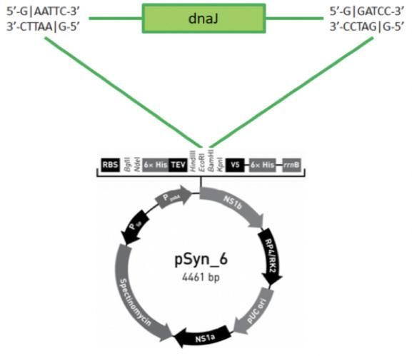
Using BamHI and EcoRI restriction enzymes, dnaJ was ligated into the plasmid pSyn_6 from a GeneArt Synechococcus Engineering Kit.
2.4 – Transformation of E. Coli
A 5-alpha E. coli strain was transformed using the heat shock method to replicate the desired plasmid. Two different plasmids were used to transform the E. coli, one vector without dnaJ and one plasmid including dnaJ. After transformation, the E. coli grew in SOC medium, which was then spread on LB plates with spectinomycin at 50
μg/mL concentration. After growing overnight, colonies were labeled and were inoculated into tubes corresponding to their label to grow overnight.
2.5 – Transformation of Synechococcus Elongatus UTEX L 2973
The plasmid DNA from the E. Coli was extracted using a Spin Miniprep Kit and its corresponding protocol. This plasmid DNA was then used to transform Synechococcus Elongatus UTEX L 2973 following the protocol provided by GeneArt Synechococcus Engineering Kit. This vector has not been used to transform pSyn_6 before.
2.6 – Statistical Analysis
To analyze the OD745 data, error bars were calculated by multiplying the standard error of the mean by two. To test significance, a t-test calculator for the comparison of means was used to determine a p-value. One asterisk (*) represents significance at a p-value of < .05; two asterisks (**) concludes significance at a p-value of < .01; three asterisks (***) demonstrates that the data are significant at a p-value of < .005
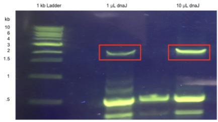
show the successful isolation of dnaJ, a gene of length 1.8kb (Fig. 2a).
2a. Successful PCR amplification of dnaJ. The band at 1.8kb is dnaJ.
2b. The cutout portion of the gel isolated the vector that was used in gel extraction and ligation.
2c. Cutouts from the gel isolated dnaJ. These bands were ligated into the plasmid after gel extraction.
3.1 – Cloning Strategy
A cloning strategy was used (Fig. 1). DnaJ was isolated including the restriction enzyme cut sites necessary for ligation using the aforementioned primers (Table 1). The enzymes cut the target gene at the lines on either side of dnaJ (Fig. 1). The vector for GeneArt also had the same two restriction enzyme cut sites, BamHI and EcoRI, as the isolated gene. Utilizing DNA Ligase, the dnaJ was inserted into the plasmid in the 5’-3’ direction with a constitutively active promoter, PpsaA (NEB).
The bands around 1.8kb surrounded by the red boxes
Figure 2d. Gel electrophoresis of restriction enzyme digested plasmid from transformed E. coli. The bands at 1.8kb and 4.5 kb in lane 7 demonstrate correct ligation and transformation of the E. coli colony. Plasmid from this colony was used to transform Synechococcus elongatus UTEX L 2973.
Figure 1. dnaJ will be inserted in between EcoRI and BAMHI
3. Results
Figure
Figure
Figure
Following the preliminary PCR, another PCR reaction was run, and its products were cut with restriction enzymes before being exposed to ultraviolet light. Ultraviolet is a known DNA mutagen and hence, exposing dnaJ to this light before transformation in the cyanobacteria could alter its natural use in the cell. The vector was also cut with the restriction enzymes, BamHI and EcoRI. These two cut products were run through gels to purify the digested DNA (Fig 2b & 2c). Once the products were cut out, gel extraction was run to purify the DNA from the gel, so that ligation could be run (QIAquick). After the ligated plasmid was formed using DNA Ligase and a ligation buffer, the E. coli strain 5-alpha from New England Biolabs was transformed using heat-shock method (Fig. 1). 1, 3, and 6 μL of extracted DNA solution were added into separate vials of transformation-competent E. coli cells and were mixed gently. This mixture was put on ice for 30 minutes then heat-shocked at 42°C for 30 seconds without shaking. The transformed E. coli was put on ice for 2 minutes. 250 μL of room temperature SOC medium was added to the vial of E. coli. This vial was incubated shaking horizontally at 55 rpms at 37°C for 1 hour. Following the incubation, the various tubes of transformed E. coli were plated on separate solid LB medium plates with spectinomycin at a concentration of 50 μg/mL. The plates were incubated overnight at 37°C. Because of the presence of spectinomycin on the plates and the plasmid’s resistance to spectinomycin, the colonies that grew on the plate overnight had to contain the target plasmid.
Once the colonies formed, 12 colonies were isolated and grown individually in 3.0 mL of LB medium with spectinomycin at a concentration of 50 μg/mL overnight. The plasmid was isolated from these vials of transformed E. coli using the Spin Miniprep Kit (QIAprep). The plasmid was digested by EcoRI and BamHI. Gel electrophoresis was conducted to determine whether or not the plasmid incorporated the target gene properly (Fig. 2d). Culture 6 replicated the desired plasmid as seen by the bands at 4.5kb and 1.8kb, so the remaining plasmid that was not run through the gel was used to transform Synechococcus elongatus UTEX L 2973.
3a. Two colonies transformed with only vector in the presence of 10 μg/mL spectinomycin.
3b. Six colonies overexpressing dnaJ in the selective presence of spectinomycin.
3.2 – Transformation
The cyanobacteria were transformed using the protocol corresponding to the GeneArt Synechococcus Engineering Kit. Following transformation, the cyanobacteria were plated on solid BG-11 media with 10 μg/mL spectinomycin under normal conditions. Colonies formed and overexpressed dnaJ, and those that were transformed with only pSyn_6 plasmid grew (Fig. 3a & 3b). All of these colonies were numbered and then inoculated into flasks containing liquid BG-11 media with 10 µg/mL spectinomycin.
Figure
Figure
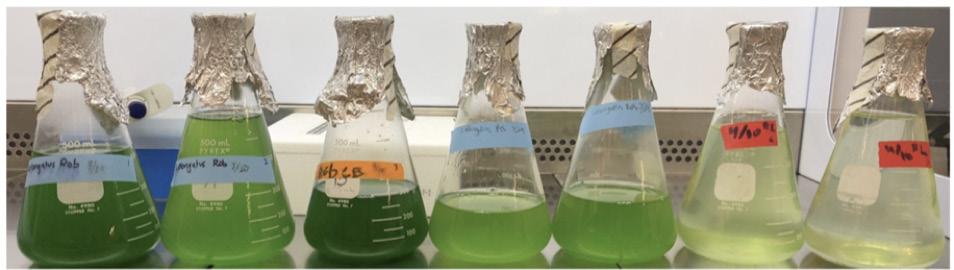
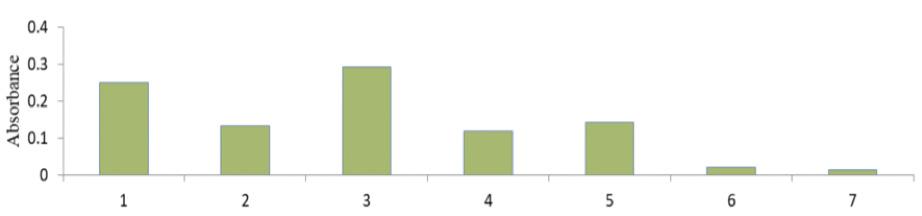
Figure 4a. Flasks with varying optical densities. The three flasks on the left were cultured for the longest time and thus, had the highest optical densities. The flasks on the right had grown more recently and were not as dark.
Figure 4b. Optical density values of corollary flasks. Higher optical densities correspond to darker flasks.
In order to determine the effects of dnaJ’s overexpression on growth rates within cyanobacteria, optical density measurements were taken from different cultures at 745 nanometers (nm) at varying temperatures. This is an appropriate wavelength because optical density measures turbidity instead of absorbance. The absorbance of the selected wavelength should be negligible in order for the measurements to strictly account for the reflection of light off of the cells in the solution (Martin, 2014).
There were 7 flasks of cyanobacteria before transformation with varying optical densities (Fig. 4a). In order to demonstrate what color and darkness of flasks correlates to OD745 values, optical density measurements corresponding to cyanobacteria culture were graphed (Fig. 4b). From the left to right, the optical density values were: .250, .133, .292, .119, .144, .022, .014. The darkest flasks evidently have the highest optical density measurements. This growth assay measures the total increase in optical density over time. The higher the change in optical density is, the higher the rate of growth for the colony is. Thus, when testing the two different transformed strains of Synechococcus elongatus UTEX L 2973, the transformed strain overexpressing dnaJ should have the higher change in optical density if the heat shock protein overexpressed through dnaJ truly increases photosynthetic and growth rates.
Because dnaJ codes for a heat shock protein, it was suspected that the growth rates of the strain overexpressing this gene would be significantly greater in only heat stressed conditions in comparison to the cyanobacteria only transformed with the vector. It was believed that the growth rate in normal conditions would not be affected greatly by the heat shock protein because the overexpression would not be necessary to withstand high temperatures. However, once the growth rates were
tested, it appeared as if the overexpression resulted in increased rates in both conditions (Fig. 5a & 5b).
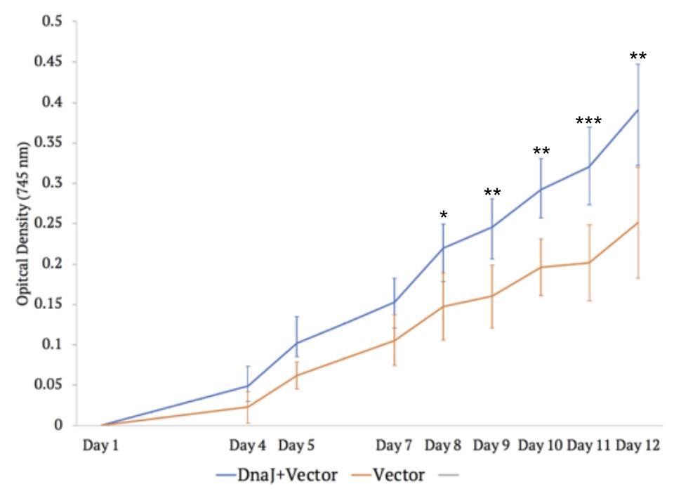
Figure 5a. Graph of optical density (745nm) of control stain and dnaJ overexpressing strain 30° Celsius. The data suggest dnaJ significantly increases growth rates.
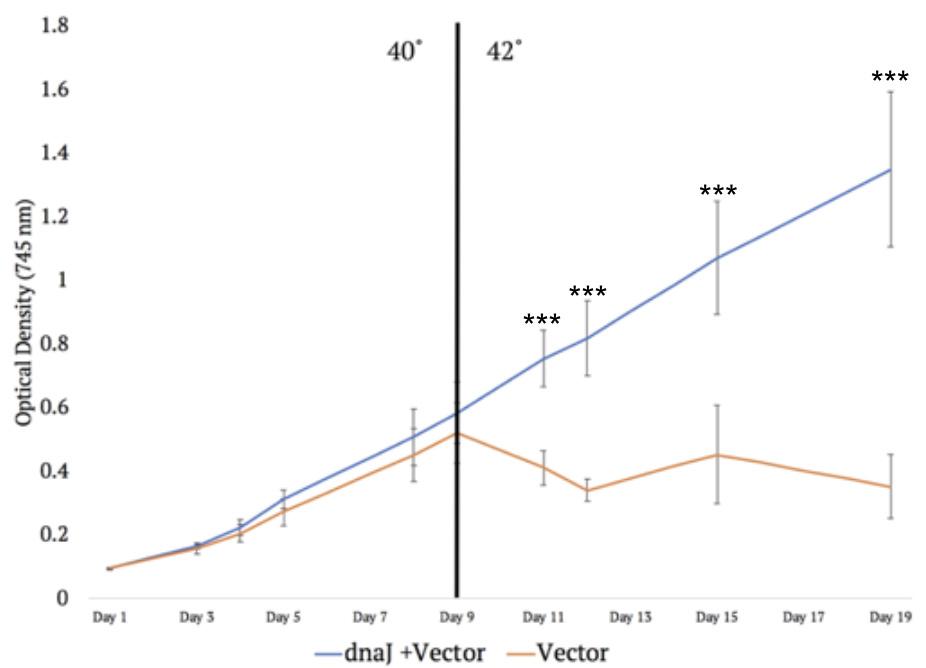
Figure 5b. The colonies were grown at 40° for 9 days. There was a trend in the data that indicates dnaJ promotes faster growth, but after the colony was exposed to a higher temperature, 42°, the control stain did not grow whereas the dnaJ strain continued normal growth. Data became significant two days after increased temperature.
The overexpression of dnaJ in normal conditions of 30°C and 12-hour light cycles increased the growth rate of the cyanobacteria significantly in comparison to the control. This significance was seen as early as day 8. The average OD745 of the dnaJ strain after 12 days was .39 in comparison to the vector strain that had an average OD745 of .25. This increase in optical density is attributed to the overexpression of dnaJ.
DnaJ’s overexpression within cyanobacteria in heat stressed conditions of 40°C and 12-hour light cycles also tended to increase growth rates. After 9 days, the average
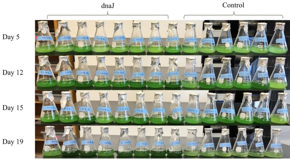
OD745 of the overexpressing strain was .58 while the other strain had an average of only .52; however, the standard deviation within each of the sample groups was too high to conclude significance at 40°. When the temperature in the Percival Incubator was increased to 42°, the dnaJ overexpressing strain grew normally, whereas the control strain’s average optical density decreased. The average optical density of the dnaJ overexpressing strain after 19 days was 1.35, and the control strain had an average optical density of .35. After just two days being exposed to the higher temperature, the difference between the two strains was significant, suggesting that the overexpression of dnaJ provided heat resistance to the transformed strain of cyanobacteria. There is a visual difference in optical density at day 19 in comparison to day 5, which demonstrates dnaJ’s potential to increase growth rates and provide heat resistance (Fig. 6).
Figure 6. The photo of the flasks in the top panel was taken on day 5. The flasks have similar tints of green. The last photo was taken on day 19. In the eight flasks on the left, the dnaJ overexpressing cultures have a much darker color than the control flasks.
4. Discussion
Essentially, this research sought to create a unique strain of cyanobacteria through genetic transformation. The specific plasmid utilized in the experimentation had not been used to transform Synechococcus elongatus UTEX L 2973 previously. The successful transformation as seen from the colony growth in the selective presence of spectinomycin demonstrates the competence of the plasmid pSyn_6 in transforming the experiment’s specific strain.
Despite the successful outcome of the research, there were several limitations in the experiment due to equipment and budget restrictions. One such limitation was the inability to determine the difference between the rates of oxygen evolution in the two strains. This would have led to a more precise measurement of the photosynthetic rate because oxygen is directly produced in photosynthesis. Optical density is a less direct measurement of this rate, but accurate, nonetheless. Without the generation of sugars through photosynthesis, the strains
could not grow. Because of this, higher photosynthetic rates should correspond to higher growth rates. Another limitation of this experiment was the inability to confirm gene expression in the transformed strains. However, confirming the correct plasmid makes it reasonable to assume that the growth rates increased on account of dnaJ overexpression.
This beneficial genetic overexpression has many potential applications in both the agriculture and energy industries. Because cyanobacteria are currently the most photosynthetically efficient organisms on the planet, this modification could lead to future applications in agriculture or more economic biofuel production that will capitalize on their efficiency (Hunt, 2003). One possible application could be the production and secretion of sugars for consumption. Because cyanobacteria are not seasonal like sugar cane, they could produce sugars more consistently and more efficiently, especially following genetic engineering. Clearly, isolation of sugar from a cyanobacteria solution would have to be much cheaper for this to be a viable contender with sugar cane, but nonetheless, this could be a potential application of genetically engineered cyanobacteria. Beyond sugars, cyanobacteria’s products have been manipulated to produce ethanol (Chow et al., 2015). Producing ethanol could prove to be a disruptive application of cyanobacteria in the energy industry, especially when paired with dnaJ overexpression.
Another possible application could be overexpressing heat shock proteins in other photosynthetic organisms to determine their effect on growth and photosynthetic rates. Overexpressing either dnaJ or corollary proteins specific to certain species within corn, rice, or soybeans could lead to increased production of these crops both in fertile geographies and in regions that are currently considered arid. Because heat shock proteins increased growth in Synechococcus elongatus UTEX L 2973 even in heat stressed conditions, it could be possible to genetically engineer cash crops to make them resistant to higher temperatures. This resistance could lead to the cultivation of previously infertile land, feeding millions more people worldwide. Further experimentation must be done to conclude the viability of any of these applications.
5. Acknowledgements
I would like to thank Dr. Monahan for teaching me the research process and guiding me through the fickle experimentation that is molecular biology. Thanks to her instruction and her patience with my stubborn commitment to this project, I was able to persevere through obstacles and accomplish my dream of genetically engineering cyanobacteria. I would like to thank Dr. Sheck for supervising me while I spent hours in the sterile
hood working with my cyanobacteria. I would also like to thank the rest of my Research in Biology colleagues for encouraging me throughout my time researching. I would like to thank Kevin Zhang and Tyler Edwards who were lab assistants during the Glaxo Summer Research Fellows Program. Finally, I want to thank the North Carolina School of Science and Mathematics and the Glaxo Endowment for blessing me with the opportunity to experience research in high school. I have learned many lessons that I will carry with me through the rest of my career in both research and other fields.
6. References
Al-Haj, L., Lui, Y. T., Abed, R. M. M., Gomaa, M. A. & Purton, S. Cyanobacteria as Chassis for Industrial Biotechnology: Progress and Prospects. Life (Basel) 6, (2016).
Algae, U. C. C. of. UTEX L 2973 Synechococcus elongatus. UTEX Culture Collection of Algae Available at: https:// utex.org/products/utex-l-2973. (Accessed: 25th January 2018)
Biolabs, N. E. Protocol for OneTaq Hot Start DNA Polymerase (M0481). New England Biolabs: Reagents for the Life Sciences Industry Available at: https://www. neb.com/protocols/2012/09/05/one-taq-hot-start-dnapolymerase-m0481. (Accessed: 27th October 2018)
Biolabs, N. E. Taq 2X Master Mix. New England Biolabs: Reagents for the Life Sciences Industry Available at: https://www.neb.com/products/m0270-taq-2x-mastermix#Product Information. (Accessed: 7th October 2018)
Chow, T.J. et al. Using recombinant cyanobacterium (Synechococcus elongatus) with increased carbohydrate productivity as feedstock for bioethanol production via separate hydrolysis and fermentation process. Bioresource Technology 184, 33–41 (2015).
GeneArt Synechococcus Protein Expression Vector. Thermo Fisher Scientific Available at: https://www. thermofisher.com/order/catalog/product/A24230. (Accessed: 7th October 2018)
Hihara, Y., Kamei, A., Kanehisa, M., Kaplan, A. & Ikeuchi, M. DNA Microarray Analysis of Cyanobacterial Gene Expression during Acclimation to High Light. Plant Cell 13, 793–806 (2001).
Home - Synechococcus elongatus PCC 7942. Available at:https://genome.jgi.doe.gov/portal/synel/synel.home. html. (Accessed: 21st January 2018)
Hunt, S. Measurements of photosynthesis and respiration in plants. Physiol Plant 117, 314–325 (2003).
Kufryk, G. I., Sachet, M., Schmetterer, G. & Vermaas, W. F. J. Transformation of the cyanobacterium Synechocystis sp. PCC 6803 as a tool for genetic mapping: optimization of efficiency. FEMS Microbiology Letters 206, 215–219 (2002).
Martin, A., Researchgate. Available at: https://www. researchgate.net/post/When_measuring_cyanobacterial_ growth_when_do_I_use_which_wavelength.
Martin, S. World will run out of food by 2050 thanks to population boom. Express.co.uk (2017). Available at: https://www.express.co.uk/news/science/803791/ World-will-run-out-of-food-by-2050-population-boom.
Minda, Renu, et al. “The Evolutionary Significance of ‘Obligate’ Photoautotrophy of Cyanobacteria.” Current Science, vol. 94, no. 7, 10 April 2008, pp. 850-852.
Occhialini, A., Lin, M. T., Andralojc, P. J., Hanson, M. R. & Parry, M. A. J. Transgenic tobacco plants with improved cyanobacterial Rubisco expression but no extra assembly factors grow at near wild-type rates if provided with elevated CO2. The Plant Journal 85, 148–160 (2015).
Parmar, A., Singh, N. K., Pandey, A., Gnansounou, E. & Madamwar, D. Cyanobacteria and microalgae: A positive prospect for biofuels. Bioresource Technology 102, 10163–10172 (2011).
QIAGEN. Quick-Start Protocol: QIAamp DNA Mini Kit. Confidence in Your PCR Results - The Certainty of Internal Controls - QIAGEN Available at: https://www. qiagen.com/us/resources/resourcedetail?id=566f1cb14ffe-4225-a6de-6bd3261dc920&lang=en.
QIAprep Spin Miniprep Kit. Confidence in Your PCR Results - The Certainty of Internal Controls - QIAGEN Available at: https://www.qiagen.com/us/shop/sampletechnologies/dna/plasmid-dna/qiaprep-spin-miniprepkit/#orderinginformation.
QIAquick Gel Extraction Kit. Confidence in Your PCR Results - The Certainty of Internal Controls - QIAGEN Available at: https://www.qiagen.com/us/shop/sampletechnologies/dna/dna-clean-up/qiaquick-gel-extractionkit/#orderinginformation.
Restriction Endonuclease Products | NEB. Available at: https://www.neb.com/products/restrictionendonucleases. (Accessed: 2nd February 2018)
Shestakov, S. V. & Khyen, N. T. Evidence for genetic transformation in blue-green alga Anacystis nidulans. Molec. Gen. Genet. 107, 372–375 (1970).
Watanabe, S., Sato, M., Nimura-Matsune, K., Chibazakura, T. & Yoshikawa, H. Protection of psbAII transcript from ribonuclease degradation in vitro by DnaK2 and DnaJ2 chaperones of the cyanobacterium Synechococcus elongatus PCC 7942. Biosci. Biotechnol. Biochem. 71, 279–282 (2007).
HYPOGLYCEMIC
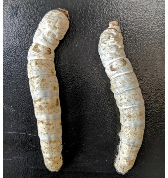
EFFECT OF Momordica charantia AGAINST TYPE 2 DIABETES MODELED IN Bombyx mori
Aarushi Venkatakrishnan
Abstract
Diabetes is a disease that affects millions across the world, occurring when there are high levels of glucose in the blood. Currently, treatments for Type 2 Diabetes include lifestyle and diet changes, medication, and insulin injections; however, natural treatments, such as the vegetable bitter melon, have become more popular in recent years. As it is abundantly grown in Asia, which houses 60% of the world’s diabetics, this finding can be very effective. Using a silkworm model, the hypoglycemic effect of bitter melon was quantified by measuring the silkworm’s hemolymph glucose concentration with the phenol sulfuric acid method. Injections of saline, insulin, and bitter melon solutions were made at the first proleg of the silkworms. Hyperglycemia was induced after two days of a 10% high glucose diet, and human insulin significantly counteracted the effect. There were no changes to mass or length between the hyperglycemic and normal silkworms. After comparing its hypoglycemic effect to insulin, a known hypoglycemic agent, the most effective tested dose of bitter melon was found to be 175 µg/mL, 5 times greater than the corresponding insulin dose, 35 µg/mL. With further trials to determine the symptoms and overall effects to human health, bitter melon can potentially be recommended as an addition to the diet for diabetes treatment.
1.
Background
1.1 Introduction
Diabetes mellitus is a disease which is characterized by high levels of sugar in the blood, hyperglycemia, resulting from the body unable to use blood glucose for energy (Drive, n.d.). Typical symptoms include increased thirst, unexplained weight loss, and frequent infections (Drive, n.d.). This disease occurs when the body is unable to effectively use insulin, a hormone made by the pancreas, to process glucose, and thus causing an increase in blood sugar (“Insulin, Medicines, & Other Diabetes Treatments,” 2016). There are two types ranging in severity: Type 1 and Type 2. Type 1 diabetes is an autoimmune disease in which the immune system destroys islet cells resulting in the body being unable to make insulin (Jin Yang & Mook Choi, 2015). Type 2 diabetes is a chronic condition that changes how the body is able to metabolize glucose, caused by the pancreas either not producing enough insulin or the body becoming resistant to insulin (Matsumoto et al., 2011).
The current treatment for Type 1 is administering insulin exogenically with numerous insulin treatments available, such as an insulin pump, pen, or an inhaler. These vary in terms of how fast they act, the quickest being 15 minutes after injection and the longest being several hours, but correspondingly the duration of the effect differs (“Insulin, Medicines, & Other Diabetes Treatments,” 2016). Type 2 diabetes treatment includes maintaining a healthy lifestyle and monitoring blood glucose levels (Matsumoto et al., 2011). However, Type 2 diabetic patients can even take insulin treatments to make up for that not produced in the body; metformin is a commonly prescribed medicine first given to diabetic patients to lower the amount of glucose
produced by the liver and help the body process insulin better (“Insulin, Medicines, & Other Diabetes Treatments,” 2016).
The number of people being affected by this condition has been increasing rapidly. In 2015, 1.5 million new cases were diagnosed, and in the United States alone, there were 30.2 million Americans with some form of diabetes in 2017 (“CDC Press Releases,” 2016). With this rise, the demand for diabetes treatments has increased. The development of new ways to introduce or stimulate insulin secretion is necessary as it has the potential to help the millions of people afflicted with diabetes live healthier lives.
Although there are a variety of drugs in the market for Type 2 Diabetes, the desire for herbal medicines has increased as they can often be more accessible than traditional forms. In addition, these natural remedies are often more available and accepted than Western Medicine. There has always been a sector of herbal medicines called Complementary and Alternative Medicine (CAM); one of the oldest and most-well known practices is Ayurvedic medicine, which originates in India. Many herbs, fruits, and vegetables used in Ayurvedic medicine have shown promising results against diseases involving high blood pressure, anxiety, cancer, and more (Axe, 2015). One notable vegetable used is Momordica charantia, otherwise known as bitter melon. Numerous studies have been conducted that suggest bitter melon has hypoglycemic effects (Fuangchan, 2011; Jin Yan, 2015).
Jin Yang et al. treated diabetic rats with bitter melon and found three functional components of bitter melon that were likely causing a hypoglycemic effect: charantin, vicine, and polypeptide-p (2015). By using three groups: a high fat control, high fat and 1% bitter melon, and high fat and 3% bitter melon, bitter melon had significantly
improved glucose tolerance and insulin sensitivity. In the 3% bitter melon, they found that it increased the levels of two insulin receptors, (phosphor-insulin receptor substreate-1 (Tyr612) and phosphor-Akt (Ser473), likely stimulating the hypoglycemic effect (Jin Yang & Mook Choi, 2015).
Furthermore, bitter melon has been used in clinical studies using human patients with Type 2 Diabetes. Fuangchan et al. investigated the effects of varying doses of bitter melon (500 mg/day, 1000 mg/day, 2000 mg/day) when comparing it to metformin (1000 mg/day), a current diabetes medication (2011). By measuring the fructosamine concentrations over a 2-week time period from baseline to endpoint, they found that the 500 mg/day and 1000 mg/ day doses did not significantly impact glucose levels, while the 2000 mg/day dose did. When compared to metformin, the effects of bitter melon were still less (Fuangchan, 2011). Both groups did not experience extreme adverse effects; only mild headaches, dizziness, and increased hunger were experienced in the 2000 mg/day bitter melon group (Fuangchan, 2011). The drawbacks of this study include the limited time as it was only conducted for 4 weeks, and because effects were only seen for the 2000 mg/day dose, higher dose levels would need to be tested.
1.2 – Silkworm Model
Although bitter melon is known to have hypoglycemic effects, research surrounding the topic is not standardized and hard to compare. With very minimal clinical trials, the side effects of bitter melon are difficult to determine as well. In Matsumoto et al., scientists established the silkworm as a reliable model of diabetes (Matsumoto et al., 2011). While silkworms do not have blood like humans, they have hemolymph which is a fluid “equivalent” to blood. In this study, glucose levels after treatment with a high glucose diet were higher than that of the silkworms fed a normal diet. By treating the hyperglycemic silkworms with insulin, glucose levels returned to normal. Moreover, they also tested an herbal extract, jiou, and found that it could mimic the effects of insulin by reducing glucose concentrations.
Based on this research, the silkworm model could be used to determine the hypoglycemic effects of bitter melon. Here we show hyperglycemic silkworms that are treated with bitter melon extract, to study if their hemolymph sugar levels will go down without adverse reactions in terms of body size, body mass, or lifespan because bitter melon has been known to have hypoglycemic properties as used in ayurvedic medicine. This hypoglycemic effect is likely as bitter melon has the identified components charantin, vicine, and polypeptide-p and has been a cultural remedy as used in Ayurvedic medicine.
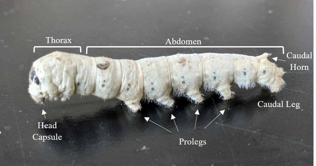
1. Anatomy of a silkworm. Length measurements were made from the thorax to the caudal leg. Injections were made in between the first proleg and the second proleg from the head capsule.
2. Methods
This study consisted of two preliminary experiments and two main experiments. The two preliminary experiments determined the equation for the Beer’s Law Plot to be used when calculating the D-glucose concentration of silkworms and established that a high glucose diet raised the D-glucose levels of silkworms. The main experiments tested the effect of insulin when compared to the same dose of bitter melon and evaluated the optimal concentration of bitter melon. The experiment unit was the addition and kind of hypoglycemic agent, measuring the change in average D-glucose levels. For the main experiments, the positive control was the hyperglycemic silkworm treated with insulin, a known hypoglycemic agent. The negative control was the silkworm fed a normal diet and injected with saline, to mimic the effect of an injection without the addition of a chemical agent.
2.1 – Silkworm Diet
The essentials of the silkworm diet consist of mulberry leaves. To create the silkworm diet, Carolina® Silkworm Diet was purchased from Carolina Biological. In a 2000 mL glass beaker, ½ pound of the mulberry powdered diet was added to 720 mL (roughly 3 cups) of tap water. Using a stirring rod, the substances were thoroughly mixed to a uniform consistency. It was then covered with plastic wrap and secured with a rubber band. The beaker was placed in the microwave at high heat until the mixture came to a boil, usually after 1-2 minutes. This caused the mixture to rise and bubbles appeared on the surface. Once the mixture boiled, the beaker was removed from the microwave and stirred to again ensure uniform consistency. It was then placed back in the microwave to repeat the process. After the second boil and mixture, plastic wrap was tightly placed against the surface of the mixture to ensure no moisture escaped. Time was allowed for the beaker and substances to cool down. Then, the top of the beaker was secured with plastic wrap and a rubber band. It was placed in the
Figure
2.2 – Silkworm Maintenance
Silkworm eggs were purchased from Carolina Biological. They were placed in petri dishes and incubated at 29 °C. After roughly a week, the eggs hatched, and they were disposed of. The larva was transferred to a fresh plate with mulberry powdered diet placed on a paper towel. Feedings were made every other day to clean out feces and remove dried food. The experiment was performed during the fifth instar (around 4 weeks after hatching). Raising the temperature increased growth, whereas lowering the temperature delayed growth.
2.3 – High Glucose Diet
To induce hyperglycemic conditions, a high glucose diet of the Mulberry Chow was created by mixing appropriate amounts of D-Glucose and the Mulberry Chow. D-Glucose was added to the Mulberry Chow in a beaker, and then mixed until all contents were dissolved. A 10% and 15% D-Glucose diet were created.
2.4 – Injection
50 µl of each solution was injected into the hemolymph at the second abdominal segment of the larva after the first proleg using 1 mL syringes (Fig. 2). Injections were done on 12-hour cycles for 2 days after 2 days of the high glucose diet for the preliminary experiments. Injections were performed once 24 hours before extraction for the main experiments. The total treatment lasted 4 days with measurements taken on Day 5.
was made with 0.9% NaCl and 0.1% acetic acid. A stock solution of bitter melon was created by combining 0.50 grams of powdered bitter melon with 50 mL of distilled water to make a 0.1 g/mL solution. It was heated at 40 °C, for 15 minutes and left overnight for 2 days. Then, vacuum filtration was performed 3 times to filter out particulates. It was then appropriately diluted to the varying concentrations used in the experiment.
2.6 – Glucose Quantification
Hemolymph was collected from the larvae through a cut on the first proleg after they had developed to the fifth instar. Precipitated proteins were removed by centrifugation at 3000 rpm for 10 min. 175 µl of the supernatant was diluted with 175 µl distilled water for sugar quantification (350 µl total). The total sugar in the hemolymph was determined using the 0.05 % phenol-sulfuric acid (PSA) method. Hemolymph extract (350 µl) was mixed vigorously with 1050 µl 70% sulfuric acid. Immediately, 210 µl of 5% phenol aqueous solution were added and mixed. The test tubes were held in a water bath at 90 °C. The samples were then cooled to room temperature. The absorbance at 490 nm was measured using a spectrophotometer. Serially diluted glucose solution was used as a standard.
2.7 – Statistical Measurements
Measurements of the mass (g) and length (cm) of the silkworms were taken prior to experimentation. They were then monitored throughout the trial days and recorded until extraction. Data were analyzed using unpaired student t-tests with unequal variance, as sample size differed across the trials. Error bars were calculated using standard error of the mean (SEM).
2.8 – Comparing the Effects of Insulin and Bitter Melon
To determine whether bitter melon has hypoglycemic effects, a silkworm model was used as it has been previously identified as a workable model for diabetes research (Fuangchan, 2011). Three characteristics were measured to determine the effectiveness of the bitter melon treatment: body mass, body length, and hemolymph sugar levels. Each trial consisted of 6 treatments, separated into high-glucose and normal diet models. In addition to these treatments, the effect of insulin on both the hyperglycemic and normal silkworm was used to provide a standard of comparison to see the success of the bitter melon extract (Table 1.1).
2.5
– Injection Solutions
A 35 µg/mL solution of insulin was created by diluting a 20 mg/mL solution to 15 mL. The dilution solution
Figure 2. Injection site after the first proleg. Hemolymph was extracted from this same site as well.
Saline “Normal” with Saline (NS) “High” with Saline (HS)
Insulin “Normal” with Insulin (NI) “High” with Insulin (HI)
Bitter Melon “Normal” with Bitter Melon (NB) “High” with Bitter Melon (HB)
2.9 – Determining the Ideal Concentration of Bitter Melon
Following the experimental model from the Injections, varying concentrations of bitter melon were tested in the silkworms to determine which concentration of bitter melon has the largest effect on the sugar concentration in silkworms (Table 1.2).
Table 1.2. Experimental design comparing effect of varying doses of bitter melon Diet
Treatment Normal Diet High Glucose Diet
Saline “Normal” with Saline (NS) “High” with Saline (HS)
Insulin - “High” with Insulin (HI)
Bitter
Melon 1 - “High” with Bitter
Bitter
Melon 1 (HB1)
Melon 2 - “High” with Bitter
Bitter
Melon 2 (HB2)
Melon 3 - “High” with Bitter
Melon 3 (HB3)
3. (A, B) Glucose standards undergoing phenolaqueous protocol and depicted visually with a gradient of yellow colors, shown from left to right as (1) Blank, (2) 1.00 M D-Glucose, (3) 0.055 M D-Glucose, (4) 0.0275 M D-Glucose
3.2 – High Glucose Diet
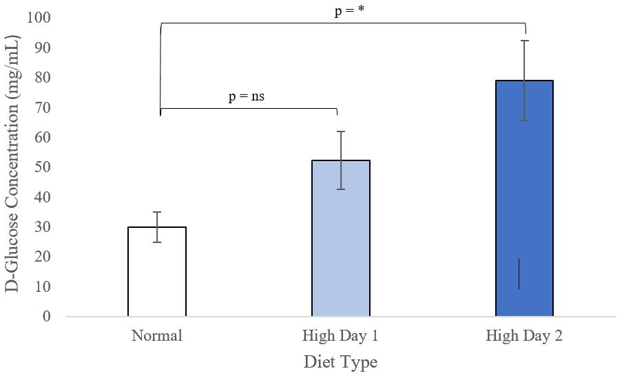
Before proceeding with the experiment, a baseline of a high glucose diet needed to be tested. In this preliminary experiment, three treatments were tested: a normal diet of mulberry chow, a 10% glucose diet after 24 hours, and the same diet after 48 hours. A sample size of 9 silkworms was used for the normal diet. Five silkworms were used for both of the 10% glucose diet treatments. Average glucose levels across the hemolymphs of the silkworms are shown (Fig. 4).
3. Results
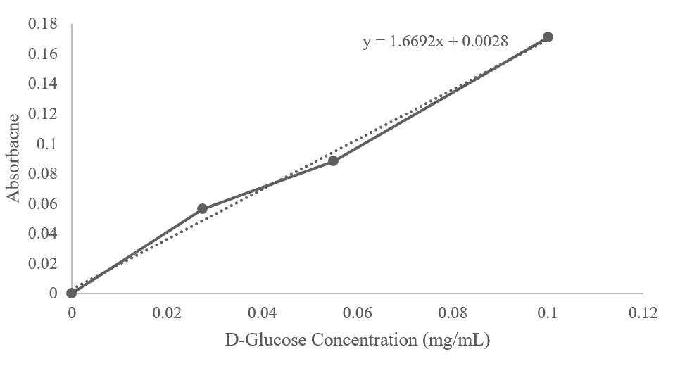
3.1 – Glucose Quantification
To understand and best utilize the phenol aqueous method, a series of D-glucose standards were used to create a Beer’s Law plot (Fig. 3A,B). Different D-Glucose concentrations were used to generate a standard. These included 0.0275 M, 0.055 M, and 1.000 M.
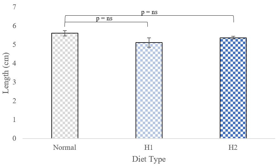
Figure
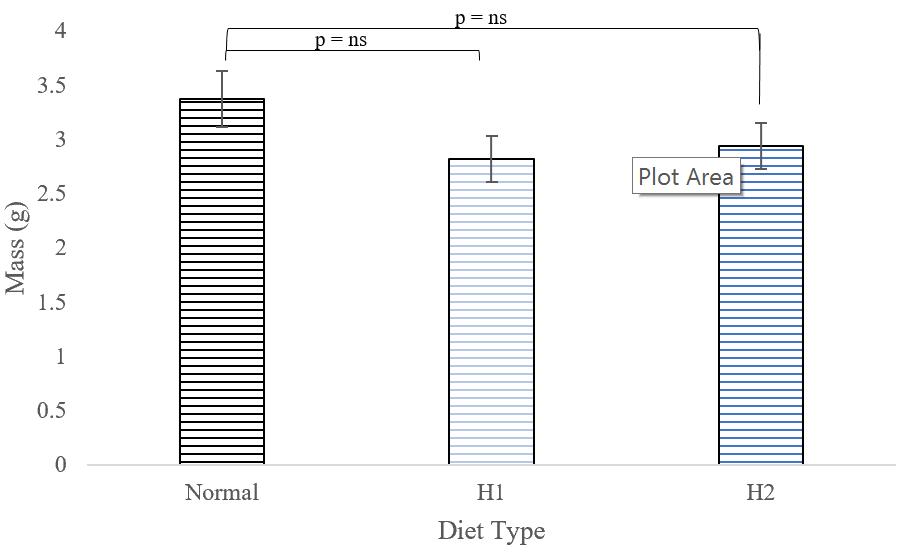
Figure 4. (A) Average D-glucose concentration. (B) Average mass. (C) Average length. Three different treatment groups were measured: Normal (mulberry diet); High Day 1 (mulberry + 10% glucose for 24 hours); High Day 2 (mulberry to 10% glucose for 48 hours). (p < 0.05= *, p < 0.01= **, p < 0.001 = ***, p > 0.05= ns). Error bars ± SEM.
The average glucose concentration of a normal silkworm is about 30.0 mg/mL (Fig. 4A). With the addition of a high glucose diet, the average glucose concentration is 52.4 mg/mL after one day and 79.1 mg/mL after two days. This means that after 48 hours, there is almost a 2.5-fold increase. After conducting a t-test for further statistical analysis, p-values were calculated. The only statistically significant difference is between the normal diet and two days of the high glucose diet, indicating that 48 hours at a minimal of 10% D-glucose diet is required to increase hemolymph glucose levels significantly. There was no statistically significant difference between the mass and length of the normal silkworms and the two tested trials (Fig. 4B and 4C).
3.3 – Comparing the Effects of Insulin and Bitter Melon
After establishing that a hyperglycemic diet could induce high glucose concentrations in silkworms, the effect of insulin was tested on a normal and high glucose diet. This standard concentration would also be replicated by an equal dose of bitter melon extract. Based on the results of the previous experiments, silkworms were fed a high glucose diet for 2 days to induce hyperglycemia (Fig. 4). On Day 3 of the diet, injections were performed with the various treatments. Then, on Day 4, their hemolymphs were extracted and quantified for glucose concentration.
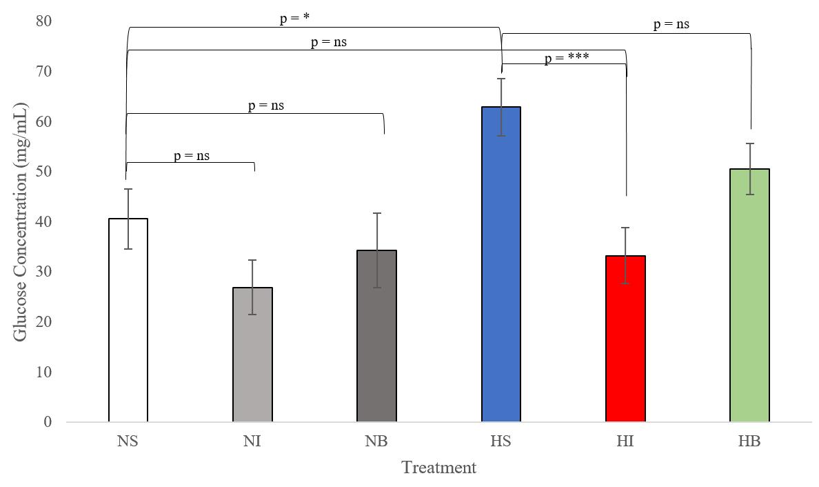
Figure 5. Average glucose concentrations across various treatments. Six different treatment groups were measured: Normal with Saline (mulberry diet + insect saline, n=8), Normal with Insulin (mulberry diet + 35 µg/mL insulin, n=7), Normal with Bitter Melon (mulberry diet + 35 µg/mL bitter melon extract, n=9), High with Saline (mulberry diet + 15% glucose for 84 hours + insect saline, n=9), High with Insulin (mulberry diet + 15% glucose for 84 hours + 35 µg/mL insulin, n=10), and High with Bitter Melon (mulberry diet + 15% glucose for 84 hours + 35 µg/mL bitter melon extract, n=9). (p < 0.05= *, p < 0.01= **, p < 0.001 = ***, p > 0.05 = ns). Error bars ± SEM.
The average glucose concentration for each of the treatments are as follows (Fig. 5): 40.595 mg/mL (Normal diet with Saline), 26.929 mg/mL (Normal diet with 35 µg/mL Insulin), 34.366 mg/mL (Normal diet with 35 µg/ mL Bitter Melon), 62.905 mg/mL (15% High glucose diet with Saline), 33.287 mg/mL (15% High glucose diet with Insulin), and 50.579 mg/mL (15% High glucose diet with bitter melon). As can be seen from the p-values, there was a statistically significant difference between the normal with saline and high with saline, and one between the high with saline and high with insulin. This corresponds to the predicted control values. There was no statistically significant difference between the high with saline and high with bitter melon.
3.4 – Revised Standard Curve
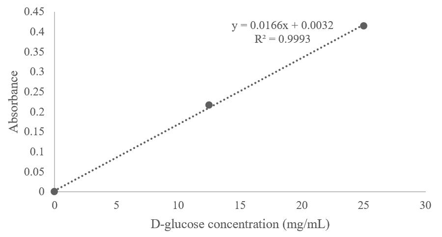
Using a different series of D-glucose solutions and a new spectrophotometer, a new standard curve was created (Fig. 6).
Figure 6. New Glucose Standard Curve. Using concentrations of 12.5 mg/mL and 25 mg/mL, the standard curve for glucose was created.
The linear fit was used to evaluate the following experiment in terms of finding the ideal dose of bitter melon for hyperglycemic silkworms.
3.5 – Determining the Ideal Concentration of Bitter Melon
Ultimately, a 35 µg/mL concentration of bitter melon was not effective, but it did show a decrease from the hyperglycemic silkworms (Fig. 5). By adjusting the concentration of bitter melon, the downward trend could be quantified further.
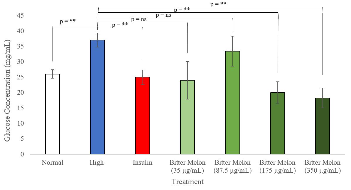
The average values for each treatment were: 26.046 mg/mL (Normal with Saline), 37.111 mg/mL (15% High glucose diet with Saline), 25.043 mg/mL (15% High glucose diet with 35 µg/mL Insulin), 24.029 mg/mL (15% High glucose diet with 35 µg/mL Bitter melon), 33.459 mg/mL (15% High glucose diet with 87.5 µg/mL Bitter melon), 20.006 mg/mL (15% High glucose diet with 175 µg/mL Bitter melon), and 18.265 mg/mL (15% High glucose diet with 350 µg/mL bitter melon) (Fig. 7A).
Insulin significantly reduced the glucose concentrations of the high glucose diet to the levels of the normal diet. Two bitter melon treatments yielded statistically significant results, with the 175 µg/mL bitter melon extract having a p-value that most closely resembled insulin (0.00303 and 0.002954).
Figure 7. (A) Determining a Statistically Significant Bitter Melon dose. Seven different treatment groups were measured: Normal with Saline (mulberry diet + insect saline, n=8), High with Saline (mulberry diet + 15% glucose for 84 hours + insect saline, n=9), High with Insulin (mulberry diet + 15% glucose for 84 hours + 35 µg/mL insulin, n=7, High with 35 µg/mL Bitter Melon (mulberry diet + 15% glucose for 84 hours + 35 µg/mL bitter melon extract, n=5), High with 87.5 µg/mL Bitter Melon (mulberry diet + 15% glucose for 84 hours + 87.5 µg/mL bitter melon extract, n=8), High with 175 µg/mL Bitter Melon (mulberry diet + 15% glucose for 84 hours + 175 µg/mL bitter melon extract, n=6), and High with 350 µg/mL Bitter Melon (mulberry diet + 15% glucose for 84 hours + 350 µg/ mL bitter melon extract, n=5). (p < 0.05= *, p < 0.01= **, p > 0.05 = ns). Error bars ± SEM. (B) (Left) 350 µg/ mL bitter melon diet fed silkworm exhibiting a yellowish color and less rigid than (Right) Normal diet fed silkworm.
4. Discussion
4.1 – Bitter Melon’s Effect on Hyperglycemia
The results confirm Matsumoto et al.’s conclusion that a silkworm model can exhibit hyperglycemia (Fig. 4). By feeding a 10% glucose mulberry diet, the hemolymph sugar levels increased significantly. For the convenience of the model, the addition of glucose was increased to 15% to
B.
ensure that the intake across samples would be the same and that the effect was the greatest. Additionally, this figure also examines the mass and length across treatments. Matsumoto et al. claimed that mass and length differed with the addition of glucose to the diet, however, no significant variation in these metrics were found, indicating these metrics were not good indicators of health (2011).
From there, insulin was added as a control treatment to compare the effect of bitter melon. The 35 µg/mL was appropriately scaled by the average insulin treatment for humans, with guidance from Matsumoto et al. (2011). There was a significant decrease in glucose levels, again confirming the silkworm model. New treatments were tested with a 15% glucose mulberry diet instead of the 10% glucose mulberry diet (Fig. 4 & Fig. 5). With an equal concentration of bitter melon, 35 µg/mL, there was no significance in the data (p = 0.12). However, bitter melon did reduce the glucose levels from the high glucose and saline sample. From this, it could be concluded that bitter melon requires a larger dose than insulin does to perform a hypoglycemic effect.
This prediction was tested (Fig. 7). With four varying concentrations of bitter melon – 35 µg/mL, 87.5 µg/ mL, 175 µg/mL, and 350 µg/mL – the relationship of bitter melon doses and the hypoglycemic effect were discovered. The most effective dose out of the trials was 175 µg/mL bitter melon, as it produced a similar p-value to the insulin treatment. However, the trend created with increasing doses did not suggest a linear trend, like predicted. Instead, it presented with a curved shape that is likely because of small sample size. The sample sizes of the various treatments ranged from 5 to 9, indicating that more samples would be necessary to determine if a linear trend exists.
4.2 – Limitations
Although the metrics of mass and length were not appropriate in quantifying the effect of bitter melon, qualitative observations of behavior helped define the health when compared to normal silkworms. With a high glucose mulberry diet, silkworms appeared lethargic and did not move as fast or eat as much as the normal diet silkworms. This could speak to food aversion or a toxicity of glucose in the diet. Silkworms have been frequently studied as a model of toxicity as they lack an adaptive immune system (Chen & Lu, 2018). They possess PGs and LPS, immune stimulators that silkworms have developed based on their cell walls (Chen & Lu, 2018). This allows silkworms to defend against pathogens and infections. If they had a similar response to the insulin or glucose diet, the model would not be ideal to study. With the addition of insulin, the worms were still slightly affected by this effect. In addition, silkworms in the bitter melon trials exhibited a yellowish tinge (Fig. 7B). The higher the dose, the higher
the mortality rate. The study consisted of trials with 10 initial worms, however, the sample sizes are significantly lower for the 35 µg/mL trial and the 350 µg/mL trial, as only 50% of the silkworms in those trials survived (Fig. 7A).
In addition, the administration of treatment also impacted the survival rate of the silkworms. As they have a limited hemolymph volume, injections caused severe hemolymph loss. Bruises and strain along the head and thorax were very visible. With extra pressure from the injections, silkworms often refrained from eating as they could not perform movement. This method of administering was rather ineffective as many samples could not be used for analysis.
Lastly, the spectrophotometer used for the first half of the experiment was heavily used and therefore yielded unpredictable results. Therefore, results from the first part (Fig. 2 and 3) cannot be compared to results from the second part (Fig. 5), as there were two new standard curves created. Overall, similar results were yielded throughout the trials, which allows the general effect of the treatments to be compared.
5. Conclusion and Future Work
By using a silkworm model, diabetes could be effectively modeled. The most effective dose of bitter melon was determined to be 175 µg/mL, which had effects that closely resembled those of the insulin treatment. The data do not confirm a linear relationship between dose of bitter melon and hypoglycemic effect, as there was variation in the data. With this knowledge, future work is necessary before bitter melon can be marketed as a hypoglycemic agent. At this dose, side effects and symptoms should be generated to understand how it would impact human health. This can be done through mice and human clinical trials. Additionally, different methods of preparing the extract should be performed. A liquid extract was prepared with distilled water and a powdered form of bitter melon to make the injection solutions in the previously mentioned trials. The difference between powdered and fresh bitter melon should be studied, with the different parts of bitter melon as well (the core and the exterior). With the combination of all of these factors, the doses may vary depending on what is optimal.
Bitter melon does not only show potential as a hypoglycemic agent, but also as a potential cancer and osteoarthritis therapy (Raina, 2016; Soo May, 2018). Guided by bitter melon’s targeted effect against Type 2 Diabetes, Raina et al. attempted to provide a comprehensive view of the bioactivity of bitter melon’s different components and determine if they are applicable to cancer treatment (Raina et al., 2016). Specifically, they focus on how bitter melon interacts with other drugs. This is an important aspect to consider concerning
diabetes as well, to see how bitter melon interacts with the mechanisms of insulin (Raina et al., 2016). Soo May et al. focus on bitter melon’s anti-inflammatory effects and how they can potentially reduce knee pain in osteoarthritis patients (Soo May et al., 2018). They concluded that with 3 months of supplementation, bitter melon can reduce the need for analgesia consumption, while also showing reductions in body weight, body mass index, and fasting blood glucose (Soo May et al., 2018). Overall, bitter melon has a variety of beneficial effects that are not well studied, so it is important to understand how it affects the body to better recommend this natural remedy.
Once this has been completed, health care providers can use this information, especially in Asian countries, to inform their patients about additional foods to include into their diet, with the appropriate intake. As there are many different vegetables and roots that are said to exhibit this hypoglycemic effect, they can be tested similarly to how it has been done in this paper and examine the effects before formally recommending inclusion into the diet.
6. Acknowledgments
I would like to thank Dr. Kimberly Monahan for being an encouraging mentor and guiding me through the research process. Thank you to the Research in Biology class of 2019 for providing support throughout this project. Thank you to Kevin Zhang and Tyler Edwards for being my lab assistants over the summer. Finally, I would like to thank Dr. Sheck, the North Carolina School of Science and Mathematics, and the Glaxo Endowment for allowing me the opportunity to experience research.
7. References
Axe, J. (2015, August 29). 7 Benefits of Ayurvedic Med icine: Lower Stress, Blood Pressure & More. (n.d.). Retrieved September 22, 2018, from https://draxe.com/ ayurvedic-medicine/
CDC Press Releases. (2016, January 1). Retrieved January 27, 2018, from https://www.cdc.gov/media/ releases/2017/p0718-diabetes-report.html
Chen, K., & Lu, Z. (2018). Immune responses to bacterial and fungal infections in the silkworm, Bombyx mori. Developmental & Comparative Immunology, 83, 3–11. https:// doi.org/10.1016/j.dci.2017.12.024
Drive, A. D. A. 2451 C., Arlington, S. 900, & Va 22202 1-800-Diabetes. (n.d.). Diabetes Symptoms. Retrieved October 26, 2018, from http://www.diabetes.org/ diabetes-basics/symptoms/
Fuangchan, A. (2011) Hypoglycemic effect of bitter melon compared with metformin in newly diagnosed type 2 diabetes patients. Journal of Ethnopharmacology, 134(2), 422–428. https://doi.org/10.1016/j.jep.2010.12.045
Insulin, Medicines, & Other Diabetes Treatments. (2016, November 01). Retrieved January 27, 2018, from https:// www.niddk.nih.gov/health-information/diabetes/ overview/insulin-medicines-treatments
Jin Yang, S., Mook Choi, Jung. (2015). Preventive effects of bitter melon (Momordica charantia) against insulin resistance and diabetes are associated with the inhibition of NF-κB and JNK pathways in high-fat-fed OLETF rats.
The Journal of Nutritional Biochemistry, 26(3), 234–240. https://doi.org/10.1016/j.jnutbio.2014.10.010
Matsumoto, Y., Sumiya, E., Sugita, T., & Sekimizu, K. (2011). An Invertebrate Hyperglycemic Model for the Identification of Anti-Diabetic Drugs. PLOS ONE, 6(3), e18292. https://doi.org/10.1371/journal.pone.0018292
Raina, K., Kumar, D., & Agarwal, R. (2016). Promise of bitter melon (Momordica charantia) bioactives in cancer prevention and therapy. Seminars in Cancer Biology, 40–41, 116–129. https://doi.org/10.1016/j. semcancer.2016.07.002
Soo May, L., Sanip, Z., Ahmed Shokri, A., Abdul Kadir, A., & Md Lazin, M. R. (2018). The effects of Momordica charantia (bitter melon) supplementation in patients with primary knee osteoarthritis: A single-blinded, randomized controlled trial. Complementary Therapies in Clinical Practice, 32, 181–186. https://doi.org/10.1016/j.ctcp.2018.06.012
TETRAETHYL
ORTHOSILICATE-POLYACRYLONITRILE HYBRID MEMBRANES AND THEIR APPLICATION IN REDOX FLOW BATTERIES
Ethan Frey
Abstract
Redox flow batteries (RFBs) are a reliable solution to long term energy storage, but lack an inexpensive and effective proton exchange membrane. Polyacrylonitrile (PAN) nanoporous membranes have a high chemical stability but low hydrophilicity when compared to Nafion, the standard membrane. The addition of tetraethyl orthosilicate (TEOS) increases the mechanical and thermal properties of membranes and may also increase their hydrophilicity due to the presence of hydrophilic silicon hydroxide bonds. Therefore, doping a nanoporous hydrophobic PAN membrane with TEOS is hypothesized to increase the hydrophilicity of the membrane, while still maintaining a high chemical stability and low vanadium crossover. Membranes of Nafion 212, nanoporous PAN, and a nanoporous hybrid TEOS/PAN were prepared through a phase inversion method and tested for chemical stability, proton and vanadium crossover in a model RFB, and water contact angle. The TEOS/PAN hybrid membrane had a higher hydrophilicity than both PAN and Nafion. The addition of TEOS had no impact on chemical stability. However, the TEOS/PAN hybrid membrane did have a higher vanadium crossover and lower proton/vanadium selectivity. It was concluded that TEOS can increase hydrophilicity, but more research needs to be done to improve proton/vanadium selectivity, potentially by optimizing pore size. Since TEOS was proven as an effective additive to membranes, progress was made towards the development of an ideal proton exchange membrane and a solution to long-term energy storage.
1. Introduction
Recently, polyacrylonitrile (PAN) nanofiltration membranes have proven to be a promising alternative to Nafion membranes due to their high chemical stability, and inexpensive cost. However, PAN membranes have been found to lack the proton conductivity of Nafion, a property that could be increased through the addition of additives to a PAN membrane. The addition of tetraethyl orthosilicate to a PAN membrane may not only increase the hydrophilicity and proton conductivity of PAN, but also improve the membrane’s mechanical strength and thermal properties, while still maintaining the chemical stability of PAN. The creation of a hybrid membrane of PAN and TEOS could make progress towards the creation of a cheaper membrane with properties comparable to that of Nafion.
As renewable energy has become increasingly popular, demand for long term energy storage increased as well. As a result, a lot of attention has been given to redox flow batteries (RFBs) due to their ability to store energy for an indefinite period of time. What differentiates a RFB from other battery types is that it behaves essentially as a reversible fuel cell.
Design: Two different oxidation states of vanadium are stored in the tanks on either side of the battery and pumped into two adjacent half cells where the vanadium is reduced or oxidized and a flow of electrons is created. However, a proton exchange membrane is essential to allow this reaction to occur.
The fuel is stored in tanks separate from where the oxidation and reduction occurs (Fig. 1). This fuel is pumped into two adjacent half cells separated by a proton exchange membrane. The vanadium on one side of the half cell is reduced and the other side is oxidized before being pumped back into the fuel tank. The battery is finished charging or discharging when all of the fuel has been reduced or oxidized. Commonly used batteries, such as lithium-ion batteries, can slowly discharge while not in use, resulting in a loss of charge over time. This is due to the fuel being stored where the reduction and oxidation occurs, allowing spontaneous reactions to take place even
Figure 1. Redox Flow Battery
when the battery is not in use. Since the fuel in RFBs is stored externally, the battery cannot slowly discharge over time while not in use, and energy can be stored for an indefinite period of time. Vanadium is most typically used in RFBs due to its multiple oxidation states and large ion size (Alotto et al., 2014).
The expensive proton exchange membrane prevents the use of RFBs on a commercial scale. The most widely used membrane is Nafion. This membrane is expensive and its properties could still be improved upon. It still exhibits vanadium ion crossover, and a higher hydrophilicity and proton conductivity could increase its efficiency. However, it is challenging to manipulate these properties while still maintaining a high level of chemical stability. Vanadium ion crossover is difficult to decrease while still maintaining proton conductivity. Similarly, proton conductivity is difficult to increase without decreasing chemical stability or increasing vanadium crossover. A membrane must be both hydrophobic to maintain chemical stability and hydrophilic to conduct protons. An alternative is to create a membrane that is simply very hydrophobic and has nanopores to allow protons to pass through. However, an extremely hydrophobic membrane struggles to keep the nanopores big enough to allow protons to pass through but small enough to prevent vanadium crossover. Nafion is designed (Fig. 2) such that it has a fluorinated carbon chain that allows for high chemical stability and hydrophobicity. Yet, Nafion still has a S-OH bond that allows for some hydrophilicity.
Figure 2. Nafion Structure: Nafion contains a hydrophobic fluorinated backbone with a hydrophilic sulfur hydroxide bond.
As a result of its structure, Nafion maintains a high chemical stability while still allowing protons to cross over the membrane. The cost of Nafion is mainly due to the manufacturing cost of making fluorinated membranes. Therefore, non-fluorinated membranes have been investigated as a cheaper alternative. However, many lack the chemical stability of fluorinated membranes, which poses a challenge for their application in vanadium RFBs. Polyacrylonitrile has recently been recognized as a promising option for non-fluorinated membranes due to its high chemical stability despite the absence of fluorine. In fact, PAN has been explored in applications as a superhydrophobic polymer with a water contact angle
exceeding 170°, indicating its high chemical stability (Feng et al., 2002). However, high hydrophobicity can become problematic when it prevents the membrane from conducting protons. Polyacrylonitrile membranes with nanopores from a phase inversion method (Zhang et al., 2011) and conditioning in an alkali solution (Karpushkin et al., 2017) have been investigated. These investigations found that, as expected, polyacrylonitrile lacks the proton conductivity of Nafion. Therefore, doping PAN to increase its hydrophilicity could create a membrane that is comparable to Nafion.
Doping Nafion with metal oxides to improve its hydrophilicity has been explored repeatedly and proven successful (Noto et al., 2007). Specifically, silicon dioxide has been proven effective due to its ability to significantly increase the thermal properties and hydrophilicity of Nafion (Yu et al., 2007). Doping PAN with metal oxides should also increase its hydrophilicity. Tetraethyl orthosilicate (TEOS) has been explored as an additive to a polyvinylidene fluoride membrane (Liu et al., 2008). However, only the enhanced mechanical properties and effect on pore size were explored and the doped PVDF membrane was not tested in application for RFBs. TEOS has also been tested and used for the creation of a super hydrophilic surface in photovoltaic cells, proving its use as a hydrophilic material (Yan et al., 2015). Its hydrophilicity is due to the presence of hydroxide bonds after being polymerized and hydrolyzed, like the ones in Nafion (Fig. 3).
Figure 3. Hydrolyzed and Polymerized TEOS: Just like Nafion’s hydrophilic sulfur hydroxide bonds, TEOS contains hydrophilic silicon hydroxide bonds.
Doping PAN with TEOS should have the same effect that adding a metal oxide, like silicon oxide, would have. TEOS has also demonstrated an increase in the thermal stability of membranes (Liu et al., 2008). Therefore, doping PAN with TEOS should combine the superhydrophobicity and chemical stability of PAN with the super-hydrophilicity, thermal stability, and high tensile strength of TEOS without compromising the high chemical stability or proton/vanadium selectivity of PAN. Engineering a more efficient and less expensive proton exchange membrane will allow energy to be generated and stored for an indefinite period of time, making
renewable energy much more reliable and allowing entire cities to depend on it. The future of RFB membranes lies in the development of a non-fluorinated membrane, due to the cheaper manufacturing cost. Through testing how to improve the properties of a promising non-fluorinated membrane, progress is made towards engineering an ideal proton-exchange membrane.
2. Methods
2.1 – Preparing the Membranes
The following procedure was adapted from Liu (2008). The nanoporous PAN membrane was prepared by casting a 15 wt% PAN (Mw = 150,000), 3 wt% LiCl, and 4 wt% polyvinylpyrrolidone (PVP) solution in DMSO on a glass plate and leveling it with an RDS40 wire round rod (RD Specialties, USA). A normal phase inversion was then conducted using a water bath at room temperature. The membrane was left in the water bath for 1-2 days to remove any remaining solvents. The hybrid membrane was prepared by lowering the weight percentages to 12.5 wt% PAN, 2.5 wt% LiCl, 3.25 wt% PVP, and adding 6.7 wt% TEOS. A normal phase inversion was then conducted in an acid bath (pH = 1), to allow the polymerization of TEOS, and then transferred to a water bath for 1-2 days.
2.2 – Model Redox Flow Battery
The model redox flow battery was designed using two mini-variable flow peristaltic pumps (Fisher) and a modified fuel cell (Heliocentris). The fuel cell was composed of graphite, two carbon felt electrodes, and a membrane. The design is shown below (Fig. 4).
4. Model Redox Flow Battery Design: The design consists of two peristaltic pumps, two fuel tanks, and two adjacent half cells with electrodes separated by a membrane.
2.3 – Vanadium 4+ Preparation
All fuel was prepared through the reduction of V2O5 to VO2+ using glycerol in the presence of HCl (Small et al., 2017). 38.9 mL of deionized water, 50.0 mL of 12.1M HCl, and 5.0g of V2O5 was added to a beaker and stirred at
60-90°C. After the dissolution of V2O5, temperature was maintained while .7mL of glycerol was stirred in. Once a uniform blue color was obtained, indicating the formation of V4+, the reaction was completed.
2.4 – Proton/Vanadium Selectivity Test
Proton vanadium selectivity was tested by filling one side of the fuel cell with water and the other side with 2M VO2+ and 7M HCl. The pumps were run for 45 minutes with samples being taken every 5 minutes. The concentration of vanadium in these samples was measured using a spectrophotometer. The absorption at 765nm was measured and Beer’s law was used to calculate the concentration using a molar absorptivity of 13.40 (Choi et al., 2013). The concentration of protons was measured through pH measurement using a pH meter (Vernier). All data were recorded in LoggerPro (Vernier).
2.5 – Chemical Stability
The chemical stability of the membranes was estimated by placing the membranes in a solution that consisted of 1M V2O5 and 5M HCl at 50°C for 30 days. The presence of VO2+ indicated that the membrane had been oxidized. The stability of the membrane was determined by calculating the percentage of VO2+ in the sample in comparison to a control solution without a membrane.
3. Results
3.1 – Water Contact Angle
Figure 5. Water contact angle of a drop of water on the membranes. The photo was taken on an IPhone 6s and the angles were measured using Logger Pro. (A) Nafion (B) PAN (C) Hybrid
Figure
Hydrophilicity of Nafion, PAN, and the hybrid membrane was demonstrated by measuring the contact angle of a water droplet (Fig. 5). It was found that Nafion had the largest water contact angle of 87.09° followed by PAN at 55.01° and the hybrid membrane at 42.27°.
membrane the highest (Fig. 6A). The TEOS/PAN hybrid membrane also had the highest proton conductivity (Fig. 6B). The overall proton/vanadium selectivity was similar for the Nafion and PAN membranes. However, the hybrid membrane had a much lower selectivity (Fig. 6C).
3.3 – Chemical Stability
Table 1. The percent of V5+ reduced to V4+.This indicated ongoing oxidation of the membrane and therefore can be used to analyze the chemical stability of the membrane. Concentrations were measured using a spectrophotometer.
Percent Reduced Compared to reference 96.06% -49.94% -30.54%
The chemical stability of the prepared membranes was measured as the percent of the original vanadium that was reduced (Table 1), indicating ongoing oxidation of the membrane. The percent of vanadium reduced was highest for Nafion with 4.72% followed by the hybrid membrane with 1.67% and the PAN membrane with 1.20%. However, 2.41% of the vanadium in the reference sample (the sample without a membrane) was reduced. When comparing the measured percentages to the reference percentages, it is found that the percent reduced in the Nafion was 96% higher than that of the reference sample, PAN was 49.9% smaller, and the hybrid was 30.5% smaller.
4. Discussion and Conclusion
The vanadium and proton crossovers were measured over a 45 minute period. A model redox flow battery was used. An acidic V4+ solution was placed on one side of the battery and deionized water on the other side. The concentration of vanadium was measured over time using a spectrophotometer and the proton concentration was measured using a Vernier pH probe. The proton/ vanadium selectivity was determined as the ratio of the proton crossover to the vanadium crossover.
Nafion was found to have the lowest vanadium crossover, PAN the second highest, and the hybrid
The goal of this project was to demonstrate that hydrolyzed and polymerized TEOS could effectively increase hydrophilicity and provide a suitable substitute for Nafion in a vanadium redox flow battery. The results of the experiments are summarized in Table 2. Introducing TEOS to the PAN membrane improved its hydrophilicity as demonstrated by the water contact angle test (Fig. 5). The smaller the water contact angle, the more hydrophilic the material, because the water is not as repelled to the polymer. The hybrid membrane had a smaller water contact angle than both PAN and Nafion, indicating a high hydrophilicity. Its high hydrophilicity was further demonstrated when tested in a model redox flow battery. The hybrid membrane showed a higher proton crossover than both Nafion and PAN (Fig. 6). These tests show that the proton conductivity of the PAN membrane was most likely successfully increased. The chemical stability of
Table 2. Data Summary: The water contact angle, vanadium crossover, proton crossover, proton/vanadium selectivity, and chemical stability of Nafion, PAN, and the hybrid TEOS/PAN membrane. Water
the membrane was also maintained with the addition of TEOS, as none of the membranes had a significant amount of oxidation occur in the presence of a strong oxidizer. However, the TEOS-PAN hybrid did show increased vanadium crossover. Prevention of vanadium crossover is an essential function of a proton-exchange membrane. The different oxidation states of vanadium on either side of the membrane need to remain unmixed while still allowing protons to cross over. Therefore, proton/vanadium selectivity is measured as the ability of the membrane to allow protons to cross over but prevent vanadium ions from crossing over. A higher proton/vanadium selectivity is ideal. However, the hybrid membrane displayed a lower proton/vanadium selectivity than both Nafion and the PAN membrane. Further optimization will need to be performed in order to improve proton/vanadium selectivity.
There are several areas that can be explored to improve upon this research. The PAN and TEOS-PAN membranes were cast through a phase inversion method and developed nanopores, which allow these ions to cross over. The size of the nanopores has a significant effect on the selectivity of the membrane. To aid in the casting process, a lower polymer concentration was used for the hybrid membrane. However, this may have resulted in an increased pore size, causing the decreased selectivity and increased vanadium crossover. This could be examined with scanning electron microscopy to verify the pore sizes. It could be inferred that if the increased vanadium crossover is only due to an increased pore size, then the increased proton crossover is also only due to an increased pore size. However, it was demonstrated that the membrane was more hydrophilic in the water contact angle test. Therefore, the hybrid membrane should easily allow protons to cross over even with a reduced pore size.
This study successfully demonstrated that the addition of hydrolyzed and polymerized TEOS to a PAN membrane was effective in increasing membrane hydrophilicity. Further research needs to be done to investigate if the addition of TEOS results in an increased vanadium crossover or if this could be overcome through the optimization of the pore size of the hybrid membrane. The membranes’ properties should also be tested in a functional redox flow battery to test the effects of the increased properties on the
efficiency of the battery. TEOS was proven as an effective additive to membranes in increasing their mechanical and thermal properties and hydrophilicity. A hybrid TEOSPAN membrane with an optimized pore size may create a membrane with properties comparable to that of Nafion at a cheaper cost.
5. Acknowledgments
I would like to thank Dr. Michael Bruno for his help and mentorship throughout the research project as well as the help and support of my fellow Research in Chemistry peers. Finally, I would like to thank the NCSSM Foundation for funding my research project as it has been an invaluable experience.
6. References
Alotto, P., Guarnieri, M., Moro, F. (2014). Redox flow batteries for the storage of renewable energy: A review. Renewable and Sustainable Energy Reviews, 29, 325-335. doi:10.1016/j.rser.2013.08.001
Choi, N. H., Kwon, S., Kim, H. (2013). Analysis of the Oxidation of the V(II) by Dissolved Oxygen Using UVVisible Spectrophotometry in a Vanadium Redox Flow Battery. Journal of The Electrochemical Society, 160(6). doi:10.1149/2.145306jes
Feng, L., Li, S., Li, H., Zhai, J., Song, Y., Jiang, L., Zhu, D. (2002). Super-Hydrophobic Surface of Aligned Polyacrylonitrile Nanofibers. Angewandte Chemie International Edition, 41(7), 1221-1223. doi:10.1002/15213773(20020402)41:73.0.co;2-g
Karpushkin, E. A., Gvozdik, N. A., Stevenson, K. J., Sergeyev, V. G. (2017). Membranes based on carboxylcontaining polyacrylonitrile for applications in vanadium redox-flow batteries. Mendeleev Communications, 27(4), 390-391. doi:10.1016/j.mencom.2017.07.024
Liu, X., Peng, Y., Ji, S. (2008). A new method to prepare organic–inorganic hybrid membranes. Desalination, 221(1-3), 376-382. doi:10.1016/j.desal.2007.02.056
Noto, V. D., Gliubizzi, R., Negro, E., Vittadello, M., Pace, G. (2007). Hybrid inorganic–organic proton conducting membranes based on Nafion and 5wt.% of M x O y (M=Ti, Zr, Hf, Ta and W). Electrochimica Acta, 53(4), 1618-1627. doi:10.1016/j.electacta.2007.05.00
Small, L. J., Pratt, H., Staiger, C., Martin, R. I., Anderson, T. M., Chalamala, B., Subarmanian, V. R. (2017). Vanadium Flow Battery Electrolyte Synthesis via Chemical Reduction of V2O5 in Aqueous HCl and H2SO4. doi:10.2172/1342368
Yan, H., Yuanhao, W., Hongxing, Y. (2015). TEOS/SilaneCoupling Agent Composed Double Layers Structure: A Novel Super-hydrophilic Surface. Energy Procedia, 75, 349-354. doi:10.1016/j.egypro.2015.07.384
Yu, J., Pan, M., Yuan, R. (2007). Nafion/Silicon oxide composite membrane for high temperature proton exchange membrane fuel cell. Journal of Wuhan University of Technology- Mater. Sci. Ed., 22(3), 478-481. doi:10.1007/s11595-006-3478-3
Zhang, H., Zhang, H., Li, X., Mai, Z., Zhang, J. (2011).
Nanofiltration (NF) membranes: The next generation separators for all vanadium redox flow batteries (VRBs)? Energy Environmental Science, 4(5), 1676. doi:10.1039/ c1ee.
NOVEL
SYNERGISTIC
ANTIOXIDATIVE
INTERACTIONS BETWEEN SOY LECITHIN AND CYCLODEXTRIN-ENCAPSULATED QUERCETIN IN A LIPID MATRIX
Anirudh Hari
Abstract
Food oils stale via multiple mechanisms, the most damaging being oxidation by free radicals through reaction with oxygen in the air. Antioxidants are used to combat this oxidation, but many that are commonly used have carcinogenic properties. Quercetin is a safer polyphenolic phytochemical known to possess antioxidative properties in lipid matrices. Soy lecithin, a common food emulsifier primarily composed of phospholipids, also possesses antioxidative properties in lipid matrices, one of its primary mechanisms being the dispersion of less lipid-soluble antioxidants in the matrix. Phosphatidylcholine, the primary component of soy lecithin, is capable of forming a hydrogen bond from its polar head to a hydroxyl group of quercetin to create a complex known as a phenolipid. This phenolipid has a greater antioxidative effect than soy lecithin or quercetin do alone. However, one issue that remains prevalent is rapid degradation of quercetin in the lipid matrix. Beta-cyclodextrin is a ring-shaped molecule which can encapsulate quercetin, but it has not been tested for its ability to protect quercetin against degradation in oils.
A novel phenolipid was formulated between a quercetin-cyclodextrin complex and soy lecithin, thus doubly encapsulating quercetin in order to potentially increase antioxidative lifetime by protecting the molecule while still maintaining the dispersive effect of lecithin. An accelerated oxidation test was conducted and time points were analyzed for radical scavenging activity. Results revealed that the novel phenolipid scavenged radicals more effectively than quercetin or lecithin by themselves, and also had a greater antioxidative lifetime, showing much higher radical scavenging activity than the quercetin-lecithin phenolipid and quercetin or lecithin alone after 12 days of the oxidation test. This implies novel applications for beta-cyclodextrins in the protection of polyphenolic antioxidants in lipid matrices.
1. Introduction
The oxidation of lipids is a major concern in the food industry, especially with unsaturated and polyunsaturated fats which are very sensitive to degradation (Ramadan et al., 2012). When excited by light, molecular oxygen in the air forms the superoxide anion, a free radical that oxidizes molecules in the oil, causing a radical chain reaction that results in cleavage of the double bonds in unsaturated fatty acids, resulting in their degradation into aldehydes and ketones. This process, known as oxidative rancidification, is responsible for the characteristic stale smell of old oils. While there are a number of ways to prevent oxidative rancidification, including wrapping containers with foil to prevent reactions catalyzed by sunlight and vacuumsealing containers to prevent interactions with oxygen, the most effective way to protect oils is the addition of antioxidants to scavenge free radicals (Judde et al., 2003). Antioxidants are used in the food industry to protect oils by reducing reactive free radicals. The addition of antioxidants to oils inhibits oxidative rancidification, slowing the rate of decline in oil quality (Ramadan et al., 2012). However, many of the most commonly used synthetic antioxidants, including butylated hydroxyanisole, butylated hydroxytoluene, propyl gallate, and tert-butyl
hydroquinone, have been shown to promote carcinogenesis (National Toxicology Program).
Flavonoids are a group of natural polyphenolic phytochemicals consisting of more than 4000 molecules that vary in structure and properties. 3,5,7,3′,4′-pentahydroxyflavone, also known as quercetin, is a yellow-colored flavonoid that possesses antioxidative properties in lipid matrices and is considered safe at much higher doses than most common synthetic antioxidants. Quercetin is used in the food industry as an alternative to synthetic antioxidants, but the degradation of quercetin via glycosylation at its hydroxyl groups is a major limit to its application in foods. The structural feature of quercetin most involved in its antioxidative mechanism is the hydroxyl group on the 4′ carbon, which can donate a hydrogen atom to a free radical to reduce it (Ozgen et al., 2016) (Fig. 1).
Figure 1. Quercetin reduces a free radical, labelled R, by donating a hydrogen atom from its 4′ hydroxyl group to form a stable radical 4′-quercetin.
Phospholipids are another class of antioxidants that have different antioxidative mechanisms than flavonoids. Soy lecithin is a mixture of amphipathic phospholipids, primarily phosphatidylcholine, and is a common emulsifying agent that also possesses antioxidative properties in lipid matrices. Soy lecithin has multiple antioxidative mechanisms by itself. The choline group on the phospholipid head of phosphatidylcholine is capable of accepting a free electron from radical molecules. Phospholipids also form an oxygen barrier at the atmospheric interface of oils to prevent oxidation (Judde et al., 2003).
It has been shown that soy lecithin also helps to disperse other antioxidants present within the oil to allow them to scavenge radicals more efficiently. Quercetin and soy lecithin exhibit higher radical scavenging activity when mixed together than when tested individually. The catechol group on the 3′ and 4′ carbons of quercetin allows for intramolecular and intermolecular hydrogen bonding with phosphatidylcholine to create a “phenolipid” between quercetin and the phospholipid (Fig. 2). This phenolipid is fat soluble, increasing the accessibility of quercetin in oil. However, although soy lecithin fully surrounds quercetin in the phenolipid formation, it does not inhibit the breakdown of quercetin, which remains a limiting factor in its application (Ramadan et al., 2012).
phenolipid complex.
Cyclodextrins are ring-shaped molecules that can encapsulate certain molecules through hydrogen bonding. Such encapsulation has been performed with quercetin and has shown an increase in solubility (Zheng et al., 2005). However, an important potential application of the cyclodextrin-quercetin complex that has not been previously investigated is the possible protection of quercetin from degradation.
Since beta-cyclodextrin increases the water solubility of quercetin, it would decrease the lipid solubility, making the cyclodextrin-quercetin complex unsuitable for use in a lipid matrix by itself. However, the outer hydroxyl groups
of beta-cyclodextrin may be able to bond with soy lecithin through hydrogen bonds to form a novel phenolipid, increasing the solubility of a complex of quercetin and beta-cyclodextrin in oil. This would form a double encapsulation of quercetin (Fig. 3). Beta-cyclodextrin could prevent the degradation of quercetin with its encapsulation of the molecule, while soy lecithin facilitates its dispersion in oil, allowing this novel phenolipid to have a higher antioxidative effect compared to quercetin or lecithin by themselves as well as an increased antioxidative lifetime. This could be important in controlling the rate of oxidation of quercetin both in food protection and medical applications.
Figure 3. Potential double encapsulation of quercetin by beta-cyclodextrin and phosphatidylcholine.
It was hypothesized that a phenolipid between lecithin and the quercetin-cyclodextrin complex would increase availability of quercetin in sunflower oil, and that this phenolipid would have a greater antioxidative lifetime than the phenolipid made of quercetin and lecithin. Alternatively, the double encapsulation may prevent degradation of quercetin without increasing the availability of quercetin in sunflower oil.
In the present study, a molecular docking model of the encapsulation of quercetin by beta-cyclodextrin indicated that in the most stable conformation, the 4′ hydroxyl group important to the antioxidative mechanism of quercetin is not encompassed by the cyclodextrin, while the rest of the quercetin molecule is, suggesting that quercetin could retain its antioxidative ability in the beta-cyclodextrin complex.
The novel phenolipid was prepared along with the quercetin-lecithin phenolipid and the quercetincyclodextrin complex. Each antioxidant sample was mixed in sunflower oil and incubated in an oven to accelerate oxidation. Radical scavenging activity assay was conducted
Figure 2. Quercetin-phosphatidylcholine
periodically to measure reduction in antioxidant effectiveness over time. Results from radical scavenging activity assay indicate that the doubly encapsulated quercetin does have a greater antioxidative lifetime than the quercetin-lecithin phenolipid, and it also has a greater initial ability to scavenge radicals than quercetin or soy lecithin alone. This suggests a new potential application of beta-cyclodextrins to allow antioxidants to last longer in oils, which would also increase the lifetime of the oils due to longer term protection from oxidative rancidification.
2. Materials and Methods
2.1 – Molecular Modeling
Before experimentation, the encapsulation of quercetin by beta-cyclodextrin was computationally modelled by molecular docking using PatchDock. PDB files for quercetin and beta-cyclodextrin were obtained and fed into the server, which found the most stable conformation of quercetin inside beta-cyclodextrin using shape complementarity and electrostatic interactions.
2.2
–
Encapsulation of Quercetin in Beta-Cyclodextrin
Quercetin dihydrate, 97% (Alfa Aesar) was encapsulated in beta-cyclodextrin hydrate, 99% (Acros Organics) using physical kneading. An equimolar ratio of quercetin and beta-cyclodextrin powder was mixed in a mortar using a pestle for 10 minutes. Then, a small amount of ethanol (Fisher Scientific) was added and the mixture was kneaded for 40 more minutes. After kneading, the mixture was dried in a vacuum desiccator for 24 hours.
50 mg of the dried mixture was dissolved in 50 mL of acetonitrile (Fisher Scientific), causing the betacyclodextrin and quercetin+beta-cyclodextrin complexes to precipitate, while the free quercetin that did not get complexed remained in solution. The absorbance spectrum of quercetin was taken using a Vernier UVVis spectrophotometer in a Hellma QS 282 1.000 quartz cuvette, showing 2 UV peaks: one at 260 nm and one at 370 nm. A standard curve was made with absorption at 370 nm as a function of quercetin concentration (Santos et al., 2015) (Fig. 4).
The solution of complex in acetonitrile was allowed to settle for 3 days. The concentration of free quercetin in solution was determined using the standard curve. This concentration was compared to the total quercetin concentration in the solution, and the entrapment efficiency (EE) was determined using the following equation:
EE = 1 - free quercetin concentration total quercetin concentration
2.3 – Formation of Phenolipid Complexes
The complex was removed from acetonitrile solution by vacuum filtration and mixed with soy lecithin (Alfa Aesar) at a 3:97 ratio complex to lecithin by mass. The complex was then dissolved in 10 mL ethyl acetate (Fisher Scientific). Several control groups were also dissolved in ethyl acetate: quercetin, quercetin with lecithin 3:97 (phenolipid), and quercetin encapsulated in cyclodextrin without lecithin.
Each sample was incubated at 40°C for 24 hours to facilitate dissolution. The samples were then dried by creating a vacuum within a chamber using a Chemglass Scientific Apparatus Vacuum for 2 hours.
2.4 – Accelerated Oxidation
Each sample was added to 100% sunflower oil (Loriva, cold pressed) at a concentration of 500 parts per million. The Schaal oven accelerated oxidation test was run on the 4 samples as well as a sample with only sunflower oil as a negative control. Each mixture was placed in a 20 mL clear glass bottle. Each bottle was completely sealed and incubated in an oven at 60°C (Ramadan et al., 2012).
Samples were withdrawn at 0, 3, 9, and 12 days and analyzed by Radical Scavenging Activity (RSA) assay. 1,1-Diphenyl-2-picrylhydrazyl (DPPH) radical (Alfa Aesar) was dissolved in reagent grade toluene (Fisher Scientific) at a concentration of 10-4 M. 10 mg of each experimental sample was dissolved in 100 µL of toluene. This solution was mixed with 390 µL of the DPPH solution, and the mixture was vortexed at maximum speed for 20 seconds at ambient temperature. The decrease in absorbance at 515 nm between the time of making the mixture and 1 hour later was measured in a quartz cuvette using a UVVis spectrophotometer. As a control, radical scavenging activity towards the toluenic DPPH solution was measured without addition of sample. Percent inhibition was calculated by comparing the absorbance after 1 hour of the control to each of the test samples:
% inhibition = abs of control - abs of test sample abs of control
RSA was measured as the difference in 515 nm absorption between the beginning and end of the assay. RSA was compared between each time-point taken for each sample (Ramadan et al., 2012).
Figure 4. Standard curve of quercetin in acetonitrile at 370 nm.
3. Results and Discussion
In order to determine if quercetin would likely maintain its antioxidative properties while encapsulated by betacyclodextrin, molecular docking was computationally modelled. In the lowest energy conformation, the 4′ hydroxyl group of quercetin, shown in light blue, extends out of the cyclodextrin ring, while the rest of the molecule sits inside the cyclodextrin (Fig. 5). This suggests that beta-cyclodextrin can protect quercetin from degradation without compromising its effectiveness as an antioxidant.
Figure 5. Molecular docking model of quercetin in beta-cyclodextrin. Beta-cyclodextrin is shown in pink, quercetin is shown in yellow, and the 4′ hydroxyl group of quercetin is shown in light blue. The 4′ hydroxyl group is key to quercetin’s antioxidative effect.
According to the hypothesis, the doubly encapsulated quercetin formulation would scavenge radicals more effectively than quercetin or lecithin alone before the acceleration test, and have a smaller decrease in radical scavenging activity over time than the quercetin-lecithin phenolipid formulation. The entrapment of quercetin in beta-cyclodextrin was successful, and the entrapment efficiency was determined by UV absorbance to be 45%.
Radical scavenging activity assay conducted on the day the complexes were mixed in sunflower oil revealed that the quercetin-lecithin phenolipid formulation had the highest radical scavenging activity, followed by the novel double encapsulation formulation. Quercetin and soy lecithin alone had similar radical scavenging activity results (Fig. 6).
Samples in the Schaal oven accelerated oxidation test were withdrawn at 3, 6, and 12 days and assayed for radical scavenging activity. After incubation for 12 days, the doubly encapsulated quercetin sample had the highest
radical scavenging activity with the least decrease in activity over time, while the samples that did not include cyclodextrin scavenged radicals less effectively after 12 days, degrading more quickly. The quercetin encapsulated with cyclodextrin without lecithin also showed increased antioxidative lifetime compared to quercetin alone (Fig. 7, 8).
Figure 6. Radical scavenging activity assay was conducted immediately after mixing the antioxidant formulations in sunflower oil.
Figure 7. Radical scavenging activity was assayed at 3, 6, and 12 days after initiating the accelerated oxidation test.
Figure 8. Decrease of RSA after 12 days of oxidation test compared to RSA before oxidation test was begun.
The higher initial RSA of the doubly-encapsulated quercetin compared to quercetin and lecithin alone suggests that the polar head of phosphatidylcholine did hydrogen bond to the exterior hydroxyl groups of the quercetin-cyclodextrin complex, dispersing the quercetin in the sunflower oil as hypothesized (Fig. 6). The initial RSA of the quercetin-cyclodextrin complex without lecithin was lowest of the groups tested, which was expected since cyclodextrin increases the water-solubility of quercetin, decreasing its availability in sunflower oil.
The higher antioxidative lifetimes of both the doubly encapsulated quercetin and the single quercetincyclodextrin complex suggest that beta-cyclodextrin provides protection to quercetin from degradation in sunflower oil, consistent with the hypothesis (Fig. 6, 7).
4. Conclusion
The use of cyclodextrins in the protection of flavonoidclass antioxidants from degradation in lipid matrices has been unexplored, as have phenolipid bonds between cyclodextrins and phospholipids. The novel phenolipid formulation constructed in this experiment, consisting of quercetin doubly encapsulated in beta-cyclodextrin and soy lecithin, had a higher radical scavenging activity than quercetin or soy lecithin alone and a higher antioxidative lifetime than known phenolipid formulations of quercetin and lecithin. These results indicate that cyclodextrins can increase the antioxidative lifetime of flavonoids without compromising antioxidative ability if paired with a phospholipid to disperse the complex in the lipid matrix, opening up new avenues of lipid oxidation research with applications in food oils. Future work would include repeating the accelerated oxidation test and radical scavenging activity assays for improved statistical significance, as well as testing different types of polyphenols, phospholipids, and oils to determine whether the same effects are observed.
5. Acknowledgments
I would like to thank Dr. Michael Bruno for selecting me for the Research in Chemistry program and providing guidance throughout the development and execution of my project. I would also like to thank the NCSSM Foundation for providing funding for the purchase of materials and equipment used in my experimentation.
6. References
Di Donato, C., et al. (2016). Alpha- and Beta-Cyclodextrin Inclusion Complexes with 5-Fluorouracil: Characterization and Cytotoxic Activity Evaluation. Molecules, 21(12), 1644. doi:10.3390/molecules21121644
Judde, A., Villeneuve, P., Rossignol-Castera, A., & Guillou, A. L. (2003). Antioxidant effect of soy lecithins on vegetable oil stability and their synergism with tocopherols. Journal of the American Oil Chemists Society, 80(12), 1209-1215. doi:10.1007/s11746-003-0844-4
Kahveci, D., Laguerre, M., & Villeneuve, P. (2015). Phenolipids as New Antioxidants: Production, Activity, and Potential Applications. Polar Lipids, 185-214. doi:10.1016/b978-1-63067-044-3.50011-x
National Toxicology Program (2001). Carcinogens Nominated for 11th Report on Carcinogens. JNCI Journal of the National Cancer Institute, 93(18), 1372-1372. doi:10.1093/jnci/93.18.1372-a
Ozgen, S., Kilinc, O. K., & Selamoğlu, Z. (2016). Antioxidant Activity of Quercetin: A Mechanistic Review. Turkish Journal of Agriculture - Food Science and Technology, 4(12), 1134. doi:10.24925/turjaf.v4i12.1134-1138.1069
Panya, A., Laguerre, M., Bayrasy, C., Lecomte, J., Villeneuve, P., Mcclements, D. J., & Decker, E. A. (2012). An Investigation of the Versatile Antioxidant Mechanisms of Action of Rosmarinate Alkyl Esters in Oil-in-Water Emulsions. Journal of Agricultural and Food Chemistry, 60(10), 2692-2700. doi:10.1021/jf204848b
Ramadan, M. F. (2012). Antioxidant characteristics of phenolipids (quercetin-enriched lecithin) in lipid matrices. Industrial Crops and Products, 36(1), 363-369. doi:10.1016/j.indcrop.2011.10.008
Santos, E. H., Kamimura, J. A., Hill, L. E., & Gomes, C. L. (2015). Characterization of carvacrol beta-cyclodextrin inclusion complexes as delivery systems for antibacterial and antioxidant applications. LWT - Food Science and Technology, 60(1), 583-592. doi:10.1016/j.lwt.2014.08.046
Tanhuanpää, K., Cheng, K. H., Anttonen, K., Virtanen, J. A., & Somerharju, P. (2001). Characteristics of Pyrene Phospholipid/ γ -Cyclodextrin Complex. Biophysical Journal, 81(3), 1501-1510. doi:10.1016/s00063495(01)75804-3
Zheng, Y., Haworth, I. S., Zuo, Z., Chow, M. S., & Chow, A. H. (2005). Physicochemical and Structural Characterization of Quercetin-β-Cyclodextrin Complexes. Journal of Pharmaceutical Sciences, 94(5), 1079-1089. doi:10.1002/jps.20325
UTILIZATION OF ATOMIC LAYER DEPOSITION TO CREATE NOVEL METAL OXIDE PHOTOANODES FOR SOLAR-DRIVEN WATER SPLITTING
Annie Wang
Abstract
A major obstacle of dye-sensitized photoelectrosynthesis cells is the recombination of 60% of the injected electrons from the dye into the photoanode. Creating core/shell structures is one technique of slowing down electron recombination. There has been no work done on TiO2/SnO2 structures or on TiO2/TiO2 structures using atomic layer deposition, so the aim of the project was to successfully deposit these materials, optimize the deposition, and compare the behavior of the structures to the standard SnO2/TiO2 core/shell. Novel deposition of TiO2 and SnO2 onto mesoporous TiO2 thin films was achieved using atomic layer deposition with the TDMAT and TDMASn precursors. Subsequently, the dye loading capabilities of the core/shell structures were measured after being loaded with the RuP chromophore. The samples were characterized through XPS after varying deposition parameters to optimize deposition conditions in order to create TiO2 and SnO2 shells of comparable thicknesses. Dye loading onto TiO2/TiO2 was found to be affected by parameters other than pore size, including type of TiO2 used and processing conditions. Deposition of SnO2 initially resulted in SnO, but TiO2/SnO2 structures were able to be synthesized by using dyesol TiO2 instead of mixed-phase TiO2. The successfully created TiO2/SnO2 and TiO2/TiO2 core/shells can be studied to differentiate competing electron recombination theories.
1. Introduction
As the world is becoming increasingly dependent on our dwindling supply of nonrenewable sources of energy, clean energy is the only viable long-term option. A promising method for solar energy conversion is the use of dye-sensitized photoelectrosynthesis cells (DSPECs) (Brennaman et al., 2016). The DSPEC shares similar design features and applies similar principles as the dye-sensitized solar cell (DSSC), and although less developed, holds much promise for the future of solar energy conversion. Photoelectrosynthesis cells convert light to chemical energy in the form of stored hydrogen fuel. Rather than producing electrical energy as in solar cells, DSPECs use photons from sunlight to split water into hydrogen and oxygen gases (Fujishima & Honda, 1972). The oxidation of water occurs at the anode and the reduction of hydrogen occurs at the cathode. The key advantage of this model is that hydrogen is able to be stored as chemical fuel for future use. Photoanodes used in these cells are often made of metal oxide semiconductors due to their ability to form high surface area films, ability to accept photoinjected electrons from dye molecules, and transparency in the visible spectrum because of their optimally high band gap energies. (Ashford et al., 2015).
In addition, a crucial component of the DSPEC is the electron injection from chromophores (dye molecules) attached to the surface of the mesoporous (containing pores with diameters between 2 and 50 nm) film into the semiconductor. It is therefore essential to minimize undesired back electron transfer (BET) in these devices. Back electron transfer/electron recombination occurs
when electrons injected into the semiconductor conduction band recombine with the oxidized dye, which ultimately results in lower DSPEC performance because the electrons are not able to travel to the cathode to reduce hydrogen. One technique used to slow BET rates in DSPECs is the application of SnO2/TiO2 core/shell photoanode structures (Bakke et al., 2011). Core/shell structures allow for electron injection without interference, while maintaining a barrier against electron recombination. It has been proven by many past studies that these structures greatly reduce back electron transfer and enhance DSPEC efficiencies (Gish et al., 2016). There is still much debate over the underlying theory of how electron recombination is reduced in core/shell structures. Two competing theories shown in Figure 1a and 1b include the band edge offset model (proposing an energy barrier created by the difference in band edge between the core and shell) and a model proposing the existence of a unique electronic state at the core/shell interface (James et al., 2018).
To study this more closely, it is therefore necessary to create samples with different band edges for the core and shell as well as structures with the core and shell made of the same material in order to compare their electron kinetics. In addition, the different samples must have comparable shell thicknesses.
Figure 1a. In the band edge model, an energy barrier created by conduction band (CB) edge differences prevents electrons from traveling back and recombining from the fluorine doped tin oxide (FTO).
Figure 1b. In this model, a unique electronic state between the core and shell (left) exhibits special properties that cause a change in electron transfer behavior, in contrast to electronic states within the core and shell (right).
Atomic layer deposition (ALD) is one method of creating core/shell structures (George, 2010). The technique involves depositing the shell layer onto nanoparticles through successive self-limiting reactions on the surface of the material. ALD consists of multiple cycles of precursor pulsing and purging to obtain extremely precise monolayers on the Angstrom scale. Due to its selflimiting nature, ALD produces very smooth, conformal films because all parts of the surface react completely with the precursor to grow the film (Wang et al., 2017). ALD has been used widely to create metal oxide films such as
Al2O3, TiO2, ZnO, ZrO2, SiO2, and VO2 (George, 2010). This study will mainly focus on deposition of SnO2 and TiO2 on TiO2. TiO2 has thus far produced the highest light conversion efficiencies out of all the metal oxides, and is widely used in DSSCs as a photoanode (Jafari et al., 2016). SnO2 also has favorable characteristics for its anodic abilities, such as its stability, high reversible capacity, nontoxicity and low cost (Knauf et al., 2015).
The goal of this study was to successfully synthesize and characterize TiO2/SnO2 and TiO2/TiO2 core/ shell nanostructures using tetrakis(dimethylamido) titanium (TDMAT) and tetrakis(dimethylamido)tin(IV) (TDMASn) precursors. Since TiO2/SnO2 has not been created before, the hypothesis was that TiO2/SnO2 would behave similarly to the more common SnO2/TiO2 core shells and would help differentiate the mechanism actually in use by core/shell structures to inhibit recombination. Previously, it had been common practice to deposit TiO2 onto TiO2 by treating the TiO2 thin film with a TiCl4 chemical bath deposition, which was demonstrated to reduce back electron transfer (Lee et al., 2012). However, this method is very unreliable and difficult to control. According to the hypothesis, it would be possible to create TiO2/TiO2 core/shell structures using ALD for the first time which would allow a much more controlled deposition while still reducing electron recombination. The second aim of this project was therefore to deposit TiO2 on TiO2 using solely atomic layer deposition, a much more controllable and reproducible method.
The TiO2-TiO2 deposition was in fact found to be successful without necessitating the TiCl4 treatment which was previously utilized to create TiO2/TiO2 structures. It was also found that using the TDMASn precursor to deposit tin resulted in stannous oxide (SnO) rather than the expected SnO2. After thorough studies, the stannous oxide was successfully removed by using pure anatase dyesol TiO2 paste, a commercial paste, for the thin films instead of mixed-phase TiO2. In addition, dye loading was measured for each of the samples. It was found that dye loading in TiO2/TiO2 slides does not decrease consistently as in SnO2/TiO2 slides, so there are other factors besides pore size that have an effect on dye loading.
2. Materials and Methods
2.1
– Thin Film Preparation
FTO (fluorine doped tin oxide) glass plates were washed in an ultrasonic bath immersed in ethanol, then acetone, for 20 minutes each. Previously prepared TiO2 paste was coated on the slides through doctor blading and tape-casting. The thin films were stored in a 125°C oven to prevent water adsorption on the TiO2. They were then sintered at 450°C for 60 minutes with a 120 minute ramp-up time. Selected films were annealed at 450°C for 30 minutes with a 120 minute ramp up time.
2.2 – Atomic Layer Deposition
Atomic layer deposition was conducted using an Ultratech/Cambridge Nanotech Savannah S200. TDMASn and TDMAT precursor reactant gases were transported to the reactor chamber through heated gas lines using nitrogen carrier flow. Nitrogen gas was used to purge the reactant chamber after each precursor step. Deposition was performed at 150°C while TDMAT and TDMASn were held at 75 °C and 60°C, respectively. Gas flow and purge times were controlled electronically by a LabVIEW sequencer.
2.3 – Dye Loading
The RuP chromophore was loaded to the films by soaking the slides in anhydrous methanol solutions containing 0.0003 M RuP for several days. The slides were removed and subsequently soaked in methanol to remove unadsorbed dye. UV-vis absorbances of the dye-loaded thin films were taken in 0.1 M HClO4 using a Cary 60 UV− vis absorbance spectrophotometer.
2.4
– Characterization
Profilometry measurements were done with a Bruker Optics DektakXT® stylus profiler. All films were between 4-6 μm thick. Characterization of the deposited thin films was done through infrared spectroscopy using a Bruker Optics Alpha FTIR Spectrometer, transmission electron microscopy using a TEM JEOL 2010F-FasTEM, X-ray photoelectron spectroscopy (XPS) using a Kratos Axis Ultra DLD X-ray Photoelectron Spectrometer, and Raman spectroscopy using a Renishaw inVia Raman microscope. Ellipsometry to measure ALD-deposited shell thickness was also conducted using a JA Woollam ellipsometer. All data were analyzed using Igor Pro (WaveMetrics Inc.).
3. Results
The goal of this project was to deposit both SnO2 and TiO2 onto mesoporous TiO2 thin films using atomic layer deposition (ALD).
3.1
– TiO2/TiO2 Deposition
The TiO2/TiO2 deposition was successfully achieved using ALD with the TDMAT and water precursors. The slides were characterized using FTIR and TEM and confirmed to have shells made of the correct material (Fig. 2). Following this, the dye loading of the samples was collected (Fig. 3). The results reveal different trends from those of the more commonly studied SnO2/TiO2 core/ shell structures. While the data show a clear continuous decrease in dye loading of SnO2/TiO2 with increasing ALD cycles, the dye loading of TiO2/TiO2 increases from 0 to 25 cycles and then decreases. This is inconsistent with previous theories that suggested dye loading always decreases with increasing ALD cycles because pore sizes are
minimized with additional shell coatings. After examining the results, it can be concluded that the change in pore size is not the only factor affecting dye loading levels. Rather, it is hypothesized that there is an uneven preferential deposition of TiO2 onto the TiO2 causing increased dye loading which does not occur on the SnO2 thin films. The decrease in dye loading from 25 to 45 cycles can be attributed to the decreased pore size, the effect of which eventually overbears that of the preferential deposition and leads to an overall decrease in dye loading.
Figure 2a. Infrared spectrum of TiO2/TiO2 core/ shells of various numbers of ALD cycles confirming successful deposition.
Figure 2b. TEM image of an anatase TiO2 nanoparticle with an amorphous TiO2 shell created using 20 ALD cycles.
Figure 3. Dye loading of mixed phase TiO2/TiO2 samples and SnO2/TiO2 samples.
This phenomenon of an initial increase then decrease in dye loading was further studied with dyesol (pure-phase) TiO2/TiO2 samples, annealed and unannealed, as well as annealed mixed phase TiO2/TiO2 samples (Fig. 4). Dyesol TiO2 contains larger pores and anneals more easily than mixed-phase TiO2. In addition, mixed-phase TiO2 creates a less well-connected film. All of the samples exhibited higher dye loading than the unannealed mixed phase TiO2/ TiO2 samples. The data clearly display an overall trend for each sample type. The unannealed dyesol slides increase initially in dye loading but decrease starting at 35 cycles, while the annealed dyesol slides demonstrate the same behavior but do not decrease in dye loading until 40 cycles. These results are consistent with the trends observed for the unannealed mixed phase TiO2/TiO2 structures. The annealed mixed phase TiO2/TiO2 samples, however, continuously decrease in dye loading from 0 all the way to 50 cycles, suggesting that annealing the samples affects the dye loading behavior of mixed phase TiO2. Based on the results, it can be concluded that dye loading is not solely determined based on pore size and can be affected by different processing conditions as well as the type of TiO2 used.
Figure 4a. Dye loading on dyesol TiO2/TiO2 slides created with dyesol TiO2 paste, unannealed.
Figure 4b. Dye loading on dyesol TiO2/TiO2 slides created with dyesol TiO2 paste, annealed.
Figure 4c. Dye loading on TiO2/TiO2 slides created with mixed phase TiO2 paste, annealed.
3.2 – TiO2/SnO2 Deposition
The TDMASn precursor deposition was initially performed with the standard recipe used for the mixed phase TiO2/TiO2 structures and resulted in a brown layer on the slides, which is not the normal appearance of SnO2 shells. Upon further characterization, the layer was found to be SnO. The SnO formation can be attributed to the poor oxidative properties of water. Furthermore, the ALD growth rate of SnO2 is naturally higher than that of TiO2 When the same recipe is used for depositing both SnO2
and TiO2, there is a larger growth per cycle for SnO2. Thus, it was necessary to vary the ALD conditions in order to gain a better understanding of how each parameter affects growth so the SnO2 growth per cycle could be equalized to the TiO2 growth per cycle.
Numerous attempts were made to first convert the SnO to SnO2 by changing the deposition parameters. The TDMASn deposition was initially attempted using an ozone precursor and using a combination of water and ozone precursors, but both approaches still resulted in SnO shells instead of SnO2. In addition, an increase of the ALD reactor chamber temperature from 150°C to 250°C resulted in an uncontrolled island-like growth of the SnO, as calculated from ellipsometry measurements of the shell thicknesses. The exponential growth of the SnO thicknesses for the 250°C samples (Fig. 5) indicates the uncontrolled nature of the deposition, which often results in island-like growth rather than a smooth conformal coating as desired.
After testing the effects of increasing the reactor temperature and using the ozone precursor, a postdeposition heat treatment was administered at 210°C in an attempt to remove the SnO, but this was unsuccessful and resulted in increased SnO peaks in the Raman spectra of the sample (Fig. 6). Next, the films were annealed at 450°C in an effort to convert the existing SnO to SnO2. Although the SnO was successfully converted, the annealing process led to delamination of the TiO2. This occurred because the extreme heat induced expansion of the TiO2, but the rigidity of the crystal structure forced the TiO2 to eventually crack and delaminate from the slide due to internal pressure.
5.
Figure 6. Raman spectra characterizing TiO2/SnO2 samples before and after heat treatments.
The SnO2 deposition was then attempted using a H2O2 precursor instead of the water precursor with other varying parameters. H2O2 is a stronger oxidant than water and does not degrade as easily as ozone, so it offered a possible option to convert the SnO to SnO2 during the ALD process. In order to study the effects of varying each parameter, samples with varying precursor pulse, hold, and purge times were created and analyzed through XPS and ellipsometry on planar silicon. X-ray photoelectron spectroscopy (XPS) is a spectroscopic technique that is used to analyze the elemental composition of the surface of a material by measuring the kinetic energy of escaped electrons after focusing a beam of X-rays into the material, while ellipsometry is an optical technique used to measure thin film thickness.
Table 1. XPS atomic concentrations obtained for each sample created with different ALD deposition parameters using the H2O2 precursor.
Figure
Comparison of growth rates of SnO on planar silicon at 150°C and 250°C based on ellipsometry of shell thickness.
Table 1 shows the atomic concentrations and Sn/ Ti ratio obtained through the XPS analysis. The atomic concentrations for Sn using the H2O2 precursor were much higher than the typical values encountered during ALD deposition, indicating that the precursor is extremely reactive and causing highly uncontrolled growth onto the films. In this case, increasing the TDMASn pulse increased growth. Increasing the H2O2 precursor pulse from 0.02 seconds to 0.1 seconds did not have much effect on growth, but increasing its pulse time from 0.1 seconds to 1.0 seconds increased SnO2 deposition significantly. Based on the data, it is clear that H2O2 results in heavy growth of the shells, but the growth is most likely uneven. Another weakness of H2O2 is its inconsistency as a precursor because of its tendency to disproportionate in the precursor cylinder to water and O2. H2O2 is overall not an optimal precursor to use in SnO2 deposition on TiO2 for the purposes of this study, but holds promise for future research.
The deposition was further optimized by utilizing dyesol TiO2 paste to doctor blade the slides instead of mixed-phase TiO2, because of the characteristics of dyesol TiO2 as a pure phase substance. This left a slight amount of SnO on the films immediately after deposition, but the SnO was completely removed after heating slightly at 200°C. Unlike the mixed phase TiO2/SnO2 structures, the dyesol TiO2/SnO2 did not require annealing to convert the SnO to SnO2, which would have been impractical for realworld purposes.
The dyesol TiO2/SnO2 was then characterized using XPS to confirm that the correct form of the material was deposited. The correct peak for Sn4+ was observed at 486.3 eV (Fig. 7), which was extremely close to the recorded value of 486.6 eV (Stranick & Moskwa, 1993).
7. XPS spectra of Sn 3d region, displaying peak at 486.3 eV.
In addition, the atomic concentrations were collected of Ti, Sn, and O (Table 2). If the deposited material was all SnO2, the ratio of (Ti % + Sn %):O% should be 1:2. The ratios calculated for the samples were all very close to 0.5,
confirming that the correct form of Sn4+ was formed and not Sn2+.
Table 2. Atomic concentrations of Ti, Sn, O obtained through XPS of dyesol TiO2/SnO2 samples. ALD
Samples created using varied parameters were analyzed again using XPS and ellipsometry to determine the effect of changing each condition on deposition of SnO2 using dyesol TiO2. Figure 8 shows the effect of changing each ALD parameter other than temperature on both the thickness of SnO2 deposited on planar silicon obtained through ellipsometry as well as the ratio of Sn to Ti atomic concentrations from TiO2/SnO2 samples determined by XPS. A lower growth rate is desired for this deposition because the SnO2 shell naturally is thicker than the TiO2 shell, but they should be similar thicknesses in order to compare their electron transfer kinetics. The optimal hold time is around 60 seconds for decreasing SnO2 thickness. The decreased growth caused by both increased hold and purge time is likely due to removal of moisture and impurities introduced into the chamber during the pulse and hold times. The lowest growth rate occurred on the sample with 0.1 second TDMASn pulse, 0.02 second H2O pulse, 20 second hold time, 60 second purge time. This recipe resulted in a growth rate of 0.07 nm per cycle, which decreased from the 0.09 nm per cycle growth rate achieved with the standard recipe used for TiO2 deposition.
Figure 8. SnO2 shell thickness determined by ellipsometry (left axis) and atomic ratio of Sn to Ti determined by XPS (right axis) with varying ALD conditions, at 15 cycles.
Figure
4. Conclusion
Atomic layer deposition was conducted to create novel TiO2/TiO2 and TiO2/SnO2 core/shell structures. Dye loading studies conducted on TiO2/TiO2 with the RuP chromophore revealed that dye loading in TiO2/ TiO2 increases to a certain point, and then decreases, contradicting the trends of SnO2/TiO2 which show continuously decreasing dye loading which was attributed to decreasing pore size. This inconsistency suggests the importance of multiple other factors such as processing conditions and the type of TiO2 used to synthesize the core. Moreover, initial attempts to create TiO2/SnO2 resulted in the formation of SnO, but this was removed by using dyesol TiO2 to create the thin films rather than mixed phase TiO2. The effects of each ALD parameter were studied to create films of similar thicknesses for both TiO2/SnO2 and TiO2/TiO2, and the growth rate of the SnO2 was able to be decreased from the standard recipe. Future directions will include the conduction of transient absorption spectroscopy in order to understand the differences in the dynamics of interfacial electron kinetics between the TiO2/TiO2 and TiO2/SnO2 structures. In addition, the electron kinetics should be studied in core/ shells of various other oxide materials.
5. Acknowledgments
We would like to thank Dr. Jillian Dempsey as well as Michael Mortelliti for their incredible mentorship over this project. This work was performed in part at the Chapel Hill Analytical and Nanofabrication Laboratory, CHANL, a member of the North Carolina Research Triangle Nanotechnology Network, RTNN, which is supported by the National Science Foundation, Grant ECCS-1542015, as part of the National Nanotechnology Coordinated Infrastructure, NNCI. In addition, the project was funded by a grant from the RTNN Kickstarter Program for fabrication & analytical costs.
6. References
Ashford, D. L., Gish, M. K., Vannucci, A. K., Brennaman, M. K., Templeton, J. L., Papanikolas, J. M., & Meyer, T. J. (2015). Molecular Chromophore-Catalyst Assemblies for Solar Fuel Applications. Chemical Reviews, 115(23), 13006–13049. https://doi.org/10.1021/acs. chemrev.5b00229
Brennaman, M. K., et al. (2016). Finding the Way to Solar Fuels with Dye-Sensitized Photoelectrosynthesis Cells. Journal of the American Chemical Society, 138(40), 13085–13102. https://doi.org/10.1021/jacs.6b06466
Fujishima, A., & Honda, K. (1972). Electrochemical Photolysis of Water at a Semiconductor Electrode. Nature, 238(5358), 37-38. https://doi.org/10.1038/238037a0
George, S. M. (2010). Atomic Layer Deposition: An Overview. Chemical Reviews, 110(1), 111–131. https:// doi.org/10.1021/cr900056b
Gish, M. K., Lapides, A. M., Brennaman, M. K., Templeton, J. L., Meyer, T. J., & Papanikolas, J. M. (2016). Ultrafast Recombination Dynamics in Dye-Sensitized SnO2 /TiO2 Core/Shell Films. The Journal of Physical Chemistry Letters, 7(24), 5297–5301. https://doi.org/10.1021/acs. jpclett.6b02388
Jafari, T., Moharreri, E., Amin, A. S., Miao, R., Song, W., & Suib, S. L. (2016). Photocatalytic water splitting - The untamed dream: A review of recent advances. Molecules, 21(7). https://doi.org/10.3390/molecules21070900
James, E. M., Barr, T. J., & Meyer, G. J. (2018). Evidence for an Electronic State at the Interface between the SnO2 Core and the TiO2 Shell in Mesoporous SnO2/TiO2 Thin Films. ACS Applied Energy Materials, acsaem.7b00274. https://doi.org/10.1021/acsaem.7b00274
Knauf, R. R., Kalanyan, B., Parsons, G. N., & Dempsey, J. L. (2015). Charge Recombination Dynamics in Sensitized SnO2/TiO2Core/Shell Photoanodes. Journal of Physical Chemistry C, 119(51), 28353–28360. https://doi. org/10.1021/acs.jpcc.5b10574
Stranick, M. A., & Moskwa, A. (1993). SnO2 by XPS. Surface Science Spectra, 2(1), 50–54. https://doi. org/10.1116/1.1247724
Wang, D., et al. (2017). Layer-by-Layer Molecular Assemblies for Dye-Sensitized Photoelectrosynthesis Cells Prepared by Atomic Layer Deposition. Journal of the American Chemical Society, 139(41), 14518–14525. https://doi.org/10.1021/jacs.7b07216
USING A HYBRID MACHINE LEARNING APPROACH FOR TEST COST OPTIMIZATION IN SCAN CHAIN TESTING
Luke Duan
Abstract
Continual technological advances have led to more complex microchip designs, which in turn, have led to the need for more complex fault testing. As a result, higher testing costs (increased test time and data volume) have emerged as well. This work examines one application of hybrid machine learning (ML) to optimize the costs of scan chain testing. We used fifty-one benchmark circuits to train the models and analyze their performances. We generated training data by performing scan chain test simulations on each of these circuits using MentorGraphics tools DFTAdvisor and FastScan and compiled them into files readable by the ML framework Weka. We then trained three individual ML models and evaluated their accuracies by comparing them against a test set. Finally, we created a hybrid model by combining these individual models, with different weights allotted to each model based on their individual accuracy. Findings showed that there was a slight increase in performance by using a hybrid approach. We concluded that this method can be improved by using larger training sets and better heuristic algorithms when assigning weights. This research could be useful for the microchip industry by reducing time-to-market.
1. Introduction
Technological advances in the field of engineering have allowed integrated circuit/microchip design companies to figure out how to continuously add more and more transistors (along with gates) onto smaller and smaller devices. In order to completely test for all the possible faults in a microchip, more complex and costly testing is needed on these denser designs (Bushnell & Agrawal, 2005).
One procedure for fault testing occurs during the design phase of chips - in the form of scan chain testing. In this type of testing, a certain number of scan chains are chosen for insertion into a circuit, with varying numbers of scan chains having different test costs. It can become extremely tedious to test all possible scan chain numbers, and manually pick out the most cost-efficient number to use.
In order to make that decision, machine learning models can be trained with circuit data, along with the number of scan chains inserted. Then, when provided with a new circuit, they would be able to predict the best number of scan chains to use. (Zipeng & Chakrabarty, 2016) proposed a method to optimize test cost by choosing parameters, such as scan chain length, using a support vector regression (SVR) machine learning model. In this work, we will examine the parameter optimization of the number of scan chains. The primary focus is to explore how well a hybrid machine learning model performs in predicting the optimal number of scan chains to use in scan chain testing.
1.1 – Design for Testability (DFT)
Design for Testability, or DFT, can be described as the set of methods that make testing for faults in microchips easier. In the next section, we break down DFT and explain
the connections between digital logic, data flip-flops, shift registers, and scan chain testing.
1.1.1 – Context
There exist two types of digital logic: combinational and sequential, with the latter involving a memory component as well as a clock signal for regulation. The physical manifestation of digital logic can be found in digital circuits. A flip-flop (FF) is a prime example of a component in a sequential digital circuit. It is not uncommon for instances of sequential logic/circuits to incorporate combinational logic.
The Data FF (Fig. 1), or DFF, is the simplest type of FF, and consists of an input (D), a clock signal (CLK) and an output (Q). The “scan-enabled” DFF comes with an additional scan-in and scan-out port (scan-out port not pictured).
It is a basic storage element in sequential logic, able to hold a stable state of either 0 or 1. The DFF may receive an input, but unless the clock signal is turned “on,” the output will not change. This reduces the occurrence of any unnecessary output changes, thus saving power. A
Figure 1. A typical scan-enabled flip-flop (Gupta, 2014)
shift register is essentially a linear chain of these DFF’s, all connected to and regulated by the same clock signal. The output of one DFF is directly connected to the input of the next. The input can be controlled, and the output of the register can be observed. For our purposes, we do not worry about what happens within the register.
1.1.2
– Scan Chain Testing
Scan chain testing (Fig. 2) is a common method for testing for faults in silicon when manufacturing circuits. Either one or multiple scan enabled shift registers are formed, with each DFF being replaced with their “scan-enabled” versions, which simply means they come equipped with scan-in and scan-out ports. The total number of flip-flops are divided as equally as possible over the number of scan chains in a circuit. A clock signal is established, and testing begins. An input test pattern generated by pseudo-random methods is scanned in by each register, and the scannedout output will be compared to the expected output. The expected output is the output that would have been reached if all gates in the combinatorial logic had been working correctly. If the two outputs do not match, then a fault is detected. Scan chain testing can be characterized by its test application time (time for the test to occur), and test data volume (number of test patterns inserted to test for all faults) (Gupta, 2014). These costs can change depending on the number of scan chains used.
1.2 –
1.2.1
– Basic Principles
Machine learning (ML) is a subset of artificial intelligence, which is built around the idea of self-learning and self-improvement. To begin, a ML model is trained with a set of training data. In supervised learning, both the input and expected output are fed into the model. After becoming sufficiently trained, the model can be tested against a test set. Accuracies for the model can be found by comparing the predicted outputs from the model to the actual outputs of the test set (Mitchell, 1997).
1.2.2
– Machine Learning Model Descriptions
The artificial neural network (NN) (Fig. 3) consists of an input layer, one or several hidden layers, and an output layer. Each layer consists of several neurons, which are
connected to every single neuron in the next layer. The input values, each multiplied by a unique weight, are summed up and passed through an activation function. If above a certain value, the neuron “fires” (information is passed on to the next layer). A neural network uses feedback (comparison to actual value) to learn and slowly correct itself to become the best predictor it can be (Mitchell, 1997).
Figure 3. A visual representation of an artificial neural network; two hidden layers.
Random forests (Fig. 4) essentially take a collection of decision trees, and output either the mode or mean predictions of the individual trees. Decision trees work by breaking a dataset into smaller pieces and formulating a set of rules for decision-making based on previous data. They have the ability to decide which features are important and which features can be dropped (as they contribute little to the prediction process) (Donges, 2018).
Figure 4. A visual representation of a random forest; two separate decision trees - red nodes represent the individual output of each tree, which are then combined in some way to form the output of the random forest (Donges, 2018).
Support vector regression (SVR) (Fig. 5) works by optimizing a line between two sets or classes of data. In other words, while learning, it attempts to minimize
Figure 2. A typical scan chain (Gupta, 2014)
Machine Learning (ML)
error by adjusting a hyperplane. The accuracy is generally dependent on setting good parameters (Cortes and Vapnik, 1995).
Figure 5. A visual representation of SVR applied to two classes of data (black circles and blue squares); hyperplane represented by the green line.
1.2.3 – Weka Software
Weka is a software tool that provides a collection of many developed ML models, including neural networks, random forests, and support vector regression. This application contains a user interface, which simplifies the experience when working with and applying ML to data (Weka Machine Learning Group, n.d.).
2. Methodology
This project was divided into four phases: Training Data Generation, Individual ML Model Training, Allotment of Weights, and Hybrid ML Model Performance.
2.1 – Training Data Generation
In this phase, the tools DFTAdvisor (MentorGraphics, n.d.) (to insert scan chains) and FastScan (MentorGraphics, n.d) (to generate and compare test patterns) were applied on a collection of 51 pre-constructed benchmark digital circuits from the ISCAS89 library. With each circuit, we recorded several features: the number of primary inputs, the number of primary outputs, the number of gates, the number of flip-flops, and the number of scan chains inserted. Five variations of each circuit were tested, from one scan chain inserted to five scan chains inserted. For context, the features had the following ranges (Table 1):
Table 1. Range of values for features.
# of Primary Inputs 6 - 80
# of Primary Outputs 1 - 320
# of Gates 26 - 26115
# of Flip-Flops 3 - 1728
# of Scan Chains Inserted 1 - 5 for each circuit
We also took note of the test application time and test data volume in performing each scan chain test.
A formula for a Test Cost (TC) may be obtained from Test Application Time (TT) and Test Data Volume (TV):
TT max and TV max represented the maximum test application time and maximum test data volume for a circuit, respectively. This was to normalize a value for TC (Zipeng and Chakrabarty, 2016).
2.2 – Individual ML Model Training
In this phase, Weka was used to individually train three types of regression ML models: artificial neural networks, random forest, and SVR. Out of the 51 total circuits that were given, 42 circuits were used for training the models, while the remaining 9 circuits were used for testing. A true random number generator was used to select the circuits in each set. The ML model was trained and run against the testing set. The outputted TC was compared to a manually calculated TC from the actual FastScan data.
2.3 – Allotment of Weights
In this phase, the weights that each individual ML model will have in the hybrid model were empirically selected. This was performed on the following basis: the higher the accuracy, the more weight it had. There were many different methods for weight selection, which left this phase open to a lot of trial and error.
2.4 – Hybrid ML Model Performance
In this phase, the hybrid model was fed a different set of training data and tested against a different testing set (though still chosen out of the same collection of benchmark circuits). The minimum TC was chosen, and the scan chain number correlated with that TC was compared to the actual FastScan output. The accuracy of the hybrid model was evaluated.
3. Data Analysis
We performed tests on the 9 circuits not used for training.
3.1 – Weighting (Individual Models)
For each individual model, results were labeled with the following:
• Off if the scan chain number correlating with the lowest ML test cost prediction didn’t match the scan chain number correlating with the lowest actual FastScan output (Table 2)
• Success if the scan chain number correlating with the lowest ML test cost prediction did match the scan chain number correlating with the lowest actual FastScan output (Table 3)
Example of Off for a test circuit:
Table 2. Comparison between actual and predicted test cost example 1 - from NN.
The scan chain number correlating with the lowest ML test cost prediction (0.9474) is 1, while the scan chain number correlating with the lowest actual FastScan output (0.8733) is 4.
Example of Success for a test circuit:
Table 3. Comparison between actual and predicted test cost example 2 - from NN.
The scan chain number correlating with the lowest ML test cost prediction (0.9951) is 5, matching the scan chain number correlating with the lowest actual FastScan output (0.9504).
The lowest values for Test Cost are highlighted in boldface. If the lowest Predicted Test Cost does not match the lowest Actual Test Cost, then Off. If the lowest Predicted TC matched the lowest Actual TC, then Success. We only focus the lowest values of cost, because this is the main objective of our optimization.
Weights for the hybrid model were assigned based on the number of Successes (Table 4).
Table 4. Number of Successes for each model.
Thus, our initial weighting of the hybrid model was in a 2:3:1 ratio. The artificial neural network had a weight of 0.3333, the random forest had a weight of 0.5000, and the support vector regression had a weight 0.1667 in the hybrid model. We also decided to investigate heavily weighting the best-performing individual model as compared to the other two models. In this weighting of the hybrid model, the artificial neural network had a weight of 0.1000, the
random forest had a weight of 0.8000, and the support vector regression had a weight 0.1000 (a 1:8:1 ratio).
3.2 – Hybrid Model
Both hybrid models had 3 Successes, so further evaluation had to be completed. Specifically, the total difference between the actual test cost corresponding with the predicted SC number and the actual lowest test cost was found for the 9 testing circuits. A lower total difference is indicative of a more accurate model.
The differences with the first weighting combination (2:3:1) are shown in Table 5.
Table 5. Hybrid model (Weights 2:3:1) total differences.
Note: A difference of 0.0000 means Success
The total difference for the hybrid model with weights 2:3:1 is 0.3502.
The differences with the second weighting combination (1:8:1) are shown in Table 6.
Table 6. Hybrid model (Weights 1:8:1) total differences.
The total difference for the hybrid model with weights 1:8:1 is 0.3560
We next compare these differences to those of the individual models. The Artificial Neural Network isn’t considered in these comparisons, due to predicting invalid test costs.
The differences for the random forest model are shown in Table 7.
Table 7. Random forest model total differences.
The total difference for the random forest model is 0.3560.
The differences for the support vector regression model are shown in Table 8.
Table 8. Support vector regression model total differences.
The total difference for the support vector regression model is 0.4894.
The hybrid model with weights 2:3:1 had lower total differences compared to the total differences of the individual models, as well as a hybrid model with nonoptimal weighting, showing evidence of a slightly better performance. This provides basic evidence that there is, in fact, an improvement in accuracy by using a hybrid ML method.
4. Conclusion and Future Work
4.1 – Conclusion
This work offered the possibility of using a hybrid machine learning model to predict the best number of scan chains to use for cost optimization. Though individual ML models, such as the artificial neural network, random forest, and support vector regression work well on their own, a hybrid model with correct weighting appears to offer a slightly better performance. With this in mind, microchip testers could potentially use this new method to further decrease test costs and improve time-to-market.
4.2 – Future Work
Running a program or algorithm may offer further
optimized weights. There could very well exist a weight set for the hybrid model that provides an even better performance. Moreover, we hope that with promising results, this methodology may be applied to industriallevel circuits for real-world use.
5. Acknowledgments
I would like to express my sincerest thanks towards Dr. Jonathan Bennett for his constant encouragement and accepting me into the Research in Physics program at NCSSM. I would also like to acknowledge Dr. Sarah Shoemaker for organizing and directing the Summer Research Internship Program.
I am very thankful to Dr. Krishnendu Chakrabarty for granting me permission to work with his research group at Duke University.
I would like to thank Zhanwei Zhong, Shi Jin, Thomas Napoles, and the Duke Office of Information Technology for their assistance with local issues.
Last but not least, I would like to express my gratitude towards my mentor, Arjun Chaudhuri, for his patience and dedication in guiding and challenging me.
6. References
Bushnell, M., Agrawal, V. (2005). Essentials of Electronic Testing, Springer.
Zipeng, L., Chakrabarty, K. (2016). Test Cost Optimization in a Scan-Compression Architecture using SupportVector Regression. Proc. IEEE Test Symposium (VTS).
Gupta, N. (2014). Overview and Dynamics of Scan Chain Testing, Retrieved from https://anysilicon.com/ overview-and-dynamics-of-scan-testing/
FastScan and FlexTest Reference Manual. (n.d). MentorGraphics.
NOVEL WATER DESALINATION FILTER UTILIZING GRANULAR ACTIVATED CARBON
Geoffrey Fylak
Abstract
As the human population continues increasing, so does the demand for freshwater resources. The scarcity of freshwater will likely impact one-third of the world’s population within the next decade. While there are many proven methods of water desalination, most are cost- and energy-intensive. Our research seeks to improve upon capacitive deionization: an emerging, yet proven, scalable method of desalination that removes charged species from water using low levels of electricity. The filter utilizes granular activated carbon (GAC), an affordable, naturally abundant material commonly used in industrial Brita® water filters to remove uncharged contaminants. We anticipate that GAC’s electrically conductive properties will enable the material to adsorb sodium chloride. Our goal is to determine and enhance the performance capabilities of GAC by altering operational parameters and system design. Initial tests demonstrated low performance due to inadequate operational parameters and design flaws. Through systematic improvements, researchers have greatly increased system performance. The filter’s charge efficiency has increased from 13% to 63% while the adsorption capacity has increased from 10.3 µg/g to 452.0 µg/g. Based upon success in removing sodium chloride, our filter’s application could be extended to remove more harmful, charged water contaminants in the future.
1. Introduction
1.1
– Significance
As the human population continues increasing, so does the demand for freshwater resources. The scarcity of freshwater will likely impact one-third of the world’s population within the next decade. While there are many proven methods of water desalination, most are cost and energy-intensive. Our research seeks to improve upon a novel desalination technique, which would expand available drinking water sources on a global scale. The technology investigated is based on capacitive deionization (CDI), an emerging, yet proven, scalable method of desalination that removes charged species from water using low levels of electricity. The filter will utilize granular activated carbon (GAC), an affordable, naturally abundant material commonly used in industrial Brita® water filters to remove uncharged contaminants. We anticipate that GAC’s electrically conductive properties will enable the material to adsorb sodium chloride. Our goal is to determine and enhance the performance capabilities of GAC by altering operational parameters and system design. Emerging contaminants widely exist in raw and treated drinking water and present an ongoing threat to human health and the planet. Certain substances, such as PFAS, are suspected carcinogens and pose a risk to humans even at trace levels (ng/L to µg/L). Thus, there exists a need to develop viable methods and technologies to remove charged contaminants from water resources. Ultimately, our filter’s application can be extended to remove more harmful charged contaminants in the future.
1.2 – Background Literature Review
Water treatment is a broad field consisting of many different methods and focuses. Water desalination is a sub-field which focuses on removing salt from water. Many industrial scale water desalination techniques exist, such as reverse osmosis and thermal distillation; however, these techniques are highly energy intensive. CDI technology improves upon these other techniques through its low energy requirement.
CDI cells operate based off of the electrochemical principles of charge. Essentially, saltwater is a solution containing two sets of molecules: salt compounds and water molecules. Salt compounds are composed of two types of ions: positively charged sodium ions and negatively charged chloride ions. Moreover, when opposite electrical charges are given to two parallel plates, an electric field is created. This electric field will immobilize sodium chloride ions and separate them based off of their respective electrical charge, directing the positively charged ions to attach to the negatively charged plate and vice versa for the negatively charged ions. However, the most crucial component of a CDI system is the electrode, the part that captures the charged salt ions, thus removing them from the water, resulting in pure water (Suss et al., 2015).
Previous research has proven CDI technology to successfully remove salt on the lab scale (Porada et al., 2013) and industrial scale (Welgemoed & Schutte, 2005). These experiments describe the salt removal process, as well as detail the various essentials of a successful CDI system. The most important physical component is the electrode material, as the resistivity and specific surface area of the material determine the amount of salt that can be adsorbed. Materials with high specific surface areas and
porosity are most efficient at removing salt.
As researchers attempt to expand the applicability of CDI technology, they are experimenting with a variety of electrode materials. One particular electrode material, granular activated carbon, is contained within Brita® water filters, removing uncharged contaminants with its desirable properties. Researchers determined granular activated carbon (GAC) to have a promising surface conductivity and adsorption capacity (Jia & Zhang, 2016). Another set of researchers packed an electrode chamber with granular activated carbon and discovered up to two and a half times more salt removal (Bian et al., 2015). However, their research did not assess the potential of GAC as a primary electrode material. Our study seeks to determine performance metrics, as well as compare our findings with pre-existing data. In doing so, we will be able to gain a holistic view of the efficiency of GAC as an electrode material. Since many industrial water filters, such as Brita®’s, utilize GAC, the transition to an industrial-scale desalination system will be feasible if GAC is proven to be efficient.
However, to accurately assess the efficiency of GAC as an electrode material, we must first ensure that the CDI system’s design is sufficient. Charge efficiency is an important, quantifiable indication of a system’s effectiveness. A system’s charge efficiency is a measurement in the form of a percentage, which demonstrates the moles of salt removed per moles of electrical charge emitted to electrodes. A system with a charge efficiency of 100% removes one mole of salt per mole of electrical charge. One set of researchers discovered that CDI cells must be charged at a positive voltage to achieve the highest charge efficiency (Avraham et al., 2009). Therefore, our project will utilize critical findings to ensure that the electrode parameters are under enable the maximum performance of GAC.
Though there is substantial research surrounding the CDI process, there is no significant information concerning the efficiency of GAC as an electrode material. By conducting this research, GAC could potentially prove to be a useful electrode material, consequently sparking feasible industrial filter production. Conversely, GAC could prove to be inefficient, allowing researchers to focus on other potential modifications. The purpose of this study is to determine the efficiency of the electrode material granular activated carbon in comparison with pre-existing materials.
2. Materials
2.1
– Novel CDI System Design
The novel filter was designed, modeled, and assembled using materials funded by the Call Lab at NC State University. As a novel design, each material and component must be considered to achieve optimal functionality.
The assembled and disassembled GAC filter design is illustrated below (Fig. 1, Fig. 2). Certain materials such as the hex nuts, screws, and barbed tube fittings did not require modification; however, the polycarbonate plate, graphite plates, rubber gaskets, and glass fibre prefilters needed to be cut. Each part plays an instrumental role in adapting GAC to carry electrical charge and remove sodium chloride.
Figure 2. A disassembled model of the GAC filter. Numbers coincide with different parts and materials: 1. Rubber gaskets and glass fibre prefilter; 2. Nylon screws; 3. Barbed Tube Fittings; 4. Polycarbonate plates; 5. Graphite plates 1/8” thick; 6. Graphite plates 1” thick.
Water will enter through the top barbed tube fitting and exit through the bottom, passing through the cylindrical chambers that contain the electrode material. An electrical charge must be given to the system through an anode and a cathode. Hence, the 1/8” thick graphite plates have an extended area designated for anode and cathode attachment. Graphite was chosen as the material to house the granular activated carbon (GAC) because it is electrically conductive. However, since two oppositely
Figure 1. A rendered model of the assembled filter.
charged chambers are created, they must be separated to ensure the system does not short-circuit. A series of glass fibre prefilters (spacers) accomplishes this goal. The middle spacer separates the anode and cathode chambers, ensuring the GACs in either chamber do not touch and cause system failure.
Gaskets are used in combination with the spacers to prevent leakage from occurring. Each of these components is held together by two nylon screws. It is essential to use nylon, plastic, or any other non-conductive material so that the system does not short-circuit when an object is in contact with both the anode and cathode chambers at the same time. The nylon hex nuts allow researchers to tighten the system, preventing leakages and pressure build-ups.
With computer-aided design, the 3D model was converted into 2D sketches and each individual part was able to be cut in NC State’s Machine Shop. Lastly, a 3D-printer in the NCSSM Fabrication Lab was used to create a stand to hold the filter upright and prevent the filter from lying horizontally (Fig. 3).
Figure 3. A red, 3D-printed stand supports the GAC filter and enhances the system’s vertical flow path.
Aside from flow path, system resistance was a challenge that the design needed to overcome. Thus, researchers filled the chambers with GAC and measured the resistance from the anode or cathode connection points to various locations within the chamber (Fig. 4). These data demonstrate that graphite sufficiently emits charge to all of the electrode material. Although resistance increases in areas furthest away from the graphite, electrical charge can still travel to those areas and facilitate salt removal (Fig. 4).
Figure 4. A top view of the resistance experienced from the anode/cathode connection sites to various locations within the electrode chamber.
Figure 5 shows a few photos of the GAC filter completely assembled.
Figure 5. The GAC filter completely assembled, from a variety of angles.
3. Specific Aims and Research Design
We seek to address the following research questions:
3.1 – Specific Aim 1
Determine the relationship between flow rate and CDI system performance by running tests with different flow rates and comparing the respective performances.
3.2 – Rationale and Hypothesis
The flow rate of water through a CDI system impacts the volume of salt entering the system. Exposure to higher salt concentrations should enable electrodes to capture more salt. However, increased flow rates facilitate pressure build-ups and leakage issues that may negatively impact system performance. By analyzing the impact of flow rate on system efficiency, researchers can discover the operational parameters necessary to yield maximum salt removal.
Typical lab-scale, flow-by CDI cells utilize 0.200 g of electrode material; however, this novel design incorporates 20.0409 g of electrode materials. Due to the much higher system volume, researchers expect higher flow rates to increase CDI cell performance. Moreover, incremental
changes in flow rate will likely impact performance less because of the large volume. Thus, researchers may need to greatly increase flow rate to produce significant changes in performance.
3.3 – Supporting Preliminary Data
We previously analyzed the relationship between flow rate and cell performance using flow-by CDI cells. We concluded that increasing flow rate negatively impacted CDI performance across all performance metrics (Table 1). Our current experiment utilizes flow-through CDI cells; thus, our design differs from the one featured in this study.
Nevertheless, it is important to observe the implications of these findings on the electrochemical level, as this study indicates that higher flow rates induce pressure build-ups and consequently, Faradaic Reactions. Faradaic Reactions contribute to pH fluctuations and electronic charge storage without salt ion adsorption (Na+ or Cl-).
Table 1. Comprehensive visualization of the impact of increasing flow rate on flow-by CDI cell performance. Noticeably, each performance parameter decreases as flow rate increases.
Figure 6. A visualization of the research setup, including the pump, salt solution, CDI cell, conductivity flow cell, pH flow cell, waste bucket, and tubing.
3.4. – Methods
After calibrating the pump, tubing was attached from the pump through the CDI system, then directed into a properly labeled waste container. Next, distilled water was pumped through the system to ensure that no leakage occurred.
Finally, flow cells were attached outside of the system to allow researchers to measure the conductivity of water exiting the system (Fig. 6).
With the system assembled, we created one liter of 100 mM salt solution. The 100 mM solution is then diluted into a 10 mM salt solution and pumped through the CDI cell. This step saves time creating solutions in the future, as it is much easier to dilute a solution than create one.
For this specific project, we chose to test flow rates of 5 mL/min and 10 mL/min. Using the calibration which we previously conducted, we programmed the pump to each of these flow rates in different tests. All of our other system parameters were kept constant during this test: voltage during charge was 1.2 V, charge cycle time was 5 minutes, the alligator clips were positioned from anode to cathode, and the system ran for three cycles.
We first measure the conductivity and pH of the water before it enters the system. The flow cells containing conductivity and pH probes are used to measure the conductivity and pH of the water exiting the system. Conductivity is directly related to salt concentration, so the combination of these measurements enables researchers to analyze salt removal over time. Each probe captures data points one minute apart, allowing researchers to observe the behavior of the cell over time, minute by minute.
3.5 – Data Analysis
A charge cycle occurs under an applied voltage while the system is removing salt. However, the electrodes will reach an adsorption capacity and cannot remove salt forever. A
discharge cycle occurs when the voltage is removed or reversed, allowing electrodes to flush captured salt ions into a brine stream. During each cycle there are various performance metrics that researchers observe to assess system efficiency. These metrics are adsorption capacity, adsorption rate, and charge efficiency. Adsorption capacity refers to the mass of salt collected per mass of electrode material. Adsorption rate is an indication of the rate of salt adsorption as per mass of electrode. Charge efficiency is a measurement in the form of a percentage; a ratio of moles of salt removed per mole of electric charge.
Since conductivity is directly proportional to salt concentration, we were able to derive each performance metric by finding the area under the effluent conductivity curve (Fig. 7).
Figure 7. Conductivity versus time graph that graphically illustrates the importance of the integral of effluent conductivity in determining salt removed.
The following demonstrates the mathematical analysis performed to derive each performance metric.
Adsorption Capacity:
Charge Efficiency:
Ultimately, these mathematical formulas are the key to transform raw data into meaningful analysis. These performance metrics are accepted throughout the larger CDI community.
3.6
– Specific Aim 2
Determine the relationship between charge and discharge cycle length and CDI cell performance by increasing the time during which voltage is applied to the system.
3.7
– Rationale and Hypothesis
The charge and discharge cycle length determine the time during which salt removal will occur. However, considering the adsorption capacity of electrodes, we expect for salt removal rates to vary as the pores become more filled with salt. Accordingly, proper cycle lengths are essential for an accurate measurement of electrode material performance. By analyzing the impact of cycle length on system efficiency, researchers can maximize the effectiveness of the electrode and determine the true potential of the material.
Researchers expect longer cycle times to coincide with increased system performance. The large volume of electrode material should theoretically require more time to reach maximum adsorption. However, exceedingly long cycle times will decrease charge efficiency, as charge enters into electrodes that are unable to hold more salt ions. Thus, it is imperative that researchers systematically determine the proper charge cycle to enhance system performance. Ultimately, researchers expect cycle time to be significantly longer than the five-minute period that is adequate for smaller cells.
3.8
– Supporting Preliminary Data
Figure 8 illustrates the salt concentration over time for the first test run on the CDI cell. The test run below consisted of three, five-minute charging and discharging cycles.
Figure 8. Conductivity versus time graph for a flow rate of 5 mL/min, at 1200 mV, for 3 complete charge and discharge cycles each 5-minutes long.
This length was not adequate since the system was still removing salt at the end of the charging cycle. At the end of a charging period, effluent conductivity should return to influent conductivity so that the system reaches maximum adsorption and returns to a state of equilibrium. These findings demonstrate that the CDI system needs a longer charging cycle period, likely because of the large relative volume of the cell. This result is limited because it does not indicate what an adequate length would be, it merely demonstrates that it needs to be longer than 5 minutes. Thus, the researchers will be conducting systematic testing to determine the appropriate charge cycle time.
3.9 – Methods
For this specific test, researchers knew that the charge and discharge cycle needed to be longer than 5-minutes however, they did not know how long it needed to be. First, researchers decided to increase cycle time gradually in order to analyze the system behavior. This enabled researchers to analyze the system’s consistency as well as GAC performance under different operational parameters. Consequently, this heuristic continually yielded an inadequate cycle time. Hence, researchers decided to systematically determine the charge cycle by conducting a ‘single-cycle test’. In this test, researchers set the charge length to 300 minutes, and observed the data to determine the time at which the electrodes had reached their maximum adsorption and returned to equilibrium.
3.10 – Data Analysis
Researchers used the same mathematical and graphical approach to derive the performance metrics for the CDI cell as in Specific Aim 1.
In addition to this quantitative data analysis, this data required graphical analysis based off of graph qualities. Researchers focused on observing the effluent versus influent conductivity at the end of each cycle time to observe whether the system was at equilibrium at the end of the cycle.
3.11 – Specific Aim 3
Determine the impact of design modifications on CDI cell performance by decreasing the total volume of the system.
3.12 – Rationale and Hypothesis
Although the filter was experiencing great increases in adsorption capacity, the charge efficiency was still very low. Charge efficiency is a measure of the percentage of electrical charge allotted to salt removal. A low charge efficiency indicates that much of the GAC is not removing salt and not receiving electrical charge. Researchers hypothesized that the large volume of the system was contributing to a poor distribution of electrical charge. Thus, system performance is expected to increase as the
filter’s volume decreases.
3.13 – Methods
For this specific test, researchers decided to decrease the system’s volume by half. Researchers hypothesized that the large volume of GAC in the filter was contributing to the low charge efficiency, thus researchers anticipated that this modification would improve adsorption capacity and charge efficiency. The following image demonstrates the design modification that occurred.
Figure 9. Graphic illustration of the design modification that decreased the filter volume from 45.23 mL to 25.24 mL.
Researchers decided to test the filter using the 5 mL/ min flow rate because higher flow rates caused too many leakage issues. Moreover, the applied voltage of 1.2 V remained constant. A charge cycle time of 20 minutes was deemed appropriate after qualitative graph analysis.
3.14 – Data Analysis
Researchers used the same mathematical and graphical approach to derive the performance metrics for the CDI cell as in the previous specific aims.
3.15 – Specific Aim 4
Determine the impact of design modifications on CDI cell performance by rearranging anode and cathode attachment locations.
3.16 – Rationale and Hypothesis:
Although the filter once again experienced an increase in adsorption capacity, the charge efficiency decreased. Researchers hypothesized that the arrangement of the anode and cathode connection was not facilitating the ideal electron flow. Thus, researchers decided that increasing the distance between the applied voltages was necessary for the electrical field to encompass all of the GAC within the filter. Researchers hypothesize that this change may increase charge efficiency and overall system performance.
3.17 – Methods
For this specific test, researchers decided to change the location of the anode and cathode connection points. Researchers hypothesized that this modification would increase the reach of the electrical field, enable more GAC
to be charged, and increase the filter’s charge efficiency. Figure 10 demonstrates the design modification that occurred.
Figure 10. Graphic illustration of the design modification that increased the reach of the electric field by moving the anode and cathode connection plates further away from one another.
Researchers decided to keep the operational parameters constant to ensure that the design modification was the only factor that could contribute to differences in performance. Thus, the flow rate remained 5 mL/min, the voltage applied remained 1.2 V, and the cycle time remained 20 minutes long throughout testing.
3.18 – Data Analysis
Researchers used the same mathematical and graphical approach to derive the performance metrics for the CDI cell as in the previous specific aims.
4.
4.1
Results
– Impact of Flow Rate on Filter Performance
After testing, researchers observed that a higher flow rate yielded more efficient filter performance. Flow rate directly impacts the performance metrics of the flowthrough CDI cell (Table 2). The lower flow rate was significantly less efficient than the higher flow rate.
Table 2. The performance metrics of the flowthrough CDI cell at two different flow rates: 5 mL/ min and 10 mL/min. Each performance metric rises with flow rate, demonstrating that higher flow rates increase performance.
5 mL/min 10 mL/min Adsorption Capacity 10.7 µg/g
to use a flow rate of 5 mL/min in future testing to avoid these issues. Nevertheless, these tests were successful in establishing baseline performance capabilities of GAC.
4.2 – Impact of Cycle Time on Filter Performance
The following table displays the performance of the CDI system as the cycle time increases. As expected, system performance increased as cycle time increased, since the cell spent more time at peak adsorption (Table 3). Additionally, the cell spent more time expelling salt during discharge cycles so the GAC was able to adsorb even more salt for a longer period of time.
Table 3. Performance metrics comparison between elongated cycle periods demonstrates that the longer cycle time increased performance efficiency. 5 min 10 min 20 min 50 min
The novel system has a relatively large electrode volume, causing alterations in operation parameters to impact system performance less than expected. Accordingly, additional testing with a higher range of flow rate values may be necessary to cause greater variations in performance. Moreover, the larger flow rate introduced many leakage issues and pressure build-ups which increased internal system resistance. Researchers chose
Figure 11 displays the salt concentration over time for the lowest charge time tested (five minutes).
Figure 11. Salt concentration over time for a cycle time of 5 minutes. Operational parameters: applied voltage of 1.2 V, cycle time of 5 minutes, and flow rate of 5 mL/min.
During this test, the filter was not at equilibrium at the end of the charge and discharge cycle periods. Here, very brief, ineffective discharge periods inhibited the amount of salt that the electrodes were able to adsorb. From this qualitative analysis, it was evident that cycle time must be increased. Figure 12 displays the salt concentration over time for an increased charge and discharge cycle length of 10 minutes.
Figure 12. Salt concentration over time for a cycle time of 10 minutes. Operational parameters: applied voltage of 1.2 V, cycle time of 5 minutes, and flow rate of 5 mL/min.
Noticeably, the discharge cycles were more effective as the area under the curve during discharge cycles appears much larger, which was confirmed through quantitative analysis. However, the effluent and influent conductivities were still not equal at the end of the respective cycle time lengths (Fig 12). After increasing the cycle time again to 20 minutes, graphical analysis once again demonstrated a need for increased cycle time. However, these results were limited because they did not indicate the ideal cycle time. Researchers conducted a ‘single-charge test’ to finally determine the optimal cycle time. In doing so, 50 minutes was found to be ideal. The system performance was considerably higher under the 50-minute charge and discharge cycle time (Table 3). Figure 13 illustrates the salt removal over time under this elongated cycle time.
Figure 13. Salt concentration over time for a cycle time of 50-minutes. Operational parameters: applied voltage of 1.2 V, cycle time of 5 minutes, and flow rate of 5 mL/min.
In this test, GAC demonstrated the impressive ability to remove salt at maximum adsorption for an extended period of time (~35 min.), which is a positive indication of GAC capability and system performance (Fig. 13). In conclusion, the results of this experiment were a positive
indication regarding the potential of GAC to adsorb salt when operating under ideal conditions.
4.3 – Impact of System Volume on Filter Performance
Due to the exceptional volume of electrode material contained within the original design, researchers decided to decrease system size and analyze the impact on performance. The system design was maintained, researchers merely decreased the volume of each large graphite chamber to half of its original size. This change decreased the amount of electrode material from 20.04 g to 8.44 g. Figure 14 illustrates the salt removal over time using the smaller system.
Figure 14. Salt concentration over time for the system after the design modification. Operational parameters: applied voltage of 1.2 V, flow rate of 5 mL/min, and a cycle time of 20 minutes.
Qualitative analysis demonstrates that the conductivity was nearing equilibrium at the end of the charge and discharge cycles, so a cycle time of 20 minutes was adequate for the smaller system. The performance metrics of the system were considerably higher than the larger systems, indicating an improved performance with the design modifications (Table 4).
Table 4. Performance metrics and size comparisons between the two filters of different sizes illustrate that a decrease in filter size coincides with an increase in adsorption capacity but a decrease in charge efficiency. Researchers attribute the decrease in charge efficiency to an inadvertent decrease in GAC density.
Large Filter Small Filter
Volume 45.23 cm3 25.24 cm3
Mass of GAC 20.04 g 8.433 g
Density of GAC 0.433 g/cm3 0.334 g/cm3
The adsorption capacity increased, indicating that the GAC in the filter adsorbed more salt than in previous tests. However, the charge efficiency decreased which meant that less charge was directed towards salt removal. Researchers hypothesize that the difference in GAC densities between the chambers caused this decrease in charge efficiency. As the chamber becomes less dense, it is more difficult for charge to be administered across the GAC, thus a lower charge efficiency should coincide with a lower electrode density. Nevertheless, the broader goal of this research project was to study the adsorption capabilities of GAC, using our filter as the avenue to do so. Thus, this increase in adsorption capacity was another promising sign.
4.4 – Impact of Anode/Cathode Arrangement on Filter Performance
In this design modification, researchers changed the location of the anode and cathode attachments to expand the amount of GAC impacted by the applied voltage (Fig. 10). The results from this design modification are shown in Table 5.
Table 5. Performance metrics before and after increasing the distance between anode and cathode attachment plates demonstrate that a wider electrical field significantly increases the charge efficiency and adsorption capacity of the system.
capabilities to remove uncharged contaminants. Without a preexisting design, researchers leveraged their innovation and created a system that dispersed electrical charge across a chamber of GAC. Throughout experimentation, researchers have improved GAC’s adsorption capacity from ~10 µg/g to ~450 µg/g. The filter was initially invented as a lab-scale device aimed to determine the potential of GAC. This profound increase in adsorption capacity proves GAC to be a promising potential electrode material for use on the industrial scale. Moreover, the charge efficiency of the system was increased from ~13% to ~63% over the course of various design modifications. It is important to consider that operational conditions are not yet ideal, and are evidently limiting system performance. Nevertheless, researchers proved that the electrochemical technique capacitive deionization is compatible for use with granular activated carbon. Thus, researchers have created a portable device that feasibly adapts GAC for salt removal. The low cost and energy requirements of this desalination technique will become a valuable resource to those impacted by the growing demand for freshwater resources. Furthermore, though currently untested, the device may have the potential to adapt GAC for the removal of other, more harmful, charged contaminants.
6. Acknowledgement
This modification caused the most significant increase in charge efficiency experienced by the filter. Additionally, there was a large increase in adsorption capacity which was likely due to the amount of charge contributing towards salt removal. The distance between the applied voltages was much larger than before, likely causing the increase in charge efficiency. Moreover, charge efficiency reflects the performance of the filter, while adsorption capacity reflects the performance of the GAC. Thus, the correlation between increases in filter performance and increases in GAC performance indicate that GAC has even more potential to serve as an electrode material as the system design continues to improve.
5. Discussion and Conclusions
The aforementioned study established the efficiency of a novel electrode material, granular activated carbon, commonly used in portable water filters. Many industrial water filtration companies leverage GAC’s adsorptive
My work for this project was completed at North Carolina State University’s Environmental Engineering Lab from June 2018- January 2019 under the mentorship of Dr. Douglas Call and Dr. Shan Zhu. Both of my mentors played fundamental roles in building my competency with capacitive deionization technology. Moreover, these mentors initially proposed the idea to design a filter that could utilize granular activated carbon (GAC) based upon their knowledge of the advantages of GAC. While the filter was designed, modeled, and assembled entirely by myself, I have sought their guidance throughout the development of my specific research aims to ensure continual system enhancement.
7. References
Jia, B., Zheng, W. (2016). Preparation and Application of Electrodes in Capacitive Deionization (CD): a State-of-Art Review. Nanoscale Research Letters, 11.
Schutteb, C. F., Welgemoeda, T. J. (2005). Capacitive Deionization TechnologyTM: An Alternative Desalination Solution. Desalination, 183, 327-340.
Avraham, E., Noked, M., Bouhadana, Y., Soffer, A., Aurbach, D. (2009). Limitations of Charge Efficiency in Capacitive Deionization. Journal of the Electrochemical Society, 156, 157-162.
Suss, M. E., Porada, S., Sun, X., Biesheuvel, P. M., Yoon, J., Presser, V. (2015). Water desalination via capacitive deionization: what is it and what can we expect from it? Energy Environmental Science, 8, 2296-2319.
Porada, S., Zhao, R., Van der Wal, A., Presser, V., Biesheuvel, P. M. (2013). Review on the science and technology of water desalination by capacitive deionization. Progress in Materials Science, 58, 1388-1442.
Bian, Y., Huang, X., Jiang, Y., Liang, P., Yang, X., Zhang, C. (2015). Enhanced desalination performance of membrane capacitive deionization cells by packing the flow chamber with granular activated carbon. Water Research, 85, 371376.
LONG PRIME JUGGLING PATTERNS
Daniel Carter and Zach Hunter
Abstract
There are a large variety of ways to juggle balls. Different juggling patterns can be modeled by a sequence of states that describe the positions of the balls in regular time intervals. A pattern is said to be prime if it does not repeat states more than once per cycle. We investigate the problem of finding the longest prime pattern for a given number of balls and maximum throw height. Solutions up to a maximum throw height of 9 were found by computer search. We completely solve the 2-ball case and provide a very strong upper bound for all other cases. This upper bound differs by no more than 1 from every computed case.
1. Introduction
Juggling and mathematics are intricately connected. The math YouTube channels Mathologer (Polster & Geracitano, 2015) and Numberphile (Wright & Haran, 2017) have both released videos on juggling. This introduction reiterates the information in those videos and introduces the main problem of this paper.
There are many ways to juggle balls. For example, two basic 3-ball patterns are cascade, where the balls travel in a figure eight, and shower, where they travel in a circle. We can represent these patterns by following which hand the balls are in or traveling to over time in a ladder diagram, such as the ones shown in Figure 1.1.
The left and right columns of dots represent the left and right hands, and the lines represent the paths of the balls. For the cascade, every ball is thrown so that it lands in the opposite hand 3 steps later. In other words, the ball is thrown to height 3. However, for the shower, the right hand throws balls to height 5 and the left hand throws balls to height 1.
Jugglers assign siteswap notation to these patterns. This notation lists the sequence of throw heights in a pattern. For example, cascade has a siteswap of “3” and shower has a siteswap of “51.” It is worth noting that siteswap notation does not distinguish the left hand from the right. In fact, these patterns could be juggled using just one hand. Also worth noting is that there may be multiple siteswaps that refer to one pattern; for example, 51 and 15 represent the same pattern. Finally, a 0 in siteswap means all balls are in the air and there is no ball ready to be thrown.
We can also describe the states reached by a pattern. Each state is a sequence of 1’s and 0’s representing the positions of the balls in the air. A 1 in the kth position indicates a ball in the air will land k steps later. At most one ball may be in each position, because two balls in the same position will fall into the same hand at the same time, which isn’t allowed in basic juggling. In the cascade, the only state is (111): one ball is always just about to land, one will land in two steps, and one will land in three steps. Jugglers call this state ground state, as it is the state with all balls in the lowest position. For the shower, the two states are (11010) before a throw of height 5 and (10101) before a throw of height 1. Two throws of a shower are shown diagrammatically in Figure 1.2.
Figure 1.1. Ladder diagrams of the 3-ball cascade and 3-ball shower.
Figure 1.2. Converting location of balls to states. Bolded arrows indicate throws and are labeled with the throw height. Dotted arrows show balls dropping due to gravity.
Reading from the bottom to the top, marking a 1 for every ball and a 0 for every gap gives the states (11010) and (10101). In this diagram, the balls are colored differently for clarity. However, we will consider each ball indistinguishable for our analysis.
As seen, throws can change the state of the balls. In general, every throw each “1” moves left one place (i.e. the corresponding ball falls slightly) except for a ball in the leftmost position, which is thrown to some currently empty spot. We can make a directed graph describing every possible state and throw. A closed walk in this graph is a repeating pattern of throws — a juggling pattern. The graph for 3 balls with a maximum throw of 5 is shown in Figure 1.3
Figure 1.3. Juggling graph from 3 balls and max height 5. Vertices represent states and edges represent throws. Vertices are labeled with the state they represent, and edges are labeled by throw height.
We will denote the graph for b balls with max throw height n as J(n, b). The diagram above represents J(5,3). If a pattern visits each state no more than once, jugglers call it a prime pattern. This is because if a state is visited multiple times, the pattern can be decomposed into two or more prime patterns. For example, the pattern with a siteswap of 423 visits the state (11100) twice and can
be decomposed into the prime patterns 42 and 3. Prime patterns correspond to cycles on the graph, which are closed walks that do not repeat vertices.
The number of (not necessarily prime) patterns is wellestablished (Takahashi, 2015). The more difficult question of the number of prime patterns has a partial answer (Banaian et al., 2015). We attempt to find the longest prime pattern for each combination of balls and maximum throw height.
2. Empirical Results and Symmetry
There are finitely many prime patterns, because for any finite graph, there are finitely many cycles. Therefore, a computer can search and find the longest prime pattern. Call L(n, b) the length of the longest prime pattern for b balls and maximum height n. The values of L(n, b) for 0 ≤ n ≤ 9 are given in Table 2.1.
Table 2.1. Lengths of longest prime patterns for max height 9 or less.
For example, the value at b = 3, n = 5 is 8 because the longest prime pattern has siteswap 55150530, which is length 8. In Figure 1.3, this corresponds to the 8 states in the center of the diagram that are arranged in an octagon. Interestingly, the table appears symmetrical, with L(n, b) = L(n, n b). We will now prove this. In fact, we will prove a somewhat stronger result.
Theorem 2.1. There exists a bijection between patterns with b balls and n − b balls.
Proof. Consider a valid juggling pattern for b balls with maximum height n. List the states of this pattern in order. Now, switch 0’s and 1’s, mirror each state left-to-right, and reverse the order of the list. This new list is a valid pattern for n − b balls. For example, there is a 3-ball pattern of height 5 with siteswap 5511. The states reached are, in order: (11100) (11001) (10011) (10110)
The new list in this case is (10010) (00110) (01100) (11000)
Which are, in fact, the states reached by the 2-ball pattern with siteswap 4004.
To see why this bijection works, consider two seemingly unrelated questions: “What happens to the 0’s in the state after each throw?” and “What states could have led into some particular state?”
For the first problem, there are three cases. The first is the case where there is a 0 in the leftmost position, so a throw of height 0 is the only option. In this case, all 0’s except the leftmost move left one position (i.e. fall) and a 0 appears in the rightmost position. Next, if a throw of maximum height is made, all 0’s simply move left one position. Finally, for any other throw, all 0’s move left one position, a 0 appears in the rightmost position, and one of the 0’s disappears because it was filled by the ball just thrown.
For the second problem, there are also three cases. The first is if there is a 1 in the rightmost position, so the previous throw must have been maximum height. In this case, the previous state had the 1’s (except the rightmost 1) moved right one step, and there was a 1 was in the leftmost position. Next, there is the case where the previous throw was height 0, and the previous state had all 1’s simply moved right one position. Finally, for any other throw, all 1’s were moved right one position, a 1 was in the leftmost slot, and one of the 1’s disappears because it has not been thrown yet.
Clearly, these problems are equivalent! Simply swap 0 and 1 and left and right. This accounts for the swapping of 0’s and 1’s and the left-to-right mirroring in the bijection. The reversal of the order of states is a reversal of time, which comes from the statement of the second question.
Due to this bijection, any pattern for b balls with max height n corresponds to a pattern for b gaps — that is, n − b balls.
Corollary 2.2. L(n, b) = L(n, n − b).
Corollary 2.3. To construct J(n, n − b) given J(n, b), reverse all arrows and relabel each vertex by switching 0 and 1 and mirroring left-to-right.
Borrowing terminology from graphical linear algebra, we call the state formed after doing the bijection the bizarro of the initial state, denoted S*. We introduce the functions next and prev of a state S which return the set of possible states that could follow or precede S, respectively. From this theorem, if S2 ∈ prev(S1), then S2 * ∈ next(S1 *).
We will derive some basic upper bounds on the lengths of the longest prime patterns.
3. Basic Upper Bounds
Obviously, we cannot have a prime pattern with more states than the number of possible states.
Lemma 3.1. The number of possible states is . Equivalently, J(n, b) has vertices.
Proof. Each state is a permutation of b copies of 1 and n − b copies of 0. Therefore, the number of distinct states is
Corollary 3.2. L(n, b) ≤ .
In fact, if b > 1 and n b > 1, this inequality is strict because it is impossible to reach all states without repetition. This is proven below.
Lemma 3.3. If b > 1 and n − b > 1, L(n, b) <
Proof. Consider the state with all balls in the highest possible position,
Because this state ends in 1, the previous throw must have been max height and the previous state was
However, this new state also ends in 1, so the previous throw must have been max height, and so on until all b copies of 1 are exhausted and the state is ground state,
In other words, the only way to get to the original state S is to do b max height throws from ground state. However, because S begins with n − b copies of 0, the next n − b throws must all be height 0. After those throws, we return to ground state, closing the walk.
This means that S is only reached by a single prime pattern. This pattern has length n, and for b > 1 and n − b > 1, n < . In other words, the longest prime pattern will either reach S and be length n or not reach S at all. Therefore, if b > 1 and n − b > 1, L(n, b) < .
Now, consider the simple case where b = 2. Using a more complex argument, stronger bounds can be constructed.
The argument hinges on simplifying the problem by considering the distance between the two balls, rather than their exact positions in the states. The distance between two balls in a state is the difference in the position of their corresponding 1’s. For example, the distance between the balls in the state (01001) is 5 − 2=3, because the first 1 is in position 2 and the second 1 is in position 5.
With only two balls, the distance between the balls and the position of the first ball completely describe a state. However, notice that if the first ball is not in the leftmost position, the only possible throw is 0 until that ball falls into the leftmost position. Therefore, any pattern that reaches a state with some distance d necessarily reaches the state with distance d and a 1 in the leftmost position. This implies that each throw where height ≠ 0 in a prime pattern must lead to a unique distance.
By considering only the states with a 1 in the leftmost position, we can construct a weighted directed graph with each vertex representing a unique distance and the weights on the edges indicating the maximum number of throws from one distance to another, using only one throw of height > 0. For example, the graph for 2 balls with maximum height 5 (or maximum distance 4), is shown in Figure 4.1.
Figure 4.1. Condensed 2-ball juggling graph with max height 5. Vertices represent states with a 1 in the leftmost position and edges represent throws. Vertices are labeled with distance, and edges are labeled with the number of states reached in the transition from one state to another.
The edge from distance 3 to distance 2 has weight 3 because the longest path from (10010) to (10100) is length 3, given by the throws 5, 0, 0.
The edge weights can be calculated easily. Every time a ball is thrown, it can either be thrown to a higher position than the other ball or to a lower position. If it is thrown higher, the next ball to land will be the second ball, which happens in d steps. If the first ball is thrown lower, say height h, it will be the next to land, h steps later. Let d′ be the target distance. Then h = d - d′ . Finally, this transition is only possible if d′ < d (so we can throw lower) or d + d′ ≤ n (so we don’t throw above max height).
Then, an edge exists between states d and d′ if d′ < d or d + d′ ≤ n. Its weight is
Rather than drawing the graph, it is simpler to consider a modified adjacency matrix where the entry in row x and column y is the W(x, y), if that edge exists. The example n = 5 is below.
A cycle on the weighted graph does not repeat states, so it is also a prime pattern. Its length is the sum of the weights of the edges that it traverses. In the n = 5 case, the longest prime pattern created using this strategy is length 8. The edges it traverses are circled in the matrix below.
In fact, there is a general pattern that gives very long prime patterns and a lower bound on L(n,2).
Lemma 4.1.
Proof. Construct a sequence of distances as follows:
• Begin with distance n − 1.
• Go to .
• Alternate across n/2, each time going to the distance closest to n/2 not yet reached. For odd n, begin by increasing the distance, and for even n, begin by decreasing the distance.
• When distance 1 is reached, go to distance n − 1.
For example, take n = 10. The sequence of distances formed by this procedure is 9, 5, 4, 6, 3, 7, 2, 8, 1. Looking at the matrix representation makes it much more obvious what this process does. For n = 10, the edges traversed are
The sum of the weights of the edges traversed (the circled numbers) is the length of the pattern. This sum is
upper bound on L in terms of C
For upper integer bound n, this is equal to . Writing it in this way shows a difference of just from the upper bound .
In fact, we will later see that the notion is exactly L(n,2). This is due to a stronger upper bound for L that is derived by extending the notion of distance to cases with b > 2.
5. Extension to b > 2
For some state S with a ball in the lowest position, write the sequence of distances between each ball and the nexthighest ball, starting with the lowest ball. Call the sum of this sequence m and append n − m to the sequence to construct the distance notation of a state. We write distance notation in brackets and without commas or space between entries. For example, for the state (100101), the distance notation is [321].
Distance notation is useful because after a max height throw and all subsequent height 0 throws, the distance notation rotates one place. Again taking the state (100110), after the siteswap 600, the state is (1010100) and the distance notation is [213]. The states corresponding to all unique rotations of a distance notation and all “in-between” states that have a 0 in the leftmost position form a subcycle: a set of states formed when doing only max height and height 0 throws. Each state is part of exactly one subcycle.
Subcycles are very useful for finding long prime patterns, because a particular subcycle contains many states that cannot be reached by and cannot reach any state outside the subcycle. All states that end in 1 must have had the previous throw be max height, so the previous state was in the subcycle. Furthermore, all states that begin in 0 must have the next throw be height 0, so the next state will be in the subcycle.
Not all subcycles have the same number of states. For example, (1010) and (0101) form a subcycle with b = 2 and n = 4, but (1100), (1001), (0011), and (0110) are also a subcycle with b = 2 and n = 4. If the number of states in a subcycle is m, the ratio n/m is the multiplicity of the subcycle, denoted with the letter x. Multiplicity can also be seen as a property of a state and is the number of times a string of 1’s and 0’s is repeated to form that state. For example, (1010) has multiplicity 2 because it is (10) repeated 2 times. States have the same multiplicity of the subcycle of which they are part. Clearly, x must be a divisor of n x must also be a divisor of b, because each repetition must include the same number of balls. Therefore, x must be a divisor of gcd(n, b).
Let C x(n, b) be the number of subcycles of multiplicity x with max throw n and b balls. We obtain the following
Theorem 5.1. If b > 1 and n − b > 1, L(n, b) ≤ or equivalently L(n, b)≤ . The notation α|β means α is a divisor of β
Proof. This bound essentially states that in each subcycle, we can hit at most one fewer state than the number of states in that subcycle.
To see why this is true, consider all states with a 1 in the leftmost position. For brevity, we call these states grounded. These are the only states that can reach any state outside the subcycle. Consider a particular grounded state S. Then there is the next state in the subcycle S′ formed after doing a max height throw from S. The only state that can reach S′ is S
Now consider a prime pattern that includes all grounded states in a subcycle S1,S2,...,S n/x. Unless the prime pattern has no states outside this subcycle, at some point a throw lower than max height must be made from one of the grounded states Si. However, the state after Si in this subcycle could not be reached without repeating Si.
Therefore, if a prime pattern includes states from multiple subcycles, it can hit at most one fewer than the number of states in each subcycle. The number of states in a subcycle of multiplicity x is n/x, so multiplying n/x − 1 by the number of subcycles with multiplicity x, then summing across all possible multiplicities gives the upper bound
Equivalently, we can start with the total number of states and subtract 1 for each cycle to get
The exceptions are when the longest prime pattern is actually just one subcycle, and the length of that subcycle is greater than the bound above. This only occurs when there is only one subcycle, which happens when b = 1 or b = 0.
We will define for simplicity.
How many subcycles of a particular multiplicity are there? We can construct several recurrence relations that uniquely define C x
Lemma
5.2.
Proof. Recall that x counts the number of repetitions of a string needed to form a state with multiplicity x. Each of these strings is also a state with b/x balls and max height n/x. For example, (101010) is a state with 3 balls and max
height 6, and the repeating unit (10) is a state with 1 ball and max height 2.
Table 5.2. Upper bound on length of longest prime pattern given by Theorem 5.1.
Every subcycle of multiplicity 1 with b/x balls and max height n/x uniquely determines a subcycle of multiplicity x with b balls and max height n. Therefore, .
Let s x(n, b) be the number of states with multiplicity x, max height n, and b balls. Clearly, C x(n, b) = , because each subcycle of multiplicity x has n/x states by definition. From the previous lemma, we have . We also have the following relation that involves s
Lemma 5.3.
Proof. Each state has a unique multiplicity, so summing across all possible multiplicities yields all states.
This is enough information to calculate any value of C and s, and therefore the upper bound on L. As an example, we will find L≤(6,3):
In fact, L(6,3) = 15.
Below are tables for values of C1, L≤, and L≤ − L. C x, and therefore L≤, is not defined for b = 0 or n − b = 0, so those entries are omitted.
Table 5.1. Number of subcycles with multiplicity 1.
Table 5.3. Difference between the upper bound and actual value of longest prime pattern.
Table 5.3 shows that in many cases, L≤ = L. However, for cases where n = 2b and b > 2 (the central values in every other row), L(2b, b) < L≤(2b, b). Before this is proven, we will establish some necessary conditions to lose only 1 state in each subcycle, instead of more.
We define the first grounded state in a subcycle. As the name implies, this is the grounded state in a subcycle that first appears in a prime pattern. Not every grounded state can be a first grounded state.
Lemma 5.4. If a grounded state has 1 as its last distance, it cannot be a first grounded state.
Proof. If a state has 1 as its last distance, it must have a 1 in the rightmost position. However, this means the previous throw must have been a max height throw, so the previous state was a grounded state in the same subcycle. Thus, a state with 1 as its last distance cannot be the first grounded state reached in a subcycle.
Now consider, for example, the state (1101000), or in distance notation, [124]. If this is the first grounded state and the prime pattern only misses 1 state from its subcycle, then [241] and [412] will also be reached. The states missed are the non-grounded states “in-between” [412] and [124]. These are S1 = (0001101), S2 = (0011010), and
S3 = (0110100). Out of these, only S2 and S3 can be reached from a state outside this subcycle, because S1 has a 1 in the rightmost position. If S3 was reached first, then both S1 and S2 will be missed. Then to miss exactly one state, assuming [124] is the first grounded state reached in the subcycle, S2 must be the first state reached in the subcycle.
In general, the first state reached in a subcycle must be two states after some grounded state SG in a subcycle, if only 1 state is to be missed in that subcycle. We call this state an entry state for a subcycle. The singular state missed in that case is the state from throwing maximum height from SG
Which states can reach this particular entry state? From Theorem 2.1, this question is equivalent to asking for the bizarro of the states that can be reached by the bizarro of the entry state. In our example, the entry state is (0011010), which has bizarro (1010011). There are 4 states that can immediately follow this state: (1100110), (0110110), (0101110), and (0100111), which have bizarros (1001100), (1001001), (1000101), and (0001101). Obviously, we discard the last of these, because it is in the same subcycle as the entry state.
The distance notation for the three states that work are [313], [331], and [421]. These would be the last states reached in their subcycle, or the leaving states, and the corresponding first ground states reached would be [133], [313], and [214]. Recall our original grounded state [124]. Notice the state [133] is just [124] with the second-to-last distance incremented and the last distance decremented. Notice as well that the other two states both have 1 as their second-to-last distance. These are in fact the only two possibilities, a fact that we will prove.
Before the proof, we introduce the function entry of a grounded state SG, which returns the unique entry state if the first grounded state reached in SG’s subcycle is SG. From the above example, entry((1101000)) = (0011010). We also introduce the function fg of a grounded state SH, which returns the unique first grounded state of SH’s subcycle if SH is the leaving state. fg(SH) is also the next grounded state after SH in SH’s subcycle. If fg(SH) = SG, then entry(SG) is the state formed after a max height and height 0 throw from SH.
Lemma 5.5. Let SG with distance notation [d1d2...db−1db] be the first grounded state of a subcycle. Then let {Sp1,Sp2,...} be all states in prev(entry(SG)) but not in the same subcycle as SG. For each Spi, let Sqi = fg(Spi). Then the distance notation of each Sqi is either [d1...db−2(db−1 + 1)(db − 1)], or Sqi has 1 as the second-to-last distance and either db − 1 or db − 1 + d1 as the last distance.
Proof. We will begin by constructing entry(SG). We have
Let fg(SH) = SG. Then
We know the entry state is the state after a max height throw and one throw of height 0 from SH, so
The bizzaro is
We know . In fact, only entry(SG)* is omitted in There are three cases for possible throws from entry(SG)*: the aforementioned max height throw, a throw of height 1, and every other throw. We must consider only the latter two.
Case 1: After a throw of height 1, the state is
which has bizarro
Then , which is
S qi has distance notation [d1...db−2(db−1 + 1)(db − 1)]. This is the first possibility described by the lemma.
Case 2: After a throw of height < n, the state is either Case 2a, where the ball is thrown somewhere in the middle:
or Case 2b, where the ball is thrown close to the end:
with the circled 1 representing the thrown ball. These two subcases are essentially the same and correspond to the two possibilities for the last distance, db − 1 and db − 1 + d1. We will only show the rest of Case 2a, but Case 2b follows similarly.
After absorbing the circle 1 into the adjacent groups, we have
which has bizarro
We have S qi = fg(S pi), so
Then S qi has a 1 as its second-to-last distance and db − 1 as its last distance, which is the second possibility described in the lemma. As mentioned before, Case 2b corresponds to the final possibility described in the lemma, with 1 as the second-to-last distance and db − 1 + d1 as the last distance.
As these are the only two possibilities, the proof is complete.
We will denote pfg as the set of these previous first grounded states. That is, pfg(SG) is the set of fg(S pi) for each S pi in prev(entry(SG)) but not in the same subcycle as SG. There is the additional constraint that any S′ ∈ pfg(SG) must not have 1 as its last distance, because then S′ could not be a first grounded state from Lemma 5.4.
We have the following useful corollary.
Corollary 5.6. For any grounded state S that does not have 1 as its second-to-last distance, there is exactly one S′ where S ∈ pfg(S′). This S′ has the same distance notation as S but with the second-to-last distance decremented and the last distance incremented.
We now have the groundwork to tighten the bound for L(2b, b).
Theorem 5.7. For b > 2, L(2b, b) < L≤(2b, b).
Proof. This proof relies on the unique subcycle of multiplicity n/2. There are 2 states in this subcycle:
From Theorem 5.1, we know that only S1 could ever be reached in a prime pattern, except if that pattern consists of just S1 and S2. Consider pfg(S1). From Lemma 5.5, each S qi ∈ pfg(S1) satisfies at least one of the following criteria:
• The distance notation is
• The second-to-last distance is 1 and the last distance is 2 − 1=1.
• The second-to-last distance is 1 and the last distance is 2 − 1+2=3.
The third possibility is actually the same as the first in this case. From Lemma 5.4, the second possibility does
not work because its last distance is 1. Therefore, pfg(S1) consists of exactly one state S′1, which has distance notation
S1 is also the leaving state, so consider the possible states Si where S1 ∈ pfg(Si). Because S1 does not have 1 as its second-to-last distance, Corollary 5.6 applies and the only state S where S1 ∈ pfg(S) has distance notation This is actually S′1
Therefore, if only one state is to be missed in each subcycle, the subcycle containing S′1 must both immediately precede and immediately succeed S1. The only prime pattern that satisfies this consists of only that subcycle minus one state and S1, so it has length n. For any b > 2, this is not as long as the longest possible prime pattern, so we miss out on S1. Therefore, for b > 2, L(2b, b) < L ≤
6. Concluding Remarks
The cases where n = 2b are not the only cases where L<L≤. For the b = 3 case, the first few values of n where L(n,3) < L≤(n,3) are 6, 11, 12, 13, 14, 16, and 17. Even before n = 11, the optimal solutions are fairly complicated, unlike the simple solutions for 2 balls. Finding when L(n,b) = L≤(n,b) appears to be a very difficult problem, even for b = 3. However, based on the b = 3 case, we conjecture that as n gets large, the proportion of cases where L(n,b) = L≤(n,b) falls to 0.
7. Acknowledgements
We would like to thank Dr. Todd Lee for helpful discussions and Dr. Floyd Bullard for his writing suggestions and continued support. We would also like to thank NCSSM, especially those involved in the Summer Research and Innovation Program, for giving us the opportunity to do this research.
8. References
Banaian, E., Butler, S., Cox, C., Davis, J., Landgraf, J., & Ponce, S. (2015). Counting prime juggling patterns. ArXiv e-prints. arXiv: 1508.05296 [math.CO]
Polster, B. & Geracitano, G. (2015). The mathematical soul of juggling. Retrieved from https://www. youtube.com/ watch?v=VsQ-OPIZ5kg
Takahashi, Y. (2015). The mathematics of juggling. Retrieved from https://www.math.uci.edu/~takahasy/ Mathematics_of_juggling.pdf
Wright, C. & Haran, B. (2017). Juggling by numbers. Retrieved from https://www.youtube.com/watch?v= 7dwgusHjA0Y
AN ANALYSIS OF A NOVEL NEURAL NETWORK ARCHITECTURE
Vatsal Varma
Abstract
Artificial Intelligence is a rapidly growing field in computer science, and the pinnacle of this field is the Artificial Neural Network (ANN). Modeled after neuronal connections in the brain, neural networks have proved exceptional in locating and discriminating amongst patterns in vast datasets. Each neural network contains a multivariate function, which is known as the error function. Using a different optimization function, the neural network attempts to reach a minimum of its error function by reaching the respective minima of its weights and biases. This study aims to determine the effects of four different neural network architectures (NNA) on their overall convergence rates holding all other variables constant. The architectures are based on different types of neural networks: The Deep Residual Network (DRN), the Multilayer Perceptron Network (MLP), the Extreme Learning Machine (ELM), and one novel design dubbed as the Encoded Learning Machine (EncLM). A previous study used Boolean functions to determine the rate of optimization, and the novel design topped out of the tested networks. However, this study utilizes the Modified National Institute of Standards and Technologies (MNIST) Dataset, a dataset of images of handwritten digits. Each of the networks was run over the 60,000 images for one epoch, and within that epoch, was optimized every 100 images using backpropagation. It was determined that the MLP and DRN were the weakest networks for fast optimization as they took the longest to converge. The EncLM was once again the fastest architecture to converge upon a satisfactory result.
1. Introduction
1.1 – Neural Networks
An artificial neural network (ANN) is an abstraction of the biological nervous system, using artificial neurons and axons to create a web and a means to solutions unfound. The popularity of such networks stems from their ability to adapt, learn and generalize. Due to these abilities, artificial neural networks can solve many computational, classification and pattern-recognition problems via a learning-based algorithm.
In this study, every neural network is constructed and implemented with three factors remaining constant: the optimization method, the framework of the network, and the data used by each network. The data that each of the neural networks being tested will use are derived from the Modified National Institute of Standards and Technology (MNIST) dataset. The dataset in question is around 60,000 images of handwritten digits, each of which has intrinsic properties that the network must derive to attain a successful output. Before specifying the steps taken to process the image, some notation needs to be defined. Let (w i, hi, li), where w represents width, h represents height and l represents length, be defined by dimension di. Each of the handwritten digits comes in an uncompressed format of d u = (28, 28, 1). Using a program, each one of those images was compressed to a size of d c = (24, 24, 1) to make computation and pooling easier for the neural networks.
There were two parts to each of the networks tested in this study: the convolutional neural network, and the feed forward network. The convolutional neural network
formed the back end of each of the networks, as it allowed further compression of the handwritten digits into a onedimensional input vector with meaningful data readable by the feed forward layer. The feed forward layer forms the front end of the network. The one-dimensional output vector determined by the convolutional neural network is then used as the input vector for the feed forward network. The feed forward architecture is what is being tested in this study. Thus, before describing the intricacies of each network, it is important to know how each network works mathematically.
Before delving into the mathematics of neural networks, a few notation issues must be sorted out. Let nL j define each neuron in the feed forward layer. Let oL j define the activation of the neuron in layer L at position j and βL j define the bias of the neuron at layer L and position j. Similarly, let i L j define the net input a neuron receives. Next, let wj,k L1 ,L2define the weight of the link between neuron j of layer L 1 and neuron k of layer L 2. Finally, let σ define the activation function of the neuron.
Figure 1. An artificial neuron model.
Each neuron in the feed forward network is derived from the McCulloch & Pitts neuron model (Fig. 1). The model describes neurons as synaptically linked to each other, and each neuron may have multiple links to multiple other neurons. Each link to a neuron holds a specific value, called its weight w, as described earlier. That value represents the importance of the link to the neuron the information is going to. To exemplify, say there existed a neural network with two layers L 1 and L2. Layer L 1 has two neurons, and L 2 has one neuron. In this network, there would only be two links, with weights, w 1 = w1,2 1,1 and w 2 = w1,2 2,1 . If w1= 0 it would mean that the input of the neuron i 2 1 would remain unaffected by the output o1. This is also reflected in the way the net input of each neuron is calculated.
The input of each neuron in successive layers is calculated based on the sum of the product of the output of each neuron and the respective weight of the link propagating that output.
A neuron not only holds its net input, but also is responsible for calculating its net output, which is a function of its net input i and its bias β. Each neuron’s output is calculated as follows where σ is representative of the sigmoid function, and this is true for both the convolutional neurons and the feed forward neurons.
In this model, three activation functions are used: sigmoid σ(n), hyperbolic-tangent h(n) = tanh(n), and exponential linear units ε(n), a modification of the rectified linear units function.
The sigmoid activation function suppresses each of the outputs within a range of (0,1). The hyperbolic tangent serves a similar purpose and suppresses the outputs within a range of (−1,1). The Exponential Linear Units serves a different purpose. It is used on the convolutional neurons
within the convolutional neural network part of the entire network. Since the convolutional neural network (CNN) is tasked with compressing an image, its inherent purpose is to process each pixel of an image. The value of each pixel locus is the atomic number of the element present at that location, and zero otherwise. This is not adequately processed by the sigmoid or hyperbolic tangent functions, as when the pixel values become larger and larger, the hyperbolic tangent and sigmoid functions will become more and more saturated. Furthermore, negative pixel values are typically regarded as zero. That is why the Convolutional Neural Network utilizes the exponential linear units activation function instead of another.
There are two types of neurons in the CNN, the convolutional neuron nC and the pooling neuron nP . The nC neurons operate in a similar fashion to the feed forward neurons, but the nP neurons have a different purpose. Each of the nP neurons take a (2, 2) section of the image and finds the largest value within its section, and sets that value as its output. This essentially carries the most important pixel value for the next layer of processing. As the network progresses layer by layer, the image is compressed further and further until it becomes a one-dimensional input vector for the fully connected layer.
The CNN, like the feed forward network, is built in layers; however, the way those layers are designated is completely different from the feed forward network. The CNN operates through filters and convolutions. Essentially, a filter is a set of weights which are applied to sections of the image to create a net input for the convolutional neuron that filter is sending its data to. A convolutional layer can be described with a dimension di where its length represents the number of filters that layer has. For example, the image of dimensions d c = (24, 24, 1) is convoluted upon to create a layer of size dL = (24,24,3). This means that there are three filters in that convolutional layer, each responsible for one (24, 24) section of that layer. To further explain how filters work, let there be three filters f0 , f1 and f2 , for the layer discussed above. Each filter acts upon the entire depth of the input image, thus the length of the filter must be the length of the previous image. Say the dimension of the filter was df = (3, 3, 1). Filter f0 would operate on consecutive three by three by one sections of the input image. In the next convolutional layer, each filter would operate on consecutive three by three by three sections of the previous layer, and so on. Between convolutional layers exists a pooling layer, which further compresses the layer. For example, if the layer was of size (24, 24, 13) the max pooling layer would be of size (12, 12, 13). That is essentially how a CNN operates. Successive layers will convolute upon the previous layer’s output image, and slowly pool the image down to a manageable size. That output vector will then be used as an input vector for the feed forward network.
All of the above tools, when put together, can be
used to deliver an output of the network that classifies the handwritten digit with its respective value. This is known as the feed-forward stage. Initially that output will be meaningless, and it will remain so until the network is trained. The training vector t → is built using already optimized geometries to train the network. t → will be of the dimension of the input image. To then train the network, the error of the network is calculated using t → and the Mean Squared Error formula (MSE), and then that error is backpropagated throughout the network.
If t → defines the correct/preferred output of the network, and → ρ is the actual output of the network, MSE can be calculated as follows.
(3)
Backpropagation has three main procedures: first, to determine the effect that a neuron’s output has on the error; then to determine the effect that the neuron’s bias and net input has on that same error; and finally, using the value calculated by the net input, to determine the effect that each link’s weight has in that error. Through backpropagation, the network is attempting to minimize the error function MSE(t → , →ρ) by calculating its negative gradient.
To do this, the network calculates the partial derivative of each weight and bias with respect to the error function. Symbolically, this can be represented as for bias and for weights. By applying the chain rule we can expand these basic equations to finish the implementation of the entire backpropagation rule. The first step is to calculate a δ value for each neuron which indicates the direction the neuron’s output needs to step for it to reach a minimum. The δ is calculated differently depending on whether the neuron in question is an output neuron or not.
(4)
In these functions the sigmoid activation function can be replaced by any other activation function discussed earlier in the Introduction.
Using this δ the network is able to calculate the effects of the weights and biases on the total error of the network and take a step down the gradient of the error function. The equations below define the backpropagation algorithm where ηβ is the constant that determines the
size of the step the bias β must take, and ηw is the constant that determines the size of the step the weight w of each individual link must take.
All of the above will remain constant in this study. The only variable will be the neural network architecture, or, in other words, the number of connections and how each network is linked together. What changes, then, is how the gradients δ are calculated. If different neurons are connected, then their outputs will differ based on the outputs of the neurons they are connected to. Thus, what happens if the neurons are connected in specific ways? How does that architecture change the performance of the network? Most importantly, is it possible to hybridize two architectures and obtain properties of both? This study is designed to test the differences between various neural networks based purely on their architecture. Using the image dataset, each neural network will be run for the entirety of 60,000 iterations, during which data corresponding to the neuron will be collected every iteration, and data corresponding to the network will be collected only when the total error is backpropagated (every 100 iterations). Data will include the neuron biases and activations, link weights and the overall network error. The aim of this study is to find the quickest and most efficient NNA convergence rate based on its architecture and architecture only. Furthermore, using the knowledge gained from the three initial networks, a novel NNA by the name of the Encoded Learning Machine, which employs principles of various networks in attempt to obtain faster and more efficient convergence, can be implemented.
2. Computational Approach
The designing and visualization of these NNAs took place in two parts. First, each neural network was designed, implemented and tested in Java. Then, using Mathematica and Microsoft Excel, the data were visualized and each neural network was heuristically evaluated and given a score relative to the other networks. A high score meant the network converged faster than the other networks; a lower score meant that either the network’s error was high, or the network’s accuracy was low. However, before delving into the object-oriented implementation of these NNAs, an overview of the structures must be given.
(5) (6)
Figure 2. A Multilayer Perceptron (MLP) model visualized in STELLA.
There are four different NNAs used in this study: The Multilayer Perceptron, the Deep Residual Network, the Extreme Learning Machine, and finally the Encoded Learning Machine. The MLP is one of the most basic implementations of a neural network. Generally, an MLP consists of an input layer, usually represented as a vector, an output layer, and n hidden layers (Fig. 2). To clarify, layers are simply objects that hold an array of neurons. Each neuron is then connected with every neuron in the layer in front of it with links starting from the input layer and ending at the output layer. The MLP architecture is a simple and efficient structure that has been proven to be able to organize and classify data. It is often used as a part of a larger neural network.
Figure 3. A Deep Residual Network (DRN) model visualized in STELLA.
The DRN is quite like the MLP, but instead of only connecting consecutive layers, it can include connections that span more than one layer at regular intervals throughout the network (Fig. 3). The theory behind this network is that previous input is being forward propagated many layers to prevent loss of data and enhance generalization capabilities. DRN architectures have proven adept at generalizing images and other complicated data
sets. They have further been used to obtain "higher-quality contact prediction” data for proteins (Wang, 2017). The DRN most likely will not show its full potential during this study due to all networks only being 4 layers deep, when DRN architectures can be upwards of 100 layers.
4. An Extreme Learning Machine (ELM) model visualized
The ELM is basically a network with an input layer, a hidden layer and an output layer. The only catch is that there exist random forward links from each neuron which can connect to any other neuron in the network if the prospective neuron is not in a layer behind the neuron requesting connection (Fig. 4). This network was designed to reduce the slow training speed of other types of neural networks (Ding, 2015). It has also proven to be better at generalization and have a faster learning rate (Ding, 2015). Furthermore, due to the stochastic nature of the connections, the number of hidden layers becomes arbitrary, therefore making it pointless to initialize this network with multiple hidden layers like the others. This network is actually trained differently from the rest of the networks when applied in other cases; however, in this study it remains like a network with random connections. The design was simply an experiment to analyze how a neural network with such connections would behave when trained by backpropagation.
Finally, the EncLM is a hybridization of two different types of architectures: an autoencoder and the ELM. An autoencoder takes an input vector and transposes it to a layer identical to it (Fig. 5). This essentially means that it encodes the same information in a different pattern, meaning that more intricate aspects of the data can be seen by the network. Furthermore, due to the speedy performance, but higher average error, of the ELM, it became the second part of this network. Due to the autoencoder, it was theorized that if the neural network was able to process the same information coming from more neurons, it would be able to step down the gradient faster and more efficiently.
Figure
in STELLA.
Figure 5. An Encoded Learning Machine (EncLM) model visualized in STELLA.
A convolutional neural network’s job is to compress a two or three-dimensional input tensor, such as an image, into a one-dimensional vector that can be processed by the front end neural network. Each convolutional network is based on the idea of filters, where each filter “learns” to differentiate certain aspects of that tensor from other aspects. For handwritten digits, filters might be used to recognize loops or edges within the numbers. Each layer in the convolutional neural network depends on the filter assigned to it. Each convolutional neural network in this study had 10 filters of size five pixels by five pixels. At the end of the convolutional network, a pooling layer was constructed that normalized and compressed the previous outputs so that the front end networks had less data to analyze, and therefore saved memory on the computer. For this network, one convolutional layer of dimension dL = (24, 24, 10) was used. Ten filters of size (5, 5) pixels were applied to this layer. After this layer determined its output, the next layer was the max pooling layer, which condensed the output of the convolutions into a smaller space and allowed faster forward propagation of the network. Each neuron in the CNN was connected to the neurons in the previous layer based on the size of its filter. The feed forward network had 4 layers, each with 32 neurons as the initial layer, 20 neurons, 16 neurons and finally 10 neurons as the output layer. The input neurons of the feed forward layers were connected to the output neurons in the max pooling layer of the convolutional neural network.
This is a brief overview of how the architectures were set up in this study.
2.2 – Data Generation
The initial objective of the NNA implementation was to write the algorithm that converted the MNIST data into a readable form. Using a small Python script, each image of the 60,000 images in the dataset was converted into a
one-dimensional input vector and put into a file readable by the Java ParseCSV class. Once this was complete, each one of those images needed to be assigned a classification vector t →. By obtaining the correct value for each image, the ParseCSV class was able to create classification vectors for each image. Each vector would be used to train the network after it determined the output on the input image.
After generating the datasets, the NNAs had to be implemented as well. To keep implementation easy and understandable, each neural network is based on a superclass, NeuralNetwork.java, which allowed each subclass, corresponding to the neural networks in this study, to be initialized by defining how they are run, trained, and connected. All neural networks were run by forward propagation, which involves taking all the layers of a network, starting from the input layer, and calculating the output or activation oL j of each neuron within that layer via equation 2 until it reached the final neuron, which, when its output was calculated, would represent the network’s integer answer to b → .
While a run operates, the neural network writes data to its respective csv file. Data are written either every activation cycle, or every optimization cycle. Every activation cycle, each neuron’s activation oL j and its net input i L j is written to a file by the name of ”NetworkNameNeuronData.csv” where NetworkName would be replaced by the acronyms given to each network in this study. Furthermore, since the weights and biases are updated every optimization cycle, those are written in a smaller file by the name of “NetworkNameNetworkData. csv”. This file also contains the network error data that will be crucial to the analysis of these NNAs. During every 100 iterations, or optimization cycle, the network is trained through backpropagation. This is done in two steps: first, recursively going backwards along the various links and neurons and creating a δ value for each neuron according to equation 4; then, again recursively back propagating along the links and neurons to update the biases βL j and weights wj,k L1 ,L2 according to the δj L and o j L of the neuron (see equations 5 and 6).
This summarizes, in brief, the constants and variables to which each neural network will be subject.
3. Results
Each network has a vast amount of data to analyze and visualize. Therefore, to make this section more organized, it will be split into two subsections: error & accuracy, which will discuss the evaluation, speed and efficiency of the networks, and visualization, which will discuss what is being visualized and why it was chosen to represent the neural network.
3.1 – Error and Accuracy
The objective of this study was to determine the highest performing network based on two parameters, accuracy a and error e. By those two metrics, a heuristic score can be assigned to each of the networks, where the higher score is the better score, based on the function H as shown below.
As accuracy increases, the score increases, and as error decreases the score increases. In other words H(a, e) ∝ a and H(a, e) ∝ 1/e.
Before delving into the meaning of each one of those numbers, definitions of error and accuracy are required. Error is the average difference between the perfect output, and the actual output of the network. It can range from −∞ to ∞. Accuracy is the percentage of the images the network classified correctly while training. It can only range from 0 to 100. Finally, the prediction percentage of the network is how sure the network is of its answer.
Table 1. Error and Accuracy Averages for the Two Trials.
1-
For each of these networks, interesting observations can be gathered. Of course, if more trials were performed, the data would reflect the actual performance of the network more accurately. According to Wang et. al’s paper, the DRN was particularly adept at accurately classifying various things, especially images (Wang, 2017). Seeing the scores, this seems to be true, as the DRN has the second highest accuracy of all of the network architectures tested in this study. This means that, out of every 100 predictions, about 15 predictions were correct, even if they were predicted by a low margin. That low margin is indicated by the relatively high error value that the DRN has. In other words, the DRN can guess correctly, but it is
quite unsure about its guesses. For example, if an image of a three was input into the DRN, it may guess it correctly, but its prediction percentage for an eight would also be relatively high.
Next, the ELM architecture was the highest scoring of all of the networks. The random connections of the architecture seemed to have helped it achieve the low error. However, its high score is deceiving. The accuracy of the ELM is the lowest of all of the network architectures tested in this study, a mere 10.718% across 60,000 images. Its very low error, coupled with its low accuracy, can only be attributed to one occurrence; the network was trained in a manner that associated several features with the wrong values. For example, if a three was input into the network, it would guess that eight was the answer because of the similar features, with a very high prediction percentage. It was sure of its answer, even if that answer was incorrect.
Third, the MLP architecture was the lowest scoring of all of the networks. The orderly connections of the architecture as seen in Fig. 2 seem to have inhibited the network from learning the nuances present within the structures of each of the handwritten digits. The MLP had both the lowest accuracy as well as the highest error. For example, if a three was put into the network, it would be unsure of what the output should be, and would guess based on whatever it found familiar, leading to a guess of eight, nine, and sometimes, three.
Fourth and finally, the new hybrid network architecture, EncLM, was the second highest scorer of the four tested networks across the two trials. The orderly connections that form its first two layers, instead of inhibiting the network’s performance, seem to have enhanced it. The worst performer combined with the best performer created a hybrid network with new capabilities. It had the highest accuracy, with the second lowest error. Comparing this with the other architectures, if a three was put into the EncLM architecture, the architecture would guess three and be fairly sure of its guess, meaning that it would have a high prediction percentage.
From these numbers, this is a summary of the observations that can be made. The performance of each of the networks can further be broken down when looking at their performance over time.
3.2 – Visualization
For each one of the networks, the accuracy over time a(t) and the error over time e(t) were plotted (Fig. 6, 7, 8, 9). The trends visible in each of the graphs indicate the aspects of the networks discussed above, but they show the networks’ training speed as well.
A more accurate network will have an a ′(t) slope larger than most networks. In this case, by observation, the DRN has the fastest increasing accuracy. Perhaps, after several iterations over the same data, the DRN will have the
highest accuracy out of all of the networks. One thing that the a(t) graph indicates about the network is its potential to learn within the limited vision it was given. Obtaining a higher average accuracy is often indicative of the faster training of the network. It is true in all cases that the accuracy value goes up as the number of iterations goes on. Where the real differences in the networks can be seen is in the e(t) graphs.
The faster training network will have an e ′(t) slope value greater in magnitude to all of the other networks. That network will reach the error threshold, where the error begins to flatten, much more quickly than the other networks. During backpropagation, such a network is more likely to take the correct step down the gradient of its error function −∇MSE(t → , →ρ). Furthermore, another property of the e(t) graphs is the stochastic nature of the values, or how far they deviate from a proper curve. It is here where the differences are quite noticeable between networks.
As the networks trained, the data corresponding to each error and accuracy were collected every 100 iterations. Using Wolfram Mathematica, those data were then visualized.
4. Discussion
Ultimately, the goal of the study is to prove that the new hybrid network architecture is viable for use in various situations. Furthermore, this study can open up a new area of neural network research, where properties of two different architectures, whether they be mathematical or structural, can be hybridized to obtain a hybrid network that reflects the desired properties of both networks. In the case of the EncLM, the high accuracy of the DRN architecture and the fast training of the ELM architecture were the desirable properties. Over both studies, the EncLM expressed both of these properties, becoming a fast training and highly accurate network.
As with any hybridization, unexpected results come up. Those results manifested themselves in the form of the error graphs e(t) of each network.
Each error graph looks similar, but varies in one aspect, the deviation of the error in between each iteration. The MLP has the least deviation, and the EncLM has the most deviation. This deviation is akin to exploration. The more the error deviates, the more the network is exploring its individual error function to locate its minima. Half of this is luck. The network might reach optimized values that could drop the error to a very low value. The other half is
Figure 6. Trial one accuracy data for each network.
Figure 7. Trial two accuracy data for each network.
Figure 8. Trial one error data for each network.
Figure 9. Trial two error data for each network.
exploration, or how much the neural network is willing to deviate from certain relative minima to find the next lowest possible error. This feature is indicative in the lowest error values observed within each network. The stochastic connections within the EncLM and ELM gave the two networks error values that were nearly a sixth of the more orderly DRN and MLP architectures. A random set of connections, it seems, enables a network to see the input data as a whole, rather than seeing it in layers. This allows the network to traverse its respective error function rapidly. However, the one drawback is that the network cannot determine with certainty whether the output it creates is the correct one. For the orderly networks, this was their strength, especially in the DRN. Even with its high error, it was able to accurately classify each digit.
The two properties of the DRN and ELM, when combined, seem to have amplified each of their individual effects. The exploratory nature of the EncLM is enhanced by the DRN’s orderly connections, and the accuracy of the network overall is higher than all other networks in the study.
5. Conclusion
The EncLM is, ultimately, a hybrid network architecture, employing tools from both orderly connected networks as well as stochastic connected networks. The end result is very satisfactory. The error it achieves is comparable to the error the ELM achieved, and the accuracy is higher than all other networks.
Overall, the novel architecture proved to be an intriguing development in neural network architectures, as it furthered the idea of speedy and efficient convergence to a global minimum. It is safe to say that the novel architecture is viable in all aspects when compared to the architectures tested in this study. To further this study, more research will be needed to determine whether the properties of the EncLM can be further generalized to more complex and larger datasets, maybe involving larger and more intricate images than handwritten digits. If this is possible, research also needs to be done to determine the convergence rates of the other architectures in this study on that same dataset to determine whether a more organized structure like that of the MLP, or DRN will be able to notice the complicated patterns present in the new dataset, or whether a similar pattern of stochastic dominance in this study will extrapolate onto that dataset. Furthermore, the possibilities of architecture mixing could potentially have uses in business, industry and other fields that require the management of more than one task at the same time. Another study could be carried out to determine the effects of mixing more architectures on a similar dataset. This could be used to determine the hybrid architecture that provides the best possible results for any problem.
6. Acknowledgments
The author would like to thank Mr. Robert Gotwals for his sincere and expertful management and his fascinating insights into various tools and means that were used in this paper, including Excel, Mathematica and LaTeX. The author would also like to thank his mentor Mr. Keethan Kleiner for interesting insights and guidance throughout this project. Appreciation is also extended towards the North Carolina School of Science and Math for its investment into every one of its students.
7. References
Wang, S., Sun, S., Li, Z., Zhang, R., & Xu, J. (2017). Accurate de novo prediction of protein contact map by ultra-deep learning model. PLoS Computational Biology, 13(1) doi:http://dx.doi.org/10.1371/journal.pcbi.1005324
Ding, S., Zhao, H., Zhang, Y., Xu, X., & Nie, R. (2015). Extreme learning machine: Algorithm, theory and applications. The Artificial Intelligence Review, 44(1), 103-115. doi:http://dx.doi.org/10.1007/s10462-0139405-z
EFFECTS OF RELATIVITY ON QUADRUPOLE OSCILLATIONS OF COMPACT STARS
Abhijit Gupta
Abstract
In the present age of space-based photometry, telescopes such as K2 and TESS are providing pulsation frequencies of stellar objects to unprecedented accuracy, requiring equally precise theoretical models correlating these observations to mass- and composition-dependent characteristics of stars. At this precision, relativistic models are required for compact objects such as white dwarfs and neutron stars. We model these stars as polytropes using the Tolman-OppenheimerVolkoff equation, and compute relativistic nonradial stellar pulsations around this equilibrium state. Outside the stellar surface, we integrate the Zerilli equation to locate resonant quasinormal modes, where ingoing gravitational radiation vanishes. We compare the frequencies of a subset of these modes to their corresponding pressure-modes in the Newtonian limit, as a function of the strength of relativity inside the star. Our results contribute to our understanding of the impact of general relativity on stellar oscillations, and can be used to determine the conditions under which the Newtonian approximation is justified.
1. Motivation
1.1 –
Asteroseismology
Although stars generally evolve on extremely long timescales, they are not static but pulsate periodically around an equilibrium. The frequencies of these oscillations inform us about internal characteristics of the star, suchv as mass, radius, pressure, and density. While these variables cannot be directly measured, telescopes can detect luminosity deviations that stellar pulsation cause. The frequencies of these oscillations are the frequencies of the stellar pulsations.
Asteroseismology, the study of these stellar pulsations, involves two components: theoretical calculations and experimental observations. Theoretical programs assume a particular equilibrium state, and then model perturbations on this system. Only pulsations that satisfy boundary conditions at both the interior and stellar surface can possibly occur. Each pulsation can be described by a frequency and spherical harmonic degree and mode. The experimental observations measure periodic luminosity oscillations of stars over long periods of time. A Fourier transform is performed, and after filtering, spikes in the frequency curve are used to determine potential eigenfrequencies (Fig. 1).
Figure 1. Experimental results from the K2 mission. The top panels show the standard and phasefolded light curves. The bottom panel shows the amplitude and residual spectrum after the pulsation frequencies are removed. Red vertical lines indicate observed pulsation frequencies (Bowman, D. M. et al., 2018)
Given these experimentally determined frequencies, programs can be run to determine the predicted central density, central pressure, total mass, radius, and many additional stellar variables. Asteroseismology presents an additional method to calculating these variables, alongside existing procedures. The combination yields stronger approximations than any method individually.
1.2 – Compact Objects
In recent years, space-based telescopes such as NASA’s Kepler spacecraft and Transiting Exoplanet Survey Satellite (TESS) are providing pulsation frequencies of stellar objects with unprecedented accuracy. Equally precise theoretical models correlating these observations to mass and composition-dependent characteristics of stars is required to make full use of these satellites. Present theoretical models have reduced error to less than 1 part
in 107, roughly equivalent to the observational accuracy of these telescopes (Christensen- Dalsgaard & Mullan, 1993). However, when studying highly dense compact objects, general relativity can have a noticeable impact on the stellar structure and pulsations, requiring more rigorous models.
While most stars are not substantially affected by general relativity, a class of compact objects require general relativistic corrections to accurately model the pulsations to the desired accuracy due to their extreme densities. Among compact objects, there are two main classes of stars: white dwarfs and neutron stars. White dwarfs are the remnants of low-mass to medium-mass stars that have exhausted their hydrogen and helium supplies. These stars are composed of heavier elements such as carbon and oxygen, and support themselves against gravitational collapse with electron degeneracy pressure. The density of a white dwarf is some 106 times greater than that of our Sun.
Even more extreme are neutron stars, formed by the supernova explosions of stars not quite large enough to produce black holes. Neutron stars are similar to white dwarfs except are composed almost entirely of neutrons and supported with neutron degeneracy pressure instead of electron degeneracy. Physicists are still unsure exactly what types of matter are present at the very center of a neutron star, where density is the highest. Neutron stars are believed to be the densest macroscopic objects in the Universe, with densities about 1015 times higher than that of the Sun.
Relativistic corrections have small but noticeable impacts on white dwarfs, but are essential to study the pulsation frequencies of neutron stars. By better understanding the pulsations of neutron stars, we gain a better understanding of their interiors. Recent research even suggests that the matter in a neutron star may be the strongest material in the Universe, 10 billion times stronger than steel (Caplan, Schneider, & Horowitz, 2018). Relativistic asteroseismology can assist in evaluating the different models attempting to describe the neutron star interior by providing accurate experimental data on neutron star properties.
In this paper, we analyze how general relativity impacts the stellar pulsations of compact objects. By understanding when the Newtonian approximation is justified for a given error tolerance, we can improve the computational efficiency of theoretical asteroseismology without decreasing accuracy. On the other hand, computational improvements to previously published algorithms make our results potentially more accurate than existing results. Additionally, this research has applications to understanding the yet unknown physics governing the dense neutron star cores.
2. Stellar Equilibrium
The radius-dependent characteristics of compact objects affect their stellar pulsations, so an accurate model of the equilibrium state is required before computing stellar pulsation eigenfrequencies and other characteristics. To simplify calculations, a polytropic model is used in both the Newtonian and relativistic calculations (Knapp, 2011). A polytrope is a star where pressure (p) and density (ρ) are continuous with respect to radius, and are related by the equation of state:
where κ is the constant of proportionality, and n is the polytropic index. A polytropic index between 0.5 and 1 generally models a neutron star well, while white dwarfs are modeled with a polytropic index of 3.
2.1 – Newtonian Equilibrium
In flat spacetime, the Lane-Emden equation describes the relationship between radius and density for polytropic stars, derived from the equation of hydrostatic equilibrium and the mass-continuity equation (Knapp, 2011) (2)
where θ is defined by ρ = ρc θn, ρc being the central density. ξ is the dimensionless radius defined by (3)
where G is the universal gravitation constant. The boundary conditions for this differential equation are θ(0) = 1 and θ′(0) = 0. For n = 0, n = 1, and n = 5, analytic solutions are available. For any other polytropic index, numerical integration to θ = 0 is required to analyze the equilibrium conditions of the star. Specifically, the LaneEmden equation can be separated into two coupled firstorder ODEs using:
(4) (5)
Adaptive step-size fourth-order Runge-Kutta numerical integration is run on the system until the first step where θ < 0. Newton’s Method is then used to locate a more precise ξ where θ = 0. At this point, pressure and density become 0, marking the outer edge of the star (Fig. 2).
Figure 2. θ vs. ξ for varying n. n = 0 has θ decline the fastest, while n = 5 decreases asymptotically but never reaches θ = 0. Neutron stars have n ≈ 1, and white dwarfs have n ≈ 3.
2.2 – Relativistic Equilibrium
While the Newtonian model is accurate in predicting the oscillation frequencies of main sequence stars, general relativity is needed to accurately describe compact objects with immense densities. The quantity σ approximates how relativistic a star is:
(6)
The greater σ, the greater the impacts of general relativity on both the equilibrium and stellar oscillations. For a white dwarf star, σ ≈ 0.001, while for a neutron star, σ ≈ 0.1. In this paper, we shall consider all stars in Schwarzschild spacetime, where spherical symmetry is assumed and there is no stellar rotation or magnetism involved (Hartle, 2003). The Schwarzschild metric tensor describes the spacetime: (7)
where e λ(r) = 1 − 2M (r)/r. eν relates to the mass of the star, but cannot be analytically represented for a relativistic polytropic star. This metric tensor is given in geometric units (c = 1, G = 1) and in standard Schwarzschild coordinates (t, r, θ, Φ).
A relativistic equivalent of the Lane-Emden equation, the Tolman-Oppenheimer-Volkoff (TOV) Equation, takes into account curved spacetime in describing polytropic stars. It calculates P, ρ, and ν as a function of radius. The TOV Equation can be written as three coupled first-order ODEs (Tooper, 1964).
are used when analyzing the stellar pulsations.
2.3 – Comparison
We compare the results of the Lane-Emden Equation and TOV Equation for a neutron star with typical characteristics. While the shapes of the curves are similar, there is a noticeable difference in radius and mass (integral of density with respect to radius) in Newtonian and relativistic spacetime (Fig. 3).
Figure 3. Comparison of solutions to Lane-Emden Equation and TOV Equation for neutron star with polytropic index n = 1. The TOV Equation predicts smaller radius and mass.
The TOV Equation is used in all relativistic stellar pulsation calculations as the equilibrium model. Relativistic effects can be attributed both to differences in the equations governing stellar equilibrium, and differences in the equations governing stellar pulsations.
3. Stellar Pulsations
To analyze stellar pulsations, a perturbation is applied and propagated through the polytropic equilibrium state. Only under certain eigenfrequencies will the solution be continuous throughout the star. These oscillations can be both radial or nonradial, and each have a spherical harmonic degree l and mode m
(8) (9) (10)
With boundary conditions M(0) = 0, ν(R) = 1 − 2M/R, and p(0) = p0, we solve this system very similarly to the Lane-Emden equation. The numerical results of the equilibrium analysis, radius-dependent p, ρ, ν, λ, and M,
Furthermore, the oscillations can be grouped into families of modes, depending on their restoring forces. The two most important classifications are Pressure Modes (p-modes) and Gravity Modes (g-modes). P-modes are high frequency modes whose deviations from equilibrium are counteracted by pressure changes in the convective zone. G-modes are low frequency modes, counteracted by mass movement in the radiative zone. In this research, we focus on p-modes, although our methods apply to g-modes as well.
For a specific spherical harmonic degree, spherical harmonic mode, and mode classification, there are multiple energy eigenmodes with ascending mode number k. The three variables, l, m, and k, along with the mode classification, fully describe a particular stellar pulsation. Multiple pulsations can occur simultaneously in a star, with resonant modes resulting from superposition (Fig. 4).
Figure 4. P-mode propagation for two harmonics. The number of reflections is the degree. The resonant modes result from a superposition of component waves travelling in opposite directions (Tosaka, n.d.)
These stellar pulsations have separable time, angle, and radius dependence, given by:
(11) (12)
where f(t,r,θ,Φ) is a perturbation function, ω is the frequency, Plm(cosθ) is the associated Legendre polynomial, and N is a normalizing factor. By calculating fl(r), the radiusdependent perturbation for a specific eigenfrequency, the overall nature of the oscillations can be understood. While all degrees from 0 to ∞ could occur, in reality only the first few have substantial amplitude. l = 2 is the first degree at which gravitational radiation occurs in the relativistic model, making it the most optimal case study.
perturbation variables y1 through y4 representing fractional changes in radius, pressure, gravitational potential, and gravitational acceleration. The solutions to the system are independent of all stellar equilibrium factors, except the polytropic index, allowing this dimensionless analysis. The differential equations for these variables can be written as one matrix equation (Unno, 1989).
(13)
The 1/x term in front of the matrix causes potential singularities in the integration, and also requires further emphasis closer to x = 0, where the system changes faster. To improve computational accuracy, we apply a change of variables from x to ln(x), yielding this simpler form:
A*, U, V g, and c1 are dimensionless stellar equilibrium quantities as defined in Equations 15-18 below (Unno, 1989). Although they contain ρ and p, all can be simplified to dimensionless form using ξ and θ. A* is the Eulerian pressure perturbation, c1 is an inverse scaled average density, and U and V g are common stellar variables.
(15) (16) (17) (18)
x is the dimensionless radius, ranging from 0 to 1. ω refers to the frequency of the oscillation being tested, and is made dimensionless by multiplying the dimensioned frequency by . ρc and pc are the central density and pressure, respectively.
The system of differential equations has central and surface boundary conditions, defined below. These conditions ensure the solution is physically acceptable at both boundaries (Unno, 1989).
4.1 – Pulsations Inside the Star
In Newtonian spacetime, a set of 4 homogeneous firstorder differential equations describe the perturbations of radial displacement, pressure, gravitational potential, and gravitational acceleration. Physically, these relations are derived by maintaining continuous variables and appropriate boundary conditions.
The system of differential equations originally is dimensioned, but can be made dimensionless, with
(19) (20)
The differential equations are singular at both boundaries due to division by zero-valued variables. At the center of the star (x = 0), ln(x) is not defined, and at the outer surface of the star (x = 1), pressure is zero and V g and A* approach ∞. To handle this issue, we use the Magnus Multiple Shooting Scheme (Townsend &
4. Newtonian Quadrupole Oscillations
Teitler, 2013). Two arbitrary solutions satisfying the boundary conditions are created on both boundaries, and integrated to x = 0.5. They are inserted into a matrix, and the determinant is computed. Eigenfrequencies are found when the determinant of this square matrix is 0. Adaptive step-size fourth-order Runge-Kutta integration is used to integrate the system, and Newton’s Method is used during root-finding to locate where det(M) = 0 with quadratic convergence.
4.2 – Algorithmic Roadmap
In this section, we explain the specific steps taken to accurately compute the resonant modes of Newtonian polytropic stars. The code used to implement this algorithm was written in Python 3.
1. The central pressure and density of the star are provided. The polytropic index n is given as well. From these, fourth-order Runge-Kutta integration is used on the Lane-Emden Equation (Eq. 2).
2. For a test frequency and spherical harmonic degree, the perturbation variables are calculated at both boundaries using boundary conditions (Eq. 19-20). Two possible solutions on each end are integrated to r = 0.5R using fourth-order Runge-Kutta integration (Eq. 14). The equations are treated in matrix form for improved computational efficiency.
3. Using the Magnus Multiple Shooting Scheme, the determinant of a 4x4 square matrix of partial solutions is calculated. Each row is a single integration from the previous step, and all 4 solutions are used. A determinant of 0 corresponds to an eigenfrequency.
4. Steps 2 and 3 are repeated keeping the spherical harmonic degree constant and varying the test frequency. Newton’s Method is used to locate where det(M) = 0 with quadratic convergence. The derivative required for Newton’s Method is approximated by sampling 2 points slightly above and below the test frequency. Newton’s Method is run until a certain threshold accuracy is obtained.
5. Steps 2 to 5 are repeated for each spherical harmonic degree. In this paper, results for l = 2 are shown, although others can be calculated with this algorithm. l = 2 is of particular importance because it accounts for the majority of gravitational radiation in the relativistic system.
5. Newtonian Model Results and Discussion
We can visualize the normalized perturbations of a polytrope with index n = 3 as a function of dimensionless radius x. Although n = 3 best represents a white dwarf, a neutron star’s pulsations could be seen with n = 1. We use n = 3 for ease of comparison to prior calculations for main-sequence stars, also well approximated with n = 3. The spherical harmonic is l = 2, and this particular
perturbation is the second-harmonic pressure-mode. We refer to the fundamental or lowest frequency mode in a family as the first-harmonic. l = 2 is chosen because it is the lowest spherical harmonic degree for which gravitational waves occur in the relativistic model.
Figure 5 shows the results of this calculation. The four graphs left to right and top to bottom are radial perturbation, pressure perturbation, gravitational potential perturbation, and gravitational field perturbation, y1 to y4 in the above calculations. Radial displacement and pressure perturbations are largest near the center of the star, and all four perturbation variables approach zero near the surface of the star.
Figure 5. Dimensionless Perturbations as a function of radius for l = 2 2nd Harmonic Pressure-Mode for n=3 Polytrope. x = 0 is center of star, x = 1 is stellar surface.
While the perturbation dynamics are interesting, the eigenfrequency at which the pulsation occurs is generally more important, as it can be readily observed from Earth. The eigenfrequency for a Newtonian polytrope is solely a function of n among the equilibrium characteristics, and is also dependent on the spherical harmonic and particular mode.
Prior calculations by Christensen-Dalsgaard and Mullan have yielded the first few p-mode eigenfrequencies for l = 1, l = 2, and l = 3 to high precision (Christensen-Dalsgaard & Mullan, 1993). We compared the results of our method, described in Section 1.3, against these literature values. As a sample, Table 1 below shows a comparison of our calculations against theirs for the first 5 eigenfrequencies of a star with polytropic index n = 3 and spherical harmonic degree l = 2.
Table 1. Dimensionless Frequencies of low harmonic pressure-modes (l = 2) for n = 3 Polytrope
Harmonic Literature Calculated Rel. Error Fundamental 3.90687 3.90687 1.2491x10⁻⁷
2nd Harmonic 5.169468 5.169469 7.6588x10⁻⁸
3rd Harmonic 6.439991 6.439990 4.5185x10⁻⁸
4th Harmonic 7.708951 7.708951 1.8080x10⁻¹⁰
5th Harmonic 8.975891 8.975891 3.1879x10⁻⁸
With higher harmonics, the perturbation variables have a higher spatial frequency in the interior of the star, and have more zeroes and relative extrema. This makes numerically simulating these scenarios more complex, and less accurate than lower harmonics for equal number of integration steps. With increased integration steps, our model is sufficiently accurate even for higher harmonics. Table 2 uses the same polytropic equilibrium as Table 1, and the same spherical harmonic degree l = 2.
Table 2. Dimensionless Frequencies of high harmonic pressure-modes (l = 2) for n = 3 Polytrope
Harmonic
monic
Although the error in the higher harmonics is approximately 100 times larger in magnitude than the error in the lower harmonics, it is still 1 part in 10,000 or less. Given the strong match for both low and high eigenfrequencies, this code can be used to calculate frequencies for higher harmonics than previously reported ((Christensen-Dalsgaard & Mullan, 1993) goes to 50th). However, these higher harmonics require greater energy, and thus occur at smaller amplitudes in real compact objects. Their study is useful for understanding patterns in stellar pulsations, but not for experimental asteroseismology.
6. Relativistic Quadrupole Oscillations
6.1 – Perturbation Metric
Similar to the Newtonian case, we use a polytropic model of the equilibrium structure. A perturbation is applied, and as a result of the motion, the geometry of spacetime around the relativistic star is no longer described by Equation (7). Rather, the new metric, involving the perturbation metric h uv, becomes
(21)
In even-parity Regge-Wheeler gauge, the perturbation metric takes the form (Thorne & Campolattaro, 1967): (22)
The variable μ is the dimensionless radius of the star (ranging from 0 to 1), Y = eiωt * Ylm is the time dependence multiplied by the spherical harmonic of the perturbation. H0, H1, and K are functions of r only. The Regge-Wheeler gauge is preferred for only introducing two terms outside the main diagonal. Substituting into Equation (21), we obtain: (23)
6.2 – Perturbations Inside the Compact
Object
Inside the star, the perturbed fluid is described by a displacement ξα, where: (24) (25) (26)
The three fluid perturbations have separable timeand radius-dependence, allowing for calculations done at a specified time to represent the system with the necessary transformations. The variables W and V are fluid perturbation variables that must be solved for to describe the nonradial stellar pulsations. Five variables are dependent on radius, H0, H1, K, W, and V. The first three relate to the initial spacetime perturbation, and W and V describe fluid perturbations (Lindblom & Detweiler, 1983).
Einstein’s Field Equations can be applied to the spacetime metric given in Equation (23) to give differential equations for each perturbation variable. Using these relations, we can eliminate one variable, creating a system of four differential equations. Following Detweiler and Lindblom, H 1 is eliminated instead of H0, to avoid possible singularities (Lindblom & Detweiler, 1985). To simplify the resultant equations, X is defined as a function of W, V, and H0:
(27)
The four first-order differential equations for H1, K, W, and X, are (Lindblom & Detweiler, 1985): (28)
Equations (28) to (31) can be expressed in matrix form similar to Equation (14), and are handled computationally in this manner. A major difference between the Newtonian and relativistic calculations is that the relativistic calculations are dimensioned while Newtonian is dimensionless. Only 2 of the 4 linearly independent solutions to this system are well-behaved at the center of the star (at r = 0). The perturbed pressure must vanish at r = R, so X(R) = 0. From these conditions, a single acceptable solution is specified for each frequency ω.
At the central boundary, r = 0, the differential equations are singular, as they contain multiple 1/r terms that tend the function to infinity. Since the numerical integration cannot be started at r = 0, a power-series approximation is used to determine an appropriate starting condition slightly away from the center, following the procedure described in (Lindblom & Detweiler, 1983) and (Lindblom & Detweiler, 1985).
The power series approximations are used to r = 0.01R. Then, the differential equations are integrated using fourth-order Runge-Kutta integration to r = 0.5R. There are two linearly independent solutions, labelled Y 1 and Y 2 Similarly, the three solutions from the exterior of the star are iterated to the midpoint of the interval, giving Y3, Y4, and Y5. A linear combination of these five solutions exists that makes each variable H1, K, W, and X continuous at the midpoint. With five solutions for four variables, there is an extra degree of freedom. This additional degree allows for free-scaling of the solution.
6.3 – Perturbations Outside the Compact Object
Given any spherical harmonic degree and frequency, we can find the unique solution for the radial dependent variables H1, K, W, and X that define the perturbations
in the interior of the star. We are mainly interested in solutions composed only of outgoing waves, as these represent resonant oscillation and the energy radiated from the star. These frequencies are called Quasi-Normal Modes (QNMs), and include the relativistic equivalent of Newtonian p-modes.
To find these specific eigenfrequencies, we analyze the perturbation variables outside the compact object to determine the gravitational radiation produced. In the exterior of the star, the fluid perturbations W, V, and X are zero and the 2 metric perturbations H 1 and K can be combined to obtain the single second-order differential equation known as the Zerilli equation (N. Andersson & Shutz, 1995).
with the effective potential VZ given by:
The tortoise coordinate r* is defined by:
(32)
(33)
(34)
The Zerilli equation is notable because it provides a Schrödinger-type equation for even-parity ReggeWheeler perturbations of Schwarzschild geometry. This presents simplifications to the analysis of wave equations (Fackerell, 1971). The Zerilli function is defined in terms of the perturbations H0(r) and K(r)
(35)
where the functions a(r), b(r), g(r), h(r), and k(r) are functions of the frequency, spherical harmonic degree, and mass and radius of the compact object, given in (Lindblom & Detweiler, 1983). We recover H 0 with the following equation, similar to the relation defined between V and X in Equation (27).
(36)
Using Equation (35), we obtain initial conditions for Z (r*) and dZ (r*) /dr*. For a given (r*, Z) coordinate, Equation (32) can be used to calculate d2Z/dr*2, and in this manner we propagate Z through r*. In practice, we integrate Z from r* = R* to r* = 25ω−1 (Lindblom & Detweiler, 1983). Far away from the star, the Zerilli function can be expressed as a combination of 2 components, namely the ingoing and outgoing contributions. These individual solutions may be asymptotically expressed as power series.
(37) (38)
The solution Z represents purely outgoing gravitational radiation, while Z+ represents purely ingoing waves. The
constants a j and the complex conjugates ā j are recursively defined in (Chandrasekhar & Detweiler, 1975). A solution to the Zerilli equation will be given by a constant linear combination of Z+ and Z .
(39)
For Quasi-Normal Modes, all the gravitational radiation is outgoing, so the particular solution Z should be a multiple of Z , with no parts Z+. At r = 25ω−1, the Zerilli equation numerically integrated is matched onto the asymptotic series, with jmax = 2. We determine values of constants β(ω) and γ(ω), and use Newton’s method to search for ω such that γ(ω) = 0. The eigenfrequencies found are those of quasinormal modes, a subset of which correspond to the Newtonian Pressure-Modes.
(40)
We compare the difference in frequencies of these corresponding modes Equation (40) against the relativity parameter σ defined in Equation (6) to understand the effects of general relativity on pulsation frequencies of compact objects, the ultimate goal of this research.
6.4 – Algorithmic Roadmap
A similar approach is taken here compared to the Newtonian model (See Section 4.2). However, there are some key differences in the implementation. Instead of using the Lane-Emden Equation, the TolmanOppenheimer Equation is used (Eq. 8-10). After integrating the Equations (28)-(31) in the interior of the star, the Zerilli function and its derivatives are computed at r = R (Eq. 32-36). Runge-Kutta integration is used to iterate the Zerilli function far from the star where it is matched onto the asymptotic power series expansions and the coefficients β(ω) and γ(ω) are calculated (Eq. 39). γ(ω) replaces det(M) in the Newtonian model, and we proceed as before locating eigenfrequencies for various spherical harmonics.
7. Relativistic Model Results and Discussion
We calculate the normalized perturbations of a polytrope with n = 3 as a function of dimensionless radius r. Although n = 1 is most optimal for a neutron star, we use n = 3 initially to best compare to the Newtonian model. The spherical harmonic degree is l = 2, and this particular perturbation is the second harmonic pressure mode. Figure 6 shows the results of this calculation. The four graphs left to right and top to bottom are perturbation variables X, W, K, and X0. Recall K and X 0 represent metric perturbations (Eq. 23). The shape of these curves closely match the shapes of y3 and y4 in the Newtonian section (Fig. 5). X and W are different variables than y1 and y2, explaining the differences in the shapes of the top two panels between Figure 5 and 6.
Figure 6. Perturbation variables calculated for a specific pulsation, with corresponding Zerilli variable integrated outside the compact object using the Zerilli equation.
These results show strong qualitative similarities to our previous Newtonian results, indicating the relativistic model is successful in predicting the general behavior of the interior perturbation variables. The single discernible frequency and sinusoidal shape of the Zerilli function indicate these methods can locate quasinormal modes fairly accurately. Further research is ongoing to search for exact quasinormal eigenfrequencies. Until then, we cannot numerically comapre quantitative results between the Newtonian and relativistic models. Nonetheless, our model successfully replicates the Newtonian model behavior within curved spacetime as well.
8. Acknowledgments
I would like to thank Mr. Reece Boston (UNC-Chapel Hill), Dr. Charles Evans (UNC-Chapel Hill), and Dr. Jonathan Bennett (NCSSM) for their continued support and guidance throughout this research project.
9. References
Bowman, D. M., Buysschaert, B., Neiner, C., P ́apics, P. I., Oksala, M. E., & Aerts, C. (2018). K2 space photometry reveals rotational modulation and stellar pulsations in chemically peculiar a and b stars. A&A, 616, A77. Retrieved from https://doi.org/10.1051/0004-6361/201833037 doi: 10.1051/0004-6361/201833037
Caplan, M. E., Schneider, A. S., & Horowitz, C. J. (2018, Sep). Elasticity of nuclear pasta. Phys. Rev. Lett., 121, 132701. Retrieved from https://link.aps.org/ doi/10.1103/PhysRevLett.121.132701 doi: 10.1103/ PhysRevLett.121.132701
Chandrasekhar, S., & Detweiler, S. (1975). The quasinormal modes of the schwarzschild black hole. The Royal Society.
Christensen-Dalsgaard, J., & Mullan, D. J. (1993). Accurate frequencies of polytropic models. Royal Astronomical Society.
Fackerell, E. D. (1971). Solutions of zerilli’s equation for even-parity gravitational perturbations. The Astrophysical Journal.
Hartle, J. B. (2003). Gravity: An introduction to einstein’s general relativity (1st ed.). San Francisco: Addison-Wesley.
Knapp, J. (2011). Polytropes.
Lindblom, L., & Detweiler, S. L. (1983). The quadrupole oscillations of neutron stars. The Astrophysical Journal.
Lindblom, L., & Detweiler, S. L. (1985). On the nonradial pulsations of general relativistic stellar models. The Astrophysical Journal.
N. Andersson, K. D. K., & Shutz, B. F. (1995). A new numerical approach to the oscillation modes of relativistic stars.
Thorne, K. S., & Campolattaro, A. (1967, Sep). Nonradial pulsation of general-relativistic stellar models. i. analytic analysis for l ≥ 2. The Astrophysical Journal, 149, 591. Retrieved from http://adsabs.harvard.edu/ abs/1967ApJ...149..591T doi: 10.1086/149288
Tooper, R. F. (1964). General relativistic polytropic fluid spheres. The Astrophysical Journal, 140(434). Tosaka, W. C. C.-B.-S.-. G. (n.d.).
Townsend, R., & Teitler, S. (2013). Gyre: An open-source stellar oscillation code based on a new magnus multiple shooting scheme.
Unno, W. (1989). Nonradial oscillations of stars (2nd ed.). Tokyo: University of Tokyo Press.
EFFECT OF ELLIPTIC FLOW FLUCTUATIONS ON THE TWO- AND FOUR-PARTICLE AZIMUTHAL CUMULANT
Brian Lin
Abstract
We incorporate finite elliptic flow fluctuations for the 2-particle and 4-particle azimuthal cumulants. Starting from expressions that include transverse momentum conservation, we consider three potential v 2 distributions: a Gaussian distribution, a Bessel-Gaussian distribution, and a power law distribution. For the Bessel-Gaussian distribution, we find the results are sensitive to the size of fluctuations, and c2{4} values at large multiplicity range from 0 to significantly negative. Therefore, the 4-particle cumulant c2{4} with transverse momentum conservation can be used to study elliptic flow fluctuations in both small and large systems.
1. Introduction
In the Pb+Pb and p+Pb collisions in heavy ion colliders, evidence indicates a nearly perfect fluid is produced in this system of quarks and gluons. The collective flow phenomenon that arises from these collisions is predicted very well by the use of hydrodynamics. Caused by the collision’s initial geometric anisotropies, we observe azimuthal anistropy in the produced particles, which is the clearest indicator of the collective flow phenomenon (Nagle and Zajc, 2018).
The study of relativistic heavy ion collisions originates from the desire to learn more about the basic origins of matter and, in particular, a new form of QCD matter: the QuarkGluon Plasma (QGP). Understanding of the QGP will reveal fundamental properties of matter in high-temperature and high-density systems, such as systems existing in the core of neutron stars and theorized to have existed in the early stages of the Big Bang (Jacak and Steinberg, 2010).
Elliptic flow is an essential observable that can reveal the equation of state of the QGP among other important characteristics of dense matter, so accurate measurement of elliptic flow has impactful theoretical implications (Snellings, 2011). However, momentum conservation and jet quenching add non-flow effects to measurements of elliptic flow, so our measured elliptic flow values contain non-flow effects. Thus, the field of relativistic heavy ion collisions utilizes cumulants, which suppress the effects of non-flow factors and emphasize the true effects of collective flow. Elliptic flow reflects the initial geometric anisotropies of the overlapping nuclei. Even at the same centrality, the elliptic flow for each event differs due to fluctuations. Therefore, we need to consider effects of fluctuation on multi-particle cumulants (Bilandzic et al., 2011).
The clearest way to remove non-flow effects from elliptic flow coefficients is to analyze the azimuthal cumulants associated with the collisions. However, even these azimuthal anisotropies differ as the overlap between the two nuclei varies. Thus, the measured elliptic flow coefficient is expected to follow a probability distribution. This paper calculates the
effect of elliptic flow distributions on two-particle and fourparticle cumulants, which have been calculated assuming global transverse momentum conservation.
We calculate new expressions for c2{2} and c2{4} by incorporating three predicted distributions of elliptic flow that originate from geometric anisotropies between events. We primarily analyze the the effect of the distribution characteristics on the values of the azimuthal cumulants.
2. Methods
The two- and four-particle azimuthal cumulants are functions of elliptic flow, v 2, so we determine new expressions for c2{k} by incorporating the v 2 fluctuations as probability density distributions, P(v 2). The single-event average 2-particle and 4-particle azimuthal correlations are defined as follows, where the brackets represent averaging over all particles in the event:
The average 2-particle and 4-particle azimuthal correlations over many events may be written as follows, where we denote two averages, first over all particles in an event and then over all events:
The single-event average 2-particle and 4-particle azimuthal cumulants are defined as:
Due to fluctuations in the average azimuthal cumulants between events, we calculate the event-averaged 2-particle and 4-particle cumulant values, denoted and respectively, by incorporating a probability distribution on v 2 as follows:
We now introduce the formulas derived earlier (Bzdak and Ma, 2018) using the assumption of transverse momentum conservation (TMC). This assumption has a key contribution for small systems because the last particle’s momentum is restricted. The effect of TMC diminishes as the number of particles, N, increases because the effect of one particle’s momentum also decreases with N.
2.1 – TMC Formulas
The original formulas (Bzdak and Ma, 2018) contained the variable v 2(p), which we denote for brevity v 2. In both instances, this represents the elliptic flow value at a specific momentum p. We see the 2-particle and 4-particle cumulant as a function of other variables such as transverse momentum p, number of produced particles N, and the expected value of the square of transverse momentum over the full phase space . We define
2.2 – General Distribution
We denote
When we incorporate the probability distribution P(v 2) we integrate in terms of v 2. Thus, for a general distribution, we may express
3. Results
3.1 – Gaussian Formulas
We begin by incorporating a Gaussian distribution of v 2, as follows:
For the Gaussian distribution, we have:
3.2 – Bessel-Gaussian Formulas
The Bessel-Gaussian distribution that we give v 2 is defined as: where In(x) denotes the Bessel function of the n-th kind. For the Bessel-Gaussian distribution, we have:
3.3 – Power Law Formulas
We continue by incorporating the power law distribution of v 2, given as:
For the Power-Law distribution, we have:
We plot the three distributions under the condition that = 0.05.
Figure 1. Plotted above are sample probability distributions where = 0.05.
The probability distributions are plotted so that the expected value of elliptic flow remains 0.05. We define w = for the Bessel-Gaussian distribution. When w = 0, the Bessel-Gaussian distribution reduces to the Gaussian distribution. We see the Gaussian, Bessel-Gaussian with w = 0, and Power Law curves are all very similar, while the Bessel-Gaussian curve with w = 2 differs from the other three curves.
3.4 – An Example of Numerical Comparisons
Our graphs take a reasonable value for as 0.05. Additionally, we assume = 0.025 and = 0.25 (GeV/c)2 . This allows us to solve for the unknown σ in the Gaussian distribution, σ and in the Bessel-Gaussian distribution, and α in the Power Law distribution. The Gaussian σ value turns out to be around 0.0564, while α ≈ 313.
For this section, we tune the Bessel-Gaussian mean and width to that of the Gaussian (i.e. we control both and ). Our solutions are ( , σ) = (0, 5.64 × 10⁻²) when we equate the variances of the Bessel-Gaussian and Gaussian distributions, and ( , σ) = (1.57 × 10⁻², 5.42 × 10⁻²) when we equate the variances of the Bessel-Gaussian and Power Law distributions.
The Gaussian and Bessel-Gaussian with w=0 distributions are identical, and the power law distribution is very similar to them. Thus, these three distributions result in an upward shift of the 2-particle cumulant. Because of the similarity between all three distibutions, all three lead to essentially the same 2-particle cumulant (fig. 2).
The event-averaged 4-particle cumulant approaches for large N. Specifically for the Gaussian distribution, from section 3.1, the Gaussian approaches 0 regardless of σ. Because we set the variance of the Bessel-Gaussian distribution equal to that of the Gaussian distribution, and is similar to that of the power law distribution, the behaviors of all three distributions are very similar. More general features of the Bessel-Gaussian will be shown in section 3.5.
Figure 2. The event-averaged 2-particle cumulant (top panel) and 4-particle cumulant (bottom panel) for all three distributions (Gaussian, Bessel-Gaussian, and Power Law distributions) plotted as a function of event multiplicity N. The results obtained without elliptic flow fluctuations are shown in comparison in black. Additionally, experimental results obtained from the ATLAS collider are shown in green.
3.5 – Effects of Relative Fluctuation Size
The Bessel-Gaussian probability distribution, defined in Section 3.2, may be rewritten in terms of two instead of three variables. Denoting u = /σ and w = /σ, we may rewrite the Bessel-Gaussian distribution in terms of u and w as:
We define the relative fluctuation of v 2 as:
We can show that r(v 2) = r(u) is a function of w only, and so to manipulate the Bessel-Gaussian distribution, we only need to manipulate w. Specifically, when w = 0, the relative fluctuation of v 2 reaches a maximum of .
In the large event multiplicity limit, the 4-particle Bessel-Gaussian cumulant is given by:
while the cumulant neglecting elliptic flow fluctuation is
. Both these values depend on two parameters: and σ. However, their ratio, which approaches , is dependent only on w. The ratio of these two values is shown as the dashed curve, and the relative fluctuation of v 2 is shown as the solid curve (fig. 3).
When we equate the variance of the Bessel-Gaussian distribution to that of the Gaussian distribution, we obtain w = 0, and the maximum relative fluctuation (fig. 3). The corresponding large-N limit of for w = 0 is 0. On the other hand, for large w, relative fluctuations are small (fig. 3). In that limit, the Bessel-Gaussian eventaveraged 4-particle cumulant will approach the results obtained through TMC that neglected v 2 fluctuation, i.e. at large N, and so the relative fluctuation for small w approaches 1.
Because both curves (fig. 3) are solely functions of w, the ratio at large N may be expressed as a function of the v 2 relative fluctuation only. The 4-particle cumulant ratio against r(v 2) is shown as the dashed curve in Figure 4. As the relative fluctuation increases, we see the ratio decrease from 1 to 0, i.e. the goes from significantly negative to 0 for large N
For the 2-particle cumulant, we observe its large event multiplicity limit to be . Additionally, the 2-particle cumulant neglecting elliptic flow fluctuation approaches , so at large N, the ratio between the two may be written as
Figure 3. Relative fluctuation of v 2 for the BesselGaussian distribution (solid) and the ratio between the large-N limits of the Bessel-Gaussian and nonfluctuation cumulants (dashed) as functions of w.
Figure 4. The ratio between Bessel-Gaussian and non-fluctuation cumulants at large N for both c2{2} and c2{4}.
Therefore, we see as the relative fluctuation increases, the ratio increases from 1 to 4/π.
To visualize our results, we plot in Figure 5 the BesselGaussian 2-particle and 4-particle cumulants for varying relative fluctuations of v 2 under the condition that = 0.05. These relative fluctuations were chosen so that r(v 2) = 0.523, 0.466, 0.319, and 0 correspond with w values of 0, 1, 2, and ∞ respectively.
Figure 5. The event-averaged (first) and (second) for the Bessel-Gaussian distribution as a function of event multiplicity N. Results with various amounts of relative fluctuations of v 2 are shown. Again, ATLAS results for the 4-particle cumulant are shown in green.
4. Conclusions
When elliptic flow fluctuations are included in the calculations of two and four-particle azimuthal cumulants, there is a definite shift in the cumulant. For the two-particle cumulant, there is an increase for the Gaussian, BesselGaussian, and power law distributions of v 2 fluctuations. Meanwhile, for the four-particle cumulant, we observe a large positive shift so that its value is close to 0 for large event multiplicity when we incorporate Gaussian or Power Law elliptic flow distributions. The Bessel-Gaussian distribution allows for variation of the relative fluctuation of v 2. When the relative fluctuation is small, the 4-particle cumulant tends towards a significantly negative value at large event multiplicity, approaching results obtained previously without including v 2 fluctuations. When the relative fluctuation is large, the cumulant goes to zero at large event multiplicity, approaching results from the Gaussian and power law elliptic flow distributions. Therefore, the c2{4} observable may be used to probe the fluctuation of elliptic flow in both small and large systems.
5. Acknowledgements
Firstly, we would like to acknowledge Dr. G.L. Ma of Fudan University for his patient, insightful mentorship. We would like to gratefully thank Dr. Z.W. Lin for valuable discussions and feedback. We also acknowledge Dr. J. Bennett for engaging in weekly discussions and offering advice as well as the NCSSM Foundation for providing the necessary support and resources to carry out his research.
6. References
Nagle, J. L., & Zajc, W. A. (2018). Small System Collectivity in Relativistic Hadronic and Nuclear Collisions. Annual Review of Nuclear and Particle Science, 68 (1), 211-235.
Snellings, R. (2011). Elliptic flow: A brief review. New Journal of Physics, 13(5), 055008.
Jacak, B., & Steinberg, P. (2010). Creating the perfect liquid in heavy-ion collisions. Physics Today, 63(5), 39-43.
Bzdak, A., & Ma, G. (2018). A remark on the sign change of the four-particle azimuthal cumulant in small systems. Physics Letters B, 781, 117-121.
Bilandzic, A., Snellings, R., & Voloshin, S. (2011). Flow analysis with cumulants: Direct calculations. Physical Review C, 83(4).
AN INTERVIEW WITH DR. VALERIE ASHBY
What drew you to chemistry?
That’s an easy answer. My dad was a math and science teacher; he taught chemistry and various versions of math in high school… so science was never scary to me. It just seemed like what we did… The second thing is I had a great high school chemistry teacher. I actually did something I don’t recommend to my own Duke students, which is to decide what you’re going to major in before you arrive. Leaving high school, I said that I’m going to be a chemistry major and I’m not going to change my major, because I had heard these stories about how college students hit their first hard course or their second hard course and they shift their major. I decided I was not going to do that. The good news was that I loved it, even at the college level… that’s how I decided I was going to major in chemistry. Science was always my thing.
So you’re in more of an administrative position now. Do you ever wish you could go back to the lab?
Oh, you mean every 30 seconds? I wish for you that every job you have is your favorite job. And I have led this crazy,
lovely life where every single job that I have held has been my favorite job at that moment. When I was a faculty member, it was my favorite job. Who I am and what I do have overlapped my entire life. That’s a gift that I get to be who I am in my job. I am a teacher, that's who I am. Even though I’m out of the classroom, that’s still who I am. The way that it presents itself now is through inspiring other teachers, encouraging other faculty, and mentoring students...I have office hours with students every Friday even though I’m not teaching. They come and talk to me about their lives and I get to do the thing that I love…
I also miss running my old research group. I kept my research group at UNC when I took this job… I graduated my last PhD students from UNC Chapel Hill last year. For the first time in twenty years I haven’t had my own research group. I’m so busy that I don’t have time, but I miss training graduate students and I miss creating knowledge. There’s something about waking up every day trying to do something that nobody else has ever done and answering a question that remains open, and then teaching other people how to do that… it is so much fun.
From left, Navami Jain, BSS Editor-In-Chief; Emily Wang, BSS Editor-In-Chief; Dr. Jonathan Bennett, BSS Faculty Advisor; Dr. Valerie Ashby, Dean of Trinity College of Arts & Sciences at Duke University; Kathleen Hablutzel, Publication Editor-In-Chief; and Jackson Meade, BSS Essay Contest Winner
We were wondering how the scientific and problemsolving skills you’ve gained as a chemist have translated into other roles such as your current role?
It was absolutely great training. When you do scientific research, it is team-based with vertically integrated teams; so a professor, a postdoc, graduate students, undergrad students, and then high school students who come in the summer or during the academic year. That team-based approach and learning how to work with every level of that team are great training for what I do here.
I have an administrative team and it’s a vertically integrated team… When you run a research group, you’re not just doing science, you’re doing people - people who spend a lot of time together in close proximity. Teaching graduate students how to navigate being in a group that has a personality and a culture… I had to manage all the finances of the group, so I learned how to do big budgets for grants. You learn how to write, you learn how to communicate - so many different parts of running a research team. It’s like a small business if you're doing science... So what do I do in my present job? I run the finances - they’re my responsibility. Human resources, the well-being of students, faculty, and staff, making sure that we’re being collaborative and collegial - all my responsibility. It’s absolutely great training and I think I use all of that now. My day-to-day life is really all of those skills that you learn about being in a team and managing people.
And my job is to raise money. If you’re going to do science, you better know how to raise money. You may know who Joe DeSimone is - I was his first PhD student so we have known each other for a very long time and one of my favorite Joe quotes is “Val, a vision without funding is just a hallucination.” And as a scientist, if that’s not your mindset, you can’t actually do your science. This enterprise doesn’t run without funding, so being a little bit entrepreneurial is important... for this job.
While at UNC you worked with an NSF grant to increase the number of underrepresented minority students who receive doctoral degrees in STEM fields. What were some of your more effective policies and what challenges have you personally faced as a minority woman in STEM?
Quite frankly, I never paid any attention to being a woman or being underrepresented. Now, that’s a luxury. People treated me so well it was never my experience. Now when I advocate for women and underrepresented people I have to say to them “I haven’t had a bad experience. My goal is for you not to. And if you have, my goal is to help you with it.” My PhD advisor was incredible - some people have trouble with that. The reason I want to help so many
people is because I have had such a wonderful experience. I always say to people if somebody tried to offend me at some point or did something, I just didn’t take it in… it just never affected me. So that’s my history with that.
I loved working in that program and it had a model that worked already and my job was to not break it and to try to expand it. It’s a cohort model of students and it’s everything from making sure students are onboarded into their departments. It’s very isolating to be a grad student. Especially if you are an underrepresented student, you could be the only one in the program. If you’re not in a group that welcomes you and has a great culture, it can feel even more isolating. We were the place where students could come when they hit roadblocks...Sometimes we were the place that would support them in going to talk about their research... we would pay for travel for them to go to conferences... we would help them engage with faculty and collaborators... So many different ways. It was quite successful and we were able to expand it into the humanities, because all grad students need support for different reasons.
What do you think is the future for women in STEM, and what can we do to make sure that the STEM fields are inclusive for all people?
That’s a great question. When you look at the number of women faculty that we have in each one of our disciplines, we are not very different from most universities... we have more women who are humanists than social scientists and scientists. I think 23-27% of our science faculty are women. 50% of the graduate students are women... but the numbers just don’t translate into the faculty for several reasons... so we have a lot of work to do here for women in science. Part of that is making sure that we have a culture that is welcoming, but also that we are thinking about how families and having children affects women and men differently. It’s serious when you’re a scientist because you have to be in the lab, right? There are several family-friendly things that we can do… but making sure that people have the mentorship that they need is really important… [and] making sure the climate is such that we are equally supportive of every single person. That’s not trivial to pull off.
What can you do [referring to Navami, Emily, and Kathleen]? Stay in. Don’t quit. If you love it, stay in. Even if it gets hard just stay in there. Find some great mentors… I have four mentors that I’ve had for more than twenty years, including my PhD advisor. They keep me going. When it got hard, I wanted to quit. And they kept me going. Get good mentors. What can you do [referring to Jackson]? What you do is more important than what they do. All of my mentors are men. That actually is just what
happened in my life. I’m not saying it’s a good or bad thing. But you being equally as supportive is important… I’ve got four of them [mentors] and they’ve been incredible. They were just the right people for me…
If you love it, don’t let anything keep you from doing it. Your part is to find what you love and don't give anybody the power to take you out of doing what you are supposed to be doing.
What advice do you have in general for STEM majors?
Get some sleep is what I tell my Duke students. Just relax. It’s okay. It can be pretty intense. Have some fun. I’m serious about that. I think the reason I love what I was doing and what I have always done is because I have a balanced life. The sooner you start taking care of your whole self and form that habit, the better.
The problem with being an independent scientist is that you’re independent, which is the same problem I have with this job… nobody’s telling me when to come to work every day and nobody’s telling me when to go home. The problem is that if you are a crazy workaholic, you can do this 24/7. As an independent scientist, you are actually working for yourself because you’re running your own small business. When do you not work because everything you're doing is for you and your group? Start practicing now being more balanced. The other recommendation I would have, at least my experience with STEM majors, is to make sure you really get a great liberal arts education. You’re going to be smart enough; that’s not the question. This navigating across culture, ethics, language… that’s actually going to make you a more creative scientist. You never know where you’re going to land in this world, right? You might be doing your science on the other side of the world. You need to feel an appreciation for differences in culture and religion. Get a great liberal arts education with depth in your science and I think it sets you up in a beautiful way.
Can you tell us about a time that you failed and what you’ve learned from that experience?
When I failed? Sure - you want to talk about last week or yesterday or 20 minutes ago? [laughs]
So in graduate school at UNC, you can get a high pass, you can get a pass, you can get a low pass. That’s the grading scale. So I took a mechanistic organic chemistry class and I got an L. And what that means is that if you’re in a PhD program you get bumped out of the PhD program down to the Master's program. Let me give some context to you. We don’t admit Master's students typically into chemistry. Because you can go from a B.A. or B.S. to a PhD and almost
nobody gets a Master’s degree intentionally and stops. So I got bumped down to the Master's and had to earn my way back into the PhD program, meaning that I had to pass. So having a good mentor is a good thing, because right there I would have been gone and everything after that would not have been possible had my PhD advisor not said, “Val this is not a big deal. You weren’t prepared because you didn’t know you were going to graduate school.” And watching somebody else not flinch is really good. He was so supportive. He said “This is not a problem. We’re going to do what we need to do here. We’re gonna pretend like this didn’t happen and we’re gonna keep you moving as if you’re on the PhD track.” So I took my PhD comps.
And I did all of the hourly exams - we took them on Saturdays; you have to pass a certain number before you qualify to take the actual oral exam. And then after I took my comps I had to request in a letter to be readmitted. And I did and there I was. And it was as if it didn’t happen… Thank goodness for mentorship, because when your head is not in the right place, your mentor can keep your feet moving until your head catches back up…
The beauty for me of that failure is that when a student comes in here and they have had an academic failure they don’t think I’ve had one, right? Because they think you can’t really do the Dean stuff, can you? What I get to say to them is, it turns out, you can. You’re fine. You can recover. And then I tell them my story.
I mentor students who think that their first failure is the end of the road. Turns out you can get a C in physics and still be the Dean. Perfection is not required.
For sports, Duke or UNC?
Oh - so I’m glad you asked me this. So Duke. I have to tell you my story - this is so fun. So I hated Duke because I had two UNC degrees and not only that I had an undergraduate degree and when you have an undergraduate degree from UNC the hate is deep. It’s like genetic. I was such a Duke hater that I would root for anybody playing Duke because I just wanted Duke to lose and badly, with shame. [laughs] So when one of my mentors suggested that I interview for this job, I said to him, “How am I going to be able to do this?” And he said, “Val, get over yourself.” And he is a UNC alum and he said this is a great job and it’s a great place and you’re going to love the people, you’re going to love the students. And all of that stuff is going to go away the moment you show up and meet people. And in my first interview, I walked out and I said if they offer me this job I’m taking it. And I just found my people sitting right there at the table and it was just stunning to me… It’s a serious lesson for me on diversity.
It’s easy to not like people from a distance. The moment I know you, the game is over. Everything I told myself about you is no longer true. You just become another person, and that’s what I found. I sat at that table and I thought “I love these students.” I love the ideals and the values and I’m like, “These are my people.” I love this place. I’m all in Duke. I’m fiercely competitive in sports and I love great coaching. Duke 100%. On the weekends, I’m in full Duke gear. It drives my friends insane. [laughs] But it was surprisingly easy. The people made all the difference and I love this place. I really do.
So this isn’t a newfound hatred for UNC, it’s a newfound understanding?
It’s a newfound understanding and I never thought you could love both of those places. I so appreciate what UNC has done for me. I love how UNC grew me and supported me and got me here. And I love that these guys have accepted me but I also love what we do here - it’s pretty doggone special and those students are incredible. I get to love both.
BROAD STREET SCIENTIFIC
The North Carolina School of Science and Mathematics Journal of Student STEM Research ncssm.edu/bss