Methodology

w e u s e d d e ep l a p v 2 a s o u r m o d e l i t i s b u i l t u p o n t h e r e s n e t-1 0 1 b a c k b o n e i n i t i a l i z e d w i t h i m a g e n e t p r e-t r a i n e d w e i g h t s , c o n d u c t e d w i t h p y t o r c h , t h e d e e p L a b p i p e l i n e a s i t ' s a p p e a r i n f i g u r e 8-a.

D E E P L A P V 2

It uses ResNet-101: Atrous Convolution. Atrous Spatial Pyramid Pooling (ASPP) – [New in V2]. Fully Connected Conditional Random Field (CRF).

Fig8-a

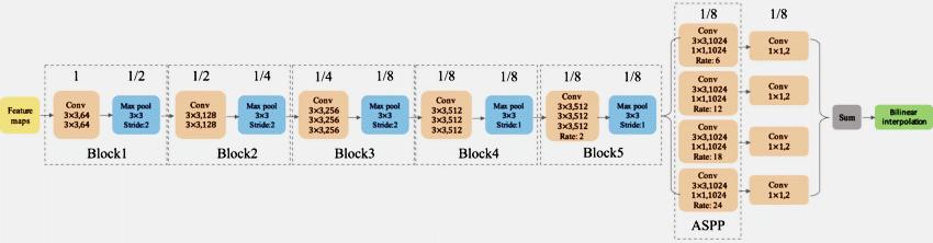
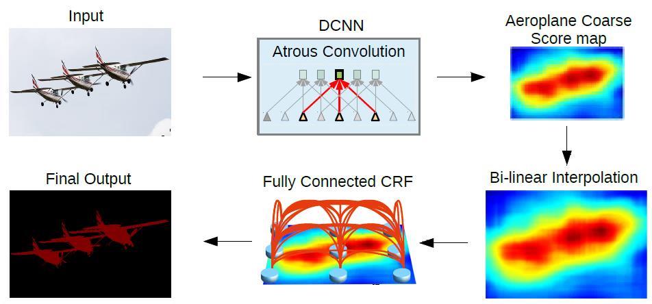
Fig8-b - explain the backbone of deep lab version-2 model.

01- Atrous Convolution:

 It is also called “algorithme à trous” and “hole algorithm”.  It is also called “dilated convolution”.  It is commonly used in wavelet transform and right now it is applied in convolutions for deep learning.

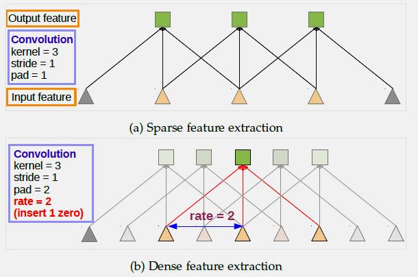
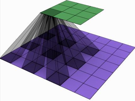
Fig9-a-1 Fig9-a-2

02- Atrous Spatial Pyramid Pooling (ASPP):

 ASPP is an atrous version of SPP, in which the concept has been used in SPPNet.  In ASPP, parallel atrous convolution with different rates are applied in the input feature map, and fuse together.  As objects of the same class can have different scales in the image,  ASPP helps to account for different object scales which can improve the accuracy.

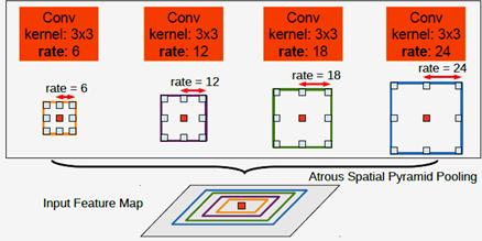
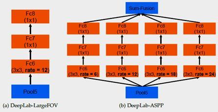
Fig9-b-1 Fig9-b-2

03- Fully Connected Conditional Random Field (CRF):

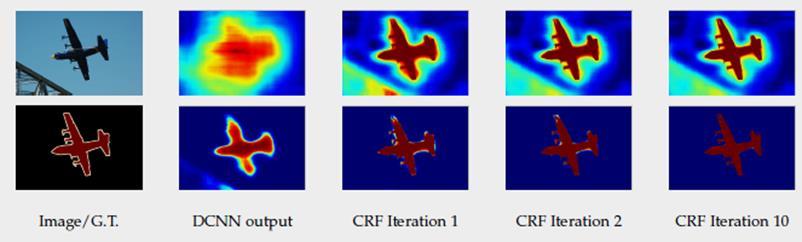
 Fully Connected CRF is applied at the network output after bilinear interpolation.  It is the weighted sum of two kernels:  The first kernel depends on pixel value difference and pixel position difference, which is a Bilateral filter that has the property of preserving edges.  The second kernel only depends on pixel position difference, which is a Gaussian filter.

Adversarial Adaptation to Multiple Targets

As we decided to work with two models Baseline and MTKT, Our first Model `Baseline` strategy is to merge all target datasets into a single one and then deal as a single target. See Figure 11-a.

BASELINE – AdvEnt:  The Segmenter F is decoupled into a Feature Extractor [Ffeat] followed by a Pixel-wise Classifier [Fcls].  Handle ONLY one Source Domain and one Target Domain.  In Multiple Target Domains, we merge all target datasets into a single one  It utilizes an existing single-source single-target UDA framework.

In our second model `MTKT` is a multi-target knowledge transfer, which has a target-specific teacher for each specific target that learns a target-agnostic model thanks to a multiteacher/single-student distillation mechanism. See Figure 11-a.

Multi-Target Knowledge Transfer: Multiple Teachers – Single Student Approach Two types of classifier branches:  Target-specific branches [Multiple Teachers]: each one handles one specific [sourcetarget] domain shift.

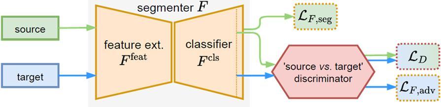
Fig11-a

Fig11-b

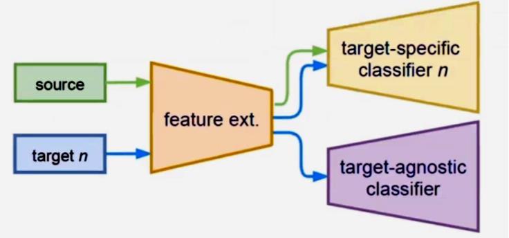
 Target-agnostic branch [One Student]: fuses all the knowledge transferred from the target-specific branches

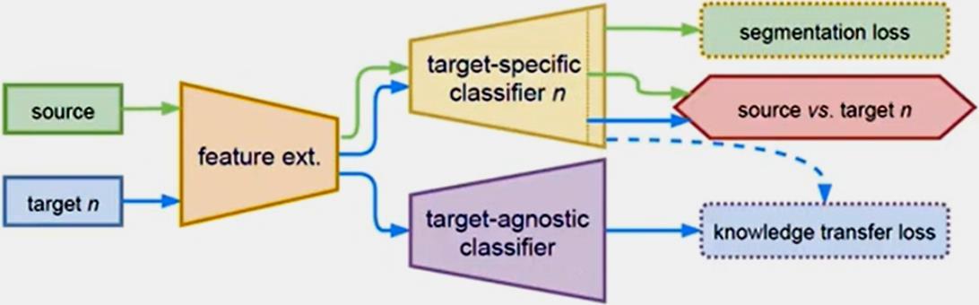
Fig11-b

LOSS FUNCTIONS

#1 Adversarial Discriminator Loss:  The Discriminator [D] is a fully-convolutional binary classifier with parameters (φ).  It classifies the Segmenter’s output (Qx) into either: class 1 (source) or 0 (target).

Targets [Cityscapes + Mapillary]

EQN-1

Fig12-a

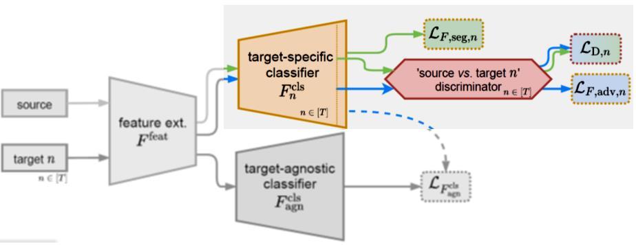
#2 Segmentor Loss:

 The Segmenters [Fcls-n] is trained over its parameters (θ) NOT Only to minimize the supervised segmentation loss LF, seg on sourcedomain data.  But also to fool the discriminator D via minimizing an adversarial loss LF, adv.  The weight [λ_ adv] balancing the two terms.  During training, one alternately minimizes the two losses LD and LF.

2 Target-specific classifiers + 2 Discriminators.

EQN-2

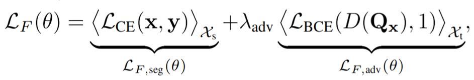
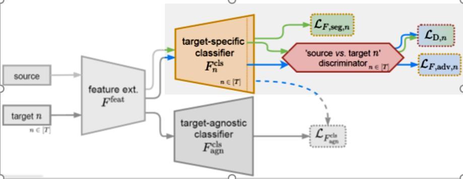
Fig13

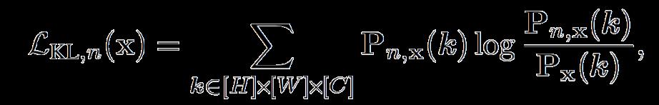
#3 Knowledge Transfer Loss:

 The Agnostic classifier [Fcls-agn] is trained over its parameters to minimize over the segmenter’s parameters (including feature extractors).  The [Student] fuses all the knowledge transferred from the T-targetspecific classifiers [Teachers] via minimizing the Kullback-Leibler divergence between teachers’ and student’s predictions on target domains.

EQN3-a

EQN3-b

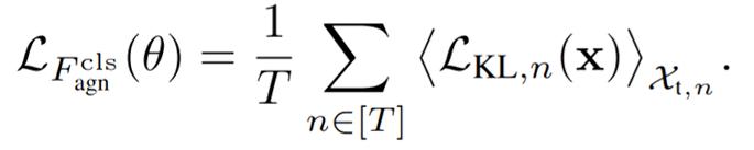
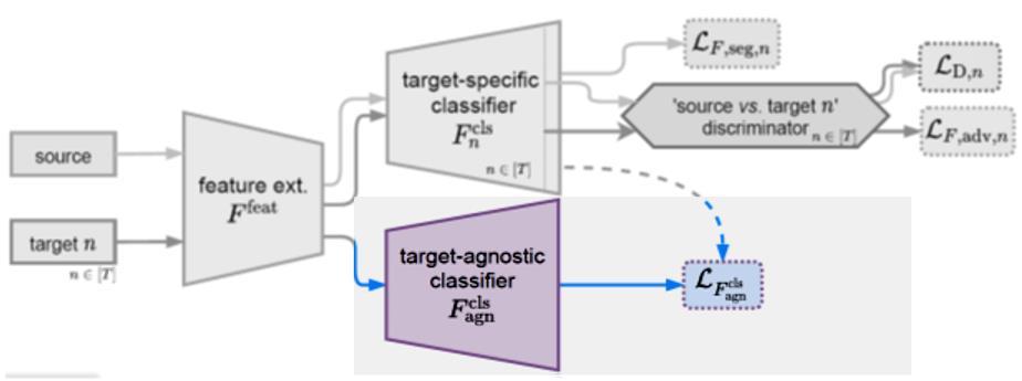
Fig14

Implementation Details

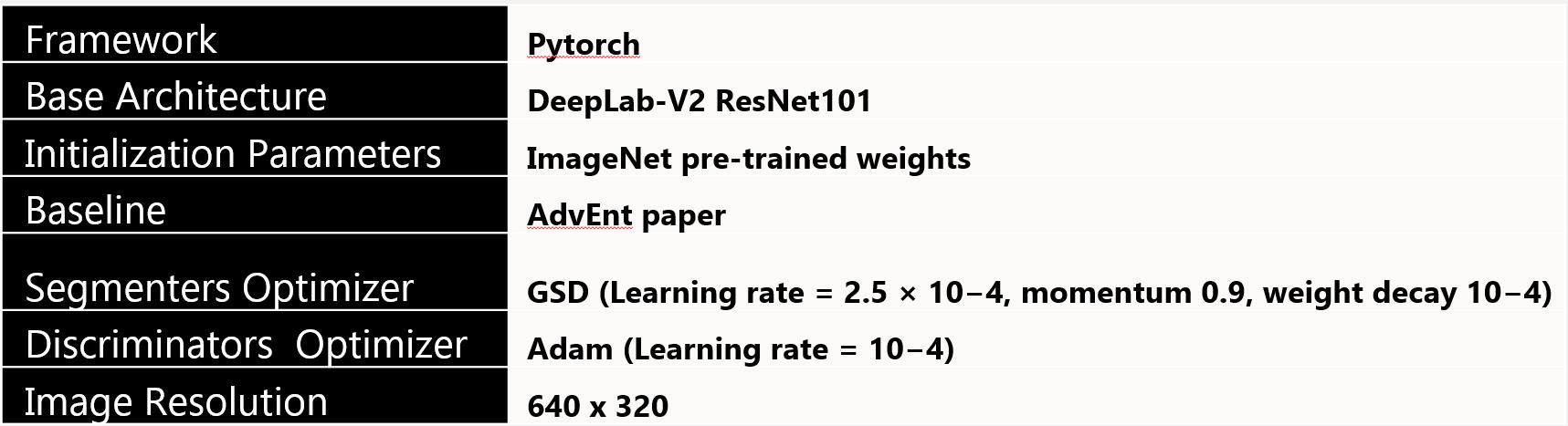
We preferred using Pytorch as our Framework, as we mentioned before we used the pretrained Deep Lab Model version-2,

The below Table shows the implementation details that we used in our experiment:

The important point here is that, the target-specific branches, which is the teacher as the figure 13 explains. We try to learn the feature with 20000 iteration

 In MTKT, we “warm-up” the Target-specific branches for 20,000 iterations before training the Target-agnostic branch.

 The warm-up step avoids the distillation of noisy target predictions in the early phase, which helps stabilize Target-agnostic training.

We introduce two adversarial frameworks: (i) multi-discriminator, which explicitly aligns each target domain to its counterparts, and (ii) multi-target knowledge transfer, which learns a target-agnostic model thanks to a multi-teacher/single-student distillation mechanism. The evaluation is done on four newly-proposed multi-target benchmarks for UDA in semantic segmentation. In all tested scenarios, our approaches consistently outperform baselines, setting competitive standards for the novel task.

Evaluation Metrics - Intersection over Union [ IoU ]

As shown in figure 16-a-2, the IoU is the intersection of predicted and Ground Truth over the union between them.

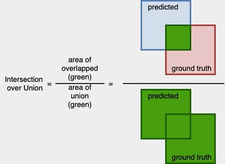
Fig16-a-1 Fig16-a-2

Mapillary

BASELINE

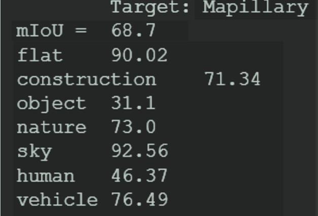
Fig16-b

MTKT

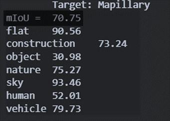
Fig16-d

IoU Score

Cityscapes

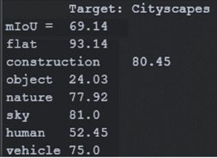
Fig16-c

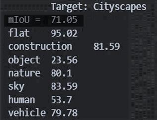
Fig16-e

Features that we care more about