Introduction to 3D Modeling and Parametric Design
Labiba Tasnim

The mathematical research conducted in the late 1970s by mathematician Benoit Mandelbrot gave rise to the field of fractal geometry. Mandelbrot tackled geometric problems in an effort to make them more akin to natural forms. These geometries have the fundamental property that very complex things can be generated by very simple rules. The application of fractal geometry, taking into account the architectural and urban context, enables the production of unlimited iterations that provide room for the examination of the designs' and geometric patterns' efficiency using generative principles. (Arthur Guimarães, 2018)


Since physical time and space have practical bounds, fractal patterns have been modeled extensively, although within a range of scales rather than infinitely. Fractal properties in actual occurrences or theoretical fractals can be simulated via models. The results of the modeling process could be standards for fractal analysis, highly creative depictions, or outputs for further research. There is a list of some particular technological uses for fractals elsewhere. "Fractals" are often used to describe images and other modeling outputs, even when they lack truly fractal features—for example, when zooming in on a portion of the fractal image that shows no fractal attributes.


Nature can generate designs that are less fractal, like crystals. Crystals are neither sufficiently irregular nor sufficiently Euclidian for shapes like straight lines, cubes, triangles, etc. But fractal patterns and self-similarities are commonly seen in crystals (Alexis, 2011).
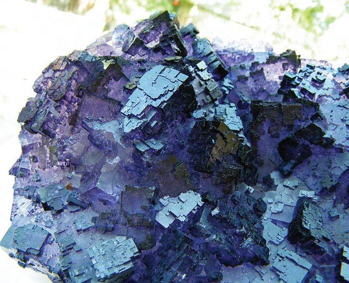
Considering that architecture is a system that has to take complexity into account, new techniques, procedures, and design tools can be produced by applying fractal geometry and crystallization systems to produce complex structures and forms that conventional geometry is completely unable to handle (Arthur Guimarães, 2018)
Steps:

1.Create a triangle and explode

2. Subdivide the edges to construct planes along which initial shapes will be replicated

4. Add boundary surfaces and create a mesh

5. Evaluate the surfaces to construct planes for attractor points

3. Create a basic 3D shape using recursion

6. Start a Anemone Loop to start randomizing the fractal generation

7. End the loop to end randomizing the fractal generation

8. Merge the outputs

9. Apply a gradient to the nal form

Hilbert's curve is among the various "space-filling curves" that occur when a single curve, typically considered a one-dimensional object, "fills" a higher-dimensional space. The two-dimensional region enclosed by a square in this instance is the space filled. The term "space" in the phrase "space-filling" is therefore interpreted in an abstract manner (Richard Kaye. 2017)
Steps:

1.Add a cube and deconstruct it

4.Repeat the pattern

5.Join open ends


2.Extract vertecies and join them accordingly to the a 1 bit per dimentional polyline

3.Rotate, mirror and move the polyline along an axis

In mathematics differential geometry examines the geometry of smooth manifolds, also referred to as smooth shapes and smooth spaces. It makes use of linear algebra, multilinear algebra, differential and integral calculus methods. The field's roots can be found in the ancient study of spherical geometry. It also has connections to astronomy, Earth's geodesy, and later Lobachevsky's research on hyperbolic geometry. The plane and space curves and surfaces in three-dimensional Euclidean space are the most basic examples of smooth spaces, and the study of these shapes served as the foundation for the development of contemporary differential geometry in the eighteenth and nineteenth century.


A triangle immersed in a saddle-shape plane (a hyperbolic paraboloid), as well as two diverging ultraparallel lines.
Differential geometry can be utilized as a technique to comprehend how ideas like the curvature of a plane curve, the angle between two crossing curves, and the distance between two points can be applied to a surface (Mathemetical Institure, 2022).

An isosurface is an isoline's three-dimensional counterpart. It is, in other words, a level set of a continuous function whose domain is 3-space, and it represents points of a constant value (such as pressure, temperature, velocity, or density) within a volume of space. An alternative term for a surface defined by the implicit equation is an isosurface.
F(x,y,z)=f where F is a function of space and f a constant, often 0. The prefix iso- indicates that the function F takes the same value (f) all over the surface (Teraplot, 2013)
Steps:

1.Start with a Brep

4. Point Charge to create magnetic elds

5. Add an IsoSurface component with the created elds


6. Finally merge vertecies


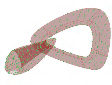
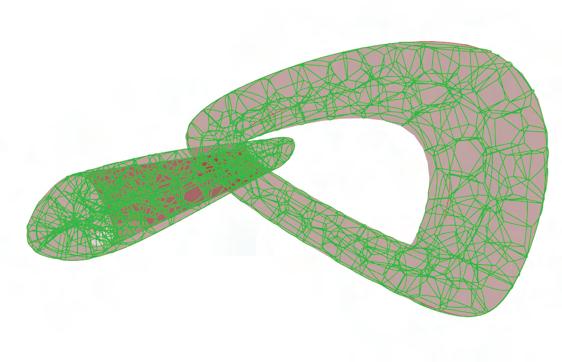
A Möbius strip, also known as a Möbius band or Möbius loop is a minimal surface with zero mean curvature that can be created by joining the ends of a paper strip with a twist. This fascinating mathematical object was first discovered by Johann Benedict Listing and August Ferdinand Möbius in 1858. The Möbius strip is considered a orientable surface, which means that it's impossible to consistently differentiate between clockwise and counterclockwise turns on it. It's interesting to note that every non orientable surface contains a Möbius strip, within its structure (Clifford A., 2005)

1.Start with 2 random 3 dimensional splines

4.Rotate the construction planes


2.Divide the curves into a certain number of segments and join with lines which will act as axix for the strip’s twist

3.Construct planes along the axix where the strip can twist
5.Add a randomizer to the rotation angle to get more dynamic results

6.Finally loft to make a Möbius strip
The artistic design components of biomorphism are based on naturally existing patterns or shapes that are evocative of living things and the natural world. When done to its utmost, it tries to impose organic shapes upon functional tools (HBosler, 2015).


‘growth lounge’, 2016, massif bronze
Biomorphism, also known as bioinspired design or biomimicry, is an innovative approach to design that takes inspiration from nature's forms, processes, and systems to solve human challenges and create more sustainable and efficient solutions. The term "biomorphic" is derived from "bio," meaning life, and "morph," meaning form.

The trefoil knot, known for its threefold symmetry, is a mathematical concept found in nature. Examples include plants with trefoil-like leaf arrangements, molecular structures in biology and chemistry, and certain shells displaying spiral patterns reminiscent of a trefoil.
The trefoil knot can be defined as the curve obtained from the following parametric equations:
x = sin t + 2 sin 2t
y = cos t - 2 cos 2t
z = - sin 3t
import rhinoscriptsyntax as rs import Rhino.Geometry as rg import math
#Define a function to calculate coordinates for the trefoil curve def trefoil_curve(t):
x = math.sin(t) + 2 * math.sin(2 * t)
y = math.cos(t) - 2 * math.cos(2 * t)
z = -math.sin(3 * t)
return rg.Point3d(x, y, z)
#Set parameters if t_values is not None: if isinstance(t_values, (int, float)): t_values = [t_values]
else: t_values = [i * 0.1 for i in range(100)]
#Generate points for the curve points = [trefoil_curve(t) for t in t_values]
#Output pts = points
1.A python script that takes numbers as parameters and gives points in a range for the curve as output


Join the points with the Interpolated curve component

A Voronoi diagram is a structure that divides a plane into areas based on their proximity, to specific points known as seeds. Each area in the diagram includes all the points that're closer to a seed than any other seed in the set. This division of space creates a pattern of polygons on the plane with each polygon representing the area associated with a seed. Voronoi diagrams find applications, in geometry spatial analysis and other fields where understanding relationships and proximity is important.


7. Populate the whole 3D to get seeds8. Cull the duplicate seeds and the ones outside the shapes
10. Use solid intersection to create a single solid object from the volume created all 3D objects intersect

11. Cleaning up duplicate lines

9. Apply

12. Apply Multipipe

13. Apply Laplatian smoothing to get rid of the sharp edges
0, 1, 1, 2, 3, 5, 8, 13, 21, 34, 55, 89, 144, ....
Steps: The Fibonacci sequence is a sequence commonly found in nature, where each number is the sum of the two preceding ones. Numbers that are part of the Fibonacci sequence are known as Fibonacci numbers, commonly denoted Fn . The sequence commonly starts from 0 and 1, although some authors start the sequence from 1 and 1 or sometimes (as did Fibonacci) from 1 and 2. Starting from 0 and 1, the sequence begins:

1.Start with 2 edge circles and divide into parts


2. Divide the height and width into certain number and connect with a spiral of the same number of turns

4. Connect the vertecies of the triangles with Bezier curves of 3 degrees.

3. Connect the edge circles with triangles of increasing height.

5. Add 3 more Bezier curves for each surface using the vertecies of the adjoining triangles as control points
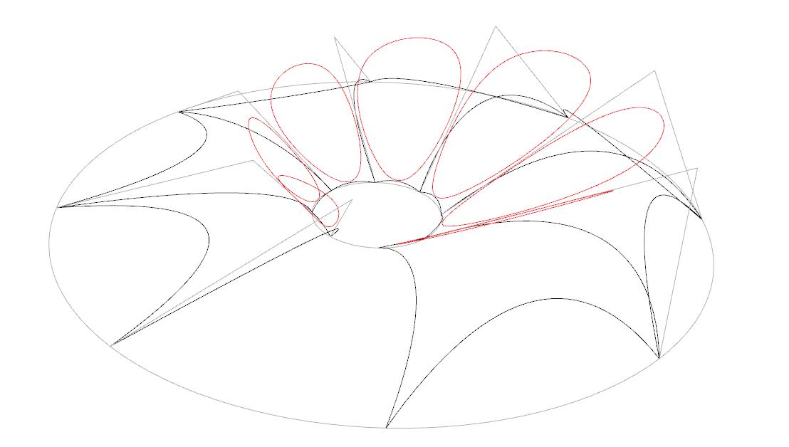
6. Create apartures for all potential surfaces using the vertecies of the guide triangles.

Create surface from the edge curves

8. Use topologicalpy to colorize surface faces according to their increasing height

Topologicpy code:
#Import an obj c = Topology.ByOBJPath(path=r"filepath") Topology.Show(c)
#Get the faces of that obj faces = Topology.Faces(c)
#Iterate through each face using a for loop heights = [] for face in faces:
# For each face get its centroid vertex centroid = Topology.Centroid(face)
#Get the Z of that centroid vertex z = Vertex.Z(centroid) heights.append(z)
#Create a Dictionary with key "z" and value the actual Z value of that centroid d = Dictionary.ByKeyValue('z', z)
#Assign that dictionary to the face dictionary = Topology.SetDictionary(face, d)
#Create list of heights heights = list(set(heights))
#Sort the heights heights.sort()
#Colorize Topology.Show(c, faceGroupKey= 'z', faceGroups=(heights))

9. Applying pipe to the edge curves to gice it structure
An attractor is a collection of states that a system tends to evolve toward in the mathematical subject of dynamical systems, given a wide range of initial circumstances for the system. When system values approach the attractor values sufficiently, they stay there even when there is a small disturbance.
The developing variable in finite-dimensional systems can be algebraically represented as an n-dimensional vector. A region in n-dimensional space is the attractor.

The n dimensions can be two or three positional coordinates for each of one or more physical entities in a physical system; in an economic system, they can be independent variables like the unemployment rate and the inflation rate (Eric W., 2021).
An effect known as "attractor points" occurs when a grid of items varies in shape according to how close it is to one or more specified points. The term "attractor point" refers to the way that the objects in the grid appear to be "attracted" to the point.
This type of effect is very common in computational design since it may provide a complicated effect with a relatively minimal setup. Attractor effects are typically seen as exceptionally lovely and aesthetically pleasing since they are frequently seen in nature (Tait T., 2023).

An effect known as "attractor points" occurs when a grid of items varies in shape according to how close it is to one or more specified points. The term "attractor point" comes from the way the grid's objects appear to be "attracted" to the point (Tait T., 2023).
Steps:

1.Create a series of points

4. Weave the vertecies to create pattern


2. Use the points as centroids for cubes

5. Add an attractor point to maniputale the eld


3. Deconstruct the breps

6. Compute the vector between the attractor point and series of points to orchestrate the series

7. Use the new series of points as centroids for cubes
A curve attractor is a term commonly utilized in the field of geometry and parametric design. It involves employing a curve, such, as a spline or any other type of curved line to govern or influence the behavior of elements within a design.
Setting up an object field, making changes, measuring the distance from the attractor curve, and then adjusting the transformation values based on the distance are the processes required for achieving a curve attractor effect (Tait T., 2023).
Steps:

1.Add a square grid as base

4. Use a circle component that’ll use the grid as base and the curve as eld


2. Add a random curve
3. Extract all the closest points for the curve that will act as the eld

5. Construct domain to set the parameters for the pattern

7. Add a base surface to the pattern 8. Flow the pattern along the 3D surface

6. Use a random 3D surface to wrap the pattern

Finally delete input 3D surface
DataGenetics, 2013 Hilbert’s Curve. [Online] Available at: http://datagenetics.com/blog/march22013/index.htm
Fractal Forums, 2021. Fractal Crystal. [Online] Available at: https://www.fractalforums.com/fractals -in-nature/fractal-crystal/
Guimarães, Year. Fractal Theory, Crystal Formation Process, and Its Architectural Implications: Case Study on the Process of Prototyping Complex Forms. [Online] Available at: https://www.linkedin.com/pulse/fractal -theory-crystal-formation-process-its-case-studyguimar%C3%A3es/
Howard Bosler, 2015 Mid Century Modern Groovy. [Online] Available at: https://www.midcenturymoderngroovy.com/?p=1523
Kaye, R.W., 2017 Hilbert’s Curve. [Online] Available at: http://web.mat.bham.ac.uk/R.W.Kaye/
Pickover, C. A. (2005). The Möbius Strip: Dr. August Möbius's Marvelous Band in Mathematics, Games, Literature, Art, Technology, and Cosmology. Thunder's Mouth Press, pp. 28–29. ISBN 978-1-56025-826-1.
Shengmorni, 1963. [Online] Available at: https://medium.com/@shengmorni/196388a359d2f68b
Thomas Tait, 2023. Attractor Curve in Grasshopper. [Online] Available at: https://hopific.com/attractor-curve-in-grasshopper
Weisstein, E. W. (2021). Attractor. MathWorld. [Online] Available at: https://mathworld.wolfram.com/Attractor.html
MSc Computational Methods in Architecture 23-24
Cardiff University