Atmospheric CO2: Exploring the Role of Sea Surface Temperatures by John A. Shanahan

Atmospheric CO2:ExploringtheRoleofSeaSurface TemperaturesandtheInfluenceofAnthropogenicCO2

Bernard Robbins - Independent Researcher Manchester,UK

Abstract

Close examination of the small perturbations within the atmospheric CO2 trend, as measured at MaunaLoa,revealsastrongcorrelationwithvariationsinseasurfacetemperatures(SSTs),most notably with those in the tropics. The temperature-dependent process of CO2 degassing and absorptionviaseasurfacesiswell-documented,andchangesinSSTswillalsocoincidewithchanges in terrestrial temperatures, and temperature-dependent changes in the marine and terrestrial biospheres with their associated carbon cycles. Using SST and Mauna Loa datasets, three methods of analysis are presented that seek to identify and estimate the anthropogenic and, by default, naturalcomponentsofrecentincreasesinatmosphericCO2,anassumptionbeingthatchangesin SSTs coincide with changes in nature’s influence, as a whole, on atmospheric CO2 levels. The findings of the analyses suggest that an anthropogenic component is likely to be less than 10 % of the increase sincethe mid-1990s, withfigures of uptoaround 6% being estimatedfromdata acquiredsince1995.Theinferenceisthatmorethan90%ofthoseincreasesareofnaturalorigin, andindeedthefindingssuggestthatnatureiscontinuallyworkingtomaintainanatmospheric/surfaceCO2 balance,whichisitselfdependentontemperature.Afurtherpointertothisbalancemay come from chemical measurements that indicate a brief peak in atmospheric CO2 levels centred aroundthe1940s,andthatcoincidedwithapeakinglobalSSTs.

Keywords:AtmosphericCO2;SeaSurfaceTemperatures;AnthropogenicCO2

Submitted2024-03-16,Accepted2025-07-03.https://doi.org/10.53234/scc202504/23

1.Introduction

Research into the influence SSTs have on changes in atmospheric CO2 includes the work by Humlum et al. (2013). When examining phase relationships, they found a maximum correlation forchangesinatmosphericCO2 lagging11-12monthsbehindthoseofglobalSSTs[1]. Apaper bythelateFredGoldberg(2008)notedtheircorrelationbyexaminingElNiñoevents[2].Healso consideredHenry’slaw[3]inrelationtoSSTs,i.e.atemperature-dependentequilibriumbetween atmospheric CO2 and its solubility in seawater. Spencer (2008) also noted similarities between surfacetemperaturevariationswithchangesinatmosphericCO2 [4].

For the oceans specifically, areas of surface CO2 absorption and degassing are shown in maps provided by NOAA [5] and ESA [6] for example. These maps show that colder sea surfaces towards the poles are net absorbers of CO2 whilst the warmer surface waters of thetropics are net emitters.AnanalogyoftencitedisthegreaterabilityofcarbonateddrinkstoretainCO2 atcooler temperatures;thisabilitydropsasthedrinksgetwarmer.

AstrongcorrelationbetweenchangesinatmosphericCO2 andSSTscanbereadilydiscernedfrom the relevant datasets. To illustrate, the upper graph in Fig. 1 plots atmospheric CO2 in parts per million(ppm) asmeasuredatMauna Loa, Hawaii, since 1982.The data [7] has been ‘deseasonalised’byNOAAtoremovenaturalannualCO2 cycles.

https://scienceofclimatechange.org

Bernard Robbins: Sea Surface Temperatures and Recent Increases in Atmospheric CO2

DeseasonalisedAtmosphericCO2ppm-MaunaLoa andMonthlyAveragedCO2ppmIncrease(12-MonthAverage-AverageofPreviousMonth)

Figure 1: Deseasonalised atmospheric CO2 data (Mauna Loa).

Itcanbeseenthatthegraph’sgeneraltrendexhibitssmallperturbations.Thesecanbemagnified by plotting the monthly CO2 ppm increases with time, and the lower graph in the figure shows averaged monthly ppm increases over the same time period. Averaging removes some of the ‘noise’ from the trace.Distinct peaks and troughs are now apparent in the data. If global tropic SSTs[8]areoverlaidontothelowergraph,astrongcorrelationisobserved,Fig.2.

TropicSSTAnomalyandAveragedMonthlyMaunaLoaCO2ppmIncrease (12-MonthAverage-AverageofPreviousMonth)

Figure 2: Global tropic SSTs overlaid onto monthly atmospheric CO2 increases (Mauna Loa)

The similarity between the two traces is striking: short-term fluctuations in CO2 readings at Mauna Loa appear particularly sensitive to tropic conditions (if tropic SSTs are substituted for global SSTs in Fig. 2, the correlation is less strong). Warm tropical seas, with surface temperaturestypicallyaround25-30 oC,coveralmostonethirdoftheearth’ssurface.Themostprominent peaks in the figure coincide with strong El Niño events. Taken at face value, and ignoring any influencefrom anthropogenicemissions, Fig. 2suggeststhatifthetropic SST anomaly dropped toaround-1 oC(withrelateddropsglobally)thentheconcentrationofCO2 intheatmosphere,as measuredatMaunaLoa,wouldleveloff.

An important point is that changes in SSTs will coincide with those of terrestrial temperatures, temperature-dependentchangestobothterrestrialandmarinecarboncyclesand,takingintoconsideration the research by Humlum et al. (2013) who found that changes in atmospheric CO2 followedchangesinSSTs,anassumptionintheworkpresentedhereisthatnature’sinfluenceon atmosphericCO2 levels,asawhole,followsonfromchangesinSSTs.

https://scienceofclimatechange.org

Thebasisbehindsuchanassumptionisexaminedinmoredetailasfollows:

In a 2022 article, Schrijver [9] summarises his interpretation of recent events regarding atmospheric CO2, writing:“The...increaseintheaverageglobaltemperaturehasresultedinahigher annualnaturalemissionsfromlandandsea…Theincreaseinbothnaturalandanthropogenic emissionshasledtomoreCO₂intheatmosphere...Thehigherconcentrationresultsinagreater down-fluxtobothseaandland...Theincreaseinconcentrationintheatmosphereistheresultof acombinationofincreasedtemperatureandhumanemissions.”

Fortheoceans,andconsideringHenry’slaw,SchrijverdescribeshowbothatmosphericCO2 concentrations and water temperature influences the exchange of CO2 at the sea surface: higher atmosphericconcentrationsresult inanincreasedCO2 absorption,whereasa higherwatertemperature results in reduced CO2 retention. The implication is that some ‘re-balancing’ of seawater CO2 concentrationstakesplace.

For the land, Schrijver says: “AbouthalfoftheCO₂thatplantsabsorbthroughphotosynthesis disappearsalmostimmediatelyintotheatmosphereintheformofplantrespiration.Theother halfisconvertedintobiomass(leaves,wood,roots,etc.)thatendsuponorintheground.” He alsodiscussesthetemperature-dependencyofsoilrespiration.Onthissubject,Harde(2023)[10] concluded: “Particularlysoilrespirationinthetropicsandmid-latitudescanbeidentifiedasthe mainnaturalsourceofCO2 emissions.”

Regarding the significance of the tropics in relation to atmospheric CO2 increases, Harde and Salby (2021) [11] say in their abstract:“Thermally-inducedemission, especiallyfromtropical landsurface,isfoundtorepresentmuchoftheobservedevolutionofnetCO2 emission” andthey conclude:“NetemissionofCO2,whichistheresultant ofallcontributions,isconcentratedat tropicallatitudes”.

It might be suggested that it is increases in anthropogenic CO2 thatare driving SSTs in Fig. 2. However,bywayofexample,referringtotheprominent1998peakinthefigure,theCO2 increase in 1998 was three times that in 1999. If this was a result of human emissions then these would have been three times as much in 1998 as ‘99. Data supplied by the GCB website [12] suggest thesewereabout24.9Gtin1998and25.4Gtin1999:verysimilar.The1998CO2 peaktherefore points to a natural origin and corresponds to a strong El Niño event with its associated warmer SSTs.

2.MaterialsandMethods

The observations described above serve as a starting point for the data analyses presented here, whichfirstseektoidentifyandestimateananthropogenicCO2 signaturefromwithinthisapparent natural atmospheric CO2/SST relationship. Microsoft® Excel® is used throughout for data processing,graphics(exceptFig.9),linearregressiontrendlinesandcurve-fitting.

2.1Analysis1:UsingaShortTimeWindow

Using the data presented in Fig. 2, the first analysis method uses the relationship between the prominentshort-termfluctuationinSSTsatthetimeofthe1998ElNiñoevent,andatmospheric CO2 increases over the same time period,to try to discern, and roughly-quantify, a human component within the CO2 trend of the last few decades. Data prior to 1995 is excluded due to the 1982 El Chichon & 1992 Mt. Pinatubo volcanic eruptions that served to suppress atmospheric CO2 levels. GCB data [12] suggests roughly half of all anthropogenic CO2 emissions have occurredsince1995withannualemissionsincreasingbyabout60%sincethen.

Theanalysisprocedureisasfollows:

Using only the data from within the green inset box, Fig. 3, the time of the 1998 El Niño event, establish the relationship between monthly CO2 ppm increase and SST anomaly, Fig. 4. This eventincorporatesabroadrangeofSSTvalueswhichhelpsoptimisetheaccuracyoftheanalysis. Theevent’sshorttimeframe(~2.5years)meansthatthisrelationshipis,essentially,independent

https://scienceofclimatechange.org

Bernard Robbins: Sea Surface Temperatures and Recent Increases in Atmospheric CO2

ofanylonger-termppmincreaseresultingfromtheriseinhumanemissions.

NowapplytherelationshipderivedinFig.4tothewholeSSTdatasetofFig.3i.e.calculatefrom each monthly SST value the CO2 ppm increase for every month starting in 1995. Then sum all thesemonthlyincreasestoproduceacalculatedtotalvalue(CTV)ofppmincrease.

ThemeasuredCO2 increasesince1995was62ppm(Fig.1).IftheCTVislessthanthismeasured increase, then this could suggest the difference is a possible human component. For example, if the CTV is 52 ppm, then the 10 ppm difference might be attributed to the increase in human emissions of CO2 since the mid-1990s. If the CTV is about the same as the measured increase, thenthispointstoanon-discerniblehumancomponentofCO2

TropicSSTAnomalyandMaunaLoaCO2ppmIncrease (12-MonthAverage-AverageofPreviousMonth)

DATAUSEDTO ESTABLISHSST/CO2 RELATIONSHIP

ppmIncrease

Figure 3: The 1998 El Niño data ‘Window’ (Green Inset Box) used to establish the CO2/SST data relationship shown in Fig. 4.

SSTAnomaly(Deg.C)

Figure 4: Using only the data from within Fig. 3’s inset box, values of SST and monthly CO2 increase with the same time stamp are plotted as x-y values, together with a fitted linear trend line and associated equation. This equation (y = the monthly CO2 ppm increase as a function of SST (x)) is then applied to every month of the whole SST dataset (1995 onwards) to calculate the final CTV.

Fig. 5 now plots cumulative monthly CO2 increases calculated from the SST data using Fig. 4’s equation,startingat360ppmandendingat(360+CTV)ppm.Measuredvaluesarealsoshown.

https://scienceofclimatechange.org

1998ElNino

MeasuredCO2ppm(MaunaLoa)andCalculatedValuesderivedfromTropicSSTData (1998ElNinoppmIncreasevsSSTRelationshipEmployedforCalculations)

Valuesaligned atstartofdata.

ValuesCalculatedfromSSTs

Figure 5: Calculated monthly CO2 ppm values since 1995, based on SSTs, and Mauna Loa values. The final CTV and measured increase are both 62 ppm i.e. a human component is not discernible.

2.2 Analysis 2: Using a Moving SST Window

With the same aim as Analysis 1, this method uses the same data sets. Again, the years prior to 1995havebeenexcludedtoavoidpossiblebiasingoftheresultsduetothe1982&1992volcanic eruptions. Thismethodtakes‘slices’throughthedataatdifferentSSTs,Fig.6.

TropicSSTAnomalyandAveragedMonthlyMaunaLoaCO2ppmIncrease (12-MonthAverage-AverageofPreviousMonth)

Figure 6: A typical ‘Slice’ or ‘Window’ for a 0.2 oC range of SSTs (1995 onwards)

This methodanalysesSSTdatathatis onlywithinthe chosen‘slice’or‘window’.MonthlyCO2 increases,withthesametimestampastheSSTdata,areplottedasafunctionoftime.Anassumption when using this method is that, if there is no influence from anthropogenic emissions, then there should be no upward trend in these increases as time progresses. However, if increasing annualanthropogenicemissionsarecontributingtothoseincreases(GCBdatasuggeststheyhave increasedbyabout60%since1995),thenthismayshowupintheresultingtrends.

Fig.7fshowsthetrendinmonthlyppmincreasesfromthewindowidentifiedinFig.6.Thefitted trendlineshowsaveryslightpositivegradientresultinginachangeinmonthlyincreaseof0.0084 ppm since 1995, as calculated from the trend line’s gradient. This exercise is performed as the windowmovesbetween-0.3and0.6 oCinstepsof0.1 oC,resultinginthetrendlines,withequations, in Figs. 7(a-h). The highest and lowest SSTs are excluded from the analysis due to there beinginsufficientdatapoints.

Bernard Robbins: Sea Surface Temperatures and Recent Increases in Atmospheric CO2

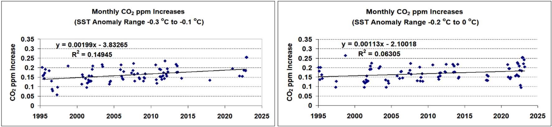
7 (a & b): Monthly CO2 ppm increases for SST anomaly windows -0.3 to -0.1 & -0.2 to 0 oC.

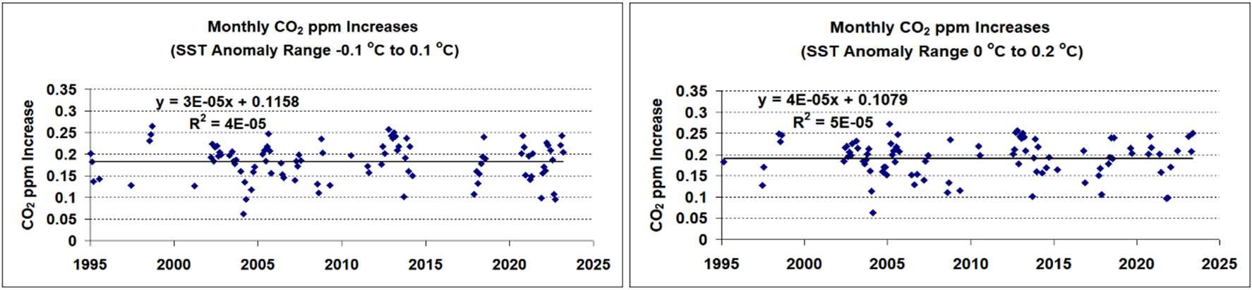
7 (c & d): Monthly CO2 ppm increases for SST anomaly windows

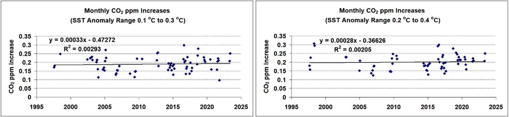
7 (e & f):

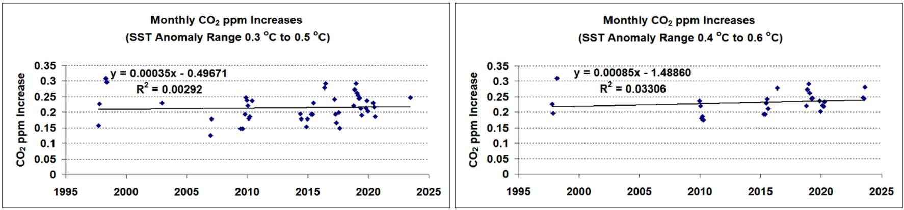
7 (g & h): Monthly CO2 ppm increases for SST anomaly windows -0.3 to 0.5 & 0.4 to 0.6 oC.

Theaveragetrendlinegradientfromall eight‘windows’or‘slices’is+0.000625ppmchangein the monthly increase, per year. At the end of the ~28-year period this equates to a change of +0.0175ppm/month(thisfigurecanbeapproximatelyderivedbyvisuallyexaminingthechange in trend line end point values for each graph, and then averaging). Assuming that this change could be attributed to anthropogenic emissions, an estimate can be made of the percentage contributionoftheseemissionstothetotalatmosphericCO2 increaseasfollows:

Assuming a linear increase in annual anthropogenic emissions since 1995 (see Fig. 8) calculate the change in ppm increase for each month, based on the 0.0175 ppm end-point figure. So, for example, the monthly change halfway through the period would be half of that value. Then for all336monthsoverthe28-yearperiod,sumeachincrementalmonthlychangewithrespecttothe startof1995,startingat0ppmandendingat0.0175ppm,asillustratedinFig.9.Thecumulative sumofall336incrementalchangesinmonthlyppmincreasescomestoalmost3ppm.

Figure

Figure 8: Annual anthropogenic CO2 emissions (GCB data – Blue Trace). A linear rise in emissions (Grey Line) is assumed for the final summed calculation (Fig. 9)

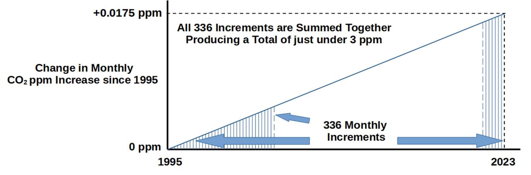
Figure 9: Assuming a linear rise in annual anthropogenic emissions from 1995 (see Fig. 8), the cumulative sum of all 336 incremental changes in monthly ppm increases comes to almost 3 ppm.

3.Results(Analyses1&2)

For Analysis 1, the calculated CO2 ppm increase (from SSTs) and the measured increase, since 1995,areincloseagreementatabout62ppmi.e.ahumancontributioncannotbediscerned.

For Analysis 2, the cumulative sum of all 336 incremental changes in monthly ppm increases comes to almost 3 ppm. Mauna Loa data suggests the total atmospheric CO2 ppm increase over thisperiodisabout 62ppm.Thus,the calculationsusingthisanalysismethodsuggesta possible humancontributionof3ppmoutof62ppm,orabout5%overthe28-yearperiod.

It might be argued that the‘large’ 0.2 oC window used in Analysis 2 may inadvertently bias the trendlinegradients inamorepositive direction,duetoa netincreaseinSSTvalues(andassociatedppmincreases)withinthewindow,astimeprogresses.Ifso,thiswouldexaggerateanypossible humancontribution.To minimise any bias,if itexists,the aboveexercisewas repeatedfor seventhinner0.1 oC‘slices’orwindowsinstepsof0.1 oCovertheSSTanomalyrangeof-0.2to 0.4 oC. This repeated exercise suggested a possible human contribution of just under 4 ppm out of 62ppm,orabout6%.Goingtothinnerwindowsstillisnotpractical,duetherebeingtoofew datapointsineachwindow.

The two analysis methods just described produce approximate results and so are useful for estimation only. Broadly-speaking, they suggest a quantifiable atmospheric CO2 increase, possibly attributedtohumanemissions,oflessthan10%,andperhapscloserto5%,ofthetotal overthe lastthreedecades,thusinferringthatmorethan90%isofnaturalorigin.

4.Analysis3:Longer-TermDataTrends

UsingabroadlysimilartechniquetothatdescribedbythelateLanceEndersbee(2008)[13],this thirdanalysismethodplotsatmosphericCO2 againstlonger-termtrendsinSSTs.

To do this, the spreadsheet software applies a second degree polynomial curve fit to tropic and globalSSTdatasets,essentiallyactingasalow-passfilterthatsmoothsoutthepeaksandtroughs thatareprincipallyaconsequenceofElNiñoandLaNiñaevents.

4.1 3a. Global Tropic SSTs since 1982

Fig.10showsaseconddegreepolynomialcurvefittotheglobaltropicSSTdataofFig.2together withtheassociatedequation.

TropicSSTAnomalyandAveragedMonthlyMaunaLoaCO2ppmIncrease (12-MonthAverage-AverageofPreviousMonth)

SSTAnomaly ppmIncrease

VOLCANICERUPTIONS: ELCHICHON1982MT.PINATUBO1992

y=1.922905E-04x2-7.559966E-01x+7.427098E+02

Figure 10: Polynomial curve fit to global tropic SSTs since 1982

The equation forthis curve fit is then usedto plot the trend of atmospheric CO2 asa function of the ‘smoothed’ tropic SST data, both parameters possessing the same timestamp for each data point,Fig.11.Afittedlinear trendline (withassociatedequation)is superimposed.Date stamps areshownatselectedCO2 ppmlevels.

CO2ppm(MaunaLoa)versusTropicSSTAnomalybasedon1982-2023NOAAData. SSTAnomaliesCalculatedfromaSecondDegreePolynomialCurveFittotheRawData

y=133.32x+384.19 (or133ppm/deg.C)

-0.4-0.3-0.2-0.100.10.20.30.4

Figure 11: Atmospheric CO2 as a function of the global tropic SST trend since 1982

Bernard Robbins: Sea Surface Temperatures and Recent Increases in Atmospheric CO2

4.23b.EastPacificTropicSSTs (81W-179W,27S-27N)Since1951

This data[14]goesbackto1950.Again,thespreadsheetsoftwareappliesa seconddegree polynomialcurve fit tothe data,Fig.12.Notethatthe SSTanomaliesforthisdatasetare assumedto be in degrees Fahrenheit, and not Celsius as was stated on the website that the data was downloadedfrom.

EastPacificTropicSSTs(81W-179W,27S-27N)Since1951(NOAAData) withSecondDegreePolynomialCurveFit

SST Anomaly (Deg. F Assumed)

y=0.000186025x2-0.715938547x+687.612336808

Figure 12: East Pacific tropic SSTs since 1950 (degrees Fahrenheit assumed)

TheSSTanomalyisthedifferencefromachosenbaseline,orzeroreferencepoint.Thisreference pointisnormallyameanSSTvalueaveragedbetweentwoearlierdates.

Using the data from the smoothed SST curve fit, above, the resulting trend of atmospheric CO2 asafunctionofSSTisshowninFig.13,togetherwithfittedlineartrendlineandequation.

CO2ppm(MaunaLoa)versusEastPacificTropicSSTAnomaly(81W-179W,27S-27N) Basedon1959-2023NOAAData SSTAnomalies(Deg.FAssumed)fromSecondDegreePolynomialCurveFitofRawData

y=66.225x+381.62 (66ppm/deg.For119ppm/deg.C)

-1.2-1-0.8-0.6-0.4-0.200.20.40.60.8 SSTAnomaly(Deg.FAssumed)

Figure 13: Atmospheric CO2 as a function of East Pacific Tropic SST trend since 1958. As a point of reference, GCB data suggests more than 80 % of human CO2 emissions have occurredsince1958

https://scienceofclimatechange.org

Bernard Robbins: Sea Surface Temperatures and Recent Increases in Atmospheric CO2

4.3 3c. Global SSTs Since 1958

TheexerciseisrepeatedhereusingglobalSSTdata[15]ascomparedtotropicSSTdata.Asecond degreepolynomialcurveisonceagainfittedusingthespreadsheetsoftware,producingtheequationshowninFig.14.

GlobalSeaSurfaceTemperaturesSince1958(NOAAData) withSecondDegreePolynomialCurveFit

SST Anomaly (Deg. C)

y=7.25682E-05x2-2.77641E-01x+2.65409E+02

GLOBAL19551965197519851995200520152025

Figure 14: Global SSTs since 1958

Using the data from the smoothed SST curve fit, above, the resulting trend of atmospheric CO2 asafunctionofglobalSSTisshowninFig.15,togetherwithfittedlineartrendlineandassociated equation.

CO2ppm(MaunaLoa)versusGlobalSSTAnomalybasedon1959-2023NOAAData. SSTAnomaliesfromSecondDegreePolynomialCurveFitofRawData

y=144x+312.72 or144ppm/deg.C

GlobalSSTAnomaly(Deg.C)

Figure 15: Atmospheric CO2 as a function of global SST trend since 1958

5.Results(Analysis3)

ApproximatelineartrendsareapparentforallthreegraphsinFigs.11,13and15,withfittedtrend linegradientsof:

 133ppm/ 0CforglobaltropicSSTssince1982.

 119ppm/ 0CforEastPacifictropicSSTssince1958(it’sinterestingtonotethatthetrend linealmosthidesthegraphduetothegraph’slinearity).

 144ppm/ 0CforglobalSSTssince1958.

https://scienceofclimatechange.org

6.Discussion

The techniques used in Analyses 1 and 2, aimed at discerning and estimating the human contributiontorecentincreasesinatmosphericCO2,arebasedonprocessingofmonthlydatafromboth SSTandatmosphericCO2 datasets.

UsingthetechniquedescribedinAnalysis1,nocontributionfromhumanemissionstothemeasured increases in atmospheric CO2, since 1995, was discerned. For the technique described in Analysis2,figuresofaround3and4ppmwerecalculatedforapossiblehumancontributionout ofatotalincreaseof62ppmsince1995,equatingtoaround5%and6%,respectively,ofthetotal increaseinatmosphericCO2 since1995.

Thus,theresultsofthesetwoanalyses,takentogether,suggestthatnatureaccountsformorethan 90%,perhapsnearer95%,ofincreasesinatmosphericCO2 since1995.

The technique described in Analysis 3 examines the relationship between longer-term trends in SSTdatasetsandatmospheric CO2 measurements. Thisdataanalysisgoesasfar backasthelate 1950s, when the ongoing acquisition of atmospheric CO2 measurements began at Mauna Loa. The resulting three graphs show an apparent almost-linear long-term relationship between SSTs andatmosphericCO2.Lineartrendlinesfittedtothesegraphsproducegradientsofbetween~120 and~145ppm/ 0CforthethreeSSTdatasetsexamined.

AsforanthropogenicCO2,publishedfigures(e.g.GCBdata)suggestaroughlylinearrelationship between cumulative anthropogenic emissions as a function of time, and atmospheric CO2 measurements from Mauna Loa.If it’s reasonedthat thismostly accounts for thelinear trendsas calculatedinAnalysis3,thisreasoningwouldnotfitwiththefindingsofthefirsttwoanalysismethodsthatsuggestthatmorethan90%ofrecentatmosphericCO2 increasesareofnaturalorigin.

6.1 Comparison with Other Recent Publications

AnumberofrecentpapersandarticlesputforwardacaseforrecentincreasesinatmosphericCO2 being mostly natural. Conclusions are drawn from several different lines of reasoning, and the approaches used are different to those presented above. Here are some examples (excerpts are fromabstractsunlessotherwisestated):

Humlum at al. (2013) [1] based on analysis of several well-known datasets (this excerpt is from theirSection8): “Summingup,ouranalysissuggeststhatchangesinatmosphericCO2 appearto occurlargelyindependentlyofchangesinanthropogenicemissions... bythiswehavenotdemonstratedthatCO2 releasedbyburningfossilfuelsiswithoutinfluenceontheamountofatmospheric CO2,butmerelythattheeffectissmallcomparedtotheeffectofotherprocesses.”

Skrableetal.(2022)[16]byexamining14C: “Wedeterminedthatin2018,atmosphericanthropogenicfossilCO2 represented23%ofthetotalemissionssince1750…”

Schroder (2022) [17]: “Overtheindustrialera,thenaturalemissionincreasedthreetimesas muchastheman-made.Theresultisthatonlyabout25percentoftheincreaseinatmospheric CO2 isman-made”

Salby & Harde (2022) [18]conclude: “Thermally-inducedemissioninthetropicscloselytracks observednetemissionofCO2.ItthusaccountsforthepreponderanceofCO2 netemission,which inturndeterminesanomalousCO2.Forthisreason,thethermally-inducedresponsetoobserved warminginthetropicsrepresentsnearlyalloftheobservedincreaseofatmosphericCO2.”

Berry (2023) [19]: “UNdatashowhumancarbonemissionshaveaddedonly33ppmtoatmosphericCO2...Thispredictedhuman-causedincreaseof33ppmis8%ofthetotalcarboninthe atmosphereasof2020…Also,δ14CdataprovenatureistheoverwhelmingcauseoftheCO2 increasesince1750,andlowerthe8%ofhumancarbonintheatmospherecalculatedfromthe UNdatatolessthan4percent.”

Bernard Robbins: Sea Surface Temperatures and Recent Increases in Atmospheric CO2

Harde (2023) [20]: “WepresentowncalculationsbasedontheConservationLaw,whichreproducealldetailsofthemeasuredatmosphericCO2 concentrationovertheMaunaLoaEra.From thecalculationswederiveananthropogeniccontributiontotheobservedincreaseofCO2 over theIndustrialEraofonly15%.”

Koutsoyiannis (2024) [21]: “Examining isotopic data in four important observation sites, we showthatthestandardmetricδ13Cisconsistentwithaninputisotopicsignaturethatisstable overtheentireperiodofobservations(>40years),i.e.notaffectedbyincreasesinhumanCO2 emissions.Inaddition,proxydatacoveringtheperiodafter1500ADalsoshowstablebehaviour. Thesefindingsconfirmthemajorroleofthebiosphereinthecarboncycleandanon-discernible signatureofhumans.”

Ato(2024)[22]: “thisstudyisthefirsttousemultipleregressionanalysistodemonstratethatthe independentdeterminantoftheannualincreaseinatmosphericCO₂concentrationwasSST” and concludes: “TheglobalSSThasbeenthemaindeterminantofannualincreasesinatmospheric CO₂concentrationssince1959.Nohumanimpactwasobserved.”

Shelley(2024)[23]saysinarecenton-linearticle: “...Iproposethattheobservedoceanwarming since1905…hasresultedinthereleaseofoceanicCO2,whichisthemainreasonwhyatmosphericCO2 hasincreasedby140ppm.”

Schrijver (2024) [24] concludes: “Duetothedominantroleofnaturalchangesinthebiosphere undertheinfluenceofhighertemperatures,onecanconcludethatthepresentCO₂concentration canberegardedasa‘natural’level.”...“Withasingleresidencetimeforallcarbondioxidein theatmospherethehumancontributionbasedonfossilfuelsisapproximately4.3%…”

SummarisingtheabovefiguresforhumancontributionstoatmosphericCO2 sincethestartofthe industrialrevolution,theseare:25%(Schroder),23%to2018(Skrableetal.),15%(Harde),13 %*(Schrijver)and<12%*(Berry)(*estimatedfrom%oftotalatmosphericCO2).Both Atoand Koutsoyiannissuggestnodiscerniblehumancontribution.

Bycomparison,themaximumestimatedfigurefromtheanalysesinthispaperis~6%since1995, and GCB data suggests that roughly half of total human emissions have occurred since 1995. Simple extrapolation of the 6 % figure back to the start of the industrial revolution is therefore roughly double at ~12 %. This simple extrapolation should be viewed with a little caution, but may be useful as a comparison to the above figures, falling roughly midway between the 25 % figureandnodiscerniblehumancontribution.

Withregardstotheppm/ oCtrendlinegradientsderivedinAnalysis3ofthispaper, thesegradients(averaging~130ppm/ oC)arebroadly-similartothegradientofthegraphinFig.3ofHarde’s 2017paper[25],forsurfacetemperaturesofthelastfiftyyearsorso.

ReferringagaintothefindingsofAnalyses1-3inthispaper,factorsthatmayexplainthesefindings are now considered (note that the majority of these factors are discussed by the aforementionedauthors).

6.2 A Natural CO2 Surface/Atmosphere Balance?

The idea of a natural CO2 surface/atmosphere balance is nothing new. In his 2008 paper, Goldberg, for example, considered Henry’s law as a fundamental contributor to such a balance. This states that the amount of gas dissolved in a liquid is directly proportional to the gas’s partial pressure above the liquid. The law applies to any water exposed to the atmosphere, from ocean surfaces to cloud droplets, and the associated temperature-dependency means that cold water is abletoretainmoreCO2 thanwarmwater.

Whenconsideringtheoceans,mostoftheabsorbedCO2 undergoeschemicaldissociation,orionisation:the vastmajorityseemingly‘prefers’totakethe formof bicarbonateandcarbonateions. WhenCO2 isreleasedfromtheoceans,thechemistryworksinthereversedirection.Henry’slaw

https://scienceofclimatechange.org

applies to CO2 as a gas only, not to its associated ionic species, and simple calculations suggest that this law, when used in isolation from any other chemistry, results in a CO2 ppm/ oC figure that’s about an order of magnitude smaller than the >100 ppm/ oC values derived in Analysis 3. Ifthat’sthe case (andsomehypothesisingis requiredhere) thenperhapsthereversiblechemical changestakingplaceduringoceanabsorptionanddegassingmightserveto‘enhance’theHenry’s law effect: the suggestion being that most of the CO2, upon absorption, is essentially removed fromthebalancedeterminedbythislaw,throughtheprocessofionisation,soallowingmoreCO2 tobeabsorbed;thereversetakingplaceforCO2 degassing.

CO2 solubilityinwaterisalsopressure-dependent: waterat100m depth,forexample,canretain about seven times more CO2 than at the surface [26]. Perhaps water mixing between different depths, or general upwelling of deep CO2-rich waters, might also be factors that enhance CO2 exchangebetweentheoceanandatmosphere.

Returningtothe widerpicture,itisagainassumedthatchangesintheterrestrialandmarinebiospheres,andassociatedcarboncycles,wouldcoincidewithchangesinSSTs,muchasothershave concluded. All are interlinked through global temperature changes and associated changes to weather patterns, and all would have a part to play in any temperature/CO2 relationship. As Humlum et al. noted, changes in both air temperature and naturally-sourced atmospheric CO2 follow changes in SSTs and my assumption is that nature’s carbon cycle as a whole adjusts to changesinclimate,whichinturnareinitiatedbychangesinSSTs.

6.3

CO2 and a Colder Climate

Takenatfacevalue,theobserved>100ppm/ oCrelationshipimpliesthat,ifsurfacetemperatures wereafewdegreescooler,atmosphericCO2 levelswoulddroptothepointwhereterrestrialplant lifewouldn’tsurvive:thethresholdforplantsurvivalisoftenquotedas~150ppm.

Clearly, atmospheric CO2 must have remained above this threshold and this might partly be explainediftheppm/ oCrelationshipdiminishesinmagnitudeasthebiospherebecomeslessactive in cooler conditions. Also, a minimum level of atmospheric CO2 may always be present due to emissions from volcanoes, other fissures within the earth’s surface, wildfires and weathering of carbonate rocks. Aquatic CO2 would still be in abundance and phytoplankton, that synthesise CO2,arethestartoftheaquaticfoodchain,supportingmarinelifethatrespiresCO2.

Harde(2017)discussesatmosphericCO2 levelsincoolerclimatesinsomedetail[25].

6.4 Coincident Peaks Centred Around the 1940s

Temperature records show a peak in SSTs centred around the 1940s. If a natural surface/CO2 balanceholdstrue,isthereanyevidenceofacoincidentincreaseinatmosphericCO2 atthattime? Mauna Loa data did not come on stream until 1958, but there are numerous data sets of atmospheric CO2 concentration, measured using chemical methods, going back to the early 1800s. ThesearedescribedinapaperbythelateErnst-GeorgBeck(2008)[27].

Atmospheric CO2 measurements vary depending on factors such as location, time of day and season,andthemeasurementsoftheearly1800swerelikelytobelessaccuratethanmorerecent ones. These factors would account for some of the scatter in the data presented in the paper. However, within the collated measurements are several datasets indicating a peak in CO2 levels inthe1930s-40s.Often-shown‘CO2 hockeystick’ graphs, partlybasedonicecore deriveddata, donotshowanysuchpeakofcourse,somethingwhichBeckiscriticalofinhispaper1

InFig.16agraphisconstructedthatcombinesthedirectchemicalmeasurementCO2 trendfrom

1 Beck mentions “the unreliability of ice core reconstructions” and cites the work of the late Zbigniew Jaworowskiwhowroteseveralpublicationsonthismatter,forexampleJaworowskietal.(1992)[28].

https://scienceofclimatechange.org

Bernard Robbins: Sea Surface Temperatures and Recent Increases in Atmospheric CO2

a later, more extensive paper by Beck (2010) [29]2 (see his Table 11) with Mauna Loa data. A graphofglobalSSTtrendsfrom1880onward[30]isshownabovetheCO2 trend.

CO2ppmMeasurements:Chemicalto1960,MaunaLoafrom1960 andGlobalSSTs(Deg.C)Since1880

(Deg. C)

CO2ppm

CO2EstimatedErrorMargin

SSTAnomaly(Deg.C)

SST95%Conf.Interval

Figure 16: Atmospheric CO2 measurements, shown in Blue (chemical measurements to 1960 and Mauna Loa measurements from 1960) and global SSTs (shown in Violet). The error margins and confidence intervals are as supplied with the chemical CO2 and SST datasets.

Thefigureshowsbroadly-coincidentpeakscentredaroundthe1940s3.TheCO2 peak’stransience wouldimplyashortatmosphericresidencetime:opinionsonthisrangefromlessthanfiveyears upwards.ThepeakinglobaltemperaturesisdocumentedinbothSSTandterrestrialrecords.

Despite Beck’s best efforts in analysing the collated chemical measurements, the presence (and perhapsmagnitude)ofaCO2 peakcentredaroundthe1940sisstillthesubjectofdebate4. Should the CO2 profile in this figure be a fair representation of reality, then the coincidence of the two peaksisagainsuggestiveofnatureworkingtomaintainasurface/CO2 balance.

6.5 Further Considerations

Earth’scontinually-changingclimatehaswarmerinterludes,suchastherelatively-recentMedieval,RomanandMinoanwarmperiods(thepresentmilderclimateissometimesnamedtheModern Warm Period)5. Given these warmer periods and consideration of a natural temperature-dependent surface/CO2 balance, it seems logical to question whether the present levels of atmospheric CO2 are anything unusual. As for CO2 as a greenhouse gas, at the levels we currently experience,ithasalreadydoneallthewarmingitcaneasilydobecauseofthe‘saturationeffect’.6

2 Beck’s2010papercontainsmorerefineddataanalysiscomparedtohisearlier2008paper.

3 BeckalsoplottedcoincidentSSTandCO2 peaksinhis2010paper[29].HisFig.26showsmoreprecise peakalignmentandhedescribesthecrosscorrelationofthetracesashaving“alagof1yearforCO2 after globalSST”.

4 Forexample,seeHarde’sexplanationofthe1940’speakinchemicalCO2 measurements(2023)[10]and Engelbeen’scriticismofthesamemeasurements(2023)[31].

5 The fact that these warmer interludes are roughly 1000 years apart is almost certainly no coincidence. Therearemultipleclimatecyclesspanningdecadaltomillennialtimescales,eachofdifferentphaseand amplitude and contributing to a complex pattern of warming and cooling trends. There is considerable recentresearchonthistopice.g.Ludeckeetal.(2017)[32].

6 The CO2 ‘saturation effect’, the physics of which the IPCC doesn’t dispute, is explained eloquently by physicistWillHapperinhismanypresentationsandarticles.

https://scienceofclimatechange.org

7.Conclusions

Analyses of SST and atmospheric CO2 data, acquired since 1995, produce an estimated atmosphericCO2 increase,possiblyattributedtohumanemissions,oflessthan10%,andperhapscloser to 5 %, of the total increase, thus inferring that more than 90 % of the increase since 1995 is of natural origin. Further data examination points to an almost linear longer-term relationship betweenSSTsandatmosphericCO2 sinceatleastthelate1950s,andissuggestiveofnatureworking tomaintainatemperature-dependentatmosphere/surfaceCO2 balance.Recenthistoricalevidence of such a balance may come from chemical measurements that indicate a brief peak in atmosphericCO2 levelscentredaroundthe1940s,andthatcoincidedwithapeakinglobalSSTs. HumanemissionsofCO2 areabout1/20-thofthenaturalturnover,andthefindingsoftheanalyses presentedheresuggestthatthisrelatively-smallhumancontributionisbeingreadilyincorporated intonature’scarboncyclesastheycontinuallyadjusttoourconstantly-changingclimate.

Asforsurfacetemperatures,theresearchbyHumlumetal.concludedthatchangesinatmospheric temperature are an ‘effect’ of changes in SSTs and not a ‘cause’ as some might advocate. And Humlum’s‘takehome’messagefromarecentpresentationwas:‘Whatcontrolstheoceansurface temperature, controls the global climate’ [33]. He suggests the sun would be a good candidate, modulatedwiththecloudcover.

Funding

Theauthorreceivednofundingforthiswork.

Co-Editor:SteinStorlieBergsmark;Reviewers:Anonymous. Acknowledgements

Mythanksgotothosewhohaveprovidedvaluablefeedbackatvariousstagesofthiswork.

References

1. Humlum, O., Solheim, J.-E., Stordahl, K., 2013: The phase relation betweenatmospheric carbon dioxide and global temperature. Global and Planetary Change 100, pp. 51–69. https://www.sciencedirect.com/science/article/abs/pii/S0921818112001658,June2025.

2. Goldberg, F., 2008: RateofincreasingconcentrationsofatmosphericCarbonDioxidecontrolledbynaturaltemperaturevariations. Energy&Environment19(7),pp.67–77. https://www.jstor.org/stable/44397318,June2025.

3. https://en.wikipedia.org/wiki/Henry%27s_law,June2025.

4. Forexample:SpencerR.,2008.Part2: MoreCO2 Peculiarities–TheC13/C12IsotopeRatio. https://climate-science.press/wp-content/uploads/2022/09/0roy-spencer-on-c13-c12-ratio.pdf,June2025.

5. NOAA,MapsofSea-AirCO2Flux,asaRateperUnitArea. https://www.pmel.noaa.gov/co2/file/Net%20annual%20flux%20for%202000,June2025.

6. EuropeanSpaceAgency,Carbondioxideflowbetweenatmosphereandocean. https://www.esa.int/ESA_Multimedia/Images/2019/10/Carbon_dioxide_flow_between_atm osphere_and_ocean,June2025.

7. NOAA,MaunaLoaCO2 data. https://gml.noaa.gov/webdata/ccgg/trends/CO2/CO2_mm_mlo.txt,June2025.

8. NOAA’sglobaltropicSSTdataset(10oN-10oS,0-360o). https://www.cpc.ncep.noaa.gov/data/indices/sstoi.atl.indices,June2025.

https://scienceofclimatechange.org

Bernard Robbins: Sea Surface Temperatures and Recent Increases in Atmospheric CO2

9. Schrijver F., 2022, Online article: WhyistheCO₂ConcentrationRising?, https://wattsupwiththat.com/2022/04/22/why-is-the-co%e2%82%82-concentration-rising/,June2025.

10. HardeH.,2023: AboutHistoricalCO2 -DataSince1826:Thepeak1940-50explained,SCC Vol.3.2,pp.211-218,https://doi.org/10.53234/scc202304/21,June2025.

11. SalbyM.,HardeH.,2021: ControlofAtmosphericCO2PartII-InfluenceofTropicalWarming,SCCVol.1.2,pp.197-213,https://doi.org/10.53234/scc202112/12,June2025.

12. TheGlobalCarbonBudget2023(Friedlingsteinetal.,2023b,ESSD).https://explore.globalcarbonbudgetdata.org/timeseries.html,June2025.

13. Endersbee L., 2008: GlobalClimateChangehasNaturalCauses. EIR Science, June 2008, pp.52-55,Fig.2.https://www.CO2web.info/Endersbee_EIR-March-08.pdf, June2025.

14. EastPacifictropicSSTdataset(81oW-179oW,27oS-27oN).Via:https://iridl.ldeo.columbia.edu/maproom/Global/Ocean_Temp/SSTA_TS_Tropics.html, June2025.

15. NOAA’s global SST dataset. https://www.ncei.noaa.gov/access/monitoring/climate-at-aglance/global/time-series/globe/ocean/1/0/1958-2024,June2025.

16. Skrable K., Chabot G., French C., 2022: WorldAtmosphericCO2,Its14CSpecificActivity, Non-fossil Component, Anthropogenic Fossil Component, and Emissions (1750–2018), HealthPhysics122(2),pp.291-305,https://pubmed.ncbi.nlm.nih.gov/34995221/,June2025.

17. SchrøderH.,2022: LessthanHalfoftheIncreaseofAtmosphericCO2 isDuetoFossilFuels, SCCVol.2.3,pp.239-257,https://doi.org/10.53234/scc202112/17,June2025.

18. Salby M., Harde H, 2022: TheoryofIncreasingGreenhouseGases, SCC Vol. 2.3, pp. 212238,https://doi.org/10.53234/scc202212/17,June2025.

19. BerryE.,2023: NatureControlstheCO2 Increase, SCCVol.3.1,pp.68-91, https://doi.org/10.53234/scc202301/21,June2025.

20. Harde H, 2023: UnderstandingIncreasingCO2 intheAtmosphere, Nordic Climate Conference Copenhagen 2023, SCC Vol. 3.4, pp. 369-374, https://doi.org/10.53234/scc202310/12, June2025.

21. Koutsoyiannis D., 2024: NetIsotopicSignatureofAtmosphericCO2 SourcesandSinks:No ChangesincetheLittleIceAge, Sci2024,6(1),17,https://doi.org/10.3390/sci6010017,June 2025.

22. Ato D., 2024: MultivariateAnalysisRejectstheTheoryofHuman-causedAtmosphericCarbonDioxideIncrease:TheSeaSurfaceTemperatureRule,SCCVol4.2,pp.1-15, https://doi.org/10.53234/SCC202407/19,June2025.

23. ShelleyD.,2024,Onlinearticle:https://wattsupwiththat.com/2024/11/02/the-geological-record-of-climate-change-and-why-todays-increase-in-atmospheric-co2-is-the-result-of-globalwarming-not-the-cause/,June2025.

24. Schrijver F., 2024: TheImpactofGlobalGreeningontheNaturalAtmosphericCO₂Level, SCCVol4.2,pp.79-88,https://doi.org/10.53234/scc202411/02,June2025.

25. Harde H.,2017: ScrutinizingtheCarbonCycleandCO2 ResidenceTimeintheAtmosphere. Global and Planetary Change, Volume 152, pp. 19-26. https://www.sciencedirect.com/science/article/abs/pii/S0921818116304787,June2025.

26. GjengedalS.etal.,2019: DesignofGroundwaterHeatPumpSystems.Principles,Tools,and Strategies for Controlling Gas and Precipitation Problems. https://www.mdpi.com/19961073/12/19/3657,seeFig.4,June2025.

27. Beck EG., 2008: 180YearsofAtmosphericCO2 MeasurementByChemicalMethods.21st CenturyScience&Technology.

https://scienceofclimatechange.org

Bernard Robbins: Sea Surface Temperatures and Recent Increases in Atmospheric CO2

https://21sci-tech.com/Subscriptions/Spring%202008%20ONLINE/CO2_chemical.pdf, June2025.

28. Jaworowski Z. et al., 1992: DoglacierstellatrueatmosphericCO2 story? The Science of TheTotalEnvironment114(12):pp.227-284. https://www.researchgate.net/publication/223504148_Do_glaciers_tell_a_true_atmospheric_CO2_story,June2025.

29. Beck EG., 2010: Reconstructionof Atmospheric CO2 BackgroundLevelssince1826from Direct MeasurementsnearGround. Science of Climate Change, Volume 2.2, pp. 148-21. https://scienceofclimatechange.org/wp-content/uploads/Beck-2010-Reconstruction-of-Atmospheric-CO2.pdf,June2025.

30. EPA,ClimateChangeIndicators:SeaSurfaceTemperature. https://19january2021snapshot.epa.gov/climate-indicators/climate-change-indicators-seasurface-temperature_.html,June2025.

31. Engelbeen F., 2023: AboutHistoricalCO2Levels.DiscussionofDirectMeasurementsnear Groundsince1826byE.-G.Beck. SCCVol.3.2pp.190-208. https://doi.org/10.53234/SCC202301/33,June2025.

32. Lüdeckeetal.,2017: HarmonicAnalysisofWorldwideTemperatureProxiesfor2000Years. TheOpenAtmosphericScienceJournal11(1),pp.44-53. http://www.openatmosphericsciencejournal.com/VOLUME/11/PAGE/44/FULLTEXT/, June2025.

33. HumlumO.,2022: TheStateoftheClimateBasedonRealObservations. https://www.youtube.com/watch?v=nU9UblitEWg,June2025.

https://scienceofclimatechange.org